Injective Hilbert Space Embeddings of Probability Measures

Bharath K. Sriperumbudur1∗, Arthur Gretton2, Kenji Fukumizu3, Gert Lanckriet1 and Bernhard Scholkopf2

1Department of ECE, UC San Diego, La Jolla, CA 92093, USA.2MPI for Biological Cybernetics, Spemannstraße 38, 72076 Tubingen, Germany.

3Institute of Statistical Mathematics, 4-6-7 Minami-Azabu, Minato-ku, Tokyo 106-8569, Japan.bharathsv@ucsd.edu, arthur,bernhard.schoelkopf@tuebingen.mpg.de

fukumizu@ism.ac.jp, gert@ece.ucsd.edu

Abstract

A Hilbert space embedding for probability mea-sures has recently been proposed, with applicationsincluding dimensionality reduction, homogeneitytesting and independence testing. This embeddingrepresents any probability measure as a mean ele-ment in a reproducing kernel Hilbert space (RKHS).The embedding function has been proven to be in-jective when the reproducing kernel is universal.In this case, the embedding induces a metric on thespace of probability distributions defined on com-pact metric spaces.In the present work, we consider more broadly theproblem of specifying characteristic kernels, de-fined as kernels for which the RKHS embeddingof probability measures is injective. In particular,characteristic kernels can include non-universal ker-nels. We restrict ourselves to translation-invariantkernels on Euclidean space, and define the asso-ciated metric on probability measures in terms ofthe Fourier spectrum of the kernel and characteris-tic functions of these measures. The support of thekernel spectrum is important in finding whether akernel is characteristic: in particular, the embed-ding is injective if and only if the kernel spectrumhas the entire domain as its support. Characteristickernels may nonetheless have difficulty in distin-guishing certain distributions on the basis of finitesamples, again due to the interaction of the ker-nel spectrum and the characteristic functions of themeasures.

1 IntroductionThe concept of distance between probability measures is afundamental one and has many applications in probabilitytheory and statistics. In probability theory, this notion is

∗The author wishes to acknowledge the support from the MaxPlanck Institute (MPI) for Biological Cybernetics, National ScienceFoundation (grant DMS-MSPA 0625409), the Fair Isaac Corpora-tion and the University of California MICRO program. Part of thiswork was done while the author was an intern at MPI.The authors thank anonymous reviewers for their comments to im-prove the paper.

used to metrize the weak convergence (convergence in dis-tribution) of probability measures defined on a metric space.Formally, let S be the set of all Borel probability measuresdefined on a metric measurable space (M, ρ,Mρ) and let γbe its metric, i.e., (S, γ) is a metric space. Then Pn is said toconverge weakly to P if and only if γ(Pn, P ) n→∞−→ 0, whereP, Pnn≥1 ∈ S. When M is separable, examples for γ in-clude the Levy-Prohorov distance and the dual-bounded Lip-schitz distance (Dudley metric) [Dud02, Chapter 11]. Otherpopular examples for γ include the Monge-Wasserstein dis-tance, total variation distance and the Hellinger distance,which yield a stronger notion of convergence of probabilitymeasures [Sho00, Chapter 19].

In statistics, the notion of distance between probabilitymeasures is used in a variety of applications, including ho-mogeneity tests (the two-sample problem), independence te-sts, and goodness-of-fit tests. The two-sample problem in-volves testing the null hypothesis H0 : P = Q versus thealternative H1 : P 6= Q, using random samples Xlm

l=1and Yln

l=1 drawn i.i.d. from distributions P and Q on ameasurable space (M,M). If γ is a metric (or more gener-ally a semi-metric1) on S, then γ(P, Q) can be used as a teststatistic to address the two-sample problem. This is becauseγ(P,Q) takes the unique and distinctive value of zero onlywhen P = Q. Thus, the two-sample problem can be reducedto testing H0 : γ(P,Q) = 0 versus H1 : γ(P, Q) > 0. Theproblems of testing independence and goodness-of-fit can beposed in an analogous form.

Several recent studies on kernel methods have focused onapplications in distribution comparison: the advantage beingthat kernels represent a linear way of dealing with higherorder statistics. For instance, in homogeneity testing, dif-ferences in higher order moments are encoded in mean dif-ferences computed in the right reproducing kernel Hilbertspace (RKHS) [GBR+07]; in kernel ICA [BJ02, GHS+05],general nonlinear dependencies show up as linear correla-tions once they are computed in a suitable RKHS. Instru-mental to these studies is the notion of a Hilbert space em-bedding for probability measures [SGSS07], which involvesrepresenting any probability measure as a mean element inan RKHS (H, k), where k is the reproducing kernel [Aro50,

1Given a set M , a metric for M is a function ρ : M×M → R+

such that (i) ∀x, ρ(x, x) = 0, (ii) ∀x, y, ρ(x, y) = ρ(y, x), (iii)∀x, y, z, ρ(x, z) ≤ ρ(x, y)+ρ(y, z), and (iv) ρ(x, y) = 0 ⇒ x =y [Dud02, Chapter 2]. A semi-metric only satisfies (i), (ii) and (iv).

SS02]. For this reason, the RKHSs used have to be “suffi-ciently large” to capture all nonlinearities that are relevant tothe problem at hand, so that differences in embeddings cor-respond to differences of interest in the distributions. Thequestion of how to choose such RKHSs is the central focusof the present paper.

Recently, Fukumizu et al. [FGSS08] introduced the con-cept of a characteristic kernel, this being an RKHS kernelfor which the mapping Π : S → H from the space of Borelprobability measures S to the associated RKHS H is injec-tive (H is denoted as a characteristic RKHS). Clearly, a char-acteristic RKHS is sufficiently large in the sense we have de-scribed: in this case γ(P, Q) = 0 implies P = Q, where γ isthe induced metric on S by Π, defined as the RKHS distancebetween the mappings of P and Q. Under what conditions,then, is Π injective? As discussed in [GBR+07, SGSS07],when M is compact, the RKHS is characteristic when its ker-nel is universal in the sense of Steinwart [Ste02, Definition4]: the induced RKHS should be dense in the Banach spaceof bounded continuous functions with respect to the supre-mum norm (examples include the Gaussian and Laplaciankernels). Fukumizu et al. [FGSS08, Lemma 1] consideredinjectivity for non-compact M , and showed Π to be injectiveif the direct sum of H and R is dense in the Banach spaceof p-power (p ≥ 1) integrable functions (we denote RKHSssatisfying this criterion as F-characteristic). In addition, forM = Rd, Fukumizu et al. provide sufficient conditions onthe Fourier spectrum of a translation-invariant kernel for itto be characteristic [FGSS08, Theorem 2]. Using this result,popular kernels like Gaussian and Laplacian can be shown tobe characteristic on all of Rd.

In the present study, we provide an alternative means ofdetermining whether kernels are characteristic, for the caseof translation-invariant kernels on Rd. This addresses sev-eral limitations of the previous work: in particular, it canbe difficult to verify the conditions that a universal or F-characteristic kernel must satisfy; and universality is in anycase an overly restrictive condition because universal kernelsassume M to be compact. In other words, they induce a met-ric only on the space of probability measures that are com-pactly supported on M . In addition, there are compactly sup-ported kernels which are not universal, e.g. B2n+1-splines,which can be shown to be characteristic. We provide simpleverifiable rules in terms of the Fourier spectrum of the ker-nel that characterize the injective behavior of Π, and derive arelationship between the family of kernels and the family ofprobability measures for which γ(P, Q) = 0 implies P = Q.In particular, we show that a translation-invariant kernel onRd is characteristic if and only if its Fourier spectrum has theentire domain as its support.

We begin our presentation in §2 with an overview of ter-minology and notation. In §3, we briefly describe the ap-proach of Hilbert space embedding of probability measures.Assuming the kernel to be translation-invariant in Rd, in §4,we deduce conditions on the kernel and the set of probabil-ity measures for which the RKHS is characteristic. We showthat the support of the kernel spectrum is crucial: H is char-acteristic if and only if the kernel spectrum has the entire do-main as its support. We note, however, that even using such akernel does not guarantee that one can easily distinguish dis-

tributions based on finite samples. In particular, we providetwo illustrations in §5 where interactions between the kernelspectrum and the characteristic functions of the probabilitymeasures can result in an arbitrarily small γ(P, Q) = ε > 0for non-trivial differences in distributions P 6= Q. Proofs ofthe main theorems and related lemmas are provided in §6.The results presented in this paper use tools from distribu-tion theory and Fourier analysis: the related technical resultsare collected in Appendix A.

2 Notation

For M ⊂ Rd and µ a Borel measure on M , Lp(M,µ) de-notes the Banach space of p-power (p ≥ 1) µ-integrablefunctions. We will also use Lp(M) for Lp(M,µ) and dx fordµ(x) if µ is the Lebesgue measure on M . Cb(M) denotesthe space of all bounded, continuous functions on M . Thespace of all q-continuously differentiable functions on M isdenoted by Cq(M), 0 ≤ q ≤ ∞. For x ∈ C, x representsthe complex conjugate of x. We denote as i the complexnumber

√−1.The set of all compactly supported functions in C∞(Rd)

is denoted by Dd and the space of rapidly decreasing func-tions in Rd is denoted by Sd. For an open set U ⊂ Rd,Dd(U) denotes the subspace of Dd consisting of the func-tions with support contained in U . The space of linear con-tinuous functionals on Dd (resp. Sd) is denoted by D ′

d (resp.S ′

d) and an element of such a space is called as a distribu-tion (resp. tempered distribution). md denotes the normal-ized Lebesgue measure defined by dmd(x) = (2π)−

d2 dx.

f and f represent the Fourier transform and inverse Fouriertransform of f respectively.

For a measurable function f and a signed measure P ,Pf :=

∫f dP =

∫M

f(x) dP (x). δx represents the Diracmeasure at x. The symbol δ is overloaded to represent theDirac measure, the Dirac-delta function, and the Kronocker-delta, which should be distinguishable from the context.

3 Maximum Mean Discrepancy

We briefly review the theory of RKHS embedding of prob-ability measures proposed by Smola et al. [SGSS07]. Welead to these embeddings by first introducing the maximummean discrepancy (MMD), which is based on the followingresult [Dud02, Lemma 9.3.2], related to the weak conver-gence of probability measures on metric spaces.

Lemma 1 ([Dud02]) Let (M,ρ) be a metric space with Borelprobability measures P and Q defined on M . Then P = Qif and only if Pf = Qf, ∀ f ∈ Cb(M).

Originally, Gretton et al. [GBR+07] defined the maximummean discrepancy as follows.

Definition 2 (Maximum Mean Discrepancy) LetF = f |f : M → R and let P, Q be Borel probability measuresdefined on (M, ρ). Then the maximum mean discrepancy isdefined as

γF (P,Q) = supf∈F

|Pf −Qf | . (1)

With this definition, one can derive various metrics (men-tioned in §1) that are used to define the weak convergenceof probability measures on metric spaces. To start with, itis easy to verify that, independent of F , γF in Eq. (1) is apseudometric2 on S. Therefore, the choice of F determineswhether or not γF (P, Q) = 0 implies P = Q. In otherwords, F determines the metric property of γF on S. ByLemma 1, γF is a metric on S when F = Cb(M). When Fis the set of bounded, ρ-uniformly continuous functions onM , by the Portmanteau theorem [Sho00, Chapter 19, The-orem 1.1], γF is not only a metric on S but also metrizesthe weak topology on S. γF is a Dudley metric [Sho00,Chapter 19, Definition 2.2] when F = f : ‖f‖BL ≤ 1where ‖f‖BL = ‖f‖∞ + ‖f‖L with ‖f‖∞ := sup|f(x)| :x ∈ M and ‖f‖L := sup|f(x) − f(y)|/ρ(x, y) : x 6=y in M. ‖f‖L is called the Lipschitz seminorm of a real-valued function f on M . By the Kantorovich-Rubinsteintheorem [Dud02, Theorem 11.8.2], when (M, ρ) is sepa-rable, γF equals the Monge-Wasserstein distance for F =f : ‖f‖L ≤ 1. γF is the total variation metric whenF = f : ‖f‖∞ ≤ 1 while it is the Kolmogorov distancewhen F = 1(−∞,t] : t ∈ Rd. If F = ei〈ω,.〉 : ω ∈Rd, then γF (P, Q) reduces to finding the maximal differ-ence between the characteristic functions of P and Q. Bythe uniqueness theorem for characteristic functions [Dud02,Theorem 9.5.1], we have γF (P, Q) = 0 ⇔ φP = φQ ⇔P = Q, where φP and φQ represent the characteristic func-tions of P and Q, respectively.3 Therefore, the function classF = ei〈ω,.〉 : ω ∈ Rd induces a metric on S. Gretton etal. [GBR+07, Theorem 3] showed γF to be a metric on Swhen F is chosen to be a unit ball in a universal RKHS H.This choice of F yields an injective map, Π : S → H, asproposed by Smola et al. [SGSS07]. A similar injective mapcan also be obtained by choosing F to be a unit ball in anRKHS induced by kernels satisfying the criteria in [FGSS08,Lemma 1, Theorem 2] (which we denote F-characteristickernels).

We henceforth assume F to be a unit ball in an RKHS(H, k) (not necessarily universal or F-characteristic) definedon (M,M) with k : M × M → R, i.e., F = f ∈ H :‖f‖H ≤ 1. The following result provides a different repre-sentation for γF defined in Eq. (1) by exploiting the repro-ducing property of H, and will be used later in deriving ourmain results.

Theorem 3 Let F be a unit ball in an RKHS (H, k) definedon a measurable space (M,M) with k measurable and bou-nded. Then

γF (P,Q) = ‖Pk −Qk‖H, (2)

where ‖.‖H represents the RKHS norm.

Proof: Let TP : H → R be a linear functional defined asTP [f ] :=

∫M

f(x) dP (x) with ‖TP ‖ := supf∈H|TP [f ]|‖f‖H .

2A pseudometric only satisfies (i)-(iii) of the properties of ametric (see footnote 1). Unlike a metric space (M, ρ), points ina pseudometric space need not be distinguishable: one may haveρ(x, y) = 0 for x 6= y [Dud02, Chapter 2].

3The characteristic function of a probability measure, P on Rd

is defined as φ(ω) :=∫Rd eiωT x dP (x), ∀ω ∈ Rd.

Consider

|TP [f ]| =∣∣∣∣∫

M

f(x) dP (x)∣∣∣∣ ≤

∫

M

|f(x)| dP (x)

=∫

M

|〈f, k(·, x)〉H| dP (x) ≤√

C‖f‖H,

where we have exploited the reproducing property and bound-edness of the kernel to show TP is a bounded linear func-tional on H. Here, C > 0 is the bound on k, i.e., |k(x, y)| ≤C < ∞, ∀x, y ∈ M . Therefore, by the Riesz representationtheorem [RS72, Theorem II.4], there exists a unique λP ∈ Hsuch that TP [f ] = 〈f, λP 〉H, ∀ f ∈ H. Let f = k(·, u) forsome u ∈ M . Then, TP [k(·, u)] = 〈k(·, u), λP 〉H = λP (u),which implies λP = TP [k] = Pk =

∫M

k(·, x) dP (x).Therefore, with |Pf − Qf | = |〈f, λP − λQ〉H|, we haveγF (P, Q) = sup‖f‖H≤1 |Pf −Qf | = ‖λP − λQ‖H =‖Pk −Qk‖H.

The representation of γF in Eq. (2) yields the embedding,Π[P ] =

∫M

k(·, x) dP (x) as proposed in [SGSS07, FGSS08],which is injective when k is characteristic. While the repre-sentation of γF in Eq. (2) holds irrespective of the charac-teristic property of k , it need not be a metric on S, as Π isnot guaranteed to be injective. The obvious question to askis “For what class of kernels is Π injective?”. To understandthis in detail, we are interested in the following questionswhich we address in this paper.

Q1. Let D ( S be a set of Borel probability measures de-fined on (M,M). LetK be a family of positive definitekernels defined on M . What are the conditions on Dand K for which Π : D → Hk, P 7→ ∫

Mk(·, x) dP (x)

is injective, i.e., γF (P,Q) = 0 ⇔ P = Q for P,Q ∈D? Here, Hk represents the RKHS induced by k ∈ K.

Q2. What are the conditions on K so that Π is injective onS?

Note that Q1 is a restriction of Q2 to D. The idea is thatthe kernels that do not make γF as a metric on S may makeit as a metric on some restricted class of probability mea-sures, D ( S. Our next step, therefore, is to characterizethe relationship between classes of kernels and probabilitymeasures, which is addressed in the following section.

4 Characteristic Kernels & Main TheoremsIn this section, we present main results related to the behav-ior of MMD. We start with the following definition of char-acteristic kernels, which was recently introduced by Fuku-mizu et al. [FGSS08] in the context of measuring conditional(in)dependence using positive definite kernels.

Definition 4 (Characteristic kernel) A positive definite ker-nel k is characteristic to a set D of probability measures de-fined on (M,M) if γF (P, Q) = 0 ⇔ P = Q for P, Q ∈ D.

Remark 5 Equivalently, k is said to be characteristic to Dif the map, Π : D → H, P 7→ ∫

Mk(·, x) dP (x), is in-

jective. When M = Rd, the notion of characteristic kernelis a generalization of the characteristic function, φP (ω) =∫Rd eiωT x dP (x), ∀ω ∈ Rd, which is the expectation of the

complex-valued positive definite kernel, k(ω, x) = eiωT x.Thus, the definition of a characteristic kernel generalizes thewell-known property of the characteristic function that φP

uniquely determines a Borel probability measure P on Rd.See [FGSS08] for more details.

It is obvious from Definition 4 that universal kernels definedon a compact M and F-characteristic kernels on M are char-acteristic to the family of all probability measures definedon (M,M). The characteristic property of the kernel re-lates the family of positive definite kernels and the familyof probability measures. We would like to characterize thepositive definite kernels that are characteristic to S. Amongthe kernels that are not characteristic to S, we would like todetermine those kernels that are characteristic to some appro-priately chosen subset D, of S. Intuitively, the smaller theset D, larger is the family of kernels that are characteristic toD. To this end, we make the following assumption.

Assumption 1 k(x, y) = ψ(x − y) where ψ is a boundedcontinuous real-valued positive definite function4 on M =Rd.

The above assumption means that k is translation-invariantin Rd. A whole family of such kernels can be generated asthe Fourier transform of a finite non-negative Borel measure,given by the following result due to Bochner, which we quotefrom [Wen05, Theorem 6.6].

Theorem 6 (Bochner) A continuous function ψ : Rd → Cis positive definite if and only if it is the Fourier transform ofa finite nonnegative Borel measure Λ on Rd, i.e.

ψ(x) =∫

Rd

e−ixT ω dΛ(ω), ∀x ∈ Rd. (3)

Since the translation-invariant kernels in Rd are character-ized by the Bochner’s theorem, it is theoretically interestingto ask which subset in the Fourier images gives characteristickernels. Before we describe such kernels k that are charac-teristic to S, in the following example, we show that thereexist kernels that are not characteristic to S. Here, S repre-sents the family of all Borel probability measures defined on(Rd,B(Rd)), where B(Rd) represents the Borel σ-algebradefined by open sets in Rd (see Assumption 1).

Example 1 (Trivial kernel) Let k(x, y) = ψ(x − y) = C,∀x, y ∈ Rd with C > 0. It can be shown that ψ is theFourier transform of Λ = Cδ0 with support 0.

Consider Pk =∫Rd k(·, x) dP (x) = C

∫Rd dP (x) =

C. Since Pk = C irrespective of P ∈ S, the map Π isnot injective. In addition, γF (P,Q) = 0 for any P, Q ∈ S.Therefore, the trivial kernel, k is not characteristic to S.

4.1 Main theoremsThe following theorem characterizes all translation-invariantkernels in Rd that are characteristic to S.

4Let M be a nonempty set. A function ψ : M → R is calledpositive definite if and only if

∑nj,l=1 cjclψ(xj − xl) ≥ 0, ∀xj ∈

M, ∀ cj ∈ R, ∀n ∈ N.

Theorem 7 Let F be a unit ball in an RKHS (H, k) definedon Rd. Suppose k satisfies Assumption 1. Then k is a char-acteristic kernel to the family, S, of all probability measuresdefined on Rd if and only if supp(Λ) = Rd.

We provide a sketch of the proof of the above theorem, whichis proved in §6.2.1 using a number of intermediate lemmas.The first step is to derive an alternate representation for γF inEq. (2) under Assumption 1. Lemma 13 provides the Fourierrepresentation of γF in terms of the kernel spectrum, Λ andthe characteristic functions of P and Q. The advantage ofthis representation over the one in Eq. (2) is that it is easy toobtain necessary and sufficient conditions for the existenceof P 6= Q, P, Q ∈ S such that γF (P, Q) = 0, which arecaptured in Lemma 15. We then show that if supp(Λ) = Rd,the conditions mentioned in Lemma 15 are violated, mean-ing @P 6= Q such that γF (P, Q) = 0, thereby proving thesufficient condition in Theorem 7. Proving the converse isequivalent to proving that k is not characteristic to S whensupp(Λ) ( Rd. So, when supp(Λ) ( Rd, the result is provedusing Lemma 19, which shows the existence of P 6= Q suchthat γF (P, Q) = 0.

Theorem 7 shows that the embedding function Π, asso-ciated with a positive definite translation-invariant kernel inRd is injective if and only if the kernel spectrum has the en-tire domain as its support. Therefore, this result providesa simple verifiable rule for Π to be injective, unlike the re-sults in [SGSS07, FGSS08] where the universality and F-characteristic properties of a given kernel are not easy to ver-ify. In addition, the universality and F-characteristic proper-ties are sufficient conditions for a kernel to induce an injec-tive map Π, whereas Theorem 7 provides supp(Λ) = Rd asthe necessary and sufficient condition. Therefore, we haveanswered question Q2 posed in §3. Examples of kernels thatare characteristic to S include the Gaussian, Laplacian andB2n+1-splines. In fact, the whole family of compactly sup-ported translation-invariant kernels on Rd are characteristicto S, as shown by the following corollary of Theorem 7.

Corollary 8 Let F be a unit ball in an RKHS (H, k) definedon Rd. Suppose k satisfies Assumption 1 and supp(ψ) iscompact. Then k is a characteristic kernel to S.

Proof: Since supp(ψ) is compact in Rd, by Lemma 25,which is a corollary of the Paley-Wiener theorem (see also[GW99, Theorem 31.5.2, Proposition 31.5.4]), we deducethat supp(Λ) = Rd. Therefore, the result follows from The-orem 7.

The above result is interesting in practice because of thecomputational advantage in dealing with compactly supportedkernels. By Theorem 7, it is clear that kernels with supp(Λ) (Rd are not characteristic to S. However, they can be charac-teristic to some D ( S (see Q1 in §3). The following resultaddresses this setting.

Theorem 9 Let F be a unit ball in an RKHS (H, k) de-fined on Rd. Let D be the set of all compactly supportedprobability measures on Rd with characteristic functions inL1(Rd) ∪ L2(Rd). Suppose k satisfies Assumption 1 andsupp(Λ) ( Rd has a non-empty interior. Then k is a char-acteristic kernel to D.

ψ(x), Ω = supp(Λ) D Characteristic γF Reference

Ω = Rd S Yes Metric Theorem 7

supp(ψ) is compact S Yes Metric Corollary 8

Ω ( Rd has a P : supp(P ) is compact,non-empty interior φP ∈ L1(Rd) ∪ L2(Rd) Yes Metric Theorem 9

Ω ( Rd S No Pseudometric Theorem 7

Table 1: k satisfies Assumption 1 and is the Fourier transform of a finite nonnegative Borel measure Λ on Rd. S is the set of allprobability measures defined on (Rd,B(Rd)). P represents a probability measure in Rd and φP is its characteristic function. Ifk is characteristic to S, then (S, γF ) is a metric space, where F is a unit ball in an RKHS (H, k).

The proof is given in §6.2.2 and the strategy is similar tothat of Theorem 7, where the Fourier representation of γF(see Lemma 13) is used to derive necessary and sufficientconditions for the existence of P 6= Q, P, Q ∈ D suchthat γF (P, Q) = 0 (see Lemma 17). We then show thatif supp(Λ) ( Rd has a non-empty interior, the conditionsmentioned in Lemma 17 are violated, which means @P 6=Q, P,Q ∈ D such that γF (P,Q) = 0, thereby proving theresult.

Although, by Theorem 7, the kernels with supp(Λ) ( Rd

are not characteristic to S, Theorem 9 shows that there ex-ists D ( S to which a subset of these kernels are charac-teristic. This type of result is not available for the meth-ods studied in [SGSS07, FGSS08]. An example of a kernelthat satisfies the conditions in Theorem 9 is the Sinc kernel,ψ(x) = sin(σx)

x which has supp(Λ) = [−σ, σ]. The condi-tion that supp(Λ) ( Rd has a non-empty interior is impor-tant for Theorem 9 to hold. If supp(Λ) has an empty interior(examples include periodic kernels), then one can constructP 6= Q, P,Q ∈ D such that γF (P,Q) = 0. See §6.2.2 forthe related discussion and an example.

We have shown that the support of the Fourier spectrumof a positive definite translation-invariant kernel in Rd char-acterizes the injective or non-injective behavior of Π. In par-ticular, supp(Λ) = Rd is the necessary and sufficient con-dition for the map Π to be injective on S, which answersquestion Q2 posed in §3. We also showed that kernels withsupp(Λ) ( Rd can be characteristic to some D ( S eventhough they are not characteristic to S, which in turn an-swers question Q1 in §3. A summary of these results is givenin Table 1.

4.2 A result on periodic kernels and discreteprobability measures

Proposition 10 Let F be a unit ball in an RKHS (H, k) de-fined on Rd where k satisfies Assumption 1. Let D = P :P =

∑∞n=1 βnδxn ,

∑∞n=1 βn = 1, βn ≥ 0, ∀n be the

set of probability measures defined on M ′ = x1, x2 . . .( Rd. Then ∃P 6= Q, P, Q ∈ D such that γF (P,Q) = 0 ifthe following conditions hold:

(i) ψ is τ -periodic5 in Rd, i.e., ψ(x) = ψ(x + η • τ), η ∈Zd, τ ∈ Rd

+,

(ii) xs − xt = lst • τ, lst ∈ Zd, ∀ s, t,

where • represents the Hadamard multiplication.

Proof: Let ψ be τ -periodic in Rd and xs − xt = lst •τ, lst ∈ Zd, ∀ s, t. Consider P, Q ∈ D given by P =∑∞

n=1 pnδxn and Q =∑∞

n=1 qnδxn such that pn, qn ≥0, ∀n;

∑∞n=1 pn = 1,

∑∞n=1 qn = 1. Then γF (P, Q) =

‖Pk−Qk‖H = ‖ ∫Rd ψ(.−x) d(P−Q)(x)‖H = ‖∑∞

n=1(pn

−qn)ψ(. − xn)‖H = ‖∑∞n=1(pn − qn)ψ(. − x1 − ln1 •

τ)‖H = ‖ψ(.− x1)∑∞

n=1(pn − qn)‖H = 0. This holds forany P,Q ∈ D.

The converse of Proposition 10, if true, would make the re-sult more interesting. This is because any non-periodic trans-lation invariant kernel on Rd would then be characteristicto the set of discrete probability measures on Rd. In or-der to prove the converse, we would need to show that (i)and (ii) in Proposition 10 hold when γF (P,Q) = 0 forP 6= Q, P,Q ∈ D. However, this is not true as the triv-ial kernel yields γF (P, Q) = 0 for any P, Q ∈ S and notjust P,Q ∈ D.

Let us consider γF (P, Q) = 0 for P, Q ∈ D. This isequivalent to ‖∑∞

n=1(pn − qn)ψ(.− xn)‖H = 0. Squaringon both sides and using the reproducing property of k, weget

∑∞s,t=1 rtrsψ(xs − xt) = 0 where rn = pn − qn∞n=1

satisfy∑∞

s=1 rs = 0 and rs∞s=1 ∈ [−1, 1]. So, to provethe converse, we need to characterize all ψ, rn∞n=1 andxn∞n=1 that satisfy R = ∑∞

s,t=1 rtrsψ(xs − xt) = 0 :∑∞s=1 rs = 0, rs∞s=1 ∈ [−1, 1], which is not easy. How-

ever, choosing some ψ, rn∞n=1 and xn∞n=1 is easy, asshown in Proposition 10. Suppose there exists a class, Kof positive definite translation-invariant kernels in Rd withsupp(Λ) ( Rd and a class, E ⊂ D of probability measuresthat jointly violate R, then any k ∈ K is characteristic to E.

5A τ -periodic ψ in R is the Fourier transform of Λ =∑∞n=−∞ αnδ 2πn

τ, where δ 2πn

τis the Dirac measure at 2πn

τ, n ∈ Z

with αn ≥ 0 and∑∞

n=−∞ αn < ∞. Thus, supp(Λ) = 2πnτ

:

αn > 0, n ∈ Z ( R. αn∞−∞ are called the Fourier seriescoefficients of ψ.

−8 −6 −4 −2 0 2 4 6 810

−4

10−3

10−2

10−1

ν

γ2 F,u(m

,m)

UniformGaussian

(a)

−8 −6 −4 −2 0 2 4 6 80.05

0.1

0.15

0.2

0.25

0.3

ν

γ2 F,u(m

,m)

UniformGaussian

(b)

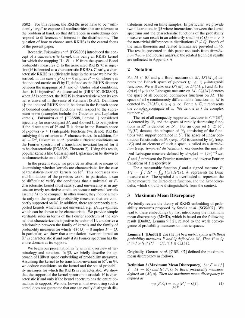
Figure 1: Behavior of the empirical estimate of γ2F (P, Q) w.r.t. ν for the (a) B1-spline kernel and (b) Gaussian kernel. P is

constructed from Q as defined in Eq. (4). “Uniform” corresponds to Q = U [−1, 1] and “Gaussian” corresponds to Q = N (0, 2).m = 1000 samples are generated from P and Q to estimate γ2

F (P, Q) through γ2F,u(m,m). See Example 2 for details.

5 Dissimilar Distributions with Small MeanDiscrepancy

So far, we have studied the behavior of γF and have shownthat it depends on the support of the spectrum of the ker-nel. As mentioned in §1, applications like homogeneity test-ing exploit the metric property of γF to distinguish betweenprobability distributions. Since the metric nature of γF isguaranteed only for kernels with supp(Λ) = Rd, tests basedon other kernels can fail to distinguish between different prob-ability distributions. However, in the following, we showthat the characteristic kernels, while guaranteeing γF to be ametric on S, may nonetheless have difficulty in distinguish-ing certain distributions on the basis of finite samples. Be-fore proving the result, we motivate it through the followingexample.

Example 2 Let P be defined as

p(x) = q(x) + αq(x) sin(νπx), (4)

where q is a symmetric probability density function with α ∈R, ν ∈ R\0. Consider a B1-spline kernel on R given byk(x, y) = ψ(x− y) where

ψ(x) =

1− |x|, |x| ≤ 10, otherwise , (5)

with its Fourier transform given by Ψ(ω) = 2√

2√π

sin2 ω2

ω2 (seefootnote 10 for the definition of Ψ). Since ψ is characteristicto S, γF (P, Q) > 0 (see Theorem 7). However, it would beof interest to study the behavior of γF (P,Q) as a function ofν. We do this through an unbiased, consistent estimator6 ofγ2F (P, Q) as proposed by Gretton et al. [GBR+07, Lemma

7].6Starting from the expression for γF in Eq. (2), we get

γ2F (P, Q) = EX,X′∼P k(X, X ′) − 2EX∼P,Y∼Qk(X, Y ) +EY,Y ′∼Qk(Y, Y ′), where X, X ′ are independent random vari-ables with distribution P and Y, Y ′ are independent randomvariables with distribution Q. An unbiased empirical estimateof γ2

F , denoted as γ2F,u(m, m) is given by γ2

F,u(m, m) =1

m(m−1)

∑ml6=j h(Zl, Zj), which is a one-sample U -statistic with

h(Zl, Zj) := k(Xl, Xj) + k(Yl, Yj) − k(Xl, Yj) − k(Xj , Yl),where Z1, . . . , Zm are m i.i.d. random variables with Zj :=(Xj , Yj) (see [GBR+07, Lemma 7]).

Figure 1(a) shows the behavior of the empirical estimateof γ2

F (P, Q) as a function of ν for q = U [−1, 1] and q =N (0, 2) using the B1-spline kernel in Eq. (5). Since theGaussian kernel, k(x, y) = e−(x−y)2 is also a characteristickernel, its effect on the behavior of γ2

F,u(m,m) is shown inFigure 1(b) in comparison to that of the B1-spline kernel.

From Figure 1, we observe two circumstances under whi-ch the mean discrepancy may be small. First, γ2

F,u(m,m)decays with increasing |ν|, and can be made as small as de-sired by choosing a sufficiently large |ν|. Second, in Fig-ure 1(a), γ2

F,u(m,m) has troughs at ν = ω0π where ω0 =

ω : Ψ(ω) = 0. Since γ2F,u(m,m) is a consistent esti-

mate of γ2F (P, Q), one would expect similar behavior from

γ2F (P, Q). This means that though the B1-spline kernel is

characteristic to S, in practice, it becomes harder to distin-guish between P and Q with finite samples, when P is con-structed as in Eq. (4) with ν = ω0

π . In fact, one can observefrom a straightforward spectral argument that the troughs inγ2F (P, Q) can be made arbitrarily deep by widening q, when

q is Gaussian.

For characteristic kernels, although γF (P, Q) > 0 whenP 6= Q, Example 2 demonstrates that one can constructdistributions such that γ2

F,u(m,m) is indistinguishable fromzero with high probability, for a given sample size m. Below,in Theorem 12, we investigate the decay mode of MMD forlarge |ν| (see Example 2) by explicitly constructing P 6= Qsuch that |Pϕl−Qϕl| is large for some large l, but γF (P, Q)is arbitrarily small, making it hard to detect a non-zero valueof the population MMD on the basis of a finite sample. Here,ϕl ∈ L2(M) represents the bounded orthonormal eigenfunc-tions of a positive definite integral operator7 associated withk.

Consider the formulation of MMD in Eq. (1). The con-struction of P for a given Q such that γF (P, Q) is small,though not zero, can be intuitively seen by re-writing Eq. (1)as

γF (P, Q) = supf∈H

|Pf −Qf |‖f‖H . (6)

7See [SS02, Theorem 2.10] for definition of positive definiteintegral operator and its corresponding eigenfunctions.

When P 6= Q, |Pf − Qf | can be large for some f ∈ H.However, γF (P, Q) can be made small by selecting P suchthat the maximization of |Pf−Qf |

‖f‖H over H requires an f withlarge ‖f‖H. More specifically, higher order eigenfunctionsof the kernel (ϕl for large l) have large RKHS norms, andso if they are prominent in P, Q (i.e., highly non-smoothdistributions), one can expect γF (P,Q) to be small evenwhen there exists an l for which |Pϕl − Qϕl| is large. Tothis end, we need the following lemma, which we quotefrom [GSB+04, Lemma 6].

Lemma 11 ([GSB+04]) Let F be a unit ball in an RKHS(H, k) defined on compact M . Let ϕl ∈ L2(M) be or-thonormal eigenfunctions (assumed to be absolutely bounded),and λl be the corresponding eigenvalues (arranged in a de-creasing order for increasing l) of a positive definite integraloperator associated with k. Assume λ−1

l increases superlin-early with l. Then for f ∈ F where f(x) :=

∑∞j=1 fjϕj(x),

we have |fj |∞j=1 ∈ `1 and for every ε > 0, ∃ l0 ∈ N suchthat |fl| < ε if l > l0.

Theorem 12 (P 6= Q can give small MMD) Assume the con-ditions in Lemma 11 hold. Then there exists a probabilitydistribution P 6= Q defined on M for which |Pϕl −Qϕl| >β − ε for some non-trivial β and arbitrarily small ε > 0, yetfor which γF (P, Q) < η for an arbitrarily small η > 0.

Proof: Let us construct p(x) = q(x) + αle(x) + βϕl(x)where e(x) = 1M (x). For P to be a probability distribution,the following conditions need to be satisfied:

∫

M

[αle(x) + βϕl(x)] dx = 0, (7)

minx∈M

[q(x) + αle(x) + βϕl(x)] ≥ 0. (8)

Expanding e(x) and f(x) in the orthonormal basis ϕl∞l=1,we get e(x) =

∑∞l=1 elϕl(x) and f(x) =

∑∞l=1 flϕl(x),

where el := 〈e, ϕl〉L2(M) and fl := 〈f, ϕl〉L2(M). There-fore, Pf −Qf =

∫M

f(x)[αle(x) + βϕl(x)] dx reduces to

Pf −Qf = αl

∞∑

j=1

ej fj + βfl, (9)

where we used the fact that8 〈ϕj , ϕt〉L2(M) = δjt. RewritingEq. (7) and substituting for e(x) gives

∫M

[αle(x)+βϕl(x)] dx

=∫

Me(x)[αle(x) + βϕl(x)] dx = αl

∑∞j=1 e2

j + βel = 0,which implies

αl = − βel∑∞j=1 e2

j

. (10)

Now, let us consider Pϕt−Qϕt = αlet +βδtl. Substitutingfor αl gives

Pϕt −Qϕt = βδtl − βetel∑∞j=1 e2

j

= βδtl − βτtl, (11)

where τtl := etel∑∞j=1 e2

j. By Lemma 11, |el|∞l=1 ∈ `1 ⇒∑∞

j=1 e2j < ∞, and choosing large enough l gives |τtl| <

8Here δ is used in the Kronecker sense.

ε, ∀ t, for any arbitrary ε > 0. Therefore, |Pϕt − Qϕt| >β− ε for t = l and |Pϕt−Qϕt| < ε for t 6= l. By appealingto Lemma 1, we therefore establish that P 6= Q. In thefollowing we prove that γF (P, Q) can be arbitrarily small,though non-zero.

Recall that γF (P, Q) = sup‖f‖H≤1 |Pf −Qf |. Substi-tuting for αl in Eq. (9), we have

γF (P, Q) = sup

β

∞∑

j=1

νjlfj :∞∑

j=1

f2j

λj≤ 1

, (12)

where we used the definition of RKHS norm as ‖f‖H :=∑∞

j=1

f2j

λjand νjl := δjl− τjl. Eq. (12) is a convex quadratic

program in fj∞j=1. Solving the Lagrangian yields fj =νjlλj√∑∞j=1 ν2

jlλj. Therefore, γF (P, Q) = β

√∑∞j=1 ν2

jlλj =

β√

λl − 2τllλl +∑∞

j=1 τ2jlλj → 0 as l →∞ because

(i) by choosing sufficiently large l, |τjl| < ε, ∀ j, for anyarbitrary ε > 0,(ii) λl → 0 as l →∞ [SS02, Theorem 2.10].

6 Proofs of the Main TheoremsIn this section, we prove the main theorems in Section 4.

6.1 Preliminary lemmasUsing the Fourier characterization of ψ given by Eq. (3), un-der Assumption 1, we derive the following result that pro-vides the Fourier representation of MMD. This result re-quires tools from distribution theory related to the Fouriertransforms of distributions.9 We refer the reader to [Rud91,Chapters 6,7] for the detailed treatment of distribution the-ory. Another good and basic reference on distribution theoryis [Str03].

Lemma 13 (Fourier representation of MMD) Let F be aunit ball in an RKHS (H, k) defined on Rd with k satisfyingAssumption 1. Let φP and φQ be the characteristic functionsof probability measures P and Q defined on Rd. Then

γF (P,Q) = ‖[(φP − φQ)Λ]∨‖H, (13)

where − represents complex conjugation, ∨ represents theinverse Fourier transform and Λ represents the finite non-negative Borel measure on Rd as defined in Eq. (3). (φP −φQ)Λ represents a finite Borel measure defined by Eq. (26).

Proof: From Theorem 3, we have γF (P, Q) = ‖Pk−Qk‖H.Consider Pk =

∫Rd k(·, x) dP (x) =

∫Rd ψ(·−x) dP (x). By

Eq. (23),∫Rd ψ(·−x) dP (x) represents the convolution of ψ

and P , denoted as ψ∗P . By appealing to the convolution the-orem (Theorem 22), we have (ψ∗P )∧ = PΛ, where P (ω) =

9Here, the term distribution should not be confused with proba-bility distributions. In short, distributions refer to generalized func-tions which cannot be treated as functions in the Lebesgue sense.Classical examples of distributions are the Dirac-delta function andHeaviside’s function, for which derivatives and Fourier transformsdo not exist in the usual sense.

∫Rd e−iωT x dP (x), ∀ω ∈ Rd (by Lemma 20). Note that

P = φP . Therefore, γF (P, Q) = ‖ψ ∗ P − ψ ∗Q‖H =∥∥(φP Λ)∨ − (φQΛ)∨∥∥H. Using the linearity of the Fourier

inverse, we get the desired result.

Remark 14 (a) If Ψ is the distributional derivative10 of Λ,then Eq. (13) can also be written as

γF (P, Q) = ‖[(φP − φQ)Ψ]∨‖H, (14)

where the term inside the RKHS norm is the Fourier inverseof a tempered distribution.

(b) By Assumption 1, ψ is real-valued and symmetric in Rd.Therefore, by (ii) in Lemma 20, Λ and Ψ are real-valued,symmetric tempered distributions.

The representation of MMD in terms of the kernel spectrumas in Eq. (13) will be central to deriving our main theorems.It is easy to see that characteristic kernels can be describedindirectly by deriving conditions for the existence of P 6= Qsuch that γF (P,Q) = 0. Using the Fourier representationof γF , the following result provides necessary and sufficientconditions for the existence of P 6= Q such that γF (P, Q) =0.

Lemma 15 Let F be a unit ball in an RKHS (H, k) definedon Rd, and let P,Q be probability distributions on Rd suchthat P 6= Q. Suppose that k satisfies Assumption 1 andsupp(Λ) ⊂ Rd. Then γF (P, Q) = 0 if and only if thereexists θ ∈ S ′

d that satisfies the following conditions:

(i) p− q = θ,(ii) θΛ = 0,

where p and q represent the distributional derivatives of Pand Q respectively, and θΛ represents a finite Borel measuredefined by Eq. (26).

Proof: The proof follows directly from the formulation ofγF in Eq. (13).

(⇒ ) Let θ ∈ S ′d satisfy (i) and (ii). Since θ ∈ S ′

d, we have

θ = ˆθ = (p − q)∧ = p − q = φP − φQ. Therefore, by (ii),we have γF (P,Q) = ‖[(φP −φQ)Λ]∨‖H = ‖[θΛ]∨‖H = 0.

(⇐ ) Let γF (P, Q) = ‖[(φP − φQ)Λ]∨‖H = 0, which im-plies [(φP−φQ)Λ]∨ = 0. Since (φP−φQ)Λ is a finite Borelmeasure as defined by Eq. (26), it is therefore a tempered dis-tribution and so (φP −φQ)Λ = [[(φP −φQ)Λ]∨]∧ = 0. Letθ := φP − φQ. Clearly θ ∈ S ′

d as by Lemma 20, φP , φQ ∈S ′

d. So, p− q = (φP )∨ − (φQ)∨ = (φP − φQ)∨ = θ.

θ = 0 trivially satisfies (ii) in Lemma 15. However, it vio-lates our assumption of P 6= Q when it is used in condition

10If Λ is absolutely continuous w.r.t. the Lebesgue measure,then Ψ represents the Radon-Nikodym derivative of Λ w.r.t. theLebesgue measure. In such a case, ψ is the Fourier transform ofΨ in the usual sense; i.e., ψ(x) =

∫Rd e−ixT ωΨ(ω) dmd(ω). On

the other hand, if Ψ is the distributional derivative of Λ, then Ψ is asymbolic representation of the derivative of Λ and will make senseonly under the integral sign.

(i). If we relax this assumption, then the result is trivial asP = Q ⇒ γF (P, Q) = 0. For the results we derive later,it is important to understand the properties of θ, which wepresent in the following proposition.

Proposition 16 (Properties of θ) θ in Lemma 15 satisfies thefollowing properties:

(a) θ is a conjugate symmetric, bounded and uniformly con-tinuous function on Rd.

(b) θ(0) = 0.

(c) supp(θ) ⊂ Rd\Ω where Ω := supp(Λ). In addition, ifΩ = a1, a2, . . ., then θ(aj) = 0, ∀ aj ∈ Ω.

Proof: (a) From Lemma 15, we have θ = φP − φQ. There-fore, the result in (a) follows from Lemma 20, which showsthat φP , φQ are conjugate symmetric, bounded, and uni-formly continuous functions on Rd.

(b) By Lemma 20, φP (0) = φQ(0) = 1. Therefore, θ(0) =φP (0)− φQ(0) = 0.

(c) Let W := x ∈ Rd | θ(x) 6= 0. It suffices to showthat W ⊂ Rd\Ω. Suppose W is not contained in Rd\Ω.Then there is a non-empty open subset U such that U ⊂W ∩ (Ω ∪ ∂Ω). Fix further a non-empty open subset Vwith V ⊂ U . Since V ⊂ Ω, there is ϕ ∈ Dd(V ) withΛ(ϕ) 6= 0. Take h ∈ Dd(U) such that h = 1 on V , anddefine a continuous function % = hϕ

θ on Rd, which is well-defined from supp(h) ⊂ U and θ 6= 0 on U . By (ii) ofLemma 15, θΛ = 0, where θΛ is a finite Borel measure onRd as defined by Eq. (26). Therefore,

∫

Rd

%(x)θ(x) dΛ(x) = 0. (15)

The left hand side of Eq. (15) simplifies to∫

Rd

%(x)θ(x) dΛ(x) =∫

U

h(x)ϕ(x)θ(x)

θ(x) dΛ(x)

=∫

U

ϕ(x) dΛ(x) = Λ(ϕ) 6= 0,

resulting in a contradiction. So, supp(θ) ⊂ Rd\Ω.If Ω = a1, a2, . . ., then Λ =

∑aj∈Ω βjδaj , βj > 0

and∑

j βj < ∞. θΛ = 0 implies∫Rd χ(x)θ(x) dΛ(x) =∑

j βjχ(aj)θ(aj) = 0 for any continuous function χ in Rd.This implies θ(aj) = 0, ∀ aj ∈ Ω.

Lemma 15 provides conditions under which γF (P, Q) = 0when P 6= Q. It shows that the kernel k cannot distinguishbetween P and Q if P is related to Q by condition (i). Con-dition (ii) in Lemma 15 says that θ has to be chosen suchthat its support is disjoint with that of the kernel spectrum.This is what is precisely captured by (c) in Proposition 16.So, for a given Q, one can construct P such that P 6= Q andγF (P, Q) = 0 by choosing θ that satisfies the properties inProposition 16. However, P should be a positive distributionso that it corresponds to a positive measure.11 Therefore,

11A positive distribution is defined to be as the one that takesnonnegative values on nonnegative test functions. So, D ∈ D ′

d(M)

θ should also be such that q + θ is a positive distribution.Imposing such a constraint on θ is not straightforward, andtherefore Lemma 15 does not provide a procedure to con-struct P 6= Q given Q. However, by imposing some condi-tions on P and Q, we obtain the following result wherein theconditions on θ can be explicitly specified, yielding a proce-dure to construct P 6= Q such that γF (P, Q) = 0.

Lemma 17 Let F be a unit ball in an RKHS (H, k) de-fined on Rd. Let D be the set of probability measures onRd with characteristic functions either absolutely integrableor square integrable, i.e., for any P ∈ D, φP ∈ L1(Rd) ∪L2(Rd). Suppose that k satisfies Assumption 1 and supp(Λ) (Rd. Then for any Q ∈ D, ∃P 6= Q, P ∈ D given by

p = q + θ (16)

such that γF (P, Q) = 0 if and only if there exists a non-zerofunction θ : Rd → C that satisfies the following conditions:

(i) θ ∈ (L1(Rd)∪L2(Rd))∩Cb(Rd) is conjugate symmet-ric,

(ii) θ ∈ L1(Rd) ∩ (L2(Rd) ∪ Cb(Rd)),

(iii) θΛ = 0,

(iv) θ(0) = 0,

(v) infx∈Rdθ(x) + q(x) ≥ 0.

Proof: (⇒ ) Suppose there exists a non-zero function θ sat-isfying (i) – (v). We need to show that p = q + θ is in D forq ∈ D and γF (P, Q) = 0.

For any Q ∈ D, φQ ∈ (L1(Rd) ∪ L2(Rd)) ∩ Cb(Rd).When φQ ∈ L1(Rd)∩Cb(Rd), the Riemann-Lebesgue lemma(Lemma 23) implies that q = [φQ]∨ ∈ L1(Rd) ∩ Cb(Rd).When φQ ∈ L2(Rd) ∩ Cb(Rd), the Fourier transform in theL2 sense12 implies that q = [φQ]∨ ∈ L1(Rd) ∩ L2(Rd).Therefore, q ∈ L1(Rd) ∩ (L2(Rd) ∪ Cb(Rd)). Define p :=q+ θ. Clearly p ∈ L1(Rd)∩(L2(Rd)∪Cb(Rd)). In addition,φP = p = q + ˆθ = φQ + θ ∈ (L1(Rd)∪L2(Rd))∩Cb(Rd).Since θ is conjugate symmetric, θ is real valued and so isp. Consider

∫Rd p(x) dx =

∫Rd q(x) dx +

∫Rd θ(x) dx =

1+θ(0) = 1. (v) implies that p is non-negative. Therefore, Prepresents a probability measure such that P 6= Q and P ∈D. Since P, Q are probability measures, γF (P,Q) is com-puted as γF (P,Q) = ‖[(φP −φQ)Λ]∨‖H = ‖[θΛ]∨‖H = 0.

(⇐ ) Suppose that P, Q ∈ D and p = q+θ gives γF (P,Q) =0. We need to show that θ satisfies (i) – (v).

is a positive distribution if D(ϕ) ≥ 0 for 0 ≤ ϕ ∈ Dd(M). If µ isa positive measure that is locally finite, then Dµ(ϕ) =

∫M

ϕ dµ de-fines a positive distribution. Conversely, every positive distributioncomes from a locally finite positive measure [Str03, §6.4].

12If f ∈ L2(Rd), the Fourier transform z[f ] := f of f isdefined to be the limit, in the L2-norm, of the sequence fn ofFourier transforms of any sequence fn of functions belonging toSd, such that fn converges in the L2-norm to the given functionf ∈ L2(Rd), as n → ∞. The function f is defined almost every-where on Rd and belongs to L2(Rd). Thus, z is a linear operator,mapping L2(Rd) into L2(Rd).

P, Q ∈ D implies φP , φQ ∈ (L1(Rd) ∪ L2(Rd)) ∩Cb(Rd) and p, q ∈ L1(Rd) ∩ (L2(Rd) ∪ Cb(Rd)). There-fore, θ = φP − φQ ∈ (L1(Rd) ∪ L2(Rd)) ∩ Cb(Rd) andθ = p− q ∈ L1(Rd) ∩ (L2(Rd) ∪ Cb(Rd)). By Lemma 20,φP and φQ are conjugate symmetric and so is θ. Thereforeθ satisfies (i) and θ satisfies (ii). θ satisfies (iv) as θ(0) =∫Rd θ(x) dx =

∫Rd(p(x)− q(x)) dx = 0. Non-negativity of

p yields (v). γF (P, Q) = 0 implies (iii), with a proof similarto that of Lemma 15.

Remark 18 Conditions (iii) and (iv) in Lemma 17 are thesame as those of Proposition 16. Conditions (i) and (ii) arerequired to satisfy our assumption P, Q ∈ D and Eq. (16).Condition (v) ensures that P is a positive measure, whichwas the condition difficult to impose in Lemma 15.

In the above result, we restricted ourselves to probabilitymeasures P with characteristic functions φP in L1(Rd) ∪L2(Rd). This ensures that the inverse Fourier transform ofφP exists in the L1 or L2 sense. Without this assumption, φP

is not guaranteed to have a Fourier transform in the L1 or L2

sense, and therefore has to be treated as a tempered distribu-tion for the purpose of computing its Fourier transform. Thisimplies θ = φP−φQ has to be treated as a tempered distribu-tion, which is the setting in Lemma 15. Since we wanted toavoid dealing with distributions where the required positiv-ity constraint is difficult to impose, we restricted ourselves toD.13 Though this result explicitly captures the conditions onθ, it is a very restricted result as it only deals with continuous(a.e.) probability measures. However, we use this result inLemma 19 to construct P 6= Q such that γF (P,Q) = 0.

Lemmas 15 and 17 are the main results that provide con-ditions for the existence of P 6= Q such that γF (P,Q) = 0.This means that if there exists a θ satisfying these condi-tions, then k cannot distinguish between P and Q where Pis defined as in Eq. (16). Thus, the existence (resp. non-existence) of θ results in a non-injective (resp. injective)map Π. It is clear from Lemmas 15 and 17 that the de-pendence of γF on the kernel appears in the form of thesupport of the kernel spectrum. Therefore, two scenariosexist: (a) supp(Λ) = Rd and (b) supp(Λ) ( Rd. Thecase of supp(Λ) = Rd is addressed by Theorem 7 whilethat of supp(Λ) ( Rd is addressed by Theorem 9. Us-ing Lemma 17, the following result proves the existence ofP 6= Q such that γF (P, Q) = 0 while using a kernel withsupp(Λ) ( Rd.

Lemma 19 Let F be a unit ball in an RKHS (H, k) de-fined on Rd. Let D be the set of all non-compactly sup-ported probability measures on Rd with characteristic func-tions in L1(Rd)∪L2(Rd). Suppose k satisfies Assumption 1and supp(Λ) ( Rd. Then ∃P 6= Q, P, Q ∈ D such thatγF (P, Q) = 0.

13Choosing D to be the set of all probability measures with char-acteristic functions in L1(Rd)∪L2(Rd) is the best possible restric-tion that avoids treating θ as a tempered distribution. The classi-cal Fourier transforms on Rd are defined for functions in Lp(Rd),1 < p ≤ 2. For p > 2, the only reasonable way to define Fouriertransforms on Lp(Rd) is through distribution theory.

Proof: We claim that there exists a non-zero function, θ sat-isfying (i) – (v) in Lemma 17 which therefore proves theresult. Consider the following function, gβ,ω0 ∈ C∞(Rd)supported in [ω0 − β, ω0 + β],

gβ,ω0(ω) =d∏

j=1

1[−βj ,βj ](ωj −ω0,j) e− β2

j

β2j−(ωj−ω0,j)2 , (17)

where ω = (ω1, . . . , ωd), ω0 = (ω0,1, . . . , ω0,d) and β =(β1, . . . , βd). Since supp(Λ) ( Rd, there exists an openset U ⊂ Rd on which Λ is null. So, there exists β andω0 6= 0 with ω0 > β such that [ω0 − β, ω0 + β] ⊂ U .Choose θ = α(gβ,ω0 + gβ,−ω0), α ∈ R\0, which im-plies supp(θ) = [−ω0 − β,−ω0 + β] ∪ [ω0 − β, ω0 + β]is compact. Therefore, by the Paley-Wiener theorem (The-orem 24), θ is a rapidly decaying function, i.e., θ ∈ Sd.Since θ(0) = 0 (by construction), θ will take negative val-ues. However, θ decays faster than some Q ∈ D of theform q(x) ∝ ∏d

j=11

1+|xj |l+ε , ∀ l ∈ N, ε > 0 where x =(x1, . . . , xd). It can be verified that θ satisfies conditions (i)– (v) in Lemma 17. We conclude, there exists a non-zero θas claimed earlier, which completes the proof.

The above result shows that k with supp(Λ) ( Rd is notcharacteristic to the class of non-compactly supported prob-ability measures on Rd with characteristic functions in eitherL1(Rd) or L2(Rd).

6.2 Main theorems: ProofsWe are now in a position to prove Theorems 7 and 9.

6.2.1 Proof of Theorem 7(⇒ ) Let supp(Λ) = Rd. k is a characteristic kernel to S ifγF (P, Q) = 0 ⇔ P = Q for P, Q ∈ S. We only need toshow the implication γF (P, Q) = 0 ⇒ P = Q as the otherdirection is trivial.

Assume that ∃P 6= Q such that γF (P,Q) = 0. Thenby Lemma 15, ∃ θ satisfying (i) and (ii) given in Lemma 15.By Proposition 16, θΛ = 0 implies supp(θ) ⊂ Rd\supp(Λ).Since supp(Λ) = Rd and θ is a uniformly continuous func-tion in Rd, we have supp(θ) = ∅ which means θ = 0 a.e.Therefore, by (i) of Theorem 15, we have P = Q, leading toa contradiction. Thus, @P 6= Q such that γF (P, Q) = 0.

(⇐ ) Suppose k is characteristic to S. We then need to showthat supp(Λ) = Rd. This is equivalent to proving that k is notcharacteristic to S when supp(Λ) ( Rd. Let supp(Λ) ( Rd.Choose D ( S as the set of all non-compactly supportedprobability measures on Rd with characteristic functions inL1(Rd)∪L2(Rd). By Lemma 19, ∃P 6= Q, P, Q ∈ D ( Ssuch that γF (P,Q) = 0. Therefore, k is not characteristic toS.

6.2.2 Proof of Theorem 9Suppose ∃P 6= Q, P, Q ∈ D ( S such that γF (P, Q) = 0.Then by Lemma 15, there exists a θ ∈ S ′

d such that θ = p−qwhere p and q are the distributional derivatives of P and Q,respectively. Since P, Q ∈ D, we can apply Lemma 17 andso θ is a non-zero function that satisfies conditions (i) – (v)in Lemma 17. The condition θΛ = 0 implies supp(θ) ⊂

Rd\supp(Λ). Since supp(Λ) has a non-empty interior, wehave supp(θ) ( Rd. Thus, there exists an open set, U ⊂ Rd

such that θ(x) = 0, ∀x ∈ U . By Lemma 25, this means thatθ is not compactly supported in Rd. Condition (iv) implies∫Rd θ(x) dx = 0, which means that θ takes negative values.

Since q is compactly supported in Rd, q(x) + θ(x) < 0for some x ∈ Rd\supp(Q), which violates condition (v) inLemma 17. In other words, there does not exist a non-zero θthat satisfies conditions (i) – (v) in Lemma 17, thereby lead-ing to a contradiction.

As discussed in §4.1, the condition that supp(Λ) has a non-empty interior is important for Theorem 9 to hold. This is be-cause if supp(Λ) has an empty interior, then supp(θ) = Rd.In principle, one can construct such a θ by selecting θ ∈ Sd

so that it satisfies conditions (i) – (iv) of Lemma 17 while sat-isfying the decay conditions (Eq. (29) and Eq. (30)) given inthe Paley-Wiener theorem (see Theorem 24). Therefore, bythe Paley-Wiener theorem, θ is a C∞ function with compactsupport. If θ is chosen such that supp(θ) ⊂ supp(Q), thencondition (v) of Theorem 17 will be satisfied. Thus, one canconstruct P 6= Q, P, Q ∈ D (D being defined in Theorem 9)such that γF (P,Q) = 0. Note that conditions (i) and (ii) ofLemma 17 are automatically satisfied (except for conjugatesymmetry) by choosing θ ∈ Sd. However, choosing θ suchthat it is also an entire function (so that the Paley-Wiener the-orem can be applied) is not straightforward. In the following,we provide a simple example to show that P 6= Q, P, Q ∈ Dcan be constructed such that γF (P, Q) = 0, where F corre-sponds to a unit ball in an RKHS (H, k) induced by a pe-riodic translation-invariant kernel for which supp(Λ) ( Rd

has an empty interior.

Example 3 Let Q be a uniform distribution on [−β, β] ⊂ R,i.e., q(x) = 1

2β1[−β,β](x) with its characteristic function,

φQ(ω) = 1β√

2π

sin(βω)ω in L2(R). Let ψ be the Dirichlet ker-

nel with period τ , where τ ≤ β, i.e., ψ(x) = sin(2l+1)πx

τ

sin πxτ

and

Ψ(ω) =∑l

j=−l δ(ω − 2πj

τ

)with supp(Ψ) = 2πj

τ , j ∈0,±1, . . . ,±l. Clearly, supp(Ψ) has an empty interior.Let θ be

θ(ω) =8√

2α

i√

πsin

(ωτ

2

) sin2(

ωτ4

)

τω2, (18)

with α ≤ 12β . It is easy to verify that θ ∈ L1(R) ∩ L2(R) ∩

Cb(R) and so θ satisfies (i) in Lemma 17. Since θ(ω) = 0 atω = 2πl

τ , l ∈ Z, θ also satisfies (iii) and (iv) in Lemma 17.θ is given by

θ(x) =

2α|x+ τ2 |

τ − α, −τ ≤ x ≤ 0

α− 2α|x− τ2 |

τ , 0 ≤ x ≤ τ0, otherwise,

(19)

where θ ∈ L1(R)∩L2(R)∩Cb(R) satisfies (ii) in Lemma 17.Now, consider p = q + θ which is given as

p(x) =

12β , x ∈ [−β,−τ ] ∪ [τ, β]

2α|x+ τ2 |

τ + 12β − α, x ∈ [−τ, 0]

α + 12β −

2α|x− τ2 |

τ , x ∈ [0, τ ]0, otherwise.

Clearly, p(x) ≥ 0, ∀x and∫R p(x) dx = 1. φP = φQ +θ =

φQ + iθI where θI = Im[θ] and φP ∈ L2(R). We havetherefore constructed P 6= Q such that γF (P, Q) = 0, whereP and Q are compactly supported in R with characteristicfunctions in L2(R).

The condition of the compact support for probability mea-sures mentioned in Theorem 9 is also critical for the result tohold. If this condition is relaxed, then k with supp(Λ) ( Rd

is no longer characteristic to D, as shown in Lemma 19.

7 Concluding RemarksPrevious works have studied the Hilbert space embedding forprobability measures using universal kernels, which form arestricted family of positive definite kernels. These worksshowed that if the kernel is universal, then the embeddingfunction from the space of probability measures to a repro-ducing kernel Hilbert space is injective. In this paper, weextended this approach to a larger family of kernels whichare translation-invariant on Rd. We showed that the supportof the Fourier spectrum of the kernel determines whether theembedding is injective. In particular, the necessary and suf-ficient condition for the embedding to be injective is that theFourier spectrum of the kernel should have the entire domainas its support. Our study in this paper was limited to ker-nels and probability measures that are defined on Rd, andthe results have been derived using Fourier analysis in Rd.Since Fourier theory is available for more general groupsapart from Rd, one direction for future work is to extend theanalysis to positive definite kernels defined on other groups.

Appendix A Supplementary ResultsWe show five supplementary results used to prove the re-sults in §4 and §6. The first two are basic, and deal withthe Fourier transform of a measure and the convolution the-orem. The remaining three (the Riemann-Lebesgue lemma,the Paley-Wiener theorem, and its corollary) are stated with-out proof.

Lemma 20 (Fourier transform of a measure) Let µ be a fi-nite Borel measure on Rd. The Fourier transform of µ is atempered distribution given by

µ(ω) =∫

Rd

e−iωT x dµ(x), ∀ω ∈ Rd (20)

which is a bounded, uniformly continuous function on Rd. Inaddition, µ satisfies the following properties:

(i) µ(ω) = µ(−ω), ∀ω ∈ Rd,

(ii) µ(ω) = µ(−ω), ∀ω ∈ Rd if and only if Dµ(ϕ) =Dµ(ϕ), ∀ϕ ∈ Sd where Dµ is the tempered distribu-tion defined by µ and ϕ(x) := ϕ(−x), ∀x ∈ Rd.

Proof: Let Dµ denote a tempered distribution defined by µ.For ϕ ∈ Sd, we have Dµ(ϕ) = Dµ(ϕ) =

∫Rd ϕ(ω) dµ(ω) =∫

Rd

∫Rd e−iωT xϕ(x) dmd(x) dµ(ω). From Fubini’s theorem,

Dµ(ϕ) =∫

Rd

[∫

Rd

e−ixT ω dµ(ω)]

ϕ(x) dmd(x), (21)

which proves Eq. (20). Clearly µ is bounded as |µ(ω)| ≤ 1.By Lebesgue’s dominated convergence theorem, µ is uni-formly continuous on Rd as limh→0 |µ(ω + h) − µ(ω)| ≤limh→0

∫Rd |e−jhT x − 1| dµ(x) = 0, for any ω ∈ Rd.

(i) µ(ω) =∫Rd eiωT x dµ(x) = µ(−ω).

(ii) (⇒ ) For ϕ ∈ Sd, Dµ(ϕ) = Dµ(ϕ) =∫Rd ϕ(x) dµ(x) =∫

Rd µ(x)ϕ(x) dmd(x). Since ϕ ∈ Sd and Dµ(ϕ) = Dµ(ϕ),∀ϕ ∈ Sd, we have Dµ(ϕ) = Dµ( ˜ϕ) =

∫Rd ϕ(−x) dµ(x).

Substituting for ϕ(−x), we get

Dµ(ϕ) =∫

Rd

µ(−x)ϕ(x) dmd(x) =∫

Rd

µ(x)ϕ(x) dmd(x),

for every ϕ ∈ Sd, which implies µ(x) = µ(−x), ∀x ∈ Rd.

(⇐ ) For ϕ ∈ Sd, we have Dµ(ϕ) = (Dµ)∨(ϕ) = Dµ(ϕ) =∫Rd µ(x)ϕ(x) dmd(x) =

∫Rd µ(−x)ϕ(x) dmd(x). Apply-

ing Fubini’s theorem after substituting for µ(−x) and ϕ(x)gives

Dµ(ϕ) =∫

Rd

∫

Rd

δ(y + ω)ϕ(y) dmd(y) dµ(ω)

=∫

Rd

ϕ(−ω) dµ(ω) = Dµ(ϕ),

for every ϕ ∈ Sd.

Remark 21 (a) Property (i) in Lemma 20 shows that theFourier transform of a finite Borel measure on Rd is “conju-gate symmetric”, which means that Re[µ] is an even functionand Im[µ] is an odd function.

(b) Property (ii) shows that real symmetric tempered distri-butions have real symmetric Fourier transforms. This can beeasily understood when µ is absolutely continuous w.r.t. theLebesgue measure. Suppose dµ = Ψ dmd. Then property(ii) implies that µ is real and symmetric if and only if Ψ isreal and symmetric.

The following result is popularly known as the convolutiontheorem. Before providing the result, we first define convo-lution: if f and g are complex functions in Rd, their convo-lution f ∗ g is

(f ∗ g)(x) =∫

Rd

f(y)g(x− y) dy, (22)

provided that the integral exists for almost all x ∈ Rd, in theLebesgue sense. Let µ be a finite Borel measure on Rd andf be a bounded measurable function on Rd. The convolutionof f and µ, f ∗ µ, which is a bounded measurable function,is defined by

(f ∗ µ)(x) =∫

Rd

f(x− y) dµ(y). (23)

Theorem 22 (Convolution Theorem) Let µ be a finite Borelmeasure and f be a bounded function on Rd. Suppose f iswritten as

f(x) =∫

Rd

eixT ω dΛ(ω), (24)

with a finite Borel measure Λ on Rd. Then

(f ∗ µ)∧ = µΛ, (25)

where the right hand side is a finite Borel measure14 and theequality holds as a tempered distribution.

Proof: Since the Fourier and inverse Fourier transform giveone-to-one correspondence of S ′

d, it suffices to show

f ∗ µ = (µΛ)∨. (27)

For an arbitrary ϕ ∈ Sd,

(µΛ)∨(ϕ) = (µΛ)(ϕ) =∫

Rd

ϕ(x)µ(x) dΛ(x). (28)

Substituting for µ in Eq. (28) and applying Fubini’s theorem,we have (µΛ)∨(ϕ) =

∫

Rd

∫

Rd

[∫

Rd

ei(ω−y)T x dΛ(x)]

ϕ(ω) dmd(ω) dµ(y),

which reduces to∫Rd [

∫Rd f(ω − y) dµ(y)]ϕ(ω) dmd(ω) =

(f ∗ µ)(ϕ) and therefore proves Eq. (27).

The following result, called the Riemann-Lebesgue lemma,is quoted from [Rud91, Theorem 7.5].

Lemma 23 (Riemann-Lebesgue) If f ∈ L1(Rd), then f ∈Cb(Rd), and ‖f‖∞ ≤ ‖f‖1.

The following theorem is a version of the Paley-Wiener the-orem for C∞ functions, and is proved in [Str03, Theorem7.2.2].

Theorem 24 (Paley-Wiener) Let f be a C∞ function sup-ported in [−β, β]. Then f(ω + iσ) is a entire function ofexponential type β, i.e., ∃C such that

∣∣∣f(ω + iσ)∣∣∣ ≤ Ceβ|σ|, (29)

and f(ω) is rapidly decreasing, i.e., ∃ cn such that∣∣∣f(ω)

∣∣∣ ≤ cn

(1 + |ω|)n, ∀n ∈ N. (30)

Conversely, if F (ω + iσ) is an entire function of exponentialtype β, and F (ω) is rapidly decaying, then F = f for somesuch function f .

The following lemma is a corollary of the Paley-Wiener the-orem, and is proved in [Mal98, Theorem 2.6].

Lemma 25 ([Mal98]) If g 6= 0 has compact support, thenits Fourier transform g cannot be zero on a whole interval.Similarly, if g 6= 0 has compact support, then g cannot bezero on a whole interval.

14Let µ be a finite Borel measure and f be a bounded measurablefunction on Rd. We then define a finite Borel measure fµ by

(fµ)(E) =

∫

Rd

IE(x)f(x) dµ(x), (26)

where E is an arbitrary Borel set and IE is its indicator function.

References[Aro50] N. Aronszajn. Theory of reproducing kernels.

Trans. Amer. Math. Soc., 68:337–404, 1950.[BJ02] F. R. Bach and M. I. Jordan. Kernel independent

component analysis. Journal of Machine Learn-ing Research, 3:1–48, 2002.

[Dud02] R. M. Dudley. Real Analysis and Probability.Cambridge University Press, Cambridge, UK,2002.

[FGSS08] K. Fukumizu, A. Gretton, X. Sun, andB. Scholkopf. Kernel measures of conditionaldependence. In J.C. Platt, D. Koller, Y. Singer,and S. Roweis, editors, Advances in Neural In-formation Processing Systems 20, pages 489–496, Cambridge, MA, 2008. MIT Press.

[GBR+07] A. Gretton, K. M. Borgwardt, M. Rasch,B. Scholkopf, and A. Smola. A kernel methodfor the two sample problem. In B. Scholkopf,J. Platt, and T. Hoffman, editors, Advancesin Neural Information Processing Systems 19,pages 513–520. MIT Press, 2007.

[GHS+05] A. Gretton, R. Herbrich, A. Smola, O. Bousquet,and B. Scholkopf. Kernel methods for measur-ing independence. Journal of Machine LearningResearch, 6:2075–2129, December 2005.

[GSB+04] A. Gretton, A. Smola, O. Bousquet, R. Herbrich,B. Scholkopf, and N. Logothetis. Behaviourand convergence of the constrained covariance.Technical Report 130, MPI for Biological Cy-bernetics, 2004.

[GW99] C. Gasquet and P. Witomski. Fourier Analysisand Applications. Springer-Verlag, New York,1999.

[Mal98] S. G. Mallat. A Wavelet Tour of Signal Process-ing. Academic Press, San Diego, 1998.

[RS72] M. Reed and B. Simon. Functional Analysis.Academic Press, New York, 1972.

[Rud91] W. Rudin. Functional Analysis. McGraw-Hill,USA, 1991.

[SGSS07] A. J. Smola, A. Gretton, L. Song, andB. Scholkopf. A Hilbert space embedding fordistributions. In Proc. 18th International Con-ference on Algorithmic Learning Theory, pages13–31. Springer-Verlag, Berlin, Germany, 2007.

[Sho00] G. R. Shorack. Probability for Statisticians.Springer-Verlag, New York, 2000.

[SS02] B. Scholkopf and A. J. Smola. Learning withKernels. MIT Press, Cambridge, MA, 2002.

[Ste02] I. Steinwart. On the influence of the kernelon the consistency of support vector machines.Journal of Machine Learning Research, 2:67–93, 2002.

[Str03] R. S. Strichartz. A Guide to Distribution Theoryand Fourier Transforms. World Scientific Pub-lishing, Singapore, 2003.

[Wen05] H. Wendland. Scattered Data Approximation.Cambridge University Press, Cambridge, UK,2005.