Activity and Gait Recognition with Time-Delay Embeddings

Jordan FrankDepartment of Computer Science

McGill University, Montreal, Canadajordan.frank@cs.mcgill.ca

Shie MannorFaculty of Electrical Engineering

The Technion, Haifa, Israelshie@ee.technion.ac.il

Doina PrecupDepartment of Computer Science

McGill University, Montreal, Canadadprecup@cs.mcgill.ca

Abstract

Activity recognition based on data from mobile wearable de-vices is becoming an important application area for machinelearning. We propose a novel approach based on a combina-tion of feature extraction using time-delay embedding and su-pervised learning. The computational requirements are con-siderably lower than existing approaches, so the processingcan be done in real time on a low-powered portable devicesuch as a mobile phone. We evaluate the performance of ouralgorithm on a large, noisy data set comprising over 50 hoursof data from six different subjects, including activities such asrunning and walking up or down stairs. We also demonstratethe ability of the system to accurately classify an individualfrom a set of 25 people, based only on the characteristics oftheir walking gait. The system requires very little parametertuning, and can be trained with small amounts of data.

IntroductionMobile devices are ubiquitous in modern society. Manyof these devices come equipped with sensors such as ac-celerometers and Global Positioning Systems (GPS) that cancollect data about the movements of a user. This creates thepotential of intelligent applications that recognize the user’sactivity and take appropriate action. For example, a devicemight notice that a user is in distress and alert a care giver, orit might make decisions regarding whether incoming phonecalls should be put through or saved in a message box.

Applications for recognizing activities from sensor datahave been developed in a wide range of fields such as healthcare (Kang et al. 2006), fitness (Lester, Choudhury, andBorriello 2006), and security (Kale, Cuntoor, and Chel-lappa 2002). Different types of sensors have been used,e.g., accelerometer data for recognizing physical activities(Lester, Choudhury, and Borriello 2006) and both mobilephone usage data (Farrahi and Gatica-Perez 2008) and GPSdata (Krumm and Horvitz 2006; Liao, Fox, and Kautz 2007)for analyzing human mobility and other higher-level, tem-porally extended activities (Eagle and Pentland 2006).

Our focus is on detecting primitive physical activities(e.g., walking, running, biking, etc.) from data collected us-ing accelerometers built into wearable sensing devices. Pre-vious work on this problem has shown recognition accuracy

Copyright c© 2010, Association for the Advancement of ArtificialIntelligence (www.aaai.org). All rights reserved.

above 85% on large, complex data sets (Subramanya et al.2006; Lester, Choudhury, and Borriello 2006). These exist-ing approaches use standard (mostly linear) signal process-ing methods, through which hundreds of signal statistics arecomputed. Heavy-duty feature extraction tools are then usedto determine which of these features are useful for classifi-cation. While these approaches work well, they require a lotof computing power, so they are not well suited for real-timedetection of activities on low-powered devices.

In this work, we propose an alternative method for rep-resenting time series data that greatly reduces the memoryand computational complexity of performing activity recog-nition. We adopt techniques from nonlinear time series anal-ysis (Kantz and Schreiber 2004) to extract features from thetime series, and use these features as inputs to an off-the-shelf classifier. Additionally, we present a novel approachfor classifying time series data using nonparametric nonlin-ear models that can be built from small data sets. This al-gorithm has been implemented and is able to perform clas-sification of activities in real time on an HTC G1 c© (alsoknown as Dream in some countries) mobile phone.

We will focus in particular on accelerometer data; intu-itively, the acceleration recorded by the device is the resultof a measurement performed on a non-linear dynamical sys-tem, consisting of the hips and legs, with their joints, actu-ations and interaction with the ground. Time-delay embed-ding methods, e.g., (Sauer, Yorke, and Casdagli 1991), pro-vide approaches for reconstructing the essential dynamicsof the underlying system using a short sequence of measure-ments, evenly spaced in time. Assuming that the dynamicsof the underlying system are noticeably different when a per-son is performing different activities, the parameters of thedifferent time-delay embedding models can be used to clas-sify new data. Our approach achieves very good classifica-tion performance, comparable to the state-of-art approaches,but extracts fewer than a dozen features from the time seriesdata, instead of hundreds. The memory and computationalsavings are crucial, given that for many applications, activityrecognition would have to run in real time as a small com-ponent of larger system on a low-powered mobile device.

The main contributions of this paper are twofold. First,we propose the use of the reconstructed coordinates in atime-delay embedding of a time series as input to a super-vised learning algorithm for time series classification. While

time-delay values have been used as input to neural networks(Waibel et al. 1989), the novelty of our approach is in the in-corporation of noise-reduction and the explicit treatment ofthe dynamics. Second, we propose a lightweight classifica-tion algorithm based on time-delay embeddings that is effi-cient enough to run in real time on a low-powered device.Both methods are empirically validated on noisy real-worlddata.

Time-Delay EmbeddingsIn this section we present a brief overview of time-delay em-beddings. We refer the reader to the standard text by Kantzand Schreiber (Kantz and Schreiber 2004) for further de-tails. The purpose of time-delay embeddings is to recon-struct the state and dynamics of an unknown dynamical sys-tem from measurements or observations of that system takenover time. The state of the dynamical system at time t isa point xt ∈ Rk containing all the information necessary tocompute the future of the system at all times following t.The set of all states is called the phase space. Of course, thestate of the system cannot be measured directly, and even thetrue dimension of the phase space k is typically unknown.However, we assume access to a time series 〈ot = ω(xt)〉generated by a measurement function ω : Rk → R, whichis a smooth map from the phase space to a scalar value.Throughout this paper, we use “smooth” to mean contin-uously differentiable. In general, it is hard to reconstructthe state just by looking at the current observation. How-ever, by considering several past observations taken at timest, t − δ1, . . . t − δm−1, the reconstruction should be easier toperform. These m measurements can be considered as pointsin Rm, which is called the reconstruction space. The keyproblem is to determine how many measurements m have tobe considered (i.e., what is the dimension of the reconstruc-tion space), and at what times they should be taken (i.e.,what are the values of δi), in order to capture well the sys-tem dynamics. In particular, if we consider the map from Rk

to Rm (corresponding to taking the measurements and thenprojecting the time series data into the reconstruction space)we would like this map to be one-to-one and to preserve lo-cal structure. If this were the case, by looking at the timeseries in Rm, one would essentially have all the informationfrom the true system state and dynamics.

We consider the time-delay reconstruction in m dimen-sions with time delay τ, which is formed by the vectorsot ∈ Rm, defined as: ot = (ot ,ot+τ,ot+2τ, . . . ,ot+(m−1)τ). Weassume that the true state of the system xt lies on an attrac-tor A ⊂ Rk in an unknown phase space of dimension k. Weuse the term “attractor”, as in dynamical system theory, tomean a closed subset of states towards which the systemwill evolve from many different initial conditions. Once thestate of the system reaches an attractor, it will typically re-main inside it indefinitely (in the absence of external pertur-bations). An embedding is a map from the attractor A intoreconstruction space Rm that is one-to-one and preserves lo-cal differential structure. Takens (1981) showed that if A isa d-dimensional smooth compact manifold, then providedthat m > 2d, τ > 0, and the attractor contains no periodic or-

!"##########!$###########!%###########&############%###########$

& '& ('& %&& %'&)*+,#-./+01,.2

344,1,56+,7,5#8/9:*7;<,#-92

'

&

!'

(&'

&!'

!"!$!%&%$"

!"##########!$###########!%###########&############%###########$

& '& ('& %&& %'&)*+,#-./+01,.2

344,1,56+,7,5#8/9:*7;<,#-92

'

&

!'

(&'

&!'

!"!$!%&%$"

!"##########!$###########!%###########&############%###########$

& '& ('& %&& %'&)*+,#-./+01,.2

344,1,56+,7,5#8/9:*7;<,#-92

'

&

!'

(&'

&!'

!"!$!%&%$"

Figure 1: Example of time-delay embedding for accelerometerdata from biking activity. Left: raw accelerometer data. Right:time-delay embedding with m = 6,τ = 11, p = 3. The colouredpoints in the left diagram are mapped to the same coloured pointsin the embedding.

bits of length τ or 2τ and only finitely many periodic orbitsof length 3τ,4τ, . . . ,mτ, then for almost every smooth func-tion ω, the map from Rk to the time-delay reconstruction isan embedding. In other words, any time-delay reconstruc-tion will accurately preserve the dynamics of the underly-ing dynamical system, provided that m is large enough andτ does not conflict with any periodic orbits in the system.However, from the point of view of activity recognition, wewould like m to be as small as possible, as it determines theminimum time interval after which an activity can be recog-nized. More precisely, if the data is sampled at a rate of rmeasurements per second, then the time window needed forthe time-delay reconstruction is ((m−1)τ+1)/r seconds.

Takens’ theorem only holds when the measurement func-tion ω is deterministic, but in practice all measurements arecorrupted by noise from a variety of sources, ranging fromthe measurement apparatus to rounding errors due to finiteprecision. In the presence of noise, the choice of m and τ

becomes very important. There are a number of techniquesfor choosing good values for m and τ based on geometricaland spectral properties of the data (Buzug and Pfister 1992).However, in our experiments, we found that grid search overa small parameter space, using a small validation data setand optimizing classification accuracy on it, suffices to findgood parameters.

Methods developed for nonlinear time series analysishave not been widely used in the machine learning commu-nity1, but are quite popular in other areas of research. In thefollowing section, we explain how we use time-delay em-beddings for the purpose of classifying time series data.

Proposed ApproachThe main idea of our approach is to extract features usingtime-delay embeddings, followed by a noise-reduction step.Then we use these features as input to a classifier. Definethe time-delay embedding function T (o,m,τ) which takesas parameters a time series o = 〈oi〉Ni=1, and the time-delayembedding parameters m and τ. Let M = N− (m−1)τ. Thefunction T returns an m×M, matrix O whose ith column isthe ith time-delay vector (oi,oi+τ,oi+2τ, . . . ,oi+(m−1)τ).

1The obvious exception is the time-delay neural network re-search. However these methods do not consider noise reduction,or other transformations on these models, they simply use laggedtime sequences as inputs to a network.

For the noise reduction step, principal component analysis(PCA) is performed on the embedding of a short segment ofthe training data (Jolliffe 2002). PCA computes a projectionmatrix P from the time-delay embedding space to a space oflower dimension p, which we will call model space. Oncethe projection matrix P has been computed, any sequenceof observations can be projected into the model space bycomputing the time delay embedding , centering the data bysubtracting its mean, then multiplying by P.

Figure 1 illustrates the concept of time-delay embeddingusing accelerometer data collected from a subject riding astationary bicycle. On the top is a short segment that wasused to find the projection P. The parameters used, m = 6,τ = 11, and p = 3, were chosen based on previous experi-ments. On the bottom is the result of embedding the entiredata set and then projecting onto the basis specified by P.Observe that the system evolves along a set of tightly clus-tered trajectories, in a periodic fashion. This is quite intu-itive, considering that cycling involves a periodic, roughlytwo-dimensional leg movement. However, it is remarkablethat this structure can be reconstructed automatically fromthe time series on the top, especially since the data is non-stationary (i.e., the peaks do not have the same magnitude,and the period varies over time). Note that the colours areonly used as a visual aid, to show where different regionsfrom the time series get mapped in the final model space.

Given a sequence of observations, the computation de-scribed above will produce a matrix whose columns forma sequence of points in the p-dimensional Euclidean modelspace, representing the states of the dynamical system. Wecall this sequence of points a model. The coordinates ofthese points can be used as input features to a learning al-gorithm. However, we can also treat subsequent pairs ofpoints as Euclidean vectors, and look for richer informationon the dynamics of the system. In the next section, we de-scribe a novel learning algorithm that exploits this aspect toour advantage.

Geometric Template Matching AlgorithmThe geometric template matching (GTM) algorithm is an ef-ficient algorithm for assessing how well a given time seriesmatches a particular model. The time series is projected intomodel space, then short segments of the projected data arecompared geometrically against their nearest neighbours inthe model. We treat subsequent pairs of points in modelspace as vectors. Segments of the projected data set thatare geometrically similar to nearby vectors in the modelare given higher scores, while segments that differ from themodel are given low scores.

The algorithm, presented in Algorithm 1, takes as input atime series and a model, and computes nearest-neighboursfor the time series based on Euclidean distance. A set ofscores for each segment of the time series is returned as aresult. In the algorithm, we denote the Euclidean norm by|u|, and the dot product of two vectors u · v. For notationalconvenience we write the vector going from point a to pointb as [a,b].

For classification purposes, one can simply assign to thesequence the class label associated with the model that ob-

Algorithm 1 Geometric Template Matching

Input: Model u = 〈ui〉Ni=1, parameters (m,τ, p,P), sequencelength s, neighbourhood size n, and the sequence to score,o = 〈oi〉Ti=1.Output: A set of scores, r1, . . . ,rT−(m−1)τ−s ∈ [−s,s].

1. Initialize the score, ri = 0 for i = 1, . . . ,(M− s).2. Compute matrix V that represents the model for sequence o,

whose columns form the sequence 〈vi〉Mi=1, where M = T −(m−1)τ.

3. Repeat for i = 1, . . . ,(M− s):Repeat for j = i, . . . ,(i+ s−1):a. Let w1, . . . ,wn be the indices of the n nearest neighbours

of v j in u.b. Let u be the mean of the vectors

[uw1 ,uw1+1], . . . , [uwn ,uwn+1].c. Let v be the vector [v j,v j+1].d. Update the score, ri = ri +(u ·v)/max(|u|, |v|).

4. Return the scores, r1, . . . ,rT−(m−1)τ−s.

tains the highest average score. In order to perform classifi-cation in real-time, as opposed to using batch input, a bufferof the most recent (m− 1)τ+ s samples is maintained, andthe GTM algorithm is run on the buffered data (which willresult in one iteration of the outer loop, and thus one score)as new data become available. In our experiments, we areable to compute a score for 8 models twice per second usingthe embedding parameters m = 12,τ = 2, p = 6, s = 32, andn = 4, with no noticeable impact on the performance of thephone.

ExperimentsWe demonstrate our approach in two experiments focusingon identifying activities and users, respectively.

Activity RecognitionThe data set used for the activity recognition experiment wascollected using the Intel Mobile Sensing Platform (MSP)(Choudhury et al. 2008) that contains a number of sensorsincluding a 3-axis accelerometer and a barometric pressuresensor; these are the only sensors we will use. Six partic-ipants were outfitted with the MSP units, which clip ontoa belt at the side of the hip, and data was collected froma series of 36 two-hour excursions (6 per user) which tookplace over a period of three weeks. The participants wereaccompanied by an observer who recorded the labels as theactivities were being performed. The labels were: walking,lingering, running, up stairs, downstairs, and riding in a ve-hicle. We omitted the vehicle activity for now (because weare not processing GPS signal). Taking into account equip-ment failures and data with obvious errors in the labelling,the working data set consists of 50 hours of labeled data,roughly equally distributed among the six participants.

The accelerometer data is sampled at 512Hz, which wedecimate to 32Hz. The accelerometer data consists of threemeasurements at each time step, corresponding to the accel-eration along each of the three axes, x, y, and z. We combinethese three measurements to form a single measure of the

!"#$%&'())%*(+$'

&'())%*(+$'%,))-./$0%+1%234 5%'-/.$"5%6('75%"#/

8 9888 :8888 :9888 ;8888 ;9888 <8888!-=$%>)(=?'$)@

A%%(BB$'A%%+("C=$D$"

5%#?)D(-")5%0C6/)D(-")

Figure 2: Classification results on a segment of the data from user6 using a classifier trained on user 4. The top coloured bar abovethe data shows the labels assigned by a human labeller and the bot-tom coloured bar shows labels assigned by the classifier. The blackline shows the magnitude of the accelerometer data and the red lineis the gradient of the barometric pressure.

magnitude of the acceleration vector a =√

x2 + y2 + z2−g,where g = 9.8m/s2 is the Earth’s gravity. Subtracting gcauses the acceleration when the device is at rest or mov-ing at a constant velocity to be 0. The barometric pressure issampled at 7.1Hz, smoothed, and then upsampled to 32Hz.The gradient of the signal is used as an additional feature.

For the experiment, we split the data set up into six parts,each containing the data from a specific participant. Webegan by projecting all of the accelerometer data into atime-delay reconstruction space with parameters τ = 3 andm = 16. For each user, we constructed a training set by se-lecting randomly 25% of these embedded data points. Thiscorresponds to approximately 2 hours of data, or 230,000samples for each participant. Next, we performed PCA onthe data points in the training set. We then projected all thereconstructed accelerometer data onto the principal compo-nents corresponding to the 9 largest eigenvalues from thetraining data. This produces 9 features for each data pointin the original time series, and we combined these featureswith the barometric pressure to form the input features fora Support Vector Machine (SVM) classifier (Cristianini andShawe-Taylor 2000). As a basis for comparison, we alsotrained an SVM just using the raw accelerometer value andgradient of the barometric pressure as inputs at each timestep.

We tested each classifier on the entire data set for eachuser. The results are shown in Table 1. The first row con-tains the results when training using only the single raw ac-celerometer value and the gradient of the barometric pres-sure, trained on data from User 1, and testing on all of theusers. It is clear that using features obtained by time-delayembeddings significantly improves classifier performance.Figure 2 shows the result of using the SVM trained on User3 to label a segment of the data for User 6.

The classifier performs well across all users, regardlessof the user on which it was trained. The average accuracyfor the experiments using the time-delay embedding on theentire data set is 85.48±0.30%. This result demonstratesthat these features are useful for activity recognition devices,because the system can be calibrated on one user, then de-

0 50 100 150 200 250 300 350 4004

2

0

2

4

6

Time (samples)Acc

eler

omet

er M

agni

tude

(m/s

2 )

Figure 3: An example segment of the accelerometer data.

ployed to other users, and the performance is very similar(the accuracy loss, as can be seen from the table, is 1-5%).

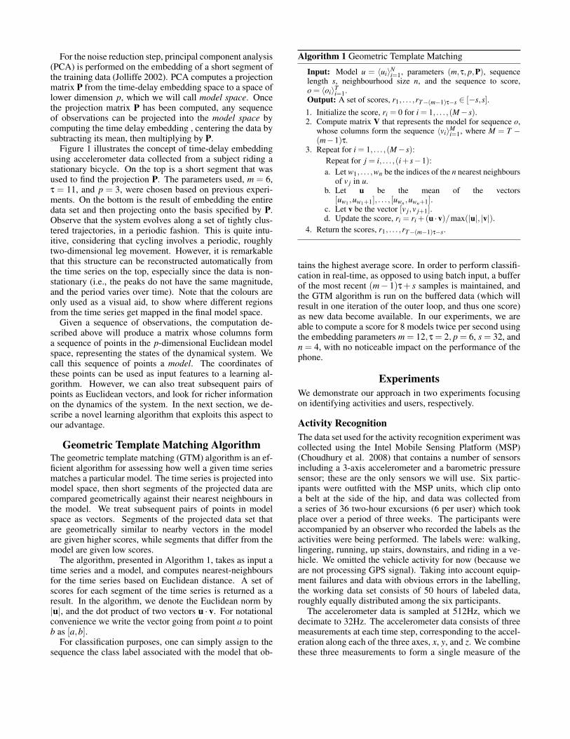
Gait RecognitionGait recognition is the problem of identifying a person bytheir manner of walking, or carriage. The problem of gaitrecognition has been studied in depth in the computer visionand biomechanics communities, where the goal is to identifyan individual based on a sequence of images or silhouettescaptured while the individual is walking (Nixon, Tan, andChellappa 2006). Recent work has considered gait recogni-tion using wearable sensors as a means for biometric iden-tification (Gafurov, Snekkenes, and Bours 2007). For ourexperiment, we implemented a data collection and analysistool for the Google Android operating system, which runs onthe HTC G1 c© mobile phone. In our experiments, the phonewas placed in the front trouser pocket of an individual, andcollected data from the 3-axis accelerometer in the device ata rate of 25Hz2 as the subject walked. We collected a set of25 traces, each containing between 12 and 120 seconds ofcontinuous walking data from one of 25 individuals.

The data was trimmed to remove the time before and af-ter the walk, and the first and last few steps, but no otherpost-processing was performed. Figure 3 contains a shortsequence from one of the data sets. As we can see, the datais noisy, and there is a substantial amount of variability inthe signature for each cycle of the walk. In addition, thesubjects were asked to walk to one end of a hall and back,which required them to turn 180◦. This leads to a few cyclesof the walk that are substantially different than the others (asseen in samples 120–160 in Figure 3).

Each data set was split into a training and test set. Sincethe data is sequential, a single block of data of a fixed lengthwas chosen for the test set, and the remaining data was usedas the training set. While this adds a single point of dis-continuity in the training set when the test set is not at thevery beginning or end of the data set, this does not havea noticeable effect on our results. Time-delay embeddingmodels were constructed for each of the training sets withdimension m = 12, delay time τ = 2 and projected dimen-sion p = 6. The number of nearest neighbours considered ineach model was 4. All of the parameters were chosen basedon previous experiments, before this data set was collected.

Each test set was then compared to each model. For eachtest set S and model T , we project S into the model-spacefor T , and then every segment of length 32 was compared tothe model T as described in the previous section. The scores

2The sampling rate on the phone is inconsistent, and rangesfrom 17Hz to 30Hz depending on the processor load, which is anadditional source of noise.

TestingUser 1 User 2 User 3 User 4 User 5 User 6 Total

Trai

ning

User 1, simple 77.26% 75.61% 76.94% 77.86% 78.55% 75.90% 77.11%User 1 87.89% 82.6% 84.29% 86.73% 85.76% 84.67% 85.27%User 2 85.95% 84.35% 84.04% 86.59% 86.04% 85.50% 85.49%User 3 86.28% 82.98% 85.08% 87.03% 85.99% 85.07% 85.44%User 4 86.00% 82.69% 84.11% 89.41% 85.56% 86.12% 85.79%User 5 86.15% 82.89% 84.06% 86.24% 86.61% 83.83% 85.04%User 6 86.29% 83.48% 83.85% 87.56% 85.56% 87.75% 85.83%

Average: 85.48±0.30%Table 1: Results for activity recognition task. Each row corresponds to the results of training on the participant given in the first column, andthe values indicate the classification accuracy on the data set for the user specified by the column header. The last column gives the resultson the entire data set. The first row corresponds to using only the raw accelerometer and barometric pressure gradient data, without usingtime-delay embedding.

for each segment were then averaged to give a score for howwell model T matched the data in S.

We used 5-fold cross-validation, and so the above proce-dure was repeated 5 times with 5 different test and trainingsets. The scores were then averaged across the 5 runs. Re-markably, our algorithms achieved 100% accuracy on thetest set: every test set was associated with the correct usermodel.

DiscussionThe results we obtain for both experiments have high accu-racy, despite the fact that we use significantly fewer featuresthan are generally used for time series analysis based on sig-nal processing techniques. For the gait recognition task, ourmethod requires a time window of 22 samples. The aver-age walking cycle has a period of approximately one second,and so for a 1Hz signal to be detected confidently using anymethod that computes the spectrum of the data, hundreds ofsamples must be considered.

Our activity recognition results use significantly fewerfeatures than current approaches, but achieve similar results.To provide some perspective, we note that a similar data setwas considered by Subramanya et al. (2006), who appliedthe methods proposed by Lester, Choudhury, and Borriello(2006) and achieved an accuracy of 82.1% on the same setof activities we consider. Their system used 650 featuresof the time series, composed of cepstral coefficients, FFTfrequency coefficients, spectral entropy, band-pass filter co-efficients, correlations, and a number of other features thatrequire a nontrivial amount of computation. A modified ver-sion of AdaBoost was then used to select the top 50 featuresfor classification. Comparatively, we used 16 samples of theraw signal, corresponding to a window of 48 samples, or oneand a half seconds, and then computed a linear projection toget the 9 features that are used to train the classifier. We em-phasize that existing results are obtained on different datasets, and we only report their results because their work isthe closest in nature to our own. We make no claim that ourmethod obtains better results, only that the features that weuse are considerably easier to compute, while the classifica-tion accuracy is similar.

The accuracy figures could be improved with further post-processing, because as can be seen in Figure 2, most ofthe mislabeled segments are short. State of the art activityrecognition systems routinely perform temporal smoothing,

5 10 15 20 25

5

10

15

20

25-11

-10

-9

-8

-7

-6

-5

-4

-3

-2

-1

0

Figure 4: Scores for the gait recognition task. Rows representtest sets and columns represent models. The shading representsthe difference between the score and the maximum score for therow in terms of empirical standard deviations. White representsno difference (i.e., the maximum score for the row), and darkershading represents larger differences.

which reduces such errors. As a simple test, we aggregatedsequences of 8 predictions and took a majority vote at 1/4second intervals (instead of making 32 separate predictionsevery second), matching the rate of existing activity recogni-tion systems (Lester, Choudhury, and Borriello 2006). Withthis approach, the error rate decreased by 2-4%, dependingon the experiment. However, in this paper we want to fo-cus on the power of the representation, and not try to useother methods to mitigate errors. Better performance couldalso be achieved using other classification methods, such asthe decision stumps classifiers used by Lester, Choudhury,and Borriello (2006) or the semi-supervised CRFs used byMahdaviani and Choudhury (2007). We chose SVMs simplybecause of the ease of using off-the-shelf code.

For the gait recognition task, we were able to perfectlyclassify the 25 individuals. While this result is very encour-aging, the difference in scores between the top two modelsis usually small. In terms of the empirical standard devia-tion over the 5 cross validation runs, the average differencebetween the top two scores is only 0.76, which is not sig-nificant. The average difference between the top score andthe fifth score is 1.34 empirical standard deviations, still notvery significant.

Figure 4 shows scores for each test set when compared toeach model. The shading in the ith row and jth column de-picts the difference between the average score for test set iwith model j and the maximum average score for any of thetest sets under model j, in terms of empirical standard devi-

ations. The white squares represent the maximum averagescores. Although the maximum scores lie on the diagonal,for many of the test sets a large number of the models obtainscores that are close to the maximum score. For example,the difference between the highest and lowest average scorefor test set 6 is only 1.05 empirical standard deviations. Onthe other hand, for some test sets, such as test sets 10 and22, the classifier clearly identifies the correct model.

Other authors have considered using wearable sensors toperform gait recognition. Due to the personal nature ofthese data sets, they are not publicly available, so we canonly offer a qualitative comparison. Gafurov, Snekkenes,and Bours (2007) analyzed a data set consisting of data col-lected from 50 individuals. They reported a recognition rateof 86.3% using features that were hand-crafted for the gaitrecognition task. We also note that the sensors that they usedwere special-purpose motion sensors, and have both a highersampling rate and less noise than the sensors that we em-ployed. Our method appears to offer better performance,despite not being designed for this particular task.

Conclusion and Future WorkIn this paper, we demonstrated that time-delay embeddingsprovide a powerful substitute for the representations thatare typically used in the activity recognition literature, es-pecially given the need for small memory and process-ing requirements. Our results show that with few, easy-to-compute features, we can obtain classification accuracycomparable to state-of-the-art activity recognizers, withoutany tuning of the classifier, or any post-processing of the la-bels assigned by the classifier. Other existing approaches usemuch more complicated features and specially tuned classi-fiers. In the gait recognition task, our proposed classificationalgorithm achieves 100% test set accuracy on a noisy dataset consisting of 25 individuals. Not only is the accuracyhigh, the algorithm is efficient enough that it can classify inreal time, on a mobile phone.

While we focus on the problem of activity recognition, wewould like to emphasize the usefulness of these methods forreconstructing a state representation for any data generatedby a nonlinear dynamical system. This includes modellingof state spaces and dynamics for partially observable sys-tems, often considered in reinforcement learning.

There are some obvious steps to produce an industrial-strength activity recognition system. Using additional meth-ods such as hidden Markov models to perform temporalsmoothing of the classifier output, and testing other types ofdiscriminative classifiers are obvious next steps in this pro-cess. We are also working on incorporating other types ofsensors, such as GPS, audio, and video, to provide furthercontext for detecting more interesting activities. Ultimately,the goal of this work is to move beyond recognizing primi-tive activities, in order to build a system that will recognizehigher-level activities such as going for a walk to the store,or driving to work.

Acknowledgments This work was partially supported byNSERC, FQRNT, and the Israel Science Foundation undercontract 890015. The authors would like to thank Dieter Foxfor the data used in the activity recognition experiment.

ReferencesBuzug, T., and Pfister, G. 1992. Optimal delay time and embed-ding dimension for delay-time coordinates by analysis of the globalstatic and local dynamical behavior of strange attractors. Phys. Rev.A 45(10):7073–7084.Choudhury, T.; Borriello, G.; Consolvo, S.; Haehnel, D.; Harri-son, B.; Hemingway, B.; Hightower, J.; et al. 2008. The mobilesensing platform: An embedded activity recognition system. IEEEPervasive Computing 32–41.Cristianini, N., and Shawe-Taylor, J. 2000. An introduction to Sup-port Vector Machines: and other kernel-based learning methods.Cambridge University Press.Eagle, N., and Pentland, A. 2006. Reality mining: Sensingcomplex social systems. Personal and Ubiquitous Computing10(4):255–268.Farrahi, K., and Gatica-Perez, D. 2008. What did you do today?:Discovering daily routines from large-scale mobile data. In Pro-ceedings of ACM International Conference on Multimedia, 849–852.Gafurov, D.; Snekkenes, E.; and Bours, P. 2007. Gait authenti-cation and identification using wearable accelerometer sensor. In2007 IEEE Workshop on Automatic Identification Advanced Tech-nologies, 220–225.Jolliffe, I. 2002. Principal component analysis. Springer, NewYork.Kale, A.; Cuntoor, N.; and Chellappa, R. 2002. A frameworkfor activity-specific human recognition. In Proceedings of Inter-national Conference on Acoustics, Speech, and Signal Processing,volume 706.Kang, D.; Lee, H.; Ko, E.; Kang, K.; and Lee, J. 2006. A wearablecontext aware system for ubiquitous healthcare. In IEEE Engineer-ing in Medicine and Biology Society, 5192–5195.Kantz, H., and Schreiber, T. 2004. Nonlinear time series analysis.Cambridge University Press.Krumm, J., and Horvitz, E. 2006. Predestination: Inferring desti-nations from partial trajectories. In Proceedings of Ubicomp, 243–260.Lester, J.; Choudhury, T.; and Borriello, G. 2006. A practicalapproach to recognizing physical activities. Lecture Notes in Com-puter Science 3968:1–16.Liao, L.; Fox, D.; and Kautz, H. 2007. Extracting places and activ-ities from gps traces using hierarchical conditional random fields.The International Journal of Robotics Research 26(1):119–134.Mahdaviani, M., and Choudhury, T. 2007. Fast and scalable train-ing of semi-supervised CRFs with application to activity recogni-tion. In Proceedings of Neural Information Processing.Nixon, M.; Tan, T.; and Chellappa, R. 2006. Human identificationbased on gait. Springer.Sauer, T.; Yorke, J.; and Casdagli, M. 1991. Embedology. Journalof Statistical Physics 65(3):579–616.Subramanya, A.; Raj, A.; Bilmes, J.; and Fox, D. 2006. Rec-ognizing activities and spatial context using wearable sensors. InProceedings of Uncertainty in Artificial Intelligence.Takens, F. 1981. Detecting strange attractors in turbulence. Dy-namical systems and turbulence 898(1):365–381.Waibel, A.; Hanazawa, T.; Hinton, G.; Shikano, K.; and Lang,K. 1989. Phoneme recognition using time-delay neural networks.IEEE Transactions on Acoustics, Speech and Signal Processing37(3):328–339.