Vibration isolation systems for the beam ... - Caltech AUTHORS
Upload
khangminh22Category
view
0download
0
Time-Delay Interferometry
Massimo TintoJet Propulsion Laboratory
California Institute of TechnologyPasadena, CA 91109, U.S.A.
andLIGO Laboratory
California Institute of TechnologyPasadena, CA 91125, U.S.A.
email: [email protected]://www.srl.caltech.edu/~mtinto/Massimo.html
Sanjeev V. DhurandharIUCAA
Ganeshkhind, Pune 411 007, Indiaemail: [email protected]
Accepted on 16 May 2005
Published on 15 July 2005
http://www.livingreviews.org/lrr-2005-4
Living Reviews in RelativityPublished by the Max Planck Institute for Gravitational Physics
Albert Einstein Institute, Germany
Abstract
Equal-arm interferometric detectors of gravitational radiation allow phase measurementsmany orders of magnitude below the intrinsic phase stability of the laser injecting light intotheir arms. This is because the noise in the laser light is common to both arms, experiencingexactly the same delay, and thus cancels when it is differenced at the photo detector. In thissituation, much lower level secondary noises then set the overall performance. If, however,the two arms have different lengths (as will necessarily be the case with space-borne inter-ferometers), the laser noise experiences different delays in the two arms and will hence notdirectly cancel at the detector. In order to solve this problem, a technique involving hetero-dyne interferometry with unequal arm lengths and independent phase-difference readouts hasbeen proposed. It relies on properly time-shifting and linearly combining independent Dopplermeasurements, and for this reason it has been called Time-Delay Interferometry (TDI). Thisarticle provides an overview of the theory and mathematical foundations of TDI as it will beimplemented by the forthcoming space-based interferometers such as the Laser Interferome-ter Space Antenna (LISA) mission. We have purposely left out from this first version of our“Living Review” article on TDI all the results of more practical and experimental nature, aswell as all the aspects of TDI that the data analysts will need to account for when analyzingthe LISA TDI data combinations. Our forthcoming “second edition” of this review paper willinclude these topics.
c©Max Planck Society and the authors.Further information on copyright is given at
http://relativity.livingreviews.org/About/copyright.htmlFor permission to reproduce the article please contact [email protected].

How to cite this article
Owing to the fact that a Living Reviews article can evolve over time, we recommend to cite thearticle as follows:
Massimo Tinto and Sanjeev V. Dhurandhar,“Time-Delay Interferometry”,
Living Rev. Relativity, 8, (2005), 4. [Online Article]: cited [<date>],http://www.livingreviews.org/lrr-2005-4
The date given as <date> then uniquely identifies the version of the article you are referring to.
Article Revisions
Living Reviews supports two different ways to keep its articles up-to-date:
Fast-track revision A fast-track revision provides the author with the opportunity to add shortnotices of current research results, trends and developments, or important publications tothe article. A fast-track revision is refereed by the responsible subject editor. If an articlehas undergone a fast-track revision, a summary of changes will be listed here.
Major update A major update will include substantial changes and additions and is subject tofull external refereeing. It is published with a new publication number.
For detailed documentation of an article’s evolution, please refer always to the history documentof the article’s online version at http://www.livingreviews.org/lrr-2005-4.

Contents
1 Introduction 5
2 Physical and Historical Motivations of TDI 9
3 Time-Delay Interferometry 12
4 Algebraic Approach to Cancelling Laser and Optical Bench Noises 154.1 Cancellation of laser phase noise . . . . . . . . . . . . . . . . . . . . . . . . . . . . 164.2 Cancellation of laser phase noise in the unequal-arm interferometer . . . . . . . . . 174.3 The module of syzygies . . . . . . . . . . . . . . . . . . . . . . . . . . . . . . . . . 184.4 Grobner basis . . . . . . . . . . . . . . . . . . . . . . . . . . . . . . . . . . . . . . . 194.5 Generating set for the module of syzygies . . . . . . . . . . . . . . . . . . . . . . . 204.6 Canceling optical bench motion noise . . . . . . . . . . . . . . . . . . . . . . . . . . 214.7 Physical interpretation of the TDI combinations . . . . . . . . . . . . . . . . . . . 22
5 Time-Delay Interferometry with Moving Spacecraft 245.1 The unequal-arm Michelson . . . . . . . . . . . . . . . . . . . . . . . . . . . . . . . 255.2 The Sagnac combinations . . . . . . . . . . . . . . . . . . . . . . . . . . . . . . . . 25
6 Optimal LISA Sensitivity 286.1 General application . . . . . . . . . . . . . . . . . . . . . . . . . . . . . . . . . . . . 306.2 Optimization of SNR for binaries with known direction but with unknown orienta-
tion of the orbital plane . . . . . . . . . . . . . . . . . . . . . . . . . . . . . . . . . 33
7 Concluding Remarks 37
8 Acknowledgement 38
A Generators of the Module of Syzygies 39
B Conversion between Generating Sets 40
References 43


Time-Delay Interferometry 5
1 Introduction
Breakthroughs in modern technology have made possible the construction of extremely large inter-ferometers both on ground and in space for the detection and observation of gravitational waves(GWs). Several ground based detectors are being constructed or are already operational aroundthe globe. These are the LIGO and VIRGO interferometers, which have arm lengths of 4 kmand 3 km, respectively, and the GEO and TAMA interferometers with arm lengths of 600 m and300 m, respectively. These detectors will operate in the high frequency range of GWs of ∼ 1 Hzto a few kHz. A natural limit occurs on decreasing the lower frequency cut-off of 10 Hz becauseit is not practical to increase the arm lengths on ground and also because of the gravity gradientnoise which is difficult to eliminate below 10 Hz. However, VIRGO and future detectors such asthe advanced LIGO, the proposed LCGT in Japan, and the large European detector plan to goto substantially below 10 Hz. Thus, in any case, the ground based interferometers will not besensitive below the limiting frequency of 1 Hz. But on the other hand, in the cosmos there existinteresting astrophysical GW sources which emit GWs below this frequency such as the galacticbinaries, massive and super-massive black-hole binaries, etc. If we wish to observe these sources,we need to go to lower frequencies. The solution is to build an interferometer in space, wheresuch noises will be absent and allow the detection of GWs in the low frequency regime. LISA is aproposed mission which will use coherent laser beams exchanged between three identical spacecraftforming a giant (almost) equilateral triangle of side 5×10⁶ km to observe and detect low frequencycosmic GWs. The ground based detectors and LISA complement each other in the observation ofGWs in an essential way, analogous to the way optical, radio, X-ray, γ-ray, etc. observations dofor the electromagnetic spectrum. As these detectors begin to operate, a new era of gravitationalastronomy is on the horizon and a radically different view of the universe is expected to emerge.
The astrophysical sources that LISA could observe include galactic binaries, extra-galacticsuper-massive black-hole binaries and coalescences, and stochastic GW background from the earlyuniverse. Coalescing binaries are one of the important sources in the LISA frequency band. Theseinclude galactic and extra galactic stellar mass binaries, and massive and super-massive black-hole binaries. The frequency of the GWs emitted by such a system is twice its orbital frequency.Population synthesis studies indicate a large number of stellar mass binaries in the frequency rangebelow 2–3 mHz [4, 17]. In the lower frequency range (≤ 1 mHz) there is a large number of suchsources in each of the frequency bins. Since GW detectors are omni-directional, it is impossible toresolve an individual source. These sources effectively form a stochastic GW background referredto as binary confusion noise.
Massive black-hole binaries are interesting both from the astrophysical and theoretical points ofview. Coalescences of massive black holes from different galaxies after their merger during growthof the present galaxies would provide unique new information on galaxy formation. Coalescenceof binaries involving intermediate mass black holes could help to understand the formation andgrowth of massive black holes. The super-massive black-hole binaries are strong emitters of GWsand these spectacular events can be detectable beyond red-shift of z = 1. These systems wouldhelp to determine the cosmological parameters independently. And, just as the cosmic microwavebackground is left over from the Big Bang, so too should there be a background of gravitationalwaves. Unlike electromagnetic waves, gravitational waves do not interact with matter after a fewPlanck times after the Big Bang, so they do not thermalize. Their spectrum today, therefore, issimply a red-shifted version of the spectrum they formed with, which would throw light on thephysical conditions at the epoch of the early universe.
Interferometric non-resonant detectors of gravitational radiation (with frequency content 0 <f < fu) use a coherent train of electromagnetic waves (of nominal frequency ν0 � fu) folded intoseveral beams, and at one or more points where these intersect, monitor relative fluctuations offrequency or phase (homodyne detection). The observed low frequency fluctuations are due to
Living Reviews in Relativityhttp://www.livingreviews.org/lrr-2005-4
6 Massimo Tinto and Sanjeev V. Dhurandhar
several causes:
1. frequency variations of the source of the electromagnetic signal about ν0,
2. relative motions of the electromagnetic source and the mirrors (or amplifying transponders)that do the folding,
3. temporal variations of the index of refraction along the beams, and
4. according to general relativity, to any time-variable gravitational fields present, such as thetransverse-traceless metric curvature of a passing plane gravitational wave train.
To observe gravitational waves in this way, it is thus necessary to control, or monitor, the othersources of relative frequency fluctuations, and, in the data analysis, to use optimal algorithmsbased on the different characteristic interferometer responses to gravitational waves (the signal)and to the other sources (the noise) [31]. By comparing phases of electromagnetic beams referencedto the same frequency generator and propagated along non-parallel equal-length arms, frequencyfluctuations of the frequency reference can be removed, and gravitational wave signals at levelsmany orders of magnitude lower can be detected.
In the present single-spacecraft Doppler tracking observations, for instance, many of the noisesources can be either reduced or calibrated by implementing appropriate microwave frequencylinks and by using specialized electronics [28], so the fundamental limitation is imposed by thefrequency (time-keeping) fluctuations inherent to the reference clock that controls the microwavesystem. Hydrogen maser clocks, currently used in Doppler tracking experiments, achieve theirbest performance at about 1000 s integration time, with a fractional frequency stability of a fewparts in 10−16. This is the reason why these one-arm interferometers in space (which have oneDoppler readout and a ”3-pulse” response to gravitational waves [8]) are most sensitive to mHzgravitational waves. This integration time is also comparable to the microwave propagation (or”storage”) time 2L/c to spacecraft en route to the outer solar system (for example L ' 5 – 8 AUfor the Cassini spacecraft) [28].
Next-generation low-frequency interferometric gravitational wave detectors in solar orbits, suchas the LISA mission [3], have been proposed to achieve greater sensitivity to mHz gravitationalwaves. However, since the armlengths of these space-based interferometers can differ by a fewpercent, the direct recombination of the two beams at a photo detector will not effectively removethe laser frequency noise. This is because the frequency fluctuations of the laser will be delayedby different amounts within the two arms of unequal length. In order to cancel the laser frequencynoise, the time-varying Doppler data must be recorded and post-processed to allow for arm-lengthdifferences [29]. The data streams will have temporal structure, which can be described as dueto many-pulse responses to δ-function excitations, depending on time-of-flight delays in the re-sponse functions of the instrumental Doppler noises and in the response to incident plane-parallel,transverse, and traceless gravitational waves.
LISA will consists of three spacecraft orbiting the sun. Each spacecraft will be equipped withtwo lasers sending beams to the other two (∼ 0.03 AU away) while simultaneously measuring thebeat frequencies between the local laser and the laser beams received from the other two spacecraft.The analysis of TDI presented in this article will assume a successful prior removal of any first-order Doppler beat notes due to relative motions [33], giving six residual Doppler time series asthe raw data of a stationary time delay space interferometer. Following [27, 1, 6], we will regardLISA not as constituting one or more conventional Michelson interferometers, but rather, in asymmetrical way, a closed array of six one-arm delay lines between the test masses. In this way,during the course of the article, we will show that it is possible to synthesize new data combinationsthat cancel laser frequency noises, and estimate achievable sensitivities of these combinations in
Living Reviews in Relativityhttp://www.livingreviews.org/lrr-2005-4

Time-Delay Interferometry 7
terms of the separate and relatively simple single arm responses both to gravitational wave andinstrumental noise (cf. [27, 1, 6]).
In contrast to Earth-based interferometers, which operate in the long-wavelength limit (LWL)(arm lengths � gravitational wavelength ∼ c/f0, where f0 is a characteristic frequency of theGW), LISA will not operate in the LWL over much of its frequency band. When the physicalscale of a free mass optical interferometer intended to detect gravitational waves is comparable toor larger than the GW wavelength, time delays in the response of the instrument to the waves,and travel times along beams in the instrument, cannot be ignored and must be allowed for incomputing the detector response used for data interpretation. It is convenient to formulate theinstrumental responses in terms of observed differential frequency shifts – for short, Doppler shifts– rather than in terms of phase shifts usually used in interferometry, although of course these data,as functions of time, are interconvertible.
This first review article on TDI is organized as follows. In Section 2 we provide an overview ofthe physical and historical motivations of TDI. In Section 3 we summarize the one-arm Dopplertransfer functions of an optical beam between two carefully shielded test masses inside each space-craft resulting from (i) frequency fluctuations of the lasers used in transmission and reception, (ii)fluctuations due to non-inertial motions of the spacecraft, and (iii) beam-pointing fluctuations andshot noise [7]. Among these, the dominant noise is from the frequency fluctuations of the lasersand is several orders of magnitude (perhaps 7 or 8) above the other noises. This noise must be veryprecisely removed from the data in order to achieve the GW sensitivity at the level set by the re-maining Doppler noise sources which are at a much lower level and which constitute the noise floorafter the laser frequency noise is suppressed. We show that this can be accomplished by shiftingand linearly combining the twelve one-way Doppler data LISA will measure. The actual procedurecan easily be understood in terms of properly defined time-delay operators that act on the one-wayDoppler measurements. We develop a formalism involving the algebra of the time-delay opera-tors which is based on the theory of rings and modules and computational commutative algebra.We show that the space of all possible interferometric combinations cancelling the laser frequencynoise is a module over the polynomial ring in which the time-delay operators play the role of theindeterminates. In the literature, the module is called the module of syzygies [6]. We show thatthe module can be generated from four generators, so that any data combination cancelling thelaser frequency noise is simply a linear combination formed from these generators. We would liketo emphasize that this is the mathematical structure underlying TDI in LISA.
In Section 4 specific interferometric combinations are then derived, and their physical inter-pretations are discussed. The expressions for the Sagnac interferometric combinations (α, β, γ, ζ)are first obtained; in particular, the symmetric Sagnac combination ζ, for which each raw dataset needs to be delayed by only a single arm transit time, distinguishes itself against all the otherTDI combinations by having a higher order response to gravitational radiation in the LWL whenthe spacecraft separations are equal. We then express the unequal-arm Michelson combinations(X, Y, Z) in terms of the α, β, γ, and ζ combinations with further transit time delays. One of theseinterferometric data combinations would still be available if the links between one pair of spacecraftwere lost. Other TDI combinations, which rely on only four of the possible six inter-spacecraftDoppler measurements (denoted P , E, and U) are also presented. They would of course be quiteuseful in case of potential loss of any two inter-spacecraft Doppler measurements.
TDI so formulated presumes the spacecraft-to-spacecraft light-travel-times to be constant intime, and independent from being up- or down-links. Reduction of data from moving interfer-ometric laser arrays in solar orbit will in fact encounter non-symmetric up- and downlink lighttime differences that are significant, and need to be accounted for in order to exactly cancel thelaser frequency fluctuations [24, 5, 25]. In Section 5 we show that, by introducing a set of non-commuting time-delay operators, there exists a quite general procedure for deriving generalizedTDI combinations that account for the effects of time-dependence of the arms. Using this approach
Living Reviews in Relativityhttp://www.livingreviews.org/lrr-2005-4

8 Massimo Tinto and Sanjeev V. Dhurandhar
it is possible to derive “flex-free” expression for the unequal-arm Michelson combinations X1, andobtain the generalized expressions for all the TDI combinations [34].
In Section 6 we address the question of maximization of the LISA signal-to-noise-ratio (SNR) toany gravitational wave signal present in its data. This is done by treating the SNR as a functionalover the space of all possible TDI combinations. As a simple application of the general formulawe have derived, we apply our results to the case of sinusoidal signals randomly polarized andrandomly distributed on the celestial sphere. We find that the standard LISA sensitivity figurederived for a single Michelson interferometer [7, 19, 21] can be improved by a factor of
√2 in the
low-part of the frequency band, and by more than√
3 in the remaining part of the accessible band.Further, we also show that if the location of the GW source is known, then as the source appearsto move in the LISA reference frame, it is possible to optimally track the source, by appropriatelychanging the data combinations during the course of its trajectory [19, 20]. As an example of suchtype of source, we consider known binaries within our own galaxy.
This first version of our “Living Review” article on TDI does not include all the results of morepractical and experimental nature, as well as all the aspects of TDI that the data analysts willneed to account for when analyzing the LISA TDI data combinations. Our forthcoming “secondedition” of this review paper will include these topics. It is worth mentioning that, as of today,the LISA project has endorsed TDI as its baseline technique for achieving the desired sensitivityto gravitational radiation. Several experimental verifications and tests of TDI are being, and willbe, performed at the NASA and ESA LISA laboratories. Although significant theoretical andexperimental work has already been done for understanding and overcoming practical problemsrelated to the implementation of TDI, more work on both sides of the Atlantic is still needed.Results of this undergoing effort will be included in the second edition of this living document.
Living Reviews in Relativityhttp://www.livingreviews.org/lrr-2005-4
Time-Delay Interferometry 9
2 Physical and Historical Motivations of TDI
Equal-arm interferometer detectors of gravitational waves can observe gravitational radiation bycancelling the laser frequency fluctuations affecting the light injected into their arms. This isdone by comparing phases of split beams propagated along the equal (but non-parallel) arms ofthe detector. The laser frequency fluctuations affecting the two beams experience the same delaywithin the two equal-length arms and cancel out at the photodetector where relative phases aremeasured. This way gravitational wave signals of dimensionless amplitude less than 10−20 can beobserved when using lasers whose frequency stability can be as large as roughly a few parts in10−13.
If the arms of the interferometer have different lengths, however, the exact cancellation of thelaser frequency fluctuations, say C(t), will no longer take place at the photodetector. In fact, thelarger the difference between the two arms, the larger will be the magnitude of the laser frequencyfluctuations affecting the detector response. If L1 and L2 are the lengths of the two arms, it iseasy to see that the amount of laser relative frequency fluctuations remaining in the response isequal to (units in which the speed of light c = 1)
∆C(t) = C(t− 2L1)− C(t− 2L2). (1)
In the case of a space-based interferometer such as LISA, whose lasers are expected to displayrelative frequency fluctuations equal to about 10−13/
√Hz in the mHz band, and whose arms will
differ by a few percent [3], Equation (1) implies the following expression for the amplitude of theFourier components of the uncancelled laser frequency fluctuations (an over-imposed tilde denotesthe operation of Fourier transform):
|∆C(f)| ' |C(f)| 4πf |(L1 − L2)|. (2)
At f = 10−3 Hz, for instance, and assuming |L1 − L2| ' 0.5 s, the uncancelled fluctuations fromthe laser are equal to 6.3 × 10⁻¹⁶/
√Hz. Since the LISA sensitivity goal is about 10−20/
√Hz in
this part of the frequency band, it is clear that an alternative experimental approach for cancelingthe laser frequency fluctuations is needed.
A first attempt to solve this problem was presented by Faller et al. [9, 11, 10], and the schemeproposed there can be understood through Figure 1. In this idealized model the two beamsexiting the two arms are not made to interfere at a common photodetector. Rather, each is madeto interfere with the incoming light from the laser at a photodetector, decoupling in this way thephase fluctuations experienced by the two beams in the two arms. Now two Doppler measurementsare available in digital form, and the problem now becomes one of identifying an algorithm fordigitally cancelling the laser frequency fluctuations from a resulting new data combination.
The algorithm they first proposed, and refined subsequently in [14], required processing the twoDoppler measurements, say y1(t) and y2(t), in the Fourier domain. If we denote with h1(t), h2(t)the gravitational wave signals entering into the Doppler data y1, y2, respectively, and with n1, n2
any other remaining noise affecting y1 and y2, respectively, then the expressions for the Dopplerobservables y1, y2 can be written in the following form:
y1(t) = C(t− 2L1)− C(t) + h1(t) + n1(t), (3)y2(t) = C(t− 2L2)− C(t) + h2(t) + n2(t). (4)
From Equations (3, 4) it is important to note the characteristic time signature of the randomprocess C(t) in the Doppler responses y1, y2. The time signature of the noise C(t) in y1(t), forinstance, can be understood by observing that the frequency of the signal received at time t containslaser frequency fluctuations transmitted 2L1 s earlier. By subtracting from the frequency of the
Living Reviews in Relativityhttp://www.livingreviews.org/lrr-2005-4

10 Massimo Tinto and Sanjeev V. Dhurandhar
P.D
Laser
P.D
L1
L2
n0, C(t)
y1(t)
y2(t)
Figure 1: Light from a laser is split into two beams, each injected into an arm formed by pairs offree-falling mirrors. Since the length of the two arms, L1 and L2, are different, now the light beamsfrom the two arms are not recombined at one photo detector. Instead each is separately made tointerfere with the light that is injected into the arms. Two distinct photo detectors are now used,and phase (or frequency) fluctuations are then monitored and recorded there.
received signal the frequency of the signal transmitted at time t, we also subtract the frequencyfluctuations C(t) with the net result shown in Equation (3).
The algorithm for cancelling the laser noise in the Fourier domain suggested in [9] works asfollows. If we take an infinitely long Fourier transform of the data y1, the resulting expression ofy1 in the Fourier domain becomes (see Equation (3))
y1(f) = C(f)[e4πifL1 − 1
]+ h1(f) + n1(f). (5)
If the arm length L1 is known exactly, we can use the y1 data to estimate the laser frequencyfluctuations C(f). This can be done by dividing y1 by the transfer function of the laser noise Cinto the observable y1 itself. By then further multiplying y1/[e4πifL1 − 1] by the transfer functionof the laser noise into the other observable y2, i.e. [e4πifL2 − 1], and then subtract the resultingexpression from y2 one accomplishes the cancellation of the laser frequency fluctuations.
The problem with this procedure is the underlying assumption of being able to take an infinitelylong Fourier transform of the data. Even if one neglects the variation in time of the LISA arms, bytaking a finite length Fourier transform of, say, y1(t) over a time interval T , the resulting transferfunction of the laser noise C into y1 no longer will be equal to [e4πifL1 − 1]. This can be seen bywriting the expression of the finite length Fourier transform of y1 in the following way:
yT1 ≡
∫ +T
−T
y1(t) e2πift dt =∫ +∞
−∞y1(t) H(t) e2πift dt, (6)
where we have denoted with H(t) the function that is equal to 1 in the interval [−T,+T ], and zeroeverywhere else. Equation (6) implies that the finite-length Fourier transform yT
1 of y1(t) is equalto the convolution in the Fourier domain of the infinitely long Fourier transform of y1(t), y1, withthe Fourier transform of H(t) [15] (i.e. the “Sinc Function” of width 1/T ). The key point hereis that we can no longer use the transfer function [e4πifLi − 1], i = 1, 2, for estimating the lasernoise fluctuations from one of the measured Doppler data, without retaining residual laser noiseinto the combination of the two Doppler data y1, y2 valid in the case of infinite integration time.The amount of residual laser noise remaining in the Fourier-based combination described above,
Living Reviews in Relativityhttp://www.livingreviews.org/lrr-2005-4

Time-Delay Interferometry 11
as a function of the integration time T and type of “window function” used, was derived in theappendix of [29]. There it was shown that, in order to suppress the residual laser noise below theLISA sensitivity level identified by secondary noises (such as proof-mass and optical path noises)with the use of the Fourier-based algorithm an integration time of about six months was needed.
A solution to this problem was suggested in [29], which works entirely in the time-domain.From Equations (3, 4) we may notice that, by taking the difference of the two Doppler data y1(t),y2(t), the frequency fluctuations of the laser now enter into this new data set in the following way:
y1(t)− y2(t) = C(t− 2L1)− C(t− 2L2) + h1(t)− h2(t) + n1(t)− n2(t). (7)
If we now compare how the laser frequency fluctuations enter into Equation (7) against how theyappear in Equations (3, 4), we can further make the following observation. If we time-shift thedata y1(t) by the round trip light time in arm 2, y1(t− 2L2), and subtract from it the data y2(t)after it has been time-shifted by the round trip light time in arm 1, y2(t − 2L1), we obtain thefollowing data set:
y1(t− 2L2)− y2(t− 2L1) = C(t− 2L1)− C(t− 2L2) + h1(t− 2L2)− h2(t− 2L1)+n1(t− 2L2)− n2(t− 2L1). (8)
In other words, the laser frequency fluctuations enter into y1(t)−y2(t) and y1(t−2L2)−y2(t−2L1)with the same time structure. This implies that, by subtracting Equation (8) from Equation (7)we can generate a new data set that does not contain the laser frequency fluctuations C(t),
X ≡ [y1(t)− y2(t)]− [y1(t− 2L2)− y2(t− 2L1)]. (9)
The expression above of the X combination shows that it is possible to cancel the laser frequencynoise in the time domain by properly time-shifting and linearly combining Doppler measurementsrecorded by different Doppler readouts. This in essence is what TDI amounts to. In the followingsections we will further elaborate and generalize TDI to the realistic LISA configuration.
Living Reviews in Relativityhttp://www.livingreviews.org/lrr-2005-4

12 Massimo Tinto and Sanjeev V. Dhurandhar
3 Time-Delay Interferometry
The description of TDI for LISA is greatly simplified if we adopt the notation shown in Figure 2,where the overall geometry of the LISA detector is defined. There are three spacecraft, six opticalbenches, six lasers, six proof-masses, and twelve photodetectors. There are also six phase differencedata going clock-wise and counter-clockwise around the LISA triangle. For the moment we willmake the simplifying assumption that the array is stationary, i.e. the back and forth optical pathsbetween pairs of spacecraft are simply equal to their relative distances [24, 5, 25, 34].
Several notations have been used in this context. The double index notation recently employedin [25], where six quantities are involved, is self-evident. However, when algebraic manipulationsare involved the following notation seems more convenient to use. The spacecraft are labeled 1, 2,3 and their separating distances are denoted L1, L2, L3, with Li being opposite spacecraft i. Weorient the vertices 1, 2, 3 clockwise in Figure 2. Unit vectors between spacecraft are ni, orientedas indicated in Figure 2. We index the phase difference data to be analyzed as follows: Thebeam arriving at spacecraft i has subscript i and is primed or unprimed depending on whether thebeam is traveling clockwise or counter-clockwise (the sense defined here with reference to Figure 2)around the LISA triangle, respectively. Thus, as seen from the figure, s1 is the phase differencetime series measured at reception at spacecraft 1 with transmission from spacecraft 2 (along L3).
L1
L1L
L
L
L
’
’
’ ^
^
^
1
2
3
3
2
3
2
n
n
n1
3
2
Figure 2: Schematic LISA configuration. The spacecraft are labeled 1, 2, and 3. The optical pathsare denoted by Li, L′i where the index i corresponds to the opposite spacecraft. The unit vectors ni
point between pairs of spacecraft, with the orientation indicated.
Similarly, s′1 is the phase difference series derived from reception at spacecraft 1 with transmis-sion from spacecraft 3. The other four one-way phase difference time series from signals exchangedbetween the spacecraft are obtained by cyclic permutation of the indices: 1 → 2 → 3 → 1. Wealso adopt a notation for delayed data streams, which will be convenient later for algebraic ma-nipulations. We define the three time-delay operators Di, i = 1, 2, 3, where for any data streamx(t)
Dix(t) = x(t− Li), (10)
where Li, i = 1, 2, 3, are the light travel times along the three arms of the LISA triangle (thespeed of light c is assumed to be unity in this article). Thus, for example, D2s1(t) = s1(t − L2),D2D3s1(t) = s1(t − L2 − L3) = D3D2s1(t), etc. Note that the operators commute here. This isbecause the arm lengths have been assumed to be constant in time. If the Li are functions oftime then the operators no longer commute [5, 34], as will be described in Section 4. Six morephase difference series result from laser beams exchanged between adjacent optical benches withineach spacecraft; these are similarly indexed as τi, τ ′i , i = 1, 2, 3. The proof-mass-plus-optical-benchassemblies for LISA spacecraft number 1 are shown schematically in Figure 3. The photo receivers
Living Reviews in Relativityhttp://www.livingreviews.org/lrr-2005-4

Time-Delay Interferometry 13
that generate the data s1, s′1, τ1, and τ ′1 at spacecraft 1 are shown. The phase fluctuations fromthe six lasers, which need to be cancelled, can be represented by six random processes pi, p′i, wherepi, p′i are the phases of the lasers in spacecraft i on the left and right optical benches, respectively,as shown in the figure. Note that this notation is in the same spirit as in [33, 25] in which movingspacecraft arrays have been analyzed.
We extend the cyclic terminology so that at vertex i, i = 1, 2, 3, the random displacement vectorsof the two proof masses are respectively denoted by ~δi(t), ~δ′i(t), and the random displacements(perhaps several orders of magnitude greater) of their optical benches are correspondingly denotedby ~∆i(t), ~∆′
i(t) where the primed and unprimed indices correspond to the right and left opticalbenches, respectively. As pointed out in [7], the analysis does not assume that pairs of opticalbenches are rigidly connected, i.e. ~∆i 6= ~∆′
i, in general. The present LISA design shows opticalfibers transmitting signals both ways between adjacent benches. We ignore time-delay effects forthese signals and will simply denote by µi(t) the phase fluctuations upon transmission throughthe fibers of the laser beams with frequencies νi, and ν′i. The µi(t) phase shifts within a givenspacecraft might not be the same for large frequency differences νi−ν′i. For the envisioned frequencydifferences (a few hundred MHz), however, the remaining fluctuations due to the optical fiber canbe neglected [7]. It is also assumed that the phase noise added by the fibers is independent ofthe direction of light propagation through them. For ease of presentation, in what follows we willassume the center frequencies of the lasers to be the same, and denote this frequency by ν0.
The laser phase noise in s′3 is therefore equal to D1p2(t)− p′3(t). Similarly, since s2 is the phaseshift measured on arrival at spacecraft 2 along arm 1 of a signal transmitted from spacecraft 3,the laser phase noises enter into it with the following time signature: D1p
′3(t) − p2(t). Figure 3
endeavors to make the detailed light paths for these observations clear. An outgoing light beamtransmitted to a distant spacecraft is routed from the laser on the local optical bench using mirrorsand beam splitters; this beam does not interact with the local proof mass. Conversely, an incominglight beam from a distant spacecraft is bounced off the local proof mass before being reflected ontothe photo receiver where it is mixed with light from the laser on that same optical bench. Theinter-spacecraft phase data are denoted s1 and s′1 in Figure 3.
����������������������������
����������������������������
����������������������������
����������������������������
1
nn
^^3
2
1
1
1
δ
11
1
to S/C 2
to S/C 3
∆
∆s
τ1
τ11
p
δ1
’
s
1’
p
’
’
’
’
Figure 3: Schematic diagram of proof-masses-plus-optical-benches for a LISA spacecraft. The left-hand bench reads out the phase signals s1 and τ1. The right-hand bench analogously reads out s′1and τ ′1. The random displacements of the two proof masses and two optical benches are indicated(lower case ~δi, ~δ
′i for the proof masses, upper case ~∆i,∆′
i for the optical benches).
Living Reviews in Relativityhttp://www.livingreviews.org/lrr-2005-4

14 Massimo Tinto and Sanjeev V. Dhurandhar
Beams between adjacent optical benches within a single spacecraft are bounced off proof massesin the opposite way. Light to be transmitted from the laser on an optical bench is first bouncedoff the proof mass it encloses and then directed to the other optical bench. Upon reception it doesnot interact with the proof mass there, but is directly mixed with local laser light, and again downconverted. These data are denoted τ1 and τ ′1 in Figure 3.
The expressions for the si, s′i and τi, τ ′i phase measurements can now be developed fromFigures 2 and 3, and they are for the particular LISA configuration in which all the lasers have thesame nominal frequency ν0, and the spacecraft are stationary with respect to each other. Considerthe s′1(t) process (Equation (13) below). The photo receiver on the right bench of spacecraft 1,which (in the spacecraft frame) experiences a time-varying displacement ~∆′
1, measures the phasedifference s′1 by first mixing the beam from the distant optical bench 3 in direction n2, and laserphase noise p3 and optical bench motion ~∆3 that have been delayed by propagation along L2,after one bounce off the proof mass (~δ′1), with the local laser light (with phase noise p′1). Sincefor this simplified configuration no frequency offsets are present, there is of course no need for anyheterodyne conversion [33].
In Equation (12) the τ1 measurement results from light originating at the right-bench laser (p′1,~∆′
1), bounced once off the right proof mass (~δ′1), and directed through the fiber (incurring phaseshift µ1(t)), to the left bench, where it is mixed with laser light (p1). Similarly the right benchrecords the phase differences s′1 and τ ′1. The laser noises, the gravitational wave signals, the opticalpath noises, and proof-mass and bench noises, enter into the four data streams recorded at vertex1 according to the following expressions [7]:
s1 = sgw1 + sopticalpath
1 +D3p′2 − p1 + ν0
[−2n3 · ~δ1 + n3 · ~∆1 + n3 · D3
~∆′2
], (11)
τ1 = p′1 − p1 − 2ν0 n2 ·(~δ′1 − ~∆′
1
)+ µ1. (12)
s′1 = s′gw1 + s
′opticalpath1 +D2p3 − p′1 + ν0
[2n2 · ~δ′1 − n2 · ~∆′
1 − n2 · D2~∆3
], (13)
τ ′1 = p1 − p′1 + 2ν0 n3 ·(~δ1 − ~∆1
)+ µ1. (14)
Eight other relations, for the readouts at vertices 2 and 3, are given by cyclic permutation of theindices in Equations (11, 12, 13, 14).
The gravitational wave phase signal components sgwi , s
′gwi , i = 1, 2, 3, in Equations (11) and (13)
are given by integrating with respect to time the Equations (1) and (2) of reference [1], whichrelate metric perturbations to optical frequency shifts. The optical path phase noise contributionssopticalpath
i , s′opticalpathi , which include shot noise from the low SNR in the links between the distant
spacecraft, can be derived from the corresponding term given in [7]. The τi, τ ′i measurements willbe made with high SNR so that for them the shot noise is negligible.
Living Reviews in Relativityhttp://www.livingreviews.org/lrr-2005-4

Time-Delay Interferometry 15
4 Algebraic Approach to Cancelling Laser and Optical BenchNoises
In ground based detectors the arms are chosen to be of equal length so that the laser light ex-periences identical delay in each arm of the interferometer. This arrangement precisely cancelsthe laser frequency/phase noise at the photodetector. The required sensitivity of the instrumentcan thus only be achieved by near exact cancellation of the laser frequency noise. However, inLISA it is impossible to achieve equal distances between spacecraft, and the laser noise cannot becancelled in this way. It is possible to combine the recorded data linearly with suitable time-delayscorresponding to the three arm lengths of the giant triangular interferometer so that the laserphase noise is cancelled. Here we present a systematic method based on modules over polynomialrings which guarantees all the data combinations that cancel both the laser phase and the opticalbench motion noises.
We first consider the simpler case, where we ignore the optical-bench motion noise and consideronly the laser phase noise. We do this because the algebra is somewhat simpler and the method iseasy to apply. The simplification amounts to physically considering each spacecraft rigidly carryingthe assembly of lasers, beam-splitters, and photodetectors. The two lasers on each spacecraft couldbe considered to be locked, so effectively there would be only one laser on each spacecraft. Thismathematically amounts to setting ~∆i = ~∆′
i = 0 and pi = p′i. The scheme we describe here forlaser phase noise can be extended in a straight-forward way to include optical bench motion noise,which we address in the last part of this section.
The data combinations, when only the laser phase noise is considered, consist of the six suitablydelayed data streams (inter-spacecraft), the delays being integer multiples of the light travel timesbetween spacecraft, which can be conveniently expressed in terms of polynomials in the three delayoperators D1, D2, D3. The laser noise cancellation condition puts three constraints on the sixpolynomials of the delay operators corresponding to the six data streams. The problem thereforeconsists of finding six-tuples of polynomials which satisfy the laser noise cancellation constraints.These polynomial tuples form a module1 called the module of syzygies. There exist standardmethods for obtaining the module, by which we mean methods for obtaining the generators ofthe module so that the linear combinations of the generators generate the entire module. Theprocedure first consists of obtaining a Grobner basis for the ideal generated by the coefficientsappearing in the constraints. This ideal is in the polynomial ring in the variables D1, D2, D3 overthe domain of rational numbers (or integers if one gets rid of the denominators). To obtain theGrobner basis for the ideal, one may use the Buchberger algorithm or use an application such asMathematica [35]. From the Grobner basis there is a standard way to obtain a generating set forthe required module. This procedure has been described in the literature [2, 16]. We thus obtainseven generators for the module. However, the method does not guarantee a minimal set andwe find that a generating set of 4 polynomial six-tuples suffice to generate the required module.Alternatively, we can obtain generating sets by using the software Macaulay 2.
The importance of obtaining more data combinations is evident: They provide the necessaryredundancy – different data combinations produce different transfer functions for GWs and thesystem noises so specific data combinations could be optimal for given astrophysical source pa-rameters in the context of maximizing SNR, detection probability, improving parameter estimates,etc.
1A module is an Abelian group over a ring as contrasted with a vector space which is an Abelian group over afield. The scalars form a ring and just like in a vector space, scalar multiplication is defined. However, in a ring themultiplicative inverses do not exist in general for the elements, which makes all the difference!
Living Reviews in Relativityhttp://www.livingreviews.org/lrr-2005-4

16 Massimo Tinto and Sanjeev V. Dhurandhar
4.1 Cancellation of laser phase noise
We now only have six data streams si and s′i, where i = 1, 2, 3. These can be regarded as 3component vectors s and s′, respectively. The six data streams with terms containing only thelaser frequency noise are
s1 = D3p2 − p1,
s′1 = D2p3 − p1
(15)
and their cyclic permutations.Note that we have intentionally excluded from the data additional phase fluctuations due to the
GW signal, and noises such as the optical-path noise, proof-mass noise, etc. Since our immediategoal is to cancel the laser frequency noise we have only kept the relevant terms. Combining thestreams for cancelling the laser frequency noise will introduce transfer functions for the other noisesand the GW signal. This is important and will be discussed subsequently in the article.
The goal of the analysis is to add suitably delayed beams together so that the laser frequency noiseterms add up to zero. This amounts to seeking data combinations that cancel the laser frequencynoise. In the notation/formalism that we have invoked, the delay is obtained by applying theoperators Dk to the beams si and s′i. A delay of k1L1 +k2L2 +k3L3 is represented by the operatorDk1
1 Dk22 D
k33 acting on the data, where k1, k2, and k3 are integers. In general a polynomial in Dk,
which is a polynomial in three variables, applied to, say, s1 combines the same data stream s1(t)with different time-delays of the form k1L1 + k2L2 + k3L3. This notation conveniently rephrasesthe problem. One must find six polynomials say qi(D1,D2,D3), q′i(D1,D2,D3), i = 1, 2, 3, suchthat
3∑i=1
qisi + q′is′i = 0. (16)
The zero on the right-hand side of the above equation signifies zero laser phase noise.It is useful to express Equation (15) in matrix form. This allows us to obtain a matrix operator
equation whose solutions are q and q′, where qi and q′i are written as column vectors. We cansimilarly express si, s′i, pi as column vectors s, s′, p, respectively. In matrix form Equation (15)becomes
s = DT · p, s′ = D · p, (17)
where D is a 3× 3 matrix given by
D =
−1 0 D2
D3 −1 00 D1 −1
. (18)
The exponent ‘T ’ represents the transpose of the matrix. Equation (16) becomes
qT · s + q′T · s′ = (qT ·DT + q′T ·D) · p = 0, (19)
where we have taken care to put p on the right-hand side of the operators. Since the above equationmust be satisfied for an arbitrary vector p, we obtain a matrix equation for the polynomials (q,q′):
qT ·DT + q′ ·D = 0. (20)
Note that since the Dk commute, the order in writing these operators is unimportant. In mathe-matical terms, the polynomials form a commutative ring.
Living Reviews in Relativityhttp://www.livingreviews.org/lrr-2005-4

Time-Delay Interferometry 17
4.2 Cancellation of laser phase noise in the unequal-arm interferometer
The use of commutative algebra is very conveniently illustrated with the help of the simplerexample of the unequal-arm interferometer. Here there are only two arms instead of three aswe have for LISA, and the mathematics is much simpler and so it easy to see both physicallyand mathematically how commutative algebra can be applied to this problem of laser phase noisecancellation. The procedure is well known for the unequal-arm interferometer, but here we willdescribe the same method but in terms of the delay opertors that we have introduced.
Let φ(t) denote the laser phase noise entering the laser cavity as shown in Figure 4. Considerthis light φ(t) making a round trip around arm 1 whose length we take to be L1. If we interferethis phase with the incoming light we get the phase φ1(t), where
φ1(t) = φ(t− 2L1)− φ(t) ≡ (D21 − 1) φ(t). (21)
The second expression we have written in terms of the delay operators. This makes the proceduretransparent as we shall see. We can do the same for the arm 2 to get another phase φ2(t), where
φ2(t) = φ(t− 2L2)− φ(t) ≡ (D22 − 1) φ(t). (22)
Clearly, if L1 6= L2, then the difference in phase φ2(t)− φ1(t) is not zero and the laser phase noisedoes not cancel out. However, if one further delays the phases φ1(t) and φ2(t) and constructs thefollowing combination,
X(t) = [φ2(t− 2L1)− φ2(t)]− [φ1(t− 2L2)− φ1(t)], (23)
then the laser phase noise does cancel out. We have already encountered this combination at theend of Section 2. It was first proposed by Tinto and Armstrong in [29].
2
Beam splitter
Beam
M
M1
L1
L 2
φ t ( )
Figure 4: Schematic diagram of the unequal-arm Michelson interferometer. The beam showncorresponds to the term (D2
2 − 1)(D21 − 1)φ(t) in X(t) which is first sent around arm 1 followed
by arm 2. The second beam (not shown) is first sent around arm 2 and then through arm 1. Thedifference in these two beams constitutes X(t).
Living Reviews in Relativityhttp://www.livingreviews.org/lrr-2005-4

18 Massimo Tinto and Sanjeev V. Dhurandhar
The cancellation of laser frequency noise becomes obvious from the operator algebra in thefollowing way. In the operator notation,
X(t) = (D21 − 1) φ2(t)− (D2
2 − 1) φ1(t)= [(D2
1 − 1)(D22 − 1)− (D2
2 − 1)(D21 − 1)]φ(t)
= 0. (24)
From this one immediately sees that just the commutativity of the operators has been used tocancel the laser phase noise. The basic idea was to compute the lowest common multiple (L.C.M.)of the polynomials D2
1 − 1 and D22 − 1 (in this case the L.C.M. is just the product, because the
polynomials are relatively prime) and use this fact to construct X(t) in which the laser phase noiseis cancelled. The operation is shown physically in Figure 4.
The notions of commutativity of polynomials, L.C.M., etc. belong to the field of commutativealgebra. In fact we will be using the notion of a Grobner basis which is in a sense the generalizationof the notion of the greatest common divisor (gcd). Since LISA has three spacecraft and sixinter-spacecraft beams, the problem of the unequal-arm interferometer only gets technically morecomplex; in principle the problem is the same as in this simpler case. Thus the simple operationswhich were performed here to obtain a laser noise free combination X(t) are not sufficient and moresophisticated methods need to be adopted from the field of commutative algebra. We address thisproblem in the forthcoming text.
4.3 The module of syzygies
Equation (20) has non-trivial solutions. Several solutions have been exhibited in [1, 7]. We merelymention these solutions here; in the forthcoming text we will discuss them in detail. The solutionζ is given by −qT = q′T = (D1,D2,D3). The solution α is described by qT = −(1,D3,D1D3)and q′T = (1,D1D2,D2). The solutions β and γ are obtained from α by cyclically permuting theindices of Dk, q, and q′. These solutions are important, because they consist of polynomials withlowest possible degrees and thus are simple. Other solutions containing higher degree polynomialscan be generated conveniently from these solutions. Since the system of equations is linear, linearcombinations of these solutions are also solutions to Equation (20).
However, it is important to realize that we do not have a vector space here. Three independentconstraints on a six-tuple do not produce a space which is necessarily generated by three basiselements. This conclusion would follow if the solutions formed a vector space but they do not.The polynomial six-tuple q, q′ can be multiplied by polynomials in D1, D2, D3 (scalars) which donot form a field. Thus the inverse in general does not exist within the ring of polynomials. Wetherefore have a module over the ring of polynomials in the three variables D1, D2, D3. First wepresent the general methodology for obtaining the solutions to Equation (20) and then apply it toEquation (20).
There are three linear constraints on the polynomials given by Equation (20). Since the equa-tions are linear, the solutions space is a submodule of the module of six-tuples of polynomials. Themodule of six-tuples is a free module, i.e. it has six basis elements that not only generate the mod-ule but are linearly independent. A natural choice of the basis is fm = (0, . . . , 1, . . . , 0) with 1 inthe m-th place and 0 everywhere else; m runs from 1 to 6. The definitions of generation (spanning)and linear independence are the same as that for vector spaces. A free module is essentially like avector space. But our interest lies in its submodule which need not be free and need not have justthree generators as it would seem if we were dealing with vector spaces.
The problem at hand is of finding the generators of this submodule, i.e. any element of thesubmodule should be expressible as a linear combination of the generating set. In this way thegenerators are capable of spanning the full submodule or generating the submodule. In order to
Living Reviews in Relativityhttp://www.livingreviews.org/lrr-2005-4

Time-Delay Interferometry 19
achieve our goal, we rewrite Equation (20) explicitly component-wise:
q1 + q′1 −D3q′2 −D2q3 = 0,
q2 + q′2 −D1q′3 −D3q1 = 0,
q3 + q′3 −D2q′1 −D1q2 = 0.
(25)
The first step is to use Gaussian elimination to obtain q1 and q2 in terms of q3, q′1, q
′2, q
′3,
q1 = −q′1 +D3q′2 +D2q3,
q2 = −q′2 +D1q′3 +D3q1
= −D3q′1 − (1−D2
3)q′2 +D1q
′3 +D2D3q3,
(26)
and then substitute these values in the third equation to obtain a linear implicit relation betweenq3, q′1, q′2, q′3. We then have:
(1−D1D2D3)q3 + (D1D3 −D2)q′1 +D1(1−D23)q
′2 + (1−D2
1)q′3 = 0. (27)
Obtaining solutions to Equation (27) amounts to solving the problem since the remaining polyno-mials q1, q2 have been expressed in terms of q3, q′1, q′2, q′3 in Equation (26). Note that we cannotcarry on the Gaussian elimination process any further, because none of the polynomial coefficientsappearing in Equation(27) have an inverse in the ring.
We will assume that the polynomials have rational coefficients, i.e. the coefficients belong to Q,the field of the rational numbers. The set of polynomials form a ring – the polynomial ring in threevariables, which we denote byR = Q[D1,D2,D3]. The polynomial vector (q3, q
′1, q
′2, q
′3) ∈ R4. The
set of solutions to Equation (27) is just the kernel of the homomorphism ϕ : R4 → R, where thepolynomial vector (q3, q
′1, q
′2, q
′3) is mapped to the polynomial (1−D1D2D3)q3 + (D1D3 −D2)q′1 +
D1(1 − D23)q
′2 + (1 − D2
1)q′3. Thus the solution space ker ϕ is a submodule of R4. It is called
the module of syzygies. The generators of this module can be obtained from standard methodsavailable in the literature. We briefly outline the method given in the books by Becker et al. [2],and Kreuzer and Robbiano [16] below. The details have been included in Appendix A.
4.4 Grobner basis
The first step is to obtain the Grobner basis for the ideal U generated by the coefficients inEquation (27):
u1 = 1−D1D2D3, u2 = D1D3 −D2, u3 = D1(1−D23), u4 = 1−D2
1. (28)
The ideal U consists of linear combinations of the form∑
viui where vi, i = 1, . . . , 4 are polynomialsin the ring R. There can be several sets of generators for U . A Grobner basis is a set of generatorswhich is ‘small’ in a specific sense.
There are several ways to look at the theory of Grobner basis. One way is the following:Suppose we are given polynomials g1, g2, . . . , gm in one variable over say Q and we would like toknow whether another polynomial f belongs to the ideal generated by the g’s. A good way todecide the issue would be to first compute the gcd g of g1, g2, . . . , gm and check whether f is amultiple of g. One can achieve this by doing the long division of f by g and checking whether theremainder is zero. All this is possible because Q[x] is a Euclidean domain and also a principle idealdomain (PID) wherein any ideal is generated by a single element. Therefore we have essentiallyjust one polynomial – the gcd – which generates the ideal generated by g1, g2, . . . , gm. The ring ofintegers or the ring of polynomials in one variable over any field are examples of PIDs whose idealsare generated by single elements. However, when we consider more general rings (not PIDs) like
Living Reviews in Relativityhttp://www.livingreviews.org/lrr-2005-4

20 Massimo Tinto and Sanjeev V. Dhurandhar
the one we are dealing with here, we do not have a single gcd but a set of several polynomials whichgenerates an ideal in general. A Grobner basis of an ideal can be thought of as a generalization ofthe gcd. In the univariate case, the Grobner basis reduces to the gcd.
Grobner basis theory generalizes these ideas to multivariate polynomials which are neitherEuclidean rings nor PIDs. Since there is in general not a single generator for an ideal, Grobnerbasis theory comes up with the idea of dividing a polynomial with a set of polynomials, the setof generators of the ideal, so that by successive divisions by the polynomials in this generating setof the given polynomial, the remainder becomes zero. Clearly, every generating set of polynomialsneed not possess this property. Those special generating sets that do possess this property (andthey exist!) are called Grobner bases. In order for a division to be carried out in a sensible manner,an order must be put on the ring of polynomials, so that the final remainder after every divisionis strictly smaller than each of the divisors in the generating set. A natural order exists on thering of integers or on the polynomial ring Q(x); the degree of the polynomial decides the order inQ(x). However, even for polynomials in two variables there is no natural order a priori (is x2 + ygreater or smaller than x + y2?). But one can, by hand as it were, put an order on such a ring bysaying x � y, where � is an order, called the lexicographical order. We follow this type of order,D1 � D2 � D3 and ordering polynomials by considering their highest degree terms. It is possibleto put different orderings on a given ring which then produce different Grobner bases. Clearly, aGrobner basis must have ‘small’ elements so that division is possible and every element of the idealwhen divided by the Grobner basis elements leaves zero remainder, i.e. every element modulo theGrobner basis reduces to zero.
In the literature, there exists a well-known algorithm called the Buchberger algorithm whichmay be used to obtain the Grobner basis for a given set of polynomials in the ring. So a Grobnerbasis of U can be obtained from the generators ui given in Equation (28) using this algorithm. It isessentially again a generalization of the usual long division that we perform on univariate polyno-mials. More conveniently, we prefer to use the well known application Mathematica. Mathematicayields a 3-element Grobner basis G for U :
G = {D23 − 1,D2
2 − 1,D1 −D2D3}. (29)
One can easily check that all the ui of Equation (28) are linear combinations of the polynomials inG and hence G generates U . One also observes that the elements look ‘small’ in the order mentionedabove. However, one can satisfy oneself that G is a Grobner basis by using the standard methodsavailable in the literature. One method consists of computing the S-polynomials (see Appendix A)for all the pairs of the Grobner basis elements and checking whether these reduce to zero moduloG.
This Grobner basis of the ideal U is then used to obtain the generators for the module ofsyzygies. Note that although the Grobner basis depends on the order we choose among the Dk,the module itself is independent of the order [2].
4.5 Generating set for the module of syzygies
The generating set for the module is obtained by further following the procedure in the literature [2,16]. The details are given in Appendix A, specifically for our case. We obtain 7 generators for themodule. These generators do not form a minimal set and there are relations between them; in factthis method does not guarantee a minimum set of generators. These generators can be expressedas linear combinations of α, β, γ, ζ and also in terms of X(1), X(2), X(3), X(4) given belowin Equation (30). The importance in obtaining the 7 generators is that the standard theoremsguarantee that these 7 generators do in fact generate the required module. Therefore, from thisproven set of generators we can check whether a particular set is in fact a generating set. Wepresent several generating sets below.
Living Reviews in Relativityhttp://www.livingreviews.org/lrr-2005-4
Time-Delay Interferometry 21
Alternatively, we may use a software package called Macaulay 2 which directly calculatesthe generators given the Equations (25). Using Macaulay 2, we obtain six generators. Again,Macaulay’s algorithm does not yield a minimal set; we can express the last two generators interms of the first four. Below we list this smaller set of four generators in the order X =(q1, q2, q3, q
′1, q
′2, q
′3):
X(1) =(D2 −D1D3, 0, 1−D2
3, 0,D2D3 −D1,D23 − 1
),
X(2) = (−D1,−D2,−D3,D1,D2,D3) ,
X(3) = (−1,−D3,−D1D3, 1,D1D2,D2) ,
X(4) = (−D1D2,−1,−D1,D3, 1,D2D3) .
(30)
Note that the last three generators are just X(2) = ζ, X(3) = α, X(4) = β. An extra generatorX(1) is needed to generate all the solutions.
Another set of generators which may be useful for further work is a Grobner basis of a module.The concept of a Grobner basis of an ideal can be extended to that of a Grobner basis of asubmodule of (K[x1, x2, . . . , xn])m where K is a field, since a module over the polynomial ring canbe considered as generalization of an ideal in a polynomial ring. Just as in the case of an ideal,a Grobner basis for a module is a generating set with special properties. For the module underconsideration we obtain a Grobner basis using Macaulay 2 :
G(1) = (−D1,−D2,−D3,D1,D2,D3) ,
G(2) =(D2 −D1D3, 0, 1−D2
3, 0,D2D3 −D1,D23 − 1
),
G(3) = (−D1D2,−1,−D1,D3, 1,D2D3) ,
G(4) = (−1,−D3,−D1D3, 1,D1D2,D2) ,
G(5) =(D3(1−D2
1),D23 − 1, 0, 0, 1−D2
1,D1(D23 − 1)
).
(31)
Note that in this Grobner basis G(1) = ζ = X(2), G(2) = X(1), G(3) = β = X(4), G(4) = α = X(3).Only G(5) is the new generator.
Another set of generators are just α, β, γ, and ζ. This can be checked using Macaulay 2, orone can relate α, β, γ, and ζ to the generators X(A), A = 1, 2, 3, 4, by polynomial matrices. InAppendix B, we express the 7 generators we obtained following the literature, in terms of α, β, γ,and ζ. Also we express α, β, γ, and ζ in terms of X(A). This proves that all these sets generatethe required module of syzygies.
The question now arises as to which set of generators we should choose which facilitates furtheranalysis. The analysis is simplified if we choose a smaller number of generators. Also we wouldprefer low degree polynomials to appear in the generators so as to avoid cancellation of leadingterms in the polynomials. By these two criteria we may choose X(A) or α, β, γ, ζ. However, α,β, γ, ζ possess the additional property that this set is left invariant under a cyclic permutation ofindices 1, 2, 3. It is found that this set is more convenient to use because of this symmetry.
4.6 Canceling optical bench motion noise
There are now twelve Doppler data streams which have to be combined in an appropriate mannerin order to cancel the noise from the laser as well as from the motion of the optical benches. Asin the previous case of cancelling laser phase noise, here too, we keep the relevant terms only,namely those terms containing laser phase noise and optical bench motion noise. We then havethe following expressions for the four data streams on spacecraft 1:
s1 = D3
[p′2 + ν0n3 · ~∆′
2
]−
[p1 − ν0n3 · ~∆1
], (32)
Living Reviews in Relativityhttp://www.livingreviews.org/lrr-2005-4
22 Massimo Tinto and Sanjeev V. Dhurandhar
s′1 = D2
[p3 − ν0n2 · ~∆3
]−
[p′1 + ν0n2 · ~∆′
1
], (33)
τ1 = p′1 − p1 + 2ν0n2 · ~∆′1 + µ1, (34)
τ ′1 = p1 − p′1 − 2ν0n3 · ~∆1 + µ1. (35)
The other eight data streams on spacecraft 2 and 3 are obtained by cyclic permutations of theindices in the above equations. In order to simplify the derivation of the expressions cancellingthe optical bench noises, we note that by subtracting Equation (35) from Equation (34), we canrewriting the resulting expression (and those obtained from it by permutation of the spacecraftindices) in the following form:
z1 ≡12(τ1 − τ ′1) = φ′1 − φ1, (36)
where φ′1, φ1 are defined asφ′1 ≡ p′1 + ν0n2 · ~∆′
1,
φ1 ≡ p1 − ν0n3 · ~∆1,(37)
The importance in defining these combinations is that the expressions for the data streams si, s′isimplify into the following form:
s1 = D3φ′2 − φ1,
s′1 = D2φ3 − φ′1.(38)
If we now combine the si, s′i, and zi in the following way,
η1 ≡ s1 −D3z2 = D3φ2 − φ1, η1′ ≡ s1′ + z1 = D2φ3 − φ1, (39)η2 ≡ s2 −D1z3 = D1φ3 − φ2, η2′ ≡ s2′ + z2 = D3φ1 − φ2, (40)η3 ≡ s3 −D2z1 = D2φ1 − φ3, η3′ ≡ s3′ + z3 = D1φ2 − φ3, (41)
we have just reduced the problem of cancelling of six laser and six optical bench noises to theequivalent problem of removing the three random processes φ1, φ2, and φ3 from the six linearcombinations ηi, η′i of the one-way measurements si, s′i, and zi. By comparing the equations aboveto Equation (15) for the simpler configuration with only three lasers, analyzed in the previousSections 4.1 to 4.4, we see that they are identical in form.
4.7 Physical interpretation of the TDI combinations
It is important to notice that the four interferometric combinations (α, β, γ, ζ), which can be usedas a basis for generating the entire TDI space, are actually synthesized Sagnac interferometers.This can be seen by rewriting the expression for α, for instance, in the following form,
α = [η1′ +D2η3′ +D1D2′η2′ ]− [η1 +D3η2 +D1D3η2], (42)
and noticing that the first square bracket on the right-hand side of Equation (42) contains acombination of one-way measurements describing a light beam propagating clockwise around thearray, while the other terms in the second square-bracket give the equivalent of another beampropagating counter-clockwise around the constellation.
Contrary to α, β, and γ, ζ can not be visualized as the difference (or interference) of twosynthesized beams. However, it should still be regarded as a Sagnac combination since there existsa time-delay relationship between it and α, β, and γ [1]:
ζ −D1D2D3ζ = D1α−D2D3α +D2α−D3D1β +D3γ −D1D2γ. (43)
Living Reviews in Relativityhttp://www.livingreviews.org/lrr-2005-4
Time-Delay Interferometry 23
As a consequence of the time-structure of this relationship, ζ has been called the SymmetrizedSagnac combination.
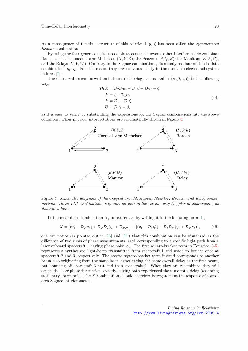
By using the four generators, it is possible to construct several other interferometric combina-tions, such as the unequal-arm Michelson (X, Y, Z), the Beacons (P,Q,R), the Monitors (E,F,G),and the Relays (U, V,W ). Contrary to the Sagnac combinations, these only use four of the six datacombinations ηi, η′i. For this reason they have obvious utility in the event of selected subsystemfailures [7].
These observables can be written in terms of the Sagnac observables (α, β, γ, ζ) in the followingway,
D1X = D2D3α−D2β −D3γ + ζ,
P = ζ −D1α,
E = D1 −D1ζ,
U = D1γ − β,
(44)
as it is easy to verify by substituting the expressions for the Sagnac combinations into the aboveequations. Their physical interpretations are schematically shown in Figure 5.
2
2
P,Q,R ( )Beacon
E,F,G ( )Monitor
2
2
3
3
1
1 1
1
3
3
X,Y,Z ( )Unequal−arm Michelson
Relay U,V,W ( )
Figure 5: Schematic diagrams of the unequal-arm Michelson, Monitor, Beacon, and Relay combi-nations. These TDI combinations rely only on four of the six one-way Doppler measurements, asillustrated here.
In the case of the combination X, in particular, by writing it in the following form [1],
X = [(η′1 +D2′η3) +D2′D2(η1 +D3η′2)]− [(η1 +D3η
′2) +D3D3′(η′1 +D2′η3)] , (45)
one can notice (as pointed out in [26] and [25]) that this combination can be visualized as thedifference of two sums of phase measurements, each corresponding to a specific light path from alaser onboard spacecraft 1 having phase noise φ1. The first square-bracket term in Equation (45)represents a synthesized light-beam transmitted from spacecraft 1 and made to bounce once atspacecraft 2 and 3, respectively. The second square-bracket term instead corresponds to anotherbeam also originating from the same laser, experiencing the same overall delay as the first beam,but bouncing off spacecraft 3 first and then spacecraft 2. When they are recombined they willcancel the laser phase fluctuations exactly, having both experienced the same total delay (assumingstationary spacecraft). The X combinations should therefore be regarded as the response of a zero-area Sagnac interferometer.
Living Reviews in Relativityhttp://www.livingreviews.org/lrr-2005-4

24 Massimo Tinto and Sanjeev V. Dhurandhar
5 Time-Delay Interferometry with Moving Spacecraft
The rotational motion of the LISA array results in a difference of the light travel times in the twodirections around a Sagnac circuit [24, 5]. Two time delays along each arm must be used, say L
′
i
and Li for clockwise or counter-clockwise propagation as they enter in any of the TDI combinations.Furthermore, since Li and L
′
i not only differ from one another but can be time dependent (they“flex”), it was shown that the “first generation” TDI combinations do not completely cancel thelaser phase noise (at least with present laser stability requirements), which can enter at a levelabove the secondary noises. For LISA, and assuming Li ' 10 m/s [13], the estimated magnitude ofthe remaining frequency fluctuations from the laser can be about 30 times larger than the level setby the secondary noise sources in the center of the frequency band. In order to solve this potentialproblem, it has been shown that there exist new TDI combinations that are immune to first ordershearing (flexing, or constant rate of change of delay times). These combinations can be derivedby using the time-delay operators formalism introduced in the previous Section 4, although onehas to keep in mind that now these operators no longer commute [34].
In order to derive the new, “flex-free” TDI combinations we will start by taking specific combi-nations of the one-way data entering in each of the expressions derived in the previous Section 4.These combinations are chosen in such a way so as to retain only one of the three noises φi,i = 1, 2, 3, if possible. In this way we can then implement an iterative procedure based on the useof these basic combinations and of time-delay operators, to cancel the laser noises after droppingterms that are quadratic in L/c or linear in the accelerations. This iterative time-delay method, tofirst order in the velocity, is illustrated abstractly as follows. Given a function of time Ψ = Ψ(t),time delay by Li is now denoted either with the standard comma notation [1] or by applying thedelay operator Di introduced in the previous Section 4,
DiΨ = Ψ,i ≡ Ψ(t− Li(t)). (46)
We then impose a second time delay Lj(t):
DjDiΨ = Ψ;ij ≡ Ψ(t− Lj(t)− Li(t− Lj(t)))
' Ψ(t− Lj(t)− Li(t) + Li(t)Lj)
' Ψ,ij + Ψ,ijLiLj . (47)
A third time delay Lk(t) gives
DkDjDiΨ = Ψ;ijk = Ψ(t− Lk(t)− Lj(t− Lk(t))− Li(t− Lk(t)− Lj(t− Lk(t))))
' Ψ,ijk + Ψ,ijk
[Li(Lj + Lk) + LjLk
], (48)
and so on, recursively; each delay generates a first-order correction proportional to its rate ofchange times the sum of all delays coming after it in the subscripts. Commas have now beenreplaced with semicolons [25], to remind us that we consider moving arrays. When the sum ofthese corrections to the terms of a data combination vanishes, the combination is called flex-free.
Also, note that each delay operator Di has a unique inverse D−1i , whose expression can be
derived by requiring that D−1i Di = I, and neglecting quadratic and higher order velocity terms.
Its action on a time series Ψ(t) is
D−1i Ψ(t) ≡ Ψ(t + Li(t + Li)). (49)
Note that this is not like an advance operator one might expect, since it advances not by Li(t) butrather Li(t + Li).
Living Reviews in Relativityhttp://www.livingreviews.org/lrr-2005-4

Time-Delay Interferometry 25
5.1 The unequal-arm Michelson
The unequal-arm Michelson combination relies on the four measurements η1, η1′ , η2′ , and η3.Note that the two combinations η1 + η2′,3, η1′ + η3,2′ represent the two synthesized two-way datameasured onboard spacecraft 1, and can be written in the following form,
η1 + η2′,3 = (D3D3′ − I) φ1, (50)η1′ + η3,2′ = (D2′D2 − I) φ1, (51)
where I is the identity operator. Since in the stationary case any pairs of these operators commute,i.e. DiDj′ −Dj′Di = 0, from Equations (50, 51) it is easy to derive the following expression for theunequal-arm interferometric combination X which eliminates φ1:
X = [D2′D2 − I] (η1 + η2′,3)− [(D3D3′ − I)] (η1′ + η3,2′). (52)
If, on the other hand, the time-delays depend on time, the expression of the unequal-arm Michelsoncombination above no longer cancels φ1. In order to derive the new expression for the unequal-arminterferometer that accounts for “flexing”, let us first consider the following two combinations ofthe one-way measurements entering into the X observable given in Equation (52):
[(η1′ + η3;2′) + (η1 + η2;3);22′ ] = [D2′D2D3D3′ − I]φ1, (53)[(η1 + η2′;3) + (η1′ + η3;2′);3′3] = [D3D3′D2′D2 − I]φ1. (54)
Using Equations (53, 54) we can use the delay technique again to finally derive the followingexpression for the new unequal-arm Michelson combination X1 that accounts for the flexing effect:
X1 = [D2D2′D3′D3 − I] [(η21 + η12;3′) + (η31 + η13;2);33′ ]− [D3′D3D2D2′ − I] [(η31 + η13;2) + (η21 + η12;3′);2′2] . (55)
As usual, X2 and X3 are obtained by cyclic permutation of the spacecraft indices. This expressionis readily shown to be laser-noise-free to first order of spacecraft separation velocities Li: it is“flex-free”.
5.2 The Sagnac combinations
In the above Section 5.1 we have used the same symbol X for the unequal-arm Michelson com-bination for both the rotating (i.e. constant delay times) and stationary cases. This emphasizesthat, for this TDI combination (and, as we will see below, also for all the combinations includingonly four links) the forms of the equations do not change going from systems at rest to the ro-tating case. One needs only distinguish between the time-of-flight variations in the clockwise andcounter-clockwise senses (primed and unprimed delays).
In the case of the Sagnac variables (α, β, γ, ζ), however, this is not the case as it is easy tounderstand on simple physical grounds. In the case of α for instance, light originating fromspacecraft 1 is simultaneously sent around the array on clockwise and counter-clockwise loops, andthe two returning beams are then recombined. If the array is rotating, the two beams experiencea different delay (the Sagnac effect), preventing the noise φ1 from cancelling in the α combination.
In order to find the solution to this problem let us first rewrite α in such a way to explicitlyemphasize what it does: attempts to remove the same fluctuations affecting two beams that havebeen made to propagated clockwise and counter-clockwise around the array,
α = [η1′ +D2′η3′ +D1′D2′η2′ ]− [η1 +D3η2 +D1D3η2], (56)
Living Reviews in Relativityhttp://www.livingreviews.org/lrr-2005-4

26 Massimo Tinto and Sanjeev V. Dhurandhar
where we have accounted for clockwise and counter-clockwise light delays. It is straight-forward toverify that this combination no longer cancels the laser and optical bench noises. If, however, weexpand the two terms inside the square-brackets on the right-hand side of Equation (56) we findthat they are equal to
[η1′ +D2′η3′ +D1′D2′η2′ ] = [D2′D1′D3′ − I]φ1 (57)[η1 +D3η2 +D1D3η2] = [D3D1D2 − I]φ1. (58)
If we now apply our iterative scheme to the combinations given in Equation (58) we finally get theexpression for the Sagnac combination α1 that is unaffected by laser noise in presence of rotation,
α1 = [D3D1D2 − I] [η1′ +D2′η3′ +D1′D2′η2′ ]− [D2′D1′D3′ − I] [η1 +D3η2 +D1D3η2]. (59)
If the delay-times are also time-dependent, we find that the residual laser noise remaining into thecombination α1 is actually equal to
φ1,1231′2′3′
[(L1 + L2 + L3
) (L
′
1 + L′
2 + L′
3
)−
(L
′
1 + L′
2 + L′
3
)(L1 + L2 + L3)
]. (60)
Fortunately, although first order in the relative velocities, the residual is small, as it involves thedifference of the clockwise and counter-clockwise rates of change of the propagation delays on thesame circuit. For LISA, the remaining laser phase noises in αi, i = 1, 2, 3, are several orders ofmagnitude below the secondary noises.
In the case of ζ, however, the rotation of the array breaks the symmetry and therefore itsuniqueness. However, there still exist three generalized TDI laser-noise-free data combinationsthat have properties very similar to ζ, and which can be used for the same scientific purposes [30].These combinations, which we call (ζ1, ζ2, ζ3), can be derived by applying again our time-delayoperator approach.Let us consider the following combination of the ηi, ηi′ measurements, each being delayed onlyonce [1]:
η3,3 − η3′,3 + η1,1′ = [D3D2 −D1′ ]φ1, (61)η1′,1 − η2,2′ + η2′,2′ = [D3′D2′ −D1]φ1, (62)
where we have used the commutativity property of the delay operators in order to cancel the φ2
and φ3 terms. Since both sides of the two equations above contain only the φ1 noise, ζ1 is foundby the following expression:
ζ1 = [D3′D2′ −D1] (η31,1′ − η32,2 + η12,2)− [D2D3 −D1′ ] (η13,3′ − η23,3′ + η21,1) . (63)
If the light-times in the arms are equal in the clockwise and counter-clockwise senses (e.g. norotation) there is no distinction between primed and unprimed delay times. In this case, ζ1 isrelated to our original symmetric Sagnac ζ by ζ1 = ζ,23 − ζ,1. Thus for the practical LISA case(arm length difference < 1%), the SNR of ζ1 will be the same as the SNR of ζ.
If the delay-times also change with time, the perfect cancellation of the laser noises is no longerachieved in the (ζ1, ζ2, ζ3) combinations. However, it has been shown in [34] that the magnitude ofthe residual laser noises in these combinations are significantly smaller than the LISA secondarysystem noises, making their effects entirely negligible.
The expressions for the Monitor, Beacon, and Relay combinations, accounting for the rotationand flexing of the LISA array, have been derived in the literature [34] by applying the time-delayiterative procedure highlighted in this section. The interested reader is referred to that paper fordetails.
Living Reviews in Relativityhttp://www.livingreviews.org/lrr-2005-4

Time-Delay Interferometry 27
A mathematical formulation of the “second generation” TDI, which generalizes the one pre-sented in Section 4 for the stationary LISA, still needs to be derived. In the case when only theSagnac effect is considered (and the delay-times remain constant in time) the mathematical for-mulation of Section 4 can be extended in a straight-forward way where now the six time-delaysDi and D′i must be taken into account. The polynomial ring is now in these six variables andthe corresponding module of syzygies can be constructed over this enlarged polynomial ring [22].However, when the arms are allowed to flex, that is, the operators themselves are functions oftime, the operators no longer commute. One must then resort to non-commutative Grobner basismethods. We will investigate this mathematical problem in the near future.
Living Reviews in Relativityhttp://www.livingreviews.org/lrr-2005-4

28 Massimo Tinto and Sanjeev V. Dhurandhar
6 Optimal LISA Sensitivity
All the above interferometric combinations have been shown to individually have rather differentsensitivities [7], as a consequence of their different responses to gravitational radiation and systemnoises. Since LISA has the capability of simultaneously observing a gravitational wave signal withmany different interferometric combinations (all having different antenna patterns and noises), weshould no longer regard LISA as a single detector system but rather as an array of gravitationalwave detectors working in coincidence. This suggests that the presently adopted LISA sensitivitycould be improved by optimally combining elements of the TDI space.
Before proceeding with this idea, however, let us consider again the so-called “second gen-eration” TDI Sagnac observables: (α1, α2, α3). The expressions of the gravitational wave signaland the secondary noise sources entering into α1 will in general be different from those enteringinto α, the corresponding Sagnac observable derived under the assumption of a stationary LISAarray [1, 7]. However, the other remaining, secondary noises in LISA are so much smaller, andthe rotation and systematic velocities in LISA are so intrinsically small, that index permutationmay still be done for them [34]. It is therefore easy to derive the following relationship betweenthe signal and secondary noises in α1, and those entering into the stationary TDI combinationα [25, 34],
α1(t) ' α(t)− α(t− L1 − L2 − L3), (64)
where Li, i = 1, 2, 3, are the unequal-arm lengths of the stationary LISA array. Equation (64)implies that any data analysis procedure and algorithm that will be implemented for the second-generation TDI combinations can actually be derived by considering the corresponding “first gen-eration” TDI combinations. For this reason, from now on we will focus our attention on thegravitational wave responses of the first-generation TDI observables (α, β, γ, ζ).
As a consequence of these considerations, we can still regard (α, β, γ, ζ) as the generators ofthe TDI space, and write the most general expression for an element of the TDI space, η(f), as alinear combination of the Fourier transforms of the four generators (α, β, γ, ζ),
η(f) ≡ a1(f,~λ) α(f) + a2(f,~λ) β(f) + a3(f,~λ) γ(f) + a4(f,~λ) ζ(f), (65)
where the {ai(f,~λ)}4i=1 are arbitrary complex functions of the Fourier frequency f , and of avector ~λ containing parameters characterizing the gravitational wave signal (source location in thesky, waveform parameters, etc.) and the noises affecting the four responses (noise levels, theircorrelations, etc.). For a given choice of the four functions {ai}4i=1, η gives an element of thefunctional space of interferometric combinations generated by (α, β, γ, ζ). Our goal is thereforeto identify, for a given gravitational wave signal, the four functions {ai}4i=1 that maximize thesignal-to-noise ratio SNR2
η of the combination η,
SNR2η =
∫ fu
fl
∣∣∣a1 αs + a2 βs + a3 γs + a4ζs
∣∣∣2⟨∣∣∣a1 αn + a2 βn + a3 γn + a4 ζn
∣∣∣2⟩ df. (66)
In Equation (66) the subscripts s and n refer to the signal and the noise parts of (α, β, γ, ζ),respectively, the angle brackets represent noise ensemble averages, and the interval of integration(fl, fu) corresponds to the frequency band accessible by LISA.
Before proceeding with the maximization of the SNR2η we may notice from Equation (43) that
the Fourier transform of the totally symmetric Sagnac combination, ζ, multiplied by the transferfunction 1−e2πif(L1+L2+L3) can be written as a linear combination of the Fourier transforms of theremaining three generators (α, β, γ). Since the signal-to-noise ratio of η and (1−e2πif(L1+L2+L3))η
Living Reviews in Relativityhttp://www.livingreviews.org/lrr-2005-4

Time-Delay Interferometry 29
are equal, we may conclude that the optimization of the signal-to-noise ratio of η can be performedonly on the three observables α, β, γ. This implies the following redefined expression for SNR2
η:
SNR2η =
∫ fu
fl
∣∣∣a1 αs + a2 βs + a3 γs
∣∣∣2⟨∣∣∣a1 αn + a2 βn + a3 γn
∣∣∣2⟩ df. (67)
The SNR2η can be regarded as a functional over the space of the three complex functions {ai}3i=1,
and the particular set of complex functions that extremize it can of course be derived by solvingthe associated set of Euler–Lagrange equations.
In order to make the derivation of the optimal SNR easier, let us first denote by x(s) and x(n)
the two vectors of the signals (αs, βs, γs) and the noises (αn, βn, γn), respectively. Let us also definea to be the vector of the three functions {ai}3i=1, and denote with C the Hermitian, non-singular,correlation matrix of the vector random process xn,
(C)rt ≡⟨x(n)
r x(n)∗t
⟩. (68)
If we finally define (A)ij to be the components of the Hermitian matrix x(s)i x(s)∗
j , we can rewriteSNR2
η in the following form,
SNR2η =
∫ fu
fl
aiAija∗jarCrta∗t
df, (69)
where we have adopted the usual convention of summation over repeated indices. Since the noisecorrelation matrix C is non-singular, and the integrand is positive definite or null, the stationaryvalues of the signal-to-noise ratio will be attained at the stationary values of the integrand, whichare given by solving the following set of equations (and their complex conjugated expressions):
∂
∂ak
[aiAija∗jarCrta∗t
]= 0, k = 1, 2, 3. (70)
After taking the partial derivatives, Equation (70) can be rewritten in the following form,
(C−1)ir (A)rj (a∗)j =[
apApqa∗qalClma∗m
](a∗)i, i = 1, 2, 3, (71)
which tells us that the stationary values of the signal-to-noise ratio of η are equal to the eigenvaluesof the the matrix C−1 ·A. The result in Equation (70) is well known in the theory of quadraticforms, and it is called Rayleigh’s principle [18, 23].
In order now to identify the eigenvalues of the matrix C−1 ·A, we first notice that the 3 × 3matrix A has rank 1. This implies that the matrix C−1 ·A has also rank 1, as it is easy to verify.Therefore two of its three eigenvalues are equal to zero, while the remaining non-zero eigenvaluerepresents the solution we are looking for.
The analytic expression of the third eigenvalue can be obtained by using the property that thetrace of the 3 × 3 matrix C−1 ·A is equal to the sum of its three eigenvalues, and in our case tothe eigenvalue we are looking for. From these considerations we derive the following expression forthe optimized signal-to-noise ratio SNR2
η opt:
SNR2η opt =
∫ fu
fl
x(s)∗i (C−1)ij x(s)
j df. (72)
We can summarize the results derived in this section, which are given by Equations (67, 72), inthe following way:
Living Reviews in Relativityhttp://www.livingreviews.org/lrr-2005-4

30 Massimo Tinto and Sanjeev V. Dhurandhar
1. Among all possible interferometric combinations LISA will be able to synthesize with its fourgenerators α, β, γ, ζ, the particular combination giving maximum signal-to-noise ratio canbe obtained by using only three of them, namely (α, β, γ).
2. The expression of the optimal signal-to-noise ratio given by Equation (72) implies that LISAshould be regarded as a network of three interferometer detectors of gravitational radiation(of responses (α, β, γ)) working in coincidence [12, 21].
6.1 General application
As an application of Equation (72), here we calculate the sensitivity that LISA can reach when ob-serving sinusoidal signals uniformly distributed on the celestial sphere and of random polarization.In order to calculate the optimal signal-to-noise ratio we will also need to use a specific expressionfor the noise correlation matrix C. As a simplification, we will assume the LISA arm lengths tobe equal to their nominal value L = 16.67 s, the optical-path noises to be equal and uncorrelatedto each other, and finally the noises due to the proof-mass noises to be also equal, uncorrelated toeach other and to the optical-path noises. Under these assumptions the correlation matrix becomesreal, its three diagonal elements are equal, and all the off-diagonal terms are equal to each other,as it is easy to verify by direct calculation [7]. The noise correlation matrix C is therefore uniquelyidentified by two real functions Sα and Sαβ in the following way:
C =
Sα Sαβ Sαβ
Sαβ Sα Sαβ
Sαβ Sαβ Sα
. (73)
The expression of the optimal signal-to-noise ratio assumes a rather simple form if we diag-onalize this correlation matrix by properly “choosing a new basis”. There exists an orthogonaltransformation of the generators (α, β, γ) which will transform the optimal signal-to-noise ratiointo the sum of the signal-to-noise ratios of the “transformed” three interferometric combinations.The expressions of the three eigenvalues {µi}3i=1 (which are real) of the noise correlation matrixC can easily be found by using the algebraic manipulator Mathematica, and they are equal to
µ1 = µ2 = Sα − Sαβ , µ3 = Sα + 2Sαβ . (74)
Note that two of the three real eigenvalues, (µ1, µ2), are equal. This implies that the eigenvectorassociated to µ3 is orthogonal to the two-dimensional space generated by the eigenvalue µ1, whileany chosen pair of eigenvectors corresponding to µ1 will not necessarily be orthogonal. Thisinconvenience can be avoided by choosing an arbitrary set of vectors in this two-dimensional space,and by ortho-normalizing them. After some simple algebra, we have derived the following threeortho-normalized eigenvectors:
v1 =1√2
(−1, 0, 1) v2 =1√6
(1,−2, 1) v3 =1√3
(1, 1, 1). (75)
Equation (75) implies the following three linear combinations of the generators (α, β, γ):
A =1√2
(γ − α) E =1√6
(α− 2β + γ
)T =
1√3
(α + β + γ
), (76)
where A, E, and T are italicized to indicate that these are “orthogonal modes”. Although theexpressions for the modes A and E depend on our particular choice for the two eigenvectors(v1,v2), it is clear from our earlier considerations that the value of the optimal signal-to-noiseratio is unaffected by such a choice. From Equation (76) it is also easy to verify that the noise
Living Reviews in Relativityhttp://www.livingreviews.org/lrr-2005-4

Time-Delay Interferometry 31
correlation matrix of these three combinations is diagonal, and that its non-zero elements areindeed equal to the eigenvalues given in Equation (74).
In order to calculate the sensitivity corresponding to the expression of the optimal signal-to-noise ratio, we have proceeded similarly to what was done in [1, 7], and described in moredetail in [32]. We assume an equal-arm LISA (L = 16.67 s), and take the one-sided spectra ofproof mass and aggregate optical-path-noises (on a single link), expressed as fractional frequencyfluctuation spectra, to be Sproof mass
y = 2.5 × 10−48[f/1 Hz]−2 Hz−1 and Soptical pathy = 1.8 ×
10−37[f/1 Hz]2 Hz−1, respectively (see [7, 3]). We also assume that aggregate optical path noisehas the same transfer function as shot noise.
The optimum SNR is the square root of the sum of the squares of the SNRs of the three“orthogonal modes” (A,E, T ). To compare with previous sensitivity curves of a single LISAMichelson interferometer, we construct the SNRs as a function of Fourier frequency for sinusoidalwaves from sources uniformly distributed on the celestial sphere. To produce the SNR of each ofthe (A,E, T ) modes we need the gravitational wave response and the noise response as a functionof Fourier frequency. We build up the gravitational wave responses of the three modes (A,E, T )from the gravitational wave responses of (α, β, γ). For 7000 Fourier frequencies in the ∼ 10−4 Hzto ∼ 1 Hz LISA band, we produce the Fourier transforms of the gravitational wave response of(α, β, γ) from the formulas in [1, 32]. The averaging over source directions (uniformly distributedon the celestial sphere) and polarization states (uniformly distributed on the Poincare sphere) isperformed via a Monte Carlo method. From the Fourier transforms of the (α, β, γ) responses ateach frequency, we construct the Fourier transforms of (A,E, T ). We then square and average tocompute the mean-squared responses of (A,E, T ) at that frequency from 104 realizations of (sourceposition, polarization state) pairs.
We adopt the following terminology: We refer to a single element of the module as a datacombination, while a function of the elements of the module, such as taking the maximum overseveral data combinations in the module or squaring and adding data combinations belonging tothe module, is called as an observable. The important point to note is that the laser frequencynoise is also suppressed for the observable although it may not be an element of the module.
The noise spectra of (A,E, T ) are determined from the raw spectra of proof-mass and optical-path noises, and the transfer functions of these noises to (A,E, T ). Using the transfer functionsgiven in [7], the resulting spectra are equal to
SA(f) = SE(f) = 16 sin2(πfL) [3 + 2 cos(2πfL) + cos(4πfL)]Sproof massy (f)
+ 8 sin2(πfL) [2 + cos(2πfL)]Soptical pathy (f), (77)
ST (f) = 2[1 + 2 cos(2πfL)]2[4 sin2(πfL) Sproof mass
y + Soptical pathy (f)
]. (78)
Let the amplitude of the sinusoidal gravitational wave be h. The SNR for, e.g. A, SNRA, at eachfrequency f is equal to h times the ratio of the root-mean-squared gravitational wave responseat that frequency divided by
√SA(f) B, where B is the bandwidth conventionally taken to be
equal to 1 cycle per year. Finally, if we take the reciprocal of SNRA/h and multiply it by 5to get the conventional SNR = 5 sensitivity criterion, we obtain the sensitivity curve for thiscombination which can then be compared against the corresponding sensitivity curve for the equal-arm Michelson interferometer.
In Figure 6 we show the sensitivity curve for the LISA equal-arm Michelson response (SNR = 5)as a function of the Fourier frequency, and the sensitivity curve from the optimum weighting of the
data described above: 5h/√
SNR2A + SNR2
E + SNR2T . The SNRs were computed for a bandwidth of
1 cycle/year. Note that at frequencies where the LISA Michelson combination has best sensitivity,the improvement in signal-to-noise ratio provided by the optimal observable is slightly larger than√
2.
Living Reviews in Relativityhttp://www.livingreviews.org/lrr-2005-4

32 Massimo Tinto and Sanjeev V. Dhurandhar
Figure 6: The LISA Michelson sensitivity curve (SNR = 5) and the sensitivity curve for the optimalcombination of the data, both as a function of Fourier frequency. The integration time is equal toone year, and LISA is assumed to have a nominal armlength L = 16.67 s.
Figure 7: The optimal SNR divided by the SNR of a single Michelson interferometer, as a functionof the Fourier frequency f . The sensitivity gain in the low-frequency band is equal to
√2, while
it can get larger than 2 at selected frequencies in the high-frequency region of the accessible band.The integration time has been assumed to be one year, and the proof mass and optical path noisespectra are the nominal ones. See the main body of the paper for a quantitative discussion of thispoint.
Living Reviews in Relativityhttp://www.livingreviews.org/lrr-2005-4
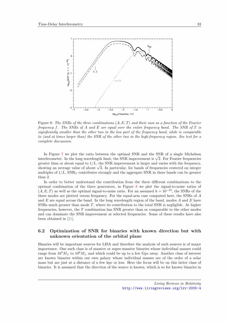
Time-Delay Interferometry 33
Figure 8: The SNRs of the three combinations (A,E, T ) and their sum as a function of the Fourierfrequency f . The SNRs of A and E are equal over the entire frequency band. The SNR of T issignificantly smaller than the other two in the low part of the frequency band, while is comparableto (and at times larger than) the SNR of the other two in the high-frequency region. See text for acomplete discussion.
In Figure 7 we plot the ratio between the optimal SNR and the SNR of a single Michelsoninterferometer. In the long-wavelength limit, the SNR improvement is
√2. For Fourier frequencies
greater than or about equal to 1/L, the SNR improvement is larger and varies with the frequency,showing an average value of about
√3. In particular, for bands of frequencies centered on integer
multiples of 1/L, SNRT contributes strongly and the aggregate SNR in these bands can be greaterthan 2.
In order to better understand the contribution from the three different combinations to theoptimal combination of the three generators, in Figure 8 we plot the signal-to-noise ratios of(A,E, T ) as well as the optimal signal-to-noise ratio. For an assumed h = 10−23, the SNRs of thethree modes are plotted versus frequency. For the equal-arm case computed here, the SNRs of Aand E are equal across the band. In the long wavelength region of the band, modes A and E haveSNRs much greater than mode T , where its contribution to the total SNR is negligible. At higherfrequencies, however, the T combination has SNR greater than or comparable to the other modesand can dominate the SNR improvement at selected frequencies. Some of these results have alsobeen obtained in [21].
6.2 Optimization of SNR for binaries with known direction but withunknown orientation of the orbital plane
Binaries will be important sources for LISA and therefore the analysis of such sources is of majorimportance. One such class is of massive or super-massive binaries whose individual masses couldrange from 103M� to 108M� and which could be up to a few Gpc away. Another class of interestare known binaries within our own galaxy whose individual masses are of the order of a solarmass but are just at a distance of a few kpc or less. Here the focus will be on this latter class ofbinaries. It is assumed that the direction of the source is known, which is so for known binaries in
Living Reviews in Relativityhttp://www.livingreviews.org/lrr-2005-4

34 Massimo Tinto and Sanjeev V. Dhurandhar
our galaxy. However, even for such binaries, the inclination angle of the plane of the orbit of thebinary is either poorly estimated or unknown. The optimization problem is now posed differently:The SNR is optimized after averaging over the polarizations of the binary signals, so the resultsobtained are optimal on the average, that is, the source is tracked with an observable which isoptimal on the average [21]. For computing the average, a uniform distribution for the directionof the orbital angular momentum of the binary is assumed.
When the binary masses are of the order of a solar mass and the signal typically has a frequencyof a few mHz, the GW frequency of the binary may be taken to be constant over the period ofobservation, which is typically taken to be of the order of an year. A complete calculation of thesignal matrix and the optimization procedure of SNR is given in [20]. Here we briefly mention themain points and the final results.
A source fixed in the Solar System Barycentric reference frame in the direction (θB, φB) isconsidered. But as the LISA constellation moves along its heliocentric orbit, the apparent direction(θL, φL) of the source in the LISA reference frame (xL, yL, zL) changes with time. The LISAreference frame (xL, yL, zL) has been defined in [20] as follows: The origin lies at the center ofthe LISA triangle and the plane of LISA coincides with the (xL, yL) plane with spacecraft 2 lyingon the xL axis. Figure (9) displays this apparent motion for a source lying in the ecliptic plane,that is with θB = 90◦ and φB = 0◦. The source in the LISA reference frame describes a figure of8. Optimizing the SNR amounts to tracking the source with an optimal observable as the sourceapparently moves in the LISA reference frame.
-1
-0.5 0
0.5 1
x L
-1 -0.5 0 0.5 1y L
-1
-0.5
0
0.5
1
z L
Figure 9: Apparent position of the source in the sky as seen from LISA frame for (θB = 90◦, φB =0◦). The track of the source for a period of one year is shown on the unit sphere in the LISAreference frame.
Since an average has been taken over the orientation of the orbital plane of the binary or equiv-alently over the polarizations, the signal matrix A is now of rank 2 instead of rank 1 as comparedwith the application in the previous Section 6.1. The mutually orthogonal data combinations A,E, T are convenient in carrying out the computations because in this case as well, they simulta-neously diagonalize the signal and the noise covariance matrix. The optimization problem nowreduces to an eigenvalue problem with the eigenvalues being the squares of the SNRs. There aretwo eigen-vectors which are labelled as ~v+,× belonging to two non-zero eigenvalues. The two SNRs
Living Reviews in Relativityhttp://www.livingreviews.org/lrr-2005-4

Time-Delay Interferometry 35
are labelled as SNR+ and SNR×, corresponding to the two orthogonal (thus statistically indepen-dent) eigen-vectors ~v+,×. As was done in the previous Section 6.1 F the two SNRs can be squaredand added to yield a network SNR, which is defined through the equation
SNR2network = SNR2
+ + SNR2×. (79)
The corresponding observable is called the network observable. The third eigenvalue is zero andthe corresponding eigenvector orthogonal to ~v+ and ~v× gives zero signal.
The eigenvectors and the SNRs are functions of the apparent source direction parameters(θL, φL) in the LISA reference frame, which in turn are functions of time. The eigenvectors opti-mally track the source as it moves in the LISA reference frame. Assuming an observation period ofan year, the SNRs are integrated over this period of time. The sensitivities are computed accordingto the procedure described in the previous Section 6.1. The results of these findings are displayedin Figure 10.
It shows the sensitivity curves of the following observables:
1. The Michelson combination X (faint solid curve).
2. The observable obtained by taking the maximum sensitivity among X, Y , and Z for eachdirection, where Y and Z are the Michelson observables corresponding to the remaining twopairs of arms of LISA [1]. This maximum is denoted by max[X, Y, Z] (dash-dotted curve)and is operationally given by switching the combinations X, Y , Z so that the best sensitivityis achieved.
3. The eigen-combination ~v+ which has the best sensitivity among all data combinations (dashedcurve).
4. The network observable (solid curve).
It is observed that the sensitivity over the band-width of LISA increases as one goes fromObservable 1 to 4. Also it is seen that the max[X, Y, Z] does not do much better than X. This isbecause for the source direction chosen θB = 90◦, X is reasonably well oriented and switching toY and Z combinations does not improve the sensitivity significantly. However, the network and~v+ observables show significant improvement in sensitivity over both X and max[X, Y, Z]. This isthe typical behavior and the sensitivity curves (except X) do not show much variations for othersource directions and the plots are similar. Also it may be fair to compare the optimal sensitivitieswith max[X, Y, Z] rather than X. This comparison of sensitivities is shown in Figure 11, wherethe network and the eigen-combinations ~v+,× are compared with max[X, Y, Z].
Defining
κa(f) =SNRa(f)
SNRmax[X,Y,Z](f), (80)
where the subscript a stands for network or +, ×, and SNRmax[X,Y,Z] is the SNR of the observablemax[X, Y, Z], the ratios of sensitivities are plotted over the LISA band-width. The improvementin sensitivity for the network observable is about 34% at low frequencies and rises to nearly 90%at about 20 mHz, while at the same time the ~v+ combination shows improvement of 12% at lowfrequencies rising to over 50% at about 20 mHz.
Living Reviews in Relativityhttp://www.livingreviews.org/lrr-2005-4

36 Massimo Tinto and Sanjeev V. Dhurandhar
10-24
10-23
10-22
10-21
10-20
10-4 10-3 10-2 10-1
Sen
sitiv
ity
Frequency in Hz
Eigen-observable V+Network observable
Michelson XMax[X,Y,Z]
Figure 10: Sensitivity curves for the observables: Michelson, max[X, Y, Z], ~v+, and network forthe source direction (θB = 90◦, φB = 0◦).
0.5
1
1.5
2
10-4 10-3 10-2 10-1
SN
R R
atio
s κ
Frequency in Hz
κnetworkκ+κx
Figure 11: Ratios of the sensitivities of the observables network, ~v+,× with max[X, Y, Z] for thesource direction θB = 90◦, φB = 0◦.
Living Reviews in Relativityhttp://www.livingreviews.org/lrr-2005-4

Time-Delay Interferometry 37
7 Concluding Remarks
In this article we have summarized the use of TDI for canceling the laser phase noise from het-erodyne phase measurements performed by a constellation of three spacecraft tracking each otheralong arms of unequal length. Underlying the TDI technique is the mathematical structure ofthe theory of Grobner basis and the algebra of modules over polynomial rings. These methodshave been motivated and illustrated with the simple example of an unequal-arm interferometerin order to give a physical insight of TDI. Here, these methods have been rigorously applied tothe idealized case of a stationary LISA for deriving the generators of the module from which theentire TDI data set can be obtained; they can be extended in a straight-forward way to morethan three spacecraft for possible LISA follow-on missions. The stationary LISA case was used asa propaedeutical introduction to the physical motivation of TDI, and for further extending it tothe realistic LISA configuration of free-falling spacecraft orbiting around the Sun. The TDI datacombinations canceling laser phase noise in this general case are referred to as second generationTDI, and they contain twice as many terms as their corresponding first generation combinationsvalid for the stationary configuration.
As a data analysis application we have shown that it is possible to identify specific TDI combi-nations that will allow LISA to achieve optimal sensitivity to gravitational radiation [19, 21, 20].The resulting improvement in sensitivity over that of an unequal-arm Michelson interferometer, inthe case of monochromatic signals randomly distributed over the celestial sphere and of randompolarization, is non-negligible. We have found this to be equal to a factor of
√2 in the low-part of
the frequency band, and slightly more than√
3 in the high-part of the LISA band. The SNR forbinaries whose location in the sky is known, but their polarization is not, can also be optimized,and the degree of improvement depends on the location of the source in the sky.
As a final remark we would like to emphasize that this field of research, TDI, is still very youngand evolving. Possible physical phenomena, yet unrecognized, might turn out to be importantto account for within the TDI framework. The purpose of this review was to provide the basicmathematical tools needed for working on future TDI projects. We hope to have accomplishedthis goal, and that others will be stimulated to work in this new and fascinating field of research.
Living Reviews in Relativityhttp://www.livingreviews.org/lrr-2005-4

38 Massimo Tinto and Sanjeev V. Dhurandhar
8 Acknowledgement
S.V.D. acknowledges support from IFCPAR, Delhi, India under which the work was carried outin collaboration with J.-Y. Vinet. This research was performed at the Jet Propulsion Labora-tory, California Institute of Technology, under contract with the National Aeronautics and SpaceAdministration.
Living Reviews in Relativityhttp://www.livingreviews.org/lrr-2005-4

Time-Delay Interferometry 39
A Generators of the Module of Syzygies
We require the 4-tuple solutions (q3, q′1, q
′2, q
′3) to the equation
(1− xyz) q3 + (xz − y) q′1 + x(1− z2) q′2 + (1− x2) q′3 = 0, (81)
where for convenience we have substituted x = D1, y = D2, z = D3. q3, q′1, q′2, q′3 are polynomialsin x, y, z with integral coefficients, i.e. in Z[x, y, z].
We now follow the procedure in the book by Becker et al. [2].Consider the ideal in Z[x, y, z] (or Q[x, y, z] where Q denotes the field of rational numbers),
formed by taking linear combinations of the coefficients in Equation (81), f1 = 1−xyz, f2 = xz−y,f3 = x(1− z2), f4 = 1− x2. A Grobner basis for this ideal is
G = {g1 = z2 − 1, g2 = y2 − 1, g3 = x− yz}. (82)
The above Grobner basis is obtained using the function GroebnerBasis in Mathematica. One cancheck that both the fi, i = 1, 2, 3, 4, and gj , j = 1, 2, 3, generate the same ideal because we canexpress one generating set in terms of the other and vice-versa:
fi = dijgj , gj = cjifi, (83)
where d and c are 4× 3 and 3× 4 polynomial matrices, respectively, and are given by
d =
−1 −z2 −yzy 0 z−x 0 0−1 −z2 −(x + yz)
, c =
0 0 −x z2 − 1−1 −y 0 00 z 1 0
. (84)
The generators of the 4-tuple module are given by the set A⋃
B∗, where A and B∗ are the setsdescribed below:
A is the set of row vectors of the matrix I −d · c where the dot denotes the matrix product andI is the identity matrix, 4× 4 in our case. Thus,
a1 =(z2 − 1, 0, x− yz, 1− z2
),
a2 =(0, z
(1− z2
), xy − z, y
(1− z2
)),
a3 =(0, 0, 1− x2, x
(z2 − 1
)),
a4 =(−z2, xz, yz, z2
).
(85)
We thus first get 4 generators. The additional generators are obtained by computing the S-polynomials of the Grobner basis G. The S-polynomial of two polynomials g1, g2 is obtained bymultiplying g1 and g2 by suitable terms and then adding, so that the highest terms cancel. Forexample in our case g1 = z2 − 1 and g2 = y2 − 1, and the highest terms are z2 for g1 and y2 forg2. Multiply g1 by y2 and g2 by z2 and subtract. Thus, the S-polynomial p12 of g1 and g2 is
p12 = y2g1 − z2g2 = z2 − y2. (86)
Note that order is defined (x � y � z) and the y2z2 term cancels. For the Grobner basis of3 elements we get 3 S-polynomials p12, p13, p23. The pij must now be re-expressed in terms ofthe Grobner basis G. This gives a 3 × 3 matrix b. The final step is to transform to 4-tuples bymultiplying b by the matrix c to obtain b∗ = b · c. The row vectors b∗i , i = 1, 2, 3, of b∗ form theset B∗:
b∗1 =(z2 − 1, y
(z2 − 1
), x
(1− y2
),(y2 − 1
) (z2 − 1
)),
b∗2 =(0, z
(1− z2
), 1− z2 − x (x− yz) , (x− yz)
(z2 − 1
)),
b∗3 =(−x + yz, z − xy, 1− y2, 0
).
(87)
Thus we obtain 3 more generators which gives us a total of 7 generators of the required module ofsyzygies.
Living Reviews in Relativityhttp://www.livingreviews.org/lrr-2005-4

40 Massimo Tinto and Sanjeev V. Dhurandhar
B Conversion between Generating Sets
We list the three sets of generators and relations among them. We first list below α, β, γ, ζ:
α = (−1,−z,−xz, 1, xy, y),β = (−xy,−1,−x, z, 1, yz),γ = (−y,−yz,−1, xz, x, 1),ζ = (−x,−y,−z, x, y, z).
(88)
We now express the ai and b∗j in terms of α, β, γ, ζ:
a1 = γ − zζ,
a2 = α− zβ,
a3 = −zα + β − xγ + xzζ,
a4 = zζ,
b∗1 = −yα + yzβ + γ − zζ,
b∗2 = (1− z2)β − xγ + xzζ,
b∗3 = β − yζ.
(89)
Further we also list below α, β, γ, ζ in terms of X(A):
α = X(3),
β = X(4),
γ = −X(1) + zX(2),
ζ = X(2).
(90)
This proves that since the ai, b∗j generate the required module, the α, β, γ, ζ and X(A), A = 1, 2, 3, 4,also generate the same module.
The Grobner basis is given in terms of the above generators as follows: G(1) = ζ, G(2) = X(1),G(3) = β, G(4) = α, and G(5) = a3.
Living Reviews in Relativityhttp://www.livingreviews.org/lrr-2005-4

Time-Delay Interferometry 41
References
[1] Armstrong, J.W., Estabrook, F.B., and Tinto, M., “Time-Delay Interferometry for Space-based Gravitational Wave Searches”, Astrophys. J., 527, 814–826, (1999). 1, 3, 4.3, 4.7, 4.7,5, 5.2, 6, 6.1, 2
[2] Becker, T., and Weispfenning, V., Grobner Bases: A Computational Approach to Commuta-tive Algebra, vol. 141 of Graduate Texts in Mathematics, (Springer, Berlin, Germany; NewYork, U.S.A., 1993). 1, 4.3, 4.4, 4.5, A
[3] Bender, P.L., Brillet, A., Ciufolini, I., Cruise, A.M., Cutler, C., Danzmann, K., Fidecaro, F.,Folkner, W.M., Hough, J., McNamara, P.W., Peterseim, M., Robertson, D., Rodrigues, M.,Rudiger, A., Sandford, M., Schafer, G., Schilling, R., Schutz, B.F., Speake, C.C., Stebbins,R.T., Sumner, T.J., Touboul, P., Vinet, J.-Y., Vitale, S., Ward, H., and Winkler, W. (LISAStudy Team), LISA. Laser Interferometer Space Antenna for the detection and observationof gravitational waves. An international project in the field of Fundamental Physics in Space.Pre-Phase A report, MPQ-233, (Max-Planck-Institut fur Quantenoptik, Garching, Germany,1998). Related online version (cited on 06 July 2005):ftp://ftp.ipp-garching.mpg.de/pub/grav/lisa/pdd/. 1, 2, 6.1
[4] Bender, P.L., and Hils, D., “Confusion noise level due to galactic and extragalactic binaries”,Class. Quantum Grav., 14, 1439–1444, (1997). 1
[5] Cornish, N.J., and Hellings, R.W., “The effects of orbital motion on LISA time delay inter-ferometry”, Class. Quantum Grav., 20, 4851–4860, (2003). 1, 3, 3, 5
[6] Dhurandhar, S.V., Rajesh Nayak, K., and Vinet, J.Y., “Algebraic approach to time-delaydata analysis for LISA”, Phys. Rev. D, 65, 102002–1–16, (2002). 1
[7] Estabrook, F.B., Tinto, M., and Armstrong, J.W., “Time-delay analysis of LISA gravitationalwave data: Elimination of spacecraft motion effects”, Phys. Rev. D, 62, 042002–1–8, (2000).1, 3, 3, 3, 4.3, 4.7, 6, 6.1, 6.1
[8] Estabrook, F.B., and Wahlquist, H.D., “Response of Doppler spacecraft tracking to gravita-tional radiation”, Gen. Relativ. Gravit., 6, 439–447, (1975). 1
[9] Faller, J.E., and Bender, P.L., “A possible laser gravitational wave experiment in space”, inTaylor, B.N., and Phillips, W.D., eds., Precision Measurement and Fundamental Constants II,Proceedings of the Second International Conference held at the National Bureau of Standards,Gaithersburg, MD, June 8–12, 1981, vol. 617 of NBS Special Publication, 689–690, (U.S. Dept.of Commerce / National Bureau of Standards, Washington, U.S.A., 1984). 2, 2
[10] Faller, J.E., Bender, P.L., Hall, J.L., Hils, D., Stebbins, R.T., and Vincent, M.A., “An antennafor laser gravitational-wave observations in space”, Adv. Space Res., 9(9), 107–111, (1989).COSPAR and IAU, 27th Plenary Meeting, 15th Symposium on Relativistic Gravitation, Es-poo, Finland, July 18–29, 1988. 2
[11] Faller, J.E., Bender, P.L., Hall, J.L., Hils, D., and Vincent, M.A., “Space antenna for grav-itational wave astronomy”, in Longdon, N., and Melita, O., eds., Kilometric Optical Arraysin Space, Proceedings of the Colloquium held 23–25 October 1984, Cargese, Corsica, France,vol. SP-226 of ESA Conference Proceedings, 157–163, (ESA Publications Division, Noordwijk,Netherlands, 1985). 2
[12] Finn, L.S., “Aperture synthesis for gravitational-wave data analysis: Deterministic sources”,Phys. Rev. D, 63, 102001–1–18, (2001). 2
Living Reviews in Relativityhttp://www.livingreviews.org/lrr-2005-4

42 Massimo Tinto and Sanjeev V. Dhurandhar
[13] Folkner, W.M., Hechler, F., Sweetser, T.H., Vincent, M.A., and Bender, P.L., “LISA orbitselection and stability”, Class. Quantum Grav., 14, 1405–1410, (1997). 5
[14] Giampieri, G., Hellings, R.W., Tinto, M., and Faller, J.E., “Algorithms for unequal-armMichelson interferometers”, Opt. Commun., 123, 669–678, (1996). 2
[15] Jenkins, G.M., and Watts, D.G., Spectral Analysis and its Applications, (Holden-Day, SanFrancisco, U.S.A., 1968). 2
[16] Kreuzer, M., and Robbiano, L., Computational Commutative Algebra 1, (Springer, Berlin,Germany; New York, U.S.A., 2000). 1, 4.3, 4.5
[17] Nelemans, G., Yungelson, L.R., and Portegies Zwart, S.F., “The gravitational wave signal fromthe Galactic disk population of binaries containing two compact objects”, Astron. Astrophys.,375, 890–898, (2001). 1
[18] Noble, B., Applied Linear Algebra, (Prentice-Hall, Englewood Cliffs, U.S.A., 1969). 6
[19] Prince, T.A., Tinto, M., Larson, S.L., and Armstrong, J.W., “LISA optimal sensitivity”, Phys.Rev. D, 66, 122002–1–7, (2002). 1, 7
[20] Rajesh Nayak, K., Dhurandhar, S.V., Pai, A., and Vinet, J.-Y., “Optimizing the directionalsensitivity of LISA”, Phys. Rev. D, 68, 122001–1–11, (2003). 1, 6.2, 7
[21] Rajesh Nayak, K., Pai, A., Dhurandhar, S.V., and Vinet, J.-Y., “Improving the sensitivity ofLISA”, Class. Quantum Grav., 20, 1217–1231, (2003). 1, 2, 6.1, 6.2, 7
[22] Rajesh Nayak, K., and Vinet, J.-Y., unknown status. In preparation. 5.2
[23] Selby, S.M., Standard of Mathematical Tables, (The Chemical Rubber Co., Cleveland, U.S.A.,1964). 6
[24] Shaddock, D.A., “Operating LISA as a Sagnac interferometer”, Phys. Rev. D, 69, 022001–1–6,(2004). 1, 3, 5
[25] Shaddock, D.A., Tinto, M., Estabrook, F.B., and Armstrong, J.W., “Data combinationsaccounting for LISA spacecraft motion”, Phys. Rev. D, 68, 061303–1–4, (2003). 1, 3, 3, 4.7,5, 6
[26] Summers, D., “Algorithm tradeoffs”, unknown status, (2003). Talk given at the 3rd progressmeeting of the ESA funded LISA PMS Project. ESTEC, NL, February 2003. 4.7
[27] Tinto, M., “Spacecraft to spacecraft coherent laser tracking as a xylophone interferometerdetector of gravitational radiation”, Phys. Rev. D, 58, 102001–1–12, (1998). 1
[28] Tinto, M., “The Cassini Ka-band gravitational wave experiments”, Class. Quantum Grav.,19, 1767–1773, (2002). 1
[29] Tinto, M., and Armstrong, J.W., “Cancellation of laser noise in an unequal-arm interferometerdetector of gravitational radiation”, Phys. Rev. D, 59, 102003–1–11, (1999). 1, 2, 4.2
[30] Tinto, M., Armstrong, J.W., and Estabrook, F.B., “Discriminating a gravitational wave back-ground from instrumental noise in the LISA detector”, Phys. Rev. D, 63, 021101–1–3, (2001).5.2
[31] Tinto, M., and Estabrook, F.B., “Parallel beam interferometric detectors of gravitationalwaves”, Phys. Rev. D, 52, 1749–1754, (1995). 1
Living Reviews in Relativityhttp://www.livingreviews.org/lrr-2005-4

Time-Delay Interferometry 43
[32] Tinto, M., Estabrook, F.B., and Armstrong, J.W., “Time-Delay Interferometry and LISA’sSensitivity to Sinusoidal Gravitational Waves”, other, Caltech, (2002). URL (cited on 06 July2005):http://www.srl.caltech.edu/lisa/tdi_wp/LISA_Whitepaper.pdf. 6.1
[33] Tinto, M., Estabrook, F.B., and Armstrong, J.W., “Time-delay interferometry for LISA”,Phys. Rev. D, 65, 082003–1–12, (2002). 1, 3, 3
[34] Tinto, M., Estabrook, F.B., and Armstrong, J.W., “Time delay interferometry with movingspacecraft arrays”, Phys. Rev. D, 69, 082001–1–10, (2004). 1, 3, 3, 5, 5.2, 6
[35] Wolfram, S., “Mathematica: The Way the World Calculates”, institutional homepage, Wol-fram Research. URL (cited on 06 July 2005):http://www.wolfram.com/products/mathematica/. 1
Living Reviews in Relativityhttp://www.livingreviews.org/lrr-2005-4
Copyright © 2022 FDOKUMEN