Molecular Cell, Volume 69

Supplemental Information

Cand1-Mediated Adaptive Exchange Mechanism

Enables Variation in F-Box Protein Expression

Xing Liu, Justin M. Reitsma, Jennifer L. Mamrosh, Yaru Zhang, RonnyStraube, and Raymond J. Deshaies

Figure S1

A

C20 nM Skp2•Skp1

0 10 200.0

0.1

0.2

0.3

0.4

Time (s)

Fluo

rece

nce

(a.u

.)

40 nM Skp2•Skp1

0 10 200.0

0.1

0.2

0.3

0.4

0.5

Time (s)

Fluo

rece

nce

(a.u

.)

80 nM Skp2•Skp1

0 5 10 15 200.0

0.1

0.2

0.3

0.4

0.5

Time (s)

Fluo

rece

nce

(a.u

.)

160 nM Skp2•Skp1

0 2 4 6 8 100.0

0.1

0.2

0.3

0.4

0.5

Time (s)

320 nM Skp2•Skp1

0 2 4 6 80.0

0.1

0.2

0.3

0.4

0.5

Time (s)

Fluo

rece

nce

(a.u

.)

Fluo

rece

nce

(a.u

.)

640 nM Skp2•Skp1

0 1 2 3 40.0

0.1

0.2

0.3

0.4

0.5

Time (s)

Fluo

rece

nce

(a.u

.)

1280 nM Skp2•Skp1

0.0 0.5 1.0 1.5 2.00.0

0.2

0.4

0.6

0.8

1.0

Time (s)

Fluo

rece

nce

(a.u

.)

2560 nM Skp2•Skp1

0.0 0.2 0.4 0.6 0.8 1.00.0

0.2

0.4

0.6

0.8

1.0

Time (s)

Fluo

rece

nce

(a.u

.)

Bufferβ-TrCP•Skp1β-TrCP•Skp1∆∆

GSTCand1 orGSTCand1∆β

Cul1 (split’n)

Skp1∆∆

Skp1

GSTCand1GSTCand1∆β

Cul1•Rbx1Skp1

Skp1∆∆

--+-+

--++-

+-++-

-+++-

-++-+

+-+-+

Rbx1

DG

Buffer

0 5 10 15 200.0

0.5

1.0

1.5

Time (s)

Fluo

rece

nce

(a.u

.)50 nM Cand1

0 5 10 15 200.0

0.5

1.0

1.5

Time (s)

150 nM Cand1

0 5 10 15 200.0

0.5

1.0

1.5

Time (s)

300 nM Cand1

0 5 10 15 200.0

0.5

1.0

1.5

Time (s)

400 nM Cand1

0 5 10 15 200.0

0.5

1.0

1.5

Time (s)

B100 nM Cand1

0 5 10 15 200.0

0.2

0.4

0.6

0.8

Time (s)

Fluo

rece

nce

(a.u

.)

150 nM Cand1

0 5 10 15 200.0

0.2

0.4

0.6

0.8

Time (s)

200 nM Cand1

0 5 10 15 200.0

0.2

0.4

0.6

0.8

Time (s)

400 nM Cand1

0 5 10 15 200.0

0.2

0.4

0.6

0.8

Time (s)

800 nM Cand1

0 5 10 15 200.0

0.2

0.4

0.6

0.8

Time (s)

F

0 5 10 150.0

0.2

0.4

Time (s)

Fluo

rece

nce

(a.u

.)

0 2000 4000 60000.6

0.8

1.0 Cand1koff: 2.8 x 10-4 s-1

Fluo

rece

nce

(a.u

.)

0.6

0.8

1.0∆H1Cand1koff, fast: 6 x 10-3 s-1

koff, slow: 3.3 x 10-4 s-1

Time (s)0 2000 4000 6000

Time (s)

Cand1 or ∆H1Cand1

Cul1GSTRbx1

Skp2

Cand1/GSTRbx1 1.0 0.3

GSTRbx1•Cul1Cand1

∆H1Cand1Skp2•Skp1

0.21-1

0.2-11

0.21-1

0.2-11

input PDE

(µM)

Figure S2

E

AshContro

l

shCand1

Cand1

Cand2

FLAGCul1

Ponceau Stain

IP: F

LAG

FIκBαGAPDH

0 5 10 20 40 60 (min)

WT

IκBαGAPDH

IκBαGAPDH

IκBαGAPDHDKO

Cand2KO

Cand1KO

G

0 5 10 20 40 60 (min)

0

20

40

30

t 1/2 o

f IκB

α (m

in)

WT DKO Cand2KO

Cand1KO

I

10

0 5 10 20 40 60 (min)

WT

DKO13

IκBα

GAPDH

IκBα

GAPDH

D

3’

5’

5’

3’5’ HR (300 bp) 3’ HR (300 bp)

sgRNA a

sgRNA b

Drug resistance gene Terminator5’ HR (300 bp) 3’ HR (300 bp)

Exon 1

primer 1

primer 2

B

Homologous Recombination Template

C

WT 13 22 27 36

Different DKO Cell Lines

Cand1

Cand2

Ponceau Stain

Cand1

Cand2*

Cand1 KO

Cand2 KO

WT

Half Lives of IκBα upon TNFα Treatment

H

pIκBα

Ub-pIκBα

DMSOMLN4924

IP: 3xFLAGIκBα

DMSO

MLN4924

0 10 20 40 60 0 10 20 40 60 (min)

IκBαGAPDH

Cul1

IκBαGAPDH

Cul1

WT DKO

0

25

50

75

100

t 1/2 o

f IκB

α (m

in)

WT DKOWT+ DKO+MLN4924 MLN4924

GAPDH

β-TrCP

pIκBα

MLN492410-min TNFα

+-

++

+-

++

+-

++

+-

++

WT DKO WT DKO

β-TrCP/pIκBα 1.0 1.0

IP: 3xFLAGIκBαLysate Input

GSTCand1

GST

Cul1(Split’n)

Dcn1

Ubc12

Rbx1

WB: Dcn1

WB: Ubc12 WB: Ubc12

GST

Cul1(Split’n)

Cand1

Ubc12

Rbx1

GSTDcn1

GSTCand1GST

Cul1•Rbx1Dcn1&Ubc12

GSTDcn1GST

Cul1•Rbx1Ubc12Cand1

-+++

+--+

+-++

-++++

+--++

+-+++

J

K Cand1•Cul1DCN1•Cul1

Figure S3

E

FAMchannel

TAMRAchannel

- 30s 2m - 30s 2m

Cul1TAMRA &Cand1•Cul1FAM

Cul1FAM &Cand1•Cul1TAMRAC

A

Cul1•GSTRbx1Skp2•Skp1

Cand1Dcn1

+++-

+++5

+++10

+++20

Cand1

Cul1GSTRbx1

Dcn1

(µM)

Cand1/GSTRbx1: 1.0 1.4 1.4 1.4

GSTDcn1GST

Cul1•Rbx1Cand1

-0.20.2-

0.2-

0.2-

0.2-

0.20.2

-0.30.3-

0.3-

0.3-

0.3-

0.30.3

WB: Cul1

Cul1(Split’n)

Cand1

GSTDcn1

PredictedActual

6.656.22

5.255.09

(µM)

B

FAMchannel

TAMRAchannel

- Dcn1 + Dcn1

- 30s 2m 5m - 30s 2m 5m

D

Cul1

GSTRbx1

Cand1

Skp1

Cand1/GSTRbx1: 100 77 77 88 67 51 41

Skp1/GSTRbx1: 100 123 132 110 180 243

Buf

fer

0.5 2.5 5.0

β-TrCP•Skp1

0.5 2.5 5.0 (min)

β-TrCP•Skp1+ Neddylation

PD: GSTRbx1•Cul1

Cul

1/G

ST D

cn1

1.01.0

1.01.0

GF

IκBα 0 5 10 15 20 (min)

+ MLN4924

0 5 10 15 200

25

50

75

100

Time (min)

% Iκ

Bα

Phos

phor

ylat

ion t1/2=14 min

H1 2 3 Ctrl 1 2 3 Ctrl

IκBα

GSTIκBα

IκBα

GSTIκBα

Replicates Replicates

Gel 1

Gel 2

Gel 1

Gel 2

β-TrCP

GSTβ-TrCP

β-TrCP

GSTβ-TrCP

0 10 10 (hr)

no c

hase

no c

hase

with

cha

se

β-TrCP

Skp1

Skp1∆∆

GAPDH

K

Skp1∆∆/Skp1 10

I J

0 1 2 4 6 10 10 (hr)

no c

hase

no c

hase

β-TrCP139-569•Skp1∆∆chase added

100 86 76 54 52 37 102

pIκBα

β-TrCP

Skp1

Skp1∆∆

β-TrCP/pIκBα

IP: 3xFLAGIκBα0 2 4 6 8 10

0

50

100

Time (hr)

β-Tr

CP

/pIk

Bα t1/2: 5.9 hr

Dissociation of β-TrCP•pIκBα complex

koff: 3.3 x 10-5 s-1

S

S

Skp1

FboxSkp1

Fbox

Skp1

Fbox

DCN1

Skp1

Fbox

Skp1

Fbox

DCN1

DCN1DCN1

DCN1

DCN1

S

S

S

Cand1

DCN1

DCN1 Cand1

Cand1

Cul1 Rbx1 Cul1 Rbx1

Skp1

Fbox

Cand1

Cul1 Rbx1

Cand1

S

Skp1

Fbox

Cul1 Rbx1

Cand1

S

Skp1

Fbox

DCN1 Cand1

Cul1 Rbx1 DCN1 Cand1

Cul1 Rbx1

Skp1

Fbox

DCN1 Cand1

Cul1 Rbx1

S

Skp1

Fbox

DCN1 Cand1

Cul1 Rbx1

S

Skp1

Fbox

Cul1 Rbx1

Skp1

Fbox

Cul1 Rbx1 Cul1 Rbx1

S

Skp1

Fbox

Cul1 Rbx1

S

Skp1

Fbox

DCN1

Cul1 Rbx1DCN1

Cul1 Rbx1

Skp1

Fbox

DCN1

Cul1 Rbx1

S

Skp1

Fbox

DCN1

Cul1 Rbx1

S

Skp1

Fbox

S

Skp1

Fbox

S

Skp1

Fbox

S

Skp1

Fbox

F-box binding to Cul1 substrate binding to F-box

Cand1 Cand1 Cand1

Cand1 Cand1 Cand1

Cand1

exch

ange

cycle

Skp1

FboxS

Cul1 Rbx1

S

Skp1

Fbox

N8

Cul1 Rbx1

N8

Cul1 Rbx1

Skp1

Fbox

N8

Cul1 Rbx1

S

Skp1

Fbox

N8

S

Skp1

Fbox

DCN1 DCN1 DCN1 DCN1

neddylation

CSN

CSN

Cul1 Rbx1

N8

Cul1 Rbx1

Skp1

Fbox

N8 CSN

CSN

dene

ddyl

atio

n

substrate

CSN

N8

Cul1 Rbx1 Cul1 Rbx1

Skp1

Fbox

CSN

N8

E2Ub

UbUb

N8

Cul1 Rbx1

S

Skp1

Fbox degradationSkp1

Fbox

Skp1

Fbox

A

Cul1 Rbx1

Cand1

Cul1 Rbx1

Cand1

Cul1 Rbx1

DCN1 Cand1

Cul1 Rbx1

DCN1

Cul1 Rbx1

Cul1 Rbx1

DCN1DCN1Cand1

Cand1

Cand1

detailed balance relations

Skp1

Fbox

Skp1

Fbox

Skp1

Fbox

Skp1

Fbox

Cproduct inhibition by CSN

Cul1 Rbx1

Cul1 Rbx1

Skp1

Fbox

DCN1

Cul1 Rbx1

DCN1

Cul1 Rbx1

Skp1

Fbox

CSN

Cul1 Rbx1

Skp1

Fbox

Cul1 Rbx1

CSN

CSN

CSN

DCN1

Cul1 Rbx1

DCN1

Cul1 Rbx1

Skp1

Fbox

CSN

CSN

B

DC

N binding

Skp1

Fbox

S

13

13a

13b

13c

2

4

7a

7b

4a

2a

7c

7d

6a8b

9a 9b

6

1b 1

7

2b

4a

1a1c

2c

8 8a8b

9b

56a

9

3

1d1e

1f

1

10 10a

14

7e

10b10b

11 11a

12a12

Figure S5

β-TrCP

β-TrCP(dark)Loading Controls

GAPDH 3xFLAGCul1 GSTRbx1

Tet - - + + - - + + - - + +

Input IP: 3xFLAGCul1 PD: Cul1•GSTRbx1

F

G

Tet - - + + - - + +

Input PD: Cul1•GSTRbx1

Cand1

Cand2

β-TrCP

Skp1

GSTRbx1

Cul1

GAPDH

6.2 5.0 Fold increase of Cul1

WT DKO WT DKO WT DKO WT DKO

WT DKO WT DKO

0.68 0.18

0.65 0.39

0.21

0.52

WT DKO WT DKO

Control + Tet

GAPDH

(dark)

β-TrCP

β-TrCP

Fold increase of β-TrCP 5.5 6.6

E

WT DKO WT DKO WT DKO WT DKO

A

0.1 0.2 0.3 0.4 0.50

5

10

15

20

0 4 8 12 16 200

5

10

15

20

0.2 0.4 0.60

5

10

15

20

1 1.2 1.4 1.6 1.80

5

10

15

20

25

5 6 7 8 90

5

10

15

20

10 -3x

B

C S

Skp1

Fbox

Skp1

Fbox

Skp1

Fbox

DCN1

Cand1

DCN1

Cand1

Cand1

Cul1 Rbx1 Cul1 Rbx1

Skp1

Fbox

Cand1

Cul1 Rbx1

Cand1

S

Skp1

Fbox

DCN1 Cand1

Cul1 Rbx1

DCN1 Cand1

Cul1 Rbx1

Skp1

Fbox

DCN1 Cand1

Cul1 Rbx1

S

Skp1

Fbox

Cul1 Rbx1

Skp1

Fbox

Cul1 Rbx1

S

Skp1

Fbox

DCN1

Cul1 Rbx1

Skp1

Fbox

DCN1

Cul1 Rbx1

S

Skp1

Fbox

S

Skp1

Fbox

Cand1

Cand1

CSN

Cul1 Rbx1

Fbox1Skp1Cand1

Cul1 Rbx1

Skp1Fbox1

N8

Cul1 Rbx1

Skp1Fbox1

Cul1 Rbx1

Cand1

Cand1

Skp1Fbox1

Dcn1

Cul1 Rbx1

Cand1

Dcn1

Cul1 Rbx1

Skp1Fbox1

Dcn1

Cul1 Rbx1

Fbox1Skp1Cand1

Dcn1

Skp1Fbox1

Cand1 N8

Skp1

Fbox2

Sub

8nM

401nM

21nM

1720nM

234nM Skp1

Fbox2Sub

401nM

CSN

Cul1 Rbx1

Skp1Fbox1

N8

N8

CSN

81nM

88s

21nM

D

Skp1 Skp1

Figure S6

C

F

D

H I

In IP FT In IP FTWT DKO

IP: H

AFb

xo6Δ

Fbox

(+

spo

nge)

GAPDH

Fbxo6

3xFLAGCul1Parental

HA Fbxo6HAFbxo6 - + - +

Skp1

HAFbxo6

β-TrCP

3xFLAGCul1

WT DKO

IP: 3x

FLA

GC

ul1

(+ s

pong

e)

Cand1Skp1

3xFLAGCul1 (L)3xFLAGCul1 (S)

HA

GIn IP FT In IP FT

WT DKO

IP: H

AFb

xl16

(+

spo

nge)

Cand1Skp1

3xFLAGCul1 (L)3xFLAGCul1 (S)

HA

In IP FT In IP FTWT DKO

IP: H

AS

kp2

(+ s

pong

e)

Cand1

Skp1

3xFLAGCul1 (L)3xFLAGCul1 (S)

HA

In IP FT In IP FTWT DKO

IP: H

AS

kp2Δ

LRR

(+ s

pong

e)

Cand1Skp1

3xFLAGCul1 (L)3xFLAGCul1 (S)

HA

J

E

F-box Protein % Cul1 Bound (WT)

% Cul1 Bound (DKO)

HAFbxo6ΔF-box 0.0 0.0HAFbxl16 0.0 0.0HASkp2 2.0 25.3HASkp2ΔLRR 2.4 25.1

Control HAFbxo6

WT

DKO

A0 10 20 40 60 (min)

IκBα

GAPDH

IκBα

GAPDH

WT

DKO

0 10 20 40 60 (min)

WT +Fbxo6

DKO +Fbxo6

IκBα

GAPDH

IκBα

GAPDH

B

GAPDH

β-TrCP

HAFbxo6

Skp1

WT DKO WT DKO+ Fbxo6

1.0 1.3 0.9 1.3

1.0 0.8

1.0 1.1 0.8 0.9

Figure S7

A

B

SUPPLEMENTAL FIGURE LEGENDS

Figure S1. Properties of Cul1•Cand1 complex assembly and disassembly (related to

Figure 1).

(A) kobs for Cand1 binding to Cul1. The change in donor fluorescence versus time was

measured in a stopped-flow fluorimeter upon addition of varying concentrations of FlAsH∆H1Cand1

to 50 nM Cul1AMC•Rbx1. Indicated concentrations are after 1:1 (v:v) mixing of the two solutions

in the stopped-flow fluorimeter. Signal changes were fit to two phase exponential curves, and

the fast-phase rates were used as kobs. These values are plotted against [Cand1] in Fig 1B.

(B) kobs for Cand1 binding to Cul1 preassembled with Skp1•Skp2. Similar to Fig S1A, except

100 nM Skp1•Skp2 was preincubated with 50 nM Cul1AMC. Signal changes were fit to two phase

exponential curves, and the fast-phase rates were used as kobs. These values are plotted

against [Cand1] in Fig 1C.

(C) kobs for Cand1•Cul1 dissociation by Skp1•Skp2. The change in donor fluorescence versus

time was measured in a stopped-flow fluorimeter upon addition of varying concentrations of

Skp1•Skp2 to 10 nM FlAsH∆H1Cand1•Cul1AMC•Rbx1. Indicated concentrations are after 1:1 (v:v)

mixing of the two solutions in the stopped-flow fluorimeter. Signal changes were fit to single

exponential curves. These values are plotted against [Skp1•Skp2] in Fig 1E.

(D) Replacing the first helix of Cand1 with the tetracysteine tag increased the koff of Cand1 from

Cul1•Rbx1. Fluorescence emission at 445 nm (donor emission) was detected every 2 seconds

after the addition of 10 x excess FlAsH∆H1Cand1 (acceptor protein) to Cul1AMC•Rbx1 pre-incubated

with unlabeled Cand1 or ∆H1Cand1. FRET was observed following spontaneous dissociation of

non-fluorescent Cand1 from Cul1AMC•Rbx1. Signal changes were fit to exponential curves with a

fixed end point of 70% initial donor fluorescence. Cand1•Cul1AMC•Rbx1 was fit to a one phase

curve. ∆H1Cand1•Cul1AMC•Rbx1 was fit to a two phase curve, with koff, slow similar to the koff of

Cand1•Cul1AMC•Rbx1 and koff, fast about 20 times faster.

(E) ∆H1Cand1•Cul1•Rbx1 is less stable than Cand1•Cul1•Rbx1. Skp1•Skp2, Cul1•GSTRbx1,

Cand1 or ∆H1Cand1 at indicated concentrations were used in the GST pulldown (PD) assay.

Relative level of recovered Cand1 is shown as Cand1:GSTRbx1 ratio. Based on this result and

the known KD of Cul1•Skp1•Fbxw7, the KD of ∆H1Cand1•Cul1 is simulated to be ~4.5 times

higher than the KD of Cand1•Cul1. In this and other experiments employing recombinant Cul1, it

migrates faster than expected because it is expressed by the ‘split-n-coexpress’ (split’n) method

of Li et al (2005).

(F) β-TrCP removes Cand1 from Cul1 when it is in complex with full length Skp1 but not Skp1

with loop regions deleted. The change in donor fluorescence versus time was measured in a

stopped-flow apparatus upon addition of 75 nM Skp1•β-TrCP or Skp1ΔΔ•β-TrCP to 25 nM

FlAsH∆H1Cand1•Cul1AMC•Rbx1.

(G) Deletion of β-hairpin in Cand1 or loop regions in Skp1 enables formation of a stable

complex comprising Cul1, Skp1, and Cand1. In vitro pull-down assays containing the indicated

proteins were performed to demonstrate the formation of stable complexes consisting of

Cul1•Rbx1, Skp1 and GSTCand1 when Cand1 and/or Skp1 was mutated to delete structural

elements that are predicted to clash in the Cand1•Cul1•Rbx1•Skp1 complex. The indicated

proteins were mixed in equimolar amounts and bound to glutathione-4B resin. Proteins

associated with the resin were fractionated by SDS-PAGE and detected by silver stain.

Figure S2. Degradation defects in Cand1∆, Cand2∆, and Cand1/2 double knockout cells

(related to Figure 2). Complex of Cand1•Cul1•Dcn1 (related to Figure 3).

(A) Cand2•Cul1 complex was detected only when Cand1 was depleted. IP-WB analysis of

Cand1•Cul1 and Cand2•Cul1 complexes in control (shControl) and Cand1 knock-down

(shCand1) cells that are stably expressing the shRNA (Pierce et. al., 2013). Cells were treated

with 1 µg/ml tetracycline for 1 hour 24 hours before collection to induce expression of FLAGCul1

integrated at the FRT site (Flp-In system).

(B) Strategy for construction of Cand1/2 knockout cell lines. A pair of chimeric single-guide

RNAs (sgRNA) guiding CRISPR Cas9 (D10A) nickases were designed to target the first exon of

the Cand1 or Cand2 gene for mutagenesis. A homologous recombination (HR) template

containing a drug resistance gene plus a translational terminator and two 300-bp homology

arms that were identical to the genomic sequences flanking the first exon is depicted. Primer 1

and primer 2 were used to generate PCR products of the mutated genomic region for

sequencing and confirming the complete inactivation of Cand1 and Cand2 genes. Note that

primer 2 probed the region outside of the 300-bp HR region on the genomic DNA.

(C) Confirmation of Cand1 and Cand2 single KO cell lines. WB analysis showing the loss of

Cand1 or Cand2 proteins in the corresponding KO cell lines. * marks a non-specific band, which

serves as a loading control.

(D) Confirmation of Cand1/2 DKO cell lines. WB analysis showing the loss of Cand1 and Cand2

proteins in four DKO cell lines. DKO13, 22, 36 are independent cell lines confirmed by

sequencing results. The filter stained with Ponceau S prior to probing is shown as a loading

control. These lines initially displayed slower growth than the wild type (WT) cells, but the

growth rate gradually increased after a few passages and became similar to the WT cells by the

time their genotypes were confirmed.

(E) IκBα degradation is defective in DKO13 cells. WB analysis of IκBα levels in WT and DKO13

cells at indicated time points after TNFα treatment. DKO13 shows an IκBα degradation defect

similar to the DKO22 and DKO36 lines shown in Fig 2A.

(F) Cand1 but not Cand2 is required for proper degradation of IκBα. WB analysis of IκBα

degradation in response to TNFα treatment in WT, Cand1/2 DKO, Cand2 single knockout

(Cand2 KO) and Cand1 KO cells. Half-lives of IκBα in this analysis are shown in the graph.

(G) Inhibiting neddylation stabilizes IκBα in both WT and DKO cells and enables quantification

of the rate of IκBα phosphorylation. WB analysis of IκBα degradation in response to TNFα

treatment in WT and DKO cells pretreated with either 0.1% DMSO or 1 µM MLN4924 for 1 hr.

Half-lives of IκBα in this analysis are shown in the graph.

(H) Inhibiting neddylation strongly inhibits IκBα ubiquitination. Expression of 3xFLAGIkBα cDNA

integrated at the FRT site was induced with tetracycline for 24 hours and then 3xFLAGIkBα was

immunopreciptiated from cell lysate with anti-FLAG following pre-treatment of the cells with

either 0.1% DMSO or 1 µM MLN4924 for 1 hr before 10-min TNFα treatment. IPs were

evaluated by WB analysis with antibodies against pIκBα.

(I) pIκBα binds β-TrCP with equal efficiency in WT and DKO cells. WT and DKO cells

expressing tetracycline-induced 3xFLAGIκBα and treated with 1 µM MLN4924 for 1 hr to block

pIκBα ubiquitination were lysed and subjected to IP with anti-FLAG followed by WB analysis

with the indicated antibodies to evaluate interaction between pIκBα and β-TrCP. This is

essentially the same as the experiment in Fig 2G, except that ubiquitination of pIκBα was

suppressed by MLN4924, instead of by treating the IPs with deububiquitinating enzyme Usp2.

MLN4924 or Usp2 were used to collapse all pIκBα species into a single band to facilitate

quantification.

(J) Cand1 forms a complex with Dcn1 and Ubc12 only in the presence of Cul1. Reciprocal pull-

down assays were set up as indicated. Each protein was included at 1 µM. Proteins adsorbed to

the glutathione beads were fractionated by SDS-PAGE and stained by Coomassie blue or

subjected to WB with the indicated antibodies.

(K) Binding of Cand1 alters the conformation of the Dcn1 binding site on Cul1. The C-terminal

domains of Cul1 from PDB files of “4P5O” and “1U6G” were aligned in PyMOL, and the front

and back views of the aligned Cand1•Cul1•Dcn1 are shown. Cand1 is in magenta and Dcn1 is

in blue; Cul1 in complex with Cand1 is in green, and Cul1 in complex with Dcn1 is in yellow.

Figure S3. Cand1 and neddylation (related to Figure 3). Development of the

computational model (related to Figure 4 and Method S1).

(A) Confirmation of the estimated KD of 5 x 10-8 M for Dcn1 binding to Cand1•Cul1•Rbx1.

Assays were similar to Fig 3C but lower concentrations of Cul1, Cand1 and GSTDcn1 were used.

Proteins adsorbed to the glutathione beads were fractionated by SDS-PAGE and stained by

Coomassie blue or subjected to WB with the Cul1 antibody. Fold increase of Cul1 recovered

from the pulldown assay calculated by the KD values (Predicted) and measured from the

experiments (Actual) are shown.

(B-C) Negative controls for Fig 3F. (B) A mixture of 0.2 µM Cul1FAM and 0.2 µM Cul1TAMRA with

or without 0.2 µM Dcn1 was incubated with 0.1 µM each of Nedd8, Ubc12, and NAE for

indicated time period. FAM and TAMRA signals were detected by a Typhoon scanner.

(C) 5x Skp1•Skp2 and DKO lysate indicated in Fig 3E was replaced with 0.1 µM each of Nedd8,

Ubc12, and NAE, and no FBP was added.

(D) Neddylation promotes the formation of SCF during the exchange process. Cand1, Dcn1 and

Cul1•GSTRbx1 were pre-incubated with glutathione beads and then mixed 1:1 (v:v) with protein

solution containing Skp1•β-TrCP and Ubc12 or Ubc12~Nedd8. At indicated time points after

mixing, beads were washed and eluted, and immobilized proteins were fractionated by SDS-

PAGE and detected by WB. Final concentrations of the protein components were the same as

in Fig 3G.

(E) Dcn1 stabilizes the Cand1•Cul1•Rbx1 complex in the presence of FBP. Pulldown analysis of

recombinant Cand1 (1 µM) bound to recombinant Cul1•GSTRbx1 (0.5 µM) in the presence of

Skp1•Skp2 (2 µM) and increasing concentrations of Dcn1 (0-20 µM). Protein samples were

fractionated by SDS-PAGE and stained with Coomassie Blue. Normalized levels of Cand1

recovered were calculated as the ratio of Cand1 to GSTRbx1.

(F) WB estimation of IκBα phosphorylation rate. WT cells were treated with 1 µM MLN4924 for 1

hr to inhibit the ubiquitination and degradation of pIκBα, and then sampled at indicated time

points after TNFα treatment. The t1/2 of IκBα phosphorylation is estimated to be 14 min.

(G-H) Concentration of endogenous IκBα is 10 times higher than endogenous β-TrCP. WB

quantification of the endogenous IκBα (G) and β-TrCP (H) concentrations in WT cells, with

recombinant GSTIκBα (G) and GSTβ-TrCP (H) spiked into cell lysate as the internal standards.

Three biological replicates were analyzed on two individual gels as technical replicates. The

concentration of IκBα was estimated to be 650 ± 66 nM (SD, n=6). The concentration of β-TrCP

was estimated to be 64 ± 6 nM (SD, n=6). In other experiments, sample titration was performed

to confirm that the band intensities measured here were within the linear range of the

instrument.

(I-K) pIκBα and β-TrCP form a very stable complex in cells. IP-WB analysis of the dissociation

rate of the pIκBα•β-TrCP complex in cell lysate is shown in (I). DKO cell lysate containing

3xFLAG tagged pIκBα with or without added recombinant Skp1∆∆•β-TrCP139-569 chase protein

(~100x of endogenous β-TrCP level) was incubated at room temperature for indicated times.

Dissociation of β-TrCP from pIκBα was calculated as ratios of β-TrCP to pIκBα signals in anti-

FLAG IPs, and these ratios were used to estimate koff (J) based on a fit to a single exponential.

Lysate input for (I) is shown in (K). The amount of recombinant Skp1∆∆•β-TrCP139-569 chase

protein added was in large excess of total endogenous Skp1•FBP complexes as judged by

relative signals for Skp1 and Skp1∆∆. In addition, the level of endogenous β-TrCP in the lysate

remained constant throughout a10-hr incubation at room temperature with or without added

chase protein.

Figure S4. Detailed reaction scheme of the SCF cycle model (related to Figure 4 and

Method S1).

(A) The scheme depicts the state variables and the reactions in the network as listed in Method

S1 (Tables T2-T13 ). Fbox and S denote either Fb1 and S1 (relating to β-TrCP and pIκBα) or

Fb2 and S2 (relating to auxiliary substrate receptors and their substrates). Lines with

unidirectional arrows represent irreversible reactions. Reactions labeled by the same number

(but different lower case letters) have the same kinetic parameters (Tables T3-T13 of Method

S1). Note that for better visibility some states are drawn twice in the network.

(B) Reactions describing product inhibition of CSN by unneddylated Cul1 species. We assume

that states in which Cul1 is not neddylated and its associated FBP is not bound to substrate,

can bind CSN leading to the formation of complexes which are devoid of SCF ligase activity.

(C) Illustration of the detailed balance relations for the thermodynamic cycles involving Cand1

and FBP (lower cycle, K1K4 = K2K3), and Cand1 and Dcn1 (upper cycle , K8K5 = K3K9) (see

Method S1 for details).

Figure S5. Parameter identifiability analysis, response matrix, computation of protein

fractions and cycle time (related to Figure 4, Figure 7 and Method S1). Experimental tests

of the mathematical model predictions (related to Figure 5).

(A) Profile likelihood as a function of estimated parameters (Table T15 of Method S1). Circles

were determined by numerically computing the profile likelihood according to Eq. (S10). Red

circles represent the optimal parameter values that minimize 𝜒2 as defined in Eq. (S9). Solid

lines are smooth interpolations of the data points. Horizontal dotted lines represent thresholds

as defined in Eq. (S11) that were used to derive 95% confidence intervals, either pointwise

(lower line) or simultaneous (upper line).

(B) Matrix of response coefficients as defined by Eq. (S12) (see Method S1). Parameters on the

horizontal axis were increased by 10% and the relative change of different observable quantities

(vertical axis) was computed. Positive / negative response coefficients indicate a positive /

negative correlation between parameter and observable quantity. Absolute values larger

(smaller) than 1 indicate a high (low) sensitivity with respect to the corresponding parameter.

The greater the absolute value of a response coefficient, the more sensitive the respective

quantity is to changes in the corresponding parameter. Parameters are defined in Table T15 of

Method S1. The abbreviation “b2“ means “bound to“.

(C) The scheme illustrates the computation of the coefficients defined in Eqs. (S13) and (S14)

which determine the contribution of the encircled protein complexes to the protein fractions

Cand1.b2.Cul1 and Skp1.b2.Cul1 as defined in Table T14 of Method S1. Note that these

complexes are unstable (since they contain both Cand1 and FBP), and thus cannot be detected

in our pull-down assays. Fb and S may denote Fb1 (β-TrCP) and S1 or Fb2 (auxiliary SRs) and

S2.

(D) Illustration of the computation of the cycle time according to Eq. (S21). Concentrations

represent steady state concentrations of free (unbound) proteins obtained from simulations

using parameters for WT cells (Table T2-T13, T15 of Method S1). Numbers in the table

summarize the values of the on and off rate constants as well as the corresponding net rate

constants (red color) computed from Eqs. (S15) - (S20).

(E) Confirmation of β-TrCP overproduction in Fig 5C by WB analysis. Fold increase in total β-

TrCP levels are indicated. (dark): more intense exposure of β-TrCP blot. A 9-fold increase in

total β-TrCP level in both WT and DKO cells was observed in a replicate experiment.

(F) Overexpression of 3xFLAGCul1 reduces levels of unassembled cellular β-TrCP, Cand1 and

Cand2. As depicted in Fig 5D, WT and DKO cells were treated with or without tetracycline to

induce expression of a stably integrated 3xFLAGCul1 transgene, and then lysed in the presence of

excess Cul1•GSTRbx1 to capture unassembled β-TrCP, Skp1, Cand1, and Cand2. Lysates were

subjected to pulldown with glutathione beads, and bound fractions were subjected to WB with

the indicated antibodies. One set of representative results from two replicate experiments are

shown. These are the underlying data for the graph in Fig 5E.

(G) Overproduction of β-TrCP modestly reduces the efficiency of its assembly with Cul1. As

depicted in Fig 5F, WT and DKO cells with 3xFLAG-tagged endogenous Cul1 were treated with

or without tetracycline to induce expression of a stably integrated β-TrCP transgene, and then

lysed in the presence of excess Cul1•GSTRbx1 to suppress Cand1-mediated exchange and

capture unassembled Skp1•β-TrCP complexes. Lysates were subjected to IP with anti-FLAG

followed by pull-down with glutathione beads. Bound fractions were subjected to WB with the

indicated antibodies. One set of representative results from two replicate experiments are

shown. These are the underlying data for the graph in Fig 5G.

Figure S6. FBP-dependent sequestration of Cul1 inhibits proliferation of DKO cells

(related to Figure 6).

(A-B) Fbxo6 overexpression further slows IκBα degradation rate in the DKO cells. These are the

underlying data for the graph in Fig 6A. Cells were infected with lentiviruses to overproduce

Fbxo6 and were subjected to TNFα treatment three days after the viral infection.

(B) WB analysis of β-TrCP, HAFbxo6, and Skp1 in the cell lysates from panel (A). Relative

protein levels are indicated below each blot.

(C) Overproduction of HAFbxo6 decreases the endogenous SCFβ-TrCP. 3xFLAGCul1 was

immunoprecipitated from WT and DKO cells overexpressing HAFbxo6 in the presence of

recombinant Cul1•GSTRbx1 (+ sponge). Co-immunoprecipitated β-TrCP and HAFbxo6 were

analyzed by WB.

(D) Overexpression of Fbxo6 alters the morphology of DKO cells. Live cell images were

acquired at 20x magnification seven days after viral infection.

(E) WB with anti-Fbxo6 antibody showing HAFbxo6 overproduction five days after infection with

recombinant lentivirus. The overproduction is estimated to be 45 times of the endogenous level.

(F-I) Co-IP of 3xFLAGCul1 with overexpressed HAFbxo6ΔFbox (F), HAFbxl16 (G), HASkp2 (H), and

HASkp2ΔLRR (I) in the presence of recombinant Cul1•GSTRbx1 (+ sponge). Cells were infected by

lentiviruses to overexpress different FBPs, and the experimental procedures were similar to Fig

6D. Long (L) and short (S) exposures of endogenous 3xFLAGCul1 are shown.

(J) Quantification of the relative percent of Cul1 co-immunoprecipitated with overexpressed

FBPs in (F-I), n = 2.

Figure S7. FBP expression is dynamic during mouse development (related to Figure 6

and Discussion).

(A) Expression of FBP genes is highly variable during development of multiple tissues, despite

stable expression of core SCF components. RNA-seq data from ENCODE for the indicated

tissues during mouse development were normalized to ES cell expression levels. Fold change

for each embryonic and birth timepoint relative to ES cells is presented in log10 scale. Each

datapoint is derived from FPKM RNA-seq values and is the average of two replicates. Grey

datapoints and lines represent expression of 73 FBPs, green represents SCF complex

components (Cul1, Rbx1, Skp1, Cand1, and Cand2), and black represents the median fold

change for all transcripts expressed in ES cells (25130 transcripts).

(B) Expression of many FBPs is highly dynamic during development. RNA-seq data from

ENCODE for mouse development was obtained as FPKM values, and averaged for two

replicates. For selected FBPs, expression levels relative to total expression of 73 FBPs was

calculated for each tissue and timepoint. Distinct colors represent different tissues as listed on

the bottom, and bars in the same color represent different embryonic developmental timepoints

from early organogenesis (leftmost; timepoint varies by tissue) to birth (rightmost). Tissues with

only one timepoint represent gene expression at birth.

METHOD S1: Mathematical model, related to Figure 4, Figure 7, Figure S4-S5

Protein concentrations (HEK293 cells)

Table T1

protein concentration [nM] reference

Cul1 522

Reitsma et al. 2017

Cand1 1210

CSN (a) 378

DCN1 325

Skp1 2107

Rbx1 1724

Nedd8 (N8) 3373

β-TrCP 64 this paper

IκBα 647 this paper (a)

average value of CSN1-CSN8 excluding CSN7

Total DCN concentration

In humans there are 5 DCN proteins (DCN1-5) all of which bind to Cul1 with similar affinity [Monda et al. (2013), Keuss et al. (2016)]. In addition, it seems that the 5 DCN proteins are partially functionally redundant so that the effective pool of catalytically active DCN proteins is likely to be larger than the DCN1 pool. To account for this effect in our model we defined the total DCN concentration by

[𝐷𝐶𝑁] = 𝑓𝐷𝐶𝑁1 ∙ [𝐷𝐶𝑁1]. (S1) To estimate the scale factor 𝑓𝐷𝐶𝑁1 we note that in HeLa cells the total copy number of DCN proteins (DCN1-5) amounts to 256892 of which the sum of DCN1 and DCN2 equals 94931 [Kulak et al., 2014]. Assuming that the concentrations of DCN1 and DCN2 are equal and that the relative proportions of DCN proteins in HEK 293 cells are similar to those in HeLa cells we obtain 𝑓𝐷𝐶𝑁1 = 256892/(94931/2) ≈ 5.4 which suggests that 5 ≤ 𝑓𝐷𝐶𝑁1 ≤ 6. In the simulations we used 𝑓𝐷𝐶𝑁1 = 6. Sequestration of Cand1, CSN and DCN1 by other cullins

Cand1, CSN and DCN1 do not only bind to Cul1 but also to other cullins (Cul2-Cul5) in cullin-RING ubiquitin ligases (CRLs) [Bennett et al., 2010] which reduces the amounts of Cand1, CSN and DCN1 that are available for binding to Cul1. To account for this effect in our model we defined effective Cand1, CSN and DCN1 concentrations through

[𝐶𝑎𝑛𝑑1]𝑒𝑓𝑓 = 𝑓𝐶𝑎𝑛𝑑1,𝑊𝑇 ∙ [𝐶𝑎𝑛𝑑1] (S2)

[𝐷𝐶𝑁1]𝑒𝑓𝑓 = 𝑓𝐷𝐶𝑁1,𝑊𝑇 ∙ [𝐷𝐶𝑁] (S3)

[𝐶𝑆𝑁]𝑒𝑓𝑓 = 𝑓𝐶𝑆𝑁,𝑊𝑇 ∙ [𝐶𝑆𝑁] (S4)

where [𝐶𝑎𝑛𝑑1], [𝐷𝐶𝑁] and [𝐶𝑆𝑁] are defined in Table T1 and Eq. (S1). Since DCN proteins bind cullins with similar affinity (within a factor of ~10) [Monda et al. (2013), Keuss et a. (2016)] we assumed that the scale factor 𝑓𝐷𝐶𝑁1,𝑊𝑇 is proportional to the relative abundance of Cul1, i.e.

𝑓𝐷𝐶𝑁1,𝑊𝑇 =[𝐶𝑢𝑙1]

[𝑅𝑏𝑥1] + [𝐶𝑢𝑙5]=

522𝑛𝑀

1724𝑛𝑀 + 548𝑛𝑀≈ 0.23.

(S5)

Here we used the concentration of Rbx1 (cf. Table T1) as a measure for the concentration of Cul1-Cul4 all of which form stable heterodimers with Rbx1 [Lydeard et al., 2013]. The concentration of Cul5 was extrapolated from the value reported in [Bennett et al., 2010] according to

[𝐶𝑢𝑙5] =[𝐶𝑢𝑙1]

[𝐶𝑢𝑙1]𝐵𝑒𝑛𝑛𝑒𝑡𝑡

[𝐶𝑢𝑙5]𝐵𝑒𝑛𝑛𝑒𝑡𝑡 ≈522𝑛𝑀

302𝑛𝑀317𝑛𝑀 ≈ 548𝑛𝑀.

For simplicity, we used the same scale factor for CSN as for DCN defined in Eq. (S5), i.e.

𝑓𝐶𝑆𝑁,𝑊𝑇 = 𝑓𝐷𝐶𝑁1,𝑊𝑇 ≈ 0.23. (S6)

However, previous measurements have shown that if neddylation is inhibited the fraction of Cand1 associated with Cul1 is 0.4/0.75 ≈ 0.54 (Fig. S6 in [Bennett et al., 2010]) suggesting that more than half of the total Cand1 pool is associated with Cul1 under cellular conditions. Hence, we set 𝑓𝐶𝑎𝑛𝑑1,𝑊𝑇 = 0.54 in Eq. (S2).

State variables and initial conditions

Table T2 lists the state variables together with their initial values as used in our simulations. F-box proteins (Fb) bind to Cul1 via the Skp1 adaptor protein. Due to the 1:1 stoichiometry between Skp1 and F-box proteins the total concentration of substrate receptors (Skp1•F-box dimers) is bounded by the availability of Skp1 proteins, i.e. [FbT] ≤ [Skp1] = 2107nM. In principle, it is conceivable that the amount of Skp1•F-box heterodimers is lower than the total amount of Skp1. However, to reduce the number of parameters that have to be estimated by comparing model simulations with experiments (cf. Parameter estimation) we set [FbT] = [Skp1]. Model reaction and rate constants

We modeled the CRL cycle as a mass-action network. The network states together with the elementary reactions are depicted in Figs. S4A and S4B. The state variables together with their default initial values are defined in Table T2. Reversible reactions were parametrized by 𝑘𝑜𝑛 and 𝑘𝑜𝑓𝑓 rate constants while irreversible reactions were parametrized by (pseudo) first-order rate

constants. The latter may represent an effective 𝑘𝑐𝑎𝑡 (as for neddylation and deneddylation) or a specific degradation rate (as in the case of substrate degradation). Reactions with the same set of parameters are labelled by the same digit (1-16). Individual reactions within a group of reactions with the same set of parameters are distinguished by a lower case letter (a,b,c,…). In our model we considered two sets of F-box proteins, β-TrCP (Fb1) and auxiliary (background) substrate receptors (Fb2). In Fig. S4A and S4B only reactions involving Fb1 are shown. For each reaction involving Fb1 or S1 there exists a corresponding reaction for Fb2 or S2 which is listed in the tables below without an explicit reaction number.

Table T2

state variable IC(a) state variable IC state variable IC

Cul1(b)

522 nM Cul1•Cand1 0 N8-Cul1•CSN 0

Cand1(b)

1210 nM Cul1•Fb1 0 Cul1•DCN1•Fb1 0

DCN1(b)

325 nM Cul1•Fb2 0 Cul1•DCN1•Fb2 0

CSN(b)

378 nM Cul1•Fb1•S1 0 Cul1•DCN1•Fb1•S1 0

FbT(c)

2107 nM Cul1•Fb2•S2 0 Cul1•DCN1•Fb2•S2 0

Fb1(b,d)

64 nM Cul1•Cand1•Fb1 0 Cul1•Cand1•DCN1 0

Fb2(e,f)

2043 nM Cul1•Cand1•Fb2 0 Cul1•Cand1•DCN1•Fb1 0

Fb1•S1 0 Cul1•Cand1•Fb1•S1 0 Cul1•Cand1•DCN1•Fb2 0

Fb2•S2 0 Cul1•Cand1•Fb2•S2 0 Cul1•Cand1•DCN1•Fb1•S1 0

N8-Cul1 0 N8-Cul1•Fb1 0 Cul1•Cand1•DCN1•Fb2•S2 0

Cul1•DCN1 0 N8-Cul1•Fb2 0 Cul1•Fb1•CSN 0

Cul1•CSN 0 N8-Cul1•Fb1•S1 0 Cul1•Fb2•CSN 0

S1 (IκBα-P) 0 N8-Cul1•Fb2•S2 0 Cul1•DCN1•CSN 0

S2 (auxiliary) 0 N8-Cul1•Fb1•CSN 0 Cul1•DCN1•Fb1•CSN 0

N8-Cul1•Fb2•CSN 0 Cul1•DCN1•Fb2•CSN 0 (a)

initial condition, (b)

measured, (c)

[FbT] = [Skp1], (d)

β-TrCP, (e)

[Fb2] = [FbT] - [Fb1], (f)

auxiliary substrate receptors

F-box binding to Cul1

The assembly of a functional Skp1•Cul1•F-box (SCF) complex requires binding of a Skp1•F-box heterodimer to Cul1. Here, we did not model the formation of Skp1•F-box dimers explicitly, but considered them as preformed stable entities [Schulman et al., 2000]. In general, there are ~69 different SCF complexes in humans. In our model we considered only two types of Skp1•F-box proteins denoted by Fb1 and Fb2. This allows us to analyze the time scale for the degradation of a specific substrate (mediated by Fb1) in the presence of auxiliary substrate receptors (SRs). The latter compete with Fb1 for access to Cul1, and they are collectively denoted by Fb2. In a previous study the assembly of ~50 F-box proteins with Cul1 has been quantified under different conditions [Reitsma et al., 2017]. Under normal conditions occupancy ranged from 0% to 70% indicating a highly non-equilibrium steady state in vivo that is driven by neddylation, F-box exchange and substrate availability. Even in the absence of neddylation occupancy ranged between 0% and 30% suggesting that there exists some variation in the expression level and/or the binding affinity of Cul1 for different F-box proteins. For the Skp1•Fbxw7 receptor biochemical studies yielded a dissociation constant of 0.225pM which increased by ~6 orders of magnitude to 650nM in the presence of Cand1 [Pierce et al., 2013]. This dramatic increase is mainly driven by a corresponding increase in the 𝑘𝑜𝑓𝑓 while the 𝑘𝑜𝑛 remained almost constant.

In fact, modulating the off rate constant has been proposed as one of the main mechanisms through which cells may adjust their cellular SCF repertoire [Reitsma et al, 2017].

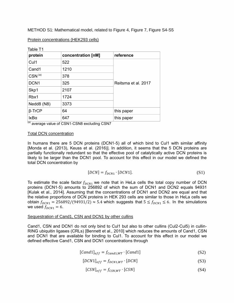
To allow β-TrCP (Fb1) to exhibit a different binding affinity from background SRs we fix 𝑘𝑜𝑛 at the values obtained for Fbxw7 and express the off rate constants for Fb1 and Fb2 in terms of those for Fbxw7 as

𝑘𝑜𝑓𝑓,𝑖𝐹𝑏1 = 𝑓𝐹𝑏1 ∙ 𝑘𝑜𝑓𝑓,𝑖

𝐹𝑏𝑥𝑤7 and 𝑘𝑜𝑓𝑓,𝑖𝐹𝑏2 = 𝑓𝐹𝑏2 ∙ 𝑘𝑜𝑓𝑓,𝑖

𝐹𝑏𝑥𝑤7, 𝑖 = 1,2 (S7)

where 𝑘𝑜𝑓𝑓,1𝐹𝑏𝑥𝑤7 = 9 ∙ 10−7𝑠−1 and 𝑘𝑜𝑓𝑓,2

𝐹𝑏𝑥𝑤7 = 1.3𝑠−1 denote the off rate constants of Skp1•Fbxw7

from the binary and ternary complexes (involving Cand1), respectively [Pierce et al., 2013]. The values of the two scale parameters 𝑓𝐹𝑏1 and 𝑓𝐹𝑏2 were estimated by comparing model predictions with experiments (cf. Parameter estimation and Table T15). Table T3

No. Reactions involving Fb1 𝑘𝑜𝑛 (a)

[(𝑀 ∙ 𝑠)−1]

𝑘𝑜𝑓𝑓

[𝑠−1]

1 Cul1 + Fb1 ↔ Cul1•Fb1

4 ∙ 106 𝑓𝐹𝑏1 ∙ 9 ∙ 10−7

1a Cul1•DCN1 + Fb1 ↔ Cul1•DCN1•Fb1

1b Cul1 + Fb1•S1 ↔ Cul1•Fb1•S1

1c Cul1•DCN1 + Fb1•S1 ↔ Cul1•DCN1•Fb1•S1

1d N8-Cul1 + Fb1 ↔ N8-Cul1•Fb1

1e N8-Cul1 + Fb1•S1 ↔ N8-Cul1•Fb1•S1

1f N8-Cul1•CSN + Fb1 ↔ N8-Cul1•Fb1•CSN

2 Cul1•Cand1 + Fb1 ↔ Cul1•Cand1•Fb1

2 ∙ 106 𝑓𝐹𝑏1 ∙ 1.3 2a Cul1•Cand1•DCN1 + Fb1 ↔ Cul1•Cand1•DCN1•Fb1

2b Cul1•Cand1 + Fb1•S1 ↔ Cul1•Cand1•Fb1•S1

2c Cul1•Cand1•DCN1 + Fb1•S1 ↔ Cul1•Cand1•DCN1•Fb1•S1 (a)

measured for Skp1•Fbxw7 [Pierce et al., 2013]

Table T4

Reactions involving Fb2 𝑘𝑜𝑛

[(𝑀 ∙ 𝑠)−1]

𝑘𝑜𝑓𝑓

[𝑠−1]

Cul1 + Fb2 ↔ Cul1•Fb2

4 ∙ 106 𝑓𝐹𝑏2 ∙ 9 ∙ 10−7

Cul1•DCN1 + Fb2 ↔ Cul1•DCN1•Fb2

Cul1 + Fb2•S2 ↔ Cul1•Fb2•S2

Cul1•DCN1 + Fb2•S2 ↔ Cul1•DCN1•Fb2•S2

N8-Cul1 + Fb2 ↔ N8-Cul1•Fb2

N8-Cul1 + Fb2•S2 ↔ N8-Cul1•Fb2•S2

N8-Cul1•CSN + Fb2 ↔ N8-Cul1•Fb2•CSN

Cul1•Cand1 + Fb2 ↔ Cul1•Cand1•Fb2

2 ∙ 106 𝑓𝐹𝑏2 ∙ 1.3 Cul1•Cand1•DCN1 + Fb2 ↔ Cul1•Cand1•DCN1•Fb2

Cul1•Cand1 + Fb2•S2 ↔ Cul1•Cand1•Fb2•S2

Cul1•Cand1•DCN1 + Fb2•S2 ↔ Cul1•Cand1•DCN1•Fb2•S2

As suggested by our experiments (Fig. 2H) we modeled the assembly of SCF complexes by a random-order binding mechanism (Fig. S4A), i.e. Skp1•F-box receptor proteins may first bind to Cul1 species and then bind substrate or vice versa. In fact, previous simulations indicated that an exchange factor becomes dispensable if binding occurs in a sequential order, i.e. if substrate only binds to F-box proteins if the latter are already bound to Cul1 [Straube et al., 2017]. Cand1 binding to Cul1

The exchange of Skp1•F-box proteins on Cul1 is catalyzed by Cand1 which acts as a substrate receptor exchange factor [Pierce et al., 2013]. Experiments suggest that Cand1 exerts its catalytic function similar to guanine nucleotide exchange factors (GEFs), i.e. through formation of a ternary (Cul1•Cand1•Fb) complex. In the absence of Skp1•F-box proteins spontaneous

dissociation of Cand1 from a Cul1•Cand1 complex is extremely slow (𝑘𝑜𝑓𝑓,3 = 10−5𝑠−1) but

binding of Skp1•F-box to Cul1•Cand1 dramatically increases the dissociation constant for Cand1 in the ternary complex (reaction 4). On thermodynamic grounds (cf. Detailed balance relations) the increase of the dissociation constant for Cand1 upon binding of Skp1•F-box to Cul1•Cand1 must be the same as the increase of the dissociation constant for Skp1•F-box upon binding of Cand1 to Cul1•Skp1•F-box, i.e (cf. Fig. S4C)

𝐾2

𝐾1=

𝐾4

𝐾3= 𝜏 (S8)

where 𝐾𝑖 = 𝑘𝑜𝑓𝑓,𝑖/𝑘𝑜𝑛,𝑖 denotes the dissociation constant of reaction 𝑖. Substituting the known

values for 𝐾1 (0.225𝑝𝑀) and 𝐾2 (650𝑛𝑀) we obtain 𝜏 ≈ 2.9 ∙ 106 which is comparable with values obtained for the GEF-mediated GDP/GTP exchange [Goody & Hofmann-Goody, 2002]. To compute the remaining dissociation constants we measured the rate constants for the association between Cul1 and Cand1 (𝑘𝑜𝑛,3) and that between Cul1•Skp1•Skp2 and Cand1

(𝑘𝑜𝑛,4) (cf. Fig. 1). In this way we obtained 𝐾3 = 0.5𝑝𝑀 and (using Eq. S8) 𝐾4 = (𝐾2/𝐾1)𝐾3 ≈

1.44𝜇𝑀. The latter also determines the dissociation rate constant 𝑘𝑜𝑓𝑓,4 as

𝑘𝑜𝑓𝑓,4 = 𝑘𝑜𝑛,4 ∙ (𝐾2/𝐾1) ∙ 𝐾3 ≈ 2.9𝑠−1.

Reactions 5 and 6 describe the binding of Cand1 to Cul1 when DCN1 is already bound to Cul1. Our pulldown assay with immobilized DCN1 on GST beads showed (Fig. 3C and 3D) that in the

presence of Cand1 the 𝐾𝐷 of DCN1 in the ternary Cul1•Cand1•DCN1 complex is reduced by a

factor 𝛼 = 1/36 = 0.0278 (cf. Fig. S4C). To ensure that the 𝐾𝐷 for Cand1 in the ternary complex

is reduced by the same factor we multiplied the 𝑘𝑜𝑓𝑓 for reaction 5 and 6 by 𝛼 and kept 𝑘𝑜𝑛 the

same as for reactions 3 and 4 (Table T5). Substrate binding to F-box protein

We assumed that substrate binds with equal affinity to free Skp1•F-box proteins as well as to Skp1•F-box proteins that are already bound to Cul1 (Cul1•Fb). In general, our model allows for two substrates that may differ in their binding parameters. In particular simulations S1 represents the phosphorylated form of IκBα (IκBα-P) while S2 plays the role of auxiliary

(background) substrate which is always present in cells. The off rate constant ( 𝑘𝑜𝑓𝑓~10−5𝑠−1)

for the dissociation of IκBα-P from Cul1•β-TrCP•IκBα-P is very small (cf. Fig. S5E) comparable

to that for the dissociation of Skp1•F-box from an SCF complex. The on rate constant has not

been measured, but is expected to lie between 106 − 107(𝑀 ∙ 𝑠)−1. In the simulations we used

the value 𝑘𝑜𝑛 = 107(𝑀 ∙ 𝑠)−1 for both IκBα-P (S1) and auxiliary substrate (S2). Since the latter represents a mixture of different substrates (the type and amount of which is difficult to quantify for our experimental conditions) we assumed a less extreme value for the off rate constant of S2. The reactions involving S1 and S2 are listed in Table T6 and Table T7, respectively. Table T5

No. Reactions 𝑘𝑜𝑛 [(𝑀 ∙ 𝑠)−1] 𝑘𝑜𝑓𝑓 [𝑠−1]

3 Cul1 + Cand1 ↔ Cul1•Cand1 2 ∙ 107 (a) 10−5 (b)

4 Cul1•Fb1 + Cand1 ↔ Cul1•Cand1•Fb1

2 ∙ 106 (a) 2.9 (c) Cul1•Fb2 + Cand1 ↔ Cul1•Cand1•Fb2

4a Cul1•Fb1•S1 + Cand1 ↔ Cul1•Cand1•Fb1•S1

Cul1•Fb2•S2 + Cand1 ↔ Cul1•Cand1•Fb2•S2

5 Cul1•DCN1 + Cand1 ↔ Cul1•Cand1•DCN1 2 ∙ 107 𝛼 ∙ 10−5 (d)

6 Cul1•DCN1•Fb1 + Cand1 ↔ Cul1•Cand1•DCN1•Fb1

2 ∙ 106 𝛼 ∙ 2.9 Cul1•DCN1•Fb2 + Cand1 ↔ Cul1•Cand1•DCN1•Fb2

6a Cul1•DCN1•Fb1•S1 + Cand1 ↔ Cul1•Cand1•DCN1•Fb1•S1

Cul1•DCN1•Fb2•S2 + Cand1 ↔ Cul1•Cand1•DCN1•Fb2•S2 (a)

measured (b)

measured [Pierce et al., 2013], (c)

computed from Eq. (S8), (d)

𝛼 = 0.0278

Table T6

No. Reactions involving S1 𝑘𝑜𝑛 [(𝑀 ∙ 𝑠)−1] 𝑘𝑜𝑓𝑓 [𝑠−1]

7 Fb1 + S1 ↔ Fb1•S1

107 (a) 3.3 ∙ 10−5 (b)

7a Cul1•Fb1 + S1 ↔ Cul1•Fb1•S1

7b Cul1•Cand1•Fb1 + S1 ↔ Cul1•Cand1•Fb1•S1

7c Cul1•DCN1•Fb1 + S1 ↔ Cul1•DCN1•Fb1•S1

7d Cul1•Cand1•DCN1•Fb1 + S1 ↔ Cul1•Cand1•DCN1•Fb1•S1

7e N8-Cul1•Fb1 + S1 ↔ N8-Cul1•Fb1•S1 (a) estimated, (b) measured Table T7

No. Reactions involving S2 𝑘𝑜𝑛 [(𝑀 ∙ 𝑠)−1] 𝑘𝑜𝑓𝑓 [𝑠−1]

Fb2 + S2 ↔ Fb1•S2

107 (a) 0.01 (a)

Cul1•Fb2 + S2 ↔ Cul1•Fb2•S2

Cul1•Cand1•Fb2 + S2 ↔ Cul1•Cand1•Fb2•S2

Cul1•DCN1•Fb2 + S2 ↔ Cul1•DCN1•Fb2•S2

Cul1•Cand1•DCN1•Fb2 + S2 ↔ Cul1•Cand1•DCN1•Fb2•S2

N8-Cul1•Fb2 + S2 ↔ N8-Cul1•Fb2•S2 (a)

estimated

DCN1 binding to Cul1

DCN1 is a scaffold-like E3 ligase which is required for efficient Cul1 neddylation [Kurz et al., 2008]. Experiments have shown that DCN1 forms a stable ternary complex with Cul1 and

Cand1 [Keuss et al., 2016]. In the absence of Cand1 the 𝐾𝐷 for DCN1 binding to Cul1 is comparably low (1.8µ𝑀) [Monda et al., 2013] while binding of Cand1 increases the affinity of

DCN1 to Cul1 36-fold (Fig. 3C and 3D), i.e. the 𝐾𝐷 is lowered by a factor 𝛼 = 1/36 = 0.0278 (cf.

Cand1 binding to Cul1). To generate a 𝐾𝐷 of 1.8µ𝑀 we set 𝑘𝑜𝑛 = 106 (𝑀 ∙ 𝑠)−1 and 𝑘𝑜𝑓𝑓 =

1.8 𝑠−1 (Table T8). When Cand1 is bound to Cul1 we keep 𝑘𝑜𝑛, but lower 𝑘𝑜𝑓𝑓 by a factor 𝛼.

Table T8

No. Reactions 𝑘𝑜𝑛 [(𝑀 ∙ 𝑠)−1] 𝑘𝑜𝑓𝑓 [𝑠−1]

8 Cul1 + DCN1 ↔ Cul1•DCN1

106 (a) 1.8 (b)

8a Cul1•Fb1 + DCN1 ↔ Cul1•DCN1•Fb1

Cul1•Fb2 + DCN1 ↔ Cul1•DCN1•Fb2

8b Cul1•Fb1•S1 + DCN1 ↔ Cul1•DCN1•Fb1•S1

Cul1•Fb2•S2 + DCN1 ↔ Cul1•DCN1•Fb2•S2

9 Cul1•Cand1 + DCN1 ↔ Cul1•Cand1•DCN1

106 α∙ 1.8 (c)

9a Cul1•Cand1•Fb1 + DCN1 ↔ Cul1•Cand1•DCN1•Fb1

Cul1•Cand1•Fb2 + DCN1 ↔ Cul1•Cand1•DCN1•Fb2

9b Cul1•Cand1•Fb1•S1 + DCN1 ↔ Cul1•Cand1•DCN1•Fb1•S1

Cul1•Cand1•Fb2•S2 + DCN1 ↔ Cul1•Cand1•DCN1•Fb2•S2 (a)

estimated, (b)

adjusted so that 𝐾𝐷 = 1.8µ𝑀 [Monda et al., 2013], (c)

α=0.0278

Detailed balance relations

The CRL network contains several thermodynamic cycles two of which are depicted in Fig. S4C. Since each of these cycles comprises only of reversible equilibria there must be no net flux in each cycle at steady state. In physical terms, this means that the change in free energy for the formation of the ternary complexes (Cul1•Cand1•Fb and Cul1•Cand1•DCN1) must not depend on the order in which they are formed. This constraint leads to detailed balance relations

between the dissociation constants in each cycle, i.e. 𝐾1 ∙ 𝐾4 = 𝐾2 ∙ 𝐾3 and 𝐾3 ∙ 𝐾9 = 𝐾5 ∙ 𝐾8. A similar relation also holds for the cycle comprising the reactions 4, 6, 8a, and 9a which leads to

𝐾4 ∙ 𝐾9 = 𝐾8 ∙ 𝐾6. Neddylation reactions

Since DCN1 is required for efficient neddylation of Cul1 [Kurz et al., 2008] and since Cand1 binding and N8 conjugation cannot occur simultaneously [Liu et al., 2002] we assumed that neddylation can only occur from SCF states where DCN1 is bound to Cul1 and Cand1 is not bound to Cul1. In general, Nedd8 (N8) conjugation is catalyzed by an associated E2 enzyme (e.g. UBC12) which is recruited to the Rbx1 domain of an SCF complex. However, the rate constants for E2 binding and N8 conjugation are not known. To keep the number of unknown parameters as small as possible we model neddylation by a first order process (Table T9) with effective neddylation rate constant 𝑘𝑛𝑒𝑑𝑑 which is treated as a variable parameter to be estimated from experiments (cf. Table T15). Also, since the concentration of N8 is much larger

than that of the other proteins (cf. Table T1) we assumed that N8 is not limiting for the reaction so that it can be absorbed into the definition of the rate constant. Table T9

No. Reactions 𝑘𝑛𝑒𝑑𝑑 [𝑠−1]

10 Cul1•DCN1 → N8-Cul1 + DCN1

0.268 (a)

10a Cul1•DCN1•Fb1 → N8-Cul1•Fb1 + DCN1

Cul1•DCN1•Fb2 → N8-Cul1•Fb2 + DCN1

10b Cul1•DCN1•Fb1•S1 → N8-Cul1•Fb1•S1 + DCN1

Cul1•DCN1•Fb2•S2 → N8-Cul1•Fb2•S2 + DCN1 (a)

estimated

Deneddylation reactions

Deneddylation is mediated by the COP9 signalosome (CSN). Consistent with measurements of the rate constants for CSN-mediated deneddylation of N8-Cul1 [Mosadeghi et al., 2016] we assumed that CSN first binds reversibly to N8-Cul1 and N8-Cul1•Fb (11 and 11a) and, in a second step, N8 is cleaved leading to the dissociation of CSN (12 and 12a). Table T10

No. Reactions 𝑘𝑜𝑛 [(𝑀 ∙ 𝑠)−1] 𝑘𝑜𝑓𝑓 [𝑠−1] 𝑘𝑐𝑎𝑡 [𝑠−1]

11 N8-Cul1 + CSN ↔ N8-Cul1•CSN

2 ∙ 107 (a) 0.032 (a) 11a N8-Cul1•Fb1 + CSN ↔ N8-Cul1•Fb1•CSN

N8-Cul1•Fb2 + CSN ↔ N8-Cul1•Fb2•CSN

12 N8-Cul1•CSN → Cul1 + CSN

1.1 (a) 12a N8-Cul1•Fb1•CSN → Cul1•Fb1 + CSN

N8-Cul1•Fb2•CSN → Cul1•Fb2 + CSN (a)

measured [Mosadeghi et al., 2016]

Product inhibition of CSN

While neddylated Cul1 is a substrate of the CSN deneddylated Cul1 acts as an inhibitor of CSN activity [Mosadeghi et al., 2016]. CSN binds to both neddylated and deneddylated Cul1, but with different binding affinity. While the 𝑘𝑜𝑛 is the same for both reactions the 𝑘𝑜𝑓𝑓 for CSN in

complex with non-neddylated Cul1 is increased by a factor of ~200. Previous biochemical analysis has shown that, in the presence of Cand1 or substrate, the deneddylation rate is reduced [Emberley et al., 2012]. Moreover, addition of substrate impedes stable association of CSN with SCF [Enchev et al., 2012]. Hence, to model product inhibition of CSN we assumed that CSN only binds to Cul1, Cul1•Fb, Cul1•DCN1 and Cul1•DCN1•Fb states (cf. Table T11).

Table T11

No. Reactions 𝑘𝑜𝑛 [(𝑀 ∙ 𝑠)−1] 𝑘𝑜𝑓𝑓 [𝑠−1]

13 Cul1 + CSN ↔ Cul1•CSN

2 ∙ 107 (a) 6.2 (a)

13a Cul1•Fb1 + CSN ↔ Cul1•Fb1•CSN

Cul1•Fb2 + CSN ↔ Cul1•Fb2•CSN

13b Cul1•DCN1 + CSN ↔ Cul1•DCN1•CSN

13c Cul1•DCN1•Fb1 + CSN ↔ Cul1•DCN1•Fb1•CSN

Cul1•DCN1•Fb2 + CSN ↔ Cul1•DCN1•Fb2•CSN (a)

measured [Mosadeghi et al., 2016]

Substrate degradation

Substrate degradation by itself is a complex process which involves recruitment of Ub-loaded E2 enzyme to the Rbx1 domain of an SCF complex, subsequent multiple Ub transfers to the substrate and processing by the 26S proteasome. Here, we neglected much of this complexity and assumed that once a substrate-bound SCF complex is neddylated the substrate can be degraded. The latter process was described by first order rate constant 𝑘𝑑𝑒𝑔 which summarizes

the above mentioned processes in an effective manner (Table T12). Also, for simplicity we assumed that the degradation rate constant is the same for S1 (IκBα-P) and background substrate S2. For the human 26S proteasome substrate degradation rates range from less than

0.01 𝑚𝑖𝑛−1 up to 0.7 𝑚𝑖𝑛−1 depending on the substrate and the number of conjugated ubiquitins

[Lu et al., 2016]. For CyclinB-NT with 4 conjugated ubiquitins the degradation rate is 0.5 𝑚𝑖𝑛−1

or 0.0083 𝑠−1. Based on our measurements we estimated 𝑘𝑑𝑒𝑔 = 0.0071 𝑠−1 (cf. Table T15).

Table T12

No. Reactions 𝑘𝑑𝑒𝑔 [𝑠−1]

14 N8-Cul1•Fb1•S1 → N8-Cul1•Fb1 0.0071

(a)

N8-Cul1•Fb2•S2 → N8-Cul1•Fb2 (a)

estimated

Background substrate

To generate the high degree of Cul1 neddylation observed experimentally we had to assume that cells contain a certain amount of CRL substrates, which is consistent with the fact that substrate favors the neddylated state of CRL ligases [Emberley et al., 2012; Enchev et al., 2012]. To generate auxiliary substrate we assumed a constitutive synthesis term (Table T13). Since the total amount of background CRL substrates in the cell is unknown we treated the synthesis rate as a variable parameter to be determined by comparison with experiments (cf. Table T15). In this way we obtained an estimate of 2261nM for the concentration of background substrate under steady state conditions in wildtype cells assuming that substrates are only degraded via the CRL-mediated pathway. Table T13

No. reaction 𝑘𝑠𝑦𝑛𝑡ℎ𝑆2 [𝑛𝑀 ∙ 𝑠−1]

15 Ø → S2 1.4 (a)

(a) estimated

Simulations were done with the Systems Biology Toolbox of MATLAB [MATLAB 2015b] which was used to translate the model reactions (1-15) into a system of ordinary differential equations using mass-action kinetics. Integrations were performed with the implicit solver ode15s. Parameter estimation

To validate our model we measured different quantities in wildtype (WT) cells as well as in response to different genetic perturbations (cf. Table T14). Conditions listed in bold font were used to estimate the values of unknown parameters. Altogether, our model comprises 54 state variables and 35 parameters (rate constants, protein concentrations and scale parameters) from which 22 parameters were either known from previous experiments or measured in this work. Among the 13 remaining parameters 8 parameters could be reasonably estimated or constrained leaving only 5 parameters to be fitted by comparing model simulations with experiments. The 4 scale factors P1 – P4 (Table T15) were estimated based on relative protein abundances and previous measurements of the association of Cand1 with different cullins. The 4 on and off rate constants P5 – P8 had almost no effect on the value of the measured quantities (cf. T14 and Fig. S5B), so we fixed them at the indicated values to reduce the number of variable parameters during the fitting procedure. Table T14 – Experimental conditions and measured quantities

measured quantity cell type / perturbation / condition type of experiment figure

Cul1.b2.Cand1(a)

WT(e)

/ WT + MLN4924 steady state 4B

Cul1.b2.Skp1(b) WT / WT + MLN4924 / DKO

(f) steady state 4B

Cul1.b2.N8(c) WT / WT + Cul1 / DKO / DKO + Cul1 steady state 4E

β-TrCP.b2.Cul1(d)

WT steady state 4D

𝑡1/2 WT / DKO / DKO + Cand1

transient

4C

WT + β-TrCP / WT + Cul1 / DKO + β-TrCP / DKO + Cul1

4F

(a) fraction of Cul1 bound to Cand1,

(b) fraction of Cul1 bound to Skp1,

(c) fraction of Cul1 bound to Nedd8,

(d) fraction of β-TrCP bound to Cul1,

(e) WT – wildtype,

(f) DKO – double knockout Cand1

-/-, Cand2

-/-

To estimate the values of the 5 remaining parameters in Table T15 (P9-P13) we used nonlinear optimization in combination with a profile likelihood approach as described in [Raue et al., 2009]. To calibrate the model we defined the weighted sum of squared residuals as an objective function

𝜒2(𝜃) ≔ ∑

(𝑦𝑘 − 𝑦𝑘(𝜃))2

𝜎𝑘2

6

𝑘=1

(S9)

and numerically determined 𝜃 = (𝑓𝐹𝑏1

, 𝑓𝐹𝑏2

, 𝑘𝑛𝑒𝑑𝑑, 𝑘𝑑𝑒𝑔, 𝑘𝑠𝑦𝑛𝑡ℎ𝑆2 ) such that

𝜃 = argmin [𝜒2(𝜃)].

In Eq. (S9) 𝑦𝑘 and 𝜎𝑘2 denote the values of the measured quantities (cf. T14, bold face) and

their respective measurement errors. The quantities 𝑦𝑘(𝜃) are the predicted values of the measured quantities obtained from numerical simulations of our model for a particular set of parameter values. Due to limited sample size we were not able to reliably estimate the measurement errors from the data. So, for convenience, we assumed equal variances of

𝜎𝑘2 = 0.1𝑦𝑘 (10% from the mean values) for all measurements. However, since all parameters

are identifiable (see below) a different choice for the values of the variances would yield qualitatively similar results. To obtain confidence intervals for the estimated parameter values we numerically computed the profile likelihood for each parameter defined as

𝜒𝑃𝐿

2 (𝜃𝑖) = min𝜃𝑗≠𝑖[𝜒2(𝜃)], (S10)

i.e. for each value of 𝜃𝑖 the objective function defined in Eq. (S9) was re-optimized with respect to the remaining parameters 𝜃𝑗≠𝑖 . The resulting plots exhibit a parabolic shape (Fig. S5A)

indicating that all parameters are identifiable [Raue et al., 2009]. To obtain finite sample confidence intervals we defined the confidence regions

{𝜃𝑖: 𝜒𝑃𝐿

2 (𝜃) − 𝜒2(𝜃) < 𝛥𝛼}, 𝑖 = 1, … ,5 (S11)

where the threshold 𝛥𝛼 = 𝜒2(𝛼, 𝑑𝑓) is the 𝛼 quantile (confidence level) of the 𝜒2-distribution with 𝑑𝑓 degrees of freedom. Pointwise confidence intervals are obtained for 𝑑𝑓 = 1 while 𝑑𝑓 = 5 yields simultaneous confidence intervals for all 5 parameters. Confidence intervals for model predictions (cf. Fig. 4) were computed by running simulations for parameters sampled from the

confidence region defined by Eq. (S11) with the threshold 𝛥𝛼 = 𝜒2(0.95,5) (Fig. S5A, upper horizontal line). Table T15 – List of estimated parameters

parameter value expected range defined in fixed / variable

P1 𝑓𝐷𝐶𝑁1 6 5 − 6 Eq. (S1) fixed

P2 P3

𝑓𝐷𝐶𝑁1,𝑊𝑇

𝑓𝐶𝑆𝑁,𝑊𝑇 0.23

Eqs. (S2) – (S4) fixed

P4 𝑓𝐶𝑎𝑛𝑑1,𝑊𝑇 0.54 fixed

P5 𝑘𝑜𝑛𝑆1 107 (𝑀𝑠)−1 106 − 107 (𝑀𝑠)−1 Table T6 fixed

P6 𝑘𝑜𝑛𝑆2 107 (𝑀𝑠)−1 106 − 107 (𝑀𝑠)−1 Table T7 fixed

P7 𝑘𝑜𝑓𝑓𝑆2 0.01𝑠−1 0.0001 − 0.01 𝑠−1 Table T7 fixed

P8 𝑘𝑜𝑛𝐷𝐶𝑁1 106 (𝑀𝑠)−1 106 − 107 (𝑀𝑠)−1 Table T8 fixed

P9 𝑓𝐹𝑏1 0.247 0.102 − 0.490 (a)

Eq. (S7) variable

P10 𝑓𝐹𝑏2 6.514 2.978 − 17.461 (a)

Eq. (S7) variable

P11 𝑘𝑛𝑒𝑑𝑑 0.268 𝑠−1 0.134 − 0.626 𝑠−1 (a)

Table T9 variable

P12 𝑘𝑑𝑒𝑔 0.0071 𝑠−1 0.0055 − 0.0091 𝑠−1 (a)

Table T12 variable

P13 𝑘𝑠𝑦𝑛𝑡ℎ𝑆2 1.40 𝑛𝑀 ∙ 𝑠−1 1.09 − 1.85 𝑛𝑀 ∙ 𝑠−1

(a) Table T13 variable

(a) simultaneous confidence intervals to a 95% confidence level with 10% assumed measurement errors.

Response coefficients

To quantify how small changes in one of the parameters (P5 – P13) would impact the predicted values for the measured quantities (cf. T14) we computed the matrix of response coefficients (Fig. S5B) according to

𝑅𝑖𝑗 ≔

∆𝑄𝑖/𝑄𝑖𝑟𝑒𝑓

∆𝑃𝑗/𝑃𝑗𝑟𝑒𝑓

(S12)

where ∆𝑃𝑗 = 𝑃𝑗 − 𝑃𝑗𝑟𝑒𝑓

denotes the change of parameter 𝑃𝑗 relative to a reference value 𝑃𝑗𝑟𝑒𝑓

and ∆𝑄𝑖 = 𝑄𝑖 − 𝑄𝑖𝑟𝑒𝑓

represents the corresponding change of the predicted quantity 𝑄𝑖 .

Depending on whether 𝑄𝑖 increases or decreases upon a parameter change ∆𝑃𝑗 the response

coefficient 𝑅𝑖𝑗 may be positive or negative, respectively. Its magnitude quantifies the fractional

change of 𝑄𝑖 upon a fractional change of 𝑃𝑗. The fact that almost all response coefficients satisfy

|𝑅𝑖𝑗| < 1 means that our system exhibits only a weak sensitivity to most of the parameters at the

respective reference point. This is particularly true for the 4 on and off rate constants P5 – P8

which have almost no effect on the predicted values of the measured quantities except for 𝑘𝑜𝑛𝐷𝐶𝑁

which weakly affects the half-life for substrate degradation in DKO cells. To reduce the number of fitting parameters we have, therefore, fixed P5 – P8 during parameter estimation. From the entries of the response matrix for the remaining parameters (P9 – P13) we can make some interesting observations: The fractions of Cul1 bound to Cand1, Skp1 and Nedd8 (first

three rows) are mainly determined by the ratio between substrate synthesis ( 𝑘𝑠𝑦𝑛𝑡ℎ𝑆2 ) and

degradation (𝑘𝑑𝑒𝑔). If the substrate synthesis rate is increased the neddylated fraction of Cul1

increases and more Skp1•F-box proteins are recruited to Cul1 leading to a reduction of the fraction of Cul1 associated with Cand1. Increasing 𝑘𝑑𝑒𝑔 has the opposite effect. However, the

latter also affects the half-life for IκBα degradation while 𝑘𝑠𝑦𝑛𝑡ℎ𝑆2 has only a minor effect on 𝑡1/2.

Interestingly the total concentration of Skp1•F-box proteins (FbT) has a strong positive effect on the half-life for IκBα degradation in DKO cells because increasing the total pool of F-box proteins reduces the amount of Cul1 available for binding to β-TrCP. Protein fractions in terms of state variables

To relate the measured quantities defined in Table T14 to state variables in our model (cf. Table 2) we used the following relations: The fraction of Cul1 bound to Nedd8 was computed as

Cul1. b2. N8 =[N8˗Cul1] + [N8˗Cul1 • Fb1] + [N8˗Cul1 • Fb2]

Cul1T

+[N8˗Cul1 • Fb1 • S1] + [N8˗Cul1 • Fb2 • S2] + [N8˗Cul1 • CSN]

Cul1T

+[N8˗Cul1 • Fb1 • CSN] + [N8˗Cul1 • Fb2 • CSN]

Cul1T

where 𝐶𝑢𝑙1𝑇 denotes the total concentration of Cul1 defined in Table T1. To define the fractions of Cul1 bound to Cand1 (Cul1.b2.Cand1) and Cul1 bound to Skp1•F-box (Cul1.b2.Skp1) we had to take into account that higher-order complexes involving Cand1 and Fb1 or Fb2 are unstable and, thus, cannot be detected in our pull-down assays. For example, the complexes Cul1•Cand1•Fbi•Si would rapidly decay into Cul1•Fbi•Si and Cand1 or Cul1•Cand1 and Fbi•Si (Fig. S5C). The corresponding probabilities are given by

𝑎𝑖 =𝑘𝑜𝑓𝑓,2

𝑆𝑖

𝑘𝑜𝑓𝑓,2𝑆𝑖 + 𝑘𝑜𝑓𝑓,4

and 𝑏𝑖 = 1 − 𝑎𝑖 =𝑘𝑜𝑓𝑓,4

𝑘𝑜𝑓𝑓,2𝑆𝑖 + 𝑘𝑜𝑓𝑓,4

, 𝑖 = 1,2 (S13)

where the rate constants 𝑘𝑜𝑓𝑓,2𝑆𝑖 and 𝑘𝑜𝑓𝑓,4 are defined in Tables T3-T5. For the decay of

complexes involving Cand1, DCN1 and Fb1 or Fb2 we considered three decay channels as the dissociation of Cand1 and DCN1 from Cul1•Cand1•DCN1•Fbi•Si or Cul1•Cand1•DCN1•Fbi occurs with similar rates. The respective probabilities are given by

𝑐𝑖 =𝑘𝑜𝑓𝑓,2

𝑆𝑖

𝑘𝑜𝑓𝑓,2𝑆𝑖 + 𝑘𝑜𝑓𝑓,6 + 𝑘𝑜𝑓𝑓,9

, 𝑑𝑖 =𝑘𝑜𝑓𝑓,6

𝑘𝑜𝑓𝑓,2𝑆𝑖 + 𝑘𝑜𝑓𝑓,6 + 𝑘𝑜𝑓𝑓,9

, 𝑒𝑖 = 1 − (𝑐𝑖 + 𝑑𝑖), (S14)

for 𝑖 = 1,2 where the rate constants 𝑘𝑜𝑓𝑓,6 and 𝑘𝑜𝑓𝑓,9 are defined in Tables T5 and T8,

respectively. With the help of these probabilities the protein fractions Cul1.b2.Cand1 and Cul1.b2.Skp1 (which we set equal to Cul1.b2.Fb1+Cul1.b2.Fb2) are defined by

Cul1. b2. Cand1 =[Cul1 • Cand1] + 𝑎1([Cul1 • Cand1 • Fb1] + [Cul1 • Cand1 • Fb1 • S1])

Cul1T

+𝑎2([Cul1 • Cand1 • Fb2] + [Cul1 • Cand1 • Fb2 • S2]) + [Cul1 • Cand1 • DCN1]

Cul1T

+(𝑎1𝑒1 + 𝑐1)([Cul1 • Cand1 • DCN1 • Fb1] + [Cul1 • Cand1 • DCN1 • Fb1 • S1])

Cul1T

+(𝑎2𝑒2 + 𝑐2)([Cul1 • Cand1 • DCN1 • Fb2] + [Cul1 • Cand1 • DCN1 • Fb2 • S2])

Cul1T

and

Cul1. b2. Fbi =[Cul1 • Fbi] + [Cul1 • Fbi • Si] + [Cul1 • DCN1 • Fbi]

Cul1T

+𝑏𝑖([Cul1 • Cand1 • Fbi] + [Cul1 • Cand1 • Fbi • Si])

Cul1T

+(𝑏𝑖𝑒𝑖 + 𝑑𝑖)([Cul1 • Cand1 • DCN1 • Fbi] + [Cul1 • Cand1 • DCN1 • Fbi • Si])

Cul1T

+[N8˗Cul1 • Fbi] + [N8˗Cul1 • Fbi • Si] + [N8˗Cul1 • Fbi • CSN]

Cul1T

+[Cul1 • DCN1 • Fbi • CSN] + [Cul1 • Fbi • CSN] + [Cul1 • DCN1 • Fbi • Si]

Cul1T

for 𝑖 = 1,2. The fraction of β-TrCP bound to Cul1 (β-TrCP.b2.Cul1) is given by

β˗TrCP. b2. Cul1 = Cul1. b2. Fb1Cul1T

Fb1T

where Fb1T equals the total β-TrCP concentration listed in Table T1. Simulation protocols

To simulate IκBα degradation of we started simulations from steady state by adding the reaction

No. reaction 𝑘𝑝ℎ𝑜𝑠 [𝑠−1] initial condition

16 IκBα → IκBα-P (S1) ln(2) /(60 ∙ 14) [IκBα]=647nM

which describes the phosphorylation of IκBα by IκBα kinase. Phosphorylated IκBα (IκBα-P) is

generated with a half-life of 14min serving as a substrate of the SCFβ-TrCP ligase (Cul1 • Fb1). To simulate the conditions and perturbations listed in Table T14 we used the protocols defined in Table T16. Inhibition of Nedd8 conjugation as well as Cand1-/-, Cand2-/- double knockout were simulated by setting the neddylation rate constant and the total Cand1 concentration to zero, respectively. To simulate Cul1 overexpression we computed a scale factor assuming that Cul1 competes with other cullins for access to Rbx1. Similarly, to simulate β-TrCP overexpression we computed a scale factor assuming that β-TrCP competes with auxiliary SRs for access to Skp1. In the case of Cul1 overexpression we also had to recompute the scale factors that account for sequestration of DCN1, CSN and Cand1 by other cullins. In both cases the overexpression factors (𝑓𝐶𝑢𝑙1 and 𝑓β˗TrCP) account for both endogenous and exogenous proteins.

Table T16

perturbation protocol remark

WT + MLN4924 set 𝑘𝑛𝑒𝑑𝑑 = 0 at 𝑡 = 0 Inhibition of Nedd8 conjugation

DKO set [𝐶𝑎𝑛𝑑1] = 0 at 𝑡 = 0 Cand1

-/-, Cand2

-/-

double knockout

WT / DKO + Cul1

set [𝐶𝑢𝑙1]𝑂𝐸 = 𝑓𝑂𝐸,𝐶𝑢𝑙1 ∙ [𝐶𝑢𝑙1]𝑊𝑇(𝑎)

with

𝑓𝑂𝐸,𝐶𝑢𝑙1(𝑏) =

𝑓𝐶𝑢𝑙1[𝑅𝑏𝑥1]

[𝑅𝑏𝑥1] + (𝑓𝐶𝑢𝑙1 − 1)[𝐶𝑢𝑙1]𝑊𝑇

and recompute scale factors in Eqs. (S2) – (S4)

𝑓𝐷𝐶𝑁1,𝑂𝐸(𝑐) =

[𝐶𝑢𝑙1]𝑂𝐸

[𝐶𝑢𝑙1]𝑂𝐸 + [𝑅𝑏𝑥1] − [𝐶𝑢𝑙1]𝑊𝑇 + [𝐶𝑢𝑙5]

𝑓𝐶𝑎𝑛𝑑1,𝑂𝐸(𝑑) = 𝑚𝑖𝑛 (1, 𝑓𝐶𝑎𝑛𝑑1,𝑊𝑇

𝑓𝐷𝐶𝑁1,𝑂𝐸

𝑓𝐷𝐶𝑁1,𝑊𝑇

)

Cul1 overexpres-sion in WT or DKO

WT / DKO + β-TrCP

set [𝐹𝑏1]𝑂𝐸 = 𝑓𝑂𝐸,β˗TrCP ∙ [𝐹𝑏1]𝑊𝑇(𝑒)

with

𝑓𝑂𝐸,β˗TrCP(𝑓) =

𝑓β˗TrCP[𝐹𝑏𝑇]𝑊𝑇

[𝐹𝑏𝑇]𝑊𝑇 + (𝑓β˗TrCP − 1)[𝐹𝑏1]𝑊𝑇

set [𝐹𝑏𝑇]𝑂𝐸 = [𝐹𝑏𝑇]𝑊𝑇 − [𝐹𝑏1]𝑂𝐸

β-TrCP overex-pression in WT or DKO

(a) [𝐶𝑢𝑙1]𝑊𝑇 = 522𝑛𝑀,

(b) 𝑓𝐶𝑢𝑙1 = 6.6 in WT and 𝑓𝐶𝑢𝑙1 = 5 in DKO,

(c) 𝑓𝐶𝑆𝑁,𝑂𝐸 = 𝑓𝐷𝐶𝑁1,𝑂𝐸 ,

(d) not applicable in

DKO, (e)

[𝐹𝑏1]𝑊𝑇 = 64𝑛𝑀, (f)

𝑓β˗TrCP = 5.5 in WT and 𝑓β˗TrCP = 8 in DKO, [𝐹𝑏𝑇]𝑊𝑇 = 2107𝑛𝑀

Computation of the cycle time

To compute the cycle time for the cyclic reaction chain depicted in Fig. 7 we assigned to each reversible reaction an effective forward rate constant using the concept of net rate constants

[Cleland, 1975]. The latter are denoted by 𝑘1,…,𝑘6 in Fig. S5D (highlighted in red color). For irreversible reactions such as neddylation (𝑘10) and deneddylation (𝑘12) the net rate constant is identical with the rate constant. Then the net rate constant 𝑘6 is given by

𝑘6 = 𝑘𝑜𝑛,11[𝐶𝑆𝑁]𝑘12

𝑘12 + 𝑘𝑜𝑓𝑓,11 (S15)

where [𝐶𝑆𝑁] = 82𝑛𝑀 denotes the concentration of free (unbound) CSN under steady state conditions (with [S1]=0). The other 5 net rate constants are defined recursively as

𝑘5 = 𝑘𝑜𝑓𝑓,6

𝑘10

𝑘10 + 𝑘𝑜𝑛,6[𝐶𝑎𝑛𝑑1] (S16)

𝑘4 = 𝑘𝑜𝑛,2([𝐹𝑏1] + [𝐹𝑏2] + [𝐹𝑏2 • 𝑆2])𝑘5

𝑘5 + 𝑘𝑜𝑓𝑓,2 (S17)

𝑘3 = 𝑘𝑜𝑛,9[𝐷𝐶𝑁1]𝑘4

𝑘4 + 𝑘𝑜𝑓𝑓,9 (S18)

𝑘2 = 𝑘𝑜𝑓𝑓,2

𝑘3

𝑘3 + 𝑘𝑜𝑛,2[𝐹𝑏1] (S19)

𝑘1 = 𝑘𝑜𝑛,4[𝐶𝑎𝑛𝑑1]𝑘2

𝑘2 + 𝑘𝑜𝑓𝑓,4. (S20)

The concentrations for Cand1, Fb1 (β-TrCP), Fb2 (auxiliary SR), Fb2•S2 and DCN1 are steady state concentrations that were obtained by integrating the model equations using the parameter set for WT cells (Tables T2-T13, T15) without substrate for Fb1. Note that in Eq. (S14) the factor in front of the fraction represents the effective “on rate” for binding of any free Skp1•F-box protein to Cul1•Cand1•DCN1 while in Eq. (S16) we used the on rate for binding of a particular F-box protein (Fb1) to bind to Cul1•Cand1. Combining the expressions in Eq. (S15) – (S20) yields the estimate for the average cycle time

𝑡𝑐𝑦𝑐𝑙𝑒 =1

𝑘1+

1

𝑘2+

1

𝑘3+

1

𝑘4+

1

𝑘5+

1

𝑘6+

1

𝑘10+

1

𝑘12. (S21)

Supplemental References

Cleland, W.W. (1975). Partition analysis and the concept of net rate constants as tools in enzyme kinetics. Biochemistry 14, 3220–3224. Emberley, E.D., Mosadeghi, R., and Deshaies, R.J. (2012). Deconjugation of Nedd8 from Cul1 is directly regulated by Skp1-F-box and substrate, and the COP9 signalosome inhibits deneddylated SCF by a noncatalytic mechanism. J. Biol. Chem. 287, 29679–29689. Enchev, R.I., Scott, D.C., da Fonseca, P.C., Schreiber, A., Monda, J.K., Schulman, B.A., Peter, M., and Morris, E.P. (2012). Structural basis for a reciprocal regulation between SCF and CSN. Cell Rep. 2, 616–627. Keuss, M.J., Thomas, Y., Mcarthur, R., Wood, N.T., Knebel, A., and Kurz, T. (2016). Characterization of the mammalian family of DCN-type NEDD8 E3 ligases. J. Cell Sci. 129, 1441–1454.

Kulak, N.A., Pichler, G., Paron, I., Nagaraj, N., and Mann, M. (2014). Minimal, encapsulated proteomic-sample processing applied to copy-number estimation in eukaryotic cells. Nat. Methods 11, 319–324. Kurz, T., Chou, Y.C., Willems, A.R., Meyer-Schaller, N., Hecht, M.L., Tyers, M., Peter, M., and Sicheri, F. (2008). Dcn1 functions as a scaffold-type E3 ligase for cullin neddylation. Mol. Cell 29, 23–35. Liu, J., Furukawa, M., Matsumoto, T., and Xiong, Y. (2002). NEDD8 modification of CUL1 dissociates p120(CAND1), an inhibitor of CUL1-SKP1 binding and SCF ligases. Mol. Cell 10, 1511–1518. Lu, Y., Lee, B.H., King, R.W., Finley, D., and Kirschner, M.W. (2015). Substrate degradation by the proteasome: a single-molecule kinetic analysis. Science 348, 1250834. Raue, A., Kreutz, C., Maiwald, T., Bachmann, J., Schilling, M., Klingmüller, U., and Timmer, J. (2009). Structural and practical identifiability analysis of partially observed dynamical models by exploiting the profile likelihood. Bioinformatics 25, 1923–1929. Schulman, B.A., Carrano, A.C., Jeffrey, P.D., Bowen, Z., Kinnucan, E.R.E., Finnin, M.S., Elledge, S.J., Harper, J.W., Pagano, M., and Pavletich, N.P. (2000). Insights into SCF ubiquitin ligases from the structure of the Skp1-Skp2 complex. Nature 408, 381–386.