1

Instructions for authors "Coastal Ecosystems" is an open-access online journal

aiming at the dissemination of scientific results and ideas

in the field of coastal ecosystems studies. It accepts

submissions from all interested individuals irrespective of

SCESAP membership.

Manuscript submission

Submission of a manuscript implies: that the work described has not been published before; that it is not under

consideration for publication anywhere else; that its

publication has been approved by all co-authors, if any, as

well as by the responsible authorities – tacitly or explicitly

– at the institute where the work has been undertaken.

Any submission which violates these will be rejected, with

the author names possibly placed on our blacklist and the

information being shared with other journals. Neither the

SCESAP nor its Editorial Office will be held legally

responsible should there be any claims for compensation.

Manuscript prepared in accordance with the following

instructions should be submitted to the Journal editorial office via e-mail [ journal(at)scesap.org ] or using its online

submission system. In case e-mail/online submission is not

possible, a CD/DVD/USB stick may be submitted by

ordinary postal service to:

Coastal Ecosystems Editorial Office AMBL - Kyushu University Reihoku-Amakusa, Kumamoto 863-2507, Japan TEL: +81-969-35-0003 FAX: +81-969-35-2413

Submitted manuscripts will first be checked for language,

presentation, and style. Authors for whom English is a

second language are strongly advised to have their

manuscripts professionally checked before submission.

Manuscripts which are substandard in these respects

(including formatting as described in this document)

will be returned without review. Papers which conform

to journal scope, aims and style are sent to at least 2

referees. Manuscripts returned to authors with referee

reports should be revised and sent back to the editorial office as soon as possible. Final decisions on acceptance or

rejection are made by the Editor-In-Chief.

Publication fees

There is no publication charge for submitted papers if the

first author is a registered SCESAP member. Non-member

first author papers will incur publication fees as designated

on the journal web site.

1. Manuscript types

There are four categories of papers:

(1) Regular papers; (2) Review papers; (3) Forum

papers; (4) Data papers.

All papers must have an Abstract (see below). “Regular

papers” are research papers consisting of Abstract,

Introduction, Materials and Methods, Results, and

Discussion. “Review papers” can deal with any topic of

interest to the journal, including management and

conservation issues relating to coastal ecosystems. “Forum

papers” concern a discussion of a particular topic, e.g. methodology, equipment, statistics, conceptual issues, etc.

A single topic concerning the management and

conservation of coastal ecosystems and their biological

components can also be dealt with as a Forum paper.

Forum papers do not have separate Introduction, Materials

and methods, Results, and Discussion, but the authors can

use subsections where necessary. “Data papers” are

mainly concerned with presenting fairly extensive data sets

of scientific interest (including checklists of species),

which may be used/referenced by wider scientific

community, consisting of Introduction, Materials and

methods, and Data explanation (a section corresponding to ‘Results’ in ordinary papers). Any data,

biological/physical/chemical, can be presented, but their

biological implications need to be clearly but concisely

explained, with a minimum of speculative interpretations.

2

The editors reserve the right to decide on the categorisation

of a submitted/accepted paper.

2. Formatting

à STUDY CAREFULLY THE MODEL MS ATTACHED AT

THE END OF THIS DOCUMENT or on the website

(1) Manuscripts for reviewing should be submitted as a

single PDF file in a zip folder with your name, e.g.

charlesdarwin.zip. To do this, place your file(s) in a folder

entitled with your name and then compress it with zip. Upon acceptance, the final manuscripts must be submitted

in MS Word (docx, doc) or RTF format for text and tables,

and EPS, JPEG, TIFF, AI (Illustrator - preferred) or PSD

(Phtoshop – preferred) for figures (see below for

instructions on figure preparation).

(2) Preferably, 12-point Arial or Times Roman font should

be used, with 1.5 line spacing and 25mm margins for top

and bottom and 20-23mm left and right.

(3) Do NOT align the text on both sides; align to the left

only, as in this instruction document.

(4) Pages and lines must be numbered (in particular,

consecutive line numbers throughout the text). (5) Use italics for emphasis, genus and species name.

(6) Use tab stops or other commands for indents, not the

space bar.

(7) Use the table function, not spreadsheets, to make tables.

(8) Use the equation editor for equations.

(9) Please use no more than three levels of displayed

headings.

(10) Abbreviations should be defined at first mention and

used consistently thereafter.

Units, symbols and abbreviations

Follow the International System of Units (SI, Système International d'Unités) where possible for all measurements.

Mathematical expressions should contain symbols, not

abbreviations. If the paper contains many symbols, define

them as early in the text as possible, or within a subsection

of the Materials and methods section.

Scientific names

Give the Latin name of each species in full, together with

the authority for its name, at first mention in the main text

or in a Table. If they appear in the Summary/Abstract, use

the common and Latin name only in the first instance, then

the Latin or common name thereafter. If there are many species, provide a table or cite a checklist which may be

consulted for authorities instead of listing them in the text.

Do not give authorities for species cited from published

references. Give priority to scientific names in the text

(with colloquial names in parentheses, if desired).

Equipment's names

Clarify the manufacturer’s names of major equipment used

in the work, where applicable.

Mathematical expressions

Mathematical expressions should be carefully represented. Avoid confusions between similar characters, e.g. 'l' (el)

and '1' (one). Also make sure that expressions are spaced as

you would like them to appear, and if there are several

equations, they should be identified by eqn 1, etc.

Numbers in text and tables

Avoid using an unnecessary number of digits when writing

a decimal number; the number of digits should reflect the

precision of the measurement.

3. Manuscript components

Manuscripts should conform to standard rules of English

grammar and style. Either British or American spelling

may be used, but consistently throughout the article.

Editors reserve the right to modify manuscripts that do not

conform to scientific, technical, stylistic or grammatical

standards.

(a) Title page should contain:

(a-1) Title.

(a-2) A list of authors' names with their affiliations

and addresses. (a-3) A running headline (< 50 characters).

(a-4) The name, e-mail address, telephone and fax

numbers of the corresponding author.

3

(b) Abstract should summarise the main results and

conclusions of the paper in (up to) 250 words. The abstract

should not contain any undefined abbreviations or

unspecified references. Avoid including numerical results, as details are more often than not distracting than being

essential/helpful in the abstract.

(b-1) Keywords. Provide 4 to 6 keywords on the

abstract page, listed in alphabetical order. Avoid

choosing as keywords those that are already in the

title or abstract, such that potential readers from

wider areas who might not otherwise pick up your

paper are drawn in when using search engines.

(c) Introduction

This should state the background of the work, the nature of

the hypothesis or hypotheses under consideration (if any), and should outline the essential background.

(d) Materials and Methods

This should provide sufficient details of the techniques to

enable the work to be repeated.

(e) Results

This should state the results, drawing attention in the text

to important details shown in tables and figures.

(f) Discussion

This should point out the significance of the results in relation to the reasons for doing the work, and place them

in the context of other works. Discussion should not be

combined with Results.

(g) Acknowledgments

Acknowledgments of people, grants, funds, etc. should be

placed in a separate section before the reference list. The

names of funding organizations should be written in full.

(h) References

References in the text to works by up to three authors

should be in full, e.g. (Arakaki & Tokeshi 2011; Yeemin, Sutthacheep & Pettongma 2006). If there are more than

three authors, they should always be abbreviated thus:

(Susanto et al. 2013). When different groups of authors

with the same first author and date occur, they should be

cited thus: (Darwin, Yucharoen & Samsuvan 1850a;

Darwin, Sangmanee & Wongthepwanit 1850b), then

subsequently abbreviated to (Darwin et al. 1850a, b). The

references in the list should be in alphabetical order with the journal name in full. Use the indent function of MS

WORD to indent the second and subsequent lines of each

entry; do NOT use the space bar to indent - if unsure, do

not indent at all. The format for papers, entire books,

chapters in books, and PhD theses is as follows.

Fortes MD (1988) Indo-West Pacific affinities of

Philippine Seagrasses. Botanica Marina 31, 237-242.

Gomez ED, Aliño PM, Licuanan WRY & Yap HT (1994)

Status report on coral reefs of the Philippines 1994. In:

CR Wilkinson, S Sudara & LM Chou (eds.), pp. 57-76.

(Vol 1) Proc. 3rd ASEAN-Australia Symposium on Living Coastal Resources, Chulalongkorn University,

Bangkok.

Kawai T & Tokeshi M (2007) Testing the

facilitation-competition paradigm under the

stress-gradient hypothesis: decoupling multiple stress

factors. Proceedings of the Royal Society, London, B

274, 2503-2508.

Ota N (2001) Resource utilisation and coexistence in

congeneric predatory-scavenging snails, Japeuthria

ferrea and J. cingulata. PhD thesis, Kyushu University,

Fukuoka.

Titlyanov EA, Titlyanova TV & Chapman DJ (2008) Dynamics and patterns of algal colonization on

mechanically damaged and dead colonies of the coral

Porites lutea. Botanica Marina 51, 285- 296.

Tokeshi M (1999) Species Coexistence: Ecological and

Evolutionary Perspectives. Blackwell Science, Oxford.

Yap HT, Alino PM & Gomez ED (1992) Trends in growth

and mortality of three coral species (Anthozoa:

Scleractinia), including effects of transplantation.

Marine Ecology Progress Series 83, 91-101.

References should only be cited as 'in press' if the paper

has been accepted for publication. Citations from the world-wide-web are only allowed when alternative hard

literature sources do not exist for the cited information.

Fully authenticated addresses are included in the reference

list, along with titles, years and authors of the sources

4

being cited. The sites or information sources have

sufficient longevity and ease of access for others to follow

up the citation. The information is of a scientific quality at

least equal to that of peer reviewed information available in learned scientific journals.

(i) Tables

All tables are to be numbered using Arabic numerals.

Tables should always be cited in text in consecutive

numerical order. Each table should be on a separate page,

numbered, with a table caption explaining the table

components at the top. Each table must be understandable

on its own, i.e. without referring to the main text. Units

must be clearly indicated. Include references at the end of

the table caption, if any previously published material is

included in the table. Footnotes to tables should be indicated by superscript lower-case letters (or asterisks for

significance values and other statistical data) and included

beneath the table body. Do not present the same data in

both figure and table forms.

(j) Figures

All figures must be prepared in an electronic format: AI

(Illustrator - preferred for graphs), PSD, EPS, JPEG

(preferred for photos), TIFF or MS office files (but note

that EXCEL graphs are often not good enough). Figures

should not be embedded into the main text and each should

be on a separate page. For reviewing, all figures should be converted to PDF and attached after the text part to make a

single PDF file. After acceptance, original electronic

figures must be submitted (each figure as a separate file

but placed in a single folder, and compressed as ZIP). Use

of colour in figures is encouraged for a better visual

impact; colour publication is free of charge.

(j-1) Lettering should use a sans serif font (e.g. Arial

and Helvetica) with capitals used for the initial letter of

the first word only. Avoid using Bold lettering.

(j-2) Units of axes should appear in parentheses after

the axis name. (j-3) Vector graphics containing fonts must have the

fonts embedded in the files.

(j-4) Name your figure files with "Fig" and the figure

number, e.g., Fig1.eps. But do NOT put “Fig. xx” on

original figures.

(j-5) Composite figures should use small alphabet in

parentheses, i.e. (a), (b), (c) to designate parts, which

should be referred to as Fig 2a, Fig 2b, etc, in the text. In the figure legend, (a), (b), etc, should be used to

explain each part.

(j-6) Do not use faint lines and/or lettering and check

that all lines and lettering within the figures are legible

at final size. All lines should be at least 0.1 mm (0.3

pt) wide.

(j-7) Where applicable, include scale bars within the

figures.

(j-8) Scanned line drawings and line drawings in

bitmap format should have a minimum resolution of

1200 dpi.

(j-9) Halftones should have a minimum resolution of 300 dpi.

(k) Photographs

Use of colour photographs is highly recommended in your

article, as they can help demonstrate the details of

environments/organisms under study in attractive ways.

When using photographs as part of figures in your ms,

please submit original photographs also (in addition to the

figures), as our Editorial Office has both knowhow and

expertise to produce optimum, high-quality publication

material and we may need to improve your figures.

(l) Figure Legends

Figure legends must be given as a separate section at the

end of a manuscript text, i.e. in the same format as the text.

Include enough detail so that the figure can be understood

without reference to the text. Figures should be referred to

in the text as Fig. 1, etc. (note Figs 1 and 2 with no period).

(m) Supplementary information

Extensive tables as well as any useful subsidiary

information may be provided as Supplementary

Information at the end of the paper, separately from the

main body of text.

5

Important

The Editors may decide to add “Editor’s comments” at the

end of the article, as a condition of accepting it for

publication. Submission of a manuscript to the journal implies the author(s)’s agreement to this.

Author(s) wishing to include figures or text that have

already been published elsewhere are required to obtain

permission from the copyright holder(s) when submitting

manuscripts. Any materials without such evidence will be

assumed to originate from the author(s).

4. After acceptance

Proofs The purpose of the proof is to check for typesetting or

conversion errors and the completeness and accuracy of the

text, tables and figures. Substantial changes in content, e.g.,

new results, corrected values, title and authorship, are not

allowed without the approval of the Editor. Any final,

minor corrections can still be made to the paper at the

proofing stage. The proof, as PDF format, will be sent to

the correspondence author via e-mail. Acrobat Reader will

be required to read this file; the software can be

downloaded (free of charge) from the following web site:

www.adobe.com/products/acrobat/readstep2.html In

exceptional cases alterations in the text may be charged to the author. Proofs must be returned by e-mail or fax within

3 days of receipt to the journal's editorial office or to the

Editor.

journal e-mail: journal(at)scesap.org

FAX: +81-969-35-2413

Online access & Prints

There are no print services. Free PDF is available from the

Journal web page, http://www.scesap.org/journal.html

Copyright

Accepted articles become the permanent property of the

Society for Coastal Ecosystems Studies - Asia Pacific

(SCESAP). The authors are, however, free to copy and distribute their published papers for non-commercial

purposes. The author(s) guarantee(s) that the manuscript

will not be published elsewhere in any language without

the consent of the copyright holder, SCESAP.

 This  is  an  EXAMPLE  only  

     

1

Regular paper 1

2

Distribution and settlement of Ruditapes philippinarum in the Suo-Nada Sea, Japan 3

4

Naoaki Tezuka1, Masami Hamaguchi1, Manabu Shimizu2, Hideki Iwano3 5

6

7 1National Research Institute of Fisheries and Environment of Inland Sea, 2-17-5 Maruishi, 8

Hatsukaichi, Hiroshima 739-0452, Japan 9 2National Research Institute of Fisheries Science, 2-12-4 Fukuura, Kanazawa, Yokohama, 10

Kanagawa 236-8648, Japan 11 3Oita Prefectural Agriculture, Forestry and Fisheries Research Center, Fisheries Research 12

Division, 3386 Kuresaki, Bungo-Takada, Oita 879-0617, Japan 13

14

15

16

Running headline: Manila clam larval distribution and settlement 17

18

19

20

Corresponding author: Naoaki Tezuka 21

Email: xxxxx@xx.xxx.xx.jp; Tel +81-000-00-0000; Fax +81-000-00-0000 22

23

 This  is  an  EXAMPLE  only  

     

2

(Abstract should be on page 2) 24

Abstract 25

Understanding the causes of spatiotemporal variations in the scale of larval settlement is 26

important for population dynamics studies in bivalves. This study investigated the seasonal 27

abundance of the asari or Manila clam (Ruditapes philippinarum) larvae over a 4-year period 28

(2004–2007) and their settlers over 3 years (2005–2007) in the Suo-Nada Sea, Japan. 29

Seasonal differences in larval transport were examined by numerical simulation using 3D 30

ocean-modelling. During the 2004–2007 spawning seasons, larval numbers peaked two or 31

three times in June/July, August/September, and October/November. Settler occurrence was 32

uncoupled with larval occurrence; settler density was >10 times higher in October/November 33

than in other months. Numerical simulation suggested that the extent of larval transport 34

differed seasonally; larval transport via loss from the Suo-Nada Sea was estimated to be 20% 35

in June/July, whereas it was almost 0% in November. However, this could not explain the 36

seasonal difference (>10-fold) in settler density. In addition, the average density of larger 37

larvae (>180 µm) during 2004–2007 was higher in June/July than in October/November, as a 38

result of spawning and larval loss (via transport and mortality), suggesting that larval supply 39

alone could not explain the seasonal differences in settler density. These results suggest that 40

the seasonal differences in settler density were affected more by variation in mortality during 41

the settlement and/or early post-settlement stages, which may depend on environmental 42

conditions at the settling site, rather than by larval supply. 43

44

Keywords: clam, larval supply, larval transport, settlement 45

46

 This  is  an  EXAMPLE  only  

     

3

Introduction 47

48

For many marine bivalves including the asari or Manila clam Ruditapes philippinarum 49

(Adams & Reeve 1850), spatio–temporal differences in larval supply constitute a potential 50

cause of variations in the scale of larval settlement (Young et al. 1998; Shanks & Brink 51

2005). Understanding the causes of variations in larval supply and settlement, along with 52

post-settlement processes, is important for studies on the population dynamics of bivalves 53

(Hunt & Scheibling 1997; Pineda, Hare & Sponaugle 2007). 54

R. philippinarum was originally distributed in the temperate to subarctic regions 55

along the east coast of the Pacific Ocean, but is currently found in many other areas 56

worldwide because of its introduction for aquaculture (Goulletquer 1997). Population studies 57

on R. philippinarum have attracted attention because of its commercial and ecological 58

importance, especially after a population decline in Japan (Miyawaki & Sekiguchi 1999; Ishii 59

et al. 2001; Toba et al.2007; Tamaki et al. 2008; Tezuka et al. 2012). Spawning and larval 60

occurrence of the asari clam has been observed during spring to autumn at water 61

temperatures above 14 °C (Miyawaki & Sekiguchi 1999; Ishii et al. 2001; Matsumura et al. 62

2001; Drummond, Mulcahy & Culloty 2006). Dense larval settlement has often been 63

recorded in autumn in temperate regions of Japan (Miyawaki & Sekiguchi 1999; Ishii et al. 64

2001; Toba et al. 2007). However, the causes of seasonal variation in settler density and the 65

decoupling between larval occurrence and settlement are as yet unclear. 66

The Suo-Nada Sea was renowned as one of the major R. philippinarum fishery 67

ground in Japan until the population drastically declined in the late 1980s (see Tezuka et al. 68

2012, 2014). Surveys conducted in the 1970s and early 1980s, before the population decline, 69

showed that larval abundance peaked in spring and autumn, and that settlers were observed 70

mainly in autumn (Inoue 1980; Fujimoto et al. 1985). No larval surveys have been carried 71

 This  is  an  EXAMPLE  only  

     

4

out after the population decline; however, seasonal observations of settlement on the Nakatsu 72

tidal flats in the Suo-Nada Sea have been reported recently by Tezuka et al. (2012), and 73

settlers have been observed in autumn. 74

To ascertain the causes of seasonal differences in settler density observed on the 75

Nakatsu tidal flats during 2005–2007 by Tezuka et al. (2012), we investigated the abundance 76

and distribution of R. philippinarum larvae between April and November over the period 77

2004–2007. In addition, seasonal differences in larval transport were examined by numerical 78

simulation. Data for settler numbers were obtained from the Tezuka et al. (2012) study and 79

reanalyzed to determine the periods of larval settlement using shell-length distribution. The 80

study will increase our understanding of the causes of seasonal differences in settler density 81

and larval numbers after the clam population decline in the Suo-Nada Sea. 82

83

Materials and Methods 84

85

Sampling of larvae and settlers 86

Sampling of R. philippinarum larvae was conducted in the Suo-Nada Sea between April and 87

November over the period 2004–2007 (Fig. 1). Larvae were collected by pumping 200 L of 88

seawater from a 5-m depth and screening onto a 50-µm mesh net. The sampling depth was 89

changed to an intermediate level in cases where the sampling stations were shallower than 10 90

m. In the periods 19–22 June 2007, 20–23 August 2007, 15–19 October 2007, and 16–19 91

November 2007, multilayer sampling from 2-, 5- and 10-m depths was conducted to ascertain 92

the vertical distribution of clam larvae. Samples were frozen until needed for identification, 93

enumeration and shell length measurement. After thawing, larvae were identified using 94

fluorescent antibodies and counted under a fluorescence microscope (Matsumura et al. 2001; 95

 This  is  an  EXAMPLE  only  

     

5

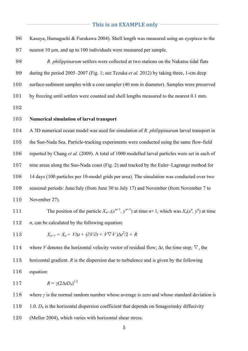
Kasuya, Hamaguchi & Furukawa 2004). Shell length was measured using an eyepiece to the 96

nearest 10 µm, and up to 100 individuals were measured per sample. 97

R. philippinarum settlers were collected at two stations on the Nakatsu tidal flats 98

during the period 2005–2007 (Fig. 1; see Tezuka et al. 2012) by taking three, 1-cm deep 99

surface-sediment samples with a core sampler (40 mm in diameter). Samples were preserved 100

by freezing until settlers were counted and shell lengths measured to the nearest 0.1 mm. 101

102

Numerical simulation of larval transport 103

A 3D numerical ocean model was used for simulation of R. philippinarum larval transport in 104

the Suo-Nada Sea. Particle-tracking experiments were conducted using the same flow-field 105

reported by Chang et al. (2009). A total of 1000 modelled larval particles were set in each of 106

nine areas along the Suo-Nada coast (Fig. 2) and tracked by the Euler–Lagrange method for 107

14 days (100 particles per 10-model grids per area). The simulation was conducted over two 108

seasonal periods: June/July (from June 30 to July 17) and November (from November 7 to 109

November 27). 110

The position of the particle Xn+1(xn+1, yn+1) at time n+1, which was Xn(xn, yn) at time 111

n, can be calculated by the following equation: 112

Xn+1 = Xn + VΔt + (∂V/∂t + V∇V )Δt2/2 + R 113

where V denotes the horizontal velocity vector of residual flow; Δt, the time step; ∇, the 114

horizontal gradient. R is the dispersion due to turbulence and is given by the following 115

equation: 116

R = γ(2ΔtDh)1/2 117

where γ is the normal random number whose average is zero and whose standard deviation is 118

1.0. Dh is the horizontal dispersion coefficient that depends on Smagorinsky diffusivity 119

(Mellor 2004), which varies with horizontal shear stress. 120

 This  is  an  EXAMPLE  only  

     

6

Vertical migration of larval particles was hypothesized as larvae were located at a 121

3-m depth from day 0 to day 11 but, then moved to 1 m above the ocean floor between day 122

12 and day 14. This assumption for the vertical migration of larval particles is based on 123

observational studies on the vertical distribution of larvae, including this study (see Results, 124

Fig. 6), which showed that smaller larvae (D- and umbo-shaped) were found at ~3 m, 125

whereas larger larvae (settling larvae) found in the bottom layer (Suzuki et al. 2002; Ishii, 126

Sekiguchi & Jinnai 2005; Kuroda 2005; Toba et al. 2012; Bidegain et al. 2013). The larval 127

stage was assumed to last 2 weeks (14 days) in this study, although it can vary with 128

temperature and food availability (Helm & Bourne 2004). 129

The larval retention rates, i.e., the ratio of larval particles remaining within the 130

Suo-Nada Sea, after the 14-day simulation were calculated as follows: 131

Retention rate after 14 days = 100 × Pa / P0 132

where Pa is the number of particles remaining within the Suo-Nada Sea after the 14-day 133

simulation, and P0 is the number of particles within the Suo-Nada Sea on Day 0. The 134

boundary of the Suo-Nada Sea was set on a line through two points (131.7°E, 33.7°N) and 135

(132.0°E, 34.0°N) (see Fig. 1), and particles located to the western side of the boundary line 136

were treated as inside the Suo-Nada Sea. Retention rates were calculated for each of the nine 137

areas where particles were released for two seasonal periods. 138

139

Results 140

141

Seasonal dynamics of larval distribution and settlement 142

Distribution of R. philippinarum larvae from April to November 2004–2007 is shown in Fig. 143

3. Seasonal changes in planktonic larval abundance are shown in Fig. 4. R. philippinarum 144

larvae were observed sporadically from April to November, with peak numbers being 145

 This  is  an  EXAMPLE  only  

     

7

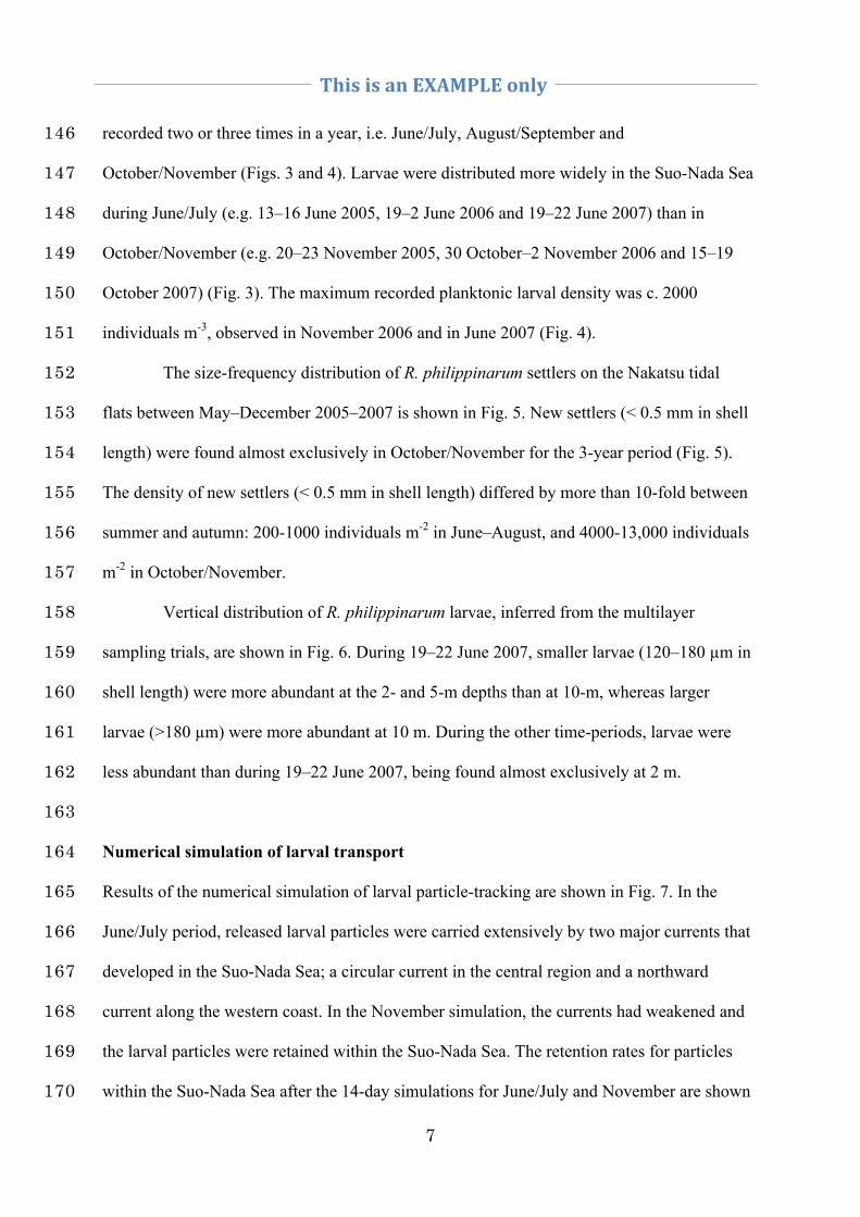
recorded two or three times in a year, i.e. June/July, August/September and 146

October/November (Figs. 3 and 4). Larvae were distributed more widely in the Suo-Nada Sea 147

during June/July (e.g. 13–16 June 2005, 19–2 June 2006 and 19–22 June 2007) than in 148

October/November (e.g. 20–23 November 2005, 30 October–2 November 2006 and 15–19 149

October 2007) (Fig. 3). The maximum recorded planktonic larval density was c. 2000 150

individuals m-3, observed in November 2006 and in June 2007 (Fig. 4). 151

The size-frequency distribution of R. philippinarum settlers on the Nakatsu tidal 152

flats between May–December 2005–2007 is shown in Fig. 5. New settlers (< 0.5 mm in shell 153

length) were found almost exclusively in October/November for the 3-year period (Fig. 5). 154

The density of new settlers (< 0.5 mm in shell length) differed by more than 10-fold between 155

summer and autumn: 200-1000 individuals m-2 in June–August, and 4000-13,000 individuals 156

m-2 in October/November. 157

Vertical distribution of R. philippinarum larvae, inferred from the multilayer 158

sampling trials, are shown in Fig. 6. During 19–22 June 2007, smaller larvae (120–180 µm in 159

shell length) were more abundant at the 2- and 5-m depths than at 10-m, whereas larger 160

larvae (>180 µm) were more abundant at 10 m. During the other time-periods, larvae were 161

less abundant than during 19–22 June 2007, being found almost exclusively at 2 m. 162

163

Numerical simulation of larval transport 164

Results of the numerical simulation of larval particle-tracking are shown in Fig. 7. In the 165

June/July period, released larval particles were carried extensively by two major currents that 166

developed in the Suo-Nada Sea; a circular current in the central region and a northward 167

current along the western coast. In the November simulation, the currents had weakened and 168

the larval particles were retained within the Suo-Nada Sea. The retention rates for particles 169

within the Suo-Nada Sea after the 14-day simulations for June/July and November are shown 170

 This  is  an  EXAMPLE  only  

     

8

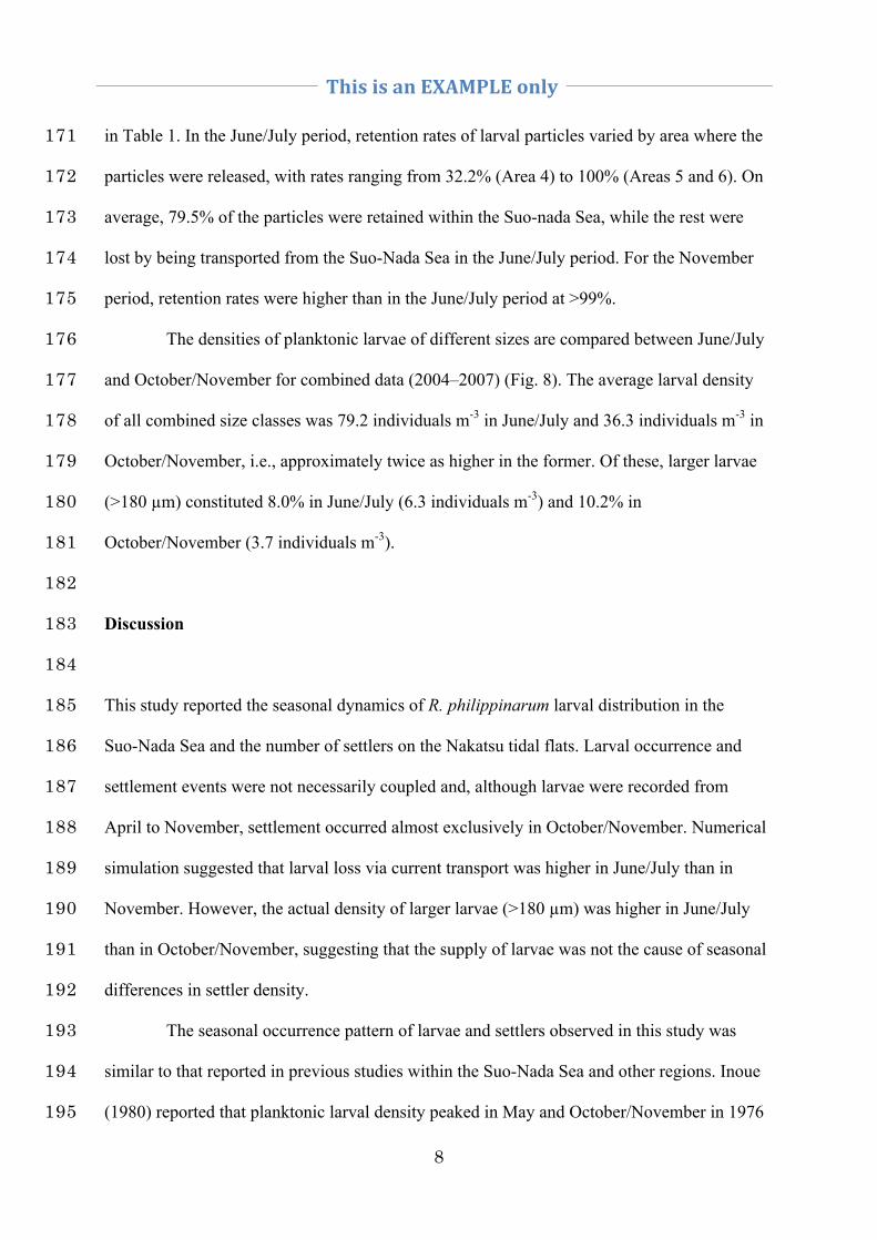
in Table 1. In the June/July period, retention rates of larval particles varied by area where the 171

particles were released, with rates ranging from 32.2% (Area 4) to 100% (Areas 5 and 6). On 172

average, 79.5% of the particles were retained within the Suo-nada Sea, while the rest were 173

lost by being transported from the Suo-Nada Sea in the June/July period. For the November 174

period, retention rates were higher than in the June/July period at >99%. 175

The densities of planktonic larvae of different sizes are compared between June/July 176

and October/November for combined data (2004–2007) (Fig. 8). The average larval density 177

of all combined size classes was 79.2 individuals m-3 in June/July and 36.3 individuals m-3 in 178

October/November, i.e., approximately twice as higher in the former. Of these, larger larvae 179

(>180 µm) constituted 8.0% in June/July (6.3 individuals m-3) and 10.2% in 180

October/November (3.7 individuals m-3). 181

182

Discussion 183

184

This study reported the seasonal dynamics of R. philippinarum larval distribution in the 185

Suo-Nada Sea and the number of settlers on the Nakatsu tidal flats. Larval occurrence and 186

settlement events were not necessarily coupled and, although larvae were recorded from 187

April to November, settlement occurred almost exclusively in October/November. Numerical 188

simulation suggested that larval loss via current transport was higher in June/July than in 189

November. However, the actual density of larger larvae (>180 µm) was higher in June/July 190

than in October/November, suggesting that the supply of larvae was not the cause of seasonal 191

differences in settler density. 192

The seasonal occurrence pattern of larvae and settlers observed in this study was 193

similar to that reported in previous studies within the Suo-Nada Sea and other regions. Inoue 194

(1980) reported that planktonic larval density peaked in May and October/November in 1976 195

 This  is  an  EXAMPLE  only  

     

9

on the northern coast of the Suo-Nada Sea (maximum larval density was 14,000 individuals 196

m-3 in October 1976), and that new settlers were found in abundance (26,700 individuals m-2 197

in November 1976) in October/November, but very few, new settlers were recorded in other 198

months. Fujimoto et al. (1985) observed that larval density peaked in April, June/July, 199

September and November during the period 1983–1984 on the southwest coast of the 200

Suo-Nada Sea, with a maximum density of 4550 individuals m-3 in November 1983 and 6140 201

individuals m-3 in April 1984 (larval density was calculated as the mean from eight sampling 202

stations). An increase in new settlers was observed in October/November 1983 (maximum of 203

350,000 individuals m-2 in November 1983) and in November/December 1984 (max, 20,000 204

individuals m-2). Although the maximum larval density observed in the current study was 205

lower than those recorded in the 1970s and 1980s, the seasonal pattern was consistent among 206

these studies. The difference in maximum larval density could be a result of differences in 207

the spawning biomass between the 2000s and the 1970–1980s; clam production in the 208

Suo-Nada Sea was 14,800 metric tonnes in 1976, 19,500–31,700 metric tonnes in 1983/1984, 209

and 94–780 metric tonnes during 2005–2007 (Ministry of Agriculture, Forestry and Fisheries, 210

Japan, 2012). Dense larval settlement in autumn has often been observed in other temperate 211

regions of Japan (Miyawaki & Sekiguchi 1999; Ishii et al. 2001; Toba et al. 2007). 212

The results of numerical simulation suggest that larval retention in the Suo-Nada Sea 213

should be higher, i.e., lower larval loss rates, in October/November than June/July, owing to 214

seasonal differences in the strength of two major currents in the Suo-Nada Sea. As 215

stratification developed in June/July, a circular current developed in the central region and a 216

northern current developed along the southwest coast of the Suo-Nada Sea. However, as 217

stratification declined in October/November, the currents weakened. The simulation 218

suggested that larval loss via transport from the Suo-Nada Sea was 20% in June/July and 0% 219

in October/November. However, this disparity could not explain the >10-fold difference in 220

 This  is  an  EXAMPLE  only  

     

10

settler density between October/November and June/August. Moreover, on average during 221

the period 2004–2007, the observed density of >180 µm larvae was higher in June/July than 222

in October/November. This suggests that, even if he larval loss via transport may be higher in 223

June/July, larval supply, as a result of spawning and larval loss via transport and mortality, 224

was not the limiting factor in June/July under the prevailing conditions. 225

Factors influencing settler density, other than larval supply, need to be considered, 226

and although not all factors were investigated in this study, several hypotheses may be 227

proposed. First, mortality during the critical period from settling to early post-settlement 228

affects settler density (Hunt & Scheibling 1997), and this mortality may be lower in 229

October/November than in other months. Predation and/or other factors, such as high 230

temperature in summer, may cause higher mortality in settling larvae or early settlers during 231

months other than October/November. Second, food availability for larvae may differ 232

seasonally, resulting in differences in mortality during settlement (Laing 1995; Tezuka et al. 233

2009). Third, the rate of larval settlement may vary due to seasonal differences in physical 234

conditions at settling sites, e.g., variation in sediment grain size (Tezuka et al. 2013). If a 235

suitable substrate is not found, larvae could delay settlement (Coon, Fitt & Bonar 1990) and, 236

as a result, become more prone to predation by benthic filter-feeders while drifting near the 237

bottom (Pineda et al. 2010). This study concentrated solely on larval settlement on the tidal 238

flats and other possible sites, e.g., subtidal areas, were not investigated. As such, settlement 239

failure on the tidal flats in seasons other than October/November needs to be investigated 240

further. 241

242

Acknowledgments 243

This research was funded by the Fisheries Agency, Japan. We thank Professor Takeoka and 244

Professor Guo from the Center for Marine Environmental Studies at Ehime University for 245

 This  is  an  EXAMPLE  only  

     

11

providing the ocean model outputs. We also thank reviewers and the editor for their 246

constructive and valuable comments, which helped us to improve the manuscript. 247

248

 This  is  an  EXAMPLE  only  

     

12

References 249

Bidegain G, Bárcena JF, García A & Juanes JA (2013) LARVAHS: Predicting clam larval 250

dispersal and recruitment using habitat suitability-based particle tracking model. 251

Ecological Modelling 268, 78–92. 252

Chang P-H, Guo X & Takeoka H (2009) A Numerical Study of the Seasonal Circulation in 253

the Seto Inland Sea, Japan. Journal of Oceanography 65, 721–736. 254

Coon SL, Fitt WK & Bonar DB (1990) Competence and delay metamorphosis in the Pacific 255

oyster Crassostrea gigas. Marine Biology 106, 379–387. 256

Dethier MN, Ruesink J, Berry H & Sprenger AG (2012) Decoupling of recruitment from 257

adult clam assemblages along an estuarine shoreline. Journal of Experimental Marine 258

Biology and Ecology 422-423, 48–54. 259

Drummond L, Mulcahy M & Culloty S (2006). The reproductive biology of the Manila clam, 260

Ruditapes philippinarum, from the North-West of Ireland. Aquaculture 254, 326–340. 261

Fujimoto T, Nakamura M, Kobayashi M, Hayashi I, Takiguchi K, Oda K & Ushima H 262

(1985) On the formation of the asari clam fishery ground. Annual Report of Fukuoka 263

Prefecture Buzen Fisheries Experimental Station S58, pp. 34–106. (In Japanese.) 264

Goulletquer P (1997) A Bibliography of the Manila Clam Tapes philippinarum. IFREMER, 265

La Tremblade, France. (RIDRV-97.021RN, 122 pp.) 266

Helm MM & Bourne N (2004) Hatchery culture of bivalves. A practical manual. Lovatelli A 267

(ed), FAO Fisheries Technical Paper 471. Rome, FAO. 177pp. 268

Hunt HL & Scheibling RE (1997) Role of early post-settlement mortality in recruitment of 269

benthic marine invertebrates. Marine Ecology Progress Series 155, 269–301. 270

Inoue Y (1980) On the ecology of the asari clam and the environment in Omi- and 271

Yamaguchi-wan sea. Fisheries Engineering 16, 29–35. (In Japanese.) 272

Ishii R, Sekiguchi H, Nakahara Y & Jinnai Y (2001) Larval recruitment of the manila clam 273

Ruditapes philippinarum in Ariake Sound, southern Japan. Fisheries Science 67, 274

 This  is  an  EXAMPLE  only  

     

13

579–591. 275

Ishii R, Sekiguchi H, Jinnai Y (2005) Vertical distributions of larvae of the clam Ruditapes 276

philippinarum and the striped horse mussel Musculista senhousia in eastern Ariake 277

Bay, southern Japan. Journal of Oceanography 61, 973–978. 278

Kasuya T, Hamaguchi M & Furukawa K (2004) Detailed observation of spatioal abundance 279

of clam larvae Ruditapes philippinarum in Tokyo Bay, central Japan. Journal of 280

Oceanography 60, 631–636. 281

Kuroda N (2005) Larval transportation and settlement mechanism to tidal flat in Japanese 282

littleneck clam Ruditapes philippinarum. Bulletin of Fisheries Research Agency, 283

Supplement 3, 67–77. (In Japanese with English abstract.) 284

Laing I (1995) Effect of food supply on oyster spatfall. Aquaculture 131, 315–324. 285

Matsumura T, Okamoto S, Kuroda N & Hamaguchi M (2001) Temporal and spatial 286

distributions of planktonic larvae of the clam Ruditapes philippinarum in Mikawa 287

Bay; Application of an immunofluorescence identification method. Japanese Journal 288

of Benthology 56, 1–8. (In Japanese with English abstract.) 289

Mellor G (2004) Users guide for a three-dimensional, primitive equation, numerical ocean 290

model (the June 2004 revision). Program in Atmospheric and Oceanic Sciences, 291

Princeton University, Princeton, NJ 08544-0710, 1–56. 292

Ministry of Agriculture, Forestry and Fisheries, Japan (2012) Annual report of statistics on 293

fisheries and aquaculture production in 2010. Nourin Toukei Kyoukai, Tokyo. (In 294

Japanese.) 295

Miyawaki D & Sekiguchi H (1999) Interannual variation of bivalve populations on temperate 296

tidal flats. Fisheries Science 65, 817–829. 297

Pineda J, Hare JA & Sponaugle S (2007) Larval transport and dispersal in the coastal ocean 298

and consequences for population connectivity. Oceanography 20, 22–39. 299

Pineda J, Porri F, Starczak V & Blythe J (2010) Causes of decoupling between larval supply 300

 This  is  an  EXAMPLE  only  

     

14

and settlement and consequences for understanding recruitment and population 301

connectivity. Journal of Experimental Marine Biology and Ecology 392, 9–21. 302

Shanks AL & Brink L (2005) Upwelling, downwelling, and cross-shelf transport of bivalve 303

larvae: test of a hypothesis. Marine Ecology Progress Series 302, 1–12. 304

Suzuki T, Ichikawa T & Momoi M (2002) The approach to predict sources of pelagic bivalve 305

larvae supplied to tidal flat areas by receptor mode model: a modeling study 306

conducted in Mikawa Bay. Bulletin of the Japanese Society of Fisheries 307

Oceanography 2, 88–101. (In Japanese with English abstract.) 308

Tamaki A, Nakaoka A, Maekawa H & Yamada F (2008) Spatial partitioning between species 309

of the phytoplankton-feeding guild on an estuarine intertidal sand flat and its 310

implication on habitat carrying capacity. Estuarine, Coastal and Shelf Science 78, 311

727–738. 312

Tezuka N, Ichisaki E, Kanematsu M, Usuki H, Hamaguchi M & Iseki K (2009) Particle 313

retention efficiency of asari clam Ruditapes philippinarum larvae. Aquatic Biology 6, 314

281–287. 315

Tezuka N, Kamimura S, Hamaguchi M, Saito H, Iwano H, Egashira J, Fukuda Y, 316

Tawaratsumida T, Nagamoto A & Nakagawa K (2012) Settlement, mortality and 317

growth of the asari clam (Ruditapes philippinarum) for a collapsed population on a 318

tidal flat in Nakatsu, Japan. Journal of Sea Research 69, 23–35. 319

Tezuka N, Kanematsu M, Asami K, Sakiyama K, Hamaguchi M & Usuki H (2013) Effect of 320

salinity and substrate grain size on larval settlement of the asari clam (Manila clam, 321

Ruditapes philippinarum). Journal of Experimental Marine Biology and Ecology 439, 322

108–112. 323

Tezuka N, Kanematsu M, Asami K, Nakagawa N, Shigeta T, Uchida M & Usuki H (2014) 324

Ruditapes philippinarum mortality and growth under netting treatments in a 325

population-collapsed habitat. Coastal Ecosystems 1, 1–13. 326

 This  is  an  EXAMPLE  only  

     

15

Toba M, Yamakawa H, Kobayashi Y, Sugiura Y, Honma K & Yamada H (2007) 327

Observations on the maintenance mechanisms of metapopulations, with special 328

reference to the early reproductive process of the Manila clam Ruditapes 329

philippinarum (Adams & Reeve) in Tokyo Bay. Journal of Shellfish Research 26, 330

121–130. 331

Toba M, Yamakawa H, Shoji N & Kobayashi Y (2012) Vertical distribution of Manila clam 332

Ruditapes philippinarum larvae characterized through year-round observations in 333

Tokyo Bay, Japan. Nippon Suisan Gakkaishi 78, 1135–1148. (In Japanese with 334

English abstract.) 335

Young EF, Bigg GR, Grant A, Walker P & Brown J (1998) A modelling study of 336

environmental influence on bivalve settlement in the Wash, England. Marine Ecology 337

Progress Series 172, 197–214. 338

339

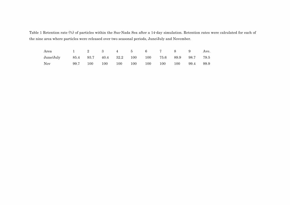
Table 1 Retention rate (%) of particles within the Suo-Nada Sea after a 14-day simulation. Retention rates were calculated for each of the nine area where particles were released over two seasonal periods, June/July and November.

Area 1 2 3 4 5 6 7 8 9 Ave. June/July 85.4 93.7 40.4 32.2 100 100 75.6 89.9 98.7 79.5 Nov 99.7 100 100 100 100 100 100 100 99.4 99.9

 This  is  an  EXAMPLE  only  

     

16

Figure legends 340

341

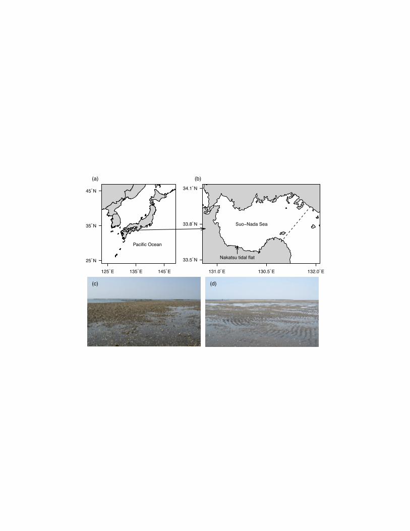
Fig. 1 (a)-(b), Map of the Suo-Nada Sea, Japan. Dashed line in (b) is the boundary used to 342

calculate the larval retention rate (see text). (c)-(d), Nakatsu tidal flats where larval settlement 343

was recorded. 344

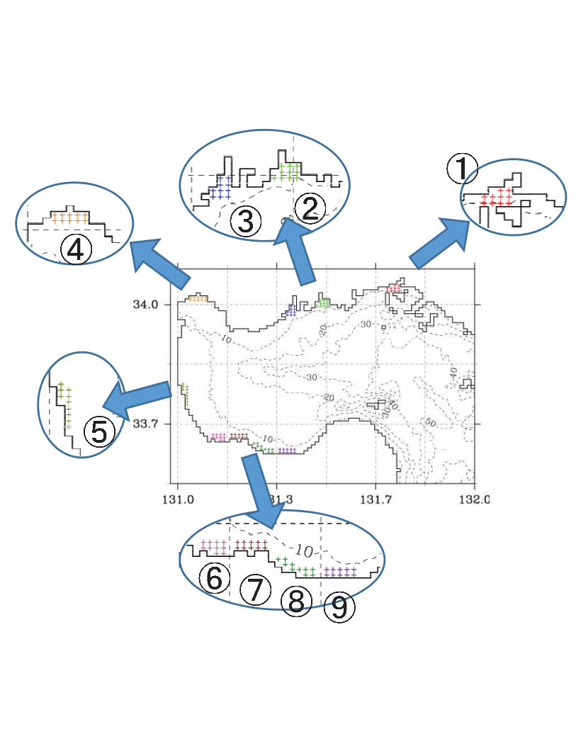
Fig. 2 Modelled larval particles were set in nine areas along the Suo-Nada Sea coast for 345

numerical simulation of Ruditapes philippinarum larval transport. A total of 1000 modeled 346

larval particles were set on 10-model grids in each area. The model grids in each area were 347

indicated as “+” symbols with identical color. 348

(other figures not shown in this example) 349

125 E゚ 135 E゚ 145 E゚

25 N゚

35 N゚

45 N゚

Pacific Ocean

(a)

131.0 E゚ 130.5 E゚ 132.0 E゚

33.5 N゚

33.8 N゚

34.1 N゚

Suo−Nada Sea

Nakatsu tidal flat

(b)

(c) (d)