introduction - Caltech Authors

3.0 INTRODUCTION

The silica glass fiber has become the most important transmission medium for long-distance, high-data-rate optical communication. It has caused what can be called with very little exaggeration a revolution in the art and practice of communication. This success is due mostly to the prediction [1] and realization [2] of low-loss fibers and to the ability to drastically reduce group velocity dispersion in such fibers so that extremely short optical pulses (~5 × 10-12 s) undergo minimal spreading in propagation. Confined and lossless propagation in fibers is accomplished by total reflection from the dielectric interface between the core and the cladding. This requires that the index of refraction of the core be greater than that of the cladding. In this chapter we will investigate the mode characteristics of the circular dielectric waveguide. Both step-index waveguides and graded-index fibers will be analyzed. The exact hybrid modes of the step-index waveguide will be derived first, to be followed by a treatment of the linearly polarized mode, which is a very useful approximation. The Wentzel-Kramers-Brillouin (WKB) method is used to derive the approximate solution of the field and the propagation constants of the graded-index fibers. Modal dispersion, chromatic dispersion, and fiber attenuation are also dicussed.

1Major contributions to this chapter were made by P. Yeh.

74

3Propagation of

Optical Beams

in Fibers1

WAVE EQUATIONS IN CYLINDRICAL COORDINATES 75

3.1 WAVE EQUATIONS IN CYLINDRICAL COORDINATES

Since the refractive index profiles n(r) of most fibers are cylindrically symmetric, it is convenient to use the cylindrical coordinate system. The field components are Er, Eφ, Ez, Hφ, Hr, and Hz. The wave equation (2.4-3) assumes its simple form only for the Cartesian components of the field vectors. Since the unit vectors ar and aφ are not constant vectors, the wave equations involving the transverse components are very complicated. The wave equation for the z component of the field vectors, however, remains simple,

(3.1-1)

where k2 = ω2n2∕c2 and ∇2 is the Laplacian operator given by

The problems of wave propagation in a cylindrical structure are usually approached by solving for Ez and Hz first and then expressing Er, Eφ, Hr, and Hφ in terms of Ez and Hz.

Since we are concerned with the propagation along the waveguide, we assume

(3.1-2)

i.e., every component of the field vector assumes the same z- and t-dependence of exp[i(ωt - βz)]. Maxwell’s equations (3.1-1) and (3.1-2) are now written in terms of the cylindrical components and are given, respectively, by

and

(3.1-3a)

(3.1-4c)

(3.1-3b)

(3.1-3c)

(3.1-4a)

(3.1-4b)

76 PROPAGATION OF OPTICAL BEAMS IN FIBERS

Using (3.1-3a), (3.1-3b), (3.1-4a), and (3.1-4b), we can solve for Er, Eφ, Hr, and Hφ in terms of Ez and Hz. The results are

(3.1-5)

(3.1-6)

These relations show that it is sufficient to determine Ez and Hz in order to specify uniquely the wave solution. The remaining components can be calculated from (3.1-5) and (3.1-6).

With the assumed z-dependence of (3.1-2), the wave equation (3.1-1) becomes

This equation is separable, and the solution takes the form

(3.1-8)

where l = 0, 1, 2, 3, . . . , so that Ez and Hz are single-valued functions of Φ. Then (3.1-7) becomes

(3.1-9)

where ψ = Ez, Hz.Equation (3.1-9) is the Bessel differential equation, and the solutions are

called Bessel functions of order l. If k2 - β2 > 0, the general solution of (3.1-9) is

(3.1-10)

where h2 = k2 - β2, c1 and c2 are constants, and Jl, Yl are Bessel functions of the first and second kind, respectively, of order l. If k2 - β2 < 0, the general solution of (3.1-9) is

(3.1-11)

where q2 = β2 - k2, c1 and c2 are constants, and Il, Kl are the modified Bessel functions of the first and second kind, respectively, of order l.

(3.1-7)

THE STEP-INDEX CIRCULAR WAVEGUIDE 77

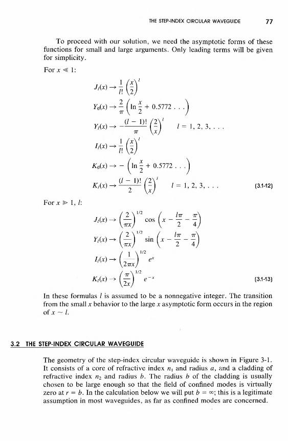
To proceed with our solution, we need the asymptotic forms of these functions for small and large arguments. Only leading terms will be given for simplicity.

For x ≪ 1 :

For x ≫ 1, l:

(3.1-12)

(3.1-13)

In these formulas l is assumed to be a nonnegative integer. The transition from the small x behavior to the large x asymptotic form occurs in the region of x ~ l.

The geometry of the step-index circular waveguide is shown in Figure 3-1. It consists of a core of refractive index n1 and radius a, and a cladding of refractive index n2 and radius b. The radius b of the cladding is usually chosen to be large enough so that the field of confined modes is virtually zero at r = b. In the calculation below we will put b = ∞; this is a legitimate assumption in most waveguides, as far as confined modes are concerned.

3.2 THE STEP-INDEX CIRCULAR WAVEGUIDE


The radial dependence of the fields Ez and Hz is given by (3.1-10) or (3.1-11), depending on the sign of k2 - β2. For confined propagation, β must be larger than n2ω∕c (i.e., β > n2k0 = n2ω∕c). This ensures that the wave is evanescent in the cladding region, r > a. The solution is thus given by (3.1-11) with c1 = 0. This is evident from the asymptotic behavior for large r given by (3.1-13). The evanescent decay of the field also ensures that the power flow is along the direction of the z axis, i.e., no radial power flow exists. Thus the fields of a confined mode in the cladding (r > a) are given by

Figure 3-1 Structure and index profile of a step-index circular waveguide.

(3.2-1)

where C and D are two arbitrary constants, and q is given by

(3.2-2)

For the fields in the core, r < a, we must consider the behavior of the fields as r → 0. According to (3.1-12), Yl and Kl are divergent as r → 0. Since the fields must remain finite at r = 0, the proper choice for the fields in the core (r < a) is (3.1-10) with c2 = 0. This becomes evident only when matching, at the interface r = a, the tangential components of the field vectors E and H in the core with the cladding field components derived from (3.2-1); we


are unable to accomplish this if the radial dependence of the core fields is given by Il. Thus the propagation constant β must be less than n1k0, and the core fields are given by

(3.2-6)

(3.2-7)

(3.2-3)

where A and B are two arbitrary constants, and h is given by

(3.2-4)

In the field expressions (3.2-1) and (3.2-3), we have taken a "+" sign in front of lφ in the exponents. A negative sign would yield a set of independent solutions, but with the same radial dependence. Physically, l plays a role similar to the quantum number describing the z component of the orbital angular momentum of an electron in a cylindrically symmetric potential field. Thus, if the positive sign in front of lφ corresponds to a clockwise “circulation” of photons about the z axis, the negative sign would correspond to a counterclockwise "circulation" of photons around the axis. Since the fiber itself does not possess any preferred sense of rotation, these two states are degenerate.

Equations (3.2-1) and (3.2-3) together require that h2 > 0 and q2 > 0, which translates to

(3.2-5)

which can be regarded as a necessary condition for confined modes to exist. This is identical to the condition discussed in Section 13.1 for the slab dielectric waveguide and can be expected on intuitive grounds from our discussions of total internal reflection at a dielectric interface.

Using (3.2-1) and (3.2-3) in conjunction with (3.1-5) and (3.1-6), we can calculate all the field components in both the cladding and the core regions. The result is

Core (r < a):


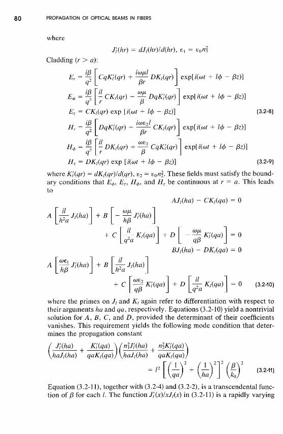
where

Cladding (r > a):

(3.2-8)

(3.2-9)

where K'l(qr) = dKl(qr)/d(qr), ε2 = ε0n22. These fields must satisfy the boundary conditions that Eφ, Ez, Hφ, and Hz be continuous at r = a. This leads to

(3.2-10)

where the primes on Jl and Kl again refer to differentiation with respect to their arguments ha and qa, respectively. Equations (3.2-10) yield a nontrivial solution for A, B, C, and D, provided the determinant of their coefficients vanishes. This requirement yields the following mode condition that deter- mines the propagation constant

Equation (3.2-11), together with (3.2-4) and (3.2-2), is a transcendental function of β for each l. The function J'l(x)∕xJl(x) in (3.2-11) is a rapidly varying

(3.2-11)


oscillatory function of x = ha. Therefore, (3.2-11) may be considered roughly as a quadratic equation in J'l(ha)∕haJl(ha). For a given l and a given frequency ω, only a finite number of eigenvalues β can be found that satisfy (3.2-11) and (3.2-5). Once the eigenvalues have been found, we employ (3.2-10) to solve for the ratios B/A, C/A, and D/A that determine the six field components of the mode corresponding to each propagation constant β. These ratios are, from (3.2-10),

(3.2-12)

The quantity B/A is of particular interest because it is a measure of the relative amount of Ez and Hz in a mode (i.e., B/A = Hz/Ez). Note that Ez and Hz are out of phase by π∕2.

Mode Characteristics and Cutoff Conditions

In the treatment of slab waveguide modes in Section 13.2, we found that the solutions are easily separated into two classes, the TE and TM modes. In the circular waveguide, the solutions also separate into two classes. However, these are not in general TE or TM, each having in general nonvanishing Ez, Hz, Eφ, Hφ, Er, and Hr components. The two classes in solutions can be obtained by noting that (3.2-11) is quadratic in J'l(ha)/haJl(ha), and when we solve for this quantity, we obtain two different equations corresponding to the two roots of the quadratic equation. The eigenvalues resulting from these two equations yield the two classes of solutions that are designated con- ventionally as the EH and HE modes.

By solving equation (3.2-11) for J'l(ha)/haJl(ha), we obtain

(3.2-13)

where the arguments of K'l and Kl are qa. We now use the Bessel function relations

(3.2-14)


and (3.2-13) becomes

EH modes:

(3.2-15a)

HE modes:

(3.2-15b)

where

(3.2-16)

Equation (3.2-15) can be solved graphically by plotting both sides as functions of ha, letting (qa)2 = (n21 - n22)k2α20 - (ha)2 on the right-hand side.

We consider first the special case when l = 0. At l = 0 we have ∂∕∂φ = 0, and all the field components of the modes are radially symmetric. There are two families of solutions that correspond to (3.2-15a) and (3.2-15b) above. In the first case, the mode condition (3.2-15a) becomes

(3.2-17a)

where we used K'0(x) = -K1(x). Under condition (3.2-17a), the constants A and C vanish according to (3.2-10) or (3.2-12). By substituting A = C = 0 and l = 0 in equations (3.2-6) through (3.2-9), we find that the only nonvanishing field components are Hr, Hz, and Eφ. These solutions are thus referred to as TE modes. If the eignevalues are βm, m = 1, 2, 3, . . . , the TE modes are designated as TE0m, m = 1, 2, 3, . . . , where the first subscript is l = 0.

In the second case, the mode condition (3.2-15b) at l = 0 becomes

(3.2-17b)

where we used K'0(x) = -K1(x) and J-1(x) = -J1(x). In this case the constants B and D vanish according to (3.2-10) or (3.2-12). By substituting B = D = 0 and l = 0 in equations (3.2-6) through (3.2-9), we find that the only nonvanishing field components are Er, Ez, and Hφ. These solutions are thus referred to as TM modes and are designated as TM0m.

Now consider the graphical solution of (3.2-17a) and (3.2-17b). Confined modes require that q be real to achieve the exponential decay of the field in the cladding. Thus we need only consider ha in the range 0 ≤ ha ≤ V ≡ k0a(n21 - n22)1/2. The right-hand sides of (3.2-17) are always negative. Starting from -K1(V)∕VK0( V) for TE modes at ha = 0, the right side of (3.2-17a) is


which diverges to -∞ at ha = V. The right side of (3.2-l7b) for TM modes behaves identically except for a factor of n22∕n21. On the left sides of (3.2-l7a) and (3.2-l7b), J1(ha)∕haJ0(ha) starts from 1/2 at ha = 0 and increases monotonically until it diverges to ∞ at ha = 2.405, which is the first zero of J0(ha). Beyond ha = 2.405, J1(ha)/haJ0(ha) varies from -∞ to +∞ between the zeros of J0(ha). For large values of ha, J1(ha)∕haJ0(ha) is a function resembling -(ha)-1 tan(ha - π∕4), according to Figure 3-2 which shows the two curves describing the right and left sides of (3.2-l7a), respectively. The normalized frequency V = k0a(n21 - n22)1/2 is assumed to be high enough so that two modes, marked by the circles at the intersection of the two curves, exist. The vertical asymptotes are given by the roots of J0(ha) = 0. If the maximum value of ha, (ha)max = V, is smaller than the first root of J0(x), 2.405, there can be no intersection of the two curves for real β. If V is between the first and the second zero of J0(x), there will be exactly one

Figure 3-2 Graphical determination of the propagation constants of TE modes (l = 0) for a step-index waveguide.

a monotonically decreasing function of ha and becomes asymptotical, according to (3.1-12)

(3.2-18)


intersection of the two curves. Thus the cutoff value (a∕λ) for TE0m (or TM0m) waves is given by

Figure 3-3 Graphical determination of the propagation constants of l = 1 EH modes for a step-index fiber.

(3.2-19)

where x0m is the mth zero of J0(x). The first three zeros are

For higher zeros, the asymptotic formula

gives adequate accuracy (to at least three figures).When l ≠ 0 in equations (3.2-15), the modes are no longer TE or TM

but become the EH or HE modes of the waveguide. These can still be solved graphically in a manner similar to that outlined for the l = 0 case. For l = 1, the two curves representing the two sides of the EH mode condition (3.2-l5a) are shown in Figure 3-3. The normalized frequency V = k0a(n21 - n22)1/2 is assumed to be 8, so that there are two intersections. These are the EH11 and EH12 modes. The vertical asymptotes are given by the roots of J1(x) = 0. Figure 3-4 shows those of the HE modes. At the same value of


Figure 3-4 Graphical determination of the propagation constants of the l = 1 HE modes for a step-index dielectric waveguide.

V = 8 there are three intersections that correspond to HE11, HE12, and HE13 modes, respectively. The vertical asymptotes are also given by the roots of J1(x) = 0. Note that, as shown in Figure 3-4, the intersection for HE11 mode always exists regardless of the value of V. This means the HE11 mode does not have a cutoff. All other HE1m, EH1m modes have cutoff values of a∕λ given by

(3.2-20)

where m' = m for EH1m modes and m' = m - 1 for HE1m modes; x1m is the mth zero of J1(x), excluding the one at x = 0. The first three zeros are

For higher zeros, the asymptotic formula

gives adequate accuracy (to at least three figures). For l > 1, the cutoff


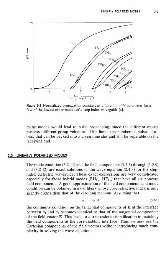
as a function of V = k0a(n21 - n22)1/2; here k0 = ω∕c. Since the phase velocity of a mode is ω∕β, n is the ratio of the speed of light in vacuum to the mode phase velocity (n is also called the effective mode index). Figure 3-5 shows n for a number of the low-order modes of the step-index circular waveguide [4]. We note that at cutoff, each mode has a value of (β∕k0) = n2. We can easily understand this by recalling that as the mode approaches cutoff, the fields extend well into the cladding layer. Thus, near cutoff the modes are poorly confined and most of the energy propagates in medium 2 and thus n = n2. By similar reasoning, for frequencies far above cutoff, the mode is tightly confined to the core, and n approaches n1.

As discussed earlier, for V < 2.405, only the fundamental HE11 mode can propagate. This is an important result, since for many applications single mode propagation is required. These applications include interferometry that calls for well-defined stationary phase fronts and optical communications by transmission of very short optical pulses. In the latter case the excitation of

values for a/λ are given by [3]

(3.2-21)

(3.2-22)

where xlm is the mth zero of Jl(x) = 0, and zlm is the mth root of

(3.2-23)

If we substitute the propagation constant β for l > 1 into (3.2-12), we find that B/A is neither zero nor infinite. This means that both Ez and Hz are present in these modes. The designation of these hybrid modes is based on the relative contribution of Ez and Hz to a transverse component (e.g., Er or Eφ) of the field at some reference point. If Ez makes the larger contribution, the mode is considered E-like and designated EHlm, and so on. The mode HE11 can propagate at any wavelength, as noted earlier, since (a∕λ)HE11 = 0. The next modes that can propagate, according to (3.2-19) are the TE01 and TM01 modes. Since xlm or zlm forms an increasing sequence for fixed l and increasing m, or for fixed m and increasing l, the number of allowed modes increases as the square of a/λ (see Problem 3.1).

For many applications, the important characteristic of a mode is the propagation constant β as a function of the frequency ω (or normalized frequency V). This information is often presented as the mode index of the confined mode

(3.2-24)

LINEARLY POLARIZED MODES 87

Figure 3-5 Normalized propagation constant as a function of V parameter for a few of the lowest-order modes of a step-index waveguide [4].

many modes would lead to pulse broadening, since the different modes possess different group velocities. This limits the number of pulses, i.e., bits, that can be packed into a given time slot and still be separable on the receiving end.

The mode condition (3.2-11) and the field components (3.2-6) through (3.2-9) and (3.2-12) are exact solutions of the wave equation (2.4-3) for the step- index dielectric waveguide. These exact expressions are very complicated especially for those hybrid modes (EHlm, HElm) that have all six nonzero field components. A good approximation of the field components and mode condition can be obtained in most fibers whose core refractive index is only slightly higher than that of the cladding medium. Assuming that

(3.3-1)

the continuity condition on the tangential components of H at the interface between n1 and n2 becomes identical to that of the tangential components of the field vector E. This leads to a tremendous simplification in matching the field components at the core-cladding interface. Thus we may use the Cartesian components of the field vectors without introducing much complexity in solving the wave equation.

3.3 LINEARLY POLARIZED MODES


This simplified solution of the linearly polarized modes for the round fiber using the assumption (3.3-1) is due to Gloge [5]. In the limit (3.3-1), all the transverse wave numbers (h, q) are much smaller compared to the propagation constant β, i.e.,

(3.3-4)

The longitudinal component of the electric field vector E is related to Hx, according to the Maxwell equation ▽ × H = ε ∂E∕∂t

(3.3-7)

where we used (3.3-6) in arriving at the last equality. We note that the field components Ex and Hy are zero in this solution. The other four field components can be expressed in terms of Ey. In order to calculate Hz and Ez, we need to carry out the differentiation with respect to x and y, respectively, according to (3.3-6) and (3.3-7). Since Ey is of the form (3.3-5), we need the relations

(3.3-8)

(3.3-2)

We now start by solving the wave equation for the transverse Cartesian field components Ex, Ey, Hx, and Hy. These field components also satisfy the wave equations (3.1-7) and (3.1-9). For a step-index dielectric waveguide, the general solutions are given by (3.1-10) and (3.1-11). We now look for solutions where either the x or y component of the electric field vanishes. Since Eφ can be expressed in terms of Ex and Ey as

(3.3-3)

it is apparent that Eφ component is simply proportional to either Ex or Ey. Thus the continuity of Eφ becomes equivalent to the continuity of Ex or Ey in these new solutions. Take the E field of a y-polarized solution of the form

(3.3-5)

where A and B are constants. We assume that Ez ≪ Ey. The magnetic field components are then given, according to (2.4-1) and (3.1-2), by

(3.3-6)


and

we obtain the following expressions for the field components.

Core (r < a):

(3.3-9)

By using the definition of r and φ

(3.3-10)

(3.3-11)

we obtain

(3.3-12)

(3.3-13)

(3.3-14)

and

(3.3-15)

We now substitute (3.3-5) for Ey in (3.3-6) and (3.3-7) and carry out the differentiation, using equations (3.3-8) through (3.3-15). After some laborious algebra and using the following functional relations of the Bessel function,

(3.3-16)

(3.3-17)

(3.3-18)


Cladding (r > a):

(3.3-20)

to ensure the continuity of Ey(Eφ ∝ Ey) at the core boundary r = a. The constant A is then determined by the normalization condition.

The field solution (3.3-18) and (3.3-19) is a y-polarized wave (Ex = 0). For a complete field description, we also need the mode with the orthogonal polarization (i.e., an x-polarized wave). The field components Ex and Ey of this orthogonal mode are taken of the form

(3.3-21)

(3.3-22)

and the other field components are, according to the Maxwell equations,

where we have assumed that Ez ≪ Ex. We note that Ey = 0 and Hx ≃ 0 in this solution. By substituting (3.3-21) for Ex in (3.3-23) and carrying out the differentiation, using equations (3.3-8) through (3.3-15), we obtain, again

(3.3-19)

In arriving at (3.3-18) and (3.3-19), we have also used β = n1k0 ≃ n2k0, since n2k0 < β < n1k0 and n2 → n1. Note that Ey and Hx are the dominant field components because in the limit (3.3-1) h, q ≪ β. In other words, the field is essentially transverse. The constant B is given by

(3.3-23)


In arriving at (3.3-24) and 3.3-25), we again made the assumption that β ≃ n1k0 ≃ n2k0 because of (3.3-1). We note that Ex and Hy are the dominant field components in this solution. Therefore, the mode is again nearly transverse and linearly polarized along the x direction. The constant B is again given by (3.3-20) to ensure the continuity of Ex(Eφ ∝ Ex) at the core boundary r = a.

We have obtained the field expressions for two types of guided modes whose transverse fields are polarized orthogonally to each other. These field expressions are approximate solutions of Maxwell's equations, provided the tangential components of the field vectors are continuous at the dielectric interface r = a. The continuity of Eφ at r = a leads to B = AJl(ha)/Kl(qa) (3.3-20). The Hφ components are proportional to the Eφ components, according to the field expressions (3.3-18), (3.3-19), (3.3-24), and (3.3-25) in this approximation. Therefore the continuity of Eφ results in the continuity of Hφ.

after some laborious algebra and using the relations (3.3-16) and (3.3-17), the following expressions for the field amplitudes:

Core (r < a):

(3.3-24)

Cladding (r > a):

(3.3-25)


We now consider the continuity of Ez at r = a. Since the continuity condition must hold for all azimuth angles φ, we must equate the coefficients of exp[i(l + 1)φ] and exp[i(l - 1)φ] separately. Using the field expressions (3.3-18) and (3.3-19) and (3.3-20), we obtain the following mode conditions:

(3.3-26)

and

(3.3-27)

The same equations result from the continuity of Hz. In addition, if we use the field expressions (3.3-24) and (3.3-25) for the x-polarized mode, we will arrive at the same mode conditions (3.3-26) and (3.3-27). This means that these two transversely orthogonal modes are degenerate in the propagation constant β. The mode condition (3.3-27) is mathematically equivalent to (3.3-26) if we use the recurrence relation of the Bessel functions (3.3-17).

The mode condition (3.3-26) obtained in this approximation is much simpler than the exact expression (3.2-11). The exact mode condition (3.2-11) has twice as many solutions as the simple one (3.3-26) because (3.2-11) is quadratic in J'l/Jl. This indicates that each solution of (3.3-26) is really twofold degenerate. In fact the propagation constants of the exact HEl+1,m and EHl-1,m modes are nearly degenerate [6]. They become exactly the same in the limit n1 → n2. This can also be seen from the expressions of the field components Ez and Hz in (3.3-18), (3.3-19), (3.3-24), and (3.3-25). Comparison of the linearly polarized mode expressions with the exact modes (3.2-3) shows that the linearly polarized modes are actually a superposition of HEl+1,m and EHl+1,m modes [6]. Two independent linear superpositions lead to the x- polarized and y-polarized modes. The total number of modes is the same in both theories. The eigenvalues obtained from (3.3-26) are labeled as βlm with l = 0, 1, 2, 3, . . . , m = 1, 2, 3, . . . , where the subscript m indicates the mth root of the transcendental equation (3.3-26). The modes are designated LPlm. The lowest-order mode HE11 now has the propagation constant labeled β01 and the mode designated LP01.

The mode conditions for those linearly polarized waves (3.3-26) or (3.3-27) can also be solved graphically. Figure 3-6 shows the normalized propagation constant as a function of the normalized frequency V. The mode cutoff corresponds to the condition q = 0 which, according to (3.3-27), leads to the condition

(3.3-28)

where

(3.3-29)


Figure 3-6 Normalized propagation constant b as function of normalized frequency V for the guided modes of the optical fiber, b = (β/kc - n2)/(n1 — n2). (After Reference [5].)

It follows that the lowest-order mode, characterized by l = 0, has a cutoff given by the lowest root of the equation

Table 3-1 Cutoff Values of V for Some Low- Order LP Modes

V m = 1 m = 2 m = 3 m = 4

l = 0 0 3.832 7.016 10.173l = 1 2.405 5.520 8.654 11.792l = 2 3.832 7.016 10.173 13.323l = 3 5.136 8.417 11.620 14.796l = 4 6.379 9.760 13.017 16.224

(3.3-30)

Hence V = 0. In other words, the lowest-order mode does not have a cutoff. This is the HE11 mode and is now labeled LP01. The next mode of the type l = 0, cuts off when J1(V) next equals zero, that is, when V = 3.832. This mode is labeled LP02. The cutoff values of V for some low-order LPlm modes are given in Table 3-1. All these values are zeros of the Bessel function. For


Figure 3-7 The regions of the parameter V for modes of order l = 0, 1.

Figure 3-8 Sketch of the fiber cross section and the four possible distributions of LP11.


Figure 3-7 shows the regions in which a given mode is the highest one allowed for a given l value group, labeled in LP mode designation. Also shown in the figure are the associated HE, EH, TE, and TM mode notations that are the exact modes. Figure 3-8 shows the field distribution of the LP11 modes [6]. The LP01 mode has radially symmetric field distribution J0(hr) in the core.

One of the most important advantages of using the linearly polarized mode is that the modes are almost transversely polarized and are dominated by one transverse electric field component (Ex or Ey) and one transverse magnetic field component (Hy or Hx). The E vector can be chosen to be along any arbitrary radial direction with the H vector along a perpendicular radial direction. Once this mode is chosen, there exists another independent mode with E and H orthogonal to the first pair.

Power Flow and Power Density

We now derive expressions for the Poynting vector and the power flow in the core and cladding. The time-averaged Poynting vector along the waveguide is, acccording to (3.1-18)

Substituting the field components from (3.3-18) and (3.3-19) or (3.3-24) and (3.3-25) into (3.3-32), we obtain

(3.3-33)

Note that the intensity distribution is cylindrical symmetric (i.e., no φ- dependence). The amount of power that is contained in the core and the cladding is given by, respectively,

high-order modes, the cutoff value of V is given approximately according to (3.3-28) and (3.1-13)

(3.3-31)

(3.3-32)

(3.3-34)

(3.3-35)


Using the following integrals of Bessel functions [7]

the powers Pcore and Pclad can be written, respectively,

(3.3-36a)

By using (3.3-20) for B and the mode conditions (3.3-26) and (3.3-27), the power Pclad can be written

Figure 3-9 Fractional power contained in the cladding as a function of the frequency parameter V. (After Reference [5].)

(3.3-36b)

(3.3-37)

(3.3-38)

(3.3-39)

For those ha values that are allowed by the mode condition (3.3-26) or (3.3-27), Jl-1(ha)Jl+1(ha) is always negative, so that Pclad is always positive. The negativeness of Jl-1(ha)Jl+1(ha) can be seen from (3.3-26) and (3.3-27), since the Kl(qa)'s are always positive. According to (3.3-37) and (3.3-39),


the total power flow is thus given by

(3.3-40)

The ratio of cladding power to the total power, Γ2 = (Pclad/P), which measures the fraction of mode power flowing in the cladding layer, is given, according to (3.3-39) and (3.3-40), by

(3.3-41)

where we used (ha)2 + (qa)2 = k20a2(n21 - n22) = V2. Figure 3-9 shows the ratio Pclad/P for several modes as a function of the normalized frequency V [5]. Note that the fundamental mode LP01 is best confined. Generally speak- ing, Pclad/P increases when the mode subscript lm increases.

Mode Dispersion

The propagation constant of a guided mode LPlm is obtained as a solution of the mode condition (3.3-26) or (3.3-27). It is often expressed in terms of the mode index defined as

(3.3-42)

where the mode index nlm (often called effective index of mode lm) is considered as a function of n1, n2, and ω (see Figure 3-6). The velocity with which the mode energy in a light pulse travels down a waveguide is called the group velocity and is characterized by the expression

(3.3-43)

At a given frequency, different modes will thus have different group velocities. This is the modal dispersion discussed in Section 2.9. Pulse broadening and distortion in multimode waveguides where the energy is carried simul- taneously by many modes is due mostly to modal dispersion, i.e., lm- dependence of vg.

In single-mode waveguides (.e.g, LP01 mode l = 0, m = 1), modal dispersion is not operative, and the pulse broadening is caused by the group velocity dispersion alone. Dropping the subscript lm = 01, the group velocity in a single-mode step-index fiber can be written as

(3.3-44)

where n1 is the refractive index of the core, n2 is the refractive index of the cladding, and n is the mode index. The first two terms in the square bracket


are the contribution from material dispersion, whereas the third term is a result of the waveguide dispersion. From the uniform dielectric perturbation theory, the change in the eigenvalue β2 results from a uniform dielectric perturbation δn21, and δn22 in the core and cladding, respectively, is given by

where Γ1 and Γ2 are the fraction of power flowing in the core and cladding, respectively. Using β2 = n2(ω/c)2, we obtain from (3.3-45)

(3.3-46)

The group velocity can thus be expressed as

where we put a subscript w to indicate that (∂n/∂ω)w is a waveguide dispersion. In a weakly guiding fiber n1 ≃ n2, we may assume that

(3.3-48)

where the subscript m indicates material dispersion. The group velocity (3.3-47) can thus be written

Using ω = 2πc/λ, (3.3-49) can be written in terms of λ as

(3.3-49)

(3.3-50)

The group velocity dispersion D is thus given, according to (2.9-33) and (3.3-49), by

(3.3-51)

Note that both material dispersion and waveguide dispersion contribute to the group velocity dispersion. The second-order derivatives (∂2n/∂λ2)m,w vanish at the point of inflection on the curve n(λ), i.e., point where (∂n/∂λ)m,w is minimum or maximum. For GeO2-doped silica, (∂2n/∂λ2)m passes through zero near λ = 1.3 μm [8, 9]. The waveguide dispersion (∂2n/∂λ2)w vanishes at a wavelength that depends on core diameter a as well as n1 and n2. It is possible to tailor the zero-dispersion wavelength in single-mode fibers by

(3.3-45)

(3.3-47)

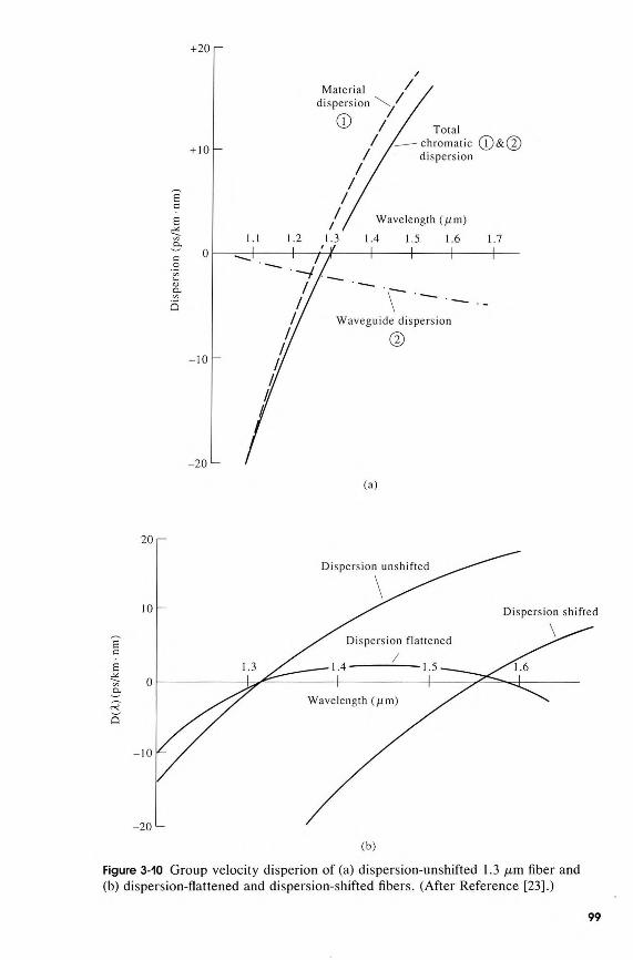
Figure 3-10 Group velocity disperion of (a) dispersion-unshifted 1.3 μm fiber and(b) dispersion-flattened and dispersion-shifted fibers. (After Reference [23].)

99

100 PROPAGATION OF OPTICAL BEAMS 1N FIBERS

balancing the (negative) material dispersion against the (positive) waveguide dispersion [10]. Thus, by choosing a core diameter a between 4 and 5 μm and relative refractive index difference of (n1 - n2)/n1 > 0.004, the wavelength of minimum group velocity dispersion can be shifted to the 1.5- to 1.6-μm region where the loss is lowest [11-16]. Figure 3-10(a) shows the waveguide and material (chromatic) contributions to the group velocity dispersion of the "conventional" 1.3 μm fibers. Figure 3-10(b) plots the dispersion curves for dispersion-shifted fibers.

3.4 GRADED-INDEX FIBERS

Referring to Figure 3-11, we now consider a circular waveguide in which the index of refraction of the core is graded. An example of such a core medium is the quadratic-index medium discussed in Chapter 2. Graded-index fibers are used in some applications because they offer a multimode propagation in a relatively large core fiber coupled with low modal dispersion. Consider the case of a power-law refractive index profile given by

(3.4-1)

where Δ = (n21 - n22)/2n1 ≃ (n1 - n2)/n1 and g is the power-law coefficient. The case of g = 2 is known as the parabolic-index profile, and is the quadratic- index medium discussed in Chapter 2. In the limit when g → ∞, the index profile becomes that of a step-index waveguide.

It was shown in Chapter 2 [see Table 2-1(6)] that light rays follow sinusoidally varying curved paths in the quadratic-index medium (g = 2). Rays that do not approach the core boundary closely can be regarded as propa- gating in an idealized, infinitely extended graded-index medium, as indicated by the dashed lines in Figure 3-11. For those rays, the mode analysis of such fibers is greatly simplified by assuming that the graded-index profile of the

Figure 3-11 Structures and index profile of a graded-index fiber.

GRADED-INDEX FIBERS 101

core continues indefinitely beyond the core region. For example, in the quadratic-index fiber [with g = 2 in (3.4-1)], the mode soIutions are Her- mite-Gaussian functions in a Cartesian coordinate (see Chapter 2) or La- guerre-Gaussian functions in cylindrical coordinates, provided the index profile continues its quadratic shape beyond r = a. For those well-confined modes that have most of their mode power flowing in the core region (r < a), it is a good approximation to assume that the index profile retains the same radial dependence beyond r = a. Even in this approximation, closed form solutions of the mode amplitudes can only be obtained for very few refractive index profiles. In general, only approximate solutions for the mode functions or the propagation constants can be obtained. One of the most powerful analytical methods for obtaining the approximate mode solutions and the propagation constants of graded-index fibers with arbitrary profiles is the WKB method. This method provides a good approximation for the mode amplitudes and the propagation constants whenever the index of refraction n(r) does not vary appreciably over distances on the order of one wavelength. In what follows we will present some important results of the WKB approximation that are useful in deriving the propagation constants. For the detailed derivation of these results, the reader is referred to Ref- erences [16-18].

The WKB Approximation

In the approximate WKB solution that follows, we take the transverse component of the linearly polarized electric field of the (LP) modes as

where the direction of the magnetic field is perpendicular to the electric field and in such a sense that gives a positive power flow in the z direction. The radial function ψ(r) obeys Equation (3.1-9), which is now written as

(3.4-4)

where

(3.4-5)

p(r) may be interpreted as the local transverse wave number at r. The solution to the wave equation (3.4-4) is oscillatory in the region where p2(r) > 0 and becomes exponential in the region where p2(r) < 0. For confined modes,

(3.4-2)

The transverse component of the magnetic field is given by

(3.4-3)


p2(r = ∞) must be negative to ensure the exponential decay of the field and p2(r) > 0 in some region in order to have a finite field at r = 0. Let r1 and r2 define a region r1 < r < r2 where p2(r) > 0, and let p2(r) < 0 elsewhere. For l = 0, r1 = 0, and p2(r2) = 0. For l ≠ 0, r1 > 0, and p2(r1) = p2(r2) = 0. In the regions outside the range r1 < r < r2, the wave is evanescent. These regions are "classically inaccessible," and light is totally reflected from the surfaces r = r1 and r = r2.

We now take ψ(r) of the form

(3.4-7)

where the prime indicates differentiation with respect to r. If we assume S" + S'/r ≪ S'2, we obtain the first approximation for S'

This approximation is valid, provided

(3.4-8)

(3.4-9)

By substituting (3.4-8) for S' in the first two terms in (3.4-7), we obtain the second approximation for S'

From (3.4-6) and (3.4-12), the general solution ψ(r) thus takes the form

(3.4-13)

where c1 and c2 are arbitrary constants. This solution (3.4-13) is not valid at the turning points where p(r) = 0 because at these points the assumption

(3.4-6)

where S(r) is a complex function of r. Substitution of (3.4-6) for ψ(r) in (3.4-4) leads to

(3.4-10)

Using (3.4-9), S' can be written

(3.4-11)

Integration of (3.4-11) leads to

(3.4-12)

GRADED-INDEX FIBERS 103

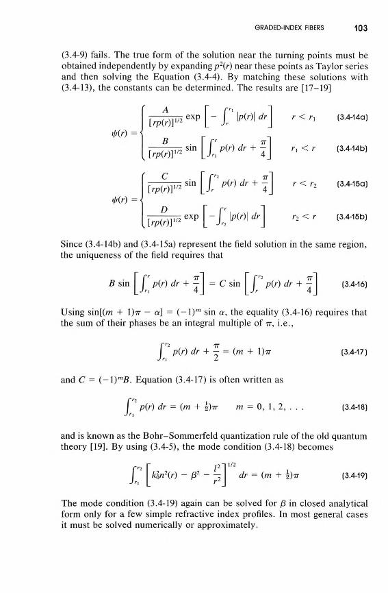
(3.4-9) fails. The true form of the solution near the turning points must be obtained independently by expanding p2(r) near these points as Taylor series and then solving the Equation (3.4-4). By matching these solutions with (3.4-13), the constants can be determined. The results are [17-19]

(3.4-14a)

(3.4-15a)

Since (3.4-14b) and (3.4-15a) represent the field solution in the same region, the uniqueness of the field requires that

Using sin[(m + 1)π - α] = (-1)m sin α, the equality (3.4-16) requires that the sum of their phases be an integral multiple of π, i.e.,

(3.4-17)

and C = (-1)mB. Equation (3.4-17) is often written as

(3.4-18)

The mode condition (3.4-19) again can be solved for β in closed analytical form only for a few simple refractive index profiles. In most general cases it must be solved numerically or approximately.

(3.4-15b)

(3.4-16)

and is known as the Bohr-Sommerfeld quantization rule of the old quantum theory [19]. By using (3.4-5), the mode condition (3.4-18) becomes

(3.4-19)

(3.4-14b)


Example: WKB Solutions for the Propagation Constants of Quadratic-Index Fiber

We consider a fiber with parabolic-index profile

Substituting n(r) into the mode condition (3.4-19), we obtain

(3.4-20)

(3.4-21)

where r1 and r2 are roots of p2(r) = 0 (i.e., the turning points). Using the substitution u = r2 and the integral formula

(3.4-22)

The mode condition (3.4-21) becomes

Solving (3.4-23) for β, we obtain

(3.4-24)

The WKB value (3.4-24) of the propagation constant β of the quadratic- index fiber modes is identical to that given by the exact solution of the wave equation (2.9-13). In using (3.4-24) we must keep in mind that (3.4-24) is obtained by assuming an index profile of the form (3.4-20) for all r. In practice the parabolic-index profile is truncated at the core boundary r = a. Therefore, a confined mode must have its propagation constant larger than n1(1 - 2Δ)1/2k0 (i.e., n1(1 - 2Δ)1/2k0 < β < n1k0). Thus the mode subscripts (quantum numbers) l and m are limited by the following condition:

(3.4-25)

where n2 is the clad refractive index n2 = n1(1 - 2Δ)1/2. Note that this n2 is not to be confused with n2 defined in Chapter 2 [Equation (2.9-1a)].

Probably the single most important factor responsible for the emergence of the silica glass optical fiber as a premium transmission medium is the low optical propagation losses in such fibers. Figure 3-12 shows the measured

(3.4-23)

3.5 ATTENUATION IN SILICA FIBERS

PROBLEMS 105

Figure 3-12 Observed loss spectrum of a germanosilicate single-mode fiber. Estimated loss spectra for various intrinsic materials effects and waveguide imperfections are also shown. (From Reference [20].)

losses as a function of wavelength of a high-quality, germania-doped single- mode fiber. The loss peak around 1.4 μm is due to residual OH contamination of the glass. A low value of loss ~0.2 dB/km obtains near λ = 1.55 μm. Consequently, this region of the spectrum is now favored for long-distance optical communication. Recent experiments have taken advantage of the small pulse spreading near the zero group velocity dispersion wavelength and the low losses to demonstrate high-data-rate transmission (data rate exceeding 400 Mb/s) over a propagation path exceeding 100 km [20, 21] at λ ~ 1.55 μm.

For a more detailed discussion of propagation effects in optical fibers, the student can consult Reference [22].

Problems

3.1 The number of confined modes that can be supported by a circular dielectric waveguide depends on the refractive-index profile and the wavelength.

a. Using the cutoff value for the LPlm mode, show that the mode subscripts (l, m) for a step-index fiber must satisfy the condition


where V = k0a(n21 — n22)1/2. Show that each LPlm mode is fourfold degenerate.

b. By counting the allowed mode subscripts (l, m), show that the total number of confined modes that can be supported by a step-index fiber is

Show that this expression again agrees with the results obtained in (b) for step-index fibers (g = ∞) and in (c) for quadratic-index fibers (g = 2).

3.2 The numerical aperture (NA) is a measure of the light-gathering capa- bility of a fiber. It is defined as the sine of the maximum external angle of the entrance ray (measured with respect to the axis of fiber) that is trapped in the core by total internal reflection.

a. Show that

c. Using (3.4-25) show that for a truncated quadratic-index fiber

Note that the total number of modes in a truncated quadratic-index fiber is one-half of that of a step-index fiber.

d. Estimate the number of confined modes in a multimode step-index fiber with a = 50 μm, n1 = 1.52, n2 = 1.50 at a carrier wavelength of λ = 1 μm.

e. In a general, truncated graded-index fiber with a core radius a and a cladding index n2, it is convenient to define an effective V number such that

and the number of confined modes is approximately given by

Show that this approximation agrees with (b) and (c) for step-index and quadratic-index fibers, respectively.

f. Show that, according to (e), the number of confined modes in a power- law graded-index fiber with an index profile given by (3.4-1) is

b. Show that the solid acceptance angle in air is

PROBLEMS 107

c. Show that the solid angle (in air) for a single electromagnetic radiation mode leaving or entering the core aperture is

where 2 accounts for the two independent polarizations in air. Show that this estimate agrees with Problem 3.1.

e. Find the numerical aperture of a multimode fiber with n1 = 1.52 and N2 = 1.50.

3.3 A single-mode step-index fiber must have a V number less than 2.405; i.e.,

d. The total number of modes the fiber can support, couple to, and radiate into air is therefore

a. Show that the expression derived in Problem 3.1(b) (N ≃ 4V2/π2) still applies, provided we realize that a single-mode fiber supports two independently polarized HE01 modes (or LP01 modes).

b. With a = 5 μm, n2 = 1.50, and λ = 1 μm, find the maximum core index for a single-mode fiber. (Answer: n1 = 1.50195.)

c. With n1 = 1.501, n2 = 1.500, and λ = 1 μm, find the maximum core radius for a single-mode fiber. (Answer: a = 7 μm.)

d. Show that the confinement factor for a single-mode fiber is

where ha satisfies the mode condition (3.3-26)

e. Show that, by using the table of Bessel functions, ha = 1.647 is an approximate solution to the mode condition for V = 2.405. Evaluate the confinement factor Γ1 for the LP01 mode of this single-mode fiber (Answer: Γ1 = 83%). Note that this is the maximum confinement factor for a single- mode fiber. Compare this value with the curves in Figure 3-9.

3.4 Mode condition

a. Derive the mode condition for step-index fibers (3.2-11).b. Derive the expressions for the constants B, C, D, in terms of A (3.2-12).


c. Derive the mode conditions for TE and TM modes (3.2-17).d. Show that Ez = Er = 0 for TE modes and Hz = Hr = 0 for TM modes.e. Show that in the limit n1 - n2 ≪ n1, TE and TM modes become identical.

3.5

a. Derive (3.3-6) and (3.3-7).b. Derive (3.3-18) and (3.3-19).c. Derive (3.3-23).d. Derive (3.3-24) and (3.3-25).

References

1. Kao, C. K., and T. W. Davies, "Spectroscopic studies of ultra low loss optical glasses," J. Sci. Instrum. 1(no. 2): 1063, 1968.

2. Kapron, F. P., D. B. Keck, and R. D. Maurer, "Radiation losses in glass optical waveguides," Appl. Phys. Lett. 17:423, 1970.

3. Snitzer, E., "Cylindrical dielectric waveguide modes," J. Opt. Soc. Am. 51:491, 1961.

4. Keck, D. B., Fundamentals in Optical Fiber Communications (M. K. Barnoski, ed.). New York: Academic Press, 1976, Chapter 1.

5. G1oge, D., "Weakly guiding fibers," Appl. Opt. 10:2252, 1971.6. See, for example, D. Marcuse, Theory of Dielectric Optical Waveguides.

New York: Academic Press, 1974.7. See, for example, I. S. Gradshteyn and I. M. Ryzhik, Table of Integrals,

Series, and Products. New York: Academic Press, 1965, p. 634, Eq. (5.54-2).

8. Payne, D. N., and W. A. Gambling, "Zero material dispersion in optical fibers," Electron. Lett. 11:176, 1975.

9. Cohen, L. G., and C. Lin, "Pulse delay measurements in the zero material dispersion wavelength region for optical fibers," Appl. Opt. 12:3136, 1977.

10. Li, T., "Structures, parameters, and transmission properties of optical fibers," Proc. IEEE 68:1175, 1980.

11. Cohen, L. G., W. L. Mammel, and H. M. Presby, "Correlation between numerical predications and measurements of single-mode fiber dispersion characteristics," Appl. Opt. 19:2007, 1980.

12. Tsuchiya, H., and N. Imoto, "Dispersion-free single mode fibers in 1.5 μm wavelength region," Electron. Lett. 15:476, 1979.

13. Cohen, L. G., C. Lin, and W. G. French, "Tailoring zero chromatic dispersion into the 1.5-1.6 μm low-loss spectral region of single-mode fibers," Electron. Lett. 15:334, 1979.

14. White, K. I., and B. P. Nelson, "Zero total dispersion in step-index monomode fibres at 1.30 and 1.55 m," Electron. Lett. 15:396, 1979.

15. Gambling, W. A., H. Matsumara, and C. M. Ragdale, "Zero total dispersion in graded-index single-mode fibers," Electron. Lett. 15:474, 1979.

REFERENCES 109

16. Yamada, J. L, et al., "High speed optical pulse transmission at 1.29 μm wavelength using low loss single mode fibers," IEEE J. Quantum Electron. QE-14:791, 1978.

17. Morse, P. M., and H. Feshbach, Methods of Theoretical Physics. New York: McGraw-Hill, 1953.

18. Mathews, J., and R. L. Walker, Mathematical Methods of Physics. New York: Benjamin, 1965.

19. Landau, L. D., and E. M. Lifshitz, Quantum Mechanics. London: Pergamon Press, 1958.

20. Miya, T., Y. Terunuma, T. Hosaka, and T. Miyashita, "Ultimate low- loss single-mode fiber at 1.55 μm," Electron. Lett. 15:106, 1979.

21. Suematsu, Y., "Long wavelength optical fiber communication," Proc. IEEE 71:692, 1983.

22. Miller, S., and I. P. Kaminow, ed., Optical Fiber Telecommunication IL San Diego: Academic Press, 1988, Chapters 2 and 3.

23. Figure 3-10(a) is courtesy of S. R. Nagel, AT&T Bell Laboratories. Figure 3-10(b) is from D. L. Frazen, "Single mode fiber measurements," Proceedings of the Tutorial Sessions Conference on Optical Fiber Communications. Washington, D.C., Opt. Soc. Am., 1988, p. 101.

introduction - Caltech Authors

Documents

Transcript of introduction - Caltech Authors