Power Systems Analysis - Caltech Computer Science

Lecture Notes for EE/CS/EST 135

Power Systems AnalysisA Mathematical Approach

Steven H. Low

CMS, EE, [email protected]

December 29, 2012February 6, 2014April 26, 2015 (Zhejiang University)October 2015 (Skoltech)January 2017January 2018January 2019July 2019 (Melbourne University)March 2020

These are draft lecture notes. Corrections, comments, questions will be appreciated - please send them [email protected]

Contents

1 Introduction 1

1.1 Notations . . . . . . . . . . . . . . . . . . . . . . . . . . . . . . . . . . . . . . . . . . . 1

1.2 Units . . . . . . . . . . . . . . . . . . . . . . . . . . . . . . . . . . . . . . . . . . . . . . 2

I Component models 4

2 Basic concepts 5

2.1 Phasor representation . . . . . . . . . . . . . . . . . . . . . . . . . . . . . . . . . . . . . 5

2.1.1 Voltage and current phasors . . . . . . . . . . . . . . . . . . . . . . . . . . . . . 5

2.1.2 Impedances . . . . . . . . . . . . . . . . . . . . . . . . . . . . . . . . . . . . . . 6

2.2 Balanced three-phase systems . . . . . . . . . . . . . . . . . . . . . . . . . . . . . . . . 8

2.2.1 Balanced systems in Wye configuration . . . . . . . . . . . . . . . . . . . . . . . 8

2.2.2 Balanced systems in Delta configuration . . . . . . . . . . . . . . . . . . . . . . . 17

2.2.3 Delta and Wye transformation . . . . . . . . . . . . . . . . . . . . . . . . . . . . 20

2.2.4 Per-phase analysis . . . . . . . . . . . . . . . . . . . . . . . . . . . . . . . . . . 22

2.2.5 Example configurations and line limits . . . . . . . . . . . . . . . . . . . . . . . 24

2.3 Complex power . . . . . . . . . . . . . . . . . . . . . . . . . . . . . . . . . . . . . . . . 29

2.3.1 Single-phase power . . . . . . . . . . . . . . . . . . . . . . . . . . . . . . . . . . 29

2.3.2 Three-phase power . . . . . . . . . . . . . . . . . . . . . . . . . . . . . . . . . . 32

2.3.3 Advantages of three-phase power . . . . . . . . . . . . . . . . . . . . . . . . . . 33

2.4 Bibliographical notes . . . . . . . . . . . . . . . . . . . . . . . . . . . . . . . . . . . . . 36

2.5 Problems . . . . . . . . . . . . . . . . . . . . . . . . . . . . . . . . . . . . . . . . . . . 36

2

3 Transmission line models 50

3.1 Line characteristics . . . . . . . . . . . . . . . . . . . . . . . . . . . . . . . . . . . . . . 50

3.1.1 Series resistance r and shunt conductance g . . . . . . . . . . . . . . . . . . . . . 50

3.1.2 Series inductance l . . . . . . . . . . . . . . . . . . . . . . . . . . . . . . . . . . 51

3.1.3 Shunt capacitance c . . . . . . . . . . . . . . . . . . . . . . . . . . . . . . . . . . 53

3.1.4 Balanced three-phase line . . . . . . . . . . . . . . . . . . . . . . . . . . . . . . 54

3.2 Line models . . . . . . . . . . . . . . . . . . . . . . . . . . . . . . . . . . . . . . . . . . 56

3.2.1 Transmission matrix . . . . . . . . . . . . . . . . . . . . . . . . . . . . . . . . . 56

3.2.2 Lumped-circuit P model . . . . . . . . . . . . . . . . . . . . . . . . . . . . . . . 60

3.2.3 Real and reactive line losses . . . . . . . . . . . . . . . . . . . . . . . . . . . . . 61

3.2.4 Lossless line . . . . . . . . . . . . . . . . . . . . . . . . . . . . . . . . . . . . . 62

3.2.5 Short line . . . . . . . . . . . . . . . . . . . . . . . . . . . . . . . . . . . . . . . 65

3.3 Appendix: solution of (3.7) . . . . . . . . . . . . . . . . . . . . . . . . . . . . . . . . . . 68


3.5 Problems . . . . . . . . . . . . . . . . . . . . . . . . . . . . . . . . . . . . . . . . . . . 69

4 Transformer models 82

4.1 Single-phase transformer . . . . . . . . . . . . . . . . . . . . . . . . . . . . . . . . . . . 82

4.1.1 Ideal transformer . . . . . . . . . . . . . . . . . . . . . . . . . . . . . . . . . . . 82

4.1.2 Equivalent circuit . . . . . . . . . . . . . . . . . . . . . . . . . . . . . . . . . . . 83

4.2 Three-phase transformer . . . . . . . . . . . . . . . . . . . . . . . . . . . . . . . . . . . 87

4.2.1 Ideal transformer . . . . . . . . . . . . . . . . . . . . . . . . . . . . . . . . . . . 87

4.2.2 Equivalent circuit . . . . . . . . . . . . . . . . . . . . . . . . . . . . . . . . . . . 93

4.3 Equivalent impedance in transformer circuit . . . . . . . . . . . . . . . . . . . . . . . . . 95

4.3.1 Transmission matrix . . . . . . . . . . . . . . . . . . . . . . . . . . . . . . . . . 96

4.3.2 Driving-point impedance . . . . . . . . . . . . . . . . . . . . . . . . . . . . . . . 98

4.4 Per-phase analysis . . . . . . . . . . . . . . . . . . . . . . . . . . . . . . . . . . . . . . . 101

4.4.1 Analysis procedure . . . . . . . . . . . . . . . . . . . . . . . . . . . . . . . . . . 102

4.4.2 Normal systems . . . . . . . . . . . . . . . . . . . . . . . . . . . . . . . . . . . . 106

4.5 Per-unit normalization . . . . . . . . . . . . . . . . . . . . . . . . . . . . . . . . . . . . 110

4.5.1 Kirchhoff’s laws . . . . . . . . . . . . . . . . . . . . . . . . . . . . . . . . . . . 111

4.5.2 Across ideal transformer . . . . . . . . . . . . . . . . . . . . . . . . . . . . . . . 111

4.5.3 Off-nominal transformers . . . . . . . . . . . . . . . . . . . . . . . . . . . . . . 114

4.5.4 Three-phase quantities . . . . . . . . . . . . . . . . . . . . . . . . . . . . . . . . 116

4.5.5 Per-unit per-phase analysis . . . . . . . . . . . . . . . . . . . . . . . . . . . . . . 119


4.7 Problems . . . . . . . . . . . . . . . . . . . . . . . . . . . . . . . . . . . . . . . . . . . 120

5 Generator models 140

5.1 Simple round-rotor model . . . . . . . . . . . . . . . . . . . . . . . . . . . . . . . . . . . 140

5.2 Two-reaction model . . . . . . . . . . . . . . . . . . . . . . . . . . . . . . . . . . . . . . 141

6 Distribution system models 142

6.1 Distribution lines . . . . . . . . . . . . . . . . . . . . . . . . . . . . . . . . . . . . . . . 142

6.2 Distribution transformers . . . . . . . . . . . . . . . . . . . . . . . . . . . . . . . . . . . 142

6.3 Voltage regulators . . . . . . . . . . . . . . . . . . . . . . . . . . . . . . . . . . . . . . . 142

6.3.1 Two-winding autotransformer . . . . . . . . . . . . . . . . . . . . . . . . . . . . 142

6.3.2 Step-voltage regulator . . . . . . . . . . . . . . . . . . . . . . . . . . . . . . . . 148

6.3.3 Power flow analysis . . . . . . . . . . . . . . . . . . . . . . . . . . . . . . . . . 154

6.3.4 Three-phase voltage regulator . . . . . . . . . . . . . . . . . . . . . . . . . . . . 156

6.3.5 Volt/var control . . . . . . . . . . . . . . . . . . . . . . . . . . . . . . . . . . . . 156

6.4 Shunt capacitors . . . . . . . . . . . . . . . . . . . . . . . . . . . . . . . . . . . . . . . . 158

6.5 Other devices . . . . . . . . . . . . . . . . . . . . . . . . . . . . . . . . . . . . . . . . . 158


6.7 Problems . . . . . . . . . . . . . . . . . . . . . . . . . . . . . . . . . . . . . . . . . . . 158

II Network models 160

7 Bus injection models 161

7.1 Bus admittance matrix Y . . . . . . . . . . . . . . . . . . . . . . . . . . . . . . . . . . . 161

7.1.1 Notations . . . . . . . . . . . . . . . . . . . . . . . . . . . . . . . . . . . . . . . 161

7.1.2 Power system components . . . . . . . . . . . . . . . . . . . . . . . . . . . . . . 162

7.1.3 General network . . . . . . . . . . . . . . . . . . . . . . . . . . . . . . . . . . . 168

7.1.4 Kron reduction . . . . . . . . . . . . . . . . . . . . . . . . . . . . . . . . . . . . 170

7.1.5 Solving I = YV . . . . . . . . . . . . . . . . . . . . . . . . . . . . . . . . . . . . 171

7.1.6 Invertibility of Y . . . . . . . . . . . . . . . . . . . . . . . . . . . . . . . . . . . 173

7.1.7 Summary . . . . . . . . . . . . . . . . . . . . . . . . . . . . . . . . . . . . . . . 179

7.2 Power flow models . . . . . . . . . . . . . . . . . . . . . . . . . . . . . . . . . . . . . . 180

7.2.1 Complex form . . . . . . . . . . . . . . . . . . . . . . . . . . . . . . . . . . . . 180

7.2.2 Polar form . . . . . . . . . . . . . . . . . . . . . . . . . . . . . . . . . . . . . . 182

7.2.3 Cartesian form . . . . . . . . . . . . . . . . . . . . . . . . . . . . . . . . . . . . 182

7.2.4 Types of buses . . . . . . . . . . . . . . . . . . . . . . . . . . . . . . . . . . . . 183

7.3 Properties of power flow solutions . . . . . . . . . . . . . . . . . . . . . . . . . . . . . . 183

7.3.1 Voltage collapse . . . . . . . . . . . . . . . . . . . . . . . . . . . . . . . . . . . 183

7.4 Computation methods . . . . . . . . . . . . . . . . . . . . . . . . . . . . . . . . . . . . . 184

7.4.1 Gauss-Seidel algorithm . . . . . . . . . . . . . . . . . . . . . . . . . . . . . . . . 184

7.4.2 Newton-Raphson algorithm . . . . . . . . . . . . . . . . . . . . . . . . . . . . . 185

7.4.3 Fast decoupled algorithm . . . . . . . . . . . . . . . . . . . . . . . . . . . . . . . 189


7.6 Problems . . . . . . . . . . . . . . . . . . . . . . . . . . . . . . . . . . . . . . . . . . . 190

8 Branch flow models 201

8.1 General network . . . . . . . . . . . . . . . . . . . . . . . . . . . . . . . . . . . . . . . . 201

8.2 Radial networks . . . . . . . . . . . . . . . . . . . . . . . . . . . . . . . . . . . . . . . . 203

8.2.1 With line shunts . . . . . . . . . . . . . . . . . . . . . . . . . . . . . . . . . . . 204

8.2.2 Without line shunts . . . . . . . . . . . . . . . . . . . . . . . . . . . . . . . . . . 205

8.3 Equivalence . . . . . . . . . . . . . . . . . . . . . . . . . . . . . . . . . . . . . . . . . . 207

8.4 Linear approximations and bounds . . . . . . . . . . . . . . . . . . . . . . . . . . . . . . 210

8.5 Power flow solutions . . . . . . . . . . . . . . . . . . . . . . . . . . . . . . . . . . . . . 212

8.5.1 Backward forward sweep . . . . . . . . . . . . . . . . . . . . . . . . . . . . . . . 212


8.7 Problems . . . . . . . . . . . . . . . . . . . . . . . . . . . . . . . . . . . . . . . . . . . 214

9 Linear models 219

9.1 DC power flow model . . . . . . . . . . . . . . . . . . . . . . . . . . . . . . . . . . . . . 219

9.2 Laplacian matrix L . . . . . . . . . . . . . . . . . . . . . . . . . . . . . . . . . . . . . . 221

9.3 Linear models for radial networks . . . . . . . . . . . . . . . . . . . . . . . . . . . . . . 224

9.4 Application: topology identification . . . . . . . . . . . . . . . . . . . . . . . . . . . . . 224

9.5 Problems . . . . . . . . . . . . . . . . . . . . . . . . . . . . . . . . . . . . . . . . . . . 224

10 Unbalanced multiphase network 229

10.1 Introduction . . . . . . . . . . . . . . . . . . . . . . . . . . . . . . . . . . . . . . . . . . 229

10.2 Component models . . . . . . . . . . . . . . . . . . . . . . . . . . . . . . . . . . . . . . 229

10.2.1 Three-phase lines . . . . . . . . . . . . . . . . . . . . . . . . . . . . . . . . . . . 230

10.2.2 Impedance loads in Y configuration . . . . . . . . . . . . . . . . . . . . . . . . . 233

10.2.3 Impedance loads in D configuration . . . . . . . . . . . . . . . . . . . . . . . . . 234

10.3 Single-phase equivalent circuit . . . . . . . . . . . . . . . . . . . . . . . . . . . . . . . . 236

10.3.1 Bus admittance matrix Y . . . . . . . . . . . . . . . . . . . . . . . . . . . . . . . 236

10.3.2 Power flow model . . . . . . . . . . . . . . . . . . . . . . . . . . . . . . . . . . 239

10.3.3 OPF and semidefinite relaxation . . . . . . . . . . . . . . . . . . . . . . . . . . . 239

10.4 Symmetrical components and sequence networks . . . . . . . . . . . . . . . . . . . . . . 241

10.4.1 Symmetric components . . . . . . . . . . . . . . . . . . . . . . . . . . . . . . . . 242

10.4.2 Power in sequence networks . . . . . . . . . . . . . . . . . . . . . . . . . . . . . 244

10.4.3 Sequence network of three-phase lines . . . . . . . . . . . . . . . . . . . . . . . . 245

10.4.4 Sequence network of impedance loads in Y configuration . . . . . . . . . . . . . . 246

10.4.5 Sequence network of impedance loads in D configuration . . . . . . . . . . . . . . 247

10.4.6 Sequence network of transformers . . . . . . . . . . . . . . . . . . . . . . . . . . 249

10.4.7 Sequence network of rotating generators/motors . . . . . . . . . . . . . . . . . . 249

10.4.8 Examples . . . . . . . . . . . . . . . . . . . . . . . . . . . . . . . . . . . . . . . 250


10.6 Problems . . . . . . . . . . . . . . . . . . . . . . . . . . . . . . . . . . . . . . . . . . . 254

11 Multiphase unbalanced radial network 263

11.1 Introduction . . . . . . . . . . . . . . . . . . . . . . . . . . . . . . . . . . . . . . . . . . 263

11.2 Symmetric components . . . . . . . . . . . . . . . . . . . . . . . . . . . . . . . . . . . . 264

11.3 Introduction . . . . . . . . . . . . . . . . . . . . . . . . . . . . . . . . . . . . . . . . . . 266

11.4 Bus injection model . . . . . . . . . . . . . . . . . . . . . . . . . . . . . . . . . . . . . . 267

11.4.1 Admittance matrix . . . . . . . . . . . . . . . . . . . . . . . . . . . . . . . . . . 267

11.4.2 Multiphase network . . . . . . . . . . . . . . . . . . . . . . . . . . . . . . . . . 269

11.4.3 OPF and chordal relaxation . . . . . . . . . . . . . . . . . . . . . . . . . . . . . 269

11.5 Branch flow model . . . . . . . . . . . . . . . . . . . . . . . . . . . . . . . . . . . . . . 272

11.5.1 Review: single-phase network . . . . . . . . . . . . . . . . . . . . . . . . . . . . 272

11.5.2 Multiphase network . . . . . . . . . . . . . . . . . . . . . . . . . . . . . . . . . 273

11.5.3 OPF and chordal relaxation . . . . . . . . . . . . . . . . . . . . . . . . . . . . . 275

III Optimal power flow 278

12 Power system operations: overview 279

13 OPF and semidefinite relaxations: BIM 281

13.1 OPF as QCQP . . . . . . . . . . . . . . . . . . . . . . . . . . . . . . . . . . . . . . . . . 282

13.1.1 Preliminaries: QCQP and semidefinite relaxation . . . . . . . . . . . . . . . . . . 282

13.1.2 OPF formulation . . . . . . . . . . . . . . . . . . . . . . . . . . . . . . . . . . . 283

13.2 NP hardness . . . . . . . . . . . . . . . . . . . . . . . . . . . . . . . . . . . . . . . . . . 286

13.3 Relaxations of QCQP . . . . . . . . . . . . . . . . . . . . . . . . . . . . . . . . . . . . . 286

13.3.1 SDP elaxations . . . . . . . . . . . . . . . . . . . . . . . . . . . . . . . . . . . . 287

13.3.2 Exploiting graph sparsity . . . . . . . . . . . . . . . . . . . . . . . . . . . . . . . 288

13.3.3 Tightness of relaxations . . . . . . . . . . . . . . . . . . . . . . . . . . . . . . . 293

13.3.4 Application to OPF . . . . . . . . . . . . . . . . . . . . . . . . . . . . . . . . . . 294

13.4 Exact relaxation: radial networks . . . . . . . . . . . . . . . . . . . . . . . . . . . . . . . 295

13.4.1 Linear separability . . . . . . . . . . . . . . . . . . . . . . . . . . . . . . . . . . 296

13.4.2 Angle differences . . . . . . . . . . . . . . . . . . . . . . . . . . . . . . . . . . . 300

13.4.3 Equivalence . . . . . . . . . . . . . . . . . . . . . . . . . . . . . . . . . . . . . . 303

Chapter 1

Introduction

1.1 Notations

Let C denote the set of complex numbers, R the set of real numbers, and N the set of integers. For a 2 C,Re a and Im a denote the real and imaginary parts of a respectively. We abuse notation and use j to denoteeither

p�1 or to index a node when there is no danger of confusion. Otherwise we use i to denote

p�1.

We may use a⇤ or aH to denote its complex conjugate. For any set A ✓ Cn, convA denotes the convex

hull of A. For a 2 R, [a]+ := max{a,0}. For a,b 2 C, a b means Re a Re b and Im a Im b. Wesometimes abuse notation to use the same symbol a to denote either a complex number Rea + i Ima or asize 2 real vector a =(Rea, Ima) depending on the context. The empty set is denoted ?.

In general scalar or vector variables are in small letters, e.g. u,w,x,y,z. Most power system quantitieshowever are in capital letters, e.g. S jk,Pjk,Q jk, I j,Vj. Unless otherwise specified, a vector is a columnvector and is written interchangeably as

V =

2

4VaVbVc

3

5 or V = (Va,Vb,Vc)

A variable without a subscript usually denotes a vector with appropriate components, e.g. s := (s j, j =0, . . . ,n), S := (S jk,( j,k) 2 E). For a vector a = (a1, . . . ,ak), a�i denotes (a1, . . . ,ai�1,ai+1,ak) withoutthe ai entry. For a subset A ( {1, . . . ,k}, a�A := (ai, i 62 A). For vectors x,y, x y denotes componentwiseinequality. We freely refer to x as singular if we mean the vector x or as plural if we mean its componentsx1, . . . ,xn. For example we may refer to l ⇤ as a locational marginal price or locational marginal prices.

Matrices are usually in capital letters. Let M,N be index sets with m := |M|, n := |N|. An m ⇥ nmatrix with ai j 2 C as its (i, j)-th entry for i 2 M, j 2 N, can be written as A = (ai j, i 2 M, j 2 N). Givenk := min{m,n} and scalars a1, . . . ,ak, diag(a1, . . . ,ak) is a k ⇥ k diagonal matrix with ai on its diagonal.Given an m ⇥ n matrix A, diag(A) := diag(A11, . . . ,Akk). The transpose of a matrix A is denoted by AT

and its Hermitian (complex conjugate) transpose by AH . A matrix A is Hermitian if A = AH . A is positivesemidefinite (or psd), denoted by A ⌫ 0, if A is Hermitian and xHAx � 0 for all x 2 C

n; in particular ifA ⌫ 0 then by definition A = AH . For matrices A,B, A ⌫ B means A � B is psd. Let S

n be the set of alln⇥n Hermitian matrices and S

n+ the set of n⇥n psd matrices.

1

2 EE 135 Notes March 30, 2021

A graph G = (N,E) consists of a set N of nodes and a set E ✓ N ⇥N of edges. If G is undirected then( j,k) 2 E if and only if (k, j) 2 E. If G is directed then ( j,k) 2 E only if (k, j) 62 E; in this case we will use( j,k) and j ! k interchangeably to denote an edge pointing from j to k. We sometimes use G = (N, E) todenote a directed graph. By “ j ⇠ k” we mean an edge ( j,k) if G is undirected and either j ! k or k ! jif G is directed. Sometimes we write j 2 G or ( j,k) 2 G to mean j 2 N or ( j,k) 2 E respectively. A pathp := ( j1, . . . , jK) is an ordered set of nodes jk 2 N so that ( jk, jk+1) 2 E for k = 1, . . . ,K �1. In that casewe refer to a link or a node in the cycle by ( jk, jk+1) 2 p or jk 2 p respectively. A cycle is a path wherejK = j1. A simple cycle is a cycle that visits every node at most once. Unless specified otherwise, we referto j interchangeably as a node or a bus and j ⇠ k interchangeably as a link, an edge, or a line.

The following matrices are useful at various places and their notation is somewhat consistent ():

1. The conversion matrix between line and phase voltages/currents for three-phase D configuration:

G1 :=

2

41 �1 00 1 �1

�1 0 1

3

5 and its unique pseudo-inverse G†1 =

13

GT1

and

G2 :=

2

41 0 �1

�1 1 00 �1 1

3

5 and its unique pseudo-inverse G†2 =

13

GT2

See Exercises 10.7–10.8 for properties of G1,G2.

2. The similarity transformation to obtain symmetrical components due to Fortescue:

F :=

2

41 1 11 a2 a1 a a2

3

5 and its inverse F�1 :=13

2

41 1 11 a a2

1 a2 a

3

5

where a := e j120�. See Exercises 10.1 for properties of a and F .

1.2 Units

The unit of a quantity is specified usually the first time the quantity is introduced. Commonly used unitsin this book are collected here for convenience. We often overload notations so that the same symbolmay refer to different quantities depending on the context, e.g., I may denote a vector of current phasorsI = (Ii, i = 1, . . . ,n) or the identity matrix of appropriate size, V may denote a vector of voltage phasorsV = (Vi, i = 1, . . . ,n) or their unit volt.

1. voltage v(t),V : volt (V).

2. current i(t), I: ampere (A).

EE 135 Notes March 30, 2021 3

3. real power P : watt (W); reactive power Q : volt-ampere reactive (var); complex power S := P+ iQ,apparent power |S|: volt-ampere (VA).

4. resistance R, reactance X = iwL or 1/iwC, impedance Z := R+ iX : ohm (W).

5. conductance G := R�1, susceptance B := G�1, admittance Y := Z�1 =: G+ iB: mho (W�1).

6. inductance L: henry (H); magnetic flux linkage l (t) = Li(t) : weber-turn (Wb-turn).

7. capacitance C: farad (F); electric charge q(t) = Cv(t) : coulomb (C)

Part I

Component models

4

Part II

Network models

160

Chapter 7

Bus injection models

In Part I we introduce mathematical models of main power system components. In Part II we use thesemodels to describe a power network consisting of an interconnection of basic components such as trans-mission lines, transformers, generators and loads. In Chapter 7.1 we explain how to model a powernetwork by a matrix that linearly relates current injections to voltages at each node of the network. InChapter 7.2 we present power flow equations that relate power injections and voltages at each node. InChapter 7.4 we discuss classical solution methods.

In this chapter we restrict our attention to single-phase systems, which may represent per-phase modelsof balanced three-phase networks.

7.1 Bus admittance matrix Y

In this section we explain how to represent a single-phase network by a matrix The key to this represen-tation is the fact that the power system components discussed in Part I, lines, transformers, sources, andloads, can all be modeled by linear circuits with series impedances and shunt admittances. In this sectionwe derive the P circuit models of various components and show how they can be represented generally byan admittance matrix Y . We will often adopt the per-unit normalization introduced in Chapter 4.

7.1.1 Notations

Consider a power network modeled as a connected undirected graph G = (N,E) where N := {0} [ N,N := {1,2, . . . ,N} and E ✓ N ⇥N. Each node in N may represent a bus and each edge in E may representa transmission or distribution line. We use “bus” and “node” interchangeably and “line, branch, link, edge”interchangeably.

We adopt the P circuit model in which a line ( j,k) 2 E is characterized by a three-tuple (ysjk,y

mjk,y

mk j)

where ysjk = ys

k j is the series admittance of the line, ymjk is the shunt admittance of the line at bus j, and ym

k jis the shunt admittance of the line at bus k; see Figure 7.1. Recall that if (i, j) models a transmission linethen (ym

jk,ymk j) capture the line capacitance, called the line charging, and the currents through these shunt

161

162 EE 135 Notes March 30, 2021

elements model the current supplied to the line capacitance called the charging current. We also writej ⇠ k instead of ( j,k) 2 E. Each line ( j,k) in the graph may represent a combination of a transmissionline, a transformer, as well as generator and load impedances, as explained in Chapter 7.1.2. As we willsee the shunt admittances ym

jk and ymk j are generally different.

(a) Graph representation (b) P equivalent circuit

Figure 7.1: Graph representation of a power network.

In bus injection models we are interested in nodal variables (s j, I j,Vj), j 2 N, where s j and I j are thecomplex power and current injections respectively at bus j and Vj is the complex voltage at bus j. There isan arbitrary reference point with respect to which voltages are defined. If it is taken to be the neutral nodethen voltages are line-to-neutral voltages. If it is taken to be the ground then voltages are line-to-groundvoltages. Currents from buses j flow from the corresponding terminals to the reference point; see Figure7.1(b). Bus 0 is the slack bus. Its voltage is fixed and we assume without loss of generality that V0 = 1\0�

per unit (pu), i.e., the voltage drop between bus 0 and the reference point is 1\0�. A bus j 2 N can havea generator, a load, both or neither and s j is the net power injection (generation minus load) at bus j. Weuse s j to denote both the complex number p j + iq j 2 C and the real pair (p j,q j) 2 R

2 depending on thecontext. The nodal quantities are related by s j = VjIH

j for each bus j 2 N where the superscript H denotescomplex conjugate.

In Chapter 7.1 we derive the linear relation between current injections I := (I j, j 2 N) and voltagesV := (Vj, j 2 N) through a network matrix. In Chapter 7.2 we derive the nonlinear power flow equationsthat relate power injections s := (s j, j 2 N) and voltages V := (Vj, j 2 N).

7.1.2 Power system components

A bus admittance matrix, or an admittance matrix, Y relates the current injection at each terminal ofa device to its terminal voltage. The relation represents the Kirchhoff’s laws and the Ohm’s law. Wenow show that common power system components can be represented by P circuit models described byadmittance matrices.

7.1.2.1 Transmission line

Consider the lumped-circuit P-model of a transmission line described in Chapter 3.2.2 and shown inFigure 7.2. The series admittance is ys := 1/zs and the shunt admittance (line charging) is ym/2 at eachend of the line. Unlike in Chapter 3.2.2 we have defined here I2 to be the current injected from the right

EE 135 Notes March 30, 2021 163

V1

+

−

V2

+

−

ym

2

ys = zs( )−1 I2I1

ym

2

Figure 7.2: Lumped-circuit P model of a transmission line.

terminal into the transmission network. The terminal voltages with respect to, and the currents flowingfrom the terminals to, the reference point are related by

I1 =ym

2V1 + ys(V1 �V2)

I2 =ym

2V2 + ys(V2 �V1)

This relationship defines an admittance matrix Yline for a line:

I1I2

�=

ys + 1

2ym �ys

�ys ys + 12ym

�

| {z }Yline

V1V2

�

Note that the off-diagonal elements of Yline are the negatives of the series admittance while the diagonalelements are the sum of series and shunt admittances. As we will see this structure holds for generalnetworks.

7.1.2.2 Transformer

Consider a possibly off-nominal single-phase transformer modeled as a cascade of admittances and anideal transformer as shown in Figure 7.3. Let the turns ratio (voltage gain) be n and a := n�1. Suppose theseries admittance of the equivalent circuit is yl and shunt admittance is ym, both on the primary side. Then(notice that the direction of I2 is opposite to that in Chapter 4)

I1 = yl (V1 �aV2) , I1 = ymaV2 +n(�I2)

164 EE 135 Notes March 30, 2021

Figure 7.3: P circuit model of a transformer. Typically, yl is due to series resistance and leakage inductanceand is of the form yl = 1/(r + jwLl), and ym is due to primary magnetizing current and is of the formym = 1/( jwLm).

This defines an admittance matrix Ytransformer for the single-phase transformer:1

I1I2

�=

yl �ayl

�ayl a2 �yl + ym��

| {z }Ytransformer

V1V2

�

7.1.2.3 Generators and loads

A simple generator model is a voltage source Ea in series with an impedance zs, as shown in the upperpanel of Figure 7.4. It can be equivalently modeled as a current source Is in parallel with a shunt admittanceys where

Is :=Ea

zs (closed-circuit equivalent)

ys := (zs)�1 (open-circuit equivalent)

There are three common load models, referred to as ZIP. The first type (Z) models a load by a constantimpedance zload or its reciprocal yload := z�1

load. The second type (I) models a load by a constant currentsource in parallel with a shunt admittance, or equivalently, as a voltage source in series with an impedance.The third type (P) models a load by a constant complex power injection/withdrawal; see power flow modelslater.

Example 7.1. Derive the admittance matrix Y of a single-phase system shown in Figure 7.5 where:1If the voltage gain K(n) is complex instead of n, then �nI2 should be replaced by K⇤(n)I2, and we will have instead:

I1I2

�=

yl �yl/K(n)

�yl/K⇤(n)�yl + ym�/|K(n)|2

�

| {z }Ytransformer

V1V2

�(7.1)

In this case the matrix Ytransformer is not symmetric and therefore cannot be interpreted as an admittance matrix. The equation(7.1) still holds and can be used for power flow analysis, only that it does not have an equivalent P circuit model that can berealized by passive RLC elements unless we can ignore connection-induced phase shifts so that K(n) and K⇤(n) are both takenas |K(n)|.

EE 135 Notes March 30, 2021 165

network#Ea

+

−

Ia

Va

+

−

zs

network#Is

Ia

Va

+

−

ys

equiv#generator#model#

z#z#

Figure 7.4: Equivalent generator model as voltage source or current source.

1. A generator on the left end specified as a current source with parameters (I1,ys1).

2. A non-ideal single-phase transformer with turns ratio n, a series admittance yl and shunt admittanceym.

3. A transmission line modeled by a series admittance y (and no shunt admittances).

4. A motor load on the right end specified as another current source (I2,ys2).

~transmission#line##transformer#generator#

load#

Figure 7.5: One-line diagram of a generator supplying a load through a transformer and a transmissionline.

Solution 7.1. We start with a terminal model of a cascade of the ideal transformer and the line, as shownin the one-line diagram of Figure 7.6(a). From the line model above, the terminal voltages and currents at

y

1:n

V1 V2I2I1 aI1

nV1

(a) One-line diagram

V1

+

−

V2

+

−

n(n−1)y

I2I1

(1− n)y

ny

(b) Equivalent circuit model

Figure 7.6: An ideal regulating transformer with turns ratio n = a�1 followed by a transmission linemodeled by a series admittance y.

166 EE 135 Notes March 30, 2021

the two ends of the transmission line are related by

aI1I2

�=

y �y

�y y

�nV1V2

�

Since

aI1I2

�=

a 00 1

�I1I2

�and

nV1V2

�=

n 00 1

�V1V2

�

we have

I1I2

�=

n 00 1

�y �y

�y y

�n 00 1

�V1V2

�=

n2y �ny�ny y

�

| {z }Y

V1V2

�

We can write the admittance matrix equivalently as

Y :=

ny+n(n�1)y �ny�ny ny+(1�n)y

�

The equivalent P-model is shown in Figure 7.6(b) where the off-diagonal entry �ny is represented by aseries admittance and the elements n(n�1)y and (1�n)y on the diagonal are represented by shunt admit-tances. Hence an ideal transformer can be incorporated into a transmission line model with appropriateparameters. Even though neither the transmission line model nor the transformer model includes shuntelements, the equivalent P-model of Y does as long as n 6= 1. Moreover the shunt admittances in Figure7.6(b) are different.

A non-ideal transformer can be incorporated as a cascade of series admittance yl and shunt admittanceym with the ideal transformer as shown in Figure 7.7. To determine the admittance matrix that relates

n(n−1)yV1

+

−

V2

+

−

nyI2I1

(1− n)y

yl

ym

transformer#impedances#

z#

ideal##transformer#

z#

transmission#line#+#

V3

Figure 7.7: Circuit model of a non-ideal transformer connected to a transmission line.

(I1, I2) to (V1,V2), we introduce an additional network node in between two series admittances yl and ny

EE 135 Notes March 30, 2021 167

with auxiliary voltage V3 and an auxiliary injection current I3 at node 3, as shown in the figure. Kirchhoff’scurrent law at each bus gives:

I1 = yl(V1 �V3)

I2 = (1�n)yV2 + ny(V2 �V3)

I3 = yl(V3 �V1) + ny(V3 �V2) + (ym +n(n�1)y)V3

The admittance matrix Y is then given by:2

4I1I2I3

3

5 =

2

4yl 0 �yl

0 y �ny�yl �ny yl + ym +n2y

3

5

| {z }Y

2

4V1V2V3

3

5 (7.2)

Clearly I3 = 0 since node 3 is internal to the non-ideal transformer.

Finally the circuit model that includes the current source and the load are shown in Figure 7.8. The

yV1 V2

generator# load#

y1sI1 y2

s I2

(a) One-line diagram

nyI1

(1− n)y

yl

ym

transformerimpedances

ideal transformer

transline+

n(n−1)yy1s

I1 I2y2s

generator load

V1 V3 I2 V2

(b) Equivalent circuit model

Figure 7.8: Generator, transformer, transmission line and load.

only changes to the admittance matrix Y , compared with the admittance matrix in (7.2), are the additionalshunt admittances ys

1,ys2 at nodes 1 and 2 respectively, resulting in new diagonal elements Y11 and Y22:

Y11 = yl + ys1 and Y22 = y+ ys

2

The network equation then becomes2

4I1I20

3

5 =

2

4yl + ys

1 0 �yl

0 y+ ys2 �ny

�yl �ny yl + ym +n2y

3

5

| {z }Y

2

4V1V2V3

3

5

Since I3 = 0, Kron reduction can be applied to obtain the 2⇥2 admittance matrix relating (I1, I2) to (V1,V2)from the 3⇥3 admittance matrix; see Chapter 7.1.4.

168 EE 135 Notes March 30, 2021

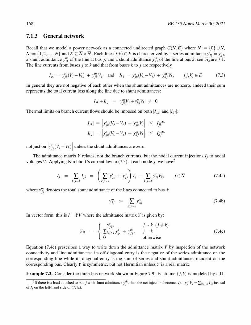
7.1.3 General network

Recall that we model a power network as a connected undirected graph G(N,E) where N := {0} [ N,N := {1,2, . . . ,N} and E ✓ N ⇥ N. Each line ( j,k) 2 E is characterized by a series admittance ys

jk = ysk j,

a shunt admittance ymjk of the line at bus j, and a shunt admittance ym

k j of the line at bus k; see Figure 7.1.The line currents from buses j to k and that from buses k to j are respectively

I jk = ysjk(Vj �Vk) + ym

jk Vj and Ik j = ysjk(Vk �Vj) + ym

k j Vk, ( j,k) 2 E (7.3)

In general they are not negative of each other when the shunt admittances are nonzero. Indeed their sumrepresents the total current loss along the line due to shunt admittances:

I jk + Ik j = ymjkVj + ym

k jVk 6= 0

Thermal limits on branch current flows should be imposed on both |I jk| and |Ik j|:

|I jk| =��ys

jk(Vj �Vk) + ymjk Vj

�� Imaxjk

|Ik j| =��ys

jk(Vk �Vj) + ymk j Vk

�� Imaxk j

not just on��ys

jk(Vj �Vk)�� unless the shunt admittances are zero.

The admittance matrix Y relates, not the branch currents, but the nodal current injections I j to nodalvoltages V . Applying Kirchhoff’s current law to (7.3) at each node j, we have2

I j = Âk: j⇠k

I jk =

Âk: j⇠k

ysjk + ym

j j

!Vj � Â

k: j⇠kys

jkVk, j 2 N (7.4a)

where ymj j denotes the total shunt admittance of the lines connected to bus j:

ymj j := Â

k: j⇠kym

jk (7.4b)

In vector form, this is I = YV where the admittance matrix Y is given by:

Yjk =

8<

:

�ysjk, j ⇠ k ( j 6= k)

Âl: j⇠l ysjl + ym

j j, j = k0 otherwise

(7.4c)

Equation (7.4c) prescribes a way to write down the admittance matrix Y by inspection of the networkconnectivity and line admittances: its off-diagonal entry is the negative of the series admittance on thecorresponding line while its diagonal entry is the sum of series and shunt admittances incident on thecorresponding bus. Clearly Y is symmetric, but not Hermitian unless Y is a real matrix.

Example 7.2. Consider the three-bus network shown in Figure 7.9. Each line ( j,k) is modeled by a P-2If there is a load attached to bus j with shunt admittance ysh

j , then the net injection becomes I j �yshj Vj = Âk: j⇠k I jk instead

of I j on the left-hand side of (7.4a).

EE 135 Notes March 30, 2021 169

V1 V2

I2I1

y12s , y12

m , y21m( )

y13s , y13

m, y31m( )

V3

I3

y23s , y23

m , y32m( )

I12

I13

I21

Figure 7.9: Three-bus network of Example 7.2.

model with a series admittance ysjk and shunt admittances ym

jk and ymk j (not necessarily equal) at two ends

of the line. The sending-end branch current from bus j to bus k is I jk and that from bus k to bus j is Ik j.Applying Kirchhoff’s current law at bus 1 gives

I12 = ys12(V1 �V2) + ym

12V1

I13 = ys13(V1 �V3) + ym

13V1

) I1 = I12 + I13 = (ys12 + ys

13 + ym12 + ym

13)V1 � ys12V2 � ys

13V3

Similarly applying KCL at buses 2 and 3 we obtain2

4I1I2I3

3

5 =

2

4ys

12 + ys13 + ym

11 �ys12 �ys

13�ys

12 ys12 + ys

23 + ym22 �ys

23�ys

13 �ys23 ys

13 + ys23 + ym

33

3

5

| {z }Y

2

4V1V2V3

3

5

where

ysjk = ys

k j and ymj j := Â

k: j⇠kym

jk

Again the off-diagonal entries of the admittance matrix Y are given by the series admittances on the lines:

Yjk :=⇢

�ysjk if j ⇠ k ( j 6= k)0 otherwise

and the diagonal entries of Y by the sum of series and shunt admittances incident on buses j:

Yj j := Âk: j⇠k

ysjk + ym

j j

170 EE 135 Notes March 30, 2021

The admittance matrix can also be expressed in terms of more elementary matrices. This represen-tation is useful for constructing the admittance matrix that models the end-to-end behavior of a systemconsisting of a cascade of subsystems, e.g., in modeling the external behavior of an unbalanced three-phase transformer. Fix an arbitrary orientation for the graph G(N,E) so that a line l = i ! j 2 E is nowconsidered pointing from bus i to bus j. Let C 2 {�1,0,1}(N+1)⇥M be the bus-by-line incidence matrixdefined by:

C jl =

8<

:

1 if l = j ! k for some bus k�1 if l = i ! j for some bus i0 otherwise

Let Y s := diag(ysl l 2 E) be the |E|⇥ |E| diagonal matrix with the series admittances ys

l as its diagonal en-tries. Let Y m := diag(ym

j j, j 2 N) be the (N +1)⇥ (N +1) diagonal matrix with the total shunt admittancesym

j j in (7.4b) as its diagonal entries. Then the admittance matrix (7.4c) is:

Y = CY sCT+ Y m

Clearly the matrix CY sCT has zero row and column sums.

7.1.4 Kron reduction

In many applications we are interested in the relation between the current injections and voltages at onlya subset Nred ⇢ N of the buses. For example we are interested in the external behavior of a system definedby the relationship between currents and voltages at only terminal buses. Denote the number of buses inNred also by Nred. Without loss of generality we can partition the buses such that I1 2 C

Nred denotes thefirst Nred current injections and I2 the remaining N + 1 � Nred current injections. Similarly partition thevoltages into (V1,V2) with V1 2 C

Nred , V2 2 CN+1�Nred . Partition the admittance matrix Y so that

I1I2

�=

Y11 Y12Y21 Y22

�

| {z }Y

V1V2

�

If Y22 is invertible then we can eliminate V2 by substituting V2 = �Y �122 Y21V1 +Y �1

22 I2 to obtain�Y11 �Y12Y �1

22 Y21�

V1 = I1 � Y12Y �122 I2 (7.5)

The Nred ⇥ Nred matrix Y/Y22 := Y11 �Y12Y �122 Y21 is called the Schur complement of Y22 of matrix Y (see

Appendix 26.1.1 for its properties). Since Y is complex symmetric, the Schur complement Y/Y22 is alsocomplex symmetric and hence can be interpreted as the admittance matrix of a reduced network consistingonly of buses in n. It describes the effective connectivity and line admittances of the reduced network andI1 �Y12Y �1

22 I2 describes the effective current injections at these buses. This is called a Kron reduction ofnetwork G.

Given current injections I = (I1, I2), we can obtain V1 in terms of the Schur complement Y/Y22 and theeffective current injections:

V1 =�Y11 �Y12Y �1

22 Y21��1 �I1 � Y12Y �1

22 I2�

EE 135 Notes March 30, 2021 171

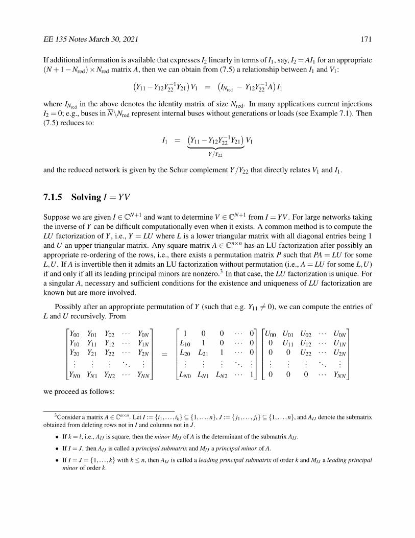
If additional information is available that expresses I2 linearly in terms of I1, say, I2 = AI1 for an appropriate(N +1�Nred)⇥Nred matrix A, then we can obtain from (7.5) a relationship between I1 and V1:

�Y11 �Y12Y �1

22 Y21�

V1 =�INred � Y12Y �1

22 A�

I1

where INred in the above denotes the identity matrix of size Nred. In many applications current injectionsI2 = 0; e.g., buses in N\Nred represent internal buses without generations or loads (see Example 7.1). Then(7.5) reduces to:

I1 =�Y11 �Y12Y �1

22 Y21�

| {z }Y/Y22

V1

and the reduced network is given by the Schur complement Y/Y22 that directly relates V1 and I1.

7.1.5 Solving I = YV

Suppose we are given I 2 CN+1 and want to determine V 2 C

N+1 from I = YV . For large networks takingthe inverse of Y can be difficult computationally even when it exists. A common method is to compute theLU factorization of Y , i.e., Y = LU where L is a lower triangular matrix with all diagonal entries being 1and U an upper triangular matrix. Any square matrix A 2 C

n⇥n has an LU factorization after possibly anappropriate re-ordering of the rows, i.e., there exists a permutation matrix P such that PA = LU for someL,U . If A is invertible then it admits an LU factorization without permutation (i.e., A = LU for some L,U)if and only if all its leading principal minors are nonzero.3 In that case, the LU factorization is unique. Fora singular A, necessary and sufficient conditions for the existence and uniqueness of LU factorization areknown but are more involved.

Possibly after an appropriate permutation of Y (such that e.g. Y11 6= 0), we can compute the entries ofL and U recursively. From

2

666664

Y00 Y01 Y02 · · · Y0NY10 Y11 Y12 · · · Y1NY20 Y21 Y22 · · · Y2N

......

... . . . ...YN0 YN1 YN2 · · · YNN

3

777775=

2

666664

1 0 0 · · · 0L10 1 0 · · · 0L20 L21 1 · · · 0

......

... . . . ...LN0 LN1 LN2 · · · 1

3

777775

2

666664

U00 U01 U02 · · · U0N0 U11 U12 · · · U1N0 0 U22 · · · U2N...

...... . . . ...

0 0 0 · · · YNN

3

777775

we proceed as follows:

3Consider a matrix A 2 Cn⇥n. Let I := {i1, . . . , ik} ✓ {1, . . . ,n}, J := { j1, . . . , jl} ✓ {1, . . . ,n}, and AIJ denote the submatrix

obtained from deleting rows not in I and columns not in J.

• If k = l, i.e., AIJ is square, then the minor MIJ of A is the determinant of the submatrix AIJ .

• If I = J, then AIJ is called a principal submatrix and MIJ a principal minor of A.

• If I = J = {1, . . . ,k} with k n, then AIJ is called a leading principal submatrix of order k and MIJ a leading principalminor of order k.

172 EE 135 Notes March 30, 2021

1. The 0th row of U is set to the 0th row of Y since L00 = 1:

U0 j = Y0 j, j = 0, . . . ,N

2. To compute row-1 entry L10 of L, we have

Y10 = L10U00 ) L10 =Y10

U00

To compute row-1 entries U1 j of U , we have for columns j = 1, . . . ,N,

Y1 j = L10U0 j +U1 j ) U1 j = Y1 j �L10U0 j

3. In general, to compute row-i entries Li j of L (i = 2, . . . ,N), we have for columns j = 0, . . . , i�1,

Yi0 = Li0U00 ) Li0 =Yi0

U00

Yi1 = Li0U01 +Li1U11 ) Li1 =1

U11(Yi1 �Li0U01)

......

Yi(i�1) =i�2

Âj=0

Li jUj(i�1) +Li(i�1)U(i�1)(i�1) ) Li(i�1) =1

U(i�1)(i�1)

Yi(i�1) �

i�2

Âj=0

Li jUj(i�1)

!

To compute row-i entries Ui j of U (i = 2, . . . ,N), we have for columns j = i, . . . ,N,

Yii =i�1

Âj=0

Li jUji +Uii ) Uii = Yii �i�1

Âj=0

Li jUji

Yi(i+1) =i�1

Âj=0

Li jUj(i+1) +Ui(i+1) ) Ui(i+1) = Yi(i+1) �i�1

Âj=0

Li jUj(i+1)

......

YiN =i�1

Âj=0

Li jUjN +UiN ) UiN = YiN �i�1

Âj=0

Li jUjN

Once the factorization is obtained we have I = YV = LUV . Hence, given I, V can be solved in twosteps from:

I = LV (7.6)V = UV (7.7)

In step 1, V is solved using (7.6) by forward substitution (compute V1 then V2 and so on). In step 2, V issolved using (7.7) by backward substitution (compute Vn then Vn�1 and so on).

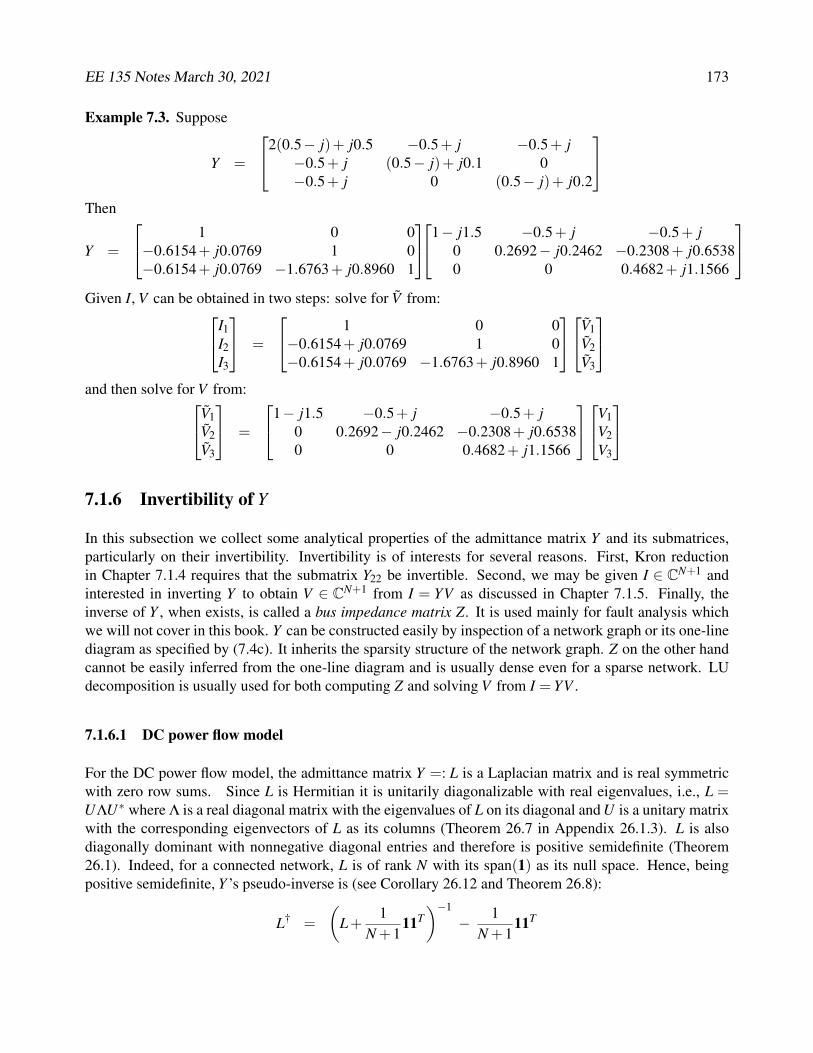
EE 135 Notes March 30, 2021 173

Example 7.3. Suppose

Y =

2

42(0.5� j)+ j0.5 �0.5+ j �0.5+ j

�0.5+ j (0.5� j)+ j0.1 0�0.5+ j 0 (0.5� j)+ j0.2

3

5

Then

Y =

2

41 0 0

�0.6154+ j0.0769 1 0�0.6154+ j0.0769 �1.6763+ j0.8960 1

3

5

2

41� j1.5 �0.5+ j �0.5+ j

0 0.2692� j0.2462 �0.2308+ j0.65380 0 0.4682+ j1.1566

3

5

Given I, V can be obtained in two steps: solve for V from:2

4I1I2I3

3

5 =

2

41 0 0

�0.6154+ j0.0769 1 0�0.6154+ j0.0769 �1.6763+ j0.8960 1

3

5

2

4V1V2V3

3

5

and then solve for V from:2

4V1V2V3

3

5 =

2

41� j1.5 �0.5+ j �0.5+ j

0 0.2692� j0.2462 �0.2308+ j0.65380 0 0.4682+ j1.1566

3

5

2

4V1V2V3

3

5

7.1.6 Invertibility of Y

In this subsection we collect some analytical properties of the admittance matrix Y and its submatrices,particularly on their invertibility. Invertibility is of interests for several reasons. First, Kron reductionin Chapter 7.1.4 requires that the submatrix Y22 be invertible. Second, we may be given I 2 C

N+1 andinterested in inverting Y to obtain V 2 C

N+1 from I = YV as discussed in Chapter 7.1.5. Finally, theinverse of Y , when exists, is called a bus impedance matrix Z. It is used mainly for fault analysis whichwe will not cover in this book. Y can be constructed easily by inspection of a network graph or its one-linediagram as specified by (7.4c). It inherits the sparsity structure of the network graph. Z on the other handcannot be easily inferred from the one-line diagram and is usually dense even for a sparse network. LUdecomposition is usually used for both computing Z and solving V from I = YV .

7.1.6.1 DC power flow model

For the DC power flow model, the admittance matrix Y =: L is a Laplacian matrix and is real symmetricwith zero row sums. Since L is Hermitian it is unitarily diagonalizable with real eigenvalues, i.e., L =ULU⇤ where L is a real diagonal matrix with the eigenvalues of L on its diagonal and U is a unitary matrixwith the corresponding eigenvectors of L as its columns (Theorem 26.7 in Appendix 26.1.3). L is alsodiagonally dominant with nonnegative diagonal entries and therefore is positive semidefinite (Theorem26.1). Indeed, for a connected network, L is of rank N with its span(1) as its null space. Hence, beingpositive semidefinite, Y ’s pseudo-inverse is (see Corollary 26.12 and Theorem 26.8):

L† =

✓L+

1N +1

11T◆�1

� 1N +1

11T

174 EE 135 Notes March 30, 2021

Since the network is connected, any strict principal submatrix Y22 of Y is strictly diagonally dominant, andhence is positive definite and invertible (Theorem 26.1).s

7.1.6.2 General power flow models.

We now turn to the invertibility of Y and its principal submatrices in general power flow models. We firstconsider the case where the line shunts are negligible, i.e., ym

j j = 0 for all j 2 N, so that all row sums ofY are zero. In this case Y is not invertible and we present its pseudo-inverse. We then discuss conditionsunder which Y and its principal submatrix Y22 are invertible.

Pseudo-inverse of Y . When ymj j = 0 for all j 2 N, the (N + 1) ⇥ (N + 1) matrix Y has rank N for a

connected network and its null space is span(1) (Exercise 7.2). We can obtain its pseudo-inverse throughdiagonalization. Since Y is complex symmetric but not Hermitian in general, it may no longer be unitarilydiagonalizable. A matrix is unitarily diagonalizable if and only if it is normal (Theorem 26.6 in Appendix26.1.3). Y may or may not be normal. See Exercise 7.1 for sufficient conditions under which Y is normaland hence unitarily diagonalizable. When Y is not normal, it can still be factorized using singular valuedecomposition, according to Theorem 26.9 in Appendix 26.1.3.

Theorem 7.1 (Factorization of Y ). There exists a unitary matrix W 2 C(N+1)⇥(N+1) and a real nonnegative

diagonal matrix S :=diag(s1, . . . ,sN+1) such that Y = WSW T where

1. the diagonal entries of S are the nonnegative square roots of the eigenvalues of YY ;

2. the columns of W are the corresponding orthonormal set of eigenvectors of YY .

The singular value decomposition in Theorem 7.1 implies that the pseudo-inverse of Y is (see Appendix26.1.4)

Y † := WS†W ⇤ (7.8)

where S† is the real diagonal matrix of rank N obtained from S by replacing the nonzero singular valuessi by 1/si, and taking the transpose.

For each current vector I with 1T I = 0 there is a subspace of solutions to I = YV given by

V = Y †I + b1, b 2 C

parametrized by b . Hence V is unique up to an arbitrary reference voltage. For example the solutionV = Y †I corresponds to a solution with b = 0. Alternatively b can be chosen so that V0 = 1\0� at theslack bus 0.

Inverse of Y . When there are nonzero shunt elements with appropriate signs, Y is invertible. Unlike theLaplacian matrix Y = L in the DC power flow model, a general admittance matrix Y may not be diagonallydominant, i.e., |Yii| � Â j: j 6=i |Yi j| may not hold for all i. This can be the case for a transmission line since

EE 135 Notes March 30, 2021 175

the susceptances of line shunts and those of series admittances are typically of different signs; see Remark7.1.

To derive conditions that guarantee the invertibility of Y , recall that Y is not invertible if and only ifzero is an eigenvalue of Y . If l is an eigenvalue and a 2 C

N+1 is a corresponding eigenvector then

aHY a = ÂjÂk

Yjka⇤j ak = l ||a||2 (7.9)

where || · || denotes the Euclidean norm. Hence for Y to be invertible it is sufficient, but not necessary, thataHY a 6= 0 for all nonzero vectors a 2 C

N+1 (see Exercise 7.4). Substituting (7.4c) into (7.9) we have

aHY a = Âj

Âk:k⇠ j

ysjk + ym

j j

!|a j|2 � Â

k:k⇠ jys

jk a⇤j ak

!

= Â( j,k)2E

ysjk�|a j|2 �a⇤

j ak �a ja⇤k + |ak|2

�+ Â

j2Nym

j j |a j|2

= Â( j,k)2E

ysjk��a j �ak

��2 + Âj2N

ymj j |a j|2

where we have used ysjk = ys

k j in the second equality. Let

ysjk =: gs

jk � ibsjk and ym

j j =: gmj j � ibm

j j

Then

aHY a =

0

@ Â( j,k)2E

gsjk��a j �ak

��2 + Âj2N

gmj j |a j|2

1

A� i

0

@ Â( j,k)2E

bsjk��a j �ak

��2 + Âj2N

bmj j |a j|2

1

A(7.10)

Previous discussion implies that, for Y to be invertible, it is necessary to have at least one nonzeroshunt element. Additional conditions are needed to guarantee invertibility, as follows:

C7.1: There is at least one bus j 2 N where ymj j 6= 0. All nonzero gm

j j have the same sign and allnonzero bm

j j have the same sign.

C7.2: All nonzero gsjk have the same sign and all nonzero bs

jk have the same sign.

C7.3a: For all lines ( j,k) 2 E, gsjk 6= 0. If gm

j j 6= 0 then it has the same sign as all nonzero gsjk.

C7.3b: For all lines ( j,k) 2 E, bsjk 6= 0. If bm

j j 6= 0 then it has the same sign as all nonzero bsjk.

C7.3c: If gmj j 6= 0 then it has the same sign as all nonzero gs

jk, and if bmj j 6= 0 then it has the same sign

as all nonzero bsjk.

Conditions C7.3a, C7.3b, C7.3c are not mutually exclusive. These conditions imply the invertibility of Y .

Theorem 7.2. Suppose the network is connected and conditions C7.1, C7.2, and one of C7.3a, C7.3b,C7.3c hold. Then Y �1 exists.

176 EE 135 Notes March 30, 2021

Proof. Suppose conditions C7.2, C7.1 and C7.3a hold but there exists a nonzero a 2 CN+1 such that

aHY a = 0. Then C7.2 and C7.3a imply that, for the real part of (7.10) to be zero, we must have a j = akfor all ( j,k) 2 E since the network is connected. This means that

aHY a =

0

@Âj2N

gmj j � i Â

j2Nbm

j j

1

A |a j|2 = Âj2N

ymj j |a j|2

C7.1 implies that there is at least one bus i 2 N with nonzero ymii . Hence aHY a = 0 implies ai = 0. Since

a j = ak for all ( j,k) 2 E and the network is connected, a j = ai = 0 for all j 2 N, contradicting that a isa nonzero vector. Hence C7.2, C7.1 and C7.3a imply that aHY a 6= 0 for all nonzero a 2 C

N+1, and Y �1

exists.

If condition C7.3a is replaced by C7.3b, the argument is symmetric. Suppose neither C7.3a nor C7.3bholds, i.e., there are lines ( j,k) 2 E where gs

jk = 0 and bsjk 6= 0 and there are lines ( j,k) 2 E where gs

jk 6= 0and bs

jk = 0, but C7.3c holds. Since for every line ( j,k) 2 E either gsjk 6= 0 or bs

jk 6= 0, C7.2 and C7.3c implythat a j = ak (from (7.10)). C7.1 then implies that there is a bus i where either gm

ii 6= 0 or bmii 6= 0, implying

that ai = 0. The connectedness of the graph again implies that a j = ai = 0 for all j 2 N, contradictingthat a is a nonzero vector. This completes the proof.

For transmission line models, the conditions in Theorem 7.2 are usually satisfied.

Remark 7.1 (Transmission line). 1. A transmission line ( j,k) typically has nonnegative series con-ductance gs

jk � 0 and positive series susceptance bsjk > 0 (inductive line). Its shunt conductance

gmjk � 0 is usually nonnegative, but shunt susceptance bm

jk 0 is usually nonpositive (capacitive),so that usually gm

j j := Âk⇠ j gmjk � 0 and bm

j j := Âk⇠ j bmjk 0. Hence conditions C7.1 and C7.2 are

usually satisfied. If all lines have nonzero resistance, i.e., gsjk > 0 for all ( j,k) 2 E, then condition

C7.3a is satisfied.

2. Since bsjk > 0 but bm

jk 0 for a typical transmission line, Condition C7.3b and C7.3c are not usuallysatisfied.

The conditions in Theorem 7.2 are sufficient but not necessary, as the next example shows.

Example 7.4 (Transformer connected to a transmission line). Consider the model in Figure 7.7 of a non-ideal off-nominal transformer connected to a transmission line in Example 7.1 with corresponding admit-tance matrix Y given by (7.2). The parameters of lines (1,3) and (2,3) are

(ys13,y

m13,y

m31) :=

⇣yl,0,ym

⌘

(ys23,y

m23,y

m32) := (ny,(1�n)y,n(n�1)y)

where n is the turns ratio of the transformer. The series admittance y of the line and the series and shuntadmittances (yl,ym) of the transformer are of the form:

y = gs � ibs, yl =1

r + jwLl = gl � ibl, ym =1

jwLm = �ibm

EE 135 Notes March 30, 2021 177

with gs,bs,gl,bljk,b

mjk � 0. Hence

ys13 = ys

31 = gl � ibl, ys23 = ys

32 = ngs � inbs

ym11 = 0, ym

22 = (1�n)gs � i(1�n)bs, ym33 = n(n�1)gs � i(n(n�1)bs +bm)

Condition C1 is satisfied but C2 is not since gm22 := (1 � n)gs and gm

33 := n(n � 1)gs have opposite signsunless n = 1. Using (7.10), however, we have

Re�aHY a

�=

⇣gl|a1 �a3|2 +ngs|a2 �a3|2

⌘+�(1�n)gs|a2|2 +n(n�1)gs|a3|2

�

= gl|a1 �a3|2 + gs|a2 �na3|2

and hence

Re�aHY a

�= 0 if and only if a1 = a3 =

a2

n(7.11)

On the other hand

�Im�aHY a

�=

⇣bl|a1 �a3|2 +nbs|a2 �a3|2

⌘+�(1�n)bs|a2|2 +(n(n�1)bs +bm) |a3|2

�

= bl|a1 �a3|2 + bs|a2 �na3|2 + bm|a3|2

In light of (7.11), if bm > 0 then aHY a = 0 if and only if a1 = a2 = a3 = 0. Hence if bm > 0 then Y isinvertible.

On the other hand, if bm = 0 then there exists nonzero a 2 C3 with aHY a = 0. Exercise 7.4 says that,

since Y is complex symmetric (but not Hermitian), this does not necessarily imply Y a = 0 and hence maynot imply that Y is singular. Using the admittance matrix (given in (7.2))

Y =

2

4yl 0 �yl

0 y �ny�yl �ny yl + ym +n2y

3

5

it can be verified that, when ym = �ibm = 0, a :=⇥1 n 1

⇤T is indeed an eigenvector of Y correspondingto zero eigenvalue. Hence Y is singular if the (only) shunt element bm in the model of Example 7.1 is zero,even when ym

22 and ym33, which originate from the effect of an ideal transformer, are nonzero.

7.1.6.3 Invertibility of Y22 in Kron reduction

Unlike the Laplacian matrix Y = L in the DC power flow model, a principal submatrix Y22 may not bestrictly diagonally dominant, i.e., |Yii| > Â j: j 6=i |Yi j| may not hold for all i. We now derive sufficientconditions for its invertibility.

To simplify notation let n := N + 1 � Nred be the dimension of the square matrix Y22 and suppose0 < n < N + 1. For the rest of this subsection denote the ( j,k) entry of a matrix A by A[ j,k], e.g.,Y [ j,k],Y22[ j,k]. Note that the indices j,k run from Nred +1, . . . ,N +1, not 1, . . . ,n. The argument is similar

178 EE 135 Notes March 30, 2021

to that for the invertibility of Y . By definition Y22 is not invertible if and only if zero is an eigenvalue ofY22. If l is an eigenvalue and a 2 C

n is a corresponding eigenvector then

aHY22a =N+1

Âj=Nred+1

N+1

Âk=Nred+1

Y [ j,k]a⇤j ak = l ||a||2 (7.12)

where || · || denotes the Euclidean norm. Hence for Y22 to be invertible it is sufficient, but not necessary,that aHY22a 6= 0 for all nonzero vectors a 2 C

n (see Exercise 7.4). We have from (7.4c)

Y22[ j, j] = ÂkNred:k⇠ j

ysjk + Â

k>Nred:k⇠ jys

jk + ymj j, j = Nred +1, . . . ,N +1

Substituting this and Y [ j,k] = �ysjk for j ⇠ k into (7.12) we have

aHY22a = Âj>Nred

ÂkNred:k⇠ j

ysjk + Â

k>Nred:k⇠ jys

jk + ymj j

!|a j|2 � Â

k>Nred:k⇠ jys

jk a⇤j ak

!

= Âj,k>Nred: j⇠k

ysjk�|a j|2 �a⇤

j ak �a ja⇤k + |ak|2

�+ Â

j>Nred

ÂkNred:k⇠ j

ysjk + ym

j j

!|a j|2

= Âj,k>Nred: j⇠k

ysjk��a j �ak

��2 + Âj>Nred

ÂkNred:k⇠ j

ysjk + ym

j j

!|a j|2

where we have used ysjk = ys

k j in the second equality. The first term sums over links in the subgraphinduced by N \Nred. The second term sums over links between the subgraph induced by N \Nred and thatby Nred. Recall ys

jk =: gsjk � ibs

jk and ymj j =: gm

j j � ibmj j. Then

Re�aHY22a

�= Â

j,k>Nred: j⇠kgs

jk��a j �ak

��2 + Âj>Nred

ÂkNred:k⇠ j

gsjk + gm

j j

!|a j|2 (7.13a)

�Im�aHY22a

�= Â

j,k>Nred: j⇠kbs

jk��a j �ak

��2 + Âj>Nred

ÂkNred:k⇠ j

bsjk + bm

j j

!|a j|2 (7.13b)

Consider

C7.4: There is at least one bus j > Nred with ÂkNred:k⇠ j ysjk + ym

j j 6= 0.

C7.5a: For all lines j,k > Nred, j ⇠ k, gsjk are nonzero and have the same sign. If for any j > Nred,

ÂkNred:k⇠ j

gsjk + gm

j j 6= 0

then it has the same sign as gsjk for j,k > Nred, j ⇠ k.

C7.5b: For all lines j,k > Nred, j ⇠ k, bsjk are nonzero and have the same sign. If for any j > Nred,

ÂkNred:k⇠ j

bsjk + bm

j j 6= 0

then it has the same sign as bsjk for j,k > Nred, j ⇠ k.

EE 135 Notes March 30, 2021 179

Conditions C7.5a and C7.5b are not mutually exclusive. They imply the invertibility of Y22 and hence thevalidity of the Kron reduction.

Theorem 7.3. Suppose the network is connected and C7.4 and one of C7.5a or C7.5b hold. Then Y �122

exists.

Proof. Suppose for the sake of contradiction that conditions C7.4 and C7.5a hold but there exists a nonzeroa 2 C

n such that aHY22a = 0. Then from (7.13a), Re(aHY22a) = 0 implies that, under conditions C7.4and C7.5a,

a j = ak, j,k = Nred +1, . . . ,N +1 (7.14)

since the graph is connected. Then (7.13) implies that

aHY22a = Âj>Nred

�G j � iB j

�|a j|2 = |aN+1|2 Â

j>Nred

�G j � iB j

�

where

G j := ÂkNred:k⇠ j

gsjk + gm

j j and B j := ÂkNred:k⇠ j

bsjk + bm

j j, j = Nred +1, . . . ,N +1

Condition C7.4 implies that Â j>Nred G j 6= 0. Hence Re(aHY22a) = 0 only if aN+1 = 0. From (7.14) wetherefore have a j = aN+1 = 0 for all j > Nred, contradicting that a is a nonzero vector. Hence Y �1

22 exists.

If condition C7.5b instead of C7.5a holds, the argument is symmetric. This completes the proof.

Remark 7.2 (Transmission line). As discussed in Remark 7.1, for a transmission line, we usually havegs

jk � 0, bsjk > 0, gm

j j � 0 and bmj j 0. If all lines ( j,k), j,k > Nred, have nonzero resistance, then condition

C7.5a is satisfied. For C7.5b, even though bsjk and bm

j j have opposite signs, the shunt susceptances bmjk

are typically much smaller than the series susceptances bsjk such that usually ÂkNred:k⇠ j bs

jk + bmj j � 0,

i.e., it has the same sign as bsjk. Hence C7.5b is likely to be satisfied since bs

jk are usually nonzero fortransmission lines. Finally condition C7.4 involves lines between the bus j > Nred with zero injection andother buses k Nred with possibly nonzero injections. It requires that the sum of series admittances ys

jk onthese lines is not canceled out by the total shunt admittance ym

j j at bus j. This is usually satisfied since ymjk

are much smaller in magnitude than ysjk. For example, for transmission lines of medium length we often

assume gmj j = 0.

7.1.7 Summary

In summary we have explained how to model different network components, such as transmission lines,transformers, generators and loads, as nodes in a graph with links connecting these nodes parameterizedby (ys

jk,ymjk,y

mk j). This can be described by an admittance matrix Y . The equation I = YV relates current

injections to voltages in the network. Finally we have discussed sufficient conditions for the invertibilityof Y and its principal submatrices.

In this setting if all generators and loads can be modeled by constant current sources then, given I, thevoltages V on the network can be computed from the equation I = YV as discussed in Chapter 7.1.5. This

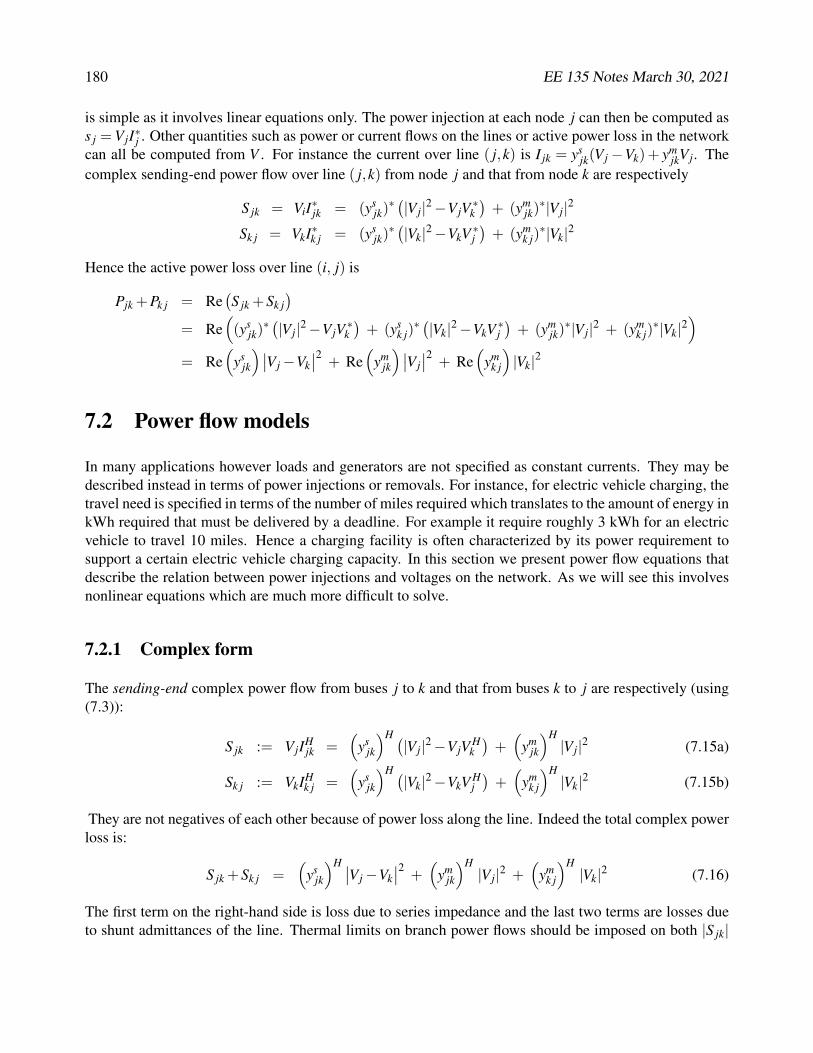
180 EE 135 Notes March 30, 2021

is simple as it involves linear equations only. The power injection at each node j can then be computed ass j = VjI⇤

j . Other quantities such as power or current flows on the lines or active power loss in the networkcan all be computed from V . For instance the current over line ( j,k) is I jk = ys

jk(Vj �Vk)+ ymjkVj. The

complex sending-end power flow over line ( j,k) from node j and that from node k are respectively

S jk = ViI⇤jk = (ys

jk)⇤ �|Vj|2 �VjV ⇤

k�

+ (ymjk)

⇤|Vj|2

Sk j = VkI⇤k j = (ys

jk)⇤ �|Vk|2 �VkV ⇤

j�

+ (ymk j)

⇤|Vk|2

Hence the active power loss over line (i, j) is

Pjk +Pk j = Re�S jk +Sk j

�

= Re⇣(ys

jk)⇤ �|Vj|2 �VjV ⇤

k�

+ (ysk j)

⇤ �|Vk|2 �VkV ⇤j�

+ (ymjk)

⇤|Vj|2 + (ymk j)

⇤|Vk|2⌘

= Re⇣

ysjk

⌘��Vj �Vk��2 + Re

⇣ym

jk

⌘��Vj��2 + Re

⇣ym

k j

⌘|Vk|2

7.2 Power flow models

In many applications however loads and generators are not specified as constant currents. They may bedescribed instead in terms of power injections or removals. For instance, for electric vehicle charging, thetravel need is specified in terms of the number of miles required which translates to the amount of energy inkWh required that must be delivered by a deadline. For example it require roughly 3 kWh for an electricvehicle to travel 10 miles. Hence a charging facility is often characterized by its power requirement tosupport a certain electric vehicle charging capacity. In this section we present power flow equations thatdescribe the relation between power injections and voltages on the network. As we will see this involvesnonlinear equations which are much more difficult to solve.

7.2.1 Complex form

The sending-end complex power flow from buses j to k and that from buses k to j are respectively (using(7.3)):

S jk := VjIHjk =

⇣ys

jk

⌘H �|Vj|2 �VjV H

k�

+⇣

ymjk

⌘H|Vj|2 (7.15a)

Sk j := VkIHk j =

⇣ys

jk

⌘H �|Vk|2 �VkV H

j�

+⇣

ymk j

⌘H|Vk|2 (7.15b)

They are not negatives of each other because of power loss along the line. Indeed the total complex powerloss is:

S jk +Sk j =⇣

ysjk

⌘H ��Vj �Vk��2 +

⇣ym

jk

⌘H|Vj|2 +

⇣ym

k j

⌘H|Vk|2 (7.16)

The first term on the right-hand side is loss due to series impedance and the last two terms are losses dueto shunt admittances of the line. Thermal limits on branch power flows should be imposed on both |S jk|

EE 135 Notes March 30, 2021 181

and |Sk j|:

|S jk| =

��⇣

ysjk


k�

+⇣

ymjk

⌘H|Vj|2

�� Smaxjk

|Sk j| =

��⇣

ysjk

⌘H �|Vk|2 �VkV H

j�

+⇣

ymk j

⌘H|Vk|2

�� Smaxk j

not just on��⇣

ysjk


k�� and

��⇣

ysjk

⌘H ⇣|Vk|2 �VkV H

j

⌘�� unless the shunt admittances are zero.

If the shunt admittances of the line ymjk and ym

k j are zero then the power loss has a simple relation withline current I jk = �Ik j. Setting ym

jk = ymk j = 0 in (7.16) and (7.3) we have

S jk +Sk j = zsjk ·��ys

jk

��2 ��Vj �Vk

��2 = zsjk��I jk��2

because I jk = ysjk(Vj �Vk) = �Ik j when the shunt elements are zero. This is not the case otherwise.

The bus injection model (BIM) in its complex form is defined by power balance s j = Âk: j⇠k S jk at eachnode j. This leads to the power flow equations that relate power injections and voltages through (7.15):

s j = Âk: j⇠k

⇣ys

jk


k�

+�ym

j j�H |Vj|2, j 2 N (7.17a)

where, from (7.4b), the total shunt admittance ymj j := Âk: j⇠k ym

jk associated with bus j is the sum of shuntadmittances ym

jk of all lines ( j,k) incident on bus j. We can also express (7.17a) in terms of the elementsof the admittance matrix Y as

s j =N

Âk=0

Y Hjk VjV H

k , j 2 N (7.17b)

where Y is given by:

Yjk =

8><

>:

�⇣

ysjk

⌘, j ⇠ k ( j 6= k)

Âi: j⇠i ysji + ym

j j j = k0 otherwise

When the total shunt admittance ymj j = 0, (7.17a) reduces to

s j = Âk: j⇠k

⇣ys

jk


k�, j 2 N

For convenience we include V0 in the vector variable V := (Vj, j 2 N) with the understanding that V0 :=1\0� is fixed. There are N +1 equations in (7.17a) in 2(N +1) complex variables (s j,Vj, j 2 N).

182 EE 135 Notes March 30, 2021

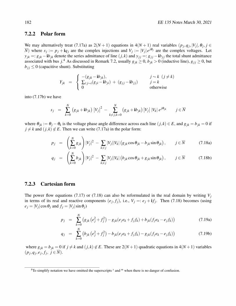
7.2.2 Polar form

We may alternatively treat (7.17a) as 2(N + 1) equations in 4(N + 1) real variables (p j,q j, |Vj|,q j, j 2N) where s j := p j + iq j are the complex injections and Vj := |Vj|e jq j are the complex voltages. Lety jk =: g jk � ib jk denote the series admittance of line ( j,k) and y j j =: g j j � ib j j the total shunt admittanceassociated with bus j.4 As discussed in Remark 7.2, usually g jk � 0, b jk > 0 (inductive line), g j j � 0, butb j j 0 (capacitive shunt). Substituting

Yjk =

8<

:

�(g jk � ib jk), j ⇠ k ( j 6= k)Âi: j⇠i(g ji � ib ji) + (g j j � ib j j) j = k0 otherwise

into (7.17b) we have

s j =N

Âk=0

�g jk + ib jk

� ��Vj��2 �

N

Âk 6= j,k=0

�g jk + ib jk

��Vj�� |Vk| e jq jk j 2 N

where q jk := q j �qk is the voltage phase angle difference across each line ( j,k) 2 E, and g jk = b jk = 0 ifj 6= k and ( j,k) 62 E. Then we can write (7.17a) in the polar form:

p j =

N

Âk=0

g jk

!|Vj|2 � Â

k 6= j|Vj||Vk|

�g jk cosq jk �b jk sinq jk

�, j 2 N (7.18a)

q j =

N

Âk=0

b jk

!|Vj|2 � Â

k 6= j|Vj||Vk|

�b jk cosq jk +g jk sinq jk

�, j 2 N (7.18b)

7.2.3 Cartesian form

The power flow equations (7.17) or (7.18) can also be reformulated in the real domain by writing Vjin terms of its real and reactive components (e j, f j), i.e., Vj =: e j + i f j. Then (7.18) becomes (usinge j = |Vj|cosq j and f j = |Vj|sinq j)

p j =N

Âk=0

�g jk�e2

j + f 2j��g jk(e jek + f j fk)+b jk( f jek � e j fk)

�(7.19a)

q j =N

Âk=0

�b jk�e2

j + f 2j��b jk(e jek + f j fk)�g jk( f jek � e j fk)

�(7.19b)

where g jk = b jk = 0 if j 6= k and ( j,k) 62 E. These are 2(N +1) quadratic equations in 4(N +1) variables(p j,q j,e j, f j, j 2 N).

4To simplify notation we have omitted the superscripts s and m when there is no danger of confusion.

Chapter 8

Branch flow models

In this chapter we introduce several forms of branch flow models. Whereas a bus injection model consistsof only nodal variables (power and current injections and voltages), a branch flow model involves alsobranch power flows and branch currents. We will present branch flow models in complex form, real form,for general networks and radial networks, with and without line shunts. Finally we present a linearizedmodel for radial networks.

Branch flow models were originally proposed for analyzing radial networks and have been extendedto general networks with cycles. To connect them to the bus injection models we will start with generalnetworks and then specialize to radial networks.

8.1 General network

As in Chapter 7 we model a power network with N + 1 buses and M lines as a connected undirectedgraph G = (N,E) where N := {0}[ N, N := {1,2, . . . ,N} and E ✓ N ⇥ N. A line ( j,k) 2 E, or j ⇠ k, isrepresented by a P-equivalent circuit (ys

jk,ymjk,y

mk j) where ys

jk = ysk j is the series admittance of the line, ym

jkis the shunt admittance of the line at bus j, and ym

k j is the shunt admittance of the line at bus k. Again ymjk

and ymk j are generally unequal.

Complex form. For each bus j 2 N, let s j denote its complex power injection and Vj its voltage phasor.For each line ( j,k) 2 E, let (S jk,Sk j) denote the sending-end branch power flows and (I jk, Ik j,( j,k)) denotethe sending-end branch currents. Let s := (s j, j 2 N), V := (Vj, j 2 N), S := (S jk,Sk j,( j,k) 2 E), andI := (I jk, Ik j,( j,k) 2 E).

The branch flow model (BFM) in the complex form is defined by the following power flow equations

201

202 EE 135 Notes March 30, 2021

in the variables (s,V, I,S) 2 C2(N+1)+4M (from (7.3)(7.15)):

s j = Âk: j⇠k

S jk, j 2 N (8.1a)

S jk = Vj IHjk, Sk j = Vk IH

k j, ( j,k) 2 E (8.1b)I jk = ys

jk(Vj �Vk) + ymjkVj, ( j,k) 2 E (8.1c)

Ik j = ysk j(Vk �Vj) + ym

k jVk, ( j,k) 2 E (8.1d)

where (8.1a) imposes power balance at each bus, (8.1b) defines branch power in terms of the associatedvoltage and current, and (8.1c)(8.1d) describes the Kirchhoff’s laws. For convenience we include V0 in thevector variable V := (Vj, j 2 N) with the understanding that V0 := 1\0� is fixed.

Real form. A branch flow model, called the DistFlow equations, is proposed in [17, 18] for radialnetworks. Its key feature is that it does not involve phase angles of voltage and current phasors. For eachbus j let

• si := (pi,qi) and si := (pi + iqi) represent the real and reactive power injections at bus j;1

• vi represent the squared voltage magnitude at bus j.

For each line ( j,k) let

• S jk = (Pjk,Q jk) and S jk = Pjk + iQ jk represent the sending-end real and reactive branch power flowfrom bus j to bus k, and Sk j represent the sending-end power from k to j;

• ` jk represent the squared current magnitude of the sending-end current from bus j to bus k, and `k jrepresent the squared current magnitude from k to j.

The variables v := (v j, j 2 N) and ` := (` jk,`k j,( j,k) 2 E) will replace the phasors V and I in the model(8.1). The power flow equations below therefore are in terms of a real vector x := (s,v,`,S) 2 R

3(N+1)+4M

that does not involve voltage and phase angles as variables.

The angle information is however embedded in x. Specifically, define for each ( j,k) 2 E

zsjk :=

⇣ys

jk

⌘�1=: zs

k j

a jk := 1+ zsjk ym

jk, ak j := 1+ zsk j ym

k j

Note that a jk = ak j if and only if ymjk = ym

k j and a jk = ak j = 1 if and only if ymjk = ym

k j = 0 provided |zsjk| 6= 0.

Given any x define the line angles b (x) 2 R2M as a function of x by

b jk(x) := \✓

aHjk v j �

⇣zs

jk

⌘HS jk

◆, ( j,k) 2 E (8.2a)

bk j(x) := \✓

aHk j vk �

⇣zs

jk

⌘HSk j

◆, ( j,k) 2 E (8.2b)

1We abuse notation and use s to denote both the complex power injection s = (p+ iq) and the real pair s = (p,q), dependingon the context. Similarly for S = (P+ iQ) and S = (P,Q), and for z = (r + ix) and z = (r,x).

EE 135 Notes March 30, 2021 203

Using (8.1b)(8.1c)(8.1d), it can be shown that, if x is a power flow solution, then (b jk(x),bk j(x)) arevoltage angle differences across line ( j,k); see Exercise 8.1.

The following branch flow model relaxes the angles of voltages and currents and are applicable togeneral networks:

s j = Âk: j⇠k

S jk, j 2 N (8.3a)

��S jk��2

= v j ` jk,��Sk j

��2= vk `k j, ( j,k) 2 E (8.3b)

��a jk��2 v j � vk = 2Re

✓a jk

⇣zs

jk

⌘HS jk

◆�

��zsjk

��2` jk, ( j,k) 2 E (8.3c)

��ak j��2 vk � v j = 2Re

✓ak j

⇣zs

k j

⌘HSk j

◆�

��zsk j

��2`k j, ( j,k) 2 E (8.3d)

there exists q 2 RN+1 s. t. b jk(x) = q j �qk, ( j,k) 2 E (8.3e)

bk j(x) = qk �q j, ( j,k) 2 E (8.3f)

where b jk(x) and bk j(x) are defined in (8.2). Equations (8.3a) are power balance at each bus and a short-hand for the real equations:

p j = Âk: j⇠k

Pjk, q j = Âk: j⇠k

Q jk, j 2 N

Equations (8.3b) define apparent branch power, and (8.3c)(8.3d) originate from the Ohm’s law. We call(8.3e)(8.3f) the cycle condition and it ensures that the line angles implied by x can indeed be realized.A vector x is called a power flow solution if it satisfies (8.3) with v � 0 and ` � 0. Given a power flowsolution x we can recover the voltage and current phasors; see (8.5) in Chapter 8.2.

We emphasize that, despite the complex notation, (8.3) is a set of 2(N + 1) + 6M real equations in3(N +1)+6M real variables x := (s,v,`,S) = (pi,qi,vi,` jk,`k j,Pjk,Pk j,Q jk,Qk j). The power flow problemis, given N +1 of these variables, determine the remaining 2(N +1)+6M variables from these power flowequations. Equations (8.3b) are quadratic, the cycle condition is nonlinear, and the rest are linear in x.Even though the branch flow models (8.1) and (8.3) and the bus injection model (7.17a) are defined bydifferent sets of equations in terms of their own variables, all of them are models of the Kirchhoff’s lawsand the Ohm’s law. We will show in Chapter 8.3 that these models are indeed equivalent in a precise sense.

8.2 Radial networks

In this section we assume:

A1: The network graph G is a tree.

The cycle condition (8.3e)(8.3f) for general networks is highly nonlinear in the variable x. When thenetwork graph is a tree, the cycle condition can be replaced by a simpler condition that is linear in x.When line shunts are assumed zero then the cycle condition becomes vacuous.

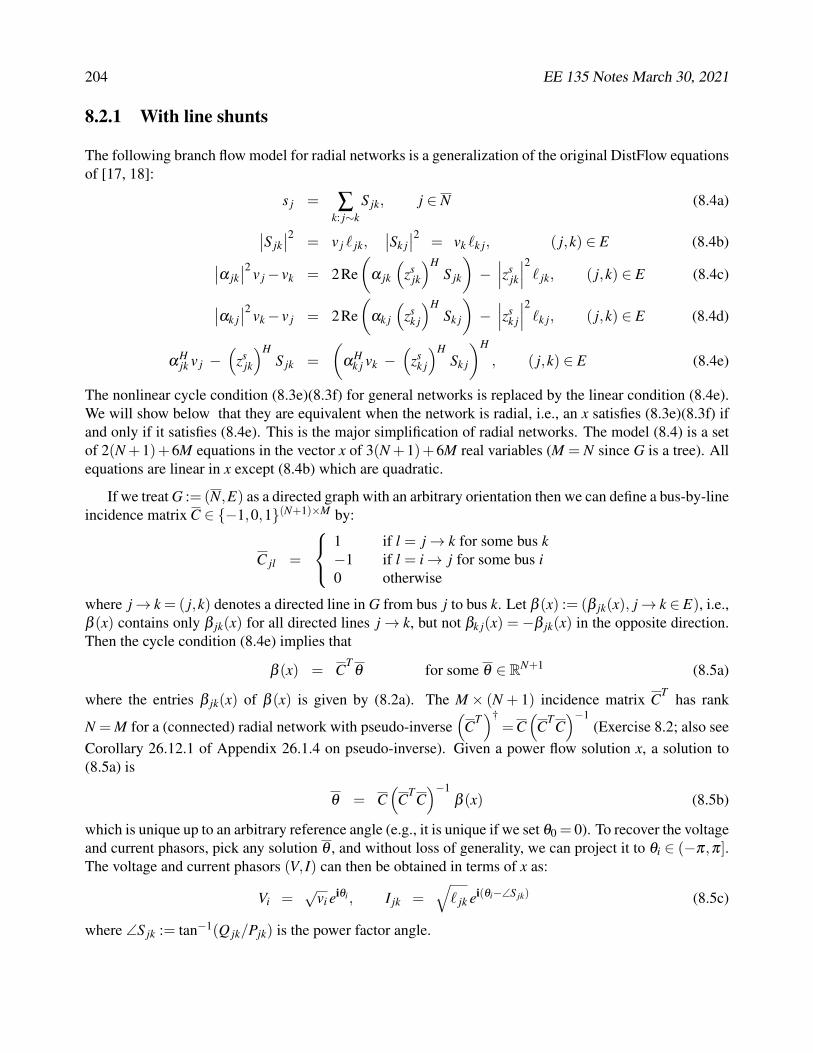
204 EE 135 Notes March 30, 2021

8.2.1 With line shunts

The following branch flow model for radial networks is a generalization of the original DistFlow equationsof [17, 18]:

s j = Âk: j⇠k

S jk, j 2 N (8.4a)

��S jk��2

= v j ` jk,��Sk j

��2= vk `k j, ( j,k) 2 E (8.4b)

��a jk��2 v j � vk = 2Re

✓a jk

⇣zs

jk

⌘HS jk

◆�

��zsjk

��2` jk, ( j,k) 2 E (8.4c)

��ak j��2 vk � v j = 2Re

✓ak j

⇣zs

k j

⌘HSk j

◆�

��zsk j

��2`k j, ( j,k) 2 E (8.4d)

aHjk v j �

⇣zs

jk

⌘HS jk =

✓aH

k j vk �⇣

zsk j

⌘HSk j

◆H, ( j,k) 2 E (8.4e)

The nonlinear cycle condition (8.3e)(8.3f) for general networks is replaced by the linear condition (8.4e).We will show below that they are equivalent when the network is radial, i.e., an x satisfies (8.3e)(8.3f) ifand only if it satisfies (8.4e). This is the major simplification of radial networks. The model (8.4) is a setof 2(N +1)+6M equations in the vector x of 3(N +1)+6M real variables (M = N since G is a tree). Allequations are linear in x except (8.4b) which are quadratic.

If we treat G := (N,E) as a directed graph with an arbitrary orientation then we can define a bus-by-lineincidence matrix C 2 {�1,0,1}(N+1)⇥M by:

C jl =

8<

:


where j ! k = ( j,k) denotes a directed line in G from bus j to bus k. Let b (x) := (b jk(x), j ! k 2 E), i.e.,b (x) contains only b jk(x) for all directed lines j ! k, but not bk j(x) = �b jk(x) in the opposite direction.Then the cycle condition (8.4e) implies that

b (x) = CT q for some q 2 RN+1 (8.5a)

where the entries b jk(x) of b (x) is given by (8.2a). The M ⇥ (N + 1) incidence matrix CT has rank

N = M for a (connected) radial network with pseudo-inverse⇣

CT⌘†

= C⇣

CTC⌘�1

(Exercise 8.2; also seeCorollary 26.12.1 of Appendix 26.1.4 on pseudo-inverse). Given a power flow solution x, a solution to(8.5a) is

q = C⇣

CTC⌘�1

b (x) (8.5b)

which is unique up to an arbitrary reference angle (e.g., it is unique if we set q0 = 0). To recover the voltageand current phasors, pick any solution q , and without loss of generality, we can project it to qi 2 (�p,p].The voltage and current phasors (V, I) can then be obtained in terms of x as:

Vi =p

vi eiqi , I jk =q

` jk ei(qi�\S jk) (8.5c)

where \S jk := tan�1(Q jk/Pjk) is the power factor angle.

EE 135 Notes March 30, 2021 205

8.2.2 Without line shunts

Consider a radial network with zero shunt admittances. A consequence of substituting ymjk = ym

k j = 0 into(8.4) for all lines ( j,k) 2 E is the relation between the sending-end power flows S jk and Sk j (see Exercise8.3):

S jk + Sk j = zsjk` jk = zs

jk`k j (8.6)

It says that the sum of sending-end power flows is equal to the complex line loss across the seriesimpedance zs

jk. We can use this relation to express `k j = ` jk and Sk j = zsjk` jk � S jk in terms of (` jk,S jk)

and eliminate branch variables (`k j,Sk j) in the opposite direction from (8.4). This leads to a simpler set ofequations based on a directed, rather than undirected, graph G, as we now explain.

In this subsection we assume G = (N,E) is directed. We denote a line in E from bus j to bus k either by( j,k) 2 E or j ! k 2 E. Associated with each line j ! k 2 E are branch variables (` jk,S jk) (and there arenot variables (`k j,Sk j) in the oposite direction). Let (s,v) := (si,vi, i 2 N) and (`,S) := (` jk,S jk, j ! k 2 E).Let x := (s,v,`,S) in R

3(N+1+M) with M = N since G is a tree. Without loss of generality we take bus 0as the root of the tree. Even though the graph orientation can be arbitrary we discuss two particularlyconvenient graph orientations: one where every line points away from bus 0 and the other where everyline points towards bus 0; see Figure 8.1. For every bus j there is a unique node i that is adjacent to j on

0

i

j

k

0

i

j

k

(a) All lines point away from bus 0 (b) All lines point towards bus 0

Figure 8.1: Notation for BFM for radial networks.

the path from bus 0 to bus j. We present two sets of power flow equations, one for each graph orientation.These two models are equivalent in the sense that there is a bijection F that maps x to x = F(x) such thatx is a solution to the first set of equations if and only if x is a solution to the second set of equations.Given a power flow solution x in either model, the voltage and current phasors can be obtained using(8.5) with a jk = 1 in the definition of b jk(x). To simplify notation we omit the superscript and write

z jk = (r jk,x jk) =⇣

ysjk

⌘�1as the series impedance of line ( j,k).

206 EE 135 Notes March 30, 2021

Down orientation: lines point away from bus 0. We now substitute `k j = ` jk and Sk j = zsjk` jk � S jk

into (8.4) to eliminate branch variables (`k j,Sk j) and obtain a simpler set of equations for BFM for a radialnetwork without line shunts:

Âk: j!k

S jk = Si j � zi jì j + s j, j 2 N (8.7a)

v j � vk = 2Re⇣

zHjkS jk

⌘� |z jk|2` jk, j ! k 2 E (8.7b)

v j` jk = |S jk|2, j ! k 2 E (8.7c)

where bus i denotes the unique adjacent node of j on the path from node 0 to node j, with the understandingthat when j = 0 then Si0 = 0 and ì0 = 0 in (8.7a). When j is a leaf node2, all S jk = 0 in (8.7a). Again thismodel adopts a directed graph where branch variables (` jk,S jk) are defined only for the direction of thelines j ! k 2 E, not for the opposite directions. The vector v includes v0 and s includes s0. This model isfirst proposed in [17, 18] for radial networks and is called the DistFlow equations.

Despite the complex notation, (8.7) is a set of 2(N + 1 + M) real equations in 3(N + 1 + M) realvariables x = (pi,qi,vi,` jk,Pjk,Q jk). They are a shorthand for:

Âk: j!k

Pjk =�Pi j � ri jì j

�+ p j, j 2 N

Âk: j!k

Q jk =�Qi j � xi jì j

�+q j, j 2 N

v j � vk = 2�r jkPjk + x jkQ jk

�� (r2

jk + x2jk)` jk, j ! k 2 E

v j` jk = P2jk +Q2

jk, j ! k 2 E

Since M = N, there are (4N + 2) equations in (6N + 3) real variables. Given (2N + 1) of these variables(e.g., given v0 = 1 and non-slack bus injections (p j,q j), j 2 N), the power flow problem is to determinethe remaining 4N +2 variables from these equations.

Up orientation: lines point towards bus 0. When the graph orientation is opposite to that in Case 1,BFM is specified by the following equations in x := (s, v, ˆ, S):

S ji = Âk:k! j

�Sk j � zk j ˆk j

�+ s j, j 2 N (8.8a)

vk � v j = 2Re⇣

zHk jSk j

⌘� |zk j|2 ˆk j, k ! j 2 E (8.8b)

vk ˆk j = |Sk j|2, k ! j 2 E (8.8c)

where i in (8.8a) denotes the node adjacent to j on the unique path between node 0 and node j. Theboundary condition is defined by S ji = 0 in (8.8a) when j = 0 and Sk j = 0,`k j = 0 in (8.8a) when j is aleaf node. For an advantage of this orientation see Remark 8.1.

2A node j is a leaf node if there exists no k such that j ! k 2 E.

EE 135 Notes March 30, 2021 207

General orientation. For general graph orientation, the power flow equations in x are:

Âk: j!k

S jk = Âi:i! j

�Si j � zi j`i j

�+ s j, j 2 N (8.9a)

v j � vk = 2Re⇣

zHjkS jk

⌘� |z jk|2` jk, j ! k 2 E (8.9b)

v j` jk = |S jk|2, j ! k 2 E (8.9c)

The power flow equations (8.9) for different graph orientations are the same, but their boundary conditionsmay be different.

Intuitively nodal injections and voltages (s,v) should not depend on the orientation of the graph whilebranch currents and power (`,S) do, since branch variables are defined only in the direction of the lines,not in the opposite direction. We can formally relate the power flow solutions defined for opposite graphorientations. Specifically, consider the opposite orientation where the direction of every line is reversedfrom that in (8.9). The resulting power flow equations are:

Âk: j!k

S jk = Âi:i! j

�Si j � zi j ˆi j

�+ s j, j 2 N (8.10a)

vk � v j = 2Re⇣

zHjkSk j

⌘� |z jk|2 ˆk j, k ! j 2 E (8.10b)

vk ˆk j = |Sk j|2, k ! j 2 E (8.10c)

An example is the down and up orientations above. Then it can be shown that there is a bijection g suchthat x is a power flow solution of (8.9) if and only if x := g(x) is a power flow solution of (8.10) (Exercise8.4). Indeed x = g(x) is given by:

s j := s j, v j := v j, ˆk j := ` jk, Sk j := ��S jk � z jk` jk

�(8.11)

An advantage of the up orientation above is illustrated in Chapter 8.4 in proving a simple bound on v j.Since v j = v j, this immediately implies a bound on v j as well, which would have been hard to provedirectly.

8.3 Equivalence

Equivalence. As presented in Chapters 8.1 and 8.2 the branch flow models are defined by the power flowequations:

1. For general networks: (8.1) or (8.3);

2. For radial networks with line shunts: (8.4);

3. For radial networks without line shunts (DistFlow equations): (8.7), (8.8).

Chapter 9

Linear models

9.1 DC power flow model

A popular linearized model, called the DC power flow model, makes the following assumptions:

• Lines are lossless, i.e., g jk = 0, so ysjk = ib jk for all lines ( j,k) 2 E, and there are no shunt elements

ymjk = 0 for all ( j,k) 2 E.

• Voltage angle differences are small across each line, i.e., sin(q j �qk) ' q j �qk for all lines ( j,k) 2 E.

• Voltage magnitudes |Vj| are given constants for all buses j 2 N.

• Ignore reactive power, so the variables in the DC power flow model are (p j,q j, j 2 N).

Under these assumptions, the DC power flow model is defined by (substituting g jk = 0 and replace sinq jkwith q j �qk in (7.18a)):

p j =N

Âk=0

b jk|Vj||Vk|(q j �qk) (9.1)

where b jk = 0 if j = k or if j 6= k and ( j,k) 62 E. Clearly Â j p j = Â j Âk b jk|Vj||Vk|(q j � qk) = 0. Thisis a consequence of the lossless assumption g jk = 0.

For many applications, such as economic dispatch (Chapter 18) and distribution factors and cascadingfailure analysis (Chapter 23), we use a vector form of the model (9.1), as follows. Let N := {0}[ N :={0,1, . . . ,N} be the set of |N| = N + 1 buses where we designate without loss of generality bus 0 as theslack bus. Let E ✓ N ⇥N be the set of |E| =: M lines connecting these buses. Let G := (N,E) be a directedgraph with an arbitrary orientation that represents the network topology.1 Let C 2 {�1,0,1}(N+1)⇥M be

1If G models an area of a multi-area interconnected power system then some of the buses in N represent the terminals oftie lines with other areas.

219

220 EE 135 Notes March 30, 2021

the bus-by-line incidence matrix defined by:

C jl =

8<

:


Unless otherwise specified we usually assume G is connected. Let B = diag(bl, l 2 E) be the (weighted)susceptance matrix with bl := |Vj||Vk|/b jk > 0 for link l = ( j,k), where |Vj|, |Vk| are (given) voltage mag-nitudes and b jk is the line susceptance.

Let p := (p j, j 2 N) be the net power injections at buses in N. Let q := (q j, j 2 N) be the voltagephase angles at these buses. Let P := (Pl, l 2 E) be the real power flows on line l. The DC power flowmodel is specified by the following equations in (p,Pq) to get

p = CP, P = BCT q (9.2a)

In many applications we are given the injections p and solve (9.2a) for a power flow solution (P,q).Eliminate P to relate voltage angles q directly to injections p:

p = CBCT q =: Lq

where the (N + 1)⇥ (N + 1) matrix L := CBCT is called the Laplacian matrix of the graph G. We willdiscuss many of its properties in Chapter 23.3. For now we note that, when G is connected, L has rank Nand the null space is span(1) where the (N +1)⇥(N +1) vector 1 whose entries are all 1’s is an eigenvectorof L corresponding to its eigenvalue l0 = 0. Let L† denote its Moore-Penrose pseudo-inverse (see Chapter26.1.4 for properties of pseudo-inverse). Given an injection vector p that is orthogonal to span(1), i.e.,power is balanced over the network 1T p = Â j2N p j = 0, the DC power flow equation (9.2a) has a solution(P,q) given by (see Exercise 9.4):

P = BCT L† p, q = L† p (9.2b)

This solution is unique up to an arbitrary reference angle q0. Therefore a more explicit description of DCpower flow solutions (P,q) is:

P = BCT L† p, q = L† p + a1, a 2 R (9.2c)

since 1 is in the null space of L. For example we can choose a so that q0 = 0 at the slack bus 0. It isimportant that the line flows P are unique regardless of the choice of q because CT 1 = 0.

Let C 2 {�1,0,1}N⇥M be the reduced incidence matrix obtained from C by removing the row corre-sponding to the slack bus 0. Let L := CBCT be the reduced Laplacian matrix. Hence L can be obtainedfrom L by removing row and column 0 corresponding to the slack bus. Then L is of rank N and invertible(see Theorem 9.3.4). Let A := L�1 denote its inverse. Let p := (p j, j 2 N) and q := (q j, j 2 N) be thepower injections and voltage angels at non-slack buses. Then the solution (P,q) can also be expressed interms of the (inverse A of the) reduced Laplacian matrix L.

Lemma 9.1. For any injections p with Â j2N p j = 0 we have

P = BCT L† p = BCT Ap, q = Ap (9.3)

This implies CT L† p = CT Ap.

EE 135 Notes March 30, 2021 221

Proof. Write

C =

cT

0C

�, p =

p0p

�, q =

q0q

�

where cT0 is the row of C corresponding to the slack bus 0. Then

L =

cT

0 Bc0 cT0 BCT

CBc0 L

�

with L = CBCT and the power flow equations (9.2a) become:

p0 = cT0 Bc0 q0 + cT

0 BCT q , p = CBc0 q0 + Lq

P = B⇥c0 CT ⇤

q0q

�= Bc0q0 + BCT q

The power flow solution (9.3) corresponds to choosing a in (9.2c) so that q0 = 0. Equating P in (9.2b) and(9.3) gives B�1P = CT L† p = CT Ap. This completes the proof.

The quantities in the lemma are illustrated in Exercise 9.5.

The DC power flow model is widely used in the industry, e.g., in economic dispatch of generators. Theassumptions are reasonable for many problems in transmission networks where the voltage magnitudesare high and real power losses are small. The last two assumption in the model are justified becauseon transmission networks where loss is low, there is decoupling between voltage angle q j and reactivepower qk and between voltage magnitude |Vj| and real power pk; see Chapter 3.2.5. Hence it is implicitlyassumed that reactive power injections qk can be chosen to stabilize the voltage magnitudes |Vj| separatelyfrom the determination of (p j,q j, j 2 N).

These assumptions are not suitable for distribution systems where voltages are much lower, the ratio ofline resistance to reactance is high, and reactive power is often used to stabilize voltages. We will describea different linearized model in Chapter ?? that is more suitable for distribution systems.

9.2 Laplacian matrix L

In this section we collect some basic properties of the Laplacian matrix that are useful in the analysis ofthe DC power flow model (9.2)(9.3). These properties are extensively used in the analysis of economicdispatch in Chapter 18 and distribution factors and cascading failure analysis in Chapter 23.

The entries of the Laplacian matrix L := CBCT are given by (Exercise 9.1):

Li j :=

8<

:

�bi j i ⇠ j (i 6= j)Âk⇠i bik i = j0 otherwise

The defining property of the Laplacian matrix L is that it is symmetric (because bi j = b ji), bl > 0 for alll 2 E, and all row sums are zero. This leads to the following important property from which many otherproperties of L follow.

Chapter 13

OPF and semidefinite relaxations: BIM

For our purposes an optimal power flow (OPF) problem is a mathematical program that seeks to minimizea certain function, such as total power loss, generation cost or user disutility, subject to the Kirchhoff’slaws as well as capacity, stability and security constraints. OPF is fundamental in power system operationsas it underlies many applications such as economic dispatch, unit commitment, state estimation, stabilityand reliability assessment, volt/var control, demand response, etc. There has been a great deal of researchon OPF since Carpentier’s first formulation in 1962 [54]. An early solution appears in [55] and extensivesurveys can be found in e.g. [56, 57, 58, 59, 60, 61, 62, 63, 64, 65, 66, 67, 68, 69, 70].

Power flow equations are quadratic and hence OPF can be formulated as a quadratically constrainedquadratic program (QCQP). It is nonconvex and has been shown to be NP-hard in general [71, 72, 73]. Alarge number of optimization algorithms and relaxations have been proposed. A popular approximationis a linear program, called DC OPF, obtained through the linearization of the power flow equations e.g.[74, 75, 76, 77, 78]. See also [20] for a more accurate linear approximation. To the best of our knowledgesolving OPF through semidefinite relaxation is first proposed in [79] as a second-order cone program(SOCP) for radial (tree) networks and in [80] as a semidefinite program (SDP) for general networks ina bus injection model. It is first proposed in [81, 26] as an SOCP for radial networks in the branch flowmodel of [17, 18]. See Remark 13.2 below for more details. While these semidefinite relaxations havebeen illustrated numerically in [79] and [80], whether or when they will turn out to be exact is first studiedin [72]. Exploiting graph sparsity to simplify the SDP relaxation of OPF is first proposed in [35, 36, 82]and analyzed in [83, 28].

Semidefinite relaxation of quadratic programs has been applied to many engineering problems; seee.g. [84]. There is a rich theory and extensive empirical experiences. Compared with other approaches,solving OPF through semidefinite relaxation offers several advantages. First, while DC OPF is useful in awide variety of applications, it is not applicable in other applications; see Remark 8.3. Second a solutionof DC OPF may not be feasible (may not satisfy the nonlinear power flow equations). In this case anoperator may tighten some constraints in DC OPF and solve again. This may not only reduce efficiencybut also relies on heuristics that are hard to scale to larger systems or faster control in the future. Third,when they converge, most nonlinear algorithms compute a local optimal usually without assurance on thequality of the solution. In contrast a semidefinite relaxation provides for the first time the ability to checkif a solution is globally optimal. If it is not, the solution provides a lower bound on the minimum cost and

281

282 EE 135 Notes March 30, 2021

hence a bound on how far any feasible solution is from optimality. Unlike approximations, if a relaxedproblem is infeasible, it is a certificate that the original OPF is infeasible.

13.1 OPF as QCQP

13.1.1 Preliminaries: QCQP and semidefinite relaxation

Quadratic constrained quadratic program (QCQP) is the following problem:

minx2Cn

xHC0x (13.1a)

subject to xHClx bl, l = 1, . . . ,L (13.1b)

where x 2 Cn, for l = 0, . . . ,L, Cl 2 S

n are Hermitian matrices so that xHClx are real values, and bl 2 R

are given. If Cl , l = 0, . . . ,L, are positive semidefinite (psd) then (26.27) is a convex QCQP. Otherwise itis generally nonconvex.

Any psd rank-1 matrix X 2 Cn⇥n has a spectral decomposition X = xxH for some x 2 C

n; see Chapter26.1.3. The factor x is unique up to a rotation, i.e., x satisfies X = xxH if and only if xe jq for any q 2 R.Using xHClx = tr ClxxH =: tr ClX we can rewrite a QCQP as the following equivalent problem where theoptimization is over Hermitian matrices:

minX2Sn

tr C0X (13.2a)

subject to tr ClX bl, l = 1, . . . ,L (13.2b)X ⌫ 0, rank X = 1 (13.2c)

While the objective function and the constraints in (26.27) are quadratic in x they are linear in X in(26.28a)–(26.28b). The constraint X ⌫ 0 in (26.28c) is convex (Sn

+ is a convex cone). The rank con-straint in (26.28c) is the only nonconvex constraint. Removing the rank constraint results in a semidefiniteprogram (SDP):

minX2Sn

tr C0X (13.3a)

subject to tr ClX bl, l = 1, . . . ,L (13.3b)X ⌫ 0 (13.3c)

SDP is a convex program and can be efficiently computed. We call (26.29) an SDP relaxation of QCQP(26.27) because the feasible set of the equivalent problem (26.28) is a subset of the feasible set of SDP(26.29). A strategy for solving QCQP (26.27) is to solve SDP (26.29) for an optimal Xopt and check itsrank. If rank Xopt = 1 then Xopt is optimal for (26.28) as well and an optimal solution xopt of QCQP (26.27)can be recovered from Xopt through spectral decomposition Xopt = xopt(xopt)H . If rank Xopt > 1 then, ingeneral, no feasible solution of QCQP can be directly obtained from Xopt but the optimal objective valueof SDP provides a lower bound on that of QCQP.

EE 135 Notes March 30, 2021 283

13.1.2 OPF formulation

For our purposes an optimal power flow (OPF) problem is a constrained optimization that minimizes acertain cost function subject to two sets of constraints. It is fundamental because it underlies numerouspower system operation and planning applications. The first set of constraints are the power flow equa-tions discussed in Chapter 7.2. The second set of constraints are operational constraints. The cost functionand the operational constraints depend on the application for which the OPF problem is studied. In thisbook we will only consider the simplest OPF with a small number of operational constraints. We also re-strict ourselves to applications that involve only continuous variables or where any discrete variables havebeen relaxed to continuous variables. Many applications, e.g., unit commitment, transmission switching,involve discrete variables and solving mixed integer programs is an important and difficult topic in itself.

For power flows as equality constraints in OPF we will use for notational simplicity the complex form(7.17) reproduced here: 1

s j = Âk: j⇠k

yHjk�|Vj|2 �VjV H

k�

+ yHj j |Vj|2, j 2 N (13.4)

where y jk are the series admittances of lines ( j,k) and y j j are the total line shunt admittances incident onbuses j. The most common operational constraints are:

• Constraints on power injections (e.g., generation or load capacity limits):

s j s j s j, j 2 N (13.5)

where s j and s j are given bounds on the injections at buses j.2

• Constraints on voltage magnitudes:

v j |Vj|2 v j, j 2 N (13.6)

where v j and v j are given lower and upper bounds on the squared voltage magnitudes. We assumev j > 0 to avoid triviality.

• Constraints on branch power flows

S jk S jk(V ) S jk, ( j,k) 2 E (13.7)

Here the branch power flows S jk(V ) are functions of V (from (7.15)):

S jk := VjIHjk =

⇣ys

jk


k�

+⇣

ymjk

⌘H|Vj|2

and hence (13.7) are quadratic constraints on the voltage phasors V . Instead of (13.7) an alternativeis to impose constraints on the apparent power:

|S jk(V )| S jk, ( j,k) 2 E

1We sometimes omit the superscript in ysjk or ym

j j when there is no danger of confusion. We will always retain the superscriptwhen referring to ys

jk and ymjk in the same discussion to avoid confusion.

2All variables are complex and, by a a where a,a 2 C, we mean separate bounds on the real and imaginary parts,Re a Re a and Im a Im a.

284 EE 135 Notes March 30, 2021

These constraints are polynomial in Vj and can be converted into quadratic constraints possibly in alifted space.

• Constraints on squared branch current magnitudes (from (7.3)):��ys

jk(Vj �Vk) + ymjk Vj

��2

I2jk, ( j,k) 2 E (13.8)

Usually either constraints (13.7) or (13.8) are included.

This is a general formulation that includes power injections s j and voltages Vj at every bus j. If there isno bound on the injection at bus j then s j := �• � i• or s j := • + i•. On the other hand the inequalityconstraints also allow the case where a quantity is not an optimization variable but a parameter by settings j = s j to the specified value. For instance s j = s j = s j may represent a given constant-power load. Forthe slack bus 0, unless otherwise specified, we always assume v0 = v0 = 1 and s0 = �•� i•, s0 = •+ i•.Therefore we sometimes replace j 2 N in (13.5) and (13.6) by j 2 N.

We can eliminate the injection variables s j by substituting (13.4) into (13.5) and replace it by:

s j Âk: j⇠k


k�

+ yHj j |Vj|2 s j, j 2 N (13.9)

Define the feasible set of OPF to be:

V := {V 2 Cn+1 | V satisfies (13.9)(13.6)(13.7) and/or (13.8)} (13.10)

Denote the cost function by C0(V ). Typical costs include the cost of generation (e.g. in economicdispatch), estimation error (e.g. in state estimation), line loss (e.g. in volt/var control in distributionsystems), and user disutility (e.g., in demand response). All these costs can be expressed as functions ofV . For instance to minimize weighted sum of real power generations we can use (from (13.4))

C0(V ) := Âgenerators j

Re s j = Re

Âk: j⇠k


k�

+ yHj j |Vj|2

!

To reduce the total thermal loss we can use (from (7.3))

C0(V ) := Â( j,k)2E

r jk |I jk|2 = Â( j,k)2E

r jk

��ysjk(Vj �Vk) + ym

jkVj

��2

Then OPF in the bus injection model can then be defined as:OPF:

minV

C0(V ) subject to V 2 V (13.11)

We now assume the cost function C0(V ) := V HC0V is quadratic in V for some Hermitian matrix C0.Similarly we can express OPF constraints as quadratic forms in V . To express the injection s j as a quadraticform note that

s j = VjIHj = (eH

j V )(IHe j) = tr�eH

j V IHe j�

EE 135 Notes March 30, 2021 285

where e j is the (n + 1)-dimensional vector with 1 in the jth entry and 0 elsewhere. Substitute I = YV towrite (using tr(AB) = tr(BA))

s j = tr�eH

j VV HY He j�

= tr��

Y He jeHj�

VV H� = V HY Hj V

where Yj := e jeHj Y is an (n + 1)⇥ (n + 1) matrix with its jth row equal to the jth row of the admittance

matrix Y and all other rows equal to the zero vector. Yj is not Hermitian so that V HY Hj V is in general

a complex number. Its real and imaginary parts can be expressed in terms of the Hermitian and skewHermitian components of Y H

j defined as:

F j :=12�Y H

j +Yj�

and Y j :=12i�Y H

j �Yj�

Then F j and Y j are Hermitian matrices and

Re s j = V HF jV and Im s j = V HY jV

They will be upper and lower bounded by

p j := Re s j and p j := Re s j

q j := Im s j and q j := Im s j

We will write (13.9) in terms of these quantities in the OPF formulation below.

Let Jj := e jeHj denote the Hermitian matrix with a single 1 in the ( j, j)th entry and 0 everywhere else.

Then squared voltage magnitude |Vj|2 = V HJjV is a quadratic form. It will be lower and upper boundedby v j and v j respectively. We can also express the squared branch current |I jk|2 and power flow S jk(V ) asquadratic forms in V . Recall from (7.3)

I jk = ysjk(Vj �Vk) + ym

jkVj =⇣

ysjk(e j � ek)

T + ymjk eT

j

⌘V

Hence |I jk|2 = Y HYjkY , which will be upper bounded by I2jk, where

Yjk :=⇣

ysjk(e j � ek)

T + ymjk eT

j

⌘H ⇣ys

jk(e j � ek)T + ym

jk eTj

⌘

The matrix Yjk is Hermitian. Using the expression of I jk, S jk(V ) in quadratic form is:

S jk(V ) = VjIHjk =

�eH

j V�⇣

ysjk(e j � ek)

TV + ymjk eT

j V⌘H

= eHj�VV H�

✓⇣ys

jk + ymjk

⌘He j �

⇣ys

jk

⌘Hek

◆

= tr�Yjk

�VV H�� = V HYjkV

where

Yjk :=✓⇣

ysjk + ym

jk

⌘He j �

⇣ys

jk

⌘Hek

◆eH

j

286 EE 135 Notes March 30, 2021

Yjk is not Hermitian. Define

F jk :=12

⇣Y H

jk + Yjk

⌘and Y jk :=

12i

⇣Y H

jk � Yjk

⌘

so that

Re S jk = V HF jkV and Im S jk = V HY jkV

They will be upper and lower bounded by

P jk := Re S jk and P jk := Re S jk

Q jk := Im S jk and Q jk := Im S jk

Then OPF (13.11) can be written as a standard form quadratic constrained quadratic program (QCQP):

minV2Cn+1

V HC0V (13.12a)

subject to p j V HF jV p j, j 2 N (13.12b)

q j V HY jV q j, j 2 N (13.12c)

v j V HJjV v j, j 2 N (13.12d)

P jk V HF jkV P jk, ( j,k) 2 E (13.12e)

Q jk V HY jkV Q jk, ( j,k) 2 E (13.12f)

V HYjkV I2jk, ( j,k) 2 E (13.12g)

13.2 NP hardness

Since the feasible set V of OPF is generally a nonconvex set, OPF formulated in (13.11) or (13.12) is anonconvex problem and has been shown to be NP-hard.

13.3 Relaxations of QCQP

In this section we derive semidefinite relaxations of OPF and clarify their relations. The cost functionC(V ) of OPF is usually assumed to be convex in its variables. The difficulty of OPF formulated herethus arises from the nonconvex feasible set V of OPF. Informally one can regard a relaxation of OPF asminimizing the same cost function over a convex superset (though in a lifted space). Different choicesof convex supersets lead to different relaxations, but they all provide lower bounds to OPF. If an optimal

EE 135 Notes March 30, 2021 287

solution of a relaxation happens to lie in V then it is also feasible and hence optimal for the original OPF.In this case we say the relaxation is exact.

In this section we present three characterizations of the feasible set V in BIM. These characterizationsnaturally suggest convex supersets and semidefinite relaxations of OPF, and we prove equivalence relationsamong them. In the next section we present sufficient conditions that guaranteed exact relaxations.

13.3.1 SDP elaxations

The OPF (13.12) takes the form of a standard QCQP:

minV2Cn

V HC0V subject to V 2 V (13.13a)

where the feasible set

V := {V 2 Cn |V HClV bl, l = 1, . . . ,L} (13.13b)

and C0 is a positive semidefinite (psd) matrix and Cl , l � 1, are Hermitian matrices.3 In this subsectionwe develop semidefinite relaxations of general QCQP (13.13). In the next subsection we apply it to ourOPF problem (13.12).

We now apply the SDP relaxation explained in Chapter 13.1.1 to OPF. Recall that V HMV = tr MVV H =tr MW for the psd rank-1 matrix W = VV H . This suggests the following equivalent problem:

minW2Sn

tr CW subject to W 2 W (13.14a)

where Sn is the set of Hermitian matrices and the feasible set

W := {W 2 Sn | tr ClW bl, l = 1, . . . ,L, W ⌫ 0, rank W = 1} (13.14b)

These two problems are equivalent in the sense that, given a feasible (or optimal) solution V to QCQP(13.13), there is a unique W := VV H that is feasible (or optimal) to the semidefinite program (13.14).Conversely, given an W that is feasible (or optimal) to (13.14), a unique solution V to (13.13) can berecovered through rank-1 factorization W = VV H (V is unique up to a rotation eiq ). It is in this sense thatwe say the sets V and W are equivalent, written as V ⌘ W.

Whereas (13.13) is quadratic in V the equivalent problem (13.14) is convex in W except the nonconvexrank-1 constraint. Removing the rank-1 constraint from (13.14) yields the following convex relaxation:

minW2Sn

tr CW subject to W 2 W+ (13.15a)

where the feasible set

W+ := {W 2 S

n | tr ClW bl, l = 1, . . . ,L, W ⌫ 0} (13.15b)

3In this subsection we abuse notation and use n,m to denote general integers unrelated to the number of buses or lines in apower network.

288 EE 135 Notes March 30, 2021

We will refer to (13.15) as the SDP relaxation of QCQP (13.13). Its feasible set W+ of the semidefinite

relaxation is a superset of W which is equivalent to the feasible set V of the original QCQP. This is referredto as lifting the original QCQP problem from n dimensional space C

n to the higher-dimensional space ofn⇥n psd matrices where the problem is simpler.

Even though the relaxation (13.15) is a convex problem computing its solution can still be challengingif the problem size n is large. Computation can be greatly simplified by exploiting the sparsity of theunderlying network. To derive the simpler chordal and second-order cone program (SOCP) relaxations ofQCQP we need to characterize the feasible set V in terms of partial matrices.

13.3.2 Exploiting graph sparsity

13.3.2.1 Partial matrices and completions

The matrices Cl , l = 0,1, . . . ,L, define an underlying undirected graph F := (N,E) with n nodes andm edges where distinct nodes j and k are adjacent (i.e., ( j,k) 2 E) if and only if there exists an l 2{0,1, . . . ,L} such that [Cl] jk 6= 0. Assume without loss of generality that the graph F is connected. Forany V 2 C

n note that the quadratic forms V HClV depends on |Vj|2 and on V Hj Vk if and only if ( j,k) 2 E is

a link in F , i.e., if and only if there exists an l such that the coefficient of V Hj Vk is nonzero:

V HClV = Âj,k

[Cl] jk V Hj Vk = Â

j[Cl] j j|Vj|2 + Â

( j,k)2E[Cl] jkVjV H

k

Hence the constraints V HClV bl do not depend on V Hj Vk if ( j,k) 62 E for any l. Correspondingly, Wjk of

the lifted variable W are not directly constrained by tr ClW bl if ( j,k) 62 E. This can be used to relax thepsd and rank-1 constraints on the entire matrix W , greatly the simplifying computation if the underlyinggraph F of the QCQP is sparse. To develop these ideas precisely we need definitions of partial matricesand their completions; see e.g. [88, 89, 90] for more details.

A partial matrix WF is a set of 2m+n complex numbers defined on F :

WF :=�

[WF ] j j, [WF ] jk, [WF ]k j | nodes j and edges ( j,k) of F

WF can be interpreted as a matrix with entries partially specified by these complex numbers. If F is acomplete graph (in which there is an edge between every pair of vertices) then WF is a fully specified n⇥nmatrix. A completion W of WF is any fully specified n⇥n matrix that agrees with WF on graph F , i.e.,

[W ] j j = [WF ] j j, [W ] jk = [WF ] jk for j,( j,k) 2 F

Given an n⇥n matrix W we use WF to denote the submatrix of W on F, i.e., the partial matrix consistingof the entries of W defined on graph F . If q is a clique (a fully connected subgraph) of F then let WF(q)denote the fully-specified principal submatrix of WF defined on q. We extend the trace operation to partialmatrices XF :

tr ClWF = Âj2N

[Cl] j j [WF ] j j + Â( j,k)2E

[Cl] jk [WF ] jk

Power Systems Analysis - Caltech Computer Science

Documents

Transcript of Power Systems Analysis - Caltech Computer Science