Texts in Computer Science

EditorsDavid GriesFred. B. Schneider

www.springer.com/series/3191For other titles published in this series, go to

David Salomon

The Computer GraphicsManual

Series EditorsDavid GriesDepartment of Computer ScienceUpson HallCornell UniversityIthaca, NY 14853-7501, USA

Fred. B. SchneiderDepartment of Computer ScienceUpson HallCornell UniversityIthaca, NY 14853-7501, USA

British Library Cataloguing in Publication DataA catalogue record for this book is available from the British Library

Apart from any fair dealing for the purposes of research or private study, or criticism or review, as

stored or transmitted, in any form or by any means, with the prior permission in writing of thepublishers, or in the case of reprographic reproduction in accordance with the terms of licenses issued bythe Copyright Licensing Agency. Enquiries concerning reproduction outside those terms should be sentto the publishers.

permitted under the Copyright, Designs and Patents Act 1988, this publication may only be reproduced,

The use of registered names, trademarks, etc., in this publication does not imply, even in the absence of aspecific statement, that such names are exempt from the relevant laws and regulations and therefore freefor general use.The publisher makes no representation, express or implied, with regard to the accuracy of the informationcontained in this book and cannot accept any legal responsibility or liability for any errors or omissionsthat may be made.

Printed on acid-free paper

DOI 10.1007/978- -8 - -7

ISSN 1868-0941 e-ISSN 1868-095XISBN 978-0-85729-885-0 e-ISBN 978-0-85729-886-7

Springer London Dordrecht Heidelberg New York

Library of Congress Control Number: 2011937970

Springer is part of Springer Science+Business Media (www.springer.com)

© Springer-Verlag London Limited 2011

Prof. David Salomon (emeritus)

California State UniversityNorthridge, CA 91330-8281, USAdsalomon@csun.edu

0 5729 886

Department of Computer Science

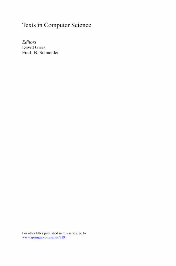
Plate A.2. A Cluttered Room, Day and Night (Live Interior).

To users of computer graphics everywhere

There’s no better sensation than image. It’s so in-your-face!

—Jimmy Lai

Preface

The field of quantum mechanics is the cornerstone of modern physics. This field wasrapidly developed in the 1920s and 1930s by a small group of (mostly young) researchers.They generally agreed that we cannot (and indeed, should not even try to) visualizeatoms, photons, and elementary particles. These objects, their attributes and theirbehavior are best described in terms of mathematical abstractions, not pictures. Indeed,one of the first textbooks in this area The Principles of Quantum Mechanics by P. A.M. Dirac, does not include a single diagram in its 314 pages.

This style of writing reflects one extreme approach to graphics, namely consideringit irrelevant or even detracting as a teaching tool and ignoring it. Today, of course,this approach is unthinkable. Graphics, especially computer graphics, is commonly usedin texts, advertisements, and videos to illustrate concepts, to emphasize points beingdiscussed, and to entertain.

Our approach to graphics has been completely reversed since the 1930s, and it seemsthat much of this change is due to the wide use of computers. Computer graphics todayis a mature, successful, and growing field. It is employed by many people for manypurposes and it is enjoyed by even more people. One criterion for the maturity of a fieldof study is its size. When a certain discipline becomes so big that no one person cankeep all of it in their head, we say that that discipline has matured (or has come of age).This is what happened to computer graphics in the last decade or so. It is now a largefield consisting of many subfields such as curve and surface design, rendering methods,and computer animation. Even a person who has written a book covering the entirefield cannot claim that they keep all that material in their head all the time, which isprecisely the reason why textbooks are being written.

In its 357 pages, The Principles of Quantum Mechanics featured neither a singlediagram, nor an index, nor a list of references, nor suggestions for further reading.

—Graham Farmelo, The Strangest Man, 2009.

vii

viii Preface

Overview and Goals

Today (in 2011), the power of computer-generated images is everywhere. Computergraphics has pervaded our lives to such an extent that sometimes we don’t even realizethat an image we are watching is artificial. The average person comes into contactwith computer graphics mostly in three areas, computers, television, and electronicdevices. Current computers and operating systems are based on GUI (graphical userinterface). Computer programs often display results graphically. Television programsand commercials employ sophisticated, computer-generated graphics that are often hardto distinguish from the real thing. Many television programs (mostly documentaries) andrecent movies mix real actors and artificial imagery to such an extent that the viewer mayfind it difficult to distinguish a real object or scene from a computer-generated image. (Areal actor trying to outrun a computer-generated dinosaur is a common example.) Moreand more digital cameras, electronic devices, and instruments have small screens thatdisplay messages, options, controls, and results in color and are often touch sensitive,enabling the user to enter commands by finger gesturing instead of from the traditionalkeyboard. Many cell telephones even have two screens, and some new digital camerasalso feature two LCD displays.

With this in mind, the goal of this manual is to present the reader with a widepicture of computer graphics, its history and its pioneers, the hardware tools it employs,and most important, the techniques, approaches, and algorithms that are at the coreof this field. Thus, this textbook/reference tries to describe as many concepts andalgorithms as possible, paying special attention to the important ones.

It would have been nice to include everything in this book and title it, like othertexts by the same author, Computer Graphics: The Complete Reference, but computergraphics has grown to a point where I cannot hope to be an authority on the entire field,which is why some readers may not find every topic, term, concept, and algorithm theymay be looking for.

New material for Volume 4 will first appear in beta-test form as fascicles of approx-imately 128 pages each, issued approximately twice per year. These fascicles willrepresent my best attempt to write a comprehensive account; but computer sciencehas grown to the point where I cannot hope to be an authority on all the materialcovered in these books. Therefore I’ll need feedback from readers in order to preparethe official volumes later.

—Donald E. Knuth.

On the other hand, those same readers may find in this manual/textbook topicsthey did not know existed, which might serve as compensation.

The many examples and exercises sprinkled throughout the book enhance its use-fulness. By paying attention to the examples and working out the exercises, readers willgain deeper understanding of the material.

Organization and Features

This manual is large and is organized in seven parts as follows:Part I covers the history, basic concepts, and techniques used in computer graphics.

The concepts of pixel, vector scan, and raster scan are discussed. It is shown how an

Preface ix

image given as a bitmap of pixels can be scaled (zoomed) and rotated. Many importantscan-conversion methods are explained and illustrated.

Part II is devoted to transformations and projections. It starts with the importanttwo- and three-dimensional transformations, including translation, rotation, reflection,and shearing. This is followed by the main types of projections, namely parallel, per-spective, and nonlinear.

Part III is by far the largest. It includes many methods, algorithms, and techniquesemployed to construct curves and surfaces, which are the building blocks of solid objects.Six important interpolation and approximation methods for curves and surfaces areincluded, as well as sweep surfaces and subdivision methods for surface design.

Part IV goes into advanced techniques such as rendering an object, eliminatingthose parts that are hidden from view, and bringing objects to life (animating them) byinterpolation. Several chapters included in this part discuss the nature and propertiesof light and color, graphics standards and graphics file formats, and fractals.

Part V describes the principles of image compression. It concentrates on two im-portant approaches to this topic, namely orthogonal and subband (wavelet) transforms.The important JPEG image compression standard is described in detail.

Part VI is devoted to many of the important input/output graphics devices. Chap-ter 26 describes them and explains their operations.

Part VII consists of appendixes, most of which discuss certain mathematical con-cepts.

The following features enhance the usefulness and appearance of this textbook:

The powerful MathematicaTM and Matlab software systems are used throughout thebook to implement the various concepts discussed. When a figure is computed in oneof these programs, the code is listed with the figure. These codes, which are availablein the book’s website, are meant to be readable rather than efficient and fast, and aretherefore easy to read and to modify even by inexperienced Mathematica and Matlabusers.

The book has many examples. Experience shows that examples are importantfor a thorough understanding of the kind of material discussed in this manual. Theconscientious reader should follow each example carefully and try to work out variationsof the examples. Many examples also include Mathematica code.

The many exercises sprinkled throughout the text are not a cosmetic feature. Theydeal with important topics, and should be worked out. Answers are provided but theyshould be consulted only as a last resort.

A quotation is a phrase that reflects its author’s profound thoughts. Quotationsand epigrams enliven a book, which is why they have been generously used throughoutthis manual. I hope that they add to the book and make it more interesting.

The ability to quote is a serviceable substitutefor wit.

—W. Somerset Maugham.

This manual/textbook aims to be practical, not theoretical. After reading andunderstanding a topic, the reader should be able to design and implement the concepts

x Preface

discussed there. The few mathematical arguments found in the book are simple, andthere is no attempt to present an overall theory encompassing the entire field of computergraphics.

An important feature of this text is the attention paid to orphans. Those aretopics that most texts on computer graphics either mention briefly or disregard com-pletely. Examples are perspective projections, nonlinear projections, nonlinear bitmaptransformations, curves, surfaces, I/O devices, and image compression. The reader willfind that this manual discusses orphans in great detail, including numerous examplesand exercises.

Most of the necessary mathematical background (such as vectors and matrices) iscovered in the Appendixes. However, some math concepts that are used only once (suchas the mediation operator and points vs. vectors) are discussed right where they areintroduced.

The Two Volumes

This textbook/reference is big because the discipline of computer graphics is big.There are simply many topics, techniques, and algorithms to discuss, explain, and illus-trate by examples. Because of the large number of pages, the book has been produced intwo volumes. However, this division of the book into volumes is only technical and thebook should be considered a single unit. It is wrong to consider volume I as introductoryand volume II as advanced, or to assume that volume I is important while volume II isnot. The volumes are simply two halves of a single, large entity.

The Color Plates

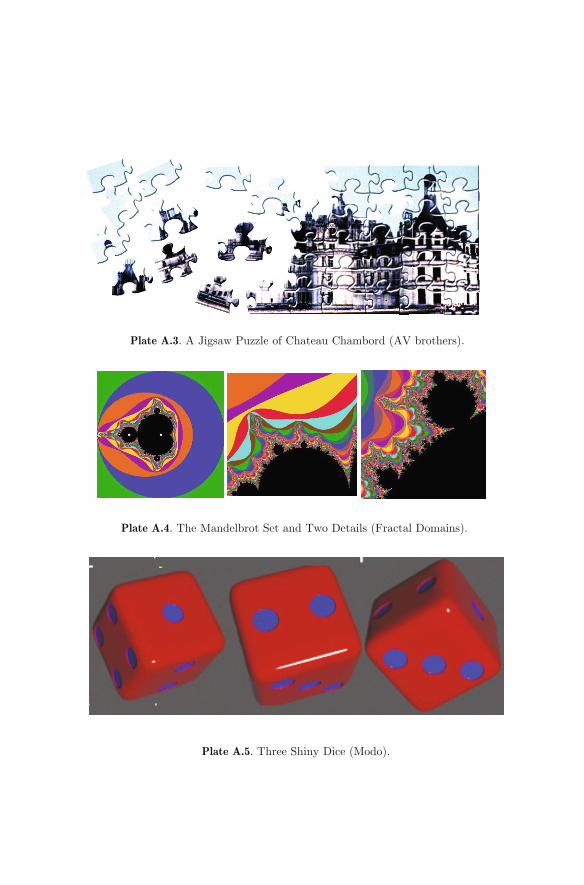
This extensive manual features more than 100 color plates, placed at the verybeginning, at the end, and between individual parts. They serve to liven up the bookand to illustrate many of the topics discussed. It is planned to place information aboutthese plates in the book’s website, for the benefit of readers who want to recreate orextend them. The plates were prepared over several months, using a variety of graphicssoftware. Appendix F has more information about the plates, their content, and thegraphics applications used to generate them.

A Word on Notation

It is common to represent nonscalar quantities such as points, vectors, and matrices withboldface. Here are examples of the notation used in this manual:

x, y, z, t, u, v Italics are used for scalar quantities such as coordinatesand parameters.

P, Qi, v, M Boldface is used for points, vectors, and matrices.

�CP An alternative notation for vectors, used when the twoendpoints of the vector are known.

Preface xi

P(t), P(u, v) Boldface with arguments is used for nonscalar functionssuch as curves and surfaces.

(a11 a12

a21 a22

)Parentheses (and sometimes square brackets) are used formatrices.

a11 a12

a21 a22Vertical bars are used for determinants.

|v| The absolute value (length) of vector v.

AT The transpose of matrix A.

x∗, P∗ The transformed values of scalars and points.

fu(u), Pt(t), Ptt(t) The derivatives (first, second,. . . ) of scalar and vector func-tions.

df(u)du

,dP(t)dt

Alternative notation for derivatives.

df2(u)du2

,dP2(t)dt2

Alternative notation for higher-order derivatives.

∂f(u, v)∂u

,∂P(u, v)

∂vPartial derivatives.

f(x)|x0 or f(x0) Value of function f(x) at point x0.

n∑i=1

xi The sum x1 + x2 + · · · + xn.

n∏i=1

xi The product x1x2 . . . xn.

� Exercise 1: What is the meaning of (P1,P2,P3,P4)?

Target Audiences

The material presented here has been developed over many years of teaching com-puter graphics. It has been revised, updated, and distilled many times, with manyfigures, examples, and exercises added. The text emphasizes the simplicity of the math-ematics behind computer graphics and tries to show how graphics software works andhow current computer graphics can generate and display realistic-looking curves, sur-faces, and solid objects. The key ideas are introduced slowly, are examined, whenpossible, from several points of view, and are illustrated and illuminated by figures,examples, and (solved) exercises. The discussion must employ mathematics, but it is

xii Preface

mostly non-rigorous (no theorems or proofs) and therefore easy to grasp. The math-ematical background required includes polynomials, matrices, vector operations, andelementary calculus. This manual/textbook was written with three groups of readers inmind.

Textbook/student. The book can serve as the primary text for a two-semesterclass on computer graphics for graduate and advanced undergraduate students. Themany fragments of Mathematica code found here may serve as a core around which stu-dents can build larger programs. The exercises are especially valuable for students, andthe lack of rigorous theorems and proofs should encourage those who consider computerscience distinct from mathematics.

Reference/professional use. Professionals in engineering, computers, and otherscientific disciplines generate, watch, and process digital images all the time. They oftenwould like to know more about how such images are generated. Artists, photographers,and publishing professionals use computer graphics routinely and may be interested in asolid background in this field. Those readers can benefit from two features of this book,namely the detailed index and the thorough and precise exposition of the principles,methods, and techniques used in computer graphics. This textbook/reference tries tocover all the important topics of the graphics field, some in more detail than others. Theindex is exceptionally detailed and constitutes 2.5% of the book.

Individuals/handy resource. All of us, not just certain professionals, are con-stantly exposed to digital images, digital effects, and computer animation. Intelligentpersons who try to widen their horizons may wonder how digital images are created,edited, and distributed. It is my belief that this manual can serve the needs of thisgroup of individuals as well. The book may prove useful to them because of the simple,straightforward descriptions of graphics devices and processes. The book may also be ahandy resource because of the detailed index, which makes it easy to locate any topic.

Supplementary Resources

Because of the importance of computer graphics, a vast number of supplementaryresources is available. Section 1.5 has a long list of seven classes of resources and this onlyscratches the surface of what is available. The Internet has many thousands of resourcesin the form of websites dedicated to graphics, class notes, scientific publications, andsoftware.

Please bear in mind that graphics, like any discipline associated with computersand computations, develops continually, so readers should search the Internet for new,useful, and exciting sources of information. Search items may be as general as “com-puter graphics,” “computer animation,” “image processing,” “computer vision,” and“computer-aided design (CAD),” or as specific as “how to twirl in Photoshop,” “whatis quaternion rotation,” and “Java code for dithering.”

Shaw’s plays are the price we pay for Shaw’s prefaces.

—James Agate.

Preface xiii

Acknowledgements

A book of this magnitude is generally written with the help, dedicated work, andencouragement of many people, and this large textbook/reference is no exception. Firstand foremost should be mentioned my editor, Wayne Wheeler and the copyeditor,Francesca White. They made many useful comments and suggestions, and pointedout many mistypes, errors, and stylistic blemishes. In addition, I would like to thankH. L. Scott for permission to use Figure 2.82, CH Products for permission to use Fig-ure 26.24b, Andreas Petersik for Figure 6.61, Shinji Araya for Figure 7.27, Dick Termesfor many figures and paintings, the authors of Hardy Calculus for the limerick at theend of Chapter 13, Bill Wilburn for many Mathematica notebooks, and Ari Salomon forphotos and panoramas in several plates.

I welcome any comments, suggestions and corrections. They should be emailed todsalomon@csun.edu. An errata list and other information will be maintained in thebook’s website http://www.davidsalomon.name/CGadvertis.

And now, to the matter at hand.

This preface made me so impatient, being conscious of my

own merits and innocence, that I was going to interrupt;

when he entreated me to be silent, and thus proceeded.

— Jonathan Swift, Gulliver’s Travels

Contents

Preface vii

Introduction 1

Part I Basic Techniques 7

1 Historical Notes 91.1 Historical Survey 91.2 History of Curves and Surfaces 131.3 History of Video Games 141.4 Pioneers of Computer Graphics 171.5 Resources For Computer Graphics 19

2 Raster Graphics 292.1 Pixels 302.2 Graphics Output 322.3 The Source-Target Paradigm 402.4 Interpolation 412.5 Bitmap Scaling 452.6 Bitmap Stretching 462.7 Replicating Pixels 462.8 Scaling Bitmaps with Bresenham 482.9 Pixel Art Scaling 542.10 Pixel Interpolation 562.11 Bilinear Interpolation 572.12 Interpolating Polynomials 582.13 Adaptive Scaling by 2 652.14 The Keystone Problem 732.15 Bitmap Rotation 762.16 Nonlinear Bitmap Transformations 792.17 Circle Inversion 852.18 Polygons (2D) 882.19 Clipping 91

xv

xvi Contents

2.20 Cohen–Sutherland Line Clipping 922.21 Nicholl–Lee–Nicholl Line Clipping 932.22 Cyrus–Beck Line Clipping 952.23 Sutherland–Hodgman Polygon Clipping 972.24 Weiler–Atherton Polygon Clipping 992.25 A Practical Drawing Program 1002.26 GUI by Inversion Points 1042.27 Halftoning 1072.28 Dithering 1092.29 Stippling 1182.30 Random Numbers 1222.31 Image Processing 1262.32 The Hough Transform 131

3 Scan Conversion 135

3.1 Scan-Converting Lines 1353.2 Midpoint Subdivision 1363.3 DDA Methods 1373.4 Bresenham’s Line Method 1423.5 Double-Step DDA 1473.6 Best-Fit DDA 1513.7 Scan-Converting in Parallel 1533.8 Scan-Converting Circles 1563.9 Filling Polygons 1673.10 Pattern Filling 1753.11 Thick Curves 1773.12 General Considerations 1793.13 Antialiasing 1803.14 Convolution 192

Part II Transformations and Projections 193

4 Transformations 199

4.1 Introduction 2014.2 Two-Dimensional Transformations 2044.3 Three-Dimensional Coordinate Systems 2324.4 Three-Dimensional Transformations 2334.5 Transforming the Coordinate System 250

5 Parallel Projections 251

5.1 Orthographic Projections 2525.2 Axonometric Projections 2555.3 Oblique Projections 262

Contents xvii

6 Perspective Projection 2676.1 One Two Three . . . Infinity 2696.2 History of Perspective 2756.3 Perspective in Curved Objects, I 2826.4 Perspective in Curved Objects, II 2836.5 The Mathematics of Perspective 2946.6 General Perspective 3056.7 Transforming the Object 3106.8 Viewer at an Arbitrary Location 3146.9 A Coordinate-Free Approach: I 3226.10 A Coordinate-Free Approach: II 3266.11 The Viewing Volume 3296.12 Stereoscopic Images 3326.13 Creating a Stereoscopic Image 3366.14 Viewing a Stereoscopic Image 3406.15 Autostereoscopic Displays 351

7 Nonlinear Projections 3557.1 False Perspective 3557.2 Fisheye Projection 3577.3 Poor Man’s Fisheye 3697.4 Fisheye Menus 3697.5 Panoramic Projections 3727.6 Cylindrical Panoramic Projection 3737.7 Spherical Panoramic Projection 3807.8 Cubic Panoramic Projection 3867.9 Six-Point Perspective 3897.10 Other Panoramic Projections 3917.11 Panoramic Cameras 3967.12 Telescopic Projection 4027.13 Microscopic Projection 4047.14 Anamorphosis 4057.15 Map Projections 408

Part III Curves and Surfaces 429

8 Basic Theory 4338.1 Points and Vectors 4338.2 Length of Curves 4418.3 Example: Area of Planar Polygons 4428.4 Example: Volume of Polyhedra 4438.5 Parametric Blending 4448.6 Parametric Curves 4458.7 Properties of Parametric Curves 4478.8 PC Curves 4538.9 Curvature and Torsion 4618.10 Special and Degenerate Curves 4698.11 Basic Concepts of Surfaces 470

xviii Contents

8.12 The Cartesian Product 4738.13 Connecting Surface Patches 4758.14 Fast Computation of a Bicubic Patch 4768.15 Subdividing a Surface Patch 4788.16 Surface Normals 481

9 Linear Interpolation 483

9.1 Straight Segments 4839.2 Polygonal Surfaces 4879.3 Bilinear Surfaces 4939.4 Lofted Surfaces 499

10 Polynomial Interpolation 505

10.1 Four Points 50610.2 The Lagrange Polynomial 51010.3 The Newton Polynomial 51910.4 Polynomial Surfaces 52110.5 The Biquadratic Surface Patch 52110.6 The Bicubic Surface Patch 52210.7 Coons Surfaces 52710.8 Gordon Surfaces 542

11 Hermite Interpolation 545

11.1 Interactive Control 54611.2 The Hermite Curve Segment 54711.3 Degree-5 Hermite Interpolation 55711.4 Controlling the Hermite Segment 55811.5 Truncating and Segmenting 56211.6 Hermite Straight Segments 56411.7 A Variant Hermite Segment 56611.8 Ferguson Surfaces 56811.9 Bicubic Hermite Patch 57111.10 Biquadratic Hermite Patch 573

12 Spline Interpolation 577

12.1 The Cubic Spline Curve 57812.2 The Akima Spline 59912.3 The Quadratic Spline 60212.4 The Quintic Spline 60412.5 Cardinal Splines 60612.6 Parabolic Blending: Catmull–Rom Curves 61012.7 Catmull–Rom Surfaces 61512.8 Kochanek–Bartels Splines 61712.9 Fitting a PC to Experimental Points 624

Contents xix

13 Bezier Approximation 629

13.1 The Bezier Curve 63013.2 The Bernstein Form of the Bezier Curve 63213.3 Fast Calculation of the Curve 63913.4 Properties of the Curve 64413.5 Connecting Bezier Curves 64713.6 The Bezier Curve as a Linear Interpolation 64813.7 Blossoming 65313.8 Subdividing the Bezier Curve 65813.9 Degree Elevation 66013.10 Reparametrizing the Curve 66313.11 Cubic Bezier Segments with Tension 67213.12 An Interpolating Bezier Curve: I 67313.13 An Interpolating Bezier Curve: II 67613.14 Nonparametric Bezier Curves 68413.15 Rational Bezier Curves 68413.16 Circles and Bezier Curves 69013.17 Rectangular Bezier Surfaces 69313.18 Subdividing Rectangular Patches 69813.19 Degree Elevation 69913.20 Nonparametric Rectangular Patches 70113.21 Joining Rectangular Bezier Patches 70213.22 An Interpolating Bezier Surface Patch 70413.23 A Bezier Sphere 70713.24 Rational Bezier Surfaces 70713.25 Triangular Bezier Surfaces 70913.26 Joining Triangular Bezier Patches 71913.27 Reparametrizing the Bezier Surface 72313.28 The Gregory Patch 725Volume II 729

14 B-Spline Approximation 731

14.1 The Quadratic Uniform B-Spline 73214.2 The Cubic Uniform B-Spline 73614.3 Multiple Control Points 74314.4 Cubic B-Splines with Tension 74514.5 Cubic B-Spline and Bezier Curves 74814.6 Higher-Degree Uniform B-Splines 74814.7 Interpolating B-Splines 75014.8 A Knot Vector-Based Approach 75114.9 Recursive Definitions of the B-Spline 76014.10 Open Uniform B-Splines 76114.11 Nonuniform B-Splines 76614.12 Matrix Form of the Nonuniform B-Spline 77514.13 Subdividing the B-spline Curve 77914.14 Nonuniform Rational B-Splines (NURBS) 782

xx Contents

14.15 The Cubic B-Spline as a Circle 78814.16 Uniform B-Spline Surfaces 79214.17 Relation to Other Surfaces 79614.18 An Interpolating Bicubic Patch 79814.19 The Quadratic-Cubic B-Spline Surface 801

15 Subdivision Methods 803

15.1 Introduction 80315.2 Chaikin’s Refinement Method 80415.3 Quadratic Uniform B-Spline by Subdivision 81115.4 Cubic Uniform B-Spline by Subdivision 81215.5 Biquadratic B-Spline Surface by Subdivision 81615.6 Bicubic B-Spline Surface by Subdivision 82115.7 Polygonal Surfaces by Subdivision 82615.8 Doo Sabin Surfaces 82615.9 Catmull–Clark Surfaces 82815.10 Loop Surfaces 829

16 Sweep Surfaces 833

16.1 Sweep Surfaces 83416.2 Surfaces of Revolution 83916.3 An Alternative Approach 84216.4 Skinned Surfaces 846

Part IV Advanced Techniques 849

17 Rendering 851

17.1 Introduction 85217.2 A Simple Shading Model 85317.3 Gouraud and Phong Shading 86417.4 Palette Optimization 86617.5 Ray Tracing 86717.6 Photon Mapping 87617.7 Texturing 87717.8 Bump Mapping 87917.9 Particle Systems 88117.10 Mosaics 883

18 Visible Surface Determination 891

18.1 Ray Casting 89318.2 Z-Buffer Method 89318.3 Explicit Surfaces 89518.4 Depth-Sort Method 89818.5 Scan-Line Approach 90118.6 Warnock’s Algorithm 90518.7 Octree Methods 90718.8 Approaches to Curved Surfaces 910

Contents xxi

19 Computer Animation 911

19.1 Background 91119.2 Interpolating Positions 91419.3 Constant Speed: I 91519.4 Constant Speed: II 91619.5 Interpolating Orientations: I 91919.6 SLERP 92319.7 Summary 92419.8 Interpolating Orientations: II 93019.9 Nonuniform Interpolation 93719.10 Morphing 94319.11 Free-Form Deformations 944

20 Graphics Standards 947

20.1 GKS 94720.2 IGES 94920.3 PHIGS 95120.4 OpenGL 95420.5 PostScript 95620.6 Graphics File Formats 96020.7 GIF 96120.8 TIFF 96320.9 PNG 96720.10 CRC 972

21 Color 975

21.1 Light 97521.2 Color and the Eye 97621.3 Color and Human Vision 97821.4 The HLS Color Model 98221.5 The HSV Color Model 98421.6 The RGB Color Space 98421.7 Additive and Subtractive Colors 98621.8 Complementary Colors 99121.9 The Color Wheel 99221.10 Spectral Density 99421.11 The CIE Standard 99721.12 Luminance 100021.13 Converting Color to Grayscale 1001

22 Fractals 1005

22.1 Introduction 100622.2 Fractal Landscapes 100922.3 Branching Rules 101322.4 Iterated Function Systems (IFS) 101322.5 Attractors 101722.6 Gaussian Distribution 1021

xxii Contents

Part V Image Compression 1025

23 Compression Techniques 1027

23.1 Redundancy in Data 102723.2 Image Types 103123.3 Redundancy in Images 103223.4 Approaches to Image Compression 103823.5 Intuitive Methods 105123.6 Variable-Length Codes 105223.7 Codes, Fixed- and Variable-Length 105223.8 Prefix Codes 105523.9 VLCs for Integers 105623.10 Start-Step-Stop Codes 105823.11 Start/Stop Codes 106023.12 Elias Codes 106223.13 Huffman Coding 1069

24 Transforms and JPEG 1079

24.1 Image Transforms 107924.2 Orthogonal Transforms 108424.3 The Discrete Cosine Transform 109224.4 Test Images 112824.5 JPEG 1132

25 The Wavelet Transform 1147

25.1 The Haar Transform 114825.2 Filter Banks 116625.3 The DWT 117625.4 SPIHT 118825.5 QTCQ 1199

Part VI Graphics Devices 1201

26 Graphics Devices 1203

26.1 Displays 120326.2 The CRT 120826.3 LCDs 121326.4 The Digital Camera 121726.5 The Computer Mouse 123626.6 The Trackball 124026.7 The Joystick 124226.8 The Graphics Tablet 124426.9 Scanners 125226.10 Inkjet Printers 126226.11 Solid-Ink Printers 127126.12 Laser Printers 127426.13 Plotters 127926.14 Interactive Devices 1282

Contents xxiii

1287

A Vector Products 1289

B Quaternions 1295

C Conic Sections 1299

D Mathematica Notes 1305

E The Resolution of Film 1311

F The Color Plates 1315

References 1321

Answers to Exercises 1339

Index 1469

To me style is just the outside of content, and content

the inside of style, like the outside and the inside of the

human body both go together, they can’t be separated.

— Jean-Luc Godard

27 Appendixes

Introduction

Computer graphics is a vast field with applications to presentations (slides and video),computer art, cartography, medicine, entertainment, training, visualization (of largequantities of data), image processing, design (computer aided or CAD), and many otherareas. The adage “a picture is worth a thousand words” explains why this field is soimportant, and it also explains why this book is so big. A video (or even a single image)tells us so much more than text, but it also requires more resources and longer prepara-tion. There simply is much to learn about computer graphics, the special input/outputdevices it requires, the specific approaches, techniques, and algorithms it employs, andthe specialized language, concepts, and terms that are commonly used in this field. Thisintroduction covers the chief terms used in computer graphics, the concept of graphicsprocessing unit (GPU), and the fundamental equation of computer graphics.

Terms and Concepts

Here are a few informal definitions of the graphics field and its “relatives” (as iscommon with any informal definitions, certain experts and users may disagree).

Image processing (more precisely, digital image processing) is the field that dealswith methods, techniques, and algorithms for image manipulation, enhancement, andinterpolation. Researchers in this field test, publish, and implement their algorithms tomake them available to users who often may not be technically savvy.

(A technically-savvy person is one who is proficient enough to read a user manual,run software and equipment, and notice when things go wrong, but who is not an expert,does not develop algorithms, and does not write code.)

Image editing (or simply imaging) is concerned with using software (implementedby image processing professionals) to manipulate images.

Computer graphics is the discipline concerned with generating images. An image isgenerated (or synthesized) from geometrical descriptions. In addition to just generatingimages, this field is also concerned with rendering them accurately (so they look real)and fast (so that generating a long video of computer animation does not take forever).

1

2 Introduction

Computer vision is that branch of engineering concerned with constructing devicesthat comprehend and correctly interpret real objects the way our brains do.

Pattern recognition is the mathematical field that deals with finding patterns indata and signals. The data can be text, audio, still images, or video. A special case ofpattern recognition is data mining, a branch of computer science concerned with findingtrends in large data bases.

Image analysis includes anything that has to do with the extraction of meaningfulinformation from images. Image analysis is a wide field that often overlaps other image-related areas. Reading a bar code, for example, can be considered image analysis, butis also pattern recognition. Identifying a face in a digital image is image analysis, butmay use techniques from artificial intelligence. Detecting an edge in a digital image isimage analysis, but it uses algorithms from image processing.

Here is a short list of the most important concepts and terms used in computergraphics:

Graphics (from the Greek γραφικoς graphia or graphikos) are visual presentationson some surface, such as a canvas, screen, or paper. Graphics are used to inform,illustrate, or entertain. Examples of graphics presentations are paintings, photographs,drawings, digital images, graphs, diagrams, geometric designs, and maps. Graphics maybe in black-and-white, grayscale, or color and may contain text.

Computer graphics is the field concerned with the generation, manipulation, andstorage of digital graphical data. This includes still images (two- and three-dimensional),animated graphics, and interactive images (virtual reality). In fact, most digital datathat is not text, software, or audio, is graphics data.

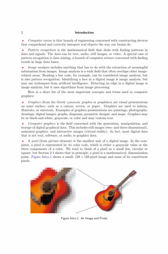
A pixel (from picture element) is the smallest unit of a digital image. In the com-puter, a pixel is represented by its color code, which is either a grayscale value or thethree components of a color. We tend to think of a pixel as a small dot, circular orsquare, but Section 2.1 shows that in principle, a pixel is a mathematical, dimensionlesspoint. Figure Intro.1 shows a small, 128 × 128-pixel image and some of its constituentpixels.

Figure Intro.1: An Image and Pixels.

Introduction 3

Digital image. Such an image is a rectangular array of pixels. Early images hadonly black-and-white or grayscale pixels, and featured low resolutions (only a few dozenpixels per centimeter or per inch). Current images are mostly color, where the colors areselected from huge palettes of millions of colors. Today’s images can have resolutions ofhundreds of pixels per centimeter, more often measured as dpi (dots per inch).

3D (three-dimensional) images. Such an image contains much more informationthan a two-dimensional image. In order to fully view a three-dimensional image, it hasto be rotated or transformed in some way. True viewing devices for such images arerare and expensive (holograms come to mind), so most three-dimensional images areprojected on a two-dimensional display and have to be viewed from different directions.

Computer animation. Much as a film is a sequence of still images, a digital an-imation is a sequence of digital images. An animation is organized in scenes, whereconsecutive images in a scene differ slightly in order to achieve the illusion of smoothmovement.

Vector graphics. Older graphics displays were of this type. In a vector graphicscomputer system, the program running in the computer creates a picture out of graphicscomponents such as points, lines, and circles. A set of such components is stored inmemory and becomes the description of an image. Special hardware translates eachgraphics component in memory into a visible part on the output (normally a display).The total of all the parts on the display constitutes the image.

Raster graphics. Most current graphics displays are of this type. The screen displaysan image that consists of small dots (pixels). The program running in the computercreates an image by assigning color codes to the pixels in memory. The graphics hardwarescans the color codes in memory and actually paints the pixels on the display.

Scan conversion. This is the process of converting a smooth geometric figure intopixels, such that the result looks as smooth as possible. Scan conversion is a verycommon operation, which is why scan conversion algorithms should be fast, using onlylogical operations, shifts, and simple arithmetic operations.

Transformations. Once an image has been generated, the user often transforms it inorder to view different parts of the image or to modify its shape in regular ways. Trans-formations are a must when a three-dimensional image is viewed on a two-dimensionaldisplay.

Projections. A three-dimensional image has to be projected in order to print it orview it on a two-dimensional display. The most common projection is perspective, butparallel projections and nonlinear projections are suitable for special applications.

Rendering is the process of generating a digital image from a mathematical modelby means of algorithms implemented in computer programs. The mathematical modeldescribes the objects that constitute the image in terms of points and curves. Inputsto the rendering algorithm include the orientation of the objects in space, the surfacetextures of the objects (including shading information), and the lighting configuration(the positions, intensities, and colors of the light sources). The term rendering has itsorigins in a painter’s rendering of a scene.

4 Introduction

Modeling. A mathematical model of an object is a collection of points and curves.If the object is three-dimensional, the model also contains surface information. Thefirst step in rendering an object is to display its mathematical model as a wireframe(Section 8.11.2).

Color. An understanding of color is essential for dealing with color images andanimation. Chapter 21 discusses the physical meaning and psychological implications ofcolor, as well as the various color spaces and human vision.

Image compression. Images tend to be large, compared to texts, which is whyimage compression is such an important field of research. Images can be compressedbecause their original (raw) representations are inefficient and feature much redundancy.The various image compression methods remove this redundancy in different ways, andChapters 23 through 25 describe several approaches to image compression, especiallyorthogonal and subband (i.e., wavelet) transforms.

The Graphics Processing Unit (GPU)

Graphics is a computationally intensive application. The task of computing and dis-playing a color, high-resolution image on a large screen involves the following steps: (1)The surfaces that constitute the image have to be computed (as discussed in Part IIIof the book), either as polygonal surfaces or as smooth, curved surfaces that are thenconverted to triangles. (2) Each small triangle has to be rendered by simulating the lightreflected from it (Chapter 17). The software has to know the positions, orientations, andcolors of the light sources, and has to perform intensive computations for each triangle.(3) A texture is sometimes embedded in a surface. The texture is a small bitmap thatis wrapped around the surface to enhance its look. (4) Once rendered, a triangle hasto be projected to two dimensions (see Part II of the book). The projection can beparallel or perspective. (5) When the projection of a triangle has been determined (i.e.,the two-dimensional coordinates of its three vertices are known), its visibility must bedetermined (Chapter 18). A triangle (a small part of a larger surface patch) may becompletely or partially obscured by other surface parts that are closer to the camera(or the observer). Only those parts of the triangle that are visible to the camera shouldparticipate in the next step. (6) Those parts need to be scan converted (Chapter 3).A special algorithm is needed to determine the best pixels for each visible part of thetriangle.

It has therefore been recognized in the early days of computer graphics that thereis a need for special, dedicated hardware to perform most of these operations, which iswhy several companies started developing such hardware as early as the 1970s. The firstunits were special-purpose processors for creating bitmaps of text and simple graphicsshapes and sending them to the video output. The 1980s saw graphics controllers forthe IBM PC and the Commodore Amiga. Those devices tried to accelerate graphics

Introduction 5

operations and implement various two-dimensional graphics primitives in hardware. Inthe case of the Amiga computer, the graphics unit also handled scan conversion of lines,filling of regions, and performed block image transfers.

As hardware manufacturing capabilities improved during the 1990s, more graphicscards, graphics accelerators, and support devices for three-dimensional graphics opera-tions were introduced for both personal computers and console games. In some cases,three-dimensional graphics operations became possible only if an accelerator was in-stalled in the computer. The graphics programming language OpenGL appeared in theearly 1990s and became so popular that users started demanding graphics processorsthat can be programmed in OpenGL.

It was only in the late 1990s that the first GPUs, made by Nvidia (which also coinedthe term GPU) were introduced. These devices (in combination with high-resolution dis-play monitors and drawing and illustration software) have turned our personal computersinto fast, high-resolution graphics generators, and have made it possible for anyone tocreate high-quality original graphics such as maps, plans, drawings, animations, games,and illustrations on a personal computer.

A GPU is a processor mounted on a special graphics card which also includessupport devices, memory, and a bus. The graphics card can be plugged into the computerand later replaced with a more powerful version, but in most current personal computersthe card is simply part of the main circuit board. The main functions of the GPUand its support devices are fast floating-point operations and vector operations. Theseoperations are used all the time in surface computations, rendering, and visible surfacedetermination.

Today (2011), GPUs feature parallel computational units that can perform theiroperations simultaneously. A parallel processor is notoriously difficult to program, whichis why software writing for parallel GPUs is now considered an important field which isdubbed “general-purpose computing on GPU” or GPGPU.

All problems in computer graphics can be solved with a matrix inversion.—James F. Blinn, What’s the Deal with the DCT (1993).

The Fundamental Equation of Computer Graphics

Mathematicians like fundamental theorems. The fundamental theorem of a fieldof mathematics is the theorem considered central to that field. There are fundamentaltheorems of calculus, algebra, arithmetic, vector analysis, Galois theory, Riemanniangeometry, and more.

Theorems and proofs are rare in computer graphics, which is not as rigorous asmathematics. However, there is one equation that appears many times in this book andcan be considered fundamental in computer graphics. This fundamental equation is theexpression for the basic linear interpolation, Equation (9.1)

P(t) = (1 − t)P0 + tP1,

where P0 and P1 can be numbers, points, curves, and even images (as, for example, inSections 2.31.1 and 8.5). It is easy to see that P(0) = P0 and P(1) = P1. In general,

6 Introduction

P(t) is a mixture (or a combination) of (1− t)% of P0 and t% of P1. Notice that thesepercentages add up to 1. When the parameter t is varied from 0 to 1, P(t) varies linearlyfrom P0 to P1. (See the epigram at the end of Chapter 13.)

You know what? I can’t stand introductions. Weird coming from

an author, right? It’s like some committee got together and

said that you’ve got to have an introduction in your book.

Oh, and please make it long. Really long! In fact, make it

so long that it will ensure no one reads introductions.

—Matt Kloskowski, The Complete Guide to Photoshop Layers, 2011.