Computer Science with

Eckart Modrow

Computer Science with

– Snap! by Examples –

© Eckart Modrow 2018 [email protected]

This work is licensed under a Creative Commons Attribution-Noncommercial-Share Alike 4.0 International License. It allows download and redistribution of the complete work with mention of my name, but no editing or commercial use. In addition to the book, the com-plete listings of the described programs are loadable from the following address:

http://emu-online.de/projectsOfCSwithSnap.zip

The scripts are developed with Snap! 4.1.2.1 Build Your Own Blocks.

Prof. Dr. Modrow, Eckart:

Computer Science with Snap!

- Snap! by Examples -

© emu-online Scheden 2018

All rights reserved

If this book is helpful for you and you would like to express your appreciation in form of a donation, you can do so at the following PayPal account:

[email protected] Intended use: Snap! book

This publication and its parts are protected by copyright. Any use in others than legally permitted cases requires the prior written consent of the author.

The software and hardware names used in this book as well as the brand names of the respective companies are generally subject to the protection of goods, trademarks and patents. The product names used are pro-tected by trademark law for the respective copyright holders and cannot be freely used.

This book expresses views and opinions of the author. No guarantee is given for the correct executability of the given sample source texts in this book. I assume no liability or legal responsibility for any damages resulting from the use of the source texts of this book or other incorrect information.

Preface 3

Preface

This book, similar to its predecessor "Informatik mit BYOB"1, uses a collection of program-ming examples to explore the scope of the graphical language Snap!. It does not replace a textbook that conveys CS content but shows how to use Snap! to apply CS methods.

After Scratch and BYOB, Snap! in the current version 4.1.2 is the next step in the devel-opment of graphical tools. The system overcomes several limitations that existed with its predecessors, so it overcomes many arguments against graphical languages. The current version is expanded by numerous extensions in the field of object-oriented programming (OOP). It can meet and exceed all requirements up to high school and beyond. Since drastic improvements have been achieved at the execution speed and availability of libraries in different fields like pixel access, audio or use of external resources, there is hardly any re-striction in applications. Particularly noteworthy in this area is the possibility to use Java-Script functions, e.g. for time-critical operations or extensions within Snap!. The libraries contain numerous JavaScript-examples.

The selection of problems in the following chapters is relatively conservative, partly based on existing computer science lessons, but it goes beyond that. That's intended. I hope, on the one hand, to "pick up" the teaching colleagues from the traditional lessons, and on the other hand, to provide contexts that brings sense from the perspective of a learner to the information to be acquired. In this way, teaching should be very much based on creativity, but also on CS concepts. The examples describe in detail the handling of Snap! in different aspects. After an introductory chapter that gives a fast overview about Snap!, the first few chapters explain the features of the language, followed by sections without direct applica-tion reference. This compromise is due to space requirements, because advanced concepts require extended problems. The examples are not hierarchically ordered, also in the sec-ond part are rather simple ones. At the end of the book there are summaries of the meth-ods used in the examples and an index.

This book is a translation from German. Unfortunately, I do not speak English well, so it will be bumpy. I apologize for that. But all programs have to be changed, hardly anyone else can do this work. Be strong and hold it! Many thanks for the wonderful help of the DeepL2 translation program. I would probably never have finished without these.

I would like to thank Jens Mönig for his support - and for the results of his work. The learn-ers will be thankful!

I wish you a lot of fun working with Snap!.

Göttingen, am 1.4.2018

1 E. Modrow, Informatik mit BYOB, http://ddi-mod.uni-goettingen.de/Informatik%20mit%20BYOB.pdf 2 https://www.deepl.com/translator

Content 4

Content

Preface ……….…………………………………………………………………………………………………….……… 3

Content ……….………………………………………………………………………………….………………………… 4

1 CS and Media Studies …………….…..…………………………………………………………..…..……… 7

2 About Snap! ………….……………………..………………………………………………………….….……… 9 2.1 Block Oriented Languages …………………………………………..……………………………… 9 2.2 Object Oriented Languages ……….………………………………..……………………………… 9 2.3 Inheritance by Delegation ..………..……….……………………………………………………… 10 2.4 What is Snap!? ……...…….………………..…………………………………………………………… 11 2.5 What is Snap! not? ……………………………………………………………………………………… 12 2.6 The Snap!-Screen …………..…………...……………………………………………………………… 13 2.7 An Example for Experienced Users: Flu …………..………………………………….…….... 14 2.7.1 Writing Your Own Methods …….……………………………………………….…….... 15 2.7.2 Elementary Algorithmic and Variables ……….…………………………...…….... 16 2.7.3 Creating Objects …..………………………….……………………………………...…….... 17 2.7.4 Communicating with Objects ……………….…………….……………..…………..... 18 2.7.5 Drawing a Diagram …………….……………………….…….…………………………..... 21

3 Simple Examples …….…..………………………………………………………………………..….………… 23 3.1 Swimming ..……..…………….…………………………………………..………………….…………… 23 2.2 Solar System ………..…………………..………………………………..………………….…………… 25 2.3 Caesar Encryption …..…………..……………………………………..………………….…………… 27 2.4 Tasks …..……………………………….……….…………………………...………………….…………… 29

4 Simulation of a Spring Pendulum ..………………………………………………………..….………… 30 4.1 Organization of Cooperation ..………….………………………..………………….…………… 30 4.2 The Clock …..………..……………………………………………………..………………….…………… 32 4.3 The Exciter …...……………………………….…………………………..………………….…………… 32 4.4 The Thread .………………………………………………………………..………………….…………… 33 4.5 The Ball ……..…………………………………………………...………….………………….…………… 33 4.6 The Pen …..………………………………………….…………...………..………………….…………… 34 4.7 Why is it a simulation? ………………………………….…..……....………………….…………… 34

5 Troubleshooting with Snap! ……………………...……………..…………………………..….………… 35

6 Lists and Related Structures …………..…….…….…………….………………….………..…………… 37 6.1 Selection Sort ………………………..….…….………………………………………………………… 37 6.2 Quicksort …………………………………………………………………………………………………… 39 6.3 Routing with Dijkstra Method …….………………….…….…………………………………… 40 6.4 Matrices and FOR-Loops .………..…..……………………….…………………………………… 44 6.5 Tasks ………………………………..………………….……………….…………………………………… 46

7 Object-Oriented Programming ………….………..…………….…………..…………………………… 47 7.1 Anne and the Filing Cabinets …..………………………………………………………………… 48 7.2 Magnets …..…………………………….……………………………………….………………………… 52 7.3 A Learning Robot …….……………………………………………………….………………..……… 53

Content 5

7.4 A Digital Simulator …..….…………………………………………………………….……………… 57 7.4.1 Sockets and Connections ………..…………………………….………………………… 58 7.4.2 Switches …..…………………………………………….…………….………………………… 59 7.4.3 Gates …..……..………………………………………….…………………….………………… 60 7.4.4 The Pen …..…………….………………………………….………………….………………… 60 7.4.5 LEDs …..…………….……………………………………….…………………….……………… 61 7.4.6 The Interaction oft the Components ….……….…….……………….…………… 61 7.4.7 Tasks …..……………….…………………………………………………………….…………… 62

8 Graphics …………..………………..……………………………………….……………………………………… 63 8.1 Line Graphics ………………………………..…………………………………………………………… 63 8.2 Pixel Graphics and RGB Model .…………….…………………………………………………… 66 8.2.1 Pixel Graphics with the Pixels Library …………………..…..……..……………… 66 8.2.2 Pixel Graphics with an own Library ………………..….…..……………....……… 68 8.3 The Light of the old Stars ….……………….……………………………………………………… 70 8.4 A simple RGB Color Mixer ………….……………….….…….…………………………………… 71 8.5 Drip Painting …………….………………………………………….…………………………………… 72 8.6 Edge Detection ……….…………….……….…………………….…………………………………… 74 8.7 Tasks …………………..…….………………………………………….…………………………………… 76

9 Image Recognition …….…..……………………………………………………………………..….………… 77 9.1 A Barcode Scanner ..……..……….…………………………………..…………….………………… 77 9.2 Project: Transit Prohibited! ….…………………..………………..…………….………………… 82 9.3 Project: Face Recognition …..……….……………………………..…………….………………… 88 9.4 Tasks …..………….………………………….……………………………..…………….……….………… 94

10 Sounds …….………………..………………………………..………..………………………………….………… 95 10.1 Find Sounds ..……..……………………………………………………………………………….……… 95 10.2 Processing Sounds..……....……………………………………………………………..……..……… 96 10.3 Making Music ..……..…………………………..……….…………………………………………….… 97 10.4 Project: Hearing check ..……..………………………………….……………….…………..……… 99 10.5 Tasks ..……..…….….…………………………………………………………………………….….……… 100

11 Project: Electrons in Fields …………..………………..………………………………..……….………… 101 11.1 Electron Source and Set-Up ..………………………………....…………………………..……… 101 11.2 Capacitor and Electric Field …..………………………….……..………..…….………………… 102 11.3 Helmholtz Coils and Magnetic Field …..…………………………….……….………………… 103 11.4 The Electrons …..………………………….……………………………..…………….………………… 104

12 Texts and Related Topics ………….………………..…………………………………………….………… 106 12.1 Operations on Strings ……………………..…………………………..……………………………… 106 12.2 Vigenére Encryption …………………………………………………………………………………… 109 12.3 DNA-Sequencing ………………..…………….………………………………………………………… 111 12.4 Text Files and Frequency Analysis ...…………….……………………………………………… 113 12.5 SQL-Databases ...…………………………………………………………………………….……………117 12.6 Tasks ………………….…………………………....………………………………………………………… 123

Content 6

13 Computer Algebra: Functional Programming ……..……………………………….……………… 124 13.1 Function Terms ……….…………………………………………………..………………………………124 13.2 Parsing of Function Terms …………………………………………..……………………………… 125 13.3 Derivation of Function Terms ..…….……………………………..……………………………… 129 13.4 Calculation of Function Results and Graphs ……………………..………………………… 131 13.5 Tasks ………………….……………………………………………………..…………………..…………… 134

14 Artificial Plants: L-Systems …………………….…………………………………………….……………… 135 14.1 L-Systems …………………….……………………………………………..……………………………… 135 14.2 Create the Drawing Instruction ..…..…………………………..……..………………………… 136 14.3 The Stack Operations …...…..………………………………………..……………………………… 136 14.4 Drawing the Plants ……………...…………………………………………………..………………… 137 14.5 Tasks ………………….……………………………………………………..……………..………………… 138

15 Automata ……..……………….…………………………………….…………………………….……….……… 139 15.1 Correct Mail Addresses ………..……………………………………..……………………………… 139 15.2 Hyphenation: Kevin Speaks ……....……………………………..……..…………………….…… 141 15.3 Coupled Turing Machines ….........………………………………..……………………………… 145 15.4 Cellular Automata: Iterated prisoner’s dilemma ………………….……………………… 149 15.5 Tasks ………….……….……………………………………………………………………………………… 155

16 Projects ………….………………..……………………….……………….…………….………………………… 156 16.1 LOGO for the Poor ………………………..…………………………………………………………… 156 16.2 SnapMinder by Jens Mönig …..…………………………………………………………………… 163 16.2.1 Importing Table Data ………………….…………..……..………………….………… 164 16.2.2 The SnapMinder Data ..………………….…..……..…………………………….…… 165 16.2.3 The SnapMinder Countries …………….…..……..………………………………… 167 16.2.4 Use SnapMinder ……….………………….…..……..………………………..………… 168 16.3 Connectivity: The World is Small .……………………………………………………………… 169 16.3.1 Random Networks ………………….…..……..………………………………………… 170 16.3.2 Scalefree Networks ………………….…..……..…………………………….………… 171 16.3.3 The Implementation .………………….…..……..……………………………….…… 172 16.4 Evolution …..……………………………………………………….………………………………………176 16.5 Using the Sensorboard Calliope …..……….…………………………………………………… 180 16.6 Rate Websites: PageRank ……………..…………………………………………………………… 182

17 At the Supermarket …….…………………………….……………….…………………………………….… 188 17.1 Warehouse Management with SQLite …..…………………….………………….………… 189 17.2 The Scanning Cash Register …………………….…..………….………………………………… 192 17.3 The Smart Scale …………………….…..………………..……………………………………….…… 194 17.4 License Plate Recognition ….…….………………….…..………………..……………………… 200 17.5 The Advertising Department ….………………………………..…..…………………………… 206

About the Notation of Snap!-Programs …………….………………………………………………….…… 208

How to … ? ……………………………….….……………….…………………………………………………..……… 210

Index ……………………….……………….………………………………………………..……………………..……… 212

1 CS and Media Studies 7

1 CS and Media Studies

In schools and universities, there is a lot of discussion about media literacy as part of the "digitization offensive". Since the term "digitization" obviously concerns computer science, CS should participate in the discussion. Educational institutions need to think carefully about their contribution to a comprehensive education. On the one hand, children and adolescents also gain knowledge and experience - and in many areas predominantly - out-side of these institutions; on the other hand, the objectives of "education" and " vocational training" should be sharply differentiated. Adolescents do not necessarily have to master the handling of current tools, they can confidently leave that to the adult. But they must be prepared to take on the appropriate role with future tools.

It is often argued that learners must learn to use modern media to lose the "fear of them". I think that is wrong. First, children and adolescents usually are not afraid of the media, but they are curious about them. Second, they learn to handle media quickly and easily by others and by use. The fear is more on the side of the elderly, who did not grow up with this technique and therefore feel insecure with it. Older people should remember that in their youth, the elderly at that time discussed how to approach the handling of mouse-controlled surfaces to relieve them of fear. We can learn from this situation that the han-dling of current technology, such as smartphones, can be acquired by the way, but obvi-ously this does not lead automatically to an uncomplicated use of future technology.

Goal 1: Learners need to be empowered to understand the basics of future technologies and to acquire their use.

Media usage is not the same as media consumption. The passive use of media of whatever kind, e.g. simple "gawking", cannot be the goal of the education system. When we engage with media, they must be in a context that activates learners.

Goal 2: Learners need to be empowered to select and deploy tools to create media based on their problem. So, they first must learn how to solve problems independently.

Independent problem solving usually is not seen as a central task, at least in schools. Cre-ative subjects such as art, music and (hopefully) some of the languages at least sometimes strive for this. Mostly well-behaved learning is in the foreground. But CS provides tools to realize and test one's own ideas even in relatively rudimentary form. Not to realize creative lessons would be a missed chance. However, this will only work if the teachers themselves have experiences in independent, creative problem-solving, and if they trust in the learners accordingly. If the teachers themselves only have "well-behaved learned" CS content, then creativity in the classroom will usually not work out. If the second goal is to be realized in schools, this should and must also have consequences for teacher training at universities.

Goal 3: Teachers need to be empowered to plan and realize creative lessons. There should be opportunity and time in their own studies.

Modern media such as social networks have profoundly changed social life, communica-tion, etc. The consequences are hard to predict while this process is still going on. Much less they could be seen before it was started. I think it would be a complete overstrain of teachers to demand that they address the actual social consequences of computer science systems in the classroom, which include the impact of digital media. That would not be

1 CS and Media Studies 8

expedient, because the view on “what has happened” necessarily is turned backwards. But what you can ask for is to show that the use of computer systems has social consequences and that these depend very much on how the systems are designed. Different problem solutions have different consequences - and vice versa: If certain consequences are unde-sirable, then it will usually be possible to find another technical problem solution.

Goal 4: Learners need to know that there are almost always different solutions to prob-lems. You should think about their effects, which of course are not conclusive. They learn that these effects are not given but can be shaped.

Why does this affect Snap!?

Graphical programming tools like Snap! do not only contain the algorithmic components, but are embedded in a media environment, which does not only allow the use of graphics, sound, ... but requires it. When a problem is handled, cameras and graphics programs can and should be used to create the appropriate costumes and costume changes that visualize the current state of the system. Sound programs make it possible to comment on the course itself, to edit and insert music or to design it yourself. And, of course, the results must be presented because product pride is an important motive for the dedicated work. And there is much interest in the results of others. Snap! allows algorithmic problem solv-ing at a very high level, but it not only allows the analytical approach, but also the playful, the experimental, the creative, ... Not allowed is passivity, because nothing happens by itself. Media are essential system components, e. g. to visualize the results - and they can also be the result itself. Snap! therefore offers the opportunity to model problem solutions for current problems, also and especially in the field of media. The self-created algorithmic framework of the model creates understanding of the observed processes in real life. The experience of being able to gain this insight enables active, critical analysis of future tech-nology. The examples in this book are intended to show that this is possible in many areas

using elementary methods. They should encourage you to get started yourself. 😉

2 About Snap! 9

2 About Snap!

2.1 Block Oriented Languages

Snap! 3 is a successor of BYOB (Build Your Own Blocks), whose name already describes part of the program: the users at schools and universities use existing commands in the form of blocks and are enabled to develop own new blocks. Their programs (scripts) are combinations of both. You must know that almost all programming languages are block-oriented: command sequences can be grouped with a new name. The resulting new com-mands can use values (parameters) to work with, if needed, and they can return results. This gives us several advantages:

Programs become shorter because program parts are swapped out into the blocks. Multiply used command sequences are written only once and then reused under the new name.

Programs contain fewer errors because blocks are developed and tested largely inde-pendent. The developed command sequence thus remains short and clear. "Long" pro-gram parts are rarely necessary and usually a sign of poor programming style.

Programs get their own style because the new commands reflect the way a program-mer solves problems.

The programming language is extended because the created blocks represent new commands and thus new possibilities.

2.2 Object Oriented Languages

When dealing with more extensive problems, the number of subproblems to be solved increases. Often these can be combined to groups which can be assigned to concrete ob-jects. Often, these sub-problems appear time and again, so they can be solved when ap-propriate objects are provided, e. g. in libraries. An important aspect of this way of working is that it allows teamwork to be carried out well, with the different teams creating objects that solve part tasks. Of course, the results must be put together. The object-oriented ap-proach is often realized by creating classes that describe the behavior of a group of similar objects. From these classes instances are created that are supposed to solve the problems. In contrast Snap! realizes a prototype-based approach. For each object an example, the prototype, is generated and tested step by step. If one is satisfied with the result, further objects of this kind are derived by duplication (cloning) of the prototype. This way is better for beginners.

The object-oriented approach has following advantages:

Problems become understandable because sub-problems can be assigned to objects and (largely) solved independently. Problems become clearer because the division into objects often corresponds to the intu-itive view, so that "everyday knowledge" can be incorporated into the solutions.

3 http://snap.berkeley.edu/snapsource/snap.html

Advantages of block-oriented languages

Advantages of object-oriented languages

2.2 Object Oriented Languages 10

Problem-adapted tools can be provided because corresponding libraries exist or are cre-ated. Collaboration is facilitated because object-oriented work suggests the broader isolation of problem solving so that the different groups are less disturbed.

2.3 Inheritance by Delegation

The concept of inheritance is central to object-oriented programming. It can be realized by classes or by delegation. In the original article by Lieberman4, who describes the prototype-oriented approach to delegation very early, objects are understood as the embodiment of the concepts of their class. For example, the elephant Clyde stands for everything the observer knows about an elephant. If he imagines an elephant, there appears no abstract class of elephants, but just Clyde. When he talks about another elephant, here: Fred, he describes it like this: "Fred is like Clyde, just white."

What does this approach mean for the learning process? If the learner only knows one copy of a class (here: Clyde), the prototype completely describes his knowledge, an ab-straction is pointless for him. If he later learns about other specimens and describes them through modifications to the original, thus replacing some methods with others, changing attributes and adding new ones, then slowly the image of the class itself emerges as an intersection of the common properties. Now the process of abstraction is comprehensible for him and after a few attempts also feasible. Delegation thus is a process that maps the learning process itself by creating prototypes instead of classes.

In Snap! we mainly work according to this principle, which is presented below in detail. If you really want, a class system also can be implemented.

In Snap! sprites are created as prototypes and equipped with the desired attributes and methods. If their behavior has been sufficiently tested, clones can be generated dynami-cally using the clone block. Each sprite has a parent (may be null) and children (also may be null). The parent property can be set and / or modified later, so the system of depend-encies is dynamic. If the program stops, all dynamically generated clones are deleted, which is beneficial.

At first, a clone inherits (almost) all the attributes and methods of the mother object. This is indicated by a "paler" representation in the palettes. If a sprite overrides inherited at-tributes or methods, they replace those of the prototype, as usual. If you delete the over-rides again, then the inherited appear.

4 Lieberman, Henry: Using Prototypical Objects to Implement Shared Behavior in Object Ori-ented Systems, 1986, http://web.media.mit.edu/~lieber/Lieberary/OOP/Delegation/Delegation.html

cloning sprites

2 About Snap! 11

2.4 What is Snap!?

Snap! was (and is) developed by Brian Harvey and Jens Mönig for the project Beauty and Joy of Computing5 and is made freely available on the internet. Since the system runs in the browser, it does not require any installation and works on almost all devices6. It is sim-ilar in surface and behavior to Scratch7, a free programming environment for children de-veloped at MIT8. However, the implemented concepts go far beyond this: here are the roots at Scheme, a LISP language, teaching language for decades at MIT. They are intro-duced e. g. in a famous textbook by Harold Abelson and Gerald and Julie Sussman9. Snap! is thus a fully developed programming language that can be used for (almost) all problems. For most, it is sufficiently fast now. That is not self-evident and was a shortcoming of their predecessors. Graphical languages are largely concerned with controlling the state of the system. For example, to allow you to interrupt endless loops or to "tolerate" access errors to data structures. There remains little time for program execution.

Snap! is a graphical programming language: programs (scripts) are not entered as text but composed of tiles. Since these tiles can only be joined together if this makes sense, "mis-spelled" programs are largely prevented. Snap! therefore is largely syntax-free. Neverthe-less, it is not entirely free of syntax, because some blocks can handle different combina-tions of inputs: if you combine them incorrectly, errors can occur. However, this happens more in advanced concepts. If you apply these, you should know what you are doing.

Snap! is extremely "peaceful": mistakes do not lead to program crashes but are indicated by the appearance of a red marker around the tiles that caused the error - without dra-matic consequences. The used tiles, which include the newly developed blocks, always "live". They can be executed by mouse clicks so that their effect is directly observable. This makes it easy to experiment with the scripts. They can be tested, changed, broken down into parts and put together the same or different. This gives us a second access to pro-gramming: in addition to problem analysis and the associated top-down approach, the ex-perimental bottom-up construction of subprograms, which can be put together to form a complete solution.

Snap! is clear: both program sequences and assignments of the variables can be displayed and tracked on demand on the screen.

Snap! is extensible: with the implemented LISP concepts, new control structures can be created, e. g. to work with special data structures.

Snap! is object-oriented, even in different ways: Objects can be generated by creating prototypes with subsequent delegation, as well as in different ways by classes.

Snap! is first-class: all structures used are first-class, so they can be assigned to variables or used as parameters in blocks, can be the result of a function block or content of a data

5 https://bjc.berkeley.edu/ 6 These are, of course, computers, tablets, smartphones, ... 7 http://scratch.mit.edu/ 8 Massachusetts Institute of Technology, Boston 9 Abelson, Sussman: Struktur und Interpretation von Computerprogrammen, Springer 2001

the developers

origins at Lisp

barely syntax errors

two styles of programming

vivid and expandable

object-oriented

2.4 What is Snap! 12

structure. Furthermore, they may be untitled (anonymous), which is important for the im-plemented aspects of the lambda calculus, the basis of LISP. Consequently, the logo of Snap! contains the same proud Lambda, which builds the hair of Alonzo, the mascot of BYOB.

2.5 What is Snap! not?

Snap! is not a tool for professional software production. It started as a technology study commissioned by the American Ministry of Education under CE21 (Computing Education for the 21st Century), which is also designed to reduce the drop-out rate in technical sub-jects. It is a tool to implement and test CS concepts by way of example.

Snap! primarily is used for work in the field of algorithms and data structures. Due to the browser environment, essential areas of computer science such as access to files or hard-ware can be embedded via extensions but are not (yet) part of the core language. How-ever, the built-in url-block allows in the meantime quite easy access to the Internet and thus using intermediary servers to databases or external hardware. Both are included in the book.

Since the code of Snap! is freely available, there are different modifications. Whether that is a curse or a blessing, it will be shown.

the limits

Alonzo

2 About Snap! 13

2.6 The Snap!-Screen

The Snap!-Screen consists of six sections below the menu bar 10.

On the far left are the command tabs, divided into the categories Motion, Looks, Sound and so on. If you click on the corresponding button, the tiles of this category are displayed below. If they don’t fit all on the screen, you can scroll the screen area in the usual way.

To the right, in the middle of the screen, the name of the object currently being edited as well as some of its properties are displayed. The default name of the sprite can - and should - be changed here.

Underneath is an area in which, depending on the tab, the scripts, costumes and sounds of the sprite can be edited or created.

Top right is the output window where the sprites move. This can be resized using the buttons above or via the entry in the tool menu (Stage size ...).

Downright the sprite corral displays the available sprites. If you click on one, the middle section changes to its scripts, costumes or sounds - depending on the selection.

The menu bar on the left offers the usual menus for loading and saving the project as well as individual sprites. Furthermore, many settings can be made. One possibility is to set the language. Nevertheless, I recommend that you stay with the English version, as it is possible to differentiate your own blocks, titled e. g. in German, from the native ones at first glance.

On the far right we find the green flag known from Scratch, with which several scripts can be started at the same time when using the corresponding block. The pause button next to it pauses everything accordingly and the red button stops all running scripts. Individual scripts or tiles can be started simply by clicking on them.

10 The division of the areas can be changed with .

Sprite-bezogene Einstellungen

the menu bar

the tool menu

2.7 An Example for experienced Users: Flu 14

2.7 An Example for Experienced Users: Flu

The example simulates the spread of a flu epidemic under different conditions. It provides a quick overview of the essential features of Snap! and is intended especially for experi-enced programmers. Beginners should read the next chapters first.

The question is which proportion and which special groups of people in a population should be vaccinated if the spread of a flu epidemic is to be stopped. The question is not so easy to answer, because the outcome depends on several parameters: the likelihood of infec-tion indicates how probable the infection of a healthy person in contact with a sick person is, the seroconversion time is the time between infection and immunization, the numbers of healthy and diseased persons at the beginning of the simulation determines the number of contacts between them, and the number of multipliers indicates how many people in the population have particularly large numbers of contacts or contacts to particularly dis-tant groups. If one of them becomes infected, e. g. the disease will be worn in distant areas. Since contacts, infections, … are randomized, we will only achieve sustainable results if we perform the simulation multiple times with the same parameter values - and after that we still must discuss which values represent "results" in the sense mentioned. That's why the topic is perfect for a small classroom project. A "control group" develops the higher-level scripts, in this case assigned to the stage. It designs the task distribution with the other two groups. The other groups develop the prototypes person and graph, which are largely independent of each other.

three prototypes for three groups

2 About Snap! 15

2.7.1 Writing Your Own Methods

At various points it is necessary to get rid of the clones of a prototype without exiting the program. We achieve that by a new method delete all clones of <prototype>. It is a Command block, which is a command with (in this case) one parameter. (Function blocks are called Reporter in Snap!.) New blocks are written in the block editor. It can be started with the buttons Make a block we find in the palettes or – the fastest way – by right-clicking on the script layer and calling it from the context menu. First, we specify the method name, if desired with blanks and special characters, select the type (Command, Reporter, or Predicate) and indicate whether it’s a global ("for all sprites") or local ("for this sprite only") method. We can also choose the palette to which the block is to be included. I do not recommend this: The best place to find the gray self-written blocks is the bottom of the Variables palette. For example, if you evaluate student programs, it is often a problem to find the newly created blocks at all.

After pressing the return key, the Block editor opens, and the block name appears – with + characters in the spaces and margins. There, we can open another menu by mouse clicks, which allows to insert parameters in these places and to assign types to them if necessary. In our case, we click on the far right, enter the parameter identifier prototype and click the small right arrow to specify the typing. After that a selection box opens11. We choose as type Object (the arrow), come back into the Block editor, and drag the required commands into its script area.

Our method uses two script variables (clones and thisClone) known only in this block. It asks the parameter prototype, which later is passed with a ref-erence to the prototype of all persons, for its descendants – these are all occurring dynamically generated "persons"12. As long as these are still avail-able, it will store the first in one of the script variables, delete them from the list, and then ask that person to delete themselves, with tell <thisClone> to <delete this clone>13.

11 This box is described in detail in the snap-reference manual that you get when you click the Snap! icon on the top-left of the window. 12 The clones created statically through the context menu in the sprite area are not found there. 13 The delete block can only be found in the palettes of the sprites. You can reach it in the stage via the search function at the top of the palette area.


2.7.2 Elementary Algorithmic and Variables

To define the parameters and other control values, we use the stage, which we click in the sprite corral. This responds to the message "go" by setting the initial parameters and de-termining which quantities are to be measured in the simulations. Thereafter, correspond-ing simulation runs are started.

In detail: Since initially only the prototype person is available, we "fish" for him using the block my <other sprites> from the Sensing palette. The prototype is the first element of the received list. We store it in the global ("for all Sprites") variable prototype person that we created previously in the Variables palette. We also created all the other required variables via the Make a variable button, with the ones needed only within the stage being marked as local ("for this sprite only"). You can recognize them at the "marker" be-fore the name. The others are global. Global variables are displayed at the top of the Var-

iables palette, then follow the local ones. The output area is cleared (there might be an old graphic), some variables get appropriate initial values and a list called data to record the simulation results will be deleted (set <data> to <list>). This part could have been well outsourced to a separate block, but since we want to experiment with the variable values, it is better if they are "on the table".

In the following, the number of initially vac-cinated (the immune

normal) is increased from zero to 100 in steps. We find the con-trol structures for this in the Control palette. For each value, a series of simulation runs is performed, and the mean value is deter-mined from the results (here: the maximum number of infected). The variable number

of simulations deter-mines how often this happens. After each run, the results are en-tered as a percentage in the data list. Finally, the Graph sprite will be asked to create a graphic.

2 About Snap! 17

2.7.3 Creating Objects

In addition to the script already described, the control program uses another one: simulate. In it, some initial values are reset, and the corresponding number of per-sons are generated, which differ in type (normal, multi-

plier) and status (healthy, infected, immune). After that the simulation run is started by sending the message "come on!" which is heard by all objects in the system.

How to create objects?

In the method we create a person type: <type> and

status: <status>. A local script variable p references a newly created clone of the specified prototype. After that, the clone is present, visible and accessible under the name p – quite simple.

However, the clones should differ in type and status. For this, they contain (here) a local method inherited from the prototype setup <status> <typ>. We have to call these with the given parameter values. We therefore "tell" the object p that it should execute this method. As this is local to persons, we take the <attribute> of <ob-

ject> Block from the Sensing palette, select the proto-type in the right-hand box (here: Person) and after that in the left box the desired method (here: setup). Because two parameters are to be specified, we expand the block with the small arrow keys and enter status and type be-hind with inputs. The block is to be understood as "p, please execute in your context of methods and variables the method passed with the specified parameters". The block is equivalent to the well-known dot notation of the OOP languages: p.setup(status,type);

invoked methods in Person


2.7.4 Communicating with Objects

We are now coming to the actual players in our flu project: the persons. These are symbol-ized by small circles whose color expresses their status. "Normal" persons scurry around relatively small-step in their environment and meet the neighbors, where they can be in-fected or can infect. After a certain period, the seroconversion time, they become immune and do no longer infect, are no longer infected. Vaccinated persons are immune from the beginning. Some of the people are "multipliers", i.e. they jump quite wildly around the area and can spread the infection quickly. They are color coded like the normal, but slightly different. We produce appropriate costumes in the graphic editor or a drawing program and import them into the Costumes section.

Once the persons are created, they all receive all the message "come on! ". They respond to this message because they have a hat-block from the control palette that responds to "come on! ". After that, they get into an infinite loop that only breaks when the global variable finished? gets the value true. This is the case when there are no more infected.

In this loop, the following actions are performed repeatedly:

1. Objects are searched near the person and stored in the list neighbors. Too far objects are deleted in this list.

2. Any remaining neighbors may become infected or infect the person if they are ill. 3. It is checked whether the person has to be immune, if the Seroconversion time has

expired. The corresponding variables are changed. 4. After that, the person moves according to their type.

Since data has to be exchanged between persons during these processes and other peo-ple's method calls are initiated, the example shows a few ways to do this:

The ask <object> for <function call> block is used in the script when looking for neigh-bors. Because the members of the neighbors list can be arbitrary objects, we throw all non-person objects out of the lists. In this case, this can only be a Graph sprite. We use the my <attribut> block from the Sensing palette to ask each object for its name: ask

<item <i >> of <neighbors> for <my <name >>. A little further down, this is done again in the status query. Again, the <attribute> of <object> Block is executed in the context of the other object. Therefore, the blocks are surrounded by a gray ring indicating that the unevaluated code of the block is passed and not its current result.

Directly above, the same happens to the local command infect. This is done - as already described - via the tell block.

2 About Snap! 19

In two places below, local methods - shown in gray - are executed in the context of the object. This happens "normally" when the block is reached.

Blocks for direct communication be-tween objects


The method infect infects the current object, if necessary, and changes the appropriate numbers. After that the appearance of the object is changed.

The method show yourself select the appropriate costume and determine if there are still infected people left.

2 About Snap! 21

2.7.5 Drawing a Diagram

Finally, we want to have our results displayed in a diagram. The initial number of vaccinated (in %) and the maximum number of infected persons (in %) were measured. We cre-ate an object for this purpose, which we donate a beautiful pen as a costume. We first have to paint and label a coordinate system on the screen. We find the blocks for this in the Pen-palette and (the label block) in the Tools-Li-brary.

The ascertained data are in list form as variable data:

With the helper method and these data the graph can be created: We send the pen to the first data point, given by a list with the two mentioned entries. After that we lead him lowered to the remaining points - with some re-calculation.

the pen


The result can be admired on the output area:

In each case, 300 "persons" were used without multipliers and with only one initially in-fected (red: infected, yellow: immune, green: healthy). One can see: if half of the popula-tion is to remain healthy in this model, then 20% have to be vaccinated.

blocks of the Pen palette

3 Simple Examples 23

3 Simple Examples

The following examples demonstrate some aspects of Snap!. They are quick to implement and should inspire modifications and extensions. Above all, they show how easy is visuali-zation in Snap!.

3.1 Swimming

Contents: duplicated objects communication via messages local and global variables

We draw a swimmer in three states of swimming (arms elongated or spread, legs bent). These three images additional are mirrored so that the swimmer seems to swim in the opposite direction. Afterwards we draw a swimming pool with pathways as a stage background and look for a costume for a trainer in the costumes library of Snap!. That’s Cassy in this case.

We create two sprites, the first being the swimmer and the second the trainer. If we click on the green flag, the competition should start. The swimmer goes into starting position on the left lane (x = -195). Its x-position is stored in a local vari-able x, which is different for each swimmer. Everyone swims in his orbit. Since the swimmer is a bit big, we scale him to 40%. He then waits for the start signal.

The trainer is also slightly downsized and is sent down-right to the edge of the pool. There she gives a tip to start the competition. She waits for it too.

Since the blue water is part of the stage, it only receives a single script that re-sponds to a mouse click. The stage then sends the message "come on!" only to the trainer. If one uses a two-element list as a message, the first element repre-sents the message, the second the one or more addresses.

After that our trainer sends the message "start" to all, notes that the competition has begun, and then jumps around a bit.

3.1 Swimming 24

Our swimmer starts with the message "start". He notes his start time in a local variable, because afterwards each swim-mer measures his own time. Thereafter, he periodically changes his costume depending on the direction of the swim and glides a random piece forward a random time. His direc-

tion is also stored locally, as the swimmers turn around at dif-ferent times. After the movement, the swimmer shows his new time, measured from the starting time, and checks to see if he should turn back. Then he checks if he is at the finish. If the competition is still running, he is happy because he is the winner. This is indicated by changing the variable competition

is running and sending out a message. It was created as global, since it applies to all participants. In any case, the movement ends at the finish (stop <this script>).

If all goes well, then four duplicates of the swimmer are created by right-clicking on its costume in the sprite area and selecting "duplicate" from the context menu. The lanes of the now five swimmers are assigned by specify-ing the x-value. The time variables of the individ-ual swimmers should be displayed above the tracks. For this purpose, the check mark in the selection box is set in the Var-

iables palette. By right-clicking on the variable display (the monitor) you can choose different representations. We take "large" and slide the ads across the lanes.

If someone has won, the trainer comments on this by setting a script variable of the script to a random value and expressing herself accordingly. That's when her pranc-ing ends.


3.2 Solar System14

Contents: multiple objects parameters and their typing parallel methods

We get a picture of the sun and some planetary im-ages from the net and shrink them a lot. Then we'll load them as costumes into a planet prototype sprite called Planet. A second sprite called Starter organizes the "creation" of a solar system.

Our planet has a set of local variables describing its state. These includes its mass m, the speed components vx and vy, the acceleration components ax and ay as well as its dis-tance from the sun r. These values are passed to it by a global method setup. We create it using the Make a block Button and enter its name. Since the method is to be global, we take the default "for all sprites". Parameters now can be entered for the + characters that appear in the block header next to and between the identifiers. We click the first "+" to the right of setup and enter the parameter name x. We could leave it at that, because Snap! guesses the type of a value (usually) correctly. But we want to typify the parameters. To do this, click on the small right arrow to the right of Input name. An extensive selection window appears. In this we click Number to specify that only numbers can be entered as a parameter value. For the next parameters we proceed accordingly with the name typed as Text. We get:

As a script of this block we now need to insert code that will send our planet to the right place, take the parameter values into the variables, and select the right costume that re-sults from the planet name. Finally, a local method move yourself is started. Because it contains an infinite loop, the program must not "hang" in this loop. Therefore, we start move yourself using the launch block which creates a parallel process (a new thread) and executes it. This allows the program to continue without waiting for an end of move your-

self. Each planet runs in its own thread.

14 In a fairly simplified version: The sun stands like nailed in the middle and the planets do not affect each other.

start parallel processes

3.2 Solar System 26

If the sun is in the origin of the coordinate system, then you

get the gravitational force on the planet 𝑭 = −𝐺 ∗∗ *r

(vectors bold), therefore 𝒂 = −𝐺 ∗ *r. From the two ac-

celeration components ax und ay we calculate changes of the speed components vx und vy and from these changes of the position. This happens again and again in the method move yourself.

Now we have to create an new solar system. We clone our planet three times and baptize the clones Earth, Jupiter, and Saturn. This is done using the context menu in the sprite area.

Finally, our Starter Sprite comes into play. This stamps a sun image in the center of the coordinate system and starts the three planets by calls to the setup method, which works in the context of the planets with their local values.

All values have been selected so that the trajectory curves at least partially fit on the screen.


3.3 Caesar Encryption

Contents: dealing with character strings simple typecasting blocks as macros text output with the tools library event handling

We want to encrypt and decrypt simple strings using the Caesar method. Since this is very hard computer science, we also need a very serious, somewhat boring surface. There should be some buttons on it. We import them from the Costumes library using the File menu. (As you can see, there are much more "interesting" costumes in the library!) The button image is exported to a file. With the help of a graphics program we make it a little bit longer and label it differently. We reimport the resulting costumes. We create three new empty blocks called text input, encryption and decryption and make sure that our buttons respond correct when you click on one of them.

We copy the button twice using the context menu in the sprite area and change the costumes and blocks accordingly. We drag the buttons to the right place, change their names e. g. to bTextinput, and remove the check mark in front of the box draggable. Now the button is stuck.

Then we create four global variables named original text, ci-

phertext, decrypted text, and key. We show them on the screen with monitors (set a tick in front of the variable names) and change to a large representation using the con-text menus in the display area. After that we pull them to suitable places.

We import the Tools library (see above). Here we need only the block label <text> of size <size> from the Pen palette to label the output. To do this, we create a new sprite named Control that provides a very serious interface and changes the variable key when the appropriate key is pressed.

We now come to the actual functionality, which can be developed independently of each other. Text input is simple: we ask for the original text. Sure, the output can be made much more beautiful.

to "nail a sprite"

3.3 Caesar Encryption 28

Caesar encryption consists of moving all characters in the code (here: in Unicode) by the key length. The last characters are moved for-ward cyclically. In the ad-joining script this is done very verbosely, but - hope-fully - legibly. Note that the green length of <string>-block from the Operators palette works with strings, the brown length of <list>-version from the Variables palette works with lists.

The decryption is done inversely for encryption.


3.4 Tasks

1. a: Find out about the XOR encryption. Implement the procedure.

b: Find out about transfer procedures for encryption. Implement the procedure.

c: Find out about the cryptanalysis. Implement a frequency analysis. 2. In the camel problem, the animal is in a terrible situation between three pyr-

amids. It moves purposefully towards a randomly selected pyramid. Once it has travelled exactly half the distance to the pyramid, a hateful desert spirit comes and whirls the poor creature around, so that it no longer knows which pyramid it was driving. The movement, of course, leaves a print on the screen, and the procedure begins anew.

3. The goat problem is popping up in the media every once in a while. The point

is this: in a raffle there are three doors behind which there is a goat in two, behind the third is the main prize. The game leader who knows the positions asks the player to guess a door. He then opens one of the remaining doors, behind which a goat is located, and offers the player to change one's choice – or not. The question is: Should he do that? Realize the game and decide the question empirically.

4. a: Desert ants live alone in the desert. If they leave their burrow they look for

something edible in the area. Once they find this, they run right back to the burrow. Obviously, they remember what movements they have made. From these they calculate the direct way back. Realize the process.

b: On their way to the burrow, the ants lay a pheromone trail that evaporates slowly. On it they find their prey, take another piece and run back to the bur-row, laying a new pheromone track. If they haven't found anything, they won't leave a new trail.

5. Two young ladies sit in the theatre bistro and get bored. One stands up and

goes ... and then the story goes off! But how?

What's your guess?

4.1 Organisation of Cooperation 30

4 Simulation of a Spring Pendulum

In addition to the extensive freedom of syntax, the excellent visualization possibilities and the good-natured behavior of Snap! in case of errors are an incentive for the learners to proceed experimentally and test their own ideas. In addition to the analytical top-down procedure, this results in a bottom-up approach of the trial-and-error, which is important for beginning programmers because it allows them to gain experience in this field, which they can systematize later on. Experimental approach opens up opportunities for inde-pendent problem solving right at the beginning instead of following given results.

In the field of simulations, including many of the usual games, we find enough simple but not trivial problems which can be solved by beginners with a bit of good will. Experimental work naturally requires an interest in developing one's own ideas. We therefore need problems that generate sufficient motivation. As an example, we choose the simulation of a simple spring pendulum, which hangs on a periodically oscillating exciter. Ok, ok, I already know that an example from physics does not have a very motivating effect on all learners - rather in contrary. But I'm not giving up my hope!

4.1 Organization of Cooperation

If groups work largely independently of each other, it must be clear on the one hand in which framework they work, and on the other hand how the results can be brought to-gether later on.

To create a frame, you can create empty blocks with the correct names as "dummies". These can be used in scripts without any functionality. The required objects can also be created and provided with rudimentary behavior, e. g. in response to events: You can, for example, output a speech bubble with an explanatory text: "This and that should actually happen now! " This program frame can be exported and imported as a whole or in parts:

The project can be exported with all its parts using the file menu. It will appear at the bottom of the Snap! window. Clicking on the arrow to the right of it will take you to the download folder where it was saved. From there it can be dragged into any Snap! window and opened again.

If there are global methods (blocks "for all sprites") in the project, another item "Export blocks..." appears in the same menu. If it was chosen, the blocks to be exported can be selected in the window that appears. These can be dragged into open Snap! windows like projects.

4 Simulation of a Spring Pendulum 31

Sprites can be exported with their local methods as a whole by selecting the item "ex-port..." in their context menu in the sprite area. The re-import is carried out as de-scribed above.

Within a project, scripts can be transferred from one object to another by dragging them from the sprite where they are located on the script area to the sprite in the sprite area that is to be supplied with the script. The addressee will be highlighted a little bit when "dragging on", if it has noticed that it is meant.

The example of the spring pendulum contains several parts that are largely independent, so that group work is almost unavoidable.

We identify

an Exciter, the dark top-left plate that periodically swings vertically. Its frequency w (instead ) is an instance variable and can be changed in the variable display.

a Ball, which is relatively stupid on a thread, but understands at least so much physics that it knows the basic equation of mechanics.

a Thread that has to draw itself again and again so that we don't see any protruding ends on the screen.

a Pen recording the motion-time graph of movement. a Clock for the common time.

the screen layout

4.3 The Exciter 32

4.2 The Clock

We create a new sprite and draw a simple watch as its costume. When clicking on the green flag, we choose this costume for the clock and send it to the top-right corner. After the clock has been started using the start message, it sets the variable t to zero and remembers the time of the timer built into Snap! in the variable start time. Afterwards, it continuously transfers the past time in sec-onds into the variable t, which is available to the other sprites as system time. Since the times t and start time logically belong to the clock, we choose them as local variables. Local variables can be accessed from other objects via the <attribute>of <object> block of the Sensing palette. We export the clock sprite as specified to the file Clock.xml.

Extension: Let the sprite display the time (minutes and seconds) either "digital" or by moving the pointers correctly.

4.3 The Exciter

We draw a simple rectangle that symbolizes a plate hanging somewhere. Since the plate should only swing vertically, it needs a fixed x-coordinate on the screen (here: -200) as well as a resting y-position (here: 150). Around these it oscillates with a fixed amplitude (here: 10) with a variable circle frequency (here: 150). With help of the time t that initially has a value of zero, the y-coordinate is calculated to

y = 150 + 10*sin t.

This information can be translated directly into a script.

The script starts to work when the Go-message (click green flag) is sent. Since the scripts of the other parts have to be started at the same time, this option is senseful.

The variables used are more interesting. The time is imported by the clock. The frequency is not required in any other script and should therefore be created lo-cally. You can change them using the arrow keys.

We export the sprite as described as Exciter.xml.

Extension: Let's also draw the "laboratory ceiling" against which the exciter swings. Alter-natively, a roll can rotate, which leads to a vertical periodic movement via a pulley.

4 Simulation of a Spring Pendulum 33

4.4 The Thread

The thread replaces the coil spring. It has only one characteristic, the spring constant D. This is set once to a fixed value, then a bright vertical line is drawn at the location of the thread, which deletes its old representation (which of course could be done more elegant). Then the current line from the ball to the exciter is drawn. We export the object as Thread.xml.

Extension: Instead of a simple string, draw a spiral spring with a constant number of coils stretching and retracting.

4.5 The Ball

Our physical knowledge is "incorporated" into the ball, which can be rather flimsy: we know the basic equation of mechanics F = m*a as well as Hooke's law F = D*s, with s the distance from the zero position. Furthermore, the acceleration a is the change of speed per unit of time and v is Known as change of position per unit of time. Nothing else. We translate this knowledge into a se-quence of commands: We determine the current deflec-tion s, from this F, from this a, resulting v and from this the new position.

We export the ball as Ball.xml.

Extension: Introduce a friction constant R that decreases the speed by a certain (small) percentage. R can also be changed interactively in a meaningful way.

4.6 The Pen 34

4.6 The Pen

The pen does not have any local variables. It travels slowly from left to right and moves in the y-direction to the y-position of the ball. It writes. We add as a small delicacy the func-tion that it starts to re-write when it reaches the right margin.

We export the sprite as Pen.xml.

Extension: Enter a way for the stylus to derive its x position directly from the system time. It should also be able to run at different speeds.

4.7 Why is it a simulation?

Our example contains some basic knowledge of physics, but there is nothing to be found in it about resonance, beatings etc. With the program, we check whether the necessary consequences (according to Heinrich Hertz) of the basic knowledge agree with the obser-vations in the experiment, i.e. whether our ideas of physics result in the observed behavior. We're simulating a system to check our imaginations. Instead of mathematics, we use an algorithm that tracks system behavior over a sequence of small temporal changes. So in-stead of integrating "mathematically", we iterate "informatically". However, except of the simple cases a tool for the integration of a differential equation system does nothing else.

Something completely different is an animation in which the observed behavior is pro-grammed. No new phenomena can arise here, because everything is known. Animations present something, simulations can lead to real surprises.

5 Troubleshooting with Snap! 35

5 Troubleshooting in Snap!

Snap! visualizes the program flow without requiring special activities of the learners. This alone makes many errors "visible", which would otherwise require the laborious analysis of code to find them. For example, if a body moves in the wrong direction, then it is quite clear what to look for.

Since global and local variables can be displayed on stage by ticking the checkboxes in front of the variable name in a monitor, their change can be observed directly. Script variables can be displayed in the same way if the show variable <name> or hide variable <name> blocks are built into the script. An essential aspect of troubleshooting is the "freezing" of the variable assignments at a program stop: if you end the program, the current values of the variables are retained and can be inspected.

Control outputs during program execution can be easily accessed using the Looks palette blocks: say <some-

thing> for <n> secs and its relatives also allow more complex expressions to be output, so they can be tracked on the screen. The wait <n> secs and wait un-

til <condition> blocks enable pauses in the program flow at certain points and/or when certain conditions occur.

If the process of the entire programme is to be followed gradually, then the Visual Stepping must be turned on (at the top of the output window).

After that, the footsteps will appear light green, and next to them a slider will appear that determines the pace. A button appears between the green flag and the red stop button to interrupt or start the stepping process. If the speed controller is on the far left, the program can be run through in single steps. The currently executed block appears light green.

If the program execution is to be followed within the own blocks, then these must be opened before starting the program. The blocks can also be nested.

Monitors of a global list, a local sprite variable, and a script variable.

5 Troubleshooting with Snap! 36

We want to follow the processes with a small example. For whatever reason - the problem of the "Towers of Hanoi" should be dealt with. Therefore we draw a disc and assign this costume to a sprite disc. Further discs are to be produced by cloning. We have written a method for this - but it does not work. Too bad!

To locate the error, we open the method in the editor, click on the Visible Stepping button, set the desired speed and then click on the new block again. In the editor we can track the commands called - and where it goes wrong.

There's something missing!

Other blocks that can be helpful in troubleshooting are found in the libraries. They are described by their own help pages, which are accessed through their context menus.

For me, the most important way to search for errors is to remove blocks from the scripts and "just let them lie" next to them. If a script works after that the blocks can be inserted again one after the other. In most cases the error can be narrowed down quickly.

6 Lists and Related Structures 37

6 Lists and Related Structures

Contents: elementary handling of lists sort more complex applications

In addition to atomic data types such as numbers, boolean values and characters, Snap! knows the structured types string and list. Strings are described later in this book because they allow many applications. This section deals with lists because they are prac-tically always needed. All higher structures can be built up easily with them. The use of lists is first shown in a simple case - sorting, followed by more complex applications.

6.1 Selection Sort

The example is extremely simple: it uses only global variables and blocks without parame-ters, i.e. macros that serve to combine a command sequence under a new name. Since it also takes advantage of the visualization possibilities of Snap!, it is a very good introduc-tion example in lessons.

We start with an empty Snap! project. If we want to sort something, the elements to be sorted must be stored somewhere. For this purpose, there are variables, which can be im-agined as "boxes" that can hold any content. For saving several elements there are lists, a kind of "row of boxes". The blocks for editing variables and lists can be found in the Vari-

ables palette.

By the way: The magnifying glass for searching in the upper right corner of the palettes shows us candidates for blocks corresponding to the search pattern. Among them we find blocks written by ourselves and some that are not in the palettes at all.

So, we create a variable called unsorted numbers and assign an empty list to it. (With the arrow keys in the list block we could also enter initial values.)

If the variable is displayed, it appears in the output window. There we can choose different presentation forms in the context menu or we place the list as a dialog anywhere in the Snap! Window. In the same way, we create a second list of sorted numbers that will later store the sorted data

First of all, we need unsorted data – as usual random numbers.

We create it with a small script. The number of random values is deter-mined by the num-ber of repetitions in the loop.

!

6.1 Sortieren mit Listen – durch Auswahl 38

We test the script several times - time and again we get a new number list. Great! We proudly create a new block called generate new numbers. (Right-click on the script area.) In this one we simply append our script to the "hat" with the block name. Done - we have written a new command! We can find it at the bottom of the Variable palette - if we didn't specify anything else.

From this list of numbers, we want to select the smallest number. To do this, let's assume that the first number is the smallest. Afterwards we will look at all the following figures. If one is smaller than the previous smallest num-ber, we will remember it. If we are through, then we "re-port" the result - we write a function get the smallest

number.

It works great, too. However, only once, because we can't find the next smaller number in this way. This is only possible if we remove the smallest one from the list every time. Because we only know which was the small-est number after the entire run, we remember not only its value but also its position - and throw it out after the run through the list.

Sorting a list now is very easy: We get the smallest num-ber from the unsorted list and put it in the sorted, one after the other. Ready. The script is packed again in a new block. We call it Selection Sort.


6.2 Quicksort

As a second, recursive example we want to realize Quicksort15 in the same environment as above. To do this, we'll first write a more elegant method for creating new numbers using a parameter and local script variable. This allows us to indicate how many numbers we want.

Quicksort is started by specifying the list to be sorted.

The actual work is done in the block devide and arrange the list<list>

between <left> and <right>. As pivot element we select the middle of the respective partial list.

15 The procedure can be found in various versions on the Internet, e. g. at http://de.wikipe-dia.org/wiki/Quicksort. An in-place implementation was selected here.

6.3 Routing with Dijkstra Method 40

6.3 Routing with Dijkstra Method

A graph is given by an adjacency list. In this all nodes of the graph are listed. From each node a list "goes off" with the neighboring nodes and the respective distances: that is, those nodes to which a direct connection exists. Examples are a very simple graph and its adjacency list.

To solve the problem, we need a specialist: we draw Mr. D. He must be able to generate the adjacency list of a given graph. The graphs are simply drawn on the background - here very tastefully done.

We create the list statically by adding the cor-responding elements to a local list, which we return as result of the operation.

The global variable adjacencyList receives these values via a simple assignment.

For further processing we need three other lists: The list openTuples includes tuples that contain the name of the node, its total distance from the start node, and the name of the predecessor node; the list distances includes tuples that contain the name of the node and its total distance from the start node, it is sorted anew each time something is added, so the node with the shortest distance from the start is in front; the list finishedNodes

A B C

E D

3

2

4

1 5

7

A

D

C

B

E

B 3 D 2

A 3 C 4 D 1

B 4 E 5 D 7

A 2 C 7 B 1

C 5

entering nodes and edges as sub-lists in another list


contains the names of the nodes that have already been finished. The setup of these lists for the startup is summarized in a preparation method, which also transfers the name of the start node. After you have called it, you’ll find the following situation:

The searching process is very simple in this version, because most of the "intelligence" has been put into the handling of the lists. This is done in the method step.

For the tuple currentTuple with the smallest distance, the new dis-tances are calculated for the neigh-boring nodes.

The node is marked as edited and all unedited neighbors with new total distance and predecessor nodes are entered in openTuples.

This list is sorted by distance and tuples with larger distances are de-leted.

6.3 Routing with Dijkstra Method 42

How to sort, we have seen above. Here it is done by selecting the smallest item.

the list sortedTuples takes up the sorted tuples

assuming that the smallest distance comes first

find even smaller distances if necessary

add the tuple with the small-est distance to sortedTu-

ples and delete it in open-

Tuples

copy back the sorted list

Now for each node the tuple with the smallest distance is at the top of the list. If other tuples occur for this node, they are deleted.


Finally, we must select the distance to the searched node and let Mr. D. display it.

Mr. D.'s gonna find out!

6.4 Matrices and For-Loops 44

6.4 Matrices and FOR-Loops

If we have lists with direct access to each element, then we don't need any special arrays, stacks, queues, etc. of our own accord. All higher data structures can be built from lists. Nevertheless, we are still working on the data structure matrix because it is traditionally used, for example, in the adjacency matrices. (Attention: for the sake of brevity, we waive all security questions!)

Of course, we pack a matrix in a list. For this purpose, we agree on the following list struc-ture (arbitrarily):

[ [list with sizes of index ranges] [list with data ………] ]

The dimension of the matrix is derived directly from the entries in the first sub-list. A two-dimensional sequence with two values per line would have the following structure:

[ [2,3] [1,2,3,3,4,5,6] ]

We create a two-dimensional matrix of the size a x b by creating the two desired lists. The first contains the two passed parameters, the second one should be marked as empty, e.g. with a minus sign. We return the result. We use global methods.

Now we can write values with set into the ma-trix, nice and clear. We first get the dimensions and determine the width of the matrix. Then we calculate the position of the place to be changed and overwrite the corresponding list entry. The get method is used to read matrix entries.

In many programming languages, the counting loop is the most common tool for passing through matrices. In Snap! we find something like this in the Tools library, but we can write such a control structure ourselves. To do this, we create a new block for <counting

variable> from <start> to <end> step <step> do <script> and take a closer look at the type of parameters.

The syntax can be chosen freely, with parentheses, if you like!

Write your own control structure.


We mark the counting variable i as upvar. This allows you to change its name "externally", even though its internal name remains the same - i.

start, end and step are normal number parameters.

We mark the script as C-shaped command. This means that it is regarded as a command sequence that is trans-ferred to the block unchanged, i.e. it is not evaluated.

C-shaped makes sure that the block gets the usual ap-pearance of Snap! commands, where the command se-quence to be executed is inserted into the "mouth" of C.

Using this loop method, we can quickly fill a matrix with random numbers.

Finally, we want to display the matrix "decently" on the screen, i.e. in the usual two-dimensional table form. To do this, we create a list that is filled with sub-lists, the rows of the matrix, that contain the table data. This list is displayed and can be moved anywhere as a table view.

6.5 Tasks 46

6.5 Tasks

1. Find out on the net about the various sorting methods. Implement some of them like Shakersort, Gnomsort, Insertionsort, ...

2. Complete the specified methods in such a way that incorrect entries are inter-

cepted. 3. Implement matrices differently by structuring the used lists differently. 4. a: Find out more about the data structure dictionary. b: Implement the structure with appropriate operations. 5. a: Implement the data structure stack. b: Implement the data structure queue. 6. Implement a simple binary tree with the operations a: new tree b: insert <element> in <tree> c: count elements of <tree> d: is <element> existent in <tree>? e: delete <element> from <baum> f: determine the maximum depth of <tree> g: balance <tree>

7. Implement other control structures: a: do <script> until <predicate> b: while <predicate> do <script> c: case <variable> of < [[value1,script1], [value2,script2], [value3,script3], …] >

7 Object-Oriented Programming 47

7 Object-Oriented Programming

OOP methods have also been used up to now - because there is hardly any other way. At this point the OOP possibilities of Snap! will be explained in more detail. Please refer to the Snap! Ref-

erence Manual, which provides a concise explanation of the procedures. You can find it by clicking on the Snap! icon at the top-left.

The blocks that are important for the OOP can be found in the Control- and Sensing palette, but also the context menu in the sprite area has to be considered. The lower blocks of the control palette are used for "dynamic" management of sprites, the menu for "static". This difference is important because it is assumed that only the static clones should be permanent, the others are deleted when you save and are not even displayed in the sprite area.

Snap! works with objects called sprites all the time, of course. They have their own attributes (e. g. position, direction, cos-tume, etc.) which can be accessed with the help of different blocks. The my <attribute> - block delivers the whole palette, the <attribute> of <sprite> - block knows the most important ones and displays the local variables and methods of a sprite.

To select a local method, we place the pro-totype of the object on the right side of the <attribute> of <sprite> block and then se-lect the desired method. The block returns the code of the method, which can be recog-nized by the grey ring around the method name. We exe cute this code in the context of a sprite that has something to do with the code: usually the prototype, a clone or a copy of it. This can be done using several blocks, e.g. ask:

Using the clone command from the context menu of a sprite (see above) we can create additional static clones. These are distributed randomly in the output window. Dynamic cloning also creates new sprites, but all at the same place. If you save the project and re-load it, the statically generated clones are re-created, the dynamically generated clones are not. 16

An essential aspect of the OOP is inheritance. In Snap! this is based on Lieberman's dele-gation model17, which works with prototypes (i. e. concrete objects, non-abstract classes) and clones and modifies them if necessary. We will first illustrate all the procedures using simple examples, after that more complex ones.

16 This is a real advancement: with many clones, it is often tedious to get rid of them without destroying the project. 17 Lieberman, Henry: Using Prototypical Objects to Implement Shared Behavior in Object Ori-ented Systems, ACM SIGPLAN Notices, Volume 21 Issue 11, Nov. 1986

7.1 Anne and the Filing Cabinets 48

7.1 Anne and the Filing Cabinets

Contents: 1. prototypes, copies and clones 2. static creation of clones 3. accessing local methods

We draw the costume of an elegant chest of drawers and create a sprite of this name. The chest of drawers contains a local list variable as a data store, which we represent through this same chest of drawers. We provide them with local access to the data by implementing the methods put

<data> and get. This results in a simple queue. We can write any content into the list and remove it from it. Both methods and the variable are indicated by the <attribute> of

<sprite> block.

We want to use two of these data stores. We can either make copies or clones of the pro-totype. In the case of copies, the contents of the list are also copied so that we have several lists. For cloning, a reference to the list is generated, so insert operations, for example, all affect the list of the prototype. You can see this by the brighter representation of the var-iable block. To obtain independent lists, we must break this connection after cloning, for example by resetting the list: set <content> to <list>. We decide to make copies and cre-ate two of them, the sprites Papers and Souvenirs with slightly changed costumes. For these we need external access.

Anne


We get help from the IT representative Anne. Anne can see the existing methods on other sprites, but how can she access the data stores? There are several options available in Snap! for this purpose, both for Commands and Reporters.

Find another sprite's method:

- Select Sprite (prototype if necessary) in the right input field: - Select method in the left input field:

The call yields the code of the method:

Run a local method of another sprite:

Parameters are passed in sequence in the fields after "with inputs". They are inserted in the spaces of the method header if it is clear which method is executed at all.

Commands

with tell:

Anne transmits the method header with the corresponding parameter values (here: coral necklace) to the object in question (here: Souvenirs). The called object follows tell.

with run: Anne stores the object to be called in a variable (here: papers). She re-quests this object to execute the transmitted method with the corre-sponding parameter values (here: customer files). The called object is named in the input window of the of - Block.

Important: First the method must be selected by specifying a suitable prototype as object. Afterwards the variable can be inserted!

with launch: like run, but the script is executed as a separate process, i.e. without waiting.

7.1 Anne and the Filing Cabinets 50

Reporter

with ask: Since it is a call to a reporter method (a function), a value is returned. Possible parameters are transferred as described above. The called ob-ject follows ask.

with call: Comparable to run. Again, the called object is called as a second input.

If attributes of another sprite are to be changed externally, this can be done as usual using a set method. But it also works directly: we execute the set <variable> to <value> block in the right context:

And of course we can call the standard blocks.

Anne, as a well-trained IT representative, of course can issue such commands, but a normal user cannot. Anne therefore makes new global blocks available, which have the additional parameter of the filing cabinet to be used. This greatly simplifies use throughout the entire system. Anne is happy.


Tasks 1. Implement access control for the filing cabinets either at the cabinets or at the IT

representative a: by password request. b: with user lists and associated passwords. 2. Process the data for yourself a: by introducing plausibility checks. b: with encryption. c: with use of data structures like lists, rows, stacks, queues, trees, etc. 3. Store the data appropriately in text files. 4. Organize a data center that stores, backs up and organizes the data of a company

(school, family, etc.). Define access rights and methods and implement the proce-dures.

7.2 Magnets 52

7.2 Magnets

Contents: prototypes and clones dynamic creation of clones accessing local methods As a very simple example of how to deal with ob-jects, we select a magnetic field whose orienta-tion near a "north pole" is indicated by "elemental magnets". Those little things should point to the North Pole.

So, we draw the big magnet without any functionality (you can only push it through the area) and a single small one. We provide it with the required properties and clone it as often as necessary.

Pointing to the big one is easy. If an elementary magnet receives the message "come on!", it constantly aligns itself to the north pole.

Cloning is a bit more complicated, because we naturally want to distribute the clones in the image area, like this:

The small magnets are distributed in the left image area - but only if a clone yourself at <x>

<y> - method is available. We can write it using the new knowledge of method calls of other objects.

We write the method as a block of the elemen-tary magnet. In the method we create a clone and assign it to a local variable. We send the clone to the position indicated by the parame-ter values, rotate it in any direction and let it appear. Ready.

Dealing with many dynamically generated clones is extremely simple: click on the red stop button at the top-right of the window and eve-ryone will be gone again. And because dynami-cally generated clones are not displayed in the sprite area, their scripts are really fast. If you move the large magnet, then all elementary magnets are realigned - immediately

Task: Add a "south pole" to the "north pole" and determine the direction of the force on the elementary magnets at their positions. Align the elementary magnets in this field.


7.3 A Learning Robot18 Contents: prototypes and clones overriding methods accessing local methods

Another example of delegation inheritance is a robot with four touch sensors. If one of these comes into contact with a hindrance, the robot changes its direction, but also has a new dent.

We use a drawing program to draw a picture of a world that is bounded by black walls and in which there are some black obstacles. For reasons we will soon get to know, we spray a diffuse red fog around the objects and along the walls with the spray can. We put Roby into this world - as a small circular sprite. Furthermore, we draw an even smaller blue sprite with a predicate touching the wall?, so equipped with a touch sensor. We clone this sprite three times and then attach the four sensors to the robot. We call them according to the cardinal points TouchSensorN, TouchSensorE, ... etc. An aggregation occurs. We equip the robot with two local variables vx and vy, which describe the velocity components in these directions. If a touch sensor now signals a wall, the corresponding velocity compo-nent is changed. We get the following configuration, in which Roby moves between the obstacles - as already mentioned, with many dents.

18 The example has as a template the walking robot of Prof. Florentin Wörgötter, Bernstein Center for Computational Neuroscience Göttingen, described e. g. in http://www.chip.de/news/Schnellster-Roboter-lernt-bergauf-zu-gehen_27892038. html

How to make aggrega-tions is shown in the next chapter.

7.3 A Learning Robot 54

Now the red spray paint around the obstacles and walls comes into play. This shall identify areas in which an ultrasonic sensor picks up echoes from the objects. We therefore equip the robot with four ultrasonic sensors that react to this red color. We call them USsenorN, USsensorS, …

The robot should learn that an ultrasound echo often precedes a collision and that it is therefore better to reverse if this echo is heard. We therefore need a mechanism that de-tects that there was an echo before a collision. One way to achieve this is a counter in the ultrasonic sensor, which is set to an initial value (here: 100) when it detects red color (i.e. an echo). This counter is continuously counted down to zero - and if necessary, it is in-creased again before. If this counter has a value greater than zero in case of a collision, the echo has been received shortly before.

This constellation initiates a learning step that takes place in a neuron. It has two inputs, which come from the assigned touch sensor or ultrasonic sensor and each with a weight, as well as a threshold value. The input from the touch sensor has the weight 1, if a signal of e.g. strength 1 is received from this line, it is multiplied by the weight 1. The result is greater than the threshold value (here: 0.5) and the neuron "fires". The weight of the US sensor initially has a value of 0, which is increased whenever the touch sensor detects that the counter of the assigned ultrasonic sensor has a value greater than zero in the event of a collision. If there are enough such small learning steps, the product of weight and signal of the US sensor also exceeds the threshold value of the neuron and this fires in this case as well.

The ultrasonic sensor sets a counter to an initial value. Then it is counted down to zero.

direction of time

The touch sensor dissolves. Since the coun-ter still has a value greater than zero, an

echo was received shortly before.

impulse from touch sensor 0.5

1

0

impulse from the US sensor amplification factors

per input the neuron

"fires".

the neuron


We are now realizing this form of Pavlovian learning.

The ultrasonic sensor works exactly as described above. The local attribute counter can be accessed directly with the <attribute> of <object> block. The actual changes therefore take place in the touch sensors and the four assigned neurons. Since these are clones of the only prototype, it is almost enough to make the additions only in this one. They take over the changes because they inherit the methods of the prototype. However, we still must specify which element of the four groups the sprite should react to.

When touching a wall, it is still necessary to determine whether the associated ultra-sound sensor has trig-gered "shortly be-fore".

In the clones, we overwrite the inherited "pale" method by adjusting the associated sen-sor. This also makes the pallor disappear. Previously, we cloned the ultrasound sensor and neuron three times and added the four new purple ultrasound sensors and the yellow neu-rons to Roby. He looks like this now:

The neuron still need a predicate is firing? which works as de-scribed above.

Finally, we change Roby's behavior: he changes his direction when the corresponding neuron fires.

inside the neuron

Roby with sensors and neurons

7.3 A Learning Robot 56

Roby now looks for his way, first between the obsta-cles, then along the "echo range".

Tasks 1. Give the program an interface that makes it easy to change the main factors: its

speeds, weights and thresholds. 2. Introduce additional sensor types and other events in addition to the collisions. a: Let Roby find correlations between sensor values and events in different "worlds".

Roby thus adapts to its surroundings. b: Discuss other ways Roby adapts to a changing environment. 3. Discuss the need for "forgetting" and possibilities to realize this process. 4. Replace Roby with a mouse with a cheese sensor. Put it in a labyrinth. Let it look

for the cheese there.


7.4 A Digital Simulator

Contents: aggregations static and dynamic creation of clones use of the launch block

A digital simulator is a program that can be used to simulate digital circuits. It consists of switches, LEDs and gates, in this case only NANDs (Not AND) from which all other circuits can be constructed. Different types of sockets are located on the components, which are used to transmit signals.

We can display the correlations clearly in a (simplified) UML diagram:

In this case, the inheritance takes place via delegation.

7.4 A Digital Simulator 58

7.4.1 Sockets and Connections

As the "mother of all sockets (jacks)" we draw a neutral socket which serves as a prototype for input and output sockets. All sockets have a value that can be 0 or 1, but inputs get their value from the cable or, if they are not connected, we set them to the value 1 for technical reasons. They represent the result of a logical circuit. All jacks inherit from the neutral jack the method show yourself, which represents their value, as well as a local variable named value.

Using the context menu (clone), we create two clones of the neutral socket, which serve as prototypes for inputs and outputs.

Sockets should be connected by clicking on an output first and then an input. If only the input is clicked, then its connection to an output is deleted - if it exists. Connections are presented only as lines on stage. If the switching elements are moved afterwards, the lines remain "free in space".19

Inputs can be con-nected to one output at the most. For this, they get an additional variable connection. Outputs can distribute their values to several inputs, therefore they receive a list variable connections for the connected inputs. If an output is clicked, the global variable the-

Output receives this output as its value. If an input is clicked, it updates the connec-tions.

19 The representation and especially the arrangement of lines is an independent problem.


For outputs it’s a bit easier: they provide the options for entering and deleting connections - and wait for what comes.

7.4.2 Switches

Switches are used to change output values. We create two costumes representing the open or closed state. At the right end, an output socket is connected, which either has the value 1 (status "open") or 0 (status "closed"). The socket is obtained by cloning the output socket. Afterwards we push the sprite to the correct position at the switch. Now it must be anchored there. To do this, we move the sprite symbol from the sprite area over the switch in the output window. Its outline lights up when it notices that it is meant. This means that the socket is attached to the switch: it is the anchor of the resulting aggregation.

Since we want to use the com-ponents of our digital simula-tor via mouse, it is advisable that the switch reacts to mouse clicks. This is easy to achieve: he changes the cos-tume with every click. To do this, he needs to know what he looks like: with <costume-

name> of <my self> he gets the current costume.

We still need a mechanism to control the reactions of the parts, this time of the output socket. Since it should be transferable, the procedure must be generally applicable. We therefore equip each component with an operate method and a variable value. If the state of the switch changes, the value of the switch changes. Finally, it calls the operate method of the output - this is the first element of the parts list. We use the launch block to keep the program running.

Generate an aggrega-

tion of sprites: the socket becomes ele-ment of the switch's parts list and are dis-played on the sprite symbol of the switch. With detach from … from the context menu of the socket, they can be removed from the switch.


7.4.3 Gates

To create gates, we first introduce a prototype Gate with two inputs and one output. It also contains a variable switching time. We attach the necessary sockets as learned with the switches. Other gates such as AND, OR, XOR or NAND can be derived from this gate. For the NAND we create a clone of the Gate named NAND and provide it with an adapted costume.

The prototypes derived from the Gate inherit the operate method of the gate and the instance variable value. Both are of course superfluous, because the gate has no proper function at all. We therefore leave the method blank and overwrite it in the derived prototypes. (If we forgot something, we can create variables and methods in the prototype afterwards. These are immediately passed on to the clones. Inherited attributes and methods appear slightly brighter in clones than their own. If they are overwritten, they get the normal color.

NAND's operate method is easy to write. The my <parts> block shows us the inputs and outputs of the NAND. We can read out their values or set them like at the switch. We use the launch block instead of the run block again.

7.4.4 The Pen

The pen provides only one simple method for drawing straight lines in different colors on stage. He does not have any other tasks.


7.4.5 LEDs

As a very simple example for adding new compo-nents to the system, we introduce the prototype of an LED (light emitting diode). This receives two costumes for the values 0 and 1 as well as one input. Because the input is familiar with the system, the LED can fully rely on them and limit itself to what LEDs do - light up. Nothing more can be done.

7.4.6 The Interaction of the Components

The activity is to pass through our network in a wave-like manner in a feed-forward pro-cess: Each part notifies the connected parts and calls their operate method when some-thing has changed. For example, if an output socket is located on a switch, the output's operate method is called when it is clicked and therefore changes its value. This in turn activates all connected inputs. Each of these inputs calls the working method of the gate on which it is located - but only if its value has changed. If not, the wave is stopped here. So far, the gate can only be a NAND. It waits its switching time, reads the values of its inputs and activates the output - etc.

We take the operate methods of input and output as examples.


7.4.7 Tasks

1. Create prototypes for the following gates according to the model of the NANDs: a: an AND b: an OR c: a XOR d: an Not-OR (NOR) 2. Create a prototype for a NOT gate. Is has only one input and one output. 3. Create a prototype for a clock. The clock frequency should be adjustable. 4. Create a prototype for RS-FlipFlops (RS-FF). Inform yourself beforehand about how

they work. 5. Create a prototype for JK-MS-FlipFlops (JK-FF). Inform yourself beforehand about

how they work. 6. Our gates react only after a switching time which can be different. Why actually?

8 Graphics 63

8 Graphics

Contents: simple turtle graphics recursive curves acceleration of output implementation of JavaScript functions

8.1 Line Graphics

In Snap! each sprite has a (virtual) pencil to draw on stage. The blocks for this can be found in the Pen and Motion palettes. In the first one the pen is controlled, i.e. raised or lowered, pen color and width are adjusted, ... The second one contains the commands for moving the sprite. In this movement, the pen leaves traces, which form the generated line graphics - and which can be further processed as pentrails.

If we choose the already known "pen" as costume, the following script creates a simple circle.

The example demonstrates the effect of the warp block. While without it the pencil draws the circle quite comfortably, the fin-ished circle appears almost immediately with warp block. The reason is that in the first case, the state of the system is shown again after each block execution, whereas in the second case this is only done at longer intervals. The difference is "dra-matic". Similar acceleration can be achieved using the Turbo

mode option in the Settings menu.

With the help of turtle graphics, some of the familiar recursive curves can be drawn very elegantly. We start with the snowflake (or Koch) curve. It is created by repeatedly putting a triangle in the middle of a side until the side is too short for this process. In this case, the side is drawn as a straight line. A snowflake is created by assembling an equilateral "trian-gle" of three such sides.

Pen palette

Motion palette

8.1 Line Graphics 64

The process can be translated directly to Snap!:

To construct the Hilbert curve we use a version according to László Böszörményi20. It is one of the area-filling curves, which as a gener-ator has a kind of box. The corners of the box are located in the centers of the four quadrants of a square. In the next step, this box is reduced by half and four versions of it are rearranged in the quad-rants in mirrored or rotated versions. Finally, the smaller boxes are connected to each other as shown on the next page.

In the Böszörményi version, the boxes are marked with A to D de-pending on orientation and direction of rotation.

Ai: Bi: Ci: Di:

20 http://bscwpub-itec.uni-klu.ac.at/pub/bscw.cgi/d11952/10.%20Rekursive%20Algorithmen.pdf

draw line of length n

n < 2 true false

draw snowflake side of length n/3

draw snowflake side of length n

turn by -60°

turn by 120°

turn by -60°




the generator

its position in the square

the snowflake curve

8 Graphics 65

The Hilbert curve is composed of these elements by starting with A and "twisting" the other elements. Parameter i specifies the recursion depth and thus the size of the elements. It is "counted down" to zero.

The call takes place as described after the sprite is sent to the starting point right-up. The final length of the sections to be drawn is determined from the recursion depth - and then it is drawn. Here too, the effect of the warp block is drastic.

the scaled-down copies and their connections

8.2 Pixel Graphics and RGB Model 66

8.2 Pixel Graphics and RGB Model

Contents: single pixel access RGB colors implement your own pixel graphics library

Turtles draw on stage, but pixel graphics are only possible on costumes of sprites. This is not a big limitation, because with help of the pentrails block the current state of the stage can be transformed into a costume, which can be drawn back on stage if necessary. Draw-ing on costumes has the advantage that JavaScript commands related to this area can be used without knowledge and consideration of the rest of the Snap! program code. If re-quired, you have a small playground where you can write programs in the text-based lan-guage JavaScript within the graphical environment of Snap!. This also makes sense if, for example, blocks are missing or if speed is important. We want to implement pixel graphics in two ways: first using the pixels library provided with Snap! and then directly using Ja-vaScript blocks.

8.2.1 Pixel Graphics with the Pixels Library

We import the pixels library (File Libraries pixels) and get some new blocks. The palettes result from the block colors. These blocks allow us to access the pixels of a cos-tume.

First of all, we need a costume: beautiful white and big. We set the stage to 800x600 pixels and get a copy of the empty stage. So, we know the dimensions of the costume - just 800 x 600, and after creating the corresponding variables we have found the beginning of our script. In the copy of the stage costume we find the individual pixels in form of a long list, which contains both the RGB values of the costume and the transparency.

Another way to get a corresponding costume would be to create it in a graphics program as a white rectangle and import it. As a third possibility we will write a small JavaScript method.

Now we can manipulate the values of the list pixels. As an example, we set the green and blue values to zero. Since 480000 values have to be changed, the use of the warp block can do no harm.

8 Graphics 67

Up to now, the changes have only taken place in list pixels. They still must be "added back" in order to get a visible change. If you want the change to influence the stage, you can copy it with the - block.

The pixel list is well suited for counting colors in a costume, for example. It's not so easy to access individual pixels given by coordinates. We therefore write two blocks to set or read the RGB values at a (x|y) position.

The setRGB block can be used to draw very nice color gradients, e. g. the RGB cube with the front, top and right side.

The RGB colour cube is composed of three sides.

8.2 Pixel Graphics and RGB Model 68

8.2.2 Pixel Graphics with an own Library

We want to create blocks using the JavaScript function block, which we use to exploit some of the graphical features of JavaScript.21 First, we create the capability to "inflate" an existing costume to a desired size. Since all old content will be lost in this change anyway, we fill the resulting rectangle with white color.

Sometimes we need to know the dimensions of a costume, but we don't necessarily know them. So we create the capability for this.

21 The pixels library provides good templates for this.

8 Graphics 69

In this costume we again want to be able to access single pixels .

And while we're at it, we also draw lines, filled and empty rectangles and corresponding circles.

These blocks are stored in a separate library (File Export blocks...), where we select which blocks are to be included. With this we can create our color cube again by replacing the setRGB method with the new version.

8.3 The Light of the Old Stars 70

8.3 The Light of the Old Stars

In normal galaxies, the young stars are usually "born" in the arms of the galaxies, while the old stars throng in the centers of the galaxies. Since young stars tend to shine in the blue range of the spectrum and old stars tend to shine in the red range, this can be checked well. We choose several galaxy pictures as costumes. We copy the current costume into the variable costume, create a pixel list called pixels and "map" a function red value > n in..., which displays pixels with a red value larger than the parameter n as pure red values, the other black. All these elements are now well known from other examples.

For the galaxy NGC 5457 we get the following result:

With M101 it works also!

8 Graphics 71

8.4 A simple RGB Color Mixer

For three color values red, green and blue, we want to represent the pure color channels as well as the mixed color with correspondingly filled rectan-gles. To do this, we import the library with the JavaScript RGB methods and generate three variables for the color channels, which we display on the screen in slider format. As maximum values we select 255.

We create a costume from the pentrails on stage and write a script for the stage, which reacts on clicking (more exactly: releasing the mouse button on stage). If we now change one of the sliders for the variables and then let go of the mouse button first on stage, e. g. below the variables, the script will be executed. 22 It works pretty well.

The coordinate system of a costume is oriented differently from that of the stage: it has its origin in the top-left corner and the y-axis is directed downwards. So, we have to select the position of the rectangles to be drawn in this coordinate system.

First, we draw a white rectangle that covers the entire stage. This deletes any old repre-sentations. Then we draw three rectangles above the variables in its colors and, to top it all off, a rectangle in the mixed color above all. Afterwards, as is customary now, the cos-tume is switched.

22 The procedure corresponds approximately to the reaction to the OnChange event of other programming languages.

!

8.5 Drip Painting 72

8.5 Drip Painting

One of the methods of bringing randomness into modern painting is to spray paint blotches on the canvas with a brush. The impinging drops of paint are further split upon impact, resulting in a random pattern. We want to simulate the drip painting process - and that is not so easy.

We try to do this with a simple but computational very intensive approach: n random cir-cles with slightly different colors are created within a rectangle, which become more trans-parent towards the edges of the rectangle. This is the place where the ink thickness de-creases. Since n is in the order of hundreds and we want to distribute a few thousand drops per image, we transfer the drop drawing to a JavaScript function that can do this very quickly.

As parameters we pass the coor-dinates of the upper-left dot-corner in the costume, the width and height of the rectangle de-scribing the drop, the three RGB color values and the number of "partial drops". The function de-termines (as is now known) the 2D graphic context and calcu-lates a radius for the core area of the drop. Afterwards, the coor-dinates of the image center are determined, and n drops are drawn whose positions, radii, colors and transparency are se-lected randomly.

A strongly enlarged "drop" will look like this:

8 Graphics 73

We now distribute several thousand of these drops on the canvas - and receive an optimistic, abstract picture of spring-

time.

But of course, we can also make the color distribution depend-ent on the position - and get some red and a lot of blue.

With some green to go with it: Untitled 37.

And of course, you can also become braver:

balancing act 😉

8.6 Edge Detection 74

8.6 Edge Detection

In order to recognize objects in an image, it is often helpful to emphasize the boundaries of these objects - the edges. A possible method for doing this consists of the steps 1) con-version to a grayscale image, 2) conversion to a black-and-white image using a thres-hold value and 3) edge detection in this black-and-white image. The first two steps can be carried out relatively quickly with Snap! using the Map function, and the third one re-quires a lot of computing power, so there are plenty of opportunities for coffee breaks. Or, after we have developed the procedure in Snap!, we transfer this task to a JavaScript function. Edge detection is a preliminary stage for object recognition. The recognition of the license plate of a motor vehicle on a video image may be an example.

We look for a picture with visible edges and load it as a costume of our sprite. Afterwards we save costume and pixel list (as already done be-fore) in the variables costume and pixels. The width and height of the image is determined with the functions get width and get height.

This image is to be converted into a grayscale image. We can achieve this step-by-step by editing the individual pixels - a typical task for the map... over function. This requires a function to be applied to the in-dividual list elements. We call it color of... gray. It calculates the mean value gray of the three RGB values and assigns them to the three color channels. It leaves the transparency value unchanged.

Since (in this case) 172800 pixels have to be edited, switching to the turbo mode of Snap! or using the warp block is worthwhile.

We want to create a black-and-white image from the grayscale image. To do this, we specify a threshold value. All gray values greater than the threshold value are set to white, the others to black. For this we write a function which is executed by map... over.

8 Graphics 75

In the black-and-white image, some repair work should be carried out: single isolated points should be deleted, line gaps closed, etc. (see tasks). That's what we're doing without here. In the last step, we look for edges in the black and white image. To do this, we examine the area around each pixel. If all dots have the same color as the pixel, this is located within an area and is drawn white. If there is at least

one different pixel, we have found a bor-der pixel and color it black. Because pixel value changes affect the neighborhood, the changes are cop-ied to another list copy. Finally, this list is assigned to the var-iable pixels.

8.7 Tasks 76

8.7 Tasks 1. a: Find out more about the C-curve on the Internet. b: Try out some steps to construct the curve "by hand". c: Implement a script to draw the curve by Snap!. d: Proceed accordingly for the Dragon curve, the Peano curve, and the Sierpinski

curve. 2. Display the RGB cube from a different viewpoint so that the three previously hid-

den sides become visible. 3. If you want to try some JavaScript: create color gradients and the RGB color cube

in a JavaScript function. 4. Create blue color excerpts from galaxy images and check the statements about the

young stars. 5. Change the color values iteratively, i.e. without the map function, by accessing the

individual pixels. Measure the execution times for different procedures. 6. Some painters apply the colors with a spatula. Create "spatula images" that can

"leak" in one direction and contain multiple colors. Create random pictures with a spatula.

7. a: In black and white images, delete isolated pixels. b: If you delete all border points in black and white images (the edges "melt down")

and then add them to all border points again - or vice versa - you can delete single pixels, close gaps in lines, etc. by alternating and if necessary repeating the proce-dure. Implement the procedures and test them.

8. If you want to program in JavaScript: a: Implement the conversion of grayscale images to black-and-white images as Ja-

vaScript function. The threshold value should be given by a variable in slider repre-sentation.

b: Implement the edge detection as JavaScript function. 9. Extrasolar planets are usually discovered when they darken their sun a little passing

between their star and the earth. Get a picture of the sun and let a black circle, the planet, pass in front of the sun. Count the number of visible bright pixels and dis-play the results of the planet transit in a diagram.

9 Image Recognition 77

9 Image Recognition

The following three examples illustrate a sequence in which some of Snap!'s abilities for image processing are shown as the level of difficulty increases. Problems have been chosen that provide access to the current discussion of digital media. They are therefore relevant for the field of “computer science and society”.

9.1 A Barcode Scanner23

Contents: different objects and communication procedures simple lists simple algorithmic structures scopes of variables and methods

We want to analyze a barcode (barcode) as it is used on the labels of goods in a supermarket by means of a "laser" (a red dot) and convert it into a character string. First of all, let's take a look at the planned setup, but don't overlook the very small red dot on the left side of the work-space - that's the "laser"!

What is an EAN code?

The European Article Numbers (EAN) code is available in different variants. Here we con-sider the EAN-8 code, which consists of 8 digits, the last one representing a check digit. 24 The numbers are represented by four black and white stripes of different widths. The space between two black lines is also part of the code! To the left and right of the barcode there are two black and one white stripes in between as a limiter. The center is marked by five such stripes. All have the width "1". The code has been selected so that all digits in total have the width "7". We will not go into any further details here.

To determine the coded numbers, the laser point is guided from left to right over the code. He "measures" the positions of the color changes and enters them in a list. From this the line widths are calculated. Since the first three lines have the width "1", we can determine this value quite well by averaging. The other line widths are multiples of this unit. In each case four dashes result in the code of a number, which we determine based on the table. The procedure can be briefly summarized in the form of a Nassi-Shneiderman-diagram.

23 partly from E. Modrow, The SQLsnap supermarket, Scratch2015 Amsterdam 24 see e.g. https://de.wikipedia.org/wiki/European_Article_Number

EAN-8-Codetabelle

cipher Code

0 3211 1 2221 2 2122 3 1411 4 1132

5 1231 6 1114 7 1312 8 1213 9 3112

the "laser"

9.1 A Barcode Scanner 78

Implemented as Snap!-script of the laser we get:

To do this we press the button "Make a variable" in the Variables palette of Snap!, enter the variable name EAN-8-Code in the pop-up window and marke this variable as local ("for this sprite only"). Since it is not used in any other object, we limit its validity to the scripts of the laser. The variable appears in the variable palette. Because we are already there, we also create three other variables with the names edges, line widths and encod-

ing. The check mark in front of the EAN-8 code variable means that the variable is displayed in the output window. There we can change their appearance in the context menu (right click on the variable). The first block under the variable name set <variable> to <value> is dragged into the script area. Using the small black arrow, we can select a variable iden-tifier visible to the laser and enter a value for it. If we click on the block, it is executed, and the variable gets the desired value, which is immediately visible in the output area.

After these preparations we must start to solve the real problem. One thing we have to teach the laser in any case: finding the next black line. We switch to the costumes area and draw a small red dot as a new costume - the laser dot. Alternatively, we can create the costume in a graphics program, save it as a png file and drag it to the Costumes area. With the help of the touching <color> block from the Sensing palette, we can now check whether our laser sprite touches the specified color. This color can be selected from the Snap! window or from the color box that opens after clicking on the color field in the block. We use this block and a second one, which determines whether the edge of the working area has been reached, as a termination condition for a loop (from the Control palette) in which the laser sprite is moved one step to the right at a time.

blocks of the Variab-les palette

determine the x positions of the edges of the black and white lines calculate the line widths, delete the markers calculate the eight four-digit codes calculate the EAN code


When testing this block, we find that the laser sometimes does not move at all. During repeated overflowing of the

strokes it will happen that the laser touches a white strip on one side, but on the other side it will still touch a black strip. After all, it has an extension, albeit a small one. We are therefore making sure that it advances to the point where it no longer affects black areas. Then he runs off.

After thoroughly testing this script, we pack it into a separate method, a new block called go to the next black pixel, which is labeled as local because no one else needs it. (How this happens is described in 2.7.1.) After that we create a very similar method, go to the

next white pixel. The comment blocks can be found in the context menu after right-click-ing on the script area.

We test the interaction of these two methods in detail. Afterwards, we make sure that the value of the variable edges is an empty list (set <edges> to <list>) and that the x-position of the laser is added to this list (add <x-

position> to <edges>). We delete the last two values of this list, because they are generated when reaching the border. We can observe the behavior of this script if we mark edges with a small tick as visible. Since everything works well, the script will be packed in a new block to de-fine the margins.

Now there are three very similar methods, each of which runs through the last list just created to determine the next values. We process the first values of the lists and then delete them until we are through.

9.1 A Barcode Scanner 80

First of all, we calculate the widths of the scanned lines as differences in the values of the edges list and save them in the line

widths list. We then determine the encoding displayed by averaging the width "1" from the first three line-widths and storing them in the script variable width 1, which is only known within the new block. We delete the initial marking and calculate the first 16 line-widths for the first four numbers. After that we delete the middle mark and proceed ac-cordingly for the second four numbers. The rest of the list is deleted. The determined val-ues are stored in the encoding list.

Now all what is missing is the decoding of the numerical values in the encoding list. We de-clare again a script variable code for the new block. This is repeatedly composed of four numerical values (with the join block from the Operators palette, which works with strings). Depending on the value of the result, we receive the next digit of the EAN code.

Our new blocks, which we can use like any other command block on the laser-script level, can be found at the bottom of the Var-

iables palette. The small marking needle in front of the method names indicates that the methods are local for sprite. In other sprites they are not visible.

We create the barcodes with one of the gen-erators for this on the internet and save them as costumes of a new sprite, which we create with the arrow button above the sprite area at the bottom-right of the window. We call this Sprite Barcode. To switch between the costumes, we create a global block showing a barcode (to show this way of communication between objects). This doubles the size of the costume and puts the sprite in the middle. The block can be seen on all sprites.

blocks of the Operators palette


Our little project will be controlled by stage scripts. When the green flag is clicked, the Barcode object is asked to display a new barcode - i.e. to change the costume. This is done with tell <Barcode> to <show a barcode>.

Since the block to be executed is declared as global, surrounded in gray and so marked as a code, we can simply drag it into the previously empty slot in the tell block25. Then the stage sends the message "begin" only to the laser object. Alternatively, it could have sent this message to everyone. If only the Laser sprite reacts, then this would have the same effect.

The last two scripts are used to initiate costume changes by pressing the space bar and reading by clicking on the stage.

25 Another way to call methods of an object is described in 2.7.3.

9.2 Project: Transit prohibited! 82

9.2 Project: Transit prohibited!

Contents: export and import of sprites access to pixels using a library simple algorithmic structures

Modern cars have a camera that enables them to "see" and recognize traffic signs. We want to try something like that. We search for the pictures of some common traffic signs and scale them all to the size of 100 x 100 pixels with the help of a graphics program. After that we drag them into the Costumes area of a Snap! sprite that we call Traffic sign.

As you can see, the signs are quite different. Therefore, one task will be to recognize the shape of the shield. We find round, rectangular and different triangular signs. Fortunately, we already have a laser from the last project at our disposal, which we will modify for the new task. To do this, we export the Laser sprite from the barcode project to an XML file Laser.xml (right-click on the sprite, click "export..." from the context menu) and import this file into the new project either using the file menu or by dragging it onto the Snap! window. In the Variables palette of the laser we delete all variables except for edges, then we delete the local methods except go to the next black pixel. We open it in the block editor (right click on them), drag the blocks to the script level and delete this method too.

How do we distinguish the shapes of the signs?

You can come up with very different methods for this. We'll try this: The horizontal bound-aries of the signs are defined in three heights and then the vertical ones at three positions. Then we'll look at the results.

First the left edges ... then the right ones ....

… and correspondingly the upper and lower ones.


The four scripts are put together and packed in a method determine edges. For example, we get the following results.

That looks quite good - except for the stop sign. Its edges are suspiciously similar to a round sign; we have to come up with something else. Perhaps a 13th "cut" at a suitable place (here: fourth, in the list: fifth)? For that we can omit the right edges, because the signs are obviously symmetrical. If we do that, we get for the "round" candidates:

The 5th list entry contains the value for the height 19 - and thus a measurable difference.


For the evaluation of our results we write a block determine shape. This should be a re-porter block that determines and returns a value - the shape.

For rectangular signs, the entries 2, 3 and 4 should be approximately the same.

The values of the triangular signs increase or decrease.

If we assume a round shape (the second and fourth entry should be about the same

size), then it is the octagon of the stop sign, if the third and fifth entry are about the same size, the rhombus of the priority sign, if the second entry is quite small and oth-erwise a round sign. And of course, errors can occur.

Finally, a block comes to the script that returns the determined shape as a function result.


So, we have already limited the number of pos-sibilities quite a bit, and we see that - at least so far - we are getting by with the results for the left margin. We write a local method shape? of the laser that determines the shape of the just pre-sented traffic sign. In addition, the laser is sent "into the heath" and hidden so that it does not disturb any further. His work is done.

For the meanings of the signs, the colors on the edge and inside are important. To analyze them, we use the library Pixels, which we find in File menu Libraries. This will deliver new blocks that we find below the Make a block button in the corresponding palettes.

For the final determination of the type of traffic sign we simply want to count the number of different colored pixels in the sign. Maybe that's enough. We leave this work to a new object called Color Counter. This requires at least a copy of the current costume of the traffic sign. We kindly ask them for the required data, which we store in a local variable sign. In a second variable named pixels we save a list of the three color values and the transparency of the pixels of the received costume. Since it has the size 100 x 100, we get 10000 entries.

In this list, the pixels outside of the actual tag have the transparency 0, inside the value 255. The three RGB values do not represent "pure" colors, but mixed values, which are for example "predomi-nantly" red. We change this with a method change

to pure colors, which sets the color values above 100 to 255, the other to 0. This takes quite a long time with 10000 values, because the list is "re-freshed" every time. For this reason, we pack the operations into a warp block that does not update the display until the end. The speed improvement is extremely high.


Similarly, we let the "pure" colours count in the picture: We will introduce a separate script variable for each of them, which we will initially set to zero. Afterwards we look at all pixels of the sign that have a sufficient transparency. For these, we analyze the RGB values and increase the value of the correct variables. Finally, we'll return a list of the results in which we'll add the color names so that we don't get confused.


For easy use of the methods we write a global method colors? which initiates the appro-priate operations.

We leave the control of the objects to the stage. When pressing the space bar, the traffic sign should change and when clicking the green flag, the analysis takes place. The Stage object queries the results of the others and evaluates their data.

For the evaluation we use on the one hand the determined shape and on the other hand the counted color values. This can be done in a sim-ple way:

The results are as desired.

etc.

9.3 Project: Face Recognition 88

9.3 Project: Face Recognition

Contents: accessing single pixels using JavaScript more complex algorithmic structures

Face recognition is a good topic to discuss the social consequences of IT systems. There-fore, we want to use the capabilities of Snap! for this purpose. For good reasons, passport photos are strongly standardized: the facial posture is prescribed, ears must be visible, ... This makes facial recognition considerably easier. We therefore draw four faces that roughly correspond to these regulations. On these "photos" we apply the already known (and some new) methods.

We're looking for the face, and that's (nearly) "pink". Since the facial colours are different, we first carry out a reduction of the color space. We find suitable limits of the (here) three intervals by trial and error.

The procedure is well known from traffic sign recognition in the previ-ous section - we use the Pixels li-brary. The faces now appear very beautifully orange - regardless of what they looked like before.

Peter

Paul

Mary

Hannah


If we delete all colors except orange, only faces should be left.

So that we don't always change the original pictures with our procedure, we first make a working copy of the current costume and delete it later on.

In these faces we now have to identify the eyes, mouth, nose, etc. From the proportions of the sizes eye distance to nose length, mouth width to face height, ... can be inferred on the person.

How to find eyes?

They represent "holes" in the face, which must not be too large or too small. The right eye (from the person's point of view) e. g. should be in the top-left of the passport photo. To do this, we first need to be able to ac-cess individual pixels in the image. We do this by using the JavaScript-Block, which we give the coordinates and the considered costume as parameters.26 We select the type of parameters as described in 2.7.1: twice a number and once an object.

26 There are other ways to do it.


We use it to search the upper-left image area for a "hole". We analyze the area of 44 < x < 86, 89 < y < 121.

We pass the white area and stop at the first orange pixel:

Then we look for white.

Was that really white? Otherwise it won't work with "eye".

We now count the white pixels horizontally in the variable n ...

If the gap was in the correct range (5<n<30), we do the same thing horizontally.

If the size fits here too, it was an "eye".


The procedure is not very simple, but it is still feasible - above all since we can develop it step by step, because the interme-diate results are easily to show.

For the left eye we search the upper right area very similarly, and the mouth should be in the lower half of the picture and be larger than an eye.

With the nose we make it very easy for ourselves: it starts in the middle between the eyes and runs to the first white pixel - whatever that is.

To check our results, we write a method draw line, which draws a line between two points in the image - again as a JavaScript function. We transfer the coordinates of the endpoints, the RGB-values of the desired color and the line thickness, as well as the edited costume.

This allows us to easily draw small crosses into the picture:

Don't drink too much coffee while you wait for the results! 😉


We calculate some ratios from the determined values and save them together with the names in a list allAttributes. By comparison with the currently determined values, the searched person can easily be identified.

Browse all stored records.

Test the current record for consistency.

Compare all properties.

Note failure.

Person was found, show name.

Otherwise, keep looking.


The whole problem can be solved by combining the sub-problems. We assume that the image of the person to be identified is on the screen. This is copied, transformed and the changes are displayed. Then the original image is repainted.

The four people are safely identified.


9.4 Tasks

1. a: Find out about the calculation of the check digit in the EAN-8 code. Use a few ex-amples to test whether you have understood the procedure.

b: Let the barcode scanner check after each reading process whether the check digit has the correct value.

c: Extend the barcode scanner by further options: Codes can also be read "back-wards", and there are also longer codes, e. g. EAN-13.

d: Get the manufacturer's and product numbers from the barcodes you have read. En-ter the results in plain text on the basis of the corresponding data: "Honey from the bee-farm", ...

2. Develop a barcode generator. It is given a sequence of numbers and calculates the

check digit from this and prints the barcode. This can be done, for example, with the help of appropriate costumes, which are printed on the stage in the right places using the stamp block from the Pen palette.

3. Have foreign road signs identified. Use the traffic signs to determine where a photo

was taken. 4. A speed warning device is used in a car to determine whether the speed limit has

been exceeded by means of traffic signs. 5. Intelligent scales (smart scales) contain a camera to detect fruits. Start with fruits

you have drawn and then move on to real photos. 6. German car license plates contain a character set that is very suitable for image

recognition (uniform character width, ...). Develop a procedure that recognizes ve-hicle license plates. Discuss the consequences.

7. Face recognition can be found today when you log on to a computer system, in

cameras and smartphones, in social networks, ... Find out more about other appli-cations and discuss the results.

8. In some countries, a system of social credits is being introduced or the introduction

is discussed. Find out more about the system and discuss the consequences of ex-tensive video surveillance.

10 Sounds 95

10 Sounds27

Contents: playing and recording sound visualization of sounds music Similar to animated graphics, it is a bit difficult to describe how sounds are handled. There-fore, only the different possibilities are presented here - with the urgent recommendation to try out and experiment with the "code snippets".

10.1 Find Sounds

First of all, you need a sound in WAV format. To do this, you can either import the file using the File menu (File Sounds...) …

.... or, as usual, drag it "from outside" into the Snap! window ...

... or just record it yourself. This can be done - for short recordings - directly using the Snap! sound recorder on the Sounds page. For longer recordings you should use one of the common tools.

For further editing we load the library Au-

dio Comp from the File menu. This means that the adjoining blocks from the Sound, Pen and Sensing menus are available to us.

Below we work with the file soundtest.wav, which we have created in one of the described ways.

27 Following the example "music" by Jens Mönig

10.2 Processing Sounds 96

10.2 Processing Sounds

If there is a sound on the Sounds page, it will be displayed in the corresponding blocks. The easiest way to try this is to use the blocks for playing sounds.

For further processing we need a representative of our sound. The block sound named

<soundname> is meant for this purpose. If you edit this, you have found a small example of how to use the sound blocks.

The of block for sounds provides access to other sound properties. In particular, its sam-

ples28 can be determined as a list. These are needed if you want to actively edit a sound. For example, we can influence the playback speed of the sound by changing the sample rate. The Hz for... block generates samples with the specified properties, e. g."pure tones".

The visualization of the sounds is interesting. With the plot <sound> - block we get a graphic of the sample on stage. 29

28 https://de.wikipedia.org/wiki/Abtastrate 29 The same applies to (almost) all other sound blocks. If you edit them, you will find examples of Java-Script for example.

10 Sounds 97

10.3 Making Music

A sample consists of a list of numbers and stereo sounds from a two-element list of samples (see above). As a result, sounds can be manipulated with the usual list operations, such as inverting, changing the value, ...

Songs can also be composed of notes, even very comfortable. The note is selected on a piano keyboard. This can quickly be used to compose songs …

... and to play it on different instruments and in different tempi.

If you play several notes in parallel, chords are created ...

… and these songs can be played and varied …

… using a suitable list of pairs of (note, duration).

10.3 Making Music 98

set two basic chords

describe bass accompaniment and song by lists of tone / duration pairs

make a few adjustments

to play the song, the chord

and have a short break

and now play the song and bass accompani-ment over and over again with variations

both play in parallel because of the launch block

10 Sounds 99

10.4 Project: Hearing Check

A hearing check tests the hearing ability at different frequencies, but also at different volume levels. In a simple case we play tones of increasing frequency until the respondent hears something. Then he (or she) presses the space bar. This frequency min is noted. After that, the frequency is increased until nothing more is heard. This frequency is also stored.

Make sure that the volume is not too high!

10.5 Tasks 100

10.5 Tasks:

1. Define test conditions that lead to comparable results.

2. Change not only the frequency, but also the volume. Since our sounds are described by samples, the volume can be changed by simply multiplying the sample values. For example, in the following script the volume is increased un-til the space bar is pressed. Attention: The vol-ume should not be too loud!

3. Measure the cut-off frequencies and the volume per frequency required for lis-

tening. Create a diagram based on the data.

4. Make an excursion to an ENT practice/clinic. Present your diagrams and let your-

self be explained if and what you can read from them. Find out about the causes of possible hearing loss.

11 Project: Electrons in Fields 101

11 Project: Electrons in Fields

We want to use the knowledge we have gained so far to realize a small project in the field of - well - physics: Electrons move in a tube with a capacitor built into it. This tube is placed inside a pair of Helmholtz coils so that the electrical and magnetic fields are perpendicular to each other. Both are reasonably homogeneous. This is one of the standard high school experiments. All components can be developed independently of each other in different groups and in very different ways. Only physics stays the same. That's the way it is with

physics. 😉

11.1 Electron Source and Set-Up

Since this is a standard experiment, the required devices should be found in the physics collection. It is therefore a good idea to construct the experiment in a clearly arranged way, photograph it and extract the partial devices from the images in such a way that they can be used in the project. Here in the script only simple drawings were made instead. We need images of the capacitor, the coils, the electron source and - for illustration - the ge-nerated fields.

First of all, we enlarge the stage from Snap! to 800 x 600 pixels. There is a menu item in the Settings menu of Snap!. Then we draw a simple picture of an electron source and import it as a costume of the current sprite.

11.1 Electron Source and Set-Up 102

After starting the program with the green flag, our electron source is sent to its place in the correct costume. If necessary, we can also move them to another place in the experi-ment. The device has only one characteristic feature: the momentary acceleration voltage of the emitted electrons. To do this, a local variable Ub is created and displayed on the stage. In the context menu of this display (the monitor) you can select slider and set the minimum and maximum value. With the slider, the variable value is changed between these values in the running program. We choose a range between 0 and 250 volts.

11.2 Capacitor and Electric Field

The capacitor in the tube has a plate spacing d, which we set fixedly so that a realistic electron movement results later on. Once it has found its place, it runs continuously until the program terminates. If we set the applied voltage U to zero, it should disappear so that we can examine movements only in the magnetic field - it would only disturb. For U and d we set up local variables. The capacitor informs the electric field E-Field about its current value. This is done by setting the value of its local variable E with the value U/d in the context of the E-field.

In fact, the following applies:

d

UE

After that it sets the ghost-

effect of the electrical field, i.e. its transparency, to a value that depends on the applied voltage in the same way. The smaller it is, the more translucent appear the arrows that symbolize the electric field.

Important: the field of the value in set <variable> to <value> must be re-ally empty so that it can be replaced by the specified size!


The electric field, another sprite of its own, simply consists of a costume containing a series of parallel arrows that fit between the capacitor plates. It has a local variable E, which is set by the capacitor as described. The voltage of the capacitor is displayed as a slider variable on the stage.

11.3 Helmholtz-Coils and Magnetic Field

The Helmholtz coil pair is symbolized by a simple circle on the stage.30 It contains a local variable B, the magnetic flux density that results for commercial devices to

IA

TB 008.0 where I is the electrical current through the coils. We show them as a

slider variable between 0 and 10 (ampere). That's pretty strong. Like the capacitor, the coils communicate to the magnetic field about the value and transparency. Like the electric field, the magnetic field consists of only one picture.

30 You can really make it much more beautiful!

11.3 Helmholtz-Coils and the Magnetic Field 104

If we switch off the electrical field and look only at the elec-tron path in the magnetic field, we get an almost circular path, but not a closed one. The spiral results by calculation inaccu-racies, because the calculated changes are much too big. We'd have to calculate in much smaller steps. So, we still have to work on that!

11.4 The Electrons

Now comes the bitter moment where we can no longer avoid physics. Be that as it may.

😉

Two forces act on an electron in the arrangement: the electric and the magnetic. With the electric, it's pretty simple. It’s upwards here because the electron has a negative charge:

EeF ye ,

The Lorenz force BvqFL

is perpendicular to the current velocity of the electron and

the field direction. So, we have to work with vectors. The magnetic field has only one com-ponent in the z-direction, i.e. "into the screen", the speed only two components in the x- and y-direction "on the screen".

Therefore, the following applies:

0

0

0

0

Bv

Bv

e

B

v

v

eF x

y

y

x

L

Summarized:

0

BvE

Bv

eF x

y

gesamt

, and there is: amF

we obtain for the accelerations in both directions:

Bvm

ea yx und )( BvE

m

ea xy

with the signs corresponding to the coordinates of Snap!. These accelerations change the velocity components and these in turn change the position of the electron. That's it.

We can transfer these results directly into the electron's script. We adapt the constant e/m a little bit, because "real" electrons are significantly faster than our screen representatives. No other adjustments are required. The electron therefore only needs the "too large" local variables e/m and the acceleration and velocity components. In order to better follow the track, it is drawn on the stage.


You can now observe the sometimes amazing movements of the particles. Of course, it has to be asked what is true and what can be attributed to numerical effects. Projects never end, they give impulses to further questions!

12.1 Operations on Strings 106

12 Texts and Related Topics

12.1 Operations on Strings

Contents: 1. use of the built-in string blocks 2. development of new string features 3. creating your own library

Like its predecessors, Snap! contains a set of methods, reduced to the essentials, that work with strings. This includes

join <string1> <string2> : the concatenation operator for concatenating several strings. The result is a new string. The operator can be extended with additional arguments using the arrow keys.

split <string> by <char> : the operator for splitting a string into a list. The sepa-rations are made at the specified character, typically the blanks.

letter <n> of <string> : returns the nth character of a string.

length of <string> : returns the length of a string. (Not to be confused with length of <list>!)

unicode of <char> : returns the unicode of a character.

unicode <n> as letter : returns the nth Unicode character.

Other string operations can be found in the libraries Tools and Words, Sentences. They can be imported from the File menu. The new blocks are located below the Make a block button in the Operators palette. We want to go a different way here by building up some helpful methods from the basic operations. First, we want to write a method rest of <text>

from <index> which returns the rest of a string from a certain index. So, we create a new block, which we assign to the operator palette this time, so that it looks nice green like the string operators. Since this is a function, we click on "Reporter" and because of course oth-ers should also benefit from our work, let's leave it at "for all sprites". As already described several times, we can insert the parameters at the +-characters between the words of the method header. We typify them as text or number and specify the default value 1 for the parameter index. Both are displayed in the method header as index # = 1.

12 Texts and Related Topics 107

In the script we copy all characters of the text beginning with the index into a string variable result. This is returned as function result using the report block. To make things nice and fast, we'll pack it into a warp block.

Similarly, the function beginning of <text> to <index> returns a string.

Both functions make it easy to get a section of a string.

And the position of a substring in another string can also be determined - nicely recursively. If it does not exist, 0 is re-turned.

12.1 Operations on Strings 108

This makes it easy to implement standard operations such as replacement in strings.

To make mankind happy with these new possibilities, we export the created blocks to a library. To do this, we select Export blocks... in the File menu and then select the blocks to be exported - all of course! We receive a file string

operation-blocks. xml, which we save in a suitable place. If necessary, we can load the blocks into other projects via the file menu.


12.2 Vigenére Encryption

Contents: using the Tools library higher order functions additional control structures

Vigenére encryption is an extension of Caesar encryption, in which each character of plain text is shifted by a number in unicode resulting from a key character. Usually the key is shorter than the text to be encrypted, so you simply extend the key until it is at least as long as the plain text.

Beispiel: plain text: THISISASECRETTEXT key: NOKEY extended key: NOKEYNOKEYNOKEY

Thus, the first character of the plain text (T) is shifted by 14 characters (N is the 14th char-acter), the second character (H) is shifted by 15, the third character (I) is shifted by 11, and so on. If you get characters larger than Z, the characters are moved cyclically starting at A - as is usual with Caesar encryption.

We write a little script that specifies the key and the plain text and lets a function determine the ciphertext.

So only the encryption method is of interest.

Since we work with the character codes, we need two blocks from the Operators palette.: unicode of <char> und unicode <code> as letter.

First of all, we want to be able to convert codes from lowercase (97 .. 122) to up-percase codes if necessary. Afterwards, we generate a list of character codes from the plain text, named textcodes. Creating a list from a string is easy when loading the Tools library.31 There we find the operation word list <string>. Over this list we "map" a function that calculates a new list from the individual characters of the list. We pass the CODE of this function to the map <function code> over

<list> - block, which can be recognized by the grey ring around the function block. This means that the function is not executed first, as usual, and then the result is transferred, but the program code of this function is passed to be executed in the map-over-block.

In this case, the "mapped" function consists of first determining the unicode of a character and then sending it through the code in capitals function.

We get the result we are looking for:

31 see Harvey, B. and Mönig, J.; Snap! 4.1 Reference Manual, http://snap.berkeley.edu/snap-source/help/SnapManual.pdf. You can find it by clicking on the Snap! icon in the top-left cor-ner of the Snap! window.

11.2 Vigenére Encryption 110

We save the code-lists of plaintext and keys in the variables textcodes and keycodes.

Next, we extend the keycode list by the codes of the key until the list is at least as long as the textcode list. As help we use a variable help and a new control structure called for each <item> of <liste> from the Tools library.

Now all we have to do is apply the Vigen-ére procedure, in this case only to the let-ters. Instead of mapping a function, this time we use the For loop from the Tools library: for < counter> = <start> to <end>.

We use it to scroll through all characters in the textcode list and encrypt them as indicated. Note that there are two ver-sions of the length of blocks: one for strings and one for lists. The process as a whole:


12.3 DNA-Sequencing32

Contents: using your own string li-

brary working with strings

and lists working top-down

In bioinformatics, subse-quences are extracted from a broth of biomole-cules containing fragments of DNA strands. The entire DNA strand is reassembled from these. Here we use a very simplified model, in which the sections are represented by strings consisting of the characters A, C, G and T. The frag-ments "overlap" partially, so that the original DNA can be reconstructed from matches at the chain ends.

First of all, we need DNA. Sequences can be found on the Internet. However, since the meaning of the sequence is not important here, we simply create it randomly.

The product of this method, a long character string, we now have to "break", i.e. divide it into pieces of different lengths, which partly overlap each other. We accomplish this task by adding a piece of the end of the predecessor to a section at the front. On the first sec-tion, this piece is empty. We use the string library we created in chapter 12.1.

32 A short description can be found at http://molgen.biologie.uni-mainz.de/Down-loads/PDFs/Genomforsch/Modul10B_Skript2015-Hankeln.pdf.

DNA-HELIX (FROM HTTPS://DE. WIKIPEDIA.ORG/WIKI/DESOXYRIBONUKLEINSÄURE)

12.3 DNA-Sequencing 112

The sections are still in the correct order, so reconstruction would be no problem. We change that by confusing the order. With the following command sequence, we get the wanted "soup" from pieces of DNA.

In order to reconstruct the original DNA from this, we have to de-termine which fragments were once connected to each other. We create a list of connections in which we enter the predecessors and the length of the overlap. Since the first section has no predecessor, its overlap length is zero.

One piece of DNA "hung" on an-other, if a sufficiently long over-lap can be found. Since similari-ties can also be random, we de-fine "sufficiently long" as "5". For

a given sequence, there are four ways to "guess" the correct character for each character. The probability of generating the character randomly is 0.25. With five characters, it is then 0.255 = 0.00098, which is enough "improbable" for us.

The only remaining problem is to determine whether and how far two DNA sequences overlap. We put it (mentally) one above the other from the middle of the first and then move the second step by step "to the right" until we find either an overlap or are too close to the end. Ready.


12.4 Text Files and Frequency Analysis

Contents: store data on your own computer store data on a server table views

From dubious sources we got the information that there is an unbelievable secret (proba-bly German) text in the file ciphertext.txt on our computer. We even know which directory it is in. To be able to edit the text from Snap!, we create a variable ciphertext and display it in the workspace. The content is zero. We select from the context menu of the displayed variables the point import..., navigate to the named directory and select the secret text. It appears in the variable.

To be on the safe side, we want to save the text in another place immediately. We select the point export.... from the same context menu and get the file ciphertext.txt at the bot-tom-left of the window, similar to saving a project. We find it in the download directory of our computer. The described procedure is simple but cannot be controlled by the program. It has to be done "by hand".

Text files are a simple but reliable tool for exchanging data between different computers. In order to do this, we need an http server (which may also be the same computer) running a script with the desired functionality - here: loading and saving text files.

Attention: There is a problem: If we use a server with HTTPS connection (such as the Berke-ley Snap Server), we cannot access an external HTTP server. The browser prevents this. So, if the given scripts do not work for you, please save Snap! completely on your computer (your browser can do this) and start Snap! locally from your computer. The scripts will work then.

In this case we want to select the server snapextensions.uni-goettingen.de on which the script handleTextfile.php is located. We draw two costumes for a text server sprite that indicate whether or not we are connected to the server. The data exchange with the server should be logged in a variable infobox. By clicking the green flag, our variables should be initialized, whereby the connection gets a rather cryptic value. This consists of the server address, a login script and some variables – just PHP. We change our infobox to "table

view" using the context menu, which looks a bit better. The output window then is like this:

loading and saving text files

12.4 Text Files and Frequency Analysis 114

We need a connection to the server. This is done using the url block to which we pass the required data. We record success or failure in the info box.

After executing this block, the connection to the server is established, but the text in our infobox is only partially visible. Therefore, we click with the left mouse button on the column header items and drag the column to a width that all text is readable.

We want to write data to a file on the server. The text to be written and the file name are given as parame-ters. First we attach the extension ". txt" to the file name and make sure that the file is stored in the sub-directory textfiles on the server. Then, the url block transmits the required data.

Reading from a file takes place accordingly.

We export the text server sprite into an XML file and can use its functionality in other projects.


After establishing a connection, writing and reading, our workspace looks like this :

It doesn't help, we have to decode the cipher now. For this purpose, we perform a fre-quency analysis - i.e. we count how often the individual letters appear in a text.

12.4 Text Files and Frequency Analysis 116

Since E is the most common letter in German and it would be cruel (for me) if the text had been written in a different language, we save the list of frequencies in a variable frequen-

cies and replace the large T in the ciphertext with a small e - because T is the most com-mon one.

Replacements were made with the usual loop:

Because the result is not too impressive, we need more replacements. We take G for n and perform this replacement.

We can analyze the ciphertext quite well if we divide it into lines with

For example, we find words like eEn. We therefore consider the E to be an i.

That was a good idea! Let's keep searching and trying replacements, and at some point, we'll find the secret! You just must hold out - there are only 23 letters left!


12.5 SQL Databases

Contents: access to external databases SQL results and tables parameters with selection boxes

An important application of IT systems is access to external data sources. On the one hand, the Internet is available, on the other hand, the use of SQL databases is common. Since the use of this type of application is somewhat complicated in many computer languages, it is often handled separately from the algorithms. This makes this part of computer science quite boring: you either create ER diagrams on paper or query databases with special client applications, e.g. PHPmyAdmin, but do not use the results any further. With the help of Snap! this can be done differently!

We need a server that runs either on another computer or on our own, and on which - in this case - except to an http server and an SQL server there is a PHP script called mysqlquery.php. We send data required for an SQL query to the SQL server using the parameters type, query, command, ... The result of the query is either an error message or a table with results. If necessary, the script prepares it to be displayed as a list by Snap!. The source code of this script can be found e.g. on http://snapextensions.uni-goettin-gen.de.

We create a sprite called SQLserver, which shows by its costume whether there is a con-nection to the database or not. Some attributes such as connection, connected, current table, etc. store the current state, and the processes are logged in an infobox. This sprite is saved as SQLserver and can be loaded if required. The new blocks required for SQL queries are globally so that they are easily accessible for queries outside the server sprite. They are stored in the SQLblocks.xml file and must also be loaded.

12.5 SQL Databases 118

First of all, we need access to the external SQL server. For this purpose, we set up a con-nection setup block. The local attributes are initialized, and the connection data is stored in the variable connection, so that it does not have to be entered each time. Then the connection is established, and the success or failure is noted in the variable con-

nected.

With the help of the reporter block read

databases, the SQL server is asked for the existing databases. These are returned as a list. For the actual query, the value "getDBs" has to be appended to the connection data as "type".

The connection setup and the selection of a database can be saved as a block sequence.

The last block selects the specified data-base. Of interest is the small arrow next to the parameter 3. If you click on it, a selec-tion list with the possible values appears.


A selection list can be created in the block editor by right-clicking in the dark area. You get a small context menu with the item options... In the pop-up window Input Slot Options the possible input options are entered.

In a very similar way, the system determines which tables are contained in the selected database and in which attributes the tables are structured.

With the help of the new blocks we can find out which ta-bles are available and which attributes they contain. In the context menu of the list received, the result can be dis-played permanently using the "open in dialog" option. In this way, the values required for requests can be clearly ar-ranged on the screen.


We have now created the conditions for submitting queries to the database. For this we need SQL aggregate functions and operators. Using the data from the table views and two types of SELECT blocks, these can be used to interactively compile SQL queries.

Please note that only the texts of the queries are generated! The requests are not (yet) executed.

These blocks can now be used to create and control SELECT requests.

For the execution of such queries we have a - last - block available. An SQL command is passed to it either as text or as a result of a SELECT block. Any empty entries in the reply list are deleted.

The simple SELECT block builds an SQL query from the parameters. It uses a re-porter list string.


With a full SELECT block, this is no more complicated - only longer.


We can work with it now.

And it can also be more complicated: How many people speak which language?

Amazing!

The resulting SQL library is intended to test SQL commands interactively and then - if suc-cessful - integrate them into new blocks that allow the database to be used without SQL knowledge. We clarify this with a simple request.

For a new project we first import the SQLblocks library, then the SQLserver sprite. In addition, we create an SQL user sprite. This asks the SQLserver to establish a connection.

Afterwards, query blocks can be created, which, for example, determine the data that are important for school statistics.

From another sprite, this method can be used without knowledge of database queries.


12.6 Tasks

1. A simple form of block encryption is to insert the text to be encrypted into a table with several columns from left to right and from top to bottom. If the last line is not filled, then any letters are inserted. The encrypted text is obtained by reading the table from top to bottom and from left to right.

Example: DIESE DRIHIHIHITSECEEETIHISXUMGMETNLEX RTEXT ISTUN HEIML ICHGE HEIMX

What is the key? Implement the procedure. 2. Eliza is a well-known program that simulates a psychotherapist. He answers

randomly to statements of the patient by either asking "typical" questions ("What would your mother say?") or taking these from parts of the patient's sentences ("What did you mean when they say: ...").

a: Find out more about the project.

b: Realize the project. 3. Genetic algorithms simulate the evolutionary approach of nature by randomly gen-

erating new candidates to solve a problem. In this case, palindromes are sought, i.e. words that are read forwards and backwards are the same. The procedure consists of an initialization in which a random initial population is generated. In this case, a lot of random words. Afterwards a loop is run again and again, in which candidates for a recombination of individuals are selected based on a fitness function. At least one new candidate is created from two candidates. After that, random changes (mu-tations) occur. In the resulting new generation, the "best" candidates for the next round are selected on the basis of the fitness function (selection).

4. The determination of the Levenshtein distance between two strings is used to de-

termine the "degree of relationship" of the strings. Typically, these are DNA strands from the characters A, C, G and T.

a: Find out more about the process.

b: Implement the procedure.

13.1 Funktion Terms 124

13 Computer Algebra: Functional Programming

Contents: 1. advanced string operations 2. writing JavaScript functions 3. predicates and top-down-development

13.1 Function Terms

We want to show the possibilities of blocks by means of a small "computer algebra sys-tem". To do this, we have to define what functional terms are.

term:

product:

sum:

summand:

number:

potency:

Function terms are e.g.: 3 4x (2x-1)(x^2+2) (x)(x^2)(1-2x^4)

…

sum

product

summand

+

-

number

potency

sum ( )

1 0 9 …

syntax diagrams

x

^ number number

13 Computer Algebra: Functional Programming 125

13.2 Parsing of Function Terms

To work with function terms, of course, we need someone who understands them. We draw Paul, the little mathematician, and then we make him clever. First of all, Paul must be able to read function terms. To do this, he asks the user for a corresponding entry using the block ask <question> and wait from the Sensing palette. We shift the whole thing into Paul's method, which we define as a function. So, we select the oval block shape in the block editor. If we have defined a variable, e.g. term, we can assign the result of the input to it.

Next, we check whether the entry is correct. We move the corresponding methods to a sprite called Parser. In this we want to program functionally on the one hand and solve the problem on the top-down way of proceeding.

We create the locale block (for this sprite only) for the Parser is <term> a correct term? as a predicate, which can only return true or false as results. After that we have a nice title, but unfortunately still no content. Nevertheless, we can already use the block in scripts - just like other blocks. This allows recursive operations and is suitable for top-down development. Paul can ask the Parser, for example:

Since, according to the syntax diagrams, correct terms are either sums or products, we move the problem there by creating two corresponding predicates - still empty ones - lo-cally (for this sprite only), because the rest of the problem doesn't concern external ob-servers anymore.

Snap! evaluates logical expressions completely, which is nice when side effects have to be considered. However, this increases the runtime of tree-like call structures enormously. Therefore, we first write two predicates for the lazy evaluation of Boolean expressions: the second expression is only evaluated if the first does not already determine the result. As identifiers we choose the operators && (lazy and) and || (lazy or), which are often used in programming languages.

The predicate is <term> a correct term? can now be specified completely.

We continue this procedure for all elements of the language definition of correct function terms. First, we'll take care of the sum. This consists of either a single summand or a sum-mand, followed by the correct operator (+/-) and a sum. We can write this directly if we still have an empty predicate is <term> a summand?

We have to be careful that our terms - strings - are not accidentally interpreted as numbers. For this reason, we have always set the type of input parameters term to "Text". If we forget this, the character string "123", for example, could be interpreted as the number 123. For example, the second element of the string is a 2, but there is no second element in the number 123. A corresponding access would lead to an error.

Paul, the mathematican

top-down design with empty methods

sum

product

Pay attention to the type of parameters!

lazy evaluation

functional and top-down programming

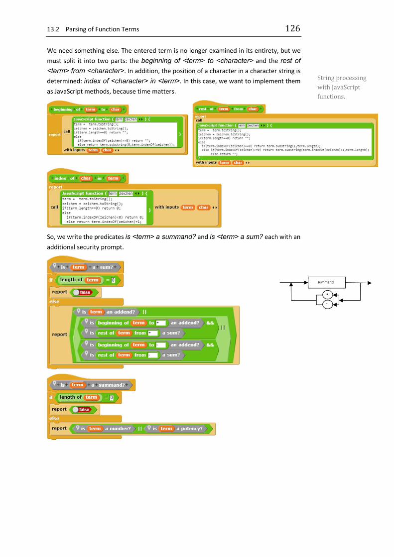
13.2 Parsing of Function Terms 126

We need something else. The entered term is no longer examined in its entirety, but we must split it into two parts: the beginning of <term> to <character> and the rest of

<term> from <character>. In addition, the position of a character in a character string is determined: index of <character> in <term>. In this case, we want to implement them as JavaScript methods, because time matters.

So, we write the predicates is <term> a summand? and is <term> a sum? each with an additional security prompt.

summand

+

-

String processing with JavaScript functions.


We are coming to the end. is <term> a number? is very easy to write when we have is <term> a cipher?

And how do you check a potency? That's also in the syntax diagram - we just have to copy all the details.

x

^ number number

13.2 Parsing of Function Terms 128

Now only the product is missing, which can be formulated in direct analogy to the sum, because a product consists (with us) of either a compounded sum or a sum followed by a product.

We can use it to check (parse) whether an entered term corresponds to the selected syn-tax. If this is the case, you can continue working with it. Our mathematician Paul here asks the Parser.

Of course, he packs this query in a separate block to give the impression that he can answer

something like this himself. 😉

also pretty recursively

sum ( )


13.3 Derivation of Function Terms

We now want to determine the first derivation of correct function terms. We collect the necessary methods from the parser again. Since there are only two possibilities for the internal structure of terms, the first approach is simple.

When applying the summation rule, we must determine and derive the summands. Because we have defined unsigned numbers, we treat them separately, that is, we add a "+" if nec-essary and then split the sign again. Then the different possi-bilities are treated according to the rules of mathematics.

When applying the sum rule, script variables were used for a change. This shortens the procedure a little bit.

13.3 Derivation of Function Terms 130

Only the product rule is still missing. We can just write them down - with the addition of some brackets.

The result can even be read to some extent:

It should be noted that the derivatives do not necessarily correspond to our simplified definition of function terms and therefore often cannot be "further processed".


13.4 Calculation of Function Results and Graphs

If we can parse function terms, then of course we can also calculate them. The procedure is very similar to parsing, and it is much easier if we already know that the term entered is correct. We leave this work to Paul, who up to now - apart from self-portrayal - was quite superfluous. But, as a mathematician, he can do arithmetic!

We want to calculate function values and then draw the graphs of the function and its first derivative. Paul must be able to draw at least one graph.

In these scripts all blocks already exist - except for one. The calculation of a function term at position x is still missing. We specify the corresponding scripts only because they are very similar to those of the parser.

13.4 Calculation of Function Results and Graphs 132


With their help Paul can now shine!

13.5 Tasks 134

13.5 Tasks

1. a: Make the outputs a little more readable. b: Combine results in the derivation so that they correspond to the given syntax and

the graph can be drawn. 2. a: Define signed numbers and change the processing of the terms accordingly. b: Proceed accordingly for floating point numbers (numbers with decimal points). 3. a: Define advanced function terms, which can contain quotients, using syntax dia-

grams. b: Enable parsing of these function terms by writing appropriate predicates. c: Form derivatives by implementing the quotient rule as a string operation. 4. Perform task 3 accordingly for trigonometric functions. 5. Allow function terms that require the use of the chain rule. Implement appropriate

predicates and string functions. 6. a: Let the graphs of the other function types draw after they have been parsed. b: Allow a selection of the graphs to be drawn (function, first and second derivation). 7. Introduce a "function calculator": a function term is entered first. If this is correct,

values can be entered repeatedly, and the corresponding values are determined.

14 Artificial Plants: L-Systems 135

14 Artificial Plants: L-Systems

Contents: using a list as a stack simple context-free language use of Turtlegrafik

14.1 L-Systems

In Aristid Lindenmayer's systems33, plants are described by a rule system that creates the drawing instruction for a turtle from an axiom, a first character, by substitution. One can imagine that - starting from a shoot - the plant is drawn until the next branching point. This position is stored on a stack, then the branches are written one after the other, returning to branching after each branch. Turtle masters only forward movement (F) and turns around a fixed angle (+ and -). Saving the turtle position and direction and restoring this state is symbolized by square brackets ([ and ]). A simple plant with a triple branch can be described by

axiom: X rule: X F[-X][+X]FX

If this rule is applied several times, the plant can grow at the positions where an X has been inserted. For the older parts of the plant to grow with it, a rule F FF is often added to the rule system.

33 https://de.wikipedia.org/wiki/Lindenmayer-System

shoot with triple branching

14.2 Create the Drawing Instruction 136

14.2 Create the Drawing Instruction

First of all, we need a rule system, i.e. a list variable rules, to which the desired rules are added line by line as character strings. The character to be replaced is at the very front, then follow -> and the replacement from character 4 onwards. The recursion depth, the specified angle and the length of the drawing path are also assigned to variables.

When creating the drawing instruction, we start with the axiom. Then we create an aux-iliary string h in which the substitutions are performed per run: whenever a character to be replaced is found in the old character statement, we append the replacement to h. Finally, h replaces the drawing instruction and the next replacement cycle is started.

14.3 The Stack Operations

We use a simple list as a stack for storing the turtle posi-tions. Operations are only performed at the top of the list - we already have a stack. Storing is usually done by a push operation. We store a three-element list with x- and y-po-sitions as well as the current direction. Use pull to retrieve the last saved position and remove it from the stack.

Preferences

The drawing state-ment can be quite long. Therefore "warp" is used to ac-celerate the whole thing.

14 Artificial Plants: L-Systems 137

14.4 Drawing the Plants

Drawing the plants is very easy because all our sprites can be used as turtle. We enlarge our working area to 500x500 (select stage size... in the Settings menu) and let the turtle draw the "foot" on which the plant grows. The character string is then processed character by character using the character instructions, with the corresponding turtle opera-tion or a stack operation being executed for each character. As a small delicacy we draw the "tips" of the plant green. (Peaks can be recognized by the fact that the next step is to return to the last turtle position, i.e. a pull operation follows.)

Examples:

14.5 Tasks 138

14.5 Tasks

1. a: Search the web for grammars for L-systems. Create the appropriate plants. b: Select a plant species, e.g. a certain tree species, and study its construction thor-

oughly using pictures. Pay particular attention to growth areas. Then describe their structure using an L-system grammar. Check the result using the program.

2. a: Why are the grammars considered so far "context-free"? What does this mean for

the plants produced?? b: Check the web to see if grammars other than context-free are used to describe ar-

tificial plants. If yes: why actually? 3. a: In the program the tips of the branches (as "leaves") were dyed green. Replace these

green pieces with more beautiful leaves. b: Transfer the principle to drawing the thickness of the branches. Just come up with

something! 😉 4. Plants don't always grow the same: there are storms, raging children, hobby gar-

deners, weather disasters, ... Bring some randomness into play to produce differ-ently shaped plants of the same type.

5. a: The stack operations were always performed at the top of the list. Could one also

take the end? If yes: why? b: Would something change if you insert at the beginning of the stack and remove the

positions at the end? If yes: why? 6. The users of the L-system program can enter anything else as grammar. Check their

entries with a parser before trying to create the plant. 7. a: How would the rules for L-systems be changed if we wanted to create three-dimen-

sional plants? What did this mean for the drawing of the plants? Are there turtles for three-dimensional drawing?

b: Find out about topics where artificial plants are used on the net. 8. Do they also draw artificial animals? Artificial people? If yes: where? How do they

do that?

15 Automata 139

15 Automata

Contents: finite automaton as a predicate hyphenation and pronunciation coupled Turing machines and control structures

15.1 Correct Mail Addresses

We want to use a finite automaton (FA) to check if a mail address is correct. To do this, of course, we must first know what "correct" means. We specify a syntax diagram:

mail address:

In this simplified form, the participant names consist of the characters a and 1 (as substi-tutes for letters and special characters) in an arbitrarily sequence, followed by the usual @. The mail server name consists only of b, and - separated by the dot - follows as domain name de.

For example, correct email addresses are [email protected] [email protected], [email protected] would be wrong.

a

1 @ b . d e

15.1 Correct Mail Addresses 140

Translated into a finite automaton we get its state diagram:

Translation into a Snap! script can well be done as a predicate, because the machine's response is true (the final state se has been reached) or false (another state has been reached, typically the error state sf). In the script, the checked address is scanned char-acter by character. Starting from the initial state s0, the system checks whether the current character is permitted. If it is, the sys-tem changes to the next state specified in the state diagram, oth-erwise to the error state. The script is quite long but consists only of nested alternatives that represent a direct translation of the state diagram.

When checking the mail addresses, the predicate created can be used.

a 1 @ b . d e

a 1 @ b . d e a 1 @ b . e

a 1 @ b . e a 1 @ d e

a 1 @ . d e b . d e @ b . d e

a 1

a 1 s0 s1 @

s2 b

s3

b

. s4

d s5

e se

sf

15 Automata 141

15.2 Hyphenation: Kevin Speaks34

Mealy machines can be used to implement simple hyphenation that works surprisingly well. In addition, we want to get Sprite Kevin to pronounce the entered words. The second sounds more difficult than it is: if we have the syllables, then for each syllable we can create an image with the mouth position whose name corresponds to the syllable (e.g. AU.png) and record the spoken syllable (e.g. as AU.wav). We drag these files into the Costumes or Sounds areas of Snap! and call them from there.

We start from the adjoining, very simple Mealy ma-chine. Its input alphabet consists of vowels (v), con-sonants (k) and other separators (t). It inserts some separators for hyphenation, but of course it works incompletely and partly wrong. It separates the strings vkv in v-kv and vkkv in vk-kv. First of all, we have to be able to enter a word into the program. For this we use the command ask and wait. The result is available as answer in the Sensing palette. This word is to be separated.

Since users of programs never follow the guidelines, we first make sure that only capital letters appear in the word. To do this, we must be able to convert at least one single character into uppercase if neces-sary. We have already written the function for this in Vigenère encryption, as well as the function for the conversion of whole words.

A word converted to upper case can be similarly trans-formed into a sequence of the characters v, k and t. The vowels are easy to find, the consonants are letters that are not vowels, the rest is treated as separators. For practical reasons, a t-character is added last. This means that at least one character is always present - and we always reach the state 0 at the machine at last.

34 based on an idea by Wilfrid Herget.

15.2 Hyphenation: Kevin Speaks 142

It's time to split the sequence. We read character for character v, k or t and write down our automaton: Depending on the state, the next state is specified, and characters are added to the output.

Attention: the states are handled by nested alternatives, so that after a change of state the following statement is not executed without a new character being read in first!

Finally, we must convert the vkt sequence back to the original characters - with the separators between them. To do this, we run through the vkt sequence with the separators (index: i) as a pattern and build the result sequence from the characters of the entered word (index j). However, we only change j if i does not point to a separator (-) in the pattern

We can now use these functions one after the other to separate a word:

And of course, we can bundle such instruction sequences in a new block.

15 Automata 143

The words, divided into syllables, should be pronounced by the computer, similar to navi-gation systems, automatic time announcements or other "computer voices". If we store syllables instead of whole words, we need considerably less storage space, because the syllables can be used several times. (But it doesn't get any nicer!)

First, we choose a few (here: German) words: Autobahn, autonom, Au-tomat, Pronom, Promille, Kamille, Kamel, Kaktus. For short syllables we can use the built-in sound re-corder. Or we speak the syllables (e.g. in Scratch) into the microphone and save the WAV files under the name of the syllable in capital letters. We drag the sound files into the Sounds section of Snap!

Since the entered words have been separated (see above), we get (approxi-mately) the syllables when we "decompose" the word. To do this, Snap! provides the split by command. The block creates a list of the parts of a word. If we enter Au-to-bahn and separate at the sign "-", then we get:

If our sound files have the same name as the syllables, we can play them with play sound

until done by selecting the syllable as input parameter of the block.

We can let the computer pronounce words by

separating the entered word and breaking it down into its syllables, from this list, "pronounce" the first element in

each case and delete it from the list until the list is empty.

15.2 Hyphenation: Kevin Speaks 144

For each of the different syllables we draw a costume for Kevin.

AU TO BAHN

These costumes are displayed while speaking the syllables.

Words are pronounced by calling this script with the corresponding syllables.

15 Automata 145

15.3 Coupled Turing Machines 35

If one describes Turing machines by state graphs, then the meaning, which is assigned to this model, seems to the learners strongly exaggerated, because the problems, which can be described by a still readable graph, are nevertheless quite simple. Much more powerful tools can be generated in the model of coupled Turing machines, in which the initial state of the next machine corresponds to the final state of its predecessor. More and more pow-erful designs can be created from very simple systems. The result is a kind of macro lan-guage in which topics of predictability and decidability can be formulated.

Our system of elementary Turing machines works on a Turing tape, which contains only ones and zeros. The zeros serve as separators, so that numbers must be represented by ones. The number n is coded accordingly by n+1 ones, so that the zero also has a code. In the standard position, the head of the Turing machine is above the one on the far right. All groups of ones must be separated by exactly one zero and there are two zeros at the left edge of the band. After the work the machine is back in the standard position. The next machine starts working out of this.

The 1- and 0-machines are available as elementary machines, which write the corre-sponding character at the head position on the tape. That's all they're doing. The small left

machine l moves the head of the Turing machine one position to the left, the small right

machine r to the right. There is also a testing machine p that checks which character is present at the current head position. Depending on the result, it branches into one of two states to which further machines can then be coupled. That's about it.

Because they are often needed, we design two new machines, the large left machine L, which runs to the left over a group of ones, and correspondingly a large right machine R. These can be realized as follows:

L: R:

The copying machine K1 copies a group of ones to the right.

K1:

If the copying machine K2 copies one group of ones over a second group to the right, then we can already calculate sums with the help of a Turingadder A by:

A: K2 K2 L 1 R l 0 l 0 l

Give it a try!

35 from Eckart Modrow, Theoretische Informatik mit Delphi, emu-online, 2005

l p 0

1

r p 0

1

p 0 R R 1 L L 1 l 1

0 R R l


Instead of testing the machines on paper, we want to develop a macro language in which our coupled Turing machines can be realized. Since we don't want to use the normal Snap! command palettes, we disable them after right-clicking on a palette (hide primitives). The palette is empty after that.

For the simulation of the machines, we need a tape consisting of ones and zeros. We choose a list tape, because it can be easily changed in length. For the display we create some images with ones and zeros of different sizes, whereby the head position is displayed in yellow. The working speed and the cell size should be changeable on the screen. Overall, we need the variables initial caption, tape, tape length, pos, cell type and pause(ms).

The initial caption must be asked, and an appropriate band must be generated and dis-played.

The default position must be taken on this tape, where the value of the variable pos is determined.

The tape is then displayed by "stamping" images of the costumes side by side on the stage.

15 Automata 147

Altogether we get as start command sequence:

To show the head position we calculate its screen coordinates and switch to one of the yellow costumes.

The elementary machines can now be quickly generated:

The generation of the testing machine p is somewhat more complicated, because it must be able to execute two different scripts - depending on the tape letter. These scripts must therefore not be evaluated as parameter values BEFORE the p-machine call is executed, but two scripts are passed, which are to be executed AFTER the call, depending on the tape labeling. The "parameter values" are scripts. When typing the parameters, we select Com-

mand (C-shape) to prevent the evaluation. The parameters are identified by a as scripts.

Use programs as data: C-shape code


With these machines, the others can be developed "normally recursively" in Snap! as blocks.

The work of the machines can be monitored and thus checked on the screen. So after that they are used as new blocks for more complex problems.

Instruction set of the Turing machines

15 Automata 149

15.4 Cellular Automata: Iterated Prisoner's Dilemma36

We want to build a cellular automaton based on the prisoner's dilemma37, but slightly modified for trading on the Internet. The behavior of the trading partners is simulated by machines that sit on a grid closed in both dimensions. They trade with the partners within a Von Neumann neighborhood. As is usual on the Internet, they exchange goods for money. There are different types of business partners:

Naive always cooperate, i.e. provide the correct equivalent value. Fraudsters never cooperate. Shrewd people cooperate at first and then react in the same way as their partner

did last time.

We describe the behaviour of trading partners using state diagrams:

K: „cooperate“

B: „cheat“

If we arrange such automatons in a grid, distribute them randomly and color them according to their state (green as "naive", red as "fraudster" or yellow as "shrewd"), we get an image similar to the following:

36 from Eckart Modrow, Zelluläre Automaten, LOG IN 127 (2004) 37 https://de.wikipedia.org/wiki/Gefangenendilemma

K,K v B,K

K

The „naive“

K,B v B,B

B

The „fraudster“

B,K

K,K

K

The „shrewd“ K,B

B,B

B

15.4 Cellular Automata: Iterated Prisoner's Dilemma 150

The further procedure is simple: First all partners trade once with their neighbors from the Von Neumann neighborhood, i.e. with the neighbors above, below, left and right. After-wards all partners evaluate the success of their neighbors. As opportunists, they take over the status of the most successful neighbor or maintain their status when they were better themselves.

In the first generations, the "fraudsters" usually prevail. But then clusters of "naive" or "shrewd" people form and a wild "battle" begins.

It is true that the "naive" are hard pressed by the "fraudsters". But they do quite well in groups. The "shrewd" usually prevail over the "fraudsters" - depending on the configura-tion - and cooperate with the "naive". In the end, the "shrewd" usually win - but not always. In groups, the "fraudsters" cheat each other and win nothing, while the "shrewd ones" assert themselves against them and are more successful with the naïve "behind their backs". The processes depend strongly on how the different behavior is weighted.

Global variables are suitable for evaluating the system, e.g. a "gross national product" as the sum of all trading points. Observing the sometimes surprising processes provides start-ing points for discussing ethical questions. Even if the example cannot, of course, be di-rectly applied to social systems, for most people we have found a new argument for coop-erative social behavior, which is not derived from transcendental or philosophical consid-erations, but from efficiency. It is in clear contrast to the egocentricity of primitive Darwin-ism, which often dominates public discussion in this respect. A diagram may serve as an example in which, on the one hand, the total numbers of the three types of automata (naive, fraudulent, shrewd) were plotted, and, in addition, the sum of the total trading points achieved by all types, i.e. the "gross national product", is somewhat thicker in blue. One can see very nicely that "social prosperity" (if one wants to derive this from the "trad-ing volume") is contrary to the number of "egoists" - of course under the conditions set.

15 Automata 151

Among them, fraudsters usually die out for lack of success, and the naive harmonize mag-nificently with the shrewd - if they are among themselves. If the behavior is weighted dif-ferently, fraudsters can be quite successful. So, it depends on the rules of the game who succeeds. You should think about them, not just in a simulation!

From a programming point of view, the system is rather simple, but sometimes extensive due to the change of viewing direction.

A new automaton can be described by a list of lists, whereby the automatons at the grid places correspond to sequences of numbers, which contain on the one hand their state and the reached trading points, on the other hand the "memory" about the past behavior of the neighbors.


The cellular automaton can be displayed by stamping different coloured costumes (small rectangles) next to each other on the work area. This has been changed to the size 800x600 pixels before.

Once the machine has been created, the new gen-erations are created from the last generation in each case.

The scripts have a very similar structure: a ll grid locations are iterated.

15 Automata 153

The trade of a cell with its neighbors depends on the one hand on the states of the partial machines, and on the other hand on their previous behavior. Since this data is stored in the machine values, it is easy to retrieve. Shown is the trade with the left neighbor:

determine cell

Torus world: the opposite edges are con-nected.

determine neighboring cell

is the cell cooperating?

is the neighbor cooperating?

save neighbor's behavior "for later”

if they both cooperate: profit between 2 and 10,

nothing else

the neighbor is cheated: profit between 1 and 20

cheat on both of them:

almost no profit

Trade with the other three neighbors is almost the same. The differences are only in the positions of the stored behavior.


Once the values of a generation have been determined, they can be counted and compiled in a list - and this results in a diagram.

15 Automata 155

15.5 Tasks

1. Develop a finite automaton as a predicate for detection a: correct license plates from three different cities. b: correct IBAN numbers. You can limit your search to a few banks. c: passwords of sufficient complexity. Define beforehand what "sufficiently complex"

means. 2. Improve hyphenation by taking into account a: double consonants. b: typical prefixes. 3. Develop and test a coupled Turing machine, a: that copies one group of ones over another (K2). b: which pushes one group of ones to the left to another until the groups are sepa-

rated only by a zero. c: which multiplies two natural numbers with each other. d: which writes a 1 after two groups of ones, if they are the same length, otherwise a

zero. e: that subtracts two natural numbers - if that's possible. If she doesn't, she'll go

crazy: she'll run away to the right. 4. a: Replace the trade of all partial automata with the neighbors "per round" by a ran-

domly controlled process in which machines trade with neighboring (with any) partners.

b: Replace the Von Neumann neighborhood with a Moore neighborhood. c: The machine can easily be converted to an Ising model by considering the ma-

chines as spin grids. Per round, the majority of the neighboring spins tilt the spin in the middle in their direction. There are various magnetized areas.

5. a: Find out about Stephen Wolfram's linear cellular automata. b: Implement the model.

16.1 LOGO for the Poor 156

16 Projects

16.1 LOGO for the Poor

Contents: 1. simple text-based programming 2. parsing 3. interpretation of input

We want to develop a small programming language that we can use to write programs for a turtle - that is, for every Snap! sprite. The project should show how a text-based lan-guage works and how the error messages are generated. We reduce the problem a little by allowing one-letter commands only. If we look at the possibilities of the pen used in Snap! and select some of them, we get a possible command set (very small here):

Mn moves the turtle by the distance of length n in the current direction Tn rotates the turtle on the spot by n degrees U lifts the pin D lowers the pin

We add a control structure to these four commands, here: a loop - and the minimal version of a programming language is ready.

Rn{ drawing commands }

We cast this rough sketch in the form of syntax diagrams: A turtle program consists of a sequence of commands separated by semicolons. The program ends with a double cross sign.

turtle program:

control instruction:

drawing instruction:

number: natural numbers

Programs are e.g.: D;R4{M100;T90};U#

M100;T90;M100;T90;M100;T90;M100;T90# D;R180{M200;T183};R360{M1;T1}#

control instruction #

drawing command

;

;

number R drawing command { }

U

number M

number T

D

The syntax diagrams can easily be extended by additional com-mands.

16 Projects 157

We assume that superfluous characters such as spaces are removed from the program first. We can achieve this, for example, by converting entered lowercase letters into uppercase letters and allowing digits and the four special characters ";", "#", "{" and "}". All other characters lead to the error message "ERROR 1: Wrong character in the input!".

A simple input method with character control.


The input must be checked to see whether it represents a permitted LOGO program - it is "parsed". In this case we can develop the parser as a finite automaton38. The unspecified transitions lead to an error state.

In the individual states we can decide which signs lead to subsequent states and which do not. This al-lows us to indicate which characters were actually expected in the event of incorrect entries. If we num-ber these error messages of the parser in the order of their occurrence, we get the adjacent table.

If we also evaluate the position of the character in the command where the error occurred, then we can even display the error.

The translation of the parser consists only of a very long copy of the state graph - of nested alternatives.

38 Why is that, by the way?

state possible error message S0, S6 2: unknown command S1, S10 3: <;> or <#> expected S2, S4, S8 4: number expected S3 5: number, <;> or <#> expected S5 6: number or <{> expected S7 7: <;> or <}> expected S9 8: Zahl, <;> or <}> expected 9: unexpected end of input

Se

#

;

U v D

S1

;

#

;

}

M v T

}

;

U v D {

S4

R

0 v 1 v … v 9

0 v 1 v … v 9

S5 S6

S7

0 v 1 v … v 9

S8 S9

S10

0 v 1 v … v 9

; #

0 v 1 v … v 9

0 v 1 v … v 9 M v T S0 S2 S3

16 Projects 159

The parser parse <program> is guided through the state dia-gram by the character string of the program. If there is no per-missible transition in a state, it reports the corresponding error by the value of the "result" vari-able. Correct programs have the value 0 as a result.

The rest of the state diagram.


The interpreter run <program> can assume that the entered program is error-free - after all it was parsed. Therefore, it can take the first character of the program one after the other - this is the next command - and delete this character. Depending on the command, it executes this and searches for the required parameters, e.g. the angle of rotation. All processed characters are deleted. This ends when the program consists only of the last character – the "#".

The program is processed charac-ter by character, the processed characters are deleted. We used the function all but first letter of <string> of the library words, sentences. PenUp command (U) PenDown command (D) search for a number Turn command (T) Move command (M) run the loop (R) Search for loop contents until the next "}"... ... and execute as often as the number indicates. Append a ";" to the loop contents.

16 Projects 161

If we output the error messages in plain text, then our programming language will slowly become usable.

We can evaluate programs through a short script.


Actually, it is a bit strange to develop a very primitive text-based language in a graphical programming language. However, experience shows that learners usually combine the work of computer scientists with the development of cryptic texts - i.e. they sometimes want to program "really". We can accommodate this wish if we use such a mini-language in a standard field of computer science, in this case automata theory. Since we develop it ourselves, we promote understanding for the processing of texts, which takes place on many levels in IT systems. In addition, we have found a highly differentiating topic suitable for division of work and challenging activities, which quickly leads to presentable results.

Tasks:

1. Expand the language LOGO by a: a Home (H) command that sends the turtle to the center of the screen. b: a Clear command (C) that clears the screen. c: a Color<n> (Fn) command that allows you to select a pen color. d: a command TurnTo<angle> (Nn), which rotates the Turtle to a certain angle. e: a command MoveTo<x><Y> (Vx,y), which sends the turtle to a certain point. 2. Develop a scanner that allows you to enter the turtle commands in long form, for

example, to write Turn 90 instead of T90. The scanner should recognize these commands and output them again in short form.

3. Introduce an alternative: Depending on the color of the pixel at the location of the

turtle, it should be possible to execute different command sequences. Reduce the syntax appropriately and implement the command.

4. Two types of loops are to be introduced in this way: The turtle should execute

drawing commands as long as (WHILE) or until (DO) the turtle is above pixels of a specified color. Allow position-dependent predicates as well.

16 Projects 163

16.2 SnapMinder by Jens Mönig39

Contents: import and visualization of large amounts of data advanced list operations connection to socially relevant issues The program is based on data from the Gapminder Foundation40, which pro-vides tools for visualizing statistical data on the Internet. One of these shows the development of the coun-tries in the recent past, whereby life expectancy is represented above in-come and the size of the "bubbles" corresponds to the total population of the country in one year. If you move the slider, you can impressively follow the temporal development of the countries in this coordinate system.

The data used - and many others - can be found in tabular form at https://www.gap-minder.org/data/

39 With permission of the author, available at snap.berkeley.edu/run#pre-sent:Username=jens&ProjectName=SnapMinder 40 https://www.gapminder.org/

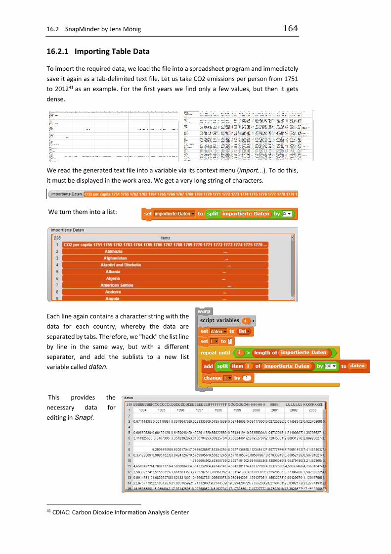
16.2 SnapMinder by Jens Mönig 164

16.2.1 Importing Table Data

To import the required data, we load the file into a spreadsheet program and immediately save it again as a tab-delimited text file. Let us take CO2 emissions per person from 1751 to 201241 as an example. For the first years we find only a few values, but then it gets dense.

We read the generated text file into a variable via its context menu (import...). To do this, it must be displayed in the work area. We get a very long string of characters.

We turn them into a list:

Each line again contains a character string with the data for each country, whereby the data are separated by tabs. Therefore, we "hack" the list line by line in the same way, but with a different separator, and add the sublists to a new list variable called daten. This provides the necessary data for editing in Snap!.

41 CDIAC: Carbon Dioxide Information Analysis Center

16 Projects 165

16.2.2 The SnapMinder Data

The program contains the required data as described above in the variables income data, life data und population data.

It prepares them for further use with the help of higher order list operations from the Tools library42. As an example, we show the population:

Convert the population data into a list (here in "one step") and throw out those "without interesting content".

Use only data from existing coun-tries.

Sort out unusable data ("... no numbers").

Format data separated by commas and with CR between the lines as population data - clean.

The operations are very compact due to their nesting. If you take them apart, they are easy to understand. Let's take the first nested block as an example. It can be read "from behind" as: - Split the population data, stored in a string separated by line feeds, into a list. Split this

list again. The contents must now be separated by commas (csv format). - Delete from the result all entries where nothing comes after the first entry. - Assign the result to the variable population.

42 Jens Mönig uses a little trick: If you move the block of a list operation over the join block from the string operations, which is displayed "empty" , i.e. without input parame-ters, then it turns into the join input list-Block , which converts the list into a simple string. The function can also be easily written by the user.


The program starts with three messages, which cause old country sprites to delete themselves, and the other objects, especially the data lists, to be initialized. For the data, it works like this:

Process the data as described above. First the income, ...

... then life expectancy, ...

... and extract the countries from it. Assign the income to the countries.

Same for life expectancy. Write back the population data from the auxiliary vari-able.

Set some variable values.

Extract the years.

Create a list of years as an index.

16 Projects 167

16.2.3 The SnapMinder Countries

At the start of the program as many country clones, represented by a semi-transparent rectangle, are created as countries are included in the country list. Each clone has its own index idx.

The main function of the countries is to position themselves in the coordinate system of average income and life expectancy in relation to the year under consideration. For this ...

… they determine these data for their country, ...

... determine the position ...

... and their size, which is given by the population of the country in the year un-der consideration.

This block is called, among other things, when a plot of the country, i.e. the movement in the coordinate system with the year as parameter, is generated.


16.2.4 Use SnapMinder

The presentation is impressive because, on the one hand, the countries move from bottom left to top right in the course of time, i.e. they develop positively. But if you take a closer look at some countries, this development is by no means continuous: there are abrupt downward swings, backward movements, circles, periodic movements,... The program gives rise to research into the causes of these developments, and there are a few surprises!

We show plots of some countries, then you should research! 😉

USA Germany

China India

Norway Somalia

16 Projects 169

16.3 Connectivity: The World is Small43

Contents:

1. topology of networks 2. extensive operations on simple lists 3. socially relevant issues

The handling of networks is often reduced to protocols and other technical details. But you can also ask other questions, e.g. about the connection of networks. If we have n nodes, how many links do we need for the network to be largely con-

nected? Or vice versa: How many and which nodes must be destroyed for a network to break

up into its subnets? Or: What is the mean distance, counted in links, between the nodes of a network?

Nodes and links can be very different in nature. It can be e.g. technical links between computer systems, customer/supplier relations in the economy, the logical connections via linked websites, social relations between persons or groups of persons hydrogen bonds in organic compounds, neuronal networks or infection chains.

43 from: E. Modrow: Informatik mit Delphi – Band 2, emu-online, 2003

16.3 Connectivity: The World is Small 170

16.3.1 Random Networks

The starting point for such questions were Random Networks. They are created when we build N network nodes (or pages, ...) that we subsequently link to each other. Let us take the Internet as an example. If there are N pages with on average k links per page, then with n mouse-clicks kn pages are accessible. We can reach virtually any page if it is: kn = N

n = log N / log k. With 5 billion pages and k = 7, n = 11.5, i.e.: with about 12 mouse clicks on average, you can visit any page of this network. Similar considerations and prac-tical studies have been carried out on social relations, etc. They can be found under the name Small World Phenomenon44.

If you display the distribution of links per page, you get a Poisson distribution for Random Networks.

It is somewhat more difficult to decide whether a net-work is (largely) coherent, i.e. whether all nodes are connected to each other. We can answer this question by coloring: start with one node and color all the nodes that can be reached by it in the same color, then a co-herent network shows a kind of phase transition: al-most suddenly all nodes take on the same color.

You can see that the network - with the exception of a few slips - is coherent if the number of links roughly corresponds to the number of nodes. Further links do little to change.

44 https://de.wikipedia.org/wiki/Kleine-Welt-Ph%C3%A4nomen

16 Projects 171

16.3.2 Scalefree Networks

Albert-László Barabási45 showed in 2002 that growing networks like the Internet have a different distribu-tion of links per node than Random Networks. It can be described by a Pareto distribution. Brief descrip-tions can be found under

http://barabasi.com/f/623.pdf or http://barabasi.com/f/624.pdf.

A Scalefree network can be created by alternately adding nodes and links where the new nodes have two links to existing nodes. The older nodes are more likely to be linked than the younger nodes. Because the network is always coherent, there is no need to color contiguous nodes. But we want to make the size of the nodes dependent on the number of their links.

Scalefree networks are the same on all scales, i.e. numerous nodes with few connections are connected to a few nodes with many connections, so-called hubs. The connections between nodes normally run from the start node to the next hub, then via a few more hubs to the target node. Hubs can be, for example, people with many contacts (teachers, representatives, ...), central computers or distribution centers in merchandise manage-ment.

Scalefree Networks are extremely robust against technical faults. For example, if a network connection happens to fail, it probably does not affect a hub, and if it does, other hubs will compensate this. However, they are also extremely susceptible to targeted interference. If only a few hubs in this network type are destroyed, the network disintegrates into its individual parts.

45 A.Barabási: Linked: the new science of networks, Perseus Publishing 2002


The topic is suitable as an introduction to discussions about vaccination protection, pre-venting the spread of diseases, influencing political opinion-forming, optimizing the flow of goods, ...

16.3.3 The Implementation

We want to create a fairly simple model as a tool for researching network properties. It is essentially based on a node from which clones are gener-ated and two lists, of which the node list contains the nodes already gener-ated and the link list consists of sub-lists with the numbers of the two end nodes of the links. With their help, methods can be implemented largely independently of each other. They are used by the operating elements shown. The controls depend on the selected net type (random/scalefree) and the display of the nodes (rectangular/round with different sizes).

Buttons for switching between net types or for creating 10 nodes react to mouse clicks:

Since we often have to iterate over such node lists, we introduce a new control structure that exe-cutes an instruction for all objects in a list:

This makes it very easy, for example, to display all nodes:

node list and link list

16 Projects 173

New nodes are created by cloning the prototype. The prototype can be asked to perform this action.

A new link is inserted into the network by trying to find two nodes that are not yet connected. The link list must then be searched to see if the link already exists. If not, the search returns 0.

This allows the ends of the link to be determined. Since the resulting nets are quickly becoming large, the search for them does not take too long.


Once you know which nodes are to be connected from a link, ...

... then the affected nodes are searched for, ...

... the costume according to the net type is selected, and the knots are asked to change to it.

The pen is asked to draw a line be-tween the nodes.

Finally, the new link is entered in the link list and the related nodes are col-ored in the same way.

With Scalefree Networks it is a bit eas-ier, because the costumes are chosen randomly.

16 Projects 175

The most complex part is the coloring of the connected subnets. We work with two lists, from which the connected nodes get all nodes that can be reached from the starting node. The nodes to be colored contain the nodes that have to be colored – sic.

We start with the given node number as the beginning and remember its costume.

As long as there are still nodes in the list, we examine the link list to see if the first node number of the connected nodes ap-pears in the link either to the left or right. If so, the other node is also connected to the source node and is added to the list if it is not already in the list.

If the first node in the list is not yet con-tained in the list nodes to be colored, it is entered there and removed from the list of connected nodes.

Finally, the costumes of all nodes to be colored are set to the same value as the costume number of the initial node.

The controls, the two (and further) net types, the creation, joining and coloring of nodes as well as the diagram creation are based on the sub-lists and can be developed largely independently of each other. The topic is therefore well suited for teaching in different working groups.

16.4 Evolution 176

16.4 Evolution

Contents:

simple event control with buttons easy access to objects simple use of lists

The aim of this small project is to produce a presentable result with the simplest possible methods, which can be used in class if required. The methods, e.g. for the representation of the animals, are partly found by "trial and error", which of course challenges improvements. That's the way it's supposed to be. The starting points of the parts are somewhat highlighted in the pictures.

In the project, "animals" are randomly created, each consisting of 9 rectangles of random size, which are rotated to create a kind of horse. With a different composition, other "ani-mals" can be quickly produced. The partial rectangles are always drawn in the same order and orientation, so that you have to try out where to start drawing. Of course, this problem can be solved more elegantly with some mathematics, and if parameters can be used to influence how a rectangle is drawn, then it can be done more beautifully - in a different way. But it can also be done quite simply.

After the production of two animals, four offspring are created and shown slightly smaller below. From these you can choose two and appoint them as new parents. If you repeat this, you can "breed out" certain characteristics, e.g. small heads or short legs. At each crossing, the characteristics are changed at random. If a part becomes too small, it falls away. So you can breed something like seals or ostriches out of the initial horses.

It makes sense to create new parts by mutations or to change the starting point of the parts, i.e. to let them "migrate". To do this, the data structures must be changed, for ex-ample by recording the coordinates of the approach points and adjusting the methods ac-cordingly.

16 Projects 177

New animals can be created from the object Ani-

mal, which has a local method for this. In it, the parts of the animal are generated as lists of "reasonably usable" random numbers. They are then combined to form the complete list.

The parts of the animals are always drawn with the same method show part. The pen moves to the hor-izontal position and rotates to the angle passed as the third element in the list, then draws a rectangle with the lengths passed as the first and second ele-ment. In addition, the starting point is emphasized somewhat.

The method show animal first changes the size of the animal as indicated. Then the parts are drawn at the "tried out" points. Only the first part of it is shown.

16.4 Evolution 178

Two animals are "crossed" by randomly assembling the parts of one or the other animal into a new one. During each of these processes the dimensions are changed randomly - depending on the mutation rate mr.

Select from which animal a part will be taken.

Change the width of the part at random.

Too small parts fall away.

also, for the height

Add part to new animal.

Return result.

A new experiment is started by asking the Animal object to create two new animals as father and mother. They'll be crossed.

This is done accordingly with the children.

16 Projects 179

Let us try to breed "jumping ponies" with short tails. First we create the parents and select candidates for ponies from the offspring.

Well - evolution is just unfathomable! 😉

16.5 Using the Sensor Board Calliope 180

16.5 Using the Sensor Board Calliope

Contents: access to external hardware physical computing access to current topics (“smart watch”) We use one of the standard sensor boards, in this case the Calliope

mini. For this, there is a program by Andreas Flemming46, which contin-uously sends the measured values of the board via an internal server and thus also makes them accessi-ble to browser applications via the http protocol. If we start the program, the Calli-ope board is found after a short search and the measured values are displayed.

The measured values are in the sequence acceleration in x-, -y and z-direction, state of buttons A and B as well as brightness and temperature, each in free units. We can easily split this string. Afterwards the individual values are accessible as contents of a list.

In a small script, based on an idea by Annika Eickhoff-Schachtebeck 47 , we try to convert the acceleration sen-sor in the x-direction into a step counter, as it is used in smart watches. We therefore attach the sensor board to the arm or leg and display the measured values graphically. (However, we should have a long enough cable between board and computer!)

46 https://www.uni-goettingen.de/de/software+zur+verwendung+des+calli-ope+mini+mit+scratch+1.4%2c+byob+und+snap%21+%28andreas+flemming%29+down-load/569672.html 47 in https://www.uni-goettingen.de/de/unterrichtsbeispiel+fitnessarmband+%28dr.+an-nika+eickhoff-schachtebeck%29+download/565581.html

The Calliope board as a pedometer.

16 Projects 181

The result is graphically available here, but can of course also be stored and evaluated as a series of measured values.

As an example, we enter the x-acceleration and the corresponding time of the measure-ment to a list.

These data must be smoothed for an evaluation, e.g. using an averaging of adjacent values, and then the maxima of the measurement series can be determined for a step count. Both are nice detail tasks. If we assume an average step size of 1m, then we can also determine the speed - and display the results. These can then be easily compared with those of commercially available devices. They're often

no better. 😉

16.6 Rate Websites: PageRank 182

16.6 Rate Websites: PageRank48

Contents: search engines OOP techniques current political issues If you know the addresses of websites, you can reach them directly via the net. But what happens when we search for pages with specific content? For this purpose, of course we use the search engines, which propose us to certain keywords network addresses from their tables of contents. These directories can be created by web crawlers automatically visiting as many accessible websites as possible, jumping from link to link, and adding the keywords found there to the table of contents of the search engine. This usually results in extremely extensive address collections for the same keyword.

Since users of search engines cannot handle large unordered address collections, the pages found for a keyword must be sorted according to their importance. Users then usually use relatively few addresses that appear first. The links below are hardly noticed. So at least the commercially operating providers on the net must be interested in appearing as high up as possible in the lists created by search engines in order to be found by potential cus-tomers at all. They use all tricks to achieve this.

So far, nothing has been said about the meaning of a page's information for the keyword. Just showing up doesn't mean much. For example, if a page contains the text "Nothing is written here about Göttingen", it will still be included in the table of contents relating to the keyword "Göttingen". So, we need other evaluation criteria. In the simplest case, the authors of a web page enter keywords in the meta tags for the content of the page:

<meta name = "keywords" content = "Snap!, school, computer science">

However, this possibility is often abused by using frequently used keywords - which do not affect the page content at all - to direct potential "victims" to the site. Not very helpful is the idea to count how often the keyword appears on the page. In this case, web pages sometimes contain certain keywords "invisible", e.g. by writing the keyword very often in white on a white background. Of course, you can also have people rate websites and enter them in the search directories. But this is a very expensive and relatively slow way to create directories, and of course such an evaluation is subjective. It is also often difficult to eval-uate pages with special content - e.g. from archaeology. In the worst case, the "value" of a page does not result from its content, but from the amount paid for the evaluation.

Another way to use the expertise of web authors for the evaluation of web pages on the one hand and to automate the evaluation process on the other hand is realized in the so-called PageRank procedure. Unlike the meta tags that evaluate your own website, links from one website to other websites are seen as a knowledge-based vote by which authors indicate that other websites contain interesting content. If someone refers to a page with physical content, the author will most likely understand something about the content.

48 from: E. Modrow: Technische Informatik mit Delphi, emu-online, 2004

16 Projects 183

Moreover, since it is usually not known which other websites refer to their own, web au-thors can only manipulate this procedure with difficulty.

The PageRank method does not evaluate all links equally. It determines a rank (the Page-Rank) for each known website, which describes the "weight" of this page. This rank is di-vided during the "vote" by links to all references leading away from the page. If a web page contains only one outbound link, then this receives the entire weight of the page, if it con-tains two, the weight is halved, and so on. (If the page does not contain an outgoing link, it will not take part in the vote. In the PageRank calculation, it returns the value 0.) The rank of a website increases if as many high ranked pages as possible refer to it and if these pages contain as few links as possible.

As a first example, let's choose two pages that mutually refer to each other. To calculate the PageRank of page A - PR(A) - we need the PageRank PR(B) of page B, because a link from B leads to page A. The calculation of PR(B), however, again includes PR(A). So, we need an old value of PR(A) to determine the new one. Since this argumentation can be continued, a method must be developed to reduce the influence of the old values on the calculation of the new rank, so that a stable result is obtained in the course of the calculations. This is achieved by multi-plying the contribution of the incoming links by a factor d which is less than 1. Since this is included in every calculation, the "very old" PageRanks are multiplied by dn, a number that is increasingly approaching zero. For example, you select the value 0.85 for d. If we desig-nate the times at which the PageRank was calculated in the past as t1, t2, t3, …, whereby a larger index should mean an earlier time, then for both our web pages we get:

...)(85,0...85,0...))(85,0(...85,0...)(85,0...)(3321

2 APRAPRBPRAPR tttt

If page B had more than one outbound link, we would have to divide its rank in the calcu-lation by the number of links - C(B). We must proceed accordingly with the other sites that have links to page A. If we call these n web pages T1, T2, …, Tn and replace the three dots in the above relationship with (1-d), then we get the original formula that was initially given by Google for the page rank calculation:

The rank of a website is at least 0.15. But what influence do the other terms have? We want to clarify the question with a simulation program in which symbolic web pages can be created and linked. The PageRanks can be calculated in a "website" created in this way.

page A

page B

85,0),)(

)(...

)(

)(

)(

)(()1()(

2

2

1

1 dTC

TPR

TC

TPR

TC

TPRddAPR

n

n


In our program, in addition to the buttons shown, which serve to control the functionality, we need the prototype of a "Page", which (here) should be a website, as well as a global list of all generated pages. Each page contains a link list with the numbers of the linked pages, a number, a PageRank PR and a help variable PRnew, in which the newly calcu-lated PageRank is added up.

Pages can be displayed on the screen. Since text and numerical values as well as some lines are to be drawn here, we use the already developed graphics library.


The most important task of the prototype is to create clones of itself. We save such a clone in a script variable result and ask it to perform the operations that produce the desired result through a sequence of commands. The generated page is added to the page list.

In the corresponding mode, pages are con-nected by clicking on two pages in succes-sion. The numbers of the affected pages are stored in two global variables. Then the first one can be asked to "link" to the second one. The Pen draws a line be-tween the sides that decreases in thick-ness, a kind of arrow. (Mutually connected sides thus maintain a connection almost the same thickness.) The second page is in-serted into the link list of the first page.

When recalculating the PageRanks, each page must distribute its current value to all connected pages. The page calculates this value and asks all pages of the link list to increase their auxiliary value PRnew accordingly.

16.6 Rate Websites: PageRank 186 You can use these auxiliary methods to calculate the pageranks. First of all, all auxiliary variables of the involved pages are set to zero. Then all pages distribute their values to the connected other pages. When this is done, the auxiliary variables are copied into the PR variables and the pages are redrawn with the new values.

We now want to use our simulation program. We create two websites, link them and calculate the PageRanks. You can see that the values converge towards 1 (independent of the initial PageRank, by the way). This is of course no surprise, because this is exactly what we intended to achieve with the introduction of the "damping factor" of 0.85.

As next example we choose the structure of a typical homepage with a tree structure, which starts from an index page and branches to subdirectories.

16 Projects 187

We now assume that there are additional external sites that link to our homepage.

The PageRank of the homepage increases considerably, also the weight of the internal pages increases.

Finally, we want to assume that the external pages are again referenced in a link list of the homepage.

The rank of the homepage continues to rise. One can see how the importance of the pages is growing in a network of pages that mutually refer to one another in order to express their "respect" for one another.

The PageRank procedure is a technical process that can also be transferred to other, e.g. social systems. How-ever, it quickly leads to socio-political questions, be-cause the focus is not on the content of the pages, but on their structure and functionality.

1. If the result of the PageRank calculation is decisive for the "visibility" of the pages49, why are commercially oriented private companies allowed to decide on this visibility?

2. The intelligence of the system results from the expertise of those who have consciously set links in very different areas. Isn't the result actually a public good that should be available to everyone without some profit (and power) from it?

3. If only the PageRank would be decisive, the search results would always have to be arranged in the same order. Obviously, this is not the case: the results differ depending on the person who is looking for. They are filtered according to their interests assumed by the search engine. In extreme cases, you only get the results that you want to see - or that someone thinks you want to see - or that someone thinks you should see. The political consequences (keyword: "echo chambers") are currently under discussion.

49 What only appears at the back is practically non-existent on the net.

17.1 Warehouse Management with SQLite 188

17 At the Supermarket50

In the following, rather extensive project we will work in different groups in the same context: a supermarket. On the one hand, technical questions are clarified and “specialist” methods are applied, and on the other hand, these questions are intended to give rise, for example, to the social effects of the technology used. The aim is to show that a system that is only one-sidedly geared towards the "automation" of its tasks can get pretty out of control. The conflicts of interest that arise between the supermarket on the one hand, whose employees want to do their work efficiently and well, and the customers who want to see their privacy protected, obviously require legal regulations in order to achieve a balance of interests. When working on the subproblems it should be experienced that there are very different ways to solve the problems. Of course, the various solutions also have different consequences - and vice versa: if certain consequences are undesirable, then one can always try to find other solutions that avoid these consequences. Technical decisions are almost never "without alternatives". Presenting them in this way shows quite clearly that a discussion of their effects should be avoided.

We imagine a supermarket with different departments:

a scanner cash register (reads barcodes on the products, supplies article numbers and invoices)

a warehouse management system with integrated database (receives article num-bers, supplies prices and, if necessary, orders products from suppliers)

an "intelligent" scale for fruits (recognizes a fruit with the help of a camera, gen-erates barcodes)

an advertising department (responsible for payback, advertising, special offers, ...) a security department (responsible for the payment of parking fees, customers

with house ban, ...)

The implementations of the individual departments run on different computers and are processed by different groups. They communicate via a database on a server. And we do not use professional procedures, but only "naive" solutions that challenge improvements.

50 from E. Modrow, The SQLsnap supermarket, Scratch2015 Amsterdam

17 At the Supermarket 189

17.1 Warehouse Management with SQLite

The warehouse management must be accessible. In this case we use a small http server with "built-in" SQLite database by Andreas Flemming51, which we can start with one mouse click. Then a menu window opens in which we select the desired database - here the database supermarket.

There we find five tables:

products(pnr,identifier,maxstock,minstock,stock) suppliers(snr,supplier,zipcode,city,streetno) prices(pnr,snr,price) fruits(fnr,fruit,shape,size,colorcode) facerecognition(name,noseToEyes,mouthToEyes, mouseToNose)

We created this database e.g. with SQLiteAdmin52 and filled it with data.

For the SQL server, we first import the SQLite blocks library and the Sprite SQLite server (and thus also the required variables and access methods) in this order into an empty project. (We may also need the library "Web services access (https)" from the file menu, depending on the configuration of the server. For the sake of beauty, we take a picture of a warehouse as a costume of a sprite warehouse, send it to the correct position and make an stamp. Of course, we let the server establish the connection. We summarize the corresponding instructions in the block Init as a local method of the warehouse.

Our warehouse is waiting for the requests of the other departments of the supermarket. We leave the implementation of our own functionalities such as the automatic replenishment of stocks or the adjustment of prices to the tasks. However, in order to be able to answer inquiries, the warehouse establishes the connection to the database when the green flag is clicked.

51 http://www.uni-goettingen.de/de/http-server+mit+sqlite+f%c3%bcr+snap%21+%28down-load%29+andreas+flemming/582081.html 52 Using a free tool, such as SQLiteAdmin, you can easily create databases and tables and en-ter data.

17.1 Warehouse Management with SQLite 190

Our SQLite server can only do a few things: connect and compile the results of SQL queries.

For example, we receive all products with

In addition, we give them the option of listing the tables available in the database and displaying the attributes of a table.

For example, to display all products, we compile a corresponding SQL query:

If you want to change data in the database, use INSERT..INTO...- or UPDATE...SET...- statements..

Attention: Character strings must be enclosed with apostrophes!


Tasks:

1. If some products have been sold, the inventory has fallen below the minimum value minstock. Order new products so that the maxstock level is reached again. Find the supplier with the lowest price for this product.

2. The supermarket wants to become an "organic supermarket". Change suppliers for all

relevant products and adjust prices. 3. Add organic products and their prices to the product table in addition to the cheap

products - if possible. 4. Every Saturday evening an update process is started in the warehouse because the

prices of the suppliers may have changed. In this case the product prices have to be adjusted.

5. The supermarket works well but needs more money. Increase all prices by 10%. 6. The warehouse management needs statistics on sales per month and year. Collect the

necessary data and display the sales in suitable diagrams. 7. Write a block for delete statements for SQLite. Syntax: DELETE FROM <tablename> WHERE <condition>; Example: DELETE FROM suppliers WHERE supplier = ‘Miller’;

17.2 The Scanning Cash Register 192

17.2 The Scanning Cash Register

We have already dealt with a barcode reader before and therefore no longer have to deal with all the details here. For the sake of beauty, we take a picture from a scanner checkout as the costume of a sprite ScanningCashRegister, send it to the correct position and make a stamp. We summarize the corresponding instructions in the Init block as a local method of the cash register, which is called when the green flag is clicked. Additionally, we import the sprites Barcode and Laser from the old project barcode scanner.

We receive barcodes from the sprite Bar-

code. If this is visible, the laser can determine the EAN code. The re-quired variables and methods were im-ported as local varia-bles. With their help the scanner determines the product code (which here must be smaller than 17) and asks the server for the price.


Tasks:

1. Draw some new costumes for a printer sprite that can print barcodes on the stage. First, the user should be asked for the number to be displayed.

2. Search for information about your national barcode system. In Europe you will find EAN codes. Change the printer sprite to a "national printer sprite" that prints these codes.

3. If the warehouse management does not know the price, an appropriate response should be made. Change the script to a usable version.

4. If the warehouse management works correctly, the cash register should provide ans-wers in the form <price>,<name>. Make sure that.

5. Have the cash register produce invoices for the customers, including the date and time as well as all purchased products with prices and the total amount. Taxes should be declared as usual in your country.

6. The laser works quite slowly. Increase its speed.

7. Instead of always asking for individual data, the cash register can also get the current prices of the products in the morning and then work with this copied data. Change the system accordingly.

8. The warehouse can add new products to its database by reading the EAN codes at the

checkout and entering the remaining data manually. Implement this option.

17.3 The Smart Scale 194

17.3 The Smart Scale

A sensation is looming in the supermarket: the fruit department has ordered an "intelli-gent" scale with a camera that is supposed to recognize and weigh fruit at the same time. Unfortunately, only the camera is included, the fruit recognition has to be implemented by yourself. The fruit department gets help from the staff of the scanner cash register, be-cause they have already done similar things.

First, we try to find some criteria to distinguish fruits. We draw an apple, an orange, an apricot and a banana. The differences are obvious: apple and orange are round, the banana is long orange, apricot and banana are orange-yellow, the apple is (in this case) green the apricot is small, the others are bigger

But what do "round", "long", "yellow" and "green", "big" mean???

We know it, but the computer doesn't. We have to teach him.

We bring the object into the middle of the stage and send the laser from left to right and from bottom to top over the image. We measure the size of the object on these routes and calculate the ratio of the results. "Round" objects should have a ratio close to "1", "long" objects others. For "oval" objects we should actually use several measuring directions. But for us "oval" means "not round and not long".


The determine horizontal dimensions - block of the laser provides a list with two values: left and right border. Correspondingly, the determine vertical dimensions - block lower and upper limit of the object. With these results we can decide whether an object is round, long or oval. And we know its size.

The color of the object is still missing. We import the already known library and use the blocks to determine the dimensions of a costume and to determine an RGB value.

With their help we measure the color values at 5 points on the vertical and horizontal centerline respectively and determine the mean value from them.


Using these methods, the laser can determine the characteristic properties of a fruit.

Normal fruits have different colors. But our RGB values can display 256 * 256 * 256 colors, so 16,777,218. That's a little too many. We need a method to reduce the number of colors.

We try this: for each RGB channel we decide whether the color value is "high or "low". If it is high, we set it to 255, otherwise to 0, so we only get two possible values for each channel, so 2 * 2 * 2 = 8 possible colors. With this procedure we try out whether we can see anything useful at all - or not.

It's looking good, isn't it?

So, we can equip the fruit scale with a method that asks the laser to determine the fruit data.

17 At the Supermarket 197 And this result is used for a database query on the SQLite server. The color space is re-duced as discussed and the quotation marks are placed around the data.

It's working!

After these successes the crew of the fruit scale becomes courageous and tries to analize real fruit pictures.

It reduces the number of colors as described...


... and think that's enough. It'll take a while, but they've got time.

😉

Finally, they calculate the average colour of the fruit as indicated and reduce the result again. If they do that with an orange, they get a pretty yellow.

This means that the database can also be searched for "real" fruits - what more do we want?

17 At the Supermarket 199 Now you have the full toolbox together for optical fruit determination:

1. Take a picture of a fruit and choose it as the costume of a sprite. You can take pictures with your smartphone or laptop camera. The background should be white.

2. Reduce the color space of the image. 3. Measure size and shape of the fruit. 4. Measure the mean color of the fruit and reduce it as well. 5. Calculate the color code of the fruit.

The obtained data shape, size and color code can be used as columns of a database table. We will have three different values each for size and shape as well as 8 possible color codes. This allows us to distinguish 3 * 3 * 8 = 72 fruits. Try a "real" intelligent fruit scale in a

department store - we're not that bad. 😉

Tasks:

1. a: Create a database table for fruits of the following type: pnr fruit shape size color code 123 red apple round big 100 223 cherry round small 100 456 banana long big 110 … … … … …

b: Add the table to your database.

c: Write an evaluation method so that it provides the name and price of the fruit. To

do this, use database commands. 2. The color reduction process is very coarse. Come up with a better way. 3. Our fruit recognition process only works well if the fruit is placed in the center of

the stage and aligned horizontally. If we fit a sprite with a fruit picture as a cos-tume, we can center and align the Sprite in the middle before we print the cos-tume. Implement the procedure.

4. If we use a more detailed color code, we can distinguish more fruits. Would that

be progress in any situation? 5. It could be that the background of the fruit is not white. Can you help? 6. You can drastically reduce the duration of color space reduction by using Jens

Mönig's pixel library instead of getRGB... Do that. You can use the "light of old stars" as a template.

17.4 License Plate Recognition 200

17.4 License Plate Recognition

The success with the smart scale goes through the department store like a wildfire. It also reaches the security department. Among other things, it is responsible for the parking gar-age. To simplify the payment of parking fees, the department installs automatic license plate recognition. Registered customers with a customer card and automatic billing no longer have to stop in front of the parking garage barrier - at least that's the hope.

Car license plates contain special character sets that facilitate character recognition by computers. In Europe they have a black border - and that is good for us. So, let's try to determine the numbers on the plate. (We leave the other signs to you.) Fortunately, we have already realized almost all tools for our project. All you have to do is ask the people at the smart fruit scale!

We are trying to develop an extremely simple method of license plate recognition. The result is very sensitive to changes in position and size of the license plates. But these disadvantages can be easily corrected by using a detailed measurement method. Take a look at the exercises!

OCR (Optical Character Recognition) uses complex methods, often with neural networks, to recognize characters. Here we are inventing a simpler procedure that is similar to that of the smart scale. Because all our marks on the license plate are the same width, we can easily identify them once we have found the boundaries of the license plate. With the in-telligent scale you can see how this happens. We continue to use their laser.

We can produce license plates quickly with the help of various generators on the Internet. We save them as costumes of a sprite LicencePlate.

We start by searching the top and bottom of the license plate for lines that do not contain black pixels. Their positions indicate the upper and lower edge of the relevant characters. Then we search from left to right for vertical lines with black pixels. When we find the first one, we also have the beginning of the first character. Then we search for the first vertical line without black pixels. Their x-position is the end of the first character. We have a "win-dow" with the first sign in it. The next line with black pixels gives the width of the gap between the characters.


Now we can move this window over all characters of the license plate and try to recognize the characters inside the field.


We can move a red rectangle across all characters by first determining the character width and the gap between the characters.

The number recognition itself is still missing. As a starting point we take the characters with the rectangle around.

We imagine a "sensor field" consisting of three crossing lines. We measure the colors at the round points. We number the points as shown and look at the results in tabular form. (gray fields: result difficult to predict)

char P1 P2 P3 P4 P5 P6 P7 P8 Code(s)

0 00100100

1 01111110

2 01101010

3 01011100 01111100

4 11010001

5 00001100

6 0100100

7 01111010

8 00010100 01010100

9 00101100 00101110

Errors may occur with characters 3, 8 and 9 if the points are not very well adjusted. But that doesn't matter, because if we move the sensors P2, P3 and P7 a little bit so that they provide clear values, we can even do without the sensors P1, P2 and P8 (e.g.) and still have a usable code.

P8

P4

P1

P2 P3

P5 P7 P6


A possible layout for the remaining sensors would be:

We choose a license plate with all ten characters. The sensors are placed in suitable places (here: (14|24), ...) and stored in a list to read the colors in the character window at the positions and to form a code number from the colors interpreted as a dual code. When we're done, we transform the code into the right character.

char P1 P2 P3 P4 P5 P6 P7 P8 Code Wert 0 10010 18 1 11111 31 2 10101 21 3 11110 30 4 01000 8 5 00110 22 6 00010 10 7 11101 29 8 01010 10 9 10111 23


Now the security department can ask the laser from their office in the car park which car has just arrived:

The result is particularly impressive for the advertising department, which immediately sees completely new applications for the process. Everyone's very proud of the security!

Tasks

1. In the examples, the sensor positions are given absolutely in pixels. Address the sen-sors relative to the size of the character rectangle.

2. Character recognition in the examples is very simple, but very sensitive to changes in

the size and position of the license plate. Use more sensors to detect the characters more reliably.

3. Extend character recognition to the entire character set for vehicle license plates. 4. Character recognition programs can learn. If the script does not find any recognizable

patterns, it should display its result and ask for the correct character. Save the pat-terns and the corresponding characters in a database table. Use queries to identify unknown patterns.

5. If you want to read dirty license plates, you won't find any sharp character bounda-

ries. As a result, some sensors will produce errors. Improve the results in such cases by determining the "next correct code" of an incorrect code.


6. The recognition of dirty plates can be improved by converting the color image to a pure black-and-white image and closing the gaps caused by the dirt. Find out about suitable procedures for this purpose and implement one of them.

7. The security department needs a database of license plates and vehicle owners and

their status (customer, company member, unwanted person, external parker, etc.). Can you help?

8. The license plate recognition turns out to be a great success for the security depart-

ment. All its members are very proud of it and the other members of the company admire the "sheriffs". The advertising department now wants to use the data from the license plate table to honor customers as VIP customers who are frequently and for a long time present in the supermarket. These have special parking spaces near the elevator. Write a query to find VIP customers.

9. After some time, the VIP parking lots are occupied by pensioners and unemployed.

Therefore, the advertising department extends the criteria for VIP customers by a minimum of turnover with their purchases. Because almost all customers use credit cards for payment, this is no problem. Improve VIP customer query accordingly.

10. The advertising department finds that it would be helpful to know not only a custom-

er's turnover but also what they have bought. If it knows the interests of customers, it can provide them with special offers and special prices. Determine the additional tables required for this and their columns in the database. Write suitable queries.

11. The advertising department wants to know whether its advertising activities are suc-

cessful. Do they reach customers? Try to answer these questions based on the stored data.

12. On German motorways, the truck tolls are determined using toll collect barkers that

read the license plates of the passing vehicles. They read ALL plates and then delete those of the cars. Is this approach appropriate? Discuss the consequences if all vehicle numbers and their positions would be stored.

17.5 The Advertising Department 206

17.5 The Advertising Department

The advertising department is excited about the possibilities of character recognition and wants to expand this area: they want to know who is in the supermarket. The aim is to identify customers with a face recognition program. We have already familiarized ourselves with the procedures for this, which is why we now only deal with possible consequences - in the form of tasks. These can be of more technical nature, but can also quickly lead into the field of computer science and society. The transition to this is a bit abrupt, of course, but in the media you can quickly find examples against which ours are still harmless.

Tasks

"Technical" tasks can be derived quickly and with different demands from the previous project: 1. The four images used so far are very simple. Experiment with real images. Prepare

them so that the scripts can be applied to them.

2. Look for additional parameters to distinguish faces. But of course, we can also become "bitchy", and use the data obtained in a different way. 3. To identify the people on the pictures, a photo of the customers should be taken au-

tomatically every time they use their credit or customer card at the checkout. Discuss this idea.

4. The security department should keep "unwanted persons", i.e. shoplifters, tramps, ... away from the supermarket. If the facial recognition identifies persons whose data must of course be stored in a database, it triggers an alarm. Sometimes the process produces a lot of trouble, therefore the security department wants to keep the group of people a little more subtly away: the garage barrier does not open for them, the elevator is on strike, doors remain closed, ... Discuss this situation.

Paul Peter Mary Hannah


5. The advertising department has nice ideas too. There are many people in the super-market who buy little or nothing. Others only buy special offers or cheap products. These are also declared "unwanted persons" because they take up space that should be better reserved for VIP customers. Discuss this situation.

And it can be really dangerous. 6. Unwanted people have to be noticed before they can be harassed. That's why the

security and advertising departments put together profiles to identify them before they enter the supermarket for the first time. Develop such profiles and discuss the consequences.

7. The advertising department knows from the cash register what customers are buying.

However, many customers are clearly interested in products without buying them. Therefore, the customers' path through the supermarket should be followed. This can be done with "number plates" on the shopping trolley, RFID chips on these, with the help of face recognition or their smartphone will be located. If they remain standing somewhere for a particularly long time, this can signal an unfulfilled desire to buy. Now the advertising department knows which products a customer is interested in. Personalized advertising for the corresponding products can be sent to customers on their smartphones, or the data of these customers can be sold to stores that specialize in these products. Discuss this situation.

8. The supermarket wants to focus on VIP customers. These in turn are identified via

corresponding profiles (car brand, residential area, personal criteria derived from face recognition, shopping behavior, etc.). To avoid trouble, non-VIP customers should continue to be allowed into the supermarket, but they are subject to minor chicanes (see above). Discuss this situation.

9. Face recognition is always possible when a camera is available, i.e. in smartphones,

"smart glasses", laptops, surveillance cameras, cars, ... Because the Internet is also available almost everywhere, the images can be compared with those in accessible social networks, databases, ...; accessible to the photographer or accessible to others who come to the images and are interested. Therefore, anyone who comes into the field of vision of a camera can be identified in the foreseeable future. Discuss this situation from different perspectives.

About the Notation of Snap!-Programs 208

About the Notation of Snap!-Programs

There are repeated objections that Snap! programs on paper would be difficult to write down and exams would therefore be difficult to design, because it would probably not be possible to demand that the students work with crayons. Alternatively, sophisticated syn-tax suggestions in this area can be found on the Internet. Even if I don't see the sense of using syntax again for a largely syntax-free language in this way, and I think the algorithms should be written down in appropriate forms (Nassi-Shneiderman-diagrams, UML,...), here follows proposals on this subject.

It must therefore be shown that graphically formulated algorithms in Snap! can be rec-orded on paper. For this purpose, method heads and algorithmic basic structures must be representable. As with other systems, nesting also results from indentations and graphic aids.

Element Snap!-block handwritten textual

method head

method name p1 p2

function head

function name p1: result

event handling

(example)

when I receive: any message

FOR loop

reapeat 10-times

head controlled loop

repeat until …

variable declaration

variable a b c

one-way alternative

if …

About the Notation of Snap!-Programs 209

two-way alternative

if … else …

evaluation of a script

run …

evaluation of a function

call …

method call of another object

run „move n steps“ of sprite(2) with parameter “20”

Example: Sorting a list in Snap!, formally with indentations and "by hand".

sort theList

variable i n h

set i to 1

repeat until i > length of theList – 1

set n to i+1

repeat until n > length of theList

if nth element of theList > ith element of theList

set h to nth element of theList

replace nth elem. of theList with ith elem. of theList

replace ith element of theList with h

change n by 1

change i by 1

sort theList

variable i n h

set i to 1

repeat until i > length of theList – 1

set n to i+1

repeat until n > length of theList

if nth element of theList > ith element of theList

set h to nth element of theList

replace nth elem. of theList with ith elem. of theList

replace ith element of theList with h

change n by 1

change i by 1

How To … 210

How To …

Topic Chapter

… change the size of the screen areas? 2.6

… resize the stage? 2.6, 8.2, 11.1, 14.4, 15.4

… change costumes? 2.7.4, 7.4.2, 9.3, 15.3, 16.3

… “nail“ sprites on stage? 3.3, 16.3, 16.4

… use loops? 2.7.2, …

… use alternatives? 2.7.4, …

… start an animation? 2.7.4, 3.1, 3.2, 4., …

… stop the execution of a script? 3.1

… use character codes? 3.3, 12.2, 15.2, 16.1

… display texts using sprites? 3.1, 5., 6.3

… convert characters to uppercase? 12.2, 15.2, 16.1

… use local variables? 2.7.2, 3.1, …, 9.1, …

… declare script variables? 2.7.1, 2.7.3, …

… display a variable in a monitor? 3.1, 3.3, …

… display script variables in a monitor? 5.

… change variable values with a slider? 11.

… use parallel processes? 3.2, 7.4

… use lists? 2.7.2, 2.7.4, 6., …

… use higher list functions (MAP...OVER...)? 8.3, 8.6, 10.3, 11.2, 16.2

... plot a diagram? 2.7.5, 4.6, 13.4, 16.3

… output text on stage? 2.7.5, 3.3

… write your own methods? 2.7.1, …

… differentiate between global and local methods? 2.7.1, …

… assign a type to a parameter? 2.7.1, 3.2, …, 12.1, …

… create a drop-down list for a parameter? 12.5

… find just invisible blocks? 2.7.1

… send messages? 2.7.2, 3.1, …, 16.3, …

… access other sprites? 2.7.2, 7., 7.1, …

… call methods of another object? 2.7.3, 2.7.4, 3.2, …, 7., …

… access attributes of other sprites? 4.2, 4.5, 4.6, 7., 7.1, …

… send a message to specific objects? 3.1

How To … 211

… respond to messages? 3.1, …

… clone objects? 2.7.3, 3.2, 7., 7.2, 7.3, 7.4, …

… copy objects? 3.1, 7.1, …

… find neighboring objects? 2.7.4

… request user input? 3.3, …

… export a project? 4.1

… export global blocks? 4.1, 12.1

… export a sprite? 4.1

… create your own library? 8.2.2, 12.1

… copy a script to another sprite? 4.1

… measure time? 4.2

… respond to keystrokes? 4.3, 9.1

… run scripts step by step? 5.

… use recursions? 6.2, 8.1, 13.2

… display a table permanently? 6.2, 6.4, 12.4, 12.5, 15.4

… create new control structures? 6.4, 15.3, 16.3

… use code as data? 6.4, 7., 9.1, 12., 15.3, 16.3

… merge sprites into an aggregation? 7.4.2

… speed up the program flow? 8.1, 9.2, 9.3, 12.1, 14.2, 15.4

… access RGB values of pixels? 8.2, 8.3, 8.4, 8.6, 9.2, 9.3, 17.3

… use pentrails? 8.2, 8.4

… write JavaScript-functions? 8.2, 8.5, 9.3, 13.2

… react on colors? 9.1, 9.2

… produce sounds? 10.1, 15.2

… play sounds? 10.2, 15.2

… change sounds? 10.3, 10.4

… draw transparently? 8.5, 11.2, 11.3

… use an external server? 12.4, 12.5, 16.5, 17.1

… import a text file? 12.4, 16.2

… create and use predicates? 13.2, 15.1

… use a stack? 14.3

… hide blocks? 15.3

… draw the costume of a sprite in the program? 16.6

Index 212

Index

<attribute> of - block........ 17, 18, 32, 47, 48, 55 Abelson, Harold ............................................. 11 acceleration sensor ..................................... 180 access control ................................................ 51 address ........................................... 23, 139, 182 adjacency list ................................................. 40 adjacency matrix ........................................... 44 advertising department ................. 6, 188, 204ff aggregation ................................ 53, 57, 59, 211 algorithm ................................................12, 208 algorithm, genetic ....................................... 123 algorithmics ........................................ 4, 16, 117 alternative .................................... 162, 208, 209 alternatives, nested ...................... 140, 142, 158 analysis of code ............................................. 35 anchor ........................................................... 59 AND .................................................... 57, 60, 62 animation ...............................................34, 210 approach, experimental ................................ 30 ask ...................................... 18, 47, 50, 125, 141 attribute ............. 10, 11, 47, 50, 117ff, 190, 210 Audio Comp ................................................... 95 automata theory ......................................... 162 automaton...... 6, 139, 140ff, 149, 151, 155, 158 automaton, cellular ..................................... 149 automaton, finite .................................139, 140 axiom ....................................................135, 136 Barabási, Albert-László ................................ 171 barcode generator ........................................ 94 barcode scanner ........................... 5, 77, 94, 192 basic equation of mechanics ....................31, 33 basic structure, Algorithmic ............. 77, 82, 208 beating .......................................................... 34 Beauty and Joy of Computing ........................ 11 behavior, social ........................................... 150 binary tree ..................................................... 46 bioinformatics ............................................. 111 black and white image..............................74, 75 block cipher ................................................. 123 block ... 9, 11ff, 63ff, 80ff, 108ff, 147ff, 210, 211 block, empty .................................................. 30 block-editor ..............................................15, 82 bottom-up ................................................11, 30 button .. 15ff, 27, 78, 80, 85, 106, 172, 176, 184 cable .......................................................58, 180 Caesar-encoding .....................................27, 109 calculability.................................................. 145 calculator ..................................................... 134 call ................................................................. 50 Calliope .....................................................6, 180 camel problem .............................................. 29 capacitor................................... 5, 101, 102, 103 C-curve .......................................................... 76 chain rule ..................................................... 134 change, temporal .......................................... 34 character code......................................109, 210 character recognition ................... 200, 204, 206 character ............ 9, 15, 25ff, 106ff, 135ff, 200ff checkbox ..................................................... 117

children .......................................................... 10 class .......................................... 9, 10, 12, 32, 48 classroom project .......................................... 14 clock............................................................... 62 clone ....... 10, 15, 17, 26, 47ff, 58, 167, 172, 185 clone, dynamically generated ........................ 52 clone, statically generated............................. 47 cloning ..... 9, 26, 36, 47ff, 52ff, 59, 60, 173, 211 cloning, dynamic ................................ 47, 52, 57 cloning, static........................................... 48, 57 code .... 12, 25ff, 47ff, 77ff, 110, 145, 202ff, 211 code, unevaluated ......................................... 18 color chanel ................................................... 71 color code .................................................... 199 color cube .......................................... 68, 69, 76 color mixer................................................. 5, 71 color separation ............................................ 76 color space .................................................. 197 coloration ............................................ 170, 171 command block ............................................. 15 computer algebra .................................... 6, 124 computer science .. 1ff, 27, 117, 145ff, 182, 206 computer voice ............................................ 143 concept, informatical..................................... 12 conclusion, logical ......................................... 34 conflict of interests ...................................... 188 connectivity ............................................. 6, 169 consequence, political ................................. 187 consequence, social ................................... 8, 88 context menu ...... 15, 24ff, 78ff, 102, 113, 119ff control output ............................................... 35 control structure.. 12ff, 44, 109ff, 156, 172, 211 control .......................................... 16, 18, 47, 78 cooperation ......................................... 4, 10, 30 coordinate system .................... 21, 71, 163, 167 copy machine .............................................. 145 copy ............................................................... 48 costume . 18ff, 27, 59ff, 70, 74, 78, 82, 141, 211 creativity ...................................................... 3, 7 cryptanalysis .................................................. 29 c-shaped command ............................... 45, 147 curve, recursive ............................................. 63 customer card...................................... 200, 206 data source, external ................................... 117 data store ................................................ 48, 49 data structure .................................. 11, 12, 176 data structure, higher .................................... 44 data type, atomic........................................... 37 database ........................ 12, 117ff, 188ff, 198ff datenbase query .......................................... 197 decidability .................................................. 145 decoding .................................................. 28, 80 default position ................................... 145, 146 delegation ........................... 4, 10, 12, 48, 53, 57 DELETE FROM .............................................. 191 derivative ..................................... 129, 131, 134 desert ant ...................................................... 29 diagram .......... 4, 21, 31, 76, 100, 150, 154, 210 dialog ..................................................... 37, 119 dictionary....................................................... 46

Index 213

digital simulator .........................................5, 57 digitization offensive ....................................... 7 Dijkstra method ..........................................4, 40 dimension ...................................................... 44 DNA sequencing .......................................5, 111 download directory ..................................... 113 draggable....................................................... 27 dragon curve ................................................. 76 draw statement ................................ 6, 135, 136 drip painting ...............................................5, 72 drop-down list .............................. 118, 119, 210 duplicate........................................................ 24 EAN-8-code ...................................... 77, 94, 192 echo chamber.............................................. 187 edge detection ..................................... 5, 74, 76 electron source ................................ 5, 101, 102 elementary magnet ....................................... 52 Eliza ............................................................. 123 encryption .................................... 5, 29, 51, 109 ENT clinic ..................................................... 100 entry ................................................... 58, 61, 62 ER diagram .................................................. 117 error message .............................. 156, 158, 161 error ......... 9, 11, 35, 36, 84, 126, 158, 202, 204 event control ............................................... 176 event handling ............................................... 27 evolution .......................................... 6, 176, 179 exit................................................ 58, 60, 61, 62 export blocks .................................... 30, 69, 108 export ............. 27, 32, 33, 34, 82, 108, 114, 211 export ............................................... 31, 82, 113 expression, logical ....................................... 125 face recognition ........... 5, 88, 94, 189, 206, 207 feed-forward-method ................................... 61 field, electric ............................. 5, 102, 103, 104 field, magnetic ............................................. 101 final state..............................................140, 145 first-class ....................................................... 12 fitness function ............................................ 123 flag, green .... 13, 23, 32, 85, 102, 113, 189, 192 flu. ........................................................ 4, 14, 18 for all sprites................. 15, 16, 25, 30, 106, 125 FOR loop .....................................................4, 44 for this sprite only ...................... 15, 16, 78, 125 forgetting ...............................................56, 126 freezing.......................................................... 35 frequency analysis ...................... 5, 29, 113, 115 function term ................... 6, 124, 125, 129, 134 function ..... 34, 38, 50, 60, 70ff, 91, 106ff, 131ff function, trigonometric ............................... 134 galaxy ............................................................ 70 GapMinder .................................................. 163 gate .......................................... 5, 57, 60, 61, 62 ghost-effect ................................................. 102 gnomsort ....................................................... 46 goat problem ................................................. 29 grammar ...................................................... 138 graph ................ 6, 14, 18, 21, 40, 131, 134, 145 gravitational force ......................................... 26 grayscale image ............................................. 74 grid automaton ........................................... 152 gross national product ................................ 150

hardware ............................................... 12, 180 Harvey, Brian ................................................. 11 hat block .................................................. 18, 38 hearing test ............................................... 5, 99 Helmholtz coil .............................................. 101 help page ....................................................... 36 Herget, Wilfrid ............................................. 141 Hertz, Heinrich ............................................... 34 hide primitives ............................................. 146 hide variable .................................................. 35 higher order list operation .......................... 165 Hilbert curve ............................................ 64, 65 house ban .................................................... 188 http block ...................................................... 12 hub .............................................................. 171 hydrogen bond ............................................ 169 hyphenation ............................. 6, 139, 141, 155 IBAN number ............................................... 155 idea, own ................................................... 7, 30 image recognition ................................ 5, 77, 94 immunisation................................................. 14 impact, social ............................................... 188 import of table data ................................ 6, 164 import .................................................. 113, 164 infection chain ............................................. 169 infection .................................................. 14, 18 infinite loop ............................................. 11, 25 informatics and society ................................. 77 informatics system ................... 8, 117, 162, 169 inheritance ............................... 4, 10, 48, 53, 57 initial state ........................................... 140, 145 initial value ........................................ 16, 17, 37 input slot options ........................................ 119 INSERT..INTO ............................................... 190 insertionsort .................................................. 46 instance variable...................................... 31, 60 instance ........................................................... 9 internet .. 11ff, 39, 76, 80, 117, 149, 170ff, 200ff introduction example .................................... 37 JavaScript3, 63, 66, 68, 71ff, 88ff, 124, 126, 211 JK-Master-Slave-FlipFlop ............................... 62 join ................................................. 80, 106, 165 key .......................................... 27, 109, 110, 123 keyboard ........................................................ 97 label ......................................................... 21, 27 labyrinth ........................................................ 56 lambda calculus ............................................. 12 language, block-oriented ............................. 4, 9 language, context-free ................................ 135 language, object-oriented ........................... 4, 9 launch ......................... 25, 49, 57, 59, 60, 97, 98 lazy evaluation ............................................. 125 learning process ............................................ 10 learning Step.................................................. 54 LED ....................................................... 5, 57, 61 length of ........................................ 28, 106, 110 letter .................................................... 106, 109 Levenshtein distance ................................... 123 library ....... 5, 21, 27, 44, 66ff, 82ff, 106ff, 189ff license plate .......... 6, 74, 94, 155, 200, 201, 204 Lieberman, Henry .................................... 10, 48

Index 214

life expectancy ............................. 163, 166, 167 Lindenmayer, Aristid ................................... 135 line graphics ...............................................5, 63 link .. 77, 169, 170, 171, 172, 173, 182, 183, 187 LISP ...........................................................11, 12 list ........ 15ff, 37ff, 66ff, 75ff, 135ff, 165ff, 175ff logical value ................................................... 37 login script ................................................... 113 LOGO for the poor ............................ 6, 156, 162 looks .........................................................13, 35 loop ...... 18, 25, 37, 78, 110, 116, 123, 156, 208 L-system ........................................... 6, 135, 138 magnet .......................................................4, 52 mail adress ....................................... 6, 139, 140 make a block .............................. 15, 25, 85, 106 make a variable ........................................16, 78 makro ............................................... 27, 37, 145 map-function .................................... 74, 76, 109 matrix ............................................. 4, 44, 45, 46 Mealy-machine ............................................ 141 media education ..........................................4, 7 menu bar ....................................................... 13 message.. 16ff, 23, 24, 32, 52, 81, 166, 208, 210 meta tag ...............................................182, 183 methode ........... 3ff, 46ff, 106, 125ff, 172ff, 210 methode, global ........................... 25, 30, 44, 87 methode, locale . 17, 25, 49ff, 85, 177, 189, 192 methode, parallel .......................................... 25 methoden call ..........................................18, 52 mini language .............................................. 162 Mönig, Jens .............. 3, 6, 11, 95, 163, 165, 199 monitor ............................................ 27, 35, 210 Moore neighborhood .................................. 155 motion ......................................................13, 63 motivation ..................................................... 30 mouseclick ............ 11, 15, 23, 59, 170, 172, 189 multiplier ............................................ 14, 18, 22 music ............................................ 5, 7, 8, 95, 97 mutation ...............................................123, 176 my block ................................. 16, 18, 47, 59, 60 NAND gate .................................... 57, 60, 61, 62 Nassi-Shneiderman diagram ....................... 208 navigation system ....................................... 143 neighbors ................. 18, 41, 150, 151, 153, 155 network .......................................... 94, 169, 207 network, neural ....................................169, 200 networl, social ................................................. 8 neuron ......................................................54, 55 node .......................................... 40ff, 169, 170ff NOT gate ....................................................... 62 number 25, 37ff, 77ff, 126ff, 155, 156, 165, 200 number, smallest ........................................... 38 object recognition ......................................... 74 object ................................................. 10, 15, 48 OCR .............................................................. 200 OOP .................................. 3, 10, 17, 47, 48, 182 operation, recursive .................................... 125 operator ................................... 28, 80, 106, 109 opinion-forming, political ............................ 172 OR gate .....................................................60, 62 output window ......... 13, 35, 37, 47, 59, 78, 113 overwriting methods ..................................... 53

PageRank .................. 6, 182, 183, 184, 186, 187 palindrome .................................................. 123 parameter ............. 9, 12ff, 37ff, 70ff, 106, 114ff parent ............................................................ 10 Pareto distribution ...................................... 171 parking fee ........................................... 188, 200 parking garage ..................................... 200, 204 parser ........................... 125, 128, 129, 138, 158 parsing ...................... 6, 125, 128, 131, 134, 156 partial problem .................................... 9, 10, 93 parts ........................................................ 59, 60 passport photo .............................................. 88 password request .......................................... 51 password, complex ...................................... 155 path search .................................................... 41 Pavlovian learning ......................................... 55 payback ....................................................... 188 Peano curve ................................................... 76 pen.......................................... 21, 27, 63, 94, 95 pentrails ...................................... 63, 66, 71, 211 phase transition ........................................... 170 pheromone trail ............................................ 29 PHP ...................................................... 113, 117 physical computing ...................................... 180 physics ...................................... 30, 31, 101, 104 pivot element ................................................ 39 pixel graphics ....................................... 5, 66, 68 pixel ......... 66ff, 85ff, 90, 91, 102, 152, 200, 211 pixels................................. 66, 67, 70, 74, 75, 85 planet image .................................................. 25 planet transit ................................................. 76 plants, artificial ........................................ 6, 135 plausibility check ........................................... 51 play sound until done .................................. 143 plot ................................................................ 96 Poisson distribution ..................................... 170 population data ................................... 165, 166 predicate . 53ff, 124ff, 134, 139ff, 155, 162, 211 prisoner's dilemma .................................. 6, 149 probability of infection .................................. 14 product code ............................................... 192 product rule ................................................. 130 program functionally ....................... 6, 124, 125 programming language ...... 9, 11, 156, 161, 162 programming, object-oriented ......... 3, 4, 10, 47 programming, text-based ............................ 156 project, work sharing ................................... 188 protocol ....................................................... 169 prototype................. 9ff, 25, 47ff, 167, 173, 184 question, ethical .......................................... 150 question, social .................................... 163, 169 queue ........................................... 44, 46, 48, 51 quicksort .................................................... 4, 39 random network .............................. 6, 170, 171 random number .............................. 37, 45, 177 random value ................................................ 24 rank of a web page .............................. 183, 184 reference ........................................... 15, 17, 48 reference manual .................................... 15, 47 report .......................................................... 107 reporter ................ 15, 49, 50, 84, 106, 118, 120 resonance ...................................................... 34 RGB model ................................................. 5, 66

Index 215

RGB ..... 5, 66ff, 74, 76, 85, 86, 91, 195, 196, 211 road sign ........................................................ 82 robot .................................................... 4, 53, 54 RS-FlipFlop ..................................................... 62 rule system ...........................................135, 136 run .............................................. 49, 50, 60, 163 sample rate ................................................... 96 samples ............................................ 96, 97, 100 say ................................................................. 35 scale, smart ..........................................188, 194 scalefree network ............................. 6, 171, 174 scanner checkout ..................... 6, 188, 192, 194 scanner ........................................................ 162 SCHEME ......................................................... 11 SCRATCH ....................................... 3, 11, 13, 143 script level .................................... 15, 31, 80, 82 script variable ... 17, 24, 35, 39, 80, 86, 129, 210 search engine .............................................. 182 security department ..... 188, 200, 204, 205, 206 SELECT ..................................................120, 121 sensing ....... 16, 17, 18, 32, 47, 78, 95, 125, 141 sensor field .................................................. 202 sensor ..................................... 53, 202, 203, 204 sensorboard .............................................6, 180 seroconversion time .................................14, 18 server ........ 12, 113ff, 180, 188ff, 192, 197, 211 set ..................................... 16, 44, 48, 50, 78, 79 shakersort ..................................................... 46 show variable ................................................ 35 side effect .................................................... 125 Sierpinski curve ............................................. 76 simulation ....................... 4, 14, 30, 34, 146, 151 script 9ff, 31ff, 52, 78ff, 131, 147, 152, 206, 211 slider ............................................... 71, 102, 103 small world phenomenon ........................... 170 smartwatch ................................................. 180 SnapMinder ...................... 6, 163, 165, 167, 168 snowflake ...................................................... 63 social credits .................................................. 94 socket ....................................... 5, 57, 58, 59, 60 solar system ......................................... 4, 25, 26 sorting by selection ....................................... 37 sorting method .............................................. 46 sorting .................................... 4, 37, 38, 39, 209 sound named................................................. 96 sound recorder .............................................. 95 sound .... 5, 8, 13, 95, 96, 97, 100, 141, 143, 211 special offer ..........................................188, 207 spin grid ....................................................... 155 split .......................................................106, 143 spread of diseases ....................................... 172 spreadsheet ................................................. 164 spring pendulum ........................................4, 30 sprite ........ 10ff, 47ff, 78, 80ff, 103, 113ff, 141ff SQL database ............................................5, 117 SQL ................... 5, 117, 118, 120, 122, 189, 190 SQLite ....................... 6, 117, 189, 190, 191, 197 SQLiteAdmin ................................................ 189 stack operation................................. 6, 136, 138 stack ......................... 44, 46, 135, 136, 137, 211 stage size ..................................................... 137 stage ... 13, 14, 15, 16, 66, 71, 81, 102, 103, 104 stamp ............................................................ 94 start time ....................................................... 24

state change ................................................ 142 state diagram............................................... 140 state graph .......................................... 145, 158 stop button, red ...................................... 35, 52 stop ................................................................ 24 string function ............................................. 106 string operator ............................................ 106 string processing .......................................... 124 string... 5, 27ff, 37, 77, 106ff, 126ff, 164ff, 180ff substitution ................................. 116, 135, 136 sum rule ....................................................... 129 supermarket .....6, 77, 117, 188ff, 205, 206, 207 Sussman, Gerald und Julie ............................. 11 swimming .................................................. 4, 23 switch ............................................. 5, 59, 60, 61 switching time ......................................... 61, 62 syntax diagram ..................... 125, 127, 134, 139 syntax ..................... 11, 128, 134, 162, 191, 208 system time ............................................. 32, 34 tab ............................................................... 164 table view ...................................................... 45 teaching, creative ........................................ 7, 8 team work ....................................................... 9 tell................................................. 15, 18, 49, 81 testing machine ................................... 145, 147 text file ............................. 5, , 51, 113, 164, 211 text input ................................................. 27, 28 text output .................................................... 27 text ....................................... 106, 120, 162, 210 theatre bistro................................................. 29 thread ............................................................ 25 threshold value .................................. 54, 74, 76 time announcement, automatic .................. 143 timer .............................................................. 32 tools .... 7, 21, 27, 44, 95, 106, 109ff, 163ff, 189 top-down approach .......... 11, 30, 111, 124, 125 topic, political .............................................. 182 topology ...................................................... 169 torus world .................................................. 153 touch sensor ............................................ 53, 55 touching ......................................................... 78 towers of Hanoi ............................................. 36 transfer procedure ........................................ 29 transparency ................. 66, 72, 85, 86, 102, 103 tree structure .............................................. 186 troubleshooting ................................... 4, 35, 36 truck toll ...................................................... 205 turbo mode.............................................. 63, 74 Turing machine ......................... 6, 139, 145, 146 turtle graphics ....................................... 63, 135 turtle ..................................... 135, 137, 156, 162 type cast ........................................................ 27 typing ................................ 15, 25, 106, 147, 210 ultrasonic sensor ..................................... 54, 55 UML diagram ......................................... 57, 208 unicode ................................... 28, 106, 109, 110 UPDATE…SET ............................................... 190 upvar ............................................................. 45 url block ....................................................... 114 vaccination protection ................................. 172 variable . 4, 15ff, 32ff, 70ff, 102ff, 164, 209, 210 variable, global ............................. 24, 27, 35, 37 variable, local...................... 25, 32, 35, 102, 210

Index 216

variables ......... 15, 16, 24, 28, 37, 38, 78, 80, 82 vector .....................................................26, 104 verification code .......................................77, 94 Vigenére encryption .............................109, 141 VIP-customer ........................................205, 207 visual stepping ..........................................35, 36 visualization ................ 8, 23, 30, 37, 95, 96, 163 Von-Neumann neighborhood ..............149, 150 wait until ....................................................... 35 wait ................................................ 35, 125, 141 warehouse management . 6, 188, 189, 191, 193 warp ..................................... 63, 65, 66, 85, 107 WAV file..................................................95, 143 way, shortest ..............................................4, 40 web services access (https) ......................... 189 webcrawler .................................................. 182 website ..................... 6, 169, 182, 183, 184, 186 weight ............................................ 54, 183, 187 with inputs ...............................................17, 49 Wolfram, Stephen ....................................... 155 working copy ................................................. 89 XML file ..................................................82, 114 XOR encryption ............................................. 29 XOR gate ............................................. 29, 60, 62

Computer Science with

Documents

Transcript of Computer Science with