b m a

- 1 5 . u 2

i, I' I

r - .

.- C ---

NATIONAL ADVISORY COMMITTEE FOR AERONAUTICS

-

TECHNICAL NOTE 3037

5 3 7 L 5 ? y ~ A & - ~ v s J i - ~ ~ , A .d tic d

COUNTING METHODS AND EQUIPMJ3NT FOR WIEAN-VALUE

MEASUREMENTS IN TURBUmNCE RESEARCH

By H. W. Liepmann and M. S. mbinson

California Institute of Technology

I * I

Washington I

October 1953 LIBRARY COPY NOV 5 1333

WGLEY AERONAUTICAL LABORATORY LIBRARY, HAM

MNGLEY FIELD, V lRG IN lA 1 I

ti t- td

WTIONAL ADVISORY COMMITTEE FOR AERONAUTICS

COUNTING METHODS AND FQUIPbEWT FOR MEAN-VALm

MEASURE- IN TUFBUUNCE RESEXRCH

By H. W. Liepmann and M. S . Robinson

This report deals with methods of measuring the probability d i s t r i - butions and mean values of random functions as encountered in turbulence research. Applications t o the measurement of probability distributions of the axia l velocity fluctuation u ( t ) and i ts derivative du/dt i n isotropic turbulence are shown. The assumption of independent proba- b i l i t i e s 03 u( t ) and du/dt, which has been used as an'approximation i n the application of zero counts t o the measurement of the microscale of turbulence A, is investigated. The results indicate that the assmrp- t ion is sa t is f ied within a few percent and tha t there is, so far , no evidence that the systematic difference between h measured from zero counts and h lreasured independently can be traced entirely t o the sta- t i s t i c a l dependence of u and du/dt .

The chronological development of apparatus i s described, concluding with the present 10-channel s t a t i s t i c a l analyzer based upon a system of pulse a q l i t u d e modulation followed by an anplitude discriminator and a counter. A discussion of the relat ive merits of various systems i s included t o indicate the reasons for t h i s choice.

INTRODUCTION

Let ~ ( x , ~ , z , t ) represent a quantity such as a velocity component or a pressure i n turbulent flow. Since turbulence i s an essentially s t a t i s t i c a l phenomenon, 1(x,y, 2, t) w i l l not be representable in the same way as an ordinary function but w i l l be defined only by certain probability distributions and mean values. Experimental studies of tur- bulent flow are thus primarily concerned with the measurement of mean values. There are several- ways of defining the mean values of ~ ( x , ~ , z, t) . Often the mst convenient, theoretically, is t o define as an ensemble average; that is, one considers N similarly prepared systems, say wind tunnels with the same grid setup, and measures ~ ( x , ~ , z , t ) simultane- ously a t corresponding points of these N wind tunnels. The M results can then be evaluated s t a t i s t i c a l l y and yield the probability distribu- tion and the desired mean value.

- NACA TN 3037

Ekgerimentally, and a lso often in theory, one uses instead the time average. One observes ~ ( x , ~ , z , t ) fo r a suf f ic ien t ly long time in one system and defines

nrn

provided t h i s is possible. If there ex i s t s a the-independent mean value, the in tegra l w i l l reach a constant value fir a suf f ic ien t ly large value of T. Clearly one can also use a space average, defined by

where V is a cer tain volume i n space. Finally, one can combine the l a t t e r two and average over both space and time.

Most of the recent experimental work i n turbulent f low i s con- cerned with flows which are steady in the mean, that is, f o r which the time average ex i s t s and f o r which the time and ensemble averages can be rigorously interchanged. Investigations of isotropic turbulence behind gr ids and of wakes, je t s , channel flows, and so f o r t h belong t o t h i s group. Isotropic turbulence s e t up in a box, on the other hand, i s c lear ly a problem f o r which a time average has no meaning: here, evidently, the ensemble average o r space average is wanted.

The mean value of-a power of I, fo r example or 13, can be measured i n essent ia l ly three ways. F i r s t one can use a device which squares or cubes the instantaneous value o f ~ ( x , ~ , z , t ) and then pro- ceed t o take the desired mean value. Secondly one may use a device which produces the mean of a cer tain de f in i t e power direct ly , such as a thermocouple meter f o r measuring the time mean square of a current. Finally, one may obtain the probabili ty d is t r ibut ion or probabili ty density p(g), where p ( ~ ) dk denotes the probabili ty of finding I between and 5 + dt , and then obtain a l l the mean powera of I as the moments of p(E). Whether a time o r ensemble mean value r e su l t s depends upon the determinat-ion If p(S) dS denotes the f rac t ion of time the function ~ ( x , ~ , z , t ) spends between 5 and 5 + dg divided by the t o t a l time T, a time average- is taken. I f p(5) dk is defined as the nmiber n of systems having values of I between 5 and 5 + dg divided by the t o t a l number of systems, then an ensemble average i s taken.

NACA TN 3037 3

The methods described below a r e primarily intended for the measure- ment of time averages and a r e based on t h i s last form of the averaging procedure. The or ig ina l apparatus handled p(E) d i rec t ly , but it w a s subsequently found more convenient t o work with the integrated proba- b i l i t y density, or d is t r ibut ion function, F(E), which is defined as the probabili ty of finding ~ ( x , ~ , z , t ) with a value greater than E and i s re la ted t o the probabi l i ty density as follows:

Clearly F(-m) = 1 and ~ ( m ) = 0. It follows that

Although time averages a r e dea l t with here, it is a lso possible - to use the same procedures f o r ensemble averages.

The apparatus was b u i l t with the idea i n mind of reducing the prob- lem of finding the probabili ty density, o r the d is t r ibut ion function, t o one of pulse counting. The advantages of such a procedure a r e that counting methods permit averaging over almost unlimited in terva ls of time, and pulse-counting c i r c u i t s a re i n general very s tab le and satis- factory. This approach grew out of the investigation of the zeros of fluctuating-velocity components ( r e f . l ) , reported ea r l i e r , which demonstrated the convenience of pulse-counting methods.

This work was carr ied out under the sponsorship and with the finan- c i a l assistance of the National Advisory Committee f o r Aeronautics.

The authors wish t o express t h e i r appreciation t o Mr. George Skinner fo r h i s generous help i n the preparation of the manuscript. The or ig ina l gate apparatus was designed and b u i l t by M r . C . Thiele and D r . H. Wright, who furnished very useful advice during the ear ly stages of the work. Part of the work reported here was done as ear ly as 1949. The present report summarizes both the e a r l i e r work and recent developments ( r e f . 2 ) .

SYMBOLS

time

amplitude coordinates

a x i a l velocity f luctuat ion

NACA TN 3037

V( t ) any f luctuat ing input voltage wieh zero mean

h microscale of turbulence

P(E 1 probabili ty dens i t y

P ( E A) joint probabili ty density

F ( E ) d is t r ibut ion function

DFmensionless parameters:

- S = V' = Skewness

F f = = Flatness

For a Gaussian distribution:

PRINCIPLES OF APPARATLTS

I n a l l cases the apparatus handles a f luctuat ing voltage ~ ( t ) ( f i g s . l ( a ) and 2 (a ) ) such a s the output of a hot-wire and amplifier conibination. The term ~ ( t ) may represent a velocity f luctuat ion measured a t a cer ta in point, i t s derivative, or so for th . The or iginal experimental apparatus was s e t up t o determine the s t a t i s t i c a l prop- e r t i e s of ~ ( t ) by measuring i t s probabili ty density s tep by step, using a gate c i r cu i t essent ia l ly similar t o Townsend's " s t a t i s t i c a l

NACA TN 3037

a analyzer" ( ref . 3)' which passes a signal only i f the amplitude of ~ ( t ) l i e s within a narrow range of voltages. Specifically t h i s c i rcui t pro- duces a signal of constant w l i t u d e during the time that ~ ( t ) l i e s

i between 5 and 5 + dt , where f i s the voltage set t ing of the gate. Hence the operation performed by the gate c i rcui t yields a signal l ike the one shown i n figure l (b ) , consisting of irregularly spaced square waves of uniform height. The t o t a l area of these square waves, o r the sum of a l l thei r widths, measured over a time interval T, 'thus gives the time T1 which ~ ( t ) spends between E. and 5 + d5 durfng T.

The probability density p ( 5 ) dg i s defined by stating- that p(5) d5 denotes the fraction of T which ~ ( t ) spends between 5 and 5 + dg; that i s ,

To measure the sum of the widths of the square segments of f ig- & ure l ( b ) , a counting method i s used as follows: A pulse generator pro-

duces equidistant pulses a t a ra te of, say, M per second ( f ig . l ( c ) ) . A coincidence c i rcui t mixes the signals i n figures l ( b ) and l ( c ) , giving - the result shown in figure l (d ) . The signal i n figure l ( d ) , which con- s i s t s of a s e t of "chopped" square waves, i s fed into a coutiting circuit . Let m be the number of counts obtained per second, then evfdently

Varying 5 then yields p ( ~ ) completely. From p(5) the averages are obtained as the moments; for example,

6 . .. NACA TN 3037

The time over which a count i s taken i s evidently l imited only by the s t a b i l i t y of the whole setup. Especially i q o r t a n t fo r large values of 5 , f o r which p(S) i s very small indeed, i s the f a c t that- the time of measurement can be increased and the accuracy very much improved.

This first method lends i t s e l f well-to d i r e c t measurements of mean values by making use of Simpson's ru le in determining how long t o l e t the apparatus run.@% -each value ~f 5 . This technique i s described i n the section "Obtaining Mean Values."

To reduce the measuring time involved, a numbFr o f g a t e c i r cu i t s - can be combined in to a multichannel analyzer, so t h a t p(C ) can be completely determined i n one short- run. However, when a multichannel arrangement i s considered, it--becomes evident tha t one should change t o a system which measures F(S) rather than p ( 5 ) . The reasons f o r t h i s w i l l be discussed i n the sections " ~ e t a i l s of ~ p p a r a t u s " and "Errors i n Apparatus."

The principles of t h i s multichannel form of the apparatus a re i l l u s t r a t ed i n figure 2. Since the counting c i r cu i t s require t h e i r information i n the form of narrow pulses, the incoming s ignal ~ ( t ) is f i r s t made t o amplitude modulate-a continuous t r a i n of pulses ( f ig . 2(b) ) i n such a way a s t o r e s u l t - I n a pat tern ( f i g . 2(c) ) which _ l i e s completely above the zero voltage l h e . A discriminator, o r rec- t i f i e r , which i s biased t o a voltage value of 5 is then used t o cut- off any pulses whose height -does not- exceed ( f i g . 2(d) ) . Suffi- cient amplification of those pulses which pass the_discriminator i s prov'ided t o insure that- each w i l l r eg is te r i n the counting c i r cu i t which follows. I n the multichannel setup, 10 discriminators a re used, each s e t a t a different level . These levels are adjustable t o per- m i t the use of a l l 1 0 channels for any portion of-ltae incoming s ignal t o obtain, f o r example, 10 points on the d is t r ibut ion function f o r posi t ive values of - ~ ( t ) and 10 points f o r negative values of ~ ( t ) by revers- the f nput - signal.

It w i l l be observed that i n passing from ~ ( t ) ( f ig . 2 (a ) ) t o the t r a i n of modulated pulses ( f ig . 2(c) ) the zero l eve l of' the s ignal has been l o s t . This musk-be redetermined later using the knowledge that, by defini t ion, ~ ( t ) is a fluctuating voltage whose mean value is zero, giving a value c0 which corresponds t o ~ ( t ) = 0. One can then say

NACA TN 3037 7

I f , again, the pulse generator supplies a t r a i n of pulses a t the r a t e of, say, M per second ( f i g . 2(b) ) and m is the rimer of counts obtained per second, then evidently

r

OBTAINING MEAN VALUES

Direct Measurement

With the or ig ina l gate c i r c u i t fo r measuring p(e) , it w a s possible t o measure mean values direct ly, by the application of Simpson's rule; that is, the integration giving the appropriate moment of p ( S ) could be carr ied out with the apparatus itself.

Assume that the pulse generator furnishes M pulses per second and that fo r a given value of 5 the count i s taken over tS seconds

leading t o a t o t a l of 9 pulses counted. Then:

Assume now tha t the zero moment a*, t ha t is,

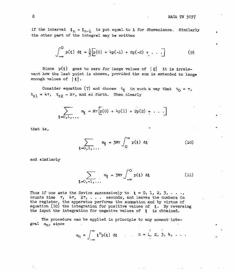
i s t o be measured. Using Simpson's ru le the in tegra l can be written a s the sum .

8 NACA TN 3037

if the in te rva l E n - En,l i s put equal..to 1 f o r C6nveGence. Similarly a

the other part of the in tegra l may be wri t ten

Since p ( ~ ) goes t o zero f o r large values of 1 1 it. is i r r e l e - vant how the last point i s chosen, provided the sum i s extended t o large enough values of ( E 1 .

Consider equation (7) and choose tE i n such a way t h a t to = r,

tk 1 = 4'3 tk2 = 27, and so for th . Then clear ly

- that is, -

and s h i l a r l y

Thus i f one se t s the device successively t o 6 = 0, 1, 2, 3, . . J

counts time T, 47, 27, . . . seconds, and leaves the numbers i n the reg is te r the apparatus performs the summation and by v i r tue of equation (101 the integration fo r posit3ve values of 5 . By reversing the input the integration f o r negative values of 5 is obtained.

The procedure can be applied in principle t o m y momen-tinte- g r a l %, since

MACA TN 3037

Now te is chosen as follows:

to = 0 tk1 = 4~(+l)~ ts = 2 ~ ( 5 ) ~ . . .

Thus

and thus

and

A procedure like this is sometimes convenient. Since the functions are smooth, not very many points are required to approximate the inte- grals very closely. It is also evident that this procedure could well be performed automatically if the additional apparatus were warranted.

Short Cuts

For some applica5ions it is possible to shorten the procedure very much by using a known form of p(5 ) . For example, assume that ~ ( t ) represents a velocity fluctuation u(t) in' isotropic turbulence. In this case one knows that p(5 ) is very nearly a Gaussian distribution. Thus :

i2 - - -

p(r) = P(o)~ 2-P

10

and hence

Thus

- - u25& ~2 = E l 2 - - 512.

P( 0) 2 log - 2 loi3 (k) p'(~1)

NACA TN 3037

-

and thus E 2 i s obtained as the r a t i o of'two measurements. Similarly - E 4 can be obtained.

Computation of Mean Values Using Multichannel Analyzer

Consider the mean value of the nth power of the input ~ ( t ) :

Now

so tha t

NACA TN 3037

and by equations (1) and (2)

Because of the factor . rn, the integrand becomes i n f i n i t e a t the l imi ts , d i n g it unsuitable f o r numerical evaluation. This d i f f i c u l t y can be overcome by transforming t o an in tegra l with respect t o the C-axis. Sp l i t t i ng the in tegra l in to two p a r t s about 5 = 0:

where F(O) = a . Integrating by parts :

The f i r s t two terms vanish a t the &its i f ~ ( n ) approaches zero exponentially or f a s t e r as E approaches minus in f in i ty . This require- ment is always s a t i s f i e d i f the mean value i s f i n i t e . Therefore

12 NACA TN 3037

The integrals are evaluated numerically by Simpson's rule, (see fig. 3. ) Since the main concern in turbulence work is distributions approaching a Gaussian form, the fourth moment of a Gaussian distribution was com- puted by Simpson's rule, using nine point^. The result deviated from the theoretical value by less than 1 percent.

In practice, the, normalization procedure

involves dividing the number of counts 9 in any register by the total number of pulses generated by the pulse generator during the iounting time Mg so that:

One can conveniently run the generator for 1 minute with a pulse rate . .

of 105 per minute, so that-

Finally, it may be called to mind once again that the exact posi- tion of 5 = 0 is not known beforehand. Using the fact that the first - moment of the distribution function is equal to zero (that is, V = 0)) the position of 'this axis may be determined. This procedure has proved more satisfactory than any in which one tries to set:the initial "zero" pulse amplitude to some known arbitraxy value with the accuracy required for cowuting mean odd powers.

DETAILS OF APPARATUS

Original Gate Circuit for p ( ~ )

The circuit diagrams of the elements are shown in figures 4 and 5. The block diagram is given in figure 6, which should be self-explanatory.

NACA TN 3037

The mixer w i l l be seen to ,be a twin t r iode normally running saturated through a c o m n anode load resistance. Strong negative gr id signals w i l l cut off the t r iodes, but a large anode s ignal w i l l appear only when both halves of the tube a r e cut off simultaneously. The small e f f ec t of one-half being cut off alone i s omitted i n the block diagram. It should be pointed out t h a t one-half of the f i r s t mixer receives a posi- t i v e square wave which causes gr id current t o flow, thereby building up a steady negative bias nearly equal t o the peak voltage of t h a t square wave, so tha t it considers i t s e H t o be receiving a negative input during the periods when t h i s posi t ive square wave i s absent. A s the 5 + d5 l i n e approaches the peak of the input signal, t h i s posi t ive square wave becomes of very short duration and it i s d i f f i c u l t f o r the mixer t o hold i t s b ias . I n operation the steps shown i n f igure 6 must be studied on an oscilloscope and levels adjusted, so t h a t the sundry effects , such as those mentioned above, do not in t e r f e re with the counting of the desired pulses.

The s ignal i s f i r s t amplified t o about a 100-volt peak, t o enable the gap t o be of. the order of a few vol t s and s t i l l be small compared with the peak amplitude. The Helipot A ( f ig . 4) adjusts the t r iggering point of the gate, t h a t is, E ; the two resistances B and C adjust the operating points of the two sides of the gate independently and hence s e t the gap width, t h a t i s , dE .

Adjustments a re made by studying the output of the en t i r e device .

on an oscilloscope, while a sine-wave signal i s being fed in. The poai- t i o n of A f o r 5 = 0, the width of the gap dE i n vol ts , and the ampli- f i ca t ion fac tor giving 5 or the se t t ing of A i n vol t s can be determined i n t h i s fashion.

Pulses can be generated i n any convenient manner, f o r example, by d i f fe rent ia t ing a square wave and suppressing the posi t ive pulses pro- duced, but f o r many applications it i s qui te good enough simply t o use a sine wave. The frequency was ordinari ly chosen to be 20'kilocycles per second, but d i f fe rent frequencies have been used.

The resu l t ing pulse sequences a re counted on a binary scalar counter feeding a mechanical reg is te r having a maximum r a t e of 60 per minute and capable of regis ter ing up t o lo4. The binary system i s standard pract ice and uses diode. coupling. The mechanical counter ( a ~ ~ c i o t r o n Specia l i t ies product) can be switched i n t o count every 25 t o 29 pulse by thpping onto the output of the f i f t h , s ixth, . . ., ninth stages of the binary scalar counter. This switching i s useful i n obtaining more counts on the reg is te r at low counting r a t e s ( i n preference t o reading the neon l i g h t of each stage and adding t o the r eg i s t e r reading) and may a lso be employed when integrating by Simpson's r u l e with the apparatus.

Multichannel Analyzer

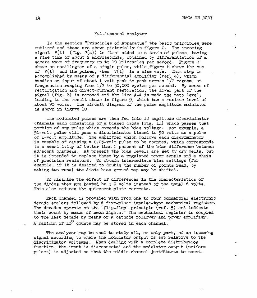
I n the sec t ion "Principles o f Apparatus" the basic principles were outlined and these a re shown p ic to r i a l ly i n f i g u r e 2 . The incoming signal ~ ( t ) ( f i g . 2(a) ) i s f i r s t added t o a t r a i n of pulses, having a r i s e time of about 2 microseconds, obtained-by d i f fe rent ia t ion of a square wave of frequency up t o 10 kilocycles per second. Figure 7 shows an oscillogrgm of a s ingle pulse, .while.Ngure 8 shows the sum of ~ ( t ) a n d t h e p u l s e s , when ~ ( t ) i s a s i n e w a v e . T h i s s t e p i s accomplished by means of a d i f f e ren t i a l amplifier ( r e f . G ) , which handles an input--of about 1 volt peak t o peak across 11/2 megohm, a t frequencies ranging from 1/2 t o 50,000 cycles per second. By means of rec t i f ica t ion and direct-current restoration, the Lower par t of the signal ( f i g . 8) is removed and the l i n e A-A i s made the zero level, leading t o the r e s u l t shown i n f igure 9, which has a, maximum l e v e l of about 90 vol ts . The c i r c u i t diagram of the pulse amplitude modulator is shown i n figure LO.

The modulated pulses a re then fed into 10 amplitude discriminator channels each consisting of a biased diode ( f i g . 11) which passes tha t portion of any pulse which exceeds the b ias voltage. For example, a 51-volt pulse w i l l pass a discriminator biased t o 50 vol ts as a pulse of 1-volt amplitude. The amplifier which follows each discriminator i s capable of causing a 0.05-volt pulse -t;o be counted, which corresponds t o a sens i t iv i ty of be t t e r than 1 percent of the bias difference between adjacent channels. A t present the bias levels a re s e t by dry ce l l s , but it i s intended t o replace these by a regulated power supply and a chain of precision res i s tors . To obtain intermediate b ias se t t ings ( fo r example, i f it i s desired t o double the number of points read, by W i n g two runs) the diode bias ground tap may be shif ted.

To minimize the e f f e c t o f differences i n the charact-eristics of the diodes they a re heated by 3.9 vol t s instead of the usual 6 vol t s . This a l so reduces the quiescent p l a t e currents.

Each channel i s provided with from one t o four commercial electronic decade scalars followed by R five-place impulse-type mechanical reg is te r . The decades operate on the "fl ip-flopu principle ( r e f . 5 ) and indicate the i r count by means of neon l i g h t r The mech&nical-register is coupled t o the l a s t decade by means of aca thode follower arid. power amplifier.

9 ,. A maximum of 10 counts m y be stored i n each channel.

The analyzer may be used t o study a l l , or only par t , of an incoming signal according t o where the modulator output is s e t re la t ive t o the discriminator voltages. When dealing with a c o q l e t e d is t r ibut ion function, the input i s disconnected and the modulator output (uniform pulses) i s adjusted so that the middle channel just-tarts t o count.

NACA TN 3037 15

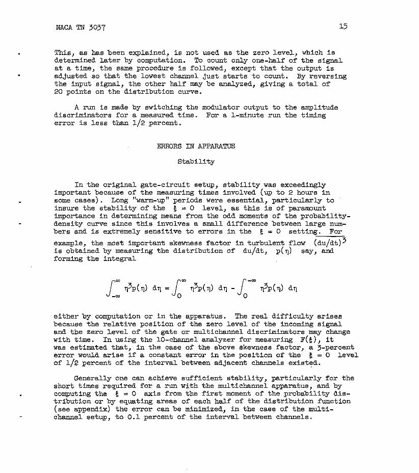
This, as has been explained, is not used as the zero level, which is determined later by computation. To count only one-half of the signal at a time, the same procedure is followed, except that the output is adjusted so that the lowest channel just starts to count. By reversing the input signal, the other half may be analyzed, giving a total of 20 points on the distribution curve.

A run is made by switching the modulator output to the amplitude discrbinators for a measured time. For a 1-minute run the timing error is less than 1/2 percent.

ERRORS I?J APPARATUS

Stability

In the original gate-circuit setup, stability was exceedingly important because of the measuring times involved (up to 2 hours in - some cases) . Long "warm-up" periods were essential, particuLarly to insure the stability of the 5 = 0 level, as this is of parmunt importance in determining means from the odd moments of the probability- - density curve since this involves a small difference between large num- bers and is extremely sensitive to errors in the 5 = 0 setting. For

example, the most important skewness factor in turbulent flow (du~dt)~ is obtained by measuring the distribution of du/dt, p(l) say, and forming the integral

either by computation or in the apparatus. The real difficulty arises because the relative position of the zero level of the incoming signal and the zero level of the gate or multichannel discriminators may change with time. In using the 10-channel analyzer for measuring F(s), it was estimated that, in the case of the above skewness factor, a 3-percent error would arise if a constant error in the position of the 5 = 0 level of 1/2 percent of the interval between adjacent channels existed.

Generally one can achieve sufficient stability, particularly for the short times required for a run with the multichannel apparatus, and by computing the 5 = 0 axis from the first moment of the probability dis- tribution or by equating areas of each half of the distribution function (see appendix) the error can be minimized, in the case of the multi- - channel setup, to 0.1 percent of the interval between channels.

Eysteresis . Any circuit designed to trigger at a certain voltage will exhibit a

certain amount of hybteresis. Some hysteresis is necessary for stability. In effect, the circuit triggers at one voltage when the input is increasing and at a slightly lower voltage when the input is decreasing. The effect of this imperfection can be reduced by increasing the voltage of the input signal. However, too large an input signal results in a very short time of transit through the gap, in the case of the original gate circuit, and the final output square waves becoqe distorted, ' d i n g it impossible to count properly. In the case of the multichannel analyzer, the use of

. biased diodes as discriminators has reduced hysteresis to a negligible amount.

Gap' Width in original Gate Circuit

The finite width of the gap does introduce a correction, which, - however, can be-esthted. If the gate width is equal to E, say, then

what is really measured is the quantity

and not p( S ) dg = p( k ) E . For a small a, however, one evidently has

and for a known distribution the correction can be evaluated. For example, if p(S ) is nearly Gaussian

Ordinarily measurements have t o be taken up t o values of 5 of

the order of . Hence the maximum er ror near the outer edges of

the dis tr ibut ion is of the order

This e r ror may be appreciable i f f a i r l y large gate widths a re used. However, the er rors i n the dimensionless r a t i o s of moments of p ( ~ ) , namely, the skewness and f la tness factors, a r e much smaller and fo r the most par t negligible. For exan~ple, the er rors in the f la tness factors can be evaluated from

The f la tness fac tor f is

The fac tor f obtained from the measured d is t r ibut ion can be wri t ten

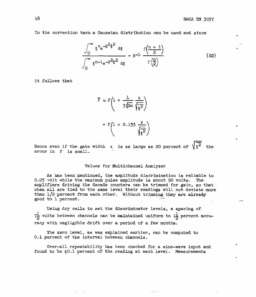
In the correction term a Gaussian d is t r ibut ion can be used and since

it follows t h a t

Hence even i f the gate width E is as large as 20 percent of &? the e r ror i n f i s small.

Values f o r Multichannel Analyzer

A s has been mentioned, the amplitude discrimination is r e l i ab le t o 0.05 vol t while the maximum pulse amplitude is about 90 vol t s . The amplifiers driving the decade counters can be t r i m e d for gain, so t h a t when a l l a r e t i e d t o the same l eve l t h e i r readings w i l l not deviate more than 1/2 gercent from each other. Without trimming they a re already good t o 1 percent. .-

Using dry c e l l s t o s e t the discriminator levels, a spacing of 1 vol t s between channels can be maintained uniform t o I- percent accu- 7~ 2

racy with negligible d r i f e o v e r a period of a few mgnths.

The zero level , a s was explained ea r l i e r , can be computed t o 0.1 percent of the in te rva l between channels.

Over-all repeatabi l i ty has been checked fo r a sine-wave input and found t o be f O . l percent of the reading a t each level . Measurements

NACA TN 3037 19

of du/dt i n a turbulent a i r stream gave the following sca t t e r of the mean values computed from consecutive 1-minute runs:

- x k 1 percent ~2 % k2 percent

- - v3 z t3 percent v4 % f 4 percent

Main Improvement Introduced by 10-Channel Setup

It should now be clear tha t , whereas the gate c i r c u i t d r a w s i t s information from selected narrow bands of the incoming signal, the 10-channel device u t i l i z e s the whole s ignal . This can, of course, be done with the gate c i r c u i t by using only one t r igger c i r c u i t and su i t - ably rearranging the block diagram of f igure 6, but, because of the long time involved i n measuring, the s t a b i l i t y requirements become pro- h ib i t ive . Operat- 10 channels as a p(S) device with large intervals - defeats the advantage of using p ( ~ ) , namely t h a t moments can be com- puted i n the apparatus by sui table t M n g (see sect ion "Obtaining Mean values") , since the correction outlined above i n "Gap Width i n Original - Gate ~ i r c u i t " has t o be applied and therefore leads t o computation work. It w i l l be realized, too, t h a t measuring F(E) instead of p(E) leads t o cer ta in simplifications i n c i r cu i t ry since each channel has t o dis- t inguish only whether each pulse does o r does not r i s e above i t s b ias level . These were the considerations which led t o the adoption of the present arrangement.

Other schemes w i l l be found i n references 6 t o 9, but the present arrangement is designed f o r r e l a t ive ly high counting r a t e s .

SAMPLE APPLICATIONS

Sine Wave

The multichannel analyzer was checked out on a s ine wave (190 cycles per second) . The re su l t s f o r one-half of the s ignal a r e shown i n f ig - ure 12, together with the theore t ica l r e su l t , and show close agreement.

Isotropic Turbulence

Figure 13 shows the r e su l t s of measurements. of p(E) with the gate . c i rcu i t , f o r the a x i a l veloci ty d is t r ibut ion i n isotropic turbulence - behind. a gr id. The Gaussian d is t r ibut ion is shown fo r comparison.

20 NACA TN 3037

Agreement is good and confirms observat-ions by others, especially Townsend. Skewness and f la tness factors a re shown i n the tab le i n the next section.

Figure 14 shows ~ ( 5 ) f o r the same quantity under prac t ica l ly the same conditions, a s measured on the 10-channel analyzer.

Isotropic Turbulence, du/dt and d2u/dt2

Fi?y e 15 presents the r e su l t s of measurements of the dis t r ibu- t i o n p ) of the velocity derivative du/dt, using the gate, while figure 1 presents the d is t r ibut ion function F(?) f o r the same quan- t i t y and prac t ica l ly the same conditions. The interest ing f a c t here is the asymmetry of the d i ~ t r i b u t i o n as first demonstrated by Townsend ( r e f . 3) . From the d is t r ibut ion p( the mean values can be computed. However, i n order t o compute the odd moments, t h a t is, du3/dt f o r example, one has t o be very sure about the or ig in of the coordinate 7, t ha t is, about the zero posit ion. Since a s tat ionary process is dea l t with here, evidently

Hence one has t o obtain first the "center of gravity" of the dis t r ibu- t i o n and then compute the moments about this point. For the even moments t h i s is not very Important and a s l igh t shift of the zero point amounts t o a negligible er ror . The de ta i l s of the-computation f o r the case of the 10-channel analyzer a re given i n the appendix. -

The skewness and f la tness factors obtained are--shown in the following tables . Included a l so is the fac tor C defined by

fo r u and du/dt, respectively. Results for d2u/bt2 using the . 10-channel analyzer a re also given. ( ~ l s o see f i g . 17.)

The following tables give a comparison of measurements behind a b

turbulence gr id with a mesh s ize M = 3/4 inch; denotes the Remolds number based on the mesh s ize, and x/M denotes the illmensionless his- tance from the gr id position.

With gate c i r cu i t , % = 8,100, and x/M = 62:

With 10-channel analyzer, % = 11,000, and x/M = 50:

S f C

These values agree well with Townsend's measurements. Towmend gives fo r the skewness factor of du/dt, S .= -0.39, but the measure- ments plotted, fo r exanrple i n f igure 8 of reference 10, range between 0.39 and 0.50 a t l e a s t . The f la tness factor of u found here is some- what l e s s than Townsend's value of 2.9 ( ref . 11) . Hence the present measurements do not agree as well with a Gauss& distribution, fo r which f = 3. The same resul t i s borne out by C which should be

Jn/2 f o r a Gaussian dis tr ibut ion. Again the dis tr ibut ion of u does give a noticeable difference. The symmetry of the u dis tr ibut ion is, however, well shown by S, which i s zero t o a close approximation.

Jo in t Probability Density , ) From Zero Counts *

During the investigation of the poss ib i l i t i e s of using the number

of zeros of u ( t ) t o determine ( d ~ / d t ) ~ (or h) it w a s necessary t o assume tha t u ( t ) and du/dt were s t a t i s t i c a l l y independent; t h a t is,

22 NACA TN 3037

it was assumed tha t p(5, rl) = pO(f )p1(rl) . Using the present. device with •

the or iginal gate c i r cu i t itn-is possible t o check how closely t h i s assump-

t i o n agrees with the fac ts , t ha t is, horr accurately ( d ~ / d t ) ~ can be 1

measured from the zero counts.

The number N(S ) of 5 .values of u ( t ) , t ha t i s , the number of times per second that u ( t ) passes g , is given by ( r e f s . 1 and 12)

Denote the probabili ty dis t r ibut ion of u( t ) , t h a n s , the average time tha t u ( t ) spends between 5 and 5 + d l , as P o ( ~ ) d l . EYidently

p0(6) Can be written

Taking the r a t i o N/P~ one has

Equation (24) describes the following fac ts : po(E) d5 denotes the

time t which u ( t ) spends between 5 and 5 + dg, and M(E) gives the number of passages through f per uni t time; hence the r a t i o

NACA TN 3037 23

gives the average time of a s ingle passage. Hence the average absolute slope of a passage is given by

I n general, 1 dl1 depend upon 5; however, if p(5 ,i) = pO(5)pl(~)

then

which is independent of 5 . This re la t ion means tha t , if the probabil i t ies of u and du/dt are independent, the absolute mean of du/dt is the same a t every point of the t race u ( t ) .

An example f o r which t h i s is evidently not t rue is a s-le harmonic wave of angular frequency cu; t ha t i s

u ( t ) = s i n c u t

Here, N(5 ) = U/YC is of course independent of 5 . However, the time spent between 5 and 5 + d5 increases with 5 and hence

expressing the f a c t that the mean absolute slope I has i t s maximum a t = 0 and decreases t o zero as 5 j 1 .

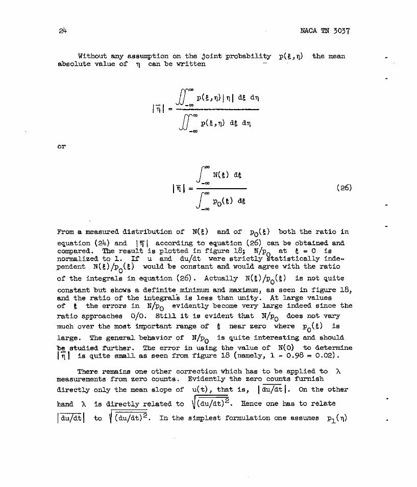
Without any assumption on the joint probabili ty p(E,v) the mean absolute value of 11 can be wri t ten -

From a llheasured d is t r ibut ion of N(S) and of po(e) both the r a t i o i n

equation (24) and 1 Fj 1 according t o equation (26) can be obtained and compared. The r e su l t i s plot ted i n f igure 18; nIp0 at 6 = 0 i a normalized t o 1. If u and du/dt were s t r i c t l y s t a t i s t i c a l l y inde- pendent N(6) /po(E) would be constant and would agree with the r a t i o

of the integrals in equation (26) . Actually N(S) IPO(k) is not qui te

constant but shows a def in i te minimum and naaximum, as seen in figure 18, and the r a t i o of the integrals is l e s s than unfty. A t large values of 5 the errors i n N / ~ ~ evidently become very large indeed since the r a t i o approaches 010. S t i l l it is evident tha t N / P ~ does not vary much over the most important range of E near zero where pO(5) is

large. The general behavior of is qui te interest ing and should be studied fur ther . The error i n using the value of ~ ( 0 ) to determine 1 1 is qui te small as seen from figure 18 (namely, I - 0.98 = 0.02) .

There remains one other correction which.has t o be- applied t o h measurements from zero counts. Evidently the zero counts furnish

d i r ec t ly only the mean slope of u ( t ) , that is, I du/dt 1 . On the other

hand h is d i r ec t ly re la ted t o \ . Hence one has t o r e l a t e 1 ' -

I du/dt I t o (du/dt) '. I n the simplest formulation one assumes pl( 11)

NACA TN 3037

t o be Gaussian and then the r a t i o

Now pl(q) is not qui te Gaussian and hence the re la t ion between I du/dt 1 and I- k i l l d i f f e r from w. L e t

Then the formula eq loyed i n the measurement of h by counting zeros should read

where U denotes the mean speed. For C = the formula evidently reduces t o the one used in reference 1

The fac tor C w a s evaluated from the measured d is t r ibut ion as has been shown i n the preceding table:

and hence

26 - NACA 'I% 3037

Consequently i n h2 about 6 percent e r ror r e su l t s from the use of the - simple formula, equation ( 2 7 ) . Thus h would come out-- too large using equation (27) . This i s an er ror in the r igh t - -direction since the measure- - ments of references 1 and 13 consistently give too large values of h as calculated from equation ( 2 7 ) . The correction due t o the weak s t a t i s t i c a l dependency of u and du/dt is, however, i n the other direct ion and the combined ef fec t of these two errors i s insufficient-to explain the d i f - ferences found i n reference 13 between A from zero counts and A measured independently. It seems more l ike ly that these differences can be .traced t o small systematic e r rors i n the equipment, f o r example, insuf- f ic ient resolution.

Vortex St ree t

Figure 19 shows the dis t r ibut ion funct-ion, by the 10-channel analyzer, obtained i n a vortex s t r e e t behind a cylinder a t a Reynolds number of 100. The hot-wire output was a very s tab le , almost tr iangular wave. A t rue t r i ang-~ la r wave would give a s t raight- l ine d is t r ibut ion function. The rounded peaks of the actual wave form give deviations from a s t ra ight l i n e near the ends, where the d is t r ibut ion curves inward as i n the dis- t r ibut ion function fo r the s ine wave. This work was done in conjunction with the study of wakes ( r e f . 14) .

California I n s t i t u t e of Technology, Pasadena, Calif . , September 29, 1952.

NACA TN 3037

APPENDIX

CALCULATION OF POSITION OF 5 = 0 AXIS

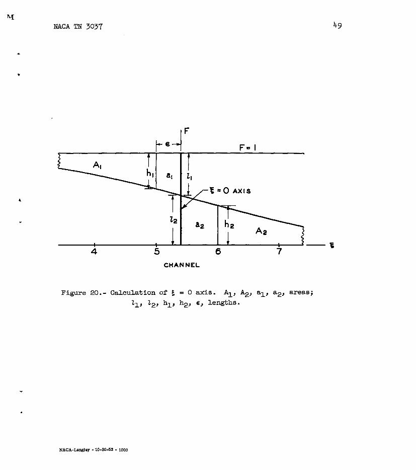
Figure 20 is to be used in conjunction with this discussion of the calculation of the 5 = 0 axis. The distance E of the zero axis from channel 5 is found by the following method.

For zero average value of the input signal,

where A1 and A2 are determined fr6m the data by use of Simpson's rule.

. The c u e between channels 5 and 6 can usually be accurately approxi-

mated by a straight line. Therefore, al and a2 are computed by using the trapezoidal rule as follows:

But,

28 . . . . -

Substituting ,

2(a2 - a 3 = h, + 1 - h1 + (hl + h, - 1 ) ~ - (hl + $)E - E

Therefore,

NACA TN 3037

REFERENCES

1. L i e p m , H. W.: Die Anwendung eines Satzes iiber d ie Nullstellen s tochs t i sche r Funktionen auf Turbulenzmessungen. Helvetica Physica Acta, vol. 22, no. 2, Mar. 18, 1949, pp. '119-126.

2. Robinson, Martin S.: A Ten Channel S t a t i s t i c a l Analyzer f o r Use i n Turbulence Research. Aero. Eng. Thesis, C.I .T. , 1952.

3. Townsend, A. A , : The Measurement of Double and Triple Correlation Derivatixes in Isotropic Turbulence. Proc. Cambridge Phil . Soc., vol. 43, p t . 4, ~ c t . 1947, pp. 560-570.

4. Seely, Sanuel: Electron-Tube Circuits. F i r s t ed., McGraw-Hill Book Co., k c . , 1950.

5. Chance, Britton, e t al . , eds.: Waveforms. F i r s t ed., McGraw-Hill Book Co., Inc., 1949.

6 . Parsons, J. H.: Electronic Classifying, Catalog-, and Counting Systems. Proc. Ins t . Radio Engs., vol. 37, no. 5 , May 1949, pp. 564-568.

7. Westcott, C. H., and Hanna, G. C. : A Pulse Amplitude Analyzer f o r Nuclear Research Using Pretreated Pulses. Rev. Sci. Ins t r . , vol. 20, no. 3, M a r . 1949, pp. 181-188.

8. Freundlich, H. F., Hinks, E. P., and Ozeroff, W. J.: A Pqlse Analyzer for Nuclear Research. Rev. Sci. Instr., vol. 18, no:2, Feb. 1947, pp. 90-100.

9. Wells, F. H.: A Fast Amplitude Discriminator and Scale-of-Ten Counting Unit for Nuclear Work. Jour. Sci. Ins t r . , vol. 29, no. 4, Apr. 1952, pp. 111-115.

10. Bat.chelor, G . K., and Townsend, A. A.: Decay of Vorticity i n Iso- t ropic Turbulence. Proc . Roy. Soc . o on don) , ser . A, vol. 190, no. 1023, Sept. 9, 1947, pp. 534-550.

11. Batchelor, G . K . , and Townsend, A. A.: The Nature of Turbulent Mt ion a t Large Wave-Nurtibers . Proc. Roy. Soc. ondo don) , ser . A, voi. 199, no. 1057, Oct. 25, 1949, pp. 238-255.

12. Rice, S. 0.: Mathematical Analysis of Random Noise. The Bell System Tech. Jour., vol. 23, no. 3, July1944, pp. 282-332; vol . 24, no. 1, Jan. 1945, pp. 46-108.

3 0 NACA TN 3037

13. Liepmann, R. W., Laufer, J., and Liepmann, Kate: On the Spectrum of Isotropic Turbulence. NACA TN 2473, 1951.

14. Roshko, A . : On the Development of Turbulent W&es From Vortex Streets . Ph. D . Thesis, C.I.T., 1952. ( ~ l s o available as NACA TN 2913.)

NACA TN 3037

(a) Fluctuating voltage.

(b) Square-wave signal from gate c i rcui t .

(c) Signal from pulse generator.

(d) Signal produced by mixing signals from gate and pulse-generat or c i rcui ts .

Figure 1.- Principle of gate circuit .

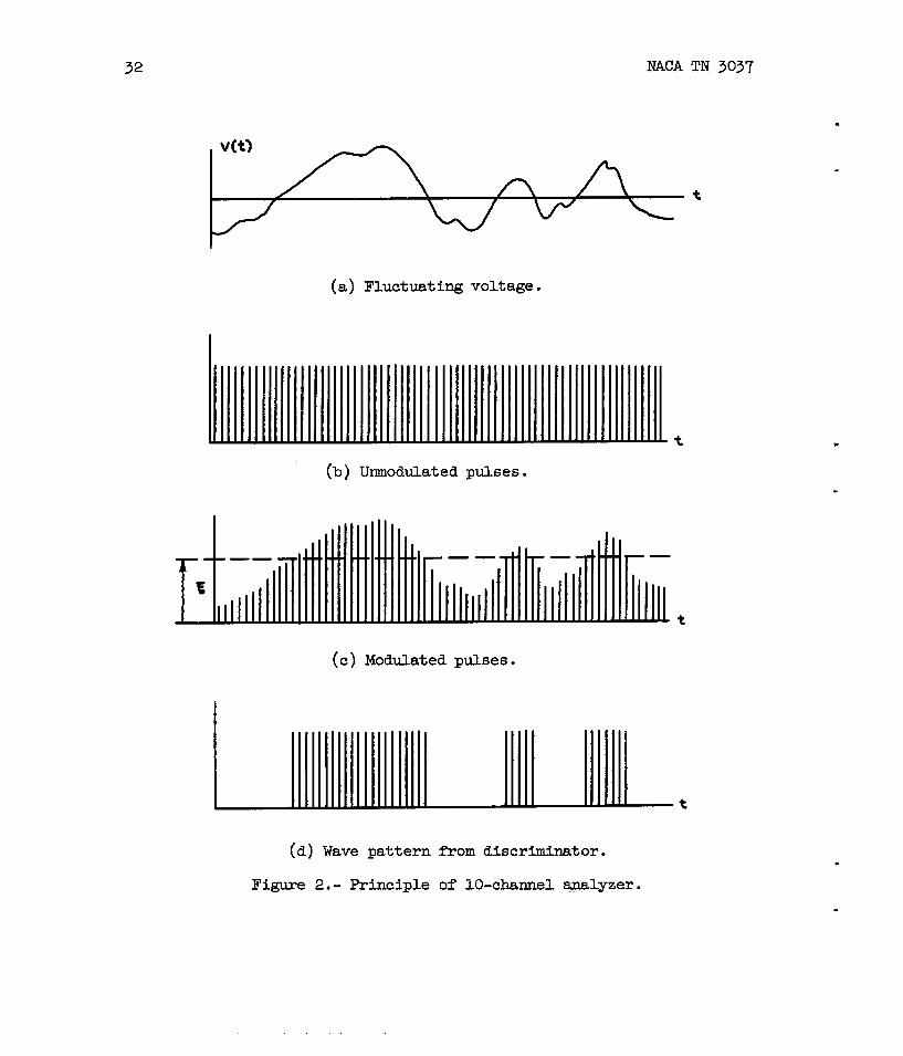
( a ) Fluctuating voltage.

(b) Unmodulated pulses.

(c) Modulated pulses.

(d) Wave pat tern f r o m discriminator.

Figure 2.- Principle of 10-channel aplyzer.

NACA TN 3037

REGION OF INTEGRATION IN EQUATION (15)

Figure 3. - Typical. d i s t r ibut ion function.

NACA TN 3037

POTENTIOMETER FOR SETTING VALUES

@ TRIGGERING ADJUSTMENT FOR CIRCUIT (1 )

@ TRIGGERING ADJUSTMENT FOR ClRCuIT(2)

@ OUTPUT EQUALIZATION CONTROL

O METER T o ENABLE CURRENT , N O T O BE KEPT CONSTANT

Figwe 4. - Double-trigger c i r cu i t of gate. (K indicates thousand; WW, wire-wound re s i s to r . )

NACA TN 3037

-- -- INPUT (I) INPUT (2)

a-0 OUTPUT

l NVERTER MIXER

Figure 5. - Circuit diagrams of inverter and mixer. (K indicates thousand. )

a INPUT

1- OUTPUT

PULSES

Figure 6. - Block &gram of apparatus.

NACA TN 3037

L-80245 Figure 7.- V i e w of a single pulse.

NACA TN 3037

L-80246 Figure 8. - Different ia l amplifier output f o r a sine-wave input.

L-80247 Figure 9.- Modulator output f o r a sine-wave input.

Figure LO.- C F r c u i t diagram of pulse amplitude modulator.

NACA TN 3037

MODULATOR 043 .5 MEG 31+

COUNTER V

AMPLIFIER

Figure 11. - Pulse height discriminator.

Figure 12.- Distribution function f o r a sine wave.

Figure U.- Di s t r i ba ion of u i n isotropic turbulence (corrected f o r gap d d t h ) . %=8,100, ~ / ~ = 6 2 ; ~ = 0 . 9 4 4 m , S = O . W , f= .2 .36 .

Figure 14. - Distribution fbmt ion f o r u ( t ) In isotropic turbulence. % = 11,000, X/M = 50, M = 1.68 centimeters; C = 0.9m, s = 0.006, f = 2.77.

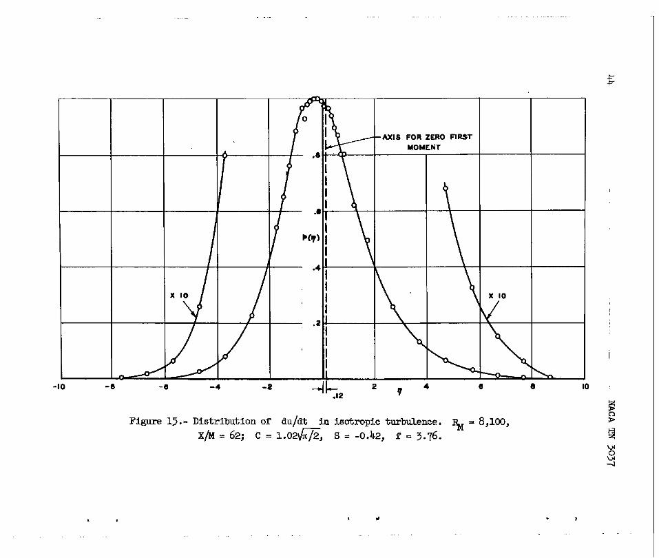
Figure 15 .- Distribution of du/dt in isotropic turbulence. % = 8J1COJ x/M = 62; C = 1 . 0 2 f i J S = -0.42, f = 3.76.

Figure 16. - Distribution function fo r du/dt in isotropic turbulence. % = U,OOO, X / ~ I = 30, M = 1.68 centimeters; C = 0.984@, S = -0.439, f = 3.80.

H

Figure 17. - Distribution function for d%/at2 in isotropic turbulence. z

% = ~ , w o , x/M = 50, M = 1.68 centimeters; C = l.dc@, 8 = 0.031, w o W

f =: 4.59. -a

Figure 18.- Plot of N(s)/P~(s).

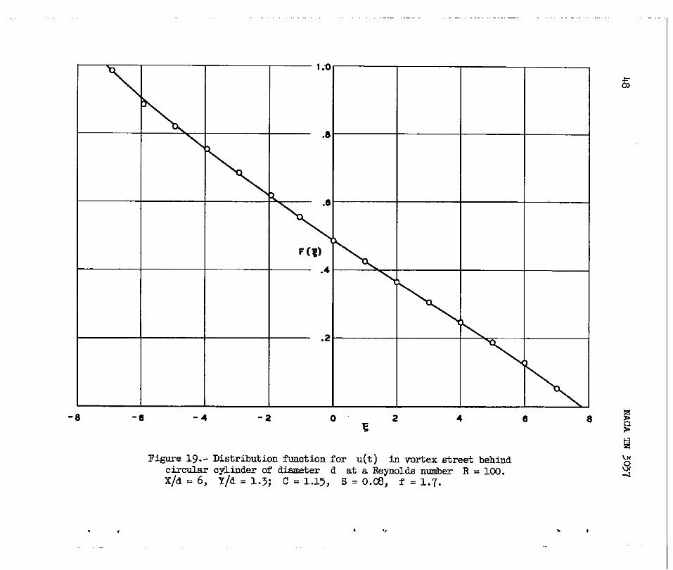
Pi- 19.- Distribution function for u ( t ) in vortex s t r ee t behind circular cylinder of diameter d a t a Reynolds nuniber R = 100. x / a = 6 , y / d = l . j ; c=1.15, s=o.c$, f = i . 7 .

NACA TN 3037

CHANNEL

Figure 20.- Calculation of 5 = 0 axis. A1, A2, al, a2, areas;

zl, z2, hl, h2, c , lengths*