Cramer-Rao Sensitivity Limits for Astronomical Interferometry

218 J. Opt. Soc. Am. A/Vol. 20, No. 2 /February 2003 Jonas Zmuidzinas

Cramer–Rao sensitivity limits forastronomical instruments:

implications for interferometer design

Jonas Zmuidzinas

Division of Physics, Mathematics, and Astronomy, California Institute Institute of Technology, 320-47 Pasadena,California 91125

Received April 24, 2002; revised manuscript received July 23, 2002; accepted September 25, 2002

Multiple-telescope interferometry for high-angular-resolution astronomical imaging in the optical–IR–far-IRbands is currently a topic of great scientific interest. The fundamentals that govern the sensitivity of direct-detection instruments and interferometers are reviewed, and the rigorous sensitivity limits imposed by theCramer–Rao theorem are discussed. Numerical calculations of the Cramer–Rao limit are carried out for asimple example, and the results are used to support the argument that interferometers that have more com-pact instantaneous beam patterns are more sensitive, since they extract more spatial information from eachdetected photon. This argument favors arrays with a larger number of telescopes, and it favors all-on-onebeam-combining methods as compared with pairwise combination. © 2003 Optical Society of America

OCIS codes: 030.4280, 030.5260, 030.5290, 110.4280, 120.6200, 270.5290, 350.1270.

1. INTRODUCTIONAstronomical spatial interferometry, which is the tech-nique of combining the radiation gathered by severalseparated telescopes, is of great current interest becauseof the scientific potential of very-high-angular-resolutionobservations, combined with numerous technological ad-vances that now make interferometry feasible atoptical–IR wavelengths. As a result, this field is very ac-tive, and serious investments are being made: Numer-ous ground-based facilities are in development, large ar-rays are being discussed, and ambitious space missionsare being considered. Detailed reviews of this field,which describe the scientific motivation and results, tech-nical challenges and approaches, and existing andplanned facilities and which contain extensive bibliogra-phies, have been made recently.1,2 Additional informa-tion is readily available.3

Of course, interferometry is very well developed at ra-dio wavelengths, at which large arrays of telescopes, suchas the National Radio Astronomy Observatory Very LargeArray (NRAO VLA),4 routinely provide high-angular-resolution synthetic aperture imaging. Ground-based in-terferometry at optical wavelengths is inherently moredifficult owing to the limitations imposed by atmosphericphase fluctuations; dealing with these fluctuations is per-haps the key issue for ground-based systems and providesstrong motivation to consider interferometry in space.As a result, NASA is pursuing the Space InterferometryMission,5 an optical astrometric interferometer with a10-m baseline, scheduled for launch at the end of the de-cade. The Space Interferometry Mission will perform awide range of science, including searches for extrasolarplanets as well as synthetic aperture imaging of the cen-ters of galaxies. Another important advantage of spaceinterferometry is the unobstructed transmission and lowbackground over the entire IR–far-IR–submillimeterspectrum. Looking further into the future, IR interfer-

1084-7529/2003/020218-16$15.00 ©

ometers are being considered for missions such as the Ter-restrial Planet Finder6 and Darwin,7 which have the am-bitious goal of detecting and characterizing Earth-likeplanets around nearby stars. Direct-detection space in-terferometers at very long (far-IR–submillimeter) wave-lengths that use cold telescopes have also been proposed,such as the NASA Submillimeter Probe of the Evolutionof Cosmic Structure and Space Infrared InterferometricTelescope (SPECS/SPIRIT) concepts.8–10 Such interfer-ometers would give the angular resolution needed tobreak through the spatial confusion limit,11 which be-comes severe at these long wavelengths, and would allowa detailed study of the properties of the newly discoveredclass of submillimeter-luminous, dusty galaxies at highredshifts.12–14

In spite of this high level of activity, it appears that im-portant design considerations for optical interferometersare not yet resolved. One major issue is the number oftelescopes that should be used; another issue is themethod of beam combination. Of course, various practi-cal constraints may limit the range of design options; forinstance, it is likely to be important to minimize thenumber of telescopes for a space interferometer. Al-though a number of papers have addressed these variousissues,15–24 there appears to be no general consensus onwhich design approaches give the best sensitivity or evenif there is much difference between them.1 It is essentialto have a full understanding of the fundamental issuesthat determine the sensitivity of optical interferometers;advancing that understanding is the goal of this paper.We will therefore ignore important technical issues, suchas the methods used to deal with atmospheric fluctua-tions, mechanical and thermal perturbations, detectornoise, etc., and discuss only interferometers with nearlyideal characteristics.

Our approach will focus on the instantaneous (not syn-thesized) angular response function or beam pattern as-

2003 Optical Society of America

Jonas Zmuidzinas Vol. 20, No. 2 /February 2003 /J. Opt. Soc. Am. A 219

sociated with a given detector that receives the light gath-ered by the interferometer. We will argue on generalgrounds, supported by the Cramer–Rao lower bound onthe uncertainty of statistical inference, that it is impor-tant to make the instantaneous angular response func-tion as compact as possible in order to extract the maxi-mum amount of spatial information from each detectedphoton. This argument favors certain interferometer de-signs over others. For instance, pairwise beam combina-tion in which the light from T telescopes is split and in-terfered on T(T 2 1)/2 detectors (one detector perbaseline), which is essentially the approach adopted forradio interferometry, is, in general, less sensitive fordirect-detection interferometric imaging than schemes inwhich the light from all T telescopes is coherently com-bined onto the detectors. The reason for this is that theangular response functions are less compact for the caseof baseline pair combination, and each photon detectedprovides less information about the spatial structure ofthe source. This distinction vanishes for the radio case,in which one is dealing with amplified signals that havehigh occupation numbers for the photon modes, and sophoton bunching plays an important role. The connec-tions and distinctions between the optical and the radiocases will be discussed in more detail in a future paper.25

The structure of the paper is as follows. Sections 2–5are devoted to giving a rigorous definition of the photon-detection probability matrix of an arbitrary astronomicalinstrument, such as an interferometer, in terms of electro-magnetic scattering matrices. The formalism describedin these sections is quite powerful and allows us to handleany interferometer configuration or beam-combiningmethod. Many of the key results described in these sec-tions are well known and will likely be familiar. How-ever, the use of scattering matrices and photon-detectionprobability matrices to describe astronomical instrumentsand interferometers is not common and is therefore cov-ered in some depth.

The key mathematical results are described in Section6. There we discuss the Cramer–Rao sensitivity bound,as well as two techniques (maximum likelihood and leastsquares) that can be used to obtain the source intensitydistribution from the observed photon counts; the overallgoal is to argue that the Cramer–Rao lower bound actu-ally gives a good estimate of the instrument performance.We also show that the only instruments that can achieveideal sensitivity are those that do not mix up photonsfrom different spatial or spectral channels. Unfortu-nately, such instruments are difficult to build; interferom-eters do, in fact, mix up photons spatially (and spectrally,in some cases).

To demonstrate the consequences of a nonideal re-sponse, in Section 7 we present the results of a numericalcalculation of the Cramer–Rao bound for the simple butillustrative case of one-dimensional interferometer ar-rays. To do this, we draw on the material presented inSections 2–6. Here we demonstrate that arrays with alarger number of telescopes are superior and that N-waybeam combining is superior to two-way combining. Thepaper closes with comments on these results and indi-cates areas for future research.

2. SCATTERING MATRIX DESCRIPTION OFOPTICAL SYSTEMSThe response of any electromagnetic system, such as acollection of optical elements (mirrors, lenses, etc., but notdetectors), may be described by a classical scattering ma-trix S. Scattering matrices are common in electricalengineering,26,27 in which they are used to describe linearN-port circuits:

bi 5 (j

Sijaj . (1)

The indices 1 < i, j < N label the ports. A set of Ntransmission lines attached to the ports carries incomingwaves with amplitudes ai and outgoing waves with am-plitudes bi . The standard practice is to normalize theseamplitudes to give simple expressions for the power car-ried by the waves; for instance, the total incident power isQ inc 5 ( iuaiu2. With this choice of normalization, it isstraightforward to show that a lossless circuit has a uni-tary scattering matrix, SS† 5 I (here I is the identity ma-trix). Reciprocity, which has its roots in time-reversalsymmetry and applies to most passive circuits, impliesthat ST 5 S. When the wave amplitudes are expressedin terms of voltages and currents at the ports, the scatter-ing matrix S may be related to more familiar quantitiessuch as the impedance matrix Z. Finally, we note that(classical) noise can be treated very naturally within theframework of scattering matrix theory.26,28–30 The exten-sion to include quantum effects, such as photon-countingstatistics, is straightforward.25

We can apply the scattering matrix concept to charac-terize an optical system, such as the collection of tele-scopes and beam-combining optics that make up an inter-ferometer. This approach was developed for antennaproblems during the World War II radar effort31 and isparticularly convenient at radio wavelengths, since it al-lows circuit and antenna concepts to be treated in a uni-fied fashion. Although scattering matrices are fre-quently applied to antenna problems,32,33 they are notoften used to describe optical systems (though they dofind occasional use34). Scattering matrices are very use-ful for describing guided-mode optics, which are, in fact,of substantial interest for astronomical interferome-try.35,36 Scattering matrices are also very well suited forproblems involving the quantum-mechanical nature ofthe radiation field, such as photon-counting statistics, be-cause one directly deals with the modes of the radiationfield. For these reasons, we adopt the scattering matrixapproach. To make the paper reasonably self-contained,and to establish our notation, we will review this ap-proach in detail.

We begin by describing the radiation field in terms ofincoming and outgoing plane waves. For simplicity, wewill continue to use a classical description for the electro-magnetic field; it is straightforward to adapt our formal-ism to the case of a quantum electromagnetic field.25 As-suming a time-harmonic exp(1jvt) time dependence, theelectric field of the incoming wave arriving at the tele-scope system (or antenna) can be expressed as


Einc~r! 5A2h0

lE dVa~V!exp@1jkn~V! • r#. (2)

Here a(V) represents the amplitude and polarization dis-tribution of the incoming plane waves, l is the free-spacewavelength, and h0 5 377V is the free-space impedance.As usual, V represents the polar angles (u, f) with respectto the chosen coordinate system; the unit vector n(V)5 z cos u 1 sin u (x cos f 1 y sin f ) describes the direc-tion from which a plane-wave component is arriving.Similarly, the outgoing wave can be expressed as

Eout~r! 5A2h0

lE dVb~V!exp@2jkn~V! • r#. (3)

The normalization is again chosen to give simple expres-sions for power, for instance,

Q inc 5 E dVua~V!u2. (4)

In the usual case of incoherent light emitted by astro-nomical sources, the wave amplitudes can be consideredto be random quantities with certain statistical proper-ties.

An antenna is usually thought of as having one or morewell-defined ports, or terminals, that one can attach toother circuits, such as an amplifier. In the case of a radiotelescope, the terminal may well be the output waveguideof a feedhorn. The situation is a little more subtle for thecase of an optical telescope system, in which the light isfocused directly on the bare pixels of a detector array,such as a CCD. [In reality, the distinction between opti-cal and radio techniques is blurring. For instance, theintroduction of single-mode optical fibers for collectingand transporting light from the focus of a telescope iscompletely analogous to the use of radio feedhorns andwaveguides, and bare pixel detector arrays find use evenat very long (submillimeter) wavelengths.] We can imag-ine describing the radiation incident on a given detectorpixel, which we label a, in terms of a modal expansion.At the detector surface, these spatial modes may be con-strained to have a nonzero amplitude only over the regionoccupied by the pixel (for pixel sizes exceeding ;l, thisconstraint makes the modes for different pixels orthogo-nal, which simplifies the form of the scattering matrix).The ith such mode for pixel a has incoming wave ampli-tudes aia and outgoing wave amplitudes bia , which weassume have the usual power normalization. We will de-fine the terms ‘‘incoming’’ and ‘‘outgoing’’ in reference tothe telescope system rather than the detector pixels, sothat the light gathered by the telescope system that ar-rives at the detectors is characterized by the amplitudebia . Assuming perfect absorption by the detector, thepower absorbed can be expressed as

Qa 5 (i

ubiau2. (5)

Imperfect absorption by the detector (quantum efficiencybelow unity), as well as varying sensitivities to the differ-ent spatial modes, can be incorporated into the definitionof the scattering matrix of the optical system, which we

discuss below. In the case of a system designed fordiffraction-limited imaging, most of the light absorbed bythe detector will be contained in a single mode (or twomodes, for polarization-insensitive detectors).

The telescopes and associated optical system (e.g.,beam-combining optics) can be characterized by a gener-alized scattering operator S. This operator acts on a Hil-bert space consisting of vectors of the form

a 5 Fa~V!

aiaG , (6)

where a(V) is square integrable. The operator S can bepartitioned into four blocks:

S 5 F S~scat! S~rec!

S~trans! S ~refl!G . (7)

The first block, S(scat)(V, V8), describes the scattering ofan incoming plane wave arriving from V8 to an outgoingplane wave traveling toward V. The script font remindsus that this is a 3 3 3 matrix to account for polarization.The second and third blocks are off diagonal: Sia

(rec)(V8)describes the (vector) receiving antenna pattern for thedetector pixel mode ia, and Sjb

(trans)(V) describes thetransmitting antenna pattern. The fourth block is an or-dinary matrix, Siajb

(refl) , that represents the scattering (re-flection) of the optical system between the various detec-tor pixel modes. The meaning of these quantitiesbecomes clear when we write expressions for the outgoingwaves in terms of the incoming waves:

b~V! 5 E dV8S~scat!~V, V8!a~V8! 1 (jb

Sjb~trans!~V!ajb ,

(8)

bia 5 E dV8Sia~rec!~V8! • a~V8! 1 (

jbSiajb

~refl!ajb .

(9)

Assuming that the optical system contains only recip-rocal elements (e.g., no Faraday rotation isolators), weknow that the scattering operator must equal its trans-pose. This implies that the transmitting and receivingpatterns are the same:

Sia~trans!~V! 5 Sia

~rec!~V!, (10)

which is the well-known reciprocity theorem for anten-nas. In addition, the radiation scattering operator obeys

S ~scat!~V, V8! 5 @S ~scat!#T~V8, V!, (11)

and the pixel-to-pixel scattering matrix is reciprocal,S (refl) 5 @S (refl)#T.

The output power emanating from a passive opticalsystem cannot exceed the input power, which imposes animportant constraint on the scattering operator: I2 S†S must be nonnegative definite. Combined withthe reciprocity theorem, this can be used to demonstratethat the following matrix must also be nonnegative defi-nite:


Mia, jb 5 d ia, jb 2 E dV@Sia~rec!~V!#* • Sjb

~rec!~V!

2 (kg

@Skg,id~refl! #* Skg, jb

~refl! . (12)

In particular, the diagonal elements must be nonnegative,which implies

E dVuSia~rec!~V!u2 < 1 2 (

jbuSjbia

~refl!u2 < 1. (13)

Thus the overall normalization of the receiving patternsis not arbitrary. If we demand that the optical system belossless and if the detector modes are perfectly coupled@S (refl) 5 0#, the receiving patterns must be orthonormal:

E dV@Sia~rec!~V!#* • Sjb

~rec!~V! 5 d ia, jb . (14)

We now calculate the power received by any detectorpixel. We assume that any imperfect absorption (includ-ing reflection) associated with the detector pixel has beenincorporated into the definition of S. Furthermore, weassume that the detectors do not radiate into the opticalsystem, so that aia 5 0. (The detectors are usually oper-ated at a temperature low enough that the thermal radia-tion they emit is negligible.) The power absorbed bypixel a is

Qa 5 (i

ubiau2 5 (i

U E dVSia~rec!~V! • a~V!U2

. (15)

3. ASTRONOMICAL SOURCESAstronomical sources emit radiation that is spatially andtemporally incoherent. This means that we should re-gard the amplitude a(V, n) at frequency n as a complexrandom variable with mean zero and with a correlationfunction of the form

^aq~V, n!aq8* ~V8, n8!& 5 Aqq8~V, n!d ~V 2 V8!

3 d ~n 2 n8!. (16)

Here aq(V, n) 5 eq* (V) • a(V, n) and q, q8 P $1, 2% arevector (polarization) indices, corresponding to two ortho-normal polarization vectors eq(V), each orthogonal to thepropagation direction n(V). We note that the plane-wave expansion of the incoming field is unique in thesense that the correlation function is diagonal in the spa-tial variable. Had we chosen some other modal represen-tation, e.g., a vector spherical harmonic expansion, theamplitude correlation matrix, in general, would not be di-agonal in the mode indices.

The physical interpretation of Aqq8(V, n) follows froma calculation of the flux F(p, s, n), the power per unitbandwidth per unit area, in a given polarization p that isincident on a surface with normal s:

F~p, s, n! 51

l2 (qq8

E dVn~V! • s

3 F p* • eq~V!Aqq8~V, n!eq8* ~V! • p

u1 2 n~V! • pu2 G .

(17)

For sources occupying a small solid angle near zenith ( s5 z), the total flux for both polarizations simplifies to

Ftotal~n! 51

l2 (qE dVAqq~V, n!. (18)

Thus Aqq(V, n)l22 is the specific intensity (flux per unitsolid angle) arriving from the direction V in polarizationeq(V). For unpolarized emission, we can write

Aqq8~V, n! 5 hn n~V, n!dqq8 , (19)

where n(V, n) is the mean photon occupation number.This simplifies to Aqq 5 kBT for a blackbody in theRayleigh–Jeans limit.

4. RESPONSE OF AN OPTICAL SYSTEM TOAN ASTRONOMICAL SOURCEThe average power per unit bandwidth received from anastronomical source by a detector pixel can be calculatedwith Eqs. (15) and (16):

^Qa~n!& 5 (qq8

E dVAqq8~V, n!H(i

@ eq • Sia~rec!~V, n!#

3 @Sia~rec!~V, n! • eq8#* J . (20)

For an unpolarized source, Aqq8(V, n) 5 A(V, n) dqq8 ,this reduces to

^Qa~n!& 5 E dVA~V, n!Ra~V, n!, (21)

where we have defined the angular response function cor-responding to this detector:

Ra~V, n! 5 (i

uSia~rec!~V, n!u2. (22)

For a source that has uniform brightness over the areasampled by the response function Ra(V, n), the power re-ceived is ^Qa(n)& 5 ma(n) A(V, n), where the effectivenumber of modes ma (spatial and polarization) coupled tothe detector is defined as

ma~n! 5 E dVRa~V, n!. (23)

According to inequality (13), ma(n) < ( i1, and so ma(n)cannot exceed the number of modes received by the detec-tor that are illuminated by the telescope.

For the opposite extreme, we take the case of a pointsource located at Vp. The power received by one detectoris

^Qa~n!& 512 F~n!l2Ra~Vp, n!, (24)


where F(n) is the flux (both polarizations) of the pointsource. On the other hand, for a telescope system withtotal collecting area Atel , the power collected by all thedetectors cannot exceed F(n) Atel . Thus

(a

Ra~Vp, n! <2Atel

l2 . (25)

Since the response functions are all positive, each indi-vidual response function must also obey this inequality.Therefore if the response function Ra(V, n) has a flat-topshape extending over a solid angle DVa , the effectivenumber of modes obeys

ma <2AtelDVa

l2 . (26)

This statement is often called the antenna theorem; onecannot increase the number of modes coupled to a givendetector without simultaneously broadening the angularresponse function.

Inequality (25) suggests that we renormalize our re-sponse functions:

ra~V, n! 5l2

2AtelRa~V, n!, (27)

so that they obey

(a

ra~V, n! < 1. (28)

The power received by a detector [Eq. (21)] can now be ex-pressed as

^Qa~n!& 52Atel

l2 E dVA~V, n!ra~V, n!. (29)

We can discretize this integral by splitting the source intosmall patches or ‘‘pixels’’ centered at positions Vs , allow-ing each patch to have a different size DVs and assumingthat the source has uniform intensity across each patch:

A~V, n! 5 (s

A~Vs , n!Us~V!, (30)

where the indicator function Us(V) has a value of unityover the patch DVs and is zero otherwise [some sort of re-striction on the form of A(V, n) is necessary, since a dis-crete set of data cannot uniquely determine a function ofa continuous variable]. This gives

^Qa~n!& 5 (s

2DVs Atel

l2 A~Vs , n!ra~Vs , n!, (31)

where the average of the response function over patch s is

ra~Vs , n! 51

DVsE

DVs

dVra~V, n!. (32)

Finally, using this result along with A(V, n)5 hn n(V, n) [Eq. (19)], we arrive at a very simple andilluminating expression for the average number of pho-tons detected in a unit bandwidth during an integrationtime t:

^Na& 5 E dn(s

^N~Vs , n!&ra~Vs , n!, (33)

where

^N~Vs , n!& 5 t2DVsAtel

l2 n~Vs , n! (34)

is just the maximum average number of photons (per unitbandwidth) that a single-aperture telescope with area Atelcould detect in a time t from the solid-angle patch DVs .The interpretation of the normalized response function issimple: ra(V, n) is the probability that a photon of fre-quency n that was emitted from position V and was col-lected by the instrument is actually detected by detectora. The total probability for detection is at most unity, ac-cording to inequality (28).

If we wish, we can take the additional step of discretiz-ing the frequency integral into spectral channels Dn f ,which leads to

^Na& 5 (s,f

^N~Vs , n f!&ra~Vs , n f!, (35)

where the maximum average number of detectable pho-tons in frequency channel Dn f is

^N~Vs , n f!& 5 tDn f

2DVsAtel

l2 n~Vs , n f! (36)

and the response function is now also averaged over fre-quency:

ra~Vs , n f! 51

DVsDn fE

Dnf

dnEDVs

dVra~V, n!. (37)

Equations (35) and (36) tell us that the response of anyphoton direct-detection instrument, regardless of spectralor spatial resolution, whether single telescope or interfer-ometer, etc., can be reduced to a probability matrix pac .Here, for simplicity, the combined spatial–spectral chan-nel index c replaces both indices s and f:

pac 5 ra~Vs , n f!. (38)

This matrix describes the probability of a photon, whichwas emitted by the source in some spatial–spectral chan-nel c and is collected by the instrument, to be absorbed ina given detector a. Let

lc 5 ^N~Vs , n f!& (39)

represent the mean number of incident photons fromchannel c arriving at the instrument. The mean numberma of photons detected by detector a is given by

ma 5 ^Na& 5 (c

paclc . (40)

A few comments can be made about the properties ofthe probability matrix P.

1. From inequality (28) we have

(a

pac < 1, (41)


so that the mean number of photons detected cannot ex-ceed the mean number of incident photons, (ama

< (clc .2. Since all elements are nonnegative, we also must

have0 < pac < 1. (42)

3. The dimensions of the matrix are Ndetec 3 Nchan .Thus the rank of the probability matrix, r(P), obeysr(P) < Nchan . Here Ndetec is the number of detectors andNchan is the number of spatial–spectral channels.

4. If we wish to determine uniquely the source inten-sity distribution lc in Nchan spatial–spectral channels, weshould require P to have full rank: r(P) 5 Nchan . Inparticular, this condition implies Ndetec > Nchan .

These properties and their implications will be discussedin more detail in Section 6.

5. RESPONSE OF SINGLE-MODEINTERFEROMETERSSection 4 gives us the tools to rigorously calculate thephoton-detection probability matrix for an interferometer.The primary reason for constructing interferometers is toobtain high spatial resolution; the overall field of view isoften a secondary concern. Thus it is interesting to ex-amine the case of an interferometer in which each tele-scope collects light from a single diffraction-limited beam,which sets the field of view. For simplicity, we will as-sume that the interferometer consists of T identical tele-scopes, each with area A1 . The total collecting area isAT 5 TA1 . The receiving pattern corresponding to thesingle diffraction-limited beam of telescope t (where t5 1 ... T) will be denoted by St

(rec)(V, n), following ourestablished notation. These receiving patterns are as-sumed to be identical, apart from the fact that the tele-scopes are located at different positions. We denote thetelescope positions with respect to an arbitrary (but com-mon) origin using the displacement vectors rt . The re-ceiving patterns can then be written as

St~rec!~V, n! 5 exp@1ikn~V! • rt#S~rec!~V, n!. (43)

Here the pattern S(rec)(V, n) denotes the receiving pat-tern of a telescope located at the origin. Each of thesetelescopes produces a single-mode output beam, describedby an outgoing wave amplitude bt :

bt~n! 5 E dVSt~rec!~V, n! • a~V, n!. (44)

The receiving patterns from different telescopes t Þ t8are orthogonal to a high degree,

E dV@St~rec!~V, n!#* • St8

~rec!~V, n!

5 E dVuS~rec!~V, n!u2 exp@2ikn~V! • ~rt 2 rt8!#

' 0, (45)

because of the oscillations of the exponential factor. Thismeans that the telescopes are not coupled significantly(as can happen for closely packed antenna arrays), and it

is therefore possible to achieve nearly perfect coupling tothe single-mode outputs. For this case, the telescope pat-terns are orthonormal [see Eq. (14)]. If necessary, cou-pling losses can be accounted for in the beam combiner,which we introduce next.

The purpose of the beam combiner is to interfere thelight from different telescopes before it is detected.There are various ways to do this: The telescopes can becombined in pairs, analogous to the way that radio-correlation interferometers operate, or all the light fromthe telescopes can be interfered simultaneously, as is donein Fizeau interferometry. Beam combination is a key is-sue for interferometer design. We can describe any typeof beam-combining scheme using a scattering matrixS (comb). This matrix tells us how the wave amplitudes btfrom the single-mode telescope feeds are coupled to thewave amplitudes bia arriving at the detectors:

bia~n! 5 (t

Sia,t~comb!bt~n!. (46)

By combining Eqs. (44) and (46), we have

bia~n! 5 (t

Sia,t~comb!~n!St

~rec!~V, n! • a~V, n!. (47)

For astronomical sources, we are interested in the re-sponse function Ra(V, n) [see Eq. (22)], which in this caseis

Ra~V, n! 5 (i

U(t

Sia,t~comb!~n!St

~rec!~V, n!U2

. (48)

These response functions must obey the inequality ex-pressed in inequality (25), with the factor of 2 removed,since we are collecting only a single mode (single polariza-tion). For single-mode interferometers, we would define

ra~V, n! 5l2

ATRa~V, n!, (49)

and we would also omit the corresponding factor of 2 inEq. (36). Using Eqs. (38), (48), and (49), we can calculatethe photon-detection probability matrix pac for an inter-ferometer. Although we have assumed identical tele-scopes, it is straightforward to generalize our expressionsto include heterogeneous arrays.

Aperture synthesis imaging refers to the technique ofrepeatedly observing a given astronomical source withdifferent configurations of the telescopes that form an in-terferometer. This is a standard technique in radio as-tronomy; interferometers are constructed with multiplepossible positions or stations for each telescope, and thetelescopes are physically moved to these different sta-tions. In addition, aperture synthesis imaging usuallyrelies on the rotation of the Earth, which, in essence, ro-tates the interferometer as a function of time with respectto the astronomical source. The source is assumed not tovary over the time taken to gather the aperture synthesisobservations.

It is quite straightforward to take into account multipletelescope configurations within our formalism. Thephoton-detection probability matrix pac;a depends on thetelescope configuration, which we label by the discrete in-dex a (the different orientations produced by Earth rota-tion may be binned). We can replace the indices a and a


with a combined index b. If there are Nconfig telescopeconfigurations and the interferometer has Ndetec physicaldetectors, then b will take on NconfigNdetec different values,and we can consider b to be an index for a set of virtualdetectors. This allows us to define a new photon-detection probability matrix that describes the entire setof aperture synthesis observations:

pbc 5 pac;awa , (50)

where the weighting factor wa is simply the fraction ofthe total observing time that was spent in configuration a,

wa 5Ta

(a8

Ta8

, (51)

where Ta is the time spent observing in configuration a.The properties of the photon-detection probability matrixdiscussed at the end of Section 4 also hold for the case ofaperture synthesis (with Ndetec reinterpreted as the num-ber of virtual detectors).

6. POISSON DECONVOLUTION PROBLEMAND THE CRAMER–RAO BOUNDA. Introduction and OverviewWe have seen that any optical instrument, including aninterferometer used for aperture synthesis imaging, maybe described by a photon-detection probability matrix P,with elements pac . According to Eq. (40), this matrix re-lates the mean photon counts ma registered by the detec-tors to the source distribution lc . Some sort of inversionprocedure must be applied to obtain an estimate lc of thesource distribution from the observed counts Na . Howwell can this deconvolution be done? What is the noise inthe deconvolved image (or spectrum)? The answer to thisquestion depends on

• the statistics of the photon counts,• the deconvolution method that is used,• the nature of the probability matrix P.

We will assume that the photon counts have indepen-dent Poisson distributions (as we discuss below).Clearly, we should expect in all cases that the variance ofDlc 5 lc 2 lc obey the inequality

sc2 5 ^~Dlc!

2& > lc , (52)

since the number of photons emitted from the source inchannel c has a Poisson distribution with mean lc . Thisinequality will be derived, and the conditions on P thatare necessary and sufficient to achieve this limit will begiven.

A wide variety of deconvolution methods have beenproposed2; in this paper we will discuss two: a simplelinear least-squares (LS) method and the maximum-likelihood (ML) method. In general, the ML method issuperior, but it is nonlinear and is therefore more difficultto compute and analyze. Since the LS method is not op-timal, its performance provides only an upper bound to

the sensitivity. However, in the important special case inwhich all detectors receive the same photon flux (ma allequal), we will see that the LS upper bound actually co-incides with the Cramer–Rao lower bound (described be-low), and therefore both give the actual sensitivity.

The Cramer–Rao theorem gives a rigorous lower boundfor the sensitivity that holds for any deconvolutionmethod. We will use this result to derive inequality (52)and to show that the ideal sensitivity limit can beachieved only if the instrument does not allow photonsfrom different spatial–spectral channels to arrive at thesame detector. In other words, an ideal instrument doesnot mix up photons from different channels, and aphoton-detection event can be unambiguously assigned tothe appropriate spatial–spectral channel. Consequently,such an instrument would achieve the lower bound onsensitivity given by inequality (52). The definition of anideal instrument is given more precisely below. Unfortu-nately, interferometers, in general, do not obey our defini-tion and do mix up photons spatially (and spectrally) andtherefore cannot achieve the ideal sensitivity limit.

The Poisson deconvolution problem arises in manyother contexts, such as positron-emission tomography formedical imaging37; as a result, there is extensive litera-ture on this subject. In fact, iterative ML algorithms forPoisson deconvolution do exist, e.g., the Richardson–Lucyor the expectation maximization algorithm (see the re-view by Molina et al.38 and the references therein). Theexistence of ML algorithms is important, since the noiseperformance of the ML method is guaranteed to asymp-totically approach the Cramer–Rao bound in the limit ofhigh signal-to-noise ratio (SNR). However, in cases thatthe likelihood function has multiple local maxima, theCramer–Rao bound often fails to give a realistic estimateof the achievable sensitivity and does not give even aqualitative description of how the sensitivity varies withthe SNR. This occurs because the estimation problem isambiguous—the various local maxima represent alter-nate possible solutions. The Cramer–Rao bound be-comes useful only when the SNR is large enough so that aunique solution can be chosen among these various possi-bilities. Examples include time delay and bearing esti-mation problems39–41; in such cases, other techniquessuch as the Ziv–Zakai bound must be used. Fortunately,this situation does not occur for the problem we are study-ing. We shall see that if the rank of the probability ma-trix is equal to the number of spatial–spectral channels@r(P) 5 Nchan#, then a finite Cramer–Rao bound exists,the LS deconvolution also exists, and the likelihood func-tion has a single maximum that defines the unique MLdeconvolution. Conversely, if r(P) , Nchan , a finiteCramer–Rao bound does not exist, the LS deconvolutionmay fail, and the ML method may yield a degenerate sub-space of possible solutions instead of a single unique so-lution.

Thus a finite Cramer–Rao bound should correspond tothe actual sensitivity of an astronomical instrument or in-terferometer for bright objects or for long integrations;one simply needs to ensure that the photon counts arelarge, Na @ 1. The Cramer–Rao bound can thereforeprovide a useful tool for quantitatively comparing thesensitivity of various interferometer design options.


B. Poisson StatisticsIt is well established that the photon counts registered bythe detectors in an optical instrument follow statisticallyindependent Poisson distributions, so that the fluctua-tions of the counts in different detectors are uncorrelated.To be more precise, this situation holds for the case ofthermal emission (from the source, the atmosphere, thetelescope, etc.) in which the mean photon occupationnumbers of the modes incident on the detectors are low,n ! 1. In the high occupancy limit, n @ 1, photonbunching becomes important in that it changes the count-ing statistics and can introduce correlations among thedetectors. We will discuss only the first case, n ! 1,which applies to most astronomical observations at opti-cal and infrared wavelengths.

C. Definition of an Ideal InstrumentWe define an ideal instrument in terms of its probabilitymatrix pac , which is required to obey the condition

pac pac8 5 0 (53)

for all detectors a and for all c8 Þ c. This condition sim-ply states that if pac Þ 0, then pac8 5 0. In words, if adetector receives photons from the spatial–spectral chan-nel c, it cannot receive photons from some other channelc8. This allows us to group the detectors into disjointsets that may be indexed by the channel that the detec-tors respond to. Furthermore, we require that the totaldetection probability for any channel c be unity: (a pac5 1. It is evident that such an instrument can achievethe ideal sensitivity limit set by inequality (52); to esti-mate the source intensity in channel c, we simply sum thephoton counts from the set of detectors responding tochannel c. By considering this set of detectors as anequivalent single detector, one can readily see that anyideal instrument is equivalent to an instrument that hasa probability matrix equal to the identity matrix, pac5 dac .

The spatial and spectral resolution of an ideal instru-ment would therefore be set by our definition of thespatial–spectral channels c, which is, in principle, arbi-trary. Do ideal instruments really exist, at least in prin-ciple? Achieving the required spectral resolution withoutmixing up photons spectrally is not a fundamental diffi-culty; all one needs is a large enough grating. Achievingthe required spatial resolution without mixing up photonsspatially is a more subtle issue, since the parameters lcrefer to a fixed telescope collecting area, according to thedefinition in Eqs. (36) and (39). However, we can use asingle-aperture telescope, with a diameter sufficientlylarge to achieve the spatial resolution required, as long aswe reduce the transmission (i.e., use a neutral-density fil-ter) to keep the effective collecting area (and the param-eters lc) constant. Of course, doing so would be foolish;this argument serves only as an existence proof.

D. Cramer–Rao Sensitivity LimitThe Cramer–Rao theorem provides a strict lower limit forthe variance of a quantity that is estimated from a set ofnoisy measurements. This theorem can be applied to de-termine the minimum noise in the determination of theintensity in some spatial–spectral channel by use of an

instrument with a nonideal response, one whose probabil-ity matrix differs from the identity matrix. The HubbleSpace Telescope, whose initial point-spread function suf-fered from spherical aberration that has since been cor-rected, provides a particularly well-known example of thesubstantial sensitivity degradation that occurs as a resultof a nonideal response, which cannot be undone by imagerestoration techniques such as the maximum-entropyalgorithm.42 In fact, the Cramer–Rao limit was appliedto exactly this situation by Jakobsen et al.43 TheCramer–Rao theorem has also been used to evaluatesimilar information loss effects in other imaging prob-lems, for instance, gamma-ray imaging in nuclearmedicine.44

We start by quickly reviewing the Cramer–Raotheorem.45–47 Let us consider an experiment that deliv-ers a set of measurements, denoted by the vector x, butthat has scatter that is due to measurement noise. Themeasurement process can be described by a probabilitydistribution f(xuu) to obtain a result x. Here the vector urepresents the unknown parameters or quantities thatthe experiment is sensitive to, such as the source inten-sity distribution in our case. The usual goal is to deter-mine one or more of these parameters from the measureddata, say, u i . To do this, we must construct some estima-tor u i(x) that uses the measured data vector x to estimateu i . For simplicity, we assume that this estimator is un-biased; the results could be generalized to include bias.First, we define the matrix

Mij~u! 5 K ] ln f

]u i

] ln f

]u jL

5 E dxf~xuu!] ln f~xuu!

]u i

] ln f~xuu!

]u j. (54)

This is known as the Fisher information matrix and issymmetric and nonnegative definite. In fact, it is posi-tive definite, unless there is some linear combination ofparameters u i that the function f(xuu) is completely inde-pendent of, in which case we should reparameterize toeliminate that linear combination. Thus we assume Mhas an inverse, M21, which is also positive definite. Fora detailed analysis of the case in which the Fisher infor-mation matrix is singular, we refer the reader to a recentpaper by Stoica and Marzetta.48

The Cramer–Rao theorem states that C > M21, whereC is the covariance matrix of the estimators, Cij 5 ^( u i

2 u i)( u j 2 u j)&, and the matrix inequality is understoodto mean that C 2 M21 is nonnegative definite. In par-ticular, the diagonal elements give

s i2 5 ^~ u i 2 u i!

2& > ~M21!ii . (55)

A weaker limit can also be given:

s i2 > ~M21!ii > ~Mii!

21. (56)

The second (weaker) limit can be obtained by consideringthe case in which all other parameters are known exceptfor u i .


We now apply this to the photon-detection problem.The detector counts have independent Poisson distribu-tions:

f~Nul! 5 )a

maNa

Na!exp~2ma!, (57)

so

] ln f

]lc5 (

aS 2pac 1

Na pac

maD , (58)

Mcc8~l! 5 K ] ln f

]lc

] ln f

]lc8L 5 (

a

pac pac8

ma

5 (a

pac pac8

(c9

pac9lc9

, (59)

by virtue of ^Na Na8& 5 mama8 1 madaa8 . The Cramer–Rao sensitivity limit for channel c is

sc2 > ~M21!cc . (60)

Equation (59) and inequality (60) are key results, sincethey give us a quantitative way to set lower limits to thesensitivity of optical instruments. Alternatively, forsome purposes we may wish to use the weaker bound,sc

2 > (Mcc)21, which is the result quoted by Jakobsen

et al.43:

sc2 > F(

a

pac2

(c8

pac8lc8G 21

. (61)

It is easy to verify that either form gives sc2 5 lc in the

case of an ideal instrument, for which pac 5 dac . How-ever, we note that although the Cramer–Rao bound givenby inequality (60) is asymptotically achievable by the MLmethod, this is not true, in general, for the weaker bound.

These sensitivity limits depend on the values of lc , i.e.,the structure of the source. For the case of a pointsource located in channel c, inequality (61) gives sc

2

5 lc ((a pac)21 > lc ; the equality holds if all the pho-

tons are detected. The sensitivity limit given by thestronger Cramer–Rao bound [inequality (60)] is typicallyonly somewhat worse than this. The reason that thepoint-source sensitivity does not vary much with the in-strument response is that we are simply summing all thephotons counted by all the detectors; it does not mattermuch how the photons are distributed among the detec-tors. Thus calculations that only compare the sensitivi-ties of interferometers to point sources do not tell thewhole story.

It is illuminating to write Eq. (59) with matrix nota-tion:

M 5 PTG21P, (62)

where G 5 diag (m1 , m2 ,...) is a diagonal matrix. Fromthis expression, it is evident that the Fisher informationmatrix will be singular if the probability matrix P doesnot have full rank @r(P) , Nchan#.

It may appear that Eq. (62) presents a mathematicaldifficulty for the case of an ideal instrument observing apoint source, for which ma 5 0 for the off-source channels.A similar situation may also occur for nonideal instru-ments. However, one can imagine adding a low-levelbackground to the point source, so that now ma 5 e forthe off-source channels. The Fisher information matrixM is now well defined and can be inverted to obtain theCramer–Rao bound. Finally, the limit e → 0 can betaken.

E. Sensitivity Bound and Ideal InstrumentsWe now prove the sensitivity bound given in inequality(52) and show that only ideal instruments can actuallyachieve this limit. For some channel c, the weaker boundstates that

1

sc2 < Mcc 5 (

aPDc

pac2

ma

, (63)

where Dc 5 $au pac Þ 0%. Now

ma 5 (c8

pac8lc8 > paclc > 0, (64)

since all the terms in the sum are nonnegative. Thus

1

sc2 < (

aPDc

pac2

paclc5 (

aPDc

pac

lc<

1

lc, (65)

since (a pac < 1. This proves inequality (52). The con-ditions necessary to actually achieve this limit are evi-dent from the derivation: ma 5 paclc and (a pac 5 1.Since the source distribution lc is, in general, arbitrary,the first condition can be met only if pac8 5 0 for all c8Þ c. Thus the instrument must be an ideal instrument.We have therefore shown that only ideal instruments can(and do) achieve the sensitivity bound given by inequality(52).

F. Maximum-Likelihood DeconvolutionDeconvolution that uses the ML method is desirable,since the performance of the ML method is guaranteed toasymptotically approach the Cramer–Rao bound in thehigh SNR limit. Apart from a constant, the logarithm ofthe likelihood function for some estimate m of the meancount rate is [see Eq. (57)]:

ln f 5 (a

~Na ln ma 2 ma!. (66)

The goal of the ML method is to find a source distributionl that maximizes this function, where m 5 Pl. In gen-eral, we would seek the solution by setting the gradient tozero, ] ln f/]lc 5 0. However, the case in which Na 5 0for one or more detectors must be treated with care. Thedifficulty may be illustrated by first considering ln f to bea function of m directly. The maximum of this function isunique and occurs at ma 5 Na , and, in fact, ] ln f/]ma

5 21 for the detectors that have Na 5 0. The problemis that the maximum occurs at the boundary of the physi-cally acceptable region ma > 0. We can remedy thisproblem by making all detector counts nonzero, replacing


Na 5 0 with Na 5 e, where e ! 1. We then proceed tofind the ML solution using calculus; at the end, we takethe limit e → 0.

We therefore assume that Na . 0 for all detectors.The local maxima of the likelihood function must thenobey [see Eq. (58)]

] ln f

]lc

5 (a

pacS 21 1Na

maD 5 0 (67)

or, in matrix notation, PTv 5 0, where the components ofthe vector v are va 5 21 1 Na /ma . Thus v must be inthe null space of PT, which is the annihilator of the rangeof P. If there are Ndetec detectors and P has rank r(P), vis constrained to lie in a subspace of dimension Ndetec2 r(P). In addition, m must lie in the range of P, asm 5 Pl, which gives r(P) additional constraints. Over-all, we would get Ndetec constraint equations for v, whichcould be solved to yield the local maxima of the likelihoodfunction. However, since some of the constraints applylinearly to v and others apply linearly to m, the combinedset of equations are, in fact, nonlinear. As mentionedearlier, iterative algorithms for finding the solution(s) doexist.

We now demonstrate that, in general, there is only asingle local maximum of the likelihood function. Sup-pose instead that there were two distinct local maxima,corresponding to two different source distributions l (a)

and l (b). We can write m (a) 5 Pl (a) and m (b) 5 Pl (b)

and introduce the vectors v (a) and v (b), defined by theircomponents

va~a ! 5 21 1

Na

ma~a !

, (68)

and similarly for va(b) . Since these correspond to local

maxima, we know that we must have PTv (a) 5 PTv (b)

5 0, which tells us that both v (a) and v (b) must lie in theannihilator of the range of P. Since m (a) and m (b) lie inthe range of P, v (a) and v (b) must each be orthogonal toboth m (a) and m (b):

(a

ma~a !va

~a ! 5 (a

ma~b !va

~b ! 5 0, (69)

(a

ma~a !va

~b ! 5 (a

ma~b !va

~a ! 5 0. (70)

These conditions tell us that

(a

ma~a ! 5 (

ama

~b ! 5 (a

Na (71)

and also that

(a

NaF ma~a !

ma~b !

2 1G 5 (a

NaF ma~b !

ma~a !

2 1G 5 0. (72)

Define xa 5 ma(a)/ma

(b) > 0. Adding the equations aboveyields

(a

Nag~xa! 5 0, (73)

where g(x) 5 x 2 2 1 1/x. Now, the function g(x) has asingle minimum in the domain x > 0, located at x 5 1,and g(1) 5 0. Since Na . 0 and g(x) > 0, we must ac-tually have g(xa) 5 0 and so all xa 5 1, and thereforema

(a) 5 ma(b) . Thus Pl (a) 5 Pl (b). If P has full rank

@r(P) 5 Nchan#, we can conclude that l (a) 5 l (b), and so,in fact, there is only a single local maximum, and the MLdeconvolution is unique. If P does not have full rank, thesolution is ambiguous, and l (a) 5 l (b) 1 l, where l can beany vector in the null space of P. As discussed above, theFisher information matrix will be singular in this situa-tion, so the calculation of the Cramer–Rao bound will fail.Also, LS deconvolution will fail, since PTP will not havean inverse (see below).

G. Least-Squares DeconvolutionTo obtain a simpler (but suboptimal) linear method, wecould attempt to set v 5 0, which would give

ma 5 (c

paclc 5 Na . (74)

Since, in general, Ndetec . r, this system of linear equa-tions overconstrains l but may be solved in a LS sense.Another way of explaining this is that the vector m mustlie in the range of P, but, in general, the vector N does not.The LS algorithm is obtained by first projecting N into therange of P and then solving the resulting linear systemfor l:

l~LS! 5 ~PTP !21PTN. (75)

In general, PTP is symmetric and nonnegative definite.In fact, it is positive definite and has an inverse if andonly if P has full rank @r(P) 5 Nchan#. Thus the exis-tence of a finite Cramer–Rao bound guarantees both thatthe LS deconvolution exists and that the likelihood func-tion has a single maximum.

Because the LS deconvolution is linear, it is straightfor-ward to calculate its bias and its noise performance. Infact, the LS method is unbiased, since

^l~LS!& 5 ~PTP !21PTm 5 ~PTP !21PTPl 5 l. (76)

The covariance matrix of the LS deconvolution is given by

C ~LS! 5 ^DlLS~DlLS!T& 5 ~PTP !21PTGP~PTP !21,(77)

where G 5 diag(m1 , m2 ,...), as defined earlier. Since theLS method is not optimal, in general, this covariance ma-trix can be used to establish an upper bound to the sensi-tivity, to complement the Cramer–Rao lower bound.

In the case that ma 5 m are all equal, G 5 mI, we seethat the covariance matrix simplifies to

C ~LS! 5 m~PTP !21. (78)

Meanwhile, the Fisher information matrix [Eq. (62)] forthis case is M 5 m21PTP, so, in fact, the performance ofLS deconvolution achieves the Cramer–Rao bound. Thisis admittedly a special case. However, it may often occurin practice, at least approximately, e.g., for a uniformsource or when the photon counts are dominated by the


contribution of a uniform background such as thermalemission from the atmosphere or the telescopes.

Another interesting special case occurs when the prob-ability matrix P is square and has full rank, r(P)5 Nchan . Under these conditions, P can be inverted, andone can show that the LS and ML estimators are, in fact,the same:

l~LS! 5 l~ML! 5 P21N. (79)

Also, both estimators achieve the Cramer–Rao bound.

H. Interferometry, Aperture Synthesis, and theCramer–Rao BoundAstronomical aperture synthesis observations often donot obtain enough information to uniquely determine thesource intensity distribution (map) at the desired resolu-tion. In other words, the condition r(P) , Nchan applies,and so a finite Cramer–Rao bound does not exist. Insuch cases, a linear or nonlinear regularization method(such as the maximum-entropy method) may be appliedto select a single representative map that has certain de-sirable characteristics (e.g., smoothness, positivity) out ofthe infinite set of maps that are consistent with the mea-sured data.

What good is the Cramer–Rao bound in such cases?All the regularization techniques have the general featureof varying the effective local spatial (or spectral) resolu-tion, depending on the interferometer response and theSNR. One might therefore redefine the spatial–spectralchannels a posteriori, reducing Nchan by degrading theresolution in the appropriate portions of the map, so as toachieve the condition r(P) 5 Nchan required for the calcu-lation of the Cramer–Rao bound. Alternatively, a singu-lar value decomposition of the probability matrix could beused to determine which components of the source distri-bution can be recovered from the data.48

However, the utility of the Cramer–Rao bound tran-scends its application to any one particular set of aperturesynthesis observations. The real power of the Cramer–Rao bound is that it provides a rigorous way to comparethe sensitivity of different interferometer designs andobserving strategies. An a priori choice of the spatial–spectral channels sets the problem: What area must bemapped and at what resolution? This choice is ulti-mately dictated by the science we wish to do. Once thechannels are defined, we can calculate the Cramer–Raobound for any interferometer design, assuming some setof telescope configurations. If the bound does not exist,the set of configurations must be expanded or the inter-ferometer design must be modified and the calculation re-peated. The optimization of the observing strategy for aparticular interferometer design amounts to determiningthe set of configurations, and their time allocations, thatgives the best Cramer–Rao bound.

7. APPLICATION TO ONE-DIMENSIONALARRAYSA. IntroductionIn Section 6 we have seen that the only way to achieve thebest possible sensitivity for a measurement of the spectraland spatial intensity distribution of a source is to build an

instrument that separates the photons into separatespectral–spatial channels prior to detection. Unfortu-nately, interferometers with separated telescopes gener-ally cannot achieve this goal, since the instantaneous (notsynthesized) angular response function will not be highlylocalized, as is the case for a single-aperture telescope,but will instead have multiple sidelobes or fringes. Inthe case of a two-element interferometer, this responsefunction is just the single-telescope pattern, modulated bythe interference fringes that correspond to the baselinebetween the two telescopes. Thus, although thesefringes can provide much higher angular resolution thanthe individual telescopes, the spatial information pro-vided by each detected photon is less than would havebeen obtained with a more localized response function.

It is important to determine quantitatively the magni-tude of this effect, to be able to compare various options inthe design of an interferometer, such as the number oftelescopes, their configurations, and the method of beamcombining. This comparison can be done with theCramer–Rao lower bound. In this section we present theresults of a numerical calculation of the Cramer–Rao sen-sitivity limits for a one-dimensional aperture synthesisarray. A homogeneous one-dimensional array provides anice case study because the parameter space is limitedand the computations are fast, and yet the principal im-plications of the Cramer–Rao bound can be readily dem-onstrated. In addition, we calculate an upper bound tothe sensitivity derived from the LS method. A compari-son of these two bounds demonstrates that, in fact, theCramer–Rao approach is highly useful for this problem.

B. Interferometer ResponseThe interferometer consists of T identical equally-spacedtelescopes spread along the x axis, each with length L1 ,and the overall collecting length is LT 5 TL1 . Wechoose uniform illumination, so that the single-elementamplitude pattern has the form

S ~rec!~u! 5 S L1

lD 1/2

sincS pL1

lu D . (80)

Here u is the angle from zenith, and we have assumedthat L1 @ l, which allows a small-angle approximation tobe made. The full width at half-power of this single-element pattern is 0.886l/L1 . For our comparison, weuse L1 5 1000l, although the normalized sensitivitiesdo not depend on the telescope size. For telescope t lo-cated at position xt with respect to the origin,

St~rec!~u! 5 expS i

2pxt

lu DS ~rec!~u!. (81)

The response of the interferometer for a given choice ofbeam combination is still given by Eq. (48) (note that themodal sum over i can be omitted, since we assume single-mode detectors); however, the proper normalization forthe detection probability function is

ra~u, n! 5l

LTRa~u, n!. (82)

For the numerical examples, we assume a single narrowfrequency channel and discretize the spatial variable u


into Nchan uniform pixels, labeled by the index c5 1 ,..., Nchan , extending across the field of view of asingle telescope, 20.75l/L1 < u < 0.75l/L1 . Thephoton-detection probability matrix pac , defined by Eq.(38), is calculated with a one-dimensional analog of Eq.(32).

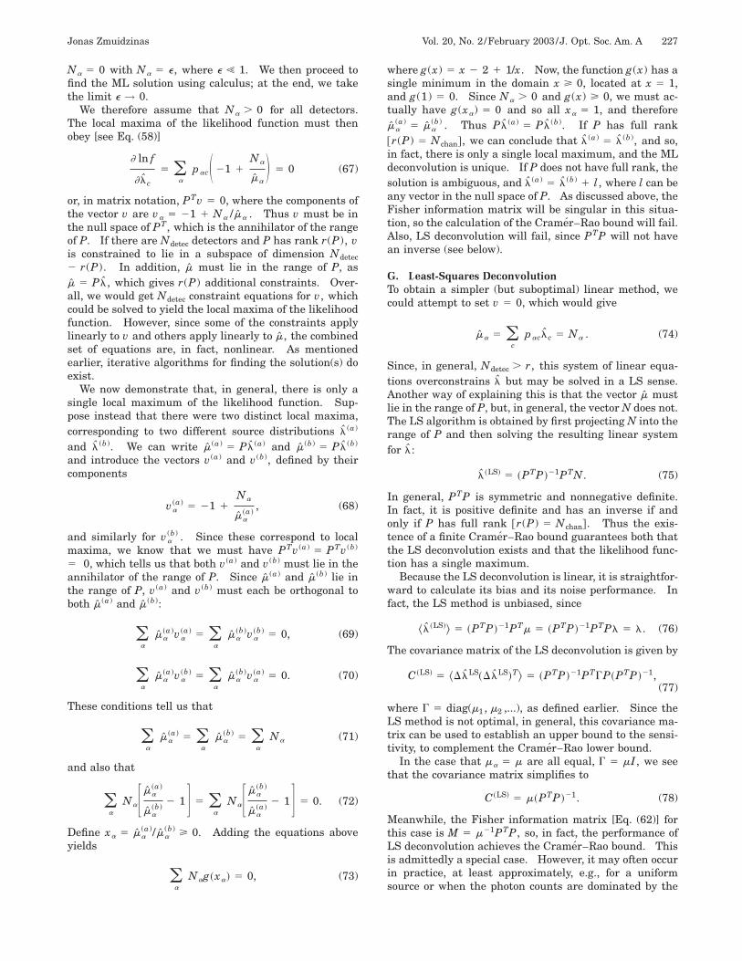
C. Pairwise CombinationWe compare two types of beam combination. The firstcase is the usual pairwise combination, in which we focuson measuring the fringe visibilities and fringe phases thatcan be obtained from the T(T 2 1)/2 telescope baselinepairs. To do this, the light from each telescope must firstbe split into T 2 1 beams. We assume that the fringemeasurement is done using four detectors per baseline, asshown in Fig. 1. The scattering matrix of the beam com-biner produces the following four linear combinations:

b1~t, t8! 51

2AT 2 1~bt 1 bt8!,

b2~t, t8! 51

2AT 2 1~bt 2 bt8!,

b3~t, t8! 51

2AT 2 1~bt 1 ibt8!,

b4~t, t8! 51

2AT 2 1~ibt 1 bt8!.

Here bt and bt8 represent the single-mode wave ampli-tudes corresponding to the light collected by telescopes tand t8, and the four amplitudes bk(t, t8) (here k5 1,..., 4) represent the four combinations of light fromthe two telescopes that are being detected to produce thecorresponding photon counts Nk(t, t8). To avoid repeat-ing telescope pairs, we require T > t . t8 > 1. The totalnumber of detectors in this scheme is 2T(T 2 1). Thedetector index a 5 1,..., 2T(T 2 1) uniquely specifies abaseline pair (t, t8) as well as one of the four beam-combiner outputs k; we can set a(t, t8, k) 5 @4(T 2 1)2 2t8)](t8 2 1) 1 4(t 2 2) 1 k. For example, Eq. (48)reads

Ra~V, n! 51

4~T 2 1 !uSt

~rec!~u! 1 iSt8~rec!

~u!u2 (83)

Fig. 1. Schematic diagram of the pairwise beam combinationscheme for a single baseline between telescopes t and t8. Theinputs t and t8 on the left represent the single-mode beams fromthe two telescopes, after division T 2 1 ways. The four outputson the right are sent to photon-counting detectors.

for the case that a 5 a(t, t8, k 5 3).It is straightforward to verify that the first two beam

combinations produce symmetric angular response func-tions, whereas the latter two produce antisymmetric re-sponse functions (apart from a constant offset term).Thus both types of beam combination are needed touniquely determine the image of a source. The latter twobeam combinations are readily produced with a 50%beam splitter; at microwave frequencies, the equivalentdevice is known as a 90° 3-dB hybrid. The first two com-binations can be obtained by use of the optical equivalentof a microwave 180° 3-dB hybrid; such devices are cur-rently being investigated for nulling interferometry.49,50

All four combinations can be gotten simultaneously byuse of a two-way power splitter (or a 50% beam splitter),as shown in Fig. 1. It is straightforward to verify that forthis beam combination scheme all the power (photons)collected by the telescopes is absorbed by the detectors.Equivalently, the scattering matrix of the beam combineris unitary and only couples input ports to output ports.

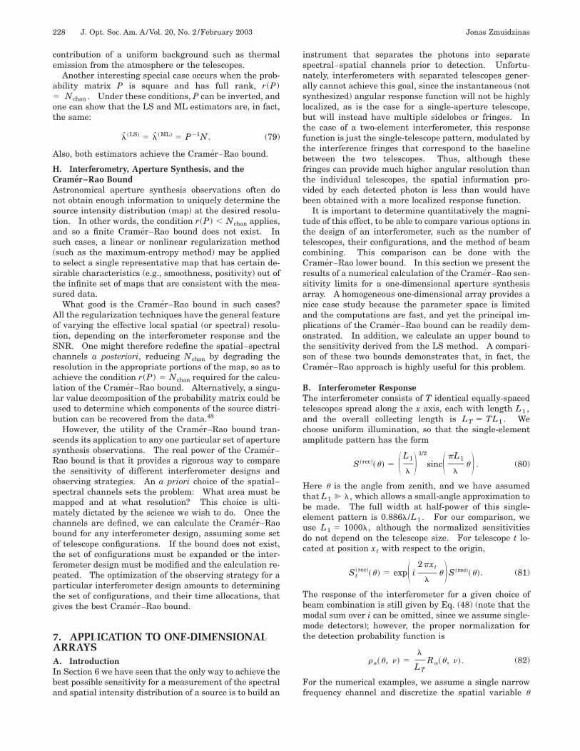
D. Butler CombinationAs shown in Fig. 2, the second type of beam combinationmethod we investigate is the standard Butler matrixbeam-forming network,51 which is used with microwavephased-array antennas to produce a set of localizedbeams, each pointing in a different direction. This ap-proach is analogous to the image-plane beam recombina-tion used in Fizeau interferometry. Although similarfree-space optical techniques could be used for microwavebeam forming, Butler beam formers use guided-wavecomponents (coaxial or waveguide) and are thereforemuch smaller physically.

The key idea behind the Butler matrix is to produce alinear-stepped phase gradient across the antenna or tele-scope array in order to steer the beam of the array.Mathematically, the T outputs ba , which are sent to thephoton-counting detectors, are given in terms of the Tsingle-mode inputs bt from the telescopes by

ba 51

AT(t51

T

bt expS i2pat

T D , (84)

which, in essence, is just a discrete Fourier transform.The Butler matrix is actually a hardware implementationof this concept that is analogous to the fast-Fourier-transform algorithm. Power conservation, or unitarity ofthe beam-combiner scattering matrix, follows from Parse-val’s theorem. The typical angular response functions forpairwise and Butler combining are compared in Fig. 3.

Fig. 2. Schematic diagram of the Butler matrix all-on-one beamcombination scheme. The inputs on the left represent thesingle-mode beams from all T telescopes; each of the T outputs onthe right, which are sent to photon-counting detectors, containsome contribution from all T telescope inputs.


E. Numerical CalculationsWe consider array configurations of three, six, and tenuniformly spaced telescopes, as shown in Table 1. Sincethe maximum baseline of all the array configurationsshown in Table 1 is Bmax 5 45L1 and the maximum base-line controls the spatial resolution, we use Nchan 5 41spatial pixels in the calculations.

As shown in Table 1, the calculation also includes Nspacdifferent telescope spacings, ranging from close-packed todilute arrays. The source is observed repeatedly withdifferent telescope spacings; this is an example of aper-ture synthesis in one dimension. For example, we as-sume that the three-telescope array observes the sourcein a total of Nspac 5 44 different configurations. The firstconfiguration corresponds to a close-packed array, inwhich the telescope spacing is S 5 L1 . The various con-figurations are obtained by incrementing the telescopespacing S by DS; thus the second configuration has S5 1.5L, the third has S 5 2.0L1 , and so on. The mostdilute configuration has S 5 22.5L1 . The correspondingpositions of the three telescopes are x1 5 2S, x2 5 0, andx3 5 S.

To account for these various configurations, we imaginethat there are actually Nspac Ndetec different virtual detec-tors, now indexed by b, where Ndetec is the physical num-ber of detectors (labeled by a) in any one configuration.Note that we must have Nchan , Nspac Ndetec ; otherwise,

Fig. 3. Comparison of the angular response functions for pair-wise and Butler beam combining. Top, typical response corre-sponding to two telescopes in a pair-combined array; the separa-tion between the telescopes is 27L1 for this example. Bottom,typical response of a Butler-combined array; in this case, thereare 10 uniformly spaced telescopes, with a distance 3L1 betweentelescopes, so that the array size is 27L1 .

Table 1. Array Configurationsa

Tb Nspacc Smin

d Smaxd DSd Bmax

e

3 44 1.0 22.5 0.5 45.06 17 1.0 9.0 0.5 45.0

10 9 1.0 5.0 0.5 45.0

a All dimensions are scaled to the telescope size L1 .b The number of telescopes.c The number of element spacings.d Minimum, maximum, and step size for the element spacings.e The maximum baseline.

the probability matrix P cannot have full rank, and theFisher information matrix [Eq. (59)] will be singular. Asdescribed in the discussion of aperture synthesis at theend of Section 5, the detection probabilities for any oneconfiguration are reduced by the factor (Nspac )21. Weare splitting up the total observing time into Nspac differ-ent sessions of equal duration, one per configuration; thetotal probability over the course of the entire integrationfor a photon to be detected by the array in some particularconfiguration is (Nspac )21. As a check, we verified thatin all cases the total combined probability for detectingphotons from the central spatial pixels c in any of the vir-tual detectors b was near unity: (b51

(Nspac Ndetec)pbc ' 1.We also consider two types of source: uniform sources

and point sources. For uniform sources, we set lc 5 1for all Nchan spatial pixels; for point sources, we set lc5 1 only for the central pixel and set all others to zero.

F. ResultsFigure 4 shows the results for a uniform source with But-ler beam combination. The vertical axis is the normal-ized Cramer–Rao sensitivity bound, calculated with inequality (60). This sensitivity would be unity for an idealinstrument, that is, a single telescope with an aperturelarge enough to resolve the spatial pixels but with thesame total effective collecting area as the interferometer(i.e., with a neutral-density filter or attenuator to reducethe total number of detected photons to match the inter-ferometer). A sensitivity above unity implies that theuse of an interferometer incurs a penalty owing to its in-ability to fully determine from which spatial pixel eachdetected photon came. As Fig. 4 shows, adding moretelescopes improves the sensitivity; the reason for this isthat the quality of the instantaneous beam pattern im-proves. For this particular example, the sensitivity pen-

Fig. 4. Variation of the normalized sensitivity with telescopearray size for the case of Butler beam combination. The sourceis assumed to have a uniform spatial distribution. The horizon-tal axis gives the spatial position u in units of l/L1 ; note thatthe full width at half-power of the single-element pattern is0.886l/L1 . The vertical axis gives the Cramer–Rao normalizedsensitivity bound (see text for details). For Butler beam combi-nation, increasing the array size improves the normalized sensi-tivity. The dotted curve shows that the sensitivity degradationtoward the edges of the field of view scales as the reciprocal of thesingle-element beam pattern. The upper sensitivity limit calcu-lated with the LS deconvolution method is indistinguishablefrom Cramer–Rao bound; thus this plot gives the actual achiev-able sensitivity.


alty for the Butler-combined interferometer is a factor of;3 for a ten-telescope array. The variation of the sensi-tivity across the field of view is seen to scale with the in-verse of the single-element power pattern, as shown bythe dotted curve in Fig. 4. The reason for this is that theCramer–Rao sensitivity bound includes the effects ofnoise cross talk between the spatial pixels that arise fromthe nonideal interferometer beam patterns. For this ex-ample, the upper limit to sensitivity derived from the LSdeconvolution method [by use of Eq. (77)] coincides withthe lower limit set by the Cramer–Rao bound; thus eithergives the true sensitivity.

Figure 5 shows the comparable uniform-source resultswith pairwise beam combination. In this case, the nor-malized sensitivity (which takes out the effect of the totalcollecting area) shows no improvement as the array size isincreased. This is because the quality of the instanta-neous beam patterns remains unchanged: The beampatterns are always those of two-element interferometers.Again, the sensitivity scales inversely with the single-element pattern; however, the sensitivity penalty relativeto an ideal instrument is now a factor of ;10. Again, theLS and Cramer–Rao bounds coincide, so either yields thetrue sensitivity. The comparison between the Butler-combined and the pairwise-combined ten-element arraysfor uniform sources is shown more directly in Fig. 6; the

Fig. 5. Similar to Fig. 4 but calculated for pairwise beam com-bination. Normalized sensitivity is essentially independent ofarray size. Again, the upper limit from the LS method is calcu-lated to be the same as the Cramer–Rao lower bound.

Fig. 6. Comparison of normalized sensitivities for Butler versuspairwise beam combining for a ten-element array when uniformsources are observed; the sensitivity advantage for Butler com-bining is more than a factor of 3.

Butler-combined array enjoys a sensitivity advantage inexcess of a factor of 3 for this example.

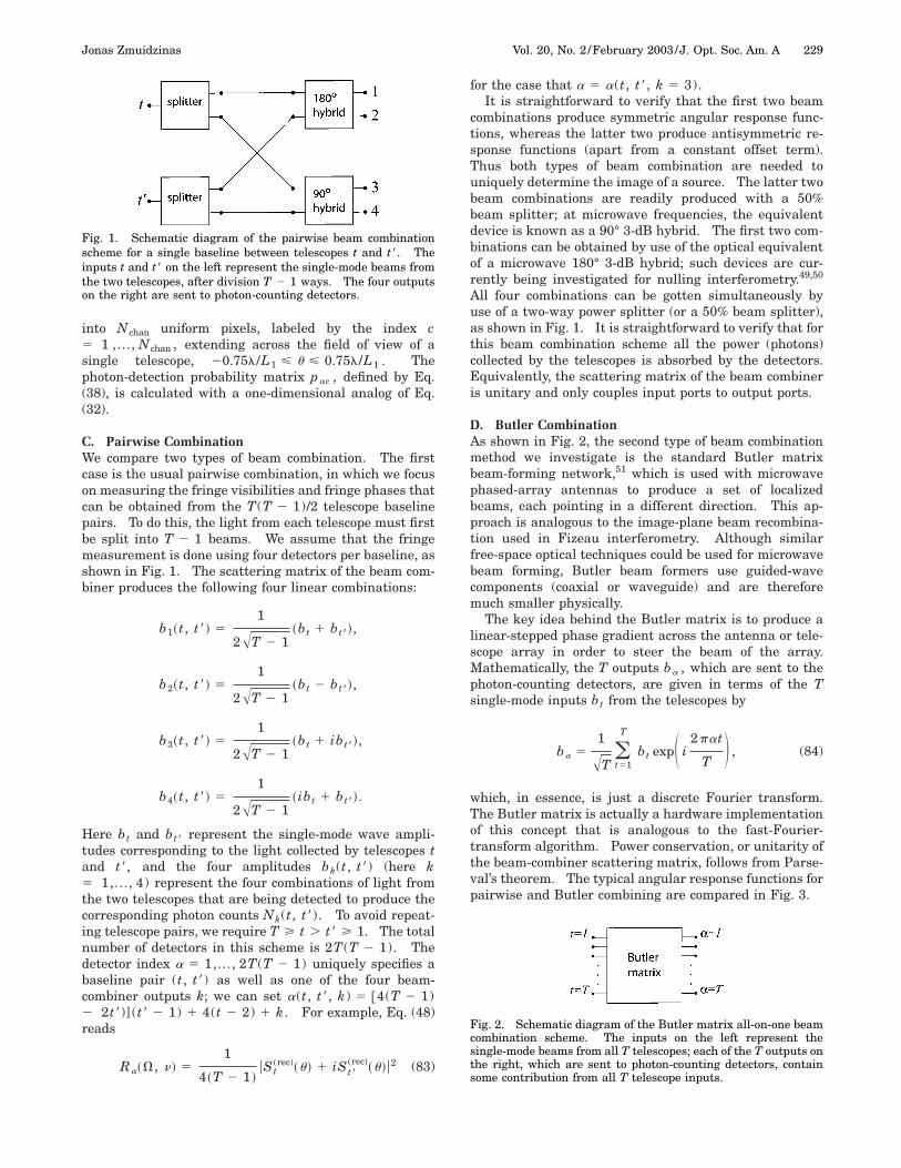
A similar comparison for the case of point sources isshown in Figs. 7–9. There now is a difference betweenthe LS upper bound and the Cramer–Rao lower bound forthe case of Butler combining (Fig. 7) but not for pairwisecombining (Fig. 8). However, we see that the LS upperbound still allows us to demonstrate the superiority of ar-rays with larger numbers of elements and of Butler com-bining over pairwise combining.

The normalized Cramer–Rao sensitivities for the pointsource itself are quite comparable in all cases, which weexpect, because we can, in essence, sum all the photonsdetected to estimate the brightness of the source. How-ever, the sensitivity for the off-source pixels tells a muchdifferent story. Here Butler combination enjoys a largesensitivity advantage, approximately an order of magni-tude for the ten-element array. Note that for the Butler-combined arrays, the sensitivity of the off-source pixels isactually substantially better than for the on-source pixels.This is highly desirable: It gives the array more sensi-tivity to see faint sources in the presence of a brighter

Fig. 7. Similar to Fig. 4 but calculated for a point source in thecenter of the field instead of for a uniform source. Note that al-though the normalized sensitivity to the point source is nearlyconstant, the sensitivity for off-source pixels improves substan-tially with array size. The upper limit from the LS method issomewhat worse than the Cramer–Rao lower bound and isshown as the upper solid curve for the ten-element array. Thiscurve lies near the Cramer–Rao lower bound for the six-elementarray and below the bound for the three-element array.

Fig. 8. Similar to Fig. 7 but with pairwise beam combination as-sumed; there is no sensitivity improvement with array size.The sensitivity of the LS method is indistinguishable from theCramer–Rao bound, so the plot gives the actual sensitivity.


nearby object. An ideal instrument, such as a largesingle-aperture telescope, would, in fact, have sc 5 0 forthe off-source pixels, since the detectors corresponding tothese pixels do not receive any photons. (Of course, thisis not entirely true for real telescope systems owing toscattered light.)

8. CONCLUDING REMARKSIn this paper we have made the case that the instanta-neous angular response functions of an interferometergovern its sensitivity: Interferometers with more com-pact and localized response functions are more sensitive.The physical reason for this is simple and clear: Such in-terferometers obtain more spatial information per photondetected. We have demonstrated this effect by numeri-cally calculating the Cramer–Rao sensitivity limits forthe simple case of homogeneous, equally spaced, one-dimensional aperture synthesis arrays that use eitherButler or pairwise beam combining. These calculationsshow that Butler beam combining, which is analogous tothe image-plane combination used in Fizeau interferom-etry, is substantially more sensitive, which we expect,since the response functions are more compact. In addi-tion, our example shows that when telescopes are addedto the array the sensitivity of a Butler-combined interfer-ometer improves much more rapidly than that of the totalcollecting area. However, it is important to rememberthat the imperfect beam patterns of sparse-aperture in-terferometers extract a sensitivity penalty as comparedwith filled-aperture telescopes, even after accounting forthe differences in collecting areas.

The Cramer–Rao bound appears to be a very interest-ing and useful tool for the study and optimization of in-terferometer designs. The approach presented in thispaper can readily be applied to two-dimensional arraysthat are of any configuration and that use any type ofbeam combination method. Our approach, which isbased on scattering matrices, is especially well suited todescribe beam combination by use of guided-wave (inte-

Fig. 9. Comparison of normalized point-source sensitivities forButler combination and pairwise combination for a ten-elementarray. Although the sensitivities to the point source itself arecomparable, Butler combination is an order of magnitude moresensitive for off-source pixels. The upper solid curve gives theLS upper sensitivity limit for the Butler-combined array, and itlies well below the Cramer–Rao lower bound for the pairwise-combined array.

grated) optics. Although we have discussed only homo-geneous arrays, in which all telescopes are identical, theformalism can readily be adapted to handle heteroge-neous arrays. The Cramer–Rao sensitivity bounds wereobtained for very idealized circumstances, in which wehave included only the counting statistics of the photonsarriving from the source. However, it is again not diffi-cult to extend our results to include effects such as back-ground noise, which is due to thermal emission from thetelescope or atmosphere and from detector dark currentor read noise or both. Although these effects are impor-tant in real applications and should be included in morerealistic calculations, we have ignored them to limit theparameter space and to focus on the fundamental issuesinvolved. In closing, we encourage other researcherswho are involved in interferometer design to investigatethe applicability of the Cramer–Rao approach for deter-mining the sensitivity trade-offs for real arrays and for arange of astrophysical problems. As an example, itwould be interesting to study the exoplanet detectionproblem, under realistic constraints such as a fixed totalcollecting area.

ACKNOWLEDGMENTSThe author thanks W. C. Danchi, S. H. Moseley, T. G.Phillips, S. Padin, and J. R. P. Angel for useful discus-sions. He is particularly indebted to one of the referees,whose diligent and thorough reading of the manuscript,detailed suggestions, and numerous comments led to sub-stantial revision and improvement of the paper. The au-thor is grateful for the generous support of Alex Lidow,Caltech Trustee.

The author can be reached by e-mail at [email protected].

REFERENCES1. A. Quirrenbach, ‘‘Optical interferometry,’’ Annu. Rev. As-

tron. Astrophys. 39, 353–401 (2001).2. S. K. Saha, ‘‘Modern optical astronomy: technology and

impact of interferometry,’’ Rev. Mod. Phys. 74, 551–600(2002).

3. See http://olbin.jpl.nasa.gov.4. See http://www.nrao.edu.5. M. Shao, ‘‘SIM: the space interferometry mission,’’ in

Astronomical Interferometry, R. D. Reasenberg, ed., Proc.SPIE 3350, 536–540 (1998), see also http://sim.jpl.nasa.gov.

6. C. A. Beichman, ‘‘Terrestrial Planet Finder: the searchfor life-bearing planets around other stars,’’ in AstronomicalInterferometry, R. D. Reasenberg, ed., Proc. SPIE 3350,719–723 (1998), see also http://planetquest.jpl.nasa.gov.

7. A. J. Penny, A. Leger, J. Mariotti, C. Schalinski, C. Eiroa, R.J. Laurance, and M. Fridlund, ‘‘Darwin interferometer,’’ inAstronomical Interferometry, R. D. Reasenberg, ed., Proc.SPIE 3350, 666–671 (1998), see also http://sci.esa.int/darwin.

8. D. Leisawitz, J. C. Mather, S. Harvey Moseley, and X.Zhang, ‘‘The Submillimeter Probe of the Evolution of Cos-mic Structure (SPECS),’’ Astrophys. Space Sci. 269, 563–567 (1999).

9. M. Shao, W. Danchi, M. J. DiPirro, M. Dragovan, L. D.Feinberg, M. Hagopian, W. D. Langer, C. R. Lawrence, P. R.Lawson, D. T. Leisawitz, J. C. Mather, S. H. Moseley, M. R.Swain, H. W. Yorke, and X. Zhang, ‘‘Space-based interfero-

https://www.researchgate.net/publication/258911384_SIM_the_space_interferometry_mission?el=1_x_8&enrichId=rgreq-3ed5109066be9fc8224330b6319b1be5-XXX&enrichSource=Y292ZXJQYWdlOzEwOTE1NjIyO0FTOjEwMjM3ODMwMDc3MjM1OUAxNDAxNDIwMjk3MjMw




https://www.researchgate.net/publication/2235935_Modern_optical_astronomy_Technology_and_impact_of_interferometry?el=1_x_8&enrichId=rgreq-3ed5109066be9fc8224330b6319b1be5-XXX&enrichSource=Y292ZXJQYWdlOzEwOTE1NjIyO0FTOjEwMjM3ODMwMDc3MjM1OUAxNDAxNDIwMjk3MjMw




https://www.researchgate.net/publication/234519972_Terrestrial_Planet_Finder_the_search_for_life-bearing_planets_around_other_stars?el=1_x_8&enrichId=rgreq-3ed5109066be9fc8224330b6319b1be5-XXX&enrichSource=Y292ZXJQYWdlOzEwOTE1NjIyO0FTOjEwMjM3ODMwMDc3MjM1OUAxNDAxNDIwMjk3MjMw





https://www.researchgate.net/publication/228870755_Optical_Interferometry?el=1_x_8&enrichId=rgreq-3ed5109066be9fc8224330b6319b1be5-XXX&enrichSource=Y292ZXJQYWdlOzEwOTE1NjIyO0FTOjEwMjM3ODMwMDc3MjM1OUAxNDAxNDIwMjk3MjMw

https://www.researchgate.net/publication/228870755_Optical_Interferometry?el=1_x_8&enrichId=rgreq-3ed5109066be9fc8224330b6319b1be5-XXX&enrichSource=Y292ZXJQYWdlOzEwOTE1NjIyO0FTOjEwMjM3ODMwMDc3MjM1OUAxNDAxNDIwMjk3MjMw

https://www.researchgate.net/publication/227010283_The_Submillimeter_Probe_of_the_Evolution_of_Cosmic_Structure_SPECS?el=1_x_8&enrichId=rgreq-3ed5109066be9fc8224330b6319b1be5-XXX&enrichSource=Y292ZXJQYWdlOzEwOTE1NjIyO0FTOjEwMjM3ODMwMDc3MjM1OUAxNDAxNDIwMjk3MjMw





metric telescopes for the far infrared,’’ in Interferometry inOptical Astronomy, P. J. Lena and A. Quirrenbach, eds.,Proc. SPIE 4006, 772–781 (2000).

10. D. T. Leisawitz, W. C. Danchi, M. J. DiPirro, L. D. Feinberg,D. Y. Gezari, M. Hagopian, W. D. Langer, J. C. Mather, S. H.Moseley, M. Shao, R. F. Silverberg, J. Staguhn, M. R.Swain, H. W. Yorke, and X. Zhang, ‘‘Scientific motivationand technology requirements for the SPIRIT and SPECSfar-infrared/submillimeter space interferometers,’’ in UV,Optical, and IR Space Telescopes and Instruments, J. B.Breckinridge and P. Jakobsen, eds., Proc. SPIE 4013, 36–46(2000).

11. A. Blain, R. Ivison, and I. Smail, ‘‘Observational limits tosource confusion in the millimetre/submillimetre wave-band,’’ Mon. Not. R. Astron. Soc. 296, L29–L33 (1998).

12. I. Smail, R. J. Ivison, and A. W. Blain, ‘‘A deep submillime-ter survey of lensing clusters: a new window on galaxyformation and evolution,’’ Astrophys. J. 490, L5–L8 (1997).

13. D. Hughes, S. Serjeant, J. Dunlop, M. Rowan-Robinson, A.Blain, R. G. Mann, R. Ivison, J. Peacock, A. Efstathiou, W.Gear, S. Oliver, A. Lawrence, M. Longair, P. Goldschmidt,and T. Jenness, ‘‘High-redshift star formation in the HubbleDeep Field revealed by a submillimetre-wavelength sur-vey,’’ Nature 394, 241–247 (1998).

14. A. Barger, L. Cowie, D. Sanders, E. Fulton, Y. Taniguchi, Y.Sato, K. Kawara, and H. Okuda, ‘‘Submillimetre-wavelength detection of dusty star-forming galaxies at highredshift,’’ Nature 394, 248–251 (1998).

15. F. Roddier, ‘‘Pupil plane versus image plane in Michelsonstellar interferometry,’’ J. Opt. Soc. Am. A 3, 2160–2166(1986).

16. W. Traub, ‘‘Combining beams from separated telescopes,’’Appl. Opt. 25, 528–532 (1986).

17. S. Prasad and S. R. Kulkarni, ‘‘Noise in optical synthesisimages. I. Ideal Michelson interferometer,’’ J. Opt. Soc.Am. A 6, 1702–1714 (1989).

18. M. Faucherre, B. Delabre, P. Dierickx, and F. Merkle,‘‘Michelson versus Fizeau type beam combination—Is therea difference?’’ in Amplitude and Intensity Spatial Interfer-ometry, Proc. SPIE 1237, 206–217 (1990).

19. S. R. Kulkarni, S. Prasad, and T. Nakajima, ‘‘Noise in opti-cal synthesis images. II. Sensitivity of an nC2 interfer-ometer with bispectrum imaging,’’ J. Opt. Soc. Am. A 8,499–510 (1991).

20. S. Prasad, ‘‘Sensitivity limits on an image-plane fiber inter-ferometer at low-light levels,’’ in Amplitude and IntensitySpatial Interferometry II, J. B. Breckinridge, ed., Proc.SPIE 2200, 51–59 (1994).

21. L. Mugnier, G. Rousset, and F. Cassaing, ‘‘Aperture configu-ration optimality criterion for phased arrays of optical tele-scopes,’’ J. Opt. Soc. Am. A 13, 2367–2374 (1996).

22. F. Roddier and S. T. Ridgway, ‘‘Filling factor and signal-to-noise ratios in optical interferometric arrays,’’ Publ. Astron.Soc. Pac. 111, 990–996 (1999).

23. T. Nakajima, ‘‘Sensitivity of a ground-based infrared inter-ferometer for aperture synthesis imaging,’’ Publ. Astron.Soc. Pac. 113, 1289–1299 (2001).

24. T. Nakajima and H. Matsuhara, ‘‘Sensitivity of an imagingspace infrared interferometer,’’ Appl. Opt. 40, 514–526(2001).

25. The author is preparing a manuscript to be called ‘‘Thermalnoise and correlations in photon detection.’’

26. S. W. Wedge, ‘‘Computer-aided design of noise microwavecircuits,’’ Ph.D. thesis (California Institute of Technology,Pasadena, Calif., 1991).

27. S. W. Wedge and D. B. Rutledge, ‘‘Wave computations formicrowave education,’’ IEEE Trans. Educ. 36, 127–131(1993).

28. H. Bosma, ‘‘On the theory of linear noisy systems,’’ PhilipsRes. Rep. Suppl. 10, 1–190 (1967).

29. S. W. Wedge and D. B. Rutledge, ‘‘Noise waves and passivelinear multiports,’’ IEEE Microwave Guid. Wave Lett. 1,117–119 (1991).

30. S. W. Wedge and D. B. Rutledge, ‘‘Wave techniques for noise

modeling and measurement,’’ IEEE Trans. MicrowaveTheory Tech. 40, 2004–2012 (1992).

31. in Principles of Microwave Circuits, Vol. 8 of M.I.T. Radia-tion Laboratory Series, C. G. Montgomery, R. H. Dicke, andE. M. Purcell, eds. (McGraw-Hill, New York, 1948), Chap. 9,pp. 317–333.

32. W. K. Kahn and W. Wasylkiwskyj, ‘‘Coupling, radiation, andscattering by antennas,’’ in Proceedings of the Symposiumon Generalized Networks, Vol. 16 of Microwave Research In-stitute Symposia Series (Polytechnic, New York, 1966), pp.83–114.

33. A. C. Gately and D. J. R. Stock, and B. R.-S. Cheo, ‘‘A net-work description for antenna problems,’’ Proc. IEEE 56,1181–1193 (1968).

34. S. Withington and J. Murphy, ‘‘Modal analysis of partiallycoherent submillimeter-wave quasi-optical systems,’’ IEEETrans. Antennas Propag. 46, 1651–1659 (1998).

35. P. Kern and F. Malbet, eds., Integrated Optics for Astro-nomical Interferometry (Bastinelli-Guirimand, Grenoble,France, 1996).

36. J. Berger, P. Haguenauer, P. Kern, K. Perraut, F. Malbet, I.Schanen, M. Severi, R. Millan-Gabet, and W. Traub, ‘‘Inte-grated optics for astronomical interferometry. IV. Firstmeasurements of stars,’’ Astron. Astrophys. 376, L31–L34(2001).

37. L. A. Shepp and Y. Vardi, ‘‘Maximum likelihood reconstruc-tion for emission tomography,’’ IEEE Trans. Med. Imaging1, 113–122 (1982).

38. R. Molina, J. Nunez, F. J. Cortijo, and J. Mateos, ‘‘Imagerestoration in astronomy—a Bayesian perspective,’’ IEEESignal Process. Mag. 18, 11–29 (2001).

39. A. J. Weiss and E. Weinstein, ‘‘Fundamental limitations inpassive time-delay estimation—Part I: narrow-bandsystems,’’ IEEE Trans. Acoust., Speech, Signal Process.ASSP-32, 472–486 (1983).

40. E. Weinstein and A. J. Weiss, ‘‘Fundamental limitations inpassive time-delay estimation—Part II: wide-band sys-tems,’’ IEEE Trans. Acoust., Speech, Signal Process. ASSP-32, 1064–1078 (1984).

41. K. L. Bell, Y. Ephraim, and H. L. Van Trees, ‘‘Explicit Ziv–Zakai lower bound for bearing estimation,’’ IEEE Trans.Signal Process. 44, 2810–2824 (1996).

42. J. G. Cohen, ‘‘Tests of the photometric accuracy of imagerestoration using the maximum entropy algorithm,’’ Astron.J. 101, 734–737 (1991).

43. P. Jakobsen, P. Greenfield, and R. Jedrzejcwski, ‘‘TheCramer–Rao lower bound and stellar photometry with ab-errated HST images,’’ Astron. Astrophys. 253, 329–332(1992).

44. C. H. Hua, N. H. Clinthorne, S. J. Wilderman, J. W.LeBlanc, and W. L. Rogers, ‘‘Quantitative evaluation of in-formation loss for Compton cameras,’’ IEEE Trans. Nucl.Sci. 46, 587–593 (1999).

45. H. Cramer, Mathematical Methods of Statistics (PrincetonU. Press, Princeton, N. J., 1946).

46. C. R. Rao, ‘‘Information and accuracy attainable in the es-timation of statistical parameters,’’ Bull. Calcutta Math.Soc. 37, 81–91 (1945).

47. H. L. Van Trees, Detection, Estimation, and ModulationTheory, Part I (Wiley, New York, 1968).

48. P. Stoica and T. L. Marzetta, ‘‘Parameter estimation prob-lems with singular information matrices,’’ IEEE Trans. Sig-nal Process. 49, 87–90 (2001).

49. E. Serabyn, ‘‘Nulling interferometry and planet detection,’’in Principles of Long Baseline Stellar Interferometry,Course Notes from the 1999 Michelson Summer School, Au-gust 15–19, 1999, P. R. Lawson, ed., NASA/JPL Publication00-009 Rev. 1 03-01 (NASA/Jet Propulsion Laboratory,Pasadena, Calif. 2000), pp. 275–292.

50. E. Serabyn and M. M. Colavita, ‘‘Fully symmetric nullingbeam combiners,’’ Appl. Opt. 40, 1668–1671 (2001).

51. J. Butler and R. Lowe, ‘‘Beam-forming matrix simplifies de-sign of electronically scanned antennas,’’ Electron. Des. 9,170–173 (1961).

https://www.researchgate.net/publication/1816771_Observational_Limits_to_Source_Confusion_in_the_Millimetresubmillimetre?el=1_x_8&enrichId=rgreq-3ed5109066be9fc8224330b6319b1be5-XXX&enrichSource=Y292ZXJQYWdlOzEwOTE1NjIyO0FTOjEwMjM3ODMwMDc3MjM1OUAxNDAxNDIwMjk3MjMw



https://www.researchgate.net/publication/228790913_High-redshift_star_formation_in_the_Hubble_Deep_Field_revealed_by_a_submillimetre-wavelength_survey?el=1_x_8&enrichId=rgreq-3ed5109066be9fc8224330b6319b1be5-XXX&enrichSource=Y292ZXJQYWdlOzEwOTE1NjIyO0FTOjEwMjM3ODMwMDc3MjM1OUAxNDAxNDIwMjk3MjMw






https://www.researchgate.net/publication/239007632_Noise_in_optical_synthesis_Images_Pt_1_Ideal_Michelson_interferometer?el=1_x_8&enrichId=rgreq-3ed5109066be9fc8224330b6319b1be5-XXX&enrichSource=Y292ZXJQYWdlOzEwOTE1NjIyO0FTOjEwMjM3ODMwMDc3MjM1OUAxNDAxNDIwMjk3MjMw



https://www.researchgate.net/publication/255538593_Noise_in_optical_synthesis_images_II_Sensitivity_of_ann_C_2_interferometer_with_bispectrum_imaging?el=1_x_8&enrichId=rgreq-3ed5109066be9fc8224330b6319b1be5-XXX&enrichSource=Y292ZXJQYWdlOzEwOTE1NjIyO0FTOjEwMjM3ODMwMDc3MjM1OUAxNDAxNDIwMjk3MjMw




https://www.researchgate.net/publication/239007765_Aperture_configuration_optimality_criterion_for_phased_arrays_of_optical_telescopes?el=1_x_8&enrichId=rgreq-3ed5109066be9fc8224330b6319b1be5-XXX&enrichSource=Y292ZXJQYWdlOzEwOTE1NjIyO0FTOjEwMjM3ODMwMDc3MjM1OUAxNDAxNDIwMjk3MjMw



https://www.researchgate.net/publication/249142679_Filling_Factor_and_Signal-to-Noise_Ratios_in_Optical_Interferometric_Arrays?el=1_x_8&enrichId=rgreq-3ed5109066be9fc8224330b6319b1be5-XXX&enrichSource=Y292ZXJQYWdlOzEwOTE1NjIyO0FTOjEwMjM3ODMwMDc3MjM1OUAxNDAxNDIwMjk3MjMw



https://www.researchgate.net/publication/2231326_Sensitivity_of_a_Ground-Based_Infrared_Interferometer_for_Aperture_Synthesis_Imaging?el=1_x_8&enrichId=rgreq-3ed5109066be9fc8224330b6319b1be5-XXX&enrichSource=Y292ZXJQYWdlOzEwOTE1NjIyO0FTOjEwMjM3ODMwMDc3MjM1OUAxNDAxNDIwMjk3MjMw



https://www.researchgate.net/publication/254753934_On_the_Theory_of_Linear_Noise_Systems?el=1_x_8&enrichId=rgreq-3ed5109066be9fc8224330b6319b1be5-XXX&enrichSource=Y292ZXJQYWdlOzEwOTE1NjIyO0FTOjEwMjM3ODMwMDc3MjM1OUAxNDAxNDIwMjk3MjMw

https://www.researchgate.net/publication/254753934_On_the_Theory_of_Linear_Noise_Systems?el=1_x_8&enrichId=rgreq-3ed5109066be9fc8224330b6319b1be5-XXX&enrichSource=Y292ZXJQYWdlOzEwOTE1NjIyO0FTOjEwMjM3ODMwMDc3MjM1OUAxNDAxNDIwMjk3MjMw

https://www.researchgate.net/publication/3118186_Wave_Techniques_for_Noise_Modeling_and_Measurement?el=1_x_8&enrichId=rgreq-3ed5109066be9fc8224330b6319b1be5-XXX&enrichSource=Y292ZXJQYWdlOzEwOTE1NjIyO0FTOjEwMjM3ODMwMDc3MjM1OUAxNDAxNDIwMjk3MjMw



https://www.researchgate.net/publication/5614274_Maximum_Likelihood_Reconstruction_for_Emission_Tomography?el=1_x_8&enrichId=rgreq-3ed5109066be9fc8224330b6319b1be5-XXX&enrichSource=Y292ZXJQYWdlOzEwOTE1NjIyO0FTOjEwMjM3ODMwMDc3MjM1OUAxNDAxNDIwMjk3MjMw



https://www.researchgate.net/publication/3136523_Quantitative_evaluation_of_information_loss_for_Compton_cameras?el=1_x_8&enrichId=rgreq-3ed5109066be9fc8224330b6319b1be5-XXX&enrichSource=Y292ZXJQYWdlOzEwOTE1NjIyO0FTOjEwMjM3ODMwMDc3MjM1OUAxNDAxNDIwMjk3MjMw




https://www.researchgate.net/publication/287663443_Beam_forming_matrix_simplifies_design_of_electronically_scanned_antenna?el=1_x_8&enrichId=rgreq-3ed5109066be9fc8224330b6319b1be5-XXX&enrichSource=Y292ZXJQYWdlOzEwOTE1NjIyO0FTOjEwMjM3ODMwMDc3MjM1OUAxNDAxNDIwMjk3MjMw



https://www.researchgate.net/publication/248850624_Integrated_optics_for_astronomical_interferometry_IV_First_measurements_of_stars?el=1_x_8&enrichId=rgreq-3ed5109066be9fc8224330b6319b1be5-XXX&enrichSource=Y292ZXJQYWdlOzEwOTE1NjIyO0FTOjEwMjM3ODMwMDc3MjM1OUAxNDAxNDIwMjk3MjMw





https://www.researchgate.net/publication/2990959_A_Network_Description_for_Antenna_Problems?el=1_x_8&enrichId=rgreq-3ed5109066be9fc8224330b6319b1be5-XXX&enrichSource=Y292ZXJQYWdlOzEwOTE1NjIyO0FTOjEwMjM3ODMwMDc3MjM1OUAxNDAxNDIwMjk3MjMw



https://www.researchgate.net/publication/3177627_Fundamental_limitations_in_passive_time-delay_estimation--Part_II_Wide-band_systems?el=1_x_8&enrichId=rgreq-3ed5109066be9fc8224330b6319b1be5-XXX&enrichSource=Y292ZXJQYWdlOzEwOTE1NjIyO0FTOjEwMjM3ODMwMDc3MjM1OUAxNDAxNDIwMjk3MjMw





https://www.researchgate.net/publication/241511083_Sensitivity_limits_on_an_image-plane_fiber_interferometer_at_low-light_levels?el=1_x_8&enrichId=rgreq-3ed5109066be9fc8224330b6319b1be5-XXX&enrichSource=Y292ZXJQYWdlOzEwOTE1NjIyO0FTOjEwMjM3ODMwMDc3MjM1OUAxNDAxNDIwMjk3MjMw




https://www.researchgate.net/publication/230710769_Scientific_motivation_and_technology_requirements_for_the_SPIRIT_and_SPECS_far-infraredsubmillimeter_space_interferometers?el=1_x_8&enrichId=rgreq-3ed5109066be9fc8224330b6319b1be5-XXX&enrichSource=Y292ZXJQYWdlOzEwOTE1NjIyO0FTOjEwMjM3ODMwMDc3MjM1OUAxNDAxNDIwMjk3MjMw









https://www.researchgate.net/publication/3177297_Fundamental_limitations_in_passive_time_delay_estimation--Part_I_Narrow-band_systems?el=1_x_8&enrichId=rgreq-3ed5109066be9fc8224330b6319b1be5-XXX&enrichSource=Y292ZXJQYWdlOzEwOTE1NjIyO0FTOjEwMjM3ODMwMDc3MjM1OUAxNDAxNDIwMjk3MjMw




https://www.researchgate.net/publication/3050126_Wave_Computations_for_Microwave_Education?el=1_x_8&enrichId=rgreq-3ed5109066be9fc8224330b6319b1be5-XXX&enrichSource=Y292ZXJQYWdlOzEwOTE1NjIyO0FTOjEwMjM3ODMwMDc3MjM1OUAxNDAxNDIwMjk3MjMw



https://www.researchgate.net/publication/3306262_Noise_Waves_and_Passive_Linear_Multiports?el=1_x_8&enrichId=rgreq-3ed5109066be9fc8224330b6319b1be5-XXX&enrichSource=Y292ZXJQYWdlOzEwOTE1NjIyO0FTOjEwMjM3ODMwMDc3MjM1OUAxNDAxNDIwMjk3MjMw



https://www.researchgate.net/publication/5621108_Combining_beams_from_separated_telescopes?el=1_x_8&enrichId=rgreq-3ed5109066be9fc8224330b6319b1be5-XXX&enrichSource=Y292ZXJQYWdlOzEwOTE1NjIyO0FTOjEwMjM3ODMwMDc3MjM1OUAxNDAxNDIwMjk3MjMw

https://www.researchgate.net/publication/5621108_Combining_beams_from_separated_telescopes?el=1_x_8&enrichId=rgreq-3ed5109066be9fc8224330b6319b1be5-XXX&enrichSource=Y292ZXJQYWdlOzEwOTE1NjIyO0FTOjEwMjM3ODMwMDc3MjM1OUAxNDAxNDIwMjk3MjMw

https://www.researchgate.net/publication/271541505_Michelson-_versus_Fizeau-type_beam_combination_is_there_a_difference?el=1_x_8&enrichId=rgreq-3ed5109066be9fc8224330b6319b1be5-XXX&enrichSource=Y292ZXJQYWdlOzEwOTE1NjIyO0FTOjEwMjM3ODMwMDc3MjM1OUAxNDAxNDIwMjk3MjMw




https://www.researchgate.net/publication/3010553_Modal_analysis_of_partially_coherent_submillimeter-wave_quasi-optical_systems?el=1_x_8&enrichId=rgreq-3ed5109066be9fc8224330b6319b1be5-XXX&enrichSource=Y292ZXJQYWdlOzEwOTE1NjIyO0FTOjEwMjM3ODMwMDc3MjM1OUAxNDAxNDIwMjk3MjMw



https://www.researchgate.net/publication/232777636_Submillimetre-wavelength_detection_of_dusty_star-forming_galaxies_at_high_redshift?el=1_x_8&enrichId=rgreq-3ed5109066be9fc8224330b6319b1be5-XXX&enrichSource=Y292ZXJQYWdlOzEwOTE1NjIyO0FTOjEwMjM3ODMwMDc3MjM1OUAxNDAxNDIwMjk3MjMw




https://www.researchgate.net/publication/247159648_Pupil_plane_versus_image_plane_in_Michelson_stellar_interferometry?el=1_x_8&enrichId=rgreq-3ed5109066be9fc8224330b6319b1be5-XXX&enrichSource=Y292ZXJQYWdlOzEwOTE1NjIyO0FTOjEwMjM3ODMwMDc3MjM1OUAxNDAxNDIwMjk3MjMw



https://www.researchgate.net/publication/5495635_Fully_Symmetric_Nulling_Beam_Combiners?el=1_x_8&enrichId=rgreq-3ed5109066be9fc8224330b6319b1be5-XXX&enrichSource=Y292ZXJQYWdlOzEwOTE1NjIyO0FTOjEwMjM3ODMwMDc3MjM1OUAxNDAxNDIwMjk3MjMw

https://www.researchgate.net/publication/5495635_Fully_Symmetric_Nulling_Beam_Combiners?el=1_x_8&enrichId=rgreq-3ed5109066be9fc8224330b6319b1be5-XXX&enrichSource=Y292ZXJQYWdlOzEwOTE1NjIyO0FTOjEwMjM3ODMwMDc3MjM1OUAxNDAxNDIwMjk3MjMw

https://www.researchgate.net/publication/5495487_Sensitivity_of_an_Imaging_Space_Infrared_Interferometer?el=1_x_8&enrichId=rgreq-3ed5109066be9fc8224330b6319b1be5-XXX&enrichSource=Y292ZXJQYWdlOzEwOTE1NjIyO0FTOjEwMjM3ODMwMDc3MjM1OUAxNDAxNDIwMjk3MjMw



https://www.researchgate.net/publication/243720892_Information_and_the_Accuracy_Attainable_in_the_Estimation_of_Statistical_Parameters?el=1_x_8&enrichId=rgreq-3ed5109066be9fc8224330b6319b1be5-XXX&enrichSource=Y292ZXJQYWdlOzEwOTE1NjIyO0FTOjEwMjM3ODMwMDc3MjM1OUAxNDAxNDIwMjk3MjMw



https://www.researchgate.net/publication/234226787_Tests_of_the_photometric_accuracy_of_image_restoration_using_the_maximum_entropy_algorithm?el=1_x_8&enrichId=rgreq-3ed5109066be9fc8224330b6319b1be5-XXX&enrichSource=Y292ZXJQYWdlOzEwOTE1NjIyO0FTOjEwMjM3ODMwMDc3MjM1OUAxNDAxNDIwMjk3MjMw



https://www.researchgate.net/publication/3317890_Parameter_estimation_problems_with_singular_information_matrices_IEEE_Trans_Signal_Proc_49_87-90?el=1_x_8&enrichId=rgreq-3ed5109066be9fc8224330b6319b1be5-XXX&enrichSource=Y292ZXJQYWdlOzEwOTE1NjIyO0FTOjEwMjM3ODMwMDc3MjM1OUAxNDAxNDIwMjk3MjMw



https://www.researchgate.net/publication/41481484_Computer-aided_design_of_low_noise_microwave_circuits?el=1_x_8&enrichId=rgreq-3ed5109066be9fc8224330b6319b1be5-XXX&enrichSource=Y292ZXJQYWdlOzEwOTE1NjIyO0FTOjEwMjM3ODMwMDc3MjM1OUAxNDAxNDIwMjk3MjMw



https://www.researchgate.net/publication/234327459_The_Cramer-Rao_lower_bound_and_stellar_photometry_with_aberrated_HST_images?el=1_x_8&enrichId=rgreq-3ed5109066be9fc8224330b6319b1be5-XXX&enrichSource=Y292ZXJQYWdlOzEwOTE1NjIyO0FTOjEwMjM3ODMwMDc3MjM1OUAxNDAxNDIwMjk3MjMw




https://www.researchgate.net/publication/3644839_Explicit_Ziv-Zakai_lower_bound_for_bearing_estimation?el=1_x_8&enrichId=rgreq-3ed5109066be9fc8224330b6319b1be5-XXX&enrichSource=Y292ZXJQYWdlOzEwOTE1NjIyO0FTOjEwMjM3ODMwMDc3MjM1OUAxNDAxNDIwMjk3MjMw



Cramer-Rao Sensitivity Limits for Astronomical Interferometry

Documents

Transcript of Cramer-Rao Sensitivity Limits for Astronomical Interferometry