
Seismic body-wave interferometry using noise ...
171
Purdue University Purdue e-Pubs Open Access eses eses and Dissertations 8-2016 Seismic body-wave interferometry using noise autocorrelations for crustal structure and a tutorial on 3D seismic processing and imaging using Madagascar Can Oren Purdue University Follow this and additional works at: hps://docs.lib.purdue.edu/open_access_theses Part of the Geophysics and Seismology Commons is document has been made available through Purdue e-Pubs, a service of the Purdue University Libraries. Please contact [email protected] for additional information. Recommended Citation Oren, Can, "Seismic body-wave interferometry using noise autocorrelations for crustal structure and a tutorial on 3D seismic processing and imaging using Madagascar" (2016). Open Access eses. 980. hps://docs.lib.purdue.edu/open_access_theses/980
-
Upload
khangminh22 -
Category
Documents
-
view
1 -
download
0
Transcript of Seismic body-wave interferometry using noise ...

Purdue UniversityPurdue e-Pubs
Open Access Theses Theses and Dissertations
8-2016
Seismic body-wave interferometry using noiseautocorrelations for crustal structure and a tutorialon 3D seismic processing and imaging usingMadagascarCan OrenPurdue University
Follow this and additional works at: https://docs.lib.purdue.edu/open_access_theses
Part of the Geophysics and Seismology Commons
This document has been made available through Purdue e-Pubs, a service of the Purdue University Libraries. Please contact [email protected] foradditional information.
Recommended CitationOren, Can, "Seismic body-wave interferometry using noise autocorrelations for crustal structure and a tutorial on 3D seismicprocessing and imaging using Madagascar" (2016). Open Access Theses. 980.https://docs.lib.purdue.edu/open_access_theses/980

Graduate School Form30 Updated ����������
PURDUE UNIVERSITYGRADUATE SCHOOL
Thesis/Dissertation Acceptance
This is to certify that the thesis/dissertation prepared
By
Entitled
For the degree of
Is approved by the final examining committee:
To the best of my knowledge and as understood by the student in the Thesis/Dissertation Agreement, Publication Delay, and Certification Disclaimer (Graduate School Form 32), this thesis/dissertation adheres to the provisions of Purdue University’s “Policy of Integrity in Research” and the use of copyright material.
Approved by Major Professor(s):
Approved by:Head of the Departmental Graduate Program Date
Can Oren
SEISMIC BODY-WAVE INTERFEROMETRY USING NOISE AUTO-CORRELATIONS FOR CRUSTAL STRUCTUREAND A TUTORIAL ON 3D SEISMIC PROCESSING AND IMAGING USING MADAGASCAR
Master of Science
Lawrence W. BraileChair
Hersh J. Gilbert
Robert L. Nowack
Robert L. Nowack
Indrajeet Chaubey 6/20/2016


i
i
SEISMIC BODY-WAVE INTERFEROMETRY USING NOISE AUTO-
CORRELATIONS FOR CRUSTAL STRUCTURE AND A TUTORIAL ON
3D SEISMIC PROCESSING AND IMAGING USING MADAGASCAR
A Thesis
Submitted to the Faculty
of
Purdue University
by
Can Oren
In Partial Fulfillment of the
Requirements for the Degree
of
Master of Science
August 2016
Purdue University
West Lafayette, Indiana

ii
ii
To my parents

iii
iii
ACKNOWLEDGEMENTS
I would like to thank my supervisor Prof. Robert L. Nowack for his guidance, support
and encouragement throughout my graduate studies. I am also grateful to my committee
members, Prof. Larry W. Braile and Prof. Hersh Gilbert, for serving on my committee.
Furthermore, I would like to thank Turkish Petroleum Corporation (TPC) for their
financial support for my graduate studies at Purdue University. It will be a great privilege
to be a part of the TPC family. I would also like to thank the developers of the
Madagascar open-source software package and the organizers of the 2015 SEG 3D
Seismic Processing Working Workshop for inspiring me to study the third chapter of my
thesis.
Last but not least, I would like to thank to all my family and friends for the
encouragement and support, to my mother, father, brother and sister-in-law for the
unconditional love and to my niece, Ece, for the joy she brought in my life.

iv
iv
TABLE OF CONTENTS
Page
LIST OF TABLES ............................................................................................................. vi
LIST OF FIGURES .......................................................................................................... vii
ABSTRACT ..................................................................................................................... xvi
CHAPTER 1. INTRODUCTION ................................................................................. 1
CHAPTER 2. SEISMIC BODY-WAVE INTERFEROMETRY USING NOISE
AUTO-CORRELATIONS FOR CRUSTAL STRUCTURE ............................................. 3
2.1 Abstract ................................................................................................................. 3
2.2 Introduction .......................................................................................................... 4
2.3 Data and Method .................................................................................................. 6
2.4 Results and Discussion ....................................................................................... 11
2.5 Conclusions ........................................................................................................ 15
REFERENCES ................................................................................................................. 16
CHAPTER 3. A TUTORIAL ON 3D SEISMIC PROCESSING AND IMAGING
USING MADAGASCAR OPEN-SOURCE SOFTWARE PACKAGE APPLIED TO
THE TEAPOT DOME DATA SET ................................................................................. 32
3.1 Abstract ............................................................................................................... 32
3.2 Introduction ........................................................................................................ 32
3.2.1 Madagascar Software Package ................................................................... 33
3.2.2 3D Teapot Dome Data Set .......................................................................... 34
3.3 Processing of Teapot Dome Data Set ................................................................. 36
3.3.1 Amplitude Gain Applications ..................................................................... 36
3.3.2 Muting ......................................................................................................... 37
3.3.3 Deconvolution (Prediction Error Filtering) ................................................ 37

v
v
Page
3.3.4 Static Corrections ........................................................................................ 38
3.3.5 Velocity Analysis ........................................................................................ 39
3.3.6 Stacking....................................................................................................... 40
3.3.7 Velocity Model Building ............................................................................ 41
3.3.8 Seismic Migration ....................................................................................... 43
3.3.9 Random Noise Attenuation by f-x Deconvolution ..................................... 44
3.4 Conclusions ........................................................................................................ 46
REFERENCES ................................................................................................................. 47
APPENDICES
APPENDIX A Additional results for the horizontal components of station SFIN ...... 75
APPENDIX B The scripts used to produce the figures in Chapter 3 .......................... 77
PUBLICATIONS ............................................................................................................ 150

vi
vi
LIST OF TABLES
Appendix Table .............................................................................................................. Page
Table B1. SConstruct script used to produce Figs 3.2, 3.3, and 3.4. ................................ 77
Table B2. SConstruct script used to produce Figs 3.5 and 3.6. ........................................ 83
Table B3. SConstruct script used to produce Fig. 3.7. ..................................................... 87
Table B4. SConstruct script used to produce Figs 3.8, 3.9, and 3.10. .............................. 90
Table B5. SConstruct script used to produce Figs 3.11, 3.12, 3.13, 3.14, and 3.15. ........ 97
Table B6. MATLAB script used to produce Fig. 3.16. .................................................. 103
Table B7. SConstruct script used to produce Figs 3.17, 3.18, 3.19, 3.20, 3.21, and
3.22.................................................................................................................................. 137
Table B8. SConstruct script used to produce Figs 3.23, 3.24, 3.25, 3.26, and 3.27. ...... 143

vii
vii
LIST OF FIGURES
Figure ............................................................................................................................. Page
Figure 2.1. Workflow for the application of body-wave seismic interferometry to ambient
seismic noise auto-correlations. ........................................................................................ 19
Figure 2.2. Ambient noise data recorded at TA station V12A shown for 15-minute
segments extracted from six 1-hour records between 7:00-12:00 (UTC) for the day of
January 28, 2008, where pre-processing was applied to remove the instrument response,
mean, and linear trend. The inset on the upper right shows the location of station V12A in
Nevada. ............................................................................................................................. 20
Figure 2.3. The power spectra from six 1-hour records from which the waveforms in Fig.
2.2 were taken. Primary and secondary microseism peaks are indicated by the arrows. . 21
Figure 2.4. Sign-bit normalization applied to the waveforms shown in Fig. 2.2.............. 22
Figure 2.5. a) A synthetic waveform showing two pulses. b) The auto-correlation of the
waveform in a), a Gaussian window, and a Gaussian windowed trace. c) The original
power spectrum (in blue), a smoothed spectrum (in red), and the whitened spectrum (in
green). Windowing of the auto-correlation is equivalent to smoothing of the spectrum.
The whitened spectrum was obtained from the spectral division of the smoothed spectrum
from the original spectrum. The undulations in the whitened spectrum, f D, are inversely
related to the pulse arrival time, TD = 10 s. ...................................................................... 23

viii
viii
Figure ............................................................................................................................. Page
Figure 2.6. This example is similar to Fig. 2.5 except that there are now three pulses in
the synthetic waveform that yields two delayed pulses in the auto-correlation. a) A
synthetic waveform showing three pulses. b) The auto-correlation of the waveform in a),
a Gaussian window, and the windowed auto-correlation. c) The original spectrum (in blue)
a smoothed spectrum (in red) and the spectrally whitened spectrum (in green). The
undulations in the whitened spectrum, f D1 and f D2 are inversely related to the pulse
arrival times, TD1 = 10 s and TD2 = 17 s. ........................................................................... 24
Figure 2.7. The power spectra of the auto-correlations of the sign-bit normalized 1-hour
waveforms, portions of which are shown in Fig. 2.4. The whitened spectra (in green) are
obtained by spectral division of the original sign-bit spectra (in blue) by the smoothed
spectra (in red). ................................................................................................................. 25
Figure 2.8. The power spectra of the 1-hour auto-correlations after spectral whitening.
Prior to spectral whitening, a Tukey window was applied to the auto-correlations of sign-
bit normalized 1-hour waveforms, portions of which are shown in Fig. 2.4. A zero-phase
4-pole Butterworth filter was applied between 0.3-0.55 Hz to the whitened spectra. The
undulation frequencies f D1 and f D2 are inversely related to the D1 and D2 arrival times.
........................................................................................................................................... 26
ix
ix
Figure ............................................................................................................................. Page
Figure 2.9. The processed auto-correlations for the vertical component of station V12A. a)
The hourly correlations for the day of January 28, 2008 and the 1-day stack. b) The daily
auto-correlation stacks of hourly correlations for one month for January 2008 and the 1-
month stack. c) The monthly auto-correlation stacks of hourly correlations for one year
from May 2007 to April 2008 and the 1-year stack. d) A comparison trace shows a 1-year
auto-correlation stack from Tibuleac & von Seggern (2012) for station V12A. The arrows
TD1 and TD2 are the arrival times on the comparison trace from Tibuleac & von Seggern
(2012) that they inferred to be PmP and SmS................................................................... 27
Figure 2.10. Locations of the USArray Earthscope TA stations N45A, SFIN, and O47A
in the central U.S............................................................................................................... 28
Figure 2.11. The processed auto-correlations for the vertical component of station SFIN
with a location shown in Fig. 2.10. a) is the hourly auto-correlations for the day of May
13, 2012 and the 1-day stack, b) is the daily auto-correlation stacks of hourly correlations
for one month for May 2012 and the 1-month stack, and c) is the monthly auto-
correlation stacks of hourly correlations for one year from January to December 2012 and
the 1-year stack. d) A synthetic waveform derived from an average crustal model based
on CRUST 1.0 for the location of station SFIN. An AGC and an offset between source
and receiver locations for the modeling are used to enhance the SmS arrival. The arrows
show the inferred PmP and SmS arrival times from the crustal model. ........................... 29

x
x
Figure ............................................................................................................................. Page
Figure 2.12. The processed auto-correlations for the vertical component of station N45A
with a location shown in Fig. 2.10. a) is the hourly correlations for the day of May 1,
2012 and the 1-day stack, b) is the daily auto-correlation stacks of hourly correlations for
one month for May 2012 and the 1-month stack, and c) is the monthly auto-correlation
stacks of hourly correlations for one year from January to December 2012 and the 1-year
stack. d) A synthetic waveform derived from an average crustal model based on CRUST
1.0 for the location of station N45A. An AGC and an offset between source and receiver
locations for the modeling are used to enhance the SmS arrival. The arrows show the
inferred PmP and SmS arrival times from the crustal model............................................ 30
Figure 2.13. The processed auto-correlations for the vertical component of station O47A
with a location shown in Fig. 2.10. a) is the hourly correlations for the day of December
22, 2012 and the 1-day stack, b) is the daily auto-correlation stacks of hourly correlations
for one month for December 2012 and the 1-month stack, and c) is the monthly auto-
correlation stacks of hourly correlations for one year from January to December 2012 and
the 1-year stack. d) A synthetic waveform derived from an average crustal model based
on CRUST 1.0 for the location of station O47A. An AGC and an offset between source
and receiver locations for the modeling are used to enhance the SmS arrival. The arrows
show the inferred PmP and SmS arrival times from the crustal model. ........................... 31
Figure 3.1. Location map of Teapot Dome Oil Field in the state of Wyoming. The Teapot
Dome Oil Field is also known as Naval Petroleum Reserve No. 3 (NPR-3). (This figure is
extracted from Li, 2014). .................................................................................................. 48

xi
xi
Figure ............................................................................................................................. Page
Figure 3.2. (a) Shot and (b) group receiver geometry for the Teapot Dome data set. The
distance on the horizontal axis (X) is approximately 6.27 km and the distance on the
vertical axis (Y) is 11.53 km. ............................................................................................ 49
Figure 3.3. (a) Shot (in red) and active receiver (in blue) locations for shot index 214.
Specific receiver lines in (a) are noted by 1, 2, and 3. (b) Shot (in red) and active receiver
(in blue) locations for shot index 825. The distance on the horizontal axis (X) is
approximately 6.27 km and the distance on the vertical axis (Y) is 11.53 km. ................ 50
Figure 3.4. This shows the fold map of the Teapot Dome data set where the horizontal
axis is the crossline number and the vertical axis is the inline number. ........................... 51
Figure 3.5. Three unprocessed shot gathers extracted for shot index 214 are shown. See
Fig. 3.3 for the location of the shot gather lines 1, 2, and 3 for this shot. ........................ 52
Figure 3.6. This shows a comparison between various amplitude gain methods. (a) shows
an unprocessed shot gather 2 from Fig. 3.5 extracted for shot index 214 where ground roll
effects are also present. (b) shows the application of tpow with a power of 2. (c) shows the
application of AGC with a window of 1000 ms and the resulting artifacts. ..................... 53
Figure 3.7. (a) The shot gather shown in Fig. 3.6(c) with an AGC applied and after
muting, (b) the shot gather in Fig. 3.6(a) after AGC, muting, and spiking deconvolution,
(c) the shot gather in Fig. 3.6(c) after AGC, muting, spiking deconvolution, and static
corrections. The same AGC window (1000 ms) is used for all the figures above. .......... 54

xii
xii
Figure ............................................................................................................................. Page
Figure 3.8. (a) shows one CMP gather extracted for the midpoint of crossline = 120 and
inline = 160 from the pre-processed data, (b) shows the velocity scan derived from the
CMP gather in (a) and the solid line shows the manually picked velocities, and (c) shows
the CMP gather in (a) after NMO correction. ................................................................... 55
Figure 3.9. The blue curve denotes the manually picked and interpolated RMS velocities
shown in Fig. 3.8(b) for the midpoint location of crossline = 120 and inline = 160. The
dashed green curve denotes the interpolated RMS velocities provided by the contractor
for the same common midpoint location. The red curve denotes the contractor’s average
RMS velocities used for the NMO correction. ................................................................. 56
Figure 3.10. The stacked 3D cube for the Teapot Dome data after applying a band-pass
filter between 12-90 Hz. This plot displays selected sections as the faces of the cube. For
this cube plot, top, side, and front frame numbers are selected to be 0.65 s, 225, and 125,
respectively. ...................................................................................................................... 57
Figure 3.11. Inline 225 stacked section after t2 gain correction, muting, and AGC with a
window of 1000 ms. .......................................................................................................... 58
Figure 3.12. Inline 225 stacked section after t2 gain correction, muting, AGC with a
window of 1000 ms, and spiking deconvolution. ............................................................. 59
Figure 3.13. Inline 225 stacked section after t2 gain correction, muting, AGC with a
window of 1000 ms, and static corrections. ...................................................................... 60
Figure 3.14. Inline 225 stacked section after t2 gain correction, muting, AGC with a
window of 1000 ms, spiking deconvolution, and static corrections. ................................ 61

xiii
xiii
Figure ............................................................................................................................. Page
Figure 3.15. Inline 225 stacked section obtained from the pre-processed CMP gathers
provided by the contractor. ............................................................................................... 62
Figure 3.16. The blue curves show the contractor’s final RMS velocities obtained by
analyzing fifty-one different CMP gathers. The red curve shows the average velocity
function. ............................................................................................................................ 63
Figure 3.17. The blue plus signs indicate the locations of the final RMS velocities
provided by the contractor. The red circle signs indicate the extrapolated grid points to
which average velocities shown by the red curve in Fig. 3.16 are assigned for each time
horizon. ............................................................................................................................. 64
Figure 3.18. This shows the 2D interpolated RMS velocity profile extracted for t=1 s. .. 65
Figure 3.19. The final 3D RMS velocity model in time for the Teapot Dome data set.
This plot displays selected sections as the faces of the cube. For this cube plot, top, side,
and front frame numbers are selected to be 0.65 s, 225, and 125, respectively. ............... 66
Figure 3.20. The final 3D interval velocity model in time for the Teapot Dome data set.
This plot displays selected sections as the faces of the cube. For this cube plot, top, side,
and front frame numbers are selected to be 0.65 s, 225, and 125, respectively. ............... 67
Figure 3.21. The final 3D interval velocity model in depth after applying a time-to-depth
conversion to the velocity model shown in Fig. 3.20. This plot displays selected sections
as the faces of the cube. For this cube plot, top, side, and front frame numbers are
selected to be 3510 ft, 225, and 125, respectively. ........................................................... 68

xiv
xiv
Figure ............................................................................................................................. Page
Figure 3.22. The final slowness model in depth that is used as an input for post-stack
depth migration. This plot displays selected sections as the faces of the cube. For this
cube plot, top, side, and front frame numbers are selected to be 3510 ft, 225, and 125,
respectively. ...................................................................................................................... 69
Figure 3.23. The 3D post-stack time-migrated image of the Teapot Dome data set using
the Stolt’s method. This plot displays selected sections as the faces of the cube. For this
cube plot, top, side, and front frame numbers are selected to be 0.65 s, 225, and 125,
respectively. ...................................................................................................................... 70
Figure 3.24. The 3D post-stack depth-migrated image of the Teapot Dome data set using
the extended split-step method. This plot displays selected sections as the faces of the
cube. For this cube plot, top, side, and front frame numbers are selected to be 3510 ft, 225,
and 125, respectively. ....................................................................................................... 71
Figure 3.25. The 3D seismic image after applying a depth-to-time conversion to the
image shown in Fig. 3.24. This plot displays selected sections as the faces of the cube.
For this cube plot, top, side, and front frame numbers are selected to be 0.65 s, 225, and
125, respectively. .............................................................................................................. 72
Figure 3.26. The 3D time-migrated image after applying f-x deconvolution to the image
shown in Fig. 3.23. This plot displays selected sections as the faces of the cube. For this
cube plot, top, side, and front frame numbers are selected to be 0.65 s, 225, and 125,
respectively. ...................................................................................................................... 73

xv
xv
Figure ............................................................................................................................. Page
Figure 3.27. The 3D seismic image after applying f-x deconvolution to the image shown
in Fig. 3.25. This plot displays selected sections as the faces of the cube. For this cube
plot, top, side, and front frame numbers are selected to be 0.65 s, 225, and 125,
respectively. ...................................................................................................................... 74
Appendix Figure
Figure A.1. The processed auto-correlations for the horizontal component (E) of station
SFIN. a) is the hourly auto-correlations for the day of May 13, 2012 and the 1-day stack,
b) is the daily auto-correlation stacks for one month for May 2012 and the 1-month stack,
and c) is the monthly auto-correlation stacks for one year from January to December
2012 and the 1-year stack. d) A synthetic waveform derived from an average crustal
model derived from CRUST 1.0 for the location of station SFIN. An AGC and an offset
of source and receiver locations for the modeling are used to enhance the SmS arrival.
The arrows show the inferred PmP and SmS arrival times from the crustal model. ........ 75
Figure A.2. The processed auto-correlations for the horizontal component (N) of station
SFIN. a) is the hourly auto-correlations for the day of May 13, 2012 and the 1-day stack,
b) is the daily auto-correlation stacks for one month for May 2012 and the 1-month stack,
and c) is the monthly auto-correlation stacks for one year from January to December
2012 and the 1-year stack. d) A synthetic waveform derived from an average crustal
model derived from CRUST 1.0 for the location of station SFIN. An AGC and an offset
of source and receiver locations for the modeling are used to enhance the SmS arrival.
The arrows show the inferred PmP and SmS arrival times from the crustal model. ........ 76

xvi
xvi
ABSTRACT
Oren, Can M.S., Purdue University, August 2016. Seismic Body-Wave Interferometry Using Noise Auto-correlations for Crustal Structure and a Tutorial on 3D Seismic Processing and Imaging Using Madagascar. Major Professor: Robert L. Nowack.
Seismic body-wave interferometry is applied to selected seismic stations from the
USArray Earthscope Transportable Array (TA) by autocorrelating ambient seismic noise
recordings to construct effective zero-offset reflection seismograms. The robustness of
the auto-correlations of noise traces is first tested on a TA station in Nevada where body-
wave reflections similar to those found in an earlier study are identified. This approach is
then applied to several TA stations in the central U.S., and the results are compared with
synthetic data. Different stacking time periods are then examined to find the shortest time
intervals that provide stable correlation stacks.
A tutorial on 3D seismic processing and imaging using the Madagascar open-
source software package is next presented for educational purposes. The 3D Teapot
Dome seismic data set is examined to illustrate the processing and imaging steps. A
number of processing steps are applied to the data set, including amplitude gaining,
muting, deconvolution, static corrections, velocity analysis, normal moveout (NMO)
correction, and stacking. Post-stack time and depth migrations are then performed on the
stacked data along with post-migration f-x deconvolution.

1
1
CHAPTER 1. INTRODUCTION
Seismic interferometry is a technique in which seismic responses can be
constructed by correlating ambient seismic noise recordings at different station locations.
Although there have been many studies on cross-correlations of ambient seismic noise for
surface waves, the number of studies conducted using auto-correlations for body waves
has been limited. In Chapter 2, seismic body-wave interferometry is implemented using
ambient noise auto-correlations for selected USArray Earthscope TA stations from
Nevada and the central U.S. with the aim of estimating zero-offset reflection responses
for crustal structure. The processing steps used to retrieve the body-wave portion of the
Green’s function are first described with examples and then applied to the observed data.
The results show that deep crustal structure (e.g. the Moho discontinuity) can be imaged
using seismic interferometry. Different stacking periods are also investigated to find the
shortest time intervals that provide stable correlation stacks.
In Chapter 3, a tutorial on 3D seismic processing and imaging using the
Madagascar open-source software package is given for educational purposes. There have
so far been a limited number of studies on the processing of observed 3D data sets using
open-source software packages. Madagascar with its wide range of individual programs
and tools available provides the capability to fully process 3D seismic data sets. The aim
is to show the implementation of 3D seismic processing and imaging using the

2
2
Madagascar open-source software package. The 3D Teapot Dome seismic data set is used
to illustrate the initial processing steps, including amplitude gaining, muting,
deconvolution, static corrections, velocity analysis, NMO correction, stacking, and
velocity model building. 3D post-stack time and depth migrations are then performed
using two different algorithms followed by f-x deconvolution of the migrated images.

3
3
CHAPTER 2. SEISMIC BODY-WAVE INTERFEROMETRY USING NOISE AUTO-CORRELATIONS FOR CRUSTAL STRUCTURE
2.1 Abstract
In this chapter, we use ambient seismic noise recorded at selected broadband
USArray Earthscope Transportable Array (TA) stations to obtain effective reflection
seismograms using noise auto-correlations. In order to best retrieve the body-wave
component of the Green’s function beneath a station from ambient seismic noise, a
number of processing steps are used. We remove the instrument response and apply a
temporal sign-bit normalization to reduce the effects of the most energetic sources. We
next investigate spectral whitening and test several operators for this, where undulations
of the whitened power spectrum can be related to the pulse arrival times in the processed
auto-correlations. A Butterworth filter is then applied to the auto-correlation functions to
further remove the effects of surface waves, as well as higher frequency noise. Hourly
auto-correlations are stacked for different time periods including one day, one month, and
one year. On the final stack, different amplitude gain functions are applied, including
automatic gain control (AGC), to equalize the correlation amplitudes. The robustness of
the resulting ambient noise auto-correlations is first tested on a TA station in Nevada
where we are able to identify arrivals similar to those found in an earlier study. We then
investigated noise auto-correlations applied to several USArray TA stations in the central

4
4
U.S. and the results were then compared with reflectivity synthetics for an average crustal
model based on CRUST 1.0 where an AGC was used to enhance the later arrivals. We
also investigated different stacking time intervals in order to see what the shortest time
interval could be used to provide a stable stack without introducing bias.
2.2 Introduction
Passive seismic interferometry can be applied by cross-correlating ambient
seismic noise fields in order to reconstruct the Green’s function between different
receiver pairs. Using this approach, ambient noise can be converted into useful signal by
treating one of the receivers as an effective source and the other as a receiver. The
Green’s function beneath a single receiver can also be retrieved by assuming a co-located
source and receiver. Seismic interferometry has been shown to work for suitable noise
conditions and requires no earthquake or man-made sources. Therefore, it has become a
powerful tool to study the interior of the Earth (Wapenaar et al., 2008).
Here we overview several selected papers related to this study. Aki (1957)
showed how to extract the velocity information of the shallow subsurface by cross-
correlating the microseism noise recorded at a circle of stations. Claerbout (1968)
demonstrated that the auto-correlation of the seismic transmission response of a layered
acoustic media corresponds to the reflection response. Baskir & Weller (1975) applied
Claerbout’s conjecture to the field data but the results were inconclusive. The idea was
then tested using exploration-scale seismic data by Cole (1995) and using earthquake data
by Scherbaum (1987) and Daneshvar et al. (1995). Rickett (1996) carried out synthetic

5
5
modeling experiments that had good agreement with those predicted from conventional
methods, and Rickett & Claerbout (1999) applied seismic interferometry to
helioseismology. In acoustics, interferometry was shown to apply for ultrasonic
reflections in solids by Lobkis & Weaver (2001). Wapenaar et al. (2002, 2004) extended
Claerbout’s conjecture to 3D inhomogeneous acoustic and elastic media.
In exploration seismology, seismic interferometry has been successfully applied
for the retrieval of the body-wave reflection response (Schuster et al., 2004; Bakulin &
Calvert, 2006; Draganov et al., 2007, 2009, 2013). Retrieving the body-wave portion of
the Green’s function is more difficult than the retrieval of surface waves since ambient
noise is often dominated by surface waves (Draganov et al., 2013). However, there have
been a number of recent studies on retrieving lower frequency body-wave energy. P
waves were identified by Roux et al. (2005) from cross-correlations of low-frequency
seismic noise acquired at a small seismic array in California. Seismic interferometry was
applied to ambient seismic noise recorded with a seismic array in Egypt to extract body-
wave reflections from crustal structure by Ruigrok et al. (2011), where they were able to
retrieve Moho-reflected P-wave (PmP) for the frequencies between 0.09-1.0 Hz. Zhan et
al. (2010) identified S-wave reflections from the Moho discontinuity (SmS) between 0.1-
1.0 Hz at the critical distance. Poli et al. (2012) reported observing PmP and SmS phases
from noise cross-correlations at a higher frequency range of 0.5-2.0 Hz using the data
recorded at POLENET/LAPNET seismic array.
Body-wave core phases in the deep Earth were retrieved from stacked cross-
correlations by Lin & Tsai, (2013) and from stacked auto-correlations by Wang et al.,
(2015) using late coda waves from earthquakes. Using ambient noise auto-correlations,

6
6
Tibuleac & von Seggern (2012) observed crustal phases that they inferred to be PmP and
SmS phases from three components of individual seismic stations in Nevada. Gorbatov et
al. (2013) identified PmP arrivals using high-frequency (2.0-4.0 Hz) ambient noise from
the vertical components for seismic stations across Australia. Kennett et al. (2015)
estimated P-wave crustal reflectivity of southeast Australia from stacked auto-
correlations in a band of 2 to 4 Hz using the method of Gorbatov et al. (2013). Kennett
(2015) then constructed stacked autocorrelogram traces in the frequency band 0.5-4.0 Hz
to image the P-wave reflectivity of the lower-lithosphere and the upper-asthenosphere
boundaries across the Australian continent.
2.3 Data and Method
The seismic data used in this study were recorded at selected USArray Earthscope
Transportable Array (TA) 3-component broadband stations. Monthly seismic data with a
sampling rate of 40 samples per second (BHZ-E-N channels) were first downloaded from
the Incorporated Research Institutions for Seismology (IRIS) Data Management Center
(DMC) as SEED (Standard for the Exchange of Earthquake Data) volumes using
BREQ_FAST (Batch REQuests, FAST) utility. The seismic data were then extracted in
seismic analysis code (SAC) format, and the channel response information was extracted
in RESP format.
For the initial pre-processing of the ambient noise data, the instrument response
was first removed over a trapezoidal frequency range of f1=0.01 Hz, f2=0.02 Hz, f3=1.5
Hz, f4=3 Hz to obtain ground velocity using SAC (Goldstein et al., 2003). The data were

7
7
then cut to 1-hour lengths, and the mean and linear trend were removed along with
tapering at the ends. A workflow for the application of passive seismic body-wave
interferometry by noise auto-correlations is shown in Fig. 2.1.
In Fig. 2.2, 15-minute portions of six 1-hour ambient noise records are shown
after the removal of the instrument response, mean, and linear trend. The records were
obtained from the Earthscope USArray TA seismic station V12A in Nevada and were
taken from 7 am to 12 pm (UTC) for the day of January 28, 2008. The inset in Fig. 2.2
shows the location of the TA station V12A.
The general character of the power spectrum of ambient seismic noise, portions of
which are shown in Fig. 2.2, can be seen in Fig. 2.3. The power spectra of the pre-
processed ambient noise are not flat and being dominated by primary and secondary
microseism peaks primarily generated by ocean waves (Aki & Richards, 1980; Bensen et
al., 2007). In our application of seismic interferometry for body waves, the frequency
range of interest will be higher than that of the microseism peaks, where the spectral
energy generally decays for frequencies greater than the ~ 0.14 Hz microseism peak.
However, since the microseism peaks can still dominate the correlations even at higher
frequencies, spectral whitening will be applied to reduce this effect.
In the processing of ambient noise data, the application of temporal normalization
is also important since the most energetic sources, such as earthquakes and non-stationary
sources close to stations, can dominate the correlations (Bensen et al., 2007). In order to
remove the effect of the energetic sources, we apply sign-bit normalization. Fig. 2.4
shows an example of sign-bit normalization applied to the waveforms in Fig. 2.2. Note

8
8
that only the zero-crossing information is retained after sign-bit normalization rather than
the amplitude information.
We next give two examples with synthetic waveforms in order to illustrate the
application of spectral whitening. Fig. 2.5(a) shows a synthetic waveform with two pulses
at 3 s and 13 s. These pulses were generated using a Gabor wavelet with a frequency of
0.5 Hz, and a gamma of 3 that controls the side lobes of the pulses. The amplitudes of the
pulses are 1.0 and 0.1, respectively. The second pulse was delayed 10 s from the first
pulse which would be similar to the zero-offset two-way travel time of a PmP arrival for
a 30 km thick crust with an average P-wave velocity of 6 km/s.
The auto-correlation of the synthetic waveform is shown in Fig. 2.5(b). A
Gaussian window is then applied to window out the initial peak of the auto-correlation,
where windowing the auto-correlation is equivalent to smoothing of the spectrum. The
Gaussian window and the windowed auto-correlation are shown in Fig. 2.5(b). During
the windowing process, it is important not to completely overlap with the delayed pulse
at TD = 10 s since the Gaussian window needs to include just the undesired part of the
auto-correlation. The power spectrum of the auto-correlation is shown in Fig. 2.5(c). Note
that the undulation frequencies, f D, of the spectrum are inversely related to the delayed
pulse arrival time, TD, where f D = 1/TD. Since these undulations in the power spectrum
are associated with the delayed pulse, they need to be retained in the whitened spectrum.
The whitened power spectrum can then be obtained by dividing the power
spectrum of the auto-correlation by the power spectrum of the windowed auto-correlation.
A small damping is also added to the denominator of the spectral divisor to avoid
division by zero. The smoothed spectrum from the windowed auto-correlation and the

9
9
whitened spectrum from deconvolution are shown in Fig. 2.5(c). Note that the
undulations in the spectrum, which are inversely related to the delayed pulse arrival time,
are retained after the spectral whitening.
Fig. 2.6(a) shows a synthetic waveform that has three pulses at 3 s, 13 s, and 20 s.
These pulses were generated using a Gabor wavelet with a frequency of 0.5 Hz and a
gamma of 3. The amplitude of the first pulse is 1.0 and the amplitudes of the other pulses
are 0.1. The second and the third pulses were delayed 10 s and 17 s, respectively, from
the first pulse in order for the synthetic waveform to yield an auto-correlation function
that has pulses at ±10 s (TD1) and at ±17 s (TD2). These times would be similar to the
zero-offset two-way travel times of PmP and SmS arrivals for a 30 km thick crust. A
Gaussian window was then used to window out the initial peak of the auto-correlation.
The auto-correlation of the synthetic waveform, the Gaussian window, and the windowed
auto-correlation are shown in Fig. 2.6(b). The original spectrum, the smoothed spectrum,
and the whitened spectrum are shown in Fig. 2.6(c). As noted in the previous example,
the undulation frequencies (f D1 and f D2) in the whitened spectrum are inversely related (f
D1 = 1/TD1, f D2 = 1/TD2) to the delayed pulse arrival times (TD1 and TD2). The undulation
frequencies in the spectrum are formed by the superposition of the spectra of the two
delayed pulse arrivals. Here the undulations are maintained in the whitened spectrum
after the spectral whitening.
For the real data at station V12A, auto-correlations of the hourly sign-bit
normalized data were computed, portions of which are shown in Fig. 2.4. A Tukey
window with a 2% fraction on each side was applied to the ends of the symmetric auto-
correlations. Spectral whitening was then applied to the auto-correlations, where the

10
10
smoothed spectra were obtained from the Gaussian windowed auto-correlations. The
standard deviation of the Gaussian window was determined based on the inferred PmP
arrival time from Tibuleac & von Seggern (2012) for station V12A. The smoothed
spectra were deconvolved from the original spectra to obtain the whitened spectra. The
original (blue), smoothed (red), and whitened (green) spectra of the auto-correlations of
the hourly sign-bit normalized data are shown in Fig. 2.7.
Note that the whitened spectra in Fig. 2.7 look very complex since they have all
the arrival time information of the auto-correlations. In order to see the undulations
related to the crustal reflections more clearly, a Tukey window was applied to the auto-
correlations for delay times greater than ±25 s prior to spectral whitening. Since it is
desired to keep the frequency resolution the same, the zeroed data were retained.
A zero-phase 4-pole Butterworth filter was then applied between 0.3-0.55 Hz to
the whitened spectra. Band-pass filtering allows us to further attenuate the effects of
lower frequency surface waves, in addition to high frequency noise. The undulation
frequencies f D1 and f D2 that are inversely related to the pulse arrival times, TD1 and TD2,
inferred to be the PmP and SmS arrivals by Tibuleac & von Seggern (2012) can be
observed in the whitened spectra in Fig. 2.8. Also, the effect of the band-pass Butterworth
filter can be seen at both edges of the spectra shown in Fig. 2.8. After taking the inverse
Fourier transform of the whitened spectra, auto-correlation functions are normalized to
unity for their absolute maximum amplitudes prior to stacking. This procedure is carried
out to remove the residual effects of the daily variations of sources on the correlations.
Automatic gain control (AGC) is commonly used in exploration seismology to
increase the amplitude levels of weak signals for reflections at depth (Yilmaz, 2001).

11
11
Here AGC is applied to the stacked auto-correlations to balance the correlation
amplitudes across the trace by a sliding window of fixed length since the amplitudes at
zero-lag are large and the amplitudes of the later data points are relatively much smaller.
Windows that have shorter lengths tend to boost all the data point amplitudes, whereas
windows that have longer lengths tend to show the true relative amplitudes.
2.4 Results and Discussion
Hourly auto-correlations were linearly stacked for different time periods including
one day, one month, and one year. AGC with a window of 15 s was then applied on the
stacked auto-correlations. In the application of AGC, a relatively longer window length
of 15 s was chosen to better reflect the true relative amplitudes. Note that an AGC was
applied to the hourly correlations in Fig. 2.9(a) and the stacking was performed on the
non-AGC data. The positive lags of the hourly, daily, and monthly correlations and their
stacks for the vertical component of station V12A are shown in Fig. 2.9. A comparison
trace that shows a 1-year auto-correlation stack for station V12A from Tibuleac & von
Seggern (2012) is shown in Fig. 2.9(d) and their inferred PmP and SmS arrival times are
highlighted with arrows. Our 1-day, 1-month, and 1-year stacks compare well with the
reference trace for the inferred Moho-reflected body-wave phases.
Although the PmP arrivals look more coherent than the SmS arrivals on the
hourly correlations in Fig. 2.9(a), we can clearly observe both the arrivals with times TD1
and TD2 even on the 1-day stack. These phases look even more noticeable on the daily
correlation stacks that make up the 1-month stack in Fig. 2.9(b). The most coherent D1

12
12
and D2 arrivals among the stacks of different time periods can be observed on monthly
correlation stacks that make up the 1-year stack in Fig. 2.9(c). Assuming these phases are
the PmP and SmS arrivals, one can estimate the Poisson ratio (Vp/Vs), and the Moho
depth using average crustal wave speeds beneath the station.
The arrivals between the D1 and D2 phases could be the body-wave SmP
reflections, and reflections of mid-crustal structures. Our results are somewhat different
between the primary phase arrivals than those of the comparison trace of Tibuleac & von
Seggern (2012) and this could result from side lobes from the frequency band used here.
Also, as seen in Figs 2.9(a), (b), and (c), if suitable noise conditions are not met for
hourly traces, spurious and shifted arrivals can occur on the individual noise correlations.
We then applied our method to several TA stations in the central U.S., with
location shown in Fig. 2.10, where the Moho depth is generally deeper than that of
Nevada. Also, the ambient noise levels in the central U.S. are higher than that of Nevada
(McNamara & Buland, 2004). For the spectral whitening, the standard deviation of the
Gaussian window was determined according to the predicted PmP arrival times derived
from CRUST 1.0 (Laske et al., 2013) for these stations. After the spectral whitening, a
zero-phase 4-pole Butterworth filter was applied between 0.37-0.55 Hz to the whitened
spectra. Hourly auto-correlations were linearly stacked for time intervals of one day, one
month, and one year. An AGC with a window of 15 s was then applied to the stacked
auto-correlations. Note that an AGC was applied to the hourly traces in Figs 2.11(a),
2.12(a), and 2.13(a) for display purposes but the stacking was performed on the non-AGC
data.

13
13
For the calculations of the synthetic waveforms, an elastic reflectivity code,
“sureflpsvsh”, in Seismic Unix (Cohen & Stockwell, 2010) was used where an average 1-
layer crustal model based on CRUST 1.0 for these sites was used with a Moho depth of
46 km, a Vp of 6.5 km/s, a Vs of 3.75 km/s, and a density of 2.7 g/cm3. A Ricker wavelet
with a frequency of 0.5 Hz, and a 1 km offset between the source and receiver were used
for the reflectivity modeling. The synthetic waveforms were then filtered between 0.37-
0.55 Hz with a zero-phase 4-pole Butterworth filter and an AGC with a window of 15 s
was applied in order to enhance the later arrivals. Different orientations of the point force
for the synthetic data were found to modify the amplitudes and polarities of P and S
waves, but a point force with both a vertical and a horizontal component (h1=1 and h2=1)
in the reflectivity code provided a reasonable fit for the stacked auto-correlations after
applying an AGC.
Processed auto-correlations for the vertical component of station SFIN are shown
in Fig. 2.11. The PmP and SmS arrival times are inferred from the synthetic results and
are highlighted with arrows. Arrivals at similar times to the estimated PmP and SmS
arrivals can be clearly observed on 1-day, 1-month, and 1-year stacks for the vertical
component. Although the hourly records in Fig. 2.11(a) are less coherent, clean phases at
similar times to the computed PmP and SmS times can be seen on the daily stacks. The
daily correlation stacks that make up the monthly stack are more coherent than the hourly
correlation stacks. The most coherent arrivals can be observed on the monthly correlation
stacks that make up the yearly stack. The results for the horizontal components (East and
North) of station SFIN are given in Appendix A and are analogous to that found for the

14
14
vertical component. This is similar to that found by Tibuleac & von Seggern (2012) on
stations in Nevada.
Processed auto-correlations for the vertical components of stations N45A and
O47A are shown in Figs 2.12 and 2.13, respectively. We followed the same methodology
and the parameters used for the data at station SFIN to process the data at stations N45A
and O47A. The PmP and SmS arrival times are inferred from the synthetic results and are
highlighted with arrows. Clear phases at similar times to the calculated PmP and SmS
arrivals can be seen on 1-day, 1-month, and 1-year stacks for these two different stations.
The inferred PmP and SmS phases become more coherent as they are stacked for up to
one year. For the stations in the central U.S., there is a good correlation between the
observed and the synthetic data result from the average crustal model in terms of crustal
arrival times.
Assuming the observed phases are PmP and SmS, the arrival times of these
phases for the stations in the central U.S. are observed to be TPmP = 14.19 s and TSmS =
25.01 s for station N45A, TPmP = 14.16 s and TSmS = 25.01 s for station SFIN, and TPmP =
14.19 s and TSmS = 25.04 s for station O47A from the yearly stacks. The Poisson ratios
(Vp/Vs) for these stations are then determined to be ~ 1.76. Also, the Moho depths
beneath these stations were estimated to be ~ 46.1 km for station N45A, ~ 46 km for
station SFIN, and ~ 46.1 km for station O47A using the two-way travel times of the PmP
phases obtained from the yearly stacks and the average P-wave velocity used for the
calculation of the synthetic data. The estimated crustal thicknesses are close to those
obtained from CRUST 1.0.

15
15
2.5 Conclusions
We have investigated the application of seismic body-wave interferometry using
ambient noise auto-correlations to selected USArray seismic stations. We applied spectral
whitening to auto-correlations of 1-hour sign-bit data by deconvolving the smoothed
spectra from the original spectra, where smoothing is equivalent to windowing of the
auto-correlations. Undulations in the whitened power spectra are inversely related to the
pulse arrival times. An AGC was then applied to the final auto-correlations. We
compared our results to those of Tibuleac & von Seggern (2012) for station V12A and
found a good agreement. We then applied our method to several USArray stations in the
central U.S. The results were compared with reflectivity synthetics for an average crustal
model derived from CRUST 1.0, where the later arrivals were enhanced by an AGC. For
these examples, we obtained coherent results from 1-day, 1-month, and 1-year stacks.

16
16
References
Aki, K., 1957. Space and time spectra of stationary stochastic waves, with special reference to microtremors, Bull. Earthq. Res. Inst., 35, 415–457.
Aki, K. & Richard, P.G., 1980. Quantitative Seismology—Theory and Methods, W. H. Freeman, San Francisco, ISBN 0716710587.
Bakulin, A. & Calvert, R., 2006. The virtual source method: theory and case study, Geophysics, 71, 139−150. Baskir, E. & Weller, C., 1975. Sourceless reflection seismic exploration, Geophysics, 40, 158–159. Bensen, G.D., Ritzwoller, M.H., Barmin, M.P., Levshin, A.L., Lin, F., Moschetti, M.P., Shapiro, N.M. & Yang, Y., 2007. Processing seismic ambient noise data to obtain reliable broad-band surface wave dispersion measurements, Geophys. J. Int., 169, 1239–1260.
Campillo, M. & Paul, A., 2003. Long-range correlations in the diffuse seismic coda, Science, 299, 547–549. Claerbout, J.F., 1968. Synthesis of a layered medium from its acoustic transmission response, Geophysics, 33, 264–269.
Cohen, J.K. & Stockwell, J.W., 2010. CWP/SU: Seismic Un*x Release No. 42: an open source software package for seismic research and processing, Center for Wave Phenomena, Colorado School of Mines.
Cole, S.P., 1995. Passive seismic and drill-bit experiments using 2-D arrays, PhD thesis, Stanford University. Daneshvar, M.R., Clay, C.S. & Savage, M.K., 1995. Passive seismic imaging using microearthquakes, Geophysics, 60, 1178–1186. Draganov, D., Wapenaar, K., Mulder, W., Singer, J. & Verdel, A., 2007. Retrieval of reflections from seismic background-noise measurements. Geophys. Res. Letts., 34, L04305.
Draganov, D., Campman, X., Thorbecke, J., Verdel, A. & Wapenaar, K., 2009. Reflection images from ambient seismic noise, Geophysics, 74, 63–67.

17
17
Draganov, D., Campman, X., Thorbecke, J., Verdel, A. & Wapenaar, K., 2013. Seismic exploration-scale velocities and structure from ambient seismic noise (> 1 Hz), J. Geophys. Res. Solid Earth, 118, 4345–4360.
Goldstein, P., Dodge, D., Firpo, M. & Minner, L., 2003. Sac2000: signal processing and analysis tools for seismologists and engineers, in Invited Contribution to The IASPEI International Handbook of Earthquake and Engineering Seismology, eds Lee, W.H.K., Kanamori, H., Jennings, P.C. & Kisslinger, C., Academic Press, London.
Gorbatov, A., Saygin, E. & Kennett, B., 2013. Crustal properties from seismic station autocorrelograms, Geophys. J. Int., 192, 861–870. Kennett, B.L.N., 2015. Lithosphere–asthenosphere P-wave reflectivity across Australia, Earth Planet. Sci. Lett., 431, 225–235. Kennett, B.L.N., Saygin, E. & Salmon, M., 2015. Stacking autocorrelograms to map Moho depth with high spatial resolution in southeastern Australia, Geophys. Res. Lett., 42, 7490–7497.
Laske, G., Masters, G., Ma, Z. & Pasyanos, M., 2013. Update on CRUST1.0—a 1-degree global model of Earth’s crust, in EGU General Assembly Conference Abstracts, vol. 15, 2658.
Lin, F.C. & Tsai, V.C., 2013. Seismic interferometry with antipodal station pairs, Geophys. Res. Lett., 40, 4609–4613. Lobkis, O.I. & Weaver, R.L., 2001. On the emergence of the Green’s function in the correlations of a diffuse field, J. acoust. Soc. Am., 110, 3011–3017. McNamara, D.E. & Buland, R.P., 2004. Ambient noise levels in the continental United States, Bull. Seismol. Soc. Am., 94, 1517–1527. Poli, P., Pedersen, H.A., Campillo, M. & POLENET/LAPNET Working Group, 2012. Emergence of body waves from cross-correlation of short period seismic noise, Geophys. J. Int., 188, 549-558. Rickett, J., 1996. The effects of lateral velocity variations and ambient noise source location on seismic imaging by cross-correlation, Stanford Exploration Project, 93, 137–150. Rickett, J. & Claerbout, J., 1999. Acoustic daylight imaging via spectral factorization: Helioseismology and reservoir monitoring, The Leading Edge, 18, 957–960. Roux, P., Sabra, K.G., Gerstoft, P., Kuperman, W.A. & Fehler, M.C., 2005. P-waves from cross-correlation of seismic noise, Geophys. Res. Lett., 32, L19303.
18
18
Ruigrok, E., Campman, X. & Wapenaar K., 2011. Extraction of P-wave reflections from microseisms, C. R. Geosci., 343, 512–525.
Sabra, K.G., Roux, P., Gerstoft, P., Kuperman, W.A. & Fehler, M.C., 2005a. Extracting time-domain Green’s function estimates from ambient seismic noise, Geophys. Res. Lett., 32, L03310.
Sabra, K.G., Roux, P., Gerstoft, P., Kuperman, W.A. & Fehler, M.C., 2005b. Surface wave tomography from microseisms in southern California, Geophys. Res. Lett., 32, L14311. Scherbaum, F., 1987. Levinson inversion of earthquake geometry SH-transmission seismograms in the presence of noise, Geophys. Prospect., 35, 787–802. Schuster, G.T., Yu, J., Sheng, J. & Rickett, J., 2004. Interferometric/daylight seismic imaging, Geophys. J. Int., 157, 838−852. Shapiro, N.M. & Campillo, M., 2004. Emergence of broadband Rayleigh waves from correlations of the ambient seismic noise, Geophys. Res. Lett., 31, L07614. Tibuleac, I.M. & von Seggern, D., 2012. Crust–mantle boundary reflectors in Nevada from ambient seismic noise autocorrelations, Geophys. J. Int., 189, 493–500. Wang, T., Song, X. & Han, H.X., 2015. Equatorial anisotropy in the inner part of Earth’s inner core from autocorrelation of earthquake coda, Nature Geoscience, 8, 224–227.
Wapenaar, K., Thorbecke, J., Draganov, D. & Fokkema, J., 2002. Theory of acoustic daylight imaging revisited, in Proceedings of the 72nd Annual International Meeting Expanded Abstracts, p. ST 1.5, SEG.
Wapenaar, K., Thorbecke, J. & Draganov, D., 2004. Relations between reflection and transmission responses of 3-D inhomogeneous media, Geophys. J. Int., 156, 179–194. Wapenaar, K., Draganov, D. & Robertsson, J.O.A., 2008. Seismic Interferometry: History and Present Status, SEG, Tulsa, OK, USA. Wessel, P. & Smith, W.H.F., 1998. New, improved version of the Generic Mapping Tools released, EOS Trans. AGU, 79, 579. Yilmaz, O., 2001. Seismic Data Analysis, SEG, Tulsa, OK, USA. Zhan, Z., Ni, S., Helmberger, D.V. & Clayton, R.W., 2010. Retrieval of moho reflected shear wave arrivals from ambient seismic noise, Geophys. J. Int., 1, 408–420.

19
19
Figure 2.1. Workflow for the application of body-wave seismic interferometry to ambient
seismic noise auto-correlations.

20
20
Figure 2.2. Ambient noise data recorded at TA station V12A shown for 15-minute
segments extracted from six 1-hour records between 7:00-12:00 (UTC) for the day of
January 28, 2008, where pre-processing was applied to remove the instrument response,
mean, and linear trend. The inset on the upper right shows the location of station V12A in
Nevada.

21
21
Figure 2.3. The power spectra from six 1-hour records from which the waveforms in Fig.
2.2 were taken. Primary and secondary microseism peaks are indicated by the arrows.

22
22
Figure 2.4. Sign-bit normalization applied to the waveforms shown in Fig. 2.2.

23
23
Figure 2.5. a) A synthetic waveform showing two pulses. b) The auto-correlation of the
waveform in a), a Gaussian window, and a Gaussian windowed trace. c) The original
power spectrum (in blue), a smoothed spectrum (in red), and the whitened spectrum (in
green). Windowing of the auto-correlation is equivalent to smoothing of the spectrum.
The whitened spectrum was obtained from the spectral division of the smoothed spectrum
from the original spectrum. The undulations in the whitened spectrum, f D, are inversely
related to the pulse arrival time, TD = 10 s.

24
24
Figure 2.6. This example is similar to Fig. 2.5 except that there are now three pulses in
the synthetic waveform that yields two delayed pulses in the auto-correlation. a) A
synthetic waveform showing three pulses. b) The auto-correlation of the waveform in a),
a Gaussian window, and the windowed auto-correlation. c) The original spectrum (in blue)
a smoothed spectrum (in red) and the spectrally whitened spectrum (in green). The
undulations in the whitened spectrum, f D1 and f D2 are inversely related to the pulse
arrival times, TD1 = 10 s and TD2 = 17 s.

25
25
Figure 2.7. The power spectra of the auto-correlations of the sign-bit normalized 1-hour
waveforms, portions of which are shown in Fig. 2.4. The whitened spectra (in green) are
obtained by spectral division of the original sign-bit spectra (in blue) by the smoothed
spectra (in red).

26
26
Figure 2.8. The power spectra of the 1-hour auto-correlations after spectral whitening.
Prior to spectral whitening, a Tukey window was applied to the auto-correlations of sign-
bit normalized 1-hour waveforms, portions of which are shown in Fig. 2.4. A zero-phase
4-pole Butterworth filter was applied between 0.3-0.55 Hz to the whitened spectra. The
undulation frequencies f D1 and f D2 are inversely related to the D1 and D2 arrival times.

27
27
Figure 2.9. The processed auto-correlations for the vertical component of station V12A. a)
The hourly correlations for the day of January 28, 2008 and the 1-day stack. b) The daily
auto-correlation stacks of hourly correlations for one month for January 2008 and the 1-
month stack. c) The monthly auto-correlation stacks of hourly correlations for one year
from May 2007 to April 2008 and the 1-year stack. d) A comparison trace shows a 1-year
auto-correlation stack from Tibuleac & von Seggern (2012) for station V12A. The arrows
TD1 and TD2 are the arrival times on the comparison trace from Tibuleac & von Seggern
(2012) that they inferred to be PmP and SmS.

28
28
Figure 2.10. Locations of the USArray Earthscope TA stations N45A, SFIN, and O47A
in the central U.S.

29
29
Figure 2.11. The processed auto-correlations for the vertical component of station SFIN
with a location shown in Fig. 2.10. a) is the hourly auto-correlations for the day of May
13, 2012 and the 1-day stack, b) is the daily auto-correlation stacks of hourly correlations
for one month for May 2012 and the 1-month stack, and c) is the monthly auto-
correlation stacks of hourly correlations for one year from January to December 2012 and
the 1-year stack. d) A synthetic waveform derived from an average crustal model based
on CRUST 1.0 for the location of station SFIN. An AGC and an offset between source
and receiver locations for the modeling are used to enhance the SmS arrival. The arrows
show the inferred PmP and SmS arrival times from the crustal model.

30
30
Figure 2.12. The processed auto-correlations for the vertical component of station N45A
with a location shown in Fig. 2.10. a) is the hourly correlations for the day of May 1,
2012 and the 1-day stack, b) is the daily auto-correlation stacks of hourly correlations for
one month for May 2012 and the 1-month stack, and c) is the monthly auto-correlation
stacks of hourly correlations for one year from January to December 2012 and the 1-year
stack. d) A synthetic waveform derived from an average crustal model based on CRUST
1.0 for the location of station N45A. An AGC and an offset between source and receiver
locations for the modeling are used to enhance the SmS arrival. The arrows show the
inferred PmP and SmS arrival times from the crustal model.

31
31
Figure 2.13. The processed auto-correlations for the vertical component of station O47A
with a location shown in Fig. 2.10. a) is the hourly correlations for the day of December
22, 2012 and the 1-day stack, b) is the daily auto-correlation stacks of hourly correlations
for one month for December 2012 and the 1-month stack, and c) is the monthly auto-
correlation stacks of hourly correlations for one year from January to December 2012 and
the 1-year stack. d) A synthetic waveform derived from an average crustal model based
on CRUST 1.0 for the location of station O47A. An AGC and an offset between source
and receiver locations for the modeling are used to enhance the SmS arrival. The arrows
show the inferred PmP and SmS arrival times from the crustal model.

32
32
CHAPTER 3. A TUTORIAL ON 3D SEISMIC PROCESSING AND IMAGING USING MADAGASCAR OPEN-SOURCE SOFTWARE PACKAGE APPLIED TO
THE TEAPOT DOME DATA SET
3.1 Abstract
A tutorial on 3D seismic processing and imaging using the Madagascar open-
source software package is presented for educational purposes. The 3D Teapot Dome
seismic data set is used to illustrate different 3D processing and imaging steps. A brief
introduction is first given to the Madagascar open-source software package and the
publicly available 3D Teapot Dome seismic data set. Next several initial processing steps,
including amplitude gaining, muting, deconvolution, static corrections, velocity analysis,
normal moveout (NMO) correction, and stacking, are described and applied to the Teapot
Dome data set. Post-stack time and depth migrations are then performed using a velocity
model for imaging, followed by f-x deconvolution of the migrated data.
3.2 Introduction
In this study, a tutorial on 3D seismic processing and imaging using the
Madagascar open-source software package is presented. Madagascar is one of the most
extensive open-source packages for the processing of 2D/3D seismic data sets. The
Madagascar software package is first briefly introduced. The software is then applied to

33
33
the observed 3D Teapot Dome seismic data set, which is now publicly available. Basic
information on the data set, such as location, acquisition parameters and data files, are
provided. For the initial processing of the seismic data, applications of amplitude gaining,
muting, deconvolution, and static corrections are next presented. The effects of these
steps are illustrated using individual gathers, as well as an inline stacked record section.
Velocity analysis is then carried out on a selected common midpoint (CMP) gather where
the NMO velocities are manually picked from a velocity scan. This is followed by an
NMO correction and stack to obtain zero-offset data. A 3D velocity model is obtained by
interpolating the RMS velocities provided with the data set. 3D Stolt post-stack time
migration and 3D extended split-step post-stack depth migration are then performed in
order to produce migrated seismic images of the Teapot Dome data set. Lastly, f-x
filtering is carried out to reduce remaining processing and other noise in the migration
images. The post-stack time and depth migration results are then compared in order to
examine the differences between the migration methods.
3.2.1 Madagascar Software Package
Madagascar is designed for computational data analysis on various platforms (e.g.
Linux, Solaris, MACOS X, and Windows under the Cygwin environment) and provides a
reproducible research environment for researchers (Fomel et al., 2013). The Madagascar
software library consists mostly of modules written in C, but also includes modules
written in C++, Python, Fortran-77, Fortran-90, MATLAB, and Java. The main scripts,

34
34
referred to as SConstruct scripts, are written in Python syntax. SCons, a Python based
make-like utility, are then used to run the SConstruct scripts.
There are four main commands that are used in SConstruct scripts. “Fetch” is
used for downloading data files either from a local computer or from a server. “Flow” is
used for creating an output file using the library modules that are applied to an input file.
“Plot” is analogous to “Flow” but the output file is now an output plot. “Result” is
analogous to “Plot” but the output plot is saved in a “Fig” directory that is automatically
created by the “Result” command. The output plot can then be used within a publication
document. The software is open source and is made available through the website at
http://www.ahay.org/. A list of programs within Madagascar can be found at
http://www.ahay.org/RSF/ including their documentation and a list of reproducible
papers in which they have been previously used. All reproducible papers and their
computational recipes (SConstruct files) are also made available to Madagascar users.
3.2.2 3D Teapot Dome Data Set
I use the 3D Teapot Dome seismic data set to illustrate the seismic processing and
imaging results using a selection of programs available in Madagascar. The Teapot Dome
oil field is located approximately 25 miles north of Casper, Wyoming where a 3D seismic
survey was acquired by WesternGeco for the Rocky Mountain Oil Test Center (RMOTC)
in January 2001. A location map within the state of Wyoming of the Teapot Dome oil
field is shown in Fig. 3.1. A historical presentation of the past oil operations at Teapot

35
35
Dome is given by Anderson (2013). The data set is now publicly available and is
provided by RMOTC, a facility of the U.S. Department of Energy.
Unprocessed 3D shot gathers, pre-processed CMP gathers, 3D filtered migrated
data, 3D post dip moveout (DMO) velocity text file, and well logs are available through
the Society of Exploration Geophysicists (SEG) Wiki website at
http://wiki.seg.org/wiki/TEAPOT_DOME_3D_SURVEY. The original processing of the
data set was performed by EXCEL Geophysical Services Company.
The data set downloaded from the website is in SEGY format and first needs to be
converted to the Regularly Sampled Format (RSF) using the program “sfsegyread” in
Madagascar. RSF is the common exchange format used by all Madagascar programs (See
Table B1 in Appendix B for the conversion from SEGY to RSF format.)
For the original acquisition of the 3D Teapot Dome seismic data set by
WesternGeco, a 1200-channel I/O System II recording system and 4 AVH III392
vibrators were used. The geophones were deployed with a group interval of 67 m along
each line and a line spacing of 268 m. The sources were deployed with an interval of 67
m and a line spacing of 670 m. The bin size was determined to be 33.5 m by 33.5 m (110
ft by 110 ft). The shot and group coordinates are shown in Fig. 3.2, and the geometry
information was taken from the header file of the shot gathers. Also, a spec sheet of the
recording parameters is provided with the data set. The location of the active receivers for
two different shots is displayed in Fig. 3.3 where the shot and active receiver locations
are shown for shot indices 214 and 825. Fig. 3.4 shows the fold map with a maximum
fold of 57 (See Table B1 in Appendix B for SConstruct file used to produce Figs 3.2, 3.3,
and 3.4.)

36
36
3.3 Processing of Teapot Dome Data Set
The unprocessed shot gathers are used to show features of several programs in
Madagascar, including amplitude gain applications, muting, deconvolution, and static
corrections. The pre-processed CMP gathers available with the data set are then utilized
to show the applications of velocity analysis, stacking, band-pass filtering, velocity model
building, migration, and f-x deconvolution. Fig. 3.5 shows three unprocessed common
shot gathers from Teapot Dome data set located by 1, 2, and 3 in Fig. 3.3. (See Table B2
in Appendix B for SConstruct file used to produce Fig. 3.5.)
3.3.1 Amplitude Gain Applications
In order to improve the amplitude visibility of the later arrivals, different gain
operators can be applied to the shot gathers, including a time-power amplitude-gain
correction (tpow) and automatic gain control (AGC). The unprocessed shot gather-2 from
Fig. 3.5 is shown in Fig. 3.6(a) and is selected to compare different amplitude gain
functions in Madagascar. Fig. 3.6(b) shows the result of a time-power correction on a
single common shot profile, and applies a gain function in time in order to increase the
amplitudes of the later arrivals. In this example, the program “sfpow” is used with a
power of 2.
AGC can also be used to increase the amplitude levels of weak reflections and is
applied to single traces to equalize the amplitudes along each trace by a sliding window
of fixed length (Yilmaz, 2001). The selection of the window size is important and needs
to be chosen with care since relatively shorter windows tend to introduce unwanted

37
37
artifacts. In Fig. 3.6(c), an AGC with a window of 1000 ms is applied using the program
“sftahagc” where the artifacts can also be seen. However the early artifacts can be
eliminated by muting the data. (See Table B2 in Appendix B for SConstruct file used to
produce Fig. 3.6.)
3.3.2 Muting
In reflection seismology, muting can be applied to zero out the undesirable part of
the data, such as direct arrivals and wide-angle reflections. Muting can be performed by
first picking time and offset pairs on the pre-stack data. The selected time and offset pairs
can then be used in the program “sftahmute” in Madagascar to mute the data. In Fig.
3.7(a), a shot gather is shown after applying an AGC with a window of 1000 ms to the
shot gather shown in Fig. 3.6(c) and a mute to remove the unwanted part of the pre-
arrival and first arriving data. In this example, the time (tmute = -0.2, -0.05, 0.2, 2.3 s)
and offset (xmute = 0, 880, 1760, 18000 ft) pairs are used with an 80-point taper. As seen
in Fig. 3.7(a), the early portion of the data is eliminated using the mute. (See Table B3 in
Appendix B for SConstruct file used to produce Fig 3.7(a).)
3.3.3 Deconvolution (Prediction Error Filtering)
Predictive deconvolution removes the unknown source wavelet and the predictive
component of the signal, such as multiples and reverberations in the seismograms. It also
yields an output seismogram with a higher temporal resolution. Here deconvolution is

38
38
performed by applying a prediction error filter to the shot gathers using the program
“sftahpef” in Madagascar. A unit prediction lag converts the predictive deconvolution
into spiking deconvolution (Yilmaz, 2001). The maximum lag of the filter and the auto-
correlation window are other parameters that need to be specified for the deconvolution.
Spiking deconvolution is based on the assumption of a minimum phase wavelet, and the
wavelet is statistically estimated and then removed from the seismograms. The shot
gather shown in Fig. 3.7(a) after spiking deconvolution using the program “sftahpef” is
shown in Fig. 3.7(b) where the temporal resolution is shown to be increased. In this
example, a prediction gap of 0.002 s (the sampling interval), a maximum lag of 0.1 s, and
a total auto-correlation window of 3 s are used. (See Table B3 in Appendix B for
SConstruct file used to produce Fig. 3.7(b).)
3.3.4 Static Corrections
One of the crucial problems for seismic land data is static time shifts. For land-
based data, the complex near-surface velocity variations or rapid changes in shot and
receiver elevations tend to cause reflection travel time distortions. Because of these static
shifts, pre-stack reflections often do not exhibit a hyperbolic behavior. Therefore,
corrections for near-surface statics need to be made prior to any further processing steps.
The static corrections can be determined from common shot and common receiver
gathers using first arrival refraction analysis (Yilmaz, 2001). In Madagascar, the program
“sftahstatic” is then used to perform static corrections.
39
39
The source and receiver statics (in milliseconds) have been previously computed
by the contractor and included in the header files of the shot gathers. To adjust for the
misalignments, static information is obtained from the header files of the data and used in
the following equation, tout = tin - sign*(sstat + gstat), where tout is the time of the output
trace, tin is the time of the input trace, sstat is source static time correction, gstat is group
static time correction, and sign is a scale factor (± 1) that controls the option of shifting
the traces up or down. The shot gather shown in Fig. 3.7(a) after the application of
spiking deconvolution and static corrections is shown in Fig. 3.7(c). The hyperbolas can
be seen to become more coherent with repositioning based on the static time shifts. (See
Table B3 in Appendix B for SConstruct file used to produce Fig. 3.7(c).)
3.3.5 Velocity Analysis
It is important to build an accurate subsurface velocity model for stacking and
migration imaging. One of the ways to build an initial velocity model is to pick maximum
coherency peaks as velocity-time pairs from a velocity scan, which are derived from
selected CMP gathers (Taner & Koehler, 1969). These velocities are called root-mean-
squared (RMS) velocities and are used for normal moveout (NMO) correction of
reflection travel times prior to stacking. In Madagascar, RMS velocities can be picked
either manually or automatically from the velocity scan. Interactive picking can be
performed using the program “sfipick” while automatic picking can be performed using
the program “sfpick”. Although automatic picking would be useful in terms of
reproducibility, for illustration purposes, the velocities are picked manually from the

40
40
velocity scan in the following example. Fig. 3.8(a) shows a single CMP gather extracted
for the midpoint location of crossline = 120 and inline = 160. This is selected from the
pre-processed CMP gathers provided by the contractor with the data set. Fig. 3.8(b)
shows the velocity scan obtained using the program “sfvscan” for the CMP gather shown
in Fig. 3.8(a) and the manually picked RMS velocities shown by the solid line. The NMO
correction is then carried out using the program “sfnmo”, and Fig. 3.8(c) shows the NMO
corrected CMP gather where the non-zero offset travel times are mapped onto the zero-
offset travel times after NMO correction. Fig. 3.9 shows a comparison between the
manually picked RMS velocities for the gather (in blue), the contractor’s RMS velocity
function (in red) extracted for the same midpoint location, and the average RMS velocity
function used for the NMO correction (see “3.3.7 Velocity Model Building” for further
information about the average and RMS velocity functions provided by the contractor).
(See Table B4 in Appendix B for SConstruct file used to produce Figs 3.8 and 3.9.)
3.3.6 Stacking
Stacking is an effective tool to improve the signal to noise ratio and to eliminate
the ground roll in the seismic data. It is also used for compressing the data in the offset
domain and is a required step for post-stack migration imaging. After applying the NMO
correction, the CMP gathers can be stacked using the program “sfstack” in order to obtain
zero-offset data. A stacked 3D data cube for the Teapot Dome data set after bandpass
filtering applied between 12-90 Hz is shown in Fig. 3.10. Prominent reflectors can be

41
41
observed between 0.8 s and 1.2 s on both the crossline and inline sides of the data cube.
(See Table B4 in Appendix B for SConstruct file used to produce Fig. 3.10.)
In order to further investigate the impact of the processing steps, such as spiking
deconvolution and static corrections, a subset of the stacked data is examined. Fig. 3.11
shows the inline 225 stacked section after t2 gain correction, muting, and AGC with a
window of 1000 ms. Fig. 3.12 shows the inline 225 stacked section after t2 gain
correction, muting, AGC with a window of 1000 ms, and spiking deconvolution. Fig.
3.13 shows the inline 225 stacked section after t2 gain correction, muting, AGC with a
window of 1000 ms, and static corrections. Fig. 3.14 shows the inline 225 stacked section
after t2 gain correction, muting, AGC with a window of 1000 ms, spiking deconvolution,
and static corrections. After spiking deconvolution and static corrections, the reflectors in
the stacked section in Fig. 3.14 become more coherent and have a higher temporal
resolution than those in Figs 3.11, 3.12, and 3.13. For comparison purposes, the same
stacked section obtained from the contractor’s pre-processed CMP gathers is shown in
Fig. 3.15. This comparison reveals that there is a reasonable agreement between the
current result obtained here in Fig. 3.14 and the contractor’s result in Fig. 3.15. (See
Table B5 in Appendix B for SConstruct file used to produce Figs 3.11, 3.12, 3.13, 3.14,
and 3.15.)
3.3.7 Velocity Model Building
A final velocity model needs to be built in order to perform migration imaging.
For this, I use the RMS velocities picked by the contractor from irregularly located 51

42
42
CMP gathers after DMO correction. These are shown in Fig. 3.16 along with the average
shown by the red curve. Each 1D velocity function is first linearly interpolated in time
using the program “interp1” in MATLAB with an additional extrapolation strategy since
the velocity functions do not contain samples from the times later than ~3 s. For each
time horizon, the irregular grid points are then extrapolated to a regular grid. In Fig. 3.17
the blue plus signs show the locations of the picked RMS velocities after DMO correction
and the red circle signs show the extrapolated grid locations where the average RMS
velocities shown in Fig. 3.16 are used.
After obtaining the regular grid points, the program “meshgrid” in MATLAB is
used to produce a denser grid represented by the inline and crossline coordinates. The
program “griddata” in MATLAB is then used to carry out a 2D biharmonic spline
interpolation of the RMS velocities for each time horizon. A 2D interpolated time horizon
for t=1s is illustrated in Fig. 3.18. The 2D interpolation is then followed by a conversion
of the final interpolated 3D RMS velocity model from “ascii” format to RSF format for
further imaging steps in Madagascar. (See Table B6 in Appendix B for the MATLAB file
used to produce Fig. 3.16.)
In many of the migration algorithms in Madagascar, an interval velocity model is
needed as an input. Interval velocities represent the velocities within each layer and can
be estimated from the RMS velocities using Dix’s formula (Dix, 1955). Fig. 3.20 shows
the final interpolated 3D interval velocity model for Teapot Dome data set where the
interval velocities are estimated using the program “sfdix”. A depth representation of the
interval velocity model that is needed for depth migration can be obtained using the time-
to-depth conversion program “sftime2depth” (Fig. 3.21). The depth model is then

43
43
converted to slowness (Fig. 3.22) in order to be used as an input for the zero-offset depth
migration. (See Table B7 in Appendix B for SConstruct file used to produce Figs 3.17,
3.18, 3.19, 3.20, 3.21, and 3.22.)
3.3.8 Seismic Migration
Migration yields a seismic image by collapsing diffractions and moving dipping
structures to their correct positions. Here a simple post-stack time migration using Stolt’s
method is first implemented (Stolt, 1978), which is also known as f-k migration. Stolt
migration is very fast since it benefits from the fast Fourier transform, but is limited to
laterally constant velocities for post-stack time migration. In Madagascar, Stolt migration
can be implemented with the program “sfstolt”, which uses a constant velocity on the
zero-offset data. I use a constant velocity of 10750 ft/s to produce a 3D time-migrated
image of the data set. The constant velocity is estimated from the average RMS velocity
function (Fig. 3.16) for the times between 0.6 s and 1.3 s. The migration result using
Stolt’s method is shown in Fig. 3.23. (See Table B8 in Appendix B for SConstruct file
used to produce Fig. 3.23.)
Next the extended split-step Fourier migration is implemented (Kessinger, 1992).
It is a 3D post-stack depth migration method that is based on the solution of one-way
wave equation. This method also has the advantage of handling laterally varying velocity
changes. The 3D extended split-step migration is performed using the program “sfzomig3”
in Madagascar. Since the migration is carried out in the frequency domain, the Fourier
transform of the band-pass filtered post-stack data is first computed. The Fourier

44
44
transformed data are filtered up to 50 Hz since higher frequencies could cause artifacts
when running the migration algorithm. The Fourier transformed data are then used along
with the slowness model shown in Fig. 3.22 as inputs for the migration. Since the output
of the migration is given in depth slices, the resulting migrated data cube needs to be
transposed back to the conventional coordinate system. Fig. 3.24 depicts the 3D post-
stack depth-migrated image of Teapot Dome data set. A depth-to-time conversion is then
carried out with the 3D interval velocity model shown in Fig. 3.21 using the program
“sfdepth2time” and shown in Fig. 3.25. (See Table B8 in Appendix B for SConstruct file
used to produce Figs 3.24 and 3.25.)
After examining the migration results shown in Figs 3.23, 3.24, and 3.25, it can be
seen that there exists some processing and other noise that distorts the migration images
even though the prominent reflectors are clearly imaged by the migration algorithms. A
partial remedy for this is to apply f-x filtering to the migrated images in order to remove
any remaining spurious noise.
3.3.9 Random Noise Attenuation by f-x Deconvolution
The migration results generally include some processing and other noise artifacts,
which could make the interpretation more difficult. Hence the noise in the migration
images needs to be attenuated to achieve a clearer image. In Madagascar, f-x (frequency-
space) deconvolution, which is a prediction technique applied in the f-x domain, can be
applied to eliminate the noise using the program “sffxdecon”. In this technique, small
temporal and spatial windows of input data are first Fourier transformed to the f-x

45
45
domain. A deconvolution operator is used to predict the coherent part of the data in the
lateral domain. The predicted coherent data are then subtracted to isolate the random
noise component. Finally, the random noise is inverse Fourier transformed and then
subtracted from the data. This procedure is repeated with overlapping windows of the
data.
Fig. 3.26 shows the 3D time-migrated image after f-x deconvolution applied to
the image shown in Fig.3.23 where the random noise is attenuated and the prominent
reflectors are preserved. Similarly, the f-x deconvolution result for the extended split-step
migration image is shown in Fig. 3.27 where the prominent reflectors are more
emphasized after the removal of the random noise. (See Table B8 in Appendix B for
SConstruct file used to produce Figs 3.26 and 3.27.)
The time- and depth-migrated images can now be compared after random noise
suppression. To be consistent, the seismic image obtained after depth-to-time conversion
(Fig. 3.27) is used to compare with the Stolt migration result (Fig. 3.26). Although the
images are similar, the structures shown in Fig. 3.26 are migrated more coherently for the
area between approximately t = 1.0 s - 1.3 s and inline = 75 - 110 compared to the image
shown in Fig. 3.27. The reason could be that the velocities may not be correct in this area
for the depth migration to yield a better image. However, the fault structure located
approximately at t = 1.2 s and inline = 145 in the extended split-step image shown in Fig.
3.27 is better migrated than that of the Stolt’s result shown in Fig. 3.26. The reason could
be that the constant velocity used in the Stolt migration is not accurate enough for this
fault structure to be well migrated. For other parts of the images, a reasonable correlation
can be observed from Figs 3.26 and 3.27.

46
46
3.4 Conclusions
In this chapter, a tutorial on 3D seismic processing and imaging using Madagascar
open-source software package for educational purposes has been presented. The
processing and imaging steps are applied to an observed land 3D data set, Teapot Dome,
which is publicly available. In order to illustrate the use of Madagascar, a number of
processing steps, such as amplitude gaining, muting, spiking deconvolution, static
corrections, velocity analysis, NMO correction, and velocity model building, are applied
to the data. The zero-offset time and depth migrations are then computed in order to
obtain seismic images of the data set. Random noise in the migrated images is attenuated
using f-x deconvolution. A reasonable agreement is obtained between the migration
results using two different methods. The processing scripts (SConstruct files) are
provided to the readers in the Appendix B for training purposes, and readers are also
encouraged to improve the results. The electronic copies of the scripts used to produce
the figures in this chapter are available upon request.

47
47
References
Anderson, T., 2013. History of geologic investigations and oil operations at Teapot Dome, Wyoming, AAPG Rocky Mountain Section Meeting, Salt Lake City, Utah, September 22-24, 2013.
Dix, C. H., 1955. Seismic velocities from surface measurements, Geophysics, 20, 68-86.
Fomel, S., Sava, P., Vlad, I., Liu, Y. & Bashkardin, V., 2013. Madagascar: open-source software project for multidimensional data analysis and reproducible computational experiments, J. Open Res. Software, 1, e8, http://dx.doi.org/10.5334/jors.ag. Kessinger, W., 1992. Extended split-step Fourier migration, in 62nd Annual Internat. Mtg., Soc. Expl. Geophys., Expanded Abstracts, pp. 917–920. Li, Y., 2014. An uncertainty analysis of modeling geologic carbon sequestration in a naturally fractured reservoir at Teapot Dome, Wyoming, PhD Thesis, University of Wyoming. Stolt, R. H., 1978. Migration by Fourier transform, Geophysics, 43, 23-48. Taner, M. T., & Koehler F., 1969. Velocity spectra - digital computer derivation and applications of velocity functions, Geophysics, 34, 859-881. Yilmaz, O., 2001. Seismic Data Analysis, SEG, Tulsa, OK, USA.

48
48
Figure 3.1. Location map of Teapot Dome Oil Field in the state of Wyoming. The Teapot
Dome Oil Field is also known as Naval Petroleum Reserve No. 3 (NPR-3). (This figure is
extracted from Li, 2014).

49
49
Figure 3.2. (a) Shot and (b) group receiver geometry for the Teapot Dome data set. The
distance on the horizontal axis (X) is approximately 6.27 km and the distance on the
vertical axis (Y) is 11.53 km.

50
50
Figure 3.3. (a) Shot (in red) and active receiver (in blue) locations for shot index 214.
Specific receiver lines in (a) are noted by 1, 2, and 3. (b) Shot (in red) and active receiver
(in blue) locations for shot index 825. The distance on the horizontal axis (X) is
approximately 6.27 km and the distance on the vertical axis (Y) is 11.53 km.

51
51
Figure 3.4. This shows the fold map of the Teapot Dome data set where the horizontal
axis is the crossline number and the vertical axis is the inline number.

52
52
Figure 3.5. Three unprocessed shot gathers extracted for shot index 214 are shown. See
Fig. 3.3 for the location of the shot gather lines 1, 2, and 3 for this shot.

53
53
Figure 3.6. This shows a comparison between various amplitude gain methods. (a) shows
an unprocessed shot gather 2 from Fig. 3.5 extracted for shot index 214 where ground roll
effects are also present. (b) shows the application of tpow with a power of 2. (c) shows the
application of AGC with a window of 1000 ms and the resulting artifacts.

54
54
Figure 3.7. (a) The shot gather shown in Fig. 3.6(c) with an AGC applied and after
muting, (b) the shot gather in Fig. 3.6(a) after AGC, muting, and spiking deconvolution,
(c) the shot gather in Fig. 3.6(c) after AGC, muting, spiking deconvolution, and static
corrections. The same AGC window (1000 ms) is used for all the figures above.

55
55
Figure 3.8. (a) shows one CMP gather extracted for the midpoint of crossline = 120 and
inline = 160 from the pre-processed data, (b) shows the velocity scan derived from the
CMP gather in (a) and the solid line shows the manually picked velocities, and (c) shows
the CMP gather in (a) after NMO correction.

56
56
Figure 3.9. The blue curve denotes the manually picked and interpolated RMS velocities
shown in Fig. 3.8(b) for the midpoint location of crossline = 120 and inline = 160. The
dashed green curve denotes the interpolated RMS velocities provided by the contractor
for the same common midpoint location. The red curve denotes the contractor’s average
RMS velocities used for the NMO correction.

57
57
Figure 3.10. The stacked 3D cube for the Teapot Dome data after applying a band-pass
filter between 12-90 Hz. This plot displays selected sections as the faces of the cube. For
this cube plot, top, side, and front frame numbers are selected to be 0.65 s, 225, and 125,
respectively.

58
58
Figure 3.11. Inline 225 stacked section after t2 gain correction, muting, and AGC with a
window of 1000 ms.

59
59
Figure 3.12. Inline 225 stacked section after t2 gain correction, muting, AGC with a
window of 1000 ms, and spiking deconvolution.

60
60
Figure 3.13. Inline 225 stacked section after t2 gain correction, muting, AGC with a
window of 1000 ms, and static corrections.

61
61
Figure 3.14. Inline 225 stacked section after t2 gain correction, muting, AGC with a
window of 1000 ms, spiking deconvolution, and static corrections.

62
62
Figure 3.15. Inline 225 stacked section obtained from the pre-processed CMP gathers
provided by the contractor.

63
63
Figure 3.16. The blue curves show the contractor’s final RMS velocities obtained by
analyzing fifty-one different CMP gathers. The red curve shows the average velocity
function.

64
64
Figure 3.17. The blue plus signs indicate the locations of the final RMS velocities
provided by the contractor. The red circle signs indicate the extrapolated grid points to
which average velocities shown by the red curve in Fig. 3.16 are assigned for each time
horizon.

65
65
Figure 3.18. This shows the 2D interpolated RMS velocity profile extracted for t=1 s.

66
66
Figure 3.19. The final 3D RMS velocity model in time for the Teapot Dome data set.
This plot displays selected sections as the faces of the cube. For this cube plot, top, side,
and front frame numbers are selected to be 0.65 s, 225, and 125, respectively.
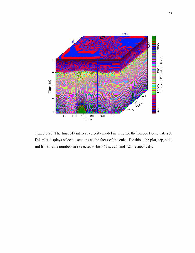
67
67
Figure 3.20. The final 3D interval velocity model in time for the Teapot Dome data set.
This plot displays selected sections as the faces of the cube. For this cube plot, top, side,
and front frame numbers are selected to be 0.65 s, 225, and 125, respectively.

68
68
Figure 3.21. The final 3D interval velocity model in depth after applying a time-to-depth
conversion to the velocity model shown in Fig. 3.20. This plot displays selected sections
as the faces of the cube. For this cube plot, top, side, and front frame numbers are
selected to be 3510 ft, 225, and 125, respectively.

69
69
Figure 3.22. The final slowness model in depth that is used as an input for post-stack
depth migration. This plot displays selected sections as the faces of the cube. For this
cube plot, top, side, and front frame numbers are selected to be 3510 ft, 225, and 125,
respectively.

70
70
Figure 3.23. The 3D post-stack time-migrated image of the Teapot Dome data set using
the Stolt’s method. This plot displays selected sections as the faces of the cube. For this
cube plot, top, side, and front frame numbers are selected to be 0.65 s, 225, and 125,
respectively.
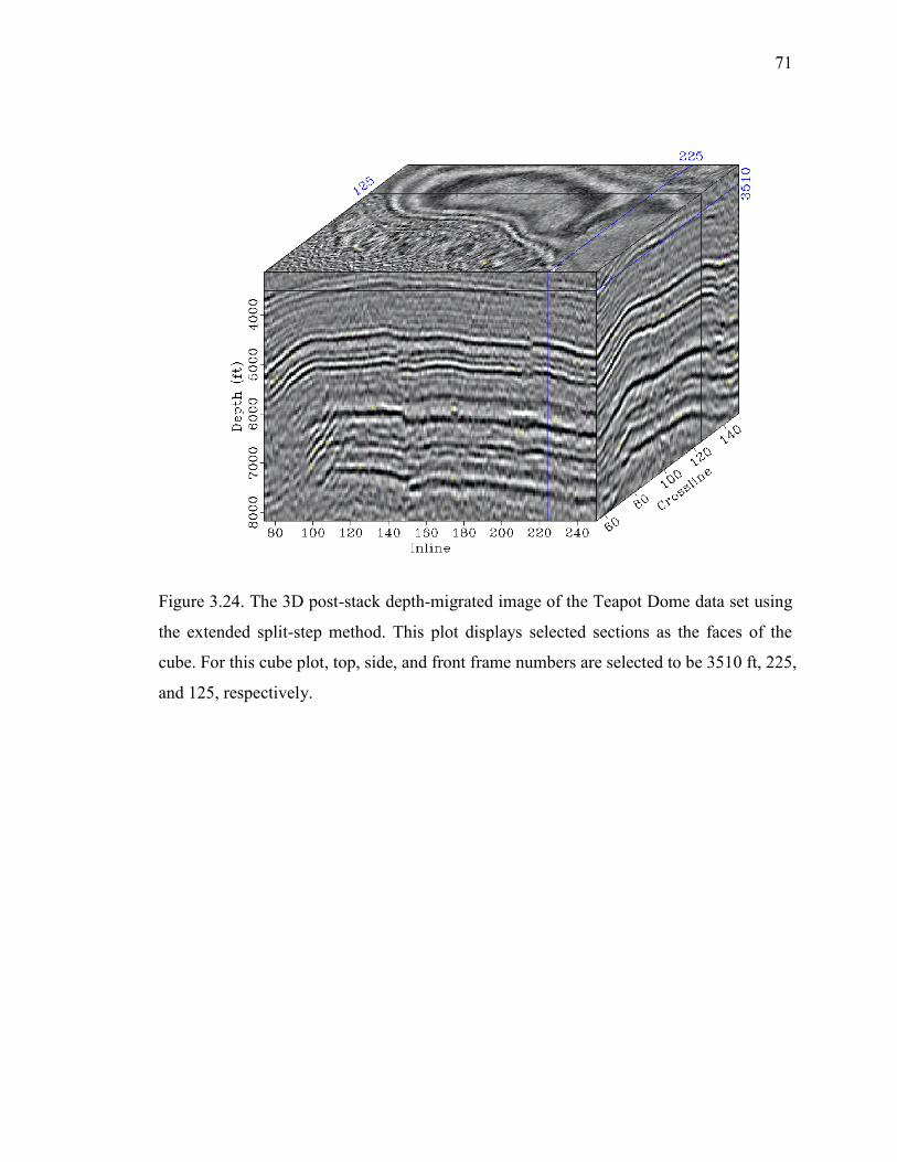
71
71
Figure 3.24. The 3D post-stack depth-migrated image of the Teapot Dome data set using
the extended split-step method. This plot displays selected sections as the faces of the
cube. For this cube plot, top, side, and front frame numbers are selected to be 3510 ft, 225,
and 125, respectively.

72
72
Figure 3.25. The 3D seismic image after applying a depth-to-time conversion to the
image shown in Fig. 3.24. This plot displays selected sections as the faces of the cube.
For this cube plot, top, side, and front frame numbers are selected to be 0.65 s, 225, and
125, respectively.

73
73
Figure 3.26. The 3D time-migrated image after applying f-x deconvolution to the image
shown in Fig. 3.23. This plot displays selected sections as the faces of the cube. For this
cube plot, top, side, and front frame numbers are selected to be 0.65 s, 225, and 125,
respectively.

74
74
Figure 3.27. The 3D seismic image after applying f-x deconvolution to the image shown
in Fig. 3.25. This plot displays selected sections as the faces of the cube. For this cube
plot, top, side, and front frame numbers are selected to be 0.65 s, 225, and 125,
respectively.

75
APPENDICES

75
75
Appendix A Additional results for the horizontal components of station SFIN
In this Appendix, the processed auto-correlations for the horizontal components (East and
North) of station SFIN are given.
Figure A.1. The processed auto-correlations for the horizontal component (E) of station
SFIN. a) is the hourly auto-correlations for the day of May 13, 2012 and the 1-day stack,
b) is the daily auto-correlation stacks for one month for May 2012 and the 1-month stack,
and c) is the monthly auto-correlation stacks for one year from January to December
2012 and the 1-year stack. d) A synthetic waveform derived from an average crustal
model derived from CRUST 1.0 for the location of station SFIN. An AGC and an offset
of source and receiver locations for the modeling are used to enhance the SmS arrival.
The arrows show the inferred PmP and SmS arrival times from the crustal model.

76
76
Figure A.2. The processed auto-correlations for the horizontal component (N) of station
SFIN. a) is the hourly auto-correlations for the day of May 13, 2012 and the 1-day stack,
b) is the daily auto-correlation stacks for one month for May 2012 and the 1-month stack,
and c) is the monthly auto-correlation stacks for one year from January to December
2012 and the 1-year stack. d) A synthetic waveform derived from an average crustal
model derived from CRUST 1.0 for the location of station SFIN. An AGC and an offset
of source and receiver locations for the modeling are used to enhance the SmS arrival.
The arrows show the inferred PmP and SmS arrival times from the crustal model.

77
77
Appendix B The scripts used to produce the figures in Chapter 3
In this Appendix, the Madagascar and MATLAB scripts used to produce the figures in
Chapter 3 are given.
Table B1. SConstruct script used to produce Figs 3.2, 3.3, and 3.4.
from rsf.proj import *
import math
# Convert the shot gathers and pre-processed CMP gathers from segy to rsf format.
Flow(['npr3_field.rsf','npr3_field_hdr.rsf',
'npr3_field.thdr','npr3_field.bhdr'],
'npr3_field.sgy',
'''
sfsegyread tfile=${TARGETS[1]} hfile=${TARGETS[2]} bfile=${TARGETS[3]}
''')
Flow(['npr3_gathers.rsf','npr3_gathers_hdr.rsf',
'npr3_gathers.thdr','npr3_gathers.bhdr'],
'npr3_gathers.sgy',
'''
sfsegyread tfile=${TARGETS[1]} hfile=${TARGETS[2]} bfile=${TARGETS[3]}
''')
# All shot coordinates.
Flow('sx','../fetch/npr3_field_hdr.rsf','dd type=float | headermath output="sx"')

78
78
Table B1 continued
Flow('sy','../fetch/npr3_field_hdr.rsf','dd type=float | headermath output="sy"')
Flow('sxsycoord',['sx','sy'],'cmplx ${SOURCES[1]} | math output="input*0.001"')
# All receiver coordinates.
Flow('gx','../fetch/npr3_field_hdr.rsf','dd type=float | headermath output="gx"')
Flow('gy','../fetch/npr3_field_hdr.rsf','dd type=float | headermath output="gy"')
Flow('gxgycoord',['gx','gy'],'cmplx ${SOURCES[1]} | math output="input*0.001"')
# Plot all the shot and receiver coordinates.
Plot('sxsycoord',
'''
graph symbol="+" title="(a)" label1="X" unit1="ft" label2="Y" unit2="ft" plotcol=5
labelsz=11
''')
Plot('gxgycoord',
'''
graph symbol="+" title="(b)" label1="X" unit1="ft" label2="Y" unit2="ft" plotcol=6
labelsz=11
''')
# Collect all shot and receiver coordinates in one plot and save it.
Result('sxsygxgycoord','sxsycoord gxgycoord','SideBySideAniso')
# Read and write one shot gather.
Flow(['fldr214.rsf','fldr214_hdr.rsf'],

79
79
Table B1 continued
['../fetch/npr3_field.rsf','../fetch/npr3_field_hdr.rsf'],
'''
sftahsort input=$SOURCE sort="fldr:214,214" verbose=1
| sftahwindow ns=2047
| sftahwrite verbose=1 mode=seq output=$TARGET
''',stdout=0,stdin=0)
# One shot coordinate.
Flow('sx1','fldr214_hdr.rsf','dd type=float | headermath output="sx"')
Flow('sy1','fldr214_hdr.rsf','dd type=float | headermath output="sy"')
Flow('sxsycoord1',['sx1','sy1'],'cmplx ${SOURCES[1]} | math output="input*0.001"')
# Receiver coordinates associated with the single shot.
Flow('gx1','fldr214_hdr.rsf','dd type=float | headermath output="gx"')
Flow('gy1','fldr214_hdr.rsf','dd type=float | headermath output="gy"')
Flow('gxgycoord1',['gx1','gy1'],'cmplx ${SOURCES[1]} | math output="input*0.001"')
# Plot one shot coordinate and its corresponding receiver coordinates.
Plot('sxsycoord1',
'''
graph symbol="+" title="(a)" label1="X" unit1="ft" label2="Y" unit2="ft" plotcol=5
plotfat=12 labelsz=11 symbolsz=8
min1=7.87573e+05 max1=8.09806e+05 min2=9.3841e+05 max2=9.76868e+05
''')

80
80
Table B1 continued
Plot('gxgycoord1',
'''
graph symbol="+" title="" label1="X" unit1="ft" label2="Y" unit2="ft" plotcol=6
labelsz=0
min1=7.87573e+05 max1=8.09806e+05 min2=9.3841e+05 max2=9.76868e+05
''')
# Create text boxes
Plot('r1',None,'box x0=9.868333 y0=7.230000 label="1" size=.3 xt=+0.5 yt=-0.3')
Plot('r2',None,'box x0=9.868333 y0=7.410000 label="2" size=.3 xt=+0.5 yt=+0.3')
Plot('r3',None,'box x0=9.208333 y0=7.590000 label="3" size=.3 xt=+0.5 yt=+0.3')
# Collect one shot coordinate and its corresponding receiver coordinates and in one plot
and save it.
Plot('sxsygxgycoord1','sxsycoord1 gxgycoord1 r1 r2 r3','Overlay')
# Read and write another shot gather.
Flow(['fldr825.rsf','fldr825_hdr.rsf'],
['../fetch/npr3_field.rsf','../fetch/npr3_field_hdr.rsf'],
'''
sftahsort input=$SOURCE sort="fldr:825,825" verbose=1
| sftahwindow ns=2047
| sftahwrite verbose=1 mode=seq output=$TARGET
''',stdout=0,stdin=0)

81
81
Table B1 continued
# One shot coordinate.
Flow('sx2','fldr825_hdr.rsf','dd type=float | headermath output="sx"')
Flow('sy2','fldr825_hdr.rsf','dd type=float | headermath output="sy"')
Flow('sxsycoord2',['sx2','sy2'],'cmplx ${SOURCES[1]} | math output="input*0.001"')
# Receiver coordinates associated with the single shot.
Flow('gx2','fldr825_hdr.rsf','dd type=float | headermath output="gx"')
Flow('gy2','fldr825_hdr.rsf','dd type=float | headermath output="gy"')
Flow('gxgycoord2',['gx2','gy2'],'cmplx ${SOURCES[1]} | math output="input*0.001"')
# Plot one shot coordinate and its corresponding receiver coordinates.
Plot('sxsycoord2',
'''
graph symbol="+" title="(b)" label1="X" unit1="ft" label2="Y" unit2="ft" plotcol=5
plotfat=12 labelsz=11 symbolsz=8
min1=7.87573e+05 max1=8.09806e+05 min2=9.3841e+05 max2=9.76868e+05
''')
Plot('gxgycoord2',
'''
graph symbol="+" title="" label1="X" unit1="ft" label2="Y" unit2="ft" plotcol=6
labelsz=0
min1=7.87573e+05 max1=8.09806e+05 min2=9.3841e+05 max2=9.76868e+05
''')

82
82
Table B1 continued
# Collect one shot coordinate and its corresponding receiver coordinates and in one plot
and save it.
Plot('sxsygxgycoord2','sxsycoord2 gxgycoord2','Overlay')
Result('sxsygxgycoord12','sxsygxgycoord1 sxsygxgycoord2','SideBySideAniso')
# Read the pre-processed CMP gathers.
Flow('gathers mask','../fetch/npr3_gathers.rsf ../fetch/npr3_gathers_hdr.rsf',
'intbin3 head=${SOURCES[1]} xkey=-1 mask=${TARGETS[1]}')
# Calculate the fold.
Flow('fold','mask','dd type=float | stack axis=1 norm=n')
# Save the plot of the fold map.
Result('fold',
'''
grey transp=n yreverse=n allpos=y color=j scalebar=y
label1="Crossline#" unit1="" label2="Inline#" unit2="" labelsz=6
wanttitle=n barlabel="Fold" barunit="" screenratio=1.3
''')
End()

83
83
Table B2. SConstruct script used to produce Figs 3.5 and 3.6.
from rsf.proj import *
# Create the mapped shot gathers.
Flow(['mappedfield.rsf','mappedfield_hdr.rsf'],
['../fetch/npr3_field.rsf','../fetch/npr3_field_hdr.rsf'],
'''
sftahread verbose=0 input=$SOURCE
| sftahwrite
verbose=1
label2="tracf" o2=1 n2=863 d2=1
label3="fldr" o3=14 n3=7 d3=100
output=$TARGET
''',stdout=0,stdin=0)
# Take a small portion of the shot gathers and save the result.
Plot('mappedfield',
'''
window max1=3 min2=440 max2=630 min3=214 max3=214 |
grey label1=Time unit1=s label2=Trace# unit2="" labelsz=6 wanttitle=no pclip=98
''')
# Create text boxes.

84
84
Table B2 continued
Plot('r1',None,'box x0=4.368333 y0=8.430000 label="1" size=.18 xt=+0.5 yt=+0.3')
Plot('r2',None,'box x0=8.288333 y0=8.430000 label="2" size=.18 xt=+0.5 yt=+0.3')
Plot('r3',None,'box x0=11.808333 y0=8.430000 label="3" size=.18 xt=+0.5 yt=+0.3')
# Collect and save the results in one plot.
Result('mappedfield_214','mappedfield r1 r2 r3','Overlay')
# Take a shot gather.
Flow('mappedfield_214_subset','mappedfield',
'''
window max1=2 min2=510 max2=570 min3=214 max3=214
''')
# Apply tpow to the shot gathers.
Flow('mappedfield_214_subset_tpow','mappedfield_214_subset','pow pow1=2')
# Extract a subset of shot gathers to test sftahagc.
Flow(['mappedfield_214_subset_agc.rsf','mappedfield_214_subset_agc_hdr.rsf'],
['../fetch/npr3_field.rsf','../fetch/npr3_field_hdr.rsf'],
'''
sftahsort verbose=1 input=${SOURCES[0]} sort='fldr:214,254,10 tracf'
| sftahwindow ns=2047

85
85
Table B2 continued
| sftahagc wagc=1.000 verbose=1
| sftahwrite verbose=1 label2="tracf" o2=1 n2=1063 d2=1 label3="fldr" o3=214 n3=5
d3=10 output=${TARGETS[0]} outheaders=${TARGETS[1]}
''',stdout=0,stdin=0)
# Plot the raw shot gather.
Plot('mappedfield_214_subset',
'''
grey label1=Time unit1=s label2=Trace# unit2= labelsz=14 titlesz=14 title="(a)"
pclip=90
''')
# Create a text box.
Plot('gr',None,'box x0=6.968333 y0=7.250000 label="ground roll" size=.45 xt=-2.2
yt=+1.5')
# Plot the raw shot gather with the text box.
Plot('mappedfield_214_subset_gr','mappedfield_214_subset gr','Overlay')
# Plot the shot gather in (a) with tpow.
Plot('mappedfield_214_subset_tpow',
'''
grey label1=Time unit1=s label2=Trace# unit2= labelsz=14 titlesz=14 title="(b)"
pclip=90
''')

86
86
Table B2 continued
# Plot the shot gather in (a) with AGC.
Plot('mappedfield_214_subset_agc',
'''
window min1=0 max1=2 min2=510 max2=570 min3=214 max3=214 |
grey label1=Time unit1=s label2=Trace# unit2= labelsz=14 titlesz=14 title="(c)"
pclip=90
''')
# Create text boxes.
Plot('art1',None,'box x0=3.648333 y0=8.580000 label="artifact" size=.45 xt=+0.35 yt=-
0.35')
Plot('art2',None,'box x0=11.098333 y0=8.580000 label="artifact" size=.45 xt=-0.35 yt=-
0.35')
Plot('mappedfield_214_subset_agc_art','mappedfield_214_subset_agc art1
art2','Overlay')
# Collect and save the results in one plot.
Result('mappedfield_all','mappedfield_214_subset_gr mappedfield_214_subset_tpow
mappedfield_214_subset_agc_art','SideBySideAniso')
End()

87
87
Table B3. SConstruct script used to produce Fig. 3.7.
from rsf.proj import *
# Extract a subset of shot gathers for AGC and mute.
Flow(['agcmuteshot.rsf','agcmuteshot_hdr.rsf'],
['../fetch/npr3_field.rsf','../fetch/npr3_field_hdr.rsf'],
'''
sftahsort verbose=1 input=${SOURCES[0]} sort='fldr:214,254,10 tracf'
| sftahwindow ns=2047
| sftahagc wagc=1.000 verbose=1
| sftahmute tmute=-.200,-.050,.200,2.30 xmute=0,880,1760,18000 ntaper=80
| sftahwrite verbose=1 label2="tracf" o2=1 n2=1063 d2=1 label3="fldr" o3=214
n3=5 d3=10 output=${TARGETS[0]} outheaders=${TARGETS[1]}
''',stdout=0,stdin=0)
# Extract a subset of shot gathers for mute, spiking deconvolution and AGC.
Flow(['mutepefagcshot.rsf','mutepefagcshot_hdr.rsf'],
['../fetch/npr3_field.rsf','../fetch/npr3_field_hdr.rsf'],
'''
sftahsort verbose=0 input=${SOURCES[0]} sort='fldr:214,254,10 tracf'
| sftahmute tmute=-.200,-.050,.200,2.30 xmute=0,880,1760,18000 ntaper=80
| sftahpef verbose=1 minlag=.002 maxlag=.1 pnoise=.01 mincorr=0 maxcorr=3
| sftahagc wagc=1.000 verbose=1

88
88
Table B3 continued
| sftahwrite verbose=1 label2="tracf" o2=1 n2=1063 d2=1 label3="fldr" o3=214 n3=5
d3=10 output=${TARGETS[0]} outheaders=${TARGETS[1]}
''',stdout=0,stdin=0)
# Extract a subset of shot gathers for mute, spiking deconvolution, AGC, and statics.
Flow(['mutepefagcstaticshot.rsf','mutepefagcstaticshot_hdr.rsf'],
['../fetch/npr3_field.rsf','../fetch/npr3_field_hdr.rsf'],
'''
sftahsort verbose=0 input=${SOURCES[0]} sort='fldr:214,254,10 tracf'
| sftahmute tmute=-.200,-.050,.200,2.30 xmute=0,880,1760,18000 ntaper=80
| sftahpef verbose=1 minlag=.002 maxlag=.1 pnoise=.01 mincorr=0 maxcorr=3
| sftahagc wagc=1.000 verbose=1 | sftahstatic sign=-1
| sftahwrite verbose=1 label2="tracf" o2=1 n2=1063 d2=1 label3="fldr" o3=214 n3=5
d3=10 output=${TARGETS[0]} outheaders=${TARGETS[1]}
''',stdout=0,stdin=0)
# Plot the shot gather for shot index 214 after AGC and mute.
Plot('agcmuteshotzoom','agcmuteshot',
'''
sfwindow min1=0 max1=2 min2=510 max2=570 min3=214 max3=214 \
| sfgrey label1="Time" unit1="s" label2="Trace#" unit2="" title="(a)" labelsz=14
titlesz=14 pclip=90 transp=y yreverse=y
''')

89
89
Table B3 continued
# Plot the shot gather for shot index 214 after mute, spiking deconvolution and AGC.
Plot('mutepefagcshotzoom','mutepefagcshot',
'''
sfwindow min1=0 max1=2 min2=510 max2=570 min3=214 max3=214 \
| sfgrey label1="Time" unit1="s" label2="Trace#" unit2="" title="(b)" labelsz=14
titlesz=14 \
pclip=90 transp=y yreverse=y
''')
# Plot the shot gather for shot index 214 after mute, spiking deconvolution, AGC, and
static corrections.
Plot('mutepefagcstaticshotzoom','mutepefagcstaticshot',
'''
sfwindow min1=0 max1=2 min2=510 max2=570 min3=214 max3=214 \
| sfgrey label1="Time" unit1="s" label2="Trace#" unit2="" title="(c)" labelsz=14
titlesz=14 \
pclip=90 transp=y yreverse=y
''')
# Collect and save the results in one plot.
Result('agcmutepefstaticshot','agcmuteshotzoom mutepefagcshotzoom
mutepefagcstaticshotzoom','SideBySideAniso')
End()

90
90
Table B4. SConstruct script used to produce Figs 3.8, 3.9, and 3.10.
from rsf.proj import *
# Read the pre-processed CMP gathers.
Flow('gathers mask','../fetch/npr3_gathers.rsf ../fetch/npr3_gathers_hdr.rsf',
'intbin3 head=${SOURCES[1]} xkey=-1 mask=${TARGETS[1]}')
# Take the offset information from the headers.
Flow('offset','../fetch/npr3_gathers_hdr.rsf',
'window n1=1 f1=11 squeeze=n | intbin3 head=$SOURCE xkey=-1 | dd type=float')
Flow('mask3','mask','spray axis=1 n=1')
# Velocity analysis at one CMP for the midpoint of crossline= 120 and inline=160.
Flow('gather1','gathers','window n3=1 n4=1 f3=120 f4=160')
Flow('offset1','offset', 'window n3=1 n4=1 f3=120 f4=160')
Flow('mask1','mask3', 'window n3=1 n4=1 f3=120 f4=160')
# Plot one CMP gather.
Plot('gather1','gather1 offset1',
'''
window max1=2.0 max2=25 |
wiggle xpos=${SOURCES[1]} transp=y poly=y yreverse=y title="(a)"
label2=Offset unit2=ft wherexlabel=t wheretitle=b grid=n labelsz=14 titlesz=14
''')

91
91
Table B4 continued
# Apply a window to the CMP gather.
Flow('gather1win','gather1','window max1=2.0')
# Velocity analysis.
Flow('vscan1','gather1 offset1 mask1',
'vscan offset=${SOURCES[1]} mask=${SOURCES[2]} v0=9000 nv=101 dv=100
semblance=y half=n nb=10')
# Apply a window to the velocity scan.
Flow('vscan1win','vscan1','window max1=2.0')
# Pick the velocities manually from the velocity scan.
Flow('manualpicks.asc','vscan1win','ipick grey color=j allpos=y title="Velocity Scan"
unit2=ft/s labelsz=10 titlesz=10')
# Plot the windowed velocity scan.
Plot('vscan1win',
'''
grey color=j allpos=y title="(b)" unit2=ft/s labelsz=14 titlesz=14
''')

92
92
Table B4 continued
# tnmo and vnmo pairs picked by user.
tnmo1=(0.0,0.653913,0.817391,0.935652,1.03652,1.21739,1.77739)
vnmo1=(9026.08,10981.7,11255.5,11425,11672.8,12807,15179.9)
# Write user's tnmo and vnmo pairs to a file.
Flow('vnmo1.asc',None,
'''
echo %s n1=%d n2=2 data_format=ascii_float in=$TARGET
''' % (' '.join(map(str,tnmo1)+map(str,vnmo1)),len(tnmo1)))
# Interpolate the user's tnmo and vnmo pairs.
Flow('vnmo1','vnmo1.asc gather1win',
'dd form=native | linear pattern=${SOURCES[1]} rect=5 niter=100')
# Read the contractor's average velocity to use for NMO correction.
Flow('vrms_avg','v_rms_avg.asc','dd form=native | put d1=0.002')
# Plot average RMS velocities used for NMO correction.
Plot('vrms_avg',
'''
window min1=0 max1=2 |
graph yreverse=y transp=y pad=n plotcol=5 plotfat=8 wanttitle=n wherexlabel=t

93
93
Table B4 continued
label1=Time unit1=s label2='Average RMS Velocity' unit2=ft/s labelsz=0
screenratio=1.5 min2=9000 max2=15500
''')
# Plot the manually picked RMS velocities for comparison.
Plot('vnmopicked’,’vnmo1',
'''
window max1=2 | graph yreverse=y transp=y pad=n plotcol=6 plotfat=8 wanttitle=n
wherexlabel=t label1=Time unit1=s label2='RMS Velocity' unit2=ft/s labelsz=6
screenratio=1.5 min2=9000 max2=15300
''')
# Read the contractor's interpolated RMS velocities for the same midpoint location.
Flow('vcont','../velocity_model/Vrms3D.rsf','window min2=120 max2=120 min3=160
max3=160')
# Plot the contractor's interpolated RMS velocities.
Plot('vcont',
'''
window min1=0 max1=2 |
graph yreverse=y transp=y pad=n plotcol=3 plotfat=8 wanttitle=n wherexlabel=t
dash=1
label1=Time unit1=s label2='Average RMS Velocity' unit2=ft/s labelsz=0
screenratio=1.5 min2=9000 max2=15500
''')

94
94
Table B4 continued
# Overlay the plots and save it.
Result('vnmos','vnmopicked vcont vrms_avg','Overlay')
# Plot the picked RMS velocities for the velocity scan.
Plot('vnmo1',
'''
graph yreverse=y transp=y pad=n plotcol=7 plotfat=13 wanttitle=n wherexlabel=t
label1=Time unit1=s label2='User RMS Velocity' unit2=ft/s labelsz=0 min2=9000
max2=19000
''')
# Spray the pairs.
Flow('vnmo3',' vrms_avg ','spray axis=1 n=1 | spray axis=3 n=188 | spray axis=4 n=345')
Flow('mask3','mask','spray axis=1 n=1')
# Apply NMO correction.
Flow('nmo','gathers offset vnmo3 mask3',
'''
nmo offset=${SOURCES[1]} half=n velocity=${SOURCES[2]}
mask=${SOURCES[3]}
''',split=[4,345])

95
95
Table B4 continued
# Take one CMP from NMO corrected gathers.
Flow('gather1nmo','nmo','window n3=1 n4=1 f3=120 f4=160')
# Plot the NMO corrected CMP gather.
Plot('gather1nmo','gather1nmo offset1',
'''
window max1=2.0 max2=25 |
wiggle xpos=${SOURCES[1]} transp=y poly=y yreverse=y title="(c)"
label2=Offset unit2=ft wherexlabel=t wheretitle=b grid=n labelsz=14 titlesz=14
''')
# Overlay the plots of velocity scan and user's tnmo-vnmo pairs.
Plot('vscan1pickwin','vscan1win vnmo1','Overlay')
# Collect the plots in a figure and save it.
Result('cmpvscan1picknmo','gather1 vscan1pickwin gather1nmo','SideBySideAniso')
# Stack the data.
Flow('stackcube','nmo','stack',split=[4,345],reduce='cat axis=3')
# Transpose the stack.
Flow('stackcubet','stackcube','transp plane=23 memsize=1000')

96
96
Table B4 continued
# Plot the stacked data and save it.
Result('stackcubet',
'''
window min1=0.6 max1=1.3 min2=75 max2=250 min3=55 max3=150 |
byte gainpanel=all pclip=96 |
grey3 wanttitle=n frame1=25 frame2=150 frame3=70 flat=n point1=0.7 point2=0.7
label1=Time unit1=s label2=Inline unit2= label3=Crossline unit3= labelsz=6
''')
# Bandpass filtering.
Flow('stackcube_filter','stackcubet','bandpass flo=12 fhi=90')
# Plot the bandpass filtered data and save it.
Result('stackcube_filter',
'''
window min1=0.6 max1=1.3 min2=75 max2=250 min3=55 max3=150 |
byte gainpanel=all pclip=96 |
grey3 wanttitle=n frame1=25 frame2=150 frame3=70 flat=n point1=0.7 point2=0.7
label1=Time unit1=s label2=Inline unit2= label3=Crossline unit3= labelsz=6
''')
End()

97
97
Table B5. SConstruct script used to produce Figs 3.11, 3.12, 3.13, 3.14, and 3.15.
from rsf.proj import *
# Inline 225 stacked section after tpow, mute, and AGC.
Flow(['tpowmuteagcstack225.rsf','tpowmuteagcstack225_hdr.rsf'],
['../fetch/npr3_field.rsf','../fetch/npr3_field_hdr.rsf'],
'''
sftahsort verbose=1 input=${SOURCES[0]} sort='iline:225,225 xline offset'
| sftahwindow ns=2047
| sftahgain tpow=2
| sftahmute tmute=0.0,3.3 xmute=0,18000 ntaper=40
| sftahagc wagc=1.000 verbose=1
| sftahnmo verbose=1
tnmo=0.00,.479,.637,.792,.877,1.009,1.104,1.19458,1.615,3.010
vnmo=9132.86,10553.29,10921.60,10791.97,11074.19,11649.54,11807.96,12325.03,144
10.47,17216.64
| sftahstack key=iline,xline verbose=1 ntaper=40
| sftahwrite verbose=1 label2="xline" o2=1 n2=188 d2=1
label3="iline" o3=225 n3=1 d3=1 output=${TARGETS[0]}
outheaders=${TARGETS[1]}
''',stdout=0,stdin=0)

98
98
Table B5 continued
Result('tpowmuteagcstack225',
'''
window min1=0.5 max1=2.0 min2=55 max2=150
| wiggle label2="Crossline#" wanttitle=n grid=n transp=y poly=y yreverse=y
wherexlabel=t labelsz=6
''')
# Inline 225 stacked section after tpow, mute, spiking decon, and AGC.
Flow(['tpowmutepefagcstack225.rsf','tpowmutepefagcstack225_hdr.rsf'],
['../fetch/npr3_field.rsf','../fetch/npr3_field_hdr.rsf'],
'''
sftahsort verbose=1 input=${SOURCES[0]} sort='iline:225,225 xline offset'
| sftahwindow ns=2047
| sftahgain tpow=2
| sftahmute tmute=-0.300,3.0 xmute=0,18000 ntaper=75
| sftahpef verbose=1 minlag=.002 maxlag=.1 pnoise=.01 mincorr=0 maxcorr=3
| sftahagc wagc=1.000 verbose=1
| sftahmute tmute=0.0,3.3 xmute=0,18000 ntaper=75
| sftahnmo verbose=1 tnmo=0.00,.479,.637,.792,.877,1.009,1.104,1.19458,1.615,3.010
vnmo=9132.86,10553.29,10921.60,10791.97,11074.19,11649.54,11807.96,12325.03,144
10.47,17216.64

99
99
Table B5 continued
| sftahstack key=iline,xline verbose=1 ntaper=75
| sftahwrite verbose=1 label2="xline" o2=1 n2=188 d2=1
label3="iline" o3=225 n3=1 d3=1 output=${TARGETS[0]}
outheaders=${TARGETS[1]}
''',stdout=0,stdin=0)
Result('tpowmutepefagcstack225',
'''
window min1=0.5 max1=2.0 min2=55 max2=150
| wiggle label2="Crossline#" wanttitle=n grid=n transp=y poly=y yreverse=y
wherexlabel=t labelsz=6
''')
# Inline 225 stacked section after tpow, mute, AGC, and statics.
Flow(['tpowmuteagcstaticstack225.rsf','tpowmuteagcstaticstack225_hdr.rsf'],
['../fetch/npr3_field.rsf','../fetch/npr3_field_hdr.rsf'],
'''
sftahsort verbose=1 input=${SOURCES[0]} sort='iline:225,225 xline offset'
| sftahwindow ns=2047
| sftahgain tpow=2
| sftahmute tmute=0.0,3.3 xmute=0,18000 ntaper=40

100
100
Table B5 continued
| sftahagc wagc=1.000 verbose=1
| sftahstatic sign=-1
| sftahnmo verbose=1
tnmo=0.00,.479,.637,.792,.877,1.009,1.104,1.19458,1.615,3.010
vnmo=9132.86,10553.29,10921.60,10791.97,11074.19,11649.54,11807.96,12325.03,144
10.47,17216.64
| sftahstack key=iline,xline verbose=1 ntaper=40
| sftahwrite verbose=1 label2="xline" o2=1 n2=188 d2=1 label3="iline" o3=225
n3=1 d3=1 output=${TARGETS[0]} outheaders=${TARGETS[1]}
''',stdout=0,stdin=0)
Result('tpowmuteagcstaticstack225',
'''
window min1=0.5 max1=2.0 min2=55 max2=150
| wiggle label2="Crossline#" wanttitle=n grid=n transp=y poly=y yreverse=y
wherexlabel=t labelsz=6
''')
# Inline 225 stacked section after tpow, mute, spiking decon, AGC, and statics.
Flow(['tpowmutepefagcstaticstack225.rsf','tpowmutepefagcstaticstack225_hdr.rsf'],
['../fetch/npr3_field.rsf','../fetch/npr3_field_hdr.rsf'],
'''
sftahsort verbose=1 input=${SOURCES[0]} sort='iline:225,225 xline offset'

101
101
Table B5 continued
| sftahwindow ns=2047
| sftahgain tpow=2
| sftahmute tmute=-0.300,3.0 xmute=0,18000 ntaper=75
| sftahpef verbose=1 minlag=.002 maxlag=.1 pnoise=.01 mincorr=0 maxcorr=3
| sftahagc wagc=1.000 verbose=1
| sftahmute tmute=0.0,3.3 xmute=0,18000 ntaper=75
| sftahstatic sign=-1
| sftahnmo
verbose=1
tnmo=0.00,.479,.637,.792,.877,1.009,1.104,1.19458,1.615,3.010
vnmo=9132.86,10553.29,10921.60,10791.97,11074.19,11649.54,11807.96,12325.03,144
10.47,17216.64
| sftahstack key=iline,xline verbose=1 ntaper=75
| sftahwrite verbose=1 label2="xline" o2=1 n2=188 d2=1 label3="iline" o3=225 n3=1
d3=1 output=${TARGETS[0]} outheaders=${TARGETS[1]}
''',stdout=0,stdin=0)
Result('tpowmutepefagcstaticstack225',
'''
window min1=0.5 max1=2.0 min2=55 max2=150
| wiggle label2="Crossline#" wanttitle=n grid=n transp=y poly=y yreverse=y
wherexlabel=t labelsz=6

102
102
Table B5 continued
''')
# Plot the inline 225 stacked section obtained from the contractor's pre-processed CMP
gathers and save it for comparison.
Result('tpowmutepefagcstack225_cont','../nmostack/stackcube.rsf',
'''
window min1=0.5 max1=2.0 min2=55 max2=150 min3=225 max3=225 |
scale rscale=-1.0 |
wiggle label2="Crossline#" wanttitle=n grid=n transp=y poly=y yreverse=y
wherexlabel=t labelsz=6
''')
End()

103
103
Table B6. MATLAB script used to produce Fig. 3.16.
clc; clear all;
% Read the header information using the CREWES software.
% [tracehead,texthead,binaryhead,extendedhead]=SEGY_read;
% hdr = SEGY_getHeader(texthead,'header');
% hdrcdpx = SEGY_getHeader(tracehead,'cdpx');
% hdrcdpy = SEGY_getHeader(tracehead,'cdpy');
% hdrcdp = SEGY_getHeader(tracehead,'cdp');
% hdriline = SEGY_getHeader(tracehead,'iline');
% hdrxline = SEGY_getHeader(tracehead,'xline');
% Assign the contractor’s time (in ms) and post DMO RMS (in ft) velocity pairs.
tv1=[0 8874.3
571.23 10265.44
863.1 10995.03
992.36 11235.75
1107.02 11626.8
1240.44 12252.14
1392.63 13178.23
1922.17 14513.85
3010 16693.72];

104
104
Table B6 continued
tv2=[0 8842.17
314.8 9697.7
640.03 10576.45
825.57 10917.55
963.17 11064.88
1052.81 11106.86
1182.07 11876.82
1286.31 12171.38
1530.23 13387.92
1851.29 14561.19
2927.03 16650.59
3010 16740.01];
tv3=[0 8852.84
281.45 9655.81
731.76 10742.94
917.3 10969.02
1013.2 11021.23
1163.31 11840.42
1302.99 12325.03
1724.11 13937.65
2334.95 15981.86
3010 16954.96];

105
105
Table B6 continued
tv4=[0 8917.69
281.45 9641.97
583.74 10469.54
715.08 10943.19
867.27 10623.22
961.08 10841.68
1140.38 11527.3
1307.16 12216.18
1690.76 14561.19
2074.36 15736.06
2666.43 16722.18
3010 17117.68];
tv5=[0 9144.62
571.23 10244.26
698.4 10694.57
917.3 11100.96
1031.97 11467.61
1144.54 12145.2
1313.41 12800.43
1974.29 15558.97
3010 17206.82];

106
106
Table B6 continued
tv6=[0 9029.02
406.53 10116.87
719.25 10718.67
898.54 10881.67
990.27 11170.75
1157.05 11939.45
1305.07 12145.2
1826.27 14755.28
2908.27 16794.7
3010 16901.72];
tv7=[0 9082.99
729.67 10767.37
877.69 10841.68
981.93 10995.03
1152.88 11775.76
1298.82 12180.53
1834.61 14776.57
3010 16997.43];

107
107
Table B6 continued
tv8=[0 9068.31
400.28 10019.63
712.99 10791.97
892.29 11021.23
1186.24 12075.44
1609.45 13702.32
2088.95 15311.14
3010 16873.4];
tv9=[0 8874.3
266.85 9351.76
504.52 9961
683.81 10462.16
794.3 10861.87
996.53 11155.08
1088.26 11527.3
1296.73 12704.56
1384.29 13002.05
1895.07 14608.99
3010 16797.06];

108
108
Table B6 continued
tv10=[0 8906.79
617.1 10395.33
783.88 10816.74
921.47 11210.01
1029.88 11379.78
1163.31 12088.88
1317.58 12800.43
1515.64 13425.05
1957.61 15061.56
2939.54 16868.17
3010 16937.01];
tv11=[0 8885.09
262.68 9614.47
558.72 10469.54
706.74 11085.81
856.84 10901.58
963.17 10961.97
1211.26 12227.33
1738.71 14283.88
2939.54 16868.17
3010 16937.01];

109
109
Table B6 continued
tv12=[0 8961.73
435.72 10181.3
519.11 10505.09
644.2 10670.63
844.34 10961.97
1077.83 11825.52
1242.53 12399.92
1594.86 14151.04
1742.88 15114.48
3010 17330.18];
tv13=[0 8995.18
577.48 10577.28
660.88 10816.74
833.91 10841.68
936.07 11074.19
1082 11906.17
1238.36 12590.76
1715.77 14855.29
3010 17246.51];

110
110
Table B6 continued
tv14=[0 9017.7
658.79 10764.47
846.42 11064.88
1054.9 11906.17
1232.11 12580.03
1830.44 14706.03
3010 16967.51];
tv15=[0 9086.27
660.88 10961.97
840.17 11106.86
940.24 11235.75
1056.98 11928.78
1232.11 12459.1
1624.04 14239.19
1851.29 14957.36
3010 17065.17];
tv16=[0 9097.85
596.25 10861.87
681.72 11128.04

111
111
Table B6 continued
850.59 11155.08
954.83 11265.75
1092.42 12061.75
1265.46 12704.56
2036.83 15501.26
3010 17075.28];
tv17=[0 9063.24
287.7 9783.13
556.64 10469.54
740.1 10921.6
888.12 10917.55
977.76 11210.01
1119.53 12110.17
1273.8 12610.82
1953.44 15009.19
3010 16918.3];
tv18=[0 8961.73
529.53 10246.97
923.56 11149.33

112
112
Table B6 continued
1094.51 11507.57
1225.85 12006.87
1407.23 12800.43
1840.86 14608.99
2149.41 15331.9
3010 16787.81];
tv19=[0 9017.7
262.68 9655.81
550.38 10308.2
694.23 10881.67
869.35 11127.92
977.76 11437.77
1123.7 11955.02
1305.07 12865.55
1703.27 14329
1984.71 15114.48
2889.51 16794.7
3010 16923.53];
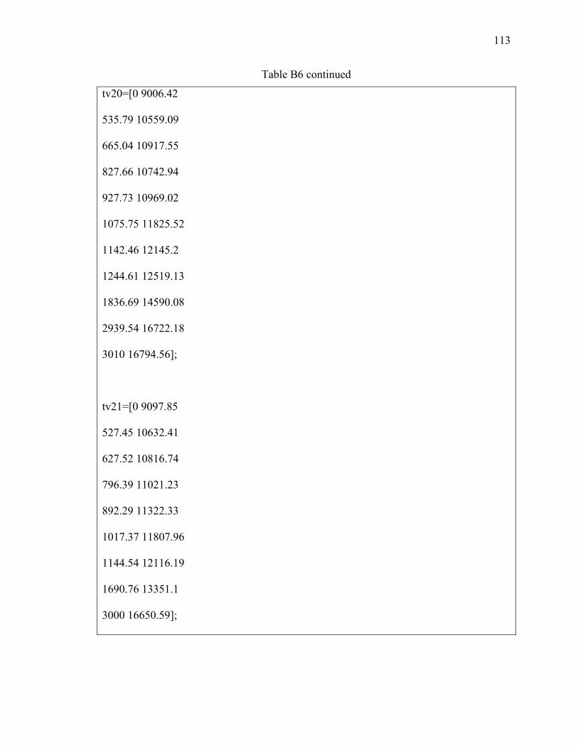
113
113
Table B6 continued
tv20=[0 9006.42
535.79 10559.09
665.04 10917.55
827.66 10742.94
927.73 10969.02
1075.75 11825.52
1142.46 12145.2
1244.61 12519.13
1836.69 14590.08
2939.54 16722.18
3010 16794.56];
tv21=[0 9097.85
527.45 10632.41
627.52 10816.74
796.39 11021.23
892.29 11322.33
1017.37 11807.96
1144.54 12116.19
1690.76 13351.1
3000 16650.59];

114
114
Table B6 continued
tv22=[0 9029.02
627.52 10623.22
840.17 11021.23
1019.46 11902.71
1100.76 12216.18
1227.94 12865.55
3010 17436.33];
tv23=[0 9132.86
617.09 10764.47
796.39 10941.73
913.13 11235.75
1027.8 11902.71
1196.66 12580.03
1767.89 14513.85
3010 16982.86];
tv24=[0 9097.85
489.92 10434.35
635.86 10842.18
817.23 11064.88
917.3 11210.01

115
115
Table B6 continued
1148.71 12199.26
1215.43 12474.79
1784.57 14657.27
3010 17025.09];
tv25=[0 9063.24
354.41 10069.34
650.45 10767.37
821.4 10767.37
927.73 10969.02
1052.81 11531.12
1215.43 12341.58
1940.93 15061.56
3010 16969.86];
tv26=[0 9097.85
650.45 10767.37
829.74 11044.06
961.08 11324.2
1069.49 11649.54
1252.95 12513.09

116
116
Table B6 continued
1507.3 13908.99
1924.25 15241.13
3010 17100.56];
tv27=[0 9086.27
523.28 10462.16
669.21 10742.94
865.18 11074.19
969.42 11100.96
1086.17 11438.1
1248.78 12288.42
1813.76 15009.19
3010 17157.04];
tv28=[0 9097.85
660.88 10816.74
886.03 10995.03
981.93 11155.08
1107.02 11743.82
1207.09 12110.17
1722.03 14561.19
2593.47 16671.46
3010 17160.37];

117
117
Table B6 continued
tv29=[0 8995.18
592.08 10329.78
710.91 10791.97
883.95 10841.68
996.53 11350.94
1234.19 12180.53
1617.79 13773.72
3000 16650.59];
tv30=[0 9216.15
256.43 9976.26
452.4 10395.33
656.71 10917.55
892.29 11127.92
1079.92 11851.09
1707.44 14064.52
3010 16879.72];
tv31=[0 9204.11
391.94 10382.23
675.47 11085.81
873.52 11213.95
1056.98 11578.66

118
118
Table B6 continued
1273.8 12832.87
1653.23 14283.88
3010 17088.15];
tv32=[0 9216.15
496.18 10783.74
650.45 11170.75
821.4 11257.67
936.07 11437.77
1148.71 12312.72
1646.98 14513.85
2022.24 15501.26
3010 17098.02];
tv33=[0 9168.27
366.92 10365.03
631.69 11182.44
823.49 11257.67
894.37 11379.78
1023.63 11851.09
1709.52 14151.04
3010 16916.72];

119
119
Table B6 continued
tv34=[0 9063.24
585.82 10599.76
788.05 10881.67
906.88 11128.04
1042.39 11851.09
1200.83 12519.13
1713.69 13937.65
2232.8 15617.34
3010 16846.98];
tv35=[0 9040.38
617.09 10803.11
773.45 11085.81
896.46 11064.88
1038.22 11955.02
1213.34 12459.1
1661.57 14420.54
1828.35 14855.29
3010 17050.31];

120
120
Table B6 continued
tv36=[0 9051.79
300.21 9885.71
625.43 10742.94
823.49 11047.61
936.07 11100.96
1090.34 12284.05
1217.51 12610.82
1945.1 15601.14
3010 17276.08];
tv37=[0 9063.24
304.38 9915.62
667.13 11074.19
831.83 11021.23
929.81 11182.44
1059.07 12110.17
1213.34 12551.74
1682.42 14239.19
2097.29 15558.97
3010 17017.63];

121
121
Table B6 continued
tv38=[0 9097.85
602.5 10982.32
858.93 11210.01
952.74 11408.83
1065.32 12143.69
1227.94 12549.47
2030.58 15444.18
3010 17050.01];
tv39=[0 9109.47
250.17 9915.62
658.79 11127.92
861.01 11047.61
1054.9 11557.5
1590.69 13504.59
2086.86 15276.67
3010 16855.06];
tv40=[0 9086.27
373.18 10244.26
619.18 11085.81
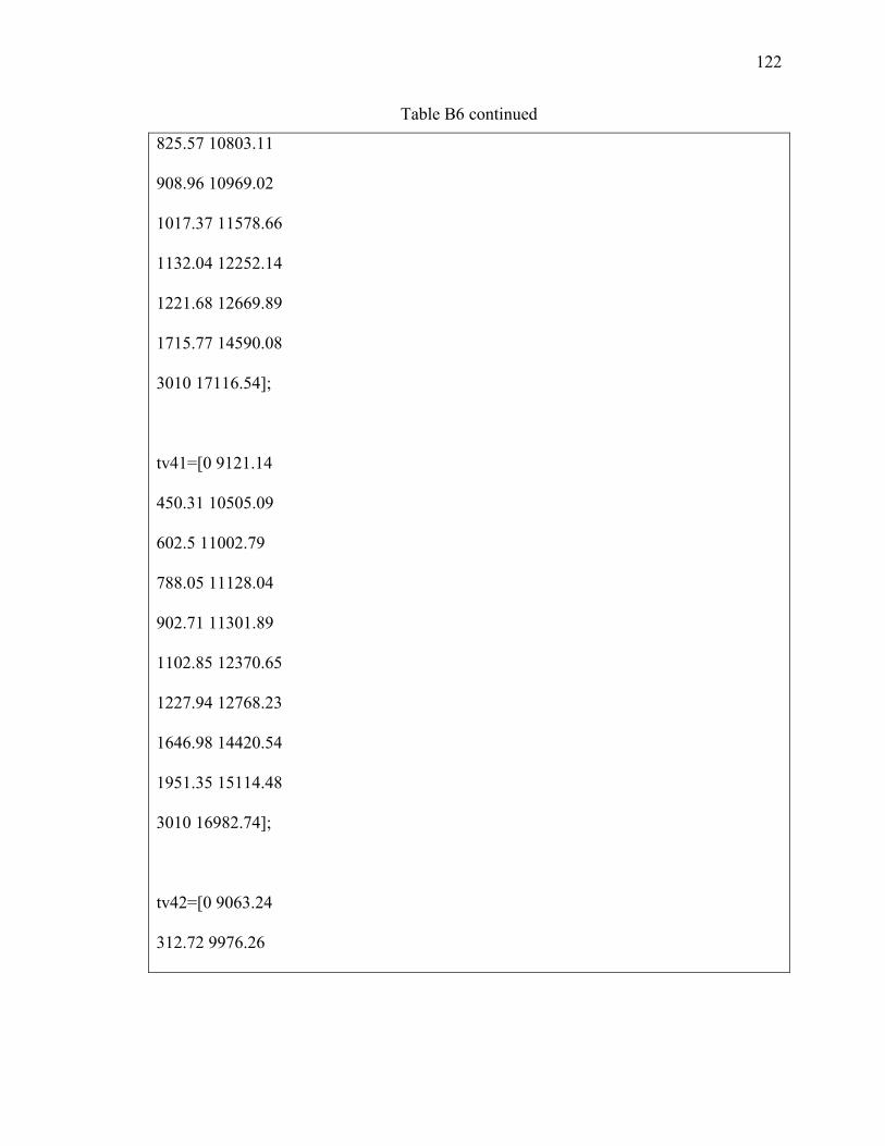
122
122
Table B6 continued
825.57 10803.11
908.96 10969.02
1017.37 11578.66
1132.04 12252.14
1221.68 12669.89
1715.77 14590.08
3010 17116.54];
tv41=[0 9121.14
450.31 10505.09
602.5 11002.79
788.05 11128.04
902.71 11301.89
1102.85 12370.65
1227.94 12768.23
1646.98 14420.54
1951.35 15114.48
3010 16982.74];
tv42=[0 9063.24
312.72 9976.26

123
123
Table B6 continued
600.42 10694.57
792.22 11106.86
900.63 11265.75
1027.8 12088.88
1200.83 12580.03
1920.08 15167.97
3010 17065.71];
tv43=[0 9097.85
594.16 11023.37
794.3 11100.96
904.79 11210.01
1040.31 11680.72
1113.27 11981.44
1215.43 12710.03
1913.83 15676.36
3010 17366.53];
tv44=[0 9040.38
469.08 10416.89
667.13 10969.02

124
124
Table B6 continued
819.32 10841.68
1044.47 12110.17
1219.6 12791.45
1740.79 14755.28
1936.76 15444.18
3010 17197.45];
tv45=[0 9086.27
546.21 10650.97
810.98 11002.79
902.71 11182.44
1046.56 12180.53
1205 12800.43
1803.34 15167.97
3010 17258.37];
tv46=[0 9063.24
283.53 9960.89
627.52 10943.19
831.83 11210.01
1034.05 11928.78

125
125
Table B6 continued
1219.6 12580.03
1644.89 14151.04
2093.12 15387.73
3010 16915.14];
tv47=[0 9017.7
258.51 9812.11
481.58 10767.37
585.82 11044.06
675.47 11085.81
810.98 11127.92
911.05 11437.77
1017.37 12216.18
1740.79 14561.19
3010 17056.57];
tv48=[0 9063.24
492.01 10694.57
621.26 11064.88
790.13 10995.03
881.86 10917.55

126
126
Table B6 continued
1023.63 11743.82
1188.32 12474.79
1546.91 14021.84
1795 14755.28
3010 17056.82];
tv49=[0 9074.73
275.19 9900.63
556.64 10822.59
635.86 10866.79
785.96 10791.97
883.95 11002.79
1002.78 11467.61
1167.48 12399.92
1855.45 15331.9
3010 17262.43];
tv50=[0 9029.02
293.95 9900.63
598.33 10841.68

127
127
Table B6 continued
833.91 10995.03
931.9 10969.02
1044.47 11749.81
1227.94 12630.14
1722.03 14466.96
2216.12 15501.26
3010 16793.46];
tv51=[0 9132.86
479.5 10553.29
637.94 10921.6
792.22 10791.97
877.69 11074.19
1009.03 11649.54
1104.93 11807.96
1194.58 12325.03
1615.7 14410.47
3010 17216.64];
% Define time variables
tend = 4.096; % final time in seconds for the observed data.
nos = 2049; % number of samples.
time = linspace(0,tend,nos); % time function.

128
128
Table B6 continued
% Convert time functions from milliseconds to seconds.
tv1(:,1) = tv1(:,1).*(0.001); tv2(:,1) = tv2(:,1).*(0.001);
tv3(:,1) = tv3(:,1).*(0.001); tv4(:,1) = tv4(:,1).*(0.001);
tv5(:,1) = tv5(:,1).*(0.001); tv6(:,1) = tv6(:,1).*(0.001);
tv7(:,1) = tv7(:,1).*(0.001); tv8(:,1) = tv8(:,1).*(0.001);
tv9(:,1) = tv9(:,1).*(0.001); tv10(:,1) = tv10(:,1).*(0.001);
tv11(:,1) = tv11(:,1).*(0.001); tv12(:,1) = tv12(:,1).*(0.001);
tv13(:,1) = tv13(:,1).*(0.001); tv14(:,1) = tv14(:,1).*(0.001);
tv15(:,1) = tv15(:,1).*(0.001); tv16(:,1) = tv16(:,1).*(0.001);
tv17(:,1) = tv17(:,1).*(0.001); tv18(:,1) = tv18(:,1).*(0.001);
tv19(:,1) = tv19(:,1).*(0.001); tv20(:,1) = tv20(:,1).*(0.001);
tv21(:,1) = tv21(:,1).*(0.001); tv22(:,1) = tv22(:,1).*(0.001);
tv23(:,1) = tv23(:,1).*(0.001); tv24(:,1) = tv24(:,1).*(0.001);
tv25(:,1) = tv25(:,1).*(0.001); tv26(:,1) = tv26(:,1).*(0.001);
tv27(:,1) = tv27(:,1).*(0.001); tv28(:,1) = tv28(:,1).*(0.001);
tv29(:,1) = tv29(:,1).*(0.001); tv30(:,1) = tv30(:,1).*(0.001);
tv31(:,1) = tv31(:,1).*(0.001); tv32(:,1) = tv32(:,1).*(0.001);
tv33(:,1) = tv33(:,1).*(0.001); tv34(:,1) = tv34(:,1).*(0.001);
tv35(:,1) = tv35(:,1).*(0.001); tv36(:,1) = tv36(:,1).*(0.001);
tv37(:,1) = tv37(:,1).*(0.001); tv38(:,1) = tv38(:,1).*(0.001);
tv39(:,1) = tv39(:,1).*(0.001); tv40(:,1) = tv40(:,1).*(0.001);

129
129
Table B6 continued
tv41(:,1) = tv41(:,1).*(0.001); tv42(:,1) = tv42(:,1).*(0.001);
tv43(:,1) = tv43(:,1).*(0.001); tv44(:,1) = tv44(:,1).*(0.001);
tv45(:,1) = tv45(:,1).*(0.001); tv46(:,1) = tv46(:,1).*(0.001);
tv47(:,1) = tv47(:,1).*(0.001); tv48(:,1) = tv48(:,1).*(0.001);
tv49(:,1) = tv49(:,1).*(0.001); tv50(:,1) = tv50(:,1).*(0.001);
tv51(:,1) = tv51(:,1).*(0.001);
% Perform1D linear interpolation with an extrapolation option.
tv1int = interp1(tv1(:,1),tv1(:,2),time,'linear','extrap');
tv2int = interp1(tv2(:,1),tv2(:,2),time,'linear','extrap');
tv3int = interp1(tv3(:,1),tv3(:,2),time,'linear','extrap');
tv4int = interp1(tv4(:,1),tv4(:,2),time,'linear','extrap');
tv5int = interp1(tv5(:,1),tv5(:,2),time,'linear','extrap');
tv6int = interp1(tv6(:,1),tv6(:,2),time,'linear','extrap');
tv7int = interp1(tv7(:,1),tv7(:,2),time,'linear','extrap');
tv8int = interp1(tv8(:,1),tv8(:,2),time,'linear','extrap');
tv9int = interp1(tv9(:,1),tv9(:,2),time,'linear','extrap');
tv10int = interp1(tv10(:,1),tv10(:,2),time,'linear','extrap');
tv11int = interp1(tv11(:,1),tv11(:,2),time,'linear','extrap');
tv12int = interp1(tv12(:,1),tv12(:,2),time,'linear','extrap');
tv13int = interp1(tv13(:,1),tv13(:,2),time,'linear','extrap');
tv14int = interp1(tv14(:,1),tv14(:,2),time,'linear','extrap');

130
130
Table B6 continued
tv15int = interp1(tv15(:,1),tv15(:,2),time,'linear','extrap');
tv16int = interp1(tv16(:,1),tv16(:,2),time,'linear','extrap');
tv17int = interp1(tv17(:,1),tv17(:,2),time,'linear','extrap');
tv18int = interp1(tv18(:,1),tv18(:,2),time,'linear','extrap');
tv19int = interp1(tv19(:,1),tv19(:,2),time,'linear','extrap');
tv20int = interp1(tv20(:,1),tv20(:,2),time,'linear','extrap');
tv21int = interp1(tv21(:,1),tv21(:,2),time,'linear','extrap');
tv22int = interp1(tv22(:,1),tv22(:,2),time,'linear','extrap');
tv23int = interp1(tv23(:,1),tv23(:,2),time,'linear','extrap');
tv24int = interp1(tv24(:,1),tv24(:,2),time,'linear','extrap');
tv25int = interp1(tv25(:,1),tv25(:,2),time,'linear','extrap');
tv26int = interp1(tv26(:,1),tv26(:,2),time,'linear','extrap');
tv27int = interp1(tv27(:,1),tv27(:,2),time,'linear','extrap');
tv28int = interp1(tv28(:,1),tv28(:,2),time,'linear','extrap');
tv29int = interp1(tv29(:,1),tv29(:,2),time,'linear','extrap');
tv30int = interp1(tv30(:,1),tv30(:,2),time,'linear','extrap');
tv31int = interp1(tv31(:,1),tv31(:,2),time,'linear','extrap');
tv32int = interp1(tv32(:,1),tv32(:,2),time,'linear','extrap');
tv33int = interp1(tv33(:,1),tv33(:,2),time,'linear','extrap');
tv34int = interp1(tv34(:,1),tv34(:,2),time,'linear','extrap');
tv35int = interp1(tv35(:,1),tv35(:,2),time,'linear','extrap');

131
131
Table B6 continued
tv36int = interp1(tv36(:,1),tv36(:,2),time,'linear','extrap');
tv37int = interp1(tv37(:,1),tv37(:,2),time,'linear','extrap');
tv38int = interp1(tv38(:,1),tv38(:,2),time,'linear','extrap');
tv39int = interp1(tv39(:,1),tv39(:,2),time,'linear','extrap');
tv40int = interp1(tv40(:,1),tv40(:,2),time,'linear','extrap');
tv41int = interp1(tv41(:,1),tv41(:,2),time,'linear','extrap');
tv42int = interp1(tv42(:,1),tv42(:,2),time,'linear','extrap');
tv43int = interp1(tv43(:,1),tv43(:,2),time,'linear','extrap');
tv44int = interp1(tv44(:,1),tv44(:,2),time,'linear','extrap');
tv45int = interp1(tv45(:,1),tv45(:,2),time,'linear','extrap');
tv46int = interp1(tv46(:,1),tv46(:,2),time,'linear','extrap');
tv47int = interp1(tv47(:,1),tv47(:,2),time,'linear','extrap');
tv48int = interp1(tv48(:,1),tv48(:,2),time,'linear','extrap');
tv49int = interp1(tv49(:,1),tv49(:,2),time,'linear','extrap');
tv50int = interp1(tv50(:,1),tv50(:,2),time,'linear','extrap');
tv51int = interp1(tv51(:,1),tv51(:,2),time,'linear','extrap');
% Plot the interpolated RMS velocities.
figure;
plot(time,tv1int); hold on; plot(time,tv2int); hold on ;plot(time,tv3int);
hold on; plot(time,tv4int); hold on; plot(time,tv5int); hold on;
plot(time,tv6int); hold on; plot(time,tv7int); hold on; plot(time,tv8int)

132
132
Table B6 continued
hold on; plot(time,tv9int); hold on; plot(time,tv10int); hold on;
plot(time,tv11int); hold on; plot(time,tv12int); hold on; plot(time,tv13int);
hold on; plot(time,tv14int); hold on; plot(time,tv15int); hold on;
plot(time,tv16int); hold on; plot(time,tv17int); hold on; plot(time,tv18int);
hold on; plot(time,tv19int); hold on; plot(time,tv20int); hold on;
plot(time,tv21int); hold on; plot(time,tv22int); hold on; plot(time,tv23int);
hold on; plot(time,tv24int); hold on; plot(time,tv25int); hold on;
plot(time,tv26int); hold on; plot(time,tv27int); hold on; plot(time,tv28int);
hold on; plot(time,tv29int); hold on; plot(time,tv30int); hold on;
plot(time,tv31int); hold on; plot(time,tv32int); hold on; plot(time,tv33int);
hold on; plot(time,tv34int); hold on; plot(time,tv35int); hold on;
plot(time,tv36int); hold on; plot(time,tv37int); hold on; plot(time,tv38int);
hold on; plot(time,tv39int); hold on; plot(time,tv40int); hold on;
plot(time,tv41int); hold on; plot(time,tv42int); hold on; plot(time,tv43int);
hold on; plot(time,tv44int); hold on; plot(time,tv45int); hold on;
plot(time,tv46int); hold on; plot(time,tv47int); hold on; plot(time,tv48int);
hold on; plot(time,tv49int); hold on; plot(time,tv50int); hold on; plot(time,tv51int);
hold on; xlabel('Time (s)','Fontsize',14); ylabel('RMS Velocity (ft/s)','Fontsize',14);
% Rearrange the data.
tv2d_int1=[tv1int' tv2int' tv3int' tv4int' tv5int' tv6int' tv7int' tv8int'];
tv2d_int2=[tv9int' tv10int' tv11int' tv12int' tv13int' tv14int' tv15int' tv16int' tv17int'];

133
133
Table B6 continued
tv2d_int3=[tv18int' tv19int' tv20int' tv21int' tv22int' tv23int' tv24int' tv25int' tv26int'
tv27int' tv28int'];
tv2d_int4=[tv29int' tv30int' tv31int' tv32int' tv33int' tv34int' tv35int' tv36int' tv37int'
tv38int'];
tv2d_int5=[tv39int' tv40int' tv41int' tv42int' tv43int' tv44int' tv45int'];
tv2d_int6=[tv46int' tv47int' tv48int' tv49int'];
tv2d_int7=[tv50int' tv51int'];
% Calculate the average RMS velocities.
tv2d_int1_m = mean(tv2d_int1,2); tv2d_int2_m = mean(tv2d_int2,2);
tv2d_int3_m = mean(tv2d_int3,2); tv2d_int4_m = mean(tv2d_int4,2);
tv2d_int5_m = mean(tv2d_int5,2); tv2d_int6_m = mean(tv2d_int6,2);
tv2d_int7_m = mean(tv2d_int7,2);
tv2d_int_mall = [tv2d_int1_m tv2d_int2_m tv2d_int3_m tv2d_int4_m tv2d_int5_m
tv2d_int6_m tv2d_int7_m];
% Plot the average RMS velocities.
plot(time,mean(tv2d_int_mall,2),'r','LineWidth',4); hold off; view(90,90); xlim([0
max(time)]);
ylim([8000 21000]); set(gca,'YAxisLocation','right');
x=400; y=300; w=300; h=450; set(gcf,'position',[x y w h]);

134
134
Table B6 continued
% Assign all the interpolated RMS velocity functions to a matrix.
tvintall(:,1:8) = tv2d_int1; tvintall(:,9:17) = tv2d_int2; tvintall(:,18:28) = tv2d_int3;
tvintall(:,29:38) = tv2d_int4; tvintall(:,39:45) = tv2d_int5; tvintall(:,46:49) = tv2d_int6;
tvintall(:,50:51) = tv2d_int7;
% The crossline-inline locations where the velocity analysis has been performed.
coordvel=[169 169 169 169 169 169 169 169 ...
145 145 145 145 145 145 145 145 145 ...
121 121 121 121 121 121 121 121 121 121 121 ...
97 97 97 97 97 97 97 97 97 97 ...
73 73 73 73 73 73 73 ...
49 49 49 49 ...
25 25; ...
25 49 73 97 121 145 169 193 ...
25 49 73 97 121 145 169 193 217 ...
49 73 97 121 145 169 193 217 241 265 289 ...
97 121 145 169 217 193 241 265 289 313 ...
193 217 241 265 289 313 337 ...
241 265 289 313 ...
265 289]; coordvel = coordvel';

135
135
Table B6 continued
% Extrapolated crossline-inline grid locations.
coordvel2=[169 169 169 169 169 169 169 169 169 169 169 169 169 169 ...
145 145 145 145 145 145 145 145 145 145 145 145 145 145 ...
121 121 121 121 121 121 121 121 121 121 121 121 121 121 ...
97 97 97 97 97 97 97 97 97 97 97 97 97 97 ...
73 73 73 73 73 73 73 73 73 73 73 73 73 73 ...
49 49 49 49 49 49 49 49 49 49 49 49 49 49 ...
25 25 25 25 25 25 25 25 25 25 25 25 25 25;
25 49 73 97 121 145 169 193 217 241 265 289 313 337 ...
25 49 73 97 121 145 169 193 217 241 265 289 313 337 ...
25 49 73 97 121 145 169 193 217 241 265 289 313 337 ...
25 49 73 97 121 145 169 217 193 241 265 289 313 337 ...
25 49 73 97 121 145 169 193 217 241 265 289 313 337 ...
25 49 73 97 121 145 169 193 217 241 265 289 313 337 ...
25 49 73 97 121 145 169 193 217 241 265 289 313 337]; coordvel2 = coordvel2';
% Perform “meshgrid” and biharmonic spline 2D interpolation for each time horizon.
max_inline=188; max_xline=345;
[xq,yq] =
meshgrid(linspace(1,max_inline,max_inline),linspace(1,max_xline,max_xline));

136
136
Table B6 continued
for i=1:5
tempvel = tvintall(i,:); meanvel = mean(tempvel); coordvel2(:,i+2) = 0;
coordvel2(1:8,i+2) = tempvel(1:8); coordvel2(9:14,i+2) = meanvel;
coordvel2(15:23,i+2) = tempvel(9:17); coordvel2(24:28,i+2) = meanvel;
coordvel2(29,i+2) = meanvel; coordvel2(30:40,i+2) = tempvel(18:28);
coordvel2(41:42,i+2) = meanvel;
coordvel2(43:45,i+2) = meanvel; coordvel2(46:55,i+2) = tempvel(29:38);
coordvel2(56,i+2) = meanvel;
coordvel2(57:63,i+2) = meanvel; coordvel2(64:70,i+2) = tempvel(39:45);
coordvel2(71:79,i+2) = meanvel; coordvel2(80:83,i+2) = tempvel(46:49);
coordvel2(84:94,i+2) = meanvel; coordvel2(95:96,i+2) = tempvel(50:51);
coordvel2(97:98,i+2) = meanvel;
vqtemp = griddata(coordvel2(:,1),coordvel2(:,2),coordvel2(:,i+2),xq,yq,'v4');
finalvel(i,:) = reshape(vqtemp,1,numel(vqtemp)); % use it for 3D cube.
clear tempvel meanvel vqtemp;
end
% Save the 2D interpolated RMS velocities to a file in ascii format.
save -ascii Vrms3D.asc finalvel;

137
137
Table B7. SConstruct script used to produce Figs 3.17, 3.18, 3.19, 3.20, 3.21, and 3.22.
from rsf.proj import *
import math
# Read the locations of the RMS velocities provided by the contractor.
Flow('xvel','xvel.asc','dd form=native')
Flow('yvel','yvel.asc','dd form=native')
Flow('xyvel',['xvel','yvel'],'cmplx ${SOURCES[1]}')
# Plot the locations.
Plot('xyvel',
'''
graph symbol="+" title="" label1="Crossline#" unit1="" label2="Inline#" unit2=""
plotcol=6 labelsz=6 symbolsz=7
min1=0 max1=188 d1=1 min2=0 max2=345 d2=1 screenratio=1.5 plotfat=4
''')
# Read the extrapolated grid points.
Flow('xvelavg','xvelavg.asc','dd form=native')
Flow('yvelavg','yvelavg.asc','dd form=native')
Flow('xyvelavg',['xvelavg','yvelavg'],'cmplx ${SOURCES[1]}')

138
138
Table B7 continued
# Plot the extrapolated grid points.
Plot('xyvelavg',
'''
graph symbol="o" title="" label1="Crossline#" unit1="" label2="Inline#" unit2=""
plotcol=5 labelsz=0 symbolsz=5
min1=0 max1=188 d1=1 min2=0 max2=345 d2=1 screenratio=1.5 plotfat=3
''')
# Collect the given locations and the extrapolated grid points in one plot and save it.
Result('xyvelall','xyvel xyvelavg','Overlay')
# Convert the 3D RMS velocity model from ascii to RSF format.
Flow('Vrms3D','Vrms3D.asc',
'''
echo in=$SOURCE data_format=ascii_float n1=345 d1=1 o1=1 n2=188 d2=1 o2=1
n3=2049 d3=0.002 o3=0 |
sfdd form=native | transp memsize=1000 plane=13
''',stdin=0)
# Plot the 3D RMS velocity model and save it.
Result('Vrms3D',
'''
transp plane=23 memsize=1000 |

139
139
Table B7 continued
byte gainpanel=all bar=bar.rsf allpos=n mean=y | sfgrey3 color=j flat=n point1=0.7
point2=0.7
frame1=325 frame2=224 frame3=124 label1=Time unit1=s label2=Inline
label3=Crossline labelsz=6
scalebar=y barlabel='RMS Velocity' barunit='ft/s' wanttitle=n movie=0
''')
# Plot the 2D RMS velocity model extracted for t=1s and save it.
Result('Vrms2D','Vrms3D',
'''
window min1=1 max1=1 |
transp memsize=1000 |
grey transp=y yreverse=n allpos=n color=j scalebar=y mean=y
label1="Inline#" label2="Crossline#" labelsz=6 wanttitle=n
barlabel="RMS Velocity" barunit="ft/s" screenratio=1.3 wherexlabel=b
''')
# Convert the RMS velocities into interval velocities using Dix equation.
Flow ('Vint3D','Vrms3D','dix niter=100 rect1=15')
# Plot the 3D interval velocity model and save it.
Result('Vint3D',

140
140
Table B7 continued
'''
transp plane=23 memsize=1000 |
byte gainpanel=all bar=bar.rsf allpos=n mean=y | sfgrey3 color=j flat=n point1=0.7
point2=0.7
frame1=325 frame2=224 frame3=124 label1=Time unit1=s label2=Inline
label3=Crossline labelsz=6
scalebar=y barlabel='Interval Velocity' barunit='ft/s' wanttitle=n movie=0
''')
# Time to depth conversion.
Flow('Vint3Dz','Vint3D','time2depth dz=30 intime=y nz=1200 velocity=Vint3D.rsf')
# Plot the 3D interval velocity cube in depth and save it.
Result('Vint3Dz',
'''
transp plane=23 memsize=1000 |
byte gainpanel=all bar=bar.rsf allpos=n mean=y | sfgrey3 color=j flat=n point1=0.7
point2=0.7
frame1=117 frame2=224 frame3=124 label1=Depth unit1=ft label2=Inline
label3=Crossline labelsz=6
scalebar=y barlabel='Interval Velocity' barunit='ft/s' wanttitle=n movie=0
''')

141
141
Table B7 continued
# Change the velocity to slowness for migration.
Flow('slo','Vint3Dz',
'''
put d2=110 d3=110 |
transp plane=12 memsize=1000 | transp plane=23 memsize=1000 |
math output=1/input
''')
# Plot the 3D slowness model in depth and save it.
Result('slo',
'''
byte gainpanel=all bar=bar.rsf allpos=n mean=y | sfgrey3 color=j flat=n point1=0.7
point2=0.7
label2=Crossline label3=Inline labelsz=6
scalebar=y barlabel='Slowness' barunit='ft/s' wanttitle=n movie=0
''')
# Change the velocity to slowness for migration (only for illustration).
Flow('slo1','Vint3Dz','math output=1/input')

142
142
Table B7 continued
# Plot the 3D slowness model in depth and save it.
Result('slo1',
'''
transp plane=23 memsize=1000 |
byte gainpanel=all bar=bar.rsf allpos=n mean=y | sfgrey3 color=j flat=n point1=0.7
point2=0.7
frame1=117 frame2=224 frame3=124 label1=Depth unit1=ft label2=Inline
label3=Crossline labelsz=6
scalebar=y barlabel='Slowness' barunit='s/ft' wanttitle=n movie=0
''')
End()

143
143
Table B8. SConstruct script used to produce Figs 3.23, 3.24, 3.25, 3.26, and 3.27.
from rsf.proj import *
import math
# Perform Stolt migration.
Flow('cosft_stack','../nmostack/stackcube_filter.rsf','put d2=110 d3=110 | cosft sign2=1
sign3=1')
Flow('stolt_cosft','cosft_stack','stolt vel=10750')
Flow('stolt_mig','stolt_cosft','cosft sign2=-1 sign3=-1')
# Transpose and apply f-x decon and bandpass filter to the migrated image.
Flow('stolt_mig_t','stolt_mig',
'''
put n2=188 d2=1 o2=1 n3=345 d3=1 o3=1 |
transp plane=23 memsize=1000 |
bandpass flo=12 fhi=50 |
shapeagc rect1=250
''')
# Transpose and apply f-x decon and bandpass filter to the migrated image.
Flow('stolt_mig_fx','stolt_mig',
'''
put n2=188 d2=1 o2=1 n3=345 d3=1 o3=1 |

144
144
Table B8 continued
transp plane=23 memsize=1000 |
fxdecon verb=1 |
bandpass flo=12 fhi=50 |
fxdecon verb=1 |
bandpass flo=12 fhi=50 |
fxdecon verb=1 |
bandpass flo=12 fhi=50 |
shapeagc rect1=250
''')
# Plot the migration result before f-x decon.
Result('stolt_mig_t',
'''
window min1=0.6 max1=1.3 min2=75 max2=250 min3=55 max3=150 |
byte gainpanel=all pclip=98 |
grey3 frame1=25 frame2=150 frame3=70 point1=0.7 point2=0.7 flat=n
label1=Time unit1=s label2=Inline unit2= label3=Crossline unit3= title= labelsz=6
movie=0
''')
# Plot the migration result after f-x decon.
Result('stolt_mig_fx',

145
145
Table B8 continued
'''
window min1=0.6 max1=1.3 min2=75 max2=250 min3=55 max3=150 |
byte gainpanel=all pclip=98 |
grey3 frame1=25 frame2=150 frame3=70 point1=0.7 point2=0.7 flat=n
label1=Time unit1=s label2=Inline unit2= label3=Crossline unit3= title= labelsz=6
movie=0
''')
# Take FFT of the filtered stack.
Flow('fft','../nmostack/stackcube_filter.rsf',
'put d2=110 d3=110 | fft1 | window max1=50 | transp plane=12 memsize=1000 |
transp plane=23 memsize=1000')
# Perform extended split-step migration
Flow('mig','fft ../velocity_model/slo.rsf',
'''
zomig3 ompnth=1 mode=m --readwrite=y verb=y
nrmax=1 slo=${SOURCES[1]} pmx=30 pmy=30
''',split=[3,217],reduce='add')
# Transpose the migration result back to y,x,z.
Flow('mig_z','mig','transp plane=23 memsize=1000 | transp plane=12 memsize=1000')

146
146
Table B8 continued
# Perform depth to time conversion.
Flow('mig_t','mig_z ../velocity_model/Vint3Dz.rsf','depth2time dt=.002 nt=2049
velocity=${SOURCES[1]}')
# Transpose and apply a bandpass filter and AGC to the depth migration image.
Flow('mig_z_t','mig_z',
'''
put n2=188 d2=1 o2=1 n3=345 d3=1 o3=1 |
transp plane=23 memsize=1000 |
bandpass flo=12 |
shapeagc rect1=250
''')
# Plot and save the result of depth migration.
Result('mig_z_t',
'''
window min1=3150 max1=8150 min2=75 max2=250 min3=55 max3=150 |
byte gainpanel=each pclip=98 | grey3 frame1=12 frame2=150 frame3=70 point1=0.7
point2=0.7 flat=n
label1=Depth unit1=ft label2=Inline unit2= label3=Crossline unit3= title= labelsz=6
movie=0
''')

147
147
Table B8 continued
# Plot and save the result of migration image obtained after depth-to-time conversion.
Result('mig_t',
'''
put n2=188 d2=1 o2=1 n3=345 d3=1 o3=1 |
transp plane=23 memsize=1000 |
window min1=0.6 max1=1.3 min2=75 max2=250 min3=55 max3=150 |
byte gainpanel=each pclip=98 | grey3 frame1=25 frame2=150 frame3=70 point1=0.7
point2=0.7 flat=n
label1=Time unit1=s label2=Inline unit2= label3=Crossline unit3= title= labelsz=6
movie=0
''')
# Transpose and apply f-x decon, bandpass filter, and AGC to the migration image
obtained after depth to time conversion.
Flow('mig_t_fx','mig_t',
'''
put n2=188 d2=1 o2=1 n3=345 d3=1 o3=1 |
transp plane=23 memsize=1000 |
fxdecon verb=1 |
bandpass flo=12 fhi=50 |
fxdecon verb=1 |

148
148
Table B8 continued
bandpass flo=12 fhi=50 |
fxdecon verb=1 |
bandpass flo=12 fhi=50 |
shapeagc rect1=250
''')
# Plot and save the result of migration image obtained after depth-to-time conversion and
f-x decon.
Result('mig_t_fx',
'''
window min1=0.6 max1=1.3 min2=75 max2=250 min3=55 max3=150 |
byte gainpanel=each pclip=98 | grey3 frame1=25 frame2=150 frame3=70 point1=0.7
point2=0.7 flat=n
label1=Time unit1=s label2=Inline unit2= label3=Crossline unit3= title= labelsz=6
movie=0
''')
# Transpose the contractor's time migration image.
Flow('filt_mig_t','../Zomig/filt_mig.rsf','transp plane=23 memsize=1000')
# Plot and save the result of contractor's time migration image.

149
149
Table B8 continued
Result('filt_mig_t',
'''
window min1=0.6 max1=1.3 min2=75 max2=250 min3=55 max3=150 |
byte gainpanel=each pclip=98 | grey3 frame1=25 frame2=150 frame3=70 point1=0.7
point2=0.7 flat=n
label1=Time unit1=s label2=Inline unit2= label3=Crossline unit3= title= labelsz=6
movie=0
''')
End()

PUBLICATIONS

150
150
PUBLICATIONS
1) Oren, C. and Nowack, R. L., 2015. Investigations of passive seismic body-wave
interferometry using noise auto-correlations for crustal and upper mantle structure,
American Geophysical Union Fall Meeting, San Francisco, CA, December 14-18, 2015.
2) Oren, C. and Nowack, R. L., 2016. Passive seismic body-wave interferometry using
noise auto-correlations for crustal and upper mantle structure, Seismological Society of
America Annual Meeting, Reno, NV, April 20-22, 2016.
3) Oren, C. and Nowack, R. L., 2016. Seismic body-wave interferometry using noise
auto-correlations for crustal structure, Geophysical Journal International, in revision.