Non-photorealistic rendering in stereoscopic 3D visualization

Emphasizing Isosurface Embeddings inDirect Volume Rendering
Shigeo Takahashi1, Yuriko Takeshima2, Issei Fujishiro3, andGregory M. Nielson4
1 The University of Tokyo, Tokyo, 153-8902 Japan [email protected] Japan Atomic Energy Research Institute, Tokyo, 110-0015 [email protected]
3 Ochanomizu University, Tokyo, 112-8610 Japan [email protected] Arizona State University, Tempe AZ, 85287 USA [email protected]
1 Introduction
Providing clear insight into the inner structures involved in volume datasethas been a challenging task in the field of volume visualization. However,due to the recent progress in the performance of computing/measurementenvironments, objective volume datasets have become larger and more com-plicated. Such volume datasets ubiquitously involve nested structures of 3Dscalar fields, regardless of how they are acquired. Some typical examples in-clude biological structures, chemical interactions, and mechanical shapes.
A volume dataset contains an infinite number of disjointed isosurfacesat different target scalar field values, while its field structure is often char-acterized by spatial configurations of a finite number of feature isosurfacesthat segment the volume dataset into several important components. In thevolume dataset which involves nested inner structures, the connected compo-nents of the feature isosurface commonly have inclusion relationships in 3Dspace. Such isosurface spatial configurations are referred to as isosurface em-beddings in this paper. This type of spatial configuration reveals some mean-ingful structures of the objective volume, and differs from the simple isosurfaceocclusions [COCSD00] in that the isosurface embeddings are independent ofthe viewing direction.
Although direct volume rendering is one of the popular techniques forsemi-automatically visualizing the entire volumetric inner structures at once,it still requires time-consuming human interactions for tweaking visualizationparameters to obtain comprehensible rendering results. In particular, conven-tional transfer functions cannot fully clarify such inner structures, especiallywhen the connected components of an isosurface are intricately nested. Thisis because the conventional transfer functions cannot assign different optical

2 S. Takahashi, Y. Takeshima, I. Fujishiro, and G. M. Nielson
properties to voxels of the same scalar field value while the nested isosurfacesmay also have the same scalar field value.
Figure 11 shows such an example. This dataset is obtained by simulatingtwo-body distribution probability of a nucleon [Mei], and actually involvescomplicated inclusion relationships between isosurfaces at some scalar fieldvalues. Figure 11(b) is obtained using naive transfer functions with linear hueand flat opacity, Figure 11(c) is obtained using conventional transfer functionsthat only accentuate some feature isosurfaces [FATT00, WSHH02, TTF04],and Figure 11(d) is obtained using our new framework that also emphasizesnested structures of the feature isosurfaces. Unfortunately, the first resultconveys nothing about the inner structures involved in the dataset. While thesecond result accentuates the feature isosurfaces individually, the correspond-ing method still misses their associated nested structures. For example, thesmall sphere-like isosurface on the top clearly appears in Figure 11(d) whileit is missing in Figure 11(c).
This paper presents a new framework for identifying and visualizing suchisosurface embeddings involved in the volume datasets. The contributions ofthis paper are twofold. The first contribution is an algorithm for extracting theisosurface embeddings by tracing the topological volume skeleton delineatedfrom the given volume dataset. As presented in Figure 11(a), the topologicalvolume skeleton is a level-set graph that represents topological transitionsof isosurfaces with respect to the scalar field, and allows us to find featureisosurfaces that have significant meaning in the given dataset. The secondis an algorithm for emphasizing such nested inner structures using multi-dimensional transfer functions so that we can render each voxel separatelyaccording to its relative geometric position as well as its scalar field value. Thesecond algorithm calculates an additional dimension for the multi-dimensionaltransfer functions to visualize the nested structures of the volume datasets.
This paper is organized as follows: The next section describes previouswork related to our approach. In Section 3, we introduce the new algorithmthat identifies isosurface embeddings through the topological volume skele-tonization. Section 4 describes how to design the multi-dimensional transferfunctions in order to emphasize the isosurface embeddings. Section 5 demon-strates the feasibility of our framework with application to several datasets.After discussing the validity of our new framework in Section 6, we concludethis paper and refer to our future work in Section 7.
2 Related Work
The present framework is related to several research categories, which can beclassified into the following four groups:

Emphasizing Isosurface Embeddings in Direct Volume Rendering 3
Level-Set Analysis
Our algorithm seeks inclusion relationships between isosurfaces by analyzinga level-set graph that symbolizes topological isosurface transitions accordingto the change of the scalar field. The contour tree is one of the commongraphs that effectively represent the level-set of a given volume. Van Kreveldet al. [vKvOB+97] developed an excellent algorithm for calculating contourtrees with minimal computational complexity, and Bajaj et al. [BPS97] usedit to explore feature isosurface transitions for visualization purposes. Carr etal. [CSA03] extended this algorithm to handle objects of higher dimensions.Recently, Pascucci et al. [PCM02] developed an algorithm that identifies thetopology (i.e. genus) of a connected component of an isosurface at any pointon the contour tree.
Our level-set graph, called the volume skeleton tree [TTF04], differs inthat it can capture the transitions of isosurface spatial configurations as wellas the changes in the number of connected isosurface components and theirassociated topologies (i.e., genera). This is enabled by identifying each typeof topological isosurface transition correctly and then traversing the entirelevel-set graph, as described in Section 3.4.
Occlusion Culling
To our knowledge, the present algorithm is the first to extract view-independentnested structures, i.e., isosurface inclusion relationships, without multi-directionalray intersection tests. On the other hand, several excellent algorithms havebeen proposed to detect view-dependent features such as object occlusions.For example, Schaufler et al. [SDDS00] proposed a method of calculatingconservative volumetric visibility, while Klosowski et al. [KS00] presented anapproximate visibility culling technique. Refer to an excellent survey of thevisibility problems by Cohen-Or et al. [COCSD00] for details.
Transfer Function Design
The appropriate design of transfer functions is crucial to direct volume ren-dering in visualizing inner structures of the given volume datasets. In recentyears, various methods have been proposed to design such transfer functionsthat take into account existing volumetric features.
Castro et al. [CKLG98] formalized transfer functions specific to medicalapplications as the linear combinations of basis functions assigned to differenttissues such as bones, skins and muscles. Kindlmann et al. [KD98] proposed amethod that emphasizes boundaries between different materials in a volumeusing histogram volume, which captures relationships between the scalar fieldand its first and second directional derivatives throughout the volume.
Recently, multi-dimensional transfer functions, which originate from thepioneering work by Levoy [Lev88], have received much attention because theycan distinguish between voxels according to some variables in addition to the

4 S. Takahashi, Y. Takeshima, I. Fujishiro, and G. M. Nielson
scalar field value. For example, Kniss et al. [KKH01, KKH02] designed 3Dtransfer functions based on the method of Kindlmann et al. [KD98]. More-over, Hladuvka et al. [HKG00] proposed a different approach where they usedvolume curvature as an additional variable for the multi-dimensional transferfunctions.
While these methods work well, they sometimes suffer from gentle gradi-ents of the scalar field especially when handling simulated datasets. This isbecause they only take into account local shape features such as derivativesand curvatures in designing transfer functions, and often miss the underlyingglobal structures in the input datasets. Nevertheless, our approach to transferfunction design [TTF04] makes it possible to emphasize such global struc-tures effectively by extracting the topological transitions of isosurfaces frominput volumes. While Fujishiro et al. [FAT99, FATT00, FTTY02] and Weberet al. [WSHH02] presented methods for locating topological changes of isosur-faces for this purpose, they still considered local features around the criticalpoints only and ignored their associated global connectivity.
Non-Photorealistic Volume Rendering
Another approach to illuminating such nested structures is non-photorealistictechniques in volume rendering. Interrante [Int97] developed a method ofmapping LIC-based textures in order to identify each connected componentsin feature isosurfaces. Treavett et al. [TC00] applied pen-and-ink strokes toisosurface rendering to enhance the conventional volume rendering pipeline.While these two methods succeeded in generating intuitive visualization re-sults, they are rather oriented to isosurface rendering. On the other hand,Rheingans et al. [RE01] succeeded in incorporating non-photorealistic tech-niques into direct volume rendering. Csebfalvi et al. [CMH+01] then achievedinteractive rate of such non-photorealistic volume rendering for fast explo-ration of involved volume structures. Recently, Lu et al. [LME+02] introducedstippling techniques in such non-photorealistic volume rendering to accentuateobject boundaries and silhouettes. Although these non-photorealistic render-ing methods are compelling, they still miss some significant features becausethey extract volumetric features without referring to the global structures ofthe input volume datasets.
3 Extracting Isosurface Embeddings
This section describes the first contribution of this paper, an algorithm forextracting isosurface embeddings involved in a volume dataset. The secondcontribution will be described in Section 4.
Actually, the algorithm has been implemented by enhancing our previ-ous approach called topological volume skeletonization [TTF04], which ana-lyzes topological transitions of isosurfaces with respect to the scalar field. The

Emphasizing Isosurface Embeddings in Direct Volume Rendering 5
p3 p2p1
p1
p2
p3p4
scalar fieldvaluef
(a) (b)
Fig. 1. An example of a nested structure: (a) isosurface transitions and (b) its VST.
topological volume skeletonization is originally developed for finding impor-tant scalar field values to be emphasized in the design of transfer functions,which helps us find appropriate visualization parameters for comprehensiblevolume rendering.
The key idea of our new algorithm here is to distinguish the specific typeof topological transition in isosurfaces that yields inclusion relationships be-tween their connected components. In the analysis, a level-set graph called avolume skeleton tree (VST) plays a central role in extracting such isosurfacetransitions. Figure 1 shows a nested isosurface structure and its correspond-ing VST of a volume dataset, which is calculated from the following analyticvolume function:
f(x, y, z) = (x2 + y2 + z2)(x2 + y2 + z2 − a) − bx,
where a > 0, b > 0, 8a3 > 27b2. (1)
Here, the VST node corresponds to a critical point where a topologicalchange occurs in isosurfaces, and its link represents an isolated interval vol-ume [FMS95, FMST96] confined by isosurfaces associated with the two endcritical points. Note that, throughout this paper, we arrange the VST nodes pi
from top to bottom according to their corresponding scalar field values f(pi),as shown in Figure 1(b). In this example, the node p2 gives rise to the specifictype of isosurface transition that results in the inclusion relationships betweenisosurfaces within the scalar field interval [f(p3), f(p2)]. The remainder of thissection describes how to capture such inclusion relationships together with thevolume skeletonization process.
3.1 Assumptions on Isosurface Transitions
First of all, we make some assumptions on topological transitions of isosur-faces. In general, the input volume dataset can be represented as discrete gridsamples of a 3D single-valued function:
w = f(x, y, z), (2)
6 S. Takahashi, Y. Takeshima, I. Fujishiro, and G. M. Nielson
where x, y, and z represent ordinary 3D coordinates and w represents itscorresponding scalar field value. This lets us classify evolving isosurfaces intotwo categories: solid isosurfaces where their interior samples are larger in thescalar field than those on the corresponding isosurfaces, and hollow isosur-faces where the interior is smaller. We can also orient the w-axis in such away that the outermost isosurfaces become solid and thus expand as the scalarfield value decreases. This implies, under the assumption of single-valued vol-ume functions, that solid isosurfaces always expand as the scalar field valuedecreases while hollow isosurfaces always shrink.
3.2 Critical Points
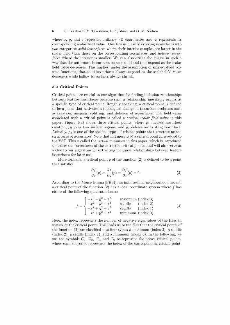
Critical points are crucial to our algorithm for finding inclusion relationshipsbetween feature isosurfaces because such a relationship inevitably occurs ata specific type of critical point. Roughly speaking, a critical point is definedto be a point that activates a topological change in isosurface evolution suchas creation, merging, splitting, and deletion of isosurfaces. The field valueassociated with a critical point is called a critical scalar field value in thispaper. Figure 1(a) shows three critical points, where p1 invokes isosurfacecreation, p2 joins two surface regions, and p3 deletes an existing isosurface.Actually, p2 is one of the specific types of critical points that generate nestedstructures of isosurfaces. Note that in Figure 1(b) a critical point p4 is added tothe VST. This is called the virtual minimum in this paper, which is introducedto assure the correctness of the extracted critical points, and will also serve asa clue to our algorithm for extracting inclusion relationships between featureisosurfaces for later use.
More formally, a critical point p of the function (2) is defined to be a pointthat satisfies
∂f
∂x(p) =
∂f
∂y(p) =
∂f
∂z(p) = 0. (3)
According to the Morse lemma [FK97], an infinitesimal neighborhood arounda critical point of the function (2) has a local coordinate system where f haseither of the following quadratic forms:
f =
⎧⎪⎪⎨⎪⎪⎩
−x2 − y2 − z2 maximum (index 3)−x2 − y2 + z2 saddle (index 2)−x2 + y2 + z2 saddle (index 1)
x2 + y2 + z2 minimum (index 0).
(4)
Here, the index represents the number of negative eigenvalues of the Hessianmatrix at the critical point. This leads us to the fact that the critical points ofthe function (2) are classified into four types: a maximum (index 3), a saddle(index 2), a saddle (index 1), and a minimum (index 0). In the following, weuse the symbols C3, C2, C1, and C0 to represent the above critical points,where each subscript represents the index of the corresponding critical point.

Emphasizing Isosurface Embeddings in Direct Volume Rendering 7
NONEC3
C0
C3
C0
Fig. 2. Isosurface transitions at a maximum and a minimum.
(a)C1
C2 C2
C1
C2
C1
C2
C1
(b)
C2
C1
C2
C1
(c)
(d)C1
C2
C1
C2
Fig. 3. Classification of isosurface transitions at saddles depending on the embed-ding in 3D space. Thick arrows represent transitions of solid isosurfaces while out-lined arrows represent those of hollow isosurfaces. Isosurface inclusion relationshipsoccur only in the transition path (b) (outlined by broken lines).
Figure 2 shows isosurface transitions around a maximum (C3) and a min-imum (C0). At a maximum, a new topological sphere appears in 3D space,while an existing sphere disappears at a minimum.
At a saddle of index 2 (C2) two isosurface regions are merged, while anexisting isosurface region is split into two at a saddle of index 1 (C1). Thus,the corresponding topological changes become more complicated than those atmaxima and minima. Note here that some specific types of saddles definitelyintroduce isosurface inclusion relationships which we are going to emphasize inour rendering process. This requires rigorous classification of isosurface tran-sitions at the saddles by taking into account their embeddings into 3D space.Figure 3 shows such a classification result where each type of saddle possessesfour different topological transitions. Furthermore, the previous assumptionin Section 3.1 restricts such isosurface transitions at saddles as indicated bythick and outlined arrows in the figure. Here, solid isosurfaces can follow onlythe two paths of C2 and the two paths of C1 indicated by the thick arrowsbecause they expand as the scalar field value decreases. On the other hand,hollow isosurfaces follow only the two paths of C2 and two paths of C1 indi-cated by the outlined arrows.
8 S. Takahashi, Y. Takeshima, I. Fujishiro, and G. M. Nielson
We can now derive that an inclusion relationship occurs through only onetransition path shown in Figure 3(b) out of four, for each type of saddle point(i.e. C2 and C1). This enables us to locate inclusion relationships betweenisosurfaces at any scalar field values by identifying transitions at saddles withtheir embeddings. This can be achieved by tracing the links in the VST, whichwill be described later in Section 3.4.
As described previously, our algorithm accounts for the virtual minimum,which is artificially added to the volume function (2) so that we can think of aninput dataset as a topological 3D sphere S3. This setting enables us to checkthe mathematical consistency of the extracted critical points by consultingthe Euler formula [TTF04]:
#{C3} − #{C2} + #{C1} − #{C0} = 0, (5)
where #{Ci} represents the number of critical points of index i.
3.3 Revised Algorithm for VST Construction
For constructing a VST automatically from a given volume dataset, we useour previous algorithm described in [TTF04], which originates from the sur-face analysis framework [TIS+95] used in GIS applications. However, we haveinserted a new step and made some modifications to the existing steps inthe algorithm in order to extract spatial configurations of isosurfaces. Conse-quently, the algorithm has the following five steps:
Step 1: Extract critical points.
This step begins with linear interpolation of the volume dataset through tetra-hedralization, in order to uniquely determine the isosurface evolution as thescalar field value decreases. Here, the tetrahedralization is performed in sucha way that it can simulate the isosurface evolution extracted by using theasymptotic decider [NH91] (See [TTF04] for the details). In the tetrahedral-ization, each voxel has its neighboring voxels that constitute a triangulatedsphere surrounding the target voxel itself. By comparing the scalar field valuesof the neighboring voxels on the sphere with that of the target, the algorithmpartitions the surrounding sphere into two types of connected regions: plusregions that include points having larger scalar field values than the target,and minus regions having smaller scalar field values. By identifying the config-uration of these plus and minus regions on the sphere, we can extract criticalpoints together with their types.
Step 2: Construct a VFN.
Before constructing a VST from the volume dataset, our algorithm constructsa graph called a voxel flow network (VFN) that works as an intermediate rep-resentation in the overall process. Constructing the VFN begins with tracing
Emphasizing Isosurface Embeddings in Direct Volume Rendering 9
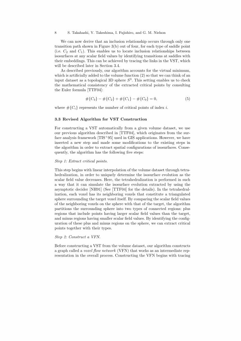
C3 C2 C1 C0
C3 3-C2 2-C2 3-C1 2-C1 C0
Fig. 4. VST parts around critical points.
voxel flows which emanate from each saddle critical point. From each saddle,we traverse voxel flows from its neighbors having the larger (smaller) scalarfield value up to maxima (down to minima) along the steepest ascent (descent)direction. The VFN is then introduced to capture the scalar field configura-tion between the critical points, where its node represents the critical pointand its link represents the voxel flow.
Step 3: Convert the VFN into a VST.
In this step, the constructed VFN is converted to a VST by fixing the linksin the VST from its ends to center. This is possible because the VST is con-structed by assembling the parts as shown in Figure 4 where each part involvesone critical point. Recall that the VST node signifies the critical point andits link represents one isolated interval volume swept by an evolving isosur-face component. Details of the conversion process can be found in [TTF04].Note that the resultant VST becomes a tree because the input volume datasetsatisfies the assumption of single-valued functions. (See Section 3.1.)
Step 4: Mapping between voxels and the VST links.
This step is newly introduced here in order to establish a mapping from eachvoxel onto a VST link, which will help us generate an additional dimension formulti-dimensional transfer functions that emphasize nested inner structuressystematically. The mapping is defined to match a voxel to the link in such away that the interval volume corresponding to the link involves the voxel. Forexample, voxels involved in the interval volumes shaded in dark gray, lightgray, and white in Figure 1(a) are mapped onto the links p1p2 (in dark gray),p2p3 (in light gray), and p2p4 (in white) in Figure 1(b), respectively. In ourimplementation, each voxel has a pointer to its corresponding link while thelink also has a pointer to the voxel.
The algorithm constructs the mapping without explicitly extracting isosur-faces at every scalar field value. We can match the voxel to the correspondinglink by finding its neighboring voxels that have already been mapped to thesame link of the VST in most cases. If this is not the case, we find the localmaximum and minimum reachable from the voxel using the tracing processsimilar to that in Step 2. In addition, we extract candidate links that go acrossthe scalar field value of the current voxel, and trace the VST from each can-didate link constantly with respect to the scalar field to collect a set of end
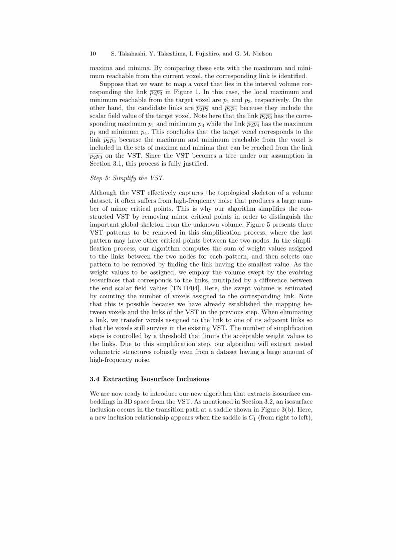
10 S. Takahashi, Y. Takeshima, I. Fujishiro, and G. M. Nielson
maxima and minima. By comparing these sets with the maximum and mini-mum reachable from the current voxel, the corresponding link is identified.
Suppose that we want to map a voxel that lies in the interval volume cor-responding the link p2p3 in Figure 1. In this case, the local maximum andminimum reachable from the target voxel are p1 and p3, respectively. On theother hand, the candidate links are p2p3 and p2p4 because they include thescalar field value of the target voxel. Note here that the link p2p3 has the corre-sponding maximum p1 and minimum p3 while the link p2p4 has the maximump1 and minimum p4. This concludes that the target voxel corresponds to thelink p2p3 because the maximum and minimum reachable from the voxel isincluded in the sets of maxima and minima that can be reached from the linkp2p3 on the VST. Since the VST becomes a tree under our assumption inSection 3.1, this process is fully justified.
Step 5: Simplify the VST.
Although the VST effectively captures the topological skeleton of a volumedataset, it often suffers from high-frequency noise that produces a large num-ber of minor critical points. This is why our algorithm simplifies the con-structed VST by removing minor critical points in order to distinguish theimportant global skeleton from the unknown volume. Figure 5 presents threeVST patterns to be removed in this simplification process, where the lastpattern may have other critical points between the two nodes. In the simpli-fication process, our algorithm computes the sum of weight values assignedto the links between the two nodes for each pattern, and then selects onepattern to be removed by finding the link having the smallest value. As theweight values to be assigned, we employ the volume swept by the evolvingisosurfaces that corresponds to the links, multiplied by a difference betweenthe end scalar field values [TNTF04]. Here, the swept volume is estimatedby counting the number of voxels assigned to the corresponding link. Notethat this is possible because we have already established the mapping be-tween voxels and the links of the VST in the previous step. When eliminatinga link, we transfer voxels assigned to the link to one of its adjacent links sothat the voxels still survive in the existing VST. The number of simplificationsteps is controlled by a threshold that limits the acceptable weight values tothe links. Due to this simplification step, our algorithm will extract nestedvolumetric structures robustly even from a dataset having a large amount ofhigh-frequency noise.
3.4 Extracting Isosurface Inclusions
We are now ready to introduce our new algorithm that extracts isosurface em-beddings in 3D space from the VST. As mentioned in Section 3.2, an isosurfaceinclusion occurs in the transition path at a saddle shown in Figure 3(b). Here,a new inclusion relationship appears when the saddle is C1 (from right to left),

Emphasizing Isosurface Embeddings in Direct Volume Rendering 11
C3–C2: C0–C1: C2–C1:
Fig. 5. VST patterns to be eliminated in the simplification process.
C2 C1
(a1)solid solid
solid(a2)
hollow
hollow hollow
(b1)solidhollow
hollow(b2)
solid
hollowsolid
(c1)hollow
hollow(c2)
solid
solid
(d1)solid
solid(d2)
hollow
hollow
Fig. 6. Isosurface embeddings around saddles: Each row corresponds to the isosur-face transition in Figure 3, and the arrows represents the direction of tracing.
and an existing inclusion relationship dissolves when the saddle is C2 (fromleft to right) when lowering the corresponding scalar field value. This impliesthat, in order to extract the inclusion relationships, we have to identify eachVST part around a saddle point in Figure 4, with a topological transition ofan isosurface in Figure 3.
The assumption made in Section 3.1 restricts topological transitions ofsolid and hollow isosurfaces at saddles as shown in Figure 3. This enablesa one-to-one correspondence between the VST components (Figure 4) andisosurface transitions (Figure 3), once we can identify the incident links withsolid or hollow isosurface components. Figure 6 illustrates VST parts thatcorrespond to the four paths of isosurface transitions in Figure 3 row by rowfor each of C2 and C1, where each link incident to a saddle is recognized as solid(indicated by a think arrow) or hollow (indicated by an outlined arrow). Thisallows us to identify all the links in the VST with solid or hollow isosurfacesby consulting Figure 6.
Our algorithm finds each link in the VST to be solid or hollow, by travers-ing the links in the VST. In practice, this tracing process starts from thevirtual minimum because the link incident to the virtual minimum is known

12 S. Takahashi, Y. Takeshima, I. Fujishiro, and G. M. Nielson
to represent an outermost solid isosurface under the assumption in Section 3.1.Furthermore, the virtual minimum can easily be distinguished from other crit-ical points since it is artificially introduced to the volume dataset.
In our implementation, the virtual minimum serves as a starting point fortracing solid links of the VST in the upward direction, especially to checkhow outermost isosurfaces evolve as the scalar field value increases. Duringthe tracing process, each critical point on the way is identified with a VSTpart in Figure 6 according to the attribute (solid or hollow) of the incominglink, and other unvisited outgoing links are also matched with solid or hollowby consulting the corresponding part in Figure 6. The unvisited links are thenregistered to a queue Qs in the algorithm if they are solid, and registeredto another queue Qh if hollow. Note that these two queues are FIFOs. Afterhaving examined the current critical point, the algorithm removes one solidlink from the queue Qs to process it next. Here, the queue Qs stores unvisitedsolid links that are examined in the ongoing upward tracing process whilethe queue Qh stores hollow links to be handled in the next downward tracingprocess. Consequently, this upward tracing process ends when the queue Qs
becomes empty. After that, we examine the queue Qh and begin the tracingprocess in the opposite (downward) direction for hollow links this time. Theoverall tracing process continues until all the links in the VST are processed.
When identifying a saddle point in the VST with a topological transition,we will encounter the four types of the parts around saddles as shown inFigure 4: 3-C2, 2-C2, 3-C1, and 2-C1. The arrows in Figure 6 show how eachof the four parts is traced in the upward and downward tracing processesdepending on the attributes of its incident links. When tracing solid linksin the upward direction, the four types of parts 3-C2, 2-C2, 3-C1, and 2-C1 in Figure 4 correspond to those in Figures 6(a1), (d1), (b2), and (c2),respectively. On the other hand, these four types are matched to the parts inFigures 6(b1), (c1), (a2), and (d2) when tracing hollow links. Note that a newinclusion relationship only occurs in the part of Figure 6(b2) and an existinginclusion relationship disappears in the part of Figure 6(b1), when reducingthe scalar field value. Figure 1(b) shows how to trace the VST links for theanalytic function (1) with the arrows indicating the tracing directions. In thiscase, the node p2 is identified with the part in Figure 6(b2), which implies theexistence of isosurface inclusion relationships.
Our method stores such inclusion relationships between isosurfaces for eachinterval between two adjacent critical scalar field values because the inclusionrelationships do not change within that interval. In our implementation, weassign a tree data representation to each interval so that the tree can rep-resent inclusion relationships between any pairs of connected components ofan isosurface. Here, the inclusion relationship is represented by the link ofthe tree where its parent and child nodes correspond to the outer and in-ner isosurfaces, respectively. Figure 7 shows such isosurface inclusion trees forthe analytic function (1). Note that each of the trees introduces an artificialroot node (illustrated as outlined circles) because we assume that the virtual

Emphasizing Isosurface Embeddings in Direct Volume Rendering 13
scalar field value
C3
C1
C0
C0
p4
p3
p1
10
2
10
2
10
2
f(p1)
p2 f(p2)
f(p3)
f(p4)inclusionlevel
Fig. 7. VST and its isosurface inclusion trees of the analytic function (1).
isosurface includes all the existing isosurfaces within the interval. This repre-sentation scheme comes from the previous work on designing 3D surfaces byusing their topological skeleton [SKK91, TSK97]. In our framework, this datarepresentation plays an important role in emphasizing nested inner structuresusing multi-dimensional transfer functions.
4 Emphasizing Isosurface Embeddings
While the aforementioned algorithm successfully extracts nested structures offeature isosurfaces, it is still a challenging task to effectively emphasize suchnested structures in the visualization stage because the conventional transferfunctions depend only on the scalar field. This means that the conventionaltransfer functions cannot distinguish between nested isosurfaces if they areat the same scalar field value. Thus, emphasizing inner and outer isosurfacesindividually requires more sophisticated transfer functions that depend onrelative geometric positions in addition to the scalar field.
To this end, we developed a new algorithm that effectively accentuatessuch nested structures using multi-dimensional transfer functions. The con-cept of multi-dimensional transfer functions was originally introduced byLevoy [Lev88], where he employed a 2D opacity transfer function that usesgradient magnitude for the second dimension. In our framework, we also for-mulate a 2D opacity transfer function while we employ a different attributevalue called an inclusion level for the second dimension.
In the remainder of this section, we begin by designing conventional 1Dtransfer functions by referring to the VST. We then define 2D transfer func-tions that accept the inclusion levels as the second dimension in order toemphasize the nested structures of isosurfaces.

14 S. Takahashi, Y. Takeshima, I. Fujishiro, and G. M. Nielson
0 255
hue
scalar field
cm
2π
c1c2c3cm-1
(a)
opacity
0 255scalar fieldr2 r1rm-1
opacity
0 255scalar fieldsolid
solidhollow
hollow
12
rm-1 r2 r1
34
inclusionlevel
(b) (c)
Fig. 8. Transfer function design principles: (a) hue, (b) 1D opacity and (c) 2Dopacity.
4.1 Design Principles of 1D Transfer Functions
Since the VST robustly extracts the global structure of a given volume dataset,it allows us to easily identify feature isosurfaces to be emphasized in thevisualization stage. As the feature isosurfaces, our rendering framework selectssignificant isosurface components from each scalar field interval bound byadjacent critical scalar field values. In practice, we define a representativescalar field value as the midpoint of each scalar field interval and extractthe corresponding isosurface as representative isosurfaces to illuminate thedistinctive isosurface transition in the volume. These representative isosurfaceswill be also suitable for expressing inner structures of the given volume if weconsider the nested structures there.
In our implementation, the scalar field values are mapped affinely onto an8-bit range [0, 255], and c1, c2, . . . , cm represent a sequence of critical scalarfield values in descending order, where cm is the scalar field value of thevirtual minimum and set to be 0. Although there may be multiple candidatesfor design principles of 1D transfer functions, we use the hue and opacitytransfer functions shown in Figures 8(a) and (b) as the common principles.
The hue transfer function maps the scalar field onto the range [0, 2π] onthe top of the HSV hexcone. Furthermore, in our design principle, each scalarfield interval [ci+1, ci] (i = 1, . . . , m− 1) has a hue range of the same interval,and it has linear descent slope of the hue value as shown in Figure 8(a). Notethat the hue transfer function is 1D and depends only on the scalar field value
Emphasizing Isosurface Embeddings in Direct Volume Rendering 15
255
250
246
representativeisosurface
scalarfield value
p1
p2
p3
p4
virtual minimum
VST
253
248
123
representativefield value
r1
r2
r3
0(=c4)
c1
c2
c3
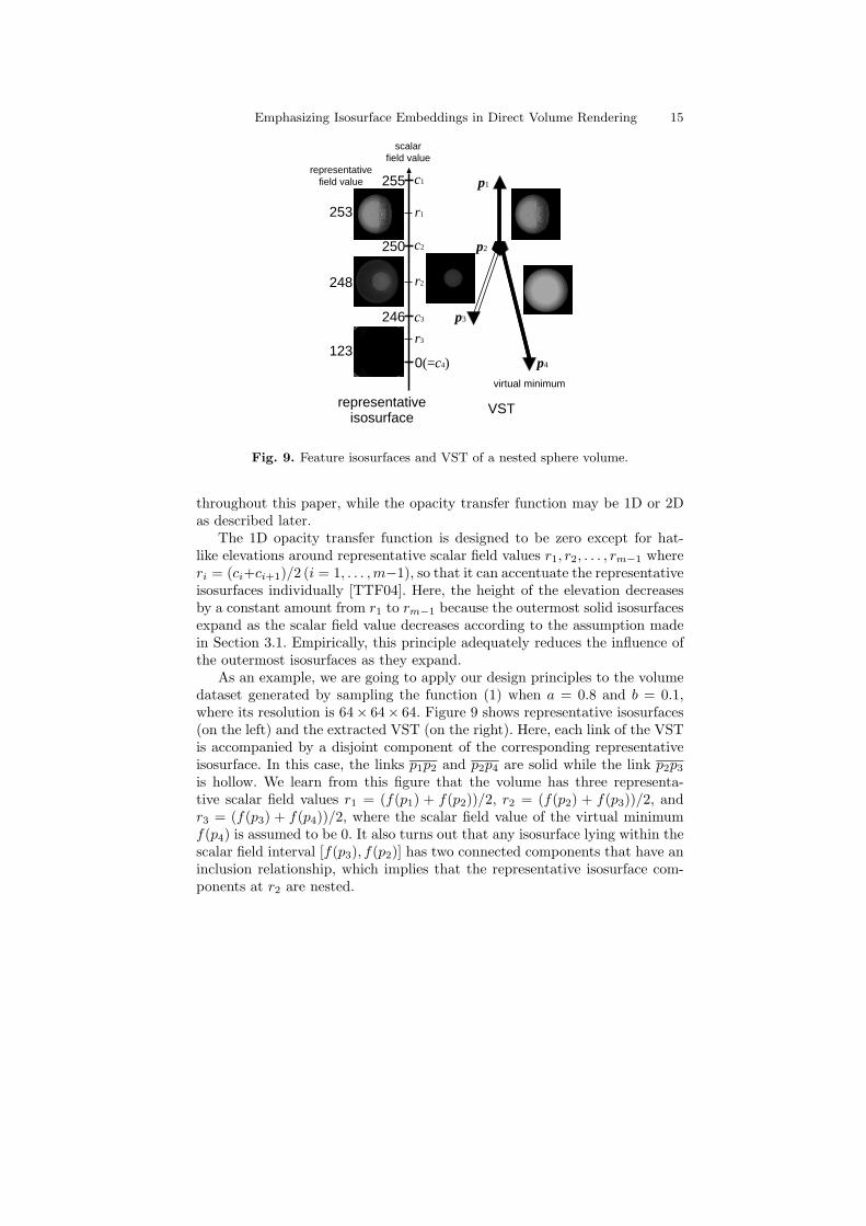
Fig. 9. Feature isosurfaces and VST of a nested sphere volume.
throughout this paper, while the opacity transfer function may be 1D or 2Das described later.
The 1D opacity transfer function is designed to be zero except for hat-like elevations around representative scalar field values r1, r2, . . . , rm−1 whereri = (ci+ci+1)/2 (i = 1, . . . ,m−1), so that it can accentuate the representativeisosurfaces individually [TTF04]. Here, the height of the elevation decreasesby a constant amount from r1 to rm−1 because the outermost solid isosurfacesexpand as the scalar field value decreases according to the assumption madein Section 3.1. Empirically, this principle adequately reduces the influence ofthe outermost isosurfaces as they expand.
As an example, we are going to apply our design principles to the volumedataset generated by sampling the function (1) when a = 0.8 and b = 0.1,where its resolution is 64× 64× 64. Figure 9 shows representative isosurfaces(on the left) and the extracted VST (on the right). Here, each link of the VSTis accompanied by a disjoint component of the corresponding representativeisosurface. In this case, the links p1p2 and p2p4 are solid while the link p2p3
is hollow. We learn from this figure that the volume has three representa-tive scalar field values r1 = (f(p1) + f(p2))/2, r2 = (f(p2) + f(p3))/2, andr3 = (f(p3) + f(p4))/2, where the scalar field value of the virtual minimumf(p4) is assumed to be 0. It also turns out that any isosurface lying within thescalar field interval [f(p3), f(p2)] has two connected components that have aninclusion relationship, which implies that the representative isosurface com-ponents at r2 are nested.

16 S. Takahashi, Y. Takeshima, I. Fujishiro, and G. M. Nielson
Figure 10(a) shows a visualization result of this dataset obtained by usingthe 1D transfer functions in Figures 8(a) and (b). Although the result seemsto be effective, it still obscures the isosurface inclusion at the representativescalar field value r2. This motivates us to incorporate an additional attributefor the multi-dimensional transfer functions as described below.
4.2 Design Principles of 2D Transfer Functions
An inclusion level is the second variable for our multi-dimensional transferfunctions, and represents the depth of the corresponding isosurface compo-nent in a nested tree structure as shown in Figure 7. Thus, it allows us tosystematically locate the relative geometric position of each voxel within sucha nested volumetric structure. Moreover, the inclusion level also differs fromthe conventional attributes for multi-dimensional transfer functions in that itis a topological attribute and comes from the rigorous analysis of the globalvolumetric structures, while all the conventional attributes represent localvolumetric properties such as derivatives [KD98] and curvatures [HKG00].
Actually, our algorithm will calculate this attribute value for each voxel byconsulting the data structure as shown in Figure 7. Here, the VST togetherwith its associated trees for isosurface inclusions is embedded into 3D space. Inthe figure, the vertical and depth axes represent the scalar field and inclusionlevel, respectively, and the lateral lines on each horizontal plane represent thescales of the inclusion level for each isosurface inclusion tree.
Since we have already established the mapping between the voxels and theVST links in Section 3.3, we can easily calculate the inclusion levels for allthe voxels by handling the VST links one by one. Suppose we are now lookingat the link p2p4 in Figure 9. From the mapping, our algorithm retrieves thearray of voxels that belong to the link. Each voxel is then distributed tothe corresponding scalar field interval according to its scalar field value. Forexample, in this case, if the voxel has a larger scalar field value than p3, it willbe assigned to the interval [f(p3), f(p2)]. Otherwise, it will be delivered to theinterval [f(p4), f(p3)]. The inclusion level can be obtained by evaluating thedepth of its VST link in the corresponding isosurface inclusion tree, becausethe tree represents isosurface spatial configurations within the scalar fieldinterval to which the voxel is distributed.
It should be noted that the inclusion level is intrinsically discrete and mayhave gaps at some critical scalar field values because the inclusion relationshipsbetween isosurface components suddenly change at the values. These gapscould result in unexpected artifacts in our final visualization results. We thusavoid these artifacts by linearly interpolating the gap so that the inclusion levelbecomes continuous. Figure 7 shows such an example, where the inclusionlevel of the link p2p3 linearly rises from 1 to 2 while the scalar field valuereduces from f(p2) to (f(p2) + f(p3))/2. In practice, our algorithm assignsthe intermediate inclusion levels to the voxels according to their scalar fieldvalues.

Emphasizing Isosurface Embeddings in Direct Volume Rendering 17
Now we are ready to extend the previous 1D opacity transfer function to2D so that it effectively emphasizes the nested isosurfaces with the help of theinclusion levels. As described previously, the height of the hat-like elevationfor the 1D opacity transfer function reduces by a constant amount at eachrepresentative scalar field value as the scalar field value decreases as shown inFigure 8(b). This is because solid isosurfaces expand while the correspondingscalar field value decreases as described in Section 3.1. However, hollow iso-surfaces have the reverse behavior, i.e., they shrink as the scalar field valuedecreases. This lets us raise the height of hat-like elevation for hollow isosur-faces to clarify their topological changes in deeper positions.
By taking these points into account, we design the 2D opacity transferfunction as shown in Figure 8(c). Here, at each discrete inclusion level, the hat-like elevation decreases if the corresponding isosurface is solid and increasesif hollow as the scalar field value goes down. We then define the opacity forintermediate non-integer inclusion levels by interpolating between those oninteger inclusion levels. This means that the opacity transfer function aroundthe representative scalar field values has a form of hyperbolic paraboloid. Notethat the opacity transfer function is defined to increase as the inclusion levelbecomes larger. This is achieved by ensuring that the maximum opacity valueat the inclusion level l does not exceed the minimum opacity of the inclusionlevel l + 1.
Our experiments show that this design principle makes the inner isosur-face components clearly visible through the outer ones, and avoids obscuringthe nested inner structures. Figure 10(b) shows such an example where thenested structure of the isosurface components at (f(p2) + f(p3))/2 is effec-tively emphasized. The previous 1D color transfer function is used for thesevisualization results.
5 Application to Real Datasets
In this section, we apply the present framework to two datasets in order todemonstrate its applicability to real datasets. In all of these datasets, thescalar field values were normalized to an 8-bit range [0, 255]. In our experi-ments, the present algorithms are implemented on an ordinary PC environ-ment (CPU: Pentium IV, 2.4GHz, RAM: 1GB).
5.1 Nucleon
The first example is a “nucleon” dataset presented in Figure 11. This datasetis obtained by simulating two-body distribution probability of a nucleon inthe atomic nucleus 16O [Mei], and its resolution here is 41 × 41 × 41. Fromthe dataset, our algorithm extracted a VST as shown in Figure 11(a), whichshows that the dataset actually involves isosurface inclusions within the scalar

18 S. Takahashi, Y. Takeshima, I. Fujishiro, and G. M. Nielson
(a) (b)
Fig. 10. Emphasizing isosurface embeddings of a nested sphere volume: (a) with1D transfer functions, and (b) with 2D transfer functions.
247
scalar field
249
193189187161103130
virtual minimum
p1
p2
p3
p4
p5
p6
p7
p8p9
(a) (b) (c)
(d) (e)
Fig. 11. Inner structure of the “nucleon” dataset [Mei]: (a) The VST. Visualizationresults (b) with naive (linear hue and flat opacity) 1D transfer functions, (c) withtopologically-accentuated 1D transfer functions, (d) with 2D transfer functions, and(e) generated using emission-only optical model.
198132
118
98
5
virtual minimum
123128
112
38
scalar field
p1
p3
p2
p5
p4
p6
p8
p7
p9p10
(a) (b) (c)
Fig. 12. Antiproton-hydrogen atom collision volume dataset: (a) the VST. Visual-ization results (b) with 1D transfer functions, and (c) with 2D transfer functions.

Emphasizing Isosurface Embeddings in Direct Volume Rendering 19
field interval [0, 161]. Note that a link for a solid isosurface is in blue whilethat for a hollow isosurface is in orange in this figure.
As described in Section 1, Figure 11(b) obscures the inner structures andprovides no useful information because it is generated using naive transferfunctions. While Figure 11(c) accentuates representative isosurfaces individu-ally using the conventional 1D transfer functions [FATT00, WSHH02, TTF04],it still misses the nested inner structures which we are interested in, unfor-tunately. On the other hand, Figure 11(d) effectively emphasizes the innerisosurface components due to the use of 2D transfer functions with the inclu-sion levels.
5.2 Antiproton-Hydrogen Atom Collision
As the second example, we consider the antiproton-hydrogen atom collisionat intermediate collision energy below 50keV. In the antiproton-hydrogen col-lision system, a single antiproton comes into collision with a single hydrogenatom. The details of the formulation and established numerical schemes canbe found in [SSK02].
Here, we applied our framework to the dataset with a resolution of64× 64× 64. Figure 12(a) shows the VST extracted from this dataset. Whenexploring isosurface transitions as the scalar field value reduces, we can seethat the isosurface component of the link p2p5 splits into nested isosurfacecomponents of the links p5p7 and p5p10 at the scalar field value 118, and si-multaneously encloses another isosurface component of the link p4p6. Afterthat, the enclosed isosurface of the link p4p6 also divides itself into the nestedsurface components of the links p6p7 and p6p8 at 112. This means that wehave fourfold nested structures in the scalar field interval [98, 112].
Figures 12(b) and (c) show rendered images of the antiproton-hydrogenatom collision volume dataset. Figure 12(b) shows a rendered image gener-ated using the conventional 1D transfer functions, where representative iso-surfaces are accentuated while ignoring their accompanying nested structures.As shown in the figure, the nested structure lying in the scalar field interval[98, 112] was densely occluded by the outermost isosurface component. Onthe other hand, our new algorithm clearly emphasizes the nested structuresas shown in Figure 12(c) where 2D opacity transfer function is applied. Notehere that our algorithm controls voxel opacities by taking into account isosur-face embeddings using the multi-dimensional transfer functions. These resultssuggest that our present framework can explicitly extract significant volumet-ric structures that may be missed by using the conventional methods.
6 Discussion
This section discusses the validity of the present framework for emphasizingisosurface embeddings in direct volume rendering.

20 S. Takahashi, Y. Takeshima, I. Fujishiro, and G. M. Nielson
6.1 Comparison with an Emission-Only Optical Model
The present framework effectively emphasizes isosurface embeddings in vol-ume rendering because it can extract inclusion relationships between isosur-faces by tracing their global transitions in a given volume. On the other hand,another promising approach may be an emission-only optical model where allthe feature isosurface components equally contribute to the final image andnone is attenuated by the surrounding components. Figure 11(e) is an imagegenerated by using this model. However, when compared with Figure 11(d)that is generated by our new framework, this model cannot suppress the opac-ity of outer isosurfaces while emphasizing inner ones because it lacks the abil-ity to distinguish between outer and inner isosurfaces. This shows that thepresent framework provides more sophisticated visualization techniques thanthe simple emission-only optical model.
6.2 Computational Cost
The computational cost is another issue to be considered since the presentframework requires more computational time for the rigorous analysis of agiven volume. In practice, our algorithm extracted nested isosurface struc-tures in 4 minutes for the “nucleon” dataset (Figure 11(d)) and 30 minutesfor the antiproton-hydrogen atom collision dataset (Figure 12(c)). However,these computational costs can be reduced remarkably by introducing adap-tive tetrahedralization for the interpolation of the given scalar field withoutsacrificing the accuracy of the analysis [TNTF04]. According to the resultsin [TNTF04], it took only 25 seconds for the “nucleon” dataset, and 60 sec-onds even for the high-resolution version (129× 129× 129) of the antiproton-hydrogen atom collision dataset. This concludes that the present frameworkwill be a more promising approach for comprehensible volume rendering asthe computational performance becomes better in future.
7 Conclusion
This paper has presented a new rendering framework that clearly emphasizesnested isosurface structures embedded in the given volume datasets. The keyto the present framework is the use of multi-dimensional transfer functionsthat assign different optical properties to each voxel. This is achieved by usingthe inclusion level as well as the conventional scalar field. In order to calcu-late such an additional attribute, we developed a new algorithm that extractsinclusion relationships between feature isosurfaces by tracing the topologi-cal skeleton delineated from the given dataset. Several experimental resultsdemonstrated the feasibility of the present method.
As a future research theme, we plan to take into account psychologicalfactors of color science so that we can accommodate the inclusion level as

Emphasizing Isosurface Embeddings in Direct Volume Rendering 21
a new dimension when designing color transfer functions. Furthermore, ourframework may also provide the basis for future research on incorporating tex-tures and lighting properties because such properties may provide significantlandmarks on the visualization results.
Acknowledgements
We wish to acknowledge the support of the Japan Society of the Promotionof Science under Grants-in-Aid for Young Scientists (B) (No. 14780189), theOkawa Foundation for Information and Telecommunications, the Office ofNaval Research (N00014-02-1-0287), the National Science Foundation (NSFIIS-9980166 & ACI-0083609), and DARPA (MDA972-00-1-0027).
References
[BPS97] C. L. Bajaj, V. Pascucci, and D. R. Schikore. The contour spectrum.In Proc. of IEEE Visualzation ’97, pages 167–173, 1997.
[CKLG98] S. Castro, A. Konig, H. Loffelmann, and E. Groller. Trans-fer function specification for the visualization of medical data.Technical Report TR–186–2–98–12, Vienna University of Technol-ogy, 1998. [http://www.cg.tuwien.ac.at/research/TR/98/TR-186-2-98-12Abstract.html].
[CMH+01] B. Csebfalvi, L. Mroz, H. Hauser, A. Konig, and E. Groller. Fast vi-sualization of object contours by non-photorealistic volume rendering.Computer Graphics Forum, 20(3):452–460, 2001.
[COCSD00] D. Cohen-Or, Y. Chrysanthou, C. Silva, and G. Drettakis. Visibility,problems, techniques and applications. Siggraph ’00 Course Notes,2000.
[CSA03] H. Carr, J. Snoeyink, and U. Axen. Computing contour trees in alldimensions. Computational Geometry, 24(2):75–94, 2003.
[FAT99] I. Fujishiro, T. Azuma, and Y. Takeshima. Automating transfer func-tion design for comprehensive rendering based on 3D field topologyanalysis. In Proc. of IEEE Visualization ’99, pages 467–470, 563, 1999.
[FATT00] I. Fujishiro, T. Azuma, Y. Takeshima, and S. Takahashi. Volume datamining using 3D field topology analysis. IEEE Computer Graphics &Applications, 20(5):46–51, 2000.
[FK97] A. T. Fomenko and T. L. Kunii. Topological Modeling for Visualization,chapter 6, pages 105–125. Springer-Verlag, 1997.
[FMS95] I. Fujishiro, Y. Maeda, and H. Sato. Interval volume: A solid fittingtechnique for volumetric data display and analysis. In Proc. of IEEEVisualization ’95, pages 151–158, CP–18, 1995.
[FMST96] I. Fujishiro, Y. Maeda, H. Sato, and Y. Takeshima. Volumetric dataexploration using interval volume. IEEE Transactions on Visualizationand Computer Graphics, 2(2):144–155, 1996.
[FTTY02] I. Fujishiro, Y. Takeshima, S. Takahashi, and Y. Yamaguchi.Topologically-accentuated volume rendering. In F. H. Post, G. M.Nielson, and G.-P. Bonneau, editors, Data Visualization: The State ofthe Art, pages 95–108. Kluwer Academic Publishes, 2002.

22 S. Takahashi, Y. Takeshima, I. Fujishiro, and G. M. Nielson
[HKG00] J. Hladuvka, A. Konig, and E. Groller. Curvature-based transfer func-tions for direct volume rendering. In Proc. of Spring Conference onComputer Graphics 2000, pages 58–65, 2000.
[Int97] V. L. Interrante. Illustrating surface shape in volume data via principaldirection-driven 3D line integral convolution. In Computer Graphics(Proc. of Siggraph ’97), pages 109–116, 1997.
[KD98] G. Kindlmann and J. W. Durkin. Semi-automatic generation of trans-fer functions for direct volume rendering. In Proc. of IEEE Symposiumon Volume Visualization, pages 79–86, 1998.
[KKH01] J. Kniss, G. Kindlmann, and C. Hansen. Interactive volume render-ing using multi-dimensional transfer functions and direct manipulationwidgets. In Proc. of IEEE Visualization 2001, pages 255–262, 2001.
[KKH02] J. Kniss, G. Kindlmann, and C. Hansen. Multidimensional transferfunctions for interactive volume rendering. IEEE Transactions on Vi-sualization and Computer Graphics, 8(3):270–285, 2002.
[KS00] J. T. Klosowski and C. T. Silva. The prioritized-layered projection al-gorithm for visible set estimation. IEEE Transactions on Visualizationand Computer Graphics, 6(2):108–123, 2000.
[Lev88] M. Levoy. Display of surfaces form volume data. IEEE ComputerGraphics & Applications, 8(5):29–27, 1988.
[LME+02] A. Lu, C. J. Morris, D. S. Ebert, P. Rheingans, and C. Hansen. Non-photorealistic volume rendering using stippling techniques. In Proc. ofIEEE Visualization 2002, pages 211–218, 2002.
[Mei] M. Meißner. Web Page [http://www.volvis.org/].[NH91] G. M. Nielson and B. Hamann. The asymptotic decider: Removing
the ambiguity in marching cubes. In Proc. of IEEE Visualization ’91,pages 83–91, 1991.
[PCM02] V. Pascucci and K. Cole-McLaughlin. Efficient computation of thetopology of level sets. In Proc. of IEEE Visualization 2002, pages187–194, 2002.
[RE01] P. Rheingans and D. Ebert. Volume illustration: Nonphotorealisticrendering of volume models. IEEE Transactions on Visualization andComputer Graphics, 7(3):253–264, 2001.
[SDDS00] G. Schaufler, J. Dorsey, X. Decoret, and F. X. Sillion. Conservativevolumetric visibility with occluder fusion. In Computer Graphics (Proc.of Siggraph ’00), pages 229–238, 2000.
[SKK91] Y. Shinagawa, Y. L. Kergosien, and T. L. Kunii. Surface coding basedon morse theory. IEEE Computer Graphics & Applications, 11(5):66–78, 1991.
[SSK02] R. Suzuki, H. Sato, and M. Kimura. Antiproton-Hydrogen atom col-lision at intermediate energy. IEEE Computing in Science and Engi-neering, 4(6):24–33, 2002.
[TC00] S. Treavett and M. Chen. Pen-and-ink rendering in volume visualiza-tion. In Proc. of IEEE Visualization 2000, pages 203–210, 2000.
[TIS+95] S. Takahashi, T. Ikeda, Y. Shinagawa, T. L. Kunii, and M. Ueda. Al-gorithms for extracting correct critical points and constructing topo-logical graphs from discrete geographical elevation data. ComputerGraphics Forum, 14(3):181–192, 1995.

Emphasizing Isosurface Embeddings in Direct Volume Rendering 23
[TNTF04] S. Takahashi, G. M. Nielson, Y. Takeshima, and I. Fujishiro. Topolog-ical volume skeletonization using adaptive tetrahedralization. In Proc.of Geometric Modeling and Processing 2004, pages 227–236, 2004.
[TSK97] S. Takahashi, Y. Shinagawa, and T. L. Kunii. A feature-based approachfor smooth surfaces. In Proc. of the ACM 4th Symposium on SolidModeling and Applications, pages 97–110, 1997.
[TTF04] S. Takahashi, Y. Takeshima, and I. Fujishiro. Topological volume skele-tonization and its application to transfer function design. GraphicalModels, 66(1):24–49, 2004.
[vKvOB+97] M. van Kreveld, R. van Oostrum, C. Bajaj, V. Pascucci, andD. Schikore. Contour trees and small seed sets for isosurface traversal.In Proc. of the 13th ACM Symposium on Computational Geometry,pages 212–220, 1997.
[WSHH02] G. H. Weber, G. Scheuermann, H. Hagen, and B. Hamann. Exploringscalar fields using critical isovalues. In Proc. of IEEE Visualization2002, pages 171–178, 2002.
Copyright © 2022 FDOKUMEN


![[Peritoneal pseudomyxoma: An overview emphasizing pathological assessment and therapeutic strategies].](https://static.fdokumen.com/doc/165x107/6331d121b6829c19b80bab58/peritoneal-pseudomyxoma-an-overview-emphasizing-pathological-assessment-and-therapeutic.jpg)