STONY BROOK

UNIVERSITY

Iso-Surface Rendering

2

• A closed surface separates ‘outside’ from ‘inside’ (Jordan theorem)

• In iso-surface rendering we say that all voxels with values > some threshold are ‘inside’,

and the others are ‘outside’

• The boundary between ‘outside’ and ‘inside’ is the iso-surface

• All voxels near the iso-surface have a value close to the iso-threshold or iso-value

• Example:

STONY BROOK

UNIVERSITY

Iso-Surface Rendering

3

• To render an iso-surface we cast the rays as usual...

• But we stop once we have interpolated a value iso-threshold

• The easiest way to select the iso-surface is with the transfer function for α

• We would like to illuminate (shade) the iso-surface based on its orientation to the

light source

• Recall that we need a normal vector for shading

• The normal vector N is the local gradient, normalized

STONY BROOK

UNIVERSITY

Iso-Surfacing Example

4

Foot of the Visible Woman

STONY BROOK

UNIVERSITY5

Different Iso-Levels

• Same data-sets, different

extracted iso-surfaces

• Note that like all surfaces, the

interior of the foot is “empty”

STONY BROOK

UNIVERSITY6

Surface Rendering with Polygons

• We have looked at several direct rendering algorithms for volume

visualization

• Process volume itself with no conversion to other formats

• Speed and efficiency issues for software-based ray-casting

• Much of splatting can be implemented with commodity hardware

• Modern graphics hardware is all triangle-based since much of

computer graphics is still surface-only

• Most applications require only surface rendering

• Today we will see algorithms for exploiting triangle-rendering

hardware for volume visualization

STONY BROOK

UNIVERSITY7

Motivations for Iso-surface Polygonization

• Take advantage of surface graphics techniques

• Exploit inexpensive, yet powerful graphics hardware

• Use OpenGL (DirectX, etc.) to specify shading parameters

• Incorporate polygonized surfaces into other polygon-based software

systems easily

• Familiar object representation format used widely across graphics

and visualization

• Use object-order polygon mesh projection algorithms for rendering

(described next)

STONY BROOK

UNIVERSITY8

Polygon Mesh Definitions

• Rule: if all edge vectors in a face are

ordered counterclockwise, then the

face normal vectors will always point

towards the outside of the object.

• This enables quick removal of back-

faces (back-faces are the faces hidden

from the viewer):

back-face condition: vp • n > 0

STONY BROOK

UNIVERSITY9

Polygon Mesh Data Structure

• Vertex list (v1, v2, v3, v4, ...):

– (x1, y1, z1), (x2, y2, z2), (x3, y3, z3), (x4, y4, z4), ....

• Edge list (e1, e2, e3, e4, e5, ...):

– (v1, v2), (v2, v3), (v3, v1), (v1, v4), (v4, v2), ...

• Face list (f1, f2, ...):

– (e1, e2, e3), (e4, e5, -e1), ... or

– (v1, v2, v3), (v1, v4, v2), ...

• Normal list (n1, n2, ...), one per face or per vertex

– (n1x, n1y, n1z), (n2x, n2y, n2z), ...

• Use pointers or indices into vertex and edge list arrays, when appropriate

• Winged-edge / quad-edge / half-edge data structures

STONY BROOK

UNIVERSITY10

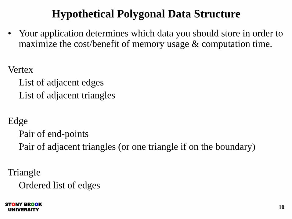
Hypothetical Polygonal Data Structure

• Your application determines which data you should store in order to maximize the cost/benefit of memory usage & computation time.

Vertex

List of adjacent edges

List of adjacent triangles

Edge

Pair of end-points

Pair of adjacent triangles (or one triangle if on the boundary)

Triangle

Ordered list of edges

STONY BROOK

UNIVERSITY11

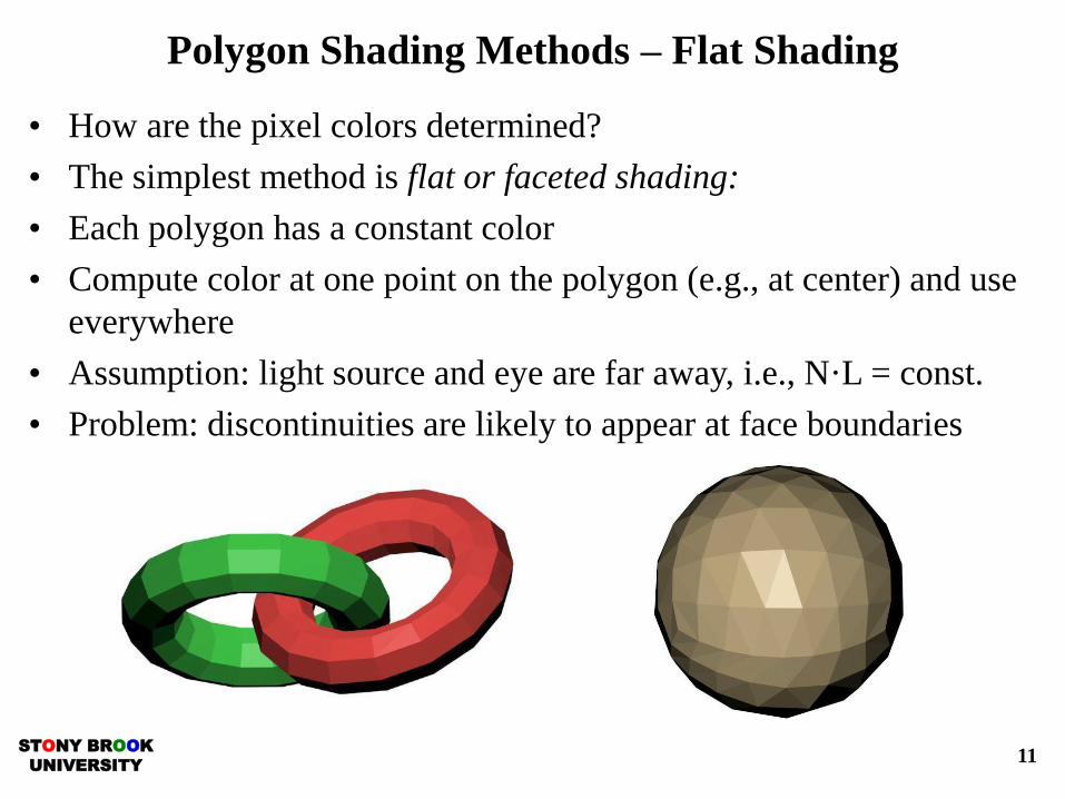
Polygon Shading Methods – Flat Shading

• How are the pixel colors determined?

• The simplest method is flat or faceted shading:

• Each polygon has a constant color

• Compute color at one point on the polygon (e.g., at center) and use

everywhere

• Assumption: light source and eye are far away, i.e., N·L = const.

• Problem: discontinuities are likely to appear at face boundaries

STONY BROOK

UNIVERSITY12

Polygon Shading Methods – Gouraud Shading

• Colors are averaged across polygons along common edges → no more

discontinuities

• Steps:

1. Determine average unit normal at each poly vertex:

2. n: number of faces that have vertex v in common

3. Apply illumination model at each poly vertex → Cv

4. Linearly interpolate vertex colors across edges

5. Linearly interpolate edge colors across scan lines

• Downside: may miss specular highlights at off-vertex

positions or distort specular highlights

STONY BROOK

UNIVERSITY13

Polygon Shading Methods – Phong Shading

• Phong shading linearly interpolates normal vectors, not colors → more realistic

specular highlights

• Steps:

1. Determine average normal at each vertex

2. Linearly interpolate normals across edges

3. Linearly interpolate normals across scanlines

4. Apply illumination model at each pixel to calculate pixel color

• Downside: need more calculations since need to do illumination model at each

pixel

STONY BROOK

UNIVERSITY14

Rendering Polygonal Objects – Hidden Surface Removal

• We have removed all faces that are definitely hidden: the back-faces

• But even the surviving faces are only potentially visible

• They may be obscured by faces closer to the viewer

• Face A of object 1 is partially

obscured by face B of object 2

• Problem of identifying those face

portions that are visible is called

the hidden surface problem

• Solutions:

– Pre-ordering of the faces and subdivision into their visible parts

before display (expensive)

– The z-buffer algorithm (cheap, fast, implementable in hardware)

STONY BROOK

UNIVERSITY15

Overview and Motivation

• Algorithms extract surface of constant density (iso-surfaces) from

3D data and convert it into polygonal mesh

• Divide-and-conquer algorithm

• Process each row of voxels to build the triangulated surface in an

incremental fashion

• Use table to decide on a case-by-case basis how each cell (group of

8 voxels) is used to generate triangles

• Normalized gradient will provide normal direction for the triangles

so we can shade the surface

• Marching Cubes algorithm – developed in 1987, still very widely

used

• Several enhancements since then, but fundamental algorithm

remains the same

STONY BROOK

UNIVERSITY16

The Marching Cubes Polygonization Algorithm

• The Marching Cubes (MC) algorithm converts a volume into a polygonal model

• Allows us to render the iso-surfaces quickly and shade them using flat, Gouraud

or Phong shading (or others)

• Steps:

• Imagine all voxels above the iso-value are set to 1, all others are set to 0

• The goal is to find a polygonal surface that includes all 1-voxels and excludes all

0-voxels

• Look at one volume cell (a cube) at a time → hence the term Marching Cubes

• Here are 2 of ___ possible configurations:

STONY BROOK

UNIVERSITY17

Marching Cubes

• One can identify 15 base cases and use

symmetry and reverses to get the other 241

cases

• The exact position of the polygon vertex on a

cube edge is found by linear interpolation:

• Now interpolate the vertex color by:

c1 = uc2 + (1 – u)c1

• Interpolate the vertex normal by:

n1 = ug2 + (1 – u)g1

g1 and g2 are the gradient vectors at v1 and v2

obtained by central differencing

21

121 )1(

vv

isovuuvuviso

STONY BROOK

UNIVERSITY18

Marching Cubes –Ambiguous Cases

• 2D: ambiguous case:

• 3D: what happens when cases are arbitrarily chosen:

• Remedy: add 6 alternative cases for

3, 6, 7, 10, 12, 13 to prevent holes

STONY BROOK

UNIVERSITY19

Problem with Marching Cubes

• Sharp features, like corners and hard edges, tend to be smoothed

away by the Marching Cubes algorithm

• Finite grid → some details will be lost

• Continuous model discretized onto grid and Marching Cubes

applied:

STONY BROOK

UNIVERSITY20

Model Conversion

• Suppose we wish to represent (convert) a surface model on a

volumetric raster (grid)

• Possible motivation: sculpting operations to modify the object

• This means we need to discretize the 3D geometric shape

• After we have finished our work, we need to convert the 3D

volume back to a surface model

• This can be done with Marching Cubes

• However, at what grid resolution do we store the shape?

• Certain features of the

surface will always be lost

by the regular MC

algorithm

STONY BROOK

UNIVERSITY21

Cause of the Problem

• When we discretize the object, at each voxel we store a distance of

the voxel from the object surface

• Hence, the volume is what we call a volumetric distance field that

approximates a smooth, continuous distance function

• Consider two neighboring grid

points (green) in the vicinity of

a sharp feature (corner) of the

contour S (red)

• Sampling the scalar valued distance function f at both grid points

(blue) and estimating the sample point by linear interpolation leads

to a bad estimation (black) of the true intersection point between the

red contour and the green cell edge

STONY BROOK

UNIVERSITY22

How About Storing a Directed Distance?

• Suppose instead of just storing a scalar value at each voxel, we

store a vector that indicates the directed distance?

• This is still not enough and we replace sharp corners and other

features with diagonal lines

STONY BROOK

UNIVERSITY23

Scalar Distances vs. Directed Distances

• First image: original model

• Second image: discretized and MC applied to a scalar distance field

• Third image: discretized and MC applied to directed distance field

STONY BROOK

UNIVERSITY24

Solution to Loss of Features Problem

• The solution to this problem involves use more information inferred by the data

• During discretization, we compute and store tangent vectors that we compute

using the surface normal

• These vectors basically tell you in what the direction(s) the surface is moving

• Then, when we are left with only the discrete grid, we extend these tangents into

the center of the cells to approximate the character of the surface inside the cell

• Where these tangents intersect, we create a feature point we use to polygonize the

surface

• Blue: original contour we discretized

• Red: extended tangents

• Vertex: feature point we will use

to build polygons

• Black: what directed distances would

have given us

STONY BROOK

UNIVERSITY25

Extended Marching Cubes

• Algorithm:

• If cell contains a sharp feature, determine if an edge feature (green)

or a corner feature (red) is present

• If yes, apply the new technique for selecting vertex positions

• Otherwise, apply the normal Marching Cubes algorithm

STONY BROOK

UNIVERSITY26

Application – Remeshing

• Remeshing of a polygonal mesh

• Generally speaking, skinny or sliver

triangles are bad

• Poor rendering quality

• Interfere with mechanical simulation

• Often too many triangles present to

represent the given object: wastes

computation time, memory, storage

space, etc.

• Extended MC algorithm takes

discretized version of original mesh

and extracts a new surface that has

fewer triangles and also higher

quality triangles

STONY BROOK

UNIVERSITY27

Application – CSG

• Constructive Solid Geometry (CSG) is a shape design technique

• Objects defined as the addition and subtraction of other objects

• Typically difficult to achieve accurately over a discrete grid

• Usually we have to compute intersections between design primitives exactly

(spheres, cylinders, boxes, splines, etc.)

• Very expensive process that involves root-finding

• In discrete grid, problem much simpler by

performing set inclusion/exclusion tests

• The extended Marching Cubes algorithms

makes CSG feasible on a discrete grid

because we can recover these intersected

regions almost exactly

STONY BROOK

UNIVERSITY28

Marching Tetrahedra

• Another iso-surface extraction algorithm is

called Marching Tetrahedra

• Divide each cell into five tetrahedra

• Apply one of the three unique cases

• No ambiguity problem, as with Marching

Cubes

• Easier to implement

• But surface quality is usually not as good

since less information is taken into

consideration (four values used for

interpolation instead of eight)

• Also generates more triangles than MC, the

latter of which might be able to generate a

single large triangle instead of several small

ones to cover the same surface area

STONY BROOK

UNIVERSITY29

Use Volume Rendering to Handle Iso-surfaces

• We saw earlier how we can use ray-casting to

render iso-surfaces by using an alpha transfer

function with a sharp drop-off

• Suppose we don’t have a ray-casting system

available?

• We can instead use an iso-surface extraction

algorithm to generate a polygonal

approximation of the iso-surface implied by the

volumetric data

• Pre-processing step, possibly slow

• User specifies the designed iso-level, and the

algorithm produces the corresponding

triangular iso-surface

STONY BROOK

UNIVERSITY

Gradient Modulation

30

• One use of the gradient is in a process known as gradient modulation in which we modulate the opacity/color of a voxel by the gradient

• First we look up the voxel’s opacity/color, given by the transfer function

• Then we multiply the opacity and color by some function of the gradient magnitude (also given by a transfer function, #5)

• Regions of high gradient magnitude cause an increase in opacity, whereas regions of low gradient magnitude cause the opacity to drop to near zero

• Remind us: what does a high magnitude signify?

• How does this explain the image on the right?

STONY BROOK

UNIVERSITY

Iso-Surface Shading

31

• The normal vector is the normalized

gradient vector g

• N = g / |g| (normal vector always has unit

length)

• Once the normal vector has been

calculated we shade the iso-surface at the

sample point

• The color so obtained is then written to

the pixel that is due to the ray

• Colors are computed using one of the

standard illlumination models

• Let’s see a short movie to see this in

practice (9)

STONY BROOK

UNIVERSITY

Iso-Surface Rendering –Algorithm (Perspective)

32

RenderIsoSurface(Volume V, int stepSize)

for each image pixel p(i, j)

ray = (p(i, j) - eye) / | (p(i, j) - eye) |; // the ray direction vector, normalized

t = 0; // start at the eye point

do forever

sampleLoc = eye + t · stepSize · ray // step along the ray

intVal = Interpolate(V, sampleLoc)

if opacityTransferFunction(intVal) > isoThreshold // found the iso-surface

// interpolate 6 samples around sampleLoc and compute the gradient

gradVec = ComputeGradientVector(V, sampleLoc);

// shade the surface using standard illumination model and color transfer functions

{r, g, b} = Shade(gradVec, lightSource, eye, sampleLoc, {R, G, B} TransFunc(intVal));

value(p(i, j)) = {r, g, b}; // write color into image pixel p(i, j)

break; // terminate this ray and go to next image pixel

t = t + 1; // iso-surface not found yet, get ready to step to next sample point

STONY BROOK

UNIVERSITY

Iso-Surface Rendering – Tips and Tricks (1)

Copyright © 2004 Kevin McDonnell, Hong Qin and Klaus Mueller 33

• Finding a good iso-value is not always easy

• Make a histogram of the volume densities and look for peaks (iso-value = onset

of peak)

• Good shading requires good gradients around iso-surface

• Need smooth degradations at iso-surface for good

gradient estimation

• Else get aliasing

33

STONY BROOK

UNIVERSITY

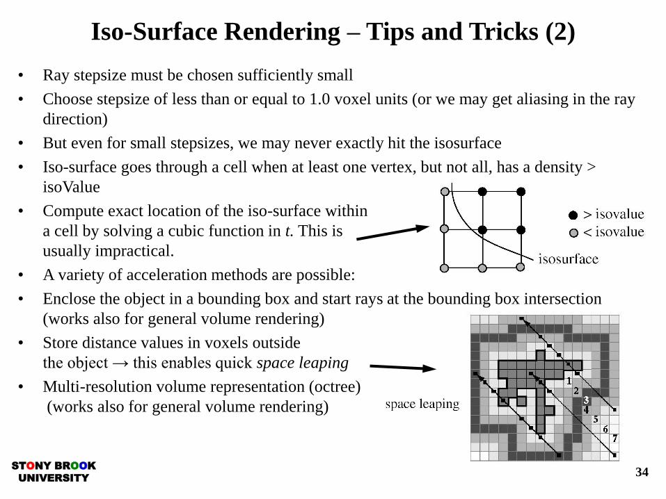
Iso-Surface Rendering – Tips and Tricks (2)

34

• Ray stepsize must be chosen sufficiently small

• Choose stepsize of less than or equal to 1.0 voxel units (or we may get aliasing in the ray

direction)

• But even for small stepsizes, we may never exactly hit the isosurface

• Iso-surface goes through a cell when at least one vertex, but not all, has a density >

isoValue

• Compute exact location of the iso-surface within

a cell by solving a cubic function in t. This is

usually impractical.

• A variety of acceleration methods are possible:

• Enclose the object in a bounding box and start rays at the bounding box intersection

(works also for general volume rendering)

• Store distance values in voxels outside

the object → this enables quick space leaping

• Multi-resolution volume representation (octree)

(works also for general volume rendering)