3DTV rendering from multiple cameras
72
Master‟s Thesis 3D-TV Rendering from Multiple Cameras Thesis committee: Prof. dr. ir. Jan Biemond Dr. C.P. Botha Dr. Emile A. Hendriks Dr. ir. Andre Redert Author Anastasia Manta Email [email protected] Student number 1337424 Thesis supervisor Dr. Emile A.Hendriks Dr.ir. Andre Redert Date November 12, 2008
-
Upload
independent -
Category
Documents
-
view
2 -
download
0
Transcript of 3DTV rendering from multiple cameras

Master‟s Thesis
3D-TV Rendering from Multiple Cameras
Thesis committee: Prof. dr. ir. Jan Biemond
Dr. C.P. Botha
Dr. Emile A. Hendriks
Dr. ir. Andre Redert
Author Anastasia Manta
Email [email protected]
Student number 1337424
Thesis supervisor Dr. Emile A.Hendriks
Dr.ir. Andre Redert
Date November 12, 2008

3DTV Rendering from Multiple Cameras
- 2 -

3DTV Rendering from Multiple Cameras
- 3 -
Preface
This thesis is the final work of my Master study at the Information and Communication Theory group,
Faculty of Electrical Engineering, Mathematics and Informatics, at Delft University of Technology. It serves
as documentation of my work during the graduation, which has been made from February 2008 until
November 2008. This graduation has been preceded by a research assignment on Multiview Imaging and
3DTV during the period October 2007 - January 2008.
Anastasia Manta
Delft, November 2008
Acknowledgements
One year ago, deciding my thesis topic was not an easy task. There were so many things in my mind and a
wide range of different interesting topics to choose from. One year after, I would sincerely like to thank my
supervisors, Emile and Andre, for being really good teachers. I would like to thank them for being supportive
and creative, for our fruitful discussions and for teaching me the way to overcome problems and come up
with new fresh ideas. It was a pleasure working with them.
The ICT group provided a friendly and pleasant environment to work. I would like to thank everybody who
contributed to the nice atmosphere of the group.
Finally, I have to admit that spending two years in TUDelft was an unexpectedly nice experience. I am
grateful to all the people that were part of my experience. Especially my family in Greece, my friends, the
old and the new ones.

3DTV Rendering from Multiple Cameras
- 4 -

3DTV Rendering from Multiple Cameras
- 5 -
Contents
1. Introduction ......................................................................................................................................... - 6 -
a. Three - Dimensional Television (3D TV) ....................................................................................... - 6 -
b. Three-Dimensional Television; a chain of processes .................................................................... - 7 -
c. Problem Statement .......................................................................................................................... - 8 -
2. Related work ...................................................................................................................................... - 10 -
a. Model-based rendering (MBR) – rendering with explicit geometry ......................................... - 10 -
b. Image-based rendering (IBR) – rendering with no geometry ................................................... - 15 -
c. Hybrid techniques – rendering with implicit geometry ............................................................. - 18 -
d. Compatibility with 3DTV applications ........................................................................................ - 25 -
3. Rendering ........................................................................................................................................... - 26 -
a. Basic approach ............................................................................................................................... - 27 -
b. Weighted approach ....................................................................................................................... - 32 -
c. Outlier removal approach............................................................................................................. - 35 -
4. Experimental setup ............................................................................................................................ - 43 -
5. Evaluation .......................................................................................................................................... - 46 -
6. Discussion and Future work ............................................................................................................. - 52 -
b. Future Research ............................................................................................................................. - 53 -
7. Appendix ............................................................................................................................................ - 54 -
A. Results ......................................................................................................................................... - 54 -
B . Clustering experiment ................................................................................................................ - 60 -
C. Depth maps ................................................................................................................................. - 64 -
D. Mean Shift algorithm ................................................................................................................. - 65 -
8. References .......................................................................................................................................... - 69 -

3DTV Rendering from Multiple Cameras
- 6 -
1. Introduction
a. Three - Dimensional Television (3D TV)
As early as the 1920s, TV pioneers dreamed of developing high-definition three-dimensional (3D) color TV,
as only this would provide the most natural viewing experience. During the next eighty years, the early
black-and-white prototypes evolved into high-quality color TV, but the hurdle of 3D-TV still remains.
The term three-dimensional television (3DTV) is understood as a natural extension of two-dimensional
television – which produces a flat image on a screen – into the third dimension. This means that the
impression of the viewer also involves the perception of depth. Our two eyes view the world from slightly
different positions and the two slightly different images registered by our eyes play a primary role in depth
perception. The brain merges this information and creates the perception of a single 3D view. In the absence
of the original scene or object, the same perception can be created by employing systems exploiting this
mechanism.
The advent of three-dimensional television (3D TV) became of relevance in early 1990s with the
introduction of the first digital TV services. The new type of media that expands the user experience beyond
what is offered by now is being developed by the convergence of new technologies from computer graphics,
computer vision, multimedia, and related fields.
Figure 1: Philips' lenticular lens 3-D display requires no special glasses and can show 3-D scenes simultaneously to
several viewers. (Photo:Philips[1])

3DTV Rendering from Multiple Cameras
- 7 -
b. Three-Dimensional Television; a chain of processes
An integrated 3DTV system, involves different building blocks. The main blocks are: capturing of 3D
moving scenes, their representation, rendering, compression and transport, and finally display.
In the entire processing chain there are numerous of challenges [2]. For the acquisition of dynamic scenes, an
array of cameras is needed in most cases. The camera setups range from dense configuration (Stanford Light
Field Camera, [3]) to intermediate camera spacing, [4], and wide camera distribution (Virtualized
RealityTM, [5]).
For applications involving multiple cameras, camera calibration follows the acquisition of the scenes, in
order to guarantee geometric consistency across the different cameras. The purpose of the calibration is to
establish the relationship between 3D world coordinates and their corresponding 2D image coordinates.
Once this relationship is established, 3D information can be inferred from 2D information and vice versa.
From the acquired multiview data, one should consider how to represent a 3D scene in a way that is suitable
for latter processes: rendering, compression and transmission. Methods for 3D scene representation are often
classified as a continuum between two extremes. The one extreme is represented by classical 3D computer
graphics methods. This approach can be called geometry-based modeling, because the geometry of the scene
is described in detail. The other extreme is called image-based modeling and does not use any 3D geometry
at all. Purely image-based representations need many densely spaced cameras.
In the rendering stage, which is interrelated with the 3D representation, new views of scenes are
reconstructed. Depending on the functionality required, there is a spectrum of renderings, from rendering
with no geometry to rendering with explicit geometry. The technologies differ from each other in the amount
of geometry information of the scene.
Having defined the data, efficient compression and coding is the next block in the 3D video processing
chain. There are many different data compression techniques corresponding to different data representations,
[6]. For example, there are different techniques for 3D meshed, depth data etc. The amount of multiview
image data is usually huge, hence the data compressing and the data streaming are challenging tasks.
The display is the last, but definitely not least, significant aspect in the chain of 3D vision. The display is the
most visible aspect of the 3DTV and is probably the one by which the general public will judge its success,
[6]. Two main categories of 3D displays are available, those which imply personal specialized 3D headgear
and those which do not (autostereoscopic displays) [7].

3DTV Rendering from Multiple Cameras
- 8 -
Displays in the first category, using personal headgear, are taking advantage of an obvious way to direct the
views into the user‟s eyes. Examples are head mounted display systems and systems using LCD shutter
glasses. Although these solutions can provide a great immersive 3D experience, the public reluctance to wear
devices is discouraging their mass-market acceptance.
Autostereoscopic displays with tracking rely on real time tracking of the viewer position and projecting the
left and right parts of a stereoscopic video stream into the corresponding user‟s eye. Current trackers and
display optics are suited for a single-user 3D video experience only [8].
The ideal trackingless 3D displays shows so many images in different directions in space, that any viewer at
any position sees different images with his left and right eye. Inherently, such a display serves multiple users,
and provides them not only with stereo imagery but also with the motion parallax cue.
Current multi-view displays such as the Philips 3D-LCD [9] show in the order of 10 images, within a narrow
zone, e.g. 15°, which is repeated over a wider viewing angle to serve multiple viewers.
c. Problem Statement
To enable the use of 3DTV in real-world applications, the entire processing chain as discussed before needs
to be considered. There are numerous challenges in this chain. In addition, there are strong interrelations
between all the processes involved.
In this thesis the focus is set on the generation of the 3D content, and more specifically on the rendering part.
The generation of 3D content is an active research area and lots of research works can be found in the current
literature. First the state of the art methods are compared. Their advantages and disadvantages are discussed.
The investigation of the methods shows that there is still space for improvement and that none of the current
methods can completely accomplish the requirements of a 3DTV application.
We will introduce a new approach that matches better a 3DTV application. The approach is tested on real
data and its feasibility to create 3D content is investigated. A couple of adaptations of the approach are also
discussed.
This report has been structured as follows. The second chapter discusses related work. In this chapter the
special requirements and the equipment available are also discussed and the research question is defined. The
third chapter reviews the different analysis and rendering approaches that were used in the current project,
discussing the steps from one approach to the other and the novelties that each of them introduces. In chapter
four the experimental setup is described. The evaluation of the discussed approaches, objective and

3DTV Rendering from Multiple Cameras
- 9 -
subjective, is presented in chapter five. In chapter six the work conducted during this thesis project is
discussed. Some open issues and ideas for future research are also stated.

3DTV Rendering from Multiple Cameras
- 10 -
2. Related work
Content availability is a factor that influences the success of 3DTV. Content production is a difficult task and
it is even more difficult to create 3D effects in the content that are pleasing to the eye. As discussed before, a
chain of interrelated stages have to be considered in order to enable the generation of 3D content. The
Current literature with focus in the interrelated 3D representation and rendering stages is discussed in this
chapter.
As said before, the methods for 3D scene representation and rendering are often classified as a continuum
between two extremes. Geometry or model-based rendering and image-based rendering . In between the two
extremes a number of methods exist which make use of both approaches and combine their characteristics.
a. Model-based rendering (MBR) – rendering with explicit geometry
Geometry based rendering is used in applications such as games, Internet, TV and movies. The achievable
performance with these models might be excellent, typically if the scenes are purely computer generated.
The available technology for both production and rendering has been highly optimized over the last few
years, especially in the case of common 3-D mesh representations. In addition, state-of-the-art PC graphic
cards are able to render highly complex scenes with an impressive quality in terms of refresh rate, level of
detail, spatial resolution, reproduction of motion, and accuracy of textures [2].
With the use of geometry-based representations quite sparse camera configurations are feasible, but most
existing systems are restricted to foreground objects only [10,11,12] . In other words, despite the advances in
3-D reconstruction algorithms, reliable computation of full 3-D scene models remains difficult. In many
situations, only a certain object in the scene– such as the human body- is of interest. Here, prior knowledge
of the object model is used to improve the reconstruction quality.
Voxel-based representations, [13], can easily integrate information from multiple cameras but are limited in
resolution. The work of Vedula et al., [13], based on the explicit recovery of 3D scene properties, first uses
the so-called voxel coloring algorithm to recover a 3D voxel model of the scene at each time instant. The
non-rigid motion of the scene between consecutive time instants is recovered, Figure 2. In the next stage, the
voxel models and scene flow become inputs to a spatio-temporal view interpolation algorithm.

3DTV Rendering from Multiple Cameras
- 11 -
Figure 2: A set of calibrated images at 2 consecutive time instants. From these images, 3D voxel models are computed
at each time instant using the voxel coloring algorithm. After computing the 3D voxel models, the dense non-rigid 3D
motion or “scene flow” between these models is computed.
A prominent class of geometry reconstruction algorithms is shape-from-silhouette approaches. Shape-from-
silhouette reconstructs models of a scene from multiple silhouette images or video streams. Starting from the
silhouettes extracted from the camera pictures, a conservative shell enveloping the true geometry of the
object is computed by reprojectng the silhouette cones into the 3-D scene and intersecting them. This
generated shell is called the visual hull. While the visual hull algorithms are efficient and many systems
allow for real-time reconstruction the geometry models they reconstruct are often not accurate enough for
high-quality reconstruction of human actors.
Since scenes involving human actors are among the most difficult to reconstruct, research studies focused on
free viewpoint videos of human actors can be found in literature. A typical example is the work of Carranza
et al, [10], recently updated by Theobalt et al. [11], where a triangle mesh representation is employed
because it offers a closed and detailed surface representation. Since the model must be able to perform the
same complex motion as its real-world counterpart, it is composed of multiple rigid-body parts that are
linked by a kinematic chain. The joints between segments are parameterized to reflect the object‟s kinematic
degrees of freedom. Besides object pose, the dimensions of the separate body parts also must be kept
adaptable as to be able to match the model to the object‟s individual stature.
A virtual reality modeling language (VRML) geometry model of a human body is used [Figure 3(a)].
Indicatively, the model consists of 16 rigid body segments, one each for the upper and lower torso, neck and
head; and pairs of the upper arms, lower arms, hands, upper legs, lower legs, and feet. In total, more than
21,000 triangles make up the human body model.

3DTV Rendering from Multiple Cameras
- 12 -
(a) (b) Figure 3: (a) Surface model and the underlying skeletal structure. Spheres indicate joints. (b) Typical camera and light
arrangement during recording.
The challenge in applying model-based analysis for free-viewpoint video reconstruction is to find the way to
adapt the geometry model automatically and robustly to the object‟s appearance as it was recorded by the
video cameras. Since the geometry model is suitably parameterized to alter its shape and pose, the problem
reduces to determining the parameter values that achieve the best match between the model and the video
images. This task is regarded as an optimization problem.
The object‟s silhouettes, as seen from the different camera viewpoints, are used to match the model to the
recorded video images. The foreground in all video images is segmented and binarized. At the same time, the
3-D object model is rendered from all camera viewpoints using conventional graphic hardware, after which
the rendered images are thresholded to yield binary masks of the model‟s silhouettes. Then, the rendered
model silhouettes are compared to the corresponding image silhouettes: as comparison measure, or matching
score, the number of silhouette pixels is used that do not overlap when putting the rendered silhouette on top
of the recorded silhouette. Conveniently, the logical exclusive-or (XOR) operation between the rendered
image and the recorded image yields those silhouette pixels that are not overlapping. By summing over the
non-overlapping pixels for all images, the matching score is obtained. To adapt model parameter values such
that the matching score becomes minimal, a standard numerical nonlinear optimization algorithm runs on the
CPU. For each new set of model parameter values, the optimization routine evokes the matching score
evaluation routine on the graphics card. After convergence, object texture can be additionally exploited for
pose refinement.
One advantage of model-based analysis is the low-dimensional parameter space when compared to general
reconstruction methods (Figure 5): the parameterized 3-D model may provide only a few dozen degrees of
freedom that need to be determined, which greatly reduces the number of potential local minima. Many high-
level constraints are already implicitly incorporated into the model, such as kinematic capabilities.
Additional constraints can be easily enforced by making sure that all parameter values stay within their
anatomically plausible range during optimization.

3DTV Rendering from Multiple Cameras
- 13 -
Figure 4: Analysis-by-synthesis: To match the geometry model to the multiview video footage, the foreground object is
segmented and binarized, and the 3-D model is rendered from all camera viewpoints. The boolean XOR operation is
executed between the reference images and the corresponding model renderings. The number of non-overlapping pixels
serves as matching score. Via numerical optimization, model parameter values are varied until the matching score is
minimal.
Figure 5: From eight video cameras spaced all around the scene, model-based
method can capture the complex motion of a dancer.
After model-based motion capture, a high-quality 3-D geometry model is available that closely, but not
exactly, matches the dynamic object in the scene. For photorealistic rendering results, the original video
footage must be applied as texture to the model. Projective texture mapping is a well-known technique to
apply images as texture to triangle-mesh models. To achieve optimal rendering quality, however, it is
necessary to process the video textures offline prior to real-time rendering [10]: local visibility must be
considered correctly to avoid any rendering artifacts due to the inevitable small differences between model
geometry and the true 3-D object surface. Also, the video images, which are taken from different viewpoints,
must be blended appropriately to achieve the impression of one consistent object surface texture.
Because model geometry is not exact, the reference image silhouettes do not correspond exactly to rendered
model silhouettes. When projecting the reference images onto the model, texture belonging to some frontal
body segment potentially leaks onto other segments farther back [Figure 6(a)]. To avoid such artifacts, each

3DTV Rendering from Multiple Cameras
- 14 -
reference view‟s penumbral region must be excluded during texturing. To determine the penumbral region of
a camera, vertices of zero visibility are determined not only from the camera‟s actual position but also from a
few slightly displaced virtual camera positions [Figure 6(b)]. For each reference view, each vertex is checked
whether it is visible from all camera positions, actual as well as virtual. A triangle is projectively textured
using a reference image only if all of its three vertices are completely visible from that camera.
(a) (b) Figure 6: Penumbral region determination: (a) Small differences between object silhouette
and model outline can cause texture of frontal model segments to leak onto segments
farther back. (b) By projecting each reference image onto the model also from slightly
displaced camera positions, regions of dubious visibility are determined. These are
excluded from texturing by the respective reference image.
Most surface areas of the model are seen from more than one camera. If the model geometry corresponded
exactly to that of the recorded object, all camera views could be weighted according to their proximity to the
desired viewing direction and blended without loss of detail. However, model geometry has been adapted to
the recorded person by optimizing only a comparatively small number of free parameters. The model is also
composed of rigid body elements which is clearly an approximation whose validity varies, e.g., with the
person‟s apparel. In summary, the available model surface can be expected to locally deviate from true
object geometry. Accordingly, projectively texturing the model by simply blending multiple reference
images causes blurred rendering results, and model texture varies discontinuously when the viewpoint is
moving. Instead, by taking into account triangle orientation with respect to camera direction, high-quality
rendering results can still be obtained for predominantly diffuse surfaces [10].
After uploading the 3-D model mesh and video cameras‟ projection matrices to the graphics card, the
animated model is ready to be interactively rendered. During rendering, the multiview imagery,
predetermined model pose parameter values, visibility information, and blending coefficients must be
continuously uploaded, while the view-dependent texture weights are computed on the fly on the GPU.

3DTV Rendering from Multiple Cameras
- 15 -
b. Image-based rendering (IBR) – rendering with no geometry
The other extreme in 3-D scene representation is called image-based rendering and does not use any 3-D
geometry at all. The main advantage is a potentially high quality of virtual view synthesis avoiding any 3-D
scene reconstruction. However, this benefit has to be paid by dense sampling of the real world with a
sufficiently large number of natural camera view images. In general, the synthesis quality increases with the
number of available views. Hence, typically a large number of cameras have to be set up to achieve high-
performance rendering, and therefore a tremendous amount of image data needs to be processed. Contrarily,
if the number of used cameras is too low, interpolation and occlusion artifacts will appear in the synthesized
images, probably affecting the quality.
Examples of image-based representations are ray space or light field [14, 15] and panoramic configurations
including concentric and cylindrical mosaics [16]. The underlying idea in most of these methods is capturing
the complete flow of light in a region of the environment. Such a flow is described by a plenoptic function.
The plenoptic function was introduced by Adelson and Bergen, [17], in order to describe the visual
information available from any point space. It is characterized by seven dimensions, namely the viewing
position (Vx, Vy, Vz), the viewing direction (θ, φ) or (x,y) in Cartesian coordinates , the time t and the
wavelength λ. (l(7)
(Vx, Vy, Vz, θ, φ, λ, t)).
Figure 7: The 7D plenoptic function
The image-based representation stage is in fact a sampling stage, samples are taken from the plenoptic
function for representation and storage. The problem with the 7D plenoptic function is that it is so general
that due to the tremendous amount of data required, sampling the full function into one representation is not
feasible. Research on image-based modeling is mostly about how to make reasonable assumptions to reduce
the sample data size while keeping the rendering quality. One major strategy to reduce the data size is
restraining the viewing space of the viewers. There is a common set of assumptions that people made for
restraining the viewing space. Some of them are preferable, as they do not impact much on the viewers‟
experiences. Some others are more restrictive and used only when the storage size is a critical concern.
By ignoring wavelength and time dimensions, McMillan and Bishop [18] introduced plenoptic modeling,
which is a 5D function:
l(5)
(Vx, Vy, Vz, θ, φ)

3DTV Rendering from Multiple Cameras
- 16 -
They record a static scene by positioning cameras in the 3D viewing space, each on a tripod capable of
continuous panning. At each position, a cylindrical projected image was composed from the captured images
during the panning. This forms a 5D image-based representation: 3D for the camera position, 2D for the
cylindrical image. To render a novel view from the 5D representation, the closeby cylindrical projected
images are warped to the viewing position based on their epipolar relationship and some visibility tests.
The most well-known image-based representations are the light field [15], and the Lumigraph [19] (4D).
They both ignored the wavelength and time dimensions and assumed that radiance does not change along a
line in free space. However parameterizing the space of oriented lines is still a tricky problem. The solutions
they came out happened to be the same: light rays are recorded by their intersections with two planes. One of
the planes is indexed with coordinate (u,v) and the other with coordinate (s,t), i.e.:
l(4)
(s,t,u,v)
In Figure 8, an example where the two planes, namely the camera plane and the focal plane, are parallel is
shown. This is the most widely used setup. An example light ray is shown and indexed as (u0,v0,s0,t0). The
two planes are then discretized so that a finite number of light rays are recorded. If all the discretized points
from the focal plane are connected to one discretized point on the camera plane, we get an image (2D array
of light rays). Therefore, the 4D representation is also a 2D image array, as is shown in Figure 9.
Figure 8: One parameterization of the light field.
Figure 9: A sample light field image array: fruit plate.
The difference between light field and Lumigraph is that light field assumes no knowledge about the scene
geometry. As a result the number of sample images required in light field for capturing a normal scene is

3DTV Rendering from Multiple Cameras
- 17 -
huge. On the other hand, Lumigraph reconstructs a rough geometry for the scene with an octree algorithm to
facilitate the rendering (discussed later on) with a small amount of images. For this reason Lumigraph is
sometimes classified as an hybrid and not a pure image-based modeling technique.
In the rendering stage in order to create a new view of the object, the view is splitted into its light rays, which
are then calculated by quadlinearly interpolating existing nearby light rays in the image array. For example,
the light ray (u0,v0,s0,t0) in Figure 8 is interpolated from the 16 light rays connecting the solid discrete points
on the two planes. The new view is then generated by reassembling the split rays together. Such rendering
can be done in real time and is independent of the scene complexity. Lumigraph, has also the advantage that
can be constructed from a set of images taken from arbitrarily placed viewpoints. A re-binning process is
therefore required. Geometric information is used to guide the choices of the basis functions. Because of the
use of geometric information, sampling density can be reduced.
Other than the assumptions made in light field, concentric mosaics, [16], further restricts that both the
cameras and the viewers are on a plane, which reduces the dimension of the plenoptic function to three. In
concentric mosaics, the scene is captured by mounting a camera at the end of a level beam, and shooting
images at regular intervals as the beam rotates, as is shown in Figure 10. The light rays are then indexed by
the camera position or the beam rotation angle a; and the pixel locations (u, v):
l(3)
(α,u,v).
Figure 10: Concentric mosaic capturing
The rendering of concentric mosaics is slit-based. The novel view is split into vertical slits. For each slit, the
neighboring slits in the captured images are located and used for interpolation. The rendered view is then
reassembled using these interpolated slits. Although vertical distortions exist in the rendered images, they
can be alleviated by depth correction. Concentric mosaics do not require the difficult modeling process of
recovering geometric and photometric scene models. Yet they provide a much richer user experience by
allowing the user to move freely in a circular region and observe significant parallax and lighting changes.
All these methods do not make any use of geometry, but they either have to cope with an enormous
complexity in terms of data acquisition or they execute simplifications restricting the level of interactivity.

3DTV Rendering from Multiple Cameras
- 18 -
c. Hybrid techniques – rendering with implicit geometry
In between the two above extremes, lies rendering with implicit geometry, a truly active research area. When
3D models of the objects and scene are unavailable, like in IBR techniques, user interaction is limited. If
approximate geometry of objects in a scene can be recovered, then interactive editing of real scenes, which is
one of the objectives of 3DTV, is facilitated.
A classical approach is the use of depth or disparity maps. Such maps assign a depth value to each sample of
an image. Together with the original two-dimensional (2-D) image the depth map builds a 3-D-like
representation, sometimes called 2.5-D, [20]. The point where implicit geometry becomes explicit is not very
clear. In this report systems that use geometry information in the form of disparity maps are regarded as
systems with implicit geometry, therefore rendering techniques using depth information are included in this
chapter.
When the depth information is available for every point in one or more images, 3D warping techniques can
be used to render nearby viewpoints. An image can be rendered from any nearby point of view by projecting
the pixels of the original image to their proper 3D locations and re-projecting them onto the new picture. The
most significant problem in 3D warping is how to deal with holes generated in the warped image. Holes are
due to the difference of sampling resolution between the input and output images, and the disocclusion where
part of the scene is seen by the output image but not by the input images. To fill in holes, the most commonly
used method is to splat a pixel in the input image to several pixels in the output image.
Closer to the geometry-based end of the spectrum, methods are reported that use view-dependent geometry
and/or view dependent texture [21]. Instead of explicit 3-D mesh models also point-based representations or
3-D video fragments can be used [22], (ETH).
Waschbusch et al, [22, 23], for example, proposes a view-independent point-based representation of the
depth information. The ETH Institute, which is conducting this research, uses several so-called 3D video
bricks that are capturing high-quality depth maps from their respective. Each brick is movable and contains
one color, two grayscale cameras, and a projector. The matching algorithm used for depth extraction is
assisted by the projectors illuminating the scene with binary structured light patterns. Texture and depth are
acquired simultaneously.
Each brick acquires the scene geometry using depth from stereo algorithm. Depth maps are computed for the
images of the left and right grayscale cameras by searching for corresponding pixels. Stereo matching is
formulated as a maximization problem over an energy which defines a matching criterion of two pixel
correlation windows. An adaptive correlation window is used covering multiple time steps only in the static
part of the correlation windows. For the moving parts discontinuities in the image space are going to be

3DTV Rendering from Multiple Cameras
- 19 -
extended into the temporal domain, making correlation computation more difficult. Therefore the correlation
window is extended in the temporal dimension, only for static parts, to cover three or more images.
Figure 11: The 3D video brick with cameras and projector (left), simultaneously acquiring textures (middle) and
structured light patterns (right)
A two phase post processing is applied to the disparity images. First the regions of wrong disparity are
identified and then new disparities are extrapolated into these regions from their neighbours.
To model the resulting three-dimensional scene, a view-independent, point-based data representation is used.
All reconstructed views are merged into a common world reference frame. Three video bricks were used in
the experiments of paper [23], thus three different views. The model is in principle capable of providing a
full 3600 view if the scene has been acquired from enough viewpoints. It consists of a set of samples, where
each sample corresponds to a point on a surface and describes its properties such as location and color.
Every point is modeled by a three-dimensional Gaussian ellipsoid spanned by the vectors t1, t2, t3, around its
center p. This corresponds to a probabilistic model describing the positional uncertainty of each point by a
trivariate normal distribution:
11( ) ( )
2
3
1( ) ( ; , )
(2 )
Tx p V x p
xp x N x p V e
V
with expectation value p and covariance matrix
1 2 3 1 2 3( ) ( )T
V t t t t t t
composed of 3 x 1 column vectors t1.
Assuming a Gaussian model for each image pixel uncertainty, first the back-projection of the pixel into
three-space is computed which is a 2D Gaussian parallel to the image plane spanned by two vectors tu and tv.
Extrusion into the third domain by adding a vector tz guarantees a full surface coverage under all possible
views. This is illustrated in Figure 12.

3DTV Rendering from Multiple Cameras
- 20 -
Figure 12: Construction of a 3D Gaussian ellipsoid.
Each pixel (u, v) is spanned by orthogonal vectors σu(1,0)T and σv(0,1)
T in the image plane. Assuming a
positional deviation σc, the pixel width and height under uncertainty are σu = σv = 1+σc, σc is estimated to be
the average re-projection error of the calibration routine.
The depth of each pixel is inversely proportional to its disparity d as defined by the equation
L L R
L R
f c cz
d p p
Where fL is the focal length of the rectified camera, cL and cR are the centers of projection, and pL and pR , the
u-coordinates of the principal points. The depth uncertainty σz is obtained by differentiating the above
equation and augmenting the gradient Δd of the disparity with its uncertainty σc:
2( )
( )
L L R
z c
L R
f c cd
d p p
After back-projection the point model still contains outliers and falsely projected samples. Some points
originating from a specific view may look wrong from extrapolated views due to reconstruction errors,
especially at depth discontinuities. In the 3D model, they may cover correct points reconstructed from other
views, disturbing the overall appearance of the 3D video. Thus, those points are removed by checking the
whole model for photo consistency with all texture cameras.
In the rendering stage they adopt an interesting approach described by Broadhurst et al., [24]. Broadhurst
uses probabilistic volume ray casting to generate smooth images. Each ray is intersected with the Gaussians
of the scene model. At a specific intersection point x with the sample i, the evaluation N(x;pi;Vi) of the
Gaussian describes the probability that a ray hits the corresponding surface point. To compute the final pixel
color, two different approaches are described. The maximum likelihood method associates a color with the
ray using only the sample which has the most probable intersection. The second approach employs the Bayes
rule: it integrates all colors along each ray weighted by the probabilities without considering occlusions.
Thus, the color of a ray R is computed as:

3DTV Rendering from Multiple Cameras
- 21 -
The maximum likelihood method generates crisp images, but it also sharply renders noise in the geometry.
The Bayesian approach produces very smooth images with less noise, but is incapable of handling occlusions
and rendering solid surfaces in an opaque way. The rendering method that the authors propose combines
both approaches in order to benefit from their respective advantages. The idea is to accumulate the colors
along each ray like in the Bayesian setting, but to stop as soon as a maximum accumulated probability has
been reached. Reasonably, a Gaussian sample should be completely opaque if the ray passes its center. The
line integral through the center of a three-dimensional Gaussian has a value of 1/2π and for any ray R it holds
that:
Thus, they accumulate the solution of the integrals of the above equation by traversing along the ray from the
camera into the scene and stop as soon as the denominator of the equation reaches 1/2π. Assuming that solid
surfaces are densely sampled, the probabilities within the surface boundaries will be high enough so that the
rays will stop within the front surface.
The results of comparison of this approach with the maximum likelihood and Bayesian rendering on noisy
data are demonstrated in Figure 13. The large distortions in the maximum likelihood image, get smoothed
out by the other two methods. However, the Bayesian renderer blends all the points including those from
occluded surfaces, while current method renders opaque surfaces and maintains the blending.
Figure 13: Comparison of maximum likelihood (left) and Bayesian rendering
(center) with Waschbusch et al.‟s approach (right).
A representative result of the method is shown in Figure 14, where novel views of the acquired scene are
rendered with the reconstructed 3D model. A sample video can be found in [25].
( ; , )
( ; , )
i i i
R
i i
i
x R
i
x R
c N x p V
cN x p V
1( ; , )
2x R
N x p V

3DTV Rendering from Multiple Cameras
- 22 -
Figure 14: Re-renderings of the 3D video from novel viewpoints.
The model is in principle capable of providing a full 3600 view if the scene has been acquired from enough
viewpoints. Compared to mesh-based methods, points provide advantages in terms of scene complexity
because they reduce the representation data and do not carry any topological information, which is often
difficult to acquire and maintain. As each point in the model has its own assigned color, they also do not
have to deal with texturing issues. Moreover, a view-independent representation is very suitable for 3D video
editing applications since tasks like object selection can be achieved easily with standard point processing
methods.
The point based data representation model is in general suitable for 3DTV applications but still contains
many redundancies. Big clusters of outliers tend to grow in the discontinuity optimization stage if they
dominate the correct depths in a color segment. Furthermore as the authors acclaim the resulting image
quality could also be improved by exploiting inter-brick correlation and eliminating remaining artifacts at
silhouettes using matting approaches as done by Zitnick et al. [4].
Zitnick et al., [4], propose a quite sophisticated representation. First, guided by the fact that using a 3D
impostor or proxy for the scene geometry can greatly improve the quality of the interpolated views, they
generate and add per-pixel depth maps (multiple depth maps for multiple views). However, even multiple
depth maps still exhibit artifacts (at the rendering stage) when generating novel views. This is mainly
because of the erroneous assumption at the stereo computation stage, that each pixel has a unique disparity.
This is not the case for pixels along the boundary of objects that receive contributions from both the
foreground and background colors.
Zitnick addresses this problem using a novel two-layer representation inspired by Layered Depth Images
[26]. The two layer representation is one of the most efficient rendering methods for 3D objects with
complex geometries and it was proposed already in 1998 by Shade et al.
A Layered Depth Image is an array of layered depth pixels ordered from closest to furthest from a so-called
LDI camera. Each layered depth pixel contains multiple depth pixels at per-pixel location. The farther depth
pixels, which are occluded from the viewpoint at the center of LDI camera, will appear as the viewpoint

3DTV Rendering from Multiple Cameras
- 23 -
moves away from the center of LDI camera. This image-based rendering technique is an abstract of depth
images, which assigns a z-value in addition to the x and y values normally associated with a pixel.
When rendering from an LDI, the requested view can move away from the original LDI view and expose
surfaces that were not visible in the first layer. The previously occluded regions may still be rendered from
data stored in some later layer of a layered depth pixel.
Figure 15: Layered Depth Image (LDI) and LDI camera
There are two ways to generate an LDI from natural images: generate LDI from multiple depth images and
generate LDI from real images directly [26], illustrated as in Figure 15. If multiple color and depth images
from natural images are obtained, the LDI is constructed by warping pixels in other camera locations, such as
C1 and C2. Otherwise, The LDI can be generated directly from the input images by an adaptation of Seitz
and Dyers voxel coloring algorithm [27]. The voxel coloring method assigns colors to voxels (points) in a
3D volume so as to achieve consistency with a set of basis images. In [27], a ordinal visibility constraint is
exploited in order to simplify visibility relationships. In particular, it becomes possible to partition the scene
into a series of voxel layers that obey a monotonic visibility relationship: for every input image, voxels only
occlude other voxels that are in subsequent layers. Consequently, visibility relationships are resolved by
evaluating voxels one layer at a time.
The voxel coloring algorithm visits each of the N3 voxels exactly once and projects it into every image.
Therefore, the time complexity of voxel coloring is O(N3n), where n the number of images. Such a
complexity prohibits the use of the algorithm for the modeling of a whole scene.
Zitnick, [4], overcomes this constraint, by calculating the matting, or second layer information, in specific
areas and not for the whole scene. Matting information is computed within a neighbourhood of four pixels
from all depth discontinuities. A depth discontinuity is defined as any disparity jump greater than λ (=4)
pixels. Within these neighborhoods, foreground and background colors along with opacities (alpha values)
are computed using Bayesian matting [28]. The foreground information is combined to form the boundary
layer as shown in Figure 16. The main layer consists of the background information along with the rest of the

3DTV Rendering from Multiple Cameras
- 24 -
image information located away from the depth discontinuities. Chuang et al.„s algorithm do not estimate
depths, only colors and opacities. Depths are estimated by using alpha-weighted averages of nearby depths in
the boundary and main layers. To prevent cracks from appearing during rendering, the boundary matte is
dilated by one pixel toward the inside of the boundary region.
Figure 16: Two-layer representation: (a) discontinuities in the depth are found and a boundary strip is created around
these; (b) a matting algorithm is used to pull the noundary and main layers Bi and Mi (The boundary layer is drawn
with variable transparency to suggest partial opacity values)
Figure 17 shows the results of applying the stereo reconstruction and two-layer matting process to a
complete image frame. It is noticeable that only a small amount of information needs to be transmitted to
account for the soft object boundaries, and how the boundary opacities and boundary/main layer colors are
cleanly recovered.
Figure 17: Sample results from matting stage: (a) main color estimates; (b) main depth estimates; (c) boundary color
estimates; (d) boundary depth estimates; (e) boundary alpha (opacity) estimates. For ease of printing the boundary
images are negated, so that transparent empty pixels show up as white.
In the rendering stage, given a novel view, the nearest two cameras in the data set are picked. For each
camera the main data and boundary data are projected into the virtual view. The results are stored in separate
buffers each containing color, opacity and depth. These are then blended to generate the final frame.
The layered depth image approach, provides results with quite good visual quality. However, even for an
approach like Zitnick‟s dense scene sampling is necessary. For example in order to achieve coverage about
30o
, a configuration of 8 cameras was used. The discussed approach processes each camera independently
from the others. Better quality could be obtained by merging data from adjacent views when trying to
estimate the semi-occluded background. This would also allow the multi-image matting to get even better
estimates of foreground and background color and opacities.

3DTV Rendering from Multiple Cameras
- 25 -
d. Compatibility with 3DTV applications
This thesis addresses several problems and constraints discussed here. Motivation to test a new approach
emanates from the special requirements that a 3DTV application has. The fact that the 3D video should
include not only the foreground objects but also the background is considered as a premise.
The flexibility and scalability, important characteristics of an efficient approach, motivate the use of a per-
pixel algorithm. Per-pixel operations allow flexibility in the sense that their complexity depends on the
resolution of the initial images. Therefore, computational cost could be decreased by using low quality
images, or increased when high resolution initial images are used. The scalability is important, in the sense
that more cameras can be added, and in this case the algorithm preserves its characteristics but the quality of
the final result is refined, or a wider view range is feasible. Parallel computation, that is feasible for
independent per-pixel operations, could also facilitate a real time system.
The approaches discussed in chapter three are also motivated from the limited recording facilities (low
number of cameras) available in the studio at the university. An approach that would be able to generate a
3D video captured initially by four stereo cameras, of 640x480 resolution, was a challenging task
considering the current literature studies demanding dense camera configurations. Motivated from 3DTV
requirements and state of the art limitations is therefore the work presented in the next chapters of this thesis
project.
3DTV Rendering from Multiple Cameras
- 26 -
3. Rendering
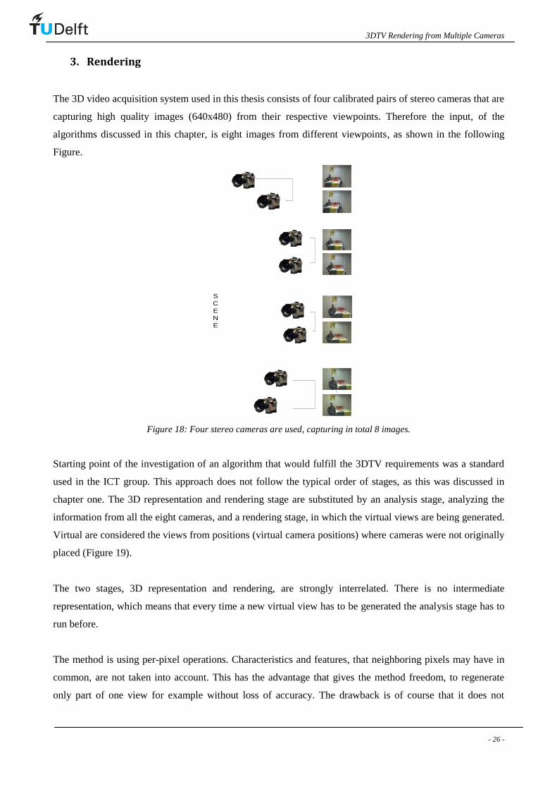
The 3D video acquisition system used in this thesis consists of four calibrated pairs of stereo cameras that are
capturing high quality images (640x480) from their respective viewpoints. Therefore the input, of the
algorithms discussed in this chapter, is eight images from different viewpoints, as shown in the following
Figure.
S
C
E
N
E
Figure 18: Four stereo cameras are used, capturing in total 8 images.
Starting point of the investigation of an algorithm that would fulfill the 3DTV requirements was a standard
used in the ICT group. This approach does not follow the typical order of stages, as this was discussed in
chapter one. The 3D representation and rendering stage are substituted by an analysis stage, analyzing the
information from all the eight cameras, and a rendering stage, in which the virtual views are being generated.
Virtual are considered the views from positions (virtual camera positions) where cameras were not originally
placed (Figure 19).
The two stages, 3D representation and rendering, are strongly interrelated. There is no intermediate
representation, which means that every time a new virtual view has to be generated the analysis stage has to
run before.
The method is using per-pixel operations. Characteristics and features, that neighboring pixels may have in
common, are not taken into account. This has the advantage that gives the method freedom, to regenerate
only part of one view for example without loss of accuracy. The drawback is of course that it does not

3DTV Rendering from Multiple Cameras
- 27 -
consider properties of neighboring pixels that could be useful and save computational load in an object-based
approach for example.
a. Basic approach In order to generate a new view, at a virtual position a ray tracing scheme is adopted. Every pixel of the
virtual view is considered independently. Figure 19 is illustrating the method with a one pixel example. This
pixel comes from a depth position in the 3D scene. In order to figure out its depth position different depth
values are tested.
This is conducted as follows: a light ray is constructed for the pixel under consideration. The ray is modeling
all possible depths of the pixel. Therefore it should be able to model all the depth positions possible in the
original 3D scene. A step for the depth is selected. For the whole range of depths, one depth-step at a time
from the virtual view‟s pixel is projected to all the original images. The pixels on which is projected are the
corresponding pixels for the given depth.
.
105cm
220cm
Figure 19: Here two different depth hypotheses (105cm, 220cm) are projected to the original images.

3DTV Rendering from Multiple Cameras
- 28 -
The pixel in every original image matching the given depth should have an RGB value. In case the projection
of a depth does not correspond to a pixel within the borders of the original image then this original image is
not considered effective and is not participating in the regeneration of the virtual view.
By collecting the RGB values, a set of Ncamsx3 values is formed, where Ncams the number of effective
cameras. The mean value, , and the variance, 2 , of the color in this dataset are computed for each of the
three color components:
zNcam
zk
z
Ncam
c
c
k
1
(1)
z
zNcam
zk
zk
Ncam
c
c
k
21
2
2
(2)
where bgrk ,, , and r stands for the red color component, g for the green and b for the blue. Ncam stands
for the number of effective cameras, and c is the index of the cameras. The r, g, b color variances are then
summed up:
zRGB
2 z
r
2 + z
g
2 + z
b
2 (3)
The RGB color variance as it appears in equation 3 is calculated for every step of the ray, or in other words
for every depth hypothesis. In case the depth hypothesis is correct the variance should have a low value. This
happens because for the correct depth, the original cameras should be in agreement, since they should be
viewing the same scene point, and the collected RGB values should converge. A high variance implies
disagreement among the cameras, and is not in general the case of a correct depth.
Therefore from all the depth hypotheses, the one with the lowest variance is selected.
)(min2
zz RGBz
SEL (4)
For this depth the mean RGB value of all the effective cameras is assigned to the new pixel.
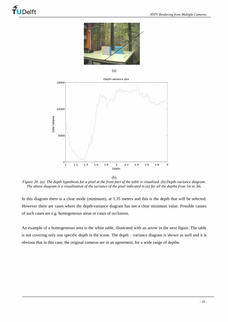
The computed variance for one pixel in a virtual view as a function of possible depths is plotted in Figure 20.
The pixel under consideration is a pixel at the front part of the scene, on the table.
3DTV Rendering from Multiple Cameras
- 29 -
(a)
1 1.2 1.4 1.6 1.8 2 2.2 2.4 2.6 2.8 30
5000
10000
15000
Depth
Col
or V
aria
nce
Depth-variance plot
(b)
Figure 20: (a): The depth hypothesis for a pixel at the front part of the table is visualized. (b):Depth-variance diagram.
The above diagram is a visualization of the variance of the pixel indicated in (a) for all the depths from 1m to 3m.
In this diagram there is a clear mode (minimum), at 1.35 meters and this is the depth that will be selected.
However there are cases where the depth-variance diagram has not a clear minimum value. Possible causes
of such cases are e.g. homogeneous areas or cases of occlusion.
An example of a homogeneous area is the white table, illustrated with an arrow in the next figure. The table
is not covering only one specific depth in the scene. The depth – variance diagram is shown as well and it is
obvious that in this case, the original cameras are in an agreement, for a wide range of depths.

3DTV Rendering from Multiple Cameras
- 30 -
(a)
1 1.2 1.4 1.6 1.8 2 2.2 2.4 2.6 2.8 30
0.5
1
1.5
2
2.5
3x 10
4
Depth
Col
or V
aria
nce
Depth-variance plot
(b)
Figure 21: (a): The depth hypothesis for a pixel on the white table is visualized. (b): Depth-variance diagram. The
above diagram is a visualization of the variance of the pixel indicated in (a) for all the depths from 1m to 3m.
The depth that is going to be selected by the algorithm may not be the correct one. It would be the one with
the lowest variance, but in this case this is not a safe criterion. In Figure 22, the mean RGB values, as they
were calculated for every depth are also plotted. For depth from 1.2 meters to 3 meters the color is white,
with some small changes probably due to illumination changes. Although the selected depth could be wrong,
the color of the pixel in the regenerated view is going to be correct.

3DTV Rendering from Multiple Cameras
- 31 -
(a)
1 1.2 1.4 1.6 1.8 2 2.2 2.4 2.6 2.8 30
0.5
1
1.5
2
2.5
3x 10
4
Depth
Col
or V
aria
nce
(b)
Figure 22: (a): The depth hypothesis for a pixel on the white table is visualized. (b) Depth-variance diagram for the
pixel indicated in for all the depths from 1m to 3m. (a). The dots scattered in the diagram indicate the mean RGB value
for each depth.
Therefore homogeneous areas may are responsible for errors in the depth map of the scene but are not
causing any artifacts in the final image.
The occlusion problem occurs when part of the objects which constitute the scene, or part of the background
is covered by other objects. In this application where multiple cameras are used, occluded areas can be
present at some of the images captured by the original cameras or even in all of them. This causes spread
within the set of the collected RGB values.
A pixel between the two boxes at the right is selected and its depth-variance results are visualized. The
original cameras seem not to agree for the RGB values corresponding to pixels in this area. The cause of the
disagreement is that for some of the 8 original cameras the purple box is occluding the background, for some

3DTV Rendering from Multiple Cameras
- 32 -
of them the stripped box is occluding the background and there are also those cameras which are capturing
the background. The depth hypothesis is therefore not valid, since the correct depth may be not the one with
the lowest variance.
(a)
1 1.2 1.4 1.6 1.8 2 2.2 2.4 2.6 2.8 32000
4000
6000
8000
10000
12000
14000
Depth
Col
or V
aria
nce
Depth-variance plot
(b)
Figure 23: (a): The depth hypothesis for a pixel at the background is visualized. (b):Depth-variance diagram. The
above diagram is a visualization of the variance of the pixel indicated in (a) for all the depths from 1m to 3m.
b. Weighted approach In order to overcome the problem of occlusion, and make the discussed approach compatible with the
regeneration of occluded areas, the proximity of the original cameras to the virtual view is considered.
In current literature camera proximity has been widely used. In the work of Min et al. for example [29],
given a viewpoint the nearest two images (camera i and i+1) are selected and projected into virtual view.
Smolic et al. as well in [30], using a multicamera setup, are building 3D video objects. In order to project the
textures from the original views onto the geometry, voxel models, they are calculating a weight. For each
projected texture a normal vector ni is defined pointing into the direction of the original camera. For

3DTV Rendering from Multiple Cameras
- 33 -
generation of a virtual view into a certain direction vVIEW a weight is calculated for each texture, which
depends on the angle between vVIEW and ni.
The weighted interpolation ensures that at original camera positions the virtual view is exactly the original
view. The closer the virtual viewpoint is to an original camera position the greater the influence of the
corresponding texture on the virtual view.
The approach discussed at the beginning of this chapter is therefore adapted in order to integrate the original
camera – virtual view position proximity. Every time a virtual view at a new position is calculated, a weight
is assigned to every original camera:
422210)()()((
1
vvcvvcvvc
czzyyxx
w (5)
Where (xvv, yvv, zvv) is the position of the virtual view, and (xc, yc, zc) the position of the original camera c.
The weight is different for every, of the c =[1, 8], original cameras. When the distance approaches zero, the
weight gets a great value, but it can never approach infinity, due to the 4
10
factor. We assumed that the
minimum distance between a camera and a virtual view is 1cm=10-2
. So, the squared minimum distance
gives the factor4
10
. In case the projection to one of the cameras is not effective, it is projected out of
borders as already discussed this camera is assigned a zero weight.
The weights of the cameras are participating in the calculation of color variance. The color variance is now
calculated as follows:
8
1
8
1
,
)(
)(
c
c
c
cc
kWEIGHT
w
zkw
z
(6)
2
,8
1
8
1
2
2
,
)(
)(kWEIGHT
c
c
c
cc
kWEIGHT
w
zkw
z
(7)
where bgrk ,, .
The r, g, b weighted color variances are then summed up:
)(2
,z
RGBWEIGHT )(
2
,z
rw + )(
2
,z
gw + )(
2
,z
bw (8)

3DTV Rendering from Multiple Cameras
- 34 -
The weighted color variance is calculated for every depth hypothesis. The depth with the lowest variance is
selected:
)(min
2
,,zz
RGBWEIGHTz
SELWEIGHT
(9)
and its the mean RGB value as calculated in (6) is assigned to the pixel.
The depth-variance diagram, influenced from the camera proximity is shown in the next figure, for a pixel in
the area with occlusion, between the two boxes.
(a)
1 1.2 1.4 1.6 1.8 2 2.2 2.4 2.6 2.8 32000
4000
6000
8000
10000
12000
14000
Depth
Col
or V
aria
nce
Depth-variance plot
erroneous
foreground
(b)

3DTV Rendering from Multiple Cameras
- 35 -
1 1.2 1.4 1.6 1.8 2 2.2 2.4 2.6 2.8 3600
800
1000
1200
1400
1600
1800
2000
2200
Depth
Col
or V
aria
nce
Depth-variance plot
correct
background
(c)
Figure 24: (a): The depth hypothesis for a pixel at the background is visualized.(b,c):Depth-variance diagrams. The
diagrams are visualizations of the variance of the pixel for all the depths from 1m to 3m. (b) non-weighted variance, (c)
weighted variance.
In Figure 24, the depth variance diagram for the first approach discussed in chapter 3.a and the weighted
variance diagram are illustrated. The pixel under consideration is between the two boxes and it belongs to
the background. When the first approach is used (Figure 24.b), the lowest variance is around 1.4 meters. This
depth corresponds to the box and is erroneously selected. In the weighted approach the cameras at positions
close to the virtual view have a stronger impact on the variance. The lowest variance is now detected for
depths around 2.2 meters (depth that corresponds to the background).
c. Outlier removal approach
The weighted approach could solve the occlusion problem but only partially. There are still artifacts
appearing in the regenerated images. In case of occlusion, or in case of illumination changes for example, it
can happen that the cameras are viewing different colors even for the correct depth. An insight on the values
of the cameras for pixels with erroneous colors, shows that the main cause of the errors is the existence of
outlier values.
Taking as an example a second pixel, neighboring to the one appearing in Figure 24, thus within the
occluded area, it turns out that for this pixel the weighted approach is not working.

3DTV Rendering from Multiple Cameras
- 36 -
1 1.2 1.4 1.6 1.8 2 2.2 2.4 2.6 2.8 33000
4000
5000
6000
7000
8000
9000
10000
Depth
Col
or V
aria
nce
Depth-variance plot
erroneous
foreground
(a)
1 1.2 1.4 1.6 1.8 2 2.2 2.4 2.6 2.8 3500
1000
1500
2000
2500
3000
3500
4000
4500
5000
Depth
Col
or V
aria
nce
Depth-variance plot
erroneous
foreground
(b)
Figure 25: Depth-variance diagrams of a pixel in the occluded area. The diagrams are visualizations of the variance of
the pixel for all the depths from 1m to 3m. (a) non-weighted variance, (b) weighted variance.
Although the weights influence the variance of the cameras, the depth with the lowest v is erroneously
around 1.6 meters (the ground truth lies around 2.2 meters). A plot of the RGB values of the eight cameras
indicates the cause of the error:

3DTV Rendering from Multiple Cameras
- 37 -
Figure 26: The dots in the diagram stand for the colors of the eight cameras, for depth 2.2 meters. The color of the dot
represents the RGB color of the camera. The dots are plotted in the RG space.
For the correct depth four of the cameras are viewing the stripped box, one of them the purple box and the
rest three cameras the background. The variance is calculated for all the cameras, therefore if outliers are
present for the correct depth, this is not going to be selected by the algorithm. Probably there will be another
depth value for which the camera values would be less spread.
Solution to this cause of errors is the removal of the outlier values. There are plenty of methods for the
removal of the outliers. A binary classification of the input data into inlier and outlier class could be achieved
with RANSAC, [31], or major vote method. Hard clustering, assigns each data point (feature vector) inside
with a degree of membership equal to one or outside the cluster, with a degree of membership zero.
In our application the borderline between inliers and outliers is not crisp. There is much controversy on what
constitutes an outlier. The borderline depends on the specific scene, and could have a strong effect on the
sharpness of the final image.
In order to have the flexibility to handle such situations, by adapting the parameters of the algorithm for
example, a non –binary clustering algorithm without a priori assumptions on the number of clusters is used.
The method used resembles the mean shift algorithm, an algorithm used broadly in image processing
applications, for image segmentation for example, [32], (Appendix D). The mean shift and the algorithm
used here as well are unsupervised. The clusters and the outliers are identified using an iterative scheme.
The location of the cluster centroids is not known a priori. Here, the mean value of the RGB values as
calculated in (4), (the weights of the cameras are not used here), is the starting vector t
O .The index t stands
for the number of iterations (t>0).

3DTV Rendering from Multiple Cameras
- 38 -
The RGB values of each of the eight cameras, are represented by a vector Vc,. ,(c [1,8] stands for the
number of the camera). Vc is therefore a 3x1 vector, containing information for the three color components
of camera c. The eight Vc vectors constitute the dataset of the algorithm.
The distance, t
cd ,of the initial mean value
tO , with respect to each vector Vc is calculated as:
2
)()()( zVzOzdc
tt
c
(10)
and is an estimate of the variance of the Vc values.
The cameras for which the distance is high are considered outliers, whereas those with low distance value are
considered inliers. Therefore a scalar weight is assigned to each of them, computed as the inverse of the sum
of the distances plus a indicating the minimum acceptable size of a cluster:
)(
1)(
zdzw
t
c
t
cOUTR (11)
The weights of the cameras are normalized, and a new vector for the next iteration is defined as:
8
1
1)()()(
c
c
t
cOUTR
tzVzwzO (12) , with
8
1
1)(
c
t
cOUTRzw (13)
The distance of the starting value O from the vectors Vc is calculated again, new weights are assigned to the
cameras and the starting value O is recomputed with the new camera weights.
The iterative procedure stops when a predefined number of iterations are executed. The sequence of points
should finally converge to one of the so-called attractors of the iterative scheme. This is the final centroid of
the cluster.
With the method described above, none of the cameras has a zero weight. Even the cameras that are
considered outliers are assigned a very small weight which may practically exclude them from the
calculation of centroid of the cluster (the final RGB mean value).
At the end of the iterative process a number indicating the number of the cameras that are practically
participating in the calculation of the mean value (effective number of member-cameras) is computed.
8
1
)(log)(
)( c
cOUTRcOUTR zwzw
ezN (14)
where
cOUTRcOUTR
ww , the weights after the iterations.

3DTV Rendering from Multiple Cameras
- 39 -
There are different ways to integrate the outlier removal method in the sequence of processes. One possible
scenario, is first to select the depth, using the approach discussed at chapter 3.a, based on the color variance
(the camera proximity weights may be used as well). Then for the selected depth, which probably contains
outlier values, the outlier removal method can be performed. The mean value RGB value, the value that
would be finally assigned to the pixel, would be recalculated without the outliers.
This approach saves computational cost, since the outlier removal method which is quite expensive is
executed only once for every pixel. However, is non-optimal. The initial RGB values and the color variances
calculated for all the depths include outliers. A less compromising scenario, in terms of accuracy and
correctness of the final result, is to use the outlier removal method for all the possible depths before the
calculation of the variance.
Therefore what we investigated is first to remove the outliers from the set of the RGB values of the original
cameras and then proceed with the selection of the depth.
In more detail, given a pixel and a depth, the outlier removal method outputs weights for all the cameras,
cOUTRw . These weights can be used to calculate the new mean and variance (non-weighted outlier removal
approach). Only removing the outliers was tested and did not give sufficient results therefore the outlier
removal weights have been linearly combined with the camera proximity weights, c
w (weighted outlier
removal), as calculated in (6):
ccOUTRcFINALwzwzw 7.0)()( (15)
The 0.7 factor was assigned to the camera proximity weights based on experimental observations and the fact
that their influence should not overcome the outlier removal weights.
The mean RGB value is recalculated based on the new combined weights of the cameras. The variance of the
eight RGB values from the center of the cluster (the new mean value) also.
8
1
8
1
,
)(
)(
c
cFINAL
c
cFINALc
kFINAL
w
zkw
z
(16)
2
8
1
8
1
2
2
,
)(
)(kFINAL
c
cFINAL
c
ccFINAL
kFINAL
w
zkw
z
(17)
3DTV Rendering from Multiple Cameras
- 40 -
where bgrk ,, .
Both the variance and the number of effective cameras, as calculated in 14, are used as criterions in the
selection of the depth. The number of effective cameras is used to prevent selection of depths for which very
few cameras are considered inliers. This can happen in case the values are randomly distributed in the RGB
space. Then the outlier removal method could choose one or two observations as inliers, having also a very
low variance. This is general not the correct case so the selection of clusters with few members is stopped, in
the following way.
Starting from the lowest depth, the first local minimum variance is selected and it is only replaced if a lower
variance with a higher number of cameras is present for a higher depth. The reason that the scanning
procedure starts from the lower depths to the higher ones is that we want to select the first visible object
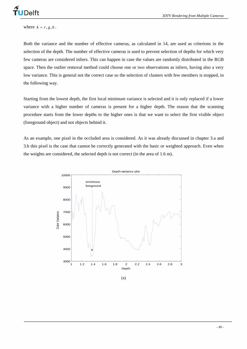
(foreground object) and not objects behind it.
As an example, one pixel in the occluded area is considered. As it was already discussed in chapter 3.a and
3.b this pixel is the case that cannot be correctly generated with the basic or weighted approach. Even when
the weights are considered, the selected depth is not correct (in the area of 1.6 m).
1 1.2 1.4 1.6 1.8 2 2.2 2.4 2.6 2.8 33000
4000
5000
6000
7000
8000
9000
10000
Depth
Col
or V
aria
nce
Depth-variance plot
erroneous
foreground
(a)

3DTV Rendering from Multiple Cameras
- 41 -
1 1.2 1.4 1.6 1.8 2 2.2 2.4 2.6 2.8 3500
1000
1500
2000
2500
3000
3500
4000
4500
5000
Depth
Col
or V
aria
nce
Depth-variance plot
erroneous
foreground
(b)
1 1.5 2 2.5 30
10
20
30
40
50
60
70
80
90
100
Depth
Col
or V
aria
nce
Depth-variance plot
1 cam
2 cams
3 cams
4 cams
5 cams
correct
background
(c)
Figure 27: Depth-variance diagrams of a pixel in the occluded area. The diagrams are visualizations of the variance of
the pixel for all the depths from 1m to 3m. (a) non-weighted variance, (b) weighted variance, (c) variance after the
removal of outliers.
In the above diagram the blue line is the color variance diagram, after the outlier removal. The colorful dots
indicate the number of the effective number of cameras (N). In this example the combination of a low
variance and a high number of camera members happens for a depth around 2.4 meters. In this case the
outlier removal method works for the occlusion problem.

3DTV Rendering from Multiple Cameras
- 42 -
There are still cases for which this approach would not work. When the majority of the cameras are viewing
the wrong color, and the minority the correct, the outlier removal approach will consider inliers the wrong
values. The real inliers will be excluded from the calculation of the final color of the pixel. In such a case
that the correct values are excluded the result is worse than the one of the basic or the weighted approach.

3DTV Rendering from Multiple Cameras
- 43 -
4. Experimental setup
The presented experimental setup uses a pair-wise multi-view camera setup of 8 views, whereas the cameras
are mounted without any geometric restrictions. Video frames are recorded at a resolution 640x480 at 15 fps.
Figure 28: Experimental setup.
Before the recording of the scene, the cameras were calibrated.The camera calibration step is an
integral part of the process of 3D video acquisition. It is determining the internal camera geometric
and optical characteristics (intrinsic parameters) and the 3D position and orientation of the camera
frame relative to a word coordinate system (extrinsic parameters). This step is necessary to
quarantee geometric consistency across the different terminals.
A calibration plate containing 47 dots was captured in four different positions and an minimum
energy calibration algorithm, as proposed by Redert et al. at [33], was used.

3DTV Rendering from Multiple Cameras
- 44 -
Figure 29: Calibration plate placed in four different positions for the calibration algorithm.
After the calibration step, each of the cameras captured one image from a different viewpoint. The recorded
scene is stationary. The algorithm has been tested in stationary scenes; however it can be also used for video
sequences. In this case each frame is reconstructed independently from the previous ones therefore the
temporal characteristics of a video are not taken into account.
Different scenes were recorded, with different backgrounds, simple and more complex ones, people or just
objects.
(a) (b)
(c) (d)

3DTV Rendering from Multiple Cameras
- 45 -
(e) (f)
(g) (h)
Figure 30: Captured scenes with different sceneries.
From the above scenes, two were selected to serve as the scenes in which the algorithms will be tested. A
scene with a colorful, complex background and four boxes and a scene with a simple background and a
human, were chosen. From now on the first scene is referred as four boxes scene (Figure 30.d), and the
second one as coffee scene (Figure 30.g). In both scenes there are objects occluding the background or other
objects so the handling of occlusions can be also assessed.
Professional lighting equipment was not used. The lighting of the room where the recordings took place is
the normal ceiling lighting. Changes in illumination are present in the scene.

3DTV Rendering from Multiple Cameras
- 46 -
5. Evaluation
Objective evaluation of image and video quality is important for image processing systems. The quality
assessment is by itself a wide research area, having as a goal to design algorithms for objective evaluation of
quality in a way that is consistent with subjective human evaluation. By “consistent” it is meant that the
algorithm‟s assessment of quality should be in close agreement with human judgments, regardless of the type
of distortion corrupting the image, the content of the image, or strength of distortion.
In the image coding and computer vision literature, the most frequently used measures are deviations
between the original and coded images, with varieties of the mean square error (MSE) or signal-to-noise
ratio (SNR) being the most common measures [34-36]. The reason for their widespread popularity is their
mathematical tractability. However they do not necessarily correspond to all aspects of the observer‟s visual
perception of the errors, [34, 35], nor do they correctly reflect structural coding artifacts.
For multimedia applications, there has been an increase in the use of quality measures based on human
perception [37-42] Since a human observer is the end user in multimedia applications, an image quality
measure that is based on a human vision model seems to be more appropriate for predicting user acceptance
and for system optimization. This class of distortion measure in general gives a numerical value that will
quantify the dissatisfaction of the viewer in observing the reproduced image in place of the original. The
alternative is the use of subjective tests in which subjects view a series of reproduced images and rate them
based on the visibility of the artifacts. Subjective tests are tedious, time consuming and expensive, and the
results depend on various factors such as the observer‟s background, motivation, etc., and actually only the
display quality is being assessed.
An objective evaluation although not being the optimal one is usually part of the testing of an image
processing technique. In this thesis, PSNR (peak signal-to-noise ratio) is used. The derivative signal to
noise ratio, a criterion that considers the sensitivity of the human eye in the edge information is also
computed. A subjective evaluation, based on the author‟s visual interpretation is finally discussed.
Different approaches exist for computing PSNR of a color image. One simple approach is to calculate the
metrics for the three R,G,B components and then average them. But, the human eye is most sensitive to
intensity information. Therefore the image is first converted to a color space that separates the intensity
channel, here YCbCr. The Y (luma), in YCbCr represents a weighted average of R, G, and B. G is given the
most weight, again because the human eye perceives it most easily. With this consideration, the PSNR is
computed only on the luma channel.
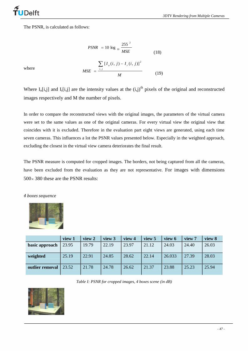
3DTV Rendering from Multiple Cameras
- 47 -
The PSNR, is calculated as follows:
MSEPSNR
2
10
255log10
(18)
where (19)
Where Io[i,j] and Ir[i,j] are the intensity values at the (i,j)th
pixels of the original and reconstructed
images respectively and M the number of pixels.
In order to compare the reconstructed views with the original images, the parameters of the virtual camera
were set to the same values as one of the original cameras. For every virtual view the original view that
coincides with it is excluded. Therefore in the evaluation part eight views are generated, using each time
seven cameras. This influences a lot the PSNR values presented below. Especially in the weighted approach,
excluding the closest in the virtual view camera deteriorates the final result.
The PSNR measure is computed for cropped images. The borders, not being captured from all the cameras,
have been excluded from the evaluation as they are not representative. For images with dimensions
500 380 these are the PSNR results:
4 boxes sequence
view 1 view 2 view 3 view 4 view 5 view 6 view 7 view 8
basic approach 23.95 19.79 22.19 23.97 21.12 24.03 24.40 26.03
weighted 25.19 22.91 24.85 28.62 22.14 26.033 27.39 28.03
outlier removal 23.52 21.78 24.78 26.62 21.37 23.88 25.23 25.94
Table I: PSNR for cropped images, 4 boxes scene (in dB)
M
jiIjiI
MSEji
ro
,
2)],(),([
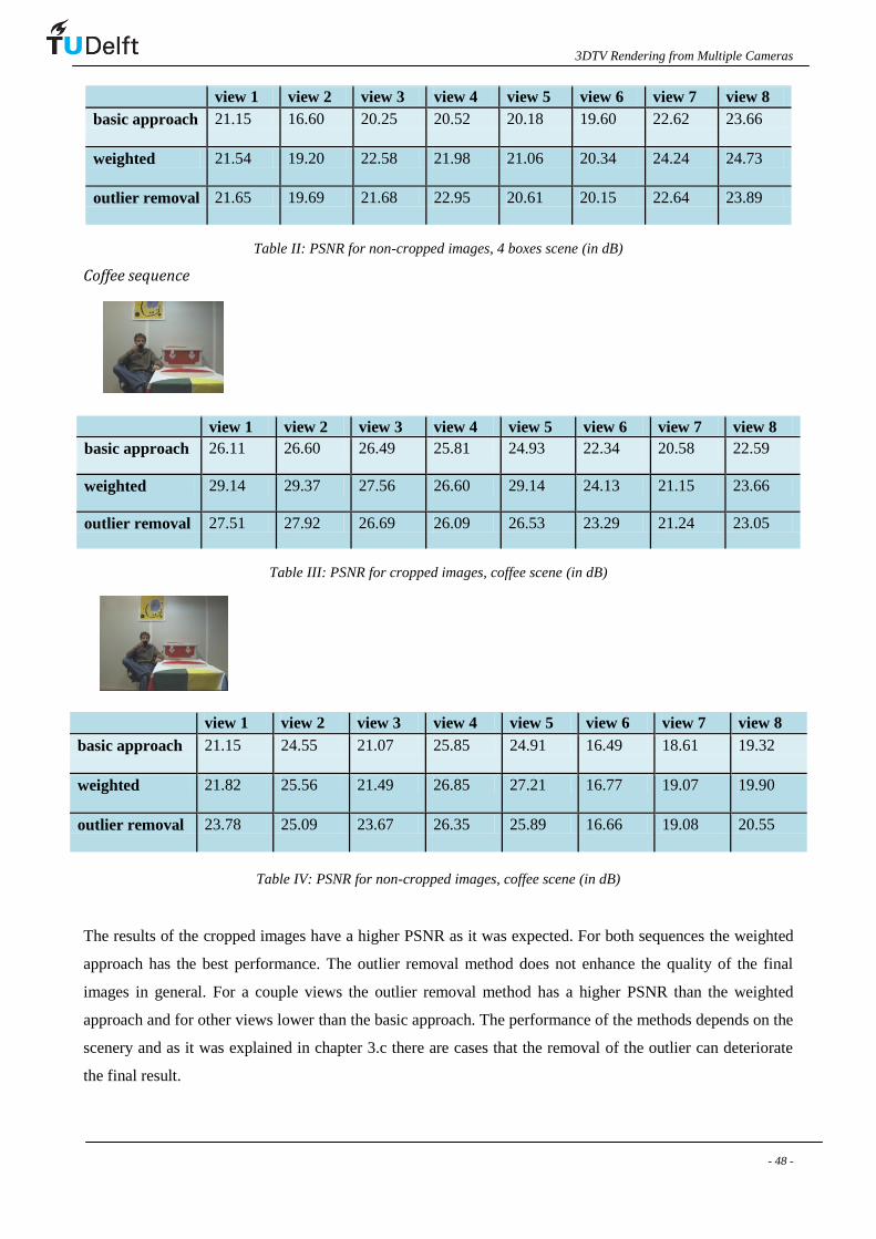
3DTV Rendering from Multiple Cameras
- 48 -
view 1 view 2 view 3 view 4 view 5 view 6 view 7 view 8
basic approach 21.15 16.60 20.25 20.52 20.18 19.60 22.62 23.66
weighted 21.54 19.20 22.58 21.98 21.06 20.34 24.24 24.73
outlier removal 21.65 19.69 21.68 22.95 20.61 20.15 22.64 23.89
Table II: PSNR for non-cropped images, 4 boxes scene (in dB)
Coffee sequence
view 1 view 2 view 3 view 4 view 5 view 6 view 7 view 8
basic approach 26.11 26.60 26.49 25.81 24.93 22.34 20.58 22.59
weighted 29.14 29.37 27.56 26.60 29.14 24.13 21.15 23.66
outlier removal 27.51 27.92 26.69 26.09 26.53 23.29 21.24 23.05
Table III: PSNR for cropped images, coffee scene (in dB)
view 1 view 2 view 3 view 4 view 5 view 6 view 7 view 8
basic approach 21.15 24.55 21.07 25.85 24.91 16.49 18.61 19.32
weighted 21.82 25.56 21.49 26.85 27.21 16.77 19.07 19.90
outlier removal 23.78 25.09 23.67 26.35 25.89 16.66 19.08 20.55
Table IV: PSNR for non-cropped images, coffee scene (in dB)
The results of the cropped images have a higher PSNR as it was expected. For both sequences the weighted
approach has the best performance. The outlier removal method does not enhance the quality of the final
images in general. For a couple views the outlier removal method has a higher PSNR than the weighted
approach and for other views lower than the basic approach. The performance of the methods depends on the
scenery and as it was explained in chapter 3.c there are cases that the removal of the outlier can deteriorate
the final result.

3DTV Rendering from Multiple Cameras
- 49 -
Another remark is that when the whole image is evaluated the outlier removal method has better metrics than
the basic and the weighted approach. The method handles better the generation of the borders of the images,
but this is not indicative of its general behaviour.
Yalazan et al.,[43] are proposing the derivative signal to noise ratio as an objective fidelity criterion
which considers the sensitivity of the human eye to the edge information. Human eye uses edge
information while perceiving an image. The authors claim that the new criterion should be sensitive
to regions of fast changes (edges) in an image in order to agree with subjective decisions.
ji
ro
ji
o
jiIjiI
jiI
SNRDerivative
,
2
,
2
10
)),(),((
),(log10
(20)
Where ),( jiIo and ),( jiI
r are approximate gradients at the (i,j)
th pixel of the original and
reconstructed images respectively, which are calculated as:
|)1,(),(||),1(),(|),( jiIjiIjiIjiIjiI (21)
The last row and last column are not used in the calculation of derivative SNR since the above
equation cannot be applied to those pixels. The equation computes the horizontal and vertical
changes at each pixel, hence the edge information is emphasized. In other words I(i,j) extracts the
high frequency components of the image. When a reconstruction process is not much successful in
reproducing the edges of the original image, the noise term in the denominator of the equation gets
large resulting in a poor value of the derivative SNR. The derivative SNR criterion which
emphasizes the contribution from the high frequency region is expected to be more correlated to
subjective decisions because of its similarity to the perceptional mechanism of the human eye.
4 boxes sequence
view 1 view 2 view 3 view 4 view 5 view 6 view 7 view 8
basic approach
(x10-5
)
0.26 0.19 0.12 0.19 0.14 0.18 0.24 0.25
weighted
(x10-5
)
0.27 0.19 0.14 0.20 0.15 0.17 0.24 0.25
outlier removal
(x10-5
)
0.18 0.10 0.10 0.14 0.11 0.11 0.13 0.15
Table V: Derivative SNR for cropped images, 4 boxes sequence (in dB)

3DTV Rendering from Multiple Cameras
- 50 -
Coffee sequence
view 1 view 2 view 3 view 4 view 5 view 6 view 7 view 8
basic approach
(x10-5
)
0.21 0.31 0.20 0.31 0.27 0.19 0.19 0.18
weighted
(x10-5
)
0.21 0.33 0.21 0.28 0.35 0.18 0.17 0.18
outlier removal
(x10-5
)
0.15 0.21 0.18 0.19 0.18 0.11 0.09 0.14
Table VI: Derivative SNR for cropped images, coffee sequence (in dB)
The values of the derivative SNR highlight the fact that the outlier removal method is the least visually
acceptable. As it is going to be discussed in the subjective evaluation, the outlier removal method gives non-
smoothed images and this irritates the visual perception.
In order to evaluate subjectively the methods, the results on Appendix A are used. The virtual views
regenerated from the basic approach are visually acceptable taking into account that the method remains
quite simple and fast. To have a better insight, the scene under consideration can be divided into different
parts. The borders of the images, where there are artifacts, should be excluded from the evaluation phase.
In the first scene, the background is highly textured. The background in the regenerated images keeps the
high texture. The white table is a homogeneous area at the original views except few pixels due to
illumination changes; in general the reconstructed table has a smooth view. The problem with this approach
is located in the area around the boxes and especially between the two boxes at the right (the purple and the
stripped one). Part of background that should be visible is erroneously reconstructed.
Figure 31: A virtual view generated by the basic approach.
When the camera proximity weights are integrated in the method the generated virtual views are better. The
improvement is visible especially for the last virtual views, where the occlusion problem is present.

3DTV Rendering from Multiple Cameras
- 51 -
Figure 32: A virtual view generated by the weighted approach.
The quality of the images generated by the outlier removal method seems to deteriorate in
comparison with the weighted approach. A grain effect is visible especially in homogeneous areas
like the table. The camera values are not averaged, some of them are not participating in the
calculation of the color of the pixel. This has as a consequence that the surfaces are less smooth.
The occlusions are handled well, and this was expected since the proximity weights are used as
well.
Figure 33: A virtual view generated by the outlier removal approach
The coffee sequence, has a smooth simple background, and does not include a highly occluded area.
The results for this sequence are visually better. The basic approach gives a bit blurred images, but
the other two methods seem to work efficiently.

3DTV Rendering from Multiple Cameras
- 52 -
6. Discussion and Future work
The goal of the research of this thesis was to study the feasibility of a simple algorithm to create 3D
content for 3DTV applications. The requirements of a 3DTV application for a whole scene video
with editing capabilities and high quality, and the constraints imposed by the number of the
available cameras formulate the research area.
First the state of the art methods were investigated. There are two main categories, as it was
discussed in detail in chapter two. The model-based approaches, using complex geometry models of
the scene. Synthetic videos, using blue-screen as a background for example, can be generated with
such techniques but their complexity makes their use prohibitive for the generation of a video of the
whole scene. The other category, image-based approaches, is able to reconstruct 3D videos for
whole scenes and that is that makes it more promising for 3DTV applications. The dense sampling
of the scene that is required complicates its use.
Current methods cannot work efficiently without imposing a lot of limitations. That was the
motivation of this thesis. We investigated a new approach that uses per-pixel operations to allow for
parallel computations, scalability and flexibility. For each pixel to be rendered a depth hypothesis
was generated. It was solved by projecting the pixel in the camera planes and comparing the color
values. The algorithm worked properly, with some exceptions, e.g. areas with occlusion. To
overcome the occlusion problem camera proximity weights were assigned to the cameras. The
distance between the position of the virtual and original camera was calculated. Original cameras
closer to the camera view were assigned a greater weight. The improvement in the visual quality of
the generated images was significant.
However artifacts were still present. Investigation of the RGB values of the eight cameras for one
pixel, indicated that there were different reasons for which the camera agreement hypothesis for the
correct depth was not true. An occlusion for example is a potential cause for outlier values in the
RGB dataset. To solve the outlier problem we investigated two approaches, a non-weighted outlier
removal and a weighted outlier removal method. The generated images are not visually better in
comparison with the ones generated with the basic approach. However for some special areas the
outlier removal method works properly. So, integration of more sophisticated criterions in the depth
selection stage may lead to better results.

3DTV Rendering from Multiple Cameras
- 53 -
The methods discussed have the advantage that can generate a 3D video of the whole scene while
they keep the computational complexity of the system low and have as input only eight original
images. They can directly benefit by using more cameras or cameras with higher resolution in order
to enhance the final result.
The fact that there is no intermediate representation, adds on the freedom of the adopted methods
but on the other hand any inter-view relations are not taken into account. Every time a new virtual
view is generated the analysis stage has to run.
To sum up, after analyzing in detail the behavior of pixels in the reconstruction stage we gained a
very good insight of their behavior. This information was incorporated in the approaches tested. The
results are very promising. Some improvements can be made. The scenery for example can be
segmented in areas according to their special characteristics (e.g. occluded areas, objects at the
front). Then each segment could be regenerated by a different approach according to its special
characteristics. The depth maps of the generated images, (Appendix C) could be used as an
indicator of which areas need special attention. In Appendix B, a clustering experiment highlights
the fact that the special characteristics within an area of the image are spatial consistent.
b. Future Research
Layered Depth Images are used widely for rendering 3D objects. Our approach could be extended
to more than one layer. The per-pixel analysis facilitates the generation of layers from the original
images. Preliminary experiments were conducted in which the layers were selected as modes of the
color variance. The depth with minimum color variance was considered as the first layer, the depth
with the second minimum variance the second one.
The spatial and temporal connectivity, both present in sequence of images, were not taken into
account. In a future research their use could enhance for example the non-smooth result of the
outlier removal method.

3DTV Rendering from Multiple Cameras
- 54 -
7. Appendix
A. Results
Four boxes sequence
Figure 34: Six of the virtual views for the 4 boxes sequence generated with the basic approach. The positions if the
virtual cameras are shown in figure 40.

3DTV Rendering from Multiple Cameras
- 55 -
Figure 35: Six of the virtual views for the 4 boxes sequence generated with the weighted approach.

3DTV Rendering from Multiple Cameras
- 56 -
Figure 36: Six of the virtual views for the 4 boxes sequence generated with the outlier removal approach.

3DTV Rendering from Multiple Cameras
- 57 -
coffee sequence
Figure 37: Six of the virtual views for the coffee sequence generated with the basic approach.

3DTV Rendering from Multiple Cameras
- 58 -
Figure 38: Six of the virtual views for the coffee sequence generated with the weighted approach.

3DTV Rendering from Multiple Cameras
- 59 -
Figure 39: Six of the virtual views for the coffee sequence generated with the outlier removal approach.
Figure 40: The red stars are indicating the positions of the six virtual views shown in the previous figures, in relevance
to the original cameras configuration.

3DTV Rendering from Multiple Cameras
- 60 -
B . Clustering experiment
Here, a pixel is considered, and the outlier removal algorithm is iterated eight times, having as a starting
point, Vc, one of the vectors containing the RGB information for one of the cameras each time. The dataset
of the algorithm are the eight Vc vectors. For the different iteration points the algorithm outputs different
mean values.
Then the eight different mean values are compared, and values with distance less than a threshold are
combined. In this way the possibility of different clusters or single outlier values within the dataset of the
eight Vc vectors is investigated. The purpose of this experiment is to test in areas with different
characteristics what camera clusters are generated for different depths. The spatial consistency of these
results is also investigated.
In the following diagram, one pixel in the front part of the four boxes sequence is considered, and the clusters
found for every depth are visualized. The blue line is the variance of all the eight cameras as a function of
depth calculated with the basic approach as discussed in section 3.a. The „x‟ represents one cluster, its y
value indicates the variance of the cluster and finally the color stands for the number of the cameras
participating in the cluster. This figure corresponds to one pixel in the front part of the image, on the table. It
can be noticed easily that for the correct depth, around 1.4 meters, all the eight cameras are in agreement.
Therefore there are no outliers.
1
2
3
Figure 41: Position of the three pixels discussed in this section

3DTV Rendering from Multiple Cameras
- 61 -
1 1.5 2 2.5 30
5000
10000
15000
Depth
Col
or V
aria
nce
Depth-variance plot
1 cam
2 cams
3 cams
4 cams
5 cams
6 cams
7 cams
8 cams
Figure 42: Depth –color variance plot. The „x‟ symbol stands for a cluster of cameras. Its color indicates the number of
the members of the cluster, its height the variance of the cluster. For a pixel in the front part of the image (Figure 20),
all the eight cameras are in agreement for the correct depth.
To check the consistency of the clustering between neighboring pixels, the clustering algorithm now is
performed in more pixels, sequential in the x axis. Only the biggest cluster of each depth is plotted in the
next diagram.
1 1.5 2 2.5 30
10
20
30
40
50
60
Depth
x ax
is
1 cam
2 cams
3 cams
4 cams
5 cams
6 cams
7 cams
8 cams
Figure 43: The number of camera members of a cluster is indicated by the color of the x symbol. 40 pixels successive in
the x axis are considered.
A pixel in the occluded area is now considered. The created clusters comprise of 1-3 cameras highlighting
the fact that the cameras are distracted by occlusion. The same holds for neighboring pixels.

3DTV Rendering from Multiple Cameras
- 62 -
1 1.5 2 2.5 30
1000
2000
3000
4000
5000
6000
7000
8000
9000
10000
Depth
Col
or V
aria
nce
Depth-variance plot
1 cam
2 cams
3 cams
4 cams
5 cams
6 cams
7 cams
8 cams
Figure 44: Depth –color variance plot. The „x‟ symbol stands for a cluster of cameras. Its color indicates the number of
the members of the cluster, its height the variance of the cluster. For a pixel in the occlusion area (Figure 27), the
cameras are not in agreement and they are forming separated small clusters.
1 1.5 2 2.5 30
5
10
15
20
25
30
35
40
45
Depth
y ax
is
1 cam
2 cams
3 cams
4 cams
5 cams
6 cams
7 cams
8 cams
Figure 45: The number of camera members of a cluster is indicated by the color of the x symbol. 40 pixels successive in
the y axis are considered.
A pixel in the box positioned in the middle of the table is considered. The cameras are in agreement but for a
wide range of depths (Figure 46).
The clustering is performed for neighboring pixels, in both axis x and y (Figures 47 and 48). It can be
noticed that within this neighborhood of pixels, the number of camera members is consistent for similar
depths.

3DTV Rendering from Multiple Cameras
- 63 -
1 1.5 2 2.5 30
2000
4000
6000
8000
10000
12000
Depth
Col
or V
aria
nce
Depth-variance plot
1 cam
2 cams
3 cams
4 cams
5 cams
6 cams
7 cams
8 cams
Figure 46: Depth –color variance plot. The „x‟ symbol stand for a cluster of cameras. Its color indicates the number of
the members of the cluster, its height the variance of the cluster. For a pixel on the box, the cameras are in agreement
for a wide area of depths.
1 1.5 2 2.5 30
5
10
15
20
25
30
35
40
45
Depth
y ax
is
1 cam
2 cams
3 cams
4 cams
5 cams
6 cams
7 cams
8 cams
Figure 47: The number of camera members of a cluster is indicated by the color of the x symbol. 40 pixels successive in
the y axis are considered.

3DTV Rendering from Multiple Cameras
- 64 -
1 1.5 2 2.5 30
5
10
15
20
25
30
35
40
45
Depth
x ax
is
1 cam
2 cams
3 cams
4 cams
5 cams
6 cams
7 cams
8 cams
Figure 48: The number of camera members of a cluster is indicated by the color of the x symbol. 40 pixels successive in
the x axis are considered.
C. Depth maps
Our approach when reconstructing a virtual view is implicitly reconstructing its depth map. Three
depth maps are shown here reconstructed by the basic, the weighted and the outlier removal
approach respectively.
Figure 49: virtual view and its depth map reconstructed with the basic approach.
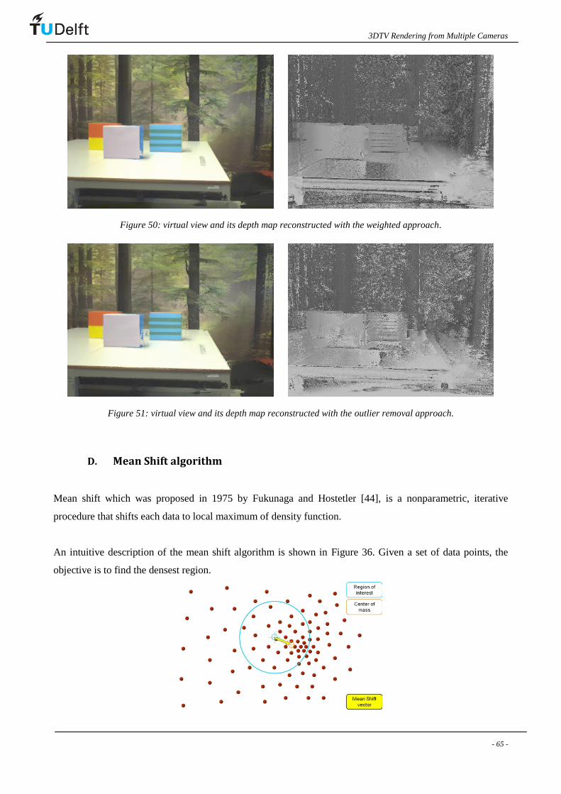
3DTV Rendering from Multiple Cameras
- 65 -
Figure 50: virtual view and its depth map reconstructed with the weighted approach.
Figure 51: virtual view and its depth map reconstructed with the outlier removal approach.
D. Mean Shift algorithm
Mean shift which was proposed in 1975 by Fukunaga and Hostetler [44], is a nonparametric, iterative
procedure that shifts each data to local maximum of density function.
An intuitive description of the mean shift algorithm is shown in Figure 36. Given a set of data points, the
objective is to find the densest region.

3DTV Rendering from Multiple Cameras
- 66 -
Figure 40: Intuitive description of mean shift algorithm. In the above distribution of identical billiard balls, the
objective is to find the densest region.
The mean shift algorithm does not require prior knowledge of the number of clusters, and does not constraint
the shape of clusters.
Given { xi }i = 1,…n an arbitrary set of n points in the d-dimensional Euclidean space Rd. The multivariate
kernel density estimate obtained with kernel K(x) and a symmetric positive, dd ,bandwidth matrix H,
computed in the point x is given by,(22):
n
i
iHxxK
nxf
1
1)(ˆ
(22)
where
xHKHxKH
2/12/1
)(
(23)
The d-variate kernel K(x) is a bounded function satisfying:
dR
dxxK 1)(
0)(lim
xKxd
x
d
R
dxxxK 0)( d
R
K
TIcdxxKxx )(
(24)
where cK is a constant.
A special class of radially symmetric kernels satisfying:
)()(2
,xkcxK
dk
(25)
is of interest in the work of Comaniciu et al.,[45], where k(.) is called the profile of the kernel and ck,d is a
normalization constant.
Employing a fully parameterized H increases the complexity of the estimation. Employing only one
bandwidth parameter, the kernel density estimator (1) becomes:
n
i
i
dh
xxK
nhxf
1
1)(ˆ
(26)
Employing the profile notation, the density estimator (26) can be rewritten as:
n
i
i
d
dk
Khh
xxk
nh
cxf
1
2
,
,)(ˆ (27)

3DTV Rendering from Multiple Cameras
- 67 -
The first step in the analysis of a space with the underlying density f(x) is to find the modes of this density.
The modes are located among the zeros of the gradient 0)( xf and the mean shift procedure is an way to
locate these zeros without estimating the density.
The density gradient estimator obtained as the gradient of the density estimator:
2
1
2
,
,,)(
2)(ˆ)(ˆ
h
xxkxx
nh
cxfxf
i
n
i
id
dk
KhKh (28)
The function )()( xkxg is defined, assuming that the derivative of the kernel profile exists for all
x ,0 , except for a finite set of points. Using g(x) for profile, the kernel G(x) is defined as:
2
,)( xgcxG
dg
(29)
Where ck,d is the corresponding normalization constant. The kernel K(x) was called the shadow of G(x). The
Epanechnikov kernel is the shadow of the uniform kernel, while the normal kernel and its shadow have the
same expression.
Introducing g(x) into (28), yields
x
h
xxg
h
xxgx
h
xxg
nh
c
h
xxgxx
nh
cxf
n
i
i
n
i
i
in
i
i
d
dkn
i
i
id
dk
Kh
1
2
1
2
1
2
2
,
1
2
2
,
,
22)(ˆ (30)
where
n
i
i
h
xxg
1
2
is assumed to be a positive number. This condition is easy to satisfy for all the
profiles met in practice. Both terms of the product in (30) have special significance. From (27), the first term
is proportional to the density estimate at x computed with the kernel G.
n
i
i
d
dk
Khh
xxg
nh
cxf
1
2
,
,)(ˆ (31)
The second term is the mean shift

3DTV Rendering from Multiple Cameras
- 68 -
x
h
xxg
h
xxgx
xmn
i
i
n
i
i
i
Gh
1
2
1
2
,)( (32)
i.e. the difference between the weighted mean, using the kernel G for weights, and x, the center of the
kernel(window). From (31) and (32), (30) becomes
)(2
)(ˆ)(ˆ,2
,
,,xm
nh
cxfxf
Ghd
dk
GhKh
(33)
yielding
)(ˆ
)(ˆ
2
1)(
,
,2
,
xf
xfchxm
Gh
Kh
Gh
(34)
The expression (34) shows that, at location x, the mean shift vector computed with kernel G is proportional
to the normalized density gradient estimate obtained with kernel K. The normalization is by the density
estimate in x computed with the kernel G.
The relation captured in (34) is intuitive; the local mean is shifted toward the region in which the majority of
the points reside. Since the mean shift vector is aligned with the local gradient estimate, it can define a path
leading to a stationary point of the estimated density. The modes of the density are such stationary points.
The mean shift procedure, obtained by successive
Computation of the mean shift vector )(,
xmGh
Translation of the kernel (window) G(x) by )(,
xmGh
will converge at a nearby point where the estimate has zero gradient.

3DTV Rendering from Multiple Cameras
- 69 -
8. References
[1] W.Matusik, H. Pfister, 3D TV: a scalable system for real-time acquisition, transmission, and
autostereoscopic display of dynamic scenes, International Conference on Computer Graphics and Interactive
Techniques archive ACM SIGGRAPH 2004
[2] A.Kubota, A. Smolic, M. Magnor, M. Tanimoto, Ts. Chen, Ch. Zhang, Multiview Imaging and 3DTV,
Signal Processing Magazine IEEE, v.24, issue(6), 2007
[3] Wilburn, B., N. Joshi, V. Vaish, E.-V. Talvala, E. Antunez, A. Barth, A. Adams, M. Horowitz, and M.
Levoy: 2005, High performance imaging using large camera arrays, Proceedings of SIGGRAPH (ACM
Transactions on Graphics) 24(3), 765–776.
[4] Zitnick, C. L., S. B. Kang, M. Uyttendaele, S.Winder, R. Szeliski, High-quality video view interpolation
using a layered representation, Proceedings of SIGGRAPH (ACM Transactions on Graphics) 2004, pp.
600–608.
[5] Kanade, T., P. W. Rander, P. J. Narayanan: 1997, Virtualized Reality: Constructing virtual worlds from
real scenes, IEEE MultiMedia Magazine 1(1), 34–47.
[6] L.Onural, Th.Sikora, J.Ostermann, A.Smolic, M.R.Civanlar, J.Watson, An Assessment of 3DTV
Technoloigies, 2006 NAB BEC Proceedings
[7] M. op den Beeck, A. Redert, Three dimensional video for the home, Proceedings of EUROIMAGE
ICAV3D 2001, International Conference on Augmented, Virtual Environments and Three-
Dimensional Imaging, Mykonos, Greece, May 30 – June 1, 2001, pp. 188-191
[8] R. Börner, B. Duckstein, O. Machui, R. Röder, T. Sinning and T. Sikora, A family of single-user
autostereoscopic displays with head-tracking capabilities, IEEE Transactions on Circuits and Systems for
Video Technology, Vol. 10, No. 2, pp. 234- 243, 2000
[9] Philips lenticular screens, http:// www.research.philips.com/generalinfo/special/3dlcd
[10] J. Carranza, C. Theobalt, M. Magnor, H.-P. Seidel, Free-viewpoint video of human actors, in Proc.
ACM Conf. Comput. Graph. (SIGGRAPH‟03), 2003, pp. 569–577.

3DTV Rendering from Multiple Cameras
- 70 -
[11] C. Theobalt, N. Ahmed, G. Ziegler, H. Seidel, High-Quality Reconstruction from Multiview Video
Streams, Dynamic representation of 3-D human actors, Signal Processing Magazine IEEE, v.24, issue(6),
2007
[12] T. Matsuyama, X. Wu, T. Takai, T. Wada, Real-Time Dynamic 3-D Object Shape Reconstruction and
High-Fidelity Texture Mapping for 3-D Video, IEEE Transactions on Circuits and Systems for Video
Technology, vol.14, no.3, March 204.
[13] S. Vedula, S. Baker, T. Kanade, Spatio-temporal view interpolation, In: EGRW '02, pp. 65.76, 2002
[14] T. Fujii, T. Kimoto, M. Tanimoto, Ray space coding for 3D visual communication, Picture Coding
Symp. 1996, Mar. 1996, pp. 447–451.
[15] M. Levoy, P. Hanrahan, Light field rendering, in Proc. ACM SIGGRAPH, Aug. 1996, pp. 31–42.
[16] H.Y. Shum, L.W. He, Rendering with concentric mosaics, in Proc. ACM SIGGRAPH, Aug. 1999, pp.
299–306.
[17] E.H. Adelson, J.R. Bergen, The plenoptic function and the elements of early vision, In Computational
Models of Visual Processing, Landy and Movshon, Eds. MIT Press, Cambridge, Massachusetts, 1991, ch. 1.
[18] L. McMillan and G. Bishop, Plenoptic modeling: an image-based rendering system, in Proc. Comput.
Graphics (SIGGRAPH ‟95), 1995, pp. 39–46.
[19] S.J. Gortler, R. Grzesczuk, R. Szeliski, and M.F. Cohen, The Lumigraph, in Proc. ACM
SIGGRAPH‟96, Aug. 1996, pp. 43–54
[20] C. Fehn, P. Kauff, M. Op de Beeck, F. Ernst, W. Ijsselsteijn, M. Pollefeys, L. Vangool, E. Ofek, I.
Sexton, An evolutionary and optimised approach on 3DTV, IBC 2002, Int. Broadcast Convention,
Amsterdam, Netherlands, Sept. 2002
[21] P. Debevec, C. Taylor, J. Malik, Modeling and rendering architecture from photographs: A hybrid
geometry- and image-based approach, in Proc. SIGGRAPH 1996, 1996, pp. 11–20.
[22] S. Wurmlin, E. Lamboray, M. Gross, 3D video fragments: Dynamic point samples for real-time free-
viewpoint video, Comput. Graph., (Special issue on coding, compression and streaming techniques for 3D
and multimedia data), vol.28, no. 1, pp. 3–14, 2004.
3DTV Rendering from Multiple Cameras
- 71 -
[23] M. Waschbusch, St.Wurmlin, D. Cotting, F. Sadlo, M. Gross, Scalable 3D Video of Dynamic Scenes,
the Visual Computer 21(8-10):629-638, 2005
[24] A. Broadhurst, T. Drummond, R. Cipolla, A probabilistic framework for the space carving algorithm,
In: ICCV '01, pp. 388.393 (2001)
[25] http://graphics.ethz.ch/research/3dvideo/
[26] J. Shade, S. Gortler, L. Hey, and R. Szeliski, “Layered depth images,” in Proceedings of ACM
SIGGRAPH‟98, Orlando, Florida, 1998, pp. 231–242.
[27] S. M. Seitz, C. R. Dyer, Photorealistic scene reconstruction by voxel coloring, in Proceedings of
Conference on Computer Vision and Pattern Recognition, 1997, pp. 1067–1073.
[28] Y. Chuang, A Bayesian Approach to Digital Matting, In Conference on Computer Vision and Pettern
Recognition (CVPR), vol.11, 264-271, 2001.
[29] Dongbo Min Donghyun Kim Kwanghoon Sohn , Virtual View Rendering System for 3DTV, 3DTV
Conference: The True Vision - Capture, Transmission and Display of 3D Video, 2008
[30] A. Smolić, K. Mueller, P. Merkle, T. Rein, M. Kautzner, P. Eisert, and T. Wiegand, Representation,
coding, and rendering of 3D video objects with MPEG-4 and H.264/AVC, Multimedia Signal Processing,
2004 IEEE 6th Workshop on, 29 Sept.-1 Oct. 2004, p. 379- 382
[31] Martin A. Fischler and Robert C. Bolles (June 1981), Random Sample Consensus: A Paradigm for
Model Fitting with Applications to Image Analysis and Automated Cartography, Comm. of the ACM 24:
381–395
[32] C. Yang, R. Duraiswami, D. DeMenthon and L. Davis. Mean-Shift Analysis Using Quasi-Newton
Methods, In IEEE International Conference on Image Processing, pages 447 - 450, vol.3, 2003.
[33] P.A. Redert (J. Biemond and E.A. Hendriks thesis advisors), Multi-Viewpoint Systems for 3D
Visual Communication, Ph.D. thesis, ISBN 90-901-3985-0, pp. 241, October 2000.
[34] A. M. Eskicioglu, Application of multidimensional quality measures to reconstructed medical images,
Opt. Eng. 35(3), 778–785 (1996).
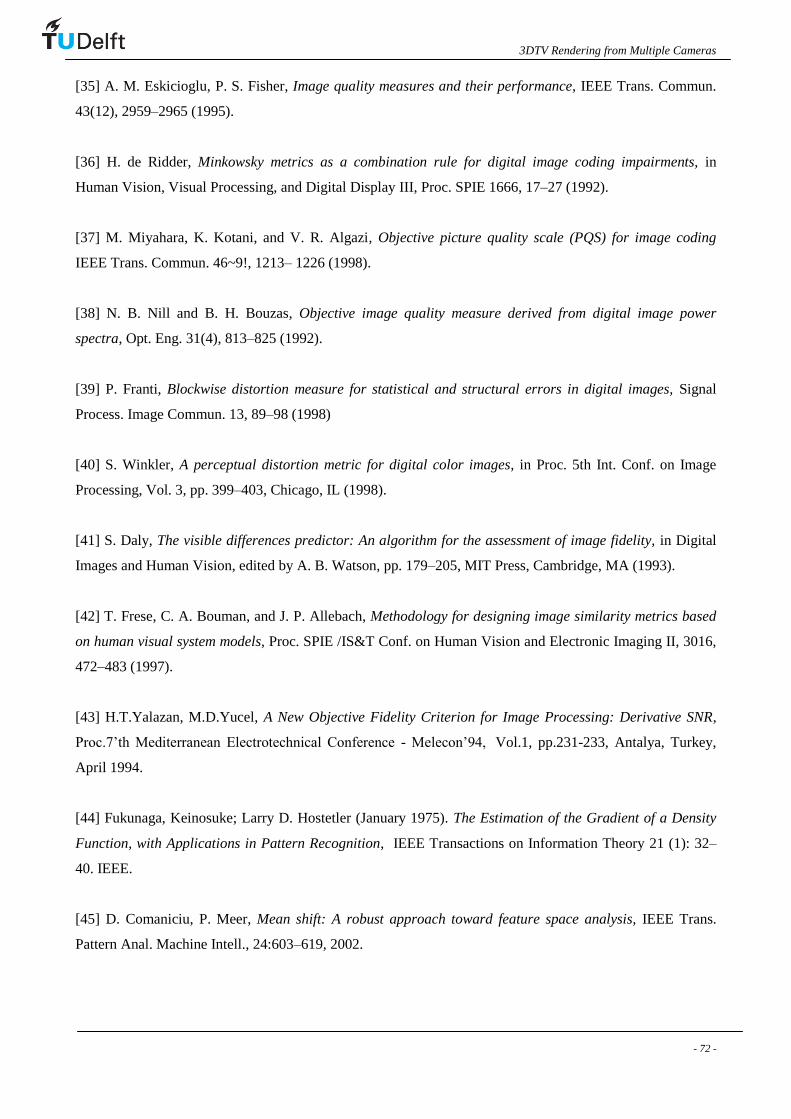
3DTV Rendering from Multiple Cameras
- 72 -
[35] A. M. Eskicioglu, P. S. Fisher, Image quality measures and their performance, IEEE Trans. Commun.
43(12), 2959–2965 (1995).
[36] H. de Ridder, Minkowsky metrics as a combination rule for digital image coding impairments, in
Human Vision, Visual Processing, and Digital Display III, Proc. SPIE 1666, 17–27 (1992).
[37] M. Miyahara, K. Kotani, and V. R. Algazi, Objective picture quality scale (PQS) for image coding
IEEE Trans. Commun. 46~9!, 1213– 1226 (1998).
[38] N. B. Nill and B. H. Bouzas, Objective image quality measure derived from digital image power
spectra, Opt. Eng. 31(4), 813–825 (1992).
[39] P. Franti, Blockwise distortion measure for statistical and structural errors in digital images, Signal
Process. Image Commun. 13, 89–98 (1998)
[40] S. Winkler, A perceptual distortion metric for digital color images, in Proc. 5th Int. Conf. on Image
Processing, Vol. 3, pp. 399–403, Chicago, IL (1998).
[41] S. Daly, The visible differences predictor: An algorithm for the assessment of image fidelity, in Digital
Images and Human Vision, edited by A. B. Watson, pp. 179–205, MIT Press, Cambridge, MA (1993).
[42] T. Frese, C. A. Bouman, and J. P. Allebach, Methodology for designing image similarity metrics based
on human visual system models, Proc. SPIE /IS&T Conf. on Human Vision and Electronic Imaging II, 3016,
472–483 (1997).
[43] H.T.Yalazan, M.D.Yucel, A New Objective Fidelity Criterion for Image Processing: Derivative SNR,
Proc.7‟th Mediterranean Electrotechnical Conference - Melecon‟94, Vol.1, pp.231-233, Antalya, Turkey,
April 1994.
[44] Fukunaga, Keinosuke; Larry D. Hostetler (January 1975). The Estimation of the Gradient of a Density
Function, with Applications in Pattern Recognition, IEEE Transactions on Information Theory 21 (1): 32–
40. IEEE.
[45] D. Comaniciu, P. Meer, Mean shift: A robust approach toward feature space analysis, IEEE Trans.
Pattern Anal. Machine Intell., 24:603–619, 2002.