RECENT ADVANCES IN HAPTIC RENDERING AND ...
312
RECENT ADVANCES IN HAPTIC RENDERING AND APPLICATIONS Edited by Ming C. Lin and Miguel A. Otaduy Copyright © 2005 1
-
Upload
khangminh22 -
Category
Documents
-
view
0 -
download
0
Transcript of RECENT ADVANCES IN HAPTIC RENDERING AND ...

RECENT ADVANCES IN HAPTIC RENDERING AND
APPLICATIONS
Edited by Ming C. Lin and Miguel A. Otaduy
Copyright © 2005
1

2

ORGANIZERS Ming C. Lin Department of Computer Science University of North Carolina Chapel Hill, NC 27599-3175 [email protected] PHO: 919-962-1974 FAX: 919-962-1799 Miguel Otaduy Department of Computer Science Institute of Scientific Computing ETH Zentrum CH - 8092 Zürich [email protected]
3

LECTURERS • Elaine Cohen, University of Utah [email protected] • David Johnson, University of Utah [email protected] • Roberta Klatzky, Carnegie Mellon University
[email protected] • Ming Lin, University of North Carolina at Chapel Hill
[email protected] • Bill McNeely, Boeing Research [email protected] • Miguel Otaduy, ETH Zurich
[email protected] • Dinesh Pai, Rutgers University [email protected] • Ken Salisbury, Stanford University & Intuitive Surgery, Inc [email protected] • Hong Tan, Purdue University [email protected]
• Russell Taylor, University of North Carolina at Chapel Hill
4

BIOGRAPHICAL SKETCHES OF LECTURERS Elaine Cohen is a professor of computer science at the University of Utah. She is co-head of the Geometric Design and Computation Project and co-author of Geometric Modeling with Splines: An Introduction (A. K. Peters, 2001). Dr. Cohen has focused her research in computer graphics, geometric modeling, and manufacturing, with emphasis on complex sculptured models represented using NURBS (Non-Uniform Rational B-splines) and NURBS-features. Results in manufacturing research have been focused on automating process planning, automatic toolpath generation for models having many surfaces, optimizing both within and across manufacturing stages and fixture automation. She has also been working on issues related to telepresence and design collaborations in virtual environments. Recent research has produced algorithms for determining both visibility and accessibility of one object by another. Computation of such information is necessary for manufacturing, assembly planning, graphics, and virtual environments. Research in haptics has been focused on developing new approaches to solving geometric computations such as fast and accurate contact and tracking algorithms for sculptured models and while research in haptics systems has focused on realistic force feedback in distributed haptic systems for complex mechanical models. Dr. Cohen was the 2001 recipient of the University of Utah Distinguished Research Award and is a member of the Computer Science and Telecommunications Board of the National Academies. Website: http://www.cs.utah.edu/~cohen/ David Johnson is a research scientist at the University of Utah, School of Computing, where he also received his PhD. His primary research interest is in distance algorithms for haptic rendering, motivated by the needs of virtual prototyping applications. He has given invited talks at Ford Motor Company, Intel Research, and Institute for Mathematics and its Applications on these topics. In addition, he was a speaker at a Solid Modeling 2001 tutorial on haptic rendering. Website: http://www.cs.utah.edu/~dejohnso/ Roberta Klatzky is a Professor of Psychology at Carnegie Mellon University, where she also holds faculty appointments in the Center for the Neural Basis of Cognition and the Human-Computer Interaction Institute. She served as Head of Psychology from 1993 - 2003. She received a B.S. in mathematics from the University of Michigan and a Ph.D. in experimental psychology from Stanford University. Klatzky's research interests are in human perception and cognition, with special emphasis on haptic perception and spatial cognition. She has done extensive research on haptic and visual object recognition, human navigation
5

under visual and nonvisual guidance, and motor planning. Her work has application to haptic interfaces, navigation aids for the blind, exploratory robotics, teleoperation, and virtual environments. She also has interests in medical decision-making. Professor Klatzky is the author of over 150 articles and chapters, and she has authored or edited 4 books. Klatzky has been a member of the National Research Council's Committee on Human Factors and Committee on Techniques for Enhancing Human Performance, as well as other working groups of the NRC. Her service to scientific societies includes chairing the governing board of the Psychonomics Society and the Psychology Section of AAAS, as well as serving as Treasurer of the American Psychological Society and being on the advisory board of the International Association for the Study of Attention and Performance. She is a member of several editorial boards and a past associate editor of the journal Memory and Cognition.
Website: http://www.psy.cmu.edu/faculty/klatzky/
Ming Lin received her B.S., M.S., Ph.D. degrees in Electrical Engineering and Computer Science all from the University of California, Berkeley. She is currently a full professor in the Computer Science Department at the University of North Carolina (UNC), Chapel Hill. She received the NSF Young Faculty Career Award in 1995, Honda Research Initiation Award in 1997, UNC/IBM Junior Faculty Development Award in 1999, and UNC Hettleman Award for Scholarly Achievements in 2002. Her research interests include haptics, physically-based modeling, robotics, and geometric computing. She has served as a program committee member for many leading conferences on virtual reality, computer graphics, robotics and computational geometry. She was the general chair and/or the program chair of the First ACM Workshop on Applied Computational Geometry, 1999 ACM Symposium on Solid Modeling and Applications, the Workshop on Intelligent Human Augementation and Virtual Environments 2002, ACM SIGGRAPH/EG Symposium on Computer Animation 2003, and ACM Workshop on General-Purpose Computing on GPUs 2004, Computer Animation and Social Agents 2005, and Eurographics 2005. She also serves on the Steering Committee of ACM SIGGRAPH/EG Symposium on Computer Animation. She is an associated editor and a guest editor of several journals and magazines, including IEEE Transactions on Visualization and Computer Graphics, International Journal on Computational Geometry and Applications, IEEE Computer Graphics and Applications, and ACM Computing Reviews. She also edited the book "Applied Computation Geometry.” She has given several lectures and invited presentations at SIGGRAPH, GDC, and many other international conferences. Website: http://www.cs.unc.edu/~lin/ and http://gamma.cs.unc.edu/
6

Bill McNeely obtained a Ph.D. in physics from Caltech in 1971 and for the next 6 years pursued physics research in Hamburg, Germany. In 1977 he began working for Boeing Computer Services in Seattle, Washington, developing advanced computer graphics for engineering applications. From 1981 to 1988 he served as chief engineer at startup company TriVector Inc., creating software products for technical illustration. In 1988 he founded the software consulting company McNeely & Associates. In 1989 he returned to Boeing, where he now holds the position of Technical Fellow. At Boeing he has pursued research in high-performance computer graphics, haptic simulation, and information assurance. Website: http://www.boeing.com/phantom/ Miguel Otaduy received his PhD in Computer Science in 2004 from the University of North Carolina, Chapel Hill, supported by fellowships from the Government of the Basque Country and UNC Computer Science Alumni. He received a bachelor’s degree in electrical engineering from University of Mondragon (Spain) in 2000. Between 1995 and 2000, he was a research assistant at the research lab Ikerlan. In the summer of 2003 he worked at Immersion Medical. His research areas include haptic rendering, physically-based simulation, collision detection, and geometric modeling. He and Lin introduced the novel concept of sensation preserving simplification for haptic rendering in their SIGGRAPH 2003 paper and proposed the first 6-DOF haptic texture rendering algorithm. He is currently a research associate at ETH Zurich. Website: http://graphics.ethz.ch/~otmiguel/ Dinesh Pai is a Professor in the Department of Computer Science at Rutgers University. Previously, he was a Professor at the University of British Columbia and a fellow of the BC Advanced Systems Institute. He received his Ph.D. from Cornell University. His research spans the areas of graphics, robotics, and human-computer interaction. His current work is in Human Simulation and Multisensory Computation; the latter includes multisensory simulation (integrating graphics, haptics, and auditory displays) and multisensory modeling (based on measurement of shape, motion, reflectance, sounds, and contact forces). He is the author of over 85 refereed publications, including 25 journal papers and 4 SIGGRAPH papers. He has served on 6 editorial boards and on the program committees of all major conferences in Robotics and Graphics, and is a program chair for the 2004 Symposium on Computer Animation. He organized the SIGGRAPH2001 Panel “Newton's Nightmare: Reality meets Faux Physics,” and co-taught the SIGGRAPH 2003 course on “Physics-Based Sound Synthesis for Graphics and Interactive Systems.” Website: http://www.cs.rutgers.edu/~dpai/
7

Kenneth Salisbury is well known for his seminal contributions to the fields of robotics, haptics, and robotically assisted surgery, and for his successes in facilitating transfer of these technologies. Professor Salisbury received his Ph.D. in Mechanical Engineering from Stanford University in 1982. From 1982 to 1999 he served at MIT as Principal Research Scientist in Mechanical Engineering and as a member of the Artificial Intelligence Laboratory. Among the projects with which he has been associated are the Stanford-JPL Robot Hand, the JPL Force Reflecting Hand Controller, the MIT-WAM arm, and the Black Falcon Surgical Robot. His work with haptic interface technology led to the founding of SensAble Technologies Inc., producers of the PHANTOM haptic interface and FreeForm software. In 1997 he became the Scientific Adviser to Intuitive Surgical in Mountain View, where his efforts focused on the development of dexterity-enhancing telerobotic systems for surgeons. In the Fall of 1999, he joined the faculty at Stanford in the departments of Computer Science and Surgery, where his research now focuses on human-centered robotics, collaborative computer-mediated haptics, and surgical simulation. He currently serves on the National Science Foundation's Advisory Council for Robotics and Human Augmentation, as Scientific Adviser to Intuitive Surgical, Inc., and as Technical Adviser to Robotic Ventures, Inc. Website: http://www.robotics.stanford.edu/~jks/ Hong Tan is founder and director of the Haptic Interface Research Laboratory at Purdue University. In 1986, she received a Bachelor's degree in Biomedical Engineering (with a minor in Computer Science) from Shanghai Jiao Tong University. She earned her Master and Doctorate degrees, both in Electrical Engineering and Computer Science, from the Massachusetts Institute of Technology (MIT) in 1988 and 1996, respectively. From 1991 to 1993, she was a Research Associate at the Tufts University School of Medicine. From 1996 to 1998, she was a Research Scientist at the MIT Media Laboratory. In 1998, she joined the faculty at Purdue's School of Electrical and Computer Engineering as an Assistant Professor, and in 2003 received tenure and promotion to an Associate Professor. Since 2002, she has held a courtesy appointment at Purdue's School of Mechanical Engineering for her contribution to the Perception-Based Engineering program. Her broad research interests in the area of haptic interfaces include psychophysics, haptic rendering, and distributed contact sensing. She is a recipient of National Science Foundation's Early Faculty Development (CAREER) Award (2000-2004). She has served on numerous conference program committees, and is currently co-organizer (with Blake Hannaford) of International Symposium on Haptic Interfaces for Virtual Environment and Teleoperator Systems (2003-2005). Website: http://www.ece.purdue.edu/~hongtan/
8

Russell Taylor is a Research Associate Professor of Computer Science, Physics & Astronomy, and Materials Science at the University of North Carolina at Chapel Hill. He has spent his 10-year career building scientific visualizations and interactive computer-graphics applications to help scientists better understand their instrumentation and data. He was the Principal Investigator on UNC's NIH National Research Resource on Computer Graphics for Molecular Studies and Microscopy and is now Co-director of UNC's NanoScale Science Research Group (www.cs.unc.edu/Research/nano). For the past two years, Russ has taught a "Visualization in the Sciences" course to computer science, physics, chemistry, statistics, and materials science graduate students. The course is based in large part on the textbook “Information Visualization: Perception for Design” (www.cs.unc.edu/Courses/comp290-069). Dr. Taylor has been a contributor to several past SIGGRAPH courses. Website: http://www.cs.unc.edu/~taylorr/
9

10

COURSE SYLLABUS This course is designed to cover the psychophysics, design guideline, and fundamental haptic rendering algorithms, e.g. 3 degree-of-freedom (DOF) force-only display, 6-DOF force-and-torque display, or vibrotactile display for wearable haptics, and their applications in virtual prototyping, medical procedures, scientific visualization, 3D modeling & CAD/CAM, digital sculpting and other creative processes. We have assembled an excellent team of researchers and developers from both academia and industry to cover topics on fundamental algorithm design and novel applications. FUNDAMENTALS IN HAPTIC RENDERING
• Haptic Perception & Design Guidelines (Roberta Klatzky)
• Haptic Display of Sculptured Surfaces and Models (Elaine Cohen & David Johnson)
• 6-DOF Haptics (Voxel-sampling: Bill McNeely, Multiresolution: Miguel Otaduy,
Spatialized Normal Cone: David Johnson)
• Texture Rendering (Perceptual parameters: Hong Tan and Force model: Miguel Otaduy)
• Modeling of Deformable Objects (Dinesh Pai)
• Wearable Haptics (Hong Tan) APPLICATIONS
• Virtual Prototyping (Bill McNeely)
• Medical Applications (Kenneth Salisbury)
• Scientific Visualization (Russell Taylor)
• CAD/CAM & Model Design (Elaine Cohen)
• Haptic Painting & Digital Sculpting (Ming Lin)
• Reality-Based Modeling for Multimodal Display (Dinesh Pai)
11
PRE-REQUISITES This course is for programmers and researchers who have done some implementation of 3D graphics and want to learn more about how to incorporate recent advances in haptic rendering with their 3D graphics applications or virtual environments. Familiarity with basic 3D graphics, geometric operation and elementary physics is highly recommended.
INTENDED AUDIENCE Researchers who have background in computer graphics and want to learn how to add haptic interaction to simulated environments and those who are working in VR and various applications ranging from digital sculpting, medical training, scientific visualization, CAD/CAM, rapid prototyping, engineering design, education and training, painting, digital sculpting, etc.
12

COURSE SCHEDULE 8:30am Introduction and Overview (Ming Lin & Miguel Otaduy)
1. Definition of some very basic terminology 2. Brief overview of a graphics+haptics system (HW/SW/control) 3. Roadmap for the course 4. Introduction of the speakers
SESSION I: DESIGN GUIDELINES AND BASIC POINT-BASED TECHNIQUES 8:45am Haptic Perception & Design Guidelines (Roberta Klatzky)
1. Sensory aspects of haptics 1.1 mechanoreceptor function 1.2 other receptors: thermal, pain 1.3 cutaneous vs. kinesthetic components of haptic sense
2. Psychophysical aspects of haptics 2.1 haptic features 2.2 link between exploration and haptic properties
3. Complementary functions of haptics and vision 3.1 material vs. geometric properties 3.2 differential accessibility of these properties 3.3 haptic/visual integration
4. Issues for design 4.1 force feedback vs. array feedback 4.2 need for psychophysical input in developing & evaluating haptic feedback devices 4.3 challenges for technology
9:30am Basics of 3-DOF Haptic Display (Ken Salisbury & Ming Lin) 1. Geometric representations: point-based, polygonal, NURBS, etc.
2. Force models: penalty-based, god-objects, virtual proxy, and so on 3. Fast proximity queries and collision response, e.g. H-Collide 4. Friction, texture rendering, force shading, etc.
5. Multi-threading for haptic display SESSION II: 6-DOF HAPTIC RENDERING FOR OBJECT-OBJECT INTERACTION
13

10:00am Introduction to 6-DOF Haptic Display (Bill McNeely) Brief introduction to 6-DOF haptic rendering & issues 10:15am BREAK 10:30am 6-DOF Haptic Display using Voxel Sampling (Bill McNeely) & Applications to Virtual Prototyping 1. The Voxmap PointShell (VPS) approaches
1.1 overview 1.2 comparison with other approaches 1.3 enhancements: distance fields, geometric awareness, temporal coherence
2. Considerations in large-scale haptic simulation 2.1 importance of minimum 10Hz graphics frame rate 2.2 dynamic pre-fetching of voxel data
3. Applications to virtual prototyping 3.1 haptic-enabled FlyThru 3.2 Spaceball quasi-haptic interface 10:55am Sensation Preserving Simplification for 6-DOF Haptic Display (Miguel Otaduy)
1. Needs for multiresolution approaches in 6-DOF haptic rendering of complex interactions 2. Contact Levels of Detail (C-LOD) 2.1 definition of C-LOD 2.2 creation of simplification hierarchy 3. Collision detection and C-LOD selection 3.1 definition of error metrics 3.2 on-the-fly LOD selection 3.3 accelerated collision queries
11:20am 6-DOF Haptic Display of Sculptured Surfaces (David Johnson) 1. Need for multiple point tracking 2. Normal cones to solve collinearity condition, pt-surface, surface-surface 3. Hybrid systems with local updates
SESSION III: HAPTIC RENDERING OF HIGHER-ORDER PRIMITIVES 11:45am 3-DOF Haptic Display of Sculptured Surfaces (Elaine Cohen)
1. Introduce sculptured models, NURBS background, trimmed models
2. Equations of distance, extremal distance, collinearity condition
14

3. Local tracking, wall models, etc for sculptured models 4. Tracking on trimmed NURBs models, in particular CAD/CAM
models 12:15pm Q & A (All Morning Speakers) 12:15am LUNCH
SESSION IV: RENDERING OF TEXTURES AND DEFORMABLE SURFACES 1:45pm Wearable Vibrotactile Haptic Displays (Hong Tan)
Brief introduction of wearable haptic displays originally developed for sensory substitution; discussion on the types of information that can be successfully conveyed by array-based wearable vibrotactile displays.
2:00pm Toward Realistic Haptic Rendering of Textures (Hong Tan)
Recent work on assessing the perceptual quality of haptically rendered surface textures. Emphasis will be placed on a quantitative parameter space for realistic haptic texture rendering, and on the types of perceptual instabilities commonly encountered and their sources.
2:20pm Haptic Rendering of Textured Surfaces (Miguel Otaduy)
1. Overview of 3-DoF haptic texture rendering methods. 2. A force model for 6-DoF haptic texture rendering 3. GPU-based penetration depth computation
2:45pm Modeling of Deformable Objects (Dinesh Pai) Force rendering of deformations – Basics of Elasticity; Numerical methods for BVPs (FEM,BEM); Precomputed Green's functions;
Capacitance Matrix Algorithms; Cosserat models. SESSION V: NOVEL APPLICATIONS 3:10pm Reality-based Modeling for Multimodal Display (Dinesh Pai)
1. Estimation theory; Contact force measurements; Visual measurements of deformation; Sound measurements;
2. Case Study A: automated measurement with ACME; 3. Case Study B: interactive measurement with HAVEN.
15

3:30pm BREAK 3:45pm Haptics and Medicine (Kenneth Salisbury)
1. Tissue Modeling 2. Topological changes on deformable models: cutting, suturing, etc. 3. Haptic interaction methods 4. Simulation-based training, skills assessment and planning, etc.
4:20pm Applications in Scientific Visualization (Russell Taylor) 1. Benefits of haptics for scientific visualization
2. Haptic display of force fields 2.1 for training Physics students 2.2 for molecular docking 2.3 for comprehending flows
3. Haptic display of simulated models 3.1 for molecular dynamics 3.2 for electronics diagnosis training 3.3 for medical training
4. Haptic display of data: 4.1 remote micromaching. 4.2 display multiple data sets?
5. Haptic control of instrumentation, e.g. scanned-probe microscopes 4:50pm Physically-based Haptic Painting & Interaction with Fluid Media (Ming Lin)
1. Modeling of 3D deformable virtual brushes & viscous paint media
2. Haptic rendering of brush-canvas interaction 3. Haptic display of interaction with fluid media (e.g. oil paint)
5:15pm Q & A and Conclusion (All Speakers)
16

TABLE OF CONTENTS PREFACE PART I – Tutorial/Survey Chapters 1. Introduction to Haptic Rendering ………………………………….A3
by Miguel A. Otaduy and Ming C. Lin
2. A Framework for Fast and Accurate Collision Detection for Haptic Interaction ...……………………………...…A34
by Arthur Gregory, Ming C. Lin, Stefan Gottschalk, and Russell Taylor
3. Six Degree-of-Freedom Haptic Rendering Using Voxel Sampling ……………………………………………...A42
by William A. McNeely, Kevin D. Puterbaugh, and James J. Troy
4. Advances in Voxel-Based 6-DOF Haptic Rendering …………………A50 by William A. McNeely, Kevin D. Puterbaugh, and James J. Troy
5. Sensation Preserving Simplification for Haptic Rendering ...…...A72 by Miguel A. Otaduy and Ming C. Lin
6. A Haptic System for Virtual Prototyping of Polygonal Models ..........................................................................A84
by David E. Johnson, Peter Willemsen, and Elaine Cohen 7. Direct Haptic Rendering of Complex
Trimmed NURBS Models ……………………………………………...A89 by Thomas V. Thompson II and Elaine Cohen
8. Haptic Rendering of Surface-to-Surface Sculpted Model Interaction ………………………………………..A97
by Donald D. Nelson, David E. Johnson, and Elaine Cohen
9. Tactual Displays for Sensory Substitution and Wearable Computers ………………………………………….A105
by Hong Z. Tan and Alex Pentland
10. Toward Realistic Haptic Rendering of Surface Textures ...…….A125 by Seungmoon Choi and Hong Z. Tan
17

11. Haptic Display of Interaction between Textured Models ………A133 by Miguel A. Otaduy, Nitin Jain, Avneesh Sud, and Ming C. Lin
12. A Unified Treatment of Elastostatic Contact Simulation for Real Time Haptics ……………………………….A141
by Doug L. James and Dinesh K. Pai
13. Scanning Physical Interaction Behavior of 3D Objects ………...A154 by Dinesh K. Pai, Kees van cen Doel, Doug L. James, Jochen Lang, John E. Lloyd, Joshua L. Richmond, Som H. Yau
14. The AHI: An Audio and Haptic Interface for Contact Interactions …………………………………………..A164
by Derek DiFilippo and Dinesh K. Pai
15. Haptics for Scientific Visualization ……………………………...A174 by Russell M. Taylor II
16. DAB: Interactive Haptic Painting with 3D Virtual Brushes ….............................................................A180
by Bill Baxter, Vincent Scheib, Ming C. Lin, and Dinesh Manocha
17. ArtNova: Touch-Enabled 3D Model Design ……………………..A188 by Mark Foskey, Miguel A. Otaduy, and Ming C. Lin
18
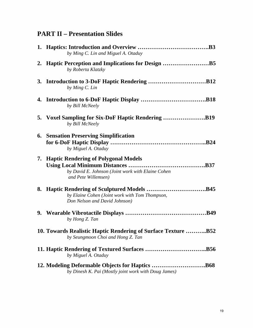
PART II – Presentation Slides 1. Haptics: Introduction and Overview ……………………………….B3
by Ming C. Lin and Miguel A. Otaduy
2. Haptic Perception and Implications for Design ……………………B5 by Roberta Klatzky
3. Introduction to 3-DoF Haptic Rendering …………………………B12 by Ming C. Lin
4. Introduction to 6-DoF Haptic Display …………………………….B18 by Bill McNeely
5. Voxel Sampling for Six-DoF Haptic Rendering ………………….B19 by Bill McNeely
6. Sensation Preserving Simplification for 6-DoF Haptic Display …………………………………………..B24
by Miguel A. Otaduy
7. Haptic Rendering of Polygonal Models Using Local Minimum Distances ………………………………….B37
by David E. Johnson (Joint work with Elaine Cohen and Pete Willemsen)
8. Haptic Rendering of Sculptured Models ………………………….B45 by Elaine Cohen (Joint work with Tom Thompson, Don Nelson and David Johnson)
9. Wearable Vibrotactile Displays ……………………………………B49 by Hong Z. Tan
10. Towards Realistic Haptic Rendering of Surface Texture ………..B52 by Seungmoon Choi and Hong Z. Tan
11. Haptic Rendering of Textured Surfaces …………………………..B56 by Miguel A. Otaduy
12. Modeling Deformable Objects for Haptics ……………………….B68 by Dinesh K. Pai (Mostly joint work with Doug James)
19

13. Reality-based Modeling for Haptics and Multimodal Displays …………………………………………..B73
by Dinesh K. Pai
14. Applications in Scientific Visualization …………………………...B80 by Russell M. Taylor II
15. Haptic Interaction with Fluid Media ……………………………...B87 by William Baxter and Ming C. Lin
20

PREFACE
To date, most human–computer interactive systems have focused primarily on the graphical rendering of visual information and, to a lesser extent, on the display of auditory information. Among all senses, the human haptic system provides unique and bidirectional communication between humans and their physical environment. Extending the frontier of visual computing, haptic interfaces, or force feedback devices, have the potential to increase the quality of human-computer interaction by accommodating the sense of touch. They provide an attractive augmentation to visual display and enhance the level of understanding of complex data sets. They have been effectively used for a number of applications including molecular docking, manipulation of nano-materials, surgical training, virtual prototyping and digital sculpting. Compared with visual and auditory display, haptic rendering has extremely demanding computational requirements. In order to maintain a stable system while displaying smooth and realistic forces and torques, haptic update rates of 1 KHz or more are typically used. Haptics presents many new challenges to researchers and developers in computer graphics and interactive techniques. Some of the critical issues include the development of novel data structures to encode shape and material properties, as well as new techniques for data processing, information analysis, physical modeling, and haptic visualization. This course will examine some of the latest developments on haptic rendering and applications, while looking forward to exciting future research in this area. We will present novel haptic rendering algorithms and innovative applications that take advantage of haptic interaction sensory modality. Specifically we will discuss different rendering techniques for various geometric representations (e.g. point-based, volumetric, polygonal, multiresolution, NURBS, distance fields, etc) and physical properties (rigid bodies, deformable models, fluid medium, etc), as well as textured surfaces and full-body interaction (e.g. wearable haptics). We will also show how psychophysics of touch can provide the foundational design guidelines for developing perceptually driven force models and discuss issues to consider in validating new rendering techniques and evaluating haptic interfaces. In addition, we will also look at different approaches to design touch-enabled interfaces for various applications, ranging from medical training, model design and maintainability analysis for virtual prototyping, scientific visualization, 3D painting and mesh editing, to data acquisition for multi-modal display. These recent advances indicate promising potentials that haptic interfaces together with interactive 3D graphics can offer a faster and more natural way of interacting with virtual environments and complex datasets in diverse applications.
Ming C. Lin and Miguel A. Otaduy
21

22

RECENT ADVANCES IN HAPTIC RENDERING AND APPLICATIONS Supplementary Course Notes PART I – Tutorial and Survey Chapters Ming C. Lin University of North Carolina at Chapel Hill Miguel A. Otaduy ETH Zurich
A1

A2

Introduction to Haptic Rendering
Miguel A. Otaduy Ming C. Lin
Department of Computer Science
University of North Carolina at Chapel Hill
1 Why Haptic Rendering?
For a long time, human beings have dreamed of a virtual world where it is possible to interact with syntheticentities as if they were real. To date, the advances in computer graphics allow us to see virtual objectsand avatars, to hear them, to move them, and to touch them. It has been shown that the ability to touchvirtual objects increases the sense of presence in virtual environments [Insko 2001].
Haptic rendering offers important applicability in engineering and medical training tasks. In this chapterwe introduce the concept of haptic rendering, and we briefly describe some of the basic techniques andapplications. In the first section we define some terminology, discuss the evolution of the research in hapticrendering, and introduce practical applications.
1.1 Definitions
The term haptic (from the Greek haptesthai, meaning “to touch”) is the adjective used to describe somethingrelating to or based on the sense of touch. Haptic is to touching as visual is to seeing and as auditory isto hearing [Fisher et al. 2004].
As described by Klatzky and Lederman [Klatzky and Lederman 2003], touch is one of the main avenues ofsensation, and it can be divided into cutaneous, kinesthetic, and haptic systems, based on the underlyingneural inputs. The cutaneous system employs receptors embedded in the skin, while the kinestheticsystem employs receptors located in muscles, tendons, and joints. The haptic sensory system employsboth cutaneous and kinesthetic receptors, but it differs in the sense that it is associated with an activeprocedure. Touch becomes active when the sensory inputs are combined with controlled body motion. Forexample, cutaneous touch becomes active when we explore a surface or grasp an object, while kinesthetictouch becomes active when we manipulate an object and touch other objects with it.
Haptic rendering is defined as the process of computing and generating forces in response to user interac-tions with virtual objects [Salisbury et al. 1995]. Several haptic rendering algorithms consider the paradigmof touching virtual objects with a single contact point. Rendering algorithms that follow this descriptionare called 3-DoF haptic rendering algorithms, because a point in 3D has only three DoFs. Other hapticrendering algorithms deal with the problem of rendering the forces and torques arising from the interactionof two virtual objects. This problem is called 6-DoF haptic rendering, because the grasped object has sixDoFs (position and orientation in 3D), and the haptic feedback comprises 3D force and torque. When weeat with a fork, write with a pen, or open a lock with a key, we are moving an object in 3D, and we feelthe interaction with other objects. This is, in essence, 6-DoF object manipulation with force-and-torquefeedback. Fig. 1 shows an example of a user experiencing haptic rendering. When we manipulate an objectand touch other objects with it, we perceive cutaneous feedback as the result of grasping, and kinestheticfeedback as the result of contact between objects.
A3

1 WHY HAPTIC RENDERING? 2
Figure 1: Example of Haptic Rendering. A person manipulates a virtual jaw using a haptic device(shown on the right of the image), and the interaction between jaws is displayed both visually and haptically.
1.2 From Telerobotics to Haptic Rendering
In 1965, Ivan Sutherland [Sutherland 1965] proposed a multimodal display that would incorporate hapticfeedback into the interaction with virtual worlds. Before that, haptic feedback had already been used mainlyin two applications: flight simulators and master-slave robotic teleoperation. The early teleoperator systemshad mechanical linkages between the master and the slave. But, in 1954, Goertz and Thompson [Goertzand Thompson 1954] developed an electrical servomechanism that received feedback signals from sensorsmounted on the slave and applied forces to the master, thus producing haptic feedback.
From there, haptic interfaces evolved in multiple directions, but there were two major breakthroughs.The first breakthrough was the idea of substituting the slave robot by a simulated system, in whichforces were computed using physically based simulations. The GROPE project at the University of NorthCarolina at Chapel Hill [Brooks, Jr. et al. 1990], lasting from 1967 to 1990, was the first one to addressthe synthesis of force feedback from simulated interactions. In particular, the aim of the project was toperform real-time simulation of 3D molecular-docking forces. The second breakthrough was the adventof computer-based Cartesian control for teleoperator systems [Bejczy and Salisbury 1980], enabling aseparation of the kinematic configurations of the master and the slave. Later, Cartesian control wasapplied to the manipulation of simulated slave robots [Kim and Bejczy 1991].
Those first haptic systems were able to simulate the interaction of simple virtual objects only. Perhaps thefirst project to target computation of forces in the interaction with objects with rich geometric informationwas Minsky’s Sandpaper [Minsky et al. 1990]. Minsky et al. developed a planar force feedback system thatallowed the exploration of textures. A few years after Minsky’s work, Zilles and Salisbury presented analgorithm for 3-DoF haptic rendering of polygonal models [Zilles and Salisbury 1995]. Almost in parallelwith Zilles and Salisbury’s work, Massie and Salisbury [Massie and Salisbury 1994] designed the PHANToM,a stylus-based haptic interface that was later commercialized and has become one of the most commonlyused force-feedback devices. But in the late ’90s, research in haptic rendering revived one of the problemsthat first inspired virtual force feedback: 6-DoF haptic rendering or, in other words, grasping of a virtualobject and synthesis of kinesthetic feedback of the interaction between this object and its environment.
A4

1 WHY HAPTIC RENDERING? 3
Research in the field of haptics in the last 35 years has covered many more areas than what we havesummarized here. [Burdea 1996] gives a general survey of the field of haptics and [McLaughlin et al. 2002]discuss current research topics.
1.3 Haptic Rendering for Virtual Manipulation
Certain professional activities, such as training for high-risk operations or pre-production prototype testing,can benefit greatly from simulated reproductions. The fidelity of the simulated reproductions depends,among other factors, on the similarity of the behaviors of real and virtual objects. In the real world,solid objects cannot interpenetrate. Contact forces can be interpreted mathematically as constraint forcesimposed by penetration constraints. However, unless penetration constraints are explicitly imposed, virtualobjects are free to penetrate each other in virtual environments. Indeed, one of the most disconcertingexperiences in virtual environments is to pass through virtual objects [Insko et al. 2001; Slater and Usoh1993]. Virtual environments require the simulation of non-penetrating rigid body dynamics, and thisproblem has been extensively explored in the robotics and computer graphics literature [Baraff 1992;Mirtich 1996].
It has been shown that being able to touch physical replicas of virtual objects (a technique known aspassive haptics [Insko 2001]) increases the sense of presence in virtual environments. This conclusion canprobably be generalized to the case of synthetic cutaneous feedback of the interaction with virtual objects.As reported by Brooks et al. [Brooks, Jr. et al. 1990], kinesthetic feedback radically improved situationawareness in virtual 3D molecular docking. Kinesthetic feedback has proved to enhance task performancein applications such as telerobotic object assembly [Hill and Salisbury 1977], virtual object assembly [Ungeret al. 2002], and virtual molecular docking [Ouh-Young 1990]. In particular, task completion time is shorterwith kinesthetic feedback in docking operations but not in prepositioning operations.
To summarize, haptic rendering is especially useful in particular examples of training for high-risk oper-ations or pre-production prototype testing activities that involve intensive object manipulation and inter-action with the environment. Such examples include minimally invasive or endoscopic surgery [Edmondet al. 1997; Hayward et al. 1998] and virtual prototyping for assembly and maintainability assessment [Mc-Neely et al. 1999; Chen 1999; Andriot 2002; Wan and McNeely 2003]. Force feedback becomes particularlyimportant and useful in situations with limited visual feedback.
1.4 3-DoF and 6-DoF Haptic Rendering
Much of the existing work in haptic rendering has focused on 3-DoF haptic rendering [Zilles and Salisbury1995; Ruspini et al. 1997; Thompson et al. 1997; Gregory et al. 1999; Ho et al. 1999]. Given a virtual objectA and the 3D position of a point p governed by an input device, 3-DoF haptic rendering can be summarizedas finding a contact point p′ constrained to the surface of A. The contact force will be computed as afunction of p and p′. In a dynamic setting, and assuming that A is a polyhedron with n triangles,the problem of finding p′ has an O(n) worst-case complexity. Using spatial partitioning strategies andexploiting motion coherence, however, the complexity becomes O(1) in many practical situations [Gregoryet al. 1999].
This reduced complexity has made 3-DoF haptic rendering an attractive solution for many applicationswith virtual haptic feedback, such as: sculpting and deformation [Dachille et al. 1999; Gregory et al. 2000a;McDonnell et al. 2001], painting [Johnson et al. 1999; Gregory et al. 2000a; Foskey et al. 2002], volumevisualization [Avila and Sobierajski 1996], nanomanipulation [Taylor et al. 1993], and training for diversesurgical operations [Kuhnapfel et al. 1997; Gibson et al. 1997]. In each of these applications, the interactionbetween the subject and the virtual objects is sufficiently captured by a point-surface contact model.
In 6-DoF manipulation and exploration, however, when a subject grasps an object and touches otherobjects in the environment, the interaction generally cannot be modeled by a point-surface contact. Onereason is the existence of multiple contacts that impose multiple simultaneous non-penetration constraints
A5

2 THE CHALLENGES 4
on the grasped object. In a simple 6-DoF manipulation example, such as the insertion of a peg in a hole,the grasped object (i.e., the peg) collides at multiple points with the rest of the scene (i.e., the walls ofthe hole and the surrounding surface). This contact configuration cannot be modeled as a point-objectcontact. Another reason is that the grasped object presents six DoFs, 3D translation and rotation, asopposed to the three DoFs of a point. The feasible trajectories of the peg are embedded in a 6-dimensionalspace with translational and rotational constraints, that cannot be captured with three DoFs.
Note that some cases of object-object interaction have been modeled in practice by ray-surface con-tact [Basdogan et al. 1997]. In particular, several surgical procedures are performed with 4-DoF tools (e.g.,laparoscopy), and this constraint has been exploited in training simulators with haptic feedback [Cavusogluet al. 2002]. Nevertheless, these approximations are valid only in a limited number of situations and cannotcapture full 6-DoF object manipulation.
2 The Challenges
Haptic rendering is in essence an interactive activity, and its realization is mostly handicapped by twoconflicting challenges: high required update rates and the computational cost. In this section we outlinethe computational pipeline of haptic rendering, and we discuss associated challenges.
2.1 Haptic Rendering Pipeline
Haptic rendering comprises two main tasks. One of them is the computation of the position and/ororientation of the virtual probe grasped by the user. The other one is the computation of contact forceand/or torque that are fed back to the user. The existing methods for haptic rendering can be classifiedinto two large groups based on their overall pipelines.
In direct rendering methods [Nelson et al. 1999; Gregory et al. 2000b; Kim et al. 2003; Johnson andWillemsen 2003; Johnson and Willemsen 2004], the position and/or orientation of the haptic device areapplied directly to the grasped probe. Collision detection is performed between the grasped probe and thevirtual objects, and collision response is applied to the grasped probe as a function of object separation orpenetration depth. The resulting contact force and/or torque are directly fed back to the user.
In virtual coupling methods [Chang and Colgate 1997; Berkelman 1999; McNeely et al. 1999; Ruspiniand Khatib 2000; Wan and McNeely 2003], the position and/or orientation of the haptic device are setas goals for the grasped probe, and a virtual viscoelastic coupling [Colgate et al. 1995] produces a forcethat attracts the grasped probe to its goals. Collision detection and response are performed between thegrasped probe and the virtual objects. The coupling force and/or torque are combined with the collisionresponse in order to compute the position and/or orientation of the grasped probe. The same couplingforce and/or torque are fed back to the user.
In Sec. 8, I describe the different existing methods for 6-DoF haptic rendering in more detail, and Idiscuss their advantages and disadvantages. Also, as explained in more detail in Sec. 4, there are twomajor types of haptic devices, and for each type of device the rendering pipeline presents slight variations.Impedance-type devices read the position and orientation of the handle of the device and control the forceand torque applied to the user. Admittance-type devices read the force and torque applied by the userand control the position and orientation of the handle of the device.
2.2 Force Update Rate
The ultimate goal of haptic rendering is to provide force feedback to the user. This goal is achieved bycontrolling the handle of the haptic device, which is in fact the end-effector of a robotic manipulator. Whenthe user holds the handle, he or she experiences kinesthetic feedback. The entire haptic rendering system
A6

2 THE CHALLENGES 5
is regarded as a mechanical impedance that sets a transformation between the position and velocity of thehandle of the device and the applied force.
The quality of haptic rendering can be measured in terms of the dynamic range of impedances that canbe simulated in a stable manner [Colgate and Brown 1994]. When the user moves the haptic device in freespace, the perceived impedance should be very low (i.e., small force), and when the grasped virtual objecttouches other rigid objects, the perceived impedance should be high (i.e., high stiffness and/or dampingof the constraint). The quality of haptic rendering can also be measured in terms of the responsiveness ofthe simulation [Brooks, Jr. et al. 1990; Berkelman 1999]. In free-space motion the grasped probe shouldrespond quickly to the motion of the user. Similarly, when the grasped probe collides with a virtual wall,the user should stop quickly, in response to the motion constraint.
With impedance-type devices, virtual walls are implemented as large stiffness values in the simulation.In haptic rendering, the user is part of a closed-loop sampled dynamic system [Colgate and Schenkel 1994],along with the device and the virtual environment, and the existence of sampling and latency phenomenacan induce unstable behavior under large stiffness values. System instability is directly perceived by theuser in the form of disturbing oscillations. A key factor for achieving a high dynamic range of impedances(i.e., stiff virtual walls) while ensuring stable rendering is the computation of feedback forces at a highupdate rate [Colgate and Schenkel 1994; Colgate and Brown 1994]. Brooks et al. [Brooks, Jr. et al. 1990]reported that, in the rendering of textured surfaces, users were able to perceive performance differences atforce update rates between 500Hz and 1kHz.
A more detailed description of the stability issues involved in the synthesis of force feedback, and adescription of related work, are given in Sec. 4. Although here we have focused on impedance-type hapticdevices, similar conclusions can be drawn for admittance-type devices (See [Adams and Hannaford 1998]and Sec. 4).
2.3 Contact Determination
The computation of non-penetrating rigid-body dynamics of the grasped probe and, ultimately, synthesis ofhaptic feedback require a model of collision response. Forces between the virtual objects must be computedfrom contact information. Determining whether two virtual objects collide (i.e., intersect) is not enough,and additional information, such as penetration distance, contact points, contact normals, and so forth,need to be computed. Contact determination describes the operation of obtaining the contact informationnecessary for collision response [Baraff 1992].
For two interacting virtual objects, collision response can be computed as a function of object separation,with worst-case cost O(mn), or penetration depth, with a complexity bound of Ω(m3n3). But collisionresponse can also be applied at multiple contacts simultaneously. Given two objects A and B with m andn triangles respectively, contacts can be defined as pairs of intersecting triangles or pairs of triangles insidea distance tolerance. The number of pairs of intersecting triangles is O(mn) in worst-case pathologicalcases, and the number of pairs of triangles inside a tolerance can be O(mn) in practical cases. In Sec. 5,we discuss in more detail existing techniques for determining the contact information.
The cost of contact determination depends largely on factors such as the convexity of the interactingobjects or the contact configuration. There is no direct connection between the polygonal complexityof the objects and the cost of contact determination but, as a reference, existing exact collision detectionmethods can barely execute contact queries for force feedback between pairs of objects with 1, 000 trianglesin complex contact scenarios [Kim et al. 2003] at force update rates of 1kHz.
Contact determination becomes particularly expensive in the interaction between textured surfaces.Studies have been done on the highest texture resolution that can be perceived through cutaneous touch,but there are no clear results regarding the highest resolution that can be perceived kinesthetically throughan intermediate object. It is known that, in the latter case, texture-induced roughness perception is encodedin vibratory motion [Klatzky and Lederman 2002]. Psychophysics researchers report that 1mm textures
A7

3 PSYCHOPHYSICS OF HAPTICS 6
are clearly perceivable, and perceived roughness appears to be even greater with finer textures [Ledermanet al. 2000]. Based on Shannon’s sampling theorem, a 10cm × 10cm plate with a sinusoidal texture of1mm in orthogonal directions is barely correctly sampled with 40, 000 vertices. This measure gives an ideaof the triangulation density required for capturing texture information of complex textured objects. Notethat the triangulation density may grow by orders of magnitude if the textures are not sinusoidal and/orif information about normals and curvatures is also needed.
3 Psychophysics of Haptics
In the design of contact determination algorithms for haptic rendering, it is crucial to understand thepsychophysics of touch and to account for perceptual factors. The structure and behavior of humantouch have been studied extensively in the field of psychology. The topics analyzed by researchers includecharacterization of sensory phenomena as well as cognitive and memory processes.
Haptic perception of physical properties includes a first step of stimulus registration and communicationto the thalamus, followed by a second step of higher-level processing. Perceptual measures can be origi-nated by individual mechanoreceptors but also by the integration of inputs from populations of differentsensory units [Klatzky and Lederman 2003]. Klatzky and Lederman [Klatzky and Lederman 2003] discussobject and surface properties that are perceived through the sense of touch (e.g., texture, hardness, andweight) and divide them between geometric and material properties. They also analyze active exploratoryprocedures (e.g., lateral motion, pressure, or unsupported holding) typically conducted by subjects in orderto capture information about the different properties.
Knowing the exploratory procedure(s) associated with a particular object or surface property, researchershave studied the influence of various parameters on the accuracy and magnitude of sensory outputs.Perceptual studies on tactile feature detection and identification, as well as studies on texture or roughnessperception are of particular interest for haptic rendering. In this section we summarize existing researchon perception of surface features and perception of roughness, and then we discuss issues associated withthe interaction of visual and haptic modalities.
3.1 Perception of Surface Features
Klatzky and Lederman describe two different exploratory procedures followed by subjects in order tocapture shape attributes and identify features and objects. In haptic glance [Klatzky and Lederman 1995],subjects extract information from a brief haptic exposure of the object surface. Then they perform higher-level processing for determining the identity of the object or other attributes. In contour following [Klatzkyand Lederman 2003], subjects create a spatiotemporal map of surface attributes, such as curvature, thatserves as the pattern for feature identification. Contact determination algorithms attempt to describethe geometric interaction between virtual objects. The instantaneous nature of haptic glance [Klatzkyand Lederman 1995] makes it strongly dependent on purely geometric attributes, unlike the temporaldependency of contour following.
Klatzky and Lederman [Klatzky and Lederman 1995] conducted experiments in which subjects wereinstructed to identify objects from brief cutaneous exposures (i.e., haptic glances). Subjects had an advancehypothesis of the nature of the object. The purpose of the study was to discover how, and how well, subjectsidentify objects from brief contact. According to Klatzky and Lederman, during haptic glance a subjecthas access to three pieces of information: roughness, compliance, and local features. Roughness andcompliance are material properties that can be extracted from lower-level processing, while local featurescan lead to object identification by feature matching during higher-level processing. In the experiments,highest identification accuracy was achieved with small objects, whose shapes fit on a fingertip. Klatzky andLederman concluded that large contact area helped in the identification of textures or patterns, although itwas better to have a stimulus of a size comparable to or just slightly smaller than that of the contact area
A8

3 PSYCHOPHYSICS OF HAPTICS 7
for the identification of geometric surface features. The experiments conducted by Klatzky and Ledermanposit an interesting relation between feature size and contact area during cutaneous perception.
Okamura and Cutkosky [Okamura and Cutkosky 1999; Okamura and Cutkosky 2001] analyzed featuredetection in robotic exploration, which can be regarded as a case of object-object interaction. Theycharacterized geometric surface features based on the ratios of their curvatures to the radii of the roboticfingertips acquiring the surface data. They observed that a larger fingertip, which provides a larger contactarea, can miss small geometric features. To summarize, the studies by Klatzky and Lederman [Klatzkyand Lederman 1995] and Okamura and Cutkosky [Okamura and Cutkosky 1999; Okamura and Cutkosky2001] lead to the observation that human haptic perception of the existence of a geometric surface featuredepends on the ratio between the contact area and the size of the feature, not the absolute size of thefeature itself. This observation has driven the design of multiresolution contact determination algorithmsfor haptic rendering [Otaduy and Lin 2003b].
3.2 Perception of Texture and Roughness
Klatzky and Lederman [Klatzky and Lederman 2003] describe a textured surface as a surface with pro-tuberant elements arising from a relatively homogeneous substrate. Interaction with a textured surfaceresults in perception of roughness. Existing research on the psychophysics of texture perception indicates aclear dichotomy of exploratory procedures: (a) perception of texture with the bare skin, and (b) perceptionthrough an intermediate (rigid) object, a probe.
Most of the research efforts have been directed towards the characterization of cutaneous perceptionof textures. Katz [Katz 1989] suggested that roughness is perceived through a combination of spatialand vibratory codes during direct interaction with the skin. More recent evidence demonstrates thatstatic pressure distribution plays a dominant role in perception of coarse textures (features larger than1mm) [Lederman 1974; Connor and Johnson 1992], but motion-induced vibration is necessary for perceivingfine textures [LaMotte and Srinivasan 1991; Hollins and Risner 2000].
As pointed out by Klatzky and Lederman [Klatzky and Lederman 2002], in object-object interactionroughness is encoded in vibratory motion transmitted to the subject. In the last few years, Klatzky andLederman have directed experiments that analyze the influence of several factors on roughness perceptionthrough a rigid probe. Klatzky et al. [Klatzky et al. 2003] distinguished three types of factors that may affectthe perceived magnitude of roughness: interobject physical interaction, skin- and limb-induced filteringprior to cutaneous and kinesthetic perception, and higher-level factors such as efferent commands. Thedesign of contact determination and collision response algorithms for haptic texture rendering is mostlyconcerned with factors related to the physical interaction between objects: object geometry [Ledermanet al. 2000; Klatzky et al. 2003], applied force [Lederman et al. 2000], and exploratory speed [Ledermanet al. 1999; Klatzky et al. 2003]. The influence of these factors has been addressed in the design of haptictexture rendering algorithms [Otaduy et al. 2004].
The experiments conducted by Klatzky and Lederman to characterize roughness perception [Klatzky andLederman 2002] used a common setup: subjects explored a textured plate with a probe with a sphericaltip, and then they reported a subjective measure of roughness. Plates of jittered raised dots were used,and the mean frequency of dot distribution was one of the variables in the experiments. The resulting datawas analyzed by plotting subjective roughness values vs. dot interspacing in logarithmic graphs.
Klatzky and Lederman [Klatzky and Lederman 1999] compared graphs of roughness vs. texture spacing(a) with finger exploration and (b) with a rigid probe. They concluded that, in the range of their data,roughness functions were best fit by linear approximations in finger exploration and by quadratic approx-imations in probe-based exploration. In other words, when perceived through a rigid spherical probe,roughness initially increases as texture spacing increases, but, after reaching a maximum roughness value,it decreases again. Based on this finding, the influence of other factors on roughness perception can becharacterized by the maximum value of roughness and the value of texture spacing at which this maximum
A9

4 STABILITY AND CONTROL THEORY APPLIED TO HAPTIC RENDERING 8
takes place.
Lederman et al. [Lederman et al. 2000] demonstrated that the diameter of the spherical probe playsa crucial role in the maximum value of perceived roughness and the location of the maximum. Theroughness peak is higher for smaller probes, and it occurs at smaller texture spacing values. Ledermanet al. [Lederman et al. 2000] also studied the influence of the applied normal force during exploration.Roughness is higher for larger force, but the influence on the location of the peak is negligible. The effectof exploratory speed was studied by Lederman et al. [Lederman et al. 1999]. They found that the peak ofroughness occurs at larger texture spacing for higher speed. Also, with higher speed, textured plates feelsmoother at small texture spacing, and rougher at large spacing values. The studies reflected that speedhas a stronger effect in passive interaction than in active interaction.
3.3 Haptic and Visual Cross-modal Interaction
Haptic rendering is often presented along with visual display. Therefore, it is important to understand theissues involved in cross-modal interaction. Klatzky and Lederman [Klatzky and Lederman 2003] discussaspects of visual and haptic cross-modal integration from two perspectives: attention and dominance.
Spence et al. [Spence et al. 2000] have studied how visual and tactile cues can influence a subject’sattention. Their conclusions are that visual and tactile cues are treated together in a single attentionalmechanism, and wrong attention cues can affect perception negatively.
Sensory dominance is usually studied by analyzing perceptual discrepancies in situations where cross-modal integration yields a unitary perceptual response. One example of relevance for this dissertationis the detection of object collision. During object manipulation, humans determine whether two objectsare in contact based on a combination of visual and haptic cues. Early studies of sensory dominanceseemed to point to a strong dominance of visual cues over haptic cues [Rock and Victor 1964], but in thelast decades psychologists agree that sensory inputs are weighted based on their statistical reliability orrelative appropriateness, measured in terms of accuracy, precision, and cue availability [Heller et al. 1999;Ernst and Banks 2001; Klatzky and Lederman 2003].
The design of contact determination algorithms can also benefit from existing studies on the visualperception of collisions in computer animations. O’Sullivan and her colleagues [O’Sullivan et al. 1999;O’Sullivan and Dingliana 2001; O’Sullivan et al. 2003] have investigated different factors affecting visualcollision perception, including eccentricity, separation, distractors, causality, and accuracy of simulationresults. Basing their work on a model of human visual perception validated by psychophysical experiments,they demonstrated the feasibility of using these factors for scheduling interruptible collision detection amonglarge numbers of visually homogeneous objects.
4 Stability and Control Theory Applied to Haptic Rendering
In haptic rendering, the human user is part of the dynamic system, along with the haptic device andthe computer implementation of the virtual environment. The complete human-in-the-loop system canbe regarded as a sampled-data system [Colgate and Schenkel 1994], with a continuous component (theuser and the device) and a discrete one (the implementation of the virtual environment and the devicecontroller). Stability becomes a crucial feature, because instabilities in the system can produce oscillationsthat distort the perception of the virtual environment, or uncontrolled motion of the device that can evenhurt the user. In Sec. 2.2, we have briefly discussed the importance of stability for haptic rendering, andwe have introduced the effect of the force update rate on stability. In this section we review and discussin more detail existing work in control theory related to stability analysis of haptic rendering.
A10

4 STABILITY AND CONTROL THEORY APPLIED TO HAPTIC RENDERING 9
4.1 Mechanical Impedance Control
The concept of mechanical impedance extends the notion of electrical impedance and refers to the quotientbetween force and velocity. Hogan [Hogan 1985] introduced the idea of impedance control for contact tasksin manipulation. Earlier techniques controlled contact force, robot velocity, or both, but Hogan suggestedcontrolling directly the mechanical impedance, which governs the dynamic properties of the system. Whenthe end effector of a robot touches a rigid surface, it suffers a drastic change of mechanical impedance,from low impedance in free space, to high impedance during contact. This phenomenon imposes seriousdifficulties on earlier control techniques, inducing instabilities.
The function of a haptic device is to display the feedback force of a virtual world to a human user. Hapticdevices present control challenges very similar to those of manipulators for contact tasks. As introducedin Sec. 2.1, there are two major ways of controlling a haptic device: impedance control and admittancecontrol. In impedance control, the user moves the device, and the controller produces a force dependenton the interaction in the virtual world. In admittance control, the user applies a force to the device, andthe controller moves the device according to the virtual interaction.
In both impedance and admittance control, high control gains can induce instabilities. In impedancecontrol, instabilities may arise in the simulation of stiff virtual surfaces. The device must react withlarge changes in force to small changes in the position. Conversely, in admittance control, rendering astiff virtual surface is not a challenging problem, because it is implemented as a low controller gain. Inadmittance control, however, instabilities may arise during free-space motion in the virtual world, becausethe device must move at high velocities under small applied forces, or when the device rests on a stiffphysical surface. Impedance and admittance control can therefore be regarded as complementary controltechniques, best suited for opposite applications. Following the unifying framework presented by Adamsand Hannaford [Adams and Hannaford 1998], Contact determination and force computation algorithmsare often independent of the control strategy.
4.2 Stable Rendering of Virtual Walls
Since the introduction of impedance control by Hogan [Hogan 1985], the analysis of the stability of hapticdevices and haptic rendering algorithms has focused on the problem of rendering stiff virtual walls. Thiswas known to be a complex problem at early stages of research in haptic rendering [Kilpatrick 1976], butimpedance control simplified the analysis, because a virtual wall can be modeled easily using stiffness andviscosity parameters.
Ouh-Young [Ouh-Young 1990] created a discrete model of the Argonne ARM and the human arm andanalyzed the influence of force update rate on the stability and responsiveness of the system. Minsky,Brooks, et al. [Minsky et al. 1990; Brooks, Jr. et al. 1990] observed that update rates as high as 500Hz or1kHz might be necessary in order to achieve stability.
Colgate and Brown [Colgate and Brown 1994] coined the term Z-Width for describing the range ofmechanical impedances that a haptic device can render while guaranteeing stability. They concluded thatphysical dissipation is essential for achieving stability and that the maximum achievable virtual stiffnessis proportional to the update rate. They also analyzed the influence of position sensors and quantization,and concluded that sensor resolution must be maximized and the velocity signal must be filtered.
Almost in parallel, Salcudean and Vlaar [Salcudean and Vlaar 1994] studied haptic rendering of virtualwalls, and techniques for improving the fidelity of the rendering. They compared a continuous model of avirtual wall with a discrete model that accounts for differentiation of the position signal. The continuousmodel is unconditionally stable, but this is not true for the discrete model. Moreover, in the discrete modelfast damping of contact oscillations is possible only with rather low contact stiffness and, as indicated byColgate and Brown too [Colgate and Brown 1994], this value of stiffness is proportional to the updaterate. Salcudean and Vlaar proposed the addition of braking pulses, proportional to collision velocity, forimproving the perception of virtual walls.
A11

4 STABILITY AND CONTROL THEORY APPLIED TO HAPTIC RENDERING 10
4.3 Passivity and Virtual Coupling
A subsystem is passive if it does not add energy to the global system. Passivity is a powerful tool foranalyzing stability of coupled systems, because the coupled system obtained from two passive subsystemsis always stable. Colgate and his colleagues were the first to apply passivity criteria to the analysis ofstability in haptic rendering of virtual walls [Colgate et al. 1993]. Passivity-based analysis has enabledseparate study of the behavior of the human subsystem, the haptic device, and the virtual environment inforce-feedback systems.
4.3.1 Human Sensing and Control Bandwidths
Hogan discovered that the human neuromuscular system exhibits externally simple, springlike behav-ior [Hogan 1986]. This finding implies that the human arm holding a haptic device can be regarded as apassive subsystem, and the stability analysis can focus on the haptic device and the virtual environment.
Note that human limbs are not passive in all conditions, but the bandwidth at which a subject canperform active motions is very low compared to the frequencies at which stability problems may arise.Some authors [Shimoga 1992; Burdea 1996] report that the bandwidth at which humans can performcontrolled actions with the hand or fingers is between 5 and 10Hz. On the other hand, sensing bandwidthcan be as high as 20 to 30Hz for proprioception, 400Hz for tactile sensing, and 5 to 10kHz for roughnessperception.
4.3.2 Passivity of Virtual Walls
Colgate and Schenkel [Colgate and Schenkel 1994] observed that the oscillations perceived by a haptic userduring system instability are a result of active behavior of the force-feedback system. This active behavioris a consequence of time delay and loss of information inherent in sampled-data systems, as suggested byothers before [Brooks, Jr. et al. 1990]. Colgate and Schenkel formulated passivity conditions in hapticrendering of a virtual wall. For that analysis, they modeled the virtual wall as a viscoelastic unilateralconstraint, and they accounted for the continuous dynamics of the haptic device, sampling of the positionsignal, discrete differentiation for obtaining velocity, and a zero-order hold of the output force. Theyreached a sufficient condition for passivity that relates the stiffness K and damping B of the virtual wall,the inherent damping b of the device, and the sampling period T :
b >KT
2+ B. (1)
4.3.3 Stability of Non-linear Virtual Environments
After deriving stability conditions for rendering virtual walls modeled as unilateral linear constraints,Colgate and his colleagues considered more complex environments [Colgate et al. 1995]. A general virtualenvironment is non-linear, and it presents multiple and variable constraints. Their approach enforces adiscrete-time passive implementation of the virtual environment and sets a multidimensional viscoelasticvirtual coupling between the virtual environment and the haptic display. In this way, the stability of thesystem is guaranteed as long as the virtual coupling is itself passive, and this condition can be analyzed usingthe same techniques as those used for virtual walls [Colgate and Schenkel 1994]. As a result of Colgate’svirtual coupling [Colgate et al. 1995], the complexity of the problem was shifted towards designing a passivesolution of virtual world dynamics. As noted by Colgate et al. [Colgate et al. 1995], one possible way toenforce passivity in rigid body dynamics simulation is to use implicit integration with penalty methods.
Adams and Hannaford [Adams and Hannaford 1998] provided a framework for analyzing stability withadmittance-type and impedance-type haptic devices. They derived stability conditions for coupled systemsbased on network theory. They also extended the concept of virtual coupling to admittance-type devices.
A12

5 COLLISION DETECTION 11
Miller et al. [Miller et al. 1990] extended Colgate’s passivity analysis techniques, relaxing the requirementof passive virtual environments but enforcing cyclo-passivity of the complete system. Hannaford and hiscolleagues [Hannaford et al. 2002] investigated the use of adaptive controllers instead of the traditionalfixed-value virtual couplings. They designed passivity observers and passivity controllers for dissipatingthe excess of energy generated by the virtual environment.
4.4 Multirate Approximation Techniques
Multirate approximation techniques, though simple, have been successful in improving the stability andresponsiveness of haptic rendering systems. The idea is to perform a full update of the virtual environmentat a low frequency (limited by computational resources and the complexity of the system) and to use asimplified approximation for performing high-frequency updates of force feedback.
Adachi [Adachi et al. 1995] proposed an intermediate representation for haptic display of complex polyg-onal objects. In a slow collision detection thread, he computed a plane that served as a unilateral constraintin the force-feedback thread. This technique was later adapted by Mark et al. [Mark et al. 1996], whointerpolated the intermediate representation between updates. This approach enables higher stiffness val-ues than approaches that compute the feedback force values at the rate imposed by collision detection.More recently, a similar multirate approach has been followed by many authors for haptic interaction withdeformable models [Astley and Hayward 1998; Cavusoglu and Tendick 2000; Duriez et al. 2004]. Ellis etal. [Ellis et al. 1997] produce higher-quality rendering by upsampling directly the output force values.
5 Collision Detection
Collision detection has received much attention in robotics, computational geometry, and computer graph-ics. Some researchers have investigated the problem of interference detection as a mechanism for indicatingwhether object configurations are valid or not. Others have tackled the problems of computing separationor penetration distances, with the objective of applying collision response in simulated environments. Theexisting work on collision detection can be classified based on the types of models handled: 2-manifoldpolyhedral models, polygon soups, curved surfaces, etc. In this section we focus on collision detection forpolyhedral models. The vast majority of the algorithms used in practice proceed in two steps: first theycull large portions of the objects that are not in close proximity, using spatial partitioning, hierarchicaltechniques, or visibility-based properties, and then they perform primitive-level tests.
In this section, we first describe the problems of interference detection and computation of separationdistance between polyhedra, with an emphasis on algorithms specialized for convex polyhedra. Thenwe survey algorithms for the computation of penetration depth, the use of hierarchical techniques, andmultiresolution collision detection. we conclude the section by covering briefly the use of graphics processorsfor collision detection and the topic of continuous collision detection. For more information on collisiondetection, please refer to surveys on the topic [Lin and Gottschalk 1998; Klosowski et al. 1998; Lin andManocha 2004].
5.1 Proximity Queries Between Convex Polyhedra
The property of convexity has been exploited in algorithms with sublinear cost for detecting interferenceor computing the closest distance between two polyhedra. Detecting whether two convex polyhedra inter-sect can be posed as a linear programming problem, searching for the coefficients of a separating plane.Well-known linear programming algorithms [Seidel 1990] can run in expected linear time due to the lowdimensionality of the problem.
The separation distance between two polyhedra A and B is equal to the distance from the origin tothe Minkowski sum of A and −B [Cameron and Culley 1986]. This property was exploited by Gilbert
A13

5 COLLISION DETECTION 12
et al. [Gilbert et al. 1988] in order to design a convex optimization algorithm (known as GJK) forcomputing the separation distance between convex polyhedra, with linear-time performance in practice.Cameron [Cameron 1997] modified the GJK algorithm to exploit motion coherence in the initialization ofthe convex optimization at every frame for dynamic problems, achieving nearly constant running-time inpractice.
Lin and Canny [Lin and Canny 1991; Lin 1993] designed an algorithm for computing separation distanceby tracking the closest features between convex polyhedra. Their algorithm “walks” on the surfaces of thepolyhedra until it finds two features that lie on each other’s Voronoi region. Exploiting motion coherenceand geometric locality, Voronoi marching runs in nearly constant time per frame. Mirtich [Mirtich 1998b]later improved the robustness of this algorithm.
Given polyhedra A and B with m and n polygons respectively, Dobkin and Kirkpatrick [Dobkin andKirkpatrick 1990] proposed an algorithm for interference detection with O(log m log n) time complexitythat uses hierarchical representations of the polyhedra. Others have also exploited the use of hierarchicalconvex representations along with temporal coherence in order to accelerate queries in dynamic scenes.Guibas et al. [Guibas et al. 1999] employ the inner hierarchies suggested by Dobkin and Kirkpatrick,but they perform faster multilevel walking. Ehmann and Lin [Ehmann and Lin 2000] employ a modifiedversion of Dobkin and Kirkpatrick’s outer hierarchies, computed using simplification techniques, along witha multilevel implementation of Lin and Canny’s Voronoi marching [Lin and Canny 1991].
5.2 Penetration Depth
The penetration depth between two intersecting polyhedra A and B is defined as the minimum transla-tional distance required for separating them. For intersecting polyhedra, the origin is contained in theMinkowski sum of A and −B, and the penetration depth is equal to the minimum distance from the originto the surface of the Minkowski sum. The computation of penetration depth can be Ω(m3n3) for generalpolyhedra [Dobkin et al. 1993].
Many researchers have restricted the computation of penetration depth to convex polyhedra. In com-putational geometry, Dobkin et al. [Dobkin et al. 1993] presented an algorithm for computing directionalpenetration depth, while Agarwal et al. [Agarwal et al. 2000] introduced a randomized algorithm for com-puting the penetration depth between convex polyhedra. Cameron [Cameron 1997] extended the GJKalgorithm [Gilbert et al. 1988] to compute bounds of the penetration depth, and van den Bergen [van denBergen 2001] furthered his work. Kim et al. [Kim et al. 2002a] presented an algorithm that computes alocally optimal solution of the penetration depth by walking on the surface of the Minkowski sum.
The fastest algorithms for computation of penetration depth between arbitrary polyhedra take advantageof discretization. Fisher and Lin [Fisher and Lin 2001] estimate penetration depth using distance fieldscomputed with fast marching level-sets. Hoff et al. [Hoff et al. 2001] presented an image-based algorithmimplemented on graphics hardware. On the other hand, Kim et al. [Kim et al. 2002b] presented analgorithm that decomposes the polyhedra into convex patches, computes the Minkowski sums of pairwisepatches, and then uses an image-based technique in order to find the minimum distance from the origin tothe surface of the Minkowski sums.
5.3 Hierarchical Collision Detection
The algorithms for collision detection between convex polyhedra are not directly applicable to non-convexpolyhedra or models described as polygon soups. Brute force checking of all triangle pairs, however,is usually unnecessary. Collision detection between general models achieves large speed-ups by usinghierarchical culling or spatial partitioning techniques that restrict the primitive-level tests. Over the lastdecade, bounding volume hierarchies (BVH) have proved successful in the acceleration of collision detectionfor dynamic scenes of rigid bodies. For an extensive description and analysis of the use of BVHs for collisiondetection, please refer to Gottschalk’s PhD dissertation [Gottschalk 2000].
A14

5 COLLISION DETECTION 13
Assuming that an object is described by a set of triangles T , a BVH is a tree of BVs, where each BVCi bounds a cluster of triangles Ti ∈ T . The clusters bounded by the children of Ci constitute a partitionof Ti. The effectiveness of a BVH is conditioned by ensuring that the branching factor of the tree is O(1)and that the size of the leaf clusters is also O(1). Often, the leaf BVs bound only one triangle. A BVHmay be created in a top-down manner, by successive partitioning of clusters, or in a bottom-up manner,by using merging operations.
In order to perform interference detection using BVHs, two objects are queried by recursively traversingtheir BVHs in tandem. Each recursive step tests whether a pair of BVs a and b, one from each hierarchy,overlap. If a and b do not overlap, the recursion branch is terminated. Otherwise, if they overlap, thealgorithm is applied recursively to their children. If a and b are both leaf nodes, the triangles within themare tested directly. This process can be generalized to other types of proximity queries as well.
One determining factor in the design of a BVH is the selection of the type of BV. Often there is atrade-off among the tightness of the BV (and therefore the culling efficiency), the cost of the collisiontest between two BVs, and the dynamic update of the BV (relevant for deformable models). Some ofthe common BVs, sorted approximately according to increasing query time, are: spheres [Quinlan 1994;Hubbard 1994], axis-aligned bounding boxes (AABB) [Beckmann et al. 1990], oriented bounding boxes(OBB) [Gottschalk et al. 1996], k-discrete-orientation polytopes (k-DOP) [Klosowski et al. 1998], convexhulls [Ehmann and Lin 2001], and swept sphere volumes (SSV) [Larsen et al. 2000]. BVHs of rigid bodiescan be computed as a preprocessing step, but deformable models require a bottom-up update of the BVsafter each deformation. Recently, James and Pai [James and Pai 2004] have presented the BD-tree, avariant of the sphere-tree data structure [Quinlan 1994] that can be updated in a fast top-down manner ifthe deformations are described by a small number of parameters.
5.4 Multiresolution Collision Detection
Multiresolution analysis of a function decomposes the function into a basic low-resolution representationand a set of detail terms at increasing resolutions. Wavelets provide a mathematical framework for definingmultiresolution analysis [Stollnitz et al. 1996].
Multiresolution representations of triangles meshes have drawn important attention in computer graph-ics. They have been defined in two major ways: following the mathematical framework of wavelets andsubdivision surfaces [Lounsbery et al. 1997; Eck et al. 1995] or following level-of-detail (LOD) simplificationtechniques (please refer to [Luebke et al. 2002] for a survey on the topic). LOD techniques present theadvantage of being applicable to arbitrary meshes, but they lack a well-defined metric of resolution. Theyconstruct the multiresolution representations starting from full-resolution meshes and applying sequencesof local simplification operations. LOD techniques can be divided into those that produce a discrete setof representations (static LODs), and those that produce continuously adaptive representations (dynamicLODs). Multiresolution or LOD techniques have been used in applications such as view-dependent render-ing [Hoppe 1997; Luebke and Erikson 1997], interactive editing of meshes [Zorin et al. 1997], or real-timedeformations [Debunne et al. 2001]. The idea behind multiresolution techniques is to select the resolu-tion or LOD of the representation in an adaptive manner based on perceptual parameters, availability ofcomputational resources, and so forth.
Multiresolution collision detection refers to the execution of approximate collision detection queriesusing adaptive object representations. Hubbard [Hubbard 1994] introduced the idea of using sphere-trees [Quinlan 1994] for multiresolution collision detection, refining the BVHs in a breadth-first manneruntil the time allocated for collision detection expires. In a sphere-tree each level of the BVH can beregarded as an implicit approximation of the given mesh, by defining the surface as a union of spheres.Unlike LOD techniques, in which simplification operations minimize surface deviation, sphere-trees addextraneous “bumpiness” to the surface, and this characteristic can hurt collision response.
O’Sullivan and Dingliana [O’Sullivan and Dingliana 2001] have incorporated perceptual parameters into
A15

6 RIGID BODY SIMULATION 14
the refinement of sphere-trees. They insert pairs of spheres that test positive for collision in a priorityqueue sorted according to perceptual metrics (e.g., local relative velocity, distance to the viewer, etc.). Inthis way the adaptive refinement focuses on areas of the objects where errors are most noticeable.
The use of multiresolution representations for haptic rendering has also been investigated by severalresearchers. Pai and Reissel [Pai and Reissel 1997] investigated the use of multiresolution image curvesfor 2D haptic interaction. El-Sana and Varshney [El-Sana and Varshney 2000] applied LOD techniques to3-DoF haptic rendering. They created a multiresolution representation of the haptically rendered object asa preprocessing step and, at runtime, they represented the object at high resolution near the probe pointand at low resolution further away. Their approach does not extend naturally to the interaction betweentwo objects, since multiple disjoint contacts can occur simultaneously at widely varying locations withoutmuch spatial coherence. Otaduy and Lin [Otaduy and Lin 2003b; Otaduy and Lin 2003a] introducedcontact levels of detail, dual hierarchical representations for multiresolution collision detection, and theyapplied them to 6-DoF haptic rendering, producing a sensation-preserving simplified rendering.
5.5 Other Techniques for Collision Detection
We briefly cover two additional topics with potential applicability in haptic rendering: the use of graphicsprocessors for collision detection, and continuous collision detection.
5.5.1 Use of Graphics Processors for Collision Detection
The processing capability of GPUs is growing at a rate higher than Moore’s law [Govindaraju et al.2003], and this circumstance has generated an increasing use of GPUs for general-purpose computation,including collision detection. Rasterization hardware enables high performance of image-based collisiondetection algorithms. Hoff et al. [Hoff et al. 2001] presented an algorithm for estimating penetration depthbetween deformable polygons using distance fields computed on graphics hardware. Others have formulatedcollision detection queries as visibility problems. Lombardo et al. [Lombardo et al. 1999] intersected acomplex object against a simpler one using the view frustum and clipping planes, and they detectedintersecting triangles by exploiting OpenGL capabilities. More recently, Govindaraju et al. [Govindarajuet al. 2003] have designed an algorithm that performs series of visibility queries and achieves fast cullingof non-intersecting primitives in N -body problems with nonrigid motion.
5.5.2 Continuous Collision Detection
Continuous collision detection refers to a temporal formulation of the collision detection problem. Thecollision query attempts to find intersecting triangles and the time of intersection. Redon et al. [Redonet al. 2002] proposed an algorithm that assumes an arbitrary interframe rigid motion and incorporates thetemporal dimension in OBB-trees using interval arithmetic. Continuous collision detection offers potentialapplicability to haptic rendering because it may enable constraint-based simulations without expensivebacktracking operations used for computing the time of first collision.
6 Rigid Body Simulation
Computation of the motion of a rigid body consists of solving a set of ordinary differential equations(ODEs). The most common way to describe the motion of a rigid body is by means of the Newton-Eulerequations, which define the time derivatives of the linear momentum, P, and angular momentum, L, as afunction of external force F and torque T:
A16

6 RIGID BODY SIMULATION 15
F(t) = P(t) = m x(t),
T(t) = L(t) = ω(t) × (Mω(t)) + Mω(t). (2)
As shown in the equations, momentum derivatives can be expressed in terms of the linear acceleration of thecenter of mass x, the angular velocity ω, the mass of the body m, and the mass matrix M . The complexityof rigid body simulation lies in the computation of force and torque resulting from contacts between bodies.Research in the field of rigid body simulation has revolved around different methods for computing contactforces and the resulting accelerations and velocities, ranging from approximate methods that consider eachcontact independently (such as penalty-based methods) to analytic methods that account concurrently forall non-penetration constraints. Important efforts have been devoted to capturing friction forces as well.
In this section we briefly describe the main methods for solving the motion of colliding rigid bodies,focusing on their applicability to haptic rendering. For further information, please refer to Baraff’s orMirtich’s dissertations [Baraff 1992; Mirtich 1996], SIGGRAPH course notes on the topic [Baraff andWitkin 2001], or recent work by Stewart and Trinkle [Stewart and Trinkle 2000]. In the last few years,especially in the field of computer graphics, attention has been drawn towards the problem of simulatingthe interaction of many rigid bodies [Mirtich 2000; Milenkovic and Schmidl 2001; Guendelman et al. 2003].For haptic rendering, however, one is mostly concerned with the dynamics of the object grasped by theuser; therefore the interaction of many rigid objects is not discussed here.
6.1 Penalty-Based Methods
When two objects touch or collide, collision response must be applied to prevent object interpenetra-tion. One method for implementing collision response is the insertion of stiff springs at the points ofcontact [Moore and Wilhelms 1988]. This method is inspired by the fact that, when objects collide, smalldeformations take place at the region of contact, and these deformations can be modeled with springs,even if the objects are geometrically rigid.
Given two intersecting objects A and B, penalty-based collision response requires the definition of acontact point p, a contact normal n and a penetration depth δ. The penalty-based spring force and torqueapplied to object A are defined as follows:
FA = −f(δ)n,
TA = (p − cA) × FA, (3)
where cA is the center of mass of A. Opposite force and torque are applied to object B. The function f
could be a linear function defined by a constant stiffness k or a more complicated non-linear function. Itcould also contain a viscous term, dependent on the derivative of the penetration depth.
The basic formulation of penalty methods can be modified slightly in order to introduce repulsive forcesbetween objects, by inserting contact springs when the objects come closer than a distance tolerance d. Inthis way, object interpenetration occurs less frequently. The addition of a tolerance has two major advan-tages: the possibility of using penalty methods in applications that do not allow object interpenetration,and a reduction of the cost of collision detection. As noted in Sec. 5, computation of penetration depth isnotably more costly than computation of separation distance.
Penalty-based methods offer several attractive properties: the force model is local to each contact andcomputationally simple, object interpenetration is inherently allowed, and contact determination needsto be performed only once per simulation frame. This last property makes penalty-based methods bestsuited for interactive applications with fixed time steps, such as haptic rendering [McNeely et al. 1999; Kimet al. 2003; Johnson and Willemsen 2003; Otaduy and Lin 2005] and games [Wu 2000; Larsen 2001]. But
A17

6 RIGID BODY SIMULATION 16
penalty-based methods also have some disadvantages. There is no direct control over physical parameters,such as the coefficient of restitution. Non-penetration constraints are enforced by means of very highcontact stiffness, and this circumstance leads to instability problems if numerical integration is executedusing fast, explicit methods. The solution of penalty-based simulation using implicit integration, however,enhances stability in the presence of high contact stiffness [Wu 2000; Larsen 2001; Otaduy and Lin 2005].
Friction effects can be incorporated into penalty-based methods by means of localized force models thatconsider each contact point independently. Most local friction methods propose different force models forstatic or dynamic situations [Karnopp 1985; Hayward and Armstrong 2000]. Static friction is modeledby fixing adhesion points on the surfaces of the colliding objects and setting tangential springs betweenthe contact points and the adhesion points. If the elastic friction force becomes larger than a thresholddetermined by the normal force and the friction coefficient, the system switches to dynamic mode. In thedynamic mode, the adhesion point follows the contact point. The system returns to static mode if thevelocity falls under a certain threshold.
So far, we have analyzed contact determination and collision response as two separate problems, but theoutput of the contact determination step has a strong influence on the smoothness of collision response and,as a result, on the stability of numerical integration. As pointed out by Larsen [Larsen 2001], when a newcontact point is added, the associated spring must be unstretched. In other words, the penetration depthvalue must be zero initially and must grow smoothly. The existence of geometry-driven discontinuities isan inherent problem of penalty-based simulations with fixed time steps. Some authors [Hasegawa and Sato2004] have proposed sampling the intersection volume to avoid geometric discontinuities in the applicationof penalty-based methods to rigid body simulation and haptic rendering, but this approach is applicableonly to very simple objects.
6.2 Constraint-Based Simulation
Constraint-based methods for the simulation of rigid body dynamics handle all concurrent contacts in asingle computational problem and attempt to find contact forces that produce physically and geometricallyvalid motions. Specifically, they integrate the Newton-Euler equations of motion (see Eq. 2), subject togeometric constraints that prevent object interpenetration. The numerical integration of Newton-Eulerequations must be interrupted before objects interpenetrate. At a collision event, object velocities and ac-celerations must be altered, so that non-penetration constraints are not violated and numerical integrationcan be restarted. One must first compute contact impulses that produce constraint-valid velocities. Then,one must compute contact forces that produce valid accelerations.
The relative normal accelerations a at the points of contact can be expressed as linear combinations ofthe contact forces F (with constant matrix A and vector b). Moreover, one can impose non-penetrationconstraints on the accelerations and non-attraction constraints on the forces:
a = AF + b,
a ≥ 0, F ≥ 0. (4)
Baraff [Baraff 1989] pioneered the application of constraint-based approaches to rigid body simulationin computer graphics. He posed constrained rigid body dynamics simulation as a quadratic programmingproblem on the contact forces, and he proposed a fast, heuristic-based solution for the frictionless case. Hedefined a quadratic cost function based on the fact that contact forces occur only at contact points thatare not moving apart:
min(
FTa)
= min(
FT AF + FTb)
. (5)
The quadratic cost function suggested by Baraff indicates that either the normal acceleration or thecontact force should be 0 at a resting contact. As indicated by Cottle et al. [Cottle et al. 1992], this
A18

7 HAPTIC TEXTURE RENDERING 17
condition can be formulated as a linear complementarity problem (LCP). Baraff [Baraff 1991; Baraff 1992]added dynamic friction to the formulation of the problem and suggested approaches for static friction, aswell as a solution following an algorithm by Lemke [Lemke 1965] with expected polynomial cost in thenumber of constraints. Earlier, Lotstedt had studied the problem of rigid body dynamics with frictionin the formulation of the LCP [Lotstedt 1984]. Later, Baraff himself [Baraff 1994] adapted an algorithmby Cottle and Dantzig [Cottle and Dantzig 1968] for solving frictionless LCPs to the friction case, andachieved linear-time performance in practice.
Stewart and Trinkle [Stewart and Trinkle 1996] presented an implicit LCP formulation of constraint-based problems. Unlike previous algorithms, which enforced the constraints only at the beginning of eachtime step, their algorithm solves for contact impulses that also enforce the constraints at the end of thetime step. This formulation eliminates the need to locate collision events, but it increases the number ofconstraints to be handled, and it is unclear how it behaves with complex objects.
Stewart and Trinkle [Stewart and Trinkle 1996] mention the existence of geometry-driven discontinu-ities, similar to the ones appearing with penalty methods, in their implicit formulation of the LCP. Afternumerical integration of object position and velocities, new non-penetration constraints are computed. Ifnumerical integration is not interrupted at collision events, the newly computed non-penetration constraintsmay not hold. Constraint violation may produce unrealistically high contact impulses and object velocitiesin the next time step. This phenomenon is equivalent to the effect of prestretched penalty-based springsdescribed by Larsen [Larsen 2001]. Stewart and Trinkle suggest solving a non-linear complementarityproblem, with additional cost involved.
If numerical integration is interrupted at collision events, the effects of geometry-driven discontinuitiescan be alleviated by capturing all the contact points that bound the contact region. Baraff [Baraff 1989]considers polygonal contact regions between polyhedral models and defines contact constraints at thevertices that bound the polygonal regions. Similarly, Mirtich [Mirtich 1998a] describes polygonal contactareas as combinations of edge-edge and vertex-face contacts.
6.3 Impulse-Based Dynamics
Mirtich [Mirtich and Canny 1995; Mirtich 1996] presented a method for handling collisions in rigid bodydynamics simulation based solely on the application of impulses to the objects. In situations of resting,sliding, or rolling contact, constraint forces are replaced by trains of impulses. Mirtich defined a colli-sion matrix that relates contact impulse to the change in relative velocity at the contact. His algorithmdecomposes the collision event into two separate processes: compression and restitution. Each processis parameterized separately, and numerical integration is performed in order to compute the velocitiesafter the collision. The parameterization of the collision event enables the addition of a friction model toinstantaneous collisions.
The time-stepping engine of impulse-based dynamics is analogous to the one in constraint-based dynam-ics: numerical integration must be interrupted before interpenetration occurs, and valid velocities must becomputed. One of the problems of impulse-based dynamics emerges during inelastic collisions from the factthat accelerations are not recomputed. The energy loss induced by a train of inelastic collisions reducesthe time between collisions and increases the cost of simulation per frame. In order to handle this problem,Mirtich suggested the addition of unrealistic, but visually imperceptible, energy to the system when the mi-crocollisions become too frequent. As has been pointed out by Mirtich, impulse-based approaches are bestsuited for simulations that are collision-intensive, with multiple, different impacts occurring frequently.
7 Haptic Texture Rendering
Although haptic rendering of textures was one of the first tackled problems [Minsky et al. 1990], it has beenmostly limited to the interaction between a probe point and a textured surface. We begin this section with
A19

7 HAPTIC TEXTURE RENDERING 18
a description of Minsky’s pioneering algorithm for rendering textures on the plane [Minsky 1995]. Thenwe discuss rendering of textures on 3D surfaces, covering basic 3-DoF haptic rendering, height-field-basedmethods, and probabilistic methods.
7.1 Rendering Textures on the Plane
Minsky [Minsky 1995] developed the Sandpaper system for 2-DoF haptic rendering of textures on a planarsurface. Her system was built around a force model for computing 2D forces from texture height fieldinformation. Following energy-based arguments, her force model synthesizes a force F in 2D based on thegradient of the texture height field h at the location of the probe:
F = −k∇h. (6)
Minsky also analyzed qualitatively and quantitatively roughness perception and the believability of theproposed force model. One of the main conclusions of her work is to establish her initial hypothesis, thattexture information can be conveyed by displaying forces tangential to the contact surface. This hypothesiswas later exploited for rendering textured 3D surfaces [Ho et al. 1999].
7.2 3-Degree-of-Freedom Haptic Rendering
As described in Sec. 1.4, 3-DoF haptic rendering methods compute feedback force as a function of theseparation between the probe point controlled with the haptic device and a contact point constrainedto the surface of the haptically rendered object. Early 3-DoF haptic rendering methods set the contactpoint as the point on the surface of the object closest to the probe point. As has been addressed byZilles and Salisbury [Zilles and Salisbury 1995], these methods lead to force discontinuities and possible“pop-through” problems, in which the contact point jumps between opposing sides of the object. Instead,Zilles and Salisbury proposed the god-object method, which defines the computation of the contact point asa constrained optimization problem. The contact point is located at a minimum distance from the probepoint, but its interframe trajectory is constrained by the surface. Zilles and Salisbury solve the position ofthe contact point using Lagrange multipliers, once they define the set of active constraints.
Ruspini et al. [Ruspini et al. 1997] followed a similar approach. They modeled the contact point as asphere of small radius and solved the optimization problem in the configuration space. Ruspini and hiscolleagues also added other effects, such as force shading for rounding of corners (by modifying the normalsof constraint planes), or friction (by adding dynamic behavior to the contact point).
7.3 Methods Based on Height Fields
High-resolution surface geometry can be represented by a parameterized coarse mesh along with textureimages storing detailed height field or displacement field information, similarly to the common approach oftexture mapping in computer graphics [Catmull 1974]. Constraint-based 3-DoF haptic rendering methodsdetermine a unique contact point on the surface of the rendered object. Usually, the mesh representationused for determining the contact point is rather coarse and does not capture high-frequency texture.Nevertheless, the parametric coordinates of the contact point can be used for accessing surface textureinformation from texture images.
Ho et al. [Ho et al. 1999] introduced a technique similar to bump mapping [Blinn 1978] that alters thesurface normal based on the gradient of the texture height field. A combination of the original and refinednormals is used for computing the direction of the feedback force.
Techniques for haptic texture rendering based on a single contact point can capture geometric propertiesof only one object and are not suitable for simulating full interaction between two surfaces. The geometricinteraction between two surfaces is not limited to, and cannot be described by, a pair of contact points.
A20

8 6-DEGREE-OF-FREEDOM HAPTIC RENDERING 19
Moreover, the local kinematics of the contact between two surfaces include rotational degrees of freedom,which are not captured by point-based methods.
Ho et al. [Ho et al. 1999] indicate that a high height field gradient can induce system instability. Alonga similar direction, Choi and Tan [Choi and Tan 2003b; Choi and Tan 2003a] have studied the influence ofcollision detection and penetration depth computation on 3-DoF haptic texture rendering. Discontinuitiesin the output of collision detection are perceived by the user, a phenomenon that they describe as aliveness.This phenomenon is a possible problem in 6-DoF haptic rendering too.
7.4 Probabilistic Methods
Some researchers have exploited statistical properties of surfaces for computing texture-induced forces thatare added to the classic 3-DoF contact forces. Siira and Pai [Siira and Pai 1996] synthesized texture forcesaccording to a Gaussian distribution for generating a sensation of roughness. In order to improve stability,they did not apply texture forces during static contact. Later, Pai et al. [Pai et al. 2001] presented atechnique for rendering roughness effects by dynamically modifying the coefficient of friction of a surface.The roughness-related portion of the friction coefficient was computed according to an autoregressiveprocess driven by noise.
Probabilistic methods have proved to be successful for rendering high-frequency roughness effects inpoint-surface contact. It is also possible, although this approach has yet to be explored, that they couldbe combined with geometric techniques for synthesizing high-frequency effects in 6-DoF haptic rendering.
8 6-Degree-of-Freedom Haptic Rendering
The problem of 6-DoF haptic rendering has been studied by several researchers. As introduced in Sec. 2.1,the existing methods for haptic rendering can be classified into two large groups based on their overallpipelines: direct rendering methods and virtual coupling methods. Each group of methods presents someadvantages and disadvantages. Direct rendering methods are purely geometric, and there is no need tosimulate the rigid body dynamics of the grasped object. However, penetration values may be quite largeand visually perceptible, and system instability can arise if the force update rate drops below the rangeof stable values. Virtual coupling methods enable reduced interpenetration, higher stability, and highercontrol of the displayed stiffness. However, virtual coupling [Colgate et al. 1995] may introduce noticeablefiltering, both tactile and visual, and it requires the simulation of rigid body dynamics.
The different 6-DoF haptic rendering methods propose a large variety of options for solving the specificproblems of collision detection, collision response, and simulation of rigid body dynamics. In the presenceof infinite computational resources, an ideal approach to the problem of 6-DoF haptic rendering would be tocompute the position of the grasped object using constraint-based rigid body dynamics simulation [Baraff1992] and to implement force feedback through virtual coupling. This approach has indeed been followedby some, but it imposes serious limitations on the complexity of the objects and contact configurationsthat can be handled interactively. We now discuss briefly the different existing methods for 6-DoF hapticrendering, focusing on those that have been applied to moderately complex objects and scenarios.
8.1 Direct Haptic Rendering Approaches
Gregory et al. [Gregory et al. 2000b] presented a 6-DoF haptic rendering system that combined collisiondetection based on convex decomposition of polygonal models [Ehmann and Lin 2001], predictive estimationof penetration depth, and force and torque interpolation. They were able to handle interactively dynamicscenes with several convex objects, as well as pairs of non-convex objects with a few hundred trianglesand rather restricted motion. Kim et al. [Kim et al. 2003] exploited convex decomposition for collisiondetection and incorporated fast, incremental, localized computation of per-contact penetration depth [Kim
A21

8 6-DEGREE-OF-FREEDOM HAPTIC RENDERING 20
et al. 2002a]. In order to improve stability and eliminate the influence of triangulation on the descriptionof the contact manifold, they introduced a contact clustering technique. Their system was able to handlepairs of models with nearly one hundred convex pieces each interactively.
Earlier, Nelson et al. [Nelson et al. 1999] introduced a technique for haptic interaction between pairs ofparametric surfaces. Their technique tracks contact points that realize locally maximum penetration depthduring surface interpenetration. Tracking contact points, instead of recomputing them for every frame,ensures smooth penetration values, which are used for penalty-based force feedback. The contact pointsare solved in parametric space, and they are defined as those pairs of points for which their differencevector is collinear with surface normals.
Johnson and Willemsen [Johnson and Willemsen 2003] suggested a technique for polygonal models thatdefines contact points as those that satisfy a local minimum-distance criterion, according to Nelson’sdefinition [Nelson et al. 1999]. Johnson and Willemsen exploit this definition in a fast collision cullingalgorithm, using spatialized normal cone hierarchies [Johnson and Cohen 2001]. The performance oftheir technique depends on the convexity and triangulation of the models, which affect the number ofcontact points. Recently, Johnson and Willemsen [Johnson and Willemsen 2004] have incorporated anapproximate but fast, incremental contact-point-tracking algorithm that is combined with slower exactcollision updates from their previous technique [Johnson and Willemsen 2003]. This algorithm handlesmodels with thousands of triangles at interactive rates, but the forces may suffer discontinuities if theexact update is too slow.
8.2 Virtual Coupling with Object Voxelization
In 1999, McNeely et al. [McNeely et al. 1999] presented a system for 6-DoF haptic rendering that employsa discrete collision detection approach and virtual coupling. The system is intended for assembly andmaintenance planning applications and assumes that only one of the objects in the scene is dynamic.The surfaces of the scene objects are voxelized, and the grasped object is point-sampled. The collisiondetection module checks for inclusion of the sample points in the scene voxels, and then a local forcemodel is applied. Hierarchical culling of sample points is possible, but ultimately the computational costdepends on the number of contact points. This system has been integrated in a commercial product, VPS,distributed by Boeing.
McNeely and his colleagues introduced additional features in order to alleviate some of the limitations.Surface objects are voxelized only on the surface, therefore deep penetrations, which can occur if objectscollide at high velocities, cannot be handled. They propose pre-contact braking forces, similar to thebraking impulses suggested by Salcudean [Salcudean and Vlaar 1994], for reducing the contact velocity ofthe grasped object and thereby preventing deep penetrations. The existence of multiple contact pointsproduces high stiffness values that can destabilize the simulation of rigid body dynamics. They proposeaveraging the effects of the different contact points before contact forces are applied to the grasped object,for limiting the stiffness and thereby ensuring stable simulation. The locality of the force model inducesforce discontinuities when contact points traverse voxel boundaries. They point out that force discontinu-ities are somewhat filtered by the virtual coupling. Renz et al. [Renz et al. 2001] modified McNeely’s localforce model to ensure continuity of the surface across voxel boundaries, but incurring more expensive forcecomputation.
Using the same voxelization and point-sampling approach for collision detection, Wan and McNeely [Wanand McNeely 2003] have proposed a novel solution for computing the position of the grasped object. Theearly approach by McNeely et al. [McNeely et al. 1999] computed object dynamics by explicit integrationof Newton-Euler equations. Instead, Wan and McNeely [Wan and McNeely 2003] presented a purelygeometric solution that eliminates the instability problems that can arise due to high contact stiffness.Their algorithm formulates linear approximations of the coupling and contact force and torque in thespace of translations and rotations of the grasped object. The state of the object is computed at every
A22

REFERENCES 21
frame by solving for the position of quasi-static equilibrium. Deep penetrations are avoided by formulatingthe coupling force as a non-linear spring.
8.3 Rigid Body Dynamics with Haptic Feedback
Chang and Colgate [Chang and Colgate 1997] proposed a solution to 6-DoF haptic rendering by combiningvirtual coupling [Colgate et al. 1995] and rigid body simulation based on impulse dynamics [Mirtich 1996].They found that impulses alone were not efficient in resting contact situations, and in those cases theysuggested a combination of impulses and penalty forces. Recently, Constantinescu et al. [Constantinescuet al. 2004] have reached a similar conclusion. As has been addressed by Constantinescu, combiningimpulses and penalty forces requires a state machine in order to determine the state of the object, but itis not clear how to extend this solution to scenes with many contacts. Both Chang and Constantinescuhave tested their implementations only on simple benchmarks.
One of the reasons for the simplicity of Chang and Constantinescu’s benchmarks is the cost of collisiondetection for the simulation of rigid body dynamics. As has been discussed in Sec. 6, impulse- [Mirtich 1996]or constraint-based [Baraff 1992] methods must interrupt the integration before object interpenetration,and this leads to many collision queries per frame. Some researchers have integrated haptic interactionwith constraint-based rigid body simulations [Berkelman 1999; Ruspini and Khatib 2000] in scenes withsimple geometry.
As indicated in Sec. 6.1, non-penetration constraints can be relaxed using penalty-based methods. Mc-Neely et al. [McNeely et al. 1999] employed penalty methods for rigid body simulation but, as explainedearlier, they observed numerical instabilities due to high stiffness values, and large interpenetrations underhigh impact velocities. Those problems can be tackled with high-stiffness penalty contact forces alongwith implicit integration, an approach used in interactive rigid body simulations [Wu 2000; Larsen 2001].Implicit integration requires the evaluation of the Jacobian of the Newton-Euler equations and the solutionof a linear system of equations [Baraff and Witkin 1998]. As demonstrated by Otaduy and Lin [Otaduyand Lin 2005], implicit integration can be performed at force update rates under the assumption that onlythe grasped object is dynamic.
8.4 Multiresolution Techniques
The application of 6-DoF haptic rendering algorithms to complex models and complex contact scenariosbecomes a challenging issue, due to the inherent cost of collision detection that induces slow force updates.Otaduy and Lin [Otaduy and Lin 2003b] have presented a sensation-preserving simplification technique for6-DoF haptic rendering of complex polygonal models by selecting contact resolutions adaptively. Otaduyet al. [Otaduy et al. 2004] have also proposed a rendering algorithm for the interaction of textured sur-faces. Their work is focused on the acceleration of collision detection and response using level-of-detailrepresentations and texture images.
References
Adachi, Y., Kumano, T., and Ogino, K. 1995. Intermediate representation for stiff virtual objects.Virtual Reality Annual International Symposium, 203–210.
Adams, R. J., and Hannaford, B. 1998. A two-port framework for the design of unconditionally stablehaptic interfaces. Proc. of IEEE/RSJ International Conference on Intelligent Robots and Systems .
Agarwal, P., Guibas, L., Har-Peled, S., Rabinovitch, A., and Sharir, M. 2000. Penetrationdepth of two convex polytopes in 3d. Nordic J. Computing 7 , 227–240.
Andriot, C. 2002. Advances in virtual prototyping. Clefs CEA Vol. 47, Research and Simulation.
A23

REFERENCES 22
Astley, O. R., and Hayward, V. 1998. Multirate haptic simulation achieved by coupling finiteelement meshes through norton equivalents. Proc. of IEEE International Conference on Robotics andAutomation.
Avila, R. S., and Sobierajski, L. M. 1996. A haptic interaction method for volume visualization. InIEEE Visualization ’96, IEEE. ISBN 0-89791-864-9.
Baraff, D., and Witkin, A. 1998. Large steps in cloth simulation. Proc. of ACM SIGGRAPH , 43–54.
Baraff, D., and Witkin, A. 2001. Physically-Based Modeling. ACM SIGGRAPH Course Notes.
Baraff, D. 1989. Analytical methods for dynamic simulation of non-penetrating rigid bodies. In ComputerGraphics (SIGGRAPH ’89 Proceedings), J. Lane, Ed., vol. 23, 223–232.
Baraff, D. 1991. Coping with friction for non-penetrating rigid body simulation. In Computer Graphics(SIGGRAPH ’91 Proceedings), T. W. Sederberg, Ed., vol. 25, 31–40.
Baraff, D. 1992. Dynamic simulation of non-penetrating rigid body simulation. PhD thesis, CornellUniversity.
Baraff, D. 1994. Fast contact force computation for nonpenetrating rigid bodies. In Proceedings ofSIGGRAPH ’94, A. Glassner, Ed., ACM SIGGRAPH, 23–34. ISBN 0-89791-667-0.
Basdogan, C., Ho, C.-H., and Srinivasan, M. A. 1997. A ray-based haptic rendering technique fordisplaying shape and texture of 3d objects in virtual environments. DSC-Vol. 61, Proceedings of theASME Dynamic Systems and Control Division, pp. 77–84.
Beckmann, N., Kriegel, H., Schneider, R., and Seeger, B. 1990. The r*-tree: An efficient androbust access method for points and rectangles. Proc. SIGMOD Conf. on Management of Data, 322–331.
Bejczy, A., and Salisbury, J. K. 1980. Kinematic coupling between operator and remote manipulator.Advances in Computer Technology Vol. 1 , 197–211.
Berkelman, P. J. 1999. Tool-Based Haptic Interaction with Dynamic Physical Simulations Using LorentzMagnetic Levitation. PhD thesis, Carnegie Mellon University.
Blinn, J. F. 1978. Simulation of wrinkled surfaces. In Computer Graphics (SIGGRAPH ’78 Proceedings),286–292.
Brooks, Jr., F. P., Ouh-Young, M., Batter, J. J., and Kilpatrick, P. J. 1990. Project GROPE— Haptic displays for scientific visualization. In Computer Graphics (SIGGRAPH ’90 Proceedings),F. Baskett, Ed., vol. 24, 177–185.
Burdea, G. 1996. Force and Touch Feedback for Virtual Reality. John Wiley and Sons.
Cameron, S., and Culley, R. K. 1986. Determining the minimum translational distance between twoconvex polyhedra. Proceedings of International Conference on Robotics and Automation, 591–596.
Cameron, S. 1997. Enhancing GJK: Computing minimum and penetration distance between convexpolyhedra. IEEE International Conference on Robotics and Automation, 3112–3117.
Catmull, E. E. 1974. A Subdivision Algorithm for Computer Display of Curved Surfaces. PhD thesis,Dept. of CS, U. of Utah.
A24

REFERENCES 23
Cavusoglu, M. C., and Tendick, F. 2000. Multirate simulation for high fidelity haptic interactionwith deformable objects in virtual environments. Proc. of IEEE International Conference on Roboticsand Automation, 2458–2465.
Cavusoglu, M. C., Tendick, F., and Sastry, S. S. 2002. Haptic interfaces to real and virtualsurgical environments. In Touch in Virtual Environments, M. L. McLaughlin, J. P. Hespanha, and G. S.Sukhatme, Eds. Prentice Hall PTR, Upper Saddle River, NJ, ch. 13, 217–237.
Chang, B., and Colgate, J. E. 1997. Real-time impulse-based simulation of rigid body systems forhaptic display. Proc. of ASME Dynamic Systems and Control Division.
Chen, E. 1999. Six degree-of-freedom haptic system for desktop virtual prototyping applications. InProceedings of the First International Workshop on Virtual Reality and Prototyping, 97–106.
Choi, S., and Tan, H. Z. 2003. Aliveness: Perceived instability from a passive haptic texture renderingsystem. Proc. of IEEE/RSJ International Conference on Intelligent Robots and Systems .
Choi, S., and Tan, H. Z. 2003. An experimental study of perceived instability during haptic texturerendering: Effects of collision detection algorithm. Proc. of Haptics Symposium, 197–204.
Colgate, J. E., and Brown, J. M. 1994. Factors affecting the z-width of a haptic display. IEEEInternational Conference on Robotics and Automation, 3205–3210.
Colgate, J. E., and Schenkel, G. G. 1994. Passivity of a class of sampled-data systems: Applicationto haptic interfaces. Proc. of American Control Conference.
Colgate, J. E., Grafing, P. E., Stanley, M. C., and Schenkel, G. 1993. Implementation of stiffvirtual walls in force-reflecting interfaces. Virtual Reality Annual International Symposium, 202–207.
Colgate, J. E., Stanley, M. C., and Brown, J. M. 1995. Issues in the haptic display of tool use.Proc. of IEEE/RSJ International Conference on Intelligent Robots and Systems , pp. 140–145.
Connor, C. E., and Johnson, K. O. 1992. Neural coding of tactile texture: Comparison of spatial andtemporal mechanisms for roughness perception. Journal of Neuroscience 12 , pp. 3414–3426.
Constantinescu, D., Salcudean, S. E., and Croft, E. A. 2004. Impulsive forces for haptic renderingof rigid contact. Proc. of International Symposium on Robotics , 1–6.
Cottle, R. W., and Dantzig, G. B. 1968. Complementarity pivot theory of mathematical program-ming. Linear Algebra and its Applications , 103–125.
Cottle, R. W., pang, J. S., and Stone, R. E. 1992. The linear complementarity problem. Academic-Press, Inc..
Dachille, F., Qin, H., , Kaufman, A., and El-Sana, J. 1999. Haptic sculpting of dynamic surfaces.Proc. of ACM Symposium on Interactive 3D Graphics , 103–110.
Debunne, G., Desbrun, M., Cani, M. P., and Barr, A. H. 2001. Dynamic real-time deformationsusing space and time adaptive sampling. Proc. of ACM SIGGRAPH .
Dobkin, D. P., and Kirkpatrick, D. G. 1990. Determining the separation of preprocessed polyhedra –a unified approach. In Proc. 17th Internat. Colloq. Automata Lang. Program., Springer-Verlag, vol. 443of Lecture Notes in Computer Science, 400–413.
Dobkin, D., Hershberger, J., Kirkpatrick, D., and Suri, S. 1993. Computing the intersection-depth of polyhedra. Algorithmica 9 , 518–533.
A25

REFERENCES 24
Duriez, C., Andriot, C., and Kheddar, A. 2004. A multi-threaded approach for deformable/rigidcontacts with haptic feedback. Proc. of Haptics Symposium.
Eck, M., DeRose, T., Duchamp, T., Hoppe, H., Lounsbery, M., and Stuetzle, W. 1995.Multiresolution analysis of arbitrary meshes. In SIGGRAPH 95 Conference Proceedings, Addison Wesley,R. Cook, Ed., Annual Conference Series, ACM SIGGRAPH, 173–182. held in Los Angeles, California,06-11 August 1995.
Edmond, C., Heskamp, D., Sluis, D., Stredney, D., Wiet, G., Yagel, R., Weghorst, S.,
Oppenheimer, P., Miller, J., Levin, M., and Rosenberg, L. 1997. Ent endoscopic surgicalsimulator. Proc. of Medicine Meets VR, 518–528.
Ehmann, S., and Lin, M. C. 2000. Accelerated proximity queries between convex polyhedra usingmulti-level voronoi marching. Proc. of IEEE/RSJ International Conference on Intelligent Robots andSystems, 2101–2106.
Ehmann, S., and Lin, M. C. 2001. Accurate and fast proximity queries between polyhedra using convexsurface decomposition. Computer Graphics Forum (Proc. of Eurographics’2001) 20, 3, 500–510.
El-Sana, J., and Varshney, A. 2000. Continuously-adaptive haptic rendering. Virtual Environments2000 , pp. 135–144.
Ellis, R. E., Sarkar, N., and Jenkins, M. A. 1997. Numerical methods for the force reflection ofcontact. ASME Transactions on Dynamic Systems, Modeling and Control 119 , 768–774.
Ernst, M. O., and Banks, M. S. 2001. Does vision always dominate haptics? Touch in VirtualEnvironments Conference.
Fisher, S., and Lin, M. C. 2001. Fast penetration depth estimation for elastic bodies using deformeddistance fields. Proc. of IEEE/RSJ International Conference on Intelligent Robots and Systems 2001 .
Fisher, B., Fels, S., MacLean, K., Munzner, T., and Rensink, R. 2004. Seeing, hearing andtouching: Putting it all together. In ACM SIGGRAPH course notes.
Foskey, M., Otaduy, M. A., and Lin, M. C. 2002. ArtNova: Touch-enabled 3D model design. Proc.of IEEE Virtual Reality Conference.
Gibson, S., Samosky, J., Mor, A., Fyock, C., Grimson, E., and Kanade, T. 1997. Simulatingarthroscopic knee surgery using volumetric object representations, real-time volume rendering and hapticfeedback. First Joint Conference on Computer Vision, Virtual Reality and Robotics in Medicine andMedical Robotics and Computer-Assisted Surgery (CVMed-MRCAS), 368–378.
Gilbert, E. G., Johnson, D. W., and Keerthi, S. S. 1988. A fast procedure for computing thedistance between objects in three-dimensional space. IEEE J. Robotics and Automation vol RA-4 ,193–203.
Goertz, R., and Thompson, R. 1954. Electronically controlled manipulator. Nucleonics , 46–47.
Gottschalk, S., Lin, M., and Manocha, D. 1996. OBB-Tree: A hierarchical structure for rapidinterference detection. Proc. of ACM Siggraph’96 , 171–180.
Gottschalk, S. 2000. Collision Queries using Oriented Bounding Boxes. PhD thesis, University ofNorth Carolina. Department of Computer Science.
A26

REFERENCES 25
Govindaraju, N., Redon, S., Lin, M., and Manocha, D. 2003. CULLIDE: Interactive collisiondetection between complex models in large environments using graphics hardware. Proc. of ACM SIG-GRAPH/Eurographics Workshop on Graphics Hardware, 25–32.
Gregory, A., Lin, M., Gottschalk, S., and Taylor, R. 1999. H-COLLIDE: A framework for fastand accurate collision detection for haptic interaction. In Proceedings of Virtual Reality Conference 1999,38–45.
Gregory, A., Ehmann, S., and Lin, M. C. 2000. inTouch: Interactive multiresolution modeling and3d painting with a haptic interface. Proc. of IEEE VR Conference.
Gregory, A., Mascarenhas, A., Ehmann, S., Lin, M. C., and Manocha, D. 2000. 6-DoF hapticdisplay of polygonal models. Proc. of IEEE Visualization Conference.
Guendelman, E., Bridson, R., and Fedkiw, R. 2003. Nonconvex rigid bodies with stacking. ACMTrans. on Graphics (Proc. of ACM SIGGRAPH) 22 , 871–878.
Guibas, L., Hsu, D., and Zhang, L. 1999. H-Walk: Hierarchical distance computation for movingconvex bodies. Proc. of ACM Symposium on Computational Geometry .
Hannaford, B., Ryu, J.-H., and Kim, Y. S. 2002. Stable control of haptics. In Touch in VirtualEnvironments, M. L. McLaughlin, J. P. Hespanha, and G. S. Sukhatme, Eds. Prentice Hall PTR, UpperSaddle River, NJ, ch. 3, 47–70.
Hasegawa, S., and Sato, M. 2004. Real-time rigid body simulation for haptic interactions based oncontact volume of polygonal objects. In Proc. of Eurographics.
Hayward, V., and Armstrong, B. 2000. A new computational model of friction applied to hapticrendering. Experimental Robotics VI .
Hayward, V., Gregorio, P., Astley, O., Greenish, S., and Doyon, M. 1998. Freedom-7: A highfidelity seven axis haptic device with applications to surgical training. Experimental Robotics , 445–456.Lecture Notes in Control and Information Sciences 232.
Heller, M. A., Calcaterra, J. A., Green, S. L., and Brown, L. 1999. Intersensory conflictbetween vision and touch: The response modality dominates when precise, attention-riveting judgementsare required. Perception and Psychophysics 61 , pp. 1384–1398.
Hill, J. W., and Salisbury, J. K. 1977. Two measures of performance in a peg-in-hole manipulationtask with force feedback. Thirteenth Annual Conference on Manual Control, MIT .
Ho, C.-H., Basdogan, C., and Srinivasan, M. A. 1999. Efficient point-based rendering techniquesfor haptic display of virtual objects. Presence 8, 5, pp. 477–491.
Hoff, K., Zaferakis, A., Lin, M., and Manocha, D. 2001. Fast and simple 2d geometric proximityqueries using graphics hardware. Proc. of ACM Symposium on Interactive 3D Graphics , 145–148.
Hogan, N. 1985. Impedance control: An approach to manipulation, part i - theory, part ii - implemen-tation, part iii - applications. Journal of Dynamic Systems, Measurement and Control 107 , 1–24.
Hogan, N. 1986. Multivariable mechanics of the neuromuscular system. IEEE Annual Conference of theEngineering in Medicine and Biology Society , 594–598.
Hollins, M., and Risner, S. 2000. Evidence for the duplex theory of tactile texture perception.Perception & Psychophysics 62 , 695–705.
A27

REFERENCES 26
Hoppe, H. 1997. View dependent refinement of progressive meshes. In ACM SIGGRAPH ConferenceProceedings, 189–198.
Hubbard, P. 1994. Collision Detection for Interactive Graphics Applications. PhD thesis, Brown Uni-versity.
Insko, B., Meehan, M., Whitton, M., and Brooks, F. 2001. Passive haptics significantly enhancesvirtual environments. Tech. Rep. 01-010, Department of Computer Science, UNC Chapel Hill.
Insko, B. 2001. Passive Haptics Significantly Enhance Virtual Environments. PhD thesis, University ofNorth Carolina. Department of Computer Science.
James, D. L., and Pai, D. K. 2004. Bd-tree: Output-sensitive collision detection for reduced deformablemodels. ACM Trans. on Graphics (Proc. of ACM SIGGRAPH).
Johnson, D. E., and Cohen, E. 2001. Spatialized normal cone hierarchies. Proc. of ACM Symposiumon Interactive 3D Graphics , pp. 129–134.
Johnson, D. E., and Willemsen, P. 2003. Six degree of freedom haptic rendering of complex polygonalmodels. In Proc. of Haptics Symposium.
Johnson, D. E., and Willemsen, P. 2004. Accelerated haptic rendering of polygonal models throughlocal descent. Proc. of Haptics Symposium.
Johnson, D., Thompson II, T. V., Kaplan, M., Nelson, D., and Cohen, E. 1999. Painting textureswith a haptic interface. Proceedings of IEEE Virtual Reality Conference.
Karnopp, D. 1985. Computer simulation of stick slip friction in mechanical dynamic systems. Trans.ASME, Journal of Dynamic Systems, Measurement, and Control .
Katz, D. 1989. The World of Touch. Erlbaum, Hillsdale, NJ. L. Krueger, Trans. (Original work published1925).
Kilpatrick, P. J. 1976. The use of a kinesthetic supplement in an interactive graphics system. Ph.d.thesis, The University of North Carolina at Chapel Hill.
Kim, W., and Bejczy, A. 1991. Graphical displays for operator aid in telemanipulation. IEEE Inter-national Conference on Systems, Man and Cybernetics .
Kim, Y. J., Lin, M. C., and Manocha, D. 2002. DEEP: an incremental algorithm for penetrationdepth computation between convex polytopes. Proc. of IEEE Conference on Robotics and Automation,921–926.
Kim, Y. J., Lin, M. C., and Manocha, D. 2002. Fast penetration depth computation using rasterizationhardware and hierarchical refinement. Proc. of Workshop on Algorithmic Foundations of Robotics .
Kim, Y. J., Otaduy, M. A., Lin, M. C., and Manocha, D. 2003. Six-degree-of-freedom hapticrendering using incremental and localized computations. Presence 12, 3, 277–295.
Klatzky, R. L., and Lederman, S. J. 1995. Identifying objects from a haptic glance. Perception andPsychophysics 57 , pp. 1111–1123.
Klatzky, R. L., and Lederman, S. J. 1999. Tactile roughness perception with a rigid link interposedbetween skin and surface. Perception and Psychophysics 61 , pp. 591–607.
A28

REFERENCES 27
Klatzky, R. L., and Lederman, S. J. 2002. Perceiving texture through a probe. In Touch in VirtualEnvironments, M. L. McLaughlin, J. P. Hespanha, and G. S. Sukhatme, Eds. Prentice Hall PTR, UpperSaddle River, NJ, ch. 10, 180–193.
Klatzky, R. L., and Lederman, S. J. 2003. Touch. In Experimental Psychology, 147–176. Volume 4in I.B. Weiner (Editor-in-Chief). Handbook of Psychology.
Klatzky, R. L., Lederman, S. J., Hamilton, C., Grindley, M., and Swendsen, R. H. 2003. Feel-ing textures through a probe: Effects of probe and surface geometry and exploratory factors. Perceptionand Psychophysics 65(4), pp. 613–631.
Klosowski, J., Held, M., Mitchell, J., Sowizral, H., and Zikan, K. 1998. Efficient collisiondetection using bounding volume hierarchies of k-dops. IEEE Trans. on Visualization and ComputerGraphics 4, 1, 21–37.
Kuhnapfel, U. G., Kuhn, C., Hubner, M., Krumm, H.-G., Maass, H., and Neisius, B. 1997. Thekarlsruhe endoscopic surgery trainer as an example for virtual reality in medical education. MinimallyInvasive Therapy and Allied Technologies Vol. 6 , 122–125.
LaMotte, R. H., and Srinivasan, M. A. 1991. Surface microgeometry: Tactile perception and neuralencoding. In Information Processing in the Somatosensory System, O. Franzen and J. Westman, Eds.Macmillan Press, London, 49–58.
Larsen, E., Gottschalk, S., Lin, M., and Manocha, D. 2000. Distance queries with rectangularswept sphere volumes. Proc. of IEEE Int. Conference on Robotics and Automation.
Larsen, E. 2001. A robot soccer simulator: A case study for rigid body contact. Game DevelopersConference.
Lederman, S. J., Klatzky, R. L., Hamilton, C., and Ramsay, G. I. 1999. Perceiving roughnessvia a rigid stylus: Psychophysical effects of exploration speed and mode of touch. Haptics-e.
Lederman, S. J., Klatzky, R. L., Hamilton, C., and Grindley, M. 2000. Perceiving surfaceroughness through a probe: Effects of applied force and probe diameter. Proceedings of the ASMEDSCD-IMECE .
Lederman, S. J. 1974. Tactile roughness of grooved surfaces: The touching process and the effects ofmacro- and microsurface structure. Perception and Psychophysics 16 , pp. 385–395.
Lemke, C. E. 1965. Bimatrix equilibrium points and mathematical programming. Management Science11 , 681–689.
Lin, M. C., and Canny, J. F. 1991. Efficient algorithms for incremental distance computation. In Proc.IEEE Internat. Conf. Robot. Autom., vol. 2, 1008–1014.
Lin, M., and Gottschalk, S. 1998. Collision detection between geometric models: A survey. Proc. ofIMA Conference on Mathematics of Surfaces .
Lin, M. C., and Manocha, D. 2004. Collision and proximity queries. In Handbook of Discrete andComputational Geometry, 2nd Ed., J. E. Goodman and J. O’Rourke, Eds. CRC Press LLC, Boca Raton,FL, ch. 35, 787–807.
Lin, M. 1993. Efficient Collision Detection for Animation and Robotics. PhD thesis, Department ofElectrical Engineering and Computer Science, University of California, Berkeley.
A29

REFERENCES 28
Lombardo, J. C., Cani, M.-P., and Neyret, F. 1999. Real-time collision detection for virtual surgery.Proc. of Computer Animation.
Lotstedt, P. 1984. Numerical simulation of time-dependent contact friction problems in rigid bodymechanics. SIAM Journal of Scientific Statistical Computing 5 , 370–393.
Lounsbery, M., DeRose, T. D., and Warren, J. 1997. Multiresolution analysis for surfaces ofarbitrary topological type. ACM Trans. Graph. 16, 1 (Jan.), 34–73.
Luebke, D., and Erikson, C. 1997. View-dependent simplification of arbitrary polygon environments.In Proc. of ACM SIGGRAPH.
Luebke, D., Reddy, M., Cohen, J., Varshney, A., Watson, B., and Huebner, R. 2002. Level ofDetail for 3D Graphics. Morgan-Kaufmann.
Mark, W., Randolph, S., Finch, M., Van Verth, J., and Taylor II, R. M. 1996. Addingforce feedback to graphics systems: Issues and solutions. In SIGGRAPH 96 Conference Proceedings,H. Rushmeier, Ed., Annual Conference Series, 447–452.
Massie, T. M., and Salisbury, J. K. 1994. The phantom haptic interface: A device for probingvirtual objects. Proc. of ASME Haptic Interfaces for Virtual Environment and Teleoperator Systems 1 ,295–301.
McDonnell, K., Qin, H., and Wlodarczyk, R. 2001. Virtual clay: A real-time sculpting systemwith haptic interface. Proc. of ACM Symposium on Interactive 3D Graphics , 179–190.
McLaughlin, M., Hespanha, J. P., and Sukhatme, G. S. 2002. Touch in Virtual Environments.Prentice Hall.
McNeely, W., Puterbaugh, K., and Troy, J. 1999. Six degree-of-freedom haptic rendering usingvoxel sampling. Proc. of ACM SIGGRAPH , 401–408.
Milenkovic, V. J., and Schmidl, H. 2001. Optimization-based animation. SIGGRAPH 01 ConferenceProceedings , 37–46.
Miller, B. E., Colgate, J. E., and Freeman, R. A. 1990. Guaranteed stability of haptic systemswith nonlinear virtual environments. IEEE Transactions on Robotics and Automation 16, 6, 712–719.
Minsky, M., Ouh-young, M., Steele, O., Brooks, Jr., F. P., and Behensky, M. 1990. Feelingand seeing: Issues in force display. In Computer Graphics (1990 Symposium on Interactive 3D Graphics),R. Riesenfeld and C. Sequin, Eds., vol. 24, 235–243.
Minsky, M. 1995. Computational Haptics: The Sandpaper System for Synthesizing Texture for a Force-Feedback Display. PhD thesis, Ph.D. Dissertation, Program in Media Arts and Sciences, MIT. Thesiswork done at UNC-CH Computer Science.
Mirtich, B., and Canny, J. 1995. Impulse-based simulation of rigid bodies. In Symposium on Interactive3D Graphics, ACM Press.
Mirtich, B. V. 1996. Impulse-based Dynamic Simulation of Rigid Body Systems. PhD thesis, Universityof California, Berkeley.
Mirtich, B. V. 1998. Rigid body contact: Collision detection to force computation. Tech. Rep. TR98-01,Mitsubishi Electric Research Laboratory.
A30

REFERENCES 29
Mirtich, B. 1998. V-Clip: Fast and robust polyhedral collision detection. ACM Transactions on Graphics17, 3 (July), 177–208.
Mirtich, B. 2000. Timewarp rigid body simulation. SIGGRAPH 00 Conference Proceedings , 193–200.
Moore, M., and Wilhelms, J. 1988. Collision detection and response for computer animation. InComputer Graphics (SIGGRAPH ’88 Proceedings), J. Dill, Ed., vol. 22, 289–298.
Nelson, D. D., Johnson, D. E., and Cohen, E. 1999. Haptic rendering of surface-to-surface sculptedmodel interaction. Proc. of ASME Dynamic Systems and Control Division.
Okamura, A., and Cutkosky, M. 1999. Haptic exploration of fine surface features. Proc. of IEEE Int.Conf. on Robotics and Automation, pp. 2930–2936.
Okamura, A. M., and Cutkosky, M. R. 2001. Feature detection for haptic exploration with roboticfingers. International Journal of Robotics Research 20, 12, 925–938.
O’Sullivan, C., and Dingliana, J. 2001. Collisions and perception. ACM Trans. on Graphics 20, 3,pp. 151–168.
O’Sullivan, C., Radach, R., and Collins, S. 1999. A model of collision perception for real-timeanimation. Computer Animation and Simulation, pp. 67–76.
O’Sullivan, C., Dingliana, J., Giang, T., and Kaiser, M. K. 2003. Evaluating the visual fidelityof physically based animations. Proc. of ACM SIGGRAPH , 527–536.
Otaduy, M. A., and Lin, M. C. 2003. CLODs: Dual hierarchies for multiresolution collision detection.Eurographics Symposium on Geometry Processing , 94–101.
Otaduy, M. A., and Lin, M. C. 2003. Sensation preserving simplification for haptic rendering. ACMTrans. on Graphics (Proc. of ACM SIGGRAPH), 543–553.
Otaduy, M. A., and Lin, M. C. 2005. Stable and responsive six-degree-of-freedom haptic manipulationusing implicit integration. Proc. of World Haptics Conference.
Otaduy, M. A., Jain, N., Sud, A., and Lin, M. C. 2004. Haptic display of interaction betweentextured models. Proc. of IEEE Visualization, 297–304.
Ouh-Young, M. 1990. Force Display in Molecular Docking. PhD thesis, University of North Carolina,Computer Science Department.
Pai, D. K., and Reissel, L. M. 1997. Haptic interaction with multiresolution image curves. Computerand Graphics 21 , 405–411.
Pai, D. K., van den Doel, K., James, D. L., Lang, J., Lloyd, J. E., Richmond, J. L., and Yau,
S. H. 2001. Scanning physical interaction behavior of 3d objects. Computer Graphics (Proc. of ACMSIGGRAPH).
Quinlan, S. 1994. Efficient distance computation between non-convex objects. In Proceedings of Inter-national Conference on Robotics and Automation, 3324–3329.
Redon, S., Kheddar, A., and Coquillart, S. 2002. Fast continuous collision detection between rigidbodies. Proc. of Eurographics (Computer Graphics Forum).
A31

REFERENCES 30
Renz, M., Preusche, C., Potke, M., Kriegel, H.-P., and Hirzinger, G. 2001. Stable hap-tic interaction with virtual environments using an adapted voxmap-pointshell algorithm. EurohapticsConference.
Rock, I., and Victor, J. 1964. Vision and touch: An experimentally created conflict between the twosenses. Science 143 , pp. 594–596.
Ruspini, D., and Khatib, O. 2000. A framework for multi-contact multi-body dynamic simulation andhaptic display. Proc. of IEEE/RSJ International Conference on Intelligent Robots and Systems .
Ruspini, D., Kolarov, K., and Khatib, O. 1997. The haptic display of complex graphical environ-ments. Proc. of ACM SIGGRAPH , 345–352.
Salcudean, S. E., and Vlaar, T. D. 1994. On the emulation of stiff walls and static friction with amagnetically levitated input/output device. Proc. of ASME Haptic Interfaces for Virtual Environmentand Teleoperator Systems .
Salisbury, K., Brock, D., Massie, T., Swarup, N., and Zilles, C. 1995. Haptic rendering:Programming touch interaction with virtual objects. In 1995 Symposium on Interactive 3D Graphics,P. Hanrahan and J. Winget, Eds., ACM SIGGRAPH, 123–130. ISBN 0-89791-736-7.
Seidel, R. 1990. Linear programming and convex hulls made easy. In Proc. 6th Ann. ACM Conf. onComputational Geometry, 211–215.
Shimoga, K. 1992. Finger force and touch feedback issues in dextrous manipulation. NASA-CIRSSEInternational Conference on Inetelligent Robotic Systems for Space Exploration.
Siira, J., and Pai, D. K. 1996. Haptic textures – a stochastic approach. Proc. of IEEE InternationalConference on Robotics and Automation, 557–562.
Slater, M., and Usoh, M. 1993. An experimental exploration of presence in virtual environments.Tech. Rep. 689, Department of Computer Science, University College London.
Spence, C., Pavani, F., and Driver, J. 2000. Crossmodal links between vision and touch in covertendogenous spatial attention. Journal of Experimental Psychology: Human Perception and Performance26 , pp. 1298–1319.
Stewart, D. E., and Trinkle, J. C. 1996. An implicit time-stepping scheme for rigid body dynamicswith inelastic collisions and coulomb friction. International Journal of Numerical Methods in Engineering39 , 2673–2691.
Stewart, D. E., and Trinkle, J. C. 2000. An implicit time-stepping scheme for rigid body dynamicswith coulomb friction. IEEE International Conference on Robotics and Automation, 162–169.
Stollnitz, E., DeRose, T., and Salesin, D. 1996. Wavelets for Computer Graphics: Theory andApplications. Morgan-Kaufmann.
Sutherland, I. 1965. The ultimate display. Proc. of IFIP , 506–508.
Taylor, R. M., Robinett, W., Chii, V., Brooks, F., and Wright, W. 1993. The nanomanipulator:A virtual-reality interface for a scanning tunneling microscope. In Proc. of ACM SIGGRAPH, 127–134.
Thompson, T. V., Johnson, D., and Cohen, E. 1997. Direct haptic rendering of sculptured models.Proc. of ACM Symposium on Interactive 3D Graphics , pp. 167–176.
A32

REFERENCES 31
Unger, B. J., Nicolaidis, A., Berkelman, P. J., Thompson, A., Lederman, S. J., Klatzky,
R. L., and Hollis, R. L. 2002. Virtual peg-in-hole performance using a 6-dof magnetic levitationhaptic device: Comparison with real forces and with visual guidance alone. Proc. of Haptics Symposium,263–270.
van den Bergen, G. 2001. Proximity queries and penetration depth computation on 3d game objects.Game Developers Conference.
Wan, M., and McNeely, W. A. 2003. Quasi-static approximation for 6 degrees-of-freedom hapticrendering. Proc. of IEEE Visualization, 257–262.
Wu, D. 2000. Penalty methods for contact resolution. Game Developers Conference.
Zilles, C., and Salisbury, K. 1995. A constraint-based god object method for haptics display. In Proc.of IEEE/RSJ Int. Conf. on Intelligent Robotics and Systems.
Zorin, D., Schroder, P., and Sweldens, W. 1997. Interactive multiresolution mesh editing. Proc.of ACM SIGGRAPH , 259–268.
A33

A Framework for Fast and Accurate Collision Detection
for Haptic Interaction
Arthur Gregory Ming C. Lin Stefan Gottschalk Russell Taylor
Department of Computer Science
University of North Carolina
Chapel Hill, NC 27599-3175
fgregory,lin,stefan,[email protected]
Abstract
We present a framework for fast and accurate col-
lision detection for haptic interaction with polygonal
models. Given a model, we pre-compute a hybrid hier-
archical representation, consisting of uniform grids and
trees of tight-tting oriented bounding box trees (OBB-
Trees). At run time, we use hybrid hierarchical rep-
resentations and exploit frame-to-frame coherence for
fast proximity queries. We describe a new overlap test,
which is specialized for intersection of a line segment
with an oriented bounding box for haptic simulation and
takes 6-36 operations excluding transformation costs.
The algorithms have been implemented as part of H-
COLLIDE and interfaced with a PHANToM arm and
its haptic toolkit, GHOST, and applied to a number of
models. As compared to the commercial implementa-
tion, we are able to achieve up to 20 times speedup in
our experiments and sustain update rates over 1000Hz
on a 400MHz Pentium II.
1 Introduction
Virtual environments require natural interaction be-tween interactive computer systems and users. Com-pared to the presentation of visual and auditory in-formation, methods for haptic display are not as welldeveloped. Haptic rendering as an augmentation to vi-sual display can improve perception and understandingboth of force elds and of world models populated inthe synthetic environments [6]. It allows users to reachinto virtual worlds with a sense of touch, so they canfeel and manipulate simulated objects.
Haptic display is often rendered through what is es-sentially a small robot arm, used in reverse. Such de-vices are now commercially available for a variety of
congurations (2D, 3D, 6D, specialized for laparoscopyor general-purpose). The system used in this work wasa 6DOF-in/3DOF-out SensAble Technologies PHAN-ToM arm.
\Real-time" graphics applications have display up-date requirements somewhere between 20 and 30frames/second. In contrast, the update rate of hapticsimulations must be as high as 1000 updates/second inorder to maintain a stable system. This rate varies withthe spatial frequency and stiness of displayed forces,and with the speed of motion of the user. Also, theskin is sensitive to vibrations of greater than 500 Hz,so changes in force at even relatively high frequenciesare detectable [10].
In order to create a sense of touch between the user'shand and a virtual object, contact or restoring forcesare generated to prevent penetration into this virtualobject. This is computed by rst detecting if a colli-sion or penetration has occurred, then determining the(projected) contact point on the object surface. Mostof the existing algorithms are only sucient to addressthe collision detection and contact determination prob-lems for relatively small models consisting of only a fewthousand polygons or a few surfaces. Our ultimate goalis to be able to achieve smooth, realistic haptic inter-action with CAD models of high complexity (normallyconsisted of tens of thousands of primitives) for virtualprototyping applications. In addition, we are aiming atdesigning algorithms that are easily extensible to sup-port a wide range of force-feedback devices (including6 degree-of-freedom arms) and deformable surfaces.
Main Contribution: In this paper we present aframework for fast and accurate collision detection forhaptic interaction. It consists of a number of algo-rithms and a system specialized for computing con-tact(s) between the probe of the force-feedback deviceand objects in the virtual environment. To meet the
A34

stringent performance requirements for haptic interac-tion, we use a hybrid approach that specializes manyearlier algorithms for this application. Our frameworkutilizes:
Spatial Decomposition: It decomposes theworkspace into uniformgrids or cells, implementedas a hash table to eciently deal with large stor-age requirements. At runtime, the algorithm canquickly nd the cell containing the path swept outby the probe.
Bounding Volume Hierarchy based on
OBBTrees: An OBBTree is a bounding volumehierarchy [15] of tight-tting oriented boundingboxes (OBBs). For each cell consisting of a subsetof polygons of the virtual model, we pre-computean OBBTree. At run-time, most of the compu-tation time is spent in nding collisions betweenan OBBTree and the path swept out by the tip ofthe probe between two successive time steps. Tooptimize this query, we have developed a very fastspecialized overlap test between a line segment andan OBB, that takes as few as 6 operations and only36 arithmetic operations in the worst case, not in-cluding the cost of transformation.
Frame-to-Frame Coherence: Typically, thereis little movement in the probe position betweensuccessive steps. The algorithm utilizes this co-herence by caching the contact information fromthe previous step to perform incremental compu-tations.
The algorithm pre-computes a hybrid hierarchy. Ourframework also allows the application program to selectonly a subset of the approaches listed above.
We have successfully implemented all the algorithmsdescribed above, interfaced them with GHOST (a com-mercial haptic library) [34] and used them to nd sur-face contact points between the probe of a PHANToMarm and large geometric models (composed of tensof thousands of polygons). Their performance variesbased on the geometric model, the conguration ofthe probe relative to the model, machine congura-tion (e.g. cache and memory size) and the combina-tion of techniques used by our system. The overall ap-proach results in a factor of 2 20 speed improvementas compared to earlier algorithms and commercial im-plementations. For a number of models composed of5; 00080; 000 polygons, our system is able to substaina KHz update rate on a 400M Hz PC.
The results presented in this paper are specializedfor a point probe against 3D object collision detection.We conjecture that it can be extended to compute
object-object intersection for a six-degree-of-freedomhaptic device.Organization: The rest of the paper is organized inthe following manner. Section 2 provides a brief sur-vey of related research. Section 3 describes the systemarchitecture and algorithms used in the design of oursystem. We discuss the implementation issues in Sec-tion 4, present our experimental results and comparetheir performance with a commercial implementationin Section 5.
2 Related Work
Collision detection and contact determination are well-studied problems in computer graphics, computationalgeometry, robotics and virtual environments. Due tolimited space, we refer the readers to [22, 17] for recentsurveys. In the ray-tracing literature, the problem ofcomputing fast intersections between a ray and a three-dimensional geometric model has also been extensivelystudied [1]. While a number of algorithms have beenproposed that make use of bounding volume hierar-chies, spatial partitioning or frame-to-frame coherence,there is relatively little available on hybrid approachescombining two or more such techniques.Bounding Volume Hierarchies: A number of
algorithms based on hierarchical representations havebeen proposed. The set of bounding volumes includespheres [18, 30], axis-aligned bounding boxes [5, 17],oriented bounding boxes [15, 4], approximation hierar-chies based on S-bounds [7], spherical shells [21] andk-dop's [20]. In the close proximity scenarios, hierar-chies of oriented bounding boxes (OBBTrees) appearsuperior to many other bounding volumes [15].Spatial Partitioning Approaches: Some of the
simplest algorithms for collision detection are based onspatial decomposition techniques. These algorithmspartition the space into uniform or adaptive grids(i.e. volumetric approaches), octrees [33], k-D trees orBSP's [27]. To overcome the problem of large memoryrequirements for volumetric approaches, some authors[29] have proposed the use of hash tables.Utilizing Frame-to-Frame Coherence: In many
simulations, the objects move only a little between suc-cessive frames. Many ecient algorithms that utilizeframe-to-frame coherence have been proposed for con-vex polytopes [23, 8, 3]. Cohen et al. [9] have usedcoherence-based incremental sorting to detect possiblepairs of overlapping objects in large environments.Research in Haptic Rendering: Several tech-
niques have been proposed for integrating force feed-back with a complete real-time virtual environment toenhance the user's ability to perform interaction tasks
2
A35

[10, 11, 12, 24, 25, 28, 35]. The commercial haptictoolkit developed by SensAble Technologies, Inc. alsohas a collision detection library probably using BSP-Trees [32, 34]. Ruspini et al. [31] have presented a hap-tic interface library \HL" that uses a multi-level controlsystem to eectively simulate contacts with virtual en-vironments. It uses a bounding volume hierarchy basedon sphere-trees [30].
Nahvi et al. [26] have designed a haptic display sys-tem for manipulating virtual mechanisms derived froma mechanical CAD design. It uses the Sarcos Dex-terous Arm Master and Utah's Alpha 1 CAD system,with algorithmic support from a tracing algorithm anda minimumdistance framework developed by Johnson,Cohen et al. [36, 19]. They utilized a variety of algo-rithmic toolkits from RAPID [15] to build an OBBTreefor each object, Gilbert's algorithm [14] to nd dis-tances between two OBB's and a tracing algorithm forparametric surfaces. Their system takes about 20150milliseconds for models composed of 500 23; 000 tri-angles on an SGI Indigo2 and 4 milliseconds for modelscomposed of 3 parametric surfaces on a Motorola 68040microprocessors.
Gibson [13] and Sobierajski [2] have proposed algo-rithms for object manipulation including haptic inter-action with volumetric objects and physically-realisticmodeling of object interactions.
3 Fast Proximity Queries for
Haptic Interaction
In this section, we describe the haptic system setupand algorithmic techniques that are an integral partof the collision detection system framework for hapticinteraction, H-COLLIDE.
3.1 Haptic System Architecture
Due to the stringent update requirements for real-time haptic display, we run a special stand-alone haptic server written with the VRPN library(http://www.cs.unc.edu/Research/nano/manual/vrpn)on a PC connected to the PHANToM. The client ap-plication runs on another machine, which is typicallythe host for graphical display. Through VRPN, theclient application sends the server the description of thescene to be haptically displayed, and the server sendsback information such as the position and orientationof the PHANToM probe. The client application canalso modify and transform the scene being displayedby the haptic server.
3.2 Algorithm Overview
Given the last and current positions of the PHANToMprobe, we need to determine if it has in fact passedthrough the object's surface, in order to display the ap-propriate force. The probe movement is usually smalldue to the high haptic update rates. This implies thatwe only need to check a relatively small volume of theworkspace for collision detection.
Approaches using spatial partitioning seem to benatural candidates for such situations. For large andcomplex models, techniques based on uniform or adap-tive grids can be implemented more eciently usinghash tables. However, to achieve the desired speed,these approaches still have extremely high storage re-quirements even when implemented using a hashingscheme.
Despite its better t to the underlying geometry, thehierarchical bounding volume method based on OBB-Trees may end up traversing trees to great depths tolocate the exact contact points for large, complex mod-els. To take advantage of each approach and to avoidsome deciency of each, we propose a hybrid technique.Hybrid Hierarchical Representation: Given avirtual environment containing several objects, eachcomposed of tens of thousands of polygons, the algo-rithm computes a hybrid hierarchical representation ofthe objects as part of the o-line pre-computation. Itrst partitions the entire virtual workspace into coarse-grain uniform grid cells. Then, for each grid cell con-taining some primitives of the objects in the virtualworld, it computes the OBBTrees for that grid cell andstores the pointer to the associated OBBTrees using ahash table for constant-time proximity queries.Specialized Intersection Tests: The on-line com-putation of our collision detection system consists ofthree phases. In the rst phase, it identies \the re-gion of potential contacts" by determining which cellswere touched by the probe path, using the precom-puted look-up table. In the second phase, it traversesthe OBBTree(s) in that cell to determine if collisionshave occurred, using the specialized fast overlap testto be described later. In the third phase, if the linesegment intersects with an OBB in the leaf node, thenit computes the (projected) surface contact point(s)(SCP) using techniques similar to those in [34, 36].
Frame-to-Frame Coherence: If in the previousframe the probe of the feedback device was in con-tact with the surface of the model, we exploit frame-
to-frame coherence by rst checking if the last inter-sected triangle is still in contact with the probe. If so,we cache this contact witness. Otherwise, we check forcollision using hybrid hierarchical representation of theobjects.
3
A36

3.3 H-COLLIDE
H-COLLIDE, a framework for fast and accurate colli-sion detection for haptic interaction, is designed basedon the hybrid hierarchical representation and the al-gorithmic techniques described above. Figure 1 showsthe system architecture of H-COLLIDE.
offline
online
Compute hybrid hierarchial representation
Find segment’s bounding grid cell(s)
Query cell’s OBBTree(s)
Check potential triangles for intersection
Input last position and current position / SCP
false true
Check contact witness
return FALSE or intersection point / SCP
Figure 1. The System Architecture of H-COLLIDE
3.4 Overlap Test based on a Line Seg-
ment against an OBBTree
For haptic display using a point probe, we can spe-cialize the algorithm based on OBBTrees by only test-ing a line segment (representing the path swept outby the probe device between two successive steps) andan OBBTree. (The original algorithm [15] uses a over-lap test between a pair of OBBs and can take morethan 200 operations per test.) At run time, most ofthe computation is spent in nding collisions between
a line segment and an OBB. To optimize this query,we have developed a very fast overlap test between aline segment and an OBB, that takes as few as 6 oper-ations and only 36 arithmetic operations in the worstcase, not including the cost of transformation.
At the rst glance, it is tempting to use sophisticatedand optimized line clipping algorithms. However, theline-OBB intersection problem for haptic interactionis a simpler one than line clipping and the environ-ment is dynamic and consisting of many OBBs. Nextwe'll describe this specialized overlap test between aline segment and an oriented bounding box for hapticrendering. Without loss of generality, we will choosethe coordinate system centered on and aligned withthe box so the problem is transformed to an over-lap test between a segment and a centered axis-alignedbounding box. Our overlap test uses the Separating-
Axis Theorem described in [15], but specialized for aline segment against an OBB.
Specically, the candidate axes are the three boxface normals (which are aligned with the coordinateaxes) and their cross-products with the segment's di-rection vector. With each of these six candidate axes,we project both the box and the segment onto it, andtest whether the projection intervals overlap. If theprojections are disjoint for any of the six candidateaxes, then the segment and the box are disjoint. Oth-erwise, the segment and the box overlap.
How are the projection intervals computed? Givena direction vector v of a line through the origin, and apoint p, let the point p0 be the axial projection of p ontothe line. The value dp = v p=jvj is the signed distanceof p0 from the origin along the line. Now consider theline segment with midpoint m and endpoints m + w
and m w. The half-length of the line segment is jwj.The image of the segment under axial projection is theinterval centered at
ds = v m=jvj
and with half-length
Ls = jw vj=jvj
Given a box centered at the origin, the image of thebox under axial projection is an interval with midpointat the origin.
Furthermore, if the box has thicknesses 2tx; 2ty; and2tz along the orthogonal unit directions ux; uy; and u
z,the half-length of the interval is given by
Lb = jtxv u
x=jvjj+ jt
yv u
y=jvjj+ jt
zv u
z=jvjj
With the intervals so expressed, the axis v is a sep-arating axis if and only if (see Figure 2)
jdsj > Lb + Ls
If we assume that the box is axis-aligned, thenux = [1; 0; 0]T ; uy = [0; 1; 0]T; and u
z = [0; 0; 1]T ,and the dot products with these vectors become simplecomponent selections. This simplies the box intervallength computation to
Lb = jtxvxj+ jt
yvy j+ jt
zvz j
Now, recall that the candidate axis v is either a boxface normal, or a cross product of a face normal withthe line segment direction vector. Consider the formercase, when v is a box face normal, for example [1; 0; 0]T .In this case, the components vy and vz are zero, andthe component vx is one, and we are left with
Lb = tx
4
A37

c
m-w
m
m+wLs
ds
Lb
Figure 2. Overlap test between a line segment and
an OBB
The projection of the line segment onto the xaxisis also simple:
Ls = jwxj
So, the test for the v = [1; 0; 0]T axis is
jmxj > tx + jwxj
The tests for the candidate axes v = [0; 1; 0]T andv = [0; 0; 1]T have similar structure.
The three cases where v is a cross product of w withone of the box faces are a little more complex. Recallthat in general,
Lb = jtxv u
xj+ jt
yv u
yj+ jt
zv u
zj
For the sake of concreteness, we will choose v = wuy.Then this expression becomes
Lb = jtx(wu
y) uxj+ jty(wu
y) uyj+ jtz(wu
y) uzj
Application of the triple product identity
(a b) c = (c a) b
yields
Lb = jtx(uyu
x) wj+ jty(uyu
y) wj+ jtz(uyu
z) wj
All of these cross products simplify, because the u vec-tors are mutually orthogonal, ux u
y = uz; u
y u
z =ux; and u
z u
x = uy, so
Lb = jtx(uz) wj+ jt
y(0) wj+ jtz(ux) wj
And again, using the fact that ux = [1; 0; 0]T , and soforth,
Lb = t
xjwzj+ t
zjwxj
The half-length of the segment interval is
Ls = jw (w uy)j = ju
y (w w)j = ju
y 0j = 0
which is what we would expect, since we are projectingthe segment onto a line orthogonal to it.
Finally, the projection of the segments midpoint fallsat
ds = (w uy) m = (m w) uy = mzwx mxwz
which is just the ycomponent of m w. The naltest is
jmzwx mxwzj > t
xjwzj+ t
zjwxj
Similar derivations are possible for the cases v =w u
x and v = w uz.
Writing out the entire procedure, and precomputinga few common subexpressions, we have the followingpseudo code:
let X = jwxj
let Y = jwyj
let Z = jwzj
if jmxj > X + tx return disjointif jmyj > Y + ty return disjointif jmzj > Z + tz return disjointif jmywz mzwyj > tyZ + tzY return disjointif jmxwz mzwxj > txZ + tzX return disjointif jmxwy mywxj > txY + tyX return disjointotherwise return overlap
When a segment and an OBB are disjoint, the rou-tine often encounters an early exit and only one (ortwo) out of the six expressions is executed. Total oper-ation count for the worst case is: 9 absolute values, 6comparisons, 9 add and subtracts, 12 multiplies. Thisdoes not include the cost of transforming, i.e. 36 oper-ations, the problem into a coordinate system centeredand aligned with the box.
4 Implementation Issues
H-COLLIDE has been successfully implemented inC++. We have interfaced H-COLLIDE with GHOST,a commercial software developer's toolkit for hapticrendering, and used it to nd surface contact pointsbetween the probe of a PHANToM arm and large geo-metric models (composed of tens of thousands of poly-gons). Here we describe some of the implementationissues.
5
A38

4.1 Hashing Scheme
Clearly it is extremely inecient to allocate storage forall these cells, since a polygonal surface is most likelyto occupy a very small fraction of them. We use a hashtable to alleviate the storage problem. From each celllocation at (x; y; z) and a grid that has len cells in eachdimension, we can compute a unique key using
key = x+ y len + z len2.
In order to avoid hashing too many cells with samepattern into the same table location we compute theactual location for a grid cell in the hash table with
TableLoc = random(key)%TableLength.
Should the table have too many cells in one tablelocation, we can simply grow the table. Hence, it ispossible to determine which triangles we need to checkin constant time and the amount of storage requiredis a constant factor (based on the grid grain) of thesurface area of the object we want to \feel".
Determining the optimal grid grain is a non-trivialproblem. Please refer to [16] for a detailed retreat-ment and a possible analytical solution to this problem.We simply set the grain of the grids to be the averagelength of all edges. If the model has a very irregulartriangulation it is very possible that there could be alarge number of small triangles in a single grid cell.
Querying an OBBTree takes O(logn) time, wheren is the number of triangles in the tree. During theo-line computation, we can ensure that n is a smallnumber compared to the total number of triangles inthe model; thus the overall running time of our hybridapproach should be constant.
4.2 User Options
Since the hybrid approach used in H-COLLIDE has ahigher storage requirement than either the individualtechnique alone, the system also allows the user to se-lect a subset of the techniques, such as the algorithmpurely based on OBBTrees, to opt for better perfor-mance on a machine with less memory.
5 System Performance
For comparison, we have implemented adaptive grids,our hybrid approach and an algorithm using only OBB-Trees and the specialized overlap test described in Sec-tion 3.4. We have applied them to a wide range of mod-els of varying sizes. (Due to the page limit, we invitethe readers to view the Color Plates of these models athttp://www.cs.unc.edu/~geom/HCollide/model.pdf.)
Their performance varies based on the models, the con-guration of the probe relative to the model, machineconguration (e.g. cache and memory size) and thecombination of techniques used by our system. Ourhybrid approach results in a factor of 2-20 speed im-provement as compared to a native GHOST method.For a number of models composed of 5; 000 80; 000polygons, our system is able to compute all the con-tacts and response at rates higher than 1000 Hz on a400MHz PC.
5.1 Obtaining Test Data
We rst obtained the test data set by deriving aclass from the triangle mesh primitive which comeswith SensAble Technologies' GHOST library, version2.0 beta. This records the start and the endpoint ofeach segment used for collision detection during a realforce-feedback session with a 3-DOF PHANToM arm.We then implemented the three techniques mentionedabove to interface with GHOST for comparison with anative GHOST method, and timed the collision detec-tion routines for the dierent libraries using the datafrom the test set. The test set for each of these modelscontains 30,000 readings.
The distinction between a collision and an inter-section shown in the tables is particular to GHOST'shaptic rendering. Each haptic update cycle contains a\collision" test to see if the line segment from the lastposition of the PHANToM probe to its current posi-tion has intersected any of the geometry in the hapticscene. If there has been a collision, then the inter-sected primitive suggests a surface contact point forthe PHANToM probe to move towards. In this caseit is now necessary to perform an \intersection" testto determine if the line segment from the last positionof the PHANToM probe to the suggested surface con-
tact point intersects any of the geometry in the scene(including the primitive with which there was a \colli-sion").
The timings (in milliseconds) shown in Tables 1-5were obtained by replaying the test data set on a 4processor 400 MHz PC, with 1 GB of physical memory.Each timing was obtained using only one processor.For comparison, we ran the same suite of tests on asingle processor 300 MHz Pentium Pro with 128 MBmemory. The hybrid approach appeared to be the mostfavorable as well.
5.2 Comparison between Algorithms
Since the algorithms run on a real-time system, we arenot only interested in the average performance, butalso the worst case performance. Tables 1-5 show the
6
A39

Method Hash Grid Hybrid OBBTree GHOST
Ave Col. Hit 0.0122 0.00883 0.0120 0.0917
Worst Col. Hit 0.157 0.171 0.0800 0.711
Ave Col. Miss 0.00964 0.00789 0.00856 0.0217
Worst Col. Miss 0.0753 0.0583 0.0683 0.663
Ave Int. Hit 0.0434 0.0467 0.0459 0.0668
Worst Int. Hit 0.108 0.102 0.0793 0.100
Ave Int. Miss 0.0330 0.0226 0.0261 0.0245
Worst Int. Miss 0.105 0.141 0.0890 0.364
Ave. Query 0.019 0.014 0.017 0.048
Table 1. Timings in msecs for Man Symbol, 5K tris
Method Hash Grid Hybrid OBBTree GHOST
Ave Col. Hit 0.0115 0.0185 0.0109 0.131
Worst Col. Hit 0.142 0.213 0.138 0.622
Ave Col. Miss 0.0104 0.00846 0.0101 0.0176
Worst Col. Miss 0.0800 0.0603 0.0813 0.396
Ave Int. Hit 0.0583 0.0568 0.0652 0.0653
Worst Int. Hit 0.278 0.200 0.125 0.233
Ave Int. Miss 0.0446 0.0237 0.0349 0.0322
Worst Int. Miss 0.152 0.173 0.111 0.287
Ave. Query 0.030 0.025 0.028 0.070
Table 2. Timings in msecs for Man with Hat, 7K tris
Method Hash Grid Hybrid OBBTree GHOST
Ave Col. Hit 0.0138 0.0101 0.0134 0.332
Worst Col. Hit 0.125 0.168 0.0663 0.724
Ave Col. Miss 0.00739 0.00508 0.00422 0.0109
Worst Col. Miss 0.0347 0.0377 0.0613 0.210
Ave Int. Hit 0.0428 0.0386 0.0447 0.0851
Worst Int. Hit 0.0877 0.102 0.0690 0.175
Ave Int. Miss 0.0268 0.0197 0.0213 0.0545
Worst Int. Miss 0.0757 0.0697 0.0587 0.284
Ave. Query 0.022 0.016 0.039 0.18
Table 3. Timings in msecs for Nano Surface, 12K tris
Method Hash Grid Hybrid OBBTree GHOST
Ave Col. Hit 0.0113 0.00995 0.0125 0.104
Worst Col. Hit 0.136 0.132 0.177 0.495
Ave Col. Miss 0.0133 0.00731 0.0189 0.0280
Worst Col. Miss 0.128 0.0730 0.137 0.641
Ave Int. Hit 0.0566 0.0374 0.609 0.0671
Worst Int. Hit 0.145 0.105 0.170 0.293
Ave Int. Miss 0.0523 0.0225 0.0452 0.0423
Worst Int. Miss 0.132 0.133 0.167 0.556
Ave. Query 0.027 0.014 0.028 0.048
Table 4. Timings in msecs for Bronco, 18K tris
Method Hash Grid Hybrid OBBTree GHOST
Ave Col. Hit 0.0232 0.0204 0.0163 1.33
Worst Col. Hit 0.545 0.198 0.100 5.37
Ave Col. Miss 0.00896 0.00405 0.00683 0.160
Worst Col. Miss 0.237 0.139 0.121 3.15
Ave Int. Hit 0.228 0.0659 0.0704 0.509
Worst Int. Hit 0.104 0.138 0.103 1.952
Ave Int. Miss 0.258 0.0279 0.0256 0.229
Worst Int. Miss 0.0544 0.131 0.0977 3.28
Ave. Query 0.030 0.016 0.016 0.320
Table 5. Timings in msecs for Butter y, 79K tris
timings in milliseconds obtained for both cases on eachmodel and each contact conguration.
All our algorithms are able to perform collisionqueries at rates faster than the required 1000 Hz forceupdate rate for all models in the worst case. Althoughthe hybrid approach often outperforms the algorithmbased on OBBTrees, it is sometimes slightly slowerthan the alogrithm based on OBBTrees. We conjecturethat this behavior is due to the cache size of the CPU(independent of the memory size) and memory pagingalgorithm of the operating system. Among techniquesthat use hierarchical representations, cache access pat-terns can often have a dramatic impact on run timeperformance.
The hybrid approach requires more memory and islikely to have a less cache-friendly memory access pat-tern than the algorithm purely based on OBBTrees,despite the fact that both were well within the realmof physical memory available to the machine. Further-more, by partitioning polygons into groups using grids,the hybrid technique can enable real-time local surfacemodication.
The adaptive grids-hashing scheme, a commonlyused technique in ray-tracing, did not perform equallywell in all cases. Once again, our hypothesis is thatits inferior worst case behavior is due to its cache ac-cess patterns, in addition to its storage requirements.We believe the native GHOST method uses an algo-rithm based BSP trees. While it is competitive for thesmaller model sizes, its performance fails to scale upfor larger models. Our hybrid approach and our algo-rithm purely based on OBBTrees and the specializedoverlap test appear to be relatively unaected by themodel complexity.
6 Conclusion
We have presented a framework, H-COLLIDE, thatconsists of a suite of algorithms and a system im-plementation for fast and accurate collision detectionfor haptic interaction with polygonal models at rateshigher than 1000Hz on a desk-top PC. This frameworkmay be extended for supporting 6-DOF haptic devicesto perform collision tests between a pair of 3D objectsand exible surfaces that may deform due to manipula-tion. In addition, it can be combined with the tracingalgorithm [36] to handle complex sculptured modelsmore eciently, by using their control points.
Acknowledgements: We are grateful toNational Science Foundation, National Institute ofHealth National Center for Research Resources and In-tel Corporation for their support and the reviewers fortheir comments.
7
A40

References[1] J. Arvo and D. Kirk. A survey of ray tracing acceleration tech-
niques. In An Introduction to Ray Tracing, pages 201262,1989.
[2] R. S. Avila and L. M. Sobierajski. A haptic interaction method
for volume visualization. Proceedings of Visualization'96,pages 197204, 1996.
[3] D. Bara. Curved surfaces and coherence for non-penetrating
rigid body simulation. ACM Computer Graphics, 24(4):1928,1990.
[4] G. Barequet, B. Chazelle, L. Guibas, J. Mitchell, and A. Tal.
Boxtree: A hierarchical representation of surfaces in 3d. InProc. of Eurographics'96, 1996.
[5] N. Beckmann, H. Kriegel, R. Schneider, and B. Seeger. The
r*-tree: An ecient and robust access method for points andrectangles. Proc. SIGMOD Conf. on Management of Data,pages 322331, 1990.
[6] Frederick P. Brooks, Jr., Ming Ouh-Young, James J. Batter,and P. Jerome Kilpatrick. Project GROPE | Haptic displaysfor scientic visualization. In Forest Baskett, editor, ComputerGraphics (SIGGRAPH '90 Proceedings), volume 24, pages177185, August 1990.
[7] S. Cameron. Approximation hierarchies and s-bounds. InProceedings. Symposium on Solid Modeling Foundations andCAD/CAM Applications, pages 129137, Austin, TX, 1991.
[8] Stephen Cameron. A comparison of two fast algorithms for com-puting the distance between convex polyhedra. IEEE Transac-tions on Robotics and Automation, 13(6):915920, December1996.
[9] J. Cohen, M. Lin, D. Manocha, and M. Ponamgi. I-collide:An interactive and exact collision detection system for large-scale environments. In Proc. of ACM Interactive 3D GraphicsConference, pages 189196, 1995.
[10] J. E. Colgate and J. M. Brown. Factors aecting the z-width of ahaptic display. IEEE Conference on Robotics and Automation,pages 32053210, 1994.
[11] J. E. Colgate and et al. Issues in the haptic display of tooluse. Proceedings of the ASME Haptic Interfaces for VirtualEnvironment and Teleoperator Systems, pages 140144, 1994.
[12] M. Finch, M. Falvo, V. L. Chi, S. Washburn, R. M. Taylor,and R. Superne. Surface modication tools in a virtual en-vironment interface to a scanning probe microscope. In Pat
Hanrahan and Jim Winget, editors, 1995 Symposium on In-teractive 3D Graphics, pages 1318. ACM SIGGRAPH, April1995.
[13] S. Gibson. Beyond volume rendering: Visualization, haptic ex-ploration, an d physical modeling of element-based objects. InProc. Eurographics workshop on Visualization in ScienticComputing, pages 1024, 1995.
[14] E. G. Gilbert, D. W. Johnson, and S. S. Keerthi. A fast pro-cedure for computing the distance between objects in three-dimensional space. IEEE J. Robotics and Automation, volRA-4:193203, 1988.
[15] S. Gottschalk, M. Lin, and D. Manocha. Obb-tree: A hierarchi-cal structure for rapid interference detection. In Proc. of ACMSiggraph'96, pages 171180, 1996.
[16] A. Gregory, M. Lin, S. Gottschalk, and R. Taylor. H-collide:A framework for fast and accurate collision detection for hapticinteraction. Technical report, Department of Computer Science,
University of North Carolina, 1998.
[17] M. Held, J.T. Klosowski, and J.S.B. Mitchell. Evaluation ofcollision detection methods for virtual reality y-throughs. In
Canadian Conference on Computational Geometry, 1995.
[18] P. M. Hubbard. Interactive collision detection. In Proceedingsof IEEE Symposium on Research Frontiers in Virtual Reality,October 1993.
[19] D. Johnson and E. Cohen. A framework for ecient minimumdistance computation. IEEE Conference on Robotics and Au-tomation, pages 36783683, 1998.
[20] J. Klosowski, M. Held, J.S.B. Mitchell, H. Sowizral, and
K. Zikan. Ecient collision detection using bounding volumehierarchies of k-dops. In Siggraph'96 Visual Proceedings, page151, 1996.
[21] S. Krishnan, A. Pattekar, M. Lin, and D. Manocha. Spheri-cal shell: A higher order bounding volume for fast proximityqueries. In Proc. of Third International Workshop on Algo-rithmic Foundations of Robotics, pages 122136, 1998.
[22] M. Lin and S. Gottschalk. Collision detection between geomet-ric models: A survey. In Proc. of IMA Conference on Mathe-matics of Surfaces, 1998.
[23] M.C. Lin and John F. Canny. Ecient algorithms for incremen-tal distance computation. In IEEE Conference on Robotics andAutomation, pages 10081014, 1991.
[24] William Mark, Scott Randolph, Mark Finch, James Van Verth,
and Russell M. Taylor II. Adding force feedback to graphicssystems: Issues and solutions. In Holly Rushmeier, editor,SIGGRAPH 96 Conference Proceedings, Annual ConferenceSeries, pages 447452, 1996.
[25] T. M. Massie and J. K. Salisbury. The phantom haptic interface:A device for probing virtual objects. Proc. of ASME HpaticInterfaces for Virtual Environment and Teleoperator Systems,1:295301, 1994.
[26] A. Nahvi, D. Nelson, J. Hollerbach, and D. Johnson. Haptic ma-nipulation of virtual mechanisms from mechanical cad designs.In Proc. of 1998 Conference on Robotics and Automation,pages 375380, 1998.
[27] B. Naylor, J. Amanatides, and W. Thibault. Merging bsp trees
yield polyhedral modeling results. In Proc. of ACM Siggraph,pages 115124, 1990.
[28] M. Ouh-Young. Force Display in Molecular Docking. PhDthesis, University of North Carolina, Computer Science Depart-ment, 1990.
[29] M. H. Overmars. Point location in fat subdivisions. Inform.Proc. Lett., 44:261265, 1992.
[30] S. Quinlan. Ecient distance computation between non-convex objects. In Proceedings of International Conferenceon Robotics and Automation, pages 33243329, 1994.
[31] D.C. Ruspini, K. Kolarov, and O. Khatib. The haptic display ofcomplex graphical environments. Proc. of ACM SIGGRAPH,pages 345352, 1997.
[32] K. Salisbury, D. Brock, T. Massie, N Swarup, and C. Zilles.
Haptic rendering: Programming touch interaction with virtualobjects. Proc. of 1995 ACM Symposium on Interactive 3DGraphics, pages 123130, 1995.
[33] H. Samet. Spatial Data Structures: Quadtree, Octrees andOther Hierarchical Methods. Addison Wesley, 1989.
[34] Inc. SensAble Technologies. ghostTM : Sofware developer's
toolkit. Programmer's Guide, 1997.
[35] R. M. Taylor, W. Robinett, V.L. Chii, F. Brooks, and
W. Wright. The nanomanipulator: A virtual-reality interfacefor a scanning tunneling microscope. In Proc. of ACM Sig-graph, pages 127134, 1993.
[36] T.V. Thompson, D. Johnson, and E. Cohen. Direct haptic ren-dering of sculptured models. Proc. of ACM Interactive 3DGraphics, pages 167176, 1997.
8
A41

Six Degree-of-Freedom Haptic Rendering Using Voxel Sampling
William A. McNeely Kevin D. Puterbaugh James J. Troy
The Boeing Company*
AbstractA simple, fast, and approximate voxel-based approach to 6-
DOF haptic rendering is presented. It can reliably sustain a 1000Hz haptic refresh rate without resorting to asynchronous physicsand haptic rendering loops. It enables the manipulation of a mod-estly complex rigid object within an arbitrarily complex environ-ment of static rigid objects. It renders a short-range force fieldsurrounding the static objects, which repels the manipulated objectand strives to maintain a voxel-scale minimum separation distancethat is known to preclude exact surface interpenetration. Force dis-continuities arising from the use of a simple penalty force modelare mitigated by a dynamic simulation based on virtual coupling.A generalization of octree improves voxel memory efficiency. In apreliminary implementation, a commercially available 6-DOFhaptic prototype device is driven at a constant 1000 Hz hapticrefresh rate from one dedicated haptic processor, with a separateprocessor for graphics. This system yields stable and convincingforce feedback for a wide range of user controlled motion inside alarge, complex virtual environment, with very few surface inter-penetration events. This level of performance appears suited toapplications such as certain maintenance and assembly task simu-lations that can tolerate voxel-scale minimum separation distances.
CR Categories and Subject Descriptors:H.5.2 [User Inter-faces]: Haptic I/O, I.3.5 [Computational Geometry and ObjectModeling]: Physically Based Modeling.
Additional Keywords: force feedback, voxel representations,virtual environments.
1. INTRODUCTIONThe problem of simulating real-world engineering tasks — for
example, objectives like design-for-assembly and design-for-main-tenance — has been exacerbated by the modern transition fromphysical mockup to virtual mockup. Physical mockup providesnatural surface constraints that prevent tools and parts from inter-penetrating, whereas virtual mockup requires the user to satisfysuch constraints by receiving collision cues and making appropri-ate body postural adjustments, which is usually tedious and mayyield dubious results. In order to emulate the natural surface con-straint satisfaction of physical mockup, one must introduce force
feedback into virtual mockup. Doing so shifts the burden of physi-cal constraint satisfaction onto a haptic subsystem, and the userbecomes free to concentrate on higher-level problems such as pathplanning and engineering rule satisfaction.
Tool and part manipulation inherently requires six degree-of-freedom (6-DOF) haptics, since extended objects are free to movein three translational and three rotational directions. Affordablehigh-bandwidth 6-DOF devices are becoming available, but 6-DOF haptic rendering remains an outstanding problem. It is con-siderably more difficult than 3-DOF point-contact haptic render-ing. One can compare haptics with collision detection, since theyshare some technical similarity. Real-time collision detection is achallenging problem [13], but 6-DOF haptics adds stringent newrequirements such as:
• Detect all surface contact (or proximity, for a force field),instead of stopping at the first evidence of it.
• Calculate a reaction force and torque at every point or extendedregion of contact/proximity.
• Reliably maintain a 1000 Hz refresh rate, independent of posi-tion and orientation of the manipulated object.
• Control geometry driven haptic instabilities, such as forcing anobject into a narrow wedge-shaped cavity.
To address the needs of our targeted engineering applications,we adopt the following additional goals:
• Minimize the interpenetration of exact surface representations.
• Handle complex static scenes, e.g., those containing severalhundred thousand triangles, with reasonable memory efficiency.
• The haptic rendering algorithm should parallelize easily.
Furthermore, we accept the limitation of voxel-scale accuracy. Forexample, a common engineering rule is to design at least 0.5 inchclearance into part removal paths, whenever possible, in order toaccommodate tool access and human grasping and to serve as acushion against assembly tolerance buildup.
We describe an approach that formally meets most of theserequirements. It demonstrates the ability to drive a commerciallyavailable 6-DOF prototype device at a reliable 1000 Hz hapticrefresh rate without the aid of asynchronous physics and hapticrendering loops. It supports the manipulation of a single rigidobject within an arbitrarily rich environment of static rigid objectsby rendering a half-voxel-deep force field that surrounds the staticobjects and serves to block potential interpenetration of the exactsurface representations, as described in section 4.2. Given a prede-termined spatial accuracy (i.e., voxel size), rendering performancedepends linearly on the total exposed surface area of the manipu-lated object. There is also a relatively minor dependence on theinstantaneous amount of contact/proximity, with a worst-case per-formance (e.g., maximum contact/proximity) of about half that ofthe best-case performance.
* Bill McNeely, The Boeing Company, P.O. Box 3707, M/S 7L-43, Seattle, WA98124, ([email protected])
Permission to make digital or hard copies of all or part of this work forpersonal or classroom use is granted without fee provided that copiesare not made or distributed for profit or commercial advantage and thatcopies bear this notice and the full citation on the first page. To copyotherwise, to republish, to post on servers or to redistribute to lists,requires prior specific permission and/or a fee.SIGGRAPH 99, Los Angeles, CA USACopyright ACM 1999 0-201-48560-5/99/08 . . . $5.00
401A42
Supplemental Materials
Supplemental materials for this paper can be found in this directory.

Our approach is distinguished primarily by its high haptic ren-dering speed, which is derived primarily from:
• A simple penalty force scheme called the tangent-plane forcemodel, explained in section 3.
• A fixed-depth voxel tree, explained in section 4.3.
• A voxel map that collectively represents all static objects,explained in section 4.4.
Although the simplicity of our force model is critically impor-tant to performance, it is so simple that it generates force magni-tude discontinuities (but not force direction discontinuities),especially under sliding motion. In 3-DOF point-contact haptics,force discontinuities can be devastating to force quality and stabil-ity, but under our 6-DOF approach there is a stochastic effect thatlessens their impact. However, it proved necessary to introducevarious measures to explicitly enhance force quality and stability,such as:
• A single-body dynamic model based on virtual coupling
• Pre-contact braking forces
All such measures are explained in section 5.Data storage is often a secondary consideration in haptics work,
because it is tempting to trade memory efficiency for higher per-formance. However, voxels are so relatively inefficient as geomet-ric modeling elements that we improve their memory efficiency bygeneralizing the octree method, as explained in section 4.3.
2. PREVIOUS WORKAlthough largely the result of unpublished work, there are
numerous examples of 6-DOF haptic rendering for scenarios con-taining a very limited number of geometrically well behaved vir-tual objects, for example [6,7,24]. Our approach differs from thiswork primarily in its ability to render considerably more complex6-DOF scenarios with no formal constraints on object shape,although at reduced accuracy.
Our approach includes a collision detection technique based onprobing a voxelized environment with surface point samples.Voxel-based methods have been applied to non-haptic collisiondetection [12,15,16] and to 3-DOF haptics [3,18]. Sclaroff andPentland [22] apply surface point sampling to implicit surfaces.
Intermediate representations for haptics were suggested by Ada-chi et al. [1], and have been subsequently elaborated [17]. Thisinvolves using a simple haptics proxy that approximates the exactscene and is simple enough to update the forces at the requiredhigh refresh rate, while a slower but more exact collision detectionand/or dynamic simulation runs asynchronously and updates theproxy’s parameters. Our work differs by tightly integrating colli-sion detection, the force model, and the dynamic model into a sin-gle loop that updates forces directly at 1000 Hz.
There has been much work in multibody dynamic simulation forphysically based modeling, for example [4,23]. Mirtich and Canny[19] track the contacts found from an iterative collision detectionmethod and use this information to generate constant-sizeimpulses. In general, such work is characterized by its emphasison accuracy over rendering performance, and consequently itrelies on methodology such as exact-surface collision detectionand simultaneous surface constraint satisfaction, which currentlyfall far short of 6-DOF haptics performance requirements.
Our dynamic model adopts the practice of using an artificialcoupling between the haptic display and virtual environment, as
originally proposed by Colgate et al. [10] and recently elaboratedby Adams and Hannaford [2]. We also adopt a version of the “godobject” concept suggested by Zilles and Salisbury [25] and others[21], generalized to 6-DOF and modified to use penalty forces thatonly approximately satisfy surface constraints. In addition, we usethe concept of pre-contact braking force suggested by Clover [9].
Hierarchical techniques, such as employed by Gottschalk [13],can be used to alleviate convex-hull bounding box limitations forobjects in very close proximity by recursively generating a tree ofbounding volumes around finer features of the object. While thistechnique speeds collision detection, it also introduces indetermi-nacy in the cycle rate due to the varying cost of traversing the treestructure to an unknown depth to check each colliding polygonagainst object polygons. Cycle-rate should not only be fast butshould also have a rate that is as constant as possible.
Temporal and spatial coherence can also be exploited [4,5,8] byassuming that objects move only slightly within each time step,thus allowing extrapolation from the previous state of the system.The number of polygon tests carried out at each time step is effec-tively reduced, increasing cycle-rate at the cost of introducingindeterminacy. With certain configurations or motions of objects,however, there are often noticeable drops in performance — a situ-ation which is unacceptable in a real-time simulation.
3. TANGENT-PLANE FORCE MODELIn our tangent-plane force model, dynamic objects are repre-
sented by a set of surface point samples, plus associated inwardpointing surface normals, collectively called a point shell. Duringeach haptic update the dynamic object’s motion transformation isapplied to every point of the point shell. The environment of staticobjects is collectively represented by a single spatial occupancymap called a voxmap, which is illustrated in Figure 1. Each hapti-cally rendered frame involves sampling the voxmap at every pointof the point shell.
Figure 1. Voxmap colliding with point shell.
When a point interpenetrates a voxel (assumed for now to be asurface voxel) as shown in Figure 2, a depth of interpenetration iscalculated as the distanced from the point to a plane within thevoxel called the tangent plane.
The tangent plane is dynamically constructed to pass throughthe voxel’s center point and to have the same normal as the point’sassociated normal. If the point has not penetrated below that plane(i.e., closer to the interior of the static object), thend is zero. Forceis simply proportional tod by Hooke’s law ( ). We call
the “force field stiffness,” since the voxel represents a half-
Voxmap
Point Shelland Normals
OriginalObjects
F K ff d=K ff
402A43

voxel-deep force field. The net force and torque acting on thedynamic object is obtained as the sum of all force/torque contribu-tions from such point-voxel intersections.
Figure 2. Tangent-plane force model.
The tangent-plane force model was inspired by the fact that thesurfaces of contacting objects are tangent at an osculation point. Itis important that the force takes its direction from a precomputedsurface normal of the dynamic object. This proves to be consider-ably faster than the common practice of dynamically computing itfrom the static object’s surface, or in the case of a force field,dynamically taking the gradient of a potential field.
One can see that this simple model has discontinuities in forcemagnitude when a point crosses a voxel boundary, for example,under sliding motion. Section 5 describes how discontinuities canbe mitigated for haptic purposes.
4. VOXEL DATA STRUCTURESThis section outlines the creation and usage of voxel-based data
structures that are required under our approach. Exact (polygonal)surface penetration and memory usage will also be discussed.
4.1 Voxmap and Point ShellOne begins by selecting a global voxel size,s, that meets the vir-
tual scenario’s requirements for accuracy and performance. Theperformance aspect is that the force model requires traversing a setof point samples, ands determines the number of such points.Consider a solid object such as the teapot in Figure 3(a). It parti-tions space into regions of free space, object surface, and objectinterior. Now tile this space into a volume occupancy map, or vox-map, as in Figure 3(b). The collection of center points of all sur-face voxels constitutes the point shell needed by the tangent-planeforce model, as in Figure 3(c).
Figure 3. Teapot: (a) polygonal model, (b) voxel model, (c)point shell model.
This method for creating the point shell is not optimal, but it isconvenient. Its accuracy may be improved by choosing points thatlie on the exact geometrical representation.
Each voxel is allocated two bits of memory that designate it as afree space, interior, surface, or proximity voxel. The 2-bit voxeltypes are defined in Table 1 and illustrated by an example inFigure 4.
A neighbor voxel is defined as sharing a vertex, edge, or facewith the subject voxel. Each voxel has 26 neighbors. It is impor-tant that each static object be voxelized in its final position and ori-
entation in the world frame, because such transformations cause itsvoxelized representation to change shape slightly.
Figure 4. Assignment of 2-bit voxel values.
By the nature of 3D scan conversion, voxmaps are insensitive tosurface imperfections such as gaps or cracks that are smaller thanthe voxel width. However, identifying the interior of a voxmap canbe difficult. We adopt the practice of (1) scan-converting to createsurface voxels, (2) identifying free-space voxels by propagatingthe voxelized walls of the object’s bounding box inward until sur-face voxels are encountered, and (3) declaring all other voxels tobe interior voxels. This ensures that objects with open surfaceswill be voxelized instead of “leaking” and filling all voxels.
4.2 Avoiding Exact Surface InterpenetrationIn the tangent-plane force model shown in Figure 2, the exact
surfaces of colliding objects are allowed to interpenetrate byvoxel-scale distances during a point-voxel intersection. While thismay be acceptable for some applications, we seek instead to pre-clude exact-surface interpenetration. We do this by offsetting theforce field outward away from the surface by two voxel layers, asshown in Figure 5. (In this figure, the rotated boxes represent thesurface voxels associated with the points of a pointshell, viewed assurface bounding volumes.) The offset force layer then serves tomaintain a minimum object separation that provably precludesexact-surface interpenetration.
Figure 5. Criterion for exact-surface interpenetration.
d
Force Vector AlongPoint Normal
PointShell
StaticSurface
TangentPlane
(a) (b) (c)
Table 1. Voxel types (2-bit)
Value Voxel type Description
0 Free space Encloses only free-space volumes
1 Interior Encloses only interior volumes
2 Surface Encloses a mix of free-space, sur-face, and interior volumes
3 Proximity Free-space neighbor of a surfacevoxel
1
1
1
1
2
2
1
1
2
3
2
2
3
3
3
3
0
0
0
0
Exact Surface
1
1
2
Surface Layer
Force LayerOffset Layers
OK BAD
Exact Surface
403A44

The voxel legend described by Table 1 and Figure 4 is corre-spondingly redefined so that “surface” and “value 2” now refer tothe offset force-layer voxels instead of geometric surface voxels,and similarly for the other voxel types. (Offset proximity voxelsand free-space voxels are omitted from Figure 5, but they wouldoccupy additional layers at the top of the figure.)
Force-layer offsetting is implemented as a final step of voxeliza-tion, in which the geometric surface voxel layer is grown outwardby a process of promoting proximity voxels to surface values anddemoting original surface voxels to interior values. This process isrepeated to achieve the desired two-layer offset. (If voxels wereallocated more than two bits, it would not be necessary to “recy-cle” voxel values in this manner, and there are other advantages towider voxels that we are beginning to explore.)
Force-layer offsetting also serves to prevent any spike-like fea-ture in the static object from generating a linear column of voxelsthat the point shell could completely fail to penetrate for certainorientations of the dynamic object. The force layer has no suchfeatures, because voxel values are propagated to 26 connectedneighbors during the offsetting process.
4.3 Voxel TreeA natural next step is to impose an octree organization on the
voxels for the sake of memory efficiency and scalability. However,the need for a consistently fast haptic refresh rate is at odds withthe variability in the tree traversal time. To address this, we havedevised a hierarchy that represents a compromise between mem-ory efficiency and haptic rendering performance. It is a generaliza-tion of octree with a tree depth that is limited to three levels,explained as follows.
At each level of the tree, the cubical volume of space is dividedinto 23N sub-volumes, whereN is a positive integer. (N is unity foran octree.) We have discovered that the most memory-efficientvalue forN may be at higher values, depending on the sparsenessof the geometry. Figure 6 illustrates a study of the total memoryconsumed by a 23N-tree as a function ofN for geometry that is typ-ical to our work. It has a minimum atN=3, which might be called a512-tree.
Figure 6. Memory usage of 23N tree as a function of N.
We further limit tree depth by fixing both the minimum andmaximum dimensions of the bounding volumes in the tree. Theminimum dimension is the size of voxels at the leaf level, and themaximum dimension is given implicitly by creating only three lev-els above the leaf level. The minimum-size requirement means thatsmaller features may not be adequately represented, but we funda-mentally accept a global accuracy limitation, analogous to the
practice of accepting a fixed tessellation error in polygonal surfacerepresentations. The maximum-size requirement impacts memoryefficiency and scalability, because one must cover all remainingspace with the largest-size bounding volumes. However, theseeffects are mitigated by the use of 23N-tree, since for a fixed num-ber of levels, higher values ofN increase the dynamic range of thebounding volume dimensions.
4.4 Merged Scene VoxmapOur approach is limited to the case of a single dynamic rigid
object interacting with an arbitrarily rich environment of staticrigid objects. If it were necessary to separately calculate the inter-action force for each ofN static objects, then the computing bur-den would grow linearly withN. However, there is no inherentneed to separately compute such interactions on a pairwise basis.For example, there is no need to identify the type of a contactedobject in order to apply different material properties, since allstatic objects are treated as rigid. Furthermore, under our force-field approach, objects are never actually contacted in the sense ofundergoing surface intersections. Therefore, we merge all static-object voxel representations together as if they were a single staticobject, applying straightforward precedence rules to merged voxelvalues and recalculating a voxel tree for the voxmap.
5. DYNAMIC MODELFor the dynamic model, we use an impedance approach, in
which user motion is sensed and a force/torque pair is produced.We further adopt what is called the “virtual coupler” scheme,which connects the user’s haptic motions with the motions of thedynamic object through a virtual spring and damper. This is a wellknown method for enhancing haptic stability [2].
To solve for the motion of the dynamic object, we perform anumerical integration of the Newton-Euler equation, using a con-stant time step corresponding to the time between forceupdates, e.g., =1 msec for 1000 Hz haptic refresh rate. We alsomust assign a massm to the dynamic object equal to the apparentmass for the dynamic object that we want to feel at the haptic han-dle (in addition to the haptic device’s intrinsic friction and inertia,and assuming that its forces are not yet saturated). The net forceand torque on the dynamic object is the sum of contributions fromthe spring-damper system, explained in section 5.1; stiffness con-siderations, explained in section 5.2; and the pre-contact brakingforce, explained in section 5.3.
5.1 A 6-DOF Spring-Damper SystemConceptually, a copy of the haptic handle is placed in the virtual
scene and is coupled to the dynamic object through a spring-damper connection, as shown in Figure 7.
The real haptic handle controls the position and orientation ofits virtual counterpart. This influences the spring’s displacement,which generates a virtual force/torque on the dynamic object andan opposite force/torque on the real haptic handle. Spring dis-placement also includes rotational motion, as shown in Figure 7 bythe spiral at the center of the dynamic object (suggestive of a clockmainspring). Spring force is proportional to displacement, whilespring torque is proportional to the angle of rotation from anequivalent-angle analysis and directed along an equivalent axis ofrotation [11].
1 2 3 4 5
10
20
30
40
50
60
70
Mem
ory,
MB
Exponent, N
(Octree)
140
∆t∆t
404A45

Figure 7. Dynamic model based on virtual coupling.
This 6-DOF spring makes the dynamic object tend to acquirethe same position and orientation of the virtual haptic handle,assuming that the two objects are initially registered in some man-ner, e.g., with the center of the handle located at the dynamicobject’s center of mass and the handle’s main axis aligned withone of the dynamic object’s principal axes. The virtual object isassigned mass properties, which are reflected at the haptic inter-face as apparent mass that is added to the haptic device’s intrinsicinertia. We operated at a small reflected mass of 12 g. The forceand torque equations used here are:
where
, = spring translational stiffness and viscosity
, = spring rotational stiffness and viscosity
= equivalent-axis angle (including axis direction)
, = dynamic object’s relative linear and angular velocity.
Spring stiffness is set to a reasonably high value that is stillcomfortably consistent with stable numerical behavior at theknown time sampling rate. Stiffness and viscosity are straightfor-wardly related to obtain critically damped behavior. A limitationof this simple formalism is that it is only valid for a dynamicobject having equal moments of inertia in every direction, such asa sphere of uniform mass density. Since we were not interested inreflected moments of inertia, and indeed sought to minimize them,this was an acceptable limitation. It represents an implicit con-straint on the virtual object’s mass density distribution but not onits geometrical shape.
5.2 Virtual Stiffness ConsiderationsWhen the virtual object is in resting contact with the half-voxel-
deep force field described by stiffness , we want to prevent theuser from stretching the spring so far as to overcome the force fieldand drag the dynamic object through it. The spring force isclamped to its value at a displacement ofs/2, wheres is the voxelsize. In the worst case, this contact force is entirely due to a singlepoint-voxel interaction, which therefore determines an upper limiton the spring force. This can be viewed as a modification of thegod-object concept [25], in which the god-object is allowed topenetrate a surface by up to a half voxel instead of being analyti-cally constrained to that surface.
Whenever many point-voxel intersections occur simultaneously,the net stiffness may become so large as to provoke haptic instabil-ities associated with fixed-time-step numerical integration. Tocope with this problem, we replace the vector sum of all point-voxel forces by their average, i.e., divide the total force by the cur-rent number of point-voxel intersections,N. This introduces forcediscontinuities asN varies with time, especially for small values ofN, which degrades haptic stability. We mitigate this side effect bydeferring the averaging process untilN = 10 is reached:
if
if
and similarly for torque. is adjusted to assure reasonably sta-ble numerical integration for the fixed time step and at least 10simultaneous point-voxel intersections. While this heuristic leadsto relatively satisfactory results, we are investigating a hybrid ofconstraint-based and penalty-based approaches that formallyaddress both the high-stiffness problem and its dual of low stiff-ness but high mechanical advantage. Forcing an object into a nar-row wedge-shaped cavity is an example of the latter problem.
Dynamic simulation is subject to the well studied problem ofnon-passivity, which might be defined as the unintended genera-tion of excessive virtual energy [2,10]. In a haptic system, non-passivity manifests itself as distracting forces and motions (nota-bly, vibrations) with no apparent basis in the virtual scenario. Non-passivity is inherent in the use of time-sampled penalty forces andin the force discontinuity that is likely to occur whenever a pointcrosses a voxel boundary. Another potential source of non-passiv-ity is insufficient physical damping in the haptic device [10]. Evena relatively passive dynamic simulation may become highly non-passive when placed in closed-loop interaction with a hapticdevice, depending on various details of the haptic device’s design,its current kinematic posture, and even the user’s motion behavior.
The most direct way to control non-passivity is to operate at thehighest possible force-torque update rate supported by the hapticdevice, which for our work was the relatively high value of 1000Hz. We also investigated the technique of computationally detect-ing and dissipating excessive virtual energy. While this had somesuccess, it was eventually replaced by the simpler technique ofempirically determining the largest value of consistent withstable operation over the entire workspace of the haptic device. Asa further refinement, we discovered some residual instability in thedynamic object when it lies in free space. Whenever that occurs,therefore, we apply zero force and torque to the haptic device(overriding any non-zero spring values). A free-space configura-tion is trivially detected as every point of the dynamic object inter-secting a free-space voxel of the environment.
5.3 Pre-Contact Braking ForceThe treatment of spring-force clamping in section 5.2 ignored
the fact that the dynamic object’s momentum may induce deeperinstantaneous point-voxel penetration than is possible under rest-ing contact, thereby overcoming the force field. Currently, we donot attempt to avoid this outcome in every instance. Instead, wegenerate a force in the proximity voxel layer that acts to reduce thepoint’s velocity, called the pre-contact braking force. In order toavoid a surface stickiness effect, the force must only act when thepoint is approaching contact, not receding from a prior contact. Todetermine whether the point is approaching or receding, consult its
m
d
−Fspring
Haptic Handle
Dynamic Object
kRFspring
kT
bT
bR
Fspring kTd bTv–=
τspring kRθ bRω–=
kT bT
kR bR
θ
v ω
K ff
FNet FTotal= N 10<
FNet
FTotal
N 10⁄---------------= N 10≥
K ff
K ff
405A46

associated inward-pointing surface normal, , and then calculatethe force:
, if
, if
whereb is a “braking viscosity,” is the velocity of the pointin the point shell, and is a unit vector along .
As a simple heuristic, therefore, adjustb so as to dissipate theobject’s translational kinetic energy along the direction ofapproaching contact within one haptic cycle:
wherem andv are the dynamic object’s mass and velocity compo-nent along , respectively, and the sum overi is understood totraverse only points for which .
We have not yet implemented a braking torque. Calculating thistype of torque would be similar in form to the translational brakingviscosity equation above.
A weakness of the braking technique is that an individualpoint’s velocity may become so large that the point skips over theproximity voxel in a single haptic cycle, or even worse, over allvoxels of a thin object. We call this the “tunnelling problem.” Thisis particularly likely to happen for points of a long dynamic objectthat is rotated with sufficient angular velocity. One possible solu-tion is to constrain the dynamic object’s translational and angularvelocities such that no point’s velocity ever exceeds .
6. RESULTSThe system configuration for our preliminary implementation is
illustrated in Figure 8. Haptic rendering is performed on a dedi-cated haptics processor, which asserts updated force and torqueinformation to the haptic device and reads position and orientationof the haptic handle in a closed loop running at 1000 Hz.
Figure 8. System Configuration.
In a separate asynchronous open loop, the haptics processortransmits UDP packets containing position and orientation infor-mation to a dedicated graphics processor, which renders theupdated scene at about 20 Hz. This section provides more detailson the system components and presents some preliminary results.
6.1 Haptics DeviceWe used a desk-mounted system called the PHANTOM Pre-
mium 6-DOF Prototype (shown in Figure 9), made by SensAbleTechnologies, Inc. This system includes the mechanism, its powerelectronics, a PCI interface card, and the GHOST® SoftwareDeveloper’s Kit (SDK). Force feedback in three translationaldegrees-of-freedom is provided by a vertical 2-link planar struc-ture, with a third orthogonal rotational axis at the base. Cable
transmission actuators drive linkages from the base. Its peak forceis 22 N and the nominal positioning resolution is 0.025 mm at theend effector. The translational range of motion is about 42×59×82cm, approximating the natural range of motion of the entire humanarm. Torque feedback in three rotational degrees of freedom isprovided by a powered gimbal mechanism that provides torques inyaw, pitch, and roll directions. Its peak torque is 0.67 Nm and thenominal resolution is 0.013˚ in each axis. The rotational range ofmotion is 330˚ in both yaw and roll, and 220˚ in pitch.
Figure 9. User with the 6-DOF haptic device.
Low-level interactions with the PCI interface card are handledby the PHANTOM device drivers provided with the system. TheGHOST SDK transparently provides real-time motion control,including the use of a proprietary mechanism that guarantees a 1kHz servo rate. A kinematic model that deals with conversionsbetween joint space and Cartesian space, and dynamics algorithmsthat optimize the feel by compensating for device dynamics.Although the GHOST SDK supports numerous high-level interac-tions with the system, our usage is currently limited to (1) query-ing for global position and orientation of the end effector as a 4×4homogeneous transformation matrix and (2) asserting the desiredglobal force and torque.
6.2 Haptics and Graphics ProcessingThe dedicated haptics processor of our prototype system was a
350 MHz Pentium® II CPU with 128 MB of RAM running Win-dows NT®. The functions of voxelization, voxel-sampling, andforce generation were provided by Boeing developed softwareknown as Voxmap PointShell, which implements the approachpresented in this paper. Voxmap PointShell is interfaced with theGHOST SDK, which manages the 1 kHz servo loop. Within thisloop, the haptic handle’s position and velocity information isreceived, a haptic frame is rendered, and updated force and torqueinformation is sent to the device. GHOST monitors the time con-sumption of each loop and interrupts operation whenever a 1 kHzservo loop constraint is violated. Outside the servo loop, a sepa-rate, asynchronous loop samples the transformation matrices forthe dynamic object and haptic handle, and sends them via UDP toa dedicated graphics processor.
Our dedicated graphics processor was an SGI Octane withone 250 MHz R10000 processor, 256 MB of RAM, and SI graph-ics. For visualization we use FlyThru®, a proprietary high-perfor-mance visualization system. This system was first used to virtually
ni
F i bvi ni vi⋅–( )–= ni vi⋅ 0<
F i 0= ni vi⋅ 0≥vi i th
vi vi
b
12---mv
2( ) ∆t⁄v Σivi ni– vi⋅( )⋅--------------------------------------=
ΣF ini vi⋅ 0<
s ∆t⁄
Haptics: 1000Hz update rateGraphics: 20−60Hz update rate
Graphics
PC
Controller6−DOFPHANTOM
SGI
Graphics
406A47

“preassemble” the Boeing 777 and is now employed on commer-cial, military, and space programs throughout Boeing. FlyThru canmaintain a frame rate of ~20 Hz, independent of the amount ofstatic geometry. This is achieved by rendering the static geometryonce to the color and Z-buffers, then reusing those images for sub-sequent frames [20]. This visualization scheme provided smoothmotion with no noticeable lag.
One disadvantage of using two separate computers is that setupand usage tend to be cumbersome. In light of this, we have alsoimplemented our approach on an Octane with two processors —one used strictly for haptics and the other for graphics.
6.3 Virtual ScenarioThe static environment of our virtual scenario consisted of sim-
ulated aircraft geometry, with beams, tubes, wires, etc., voxelizedat 5 mm resolution. Its polyhedral representation contains 593,409polygons. Its FlyThru representation consumed 26 MB of mem-ory, and its voxelized representation consumed 21 MB. Voxeliza-tion time on a 250 MHz SGI Octane was 70 sec. A closeup shot ofa dynamic object (a teapot) maneuvering through a portion of thisenvironment is shown in Figure 10.
The dynamic object for much of our testing was a small teapot(75 mm from spout to handle), logically representing a small toolor part, which when voxelized at 5 mm resolution yielded 380points in its pointshell for the PC haptics processor. The dedicatedhaptics processor of the two-processor Octane system was able toachieve a maximum of 600 points for the same object.
Figure 10. Dynamic object in the test environment.
6.4 Preliminary Test ResultsWe haptically rendered the motion of the teapot through the
simulated aircraft geometry, paying particular attention to motionbehavior and quality of force feedback. We evaluated the feelingof free space as well as resting and sliding contact (with the forcefield). In an attempt to explore the system’s limits, we sought toinduce haptic instabilities and exact-surface interpenetrations bytrapping the teapot in congested areas and by staging high-speedcollisions.
Subjectively, the observed free-space behavior was indistin-guishable from power-off operation, for translational as well asrotational motion. Sliding behavior on a flat or slowly curving sur-face was notably smooth. A relatively slight surface roughness wasfelt when sliding in contact with two surfaces. Torques were
clearly felt. We were able to move the teapot easily through con-gested areas where combinations of rotation and translation wererequired to find a path through the area, similar to path planningfor maintenance access.
Throughout such investigation, a 1 kHz update requirement wasmaintained. We were unable to cause the teapot to pass completelythrough any of the environment surfaces, including relatively thinones, even at maximum collision speed. There were remarkablyfew potential exact-surface interpenetration events. One naturalmetric is the ratio of penetration to collision events (PR) defined asthe number of haptic frames registering one or more potentialexact-surface penetrations divided by the number of haptic framesregistering contact with the force-field layer (including penetrationevents).
We evaluated the benefit of the pre-contact braking force byselectively disabling it and re-measuring PR. The effect of this wasfewer exact-surface penetrations, as shown in Table 2.
All such work was done with the haptic device limited to 15 Nforce and 0.1 Nm torque. At these limits we found the device to bestable for every possible type of motion.
7. CONCLUSIONS AND FUTURE WORKThe voxel-based approach to haptic rendering presented here
enables 6-DOF manipulation of a modestly sized rigid objectwithin an arbitrarily complex environment of static objects. Thesize of the moving object (i.e., the number of points in the pointshell) is limited by the processor speed, while the size of the staticenvironment is limited by memory. A force model was describedin which the interaction of the moving object’s surface normalswith the static voxmap was used to create haptic forces andtorques. Results of testing an implementation of our approach on a6-DOF haptic device showed that the performance appears to beacceptable for maintenance and assembly task simulations, pro-vided that the task can tolerate voxel level accuracy.
It is apparent to us that we are just beginning to discover all thepotential uses for the voxmap sampling method in haptics andother fields. Our primary focus will be to enhance the performanceof the system for use in complex environments.
The voxel sampling method can be easily parallelized, usingclones of the static environment and cyclic decomposition of thedynamic object’s pointshell. We intend to take advantage of this byinvestigating parallel computing environments, specifically low-latency cluster computing. This will allow haptic simulation oflarger and more complex dynamic objects.
Another area of interest that we are pursuing involves usingwider-bit-width voxel types (4-bit, 8-bit, etc.). This enhancementwill allow for an extended force field range to model compliancewhen simulating varying material types.
We also intend to continue investigating solutions to problem-atic situations, like the wedge problem and tunnelling (movingthrough a thin object without detecting collision), as well as fur-ther reducing non-passivity.
Table 2. Penetration ratio
Test Braking Penetrations Contacts PR
1 No 70 69,000
2 Yes 6 108,000
1.0 10 3–×
6 10 5–×
407A48

AcknowledgmentsThe authors express their thanks to colleagues Karel Zikan for
the idea of voxel sampling, Jeff A. Heisserman for the idea of nor-mal-aligned force direction, Robert A. Perry for creating simulatedaircraft geometry, and Elaine Chen of SensAble Technologies, Inc.for literature research and technical information about the PHAN-TOM device and GHOST software support.
References
[1] Adachi, T., Kumano, T., Ogino, K., “Intermediate Representa-tions for Stiff Virtual Objects,”Proc. IEEE Virtual RealityAnnual Intl. Symposium, pp. 203-210, 1995.
[2] Adams, R.J. and Hannaford, B., “A Two-Port Framework forthe Design of Unconditionally Stable Haptic Interfaces,”Proc.IROS, Anaheim CA, 1998.
[3] Avila, R.S. and Sobierajski, L.M., “A Haptic InteractionMethod for Volume Visualization,”Proc. Visualization’96, pp.197-204, Oct. 1996.
[4] Baraff, D., “Curved Surfaces and Coherence for Non-Pene-trating Rigid Body Simulation,”Computer Graphics (proc.SIGGRAPH 90), vol 24, no. 4, pp. 19-28, Aug. 1990.
[5] Baraff, D., “Fast Contact Force Computation for Nonpenetrat-ing Rigid Bodies,” Computer Graphics (proc. SIGGRAPH94),pp. 23-42, July 1994.
[6] Berkelman, P.J. and Hollis, R.L., “Dynamic performance of ahemispherical magnetic levitation haptic interface device,” inSPIE Int. Symposium on Intelligent Systems and IntelligentManufacturing, (Proc. SPIE), Vol. 3602, Greensburg PA,Sept. 1997.
[7] Brooks, F.P., Ouh-Young, M., Batter, J.J., Jerome, P., “ProjectGROPE — Haptic Displays for Scientific Visualization,”Computer Graphics (proc. SIGGRAPH 90), pp. 177-185,Aug. 1990.
[8] Cohen, J.D., Lin, M.C., Manocha, D., and Ponamgi, M.K., “I-COLLIDE: An Interactive and Exact Collision Detection Sys-tem for Large-Scale Environments,”Computer Graphics(proc. SIGGRAPH 95), pp. 189-196, Aug. 1995.
[9] Clover, C.L.,Control system design for robots used in simu-lating dynamic force and moment interaction in virtual realityapplications,Ph.D. thesis, Iowa State University, Ames, IA,Apr. 1996.
[10]Colgate, J.E., Grafing, P.E., Stanley, M.C., and Schenkel, G.,“Implementation of Stiff Virtual Walls in Force-ReflectingInterfaces,”Proc. IEEE Virtual Reality Annual InternationalSymposium (VRAIS), Seattle, WA, pp. 202-208, Sept., 1993.
[11]Craig, J.J.,Introduction to Robotics: Mechanics and Control.2nd ed., Addison-Wesley, Reading MA, 1989.
[12]Garcia-Alonso, A., Serrano, N., and Flaquer J., “Solving theCollision Detection Problem,”IEEE Computer Graphics andApplications, vol. 14, no. 3, pp. 36-43, 1994.
[13]Gottschalk, S., Lin, M.C., Manocha, D., “OBBTree: A Hierar-chical Structure for Rapid Interference Detection,”ComputerGraphics (proc. SIGGRAPH 96), pp. 171-180, Aug. 1996.
[14]Jackins, C., and Tanimoto, S.L., “Oct-Trees and Their Use inRepresenting Three-Dimensional Objects,”Computer Graph-ics and Image Processing, vol. 14, no. 3, pp. 249-270, 1980.
[15]Kaufman, A., Cohen, D., Yagle, R., “Volume Graphics,”IEEEComputer, 26(7), pp. 51-64, July, 1993.
[16]Logan, I.P., Wills D.P.M., Avis N.J., Mohsen, A.M.M.A., andSherman, K.P., “Virtual Environment Knee ArthroscopyTraining System,”Society for Computer Simulation, Simula-tion Series, vol. 28, no. 4, pp. 17-22, 1996.
[17]Mark, W.R., Randolph, S.C., Finch, M., Van Verth, J.M., andTaylor II, R.M., “Adding Force Feedback to Graphics Sys-tems: Issues and Solutions,”Computer Graphics (proc. SIG-GRAPH 96),pp. 447-452, Aug. 1996.
[18]Massie, T.H. and Salisbury, J.K., “The Phantom Haptic Inter-face: A Device for Probing Virtual Objects,”Proc. of theASME International Mechanical Engineering Congress andExhibition, Chicago, pp. 295-302, 1994.
[19]Mirtich, B. and Canny, J., “Impulse-based Dynamic Simula-tion.” Proceedings of Workshop on Algorithmic Foundationsof Robotics, Feb. 1994.
[20]OpenGL Architecture Review Board, Woo, M., Neider, J., andDavis, T. OpenGL Programming Guide, 2nd, Addison-Wes-ley, Reading, MA, 1997.
[21]Ruspini, D.C., Kolarov, K., and Khatib, O., “The Haptic Dis-play of Complex Graphical Environments,”Computer Graph-ics (Proc. SIGGRAPH 97), pp. 345-352, Aug. 1997.
[22]Sclaroff, S. and Pentland, A., “Generalized Implicit Functionsfor Computer Graphics,”Computer Graphics (Proc. SIG-GRAPH 96), pp. 247-250, July, 1991.
[23]Witkin A. and Welch, W., “Fast Animation and Control ofNonrigid Structures,”Computer Graphics (Proc. SIGGRAPH90), pp. 243-252, Aug. 1990.
[24]Yokokohji, Y., Hollis, R.L., and Kanade, T., “What you cansee is what you can feel. Development of a visual/haptic inter-face to virtual environment,”Proc. IEEE Virtual RealityAnnual Int. Symposium (VRAIS), pp. 46-53, Mar., 1996.
[25]Zilles, C.B. and Salisbury, J.K., “A Constraint-based God-object Method for Haptics Display,”Proc. IEEE/RSJ Int.Conf. on Intelligent Robots and Systems, Pittsburgh, PA, pp.146-151, 1995.
408A49

Advances in Voxel-Based 6-DOF Haptic Rendering
William A. McNeely, Kevin D. Puterbaugh, James J. Troy
Boeing Phantom Works
April 13, 2005
Abstract
An approach is presented for realizing an order-of-magnitude improvement in spatial accuracy forvoxel-based 6-DOF haptics. It trades constant-time performance for greater spatial accuracy. Thishelps to make 6-DOF haptics applicable to extraordinarily complex real-world task simulations, whichoften admit no other known solution short of physical mockup. A reduction of haptic fidelity is tacticallyincurred but simultaneously mitigated by augmenting standard voxel-sampling methodology withdistance fields, temporal coherence, and culling of redundant polyhedral surface interactions. This isapplied to large-scale haptic scenarios involving multiple moving objects and to collaborative virtualenvironments.
Keywords: Haptics, physically based modeling, collision detection, voxel sampling, collaborativevirtual environments
1. Introduction
The voxel sampling approach to 6-DOF haptics demonstrated the potential for simulating real-worldtasks such as maintainability assessment of engineering design [13]. In its simplest form, voxel samplingalso provides constant-time performance, which directly solves the problem of providing reliable1000Hz haptic refresh rates without requiring decoupled simulation and haptic loops, which in turnavoids intermediate representations [14]. However, constant-time performance exacts a steep price inspatial accuracy. While some real-world tasks can be simulated adequately using, say, 10~15mm voxelsfor a scenario with the size and complexity of an automobile engine compartment, many more taskswould become accessible at smaller voxel size such as 1mm or even less. Since the number of surfacepoint samples in the moving objects varies inversely as the square of voxel size, scenarios withrealistically sized moving objects and/or small voxel size may easily exceed a million points. However,modern processors can perform only about 2000 point-voxel intersection tests per haptic frame, whichfalls short of satisfying constant-time performance by two orders of magnitude. Spatial accuracy is soimportant to real-world applicability that alternatives to constant-time performance should be sought.
We found that the spatial accuracy of voxel sampling may be improved by an order of magnitude, stillwithout requiring decoupling the simulation and haptic loops, by sacrificing constant-time performancewhile introducing a suite of performance-enhancing measures. The most conspicuous cost of this
A50

approach is a scenario-dependent viscous-like feeling at the haptic interface, although this is made moreacceptable by an enhancement to haptic stability. The performance-enhancing measures presented hereinclude:
Distance fields (discussed in Section 3) "Geometrical awareness," which culls point-voxel samples by reducing surface-contactredundance that is inherited from the underlying polyhedral representations (Section 4) Temporal coherence based on distance fields, dead reckoning, and the voxel tree that underlies thesurface point samples of the moving object (Section 5)
The best measure of success of this approach is that it enables the haptic simulation of exceedinglycomplex tasks that cannot be simulated by any other known means short of physical mockup. This hasbeen demonstrated for a series of real-world engineering tasks in aerospace and automotive applications.A part removal task from one of these environments will be discussed in this paper.
This complex tradeoff is proving acceptable in design-oriented applications such as assessingmaintainability and producibility for complex mechanical assemblies, and indeed, it is enabling a newlevel of functional capability.
In addition to performance-enhancing measures, the paper also discusses some of our findingsassociated with implementing advanced voxel-based haptics for single and multi-user applications(Section 6) and results of performance testing for complex virtual environments (Section 7).
2. Related Work
Modeling with polygons offers greater spatial accuracy than can be attained using voxels. However,polygon-based 6-DOF haptics is subject to severe performance barriers that limit its practicalapplicability, for example, by imposing a convexity requirement that constrains scenarios to 10~100 pairsof convex primitives [8]. A single concave object such as a dish antenna or a helical-spiral tube maydecompose into hundreds or thousands of convex primitives, depending on modeling accuracy.Polygonal decimation may be used to reduce the number of convex primitives, but at the cost ofcompromising polygonal accuracy.
NURBS-based modeling offer superior spatial accuracy for 6-DOF haptics, but at the cost of evengreater performance barriers and shape constraints. This approach has so far demonstrated the ability tosimulate only relatively low-complexity scenarios that may not contain surface slope discontinuitiessuch as sharp edges [16].
The voxel sampling approach of [13] imposes no formal shape constraints nor complexity constraints onthe static objects. In this paper we adopt major elements of that approach, including 3-level 512-treevoxel hierarchy and tangent-plane force model. However, we abandon the goal of constant-timeperformance, because it limits scenarios to poor spatial accuracy and/or small moving objects, and wecompensate by introducing a suite of performance-enhancing measures. The main cost of this change isto incur a tradeoff between the number of points in the moving object and haptic fidelity, but this isacceptable for our purposes, because it enables greater spatial accuracy and/or larger moving objects.The approach of [13] may be extended straightforwardly to support multiple moving objects [20] as well
A51

as multi-user collaborative virtual environments, which will be discussed later in this paper. Quasi-staticapproximation has been introduced into voxel sampling [21], which avoids the need for acontact-stiffness-limiting heuristic, although it sacrifices dynamic realism. In other voxel-based hapticsimplementations, [19] presents a method for improving the pointshell accuracy and device stability, and[18] discusses a method to reduce the number of collision tests for multiple object pairs.
Geometrical awareness was exploited as core of the state-of-art feature-based collision detectionalgorithms between polyhedral objects [5][6][12][15]. Geometrical awareness is most often used tocompute the distance between two disjoint polyhedra by considering only the two nearest features(vertex, edge, or face) between them. This lends itself to temporal coherence by tracking only the mostrecent nearest feature pairs. Most implementations impose a convexity requirement, but this is notstrictly necessary, and so we avoid it. Another significant difference is our use of voxel-based distancefields to avoid expensive on-the-fly computation of feature-separation distance.
Like voxel sampling, the sensation preserving method of [17] achieves 6-DOF haptic update rates forcomplex objects by trading accuracy for speed while maintaining similar interaction forces. This methodpre-processes the objects by breaking them down into convex pieces and multiple levels-of-detail(LOD). One of the compromises is that its filtered edge collapse technique allows for someobject-to-object interpenetration. Pair-wise testing for multi-object collision is also used in this method.
In another 6-DOF method, [10] developed a technique to compute local minimum distances (LMDs)using spatialized normal cone hierarchies. Gradient search techniques have been used to refine theprocess to achieve haptic rates for moderately sized moving objects. The technique requires apre-processing step to produce the spatial hierarchy.
Unlike our approach in which voxels replace polygons as representation primitives, voxels may be usedto accelerate the search for intersecting polygons in a polygon-based approach [3]. However, anypolygon-based approach incurs the performance barrier mentioned earlier, e.g., simulation update rateslimited to low hundreds of Hz and moving objects limited to low tens of thousands of polygons. Thetactics of loop decoupling and intermediate representations are helpful in this context [14], but they alsodegrade motion realism and incur the risk of force artifacts.
In the area of collaborative virtual environments, [4] developed a time-delayed collaborative hapticsapplication where one user at a time had control of a single moving object. A shared virtual environmentwith simultaneous haptic interaction was demonstrated by [11] over long distances. Stable simulationwas achieved with 150-200 ms of one way delay, but was limited to point contact interaction. Aroom-sized simulation trainer with 6-DOF force feedback was built by [9] for astronaut EVA thatallowed two crew members to cooperatively manipulate the same large object. Simultaneous interactionwith time delay was not taken into account.
2.1 Voxmap PointShell Review
This section is intended to help clarify and review some of the concepts of voxel-based collisiondetection associated with our earlier Voxmap PointShell TM (VPS) paper [13].
Figure 1 shows the three basic steps associated with our voxel-based haptics process. The first step isdetermining which points of an object’s pointshell representation have come into contact with thevoxelized representation of another object (a). The magnitude and direction of the collision forces are
A52

then determined. This process uses a model in which a force vector is calculated based on the depth ofpenetration along a normal perpendicular to a plane tangent to the object’s surface at each point (b). Thesum of the collision forces are applied to the dynamic object and numerically integrated. The resultingmotion is transferred though a virtual coupling (c) to generate the forces presented to the haptic deviceand the user. (A multi-user version of this technique will be discussed later in this paper.)
VPS works equally well for convex and concave objects, and it does not require decoupling the hapticand simulation loops. It uses a 3-level voxel hierarchy based on a 512-tree, where the leaf node is voxel,the middle level is called "chunk" and contains 512 voxels, and the highest level is called "hyperchunk"and contains 512 chunks.
(a) (b)
(c) Figure 1. (a) Point-voxel collision detection, (b) Tangent plane force model, (c) Virtual coupling
One of the aspects of this method that needs some clarification is the issue of multiple moving parts. Theoriginal VPS paper described the interaction between a pair of objects, where one object is representedas a collection of surface points and the other as a group of voxels. A common misconception is that oneof the objects is not allowed to move. This is incorrect -- both objects in the collision pair are allowed tomove.
All objects are voxelized in their initial positions in the global frame. Now consider the collision of apair of objects that are both moving. In order to avoid the computationally expensive step ofre-voxelizing objects on the fly, the positions and velocities of the points of the pointshell object (thesmaller of the two, for performance reasons) are transformed into the rest frame of the voxmap object.The collision is analyzed in that frame, and the resulting force and torque are transformed back into theglobal frame and applied to the objects in their current positions.
A53
For the simplest case, where only one of the objects is moving, the voxel object’s coordinate systemaligns with the world coordinate system and additional coordinate transformations are not required. Forsimplicity, this was the situation described in the earlier paper, but in the general case where bothobjects may be moving, the transformation to the voxel object’s coordinate system will be needed.
Also, either object in the collision pair can be a combination of multiple parts that have been mergedtogether to create a single logical object. Merged objects still maintain individual visual attributes, likecolor, but merged parts behave as a single entity from the collision detection method’s point of view.
Environments with more than one pair of moving parts are also possible. The main issue is maintaininga list of collision pairs. For the worst case, the number of object pairs that need to be tested at eachupdate is:
Npairs = n(n-1)/2
where n is the number of moving objects.
In the VPS method, each object is treated dynamically as a free object for the duration of a time step,subject to forces of collision with neighboring objects plus any external forces. This is only anapproximation, of course, but it becomes a better approximation as the time step decreases, and itasymptotically approaches correct multi-body dynamic behavior in the limit of zero time step.
Other moving object issues associated with multi-user collaborative virtual environments will bediscussed in Section 6.1
3. Distance Fields
It is useful to have advance warning of potential contact between pointshell and voxmap objects. Forexample, such warning is required by the temporal coherence technique described in Section 5. For thatreason we extend the voxelization of an object beyond its surface into free space surrounding the object,marking such free-space voxels with integer values that represent a conservative estimate ofdistance-to-surface expressed in units of voxel size. This creates a voxel based distance field, asillustrated in the 2D example of Figure 2.
A54

Figure 2. Voxel based distance field (in 2D)
We employ a simple "chess-board" distance-transformation algorithm [2] to calculate the distance field,which gives a conservative estimate of Euclidean distance along non-axis-aligned directions.
VPS supports 2, 4, or 8 bit voxels. The smallest positive value(s) are conventionally reserved for interiorvoxels, which in Figure 2 are marked 1. The distance field extends out to a user-specified maximumvalue, constrained only by the integer range.
Unless noted otherwise, we assume the use of 4-bit voxels in this paper, since that is a practical choicefor haptic applications in current computing environments. For 4-bit voxels the outermost positivevoxels could be marked with values up to 15, representing a distance-to-surface of 13 voxels. However,the hierarchical extension of temporal coherence (Section 5.1) works optimally when the maximumdistance-to-surface is matched to the power of the voxel hierarchy. Since we use a 512-tree [13], and512 is the cube power of 8, the optimum maximum distance-to-surface is 8, corresponding to voxelsmarked 10 (since surface voxels are marked 2). Consequently, values 11 through 15 of the 4-bit rangeare unused.
The "geometrical awareness" technique described in Section 4 requires three different types of distancefield, based on distance to selected geometrical features (vertex, edge, or face). Each field isindependently pre-computed and packed into a word. For 4-bit voxels this implies 16-bit words, wherethe remaining 4 bits are unused. When discussing voxel bitwidth one must be careful to specify whetherit refers to the bitwidth of an individual distance field or, less rigorously, to the size of the word requiredto store all three distance fields. Whenever the expression "16-bit voxels" is used in this paper, it refersto 16-bit words containing three distance fields of 4 bits each.
3.1 Other Proximity-Based Applications
One distance field applications that we have developed (and is now part of the VPS API) is a functionthat colors vertices of the dynamic object model based on its proximity to other objects. Figure 3 showsdistance fields used for proximity-based coloring (warmer colors indicate closer proximity). The main
A55

benefit from proximity coloring is that it aids haptic interaction by visually conveying distance tocontact.
Figure 3. Voxel-based proximity coloring
Applications that use static environment voxel data are also possible. Highlighting surface voxels withina specific distance to the moving object produces a shadow-like effect that can also aid indistance-to-contact perception. Proximity-based distance measurement can be used to give a reasonableapproximation for quickly determining minimum distances. The distance gradient information couldalso be useful for path planning, similar to potential field based path planning applications.
3.2 Collision Offsetting
Forces are generated using the tangent plane model, as reviewed in Section 2.1. One is free to select thevoxel layer in which tangent-plane forces are generated, which we refer to here as the "force layer." Ifone selects surface voxels for that purpose, then as a potentially undesirable side effect, the exact surfaceof the pointshell object (e.g., its polygonal representation) may, in general, interpenetrate the exactsurface of the voxmap object. In order to minimally avoid exact-surface interpenetration, one must adoptthe second layer of free-space voxels as the force layer [13]. Since the distance field extends farther thantwo layers into free space, one may move the force layer to even more distant free-space layers andthereby create a collision offsetting effect. This is useful in task simulations where additional clearanceis needed but is not formally modeled, e.g., to allow for human grasp in a part-manipulation task. InVPS one can dynamically vary the force layer and thereby dynamically vary the amount of clearance.
One might consider extending this scheme to the pointshell. The pointshell is normally derived from thecenterpoints of surface voxels, but a free-space voxel layer might also be used for that purpose.However, free-space layers contain more voxels than the surface layer, and VPS performance degradesas pointshell size increases. For that reason, VPS derives the pointshell from the surface layer, except inthe situation that the user requests a range of collision offsetting that exceeds what is achievable by
A56

dynamically varying the force layer inside the voxmap object. In that case, VPS derives the pointshellfrom the free-space layer that is both nearest the surface and minimally satisfies the user’s requestedrange of collision offsetting.
Despite the static nature of the pointshell as described above, it is possible to dynamically vary thelocations of the points in the pointshell, by displacing them a short distance along the direction of thesurface normal, either toward free space or toward the interior of the object. This provides the capabilityof fine-tuning the amount of collision offsetting. However, this has the problem that, depending on thedirection of displacement and the local curvature of the surface, the displaced points may spread apart,creating a looser mesh of points that runs the risk of undetected penetration. One way to counteract thiseffect is to select a voxel size for the pointshell object that is smaller than that of the voxmap object, atthe price of tactically degrading VPS performance.
An interesting application of pointshell displacement is mating-surface simulation, as illustrated inResults (Section 7) for a simple ball-and-socket scenario. In general, mating-surface simulation isproblematic at haptic speeds, in the absence of kinematical constraints or similar special-caseinformation, because manifold surface contact is computationally expensive. If mating parts arepermanently constrained within a mechanism for the entire duration of a motion scenario, thenkinematical constraints are certainly appropriate. However, it becomes problematic when kinematicalconstraints may engage or disengage during a simulation. For example, if a wrench can be used on acertain type of fastener, then the simulating system must know that association in advance. Anysubsequent changes to tool or part geometry are liable to invalidate that association. Furthermore, thesimulating system must somehow decide when to engage the constraint and when to disengage it, e.g.,by detecting that the tool is sufficiently aligned with the part to engage the kinematical constraint. Thisleads to artifacts such as a mysterious attractive force that acts to seat the tool whenever is it sufficientlyaligned with the part. Another artifact is a sticky feeling when trying to disengage the tool. VPS suggestsan approach, albeit a computationally expensive one, to avoid such problems and artifacts by avoidingkinematic constraints altogether1.
4. Geometrical Awareness
Although the approach presented here is voxel-based, voxels may inherit properties of their parentpolyhedral objects at discretization time, which has great value in culling point-voxel intersections at runtime, as explained below.
To begin, consider the interaction of a pair of rigid non-penetrating polyhedral objects. Consider theirsurfaces as a pair of point manifolds that exhibit an arbitrary (even infinite) number of pointintersections (surface contacts) for a given configuration. For physically-based modeling purposes, theonly interesting contacts are those where one or both points belong to a C1 discontinuity in theirrespective parent surface. As a simple 2D example, the only interesting contacts between two blocks aretheir vertex-edge contacts, as illustrated in Figure 4.
A57

Figure 4. One 2D block rests upon another 2D block. (The red circles represent vertex-edge contacts.)
In 3D, only vertex-surface and edge-edge contacts are interesting. ("Surface" is understood to include itsedge boundaries and "edge" its vertex boundaries, hence edge-vertex and vertex-vertex contacts are bothtrivial subsets of edge-edge.) We refer to this powerful insight as geometrical awareness, to adopt theterminology of [5]. This result is entirely general for non-penetrating polyhedral objects, in particular, itdoes not require convexity. One may ignore all surface-surface and surface-edge contacts, whicheffectively reduces the problem’s dimensionality and reduces computational load enormously.
Geometrical awareness can be applied to voxel sampling as follows. Point samples are taken as thecenter points of surface voxels. One labels each point as vertex, edge, or surface, according to whetherits parent voxel inherited as a "priority feature" the vertex, edge, or surface attribute, respectively, fromthe underlying polyhedral geometry. By "priority feature" we mean the following priority ordering offeature inheritance. If a point’s parent voxel intersects (i.e., contains) one or more vertices in thepolyhedral geometry, then the point is labeled as vertex, even if its voxel also intersects edge or surfaceelements. Similarly, an edge point’s voxel intersects one or more edges but no vertex, while a surfacepoint’s voxel intersects one or more surfaces but neither edge nor vertex.
To more efficiently apply geometrical awareness to point-voxel interactions such as in the tangent-planeforce model, we precompute three voxel-based distance fields toward the nearest surface-, edge-, andvertex-voxel, respectively, as described below. Thus, one uses surface points to sample thevertex-distance field, vertex points to sample the surface-distance field, and edge points to sample theedge-distance field.
A known limitation of geometrical awareness is that it is not effective against manifold contact of 3Dedges (e.g., a sword’s edge perfectly aligned with another sword’s edge). In that case, geometricalawareness prescribes testing a potentially large number of point-voxel contacts along the linear region ofoverlap. It is not clear how to generalize geometrical awareness so as to address both the common formof edge-edge contact (e.g., swords crossed at an angle) and the exotic case of edge-edge congruency.Fortunately, the latter almost never occurs in practical scenarios, not even within the accuracy of a voxelsize.
4.1 Optimizing Voxel/Polygonal Accuracy
Feature-based distance fields are most effective when the accuracy of the underlying polyhedralgeometry matches voxel accuracy, for the following reason. As one increases polyhedral accuracy(holding voxel size constant), one obtains more polygons of smaller dimensions, which increases thelikelihood that a given voxel will contain a vertex and/or an edge. That increases the number ofvertex-surface and edge-edge interactions at the expense of surface-surface interactions, which tends todefeat geometrical awareness and degrade performance. To compound matters, polyhedral accuracy istypically much better than voxel accuracy. Often it is decided casually, e.g. in the process of exporting itfrom a CAD system, oblivious to voxel size.
A58

For best results, therefore, polyhedral accuracy must be reduced to voxel accuracy. We accomplish thisthrough a process similar to decimation, at voxelization time, as follows. First, tessellate the polyhedralfacets into triangles. Then, if any pair of adjacent triangles has the property that its non-shared verticesdeviate from coplanarity by less than 1/2 voxel size, and also if their polyhedral angle is less than 90degrees, then that pair of triangles is treated as a single quasi-planar quadrilateral for voxelizationpurposes. Otherwise, if those criteria are not met, then the pair of triangles remains dissociated. Thisprocess is repeated by considering triangles adjacent to a quasi-planar quadrilateral, which may lead to aquasi-planar pentagon, etc. After all triangles have been so processed, distance fields are constructedfrom the features of the resulting quasi-planar polygons. The 90-degree polyhedral-angle criterionprevents small curved objects (such as a sphere with diameter less than a voxel size) from being reducedto a single planar polygon.
5. Temporal Coherence
The voxel sampling method provides a natural opportunity for exploiting spatial and temporalcoherence, or temporal coherence in short. This is done by tracking and predicting the status of points inthe "pointshell" (set of surface point samples) of the dynamic object. A point that contacted a surfacevoxel in the previous frame is likely to remain in contact in the current frame.
Whenever a point samples its appropriate voxel-based distance field (see Section 3), it obtains aconservative estimate of its minimum distance from any contact. If we also know the point’s maximumspeed, then by dead reckoning we can predict how many frames will elapse before contact can possiblyoccur, which allows us to safely reduce the frequency of point sampling. Hence, the pointshell maycontain more points than could possibly all be tested in a single haptic frame, and since the pointshell isderived from surface voxels, this enables the use of smaller voxels and greater spatial accuracy.
This requires knowing a point’s maximum speed, but the latter is formally unlimited. A more seriousproblem is that the known speed may be so large that the available processing power cannot keep upwith the burden of predicting contact for all free-space points. To solve these problems, we impose aspeed limit that applies to all points. For this purpose we denote the maximum distance that any pointmay travel in a haptic frame as MaxTravel. In general, MaxTravel is adjusted on a frame-by-frame basisbecause it varies inversely with the number of points that require testing during that frame. As theamount of contact and near-contact increases more point tests become necessary. It is mandatory to testpoints that were in contact in the previous haptic frame. However, free-space points may be scheduledfor testing at a reduced frequency.
MaxTravel has an absolute upper bound of 1/2 voxel size 2, in order to prevent points from skippingover the penalty-force region of surface voxels and penetrating into the object’s interior. Since the timeduration of haptic frames is constant, MaxTravel is equivalent to a speed constraint. This expresses itselfat the haptic interface as a viscous-like resistance whenever the virtual-world speed tries to exceedMaxTravel per haptic frame. For example, consider a scenario modeled using 2mm voxels and 1000Hzhaptic refresh rate. A maximum speed of 1/2 voxel per millisecond is 1 meter/second. This correspondsto user motion of roughly one arm’s length per second, which is unrealistically fast in the context of anyapplication that involves manipulating objects with careful intent. In this simple example, therefore, theMaxTravel constraint has negligible impact at the haptic interface. However, in a more complete
A59

analysis (1) the speed constraint applies to every point on the object’s surface, which generates a morecomplicated constraint on the object’s overall translational and rotational velocities, (2) any spatialscaling between the virtual world and the haptic interface must be considered, (3) MaxTravel may besmaller than its absolute upper bound of 1/2 voxel, as calculated below:
(1)
where nCapacity is the number of point tests that the processor can perform per haptic frame,nMandatory, is the number of "mandatory" tests (for points already in contact), ni is the number ofpoints in free space at i voxels (i>0) from contact, and s is voxel size. If Equation 1 yieldsMaxTravel<0.5s, then we limit MaxTravel to its absolute upper bound of 0.5s.
The worst case is that of more mandatory tests than can be performed, in which case MaxTravel inEquation 1 becomes zero or negative and further motion becomes impossible. Whenever this happens,VPS is unable to meet the user-requested time constraint, in which case it tests all mandatory points andabandons any attempt to maintain time criticality. However, in practice, geometrical awareness (Section3) so sharply reduces the number of points in contact that we have rarely encountered this worst-casesituation during a series of complex real-world task simulations.
We track and update point status using a mechanism called distance-to-contact queues. All points thatcurrently have the same distance-to-contact value are considered to belong to the same value-specificqueue. However, those points beyond the range of the distance fields belong to the same queue as thoselying at a distance of exactly one voxel beyond that range. Therefore, ni in Equation 1 is the number ofpoints in queue i. (Since we use 4-bit distance fields, the number of queues is 16.) In general, there willnot be enough processing power to test the entire contents of each queue during the current haptic frame,but it is only necessary to test the entire contents of the mandatory-point queues plus the followingnumber of points mi of each free-space queue i:
(2)
where mi is rounded up to the nearest integer. We test mi points per frame in round-robin fashion foreach queue individually. This ensures that no point may travel into penetration undetected, i.e., beforebeing re-tested. Whenever a point is re-tested, its distance-to-contact value may change, which thencauses the point to migrate to a different queue. We make the assumption, borne out by observation, thatMaxTravel varies so slowly with time that it may be considered constant while a point is waiting forre-testing. In fact, MaxTravel tends to be conservative, because its value typically decreases with timewhenever objects are approaching contact.
The distance-to-contact queues are implemented as follows. Each queue is a bitmapped representation ofthe entire pointshell. Each point is represented as a one bit in just one of the queues, and for all otherqueues the bit at this same address is zero. During each haptic frame, a fraction of each queue’s contentsis traversed in order to satisfy the minimum sampling frequency. Whenever a one bit is encountered, itsassociated point is sampled.
A60

Under this implementation, distance-to-contact queues become quite sparse. To accelerate theirtraversal, each queue is ordered into a 2-level hierarchy. The leaf level contains individual bits of thequeue, while the upper level contains bits that are one whenever any of its 32 leaf-level children are one.This enables the skipping of entire 32-bit runs of zero bits. When ni is zero, the entire queue is emptyand may be skipped. While it may not be obvious that this implementation is preferable to moresophisticated point-scheduling schemes that can be imagined, in fact it yielded higher performance thanseveral alternatives that we explored.
Temporal coherence conveys an important, if unexpected, benefit for haptic stability. Under virtualcoupling (Figure 1c), the most likely source of instability is large transient movements of the dynamicobject. However, MaxTravel inherently prevents large transient movements. Stability is a very complextopic, and there are many other possible sources of instability (e.g., limit-cycle oscillations, overly stiffvirtual systems, unpredictable user-applied forces, device limitations, etc.). However, empirically, thestability benefit from MaxTravel has enabled perfectly stable haptic operation for all scenarios that wehave ever tested.
5.1 Hierarchical Temporal Coherence
Since the pointshell is derived from the centroids of surface voxels, it inherits the spatial hierarchy of itsparent voxel tree. All points that came from the same "chunk" of the voxel tree (the first level above leaflevel) are assigned to contiguous bit addresses in the distance-to-contact queues. Then, whenever theentire chunk’s worth of points is known to lie in free space, we may remove all such points from theirqueues and continue tracking only the chunk’s distance-to-contact, e.g., by testing the chunk’s centroidagainst the surface distance field. (Since the chunk’s contents may be marked with a mixture of surface,edge, and vertex attributes, we must test against the most conservative distance field, which is thesurface distance field.) This greatly reduces the point-testing burden, since in a 512-tree, a chunkcontains about 100 points on average.
One may learn whether a chunk’s entire point contents lie in free space as follows. Chunks are markedwith a discretized distance-to-contact value in the same manner as voxels, thereby creating a chunk-leveldistance field. The pointshell-object’s chunk centroid is then used to sample the static-object’schunk-level distance field, in precisely the same manner as point-voxel sampling. If such a test revealsthat a chunk lies beyond the space spanned by voxel-level distance fields, then that chunk is consideredto lie entirely in free space, and chunk-level temporal coherence is applied. On the other hand, if apreviously free-space chunk enters the space spanned by voxel-level distance fields, then its contents aredisgorged and re-inserted into the point queues. (The cost of such transitions may be greatly reduced byexploiting the fact that the points have contiguous bit addresses.)
Point sampling and chunk-centroid sampling behave identically in all respects except the following."Contact" is re-defined to mean that the chunk enters the space spanned by voxel-level distance fields, asdescribed above. Every chunk that lies in that space is considered to occupy a mandatory chunk queue.MaxTravel is modified straightforwardly in Equation 1 by augmenting nMandatory with achunk-specific contribution and also extending the summation over queues to include the newchunk-level queues.
5.2 Point drifting
As a significant performance optimization, one may reduce the frequency of voxmap lookup during
A61

point testing, as follows. Whenever voxmap lookup becomes necessary (as explained below), the point’scurrent exact spatial position is stored, along with its current voxel-accurate distance-to-contact (asdiscovered through voxmap lookup and expressed implicitly by the point’s distance-to-contact queuenumber). Subsequently, whenever that point falls due for testing under temporal coherence, one firstcomputes its point drift, defined as the exact distance between its current position and its previouslystored position. If so much drift has occurred that the point may be "too near contact" (as definedbelow), then voxmap lookup becomes necessary and drifting begins anew. Otherwise, if the amount ofdrift is not so great, then voxmap lookup is avoided, and the point is allowed to continue drifting. Thecriterion for being "too near contact" is that the point could possibly have drifted as much as two queuesaway from contact. In principle, one could more aggressively wait until it was only one queue fromcontact, but we elect to have a one-queue margin of safety.
When a point begins drifting, it stays in its initial distance-to-contact queue until the amount of pointdrift warrants re-queueing, e.g., due to drifting more than a voxel size. Whenever re-queueing becomesnecessary, we conservatively assume that the point moved nearer to contact, i.e., to a lower-numberedqueue. That incrementally increases the frequency of testing, but empirically, each test suddenlybecomes about 7 times faster by avoiding voxmap lookup. This 7-fold advantage decreases as driftingproceeds, becoming minimal when the point drifts as near as two queues from contact, but when thathappens the point is re-tested subject to voxmap lookup and properly re-queued, and drifting beginsanew. The net performance benefit of point drifting depends in a complicated way on the motionscenario, but typically it is several-fold.
5.3 Dynamic Pre-Fetching of Voxel Data
It may easily happen that there is insufficient system memory to hold all voxel data for a given scenario,especially for large-scale scenarios and/or small voxel sizes. Under 32-bit operating systems theaddressing limit is 4GB, which is often reduced further to 3GB or 2GB. While virtual memory is a goodsolution for non-time-critical applications, it is fundamentally incompatible with time-critical haptics.Just-in-time memory paging causes highly distracting force discontinuities or even haptic-controllertimeouts. To avoid such adverse effects, one needs a predictive memory-paging scheme. For that reason,we implemented a dual-thread scheme that supports time-critical operation at haptic rates in one thread,coupled with dynamic pre-fetching of voxel data in the other thread.
A convenient way to implement dynamic pre-fetching is to integrate it with chunk-level temporalcoherence as described in Section 5.1. The latter includes probing the space that lies beyond the spacespanned by voxel-bearing chunks in the static distance fields. Consequently, one can readily detect whena given chunk of the dynamic object has reached a distance of one chunk size away from anyvoxel-bearing chunk(s) in the static distance fields. Whenever that happens (to recall Section 5.1), oneimmediately switches level-of-detail representations in the dynamic object, from using the chunk’scentroid to using its constituent points. To extend that mechanism to dynamic pre-fetching, simply treatsuch representation-switching events as requests that voxel-bearing chunk(s) of the static distance fieldsshould be fetched into real memory, if necessary. A separate thread can then perform such fetching intime to satisfy access by the haptic thread.
There is no way to guarantee that a pre-fetching thread can always act fast enough to satisfy the hapticsthread, depending on the speed of the hard drives, scenario complexity, the backlog of pre-fetchingrequests, size of MaxTravel compared to chunk size, etc. To cover all such contingencies, we allow thehaptics thread to be temporarily suspended as needed to allow the pre-fetching thread to catch up.
A62

During a state of suspension, MaxTravel is set to zero, and no forces are sent to the haptic interface. Welimit the duration of any suspension to 2 seconds, after which the simulation is terminated. Empirically,even with our largest scenarios, such suspensions occur so rarely and/or have such brief duration thatthey proved imperceptible. Furthermore, we have not yet encountered a scenario that was prematurelyterminated by the 2-second timeout.
We did not extend this mechanism to hyperchunks, nor was temporal coherence extended tohyperchunks, on the grounds that the complexity of such an extension seemed to outweigh its potentialbenefits.
6. Implementation
We have used a variety of architectures for experimentation and prototyping, using either one or twocomputers. For production use we implement the VPS collision detection and force generationalgorithms in a separate computer we call the "Haptic Controller" using a client-server model. Ourchoice for this approach was driven by the mismatch between the computing requirements of physicallybased modeling and the available workstations used by typical engineering departments. Physicallybased modeling has these characteristics:
Computationally intensive -- dual CPU’s are best so one can be devoted to haptics and the other tosecondary tasks Large amounts of memory (RAM) are required Large amounts of available high speed disk space are needed to save voxel data
Production workstation installations generally have these characteristics:
A single CPU Modest amounts of memory Computation is already taxed by graphical rendering Memory fills with data representations optimized for graphical rendering Local disk space may be lower speed or inaccessible OS and application software installation tightly controlled by IT department
The mismatch between requirements and existing hardware is solved by putting the haptic process on aPC that is devoted to haptic processing. The haptic device (or other type of input device) is thenconnected to this PC as shown in Figure 5. The Haptic Controller PC is connected to the clientworkstation via ethernet and TCP/IP. If the PC is given an IP address on the same subnet as theworkstation, connecting them via a switch minimizes bandwidth contention and allows them tocommunicate at 100Mbit/second, regardless of the network connection speed available to theworkstation (often much slower). The Haptic Controller PC has no visual interaction with the user, andneed not have an associated monitor. The Haptic Controller supports a variety of interaction devicesincluding: various models of the PHANTOM haptic device, 6-DOF Spaceball (and similar) devices withno force feedback, and a 2-DOF mouse with no force feedback.
A63

Figure 5. Haptic Controller configuration
Within the Haptic Controller, one thread is devoted to collision detection and force generation, and asecond thread handles communication tasks with the client, and pre-processing. When the Spaceball isused, a third thread receives updates from it.
The Haptic Controller provides these services to the client: voxelization, transparently caches voxel datafor later reuse, manages the haptic device, and supplies updated positions of the goal and moving objectson demand. An API is supplied for use by the host application. The API is designed to minimize theintrusion into the host application.
We have used the Haptic Controller with two applications: FlyThru®, a Boeing-proprietary visualizationsystem used for design reviews, and a prototype application used for investigating collaborative haptics.The results reported here were obtained with FlyThru. FlyThru is designed to handle large amounts ofgeometry, and includes rendering optimization for the special case of a fixed eye point, and a smallamount of moving geometry. This optimization is important because it allows the environment to berendered in full detail during haptic interaction at responsive frame rates.
High-speed hard drives are desirable for the Haptic Controller for the sake of dynamically pre-fetchingvoxel data (Section 5.3). Empirically, hard drives with higher data transfer rates (like 10k-15k RPMSCSI drives) are more likely to meet pre-fetching demands for large-scale scenarios. If lower-speed harddrives are used, then haptic force quality acquires a rough and viscous feeling whenever two objectsmake contact for the first time, due to the fact that MaxTravel is set to zero while waiting for voxel datato appear in memory.
6.1 VPS-Based Collaborative Virtual Environments
In addition to building VPS-based applications with multiple constrained and unconstrained movingobjects, we have recently implemented a multi-user environment for collaborative 6-DOF haptics thatuses VPS for collision detection and response. The types of haptically enabled collaboration applicationsthat we have been investigating include: design reviews, maintenance access, and training.
Implementing a collaborative virtual environment (CVE) with multiple simultaneous haptic usersbecomes more difficult when users are located at geographically separate sites. Haptic interaction is verysensitive to synchronization delays produced by communication over large distances. In order tomaintain haptic stability, while minimizing the impact on interactive performance, the application needsto be designed with time delay compensation in mind. In our CVE implementation, we address the delayissue by using peer-to-peer communication and a multi-user virtual coupling configuration. Figure 6
A64

shows our collaborative virtual environment application for maintenance access analysis.
Figure 6. Haptic enabled collaborative virtual environment
The peer-to-peer architecture synchronizes the CVE without a central server3. Each user is running aseparate simulation of the environment in which models and motions are synchronized with the otherusers. The implementation uses TCP packets between the front-end graphical interface and UDP packetsbetween haptic controllers. The system supports active users with haptics and non-haptic devices, aswell as passive (visual only) users. A user can enter and leave the simulation at any time withoutimpacting the other users.
The two main types of collaborative tasks that we have focused on are those involving: (1) each usercontrolling separate objects, and (2) multiple users controlling the same object. We will refer to these astype-1 and type-2, respectively. Both have the same type of infrastructure with respect to data and modelsynchronization, network connections, and device control. There are some significant differences aswell.
The first type (control of different objects) has the same pair-wise collision checking requirementsdiscussed in Section 2.1, but with the added requirement that users be aware that a voxel size mismatchbetween users will produce an asymmetric force response. A user with a smaller voxel size than otherusers will create an imbalance in contact forces between objects. This allows user A’s pointshell objectto contact user B’s voxmap and generate repulsive forces before B’s pointshell object makes contactwith A’s voxmap. This gives the user with the smaller voxels an enhanced ability to push/pull otherusers around without being affected equally by their interactions. Although the exact nature of thisimbalance is probably unique to voxel-based haptics, this type of condition is a common problem incollaborative systems without centralized management -- for example, in a multi-player video gameusers can cheat by modifying the local front-end interface to give themselves special powers. In general,collaborative haptics applications will have asymmetric behavior if force calculation parameters are notthe same for all users.
The second type of collaboration (users controlling the same object) requires a new type of couplingconnection. In previous implementations [13], we have used virtual coupling elements [1][7] to connectthe dynamic object to the haptic device. For the multi-user case, the virtual coupling model wasextended to connect the instances of the object that all users control. Since each user is running an
A65

independent simulation, there is an instance of the object independently calculated for each simulation.Coupling effects from the other instances of the object act as additional external forces on the localdynamic simulation of each object instance. Figure 7 shows this connection for a two user arrangement.
Figure 7. Multi-user connection model using virtual coupling elements
The multi-user virtual coupling effectively creates an environment for bilateral teleoperation of multiplehaptic (or robotic) devices, with the addition of collision detection and response from objects andconstraints in a virtual environment. One of the interaction drawbacks of this method is the potential fordivergence of the multiple object instances. This can occur when another object (like a thin wall) getstrapped between the instances of the dynamic object.
Another interesting finding for both of these approaches to collaboration is that the haptic devices anddynamics simulations remain stable when force information from the other users is transmitted at ratesbelow 1000Hz. The systems were functionally stable when external force updates from the other userswere received at 100Hz. Note, we still maintained each users local simulation at 1000Hz to keepnumerical integration and haptic loops stable.
A combined environment that simultaneously allows both types of interaction presents some interestingresponse possibilities. For example, what happens when two users are controlling one object (type-2)and then a third user joins the environment and controls another object (type -1)? In addition to feelingbilateral forces from each other, the first two users will see and feel contact interaction with the third asexpected with type-1 contact. From the third user’s point of view, he or she will see and interact withwhat appears to be a single instance of a moving object -- unless the users controlling that object enterinto a divergent condition. One option for dealing with this situation is to allow user 3 to see and interactwith both instances of that object. How well this works from a usability standpoint is still unknown,since a combined environment is not something we have tested yet.
In addition to multi-user interaction issues, time delay compensation is another major concern incollaborative virtual environments. Time delay is especially problematic when users are located atgeographically separate sites. It is less critical for the type-1 collaboration, where the non-coupled usersmay not be aware of the delay -- at least not initially. They will still see the other users objects movingand instantly feel forces when they make contact with those objects. The delay will become apparentwhen objects have continuous contact. Although local contact forces are felt immediately, the reactionof the other user’s object to the contact is delayed. A similar delayed reaction occurs when the contact is
A66

removed. Fortunately, this delay does not appear to destabilize the simulations. But that is not the casefor type-2 collaboration.
When multiple users simultaneously control the same object, time delay can cause the haptic devices tobecome unstable. For this situation, we have implemented a method for linking the current value of thetime delay to the stiffness gains in the cross-user virtual coupling. A linear reduction of the stiffness fordelays up to 1 second appears to keep both simulations stable. At this point, we are using gains that havebeen determined experimentally. We hope to develop a more theoretical basics for gain selection in thefuture.
6.2 Physically Based Modeling Without Force Feedback
Although we have found that task performance of force feedback applications is superior tophysically-based applications without force feedback, the cost of haptic devices appears to be a barrierto widespread adoption in the engineering community. Devices that have 6-DOF input, but no forcefeedback, like the Spaceball® provide a low cost alternative. However, just as with a haptic device, theVPS algorithms prevent part interpenetration and impose physically possible motion. The Spaceball is aforce input device where the user pushes/pulls against internal spring-like elements. This motion is thenconverted into position and orientation data. Other 6-DOF, non-force feedback devices like theMicroScribe® have also been successfully tested with VPS-based virtual environments.
So far, our informal testing results indicate that these types of devices are adequate for tasks of low tomoderate difficulty. We have found that very difficult tasks, like part extraction from congestedenvironments, are only solvable with force feedback. In general, task performance is usually slowerwithout force feedback, but is a reasonable alternative for some conditions. In our implementations, weusually attach the Spaceball to the Haptic Controller PC rather than the host workstation so that anyexisting use of another Spaceball by the host application (i.e., for view control) is unaffected. With sucha system, an ambidextrous user can simultaneously change the viewpoint and manipulate objects.
7. Experimental Results
Our high-performance haptic rendering system has been implemented on Linux®, Microsoft Windows®,and SGI IRIX®. The performance results in the following discussion were obtained using a twoprocessor 2.8 GHz Xeon PC with 2GB of RAM running Windows XP. Haptic rendering is performed onone processor to provide updated force and torque information to the haptic device and read position andorientation of the haptic handle in a closed-loop control system running at 1000Hz. Force feedback isprovided by a PHANTOM® Premium 1.5/6-DOF haptic interface made by SensAble Technologies, Inc.The host graphics application for these experiments is FlyThru®, our internal high-performancevisualization system, which uses a second computer to maintain a graphics frame rate of 10~20 Hz,depending on the complexity of the moving geometry, but independent of the amount of static geometry.This high performance is achieved by rendering the static geometry once to the color and Z-buffers, thenreusing those images for subsequent frames [22]. (Other graphics display environments are alsopossible.)
VPS provides the capability to crudely simulate mating-surface scenarios without using kinematicconstraints, as described in Section 3.2. This is illustrated here for the simple scenario of a ball that may
A67

be rotated in a cradle-like socket (Figure 8a). This example illustrates a worse case scenario where alarge amount of object-to-object contact occurs. In this case, the ball is the pointshell object, and itspoints are displaced by half a voxel toward the interior of the ball, in order to allow the ball to seat fullywith the socket. For this scenario we measure VPS performance in terms of the time required for a fullrotation of the ball. With a radius of 25 mm and a voxel size of 0.35 mm, this takes 1.28 seconds on a2.8GHz processor. The speed of rotation is limited by MaxTravel, which is determined by voxel size andprocessor speed. In this scenario there are, on average, 250 points in contact at all times.
Figure 8b shows the 777 Main Landing Gear used here as an example of a large dataset for maintenanceanalysis tasks. The overall dimensions of the this dataset are approximately 4.1 x 1.9 x 4.8 m. Thedynamic object chosen for testing is a large hydraulic actuator near the bottom of the scene thatmeasures 0.9 x 0.2 x 0.2 m. For this test scenario, the user interacts with the environment by removingthe dynamic object from its installed position. Simulation accuracy was adjusted over multiple tests byvarying the voxel size.
(a) (b)
Figure 8. Models used for testing: (a) Ball and socket model, (b) 777 Main landing gear (with dynamicobject)
Table 1 collects the parameters of the dynamic object and the static environments in each of the abovetwo scenarios, in which our approach was able to maintain a 1000Hz haptic refresh rate. Each scenariowas evaluated twice, once with a relatively large voxel size and once with a small voxel size in relationto the overall dimensions of the scene. The Table includes the sampling resolution (voxel size), numbersof triangles, number of sampling points in each dynamic object, numbers of triangles, and number ofvoxels in each static environment.
Table 1. Virtual Scenario Measurements 4
A68

One cannot straightforwardly assess the relative performance benefits of geometrical awareness andtemporal coherence, since they depend sensitively on the motion scenario. However, one may directlycompare the currently attainable accuracy (as represented by voxel size) against what was attainablebefore the advent of algorithmic enhancements such as geometrical awareness and temporal coherence.The maximum number of points that VPS could process in 1999 was reported as 600 [13]. Currentlythere is no formal limit, but up to 1M points is readily attainable and usable. We must also account forthe fact that CPU speeds have increased about 8-fold since 1999. Consequently, 1M points wasequivalent to 125,000 points in 1999, a 200-fold increase. Since the number of points varies inversely asthe square of voxel size, a 200-fold increase in pointshell capacity corresponds to a 14-fold improvementin accuracy due to VPS algorithmic enhancements alone. Combining this with the CPU-speed increase,there has been a net 40-fold improvement in accuracy since 1999.
Throughout testing, we paid particular attention to motion behavior and quality of force and torquefeedback. Artificial viscosity caused by MaxTravel (Section 5) was evident, especially at smaller voxelsizes, whenever objects were in contact or nearly so. However, both force and torque feedback aredistinctly helpful to performing task simulations.
These results are from experiments performed in a single user environment, but the performance shouldbe nearly identical in the multi-user environment described above, since each user will be running anidentical simulation (with a small amount of communications related overhead).
8. Summary and Conclusions
In this paper we discussed geometric awareness, temporal coherence, and dynamic pre-fetchingtechniques for improving speed and accuracy of the Voxmap PointShell collision detection method for6-DOF haptic rendering. The desired order-of-magnitude improvement in spatial accuracy was realized,at a cost of reduced haptic fidelity that is proving acceptable. Results from performance tests conductedon large datasets were presented.
Additional VPS capabilities for distance fields and surface offsetting were discussed that can be used toenhance collision detection and response, and also provide capabilities for path planning and otherproximity related applications.
The use of VPS for multiple moving objects and shared objects in a collaborative virtual environmentwas discussed, as were collaboration related issues unique to voxel-based haptics.
A69

We believe that haptic feedback will always remain a powerful adjunct to visual feedback, especially inbusy environments with much occlusion.
Footnotes:
1. Developers are still free to create additional constraints on top of the basic VPS collision detectionimplementation.
2. If the objects are sufficiently far apart, this upper bound may increase to ½ hyperchunk size, as aconsequence of Hierarchical Temporal Coherence (Section 5.1)
3. The collaborative architecture is peer-to-peer, which should not be confused with the HapticController architecture, which uses a client server model.
4. The total number of voxels shown in Table 1 include internal, surface, and distance field voxels(as described in Section 3). When multiple voxel sizes are listed for a scenario, the smaller numberis the point spacing of the dynamic object and the larger number is the voxel size of the staticenvironment.
References
[1] Adams, R. and Hannaford, B. "A Two-Port Framework for the Design of Unconditionally StableHaptic Interfaces." Proc. IROS, Anaheim CA, 1998.
[2] Borgefors, G., "Distance Transformations on Digital Images", Computer Vision Graphics ImageProcessing, v34, pp. 344-371, 1986.
[3] Borro, D., Garcia-Alonso, A., and Matey, L., "Approximation of Optimal Voxel Size for CollisionDetection in Maintainability Simulations within Massive Virtual Environments" Computer GraphicsForum, 23(1), p.13, Mar 2004.
[4] Buttolo, P., Oboe, R., Hannaford, B., and McNeely W., "Force Feedback in Shared VirtualSimulations." Proc MICAD, Paris, 1996.
[5] Choi, M. and Cremer, J., "Geometrically-Aware Interactive Object Manipulation", ComputerGraphics Forum, 19(1), pp. 65-76, 2000.
[6] Cohen, J., Lin, M., Manocha, D., and Ponamgi, M., "I-COLLIDE: An Interactive and ExactCollision Detection System for large-Scale Environments", 1995 Symposium on Interactive 3DGraphics, pp. 189-196, 1995.
[7] Colgate, J.E., Grafing, P.E., Stanley, M.C., and Schenkel, G., "Implementation of Stiff Virtual Wallsin Force-Reflecting Interfaces." PRoc. IEEE Virtual Reality Annual Internation Symposium (VRAIS),Seattle WA, pp. 202-208, Sept 1993.
[8] Gregory, A., Mascarenhas, A., Ehmann, S., Lin, M., and Manocha, D., "Six Degree-of-Freedom
A70

Haptic Display of Polygonal Models", Proc. IEEE Visualization, pp. 139-146, 2000.
[9] Homan, D. "Virtual Reality Applications Development", NASA JSC Annual Report for FY-1995 ofthe Automation, Robotics & Simulation Division,http://tommy.jsc.nasa.gov/ARSD/report_FY95/homan_fy955.html, including private correspondence.
[10] Johnson, D and Willemsen, P., "Accelerated Haptic Rendering of Polygonal Models through LocalDecent", Int. Symposium on Haptic Interfaces for VR and Teleop Systems, pp. 18-23, Mar 2004.
[11] Kim, J., Kim, H., Tay, B.K., Muniyandi, M., Jordan, J., Mortensen, J., Oliveira, M., Slater, M., andSrinivasan, M.A., "Transatlantic Touch: A Study of Haptic Collaboration over Long Distance."Presence, 13(3), pp. 328-337, June 2004.
[12] Lin, M., "Efficient Collision Detection for Animation and Robotics", Ph.D. Thesis, University ofCalifornia, Berkeley, 1993.
[13] McNeely, W., Puterbaugh, K., and Troy, J., "Six Degree-of-Freedom Haptic Rendering UsingVoxel Sampling", Proc. ACM SIGGRAPH, pp. 401-408, Aug 1999.
[14] Mark, W., Randolph, S., Finch, M., Jan Verth, J., and Taylor II, R., "Adding Force Feedback toGraphics Systems: Issues and Solutions", Proc. ACM SIGGRAPH, pp. 447-452, Aug 1996.
[15] Mirtich, B., "V-Clip: Fast and Robust Polyhedral Collision Detection", ACM Transactions onGraphics, 17(3), pp. 177-208, 1998.
[16] Nelson, D. and Cohen, E., "Optimization-Based Virtual Surface Contact Manipulation at ForceControl Rates", Proc. IEEE Virtual Reality, pp. 37-44, 2000.
[17] Otaduy M. and Lin, M., "Sensation Preserving Simplification for Haptic Rendering", Proc. ACMSIGGRAPH, pp. 543-553, Aug 2003.
[18] Prior, A. and Haines, K., "The use of a Proximity Agent in a Collaborative Virtual Environmentwith 6 Degrees-of-Freedom Voxel-based Haptic Rendering." Proc. World Haptics Conf., Pisa, Italy, pp.631-632, Mar 2005.
[19] Renz, M., Preusche, C., Pötke, M., Kriegel, H.-P., and Hirzinger, G., "Stable Haptic Interactionwith Virtual Environments using an Adapted Voxmap-Pointshell Algorithm" Proc. Eurohaptics,Birmingham, UK, 2001.
[20] Troy, J., "Haptic Control of a Simplified Human Model with Multibody Dynamics" Phantom UsersGroup Conf., Aspen, CO, pp. 43-46, Oct 2000.
[21] Wan, M. and McNeely, W.A. "Quasi-Static Approximation for 6-DOF Haptic Rendering". Proc.IEEE Visualization conference, Seattle, WA, pp. 257-262, Oct 2003.
[22] Woo, M., Neider, J., Davis, T., and Shreiner, D., OpenGL Programming Guide, Version 1.2, 3rd,Addison Wesley, Reading, MA, 1999.
A71

Sensation Preserving Simplification for Haptic RenderingMiguel A. Otaduy Ming C. LinDepartment of Computer Science
University of North Carolina at Chapel Hillhttp://gamma.cs.unc.edu/LODHaptics/
Abstract
We introduce a novel “sensation preserving” simplification algo-rithm for faster collision queries between two polyhedral objectsin haptic rendering. Given a polyhedral model, we construct a mul-tiresolution hierarchy using “filtered edge collapse”, subject to con-straints imposed by collision detection. The resulting hierarchy isthen used to compute fast contact response for haptic display. Thecomputation model is inspired by human tactual perception of con-tact information. We have successfully applied and demonstratedthe algorithm on a time-critical collision query framework for hap-tically displaying complex object-object interaction. Compared toexisting exact contact query algorithms, we observe noticeable per-formance improvement in update rates with little degradation in thehaptic perception of contacts.
CR Categories: I.3.5 [Computer Graphics]: Computa-tional Geometry and Object Modeling—Hierarchy and Geomet-ric Transformations; I.3.6 [Computer Graphics]: Methodology andTechniques—Interaction Techniques I.3.7 [Computer Graphics]:Three-Dimensional Graphics and Realism—Virtual Reality
Keywords: Level-of-Detail Algorithms, Haptics, Collision Detec-tion
1 Introduction
Haptic rendering, or force display, is emerging as an alternativeform or an augmentation for information presentation, in additionto visual and auditory rendering. The sense of touch is one of themost important sensory channels, yet it is relatively poorly under-stood as a form of human-machine interface. Coupled with graph-ical rendering, force feedback can enhance the user’s ability to in-teract intuitively with complex synthetic environments and increasethe sense of presence in exploring virtual worlds [Brooks, Jr. et al.1990; Mark et al. 1996; Hollerbach et al. 1997; Salisbury 1999].
The first step in displaying force and torque between two 3Dvirtual objects is collision query and contact handling. Collisiondetection has been well studied, and many practical techniques andtheoretical advances have been developed (see surveys by Lin andGottschalk [1998] and Klosowski et al. [1998]). Yet, despite thehuge body of literature in this area, the existing algorithms cannotrun at the desired force update rates (at least hundreds of Hz butpreferably several kHz) for haptic rendering of complex models.
Figure 1: Adaptive Resolution Selection. Top: Moving jaws incontact, rendered at their highest resolution; Bottom: The appro-priate resolution (shown in blue and green) is selected adaptivelyfor each contact location, while the finest resolution is displayed inwireframe.
This is mainly due to the fact that the optimal running time of anycollision detection algorithm intrinsically depends on both the inputand output sizes of the problem. Those in turn depend on boththe combinatorial complexity and the contact configuration of theobjects involved in the queries. While we can render millions ofpolygons at interactive rates, we can barely create a force displayof an environment consisting of just tens of thousands of polygonsat the desired update rates.
Inspired by the large body of research in digital geometry pro-cessing and mesh simplification, we propose an algorithm basedon multiresolution hierarchies of object geometry to perform time-critical collision queries for haptic rendering. In addition, ourmethod is influenced by findings from tactual perception and spa-tial recognition to preserve pertinent contact information for hapticdisplay.
Main Contribution: We introduce the notion of sensation pre-serving simplification to accelerate collision queries between two
A72

complex 3D polyhedral models in haptic rendering. Given a poly-hedral representation of an object, we generate a series of approxi-mations for the object using filtered edge collapse operations, whichsmooth away high-frequency detail in low-resolution approxima-tions while respecting the convexity constraints imposed by colli-sion queries. Our goal is to generate a multiresolution hierarchy thatcan also be used as a bounding volume hierarchy for time-criticalcontact force computation in haptic rendering. Our computationmodel is based on a criterion that preserves perceivable contact de-tails, effectively making the simplified model feel practically thesame as the original. The resulting multiresolution hierarchy en-ables use of varying resolution approximations in contact queriesat different locations across the surfaces of the objects in contact,depending on each contact configuration, as shown in Fig. 1. Thekey results in this paper include:
• A novel simplification algorithm, based on a formal definitionof resolution, to generate representations for contact queries;
• A collision detection framework that dynamically selectsadaptive levels of detail at each contact location;
• Application of this framework to real-time haptic rendering ofcomplex object-object interaction.
This approach allows us to bound both the input and output sizesof the problem, thus achieving the desired contact query perfor-mance for force display. We have applied our approach to hapticrendering of complex models in contact configurations that are par-ticularly challenging to collision detection algorithms. Comparedto existing exact contact query algorithms, we are able to achieveup to two orders of magnitude performance improvement with littledegradation in the haptic perception of contacts.
Organization: The rest of the paper is organized as follows. InSection 2, we give a brief survey of related work. Section 3 presentsthe haptic perception characteristics central to the design of ourcomputational model and the overview of our approach. We de-scribe the construction of the multiresolution hierarchy in Section4 and sensation preserving contact queries using the hierarchy inSection 5. We address implementation issues and present resultsin Section 6. We conclude with a discussion and analysis of ourapproach and implementation, as well as future research directions.
2 Previous Work
Our research draws on a large collection of knowledge in mesh sim-plification, signal processing for digital geometry, collision detec-tion, and haptic display. We briefly survey related work here.
2.1 Polygonal Simplification
Polygonal simplification has been an active research topic for thelast decade. Numerous approaches have been proposed. We re-fer readers to an excellent new book on this subject [Luebke et al.2002]. However, note that the growing interest in perception-basedsimplification for interactive rendering, e.g. [Luebke and Hallen2001], has been based on human visual perceptual metrics. Our ap-proach differs in many ways from existing work in this area, and ourtarget application, haptic rendering, has a much higher performancerequirement than visual display. Although we precompute the levelof detail (LOD) hierarchy offline, the way we select the appropri-ate LOD on the fly is “contact-dependent” at each contact locationacross the object surfaces. Our approach bears a closer resemblanceto view-dependent simplification [Luebke et al. 2002], which useshigher resolution representations on the silhouette of the object andmuch coarser approximations on the rest of the object that is not asnoticeable to the viewpoint.
2.2 Signal Processing for Digital Geometry
Much of the work presented in this paper takes advantage of ob-servations made in signal processing of meshes, since many con-cepts in multiresolution representations can be analyzed using fre-quency domain analysis. By generalizing discrete Fourier analysisto meshes, Taubin [1995] introduced a novel linear-time low-passfiltering algorithm for surface smoothing. This algorithm can beextended to accommodate different types of geometric constraintsas well. Through a non-uniform relaxation procedure, whoseweights depend on the geometry instead of connectivity, Guskovet al. [1999] generalized signal processing tools to irregular tri-angle meshes. Our work borrows some ideas from the relaxationtechniques proposed in this paper.
2.3 Collision Detection
Hierarchical data structures have been widely used to design effi-cient algorithms for interference detection between geometric mod-els (see surveys by Lin and Gottschalk [1998] and Klosowski etal. [1998]). Typical examples of bounding volumes include axis-aligned boxes and spheres, chosen for their simplicity in perform-ing overlap tests between two such volumes. Other hierarchies in-clude k-d trees and octrees, OBBTree, cone-trees, R-trees and theirvariants, trees based on S-bounds, etc. [Lin and Gottschalk 1998;Klosowski et al. 1998]. Additional spatial representations are basedon BSP’s and their extensions to multi-space partitions, space-timebounds or four-dimensional tests (see a brief survey by Redon et al.[2002]), and many more.
Hubbard [1994] first introduced the concept of time-critical col-lision detection using sphere-trees. Collision queries can be per-formed as far down the sphere-trees as time allows, without travers-ing the entire hierarchy. This concept can be applied to any type ofbounding volume hierarchy (BVH). However, no tight error boundshave been provided using this approach. An error metric is often de-sirable for interactive applications to formally and rigorously quan-tify the amount of error introduced. Approaches that exploit motioncoherence and hierarchical representations for fast distance compu-tation between convex polytopes have been proposed [Guibas et al.1999; Ehmann and Lin 2000]. However, these techniques are onlyapplicable to convex polyhedra.
O’Sullivan and Dingliana [2001] studied LOD techniques forcollision simulations and investigated different factors affectingcollision perception, including eccentricity, separation, distractors,causality, and accuracy of simulation results. Based on a model ofhuman visual perception validated by psychophysical experiments,the feasibility of using these factors for scheduling interruptible col-lision detection among large numbers of visually homogeneous ob-jects is demonstrated. Instead of addressing the scheduling of mul-tiple collision events among many objects, we focus on the problemof contact queries between two highly complex objects. Our ap-proach, guided by a completely different tactual perception for hap-tic rendering, has distinct goals differing significantly from theirs.
Recently, GPU accelerated techniques have also been proposedfor collision queries [Lombardo et al. 1999; Hoff et al. 2001].Though fast, these approaches are not currently suitable for hap-tic rendering, since the readback from framebuffer and depth buffercannot be done fast enough to perform queries at haptic updaterates.
2.4 Haptics
Over the last few years, haptic rendering of geometric models hasreceived much attention. Most previous work addresses issues re-lated to rendering the interaction between a probe point and 3Dobjects [Ruspini et al. 1997]. This problem is characterized byhigh spatial coherence, and its computation can be localized. By
A73

contrast, we attack the problem of force rendering for arbitrary 3Dpolyhedral object-object interaction, which involves a substantiallyhigher computational complexity. Force rendering of object-objectinteraction also makes it much more challenging to correctly cacheresults from previous computations.
McNeely et al. [1999] proposed “point-voxel sampling”, a dis-cretized approximation technique for contact queries that generatespoints on moving objects and voxels on static geometry. This ap-proximation algorithm is the first to offer run-time performance in-dependent of the environment’s input size by sampling the objectgeometry at a resolution that the given processor can handle. A re-cent approach proposed by Gregory et al. [2000] is limited to hap-tic display of object-object interaction for relatively simple modelsthat can be easily represented as unions of convex pieces. Kim et al.[2002] attempt to increase the stability of the force feedback usingcontact clustering, but their algorithm for contact queries suffersfrom the same computational complexity.
The idea of using multiresolution representations for haptic ren-dering has been recently investigated by several researchers. Paiand Reissel [1997] investigated the use of multiresolution imagecurves for 2D haptic interaction. El-Sana and Varsheny [2000] pro-posed the construction of a multiresolution hierarchy of the modelduring preprocessing. At run-time, a high-detail representation isused for regions around the probe pointer and a coarser represen-tation farther away. The proposed approach only applies to hapticrendering using a point probe exploring a 3D model. It does not ex-tend naturally to force display of two interacting 3D objects, sincemultiple disjoint contacts can occur simultaneously at widely vary-ing locations without much spatial coherence. The latter problem isthe focus of our paper.
3 Overview
In this section, we first present important findings from studies ontactual perception that guide our computational model. Then, wedescribe the requirements for haptic rendering and our design goals.
3.1 Haptic Perception of Surface Detail
From a perceptual perspective, both formal studies and experimen-tal observations have been made regarding the impact of contactareas and relative size (or curvature) of features to the size of thecontact probe (or finger) on identifying fine surface features.
Klatzky and Lederman [1995] conducted and documented stud-ies on identification of objects using “haptic glance”, a brief hap-tic exposure that placed several temporal and spatial constraints onstimulus processing. They showed that a larger contact surface areahelped in the identification of textures or patterns, though it was bet-ter to have a stimulus of the size comparable or just slightly smallerthan that of the contact area when exploring geometric surface fea-tures.
Okamura and Cutkosky [1999] defined a fine (geometric) sur-face feature based on the ratio of its curvature to the radius of thefingertip acquiring the surface data. Their paper gives examples onhow a larger fingertip, and thus a larger surface contact area, canmiss some surface detail.
In this paper, we mainly focus on geometric surface features, notmicroscopic surface roughness or friction. We draw the followingkey observation from these studies relevant to our computationalmodel:
Human haptic perception of the existence of geometricsurface features depends on the ratio between the con-tact area and the size of the feature, not the absolute sizeof the feature itself.
Here we broadly define the size of a given feature in all three di-mensions, namely width, length, and height. The width and lengthof a feature can be intuitively considered as the “inverse of reso-lution” (formally defined in Sec. 4) of the simplified model. Thatis, higher resolution around a local area implies that the width andlength of the geometric surface features in that neighborhood aresmaller, and vice versa. We extend the concept of “height” to in-clude a perceivable amount of surface deviation introduced in thesimplification process, according to haptic perception.
Figure 2: Contact area and resolution: (a) high resolution modelwith large contact area; (b) low resolution model with large contactarea; (c) high resolution model with small contact area.
As illustrated in Fig. 2, the observation drawn by Okamura andCutkosky [1999] for tactile feedback can extend to haptic renderingof contact forces between rigid bodies. The resolution at which themodels are represented affects the number of contact points usedto describe object interaction. However, increasing the resolutionbeyond a sufficiently large value does not affect the computed netforce much, as shown in Fig. 2(a) and (b).
Our proposed model of acceptable error metrics differs notablyfrom that of human visual perception in both the current mesh sim-plification literature and visual collision perception. In visual ren-dering, a combination of surface deviation (or Hausdorff distance)and the viewing distance from the object is used to determine ifthe representation of the objects requires higher resolution. In hap-tic rendering, on the other hand, this is governed by the relationshipamong the surface deviation, the resolution of the simplified model,and the contact surface area. We will later show how this relation-ship lays the foundation of our algorithmic design and contact queryprocess for haptic rendering in Sec. 4 and Sec. 5.
3.2 Requirements and Design Desiderata
We aim to create multiresolution representations where geometricsurface detail is filtered when it cannot be perceived by the sense oftouch. The resulting multiresolution hierarchies can be used to per-form time-critical contact queries that stop when the reported resultis accurate up to some tolerance value. This helps to automaticallyspeed up the contact query computation for haptic rendering.
In our haptic rendering framework, we have chosen BVHs ofconvex hulls, because overlap tests between convex hulls can beexecuted rapidly in expected constant time with motion coherence[Guibas et al. 1999]. Furthermore, convex hulls provide at leastequally good, if not superior, fitting to the underlying geometry asOBBs [Gottschalk et al. 1996] or k-dops [Klosowski et al. 1998].
We integrate BVHs of convex hulls with multiresolution repre-sentations so that the hierarchies, while being used for effective col-lision detection, can themselves be used to report contact pointsand normals with bounded errors at different levels of resolution.To summarize, our goal is to design multiresolution hierarchiesthat:
1. Minimize perceptible surface deviation. We achieve thisgoal by filtering the detail at appropriate resolutions and byusing a novel sensation preserving refinement test for collisiondetection;
A74

2. Reduce the polygonal complexity of low resolution repre-sentations. This objective is achieved by incorporating meshdecimation during the creation of the hierarchy;
3. Are themselves BVHs of convex hulls. We perform a sur-face convex decomposition on the given triangular mesh andmaintain it across the hierarchy. The convex surface decom-position places both local and global convexity constraints onthe mesh decimation process.
Our algorithm assumes that the input models can be representedas oriented 2-manifold triangular meshes with boundaries.
3.3 Notation and Terminology
We use bold-face letters to distinguish a vector (e.g. a point, normal,etc.) from a scalar value. In Table 1, we enumerate the notationswe use throughout the paper.
Notation Meaningr,ri,r j Different resolutions
Mk An LOD of a mesh M with a resolution rkci A convex surface patchCi A convex piece constructed as the
convex hull of a patch cie(v1,v2) An edge between two vertices v1 and v2s,sa,sb Surface deviations
D,Da,Db Contact areasq A distance query between two convex piecesQ A contact query between two objects that
consists of multiple distance queries qTable 1: Notation Table
4 Multiresolution Hierarchy
In this section we describe the hierarchical representations of tri-angulated models used to perform sensation preserving contactqueries for haptic rendering.
We create a hierarchy of static levels of detail (LOD), each levelrepresenting an approximation to the original triangular mesh at adifferent resolution (i.e. spatial scale), to be formally defined next.Because our goal is to provide an error bound arising from contactqueries using simplified models, we must design a multiresolutionhierarchy that computes error metrics between each LOD and theoriginal model.
Conceptually, an LOD at resolution r j of a mesh M, M j, canbe obtained from an LOD at a lower resolution ri, Mi, by addingdetail at resolutions in the range [ri,r j]. Our approach for gener-ating LODs reverses this definition, so LODs at low resolution areobtained by removing detail at high resolution. While the detail isbeing removed, we quantify it and compute the surface deviation.
Following the LOD generation, we obtain a hierarchy where anLOD at resolution r j preserves the lower resolution geometric in-formation, while the higher resolution detail might have been culledaway.
We generate each LOD by a sequence of filtered edgecollapse operations (to be defined in Sec. 4.2) that per-form filtering and mesh decimation,
subject to both local and global convexity constraintsimposed by the collision detection module of the hapticrendering framework.
4.1 Definition and Computation of Resolution
Before we explain how we generate each LOD, we must first for-mally define what we consider as a resolution in our hierarchicalrepresentation. We follow the framework of signal processing forirregular meshes. Our definition of resolution for irregular meshesassumes that a triangular mesh M can be considered as a sampledversion of a smooth surface S, which has been later reconstructedvia linear interpolation. The vertices of the mesh are samples of theoriginal surface, while edges and faces are the result of the recon-struction.
Our formal definition of sampling resolution for irregular meshesis based on the 1D setting. For a 1D function F(x), the samplingresolution r is the inverse of the distance between two subsequentsamples on the real line. This distance can also be interpreted asthe projection of the segment between two samples v1 and v2 ofthe function on the average value. The average value is the lowresolution representation of the function itself, and can be obtainedby lowpass filtering.
Extrapolating this idea to irregular meshes, the sampling resolu-tion of an edge (v1,v2) of the mesh M at resolution r j, M j, can beestimated as the inverse of the projected length of the edge onto alow resolution representation of the mesh, Mi.
We locally compute the low resolution mesh Mi by filtering themesh M j, applying the filtered edge collapse operation to the edge(v1,v2). Then we compute the normal N of the resulting vertex v3by averaging the normals of incident triangles. Finally, we projectthe edge on the tangent plane Π defined by N. The resolution r iscomputed as the inverse of the length of the projected edge.
r =1
‖(v1 −v2)− ((v1 −v2) ·N) ·N‖(1)
4.2 Filtered Edge Collapse
As stated, our multiresolution hierarchy is obtained through meshsimplification. We have selected edge collapse as the atomic deci-mation operation for two main reasons:
1. Under the required self-intersection tests, edge collapse canguarantee preservation of topology, a requirement for main-taining a surface convex decomposition of the object duringthe hierarchy construction.
2. Topologically, an edge collapse can be regarded as a localdownsampling operation, where two samples (i.e. vertices)are merged into a single one.
In the construction of the hierarchy, we aim to:1. Generate multiresolution representations with low polygonal
complexity at low resolution for accelerating contact queries;
2. Filter detail as we compute low resolution LODs. This ap-proach allows more aggressive simplification and enablesfaster merging of convex pieces to build the hierarchy.
These two goals are achieved by merging downsampling and fil-tering operations in one atomic operation, which we call filterededge collapse.
In the filtered edge collapse operation, an edge (v1,v2) is firsttopologically collapsed to a vertex v3. This step provides the down-sampling. Then, given its connectivity, v3 is relaxed to a positionv3, which provides the filtering. In our implementation, we useda relaxation operation based on the minimization of second orderdivided differences [Guskov et al. 1999]. Intuitively, this resem-bles the minimization of dihedral angles, without much affectingthe shape of the triangles. We also tried other filtering techniques,such as those proposed by Taubin [1995], with very similar results.However, linear functions are invariant under the minimization ofsecond order differences. This is consistent with the selection of
A75

the tangent plane of the filtered mesh as the low resolution repre-sentation for the computation of resolutions.
In order to apply the relaxation to v3, we need to compute a lo-cal parameterization. This local parameterization requires an initialposition of v3, which is computed using quadric error metrics, pro-posed by Garland and Heckbert [1997].
To sum up, the goal of our simplification and filtering process isto create multiresolution hierarchies for contact queries. As men-tioned earlier, the collision detection module imposes convexityconstraints on filtered edge collapse. Next, we will describe howthe convexity constraints are satisfied.
4.3 Convexity Constraints
Due to the requirements of haptic rendering, we have chosen toperform collision detection using the Voronoi marching algorithmand surface convex decomposition as described by Ehmann and Lin[2001], for this approach provides us with both the distance andcontact information needed for force display and its implementationis available to the public. A surface convex decomposition is firstcomputed for the original mesh, and then a hierarchy of convexpieces is created.
The surface convex decomposition yields a set of convex sur-face patches c1,c2, ...,cn [Chazelle et al. 1997; Ehmann and Lin2001]. For the correctness of the collision detection algorithm, theconvex hulls of these patches are computed, resulting in convexpieces C1,C2, ...,Cn.
The initial convex decomposition can be created using tech-niques presented by Chazelle et al. [1997]. However, our hierarchyis created in a novel way. Instead of creating convex hulls of pairsof convex pieces and joining them into a single convex piece, wemerge neighboring sets of convex patches as long as they representa single valid convex patch. The implications of this procedure forthe collision detection algorithm are explained in Sec. 5.
Let c1 and c2 be two convex patches of LOD M j. Let c = c1 ∪c2be a surface patch of M j. After a filtered edge collapse operationis applied to M j, c1 and c2 will be merged if c constitutes a validconvex patch. The convex hull of c, C, becomes the parent of C1and C2 in the hierarchy of convex pieces for collision detection.
When a filtered edge collapse takes place, the convex patchesin the neighborhood of the collapsed edge may be affected. Theirboundary has to be updated accordingly.
A surface convex decomposition for the collision detection algo-rithm must meet several constraints:
1. All the interior edges of a convex patch must themselves beconvex.
2. No vertex in a convex patch may be visible from any face inthe patch, except the ones incident on it.
3. The virtual faces added to complete the convex hulls of theconvex patches cannot intersect the mesh.
We consider the first constraint as a local constraint and the othertwo as global constraints. Before a filtered edge collapse operationis applied, we must check that the convexity constraints are pre-served for all the convex pieces. Local and global convexity con-straints are treated separately.
4.3.1 Local Convexity Constraints
Let e ≡ (v1,v2) be a candidate edge that will be tested for a fil-tered edge collapse. Let v3 represent the vertex resulting from theedge collapse, as well as its associated position. The edges in the1-ring neighborhood of v3 are susceptible to changing from convexto reflex and vice versa. Interior edges of convex patches are con-vex before the filtered edge collapse and must remain convex after
Figure 3: Local Convexity Constraints.
it. These constraints can be expressed as linear constraints in theposition of v3.
Given e, the edge to be collapsed, two possible types of interioredges of convex patches exist: edges incident to v3 and edges op-posite to v3, as shown in Fig. 3. However, both cases can be treatedequally. Assigning va, vb, vc and vd vertices as in Fig. 3, the con-vexity constraint of an edge can be expressed as a negative volumefor the parallelepiped defined by the adjacent triangles:
((vb −va)× (vc −va)) · (vd −va) ≤ 0 (2)
To satisfy the convexity constraints, we have opted for formu-lating an optimization program, where v3 is constrained to the seg-ment between v3 and v3, and the objective function is the distanceto v3. This optimization program is unidimensional. Because dis-tance in one dimension is linear, it is a simple linear program in onedimension.
The position of the result of the constrained filtered edge collapsecan be written as a linear interpolation between the initial positionand the goal position:
v3 = u · v3 +(1−u) · v3 (3)
The limit constraints can be expressed as u ≥ 0 and u ≤ 1.The convexity constraints in Eq. 2 can be rewritten as:
A ·u+B ≥ 0, where (4)A = ((vd −va)× (vc −va)) · (v3 − v3)
B = ((vd −va)× (vc −va)) · (v3 −va)
v3 is computed for the minimum value of u that meets all the con-straints. When v3 is not a feasible solution but a solution exists, theconstrained filtered edge collapse can be regarded as a partial filter.
4.3.2 Global Convexity Constraints
The global convexity constraints are too complicated to be ex-pressed explicitly, so they cannot be incorporated into the filteringprocess. Instead, they have to be verified after the filtering has beenperformed. We conduct this verification by computing the affectedconvex pieces after the edge collapse and performing the requiredintersection tests, using OBBs [Gottschalk et al. 1996] and spatialpartitioning.
If a position v3 that meets the local convexity constraints hasbeen found, we check the global constraints. If they are met, theedge collapse is valid. If they are not met, then we check them atv3. If they are not met at v3 either, the edge collapse is consideredinvalid and we disallow it. If v3 meets the global constraints, weperform a bisection search between v3 and v3 of up to K iterations(in our current implementation K = 3), searching for the positionclosest to v3 that meets the global convexity constraints, as shownin Fig. 4. v3 is reassigned to this position.
A76

Figure 4: Filtered Edge Collapse with Convexity Constraints.The figure shows a filtered edge collapse where bisection searchis required to find a position that meets the convexity constraints.G and L represent feasible regions of global and local constraintsrespectively.
4.4 Multiresolution Hierarchy Generation
The hierarchy of LODs is created by applying successive filterededge collapses on the given mesh, while performing a surface con-vex decomposition and merging convex pieces. First we computethe convex decomposition of the initial mesh. We then compute thevalue of resolution for all edges, and set them as valid for collapse.The edges are inserted in a priority queue, where edges with higherresolution have higher priority.
The main processing loop always tries to filter and collapse theedge with highest priority. If the filtered edge collapse is successful,the affected edges update their resolution and priority, and they arereset as valid for collapse. Moreover, the filtering and simplificationmay have relaxed some convexity constraints in the neighborhoodof the collapsed edge, so we attempt to merge convex pieces in theprocess as well. If the filtered edge collapse fails, the edge is set asinvalid for collapse. The process continues until no edges are validfor collapse.
This process must yield a hierarchy of static LODs. We havedecided to generate a new LOD every time the number of convexpieces is halved. All the pieces in LOD M j that are merged to acommon piece C ∈ M j+1 during the processing will have C as theirparent in the BVH.
Ideally, the process will end with one single convex piece, whichserves as the root for the hierarchy to be used in the collision de-tection. However, this result is rarely achieved in practice, due totopological and geometric constraints that cannot be removed by alocal operation such as filtered edge collapse. In such cases, thehierarchy is completed using a pairwise convex hull merging step.We call these remaining completing LODs “free” LODs.
During the process, we assign to each LOD M j an associated res-olution r j. This resolution is the smallest resolution of an edge thathas been collapsed before the LOD M j is generated. Geometricallyit means that the LOD M j preserves all the detail of the originalmesh at a resolution lower than r j. In our sensation preserving sim-plification for haptic rendering, we wish to maximize the resolutionat which LODs are generated. As will be explained in Sec. 5, theperceptual error for haptic rendering is measured by taking into ac-count the resolution of the surface detail culled away. By maximiz-ing the resolution at which LODs are generated, the contact queriescan be completed faster. This is the basis for selecting edge resolu-tion as the priority for filtered edge collapses. The pseudo code forthe entire process of hierarchy construction is given in Appendix Aon the conference proceedings CD.
Fig. 5 shows several of the LODs obtained when processing amodel of a lower jaw (see Sec. 6 for statistics on this model). TheLODs 3 and 6 shown in the figure are obtained from the originalmodel by our simplification process. The convex pieces shown forthe original model are successively merged to create the BVH dur-ing the process of simplification. Thus, the multiresolution hierar-chy itself serves as BVH for collision detection. Unlike other types
of BVHs, with our simplification processing the different levels ofthe BVH only bound their associated LOD; they do not necessarilybound the original surface. This fact has some implications for thecontact queries, described in Sec. 5.3. The free LODs 11 and 14 inthe figure are obtained through pairwise merging of convex hulls.They serve to complete the BVH, but cannot be considered as LODsof a multiresolution hierarchy. Fig. 6 shows a more detailed view ofthe simplification and merging process. Notice how in the creationof the first LOD, most of the simplification and merging takes placeat the gums. The gums are, indeed, the locations with detail at thehighest resolution. When the processing reaches LOD 7, one toothin particular is covered by a single convex patch, thus showing thesuccess of the processing.
Figure 5: Hierarchy of the Lower Jaw. From left to right andtop to bottom, original mesh, LOD0, and convex decompositions ofLOD0, LOD3, LOD6, LOD11 and LOD14.
Figure 6: Detail View of the Hierarchy. From left to right andtop to bottom, original mesh, LOD0, and convex decompositions ofLOD0, LOD1, LOD2, LOD4 and LOD7.
4.5 Error Metrics
In this section, we present the parameters that must be computedafter the hierarchy is created, in order to quantify the error for sen-sation preserving haptic rendering. The utilization of these param-eters during the contact queries is explained in Sec. 5. To performsensation preserving haptic rendering using a multiresolution hier-archy, we must measure the error that is introduced in the contactquery and force computation and refine the query if the error isabove a given tolerance. Once the hierarchies of LODs are created,with the resolution r computed for each LOD, we must computeseveral additional parameters for measuring the error:
A77

1. The surface deviation, s, between every convex patch c andthe original mesh. This is an upper bound on the size of thegeometric surface detail lost during the simplification and fil-tering process.
2. A support area, D, for every vertex in the hierarchy. This valueis used to calculate contact area at run-time. The support areaD is computed for every vertex v of the initial mesh M as theprojected area onto the tangent plane of v of the faces incidentto v, such that they are within a distance tolerance from valong the direction of the normal N of v, and their normallies inside the normal cone of N. When an edge (v1,v2) iscollapsed to a vertex v3, we assign to v3 the minimum of thetwo support areas of v1 and v2. We have typically used thesame tolerance used in the contact queries (see Sec. 5) as thedistance tolerance for this computation as well.
3. The maximum directed Hausdorff distance, h, computed forevery convex piece C, from the descendant pieces of C.
The use of the surface deviation s, the support area D, andthe resolution r of the LODs (whose computation is explained inSec. 4.4) during the contact queries is described in Sec. 5.4. Andthe run-time use of the Hausdorff distance h is described in Sec. 5.3.
5 Contact Computation for Haptics
In this section, we describe how our collision detection algorithmuses the new multiresolution hierarchy described in Sec. 4 to com-pute contact response for haptic rendering. First, we describe therequirements of our collision detection system. Then, we presentand analyze the data structures and algorithms. Finally, we showhow to perform sensation preserving contact queries for force dis-play.
5.1 Basic Haptic Rendering Framework
Our haptic rendering system uses a penalty-based force computa-tion model, in which the amount of force displayed is proportionalto the penetration depth or separation distance. Contact featureswithin a given tolerance value are all considered as “contacts” forthe purpose of force display. For more information about our hap-tic rendering framework, we refer readers to Appendix B on theconference proceedings CD.
We define the contact query between two objects A and B asQ(A,B,δ ). From Q(A,B,δ ), we obtain all local minima of thedistace function between A and B that are closer than a distancetolerance δ , as well as the associated contact information (i.e. dis-tance, contact normal, etc.). Q(A,B,δ ) is performed by recursivelytraversing the bounding volume hierarchies (BVH) of A and B andperforming “distance queries” for pairs of convex pieces. We de-fine the distance query between two convex pieces a ∈ A and b ∈ B,q(a,b,δ ), as a boolean query that returns whether a and b are closerthan δ .
5.2 The Bounding Volume Test Tree
We use the concept of the Bounding Volume Test Tree (BVTT)[Larsen et al. 2000] to describe the algorithm and data structuresused in our collision detection system. A node ab in the BVTT en-capsulates a pair of pieces a ∈ A and b ∈ B, which might be testedwith a query q(a,b,δ ). Performing a contact query Q(A,B,δ ) canbe understood as descending along the BVTT as long as the dis-tance query q returns “true”. In the actual implementation, theBVTT is constructed dynamically while the contact query is per-formed. If the distance query result is “true” for a given pair, thenthe piece whose children have the lowest resolution is split. This
splitting policy yields a BVTT where the levels of the tree are sortedaccording to their resolution, as shown in Fig. 7. Nodes of theBVTT at coarser resolution are closer to the root. This is a keyissue for optimizing our sensation preserving haptic rendering, be-cause we obtain a BVTT where LODs with lower resolution andlarger error are stored closer to the root. Descending the BVTT hasthe effect of selecting finer LODs.
As pointed out in Sec. 4.4, the top levels of the BVHs are “free”LODs, which are not obtained using our simplification algorithm,but pairwise convex hull merging. Therefore, the top levels of theBVTT have no associated metric of resolution. The boundary be-tween “free” and regular LODs is indicated in Fig. 8 by the lineλ .
Figure 7: Bounding Volume Test Tree.
Instead of starting the contact query Q at the root of the BVTTevery time, temporal coherence can be exploited using “generalizedfront tracking” [Ehmann and Lin 2001]. We store the “front” of theBVTT, F , where the result of the distance query q switches from“true” to “false”, as shown in Fig. 8. The front is recorded at the endof a contact query Qi, and the next query Qi+1 proceeds by startingrecursive distance queries q at every node in the front F .
Figure 8: Generalized Front Tracking of the BVTT. The front ofBVTT for the original model, F , is raised up to the new front F ′
using mesh simplification, since the contact queries can stop ear-lier using the sensation preserving selective refinement criterion. λindicates the portion of the hierarchy constructed using the pair-wise convex piece merging strategy, instead of mesh simplification,to form bounding volumes in the hierarchy.
5.3 Distance Query for Convex Pieces
In a contact query Q using BVHs, we need to ensure that if thedistance query q is “true” for any node of the BVTT, then it mustbe “true” for all its ancestors. To guarantee this result with ourmultiresolution hierarchy, given a distance tolerance δ for a contactquery Q(A,B,δ ), the distance tolerance δab for a distance queryq(a,b,δab) must be computed as:
δab = δ +h(ai,a)+h(b j
,b) (5)
A78

where h(ai,a) and h(b j,b) are maximum directed Hausdorff dis-tances from the descendant pieces of a and b to a and b respec-tively. As explained in Sec. 4.5, these Hausdorff distances are pre-computed.
5.4 Sensation Preserving Selective Refinement
The time spent by a collision query Q depends directly on the num-ber of nodes visited in the BVTT. Generalized front tracking con-siderably reduces the running time of Q when temporal coherenceis high, which is the case in haptic rendering. Then, the time spentby Q is proportional to the size of the front F . However, the costis still O(nm) in the worst case, where n and m are the number ofconvex pieces of the objects.
In our system, we further take advantage of the multiresolutionhierarchies to accelerate the performance of the query. The coreidea of our sensation preserving selective refinement is that thenodes of the BVTT are only refined if the missing detail is per-ceptible. Note that the selective refinement does not apply to the“free” levels of the BVTT. Those levels must always be refined ifthe distance query q returns “true”.
As discussed in Sec. 3, the perceptibility of surface features de-pends on their size and the contact area. We have formalized thisprinciple by devising a heuristic that assigns a functional φ to sur-face features which is averaged over the contact area.
Given a node ab of the BVTT for which the distance query re-sult q is “true”, we determine if the missing detail is perceptible bycomputing the functional of the missing detail and averaging it overthe contact area of that node. For a convex piece a of the node ab,with resolution ra and surface deviation from its descendent leavessa, we define the functional φ as:
φa =sa
r2a
(6)
This definition of the functional can be regarded as a measure ofthe maximum volume of features that have been culled away in theconvex piece a.
The online computation of the contact area for a pair of convexpieces is too expensive, given the time constraints of haptic render-ing. Therefore, we have estimated the contact area by selecting themaximum support areas of the contact primitives (i.e. vertex, edgeor triangle). As explained in Sec. 4.5, the support area D is storedfor all vertices in the hierarchy. For edge or triangle contact primi-tives, we interpolate the support areas of the end vertices, using thebaricentric coordinates of the contact point.
Given functional values of φa and φb for the convex pieces aand b, as well as support areas Da and Db, we compute a weightedsurface deviation, s∗ab, as:
s∗ab =max(φa,φb)
max(Da,Db)(7)
Note that s∗ab can be considered as the surface deviation weightedby a constant that depends both on the resolution and the contactarea. If s∗ab is above a threshold s0, the node ab has to be refined.Otherwise, the missing detail is considered to be imperceptible. Theselection of the value of s0 is discussed in Sec. 6. As describedin Sec. 4.4 and Sec. 4.5, the resolution r, the surface deviation s,and the support areas D are parameters computed as part of thepreprocessing.
By using the described sensation preserving selective refine-ment of nodes of the BVTT, we achieve varying contact resolutionsacross the surfaces of the interacting objects, as shown in Fig. 1.In other words, every contact is treated independently, and its res-olution is selected to cull away imperceptible local surface detail.As a consequence of the selective refinement, the active front of the
BVTT, F ′, is above the original front F that separates nodes with“true” result for distance queries q from nodes with “false” result.The front does not need to reach the leaves of the BVTT as longas the missed detail is imperceptible, as depicted in Fig. 8. Thisapproach results in a much faster processing of contact queries.
5.5 LOD Interpolation
A major issue in systems that use multiresolution hierarchies is thediscontinuity that arises when the algorithm switches between dif-ferent LODs. This problem is known as “popping” in multiresolu-tion (visual) rendering. In haptic rendering its effects are disconti-nuities in the delivered force and torque, which are perceived by theuser.
We have addressed the problems of discontinuities by interpo-lating contact information (e.g. contact normal and distance) fromdifferent LODs. When the sensation preserving selective refine-ment determines that no more refining is necessary, we perform aconservative refinement and compute contact information for thechildren of the current node of the BVTT. The contact informationis interpolated between the two levels.
Naturally, LOD interpolation increases the number of nodes ofthe BVTT that are visited. However, for complex models and/orcomplex contact scenarios, the gain obtained from the selectiverefinement still makes sensation preserving simplification signifi-cantly outperform the exact technique, as presented in Sec. 6.
6 Implementation and Results
In this section we describe some of the models and experimentswe have used to validate our sensation preserving simplification forhaptic rendering.
6.1 System Demonstration
We have applied our sensation preserving simplification for hap-tic rendering on the models listed in Table 2. The complexity andsurface detail of these models can be seen in Fig. 9.
Models Lower Upper Ball Golf GolfJaw Jaw Joint Club Ball
Orig. Tris 40180 47339 137060 104888 177876Orig. Pcs 11323 14240 41913 27586 67704Simp. Tris 386 1038 122 1468 826Simp. Pcs 64 222 8 256 64
r1 144.49 117.5 169.9 157.63 216.3rλ 12.23 19.21 6.75 8.31 7.16
Free LODs 6 8 3 8 6LODs 15 15 17 16 18
Table 2: Models and Associated Hierarchies. The number of tri-angles (Orig. Tris) and the number of convex pieces (Orig. Pcs) ofthe initial mesh of the models; the number of triangles (Simp. Tris)and the number of convex pieces (Simp. Pcs) of the coarsest LODobtained through simplification; resolution (r1 and rλ ) of the finestand coarsest LOD obtained through simplification; and “free”LODs and total number of LODs. The resolutions are computedfor a radius of 1 for all the objects.
As seen from the results in Table 2, we are able to simplify themodels to LODs with only a couple hundred convex pieces or less.In other words, the sensation preserving selective refinement can beapplied at earlier stages in the contact query, and this allows moreaggressive culling of parts of the BVTT whenever the perceivableerror is small.
A79

Figure 9: Benchmark Models. From left to right, moving upper and lower jaws, interlocking ball joints and interacting golf club and ball.
With the aforementioned models, we have performed the follow-ing proof-of-concept demonstrations:
• Moving upper and lower jaws.
• Golf club tapping a golf ball.
• Interlocking ball joints.
These demonstrations have been performed using our sensationpreserving haptic rendering, a six-DOF PhantomT M haptic device,a dual Pentium-4 2.4GHz processor PC with 2.0 GB of memoryand a NVidia GeForce-4 graphics card, and Windows2000 OS. Ourimplementation, both for preprocessing and for the haptic render-ing, has been developed using C++. For the force computation ofthe haptic rendering we have used penalty methods based on thecontact tolerance δ [Kim et al. 2002]. We choose the value of δso that the maximum force of the haptic device is exerted for a 0contact distance with the optimal value of stiffness.
6.2 Studies on Perceivable Contact Information
The performance of the sensation preserving haptic rendering isheavily determined by the selection of the threshold of weightedsurface deviation s0. If the chosen value is too high, the perceivedcontact information will deviate too much from the exact contactinformation. On the other hand, if the value is too low and thesimplified models used are moderately complex consisting of morethan a thousand convex pieces, the contact query will no longer beexecutable at the required rate. This severely affects the realism ofhaptic perception.
We have designed a scenario where we could test the fidelityof the sensation preserving selective refinement. In this scenario,users can touch the model of the golf ball with an ellipsoid. Theellipsoid has varying curvature, implying the existence of a widerange of contact scenarios, where the selective refinement will stopat varying LODs.
12 users experimented with this scenario and reported that theperception of contact information hardly varied for values of s0 inthe range between 0.025 and 0.05 times the radius of the models.(For readers interested in the detail of experimental data, pleaserefer to Appendix C on the conference proceedings CD).
6.3 Performance Demonstration
Based on the value of s0 obtained from the studies, we have suc-cessfully applied our algorithm to haptic rendering of object-objectinteraction on the benchmarks listed in Sec 6.1. We have alsoperformed an analysis on contact forces and running time for thedemonstrations previously mentioned. We have compared forceprofiles and statistics of the contact query of interactive hapticdemonstrations with offline executions, using smaller error toler-ances and an exact method. By exact, we mean that the distancecomputation for force display is accurate [Ehmann and Lin 2001].In particular, Fig. 10 shows the contact profile, including the force
profile, the query time and the size of the front of the BVTT, for200 frames of the moving jaws simulation. Fig. 11 shows the con-tact profile for 300 frames of the simulation on the golf scene. Thecontact profile of interlocking joints is quite similar to that of theinteracting golf club and golf ball, thus omitted here.
For both scenarios, the simulation with s0 < 5% of the radii ofthe models has been performed in real time, using a haptic device tocontrol the motion of the upper jaw and the golf club respectively,and to display the contact forces to the user. The trajectories of theupper jaw and the golf club are recorded and played back to per-form the rest of the simulations offline, since the exact method wastoo slow to be used to keep up with the force update. As shown inthe figure, we observed a gain of two orders of magnitude in thequery time between the interactive haptic rendering using our ap-proach and the exact offline simulation. Note that the spikes in thecontact query time present in Fig. 10 and Fig. 11 result from lack ofcoherence in the traversal of the BVTT. As reflected in the graphs,the query time is more susceptible to lack of coherence when theerror tolerance is lower.
Using our approach, the force profiles of simulations with vary-ing error tolerances less than 5% of the radii of the models exhibitsimilar and sometimes nearly identical patterns as that of the origi-nal models. This resemblance validates our hypothesis on the hapticperception of contacts, inferred from human tactual perception.
0 20 40 60 80 100 120 140 160 180 2001e3
1e4
1e5
1e6 CONTACT QUERY (µs) 2.5%0.25%0.025%0.0025%exact
0 20 40 60 80 100 120 140 160 180 2001e2
1e3
1e4
1e5BVTT FRONT (no. nodes)
0 20 40 60 80 100 120 140 160 180 2001
2
3
4
CONTACT FORCE (N)
Figure 10: Contact Profile for Moving Jaws. Top: The profiles ofthe contact forces displayed using simplification, with varying errortolerances up to 2.5% of the radii of the jaws, all show very similarpatterns. This similarity implies that the sensations of shape pro-vided to the user are nearly identical. Middle: A log plot of contactquery time using simplification with various error tolerances showsup to two orders of performance improvement. Bottom: The num-ber of nodes in the front of the BVTT is also reduced by more thana factor of 10.
A80

0 50 100 150 200 250 3001e3
1e4
1e5
1e6 CONTACT QUERY (µs) 3%0.3%0.03%0.003%exact
0 50 100 150 200 250 3001e2
1e3
1e4
1e5 BVTT FRONT (no. nodes)
0 50 100 150 200 250 3000
1
2
3
CONTACT FORCE (N)
Figure 11: Contact Profile for Golf Scene. Top: The profiles ofthe contact forces displayed using simplification, with varying errortolerances up to 3% of the radius of the ball, show nearly identicalpatterns. Middle: A log plot of contact query time using simplifi-cation with various error tolerances shows more than two ordersof performance improvement. Bottom: The number of nodes in thefront of the BVTT is reduced by nearly a factor of 100.
7 Discussion and Analysis
In this section, we compare our approach with previous work inrelated areas and analyze the various algorithmic and performanceissues.
7.1 Comparison with Related Work
Mesh Decimation and Filtering: The construction of our mul-tiresolution hierarchy can be compared with both mesh decimationtechniques and mesh filtering techniques. Representations obtainedthrough these techniques might present better results than our hier-archies in certain aspects.
LODs created using our filtered edge collapse operation willhave a larger surface deviation than LODs of traditional mesh dec-imation. This deviation inevitably results from combining decima-tion and filtering. In our framework, the detail at high resolutionis filtered independently of its magnitude, while mesh decimationtechniques will preserve detail to minimize the surface deviation.The elimination of the detail has beneficial consequences in thecreation of the BVH and does not reflect on the output qualityof the haptic rendering, since the filtered detail is quantified andtaken into account in the sensation preserving refinement. Besides,multiresolution representations obtained through mesh decimationtechniques are not valid by themselves to perform efficient contactqueries.
Representations obtained through filtering appear smoother thanour representations. The reduction in visual smoothness occurs be-cause we use fewer samples (i.e. vertices) to represent meshes withthe same frequency content. This approach is advantageous for ourapplication, because it accelerates the contact queries. In addition,we have also presented a definition that allows comparing the reso-lution of the detail of the objects in contact.
Contact Queries for Haptic Rendering: As mentioned earlier,the running time of any contact query algorithm depends on boththe input and output size of the problem. Given two polyhedra,characterized by their combinatorial complexity of n and m poly-gons, the contact query algorithm can have an output size and arun-time complexity as high as O(nm).
The discretized approximation presented by McNeely et al.[1999] can avoid direct dependency on the input size of the problemby limiting the number of points sampled and the number of voxelsgenerated. However, its performance on complex contact scenar-ios with many collisions is unknown. Both approaches by Gregoryet al. [2000] and Kim et al. [2002] are limited to relatively sim-ple models or modestly complex contact scenarios and do not scalewell to highly complex object-object interaction.
In contrast, our approach, by reducing the combinatorial com-plexity of the input based on the contact configuration at each localneighborhood of (potential) collisions, automatically decreases theoutput size as well. In addition, its selection of LODs is contact-dependent to minimize the perceived difference in force display,while maximizing the amount of simplification and performancegain possible. This method is perhaps the first “contact-dependentsimplification” algorithm for collision queries as well.
7.2 Generalization of the Algorithmic Framework
Due to the hard time constraints of haptic rendering, we have cho-sen a collision detection algorithm using BVHs of convex hulls andautomatic convex surface decomposition. The choice of collisiondetection algorithm imposes convexity constraints on the simplifi-cation process and the hierarchy construction
These constraints are rather specific. However, the algorithmicframework for generating the multiresolution hierarchy for sensa-tion preserving contact queries that we have developed and pre-sented in this paper is general and applicable to other collision de-tection algorithms.
Furthermore, although we focus on contact determination forhaptic rendering in this paper, our approach for sensation preserv-ing simplification can also be applied to other types of proximityqueries, such as penetration depth estimation. Our approach canbe generalized to multiresolution collision detection by automati-cally identifying superfluous proximity information and thus clev-erly selecting the appropriate resolutions for performing the queriesat different locations across the objects’ surfaces. This key conceptcan significantly accelerate the performance of any proximity queryalgorithm, as we have demonstrated in this paper.
A further analysis of the applicability of sensation preservingsimplification to multiresolution collision detection for rigid bodysimulation has been conducted [Otaduy and Lin 2003]. More studyis needed on the relationship between our sensation preserving errormetrics and contact force models of rigid body simulations, but thepreliminary results are promising.
7.3 Integration with Graphic Rendering
The LODs selected for haptic rendering are decoupled from the rep-resentation of the objects used for visual rendering. This differencein representations can potentially lead to some inconsistency be-tween visual and haptic display, such as the existence of visual gapswhen the displayed forces indicate that the objects are in contact.Future investigation is required for a better integration of multi-sensory cues in a multimedia environment.
7.4 Other Limitations
Our approach can handle triangular meshes with two-manifolds andboundaries. The current implementation is limited to polygonalmodels with connectivity information. As with all simplificationalgorithms that generate levels of detail offline, our approach hasthe similar memory requirement.
A81

8 Summary and Future Work
We have presented a novel sensation preserving simplification toaccelerate collision queries for force display of complex object-object interaction. The resulting multiresolution hierarchy con-structed with a formal definition of resolution enables us to com-pute contact information at varying resolutions independently fordifferent locations across the object surfaces. By selecting the mostaggressive simplification possible on the fly based on the contactconfiguration, this approach considerably improves the run-timeperformance of contact queries. It makes haptic rendering of theinteraction between highly complex models possible, while pro-ducing only relatively imperceptible changes in the force display.Our approach can also be easily extended to perform time-criticalhaptic rendering while optimizing the fidelity of the force display,using the technique described in [Otaduy and Lin 2003].
This new ability to perform force display of complex 3D ob-ject interaction enables many exciting applications, where hapticrendering of point-object interaction is insufficient. In addition tofurther optimizing and increasing the performance of sensation pre-serving haptic rendering, this research may be extended in severalpossible directions. These include haptic display of friction andtextures exploiting our current framework, applications of 6-DOFhaptic rendering to scientific visualization, engineering prototyp-ing, and medical training, as well as formal user studies and taskperformance analysis.
Acknowledgments
This research is supported in part by a fellowship of the Govern-ment of the Basque Country, National Science Foundation, Officeof Naval Research, U.S. Army Research Office, and Intel Corpora-tion. We would like to thank Stephen Ehmann and Young Kim fortheir help on integrating SWIFT++ and DEEP with our 6-DOF hap-tic rendering framework. We are also grateful to Dinesh Manocha,Russell Taylor, Mark Foskey, and the anonymous reviewers fortheir feedback on the earlier drafts of this paper.
ReferencesBROOKS, JR., F. P., OUH-YOUNG, M., BATTER, J. J., AND KILPATRICK,
P. J. 1990. Project GROPE — Haptic displays for scientific visualiza-tion. In Computer Graphics (SIGGRAPH ’90 Proceedings), F. Baskett,Ed., vol. 24, 177–185.
CHAZELLE, B., DOBKIN, D., SHOURABOURA, N., AND TAL, A. 1997.Strategies for polyhedral surface decomposition: An experimental study.Computational Geometry: Theory and Applications 7, 327–342.
EHMANN, S., AND LIN, M. C. 2000. Accelerated proximity queries be-tween convex polyhedra using multi-level voronoi marching. Proc. ofIEEE/RSJ International Conference on Intelligent Robots and Systems.
EHMANN, S., AND LIN, M. C. 2001. Accurate and fast proximityqueries between polyhedra using convex surface decomposition. Com-puter Graphics Forum (Proc. of Eurographics’2001) 20, 3.
EL-SANA, J., AND VARSHNEY, A. 2000. Continuously-adaptive hapticrendering. Virtual Environments 2000, pp. 135–144.
GARLAND, M., AND HECKBERT, P. S. 1997. Surface simplification usingquadric error metrics. In Proc. of ACM SIGGRAPH, 209–216.
GOTTSCHALK, S., LIN, M., AND MANOCHA, D. 1996. OBB-Tree: A hi-erarchical structure for rapid interference detection. Proc. of ACM SIG-GRAPH, pp. 171–180.
GREGORY, A., MASCARENHAS, A., EHMANN, S., LIN, M. C., ANDMANOCHA, D. 2000. 6-dof haptic display of polygonal models. Proc.of IEEE Visualization Conference.
GUIBAS, L., HSU, D., AND ZHANG, L. 1999. H-Walk: Hierarchical dis-tance computation for moving convex bodies. Proc. of ACM Symposiumon Computational Geometry.
GUSKOV, I., SWELDENS, W., AND SCHRODER, P. 1999. Multiresolutionsignal processing for meshes. Proc. of ACM SIGGRAPH, pp. 325 – 334.
HOFF, K., ZAFERAKIS, A., LIN, M., AND MANOCHA, D. 2001. Fast andsimple geometric proximity queries using graphics hardware. Proc. ofACM Symposium on Interactive 3D Graphics.
HOLLERBACH, J., COHEN, E., THOMPSON, W., FREIER, R., JOHNSON,D., NAHVI, A., NELSON, D., AND II, T. T. 1997. Haptic interfacingfor virtual prototyping of mechanical CAD designs. CDROM Proc. ofASME Design for Manufacturing Symposium.
HUBBARD, P. 1994. Collision Detection for Interactive Graphics Applica-tions. PhD thesis, Brown University.
KIM, Y., OTADUY, M., LIN, M., AND MANOCHA, D. 2002. 6-dof hapticdisplay using localized contact computations. Proc. of Haptics Sympo-sium.
KLATZKY, R., AND LEDERMAN, S. 1995. Identifying objects from ahaptic glance. Perception and Psychophysics 57, pp. 1111–1123.
KLOSOWSKI, J., HELD, M., MITCHELL, J., SOWIZRAL, H., AND ZIKAN,K. 1998. Efficient collision detection using bounding volume hierarchiesof k-dops. IEEE Trans. on Visualization and Computer Graphics 4, 1,21–37.
LARSEN, E., GOTTSCHALK, S., LIN, M., AND MANOCHA, D. 2000.Distance queries with rectangular swept sphere volumes. Proc. of IEEEInt. Conference on Robotics and Automation.
LIN, M., AND GOTTSCHALK, S. 1998. Collision detection between geo-metric models: A survey. Proc. of IMA Conference on Mathematics ofSurfaces.
LOMBARDO, J. C., CANI, M.-P., AND NEYRET, F. 1999. Real-timecollision detection for virtual surgery. Proc. of Computer Animation.
LUEBKE, D., AND HALLEN, B. 2001. Perceptually driven simplificationfor interactive rendering. Rendering Techniques; Springer-Verlag.
LUEBKE, D., REDDY, M., COHEN, J., VARSHNEY, A., WATSON, B.,AND HUEBNER, R. 2002. Level of Detail for 3D Graphics. Morgan-Kaufmann.
MARK, W., RANDOLPH, S., FINCH, M., VAN VERTH, J., AND TAYLORII, R. M. 1996. Adding force feedback to graphics systems: Issues andsolutions. Proc. of ACM SIGGRAPH, 447–452.
MCNEELY, W., PUTERBAUGH, K., AND TROY, J. 1999. Six degree-of-freedom haptic rendering using voxel sampling. Proc. of ACM SIG-GRAPH, 401–408.
OKAMURA, A., AND CUTKOSKY, M. 1999. Haptic exploration of finesurface features. Proc. of IEEE Int. Conf. on Robotics and Automation,pp. 2930–2936.
O’SULLIVAN, C., AND DINGLIANA, C. 2001. Collisions and perception.ACM Trans. on Graphics 20, 3, pp. 151–168.
OTADUY, M. A., AND LIN, M. C. 2003. CLODs: Dual hierarchies formultiresolution collision detection. UNC Technical Report TR03-013.
PAI, D. K., AND REISSEL, L. M. 1997. Haptic interaction with multires-olution image curves. Computer and Graphics 21, 405–411.
REDON, S., KHEDDAR, A., AND COQUILLART, S. 2002. Fast continuouscollision detection between rigid bodies. Proc. of Eurographics (Com-puter Graphics Forum).
RUSPINI, D., KOLAROV, K., AND KHATIB, O. 1997. The haptic display ofcomplex graphical environments. Proc. of ACM SIGGRAPH, 345–352.
SALISBURY, J. K. 1999. Making graphics physically tangible. Communi-cations of the ACM 42, 8.
TAUBIN, G. 1995. A signal processing approach to fair surface design. InProc. of ACM SIGGRAPH, 351–358.
A82

APPENDIX A: Pseudo Code for Multireso-lution Hierarchy Generation
Compute surface convex decompositionDump initial LODn = number of convex piecesCompute resolution of edgesInitialize edges as validCreate priority queuewhile Valid(Top(queue)),
if FilteredEdgeCollapse(Top(queue)) thenPopTop(queue)Recompute resolution of affected edgesReset affected edges as validUpdate priority of affected edgesAttempt merge of convex pieces
elseSet Top(queue) as invalidUpdate priority of Top(queue)
endifif Number of pieces ≤ n/2 then
Dump new LODn = number of convex pieces
endifendwhilewhile Number of pieces > 1,
Binary merge of piecesendwhile
ALGORITHM 0.1: Creation of the Hierarchy
APPENDIX B: Overview of the Haptic Ren-dering Framework
In this appendix, we give an overview of our six-degree-of-freedomhaptic rendering framework for displaying force and torque be-tween two objects in contact. We compute the displayed force basedon the following steps:
1. Perform a contact query between two objects A and B, collect-ing the set S of nodes of the front of the BVTT that are insidea distance tolerance δ , at the appropriate resolution.
2. For all nodes ab ∈ S, compute the contact information:
(a) If the pair ab is disjoint, compute the distance, the con-tact normal and the closest points and features (i.e. ver-tex, edge or face).
(b) If the pair ab is intersecting, compute the penetrationdepth, the penetration direction, and penetration fea-tures 1.
3. Cluster all contacts based on their proximity.
4. Compute a representative contact for each cluster, averagingcontact information weighted by the contact distance.
5. Compute a penalty-based restoring force at the representativecontact of each cluster.
6. Apply the net force and torque to the haptic probe.
1By the penetration features, we mean a pair of features on both objectswhose supporting planes realize the penetration depth.
APPENDIX C: Studies on Perceivable Con-tact Details
In this appendix we briefly describe an informal user study thathas been conducted to test the fidelity of the sensation preservingsimplification for haptic rendering, and also to help us identify whatare the error tolerances for which the missing surface detail is notperceptible to the users.
The scenario of our experiment consists of a golf ball (pleaserefer to the paper for statistics of the model) that is explored with anellipsoid as shown in Fig. 1. The ellipsoid consists of 2000 trianglesand one single convex piece. For simplicity, we have only appliedthe simplification to the golf ball and left the ellipsoid invariant.Thus, the fidelity of the sensation preserving simplification relieson the adequacy of the resolution of the golf ball that is selected ateach contact.
Figure 1: Scenario of the User Study.
12 users have experimented with this scenario. They were askedto identify at what value of the threshold s0 of the sensation pre-serving selective refinement they started perceiving a deviation inthe perception of the surface detail of the golf ball. The values of s0were in the range from 0.05% to 20% of the radius of the ball. InTable 1 we indicate how many users picked each threshold value.The users also reported that the main characteristic that they ex-plored was the perceptibility of the dimples of the golf ball.
s0 ≥ 10% 5% 2.5% 1% ≤ 0.5%no. users 0 4 7 1 0
Table 1: Results of the User Study.Based on the results from this informal user study, we selected
values of s0 in the range of 2.5% to 5% of the radii of the modelsfor the demonstrations presented in the paper.
A83

1 Copyright © 2004 by ASME
Proceedings of DETC2004: 2004 ASME Design Engineering Technical Conferences
September 28-October 2, 2004, Salt Lake City, Utah USA
DETC2004/DAC-57507
A HAPTIC SYSTEM FOR VIRTUAL PROTOTYPING OF POLYGONAL MODELS
David E. Johnson
School of Computing University of Utah
Salt Lake City, USA [email protected]
Peter Willemsen School of Computing
University of Utah Salt Lake City, USA
Elaine Cohen School of Computing
University of Utah Salt Lake City, USA [email protected]
ABSTRACT
Virtual prototyping attempts to replace physical models with virtual models for the purpose of design evaluation. One task a virtual prototyping environment can address is the accessibility of the components of a mechanical system. In this paper, we demonstrate a haptics-based virtual prototyping system for finding collision-free paths for moving models in complex polygonal environments. The system can handle models and environments with hundreds of thousands of triangles, and augments innate human talents at searching for collision-free paths.
INTRODUCTION
While mechanical model design increasingly relies upon computer-aided design (CAD) and sophisticated simulation programs, physical prototypes still play an important role in design evaluation. Since physical prototypes are expensive to build, and may take significant time to manufacture, virtual prototyping environments attempt to replace as much functionality of the physical prototypes as possible with a virtual prototype.
Figure 1: GUIDING A GEAR PAST A SPRING PART IN A SAMPLE VIRTUAL
PROTOTYPING SESSION
Accessibility is a design evaluation task that is difficult to simulate on a computer. Two main reasons preclude easy automatic simulation:
• Computation of a collision-free path for complex models is difficult and time-consuming,
• Modeling human manipulation capabilities is difficult.
We propose a haptic system for virtual prototyping that allows human guidance and intuition in developing a collision-free path between virtual models (Figure 1). This type of system provides the intuitive usability of a physical prototype, yet retains the cost and time advantages of a computer model.
Our system has several advantages over existing haptic systems:
• Exact distances between models are computed, so the simulation is accurate to the resolution of the models.
• Haptic feedback is provided before models collide, so no invalid interpenetration of the models needs to occur.
• Models in the environment are freely movable, providing real-time adjustment to the scene as desired.
The virtual prototyping environment is demonstrated on an example mechanical system with hundreds of thousands of triangles.
BACKGROUND Virtual prototyping of accessibility tasks is closely related
to the area of path planning. The main distinction is that in virtual prototyping, there is some assumption of human involvement, whereas path planning is usually more of an automatic technique.
Path planning methods fall into two main categories – global methods and local methods. Global methods try to sample the configuration space of the model and the environment, and then connect together collision-free instances into a collision-free path[1][2][3]. Local methods use local
A84

2 Copyright © 2004 by ASME
repulsion techniques to avoid collisions, while being drawn towards a distant goal[4]. However, these local methods can get stuck in local minima and never reach the goal. Our haptics system is similar to the local path planning approach, but uses human guidance to push models past local minima.
Haptics[5] has been proposed as a virtual prototyping interface in prior work. Hollerbach et al. [6] computed fast penetration depths between a point and a spline model to create a sensation of contact with the model, as did researchers at Ford Motor company in [7]. Nelson[8] developed a fast technique for haptic rendering of two spline models in contact and also adapted the method to moving linkages[9]. Ruspini created a haptic rendering system for point interactions with complex, moving polygonal models[10].
McNeely used a six degree-of-freedom (DOF) device to manipulate a point-sampled model with a large-scale voxel environment[11]. The environment in that system is static; however, that approach guarantees a worst case computation time, important for reliable haptic rendering. They report that they were able to use haptics to find collision-free paths in complex environments for which global path planning algorithms failed.
APPROACH Our virtual prototyping system is based on a 6-DOF haptic
rendering method for complex polygonal models[12][13]. That haptic rendering method uses techniques for finding local minimum distances (LMDs) between polygonal models and computing local updates to the LMDs while the models move. This paper uses those techniques in conjunction with methods for maintaining a collision-free path and visualizing the result to produce a virtual prototyping environment.
The basic haptic rendering approach is to find LMDs between the moving polygonal model and the environment. Each LMD acts like a spring guiding the moving model away from collision with the environment (Figure 2), while human interaction guides the model towards its goal. In order to maintain haptic rates, the set of LMDs are updated using a local gradient search.
These two steps, a search for LMDs and a local update, are summarized in the next two sections, please refer to the original papers for a more complete description.
Spatialized Normal Cone Pruning The haptic rendering searches for LMDs using spatialized
normal cones[14], which hierarchically encapsulate the position and spread of surface normals over a model. The algorithm uses surface normal information to find portions of each model that
point towards each other and are collinear with the line between potential closest points on the models, a condition which represents a local minimum distance (Figure 3). Nodes in the hierarchy that cannot form a local minimum distance solution are pruned, while remaining nodes are subdivided and the algorithm recursively applied. At leaf triangles, exact tests compute whether a local minimum distance solution exists.
Local Search with Gradient Descent Each LMD pair from the normal cone computation
represents locally closest points on the two models. The LMD pairs are updated at haptic rates by a local gradient search algorithm[13]. The gradient search checks neighboring features on the polygonal model for a new pair of points that are closer than the current pair (Figure 4). This search repeats for each LMD until the LMD converges to a new distance.
Combined Search and Update As fast as the global normal cone search can compute
LMDs, it introduces new LMDs and deletes those that are no longer needed. In our examples, this update happened at 10-100Hz. The local gradient search then updated the LMDs at over 1000Hz for stable haptic rendering.
Force and Torque Each LMD pair within a cutoff distance contributes to the
total force and torque being applied to the model under the control of the force-feedback device. We approximate the center of mass and moments of the moving model using an oriented bounding box approximation. These forces and torques are reflected back to the user by the 6-DOF force-feedback device.
Figure 2: THE SET OF LMDS PRODUCES REPULSIVE FORCES THAT KEEP
MODELS FROM COLLIDING. Figure 3: A SPHERE BOUNDS A PORTION OF POLYGONAL GEOMETRY AT A NODE OF THE HIERARCHY. THE NORMAL SPAN OF THE NODE GEOMETRY IS ENCAPSULATED IN A NORMAL CONE. THE RANGE OF POSSIBLE LINES
BETWEEN CLOSEST POINTS BETWEEN NODES IS BOUNDED BY A DOUBLE CONE BETWEEN BOUNDING SPHERES. AT EACH PAIR OF NODES, THE
ALGORITHM CHECKS TO SEE IF THE NORMAL SPANS OVERLAP AND ARE ALONG A VECTOR CONTAINED WITHIN THE SPAN OF POSSIBLE MINIMUM
DISTANCE LINES.
Figure 4: THE LOCAL GRADIENT SEARCH CHECKS NEIGHBORING FEATIURES
FOR NEW CLOSEST POINTS. WHEN THE LAST POINT IS ON A FACE, NEIGHBORING FACES ARE CHECKED. WHEN THE LAST POINT IS ON AN
EDGE, ONLY TWO NEIGHBORING FACES ARE USED. THE LAST CASE IS FOR A VERTEX, WHERE ALL THE TOUCHING FACES ARE CHECKED.
A85

3 Copyright © 2004 by ASME
Figure5: THE 6-DOF PHANTOM.
SYSTEM DESIGN Our virtual prototyping system is based on a Sensable six
DOF PHaNTOM haptic interface (Figure 5). The computations run on a dual processor Pentium 4 2.4 GHz Linux computer with a gigabyte of RAM and a GeForce 4 Ti 4400 graphics card.
The software architecture uses a multi-threaded design to handle the different rates of computation needed for graphics, global normal cone search, and the local updates with force computations. The application uses three threads: a global search thread, a local update thread, and a graphics thread. This architecture allows us to restrict the computational load of the graphics and global threads, and let the local update run as fast as possible. On a two-processor system, this translates into the local update getting one processor to itself and the other threads sharing the second processor.
VIRTUAL PROTOTYPING SYSTEM Since we compute LMDs while the moving model is still
some distance from the environment models, haptic forces are used to guide the moving model away from collision with the environment (Figure 6). The onset distance for forces is adjustable, so the user can decide how much clearance between models is desired during testing. In general, the LMDs tend to approximate the local distance field between the models, and the forces tend to push the moving model towards the medial axis between the models. Since the medial axis is the surface of maximum clearance between models, these forces tend to guide the moving model towards the safest path.
Collision-Free Path While the test object is being moved by the haptic
interface, its position and orientation are stored in a buffer. This buffer allows the motion of the test object to be played back for review, analysis, or further modification.
If the moving model is forced to penetrate an environment model by the user, the simulation is no longer valid. A collision state is detected and the simulation is rolled back, using the stored positions and orientations in the buffer, until the model state is valid. The simulation can then resume, and the user can try new approaches for finding a collision-free path. This means that the path stored by our virtual prototyping program
is always valid, and if the moving model can reach its goal, the problem has been solved.
Detecting Collisions Collisions are detected when the smallest LMD falls below
an adjustable parameter. This parameter can represent error in the fit of the polygonal model to an original CAD model, or it can represent a desired minimum clearance between models. Detecting collisions in this fashion, instead of with actual model intersection, provides more control over simulation accuracy.
Path Visualization Since we store model positions and orientations during the
simulation, a sampling of the path of the model can be visualized. Drawing a copy of the moving model at each sampled location (or some subset), allows the user to check the validity of the collision-free path, and to examine any unusual maneuvering needed to safely guide the model. One drawback is that if many positions are visualized simultaneously, the frame rate of the display can slow.
Interface The main interface is the 6-DOF haptic interface. After
loading models into the environment, the position of the currently selected model is controlled by the user moving the haptic interface. The selected model is changed with keyboard commands, so any model in the environment is freely movable by the haptic interface.
Keyboard commands also control the recording of the collision-free path, stopping of recording, and visualization of the path in playback mode.
The current set of LMDs are displayed as red lines between the two models. They help provide feedback cues to the relative positions of the two models in the absence of stereo viewing.
Figure 6: THE LMDS PROVIDE GUIDANCE IN REGIONS OF LIMITED
CLEARANCE.
A86

4 Copyright © 2004 by ASME
RESULTS We tested our virtual prototyping system with a variety of
models. In the tests, we threaded one moving model around and inside the environment model. The tests were such that the moving models needed to be oriented properly to fit through the gaps in the environment model, so that success without haptic feedback would be difficult. The model and environment sizes ranged from around 6,000 triangles to 113,000 triangles. In all the cases, we were able to intuitively find a collision-free path to accomplish the goal.
Gear-Spring Part In the first test, we used a gear model with 6,300 triangles
and a spring part model with 23,500 triangles. The goal was to have the gear enter the spring, traverse down the body, and then exit the spring. There was limited clearance between the gear and the spring and spring body, as well as between the coils of the spring. The gear model had to be turned almost flat to fit through the coils. However, with haptics, the forces naturally guided the model (Figure 6) along a safe path (Figure 1).
Crank-Holes-Teapot In this example, we used a crank model with 45,000
triangles, a three-holed block with almost 12,000 triangles, and a teapot model with 5,600 triangles. We used the haptic interface to position the block and the teapot in such a way that there was not a clear path from one hole to the next. The goal in this test was to thread the crank model through all three holes while avoiding the teapot.
The haptic interface provided enough cues to the user to find a path out of the middle hole and to tilt around the teapot, even though that portion of the path was occluded by the teapot during the test (Figure 7 shows the view during the test and a tilted view after the test for the path visualization).
Helicopter-Rocker The final test used a helicopter model with 113,000
triangles and a rocker arm model with 40,000 triangles. For this test, we wanted to pass the rocker through the open window of the helicopter, around the interior, and back out, avoiding other structures such as the helicopter blade and tail (Figure 8).
The haptic rendering system was able to provide useful feedback during this test, creating a collision-free path under user guidance.
Figure 8: THIS TEST INVOLVED MODELS WITH OVER 150,000 COMBINED
TRIANGLES.
Figure 7: HAPTICS GUIDES THE CRANK MODEL THROUGH THE HOLES WHILE AVOIDING THE TEAPOT MODEL. THE FINAL PATH IS VISUALIZED AS A SAMPLING OF MODEL POSITIONS DURING THE SIMULATION.
A87

5 Copyright © 2004 by ASME
DISCUSSION AND CONCLUSION The presented system advances the state-of-the-art in
haptically-enhanced virtual prototyping systems by allowing virtual prototyping on general, freely positioned, polygonal models. In addition, our mechanism for rolling back model collision states to a collision-free position and orientation simplifies motion planning by always storing a safe path. The use of adjustable distances for both force onset and collision distance also enhances the capabilities of the system by simulating different clearance constraints during the task.
Comparison with other systems is difficult. Most other haptic rendering methods for polygonal models depend on penetration to generate forces, which would invalidate the simulation results. The highest-performing system[15] to compare with can render similarly sized models as our system but uses potentially low resolution levels of details in computing forces. In contrast, we are able to compute exact distances between high-resolution models and generate forces before penetration.
The tests demonstrated the system on a variety of model types and sizes. While the chosen models were not solving an actual real-world problem, the model shapes, resolutions, and task types are representative of the kinds of problems the system can solve.
The locality of the LMD computation means that these environments can scale to very large number of triangles, since most of the triangles will not come into consideration at any one time.
We hope to improve the power of the virtual prototyping system by continuing to improve the speed of the haptic rendering sub-system, by including other measures besides distance as a way of generating forces (such as clearance), and giving feedback to the user indicating the quality of the path as it is being generated.
ACKNOWLEDGMENTS The authors would like to acknowledge support in part
from the following grants: NSF DMI9978603, NSF CDA-96-23614, and ARO DAAD 19-01-1-0013.
REFERENCES [1] J.F. Canny. The Complexity of Robot Motion
Planning. ACM Doctoral Dissertation Award. MIT Press, 1988.
[2] L. Kavraki, P. Svestka, J. C. Latombe, and M. Overmars. “Probabilistic roadmaps for path planning in high-dimensional configuration spaces,” IEEE Trans. Robot. Automat., pages 12(4):566–580, 1996.
[3] M. Foskey, M. Garber, M. Lin, and D. Manocha, “A Voronoi-Based Hybrid Motion Planner”, Proc. IEEE/RSJ International Conf. on Intelligent Robots and Systems, 2001.
[4] O. Khatib. “Real-time obstacle avoidance for manipulators and mobile robots,” in IJRR, 5(1):90–98, 1986.
[5] K. Salisbury et al., “Haptic rendering: programming touch interaction with virtual objects”, in Symp. on Interactive 3D Graphics, 1995. pp. 123-130.
[6] J. Hollerbach et al., “Haptic interfacing for virtual prototyping of mechanical CAD designs,” ASME Design for Manufacturing Symposium, (Sacramento, CA), Sept. 14-17, 1997.
[7] P. Stewart et al., “CAD Data Representations For Haptic Virtual Prototyping”, Proceedings of DETC’97, 1997 ASME Design Engineering Technical Conferences, Sept. 14-17, 1997, Sacramento, California.
[8] D. Nelson, D. Johnson, and E. Cohen, “Haptic Rendering of Surface-to-Surface Sculpted Model Interaction,” in Proc. 8th Annual Symp. on Haptic Interfaces for Virtual Environment and Teleoperator Systems, (Nashville, TN), ASME, November 1999.
[9] D. Nelson and E. Cohen., “Optimization-Based Virtual Surface Contact Manipulation at Force Control Rates,” in IEEE Virtual Reality 2000, (New Brunswick, NJ), IEEE, March 2000.
[10] D. Ruspini, K. Kolarov, and O. Khatib, “The Haptic Display of Complex Graphical Environments,” in Computer Graphics Proceedings, SIGGRAPH 1997. Aug. 3-8. pp. 345-352.
[11] W. McNeely, K. Puterbaugh, and J. Troy. “Six degree-of-freedom haptic rendering using voxel sampling”. Proc. of ACM SIGGRAPH, pages 401–408, 1999.
[12] D. Johnson and P. Willemsen, “Six Degree-of-Freedom Haptic Rendering of Complex Polygonal Models,” in Proc. 2003 Haptics Symposium , 2003.
[13] D. Johnson and P. Willemsen, “Accelerated Haptic Rendering of Polygonal Models through Local Descent,” in Haptics Symposium 2004, IEEE, 2004.
[14] D. Johnson and E. Cohen, “Spatialized Normal Cone Hierarchies,” in Proc. 2001 ACM Symposium on Interactive 3D Graphics, Research Triangle Park, NC, March 19-21, 2001. pp. 129-134.
[15] M. Otaduy and M. Lin, “Sensation Preserving Simplification for Haptic Rendering”, in Proceedings of ACM SIGGRAPH 2003/ACM Transactions on Graphics, Vol. 22, pp. 543-553, San Diego, CA. 2003.
A88

!#"%$&'()+*,'-.$/%10324*,'-5&$'-6!$78092;:<&<>=?!@(A$&32!BC'()!
D%EGF!%HJIK(H<LH<&<&<LMD%$ONEJ67)7C&LQP; ((J
RTSVUXW%Y[Z]\^`_Z`SYaUXWcbTRTWdUXSeb>fag3hiYXg3j _XklWnmaZ`UXSej joWdRpbTqrUXsutvjwg9RTWdk1t
PxN&!y$JczPxN&!!|** 27C$=?!N~1(x&AO;
M - .An5
/P1/n=?P Jd O¡e¢£¤5¤-¥¦.£¢§+£e¨&¢©,¤¦Vª«©,¢©, Oª¬ y£`®(©¦e¢¥J£¯nd («-¯n©¡
¨¦@ («O¥J¤5«°JVªT¢J[£5¨&¢©,¤X£¯ ± ¦5©,¢²£¤(¢¡[«©¦¤(¢,¯ ³ ªT¢JX£¤(¢¥£¯d («-¯£Oª«uª ¢?£Oª+©ª¢§V¦5«©£¢§d¦´¨¦@V¡VVª¢,£¢©, ªµ·¶eª¢Jd («-¯ ©ª±£ª«·«V¡©)±ªG¤ cx¥ªJ©,¢©§V¡¢x«;V£¤(¢, Ad («-¯ ¦´¨¦@V¡VVª¢,£¢©, ª¡e¢,£Oª¸«£¦.«G©¡¹»º&¼M½?¾µ8¿&¥¦V¢V¦ÀÁc ¦Á¨ °;V¦e¥¯Q¡5³¡5¢§Vc¡n¨¦. ®(©,«[¢¦e©c¸c©ª±G£ª«£«.Â-£¤5Vª¤-³G©ª(V O¦ec£¢©, ªr°©,¢©ª>¢J»c («-¯ ¡¦´¨¦V¡eVª¢,£¸¢©, ªµ[ ©Ã¡Á£««©,¢© ª£¯!©ª(V O¦ec£¢©, ª¨JV¦5c©,¢¡Ád O¦c¤ ?¨&¯)Ä·d («-¯ ¡¢, `ÅGÄ5¨¦V¡¡e«`¡¥J¤¤-©ª¤(¢,¯ ³>ÅV¥¢c£¯ ¡5 r©ª¤-¦@£O¡VV¡Æ¢G¤ l¨¯)ÄO©,¢³r ¦´¨¦@V¡eVª¢,£¢©, Oªµ¶eª¢©¡¨£e¨JV¦c°;l¨¦@V¡eVª¢?£ª+£¯ ± O¦e©,¢i¢£¢¡¥(¨&¸¨ ¦e¢¡M«©¦¤(¢ £e¨&¢©,¤¦@Vª«V¦5©ª±c 1d («-¯ ¡1¤5 Oª¡5¢¦e¥¤(¢§«Me¦. Ç¢¦e©Ãc«¹»º&¼M½?¾d¡¥¦e£¤5V¡VµÁÈ1¥¦«©¡5¢¦5©§ÅV¥¢§«%¡³¡e¢§Vǯ ©ÃªÉ¡;£ª£«®£Oª¤5«%c («¸-¯ ©ª±¡³O¡5¢§V¢, A£?V ¦@¤5-¸§¦,ʤ(¢©ª±u«V®(©,¤5(µ¶eªÆ£««O©,¢©, ªÀ8°;8¨¦@V¡VVª¢Ä¢§Vª¡©, ªJ¡·¢, G¢J·£¯ ± ¦5©,¢Ë°©,¤eG¡¥(¨¨ ¦e¢nd («-¯d£ªJ© ¨¥¯C£¢©, OªÀ«©dVª¡©, ª«¨¦. ÅV¡À£ª«Ac¥¯C¢©,¸C¨¦. Åc¤ ª¢,£¤(¢§µ
H *ÌD%PMÍ»ÎAÏÁ=?P*Í»DÐ1ÑÒÓÔOÕÕÖ)×ÒØOÙ5ÔÓÑJÖ6Ú-ÔOÛÜÖ)ÕÓÛ6Ô-ÝcÞß&Ú-ÞàÓJÛ6ÒeáxàÞÜÒ-Û)ÕÚ(ÔOâxÚ-Þâ×ÒVÝ
ÞâJÛ)Ý»Û)Ö6àÖCãÒ(Üu×Ö)ÕäÔÛÖ)âJßÃÞOÙàAÔãÖ6ÞOâ!å?æ×Ò-â»çMÖCãÑXãÑÒÁÔÙÙ5Ô-ÝuÞOßQÓÙÒ-ÕÒ-âJèã5ÔãÖ)Þâ»ÞÓJãÖ)ÞOâÕ?ÕäÓÓJÛ)Ö6Ò-Ü·ãÞÔcäJÕÒVÙ?éÝ[àÞÜÒ-Û)Ö)âØdÓÔOÚ5êÔØÒ-Õ-ëÕäÚ5ÑuÔOÕÖ)ÕÞÛ)Ö)âÒXÜÙ5Ô(çMÖ)âJØÕ-ë;ÕÑÔÜÒ(ÜÖ)àAÔOØÒVÕ-ë1ÔâÜrÔOâJÖ6àAÔãÖ)ÞâÕ-ëQãÑÒ[ÜJÒVÕÖ6ØOâÒVÙÖ)ÕÞOßÃãÒVâ[Û)ÒVßã1çMÖCãÑÞäãÖ)âJßÃÞOÙàAÔãÖ)ÞOâ[ãÑÔã1Ú-ÞOäÛ6ÜAÒ(ÔOÕÖ)ÛCÝ·éÒØÔãÑÒVÙÒ-Ü·ÖCßãÑÒQàÞÜJÒ-ÛÚ-ÞäJÛÜÁéÒQÖ6âãÒVÙÙÞOØÔãÒ(Ü%éÝnãÞOäÚ5ÑAìÌíÖ6éJÕÞâ ëî-ïðOðñ5åònÔÓJãÖ)ÚÙÒ-âÜÒVÙÖ)âØdÕäJÓÓJÛ6Ö)Ò-Õ1ãÑJÖ)Õ?Ú5ÑÔââJÒ-Û&ÞOßßÃÒ-Ò(ÜJéÔOÚ5êãÞcãÑÒnäJÕÒVÙMéÝ·ÕÖ6àxäJèÛ6ÔãÖ)âØdãÑJÒnßÞOÙÚVÒ-ÕØOÒ-âÒVÙ5ÔãÒ(Ü»éÝ·Ú-Þâã5ÔÚVãlçMÖCãÑ ëÔOâÜ»ÕäJÙßÔOÚ-ÒãÙ5ÔÚ-Ö)âØÞOß´ëÔ·×ÖCÙãäÔOÛàÞÜJÒVÛì§óÖ6Øå;îñ5åxÐ1ÑÖ)ÕÖ)âÚVÙÒ(ÔÕÒ(ÜGÛ)Ò-×Ò-ÛÞOß1Ö)âãÒVÙ5ÔÚVãÖ)Þâß,ÔÚ-Ö)Û6ÖCã5ÔãÒ-ÕÁÔdØOÙÒ(ÔãÒVÙnäJâÜÒVÙÕ@ã5ÔOâÜJÖ)âØdÞßQÚ-ÞàÓJÛ6Òeá»àÞÜÒ-Û)ÕÔâÜXÔÜJÜJÕãÞlãÑJÒ1ÕÒ-âÕÒÞßÙÒ(ÔÛ6Ö)ÕàôÖ)âc×ÖCÙãäÔÛÒ-â×ÖCÙÞOâàÒ-âãÕ1ì,òlÞÛ)Û)ÒVÙéÔÚeÑxÒVãQÔOÛ,å)ëî(ïOïðõ&öãÒVç1ÔÙã?ÒVã?ÔOÛ,å)ëî-ïï÷ñ5åø#ÑÖ)Û)ÒMãÑÒ?ØOÙ5ÔOÓJÑÖ)Ú(ÔÛ&ÜJÖ)ÕÓÛ6Ô-ÝdÞßÔàÞÜJÒVÛÖ)ÕÔOÛ)àÞOÕ@ã1ÒVáÚ-Û)äÕÖ)×ÒVÛ)Ý
ÔOÚ-ÚVÞàÓÛ)Ö)ÕÑÒ-ÜéÝGùJÙÕ@ãxÚVÞâ×ÒVÙãÖ)âØ»Ö)ãÁãÞXÔuÚVÞÛ)Û)Ò-ÚVãÖ)ÞârÞOß1ÓÞÛCÝØÞâJÕ-ëãÑÒlàÞÜJÒ-ÛÖCãÕÒ-ÛCßÞßÃãÒ-â[Õ@ã5ÔÙãÕ1çMÖCãÑ[ÔcÜJÖCú&ÒVÙÒVâã8ØÒ-ÞOàÒVãÙÖ)ÚÙÒ-ÓÙÒ-ÕÒ-âJèã5ÔãÖ)Þâ åQû.âß,ÔÚVã(ëÔÁàAÔOÕ@ãÒeÙ?ü1ýlþ4àÞÜJÒ-ÛÖ)ÕMÔÛ6àÞOÕ@ãMÔOÛCç1Ô(ÝÕMÜÒ-ÕÚVÙÖ)éÒ(ÜéÝ[ÿöAãÑÙÞäJØÑÞOäJã?ÖCãÕMÛ6ÖCßÃÒ[ìÖ)Ò-ØÛÔOâÜ»Ð1Ö6Û)Û)ÒVÙ(ëî-ïïñ5å;Ò-Ö)âØAÔÓÔÙ5ÔOàÒVãÙÖ)ÚÙÒ-ÓÙÒ-ÕÒ-âã5ÔãÖ)ÞOâ!ëJÿödÕäJÙßÔOÚ-ÒVÕlÑÔ×ÒlãÑÒnÔÜJ×OÔOâã5ÔØÒÞOßÚVÞàÓÔÚVãâÒVÕÕ-ëÑJÖ6ØOÑÒVÙMÞÙ5ÜJÒVÙMÚVÞâãÖ)âäJÖCã.ÝëÔOâÜ[ÒVáJÔÚVãMÚ-ÞàÓJäJã5ÔãÖ6ÞOâÞOß!ÕäJÙßÔOÚ-Òã5ÔâØOÒ-âãÕ1ÔOâÜ·âJÞOÙàAÔÛ6Õ-åýlÛ)ÛÞOß ãÑÒ-ÕÒlÓJÙÞOÓÒVÙãÖ)Ò-ÕÔÙÒläÕÒVèßäJÛ!Ö)âuÚ-ÞOàÓÛ)ÒVá&ëÙÒ(ÔOÛ)Ö)Õ@ãÖ)ÚÁ×ÖCÙãäÔOÛ Ò-â×ÖCÙÞOâàÒ-âãÕnìÌöâÝJÜÒVÙ(ë&î(ïïñ5åÐ1ÑÒÆÔéÖ)Û)Ö)ã´ÝrãÞGãÙÖ)àvÔ-çÔ-Ý|ÔÙéÖCãÙ5ÔÙÝ`ÓÞÙãÖ6ÞOâÕÞßÁÔÿ1ö
ÕäJÙßÔOÚ-Ò»ÔOâÜrÜÒVùâJÒ[ÔOÜÔOÚ-Ò-âJÚ-Ö)Ò-ÕäâÜJÒVÙxéÞÞÛ)Ò(Ôâ|ÕÒeãÞÓÒVÙ5ÔãÖ)ÞâÕcÖ6ÕÔdÓÞ(ç1ÒVÙßÃäÛÒeáãÒVâÕÖ)Þâ»ãÞAÔâÝ»àÞÜÒ-Û)Ö6âJØdÓÔÚeêOÔOØOÒåÐ1ÑJÒ-ÕÒÁÚ-ÞâJÕ@ãÙäÚVè
! #"$ %'&#(% )*! #"!+ %,$#-.(-*$.)0/ #"!.)!(1 2'34&#(%-)5$1 #3647%)05"-7*$89:+ 8;8<5"=?>A@CBED34-*(#)5530
ãÖ)×Ò;ÕÞÛ)Ö6ÜcØÒ-ÞOàÒVãÙÝÙÒ-ÕäJÛ)ãÕßÃÞOÙàÇÔ?ÛÔÙØÒÚ-Û6ÔÕÕQÞßàÞÜJÒVÛ6Õ!çMÑÖ)ÚeÑxÚ(ÔOâéÒàxäÚ5ÑGàÞÙÒdÙÒ(ÔÜÖ6ÛCÝÔOâÜÕäÚ-ÚVÖ6âJÚVãÛCÝÒeáJÓÙÒ-ÕÕÒ(Ü+äJÕÖ6âJØ»ãÙÖ)ààÒ(Üÿö|ãÑÔâ3âJÞâèÌãÙÖ)ààÒ(Ü|ÿöåMóäJÙãÑJÒVÙàÞOÙÒOë?ãÑJÒäJÕÒGÞßãÙÖ)ààÒ(ÜuÿöuÖ6ÕßÔOÖCÙÛCÝyçMÖ6ÜÒ-ÕÓJÙÒ(ÔOÜ ëàAÔOêÖ)âØ·Ö)ãnÖ6àÓÞÙã5ÔOâãnßÃÞOÙÔ·ÑÔOÓãÖ)ÚcÙÒ-âÜÒVÙÖ)âØ»ÔOÛ)ØÞÙÖ)ãÑJàwãÞ»ÑÔâÜÛ6ÒxãÑÒ-àuådÐ1ÑÖ)ÕÁÖ6âJÚVÙÒ(ÔÕÒÖ6âÒVáÓÙÒ-ÕÕÖ)×Ò-âÒVÕÕÜJÞÒ-ÕcâÞOãdÚ-ÞàÒ·çMÖ)ãÑJÞäãAÔyÚVÞÕ@ã(å`öÖ)âÚVÒ[ãÑÒAãÙÖ)àdèàÖ)âØÚVäJÙ×Ò%ì,ÞOÙÚVäJÙ×Ò-ÕeñÙÒ-ÓJÙÒVÕÒ-âãÖ6âJØãÑÒ?éÞäâÜÔÙÝÞOßÔ%ÕäÙß,ÔÚ-ÒÖ)ÕßÙÒ1FäÒ-âãÛCÝÒVáÓJÙÒVÕÕÒ(ÜcÔÕÔ?ÓJÖ6ÒVÚ-ÒVçMÖ)ÕÒÛ)Ö6âJÒ(ÔÙQÚ-äÙ×ÒçMÖ)ãÑcÔlÑJÖ6ØOÑxâäJàdèéÒVÙÞOßÕÒ-ØàÒ-âãÕ-ëOÜJÒeãÒVÙàÖ)âÖ)âØ1çMÑJÒ-âxÑÔOÓãÖ6ÚQÚ-ÞOâã5ÔÚVãÖ)ÕãÞMãÙ5ÔOâJÕÖ)ãÖ)ÞOâßÙÞàËÞâJÒ·ÕäÙß,ÔÚ-ÒãÞÆÔOâÞãÑÒVÙxÚ(ÔâéÒAÔuÚ-ÞàÓJÛ6ÒeáGã5ÔÕê&å»òÞ(ç1ÒV×ÒVÙ(ëÞOâÚ-ÒÕäJÚeÑÔ[ãÙ5ÔOâJÕÖ)ãÖ)ÞOâÖ6ÕxÜJÒeãÒ-ÚVãÒ(Ü&ëãÞÓÞOÛ)ÞØÖ)Ú(ÔÛÔÜ1ÔÚ-Ò-âÚeÝ+Ö)âJßÃÞOÙèàAÔãÖ6ÞOâÁÚ(ÔOâcÔOÛ)Û)ÞçrßÃÞOÙÒGÚVÖ6ÒVâãÚ-ÞàÓJäJã5ÔãÖ)ÞOâ%ÞßãÑJÒ8ÒVáJÔOÚeããÙ5ÔOâJÕÖ)ãÖ)ÞOâÓÞOÖ6âã(åý àAÔÞÙ?Ú-ÞâãÙÖ)éäãÖ6ÞOâXÞOßãÑJÖ6ÕMÓÔOÓÒVÙlÖ)Õ?ãÑÔãMç1ÒÁäÕÒÁÔdàÞÜÒ-ÛCè
ÞÙÖ6ÒVâãÒ-ÜÔOÓJÓJÙÞÔOÚ5ÑGçMÑÖ)Ú5ÑÒ-âÔOéJÛ6ÒVÕxÔâÒ-â×ÖCÙÞâJàÒ-âãnÓÞÓJäÛ6ÔãÒ-ÜGéÝÔéJÙÞÔÜXÚ-Û6ÔOÕÕÞOßQàÞÜJÒ-Û)Õ?ãÞ·éÒ%ÑÔÓJãÖ)Ú(ÔÛ6ÛCÝuÙÒVâÜJÒeÙÒ(Üì§óÖ6Øåîñ5ånæQâèÔéÛ)Ö)âØuãÑÒäJÕÒVÙÁãÞ»ãÙ5ÔOÚVÒ[ÜÖCÙÒ-ÚVãÛCÝÞOâ+ãÑÒAÔÚVãäÔÛü1ýlþ àÞÜÒ-ÛQÖ6âèÕ@ãÒ(ÔOÜdÞOß!ÔOâÖ)âãÒVÙàÒ(ÜÖ6ÔãÒMÞOÙ8ÔOÛCãÒVÙâÔãÒMÙÒ-ÓJÙÒ-ÕÒVâã5ÔãÖ)Þâ·ÔOÚ5ÑÖ)Ò-×ÒVÕQãÑJÒàÞOÕ@ã%ÔOÚ-Ú-äÙ5ÔãÒAÑÔÓJãÖ)ÚÙÒ-âÜÒVÙÖ)âØ»ÙÒVÕäÛCãÕ-åXÐÞuãÑJÖ)Õ%ÒVâÜ ëç1ÒÖ)âãÙÞOèÜäÚ-Ò;ÜJÖCÙÒ-ÚVãÑÔOÓãÖ)Ú;ÙÒ-âÜJÒVÙÖ)âØ?ÞOßÚ-ÞàÓJÛ)ÒVáàÞÜJÒVÛ6ÕÚ-ÞâJÕ@ãÙäÚVãÒ(ÜßÃÙÞOàãÙÖ)ààÒ(ÜrÿörÕäJÙßÔOÚ-Ò-Õ-å¬û.â`ÞÙ5ÜJÒVÙ·ãÞÙÒ(ÔÛ)Ö+HVÒyãÑJÖ6Õ[ÔOÓJÓJÙÞÔOÚ5Ñ!ë
A89

ç1Ò[ÑÔ(×Ò[ÜJÒ-×ÒVÛ6ÞOÓÒ(Ü>ÔOâÜ+ãÒ-Õ@ãÒ-Ü|ÔÛ6ØOÞOÙÖCãÑàÕxßÞOÙAàÞÜÒ-Û1ÓÙÞáÖ)àÖCã.ÝãÒ-Õ@ãÖ)âØëJßÔOÕ@ãMäÓ&ÜJÔãÒlÞOßØOÛ)ÞéÔÛÔâÜAÛ)ÞÚ(ÔOÛ!Ú-Û)ÞÕÒ-Õ@ãMÓÞOÖ6âã?ÔÓÓJÙÞ(áÖ)àAÔèãÖ)ÞâÕ-ëMÚVÞàÓäã5ÔãÖ)ÞâÔOÛ)ÛCÝ`Ò!GÚ-Ö)Ò-âã·ÕäJÙß,ÔÚ-ÒXÒ-×OÔOÛ)äÔãÖ)Þâ#ÔâÜ`âJÞOÙàAÔOÛÒ-×OÔOÛ)äÔãÖ6ÞOâXãÒ-ÚeÑJâÖ+FäÒ-Õ-ëÔOâÜuÕàÞÞãÑÆÒGÚ-Ö)Ò-âã?ãÙ5ÔOâÕÖCãÖ)ÞâJÖ)âØ[ÔOÚVÙÞOÕÕãÙÖ)ààÒ(Ü·ÕäÙß,ÔÚ-ÒxéÞOäâÜÔÙÖ)Ò-Õ-å1óäJÙãÑJÒVÙ(ëç1ÒÓJÙÒVÕÒ-âãlÒeáãÒVâÕÖ)ÞâJÕlÖ)âJèÚ-Û)äÜÖ6âJØ[àÞÜÒ-ÛàAÔâÖ)ÓäJÛÔãÖ)Þâ!ë ÜÖ)àÒ-âÕÖ)ÞâJÒ(ÜXÓJÙÞOéÒ-Õ-ë ÔOâÜÆàxäÛCãÖ)ÓÛ)ÒÓJÙÞOéÒyÚVÞâã5ÔOÚVã(å Ð1ÑJÒ-ÕÒÔÛ)ØÞOÙÖCãÑJàÖ6ÚyÙÒ-ÕäÛCãÕ[ÔÙÒÆãÒ-Õ@ãÒ(ÜTçMÖCãÑÖ)â9ÔÚ-ÞàÓJÛ)ÒVãÒuÕ@ÝÕ@ãÒ-à²ãÑÔãAÖ)âãÒ-ØOÙ5ÔãÒ-Õ·ÔyÙÒ-ÕÒ(ÔÙÚeÑ`àÞÜJÒ-Û)Ö)âØGÓÔOÚ5êOÔOØÒOëýlÛ)ÓÑÔ îì?Ö6ÒVÕÒ-âJßÃÒ-Û6Ü ë î(ïOïõClÖ)Ò-ÕÒ-âßÒ-Û6Ü&ë!î-ïïñ;çMÖ)ãÑ[éÞOãÑ[ÔöJÔÙÚ-ÞÕþnÒVáãÙÞäJÕdýMÙàuÔÕ@ãÒVÙXìÔÚ-ÞéJÕÒ-â|ÒeãÔOÛ,å)ëî-ïïñxÔâÜrÔ ÑÔâãÞàÑÔÓJãÖ)ÚnßÒ-Ò-ÜJéÔÚeê·ÜÒ-×Ö6ÚVÒìuÔOÕÕÖ)Ò%ÔOâÜuöJÔOÛ)Ö)ÕéäÙÝë&î(ïïñ5å ?/n= cMÍ»ÏcDAÎÐ1ÑÒ%ØÞÔOÛÞß8ÔÑÔOÓJãÖ)ÚÙÒ-âÜJÒVÙÖ)âØAÕ@ÝÕ@ãÒ-à Ö)ÕlãÞØOÒ-âÒVÙ5ÔãÒ%ßÃÞOÙÚ-ÒVÕ
ãÑÔãÚ(ÔOâyéÒdÔÓÓJÛ6Ö)Ò(ÜXãÞuÔAäÕÒeÙ ÕÑÔOâÜÆÞÙ%ÔÙàãÞ»ÔÚ-Ú-äJÙ5ÔãÒ-ÛCÝyÓJÙÞOèÜJäJÚ-Ò1ÔÕÒVâÕÒ1ÞßÚ-ÞOâã5ÔÚVãçMÖCãÑdÔ?×ÖCÙãäÔOÛàÞÜJÒ-Û,åÐ1ÑÒ-ÕÒ1ßÃÞOÙÚ-Ò-Õ-ëÚ(ÔOÛ)Û)Ò(ÜÙÒ-Õ@ãÞOÙÖ)âJØßÞÙÚ-Ò-Õ-ëÙÒ-ÕÖ)Õ@ãÓÒ-âJÒVãÙ5ÔãÖ)ÞOâcÖ)âãÞlãÑÒ;×Ö)ÙãäÔOÛàÞÜJÒVÛJÔâÜ%ÔÙÒÚ(ÔOÛ)Ú-äJÛ6ÔãÒ(ÜcäJÕÖ)âØÔMçÔOÛ)ÛJàÞÜJÒ-Û,åÐ1ÑJÒ-ÕÒ1ÙÒ-ÕÓÞOâÕÒàÞÜJÒVÛ6ÕÞßÃãÒ-âcÑÔ(×ÒÔÁÙÒVÕ@ãÞOÙÖ)âØ%ßÞOÙÚVÒÓJÙÞOÓÞOÙãÖ)ÞâÔOÛãÞÁãÑÒ?ÓÒ-âÒVãÙ5ÔãÖ)Þâ[ÜJÒ-ÓãÑyìÌü8ÞOÛ)ØÔãÒÔOâÜ ;ÙÞ(çMâ!ëî-ïïñlÔOâÜ»Ö)âuãÑÒ%ÜJÖCÙÒ-ÚeãÖ6ÞOâXÞOßãÑÒÁÕäÙß,ÔOÚVÒxâJÞOÙàAÔOÛ!ÔããÑÒAÚ-ÞOâã5ÔÚVãxÓÞÖ)âã(ëã.ÝÓÖ)Ú(ÔÛ6ÛCÝ+ÔuÛ6ÞÚ-ÔOÛÚ-Û)ÞÕÒVÕ@ãdÓÞÖ)âã(åyýlâ+ÔOÚ-Ú-äÙ5ÔãÒßÞÙÚ-ÒÚ-ÞOàÓäã5ÔãÖ)Þâ·ÜJÒVÓÒ-âÜÕ;ÞOâ»ÔØÞÞÜãÙ5ÔOÚ5êÖ)âØxÔOâÜdãÙ5ÔÚ-Ö)âØ%ÔOÛ)ØÞèÙÖCãÑà ÕÖ6âJÚ-ÒMãÑÒMàAÔOØOâÖCãäÜÒlÔâÜÜÖ)ÙÒVÚVãÖ)Þâ·ÞOß&ãÑÒMßÞÙÚ-ÒÜÒ-ÓÒ-âÜJÕ8ÞOâãÑÒÔOÚ-Ú-äÙ5ÔOÚVÝ·ÞßãÑÒlÚ(ÔOÛ)Ú-äJÛ6ÔãÒ(Ü»ÚVÛ6ÞOÕÒ-Õ@ã?ÓÞÖ)âãMÔOâÜ·âJÞOÙàAÔÛ§åû´àÓÞOÙèã5ÔOâãÛCÝëãÑÒßÃÞOÙÚ-ÒÕÒVÙ×ÞdÛ)ÞÞÓ!ëÔOâÜ[ÑJÒ-âÚ-ÒlãÑÒnÚ-Û)ÞOÕÒ-Õ@ãÓÞOÖ)âãMÚ-ÔOÛ)Ú-äÛ6ÔèãÖ)Þâ!ë àxäÕ@ã?ÙäâÆÔãnÕÒ-×ÒVÙ5ÔÛÑäJâÜÙÒ(Ü»òH%Ö)âGÞÙ5ÜJÒVÙlãÞ[àAÔÖ)âã5ÔÖ)âXÕ@ãÖ)ú×Ö)ÙãäÔOÛMÕäJÙßÔOÚ-ÒVÕyì»Ö)âJÕêÝ>ÒVã·ÔÛ,å6ëî(ïïñ5å3Ð1ÑJÖ6ÕAÑJÖ6ØOÑ`äJÓ&ÜÔãÒ·Ù5ÔãÒÛ)Ö6àÖCãÕcãÑJÒ»Ú-ÞOàÓÛ)ÒVáÖCã.ÝÞßãÑJÒuÔOÛ)ØOÞOÙÖCãÑàÕdßÃÞOÙùâÜJÖ)âØXãÑJÒ»Ú-Û)ÞÕÒVÕ@ãÓÞÖ)âã%ÔOâÜyãÑÒeÙÒ-éÝGÑÔOÕÁÜÖ6Úeã5ÔãÒ(ÜGãÑJÒcã.ÝÓÒ-ÕÞßàÞÜJÒVÛ6ÕnãÑÔãÁÚ-ÞOäÛ6ÜéÒnÙÒ-âÜÒVÙÒ(Ü&åóÞOÙ%Ö)âÕ@ã5ÔâÚ-ÒOë&Ö)Û)Û)Ò-ÕxÔOâÜ+öJÔOÛ)Ö)ÕéäÙÝ`ì@î-ïïñÔÜJ×ÞÚ(ÔãÒäJÕÖ6âJØXÔ
Ú-ÞâJÕ@ãÙ5ÔOÖ)âãèÌéÔOÕÒ-ÜGÕ@ÝÕ@ãÒ-à ãÞ·ãÙ5ÔOÚ-ÒcÓÞÛCÝØÞâÔOÛQàÞÜJÒ-Û)Õ-åcÐ1ÑÒ-ÕÒcÕ@ÝJÕ@èãÒ-àÕ[ÔÙÒyÞOßÃãÒVâ3Û)Ö)àÖCãÒ(Ü`ãÞÕÖ)àÓÛ)ÒÆàÞÜJÒ-Û)Õ[ÕÖ6âJÚ-ÒÆãÑÒÆÑÖ)ØÑ#ÓÞOÛCÝèØÞOâÚ-ÞäJâã;ÞOß&ÚVÞàÓÛ)ÒVáxàÞÜJÒVÛ6ÕÙÒ1FäÖCÙÒ-ÕãÞÞÁàcäJÚeÑxÓJÙÞÚ-Ò-ÕÕÖ)âJØÁãÖ)àÒåläJÕÓÖ)âÖ ÒVãlÔOÛ,åì@î-ïï÷ñMÒeáãÒVâÜ·ãÑJÖ)Õ?ç8ÞOÙêAãÞÑÔOâÜJÛ)ÒÛ6ÔÙØOÒVÙnÓÞOÛ)ÝØOÞâÚ-ÞäJâãÕnÔOâÜ»ãÞAÓÒVÙàÖCãàÞÙÒxØOÒ-âÒVÙ5ÔÛØOÙ5ÔÓÑÖ)Ú-ÕlÓJÙÖ)àÖCãÖ)×Ò-Õ-ë&ÕäÚ5ÑÆÔOÕÓÞÖ)âãÕ?ÔOâÜ·Û)Ö6âJÒ-Õ-ëãÞcéÒãÙ5ÔOÚ-Ò-Ü»éÝ»ÔcÜJÖ)àÒ-âÕÖ)ÞOâÒ(Ü·ÓJÙÞéÒOåýÜJÔOÚ5ÑÖì@î-ïïñQÒ-àÓJÛ6Þ(ÝÕ;ÜJÖ)Õ@ãÙÖ)éäJãÖ)ÞOâAßÃäâJÚVãÖ)ÞâÕ1ÔOâÜ·öÔOÛ)Ö)ÕéäJÙÝ
ÔOâÜGÐÔÙÙ·ì@î(ïï÷ñäÕÒxÖ)àÓÛ)Ö)Ú-ÖCãÁÕäJÙß,ÔÚ-Ò-ÕãÞ»ÓÒeÙàÖ)ã,FäÔOÛ)ÖCã.ÝXãÙ5ÔÚ-Ö)âØÞOß&ÕÚ-äJÛ)ÓJãäJÙÒ-ÜcàÞÜJÒ-Û)Õ-åòlÞ(ç1Ò-×ÒeÙ(ëãÑÒMÜÒ-ÕÖ)ØâÔâÜcØÙ5ÔOÓJÑÖ)Ú-ÕQÚ-ÞààxäJèâÖCãÖ)Ò-ÕéÝÆÔOâÜXÛÔÙØÒàÞÜÒ-ÛäÕÖ)âJØ»ÿ1ö&å&ý?ÕÕäÚ5Ñ!ë&ãÞ·äÕÒ%ãÑÒ-ÕÒàÒVãÑÞÜÕ8ÙÒ1FäÖCÙÒ-ÕMÔxÚ-Þâ×ÒVÙÕÖ)ÞOâ[ßÃÙÞOà ãÑÒlÿöàÞÜJÒ-ÛÖ)âãÞcÞOâÒÞOßÁãÑÒVÕÒXÞOãÑÒeÙ[ÙÒ-ÓÙÒ-ÕÒ-âã5ÔãÖ)ÞOâÕ-åÇÐ1ÑJÖ6Õ·Ú-ÞOâ×ÒVÙÕÖ)Þâ#Ö)Õ[âJÞOã[ÞâJÛ)Ý`ÔÚ-ÞàÓJÛ)Ö6Ú-ÔãÒ(Ü+ã5ÔOÕêéäJãxÚ(Ôâ>éÒ·âäàÒVÙÖ)Ú(ÔÛ)Û)ÝäâJÕ@ã5ÔOéÛ)ÒAÙÒ-ÕäÛCãÖ)âØyÖ)âÖ)âÔOÚVÚ-äJÙ5ÔãÒàÞÜJÒ-Û)Õ?ÜJÒVùâÒ(Ü·éÝAÑÖ)ØÑuÞÙ5ÜJÒVÙMßÃäâÚeãÖ6ÞOâÕ-å ãÑÒVÙÕ8ì§ýÜÔÚeÑJÖÒVãÔOÛ,å)ëî(ïOï õuÔÙêÒVãÔOÛ,å)ëî-ïïðñ!ÓJÙÞOÓÞÕÒ8äJÕÖ)âØÖ)âãÒeÙàÒ(ÜJÖ6ÔãÒÙÒ-ÓÙÒ-ÕÒ-âã5ÔãÖ)ÞOâÕãÞÕÖ)àÓÛ)ÖCßÃÝãÑÒãÙ5ÔOÚ-Ö)âJØlÞßJÕÚVäÛ)ÓJãäÙÒ(ÜàÞÜJÒ-Û)Õ-å·Ð1ÑJÒ-ÕÒÕ@ÝÕ@ãÒ-àÕÔÙÒéÞOäâÜGéÝÆâÒVã´ç1ÞÙêyÛ)Ö)àÖCã5ÔãÖ)ÞâJÕ-ëÔOâÜãÑÒVÙÒeßÞOÙÒÆäJÓ&ÜÔãÒVÕ»ÔÙÒyÕÛ)Þ(çå¬ø#ÑJÖ)Û6ÒXãÑJÖ6Õ·ÔÓÓJÙÞÔOÚ5Ñ#ÓÒVÙàÖCãÕãÑÒãÙ5ÔOÚ-Ö)âJØGÞßnÚ-ÞOàÓÛ)ÒVá+àÞÜÒ-Û)Õ-ë8ÖCãÕäú&ÒVÙÕxßÙÞà ÓÞÞOÙãÒ-àÓÞÙ5ÔOÛ1ÓÒVÙèßÞÙàAÔOâÚVÒÆÔOâÜ>Ú(ÔOâJâÞã»ÔÚ-Ú-äÙ5ÔãÒ-ÛCÝ`ÙÒVÓJÙÞÜJäJÚ-ÒuÕäÙß,ÔOÚVÒ-Õ[çMÖCãÑTÑJÖ6ØOÑÚ-äJÙ×OÔãäÙÒåÐ1ÑÞOàÓÕÞâ3ÒVãyÔÛ§åxì@î(ïOï÷ÔñuÔOÕuç8Ò-Û)ÛcÔÕÞÑâJÕÞâ ÔOâÜ4ü8ÞÑJÒ-â
ì@î(ïOïñÑÔ(×ÒÁÜÒ-àÞâJÕ@ãÙ5ÔãÒ(ÜuÜÖCÙÒ-ÚVã?ÑÔÓJãÖ)ÚÙÒ-âÜÒVÙÖ)âØÞOßÕÚVäÛ)ÓJãäÙÒ(ÜàÞÜJÒ-Û)ÕlÚ-ÞâJÕ@ãÙäÚVãÒ(Ü»ßÙÞà äâãÙÖ)ààÒ(Ü[ÿö[ÕäJÙßÔOÚ-ÒVÕnäÕÖ)âØ·ÜÖ)èÙÒ-ÚVãMÓÔÙ5ÔOàÒeãÙÖ6Ú?ãÙ5ÔOÚ-Ö)âJØJåø#ÑÖ)Û)ÒnÕÚ-äJÛ)ÓJãäJÙÒ-Ü·àÞÜÒ-Û)Õ1Ú(ÔOâ[éÒlãÙ5ÔÚ-Ò(Ü
çMÖCãÑ FäÔOÛ)ÖCã.ÝÙÒ-ÕäÛCãÕäJÕÖ6âJØ?ãÑJÒ-ÕÒ8àÒeãÑÞÜJÕ-ë(ãÑJÒVÝÁÔÙÒ8ÓJÙÒ-ÜJÞàÖ)âÔOâãÛCÝÕäÙß,ÔOÚVÒ[ÞÙÖ6ÒVâãÒ-ÜÔOÓÓÙÞÔÚeÑJÒ-ÕcÕÖ)âÚVÒ·ãÑJÒ·àÞÜÒ-Û)ÕxÚVÞâã5ÔOÖ)ârâÞuãÞOÓÞOèÛ)ÞØOÖ)Ú(ÔOÛ;ÔÜ1ÔOÚVÒ-âÚVÝyÖ)âJßÃÞOÙàAÔãÖ6ÞOâ!ådÐ1ÑÒdàÒVãÑJÞÜuÙÒ1FäÖCÙÒ-ÕnãÙ5ÔOÚ5êÖ)âØuÔÚ-Û)ÞOÕÒ-Õ@ã·ÓÞÖ)âãÞâ|Ò(ÔOÚ5Ñ|ÓÙÞ(áJÖ)àAÔÛÕäJÙß,ÔÚ-ÒuãÞ+ÔÛ)Û6Þ(ç ãÙ5ÔOÚVÖ6âJØÔOÚeÙÞÕÕÕäÙß,ÔOÚVÒéÞäJâÜJÔÙÖ)Ò-Õ-åQÐ1ÑÖ)Õ1Ö)âãäJÙâAÛ)Ö)àÖCãÕ8éÞOãÑãÑJÒlÚ-ÞOàÓÛ)ÒVáÖCã.ÝdÔOâÜâäàxéÒVÙ1ÞßàÞÜJÒ-Û)ÕÓÞOÓäÛ6ÔãÖ6âJØcãÑÒÒVâ×ÖCÙÞâJàÒ-âã(åÿlÒ-Û)ÕÞârÒVãcÔOÛ,åMì@î(ïOïïñÁÓJÙÞ×ÖÜÒ·ÔÆÚVÛ6ÞOÕÒ(ÜßÞOÙàoÕÞÛ)äãÖ6ÞOâ|Ö)â+ãÑJÒ
×ÒVÛ6ÞÚVÖ)ã´ÝGÜJÞàAÔÖ)âyßÃÞOÙÁãÙ5ÔOÚ-Ö)âJØuÕÚ-äÛ)ÓãäJÙÒ(ÜÆÿöXàÞÜJÒVÛ6ÕäÕÖ)âØXÔÛ)ÞÚ(ÔÛ6ÛCÝ9Ú-ÞOâ×ÒVáTÒVâÜèÌÒVú&ÒVÚVãÞOÙ»àÞÜJÒ-Û,å øTÑÖ)Û)ÒyãÑJÖ6Õ[àÒVãÑÞÜ#ÔÛ)Û6Þ(çMÕãÑJÒxÒ-âÜèÌÒVú&Ò-ÚeãÞOÙãÞ·éÒcÕÚVäÛ)ÓJãäÙÒ(Ü ëãÑJÒcÚ-ÞOâã5ÔÚVãàÞÜÒ-ÛÖ)ÕÁÔ·ÕÖ)âJØÛ)ÒÓÞOÖ6âã1ÔOâÜãÑÒlÔOÓJÓJÙÞÔOÚ5Ñ[Ö)Õ1ÕäÙß,ÔOÚVÒnÞOÙÖ)Ò-âãÒ(ÜçMÖCãÑ[âJÞ%ãÙ5ÔâÕÖCãÖ)ÞâÖ)âJØÔÛ6ØOÞOÙÖCãÑàuå
cP280 Íz·2;8zA*Ì2ý ÑÔÓJãÖ)ÚX×Ö)ÙãäÔOÛMÒ-â×ÖCÙÞâàÒVâãdàcäÕ@ãdàÒ-ÒVãdãÑJÒuäÓ&ÜJÔãÒ»Ù5ÔãÒ
Ú-ÞOâÕ@ãÙ5ÔÖ6âãÕÁÞOß8ãÑÒd×Ö)ÕäÔÛ;ÔâÜyÑÔOÓãÖ)ÚAÜJÖ)ÕÓÛ6Ô-ÝÕ-ådø#ÑÖ)Û)ÒÖCãÁàAÔ-ÝÆéÒÔÚ-Ú-Ò-Óã5ÔOéÛ)Ò?ßÞOÙãÑJÒl×Ö)ÕäÔÛ&ÜJÖ)ÕÓÛ6Ô-ÝãÞ%äÓ&ÜÔãÒÔã1ã.ç8Ò-âã.ÝdßÙ5ÔOàÒ-Õ8ÓÒVÙÕÒ-ÚVÞâÜ&ëãÑJÒÑÔOÓãÖ)ÚAÜJÖ)ÕÓÛ6Ô-ÝàxäÕ@ãàAÔÖ)âã5ÔÖ)âÙ5ÔãÒ-ÕÁÞßMÕÒ-×ÒVÙ5ÔÛ8ÑäâèÜÙÒ(ÜxòH1ßÞOÙQãÑÒ8×ÖCÙãäÔOÛÕäJÙß,ÔÚ-Ò-ÕQãÞßÒ-ÒVÛÕÞÛ)Ö6Ü å ;ÞOãÑcãÑJÒ×Ö)ÕäÔOÛJÔOâÜÑÔOÓJãÖ)ÚÜÖ)ÕÓÛ6Ô-ÝcÖ)âÜÖ)×Ö6ÜäÔOÛ)ÛCÝ%ã5ÔácÔÕ@ÝÕ@ãÒ-àuëOãÑJÒVÙÒVßÃÞOÙÒëç8ÒMÜJÖ)Õ@ãÙÖ)éäãÒãÑJÒ[¡©c¥¯C£¢© ªu¨¦@ (¤5V¡¡ÔâÜ£e¨&¢©¤%¨¦. (¤eV¡¡ÞâãÞuÜÖ)ú&ÒeÙÒ-âãÁÕÓÒ-Ú-Ö6ÔOÛÓJäJÙÓÞÕÒcÚ-ÞàÓJäJãÒVÙÕdì§Ð1ÑJÞàÓJÕÞâyÒVã%ÔOÛ,å)ë1î(ïOï÷ÔõQÐ1ÑÞOàÓÕÞOâÒVã%ÔÛ§å)ëî-ïï÷é&ñ5åÐ1ÑJÒàÞÜJÒ-Û)Ö)âØdÒVâ×ÖCÙÞâJàÒ-âãÙäâJÕMçMÖCãÑJÖ6â[ãÑÒÕÖ)àcäJÛÔãÖ)ÞâuÓÙÞOè
Ú-ÒVÕÕlÞOâXÔcØOÙ5ÔÓÑJÖ6ÚVÕlç1ÞÙêÕ@ã5ÔãÖ)ÞâuçMÑJÖ6Ú5ÑuÑÔOâÜÛ)Ò-ÕãÑÒ×Ö)ÕäÔOÛÜJÖ)ÕÓÛ6Ô-ÝÔâÜAÓÒVÙßÞÙàÕÚ-ÞàÓJäJã5ÔãÖ)ÞOâÕ8ã´ÝJÓJÖ)Ú(ÔOÛ)ÛCÝAØÛ)ÞéÔOÛ Ö)â»ÕÚ-ÞOÓÒåø#ÑÒ-âãÑJÒÕÖ)àcäJÛ6ÔãÖ)ÞâÆÓJÙÞÚVÒ-ÕÕÜJÒeãÒ-ÚVãÕÔâGÔÓÓÙÞÓJÙÖ6ÔãÒcØÛ)ÞOéÔOÛÒ-×Ò-âã(ë&ÕäÚ5ÑÆÔOÕãÑJÒÓJÙÞ(áÖ)àÖCã.ÝdÞßãÑJÒÓJÙÞOéÒlãÞcÔ%àÞÜÒ-Û,ëJÖCãÕÖ)ØOâÔOÛ)ÕãÑÒlÑÔÓJãÖ)ÚÓÙÞOèÚ-ÒVÕÕ-ëçMÑÖ)ÚeÑ|Ú-ÞâãÖ)âäÒ-ÕdãÑJÒuÚ-ÞOàÓäJã5ÔãÖ)Þâ|çMÖCãÑTÛ)Þ(çèÌÛ6ÔãÒ-âJÚVÝëÛ)ÞÚ(ÔOÛàÒVãÑJÞÜJÕ-åÁÐ1ÑJÒcÑÔOÓJãÖ)ÚxÓJÙÞÚ-Ò-ÕÕnÙäJâÕnÞOâXÙÒ(ÔOÛCè§ãÖ)àÒcàÖ)ÚVÙÞÚ-ÞOàÓäJãÒeÙéÞÔÙ5ÜJÕÁÔâÜÆÓÒVÙßÞÙàÕÚ-ÞàÓJäJã5ÔãÖ6ÞOâÕçMÑJÖ)ÚeÑÔÙÒcã´ÝJÓJÖ)Ú(ÔOÛ)ÛCÝyÛ6ÞÚ-ÔOÛQÖ6âÕÚ-ÞOÓÒåöÒ-×ÒVÙ5ÔÛæãÑJÒVÙâÒeãÚ5ÑÔââÒVÛ6ÕÚ-ÞâJâÒ-ÚVãlãÑÒã.ç8Þ[ÓÙÞÚ-Ò-ÕÕÒ-ÕlãÞ·ßÔè
Ú-Ö)Û)ÖCã5ÔãÒ?ãÑÒM×ÔÙÖ)ÞäÕQßÞÙàÕ8ÞOß Ú-ÞOààcäJâÖ)Ú(ÔãÖ)ÞOâÖ6âÞOäJÙ8Õ@ÝJÕ@ãÒVàuå 8ÞOãÑÓÙÞÚ-Ò-ÕÕÒ-ÕÑÔ×ÒnÔÁàÞÜJÒ-ÛàAÔâÔOØOÒVÙ1çMÑJÞÕÒnÕÞOÛ6ÒlßäâJÚVãÖ)Þâ·Ö)Õ1ãÞxàAÔÖ6âèã5ÔÖ6âyÜJÔã5ÔAÚ-ÞâJÕÖ6Õ@ãÒVâÚVÝÆÔÚVÙÞÕÕnãÑJÒxÕ@ÝÕ@ãÒ-àuålþÔã5ÔAÚ-ÔOÚ5ÑÖ)âØ·ÞâÆéÞOãÑÕÖ6ÜJÒVÕ»ÞOßÁãÑJÒyÕ@ÝÕ@ãÒ-àuë?Ö)â#Ú-ÞOâäJâÚVãÖ)ÞOâ9çMÖCãÑTãÑJÒGÜÖ)Õ@ãÖ6âJÚVãXÜÖ)×Ö)ÕÖ)ÞâÞßnÛ6ÔOéÞÙ[éÒeã.ç1ÒVÒ-â|ãÑJÒ»ã.ç8ÞÓJÙÞÚVÒ-ÕÕÒ-Õ-ëMêÒ-ÒVÓÕdãÑÒ[Ú-ÞààxäâJÖ6Ú-ÔãÖ)ÞâÞ×ÒVÙÑJÒ(ÔÜÆÔãÁÔ·àÖ)âJÖ6àxäàuålÐ1ÑÒxÚ-ÞàxéÖ)âÔãÖ)ÞâÆÞOß;Ö)âÜJÒVÓÒ-âÜÒ-âãÓÙÞOèÚ-ÒVÕÕÒ-ÕcàAÔáJÖ)àÖ*H-Ö)âØ»Ú-ÞàÓJäJã5ÔãÖ)ÞOâÔOÛ;Ú(ÔOÓÔOÚ-ÖCã´ÝëÛ)Þç Ú-ÞààxäâJÖ6Ú-ÔãÖ)ÞâÞ×ÒVÙÑJÒ(ÔÜ&ë ÔOâÜyÕ@ÝâÚ5ÑJÙÞOâÖ*H-Ò(ÜÆ×Ö)ÕäÔOÛÔâÜÆÑÔÓJãÖ)ÚdÜÖ6ÕÓJÛ6Ô(ÝÆÚeÙÒ(ÔãÒ-ÕÁÔÙÒ(ÔÛ)Ö6Õ@ãÖ)ÚÁÑÔÓJãÖ)Ú×ÖCÙãäÔOÛ Ò-â×ÖCÙÞâàÒVâã(å
I P*Ì03092;Î DAÏcllÇ0`Í»ÎA2ÿlÞâJè:lâÖCßÞÙà ÔãÖ)ÞâÔÛ ;è.öÓÛ)Ö)âÒwì,ÿ1öñ3ÕäÙß,ÔOÚVÒ-Õ ÔÙÒ
ÑJÖ6ØOÑÛCÝÆÚ-ÞOàÓÔOÚeã%ÔOâÜXÝÒVãn×ÒVÙÝÆÒVáÓJÙÒVÕÕÖ6×ÒÔOÕ%Ô·ÙÒVÓJÙÒ-ÕÒ-âã5ÔãÖ6ÞOâGßÃÞOÙàÞÜÒ-Û)Ö6âJØJå?ý¬ÿö»ÕäJÙßÔOÚ-Ò%Ö)ÕnÔéÖ)×OÔÙÖ6ÔãÒ%×Ò-ÚVãÞÙèÌ×ÔÛ6äJÒ(Ü»ÓJÖ6ÒVÚ-ÒVèçMÖ)ÕÒnÙ5ÔãÖ)ÞOâÔOÛ ßäJâÚVãÖ)Þâ»ÞOßãÑÒlßÞOÙà
ì !#"Jñ%$'&)(*,+.-&)/0 +1-32 *54 076 *,4 08 0 4 9;: ì"Jñ 8 *54 9;< ì &ñ&)(*,+.-&)/0 +.- 6 *,4 08 0 4 9=: ì"Jñ 8 *,4 9;< ì ñ
! ì@îñ
çMÑJÒVÙÒãÑÒ?> 2 *,4 0@ ßÃÞOÙà ãÑÒrÚ-ÞOâãÙÞOÛcàÒ-ÕÑ ëxãÑJÒ?> 6 *,4 0A@ ÔÙÒãÑJÒç8Ò-Ö)ØÑãÕ-ëlÔOâÜ`ãÑJÒB> 8 *54 9 < @ ÔOâÜC> 8 0 4 9 : @ ÔÙÒÆãÑJÒXéÔÕÖ6Õ·ßäJâÚVãÖ)ÞâJÕ
A90

ÜJÒVùâÒ(ÜÆÞâyãÑÒdêâJÞOãÁ×Ò-ÚeãÞOÙÕ >7 @ ÔOâÜ >7" @ ßÞOÙxÔ»ÕäÙß,ÔÚ-ÒÞOßÞÙ5ÜJÒVÙ Ö)â·ãÑÒ ÆÜÖ)ÙÒVÚVãÖ)ÞâXÔâÜ Ö)â»ãÑÒn×·ÜÖ)ÙÒVÚVãÖ)Þâ!åÐ1ÑÒQ×ÔÙÖ)ÞäÕ ÓJÙÞOÓÒVÙãÖ)Ò-ÕÞßÔ1ÿölÕäÙß,ÔOÚVÒëÖ)âJÚ-Û)äÜJÖ)âJØMÔMÛ)ÞÚ(ÔÛ
Ú-Þâ×Òeá[ÑäJÛ6Û ÓJÙÞOÓÒVÙã.ÝëÔOâÜ[ãÑÒÁÔéÖ)Û)ÖCã.Ý·ãÞdÒ-×OÔOÛ)äÔãÒ%ÕäÙß,ÔÚ-ÒÁÓÞÖ)âãÕ-ëâÞÙàAÔOÛ)ÕAÔOâÜrã5ÔâØÒVâãÕ-ëÔOÛ)ÞâJØçMÖCãÑ`ÖCãÕÖ)âãäJÖCãÖ6×Ò»Ú-ÞOâãÙÞOÛMÚeÑÔÙ5ÔOÚeèãÒVÙÖ)Õ@ãÖ)Ú-ÕMàAÔOêÒlÖ)ãÔxØÞÞÜ·ÙÒ-ÓJÙÒ-ÕÒVâã5ÔãÖ)Þâ[ßÃÞOÙ?àÞÜJÒVÛ6Ö)âJØcÔâÜ»ÜÒ-ÕÖ)Øâ åÐ1ÑÒ-ÕÒÁÓÙÞÓÒVÙãÖ)Ò-ÕlÑÔ(×ÒÛ)Ò(Ü[ãÞÿö·éÒ-ÚVÞàÖ)âØdãÑJÒ«1V£¤(¢, ÁÖ)âJèÜJäJÕ@ãÙÝÕ@ã5ÔOâÜÔÙ5ÜßÞÙãÑÒMÙÒ-ÓJÙÒVÕÒ-âã5ÔãÖ)Þâ»ÔOâÜ·ÜÔã5Ô%ÒeáJÚ5ÑÔâØOÒÞOß!ØÒeèÞàÒVãÙÖ)ÚàÞÜÒ-Û)ÕìQÖ)Ò-ØOÛÔOâÜ»Ð1Ö)Û)Û)ÒVÙ(ëî(ïOï ñ5åÐ!ÙÖ)ààÒ(Üuÿ1öXàÞÜÒ-Û)ÕÔÙÒcÚ-ÞâJÕ@ãÙäÚVãÒ(ÜXéÝXÚ-äããÖ)âØ[Ô(ç1Ô-Ý
ÓÞOÙãÖ)ÞâJÕ8Þß ÔnÿöxÕäÙß,ÔÚ-ÒläJÕÖ)âØnãÙÖ)ààÖ)âØÚVäJÙ×Ò-ÕQÖ)âÓÔÙ5ÔOàÒVãèÙÖ)ÚÕÓÔOÚVÒåQû.â·ÞäJÙ?Õ@ÝÕ@ãÒ-à ãÙÖ)ààÖ)âØ%Ö)âJßÃÞOÙàAÔãÖ)ÞOâ»Ö)ÕÙÒ-ÓJÙÒ-ÕÒVâãÒ-Ü»ÔOÕÜJÖCÙÒ-ÚVãÒ-Ü[Ú-Û)ÞÕÒ-Ü»ÓÞÛCÝØÞOâÕMÚ(ÔOÛ)Û)Ò(Ü¢¦5©xc©ª±A¯C ( 5¨¡å8æQÔOÚ5ÑuÖ)âÜÖ)×Ö6ÜäÔOÛÛ)Ö6âJÒ(ÔÙQÓÞÙãÖ6ÞOâcÞßãÑÒ8Û6ÞÞOÓcÖ)ÕÚ(ÔOÛ)Û)Ò(ÜxÔ%¡e§±Vª¢å;ýrÚ-ÞÛ)Û)Ò-ÚVãÖ)ÞOâdÞOßÚVÞâJèâÒ-ÚeãÒ(ÜGÕÒ-ØOàÒ-âãÕnãÑÔãÙÒ-ÓJÙÒ-ÕÒVâãÕÁÕÑÔÙÒ(ÜyéÞäâÜÔÙÝGéÒeã.ç1ÒVÒ-âGã´ç1ÞÕäJÙßÔOÚ-Ò-Õ8Ö6ÕÙÒVßÃÒVÙÙÒ(ÜdãÞÁÔOÕ8ÔOâÆ«(±Vå ÞOÙãÖ)ÞOâÕ8Þß&ãÑÒMÕäJÙßÔOÚ-ÒlÜJÞOàAÔOÖ)âãÞcãÑÒÛ)ÒVßãÞßQÔcÛ)ÞÞÓÆÔÙÒ%ÚVÞâÕÖ6ÜÒVÙÒ(Ü»Ú-äãè´Ô(ç1Ô-Ý[çMÑJÖ6Û)ÒÁÓÖ)Ò-ÚVÒ-Õ?ãÞxãÑÒÙÖ)ØÑãMÔÙÒÜJÒ-ÒVàÒ(ÜdÓÔÙã1ÞOß!ãÑÒ?àÞÜJÒ-Û,åÿlÞOãÒMãÑÔãÒ(ÔOÚ5ÑAÕäJÙßÔOÚ-ÒãÑÔãÖ)ÕlÓÔÙãlÞOß;ÔdàÞÜJÒ-Û Ú-ÞOâã5ÔÖ)âÕlÔãlÛ6Ò-ÔOÕ@ãnÞOâÒãÙÖ)ààÖ)âØcÛ)ÞÞOÓ!åMû´ßãÑJÒVÙÒÖ)Õ8âÞÓÞÙãÖ)ÞâAÞOß&ãÑÒMÕäÙß,ÔOÚVÒléÒ-Ö)âJØ%ÚVäJã8Ô(ç1Ô-ÝcãÑÒVâdãÑÖ)Õ;Û)ÞÞOÓ·ÕÖ)àÓJÛ)ÝÕäJÙÙÞOäâÜÕ1ãÑÒÁÜÞàAÔOÖ)â[ÞOßãÑJÒÕäJÙß,ÔÚ-Òåü8ÞâJÕÖÜÒVÙãÑÒ%àÞÜJÒVÛÖ6âyóÖ)ØJåÔ[ÞOß8ÔAÕÖ6àÓJÛ)ÒdÜJÖ)ÕÚ%çMÖ)ãÑGÔAÑÞÛ)Ò
Ú-äJã%ãÑJÙÞOäØOÑÖ)ã(åyÐ1ÑJÒãÞÓÕäJÙßÔOÚ-ÒAçMÖ)Û)ÛÑÔ(×Òdã.ç8ÞXãÙÖ6ààÖ)âJØ»Û)ÞÞÓJÕçMÖCãÑÖ)âGÖCãÕnÓÔÙ5ÔàÒVãÙÖ)ÚdÜJÞOàAÔOÖ)âyÔOÕÕÑJÞçMâyÖ)âóÖ)Øåé!åÁÿlÞOãÖ)Ú-ÒxãÑÔããÑÒQÜJÖCÙÒ-ÚeãÖ6ÞOâÁÞOßãÑÒã´ç1ÞMÛ)ÞÞÓÕ!Ö)âÜJÖ)Ú(ÔãÒQãÑÔã ãÑÒQÜÔÙê?ÙÒVØÖ)ÞâJÕÔÙÒãÞéÒnÚ-äãÔ-ç1Ô(ÝåQÐ1ÑJÒÞäãÒVÙMÚ-Û)ÞÚeêçMÖ)ÕÒÁÛ)ÞÞÓXÚ-äãÕMÔ(ç1Ô-Ý[ãÑJÒnÞäãÒVÙàÞÕ@ãÙÒ-ØÖ)ÞOâ%çMÑJÖ6Û)Ò8ãÑJÒ;Ö)âJâÒVÙÚ-ÞäJâãÒeÙÚ-Û)ÞÚeêçMÖ)ÕÒ1Û)ÞÞÓ%Ú-äJãÕÔ-çÔ-ÝãÑÒQÚ-Ò-âãÒVÙÙÒ-ØÖ)ÞOâAÙÒVÓJÙÒ-ÕÒ-âãÖ)âØnãÑJÒÑÞOÛ6ÒOåÐ1ÑÒMÒ(ÜØÒ-Õ;Ö6âdóÖ6ØåéAÔÙÒMÖ6Û)Û)äÕ@ãÙ5ÔãÒ(ÜÖ)âuÔOÛCãÒVÙâÔãÖ)âØéÙÖ)ØÑãâÒ-ÕÕ1ãÞxÖ)âÜJÖ)Ú(ÔãÒnãÑÒnÓÔãÚ5Ñ»Ö)âuóÖ)ØåÔxãÑÔãMÖ6ÕÔÜ1ÔOÚVÒ-âã?ãÞcÒ(ÔOÚ5ÑuÒ(ÜØÒå
ì§Ôñ ì,é&ñ * :+ 8;8<5" =.>.@ B D;8 $1"#6( ( #" 3 #(!*(8 0:+ ) "$18 (! )5$ %(! ! %4&# 4+ 8 8 % $1$ %-*$78<(# $
ÎA*Ì2=?P "%/1P*=2;DAη2;*ÌD Ð1ÑÒÆØÞÔOÛlÞOßxÜJÖCÙÒ-ÚVã·ÑÔOÓJãÖ)ÚuÙÒ-âÜJÒVÙÖ)âJØÖ6ÕãÞÒ-âÔOéJÛ6ÒXãÑJÒuäÕÒVÙ
ãÞ|ßÃÒ-Ò-ÛÁãÑÒ+ÔÚVãäÔÛ%ÜJÒ-ÕÖ)ØâJÒ(Ü4àÞÜÒ-ÛÁÖ)âÕ@ãÒ(ÔOÜ3ÞßÕÞàÒGÕÒ-Ú-ÞâÜÔÙÝÙÒ-ÓJÙÒVÕÒ-âã5ÔãÖ)Þâ åû.âGÔÜJÜJÖCãÖ)ÞâGãÞ»ÔOâyÒ-âÑÔOâJÚ-Ò(ÜyãÙ5ÔÚ-Ö)âØ[ÒVáÓÒVÙÖ)Ò-âÚ-ÒOëäÕÖ)âØXãÑJÒ»ÔÚVãäÔÛàÞÜJÒ-Û8ÔOÛ)ÕÞÔÛ)Û6Þ(çMÕdãÑJÒ»ÜÒ-ÕÖ)ØâÒeÙcãÞyàÞÜJÖCßÃÝGãÑÒàÞÜJÒ-ÛçMÖCãÑJÞäJãnÑÔ(×Ö6âJØ·ãÞ·çÔÖ)ãßÃÞOÙãÑJÒxÑÔOÓJãÖ)ÚdÕ@ÝÕ@ãÒ-àãÞ[ÚVÞâ×ÒVÙããÑÒ[àÞÜJÒ-ÛÖ)â|ÔyãÖ)àÒVèÌÚ-ÞâJÕäàÖ)âØÆÓÙÒ-ÓJÙÞÚ-ÒVÕÕÖ6âJØ+Õ@ãÒ-Ó å`Ð1ÑJÒXÜJÖGdèÚ-äÛCãAÓÔÙãAÞOßãÑÖ)ÕAÔOÓJÓJÙÞÔÚeÑ|Û)Ö6ÒVÕ·Ö)â>ãÑÒuÒ-×OÔOÛ)äÔãÖ)Þâ|ÞOßnãÑJÒuàÞÜJÒ-Û
ãÞxÔOÚ1FäJÖ)ÙÒlãÑÒÙÒ1FäJÖ6ÕÖCãÒnÚVÛ6ÞOÕÒ-Õ@ã?ÓÞÖ)âãMÔOâÜ·ÕäÙß,ÔÚ-ÒâÞÙàAÔOÛ&âÒ-Ò-ÜJÒ(ÜéÝ·ãÑÒnßÞÙÚ-ÒxÙÒVÕÓÞâÕÒ%àÞÜJÒVÛ§åÐ1ÑÒ-ÕÒ%Ú(ÔOÛ)Ú-äJÛ6ÔãÖ)ÞâJÕnàcäJÕ@ãMÚ-ÞàÓJÛ6ÒeãÒÖ)â>ÔyÕÑJÞOÙãcÒ-âÞOäØÑrãÖ)àÒãÞGÓÒVÙàÖCãxãÑÒ·Ò-âãÖ)ÙÒ·ÑÔÓJãÖ)Ú·ÓJÙÞÚ-Ò-ÕÕdãÞàAÔÖ6âã5ÔÖ6âXÖCãÕnÑJÖ)ØÑÆäÓ&ÜJÔãÒÁÙ5ÔãÒånýlÛ)ÕÞJë&ãÑÒ%àÒVãÑJÞÜ»àcäJÕ@ãÓÙÞÜJäÚVÒçMÑÔãdç8Ò»ÙÒVßÒeÙ·ãÞÔOÕAÔ>¯C (¤5£¯¤(¯C ¡eV¡e¢¨ ©ª¢MÕÖ6âJÚ-Ò»ãÙ5ÔÚ-Ö)âØäJÕÖ)âØ+ÔØOÛ6ÞOéÔÛ!Ú-Û)ÞOÕÒ-Õ@ã?ÓÞÖ)âã1ÙÒ-ÕäÛCãÕÖ)â»ÕÒV×ÒVÙ5ÔOÛ&Ú-ÞOàÓÛ)Ö)Ú(ÔãÖ)ÞOâÕ?ÔOâÜ ëÖ)â[ßÔOÚVã(ëÓÞãÒ-âãÖÔÛ)Û)Ý[ÒVÙÙÞOâÒ-ÞOäÕÙÒ-ÕäÛCãÕÁì§Ð1ÑÞOàÓÕÞOâ»ÒVãlÔOÛ,å)ëî-ïï÷OÔñ5åÐ1ÑJÒ»ÔÚVãdÞßÑÔOÓJãÖ)Ú(ÔÛ)Û)ÝãÙ5ÔÚ-Ö)âØyÔÆ×ÖCÙãäÔOÛ1àÞÜÒ-Û8Ú(Ôâ|éÒAéÙÞOè
êÒVârÜJÞ(çMâ|Ö)âãÞÆÕÒ-×ÒVÙ5ÔÛMÓÑÔÕÒ-Õ-årÐ1ÑJÒ»Õ@ÝÕ@ãÒ-à²Ú5ÑÒVÚeêÕcÒ-ÔOÚ5Ñ>àÞÜÒ-ÛßÃÞOÙxÓJÙÞ(áÖ6àÖCã´ÝXãÞ»ãÑÒÓÙÞéÒAÔOâÜ+ÔOÚeãÖ6×OÔãÒVÕ%ãÑJÞÕÒàÞÜJÒVÛ6Õ%ÜÒ-Ò-àÒ(ÜÓÙÞáÖ)àAÔOÛ,åTÐ1ÑÒuãÙ5ÔOÚ5êÖ)âØ+ÔÛ)ØÞOÙÖCãÑJàvãÑJÒ-â|ãÙ5ÔÚeêÕAÔÚVÛ6ÞOÕÒ-Õ@ã·ÓÞÖ)âãÞOâÆãÑJÒcàÞÜÒ-ÛäâãÖ)ÛÚ-ÞOâã5ÔOÚVãÖ)ÕnàAÔOÜJÒë ÔãnçMÑÖ)Ú5ÑGÓÞOÖ)âãlãÑÒÁãÙ5ÔOÚ-Ö)âJØÔÛ6ØOÞOÙÖCãÑàoã5ÔOêÒVÕcÞ×ÒVÙ(åyø#ÑÖ)Û)Ò·Ö6âÚVÞâã5ÔOÚVã(ëQãÑÒãÙ5ÔÚ-Ö)âØGÔOÛ)ØÞÙÖ)ãÑJààAÔÓÕãÑÒMàÞ×Ò-àÒ-âãÞOß ãÑÒMÓÙÞéÒMãÞ%àÞ×ÒVàÒ-âãQÔOÛ)ÞâJØ%ãÑJÒ?ÕäÙß,ÔÚ-ÒÞßãÑÒàÞÜJÒVÛ§åÐ!Ù5ÔOâJÕÖ)ãÖ)ÞOâÖ)âØÁÖ)Õ;Ö)âÜJÖ)Ú(ÔãÒ-ÜdÖ)ßãÑJÒMÓJÙÞéÒ ÕQàÞ×Ò-àÒ-âãÚ(ÔäÕÒ-ÕãÑÒÛ)ÞÚ(ÔÛÚ-Û)ÞÕÒVÕ@ã8ÓÞOÖ6âãQãÞnÚVÙÞOÕÕ8ÔãÙÖ)ààÖ)âØlÛ6ÞÞOÓéÞäJâÜÔÙÝå
,H JBJyC'>ÎÁ'-J'-6! äÙ?ÔOÛ)ØÞÙÖ)ãÑJà âÒ-Ò(ÜÕ1ãÞcãÙ5ÔOÚVÒÞâÛCÝ»ÔcÕÖ)âØOÛ6ÒÓÞOÖ)âã?ÓÒVÙMàÞÜÒ-Û
ÓÒVÙxÒ-âÜèÌÒVú&Ò-ÚVãÞÙ(åXòÞ(ç8Ò-×ÒVÙ(ëÖCãxÖ6ÕxÕ@ãÖ)Û6Û1ÔÜJ×OÔOâã5ÔØÒ-ÞOäÕxãÞXêÒ-Ò-ÓãÑJÒâäàxéÒVÙxÞOßàÞÜÒ-Û)ÕÔOÚVãÖ)×Ò[ãÞ+ÔGàÖ)âJÖ6àxäàuåþÞÖ)âØGÕÞÕÔ(×Ò-ÕÓÙÞOèÚ-ÒVÕÕÞOÙÁãÖ)àÒdÔOâÜyàAÔÖ)âã5ÔÖ)âÕÑÖ)ØOÑäÓ&ÜJÔãÒ%Ù5ÔãÒ-Õ-ådÐÞ»ãÑÖ)ÕnÒVâÜ ë!ÞäÙÕ@ÝÕ@ãÒ-àôÚ5ÑÒ-Ú5êÕãÑÒÓÙÞáÖ)àÖCã.ÝÁÞßãÑÒ1ÓÙÞéÒMÔOÕQÖCãQàÞ×Ò-ÕãÑJÙÞOäØÑJÞäããÑJÒÒ-â×ÖCÙÞOâàÒ-âããÞXÒ(ÔÚeÑàÞÜÒ-Û,å»ø+ÒäJÕÒ·Ô»ùÙÕ@ãxÞOÙ5ÜJÒeÙdÔÓÓJÙÞ(áÖCèàAÔãÖ6ÞOâãÞGãÑÒ[Ú-Û)ÞÕÒ-Õ@ãAÓÞOÖ)âãcßÞäJâÜréÝ>ÔyàÒVãÑJÞÜ+ÙÒVßÒVÙÙÒ-Ü>ãÞGÔOÕâJÞÜÔOÛàAÔÓÓJÖ6âJØGì§Ð1ÑJÞàÓJÕÞâÆÒVã%ÔOÛ,å)ëQî(ïï÷OÔñ5åAÐ1ÑÒxÕÖ6àxäÛ6ÔãÖ)ÞOâGÓÙÞOèÚ-ÒVÕÕlÓÒVÙßÃÞOÙàÕMãÑÖ)Õ?Ú-ÞàÓJäJã5ÔãÖ)ÞOâuÕÖ)âÚ-ÒÁÖCãÖ)ÕlÔØÛ)ÞéÔOÛÚ-ÞOàÓäã5ÔãÖ)ÞâãÑÔãdÙÒ1FäJÖ)ÙÒVÕdãÑÒ»ÓÙÞÚ-Ò-ÕÕÖ)âØÓÞç8ÒVÙAÞOßlãÑÒ·ç1ÞOÙêÕ@ã5ÔãÖ6ÞOâ!åTøTÑÒ-âãÑJÒ?ÓÙÞéÒMàÞ×Ò-ÕÚ-Û)ÞÕÒlÒ-âÞOäØOÑdãÞÓÞOãÒ-âãÖ6ÔOÛ)ÛCÝÚ-ÞOâã5ÔÚVãÔnàÞÜÒ-Û,ëÔOâÔÚVãÖ)×ÔãÖ6ÞOâXÓÔÚeêÒeãlÖ)Õ?ÕÒ-âãlãÞdãÑJÒÑÔÓJãÖ)ÚÁÓJÙÞÚ-Ò-ÕÕlÖ)âÜJÖ)Ú(ÔãÖ)âØdãÑÔãnÔÚ-Û)ÞOÕÒ-Õ@ã?ÓÞÖ)âãÕÑÞOäÛ6Ü[éÒ?ãÙ5ÔOÚ5êÒ(Ü åQÐ1ÑJÖ)ÕÓÔOÚ5êÒVã1Ú-Þâã5ÔOÖ)âJÕ1ãÑÒû´þ4ßÃÞOÙãÑJÒxàÞÜÒ-ÛéÒ-Ö)âØ[ÔOÚVãÖ)×OÔãÒ(ÜyÔOÛ)ÞOâØ[çMÖCãÑÆãÑÒ%ÕäJÙßÔOÚ-Òdû´þ ÔâÜÆÓÔÙ5ÔèàÒVãÙÖ)ÚÛ)ÞÚ(ÔãÖ6ÞOâGÞßãÑÒÁÚ-Û)ÞÕÒ-Õ@ãnÓÞÖ)âã(å?Ð1ÑÒ%ÓÔÙ5ÔàÒVãÙÖ)ÚÁ×ÔÛ6äJÒãÑÒ-âÕÒ-Ò-ÜJÕãÑÒãÙ5ÔÚeêÖ)âØdÔOÛ)ØÞÙÖ)ãÑJàuå
P1$Jý?âÝuàÞ×Ò-àÒ-âã?âÒ(ÔÙ%ÔOâ+ÔÚVãÖ)×ÒcàÞÜÒ-Û,ë!çMÑJÖ)Û6ÒcâÞOãnÖ6âGÚ-Þâã5ÔÚVã
çMÖCãÑAãÑÔãMàÞÜÒ-Û,ëÖ)Õ1ÙÒVßÒVÙÙÒ-Ü·ãÞdÔÕ1ãÙ5ÔOÚ5êÖ6âJØJå8ü8ÞâãÙ5ÔÙÝãÞxãÙ5ÔOÚVÖ6âJØJëãÑJÒdÚ-Û)ÞÕÒ-Õ@ãxÓÞÖ)âãÁßÞÙ%ãÙ5ÔÚeêÖ)âØ»àcäÕ@ãÁéÒxãÑÒØÛ)ÞOéÔOÛ;Ú-Û)ÞÕÒ-Õ@ãxÓÞÖ)âã(åÐ1ÑJÖ6ÕMÒ-âJÕäJÙÒ-Õ?ÓJÙÞOÓÒVÙ?Ú-Þâã5ÔÚVãlÜJÒVãÒ-ÚeãÖ6ÞOâuéÝ·ÓÒVÙàÖCããÖ6âJØcãÑÒÚVÛ6ÞOÕÒ-Õ@ãÓÞOÖ6âãxãÞ @äàÓrÔOÚeÙÞÕÕÚ-ÞOâÚ(Ô(×ÖCãÖ6ÒVÕÔOâÜrãÞÆÚ-Û)Ö)àcérÚ-ÞOâ×ÒVá+ÙÒ-ØOÖ6ÞOâÕ-åóÞÙÒeáÔàÓÛ)Òë&óÖ)Øå.AÜJÒ-àÞOâÕ@ãÙ5ÔãÒVÕ?ãÑJÒxÜÖCú&ÒVÙÒ-âãÚVÛ6ÞOÕÒ-Õ@ãÓÞOÖ6âã?ÙÒVèFäÖCÙÒ-àÒVâãÕ-å»þnäJÙÖ)âJØ»ãÙ5ÔOÚ-Ö)âJØJëãÑÒAÓJÙÞOéÒAàÞ×Ò-ÕßÃÙÞàoÓÞÕÖCãÖ)ÞâãÞ·ÓÞÕÖCãÖ)Þâ 8 ÙÒ-ÕäÛCãÖ)âØ[Ö6âÆãÑÒ%Ú-Û)ÞÕÒVÕ@ãÁÓÞÖ)âãéÒ-Ú-ÞOàÖ6âJØ[éÞOäâÜXãÞãÑJÒ»Ö)âãÒVÙÕÒ-ÚVãÖ)Þâ|ÞOßlã.ç1ÞGÕäJÙßÔOÚ-Ò-ÕÆì§óÖ)ØJåÔñ5å#Ð1ÑJÖ6ÕÖ)ÕdãÑJÒ»Ú-ÞÙÙÒ-ÚVãÙÒ-ÕÓÞOâÕÒ·ãÑÒ·ÓJÙÞOéÒ»Ö)ÕcãÙÝÖ)âØÆãÞGàÞ×ÒAÖ)âÕÖ6ÜÒuÔÆÕÒ-Ú-ÞâÜ>ÕäÙß,ÔÚ-ÒÔâÜÕÑÞOäÛ6Ü>éÒ·ÙÒ-Õ@ãÙÖ)ÚVãÒ(ÜrßÃÙÞà²àÞ×Ò-àÒ-âã%Ö6ârãÑÔãAÜJÖCÙÒ-ÚeãÖ6ÞOâ!å>û´ßãÑJÒyÕÔàÒ+ÔÛ6ØOÞOÙÖCãÑà çÔÕuäÕÒ(ÜTßÃÞOÙuãÙ5ÔÚeêÖ)âØëÔrÕÖ6àÖ)Û6ÔÙuÕÚ-Ò-âÔÙÖ)ÞÚ-ÞOäÛ6ÜÆÞÚ-Ú-äJÙdì§óÖ6Øå3Oé&ñ5åxý?ØÔOÖ)âÆãÑÒxÓJÙÞéÒxàÞ×Ò-ÕlßÙÞàiÓÞOÕÖCãÖ6ÞOâãÞXÓÞOÕÖ)ãÖ)ÞOâ 8 ëçMÑÖ)Ú5Ñ+ÙÒ-ÕäÛCãÕxÖ6â+ãÑJÒãÙ5ÔOÚ5êÒ(ÜÓÞOÖ6âãxéÒ-Ö)âØÆéÞäJâÜãÞ»ÔOâyÒ(ÜJØOÒådû´âyãÑJÖ6ÕÚ-ÔOÕÒëÑÞ(ç1Ò-×ÒVÙ(ë!ãÑJÒdÚ-Û)ÞÕÒVÕ@ãxÓÞOÖ)âãnÕÑÞäJÛ6ÜGâÞãéÒÁéÞäJâÜ&åû´âuß,ÔOÚeã(ë&Ö)ßQãÑÒÁÓÙÞéÒÁç1ÒVÙÒ%ãÞ·ÚVÞâãÖ)âäJÒ%ÔOÛ)ÞâJØ·ãÑJÒxÚ-äÙèÙÒ-âã·ÓÔãÑ#ÔOâÜTÖ)âãÒeÙÕÒ-ÚVã·ãÑÒXàÞÜJÒVÛ§ëMãÑJÒXÚ-Þâã5ÔOÚeã[ç8ÞäÛ6ÜTâJÞOã[éÒÜÒVãÒ-ÚVãÒ(ÜÆÕÖ)âÚ-ÒxãÑÒdÓÒ-âJÒVãÙ5ÔãÖ)ÞOâGç1ÞOäÛ6ÜGâJÞOãÁÞÚ-ÚVäJÙ%ÔããÑJÒcÛ)ÞÚ(ÔãÖ6ÞOâÞßãÑÒnéÞOäâÜ·ãÙ5ÔOÚ5êÒ(Ü·ÓÞÖ)âã(å
A91

ì§Ôñ ì,é&ñ * $ #",)# $!3536 $ % 3 "53 5" &#! )5$1 %(#)0 ( #"4(!)% 5 6(% &#! ;4*(#)!2% 5 &# #$!? )5$ %(#)0 ? 3 #$#0Ð1ÑÒãÙ5ÔÚ-Ö)âØcÔOÛ)ØÞÙÖ)ãÑJà Ú(ÔââÞãMéÒäJÕÒ(Ü·ÒeáJÚVÛ6äJÕÖ)×Ò-ÛCÝßÞÙãÙ5ÔOÚ5êè
Ö)âØ?ÕÖ6âJÚ-Ò8ÖCãÔOÕÕäàÒVÕ!ãÑÒQÓJÙÞOéÒ8Ö)ÕÖ)â%Ú-Þâã5ÔÚVãÔâÜnãÑÒVÙÒeßÞOÙÒQãÑÒQâÒVáãÜJÒ-ÕÖCÙ5ÔéÛ)ÒnÚ-Û)ÞÕÒVÕ@ãMÓÞÖ)âãÕÑÞOäÛ6ÜÚ-ÞOÙÙÒ-Û6ÔãÒãÞcÔÁàÞ×Ò-àÒ-âãQéÞäJâÜdãÞãÑÒ%ÕäJÙßÔOÚ-ÒdÞß;ãÑJÒxàÞÜÒ-Û,ånû´âÆãÑJÒ%ãÙ5ÔÚ-Ö)âØ[ÔOÛ)ØÞÙÖCãÑàuë ÖCãÖ)ÕÔOÓJÓJÙÞOèÓJÙÖ6ÔãÒnßÃÞOÙMãÑÒÚVÛ6ÞOÕÒ-Õ@ã?ÓÞÖ)âãMãÞdÑÞOÛÜ·ÖCãÕ?ÓÞOÕÖCãÖ6ÞOâXÕÖ)âÚ-ÒÖCãÕMÓäÙÓÞÕÒÖ)Õ;ãÞÙÒ-Õ@ãÙÖ)ÚVã8ãÑJÒlÓÙÞéÒ Õ;àÞ×Ò-àÒ-âãÖ)âÚ-ÒVÙã5ÔOÖ)â[ÜJÖCÙÒ-ÚVãÖ)ÞOâÕ-åþnäÙÖ6âJØãÙ5ÔOÚ5êÖ6âJØJëÑJÞç8Ò-×ÒVÙ(ëãÑÒVÙÒMÕÑÞOäÛ6ÜdéÒ?âÞnÙÒ-Õ@ãÙÖ)ÚVãÖ)ÞâJÕ1ÞâdãÑJÒMÓJÙÞéÒ ÕàÞ×Ò-àÒ-âã1ÞÙMãÑÒnÚ-Û)ÞOÕÒ-Õ@ãÓÞOÖ)âãMçMÑJÖ6Ú5ÑuÕÑÔÜJÞ(çMÕMÖCã(åü8äJÙÙÒ-âãÛCÝë&ÖCãÁÖ)ÕnâÞãnßÒ(ÔÕÖ)éÛ)ÒdãÞ»ÜÒVãÒVÙàÖ)âÒÁãÑÒxØÛ)ÞéÔOÛÚ-Û)ÞÕÒVÕ@ã
ÓÞÖ)âããÞnÔãÙÖ)ààÒ(Ünÿ1öàÞÜÒ-ÛÔãÑÔOÓãÖ6ÚQÙ5ÔãÒ-Õ-åÐ1ÑÒVÙÒVßÃÞOÙÒëOç1ÒäÕÒMÔnÑÝéJÙÖ6ÜcÔÓÓÙÞÔOÚ5ÑcçMÑJÒVÙÒãÑÒ1ãÙ5ÔOÚVÖ6âJØÔOÛ)ØOÞOÙÖCãÑà Ö)Õ8ÔäØàÒVâãÒ-ÜéÝÓÒVÙÖ)ÞÜÖ6ÚAÙÒVèÌÕÒ-Ò(ÜÖ)âØXçMÖCãÑ+ãÑÒAØÛ)ÞéÔOÛ1ÚVÛ6ÞOÕÒ-Õ@ãÓÞOÖ6âã(åÆÐ1ÑJÒAÕÖ6àdèäÛ6ÔãÖ)ÞOâ`ÓJÙÞÚVÒ-ÕÕAÚ(ÔOÛ)Ú-äJÛÔãÒ-Õ[ÔOâ|ÔOÓÓÙÞ(áJÖ)àAÔãÒ»ØÛ)ÞOéÔOÛlÚ-Û)ÞÕÒ-Õ@ã·ÓÞOÖ6âãäÕÖ)âØcÔOâ»ÔOÛ)ØÞÙÖ)ãÑJà éÔOÕÒ-Ü[Þâ»Ô%ãÖ)àÒVèÌÚVÙÖCãÖ)Ú(ÔOÛ&àÒVãÑJÞÜAãÑÔãMÕÓÒ-âÜJÕÛ)Ò-ÕÕ?ãÖ)àÒÞOâuÞé Ò-ÚeãÕÞäãÕÖ6ÜJÒnãÑÒnÙÒVØÖ)ÞâÆÞOßÖ)âãÒVÙÒ-Õ@ã%ìÞOÑâJÕÞâÆÔOâÜü8ÞÑJÒ-â!ëî-ïï÷ñ5åGÐ1ÑÒ·ÑÔOÓãÖ)Ú·ÓÙÞÚ-Ò-ÕÕcÔOÚ-Ú-ÒVÓJãÕÁãÑÖ)ÕcÓÞOÖ6âãcÔOâÜäÕÒ-ÕÖCããÞÙÒVèÌÕÒ-Ò(ÜuãÑÒãÙ5ÔÚ-Ö)âØ[ÔOÛ)ØÞÙÖ)ãÑJàuånÐ1ÑJÖ)ÕÓÒVÙÖ)ÞÜJÖ)Ú%ÙÒVèÌÕÒ-Ò(ÜJÖ)âJØ[ÔÛCèÛ)ÞçMÕãÑJÒlãÙ5ÔOÚVÖ6âJØdÔÛ6ØOÞOÙÖCãÑà ãÞxßÞÙà ÔÁØÞÞÜuÔÓÓJÙÞ(áÖ)àAÔãÖ)ÞâãÞ%ãÑÒØÛ)ÞéÔOÛÚVÛ6ÞOÕÒ-Õ@ãlÓÞÖ)âãléÒeã.ç1ÒVÒ-âuäÓ&ÜJÔãÒ-Õ-åøÒÑÔ(×ÒßÃÞäâÜ[ãÑÖ)ÕãÞéÒ×ÒVÙÝyÒVú&Ò-ÚeãÖ6×ÒÕÖ6âJÚ-ÒãÑÒdÓÙÞéÒdã´ÝJÓJÖ)Ú(ÔOÛ)ÛCÝ+ÜÞÒ-Õ%âÞOã%àÞ×Òd×ÒVÙÝÆß,ÔÙéÒVã.ç8Ò-Ò-â|äÓ&ÜÔãÒ-Õ-å#æ×Ò-ârãÑÞOäØOÑ`Ú-ÞOâã5ÔÚVã·ÜJÒeãÒ-ÚVãÖ)Þâ|àAÔ(Ý+éÒXÜJÒVèÛ6Ô(ÝÒ(ÜußÞOÙnÕÒ-×ÒVÙ5ÔÛÚVÝÚ-Û)Ò-Õ-ë&ãÑÒ%ÚVÝÚ-Û)Ò%Ù5ÔãÒcÖ)ÕnÕÞ·ÑÖ)ØÑXãÑÔããÑJÒcÜÒ-Û6Ô(ÝÖ)Õ-ëÖ)â»ÓÙ5ÔOÚVãÖ)Ú-ÒëÖ)àÓÒVÙÚ-Ò-ÓãÖ6éJÛ)ÒãÞcãÑÒäÕÒVÙ(å
=M'($'x$&|P8$ý1ãnãÑÒxÑÒ(ÔÙãÞOßÒV×ÒVÙÝXÑÔOÓJãÖ)ÚdÕ@ÝÕ@ãÒ-à Ö)ÕÖ)ãÕÁÔéÖ)Û)ÖCã.ÝÆãÞuÜÒVãÒ-ÚVã
ãÑÒÚ-ÞOâã5ÔOÚVã%ÞOßãÑJÒdÓJÙÞOéÒdçMÖCãÑrÔ»×Ö)ÙãäÔOÛQàÞÜJÒ-Û;ÔOâÜGãÞuÕÖ)àcäJÛ6ÔãÒãÑÒMÔÚVãQÞOßãÙ5ÔOÚVÖ6âJØÁÔOÛ)ÞâJØnãÑÒ1ÕäÙß,ÔÚ-ÒMÞOßãÑÒàÞÜÒ-Û,åü8ÞOâã5ÔÚVã;ÞÚ-Ú-äJÙÕçMÑÒ-âuãÑJÒÁÓJÙÞéÒùJÙÕ@ãÖ)âãÒVÙÕÒ-ÚVãÕMãÑÒÁ×ÖCÙãäÔÛàÞÜJÒVÛ§ëJÙÒ-ÕäÛCãÖ)âØAÖ)âÆÔÓÞÕÖCãÖ)×Ò%ÓÒ-âÒVãÙ5ÔãÖ)ÞâGÜJÒ-ÓãÑ!å âÚVÒxÚ-ÞOâã5ÔOÚVãÑÔOÕléÒ-Ò-âXÒ-Õ@ã5ÔéÛ)Ö)ÕÑÒ(Ü&ëÔOâÝ%Û6ÔãÒVÙ5ÔÛàÞ×Ò-àÒ-âãÔÛ)ÞâØnãÑJÒ1ÕäJÙßÔOÚ-ÒMÖ)âÜÖ)Ú(ÔãÒ-ÕãÙ5ÔOÚVÖ6âJØJåý?ÕãÑÒÓJÙÞOéÒàÞ×Ò-Õ-ëÔuÛ)ÞÚ(ÔÛ8Ú-Û)ÞÕÒVÕ@ãdÓÞÖ)âã%ÞâãÑJÒÕäJÙßÔOÚ-ÒAÞOßãÑJÒàÞÜJÒ-ÛÖ)ÕnßÞäJâÜÆãÑÔãnÕÑÔÜÞ(çMÕnãÑÒcÓÙÞéÒ ÕÁàÞ×Ò-àÒ-âã(åÁÐ1ÑJÒÔOÚVÚ-äJÙ5ÔÚVÝyÞOßãÑÖ)Õ1Ú-Û)ÞOÕÒ-Õ@ãMÓÞÖ)âãMÔOâÜ·ÖCãÕÔÕÕÞÚ-Ö6ÔãÒ(Ü[âÞOÙàAÔÛÖ)Õ1Ò-ÕÕÒ-âãÖ6ÔOÛ&ÕÖ)âÚ-ÒlãÑÒÙÒ-Õ@ãÞOÙÖ)âJØdßÞOÙÚVÒ%Ú-ÔOÛ)Ú-äÛ6ÔãÖ6ÞOâÆÜJÒ-ÓÒVâÜJÕMÜÖCÙÒ-ÚVãÛCÝ»äJÓÞâ·ãÑÖ)Õ1ÙÒ-ÕäÛCã(åø+ÒAÙÒ-Û6ÔãÒ[àÞ×Ò-àÒ-âãÁÞOß?ãÑÒ·ÓJÙÞOéÒ·ãÞÆàÞ×Ò-àÒ-âãxÔOÛ)ÞOâØÆãÑÒ
ÕäJÙßÔOÚ-Ò;äÕÖ)âØ?ÜJÖCÙÒ-ÚeãÓÔÙ5ÔOàÒVãÙÖ)ÚãÙ5ÔOÚ-Ö)âØÁì§Ð1ÑJÞàÓÕÞOâÁÒVãÔÛ§å)ëî(ïOï÷Ôñ5åÐ1ÑÒ·ÔOÛ)ØOÞOÙÖCãÑàoÑÔÕxéÒ-ÒVâ+ÕÑÞ(çMâ+ãÞuÙäâ+ÔãxÖ6âãÒVÙ5ÔÚVãÖ)×ÒÙ5ÔãÒ-ÕxÔOâÜÓJÙÞÜäÚ-ÒMÔÚ-Ú-äJÙ5ÔãÒ1ÙÒ-ÕäÛCãÕQàAÔOêÖ)âØlÖ)ãQÕäJÖ)ã5ÔéÛ)ÒßÞÙ8ÜÖCÙÒ-ÚVãQÑÔÓJãÖ)Ú1ÙÒ-âJèÜJÒVÙÖ)âJØJåÐ1ÑJÒ8ÔÛ)ØÞOÙÖCãÑJà Ö)ÕÕÒ-Ò(ÜÒ(ÜçMÖCãÑãÑÒQÕäJÙß,ÔÚ-Ò8ÒV×ÔÛ6äÔãÖ)ÞâÁÓÞOÖ6âã
ì ! "ñ5ëOÚ(ÔOÛ)Ú-äJÛÔãÒ(ÜcäJÕÖ6âJØlÙÒVùâÒ-àÒVâã8ìÌü8ÞÑJÒ-âcÒVãQÔÛ,å6ëJî(ïñçMÑÒeÙÒì ! " ñ8ÔÙÒnãÑÒÓÔÙ5ÔOàÒVãÙÖ)ÚnÚVÞÞOÙ5ÜJÖ)âÔãÒ-ÕMßÞÙlãÑJÒnÓÞÖ)âã?ÞOßÚ-ÞOâã5ÔOÚVã(å
»Þ×Ò-àÒVâãyÔÛ)ÞâØ9Ô|ÕäJÙß,ÔÚ-Ò>Ö6â¬æQäJÚ-Û)ÖÜÒ(ÔOâôÕÓÔOÚ-Ò+ÙÒVÛÔãÒ-ÕGãÞàÞ×Ò-àÒVâãMÖ)âÆÓÔÙ5ÔOàÒVãÙÖ)ÚxÕÓÔOÚVÒcéÝ»ãÑJÒxÓÔÙãÖ6ÔOÛÜÒVÙÖ)×ÔãÖ6×Ò-ÕÞß;ãÑJÒÕäÙß,ÔOÚVÒ ! " " !çMÑJÒVÙÒ ÔOâÜ ÔÙÒ»ãÑÒ·ÚeÑÔOâJØÒuÞOâ>ãÑJÒ[ÕäÙß,ÔOÚVÒXÔOÛ)ÞâJØGãÑJÒ GÔOâÜ "»Ö6ÕÞÚVäJÙ×Ò-ÕlÙÒ-ÕÓÒ-ÚVãÖ)×Ò-ÛCÝåÁýôØOÞÞÜGÔÓÓJÙÞ(áÖ)àAÔãÖ)ÞâXßÃÞOÙ ÔâÜ Ö)Õ1ãÑÒlÓJÙÞ1Ò-ÚeãÖ6ÞOâuÞOß!ãÑÒlÓJÙÞéÒÞâãÞxãÑJÒÕäJÙßÔOÚ-Òlã5ÔOâØOÒ-âãÓJÛÔâÒå¬Ð1ÑÒÆÚ-ÞÞÙ5ÜJÖ)âÔãÒ-Õ»ÞßãÑÖ)Õ[ÓÙÞ@Ò-ÚVãÖ)Þâ#çMÖCãÑÖ)âTãÑJÒuã5ÔOâØOÒ-âãÓJÛÔâÒÔÙÒÁäÕÒ(ÜAãÞÜJÒVÙÖ)×Ò ÆÔOâÜ "åý êÒVÝ`ÒVÛ6ÒVàÒ-âã»Þß%ãÑJÒÆÔOÛ)ØÞÙÖCãÑà Ö)ÕAãÑÒÆÒGÚVÖ6ÒVâã[Ú-ÞOàÓäJã5Ôè
ãÖ)Þâ3ÞOßxãÑÒyÕäJÙßÔOÚ-Òã5ÔâØOÒ-âãÕ ÔOâÜ åÐ1ÑÒ+Ú-ÔOÛ)Ú-äÛ6ÔãÖ6ÞOâ Þß ì ! "ñ;éÝÙÒVùâJÒ-àÒ-âã8ÙÒVÕäÛCãÕMÖ6â·ãÑÒlâÒVç3êâÞã×Ò-ÚVãÞÙÕ> @ ÔOâÜ>" @ ëãÑÒ?âÒVç`ç1Ò-Ö)ØÑãÕ >6 * @ ÔOâÜ[ÔÁâÒeç#Ú-ÞâãÙÞOÛàÒ-ÕÑ > 2 *,4 0A@ çMÑÒeÙÒ2 *4 0 $ ì ! " ñ5ånóäÙãÑÒVÙàÞÙÒëãÑJÒ ÚVÞÛ)äàâÆÔâÜ»ãÑÒ ÙÞ(çÖ)âxãÑJÒ1Ú-ÞOâãÙÞOÛJàÒVÕÑ%ßÃÞOÙàÇÚ-ÞâãÙÞOÛJÓÞOÛ)ÝØOÞâÕßÃÞOÙQÖ)ÕÞÚ-äJÙ×ÒVÕãÑÔãÓÔOÕÕãÑÙÞäØOÑ[ãÑJÒÓÞÖ)âã 2 * 4 0 å;Ð1ÑÖ)Õ?ÔOÛ)Û)Þ(çMÕlãÑÒÚ-ÔOÛ)Ú-äÛ6ÔãÖ6ÞOâXÞOßãÑJÒnã.ç1Þã5ÔâØÒVâãA×Ò-ÚVãÞOÙÕdãÞéÒuÓÒVÙßÞÙàÒ(Ü|äJÕÖ)âØãÑJÒuàÞOÙÒuÕÖ)àÓJÛ6Ò»Ú-äJÙ×ÒÒ1FäÔãÖ)Þâ åÐ1ÑÒMÖ)ÕÞÚ-äJÙ×ÒÜÒVùâJÒ(ÜdÔã " Ö)âdãÑJÒ ÙÞç`ÞOß&ãÑÒÚVÞâãÙÞÛàÒ-ÕÑ·Ö)ÕlØOÖ)×Ò-â»éÝ
0 ì ñ%$ &)(*,+.- 2 * 6 * 8 *54 9=< ì ñ& (0 +.- 608 0 4 9=< ì ñ ! ìñ
çMÑJÒVÙÒãÑÒ > 2 * @ ßÞÙàôãÑÒMÒVáãÙ5ÔOÚVãÒ-ÜdÚ-ÞâãÙÞÛJÓÞÛCÝØÞOâ!ëãÑÒ>6 * @ ÔÙÒãÑJÒcÔÕÕÞÚ-Ö6ÔãÒ(ÜGç8Ò-Ö)ØÑãÕ-ëÔOâÜXãÑÒ > 8 *54 9 < @ ÔÙÒxãÑJÒcéÔOÕÖ)ÕnßäJâÚVãÖ)ÞâJÕÜÒVùâJÒ(ÜGÞ×ÒVÙÁãÑJÒêâJÞOãÁ×ÒVÚVãÞOÙ > @ ßÃÞOÙcÔuÚ-äJÙ×ÒdÞOßMÞÙ5ÜJÒVÙ åuÐ1ÑJÒ * ì"Jñ8Ú-äÙ×ÒnÚ(Ôâ»éÒnßÞÙàÒ(Ü[Ö)âuÕÖ)àÖ)Û6ÔÙMß,ÔÕÑÖ)Þâ åøÒrãÑJÒ-âôÚ(ÔÛ6ÚVäÛ6ÔãÒ>ãÑÒã5ÔOâJØÒ-âãG×Ò-ÚVãÞÙ+éÝ ÒV×ÔÛ6äÔãÖ)âØ#ãÑJÒÜÒVÙÖ)×ÔãÖ6×ÒlÞßãÑÒlÖ)ÕÞÚ-äJÙ×ÒnÔã å lÕÖ6âJØ%ãÑJÒFäÞãÖ)Ò-âã1ÙäÛ)ÒlãÞÁßÞÙàãÑJÒn×Ò-Û)ÞÚ-ÖCã.Ý[Ú-äÙ×ÒßÞÙlæ Få!ìñ;ÝÖ6ÒVÛÜÕ-ë
0 ì ñ%$ & (* +.-& (0 +.- 2 * 6 * 608 0 4 9;< ì ñ 8 *,4 9 < ì ñ"!& (*,+.- & (0 +.- 2 * 6 * 6 0 8 *,4 9 < ì &ñ 8 0 4 9=< ì ñì & (0 +.- 6078 0 4 9=< ì ññ$#
%'&()
òlÞç8Ò-×ÒVÙ(ëÕÖ)âÚVÒ8ãÑÒQÚ-äJÙ×ÒQç1ÔOÕÙÒVùâÒ(ÜãÞ?ßÃÞOÙàôÔâxÒV×ÔÛ6äÔãÖ)Þâ%ÓÞÖ)âã(ëÒ(ÔÚeÑÆéÔOÕÖ)ÕßäJâÚVãÖ)ÞOâyã5ÔêÒ-ÕÞOâÔ×OÔOÛ)äÒ%ÞOß;Ò-ÖCãÑÒeÙ,H-ÒVÙÞ·ÞOÙÞOâÒÁçMÑÒ-âãÑJÒ×Ò-Û)ÞÚ-ÖCã.ÝGÚ-äJÙ×ÒÖ6Õ%Ò-×OÔOÛ)äÔãÒ(Ü+Ôã OåuÐ1ÑÒdã.ç8ÞXéÔÕÖ6Õ%ßäJâÚVãÖ)ÞâJÕãÑÔã8ÙÒVàAÔOÖ)â·ÔOÚVãÖ)×Òë 8 **4 9 < ì ñÔOâÜ 8 **,+.- 4 9 <0/ - ì ñ5ëÙÒ-ÕäJÛ)ã1Ö6âãÑJÒÕÖ)àÓÛ)ÖCùÒ-Ü[ÒVáÓJÙÒVÕÕÖ6ÞOâ!ë
0 ì ñ%$ ì !|îñ **1+.9 !2 * +.- 6 *,+3-6 * ì 2 * +.- ! 2 * ñ ) ì ñÿlÞOãÖ)Ú-ÒlãÑÔã;ãÑÒlã5ÔâØOÒ-âã×Ò-ÚVãÞÙ1Ö)ÕÚ-ÞOàÓäJãÒ-ÜdÒGÚ-Ö)Ò-âãÛCÝAäÕÖ)âØ
ÞOâÛCÝ»ãÑJÒ%ÚVÞâãÙÞÛÓÞOÛCÝJØOÞâ ë&ÔOÕÕÞÚ-Ö6ÔãÒ(ÜÆç8Ò-Ö)ØÑãÕ-ë ÔOâÜ»ãÑÒÁêâÞã×ÒVÚVèãÞÙ(åø#ÖCãÑuãÑÖ)ÕnÔâÜ[ãÑJÒÁÙÒVÕäÛCãÖ)âØAÚ(ÔOÛ)Ú-äJÛ6ÔãÖ)ÞâyÞOß GÔOâÜ "ëãÑJÒâJÒVçÇÔOÓJÓJÙÞ(áÖ)àAÔãÖ)ÞâXãÞ[ãÑJÒxÛ)ÞÚ(ÔÛ;ÚVÛ6ÞOÕÒ-Õ@ã%ÓÞÖ)âãÚ(ÔâGéÒxÒ-×ÔÛ)äÔãÒ-Ü åöÖ6âJÚ-Ò1ãÑÖ)ÕâÒeç|ÓÞOÖ)âã(ë ì 54 ! " 54 "Jñ5ëÖ)ÕQÚ(ÔOÛ)Ú-äJÛÔãÒ(ÜdäÕÖ)âJØÙÒVèùâÒ-àÒ-âã(ëOãÑÒlÔOÛ)ØÞÙÖ)ãÑJà Ú(Ôâ[Ú-ÞOâãÖ6âäJÒÜÖ)ÙÒVÚVãÛCÝAÖ6âãÞÁãÑÒ?âÒVáã;ãÖ6àÒÕ@ãÒ-Ó å
A92

6I P8$C'()!&Ð1ÑJÙÒ-ÒéÔOÕÖ)Ú1ãÙ5ÔOâJÕÖCãÖ6ÞOâÕQÚ(ÔOâxÞÚ-Ú-äÙ8ÜäJÙÖ)âØÔlãÙ5ÔOÚVÒåÐ8ç1ÞlßÞOÙàÕ
ÙÒ-ÕäÛCãçMÑJÒ-â·ãÑJÒÓÙÞéÒ ÕàÞ×Ò-àÒ-âã;Ú(ÔOäJÕÒ-Õ1ãÑÒlÛ)ÞÚ(ÔOÛ Ú-Û)ÞÕÒ-Õ@ã?ÓÞOÖ6âããÞXÑÖCãcÔ»ãÙÖ6àoéÞäJâÜJÔÙÝåuû´âãÑÒùJÙÕ@ã%ßÃÞOÙàoÞOßMãÙ5ÔOâJÕÖCãÖ6ÞOâÖ)âØëãÑÒÛ)ÞÚ(ÔOÛnÚVÛ6ÞOÕÒ-Õ@ã[ÓÞÖ)âãAÕÑÞäJÛ6Ü|ãÙ5ÔOâJÕÖ)ãÖ)ÞOâ9ÔOÚVÙÞOÕÕ·ãÑJÒ»ãÙÖ)àvÔOâÜ>ÞâãÞÔOâÔOÜÔOÚ-Ò-âã%ÕäJÙßÔOÚ-ÒÆì§óÖ)ØJå3Ôñ5åuÐ1ÑJÖ)Õ%ÞÚVÚ-äJÙÕÁàÞÕ@ã%ÞßÃãÒ-â+Ö)âÔÙÒ(ÔÕÞOß%ÔyàÞÜJÒ-Û?Ú-ÞâJÕ@ãÙäÚVãÒ-Ü|éÝ>ÓÔOÕ@ãÖ)âJØ+ÕäJÙßÔOÚ-Ò-ÕAãÞØOÒVãÑÒeÙ»ÔÛ)ÞâØrÔâÔÜ1ÔOÚVÒ-âãcÒ(ÜØÒå»Ð1ÑÒÕÒVÚ-ÞâÜÓÞÕÕÖ)éÖ)Û)ÖCã.ÝÖ6ÕÁãÑÔãÁãÑÒdÚ-Û)ÞOÕÒ-Õ@ãdÓÞOÖ6âãÕÑÞOäÛ6Ü%ÙÒ-àAÔÖ)âxÞOâ%ãÑJÒ8ãÙÖ)à Ò(ÜØÒåÐ1ÑJÖ)ÕÖ6ÕãÑJÒ1Ú(ÔÕÒ1Ö)âcÚ-ÞOâÚ(Ô(×Ò8ÔÙÒ(ÔÕçMÑÒVÙÒlãÑÒÓÙÞéÒnÚ-ÔOâ[ãÙ5ÔÚ-ÒÔÛ6ÞOâØ%ãÑÒnÖ)âãÒVÙÕÒ-ÚVãÖ)ÞOâ»ÞOß!ã.ç8ÞcÕäJÙßÔOÚ-ÒVÕì§óÖ)ØJå.éñ5ånÐ1ÑJÒ%ùâÔÛßÞÙà Ö)ÕlãÑJÒxÕÓÒ-ÚVÖÔÛÚ(ÔOÕÒxÞOßãÙ5ÔOâJÕÖCãÖ6ÞOâÖ)âØ·ÞOúãÑÒMàÞÜJÒVÛ§åø#ÑÒ-âxãÑÒÓÒ-âJÒVãÙ5ÔãÖ)Þâ·ÜÒ-ÓJãÑxéÒ-Ú-ÞàÒVÕ;âJÒ-ØÔãÖ6×ÒëãÙ5ÔOÚVèÖ)âØÁÒ-âÜÕ8ÔâÜcãÙ5ÔÚeêÖ)âØÙÒ-ÕäJàÒ-Õ-ëçMÑÖ)Ú5ÑAÖ6Õ;ÒVú&Ò-ÚVãÖ)×ÒVÛ)ÝxãÑÒMÖ)â×ÒVÙÕÒ?ÞOßãÑÒnÚVÞâã5ÔOÚVã?ÓÙÞéÛ)Ò-àuå
ì§Ôñ ì,éñ * 6(E*( #3 $1 ! %(#)!*$33 ( 4* 8;8 5;5"?( #" $ %$ ( #$!:&#! 34-*(#)5E(1 %3 $ ! 5 $ %$4&%; %6!*35)0 $1 $#-C $ 34-*(#)5530Ð1ÑÒVÙÒdÔÙÒcßÃÞäJÙ%Ú-ÞÙÒdàÞÜJäJÛ)Ò-ÕãÞ[ãÑJÒxãÙ5ÔÚ-Ö)âØXÔÛ6ØOÞOÙÖCãÑàiãÑÔã
ÓÒVÙàÖCãcãÑJÒ[ÓÙÞÓÒVÙAÜÒVãÒ-ÚVãÖ)ÞOâ`ÔâÜrÑÔOâÜJÛ)Ö)âØyÞOß?ãÙ5ÔOâJÕÖ)ãÖ)ÞOâÕ-å|Ð1ÑÒ àÞÜJäJÛ)ÒxÜÒVãÒ-ÚVãÕ?çMÑÒ-âÆÔàÞ×Ò-àÒVâã?ÔÛ)ÞâØ[ÔdÕäJÙßÔOÚ-ÒÖ)âãÒeÙÕÒ-ÚVãÕÁÔ·ãÙÖ)ààÖ)âØAÛ)ÞÞÓ å âJÚ-ÒcÕäJÚeÑGÔOâGÖ6âãÒVÙÕÒVÚVãÖ)ÞâÖ)ÕnßÃÞäâÜãÑÒ [àÞÜJäJÛ6ÒÁÜÒVãÒVÙàÖ)âÒVÕMãÑJÒÁÒVáJÔOÚVãlÚ-ÞOÙÙÒVÕÓÞâÜÖ)âØÓÞÖ)âãÞâ%ãÑÒ8âJÒ-Ö)ØÑéÞOÙÖ)âJØnÕäJÙßÔOÚ-ÒåÐ!Ù5ÔOÚ-Ö)âJØÔOÛ)ÞâJØÔ?ãÙÖ)à¬éÞOäâÜÔÙÝÖ)Õ»ÑÔâÜÛ6Ò-ÜTéÝ|ãÑÒ |àÞÜJäÛ)ÒXçMÖCãÑ#ãÑÒ àÞÜäÛ)ÒéÒ-Ö)âØäJÕÒ(ÜcãÞÁÜJÒVãÒeÙàÖ6âJÒ1çMÑÒ-âdãÑJÒÒ(ÜJØOÒ?ãÙ5ÔÚ-Ö)âØÕÑJÞäÛ6ÜcãÒVÙàÖ)âÔãÒÔOâÜdâÞOÙàAÔÛÕäÙß,ÔOÚVÒ?ãÙ5ÔÚ-Ö)âØÁÕÑÞOäÛ6ÜcÙÒ-ÕäàÒOåÐ1ÑÒ?ÓÔãÑcãÑÒãÙ5ÔÚ-Ö)âØÔOÛ)ØÞÙÖCãÑà ã5ÔOêÒVÕMãÑÙÞäJØÑ[ãÑJÒ-ÕÒàÞÜJäJÛ)Ò-ÕÖ)Õ?Ö)Û)Û)äÕ@ãÙ5ÔãÒ(ÜuÖ)âuóÖ)ØJå å
6I ,H P1 *'-@(J'() þnÖ)ÕÚVÙÒVãÒQàÞ×Ò-àÒ-âã ÔOÛ)ÞOâØMãÑÒÕäJÙßÔOÚ-ÒMÚ-ÞÙÙÒ-Û6ÔãÒ-ÕQãÞÔÜJÖCÙÒ-ÚVãÒ-ÜcÛ)Ö6âJÒÕÒ-ØàÒVâãQÖ)âdÓÔÙ5ÔOàÒeãÙÖ6ÚÕÓÔOÚ-ÒOåÐ1ÑÖ)ÕAÕÒ-ØàÒVâãdÖ6ÕAÚ-ÞOâÕ@ãÙäJÚVãÒ(Ü|äJÕÖ)âØGãÑJÒuÚ-äÙÙÒ-âãAÚ-Þâã5ÔOÚeãAÓÞÖ)âã ÕÓÔÙ5ÔOàÒVãÙÖ)Ú»ÚVÞÞOÙ5ÜJÖ)âÔãÒ-ÕAÔâÜ+ãÑÒ·âÒVáãcÛ6ÞÚ-ÔãÖ)ÞâTÚ-ÔOÛ)Ú-äÛ6ÔãÒ(Ü>äJÕÖ)âØÜJÖCÙÒ-ÚVãlÓÔÙ5ÔOàÒVãÙÖ)ÚãÙ5ÔOÚVÖ6âJØJå?û´ßãÑJÖ)ÕÕÒ-ØOàÒ-âã(ëÞOÙ%d O®VVª¢1®¤(¢, ¦5ëÖ)âãÒeÙÕÒ-ÚVãÕÔâÝdÞOßãÑJÒlÕäÙß,ÔÚ-Ò Õ1ãÙÖ)ààÖ6âJØÁÕÒ-ØàÒ-âãÕQãÑÒ-â·ÔÁéÞäâÜèÔÙÝXÑÔOÕnéÒVÒ-âÆÚVÙÞÕÕÒ(Ü&å%Ð1ÑÒxÛ6ÞÚ-ÔãÖ)ÞâGÞOßQãÑÒ%Ö6âãÒVÙÕÒVÚVãÖ)ÞâyÖ6ÕnÜJÒVãÒVÙèàÖ)âÒ(ÜXéÝXÕÒ-Û)Ò-ÚVãÖ)âJØ»ãÑÒ%Ö)âãÒeÙÕÒ-ÚVãÖ)ÞâGÓÞÖ)âãÚ-Û)ÞÕÒ-Õ@ãÁãÞAãÑÒxÚ-äJÙÙÒ-âãÚ-Þâã5ÔÚVã?ÓÞÖ)âã(åöÖ)âÚVÒÁãÑJÒâäàcéÒeÙMÞOßãÙÖ)ààÖ)âØdÕÒ-ØOàÒ-âãÕMÓÒVÙÕäÙß,ÔÚ-ÒxÚ-ÔOâXéÒ
×ÒVÙÝÛÔÙØÒë;ÖCãdÖ)ÕcâJÞOãcÓÞÕÕÖ)éÛ)Ò[ãÞÆÚ5ÑÒ-Ú5êÒV×ÒVÙÝ+ÕÒVØàÒ-âã%ßÞOÙdÖ6âãÒVÙèÕÒ-ÚVãÖ)Þâ å äÙ?ÕÞÛ)äJãÖ)ÞâÆãÞdãÑÖ)ÕlÓJÙÞéJÛ)Ò-à Ö6Õ?ãÞAÞ×ÒVÙÛ6Ô(Ý»Ò(ÔOÚ5ÑXÕäJÙßÔOÚ-Ò
specialnormal
nono
yes
noyesno
yes
yes
Evaluate
Evaluate
specialnormal
release
On trim
End-effector position
slide3d
next_uv
on_surface slide3d
next_uv check_cross Evaluate
find_adjacent
! "?&# 4(!)% 5 ( $* 4&8 -*$1 $ A3 ( "1 # !! %#(#:& "!! #" % $1 &#! ;( #" -C4&# 4(!)5;*534! 3 )!*$33 5(;:+ 8 $ %"(!/5
çMÖCãÑ>ÔyØÙÖ6Ü åæQÔOÚ5ÑrÚ-Ò-Û)ÛÖ)âãÑÒ·ØOÙÖ6Ü>ÚVÞâã5ÔOÖ)âÕ%ãÑÒAãÙÖ)à ÕÒ-ØOàÒ-âãÕãÑÔã%Û)Ö6ÒçMÖCãÑÖ)âÞÙcÖ)âãÒVÙÕÒ-ÚVãxÖCã(åXû@ÜÒ(ÔOÛ)ÛCÝëÒ(ÔÚeÑÚVÒ-Û)Û8ç1ÞOäÛ6Ü+Ú-Þâã5ÔÖ6âÞOâÒ»ÕÒVØàÒ-âãÔâÜrÒ(ÔOÚ5Ñ>ÕÒ-ØàÒ-âãdç8ÞäJÛÜréÒ»ÚVÞâã5ÔOÖ)âÒ-Ü>Ö)â>ÒVáJÔOÚVãÛCÝÞOâÒAÚ-Ò-Û)Û,åû´âÓJÙ5ÔÚVãÖ)Ú-Ò·ãÑJÖ)ÕcÖ)ÕcâJÞOãxâÒ-Ú-ÒVÕÕÔÙÝrÔâÜ+ç1ÞOäÛ6ÜÙÒ-ÕäÛCãcÖ6âÑJÒ(Ô(×Ý+ÓJÙÒ-ÓÙÞÚ-Ò-ÕÕÖ)âØ+Þ×ÒeÙÑÒ(ÔOÜ å`øÒ»Û)ÞÚ(ÔãÒuãÑÒuØÙÖÜ>ÕÞGãÑÔãAÖCãÕéÞOäâÜJÔÙÝÚVÞÖ)âÚ-Ö6ÜÒ-Õ1çMÖCãÑ·ãÑJÒéÞäJâÜÖ6âJØÁéÞáAÞßÔÛ6ÛãÙÖ)à ÕÒVØàÒ-âãÕ-åóäÙãÑÒVÙ(ëç1Ò%Ú-ÞOâÕ@ãÙäÚeãlãÑJÒ%ØÙÖ6Ü»ãÞÑÔ(×ÒßÞOäJÙ?ãÖ6àÒVÕÔÕlàAÔâÝ[Ú-Ò-Û)Û)ÕÔÕlÕÒ-ØOàÒ-âãÕçMÖ)ãÑuãÑJÒâäàcéÒeÙMÞOßÙÞ(çMÕÔâÜuÚ-ÞOÛ6äJàâÕMéÒ-Ö)âØÒFäÔOÛ,åû´â»ÓJÙ5ÔÚVãÖ)Ú-ÒëãÑÖ)ÕMÖ)Õ?ÑJÒ-äJÙÖ)Õ@ãÖ)ÚÑÔÕMÓJÙÞ×Ò-â·ãÞdéÒnÒVú&Ò-ÚeãÖ6×ÒåæQÔOÚ5ÑÚ(ÔOÛ)ÛãÞ $ ÙÒ-ÕäJÛ)ãÕQÖ)âÞâJÛ)ÝxÚ5ÑÒ-Ú5êÖ6âJØnãÑÞOÕÒ?ÕÒVØOè
àÒ-âãÕÛCÝÖ)âØçMÖCãÑÖ)âuãÑÒÁÚ-Ò-Û)Û)ÕlãÑJÒàÞ×Ò-àÒ-âãM×Ò-ÚeãÞOÙlÖ6âãÒVÙÕÒVÚVãÕ-åMû.âÔOÜÜJÖCãÖ)Þâ ëç8Ò?äJÕÒMÔnØOÙÖ6Üxç1ÔOÛ)êÖ6âJØÁÔOÛ)ØÞÙÖCãÑà Ö6âcÞOÙ5ÜJÒeÙQãÞÚ5ÑÒVÚeêãÑÒVÕÒÚ-ÒVÛ6Û)ÕlÖ6âXãÑJÒ%ÞÙ5ÜJÒVÙlãÑÒÁàÞ×Ò-àÒ-âãM×ÒVÚVãÞOÙ?ãÙ5Ô(×ÒVÙÕÒ-Õ?ãÑJÙÞäJØÑuãÑJÒ-àuåÐ1ÑJÒdÖ)âãÒeÙÕÒ-ÚVãÖ)Þâ+Ú5ÑÒVÚeêÕÚ-ÞOâÚ-Û)äÜÒÔããÑJÒcùÙÕ@ãÁ×OÔOÛ)Ö6ÜGÖ)âãÒVÙÕÒ-ÚeãÖ6ÞOâ!ëßÃäJÙãÑÒeÙnÚ-äããÖ6âJØAÜJÞ(çMâÆÞâÆãÑÒÁâäàxéÒVÙ?ÞOß;Ö6âãÒVÙÕÒVÚVãÖ)ÞâyÚeÑJÒ-ÚeêÕlÓÒVÙèßÃÞOÙàÒ(Ü&å
6I /Á%V$& û´â[ÞÙ5ÜJÒVÙãÞdÕàÞÞãÑÛCÝãÙ5ÔOâJÕÖCãÖ6ÞOâ»ßÃÙÞOàÞOâÒAÕäJÙßÔOÚ-ÒAãÞyÔOâÞãÑÒVÙxÖCãcÖ)ÕxâÒ-Ú-ÒVÕÕÔÙÝ+ãÞÆÚ(ÔÛ6ÚVäÛ6ÔãÒ[ÔOârÔÚ-Ú-äJÙ5ÔãÒãÙ5ÔâÕÖCãÖ)ÞâÓÞOÖ)âãnÞâÆãÑÒcâJÒ-Ö)ØÑéÞOÙÖ)âJØ»ÕäJÙßÔOÚ-ÒOå äÙÕ@ÝÕ@ãÒ-à àAÔÖ6âèã5ÔÖ6âJÕAÔOâ «-±y£«.Â-£¤5Vª¤-³r¢,£Å-¯)dßÃÞOÙ·Ò(ÔOÚ5Ñ`ÕäÙß,ÔÚ-Òå3Ð1ÑÖ)Õdã5ÔéÛ)ÒÆÔOÛCèÛ)Þ(çMÕAÒGÚ-Ö)Ò-âã·ÜJÒeãÒVÙàÖ)âÔãÖ)ÞOâ`ÞOßãÑÒXÔOÜÔÚ-Ò-âãAÕäJÙßÔOÚ-ÒÆÔÕç1Ò-Û)ÛlÔOÕãÑJÒxÔÓÓÙÞÓJÙÖ6ÔãÒ%ãÙÖ)ààÖ)âØdÛ)ÞÞOÓÔâÜuÒ(ÜØÒ%ÞâãÞçMÑÖ)ÚeÑXãÑJÒÁãÙ5ÔâÕÖCèãÖ)ÞâÕÑJÞäJÛÜGÞÚ-Ú-äJÙ(åyÐ1ÑJÒÕÒ-ØàÒVâãxÖ)Õ%ßÃÞäJâÜéÝGÖ6âÜJÒVáÖ)âØXÖ)âãÞ»ãÑJÒÒ(ÜØÒXãÞ+ãÑÒÆÕÒ-ØOàÒ-âãAãÑÔã[Ú-ÞÙÙÒ-ÕÓÞâÜJÕ[ãÞ+ãÑJÒXÞâJÒGÖ)âãÒVÙÕÒ-ÚVãÒ-Ü åöÖ6âJÚ-Ò·ÔÜ1ÔOÚVÒ-âãcãÙÖ)ààÖ)âØuÒ(ÜØÒ-Õ%ÙäâÖ)âÞÓJÓÞÕÖCãÒ[ÜJÖCÙÒ-ÚVãÖ)ÞâJÕ-ë;ÔOâÜãÑJÒâäàxéÒVÙ1ÞßÕÒ-ØOàÒ-âãÕÖ6â·ãÑÒ-ÕÒÒ(ÜJØOÒ-ÕÖ)Õ1ãÑÒnÕÔàÒlßÞÙ?éÞOãÑ»ÕäÙèßÔOÚ-Ò-Õ-ëãÑJÒÁÖ6âÜJÒVá»ÞOßãÑÒÁÓÙÞÓÒVÙlÕÒ-ØàÒVâãlÚ(ÔâyéÒßÃÞäâÜXÜJÖCÙÒ-ÚVãÛCÝuÔOÕ& ! !>înçMÑÒeÙÒ'&iÖ)ÕMãÑJÒnâäàxéÒVÙÞOßÕÒ-ØàÒ-âãÕÖ)â»ãÑJÒnÒ(ÜJØOÒÁÔOâÜ Ö)Õ;ãÑJÒlÖ)âÜJÒVácÞOß ãÑÒ?ÕÒ-ØàÒ-âã;Ö)âãÒeÙÕÒ-ÚVãÒ(Ü&åQÐ1ÑÒ?ÒVáJÔOÚVã8ÓÞÖ)âã1ÞOß ãÙ5ÔOâèÕÖCãÖ)Þâ»ÔOÛ)ÞâJØcãÑÖ)Õ1ÕÒ-ØOàÒ-âã(ë)(ëÖ)Õ1ãÑÒVâ[ØOÖ6×Ò-â[éÝ*(ì@î!,+ ñçMÑÒeÙÒ-+»Ö)ÕãÑJÒxÓÒVÙÚVÒ-âãÁÔOÛ)ÞâJØ[ãÑJÒxÖ)âãÒVÙÕÒ-ÚVãÒ-ÜyÕÒ-ØOàÒ-âããÑÔãnãÑJÒxÖ)âãÒVÙÕÒ-ÚVãÖ)ÞOâÞÚ-ÚVäJÙÙÒ(Ü&å
A93

6I 2 +P8$>$&9;7 J$( Ð!Ù5ÔOÚVÖ6âJØ]ÔOÛ)ÞOâØ ÔãÙÖ)à²Ò(ÜØÒuÖ)ÕdÚ-Û)ÞOÕÒ-ÛCÝ>ÙÒVÛÔãÒ(Ü>ãÞÆãÙ5ÔOÚVÖ6âJØ+ÔÛ6ÞOâØyãÑÒ»ÕäÙß,ÔÚ-Òå|Ð1ÑÒÒ(ÜJØOÒãÙ5ÔOÚ-Ö)âØyÔÛ6ØOÞOÙÖCãÑàoàcäJÕ@ãÁÕÛ)ÖÜÒ»ÔÛ)ÞâØXãÑJÒÒ(ÜJØOÒ·Ö)âræäÚ-Û)Ö6ÜJÒ-ÔOâÕÓÔÚ-Ò;ãÞ?ÔÓÞÖ)âãÛ)ÞÚ(ÔÛ6ÛCÝÁÚ-Û)ÞOÕÒ;ãÞãÑÒQÓJÙÞOéÒ-ÕÓÞOÕÖ)ãÖ)ÞOâ!å äÙ àÞÜJäJÛ6ÒAÜÞÒ-Õ%ÓJÙÒ-Ú-Ö)ÕÒ-ÛCÝGãÑÔã(åXÐ1ÑÒAÔOÛ)ØOÞOÙÖCãÑàoÓJÙÞ1Ò-ÚeãÕxãÑÒAÓÙÞéÒÞâãÞxãÑJÒÚ-äÙÙÒ-âãÕÒ-ØOàÒ-âã(åû´ß!ãÑÖ)Õ1ÓJÙÞ1ÒVÚVãÖ)Þâ»ÙÒ-àAÔÖ)âÕÞâAãÑÒlÚ-äJÙèÙÒ-âã?ÕÒ-ØàÒ-âãMãÑÒVâ»ãÑÖ)Õ?ÓJÙÞ1Ò-ÚVãÖ)ÞOâyÖ)Õ?ÞäÙlÙÒ-ÕäJÛCã(å1û´ß´ëÑÞ(ç8Ò-×ÒVÙ(ëJãÑÒÓJÙÞ1Ò-ÚeãÖ6ÞOâÖ)ÕéÒVÝÞâÜxÒ-ÖCãÑJÒVÙÒ-âÜÓÞÖ)âãÞOßãÑÒ1ÕÒ-ØOàÒ-âããÑÒ-âÁç1ÒÚVÞâJèãÖ)âäJÒ%ãÞ·ÓJÙÞ1ÒVÚVãÁÞâãÞ·ÕÒ-ØàÒ-âãÕÔOÛ)ÞâJØ[ãÑÒ%Û)ÞÞÓGÖ6âÆãÑÔãÜÖ)ÙÒVÚVãÖ)ÞâäâãÖ)Û ÔcÛ)ÞÚ(ÔOÛàÖ)âJÖ6àxäà Ö)ÕMßÃÞäJâÜ å âÚ-ÒdãÑJÒdÛ)ÞÚ(ÔOÛ;Ú-Û)ÞÕÒ-Õ@ãcÓÞÖ)âãÁÖ)Õ%ßÃÞäâÜyãÑJÒAÔOÛ)ØÞÙÖ)ãÑJàËÚeÑJÒ-ÚeêÕãÞGÕÒVÒuÖCßlãÑJÒ[ãÙ5ÔOÚ5êÒ(ÜÓÞOÖ6âãÕÑJÞäJÛÜ+ÙÒ-Û)Ò(ÔÕÒußÃÙÞOà ãÑÒ·ãÙÖ)àuå äJÙÔOÛ)ØÞÙÖCãÑà ùJÙÕ@ãdÒ-×OÔOÛ)äÔãÒ-ÕxÞâÒ·ÞOß?ãÑÒAÕäÙß,ÔOÚVÒ-ÕÔOâÜ+ãÑÒ-âäJÕÒ-ÕdÜÖ)èÙÒ-ÚVãÓÔÙ5ÔàÒVãÙÖ)Ú·ãÙ5ÔÚ-Ö)âØGãÞGÜJÒeãÒVÙàÖ)âÒãÑÒ·âÒVáãcÛ6ÞÚ-ÔãÖ)Þâ|ÞârãÑÒÕäJÙßÔOÚ-ÒåQûÌß!ãÑJÒÚ(ÔÛ6ÚVäÛ6ÔãÒ(Ü·ÓÔÙ5ÔOàÒVãÙÖ)ÚÓÞOÖ)âã1Ö6ÕÞOâ·ãÑJÒlÕäÙß,ÔÚ-Òì,Ö,å ÒOåÞâXãÑÒ%Ú-ÞÙÙÒ-ÚVãÕÖ6ÜJÒ%ÞOßQãÑÒÁãÙÖ)ààÖ)âØÛ)ÞÞÓ·ãÑÒÁÙÖ6ØOÑãnÕÖ6ÜJÒxÞOßQãÑÒÚ-Û)ÞÕÒ-Õ@ãAÕÒVØàÒ-âãVñãÑÒ-âãÑÒAãÙ5ÔOÚVÒ·ÙÒ-Û)Ò(ÔÕÒ-ÕdßÃÙÞOà ãÑJÒ·ãÙÖ)àuå+ûÌßMãÑÒãÙ5ÔOÚ-Ò·ÜÞÒ-ÕÁâÞOãÁÙÒ-Û)Ò(ÔÕÒAÞâãÞuãÑÒcùJÙÕ@ã%ÕäJÙß,ÔÚ-ÒãÑÒ-âyãÑÒÕÒ-ÚVÞâÜGÖ6ÕÚeÑJÒ-Ú5êÒ(Ü åXøTÑÒ-â+ãÑJÒAãÙ5ÔÚ-Ò[ÜJÞÒ-ÕxâÞOã%ÙÒ-Û)Ò(ÔÕÒ»ÞâãÞÆÒ-ÖCãÑÒeÙcÕäÙß,ÔOÚVÒëãÑÒ-â»ÔxÕÓÒ-ÚVÖÔÛâJÞOÙàAÔOÛ&Ö)ÕMÚ-ÞàÓJäJãÒ(ÜAÜÖ)ÙÒVÚVãÒ(Ü[ßÙÞà ãÑÒlÓJÙÞOéÒ Õ?Û)ÞèÚ(ÔãÖ)ÞOâuãÞdãÑÒÛ)ÞÚ(ÔOÛÚ-Û)ÞÕÒ-Õ@ãÓÞÖ)âã(åÐ1ÑÖ)Õ?âÞÙàAÔOÛ Ò-âÕäÙÒ-ÕÔdÕàÞÞãÑãÙ5ÔOÚ-ÒxÔOÛ)ÞOâØãÑÒÁÒ(ÜØÒ%ÔOâÜXÔOÛ)ÕÞ»ÜÒVãÒVÙÕMßäÙãÑÒVÙlàÞ×Ò-àÒ-âãMÖ)âãÞdãÑÒàÞÜJÒ-Û,å
2ÁPA2;Dx*Í»DxÕÖ)âØãÑJÒxÜÖCÙÒ-ÚVãlÑÔOÓãÖ)ÚÁÙÒVâÜJÒeÙÖ6âJØ·ÔOÛ)ØÞÙÖ)ãÑJà ÔÕnÔéÛ6ÔÚeê[éÞá
Ò-âãÖCã.ÝëÕÒV×ÒVÙ5ÔOÛç8ÞOÙãÑçMÑÖ)Û)Ò%ÒVáãÒ-âÕÖ)ÞâJÕnÔÙÒcÓÞÕÕÖ)éJÛ6ÒOåløÒxÑÔ×Ò%Ö)àdèÓÛ)Ò-àÒ-âãÒ(ÜàÞÜÒ-ÛàAÔOâJÖ)ÓäÛ6ÔãÖ6ÞOâ!ëÜÖ6àÒVâÕÖ)ÞâJÒ(ÜÓJÙÞéÒVÕ-ëÔâÜAàcäJÛ)ãÖCèÓJÙÞOéÒÚ-Þâã5ÔOÚeã(å»ø#ÑJÖ6Û)ÒãÑÒVÕÒAÔÙÒAéäãcÔ·ßÒVç ÞOßãÑÒÓÞãÒ-âãÖ6ÔOÛ8Ö)àdèÓJÙÞ×Ò-àÒVâãÕ»ÔOâÜ9ÒeáãÒVâÕÖ)ÞâJÕ-ëãÑÒVÝ9ÜÒ-àÞâJÕ@ãÙ5ÔãÒÆãÑÒGÓÞç8ÒVÙyÔOâÜ ÒVáÖ)éÖ)Û)ÖCã.Ý·ÞOßãÑJÒÔOÛ)ØOÞOÙÖCãÑàuå
,H 0>&7 AT0|'()!ø#ÑÒeãÑÒVÙ|ãÑJÙÞäJØÑàAÔOâJÖ6ÓJäÛ6ÔãÖ)ÞOâ!ëyÔOâJÖ)àAÔãÖ)Þâ ëGÞÙ9ÜÝâÔOàÖ)Ú
ÓJÙÞOÓÒVÙãÖ)Ò-Õ-ëàÞéÖ)Û)ÒàÞÜÒ-Û)ÕÔÙÒnÔÁßÃäâÜJÔOàÒ-âã5ÔÛÓJÙÞOÓÒVÙã.ÝAÞß×ÖCÙãäÔÛÒ-â×Ö)ÙÞOâàÒ-âãÕ-å?Ð1ÑJÒxÜÖCÙÒ-ÚVãnÑÔOÓãÖ6ÚÁÙÒ-âÜJÒVÙÖ)âØAÔÛ)ØÞOÙÖCãÑJà ÓJÙÒVÕÒ-âãÒ(ÜÖ)âcãÑÖ)ÕÓÔÓÒVÙQÖ6Õ;ÜJÒVÕÖ6ØOâÒ(ÜcßÃÞOÙQÓJÙÞOéÒMàÞ×Ò-àÒ-âãçMÖCãÑdÕ@ã5ÔãÖ6ÚMàÞÜÒ-Û)Õ-ëéäãÚ(ÔâÆéÒxÒVáãÒ-âÜJÒ(ÜuÕÞãÑÔãnéÞãÑXÓJÙÞOéÒcÔâÜXàÞÜJÒ-Û)Õ?Ú(ÔOâÆàÞ×Òåø+ÒÆÔÚ-Ú-ÞàÓJÛ)Ö6ÕÑ|ãÑÖ)ÕAéÝrãÙ5ÔÚ-Ö)âØ+ãÑÒXÞÙÖ)ØÖ)âÔÛdì,âÞOâJè§ãÙ5ÔOâJÕ@ßÞOÙàÒ-ÜñàÞÜJÒ-ÛlçMÖ)ãÑ4Ô|ÓÙÞéÒyÓÞÕÖCãÖ)Þâ3ãÑÔã»ÑÔÕuéÒ-Ò-â9ãÙ5ÔOâJÕ@ßÞOÙàÒ-Ü9Ö)âãÞàÞÜJÒ-Û&ÕÓÔOÚ-ÒAì§Ð1ÑÞOàÓÕÞOâ»ÒVã?ÔÛ§å)ë!î(ïï÷éñ5åóÞOÙ%Ò(ÔÚeÑàÞÜJÒ-ÛéÒ-Ö)âØuãÙ5ÔÚ-Ò(ÜÞÙÁãÙ5ÔOÚ5êÒ(Ü ë!ç1ÒdãÙ5ÔâÕ@ßÞÙàwãÑÒ
ÓJÙÞOéÒ?ãÑÙÞäØOÑdãÑÒMÖ)â×ÒVÙÕÒ?ÞOß&ãÑÒ?àÞÜJÒ-Û Õ;ãÙ5ÔâÕ@ßÃÞOÙàAÔãÖ)ÞOâ·àAÔãÙÖCá åÐ1ÑÖ)ÕÓJÙÞÚVÒ-ÕÕ1ãÙ5ÔOâJÕ@ßÞOÙàÕ;ãÑÒ?àÞ×Ò-àÒ-âã8Þß!ãÑJÒàÞÜÒ-ÛÖ)âãÞcÔÁÚ-ÞàdèÓÞâJÒ-âãÞOßãÑJÒ1ÓJÙÞOéÒ ÕQàÞ×ÒVàÒ-âã(åÐ1ÑJÒ8ÙÒ-ÕäJÛ)ãÖ)âJØnÚ-Û)ÞÕÒ-Õ@ã;ÓÞÖ)âãQÔOâÜâÞÙàAÔOÛÔÙÒ[ãÑÒVârãÙ5ÔâÕ@ßÃÞOÙàÒ(ÜréÔÚeêßÙÞà àÞÜJÒ-Û1ÕÓÔOÚ-Ò·ãÞyç8ÞOÙÛ6ÜÕÓÔÚ-Òå·Ð1ÑÖ)ÕÁÒ-àxéÒ(ÜÜÖ6âJØAÞOß1ãÑJÒcãÙ5ÔOÚ-Ö)âJØXÔOÛ)ØÞÙÖCãÑàiÙÒ1FäÖCÙÒ-ÕÁàÖ)âÖCèàAÔOÛ!Þ×ÒVÙÑÒ(ÔOÜÆÔOâÜXÜÞÒ-ÕnâJÞOãÔú&Ò-ÚVãlãÑÒÁäÓ&ÜJÔãÒÁÙ5ÔãÒ%ÞOßãÑÒ%ÑÔÓJãÖ)ÚÓJÙÞÚ-ÒVÕÕ-å
Î%Æ)!#!F! âÒMÞOß ãÑÒlÜÙ5Ô-çMéÔOÚ5êÕQãÞÁÓÞÖ)âã8ÓÙÞéÒ?àÒVãÑÞÜÕ;Ö)Õ8ãÑJÒlÜÖ)àÒ-âJèÕÖ)ÞâÛ)Ò-ÕÕ%âÔãäJÙÒdÞß1ãÑÒxÓJÙÞOéÒåû´ß;ã.ç8ÞuàÞÜJÒ-Û)ÕÁÔÙÒdÓÛ6ÔOÚVÒ(Ü+ÜJÖCÙÒ-ÚeãÛ)ÝÔÜ1ÔOÚVÒ-âãxãÞuÞOâÒAÔâÞOãÑJÒVÙ(ëÔuÓÙÞéÒdçMÖCãÑÞOäJãÁùâJÖ)ãÒÕÖ*H-ÒAÚ-ÞOäÛ6ÜÕ@ãÖ)Û)ÛàÞ×ÒéÒVã.ç8Ò-Ò-âdãÑJÒ1ã.ç1ÞÁàÞÜÒ-Û)ÕQçMÖCãÑÞOäJã;àAÔOêÖ)âØnÚVÞâã5ÔOÚVã(åQÐ!ÞÒ-Û)Ö6àdè
Ö)âÔãÒãÑÖ)ÕÓÞOÕÕÖ6éJÖ)Û6ÖCã´Ý[ç8ÒÚ-ÞàÓJäJãÒlÔcàÞÜJÒ-ÛãÑÔãMÖ)ÕMÓJÙÞ1Ò-ÚeãÒ(Ü»Þäãèç1ÔÙ5ÜAéÝcãÑÒMÙ5ÔÜJÖ)äJÕÞOß ãÑÒnÜÒ-ÕÖCÙÒ(ÜAÓJÙÞéÒOåQý9àÞÜÒ-ÛÞOß ãÑÖ)Õ8ã´ÝÓÒlÖ)ÕÞßÃãÒ-âÙÒVßÃÒVÙÙÒ(ÜdãÞ%ÔOÕÔâ·Þú&ÕÒVã1àÞÜÒ-Ûì,òlÞJëî-ïï÷ñ5å äJÙ;Õ@ÝJÕ@ãÒVà äJÕÒ-ÕãÑJÒnÞOú&ÕÒVã?àÞÜÒ-Û&Ö6â[ãÑÒnÑÔOÓJãÖ)ÚnÙÒ-âÜJÒVÙÖ)âJØcÓJÙÞÚVÒ-ÕÕ?çMÑJÖ)Û6ÒÁäJÕÖ6âJØxãÑJÒÞÙÖ6ØOÖ)âÔOÛ!àÞÜJÒ-ÛßÃÞOÙ?ãÑÒn×Ö)ÕäÔÛÜÖ6ÕÓJÛ6Ô(ÝåóÖ)ØäÙÒyð+Ö6Û)Û)äÕ@ãÙ5ÔãÒ-Õ[ãÑJÒÆÚ-ÞâJÕ@ãÙäÚVãÖ)Þâ9ÔâÜ`äJÕÒÆÞOßxÔOâ#Þú&ÕÒVã
àÞÜÒ-Û,ådÐ1ÑJÒcÞOÙÖ)ØOÖ6âÔOÛ;àÞÜJÒ-ÛÖ)âGóÖ6ØåðOÔ[Ö)ÕÁÞOú&ÕÒVãÁéÝuãÑJÒxÙ5ÔOÜJÖ)äÕÞßãÑJÒnÓJÙÞOéÒnÖ)â[ãÑÒnÜJÖCÙÒ-ÚVãÖ)Þâ»ÞOßãÑJÒnÕäJÙßÔOÚ-ÒâJÞOÙàAÔOÛÙÒ-ÕäJÛCãÖ6âJØdÖ)â[ãÑJÒàÞÜÒ-ÛÖ)âuóÖ)ØJåðOé å;û´ÕÞÛ6ÔãÒ-Ü[ÙÒ-ØÖ)ÞOâÕ?ÔÙÒnãÙÖ)ààÒ(ÜAÔ-çÔ-ÝëÓJÙÞÜäÚ-Ö)âØãÑJÒuÞOú&ÕÒVã·àÞÜÒ-ÛMÖ6âTóÖ6ØåðÚå4ü8Þâã5ÔOÚeã[çMÖCãÑ`ãÑJÒuÕäJÙßÔOÚ-ÒÆÞOßãÑÖ)ÕÞú&ÕÒVã%àÞÜJÒ-ÛÙÒ-ÓÙÒ-ÕÒ-âãÕxÚVÞâã5ÔOÚVãÁçMÖCãÑãÑJÒdÞOÙÖ)ØÖ)âÔOÛ1àÞÜÒ-ÛQçMÖCãÑÔÜÖ6àÒVâÕÖ)ÞâJÒ(Ü»ÓJÙÞOéÒ[ì§óÖ)Øå&ðOÚñ5å?ÿlÞOãÖ)Ú-ÒÁãÑÔãÔOâÝ»ÓÔÙãlÞOßQãÑÒÁÞú&ÕÒVãàÞÜÒ-ÛãÑÔãMÖ6ÕãÙÖ)ààÒ(ÜAÔ-çÔ-ÝAÙÒ-ÓJÙÒVÕÒ-âãÕMÔxÓÞOÙãÖ)ÞOâuÞOßãÑJÒÞÙÖ6ØOÖ)âÔOÛàÞÜÒ-ÛãÑÔãÚ-ÞäJÛ6Ü[âÞãéÒnÚ-ÞOâã5ÔOÚVãÒ(ÜAçMÖCãÑ[ãÑÒÜJÖ)àÒ-âJÕÖ6ÞOâÒ(ÜAÓJÙÞOéÒåÐ!Ù5ÔÚ-Ö)âØAçMÖCãÑÔAÓÞÖ)âãnÓÙÞéÒdÔÛ)ÞâØ»ÔOâÆÒ(ÜØÒcÚeÙÒ(ÔãÒ(ÜÆéÝuãÙÖ)ààÖ)âØÔ-çÔ-ÝuÔcÙÒ-ØÖ)ÞâÆÚ-ÞÙÙÒ-ÕÓÞâÜJÕMãÞãÙ5ÔOÚ-Ö)âØàxäÛCãÖ)ÓÛ)ÒÚ-ÞOâã5ÔÚVãlÓÞÖ)âãÕlÞßãÑJÒnÞOÙÖ)ØÖ)âÔOÛàÞÜÒ-Û&çMÖ)ãÑuÔdÜJÖ)àÒ-âJÕÖ6ÞOâÒ(Ü·ÓJÙÞOéÒdì§óÖ)ØJåðÚñ5å
ì§Ôñ ì,é&ñ ì,Úñ 6( )04#( 8 $1"# # ( $ # 30 8<$1"# 6) #( $ # 30 8<$1"#. 4&$33 ':*(#)5'$!3 $ #30ûÌãÖ)ÕÖ6àÓÞÙã5ÔOâãnãÞ[âÞOãÒxãÑÔããÑJÖ)ÕÓJÙÞÚ-Ò-ÕÕÁÜÒ-ÓÒ-âÜJÕnÞOâGãÙÖ)àdè
àÖ)âØ[ÔOâÜÔOÜÔÚ-Ò-âJÚVÝyÖ6âßÞÙàAÔãÖ)Þâ åAóäJÙãÑJÒVÙ(ë çMÑÖ)Û)ÒdãÑÖ)ÕÁÔOÓJÓJÙÞÔÚeÑäJÕÒ-Õ1Ôâ»ÔäJáÖ)Û6Ö6ÔÙÝÙÒ-ÓJÙÒ-ÕÒVâã5ÔãÖ)Þâ·Ö)ã8Ö)Õ1âÞãMÔÕÖ6àÓJÛ)Ö)ßÝÖ6âJØÖ)âãÒeÙàÒVèÜÖÔãÒ[ÙÒVÓJÙÒ-ÕÒ-âã5ÔãÖ6ÞOâ!ëÕÖ6âJÚ-ÒdãÑÒxÞOú&ÕÒVã%àÞÜÒ-ÛÒVáJÔOÚVãÛCÝÆÙÒ-ÓÙÒ-ÕÒ-âãÕãÑJÒÓÔÙãÕMÞOßãÑJÒnÞOÙÖ)ØÖ)âÔOÛàÞÜÒ-ÛãÑÔãMÚ(ÔOâ[éÒnÚ-Þâã5ÔÚVãÒ(Ü[éÝAãÑÒnÜJÖCèàÒ-âJÕÖ)ÞâÒ-Ü+ÓJÙÞéÒOå ÙÞÜJäJÚ-Ö)âØXãÑÒ·ÞOú&ÕÒeãdàÞÜJÒVÛ1ÔÜJÜJÕxÕÖ6ØOâÖCùÚ-ÔOâãÓÙÒ-ÓJÙÞÚ-ÒVÕÕÖ6âJØJëéJäJã?ÖCãnÜÞÒ-ÕâJÞOãlÔú&ÒVÚVãÓÒeÙßÞOÙàAÔâÚ-ÒÁÞßQãÑJÒnãÙ5ÔOÚ-Ö)âJØÔÛ6ØOÞOÙÖCãÑà ÔÕ;Û)ÞâJØÁÔOÕãÑÒàÞÜÒ-ÛØÒ-ÞOàÒVãÙÝdÜÞÒ-ÕQâÞOãQÚ5ÑÔâØÒMÜäJÙÖ)âØãÑJÒãÙ5ÔOÚ-ÒOå
0T&7 '( K!F!=M!'($' äÙAÚ-äJÙÙÒ-âãAÖ)àÓÛ)Ò-àÒVâã5ÔãÖ)Þâ>ÞOß%ÜJÖCÙÒ-Úeã[ÑÔOÓãÖ6Ú[ÙÒ-âÜÒVÙÖ)âØ+Þß
ãÙÖ)ààÒ(ÜàÞÜJÒVÛ6ÕxÙäâÕAÔãAÞ×ÒVÙXîòHåTòlÞ(ç1Ò-×ÒeÙ(ë1çMÑÒ-â|äÕÖ)âØãÑJÒ·öJÔÙÚVÞÕ%àAÔOÕ@ãÒVÙÁç1ÒAâJÞOãÖ)Ú-ÒAâÞuÖ)àÓÙÞ×Ò-àÒ-âãnçMÑÒVâÙäâJâÖ)âØXÔãÔâÝGÙ5ÔãÒ·Þ×ÒVÙ ÆòHå ;Ý+ÙäJââJÖ6âJØÆÔãxãÑÖ)ÕcÛ)Þ(ç1ÒVÙcÙ5ÔãÒëQãÑÒVÙÒAÖ)ÕÒVáãÙ5ÔXãÖ)àÒ·çMÖCãÑÖ)â|Ò(ÔOÚ5Ñ|ÚeÝJÚVÛ6Ò»ÞOßãÑJÒ»ÑÔOÓJãÖ)Ú[ÓJÙÞÚ-Ò-ÕÕ-åTöÖ)âJÚ-Ò[ãÑJÒöÔÙÚ-ÞOÕlÜÒ-×Ö)Ú-ÒnÚ(Ôâ»ÙÒ ÒVÚVãßÞÙÚ-Ò-ÕMãÞdàcäJÛ)ãÖ)ÓJÛ6ÒlÒ-âÜèÌÓÞÖ)âãÕ-ëç8ÒàAÔOêÒã´ç1ÞÚ(ÔÛ6Û)ÕãÞãÑJÒÁãÙ5ÔÚ-ÒxÔOÛ)ØÞÙÖ)ãÑJà äJÕÖ6âJØãÑÒÁÛ)ÞÚ(ÔãÖ)ÞâyÞOßãÑJÒÁùâØOÒVÙÔâÜ`ãÑäàxé#ÔOÕ»ãÑJÒÆÓJÙÞéÒGÛ)ÞÚ(ÔãÖ)ÞâJÕ-å Ð1ÑÖ)ÕXÔOÜÜÕ[ãÞãÑÒyÞ×ÒVÙ5ÔOÛ)ÛãÙ5ÔÚ-Ö)âØÒVáÓÒVÙÖ)Ò-âJÚ-ÒçMÖ)ãÑAÞOâÛCÝÔnÕÛ)Ö)ØÑãÜJÔã5ÔnÞ×ÒVÙÑJÒ(ÔÜcÔOâÜdàÖ)âJÖ6àAÔÛÖ)àÓÔÚVãÞâdãÑJÒ1ãÙ5ÔOÚ-Ö)âJØÁÔOÛ)ØÞÙÖ)ãÑJàÕ;ÓÒeÙßÞOÙàAÔâÚ-ÒOåø+ÒMÔÙÒ?ÚVäJÙÙÒ-âãÛCÝç8ÞOÙêÖ)âØ·ÞâäJÕÖ)âØAãÑÖ)ÕÔÜJÜJÖCãÖ)ÞâÔOÛÖ)âJßÞÙàAÔãÖ)ÞâyãÞ[ÓÙÞÜJäJÚ-ÒcÕ@ã5ÔéÛ)Ò
A94

ØOÙ5ÔÕÓÕMÔOÕ;ç1Ò-Û)Û ÔOÕÔÛ)Û6Þ(ç9éÒVããÒeÙäÕÒVÙ8Ú-ÞâãÙÞOÛ Þß!ãÑJÒlàÞÜÒ-Û)ÕÔOâÜdãÑÒÒ-â×Ö)ÙÞOâàÒ-âãìuÔÒ-êOÔ(ç1ÔÔOâÜ[òÞOÛ)Û6ÒeÙéÔOÚ5Ñ!ë î(ïOïñ5å l21Ï P% äJÙdãÙ5ÔÚ-ÒÆÔOÛ)ØOÞOÙÖCãÑà Ö)ÕAàÞÜJÒ-ÛCèÌéÔÕÒ(ÜçMÖ)ãÑ`ÔGâJÒ(ÔÙAÚ-ÞOâÕ@ã5ÔâããÖ)àÒ[ØÙÖÜèÌéÔOÕÒ-ÜrãÙ5ÔâÕÖCãÖ)ÞâÖ)âJØ+ÔOÛ)ØOÞOÙÖCãÑàuårÐ1ÑJÖ)ÕdÙÒ-ÕäÛCãÕdÖ)â>Ò1FäÔOÛÓÒVÙßÞÙàAÔOâJÚ-ÒÆÔOâÜTÔOÚ-ÚVäJÙ5ÔOÚeÝ|ßÃÞOÙ[Ò(ÔOÚ5ÑTàÞÜJÒVÛ§ëÙÒVØÔÙ5ÜÛ)Ò-ÕÕ»ÞßÚ-ÞàdèÓÛ)ÒVáÖCã.Ýyì§óÖ)ØJå÷ñ5å
* & /4* 8;8<5"8<$1"#1$!- ( 8 5)!&#( ! )5(5(!6
Ð!ÙÖ)ààÒ(ÜÁÿöÁàÞÜJÒ-Û)Õ×ÔÙÝ%ØOÙÒ(ÔãÛ)ÝxÖ)âcãÑÒ8âäJàcéÒVÙÞOß&ÕäJÙèß,ÔÚ-Ò-ÕQÔOâÜÁãÙÖ)à¬ÕÒ-ØOàÒ-âãÕÙÒ1FäÖCÙÒ(ÜãÞlÙÒVÓJÙÒ-ÕÒ-âããÑJÒ-àuåÐÔOéÛ)Òî8Û)Ö6Õ@ãÕÔ·ÕÔàÓÛ)Ö)âØAÞOß;àÞÜJÒVÛ6ÕÔOØÔOÖ)âÕ@ãnçMÑJÖ)ÚeÑXç1Ò%ãÒ-Õ@ãÒ(ÜuãÑÒÁÕ@ÝÕ@ãÒ-àuåÐ1ÑÒ¾¦Ãe¡!Ú-ÞÛ)äàâ%Ö)âÜÖ6Ú-ÔãÒ-ÕãÑÒ;ãÞOã5ÔOÛâäàxéÒVÙÞOßÕäJÙß,ÔÚ-Ò-ÕßÞÙ;ãÑJÒ1àÞÜJÒVۧ徧±¡;Ö6âÜJÖ)Ú(ÔãÒ-Õ1ãÑÒÔ×ÒVÙ5ÔOØOÒnâäàcéÒeÙ8ÞßãÙÖ)à ÕÒ-ØOàÒ-âãÕ1ÓÒVÙÕäÙß,ÔOÚVÒåílÙÖ6ÜÕ@ã5ÔãÖ)Õ@ãÖ)Ú-Õ%ÔÙÒdÙÒ-ÓÙÒ-ÕÒ-âãÒ(ÜyÖ6âyãÑÒcùâÔÛãÑÙÒ-ÒdÚ-ÞOÛ)äàâÕ-ådÐ1ÑÒÚ-ÞÛ)äJàâÛÔéÒ-Û)Ò(Ü?¨&¢³MØÖ)×ÒVÕÔÓÒVÙÚ-Ò-âã5ÔOØOÒ?ßÃÞOÙ;ãÑÒMâäàcéÒeÙ;Þß Ú-Ò-Û)Û)ÕÖ)ârÔuÕäJÙß,ÔÚ-Ò-Õ%ØOÙÖ6ÜãÑÔãcÚVÞâã5ÔOÖ)ââÞ[ãÙÖ6àËÕÒ-ØOàÒ-âãÕ-åXæàÓJã´ÝÆÚ-Ò-Û)Û)ÕãÙ5ÔOâJÕÛÔãÒÆÖ6âãÞGÒ-ÕÕÒ-âãÖ6ÔOÛ)ÛCÝ H-ÒVÙÞGç1ÞOÙêßÃÞOÙ·ãÑÒ»ãÙ5ÔâÕÖCãÖ)ÞâÖ)âJØÔOÛ)ØÞèÙÖCãÑàuåy£ÄnØOÖ6×Ò-ÕãÑÒàAÔáÖ)àcäJà âäJàcéÒVÙÞßÕÒ-ØàÒVâãÕÖ)âXÔâÝ[ÞOâÒÚ-Ò-Û)Û,å;Ð1ÑÖ)Õ8âäàxéÒVÙÙÒ-ÓJÙÒVÕÒ-âãÕQãÑJÒ?ç8ÞOÙÕ@ã1Ú-ÔOÕÒlßÃÞOÙ;ãÑÒãÙ5ÔOâJÕÖ)ãÖ)ÞOâÖ)âØÔOÛ)ØÞÙÖCãÑà ßÞÙ?ãÑJÒnØÖ)×ÒVâuàÞÜJÒ-Û,åQóÖ)âÔÛ)Û)ÝëãÑÒG£ªÚ-ÞOÛ6äJàâ»ÕÑJÞçMÕãÑÒ»Ô×ÒVÙ5ÔOØOÒ»âäàxéÒVÙcÞßnÕÒ-ØOàÒ-âãÕdÖ)â|ÚVÒ-Û)Û6ÕdãÑÔãAÔÚVãäÔÛ)Û)ÝrÚVÞâã5ÔOÖ)âÕÒ-ØàÒVâãÕ-å?Ð1ÑJÖ)ÕnâäàcéÒeÙMÖ6âÜJÖ)Ú(ÔãÒ-ÕlãÑJÒxÔàÞäJâã?ÞßQç8ÞOÙê»ãÑJÒãÙ5ÔOâJèÕÖCãÖ6ÞOâÖ)âØ%ÔÛ6ØOÞOÙÖCãÑà Ú(ÔâéÒ?ÒeáJÓÒVÚVãÒ(ÜxãÞÓÒVÙßÃÞOÙàÇçMÑÒ-ââJÒ(ÔÙ8ÔnÕäJÙèß,ÔÚ-ÒxéÞOäâÜÔÙÝå8ÿÞãÒÁãÑÔã?éÞOãÑuãÑJÒy£ÄÁÔOâÜ·ãÑÒG£ªAÚ-ÞOÛ6äJàâÕÚ-Þâã5ÔÖ6âG×ÒVÙÝXÕàAÔÛ)ÛQâäJàcéÒVÙÕlÖ6âyÚ-ÞOàÓÔÙÖ)ÕÞOâGãÞ[ãÑJÒ[¾Ì±¡?Ú-ÞOÛ)äàâ!åÐ1ÑÒ-ÕÒMâäàxéÒVÙÕÖ)âÜÖ6Ú-ÔãÒãÑÒÜÙ5ÔOÕ@ãÖ)ÚÙÒ(ÜJäJÚVãÖ)ÞâÖ)âcç8ÞOÙêÁãÑÒ1ãÙ5ÔOâJÕÖCèãÖ)ÞâÖ)âJØÁÔOÛ)ØÞÙÖ)ãÑJà ÓÒeÙßÞOÙàÕçMÑJÒ-âdÚ-ÞOàÓÔÙÒ-ÜxãÞÔOâdÔOÛ)ØÞÙÖ)ãÑJà ãÑÔãç1ÞOäÛ6Ü»Ú5ÑÒ-Ú5êAÒ-×ÒVÙÝ·ÕÒ-ØOàÒ-âã(åÐ1ÑÒMã.ç8ÞÑÔOÓãÖ)ÚlÜÒ-×Ö)Ú-Ò-Õ8äJÕÒ(ÜÔÙÒM×ÒeÙÝÜJÖCú&ÒVÙÒVâãÝÒeã8éÞãÑÓJÙÞOè
ÜJäJÚ-Ò(Ü+ÔÚ-Ú-äJÙ5ÔãÒ·ÙÒVÕäÛCãÕ-åÆÐ1ÑÒ[öÔÙÚ-ÞOÕcþnÒVáãÙÞOäÕÁàAÔOÕ@ãÒVÙxÖ)ÕcÔXÑJÖ6ØOÑÖ)âÒVÙãÖ6ÔÜJÒV×Ö)Ú-ÒçMÖCãÑuîÜÒ-ØOÙÒVÒ-Õ@èÌÞOßÃè§ßÙÒ-Ò(ÜJÞOà ÔâÜdÔnÚVÞàÓÛ)ÒVácÜÝâÔOàdèÖ)Ú-Õ8Õ@ãÙäJÚVãäJÙÒåóÞOÙ;ãÑÖ)Õ8ÜÒ-×Ö)Ú-ÒëãÑJÒ?ÑÔOÓãÖ6ÚMÓÙÞÚ-Ò-ÕÕ8Ù5ÔâÞâAÔÑÝJéÙÖ6ÜÞ(ç1ÒVÙ#;üôð»ÔOâÜB»ÞãÞOÙÞOÛÔ»ðA uæ#Õ@ÝJÕ@ãÒVà çMÖCãÑÔAÕäJÙßÔOÚ-ÒÕ@ãÖCú&âÒ-ÕÕÞßð& GåQÐ1ÑJÒ;ÑÔâãÞOà Ö)ÕÔÛ)Þ(çÖ)âÒVÙãÖ6Ô?ÜJÒ-×Ö)Ú-Ò;çMÖCãÑ ÜJÒ-ØÙÒ-Ò-Õ;ÞOß ßÃÙÒ-Ò(ÜÞà ÔOâÜÔÙ5ÔãÑÒVÙ8ÕÖ)àÓÛ)Ò?ÜÝâÔàÖ6ÚVÕQÕ@ãÙäJÚVãäJÙÒOåÐ1ÑÒÑÔÓJãÖ)ÚlÓÙÞÚ-Ò-ÕÕ1Ö)âãÑÖ)ÕQÖ)âÕ@ã5ÔOâJÚ-ÒlÙ5ÔâAÞâAÔOâ[öJíûQû´âÜÖ6ØOÞ,%î xäJâJèÜJÒVÙû ?ûôðå çMÖCãÑyÔÕäJÙß,ÔÚ-ÒcÕ@ãÖCú&âJÒ-ÕÕnÞOß?î & yå,8ÞãÑGäJÕÒ(ÜXÔ
! "$#&%('*) +-, +/.
íÞéJÛ6Òeã å ïå ï î å ;Ù5ÔOêÒ î(ðå)î ÷å ð îå ÷íÒ-ÔÙ î ðå ÷ ï å)îOî î Jå ü;Ù5ÔOâJê ÷ Jî å ïå ð ð å
( D(% 36 )53 $ 8 $1"# 3<#35" 36/#36!89536 5
âJÞâÛ)Ö)âÒ-ÔÙÙÒ-ÕÓÞâJÕÒàÞÜJÒ-ÛãÞnÓÙÞ×Ö6ÜÒÔÓÑÝÕÖ)Ú(ÔOÛ)ÛCÝè´ÔOÚ-Ú-äÙ5ÔãÒ1àÞÜÒ-ÛÞßÓJÙÞOéÒVèÌàÞÜJÒ-ÛMÚ-ÞOÛ6Û)Ö)ÕÖ)ÞâÇìuÔÙÑJÒVßêOÔ+ÔâÜ ÙÖ)â ënî(ïOïðñ5å4û.â>éÞOãÑÚ(ÔÕÒ-Õ-ëãÑJÒ8ÕÖ)àcäJÛ6ÔãÖ)ÞâxÓJÙÞÚ-Ò-ÕÕÙ5ÔâxÞOâdÔOâ ÚVã5ÔOâJÒ;çMÖCãÑdÜäÔÛEÁîÓÙÞÚ-Ò-ÕÕÞOÙÕlÔOâÜ ?Ò(ÔOÛ)ÖCã.ÝJæâØOÖ6âJÒ # ØOÙ5ÔÓÑÖ)Ú-Õ-åöÖ6âJÚ-ÒÁãÑÒ FäÔOÛ)ÖCã.ÝuÞOßãÑÒÁãÙ5ÔOÚ-ÒxÖ)ÕnÜJÖCÙÒ-ÚeãÛ)Ý»ÙÒ-Û6ÔãÒ(ÜXãÞãÑÒ%Ú(ÔOÛCè
Ú-äJÛ6ÔãÒ(ÜuÚ-Û)ÞOÕÒ-Õ@ãnÓÞOÖ6âãÔOâÜuÕäJÙß,ÔÚ-Ò%âÞOÙàAÔÛ,ëç1ÒÙ5ÔâyÕÖ)àxäÛ6ÔãÖ)ÞâJÕ?ãÞÜÒVãÒVÙàÖ)âÒnãÑJÒxÒVÙÙÞÙÕlßÃÞOÙnãÑJÒ-ÕÒÁ×ÔÛ6äJÒ-Õ-åÐ1ÑÒ%ÕÖ6àxäÛ6ÔãÖ)ÞOâXÚ-ÞâJÕÖ6Õ@ãÒ-ÜÞßÔxÕäÙß,ÔÚ-ÒnãÙ5ÔOÚ-ÒnÔã?ÔxÚVÞâÕ@ã5ÔâãÓÒ-âÒeãÙ5ÔãÖ)Þâ»ÜJÒ-ÓãÑ[Þß 0GåQÐ1ÑJÒÔÛ6ØOÞOÙÖCãÑà çÔOÕ?ÔéÛ)ÒãÞxÙÒVÕÞÛ)×ÒãÑJÒÚ-Û)ÞÕÒVÕ@ãlÓÞOÖ)âã8ãÞxçMÖCãÑÖ)â ) ÔâÜnãÑÒ;ÒVÙÙÞOÙßÃÞOÙãÑÒQÕäJÙßÔOÚ-Ò8âÞOÙàAÔÛÒVÙÙÞOÙç1ÔOÕäJâÜJÒeÙ% ) 1 243 5622(Õ-åû´â»ÓJÙ5ÔÚVãÖ)Ú-ÒëãÑÒnÓÒVâÒVãÙ5ÔãÖ6ÞOâXÜJÒVÓJãÑuÔ(×ÒeÙ5ÔOØÒVÕ ßÃÞOÙMãÑÒöJÔÙÚVÞÕàAÔÕ@ãÒVÙxÔOâÜrî40²ßÞÙxãÑJÒ QÑÔOâãÞàwçMÖCãÑ+Û)Þ(ç ×OÔÙÖ6ÔOâJÚ-ÒåuÐ1ÑÖ)ÕxÖ)ÛCèÛ)äÕ@ãÙ5ÔãÒ-Õ;ãÑÔã;ãÑÒMÓÒ-âÒeãÙ5ÔãÖ)Þâ·Ö)Õ8âÞã1ÞOâÛCÝÚ-ÞOâÕÖ)Õ@ãÒ-âãÛCÝÕàAÔOÛ)Û,ëéäãÔÛ6ÕÞXÚVÞâÕÖ)Õ@ãÒ-âãÛCÝGâÒ(ÔÙ%ãÑJÒàÒ(ÔOâ å·Ð1ÑÖ)Õ%Ú-ÞàxéÖ)âÔãÖ6ÞOâ+ÓJÙÞÜäÚ-ÒVÕxÔÕàÞÞãÑ[ãÙ5ÔOÚVÖ6âJØdÒVáÓÒVÙÖ)Ò-âJÚ-Òå
7 8 ÏnPÏcl2 ÇÍ» Ð1ÑJÒuØÞÔOÛÞßÞäÙÙÒ-ÕÒ(ÔÙÚeÑTÖ)ÕãÞÓÙÞÜJäJÚ-ÒXÔ×ÖCÙãäÔÛ?ÒVâ×ÖCÙÞâè
àÒ-âã1ãÑÔãlÔOÛ)Û)Þ(çMÕÖ)âãäÖCãÖ)×ÒÖ)âãÒVÙ5ÔOÚVãÖ)ÞOâuçMÖ)ãÑ»Ú-ÞàÓJÛ6Òeá»àÞÜÒ-Û)Õ-å1ÐÞÔÚeÑJÖ6ÒV×ÒdãÑÖ)ÕÁØÞÔOÛ,ë;ÔOÛ)ØÞÙÖ)ãÑJàÕ%ãÞ»ÕäÓÓÞÙã%Ö6àÓÞÙã5ÔOâãÁÚ(ÔÓÔOéJÖ)Û6ÖCãÖ)Ò-ÕÙÒ-àAÔÖ)â»äâÜJÒVÙMÖ)â×Ò-Õ@ãÖ)ØÔãÖ)ÞâXÔâÜ·Ö6âJÚ-Û)äÜÒ9 ý?â`ÔÙéÖCãÙ5ÔÙÝ>ÓJÙÞOéÒuàÞÜJÒVÛ1ç1ÞäJÛ6ÜTÔOÛ)Û)Þ(çãÑJÒ»ãÙ5ÔOÚVÒ»ãÞ+àÞOÙÒÚ-Û)ÞOÕÒ-ÛCÝÙÒ-ÓJÙÒ-ÕÒVâã8ãÑÒlÜJÒ-×Ö)Ú-Ò?éÒ-Ö)âØ%äÕÒ(Ü&å »ÞOÙÒÚVÞàÓÛ)ÒVádÑÔOÓèãÖ)ÚÁÜJÒV×Ö)Ú-ÒVÕÓÒVÙàÖCããÙ5ÔOÚ-Ö)âØdçMÖCãÑ»ãÑJÒßäJÛ)Û!ÑÔOâÜ&å
9 ü8ÞOÛ6Û)Ö)ÕÖ)ÞâyÚ-Þâã5ÔÚVãÔâÜ»ÙÒ-ÕÓÞOâÕÒÁßÞOÙàÞÜJÒ-Û Ö)àÓÔÚVãÕlÖ)ÕÔ·ÜÖGdèÚ-äJÛCãÓJÙÞéJÛ)Ò-àuëÒVÕÓÒ-Ú-Ö6ÔOÛ)ÛCÝcçMÑJÒ-âcäJÕÖ6âJØãÙÖ)ààÒ(ÜÁÿöëéäJãQÔÛ)Þ(ç>ÛÔãÒ-âÚeÝcÕÞOÛ6äãÖ)ÞââÒVÒ(ÜJÕãÞnéÒMÜÒ-×Ò-Û)ÞÓÒ-Ü%ßÞÙ8àÞÙÒ8ÙÒ(ÔÛ6Ö)Õ@ãÖ)ÚßÃÞOÙÚ-ÒnÙÒ-ÕÓÞOâÕÒå
9 öäJÙß,ÔÚ-Ò·ÓJÙÞÓÒeÙãÖ6ÒVÕcÕäÚ5Ñ>ÔOÕ%ãÒVáãäJÙÒAÚ(ÔOâ>ÔOÜÜ+ãÞXãÑÒAÙÒ(ÔOÛ)Ö)ÕàÞß8ãÑÒ%ãÙ5ÔOÚ-Ö)âJØ»ÒVáÓÒVÙÖ)Ò-âJÚ-ÒåcöÞßÃã%ÔOâÜGÜÒVßÞÙàAÔOéJÛ6ÒxàÞÜJÒ-Û)ÕÁÔÙÒÔ%ÚeÑÔOÛ)Û)Ò-âØOÒ%ÕÖ)âJÚ-ÒÚeÑÔOâJØÒ-ÕMÖ)â[ãÑJÒnØÒ-ÞOàÒVãÙÝ·Ú(ÔOâ»ÞÚ-Ú-äJÙ?ÜäJÙÖ)âØÚ-ÞOâã5ÔOÚVã(åøÒÆÔÙÒGÔOÛ)ÕÞrÖ6â×ÒVÕ@ãÖ6ØÔãÖ)âØ>ÔÛ)ãÒeÙâÔãÖ)×ÒyäÕÒVÕ·ßÃÞOÙ»ãÑJÒuãÙ5ÔOÚ-Ö)âJØ
ÔÛ6ØOÞOÙÖCãÑàuå|ý?àÞâØXãÑJÒ-ÕÒXÔÙÒ[àÒVãÑÞÜÕcßÞÙAàÞÜJÖCßÃÝÖ)âØGÔÙéJÖCãÙ5ÔÙÝÚ-äÙ×Ò-Õ8ãÑÔãÛ)Ö)ÒnÞOâuÔxÕäÙß,ÔÚ-ÒëJÕêÒVãÚ5ÑÖ)âØ%Þâ»ÔxÕäJÙßÔOÚ-ÒÖ6âãÒVÙ5ÔÚVãÖ)×Ò-ÛCÝëÔâÜ·ùâÜÖ6âJØxãÑJÒnÕÖ)Û6ÑJÞäJÒVããÒÁÚ-äJÙ×ÒVÕÞOßÿö·àÞÜÒ-Û)Õ-å
< =Í»Dc=!Ï1*,Í»DøÒ%ÑÔ(×ÒxÓÙÒ-ÕÒ-âãÒ(ÜÆÔÓÞ(ç1ÒVÙßÃäÛQÔOÛ)ØÞÙÖCãÑà ãÑÔãÕäÓÓÞÙãÕlãÑJÒ
ÜÖ)ÙÒVÚVãÑÔOÓãÖ6ÚÙÒ-âÜJÒVÙÖ)âJØ#ÞOß·àÞÜJÒ-Û)ÕyÚ-ÞâJÕ@ãÙäÚVãÒ-Ü ßÃÙÞà ãÙÖ)ààÒ(Üÿö&åxÐ1ÑÖ)Õ|àÞÜJÒ-ÛCèÌéÔÕÒ(Ü ÔOÓJÓJÙÞÔOÚ5Ñ ÓÒVÙàÖCãÕ>àÞÙÒ#Ú-ÞàÓJÛ)ÒVáÕÚ-ÒVâÒ-ÕcÔOÕcç8Ò-Û)ÛMÔOÕdàÞÜÒ-Û)Õ%ãÞyéÒAÑÔOÓãÖ)Ú(ÔOÛ)ÛCÝÙÒ-âÜÒVÙÒ(Ü&å+ýlÜÜJÖCãÖ)ÞâèÔÛ6ÛCÝë;ç1Ò»ÑÔ(×ÒuÜÒ-àÞâJÕ@ãÙ5ÔãÒ(Ü+ãÑÒ»ÔOéJÖ6Û)ÖCã.Ý>ÞßãÑÒ»ÔOÛ)ØÞÙÖCãÑà ãÞyéÒ
A95

ÒVáãÒ-âÜÒ(ÜGÖ)âÞÙ5ÜJÒVÙÁãÞXÓÒVÙàÖCãÁàÞÜJÒVÛ;àAÔâÖ)ÓäJÛÔãÖ)Þâ!ëãÙ5ÔOÚ-Ö)âØXéÝGÔÜJÖ)àÒ-âJÕÖ6ÞOâÒ(Ü+ÓÙÞéÒëQÔâÜ+àxäÛCãÖCè´ÓÙÞéÒÚ-ÞOâã5ÔOÚVã(åGóÖ)âÔÛ6ÛCÝëãÑÒ·ÜÖ6Õ@èãÙÖ)éäJãÒ-ÜdÕ@ÝJÕ@ãÒVà ÜÒ-ÕÖ)Øâ·ÔOÛ)Û)Þ(çMÕÑÖ)ØÑAäJÓ&ÜÔãÒÙ5ÔãÒ-Õ8ÞOâéÞOãÑAÕÖ6ÜJÒ-Õ;ÞOßãÑÒÕ@ÝÕ@ãÒ-àuë(ÙÒ-ÕäJÛ)ãÖ)âJØ?Ö)âÁÔâÖ6âãÒVÙ5ÔÚVãÖ)×ÒQ×Ö)ÕäÔOÛÜÖ6ÕÓJÛ6Ô(ÝÚ-ÞäJÓÛ)Ò(ÜçMÖCãÑÔOâXÔÚ-Ú-äÙ5ÔãÒÑÔÓJãÖ)ÚnÙÒ-âÜJÖCãÖ)ÞâuÓÙÞÜJäÚVÒ(Ü·ßÙÞà ãÑÒnÔOÚVãäÔOÛàÞÜÒ-Û,å
/= cDcÍ 2;Î d092;DxP%Ð1ÑÒcÔOäJãÑJÞOÙÕ?ç1ÞäJÛ6ÜyÛ)Ö)êÒxãÞãÑÔOâê[ãÑÒ 8Ö)ÞOÙÞéÞãÖ)Ú-ÕØOÙÞOäÓÆßÞOÙ
ÑÒ-Û)ÓJÖ6âJØÁÞÓÒVÙ5ÔãÒÔâÜdÕÒVãäJÓdãÑÒÙÞéÞãÖ6ÚÜJÒ-×Ö)Ú-Ò-Õ-ëãÑJÒ-ÖCÙ8×OÔÙÖ)ÞOäÕ8ÚVÞâJèãÙÞÛ1Õ@ÝÕ@ãÒ-àÕ-ëQÔâÜ+ãÑÒAâJÒVã.ç8ÞOÙêÖ)âØÆÕÞOßã.çÔÙÒåÐ1ÑÔOâJêÕxÔOÛ)ÕÞyØÞXãÞãÑÒuÕ@ãäÜJÒ-âãÕÔâÜrÕ@ã5Ôú3ÞOßlãÑÒÆíþü ÓJÙÞ1Ò-ÚVã(ë8çMÖ)ãÑJÖ)â`çMÑÖ)Ú5Ñ>ãÑJÖ6Õç1ÞÙê[çÔÕÜÒ-×Ò-Û)ÞOÓÒ(Ü åöäÓJÓÞOÙãMßÞÙlãÑJÖ)Õ?ÙÒ-ÕÒ-ÔÙÚ5ÑuçÔOÕlÓJÙÞ×Ö6ÜJÒ(Ü»éÝÿöó`ílÙ5Ôâã »û0è´ï ëéÝ[þý&ý4ØÙ5ÔOâãó%ðîè´ïOðè.ü;è Oð îëÔOâÜ>éÝãÑÒ[ÿöó ÔOâÜ>þlý&ýöÚ-Ö)Ò-âJÚ-ÒuÔâÜ>ÐÒ-Ú5ÑâÞOÛ)ÞØOÝ`ü8Ò-âãÒVÙßÞÙGü8ÞàÓäãÒVÙÆílÙ5ÔÓÑJÖ6ÚVÕXÔOâÜ öÚ-Ö)Ò-âãÖ)ùÚ lÖ6ÕäÔOÛ)Ö*H(ÔãÖ)ÞOâ ì§ýnöJü;è ïèî(ïñ5å2 8 2;2;Dd=2ýÜJÔOÚ5ÑÖ,ëcå)ëÁî(ïïë 5ÐÞOäÚ5Ñ4ý?âÜTÐ Ù5ÔOÚ-Ò â#Ð1ÑÒGóJÙÒ-Òeè.óJÞOÙà
öäÙß,ÔOÚVÒ ß/ÖCÙãäÔOÛ é @Ò-ÚVã(ë Ö)â1¦@ (¤µ!©¦e¢¥£¯¼M£¯ ©,¢³?ªJª¥£¯¶eª¢,¯)µ¾³l¨ µCÀöÒ(ÔããÛ)ÒëJøyýÁëÓJÓ!å î(ðèî(ðåýÜJÔOÚ5ÑÖ,ëxå6ëäàAÔâÞJëÐå)ë&ÔOâÜ ØÖ)âJÞJëdå)ëî-ïïë û´âãÒVÙàÒ(ÜJÖCè
ÔãÒ ?Ò-ÓJÙÒVÕÒ-âã5ÔãÖ)ÞâóÞOÙcöãÖCú lÖ)ÙãäÔOÛ é Ò-ÚVãÕ-ë ÆÖ)â1¦@ (¤µ ©¦V¢¥£¯¼?£¯ ©¢³?ªª¥£¯1¶eª¢,¯)µn¾³l¨&µ)À ?Ò-ÕÒ(ÔÙÚeÑ9Ð!ÙÖ6ÔâØÛ)Ò ÔÙêë?ÿülë8ÓÓ!åè î åü8ÞÑJÒ-â!ë;æå6ë&ÝJÚ5ÑÒOëÐå)ë8ÔâÜ ?Ö)Ò-ÕÒ-âJßÃÒ-Û6Ü ë %å)ëî-ïë þnÖ)ÕÚVÙÒVãÒ
;è.öÓJÛ6Ö)âJÒ-Õný?âÜÆöäJé&ÜJÖ)×Ö)ÕÖ6ÞOâÆÐÒ-Ú5ÑâJÖ FäJÒ-Õû´âyü8ÞàÓäãÒVÙýlÖ6ÜJÒ(ÜyíÒVèÞàÒVãÙÖ)ÚAþnÒ-ÕÖ)ØOârýlâÜ+ü8ÞàÓäãÒVÙcílÙ5ÔOÓJÑÖ)Ú-Õ-ë ?¨¥¢§V¦8¦@£e¨©,¤-¡£ª«c¶ed£-±1¦@ (¤5V¡¡5©Ãª±À;ÞOÛ,å!î;JëJÿäàxéÒVÙ åü8ÞÛ)ØÔãÒë å æMå)ë?ÔâÜ ;ÙÞ(çMâ!ë å Gå)ëî(ïOïë óÔOÚeãÞOÙÕ·ý?ú&Ò-ÚeãÖ6âJØ
Ð1ÑÒ èÌøTÖÜãÑ ßQý òÔOÓJãÖ)ÚÁþnÖ)ÕÓÛ6Ô-Ýë AÖ6â1¦@ (¤µ¶ »¶eª¢§V¦e¸ª£¢© ª£¯ Oª(-V¦@Vª¤5 ª¼ Å ¢©,¤-¡ ?¥¢, c£¢©, ªÀ öÔOâþnÖ)Ò-ØOÞJëJü1ýÁëÓÓ å èîåÿÒ-Û)ÕÞOâ!ëlþcå)ëÞÑâJÕÞâ ëþcå)ënü8ÞÑJÒ-â!ëlæå6ë%î(ïOïïë òÔOÓãÖ6Ú9?Ò-âJè
ÜJÒVÙÖ)âJØ%ÞßöäJÙßÔOÚ-ÒVè§ãÞè@öäJÙßÔOÚ-ÒnöÚ-äJÛ6ÓãÒ(Ü »ÞÜJÒVÛû.âãÒVÙ5ÔOÚeãÖ6ÞOâ!ë cÖ)â"!¢?ªªJ¥J£¯?¾J³O?¨ µ$#Á£e¨¢©,¤u¶eª¢§V¦e£¤5V¡%V ¦% ©¦e¢¥J£¯ 1ª®(©¦. ªdVª¢x£ª«-¯) e¨JV¦@£¢, ¦x¾J³O¡5¢§Vx¡ÀÿÔOÕÑ×Ö6Û)Û)ÒëÐ1ÿxåíÖ)éÕÞâ ëJå Jå6ëQî(ïOððë Jd¾VªJ¡eV¡& ªJ¡5©«V¦«Æ£¡x£'?V¦.¤e´¨¢¥J£¯
¾³¡5¢§V%À 8ÞOÕ@ãÞâ!ë uý%ëJòÞOäØÑãÞOâ »Ö)(Ö)âyü8ÞJåòÞëülå)ëcî-ïï÷ë%¿ £¢¥¦@-¸½?£¡e«*1¦@ (¤5V¡¡+¯C£ªJª©ª±|£ª«,?¥¢, ¸
d£¢©¤M¹¥dV¦e©,¤£¯- ª¢¦. ¯.M£O¦V¢/1¦@ ±¦.£cx©ª±À QÑ å þcåÐ1ÑJÒ-ÕÖ)Õ-ë âJÖ)è×ÒVÙÕÖCã.Ý·Þß lã5ÔOÑ ëü8ÞàÓäãÒVÙlöÚVÖ6ÒVâÚ-ÒþnÒVÓÔÙãàÒVâã(åòÞOÛ6Û)ÒVÙéÔOÚ5Ñ!ë å Gå)ë;ü8ÞÑJÒ-â!ëæMå ülå)ë;Ð1ÑÞàÓJÕÞâ ëø¬å lå)ëQÔOâÜ Ôè
Ú-ÞéJÕÒ-â!ëö&å ülå)ë1î(ïOïðë %lÔOÓJÖÜ ÖCÙãäÔÛ ÙÞãÞOã.ÝÓJÖ6âJØ ß »ÒVÚeÑÔOâÖ)Ú(ÔÛýlÕÕÒ-àxéÛ)Ö)Ò-Õ-ë u¹n¾¿%0%V¡©)±ª£Oª«y£Oª¥eV£¤(¢¥¦5©ª±11¦.£ª¢§V¡& Oª(-V¦e¸Vª¤55ÀýlÛ)éJä FäÒVÙ#FäJÒëÿ GåÔOÚVÞéÕÒVâ!ëö&å ülå)ëöàÖ)ãÑ ë ó8å Gå6ë!û.×ÒVÙÕÒ-â!ë!æå då6ë!ÔâÜ91ÔOÚ5êàAÔOâ!ëþcå då)ëJî-ïïë òlÖ)ØÑ ÒeÙßÞOÙàAÔâÚ-ÒOëòÖ)ØOÑcþnÒVáãÒVÙÖCã´ÝëóJÞOÙÚ-Ò'?Ò Ò-ÚVãÖ)×ÒÐÒ-Û)Ò-ÞOÓÒVÙ5ÔãÞÙ(ë AÖ)â+1¦@ (¤µ32!¢1 ª--µ&¼MVd ¢§Á¾³¡e¢§Vx¡A¤eª ¯C ±³ÀøÔÕÑÖ)âØãÞâ!ëJþcå ülå)ëÓJÓ!å&îèîåÞÑJâÕÞOâ!ëQþcå æMå)ë;ÔOâÜ>ü8ÞÑÒVâ!ë;æMå)ëMî(ïOï÷ë »Ö6âJÖ)àcäàËþnÖ)Õ@ã5ÔâÚ-Ò4 äÒVÙÖ)Ò-Õ%óÞÙ ÞOÛCÝJØOÞâÔOÛ1ÔâÜ ÔÙ5ÔOàÒVãÙÖ)Ú »ÞÜÒ-Û)Õ-ë ÐÒ-Ú5ÑâJÖ6Ú-ÔOÛ lÒVèÓÞOÙã üöè´ï÷è ëâJÖ6×ÒVÙÕÖCã.Ý#Þß ?ã5ÔOÑ!ëlþnÒ-ÓÔÙãàÒ-âã·ÞOßdü8ÞàdèÓäãÒVÙlöÚ-Ö)Ò-âJÚ-ÒåÞÑJâÕÞOâ!ëþcå æå6ëJÔâÜ·ü8ÞÑJÒ-â!ëæå)ëî(ïïë 5ý?âÖ6àÓÙÞ×Ò(ÜdàÒVãÑJÞÜßÞÙÑÔÓJãÖ)ÚãÙ5ÔOÚ-Ö)âØAÞß8ÕÚ-äJÛ)ÓJãäJÙÒ-ÜuÕäJÙß,ÔÚ-Ò-Õ-ë »Ö)â*5¢&?ªª¥£¯¾J³O?¨ µ
#£e¨&¢©,¤1¶eª¢§V¦ÃV£¤5V¡&V O¦!©¦e¢¥£¯6ªJ®(©¦@ ªJVª¢£ª«[-¯) e¨JV¦.£¢, ¦?¾³¡e¸¢§Vx¡Àý?âÔÑÒ-Ö)àuëJü1ý%åuÔÒ-êÔ-ç1Ôëò%å!ÔOâÜyòÞOÛ6Û)ÒVÙéÔOÚ5Ñ!ëå Gå6ë8î(ïïë ònÔÓJãÖ)ÚdþnÖ)ÕÓÛ6Ô-ÝßÃÞOÙ é @Ò-ÚVã;ílÙ5ÔÕÓÖ)âØÔâÜ uÔOâÖ)ÓJäÛ6ÔãÖ)âØÖ6â ÖCÙãäÔÛæQâ×ÖCÙÞâàÒVâã(ë Ö)â+1¦@ (¤µ ¶ `¶eª¢,¯)µ6 ª--µ&¼M Å ¢©,¤-¡78?¥¢, d£¢© ªÀ9 Ò-ä×ÒVâ!ë 8Ò-ÛCèØOÖ6äJàuëÓÓ!å Oððè ÷åuÔÙÑÒVßÃêÔëþcå ø¬å)ëÔâÜ ÙÖ)â!ëdþxå æå)ë»î-ïïðë eöÖ6àxäÛ6ÔãÖ)ÞOâ ßü8ÞOâã5ÔÚVã ÕÖ)âØ+ý ÿÞOâÛ)Ö)âÒ(ÔÙ»þnÔOàÓÖ)âJØ »ÞÜJÒVÛ§ë |Ö6â8¦. (¤µl¶eª¢§V¦V¸ª£¢©, ª£¯ ª(VV¦Vª¤5X ª¼M Å ¢©¤-¡»£ª«?ª©Ãd£¢©, OªÀ »Ö)ââJÒ(ÔOÓÞOÛ)Ö6Õ-ë»Ö)ââJÒ-ÕÞOã5ÔëÓJÓ!å&î(ðOð èî-ððåuÔÙê&ë&ø¬å Áå)ë lÔOâÜJÞÛ)ÓJÑ!ëö&å ülå)ëóÖ)âJÚeÑ ëGå)ë 8Ôâ QÒVÙãÑ ë.å Gå6ëÔâÜÐÔ-ÝÛ)ÞOÙûûû5ëÁå Gå)ëî(ïOïðë 5ýlÜÜÖ6âJØ?óÞOÙÚ-Ò;óÒ-Ò-ÜJéÔÚeêÐÞlílÙ5ÔOÓJÑÖ)Ú-ÕöÝJÕ@ãÒVàÕ1û.ÕÕäJÒ-Õý?âÜXöÞÛ)äJãÖ)ÞâJÕ-ë »Ö)â¦. (¤µ;¾¶:¼;<#=?>-ÀÿlÒVç ÙÛ)Ò(ÔâÕ-ëý%ëJÓÓ å÷(è åuÔÕÕÖ6ÒOë1Ðå GåQÔOâÜröJÔÛ6Ö)ÕéJäJÙÝë%å då)ëMî(ïOïJë 5Ð1ÑJÒ òný?ÿnÐÞAòÔOÓJãÖ)Úlû.âãÒVÙß,ÔÚ-Ò;ý9þnÒ-×Ö)Ú-ÒßÞÙÙÞOéÖ)âØÖCÙãäÔÛ é @Ò-ÚVãÕ-ë Ö)â2¦.«?ªJª¥£¯M¾³l¨ µ#£e¨&¢©,¤u¶eª¢§V¦ÃV£¤5V¡ÁV O¦%!©Ã¦V¢¥£¯ªJ®(©¦@ OªVª¢d£ª«-¯) e¨JV¦.£¢, ¦%¾³¡5¢§Vc¡@Àü8ÑÖ)Ú(ÔØÞJëû@QëJþÁöJü;è QÞÛîOëÓJÓ!å Oïè îå»Ö)âÕêÝë%Gå6ë äÑJèA;ÞäJâØJëGå)ë;öãÒ-ÒVÛ6ÒOëGå)ë ;ÙÞÞêÕ-ëQó8å åÙ(å)ë8ÒVÑÒ-âJÕêÝë3Gå)ë;î(ïïë 5óÒ-ÒVÛ6Ö)âJØXýlâÜöÒ-Ò-Ö)âØnû.ÕÕäJÒ-Õû.âGóÞÙÚ-ÒdþnÖ)Õ@èÓJÛÔ-Ýë yÖ6â*1¦@ (¤µM¾³l¨ ¡©¥ Oª¶eª¢§V¦@£¤(¢©®+2B0C1¦.£e¨©,¤-¡@ÀöâÞ(çèéJÖ)Ù5Ü&ëEnÐëJÓÓ!å è 7Aå
Ö)Ò-ØÛ,ëQåÔOâÜÐ1Ö6Û)Û)ÒVÙ(ëø¬å)ëî(ïOï ëc d¹[º ¼M½?¾½l ( É(À 8ÒVÙÛ)Ö)â!ëöÓJÙÖ)âØOÒVÙ(å
?Ö)Ò-ÕÒ-âJßÃÒ-Û6Ü ëÁå6ëî-ïOïë þnÒ-ÕÖ)ØOâxÐ!ÞÞÛ)ÕóÞÙöÑÔOÓJÖ)âØ?öÓJÛ)Ö6âJÒ »ÞÜèÒ-Û)Õ-ë Ö)â y£¢JVd£¢©¤5£¯ y-¢ («¡Q©ªD Ol¨¥¢§V¦<?©««7M -¢¦5©,¤0x-¸¡©)±ªÀQì§æ;ÜÖCãÒ(Ü[éÝ[ÐåE&ÝÚeÑJÒÔOâÜFQåöÚ5ÑäàAÔOêÒVÙVñ5ëýlÚ-ÔÜJÒVàÖ6ÚÙÒ-ÕÕ-å
?Ö)Ò-ÕÒ-âJßÃÒ-Û6Ü ëÁå)ëî-ïïë =»ÞÜJÒVÛ6Ö)âJØø#ÖCãÑ`ÿläJÙéÕü8äJÙ×Ò-ÕAý?âÜöäJÙß,ÔÚ-Ò-Õ-ë nÖ)âc¿&¥ª«£OVª¢,£¯?0xV®-¯C 5¨Vª¢¡1 ?¨¥¢§V¦?©,«« M-¸ d-¢¦e©¤0xV¡©)±ªÀ9Qå Ö6ÒVØÛ1ì,Ò(Ü&å ñ5ëý?Ú(ÔÜÒ-àÖ)Ú,ÙÒ-ÕÕ-å
?äÕÓJÖ6âJÖ,ëþcå ülå6ëÞÛ)ÞÔÙÞ×ë6då)ë;ÔOâÜ,ÑÔãÖ)é!ë å)ëMî(ïOï÷ë 5Ð1ÑJÒòÔOÓJãÖ)ÚdþÖ6ÕÓJÛ6Ô(ÝyÞß?ü8ÞàÓJÛ6Òeá+ílÙ5ÔÓÑJÖ6Ú-ÔOÛ;æQâ×ÖCÙÞâàÒVâãÕ-ë [Ö6â¦. (¤µ¾¶:Q¼$$<#GH5VÀ9!ÞÕ?ý?âØÒVÛ6ÒVÕ-ë&ü1ý%ëJÓÓ å (è îOåöÔOÛ)Ö)ÕéäJÙÝëdåÔOâÜÐÔÙÙ(ëülå)ëî(ïOï÷ë òÔOÓãÖ6Ú?Ò-âÜÒVÙÖ)âØÞOßöäÙè
ßÔOÚ-Ò-Õ;þnÒVùâÒ(ÜcéÝxû.àÓJÛ6Ö)Ú-ÖCã;óäJâÚVãÖ)ÞâJÕ-ë %Ö)â'1¦@ (¤µ9>O¢ ?ªªJ¥£¯¾³l¨&µ#£e¨&¢©,¤1¶eª¢§V¦ÃV£¤5V¡&V O¦!©¦e¢¥£¯6ªJ®(©¦@ ªJVª¢£ª«[-¯) e¨JV¦.£¢, ¦?¾³¡e¸¢§Vx¡À!þnÔOÛ)Û6ÔOÕ-ëÐ %ëþöü;è ;ÞOÛ,åðîëÓÓ!åJðîVè´ð÷åöâÝJÜÒVÙ(ë å)ëî(ïOï ë ýlâÆû.âãÒVÙ5ÔÚVãÖ)×ÒcÐ!ÞÞÛQóÞOÙQÛ6ÔÚ-Ö)âØXü8äÙ×Ò(Ü
öäJÙß,ÔÚ-Ò-Õø#ÖCãÑÞOäJãAû´âãÒeÙÓÒ-âÒVãÙ5ÔãÖ)Þâ!ë rÖ)â81¦@ (¤µn¾¶:Q¼$$<#IKJÀ ÞÕ?ýlâJØÒ-Û)Ò-Õ-ëü1ý%ëJÓÓ åïè îåöãÒVçÔÙã(ë<å)ë<8äããÞÛ)ÞJë å)ëÔâÜ+ü8ÑJÒ-â!ë-cå)ë8î-ïï÷ë eü1ý?þ þÔã5Ô
?Ò-ÓJÙÒVÕÒ-âã5ÔãÖ)ÞâJÕ ßÃÞOÙòÔOÓJãÖ)Ú ÖCÙãäÔOÛ ÙÞOãÞã.ÝÓÖ)âJØJë Ö)âL¦. (¤µH¾0%V¡5©C±ª 1ª±©ÃªV¦e©Ãª±¤eª©,¤£¯< ª(-V¦@Vª¤55ÀöJÔÚVÙ5ÔOàÒ-âãÞëü1ýÁåÐ1ÑJÞàÓÕÞOâûûeëÐå xå)ëÞOÑâÕÞOâ!ëOþcå æMå)ëü8ÞÑJÒ-â!ëOæå6ëî(ïOï÷ë þÖ)ÙÒVÚVã
òÔOÓJãÖ)Ú lÒ-âÜJÒVÙÖ)âJØ ßMöÚ-äÛ)ÓãäJÙÒ(Ü»ÞÜJÒVÛ6Õ-ë ÆÖ)â1¦@ (¤µ1¾³l¨ O¡5©Ã¥ ª[¶eª¢§V¦@£¤(¢©Ã® 2B0M1¦@£5¨©,¤-¡@À ÙÞ×Ö6ÜJÒ-âJÚ-Òë lû5ëÓÓ!å î(ð÷èî÷ðåÐ1ÑJÞàÓÕÞOâûûeëÐå %å)ë;ÿlÒ-Û)ÕÞâ ë;þxå þxå6ë8ü8ÞOÑÒ-â ëQæMå)ë8ÔOâÜ+òlÞÛ)Û)ÒVÙè
éÔOÚ5Ñ!ëå Gå)ëî(ïOï÷ë =uÔOâJÒ-Û)ä×ÒeÙ5ÔOéÛ)Òÿö»ÞÜJÒ-Û)ÕçMÖCãÑÖ)âdÔ?ònÔOÓèãÖ)Ú ÖCÙãäÔÛnæâ×ÖCÙÞâJàÒ-âã(ë `Ö)â¦. (¤µ >O¢*?ªª¥£¯l¾³l¨ µ;#Á£5¨&¢©,¤¶eª¢§V¦V£¤eV¡%e ¦% ©¦V¢¥£¯ ªJ®(©¦@ OªVª¢d£ª« -¯) e¨JV¦.£¢, ¦y¾³¡5¢§Vc¡@ÀþÔÛ)ÛÔÕ-ëÐ %ëþÁöJü;è ;ÞOÛ§åJðîëÓJÓ!å ÷(èJåÖ)Û6Û)Ò-Õ-ëülå ?å6ëÔâÜöÔOÛ)Ö)ÕéäÙÝëAå då)ëî(ïOï ë5ý#ü8ÞOâÕ@ãÙ5ÔOÖ)âãè41ÔOÕÒ-ÜíÞÜè é ÒVÚVã »ÒVãÑJÞÜAóÞOÙ8ònÔOÓãÖ)ÚlþnÖ)ÕÓJÛÔ-Ýë %Ö6âD1¦@ (¤µ&¶ ON¼n¾QPx¶eª¸¢§V¦5ª£¢© ª£¯$ ª(VV¦Vª¤5» OªG¶eª¢§-¯¯ ©)±Vª¢1¼ Å ¢¡A£ª«X¾³¡e¢§Vx¡@À#¥¸c£ª»¼M Å ¢¶eª¢§V¦@£¤(¢©, ªÀ£ª« ( e¨JV¦@£¢©®Á¼M Å ¢¡ÀQÞÛ3ëÓÓ!å î ðèî1îå
A96

HAPTIC RENDERING OF SURFACE-TO-SURFACE SCULPTED MODELINTERACTION
DSC-3-4
Donald D. Nelson David E. Johnson Elaine CohenUniversity of Utah, Computer Science Dept.
50 S Central Campus Dr Rm 3190Salt Lake City, UT 84112-9205
Email: dnelson,dejohnso,[email protected]
ABSTRACT
Previous work in haptics surface tracing for virtual prototypingand surface design applications has used a point model for vir-tual finger-surface interaction. We extend this tracing method forsurface-to-surface interactions. A straightforward extension of thepoint-surface formulation to surface-surface can yield extraneous,undesirable solutions, although we rework the formulation to yieldmore satisfactory solutions. Additionally, we derive an alterna-tive novel velocity formulation for use in a surface-surface trac-ing paradigm that exhibits additional stability beyond the Newtonmethods. Both methods require evaluating the surface point andfirst and second surface partial derivatives for both surfaces, anefficient kilohertz rate computation. These methods are integratedinto a three step tracking process that uses a global minimum dis-tance method, the local Newton formulation, and the new velocityformulation.
Figure 1: Well-behaved finger penetration into a surface shown bythe “penetration cylinder”. The velocity method and modified New-ton method return the maximum distance between the two surfacesupon penetration.
Figure 2: Virtual proxies are important in the penetrating case.The maximal distance is required by the haptics tracing algorithm.Global solution discontinuities such as “chopping though” an ob-ject are not desirable. Because the velocity formulation (shown) isthe “most local,” it is the method of choice for the penetrating case.
1 INTRODUCTION
User interactions with surfaces with force feedback are an impor-tant design and visualization tool. Current work has mostly uti-lized a point position hand model for interaction, but a desirableextension is to allow more realistic geometry for the hand model.However, this extension creates some severe geometric computa-tion challenges, as well much more complicated contact and re-sponse scenarios.
In this paper, we address one portion of the surface-surface hap-tic rendering problem, namely, computation of proper penetrationdepth between two surfaces. Once the penetration vector has beenobtained, rendering force feedback will be done with established
A97

haptics techniques [Thompson, 1997].This penetration depth computation will be placed within a
framework for reliably finding and tracking multiple contact pointsbetween models. This framework breaks the haptic rendering prob-lem into several phases — distant tracking using global minimumdistance methods, nearby tracking using local Newton methods,and tracking during contact using a reformulated Newton’s methodor a novel velocity formulation.
1.1 Distance Extrema
Following [Baraff, 1990], the extremal distance may be definedas the minimum distance between the two models when they aredisjoint, zero during tangential contact, and the locally maximumpenetration depth when they are inter-penetrated. This measure isrelated to the minimum translation distance defined by Cameron[Cameron, 1997].
When a user touches a virtual surface with his virtual fingermodel, a curveγ(t) embedded on the finger surfacef and a curveζ(t) on the embedded on a model surfaceg define the path of dis-tance extrema required by the haptics tracing algorithm.
distance extrema = ||f(γ(t)) − g(ζ(t))|| (1)
Our goal is to find the piecewise continuous curvesγ(t) andζ(t)for penetration depth computations in a real-time haptics tracingenvironment.
When the finger model is penetrated into the CAD model, themaximal distance is required for force computations as shown inFig.1. When the finger is not penetrating the surface the curvesγ andζ may be discontinuous since the distance between surfacemodels is non-differentiable in general. Both surfaces may be mov-ing. A minimal distance measure between surfaces is useful in thiscase for a global monitoring and restarting mechanism.
ζ( )t
tγ( )
Figure 3: Curves of distance extrema embedded into the finger sur-face model and the CAD model.
2 BACKGROUND
The robotics community has considerable literature in the area offinding the minimal distance between a point and model or betweenmodel and model [Quinlan, 1994, Gilbert, 1988, Lin, 1994]. How-ever, the minimum distance between models is zero during pene-tration; we desire the penetration depth for haptic force computa-tions. The minimum distance between parametric surfacesf(u, v)andg(s, t) may be described by the following system of equations
(f(u, v) − g(s, t)) · fu = 0 (2)
(f(u, v) − g(s, t)) · fv = 0 (3)
(f(u, v) − g(s, t)) · gs = 0 (4)
(f(u, v) − g(s, t)) · gt = 0 (5)
which correctly describes that the line between the closest pointsis normal to each surface. This system has been solved with asearch over the four-dimensional parameter space [Snyder, 1995],with global, high-dimensional resultant methods [Lin, 1994], andEuclidean space bounding methods [Johnson, 1998a].
Note that in haptic applications, we are often interested in the lo-cal solution to distance. Using a local solution constrains the forcecomputation to a continuous solution, similar to a “God-object”[Zilles, 1995] or virtual proxy [Ruspini, 1997] as used in polygo-nal methods (see Fig.2).
The assumption that the situation upon penetration is local forhaptics tracing is fortunate because the haptics controller often re-quires the greatest update rates precisely at the impact or penetrat-ing event. Greater stability is achieved with the high update rates.
Local solution methods have been applied to point - surfaceanalogs of Equations 2-5. A first-order solution to the minimumdistance is described in [Thompson, 1997] and extended to a New-ton formulation in [Johnson, 1998b, Stewart, 1997]. For a para-metric surfacef(u, v) and pointP, we can describe the minimumdistance constraint equations as
(f(u, v) −P) · fu = 0 (6)
(f(u, v) −P) · fv = 0. (7)
Offset surfaces have recently been used to extend the point-surface finger model with a sphere-surface model [Ruspini, 1997,Thompson, 1999]. A surface that is offset from an original surfaceby a constant amount can be traced with the point-surface model.When the original surface is displayed, the point model is effec-tively performing sphere-surface tracing. A sphere is still a verysimple finger model; rotating the finger has no effect. We developa method in this work that allows more complicated finger models.
3 APPROACH
We have broken the haptic rendering of surface-surface interactionsinto three phases. In the first phase, the far phase, a global moni-toring mechanism returns all portions of a surface within some dis-tance of some part of the other surface. In the second phase, thenear phase, local Newton methods determine the closest points be-tween all portions of the surfaces returned from the far phase. Thethird phase, the penetration phase, uses these closest points to ini-tiate a velocity formulation that maintains the proper penetrationdepth vector between surfaces.
3.1 Global Minimum Distance
The global minimum distance mechanism depends on the subdivi-sion properties of the surface. For NURBS surfaces, the surfaceis made up of a patchwork of polynomial pieces. Each polynomialpiece is contained with the convex hull of its defining control points.These pieces may be refined, such that each piece splits into severalpieces that maintain the original surface shape, yet have additionalcontrol points. These additional control points converge quadrati-cally to the surface as the refinement is increased.
We can exploit these properties to prune away portions of sur-faces that are further away than some threshold, refine the remain-ing portions, and repeat [Johnson, 1998a]. Remaining areas may beused to find approximate minimum distances to initiate faster, local,Newton methods.
3.2 Local Minimum Distance
The local minimum distance phase uses Newton methods to quicklyupdate the minimum distance between portions of the model. We
A98

use a reformulated extremal distance approach described in the fol-lowing section for extra stability relative to the standard minimumdistance formulation from the minimum distance formulation ofEquations 2-5.
3.3 Local Penetration
We have developed two methods for maintaining the proper pene-tration depth vector for surface-surface interactions. The first is areformulation of the Newton minimum distance method. The sec-ond is a velocity formulation. The Newton method has the advan-tage of being able to find the extremal distance given nearby startinglocations on the surfaces. The velocity formulation is able to main-tain the proper extremal distance and shows stability beyond that ofthe reformulated Newton method.
3.4 Extremal Distance Representation
The minimum distance equations 2-5 are not adequate to properlydescribe the extremal distance needed for surface-surface haptics.Along with a root at the extremal distance, a set of roots occursalong the curve of intersection between the two surfaces, where(f(u, v)−g(s, t)) goes to zero. The local methods may very easily“slide” into these solutions. Our reworked formulations avoid thezero distance roots.
The following methods are applicable to any parametric surfacerepresentation, including NURBS and subdivision surfaces, the
most commonly used representations. Letu =[
u v s t]T
designate the closest parametric contact coordinates between anytwo parametric surfacesf(u, v) andg(s, t). f andg denote surfaceevaluations, or mappings from parametric space to Cartesian space.
3.5 Newton Extremal Distance Formulation
The extremal distance between parametric surfacesf(u, v) andg(s, t) may be described by the following equation:
E(u, v, s, t) = (f(u, v) − g(s, t)) ·N (8)
whereN is the surface normal off at (u, v). We wish to find theextrema ofE, which may be found at simultaneous zeros of itspartials. The partials are
fu ·N + (f(u, v) − g(s, t)) · Nu = 0 (9)
fv ·N + (f(u, v) − g(s, t)) ·Nv = 0 (10)
−gs ·N = 0 (11)
−gt ·N = 0. (12)
Noting that the normalN is orthogonal to the tangent planeformed by the partialsfu andfv, we may remove thefu · N andfv ·N terms. Additionally, the partials ofN lie in the tangent planeof f . The equivalent constraint may be formulated by replacingthese partials with the partials off . These substitutions form a sim-plified set of equations.
N · gs = 0 (13)
N · gt = 0 (14)
(f − g) · fu = 0 (15)
(f − g) · fv = 0. (16)
The first two equations constrain the solution to collinear nor-mals and the second two maintain collinearity of the closest pointswith the surface normals. This set of equations is analogous to those
used in [Baraff, 1990] and [Snyder, 1995], however, we have ex-pressed them in a form more suitable to the demands of haptic ratecomputation.
This system of equations may be locally solved through incre-mental updates ofu using multi-dimensional Newton’s method,
∆u = J−1(−F) (17)
whereF is the constraint violation defined by Eqs. 13-16, andJ isthe Jacobian ofF.
This formulation may result in extraneous zeros, since there maybe multiple locations where the surfaces’ tangent planes are paralleland are at a local distance extrema. However, these undesired rootsare typically at polar opposites of the model and are less commonthan for the minimum distance formulation.
3.6 Velocity Extremal Distance Formulation
A different approach in the penetrating case is to take surfacevelocity into account. The relation of parametric contact dif-ferentials with the relative linear and angular velocity betweenthe two surfaces can be used to provide incremental tracing up-dates. In the Appendix, the authors have extended the results of[Cremer, 1996, Montana, 1986] to arbitrary surface parameteriza-tions, i.e. the contact velocity relations have been extended to sur-faces whose partials are not everywhere perpendicular, making therelations useful for common models. The parametric contact coor-dinatesu may be integrated through time using the following rela-tion, derived in the Appendix,
u = A
[vx,y
ωx,y
](18)
where[vT , ωT ]T are the relative linear and angular velocity be-tween the surfaces relative to the framexg = gu/||gu||, zg =gu × gv/||gu × gv||, andyg = zg × xg located at the contactpointg(u) (Fig.6), and
A =
[Rθ(E
f − βFf−y,x) −Eg
−(RθFf ) −Fg
]−1
(19)
Ef =[[
xf yf
]Tfu
](20)
Ff =
[xf
T zu
yfT zu
](21)
Rθ =
[cosθ −sinθ−sinθ −cosθ
](22)
whereθ represents the angle between parametric axesgs andfu,β is the distance between contacts,xf = fu/||fu||, zf = fu ×fv/||fu × fv||, andyf = zf × xf . Eg ,Fg are defined in a similarmanner.
The authors have also developed the relation in terms of worldframe quaternion velocity body coordinates in the Appendix, whichmay be more convenient for use in haptics.
3.7 Comparing the Methods
The advantage to using Newton’s iterative method is that it con-verges to a solution given a close initial guess. We are required touse the Newton method during the non-penetrating case so that weobtain an exact starting point for the velocity method.
The advantage to the velocity space method is that it is an ex-act relation at that instant in time; it is not an iterative numericalmethod. The integration ofu provides a highly accurate, strictly
A99

continuous tracing update. It is very well conditioned and does notsuffer from the optimization problems of Newton’s method. How-ever, it does not converge to the true minimal distance given onlyan approximate starting point. It is a good algorithm for generatingvirtual proxy information because it is a strictly local distance up-date; the curvesγ(t) andζ(t) are continuous, where they may bediscontinuous in small intervals with the Newton method.
The authors have found that haptics surface tracing should be asminimally confusing as possible. When given a choice of switch-ing to a non-local point, which would cause discontinuous forcefeedback, it has been our experience that the more local choice isdesirable. This choice is enforced by the continuous updates pro-vided by the velocity method.
4 ALGORITHM & IMPLEMENTATION
In sum, we have the following algorithm for the non-penetratingand penetrating case:
• Far : Global distance refinement, obtain approximateu
• Near : Newton iteration, obtain exactu
• Very Near and Penetrating : Velocity formulation, using exactu
During tracking (the outside, non-penetration case), we use aglobal “monitoring” mechanism. Newton iteration and the velocitymethod are run concurrently during this case. kilohertz rate updatesare not critical since the haptics control is returning no force duringnon-penetration.
Once the Newton or velocity methods detect a penetration, themonitoring and Newton tracking are turned off. It is assumed thatnon-local jumps are not possible because a haptics device can holda user to within .3 mm of the surface. Global jumps are also notdesirable because of the need for virtual proxies for the finger model(see Fig.2).
Due to the use of extremal points in tracking and tracing para-metric surfaces, the existing NURBS trimming implementation[Thompson, 1999] may still be used. This model is an approxima-tion for effects such as falling off or transitioning between edges,because the “middle” of the finger is considered to be completelyoff as soon as the extremal point is off. A full model for tracingedges is considerably more costly in terms of computation and is asubject of future work. However, the important perception of fallingoff edges that is remarkably well rendered with haptic devices is notsignificantly diminished with this approximate model.
5 RESULTS
Our approach is efficient because two surface evaluations for forthe contact points and surface partial derivatives at the points arerequired for the velocity and Newton formulations. Timing results[Johnson, 1998b] have shown that the point and partial evaluationsare only slightly slower than evaluating only the point. Runningtimes on an SGI R10000 Onyx 2 for two surface evaluations in-side Alpha1 are about .07 milliseconds. Other operations includ-ing the inverse of the4 × 4 matrix and other restacking requiredin the velocity and Newton formulation are not insignificant, butrun in .01 milliseconds (that is, the cost of the methods excludingthe surface evaluations). Thus, a single processor system can eas-ily perform control and surface-surface analysis at several kilohertzupdate rates.
Figure 4 shows the concurrent global monitoring and local New-ton and velocity parametric tracing to enable surface-surface con-tact analysis at kilohertz rates for haptics control.
Figure 4: Combined global monitoring and local parametric tracingenable surface-surface contact analysis at kilohertz rates for hapticscontrol.
We have avoided the introduction of unstable artifacts from apurely iterative numerical method at the time of impact that wouldbe felt by the user. The generally accepted noticeable level of vi-bration are on the order of less than a micron at various frequenciesfrom 1 Hz to 1kHz [NRC, 1995]. The artifacts caused by the nu-merical methods may be many orders of magnitude greater than thejust noticeable error that a user may perceive.
Numerical integration of the results from the velocity formula-tion may be done with the simple Euler’s method for short intervalsof time in a haptics environment due to the very small step sizesbetween servo loop cycles. For other applications that use largertimesteps, as occurs in our simulation debugging code, we haveused standard fourth order numerical integration techniques. A verylong tracing sequence, on the order of108 seconds for typical usermotions, can be performed in practice with this integration tech-nique without accumulating noticeable errors. Periodic “restarts”due to user transition to the non-penetrating condition and subse-quent tracking by Newton’s method occur quite often. Even higherorder integration methods can be employed if some unusual cir-cumstance or application requires it without excessive cost due tothe efficiency of our tracking techniques.
The reliability of these distance methods depends partially onthe underlying stability of the numerical methods. Singular re-gions in the case of point-to-surface computations were derivedin [Johnson, 1998b]; we expect similar conditions for the surface-to-surface extremal distance computations. During nearly singularconcave cases, as in Fig.5, the condition numbers during the firstiteration of Newton’s method is roughly 3 or 4, where it has usu-ally been between 1 and 2 in other configurations. The velocitymethod maintains a condition number of roughly 1 or 1.2 for the
A100

Figure 5: The reformulated Newton local distance method (top)may have problems with concave cases that the velocity (bottom)does not have.
cases tried so far, for nearly singular and other cases. Because con-dition numbers less than 100 are considered to be small, the lossof precision upon matrix inverse operations is shown to be smallwith both methods. Upon absolute singular configurations, bothmethods have singular matrices. However, Newton’s method hasadditional convergence requirements [McCalla, 1967] that can pro-duce additional instability in concave regions, even when the con-dition number is very small. The velocity method does not exhibitthese instabilities. We are investigating more sophisticated numer-ical methods to improve the reliability of the Newton method ap-proach.
6 CONCLUSION
The tracing update formulations presented here provide improvedsurface tracing interactions. A fast, compact method for surface-surface updates for the nearly penetrating and penetrating case havebeen developed and analyzed. The velocity formulation has beenintroduced for use in haptics penetration.
ACKNOWLEDGMENT
Thanks go to the students and staff of theAlpha 1 project, withinwhich this work was developed. Support for this research was pro-
vided by NSF Grant MIP-9420352, by DARPA grant F33615-96-C-5621, and by the NSF and DARPA Science and Technology Cen-ter for Computer Graphics and Scientific Visualization (ASC-89-20219).
7 APPENDIX: Surface Contact VelocityFormulation
A number of different derivations of the kinematics of contacthave been developed in the last 15 years. These formulations re-late the rate of change of the parametric contact coordinates tothe Cartesian velocity and angular velocity of the bodies in con-tact. Previous works have been limited to surfaces parameterizedhave orthogonal surface partial derivatives. Some are also limitedthe in-contact case[Montana, 1986, Montana, 1988, Murray, 1990,Cai, 1987]. While any surface may be reparameterized to be or-thogonal, it may be expensive and impractical to find such a pa-rameterization. The finger may bend in our interacitve application.Finding the reparameterization with full numerical precision is alsoa problem[Maekawa, 1996]. We develop a new derivation for thenot-in-contact, non-orthogonal surface parameterizations.
When both surfaces have partials that are everywhere orthogo-nal, i.e.fu·fv = 0 andgs·gt = 0, ∀u in the parameteric domain, anoriginal result from [Montana, 1986], extended by [Cremer, 1996]for the not in contact case, derives the surface kinematics as
uf = If−1
Rθ(IIg + IIf + βIIg IIf )−1
(
[ −wy
wx
]+ IIg
[vx
vy
])
ug = Ig−1(IIg + IIf + βIIf IIg)−1((1 + βIIf )
[ −wy
wx
]− IIf
[vx
vy
])
whereβ is the (signed) distance between contacts,1 is the2 ×2 identity matrix, the relative linear and angular surface velocitiesof surfaceg relative to surfacef be denoted byv, ω, the surfacecontact velocities bevf , ωf andvg, ωg, I is the first fundamentalform andII is the surface curvature or second fundamental form,with subscripts for surfacesf andg. θ represents the angle between
parametric axesgs andfu, let Rθ =
[cosθ −sinθ
−sinθ −cosθ
]and II =
RθIIRθ. The relation may be written in the following matrix form,
u = A
[vx,y
ωx,y
]. (23)
7.1 Non-Orthogonal Parameterizations
We provide a new derivation forA for regular parametric surfaceswhose partials are not orthogonal so the result in Eqn. 23 can beused for typical models constructed by CAD systems.
The parametric contact frames in Fig. 6 for the extremal dis-tance context are defined with an orthonormal set of vectors.Rf =[xf yf zf ] is the rotation matrix from the local contact frame tothe world frame, wherexf = fu/||fu||, zf = fu × fv/||fu × fv||,yf = zf ×xf . Rg is similarly defined.zf andzg are parallel freevectors (Fig. 6).
Comparison of the relative surface velocities1 can be used to re-1A subscript with x or y such asax will denote the first component of
the vector. Several subscripts, such asa−x,y will represent a two-vectorcontaining the negative of the first component and the second componentof a. A superscriptT as inaT will denote a vector or matrix transpose.Partitions of matrices may be selected with (row,column) indexing, with“a:b” for a range or “:” for all rows or columns, as in theMatlabTM
notation. The operatorextract skew symmetric retrieves 3 independentcomponents from 9 elements of a skew symmetric matrix.
A101
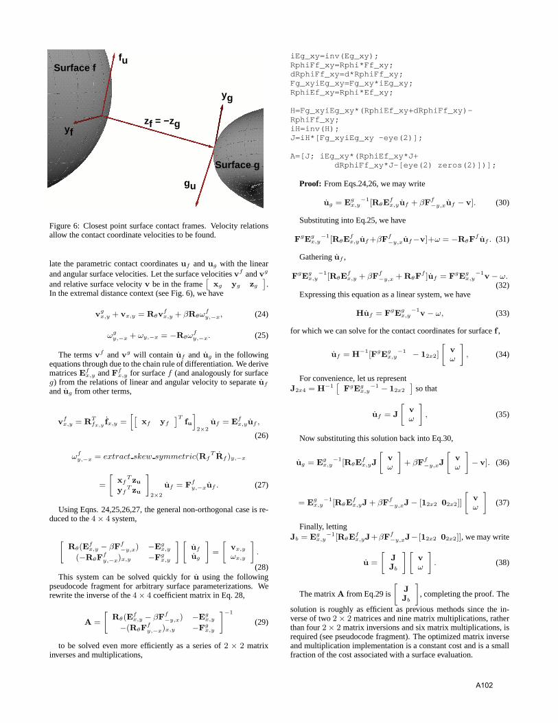
fuSurface f
yfzf = −zg
gu
yg
Surface g
Figure 6: Closest point surface contact frames. Velocity relationsallow the contact coordinate velocities to be found.
late the parametric contact coordinatesuf andug with the linearand angular surface velocities. Let the surface velocitiesvf andvg
and relative surface velocityv be in the frame[
xg yg zg
].
In the extremal distance context (see Fig. 6), we have
vgx,y + vx,y = Rθv
fx,y + βRθωf
y,−x, (24)
ωgy,−x + ωy,−x = −Rθω
fy,−x. (25)
The termsvf andvg will contain uf and ug in the followingequations through due to the chain rule of differentiation. We derivematricesEf
x,y andFfx,y for surfacef (and analogously for surface
g) from the relations of linear and angular velocity to separateuf
andug from other terms,
vfx,y = RT
fx,yfx,y =
[[xf yf
]Tfu
]2×2
uf = Efx,yuf ,
(26)
ωfy,−x = extract skew symmetric(Rf
T Rf )y,−x
=
[xf
T zu
yfT zu
]2×2
uf = Ffy,−xuf . (27)
Using Eqns. 24,25,26,27, the general non-orthogonal case is re-duced to the4 × 4 system,
[Rθ(E
fx,y − βFf
−y,x) −Egx,y
(−RθFfy,−x)x,y −Fg
x,y
] [uf
ug
]=
[vx,y
ωx,y
].
(28)This system can be solved quickly foru using the following
pseudocode fragment for arbitrary surface parameterizations. Werewrite the inverse of the4 × 4 coefficient matrix in Eq. 28,
A =
[Rθ(E
fx,y − βFf
−y,x) −Egx,y
−(RθFfy,−x)x,y −Fg
x,y
]−1
(29)
to be solved even more efficiently as a series of2 × 2 matrixinverses and multiplications,
iEg_xy=inv(Eg_xy);RphiFf_xy=Rphi*Ff_xy;dRphiFf_xy=d*RphiFf_xy;Fg_xyiEg_xy=Fg_xy*iEg_xy;RphiEf_xy=Rphi*Ef_xy;
H=Fg_xyiEg_xy*(RphiEf_xy+dRphiFf_xy)-RphiFf_xy;iH=inv(H);J=iH*[Fg_xyiEg_xy -eye(2)];
A=[J; iEg_xy*(RphiEf_xy*J+dRphiFf_xy*J-[eye(2) zeros(2)])];
Proof: From Eqs.24,26, we may write
ug = Egx,y−1[RθE
fx,yuf + βFf
−y,xuf − v]. (30)
Substituting into Eq.25, we have
FgEgx,y−1[RθE
fx,yuf +βFf
−y,xuf−v]+ω = −RθFf uf . (31)
Gatheringuf ,
FgEgx,y−1[RθE
fx,y + βFf
−y,x + RθFf ]uf = FgEg
x,y−1v − ω.
(32)Expressing this equation as a linear system, we have
Huf = FgEgx,y−1v − ω, (33)
for which we can solve for the contact coordinates for surfacef ,
uf = H−1[FgEgx,y−1 − 12x2]
[vω
], (34)
For convenience, let us representJ2x4 = H−1
[FgEg
x,y−1 − 12x2
]so that
uf = J
[vω
], (35)
Now substituting this solution back into Eq.30,
ug = Egx,y−1[RθE
fx,yJ
[vω
]+ βFf
−y,xJ
[vω
]− v]. (36)
= Egx,y−1[RθE
fx,yJ + βFf
−y,xJ− [12x2 02x2]]
[vω
](37)
Finally, lettingJb = Eg
x,y−1[RθE
fx,yJ+βFf
−y,xJ− [12x2 02x2]], we may write
u =
[JJb
][vω
]. (38)
The matrixA from Eq.29 is
[JJb
], completing the proof. The
solution is roughly as efficient as previous methods since the in-verse of two2 × 2 matrices and nine matrix multiplications, ratherthan four2 × 2 matrix inversions and six matrix multiplications, isrequired (see pseudocode fragment). The optimized matrix inverseand multiplication implementation is a constant cost and is a smallfraction of the cost associated with a surface evaluation.
A102

7.2 Cartesian and Quaternion Generalized Veloci-ties
Now we express the relative surface velocities in terms of worldframe body coordinate velocities so that integration of orientationis possible (integration of angular velocity is meaningless). Definethe local contact frame through the rotation matrix
Rloc =[
xg yg zg
]T. (39)
Let Gf = G(qf,rot), Gg = G(qg,rot), whereG(qrot) is thematrix operator mapping quaternion velocities to angular velocities[Haug, 1992, Shabana, 1998], given by
G(qrot) = 2
[ −qrot2 qrot1 qrot4 −qrot3−qrot3 −qrot4 qrot1 qrot2−qrot4 qrot3 −qrot2 qrot1
]. (40)
The velocity[vT ωT ]T is the motion of surfaceg relative to sur-facef . We write our world space velocities in terms of the localframe. We relate relative angular velocity and world frame quater-nion velocity by
ω = Rloc
[ −TfGf TgGg
] [qf,rot
qg,rot
], (41)
and relative linear velocity to Cartesian velocity through
v = Rloc(qg,tr − qf,tr + (ωglg − ωgl
f )× (g(u)− qg,tr)). (42)
× denotes the vector cross product.Tf and Tg are rota-tions from the local frame to the world frame defined by quater-nionsqf,rot andqg,rot. We write the relative surface velocities[vT , ωT ]T as[
vω
]=
[Rloc −Rloc(g(u) − qg,tr)×0 Rloc
]∗
[−I3x3 03x4 I3x3 03x4
03x3 −2TfGf 03x3 2TgGg
] [qf
qg
](43)
where× in Eq. 43 denotes the3x3 skew symmetric matrix thatperforms the operation of a cross product (obtained from the three
components of a vector, i.e.a× =[
0 −az ayaz 0 −ax−ay ax 0
]). From
Eq. 38, the truncated part[vTx,y, ωT
x,y]T is all that is required. LetB contain the first two rows and rows four and five of Eq. 43. Sub-stituting[vT
x,y, ωTx,y]T into Eq. 38, yields
u = AB
[qf
qg
]. (44)
7.3 Non-Orthogonal Surface-Curve Velocity For-mulation
Similarly, it may be shown that the surface-curve extremal distanceequations may be extended to for arbitrary surface parameteriza-tions.
The time derivative of the parametric contact coordinates for sur-facef and curveg may be written as a function of linear and angularvelocity multiplying a matrix operator,
u3x1 =
[Rθ(E
fu + dFf
x,y) −gux,y
−RθFfx,y −kgsin(φ)gux,y
]−1
3x3
[vx,y
ωy
]3x1
,
(45)
where
kg =||gu × guu||
||gu||3 (46)
andφ is the angle between the curve normal (which is−zf forthe extremal distance case) and the curve binormalb, about thecurve x axisgu. The binormal is
b =gu × guu
||gu × guu|| . (47)
Eq. 43 is again used to establish this relation in terms of quater-nion and Cartesian velocities, using rows 1,2, and 5.
References
[Bajaj, 1988] Bajaj, C., Hoffmann, C., Lynch, R., Hopcroft, J.,“Tracing surface intersections,” inComputer Aided GeometricDesign, Vol 5, 1988, pp. 285-307.
[Baraff, 1990] Baraff, D., “Curved surfaces and coherence for non-penetrating rigid body simulation”, inComputer Graphics Pro-ceedings, SIGGRAPH, 24(4): 19-28, 1990.
[Cai, 1987] Cai, C., Roth, B., “On the spatial motion of rigid bod-ies with point contact,” inInternational Conference on Roboticsand Automation,pp. 686-695, March 1987.
[Cameron, 1997] Cameron, S., “Enhancing GFK: ComputingMinimum and Penetration Distances between Convex Polyhe-dra,” in International Conference on Robotics and Automation,April 1997.
[Cremer, 1996] Anitescu, M., Cremer, J., and Potra, F., “Formu-lating 3D Contact Dynamics Problems,”Mech. Struct. & Mach.,vol. 24, no. 4, pp. 405-437, Nov. 1996.
[Cohen, 1980] Cohen, E., Lyche, T., and Riesenfeld, R., “DiscreteB-Splines And Subdivision Techniques In Computer Aided Ge-ometric Design And Computer Graphics,”Computer Graphicsand Image Processing,Vol 14, Number 2, October 1980.
[De, 1998] De, S., Srinivasan, M., “Rapid Rendering of”Tool-Tissue” Interactions in Surgical Simulations: ThinWalled Membrane Models”, PHANToM User’s Group Pro-ceedings, PUG 1998, http://www.sensable.com/ community/PUG98papers.htm.
[Gregory, 1998] Gregory, A., Lin, M., Gottschalk, S., Taylor, R.,“H-Collide: A Framework for Fast and Accurate Collision De-tection for Haptic Interaction,” UNC Report, currently unpub-lished, 1998.
[Gilbert, 1988] Gilbert, E., Johnson, D., Keerthi, S. “A Fast Proce-dure for Computing the Distance between Complex Objects inThree-Dimensional Space,” IEEE Journal of Robotics and Au-tomation, pp. 193-203, April 1988.
[Haug, 1992] Haug, E., Intermediate Dynamics, Prentice Hall,1992.
[Johnson, 1998a] Johnson, D. E., and Cohen, E., “ A frameworkfor efficient minimum distance computations,” Proc. IEEE Intl.Conf. Robotics & Automation, Leuven, Belgium, May 16-21,1998, pp. 3678-3684.
A103

[Johnson, 1998b] Johnson, D.E., and Cohen, E., “An improvedmethod for haptic tracing of sculptured surfaces,” Symp. onHaptic Interfaces, ASME International Mechanical EngineeringCongress and Exposition, Anaheim, CA, Nov. 15-20, 1998, inpress.
[Kriezis, 1992] Kriezis, G., Patrikalakis, N., Wolder, F., “Topolog-ical and differential-equation methods for surface intersections,”in Computer-Aided Design,vol. 24, no. 1, January 1992, pp. 41-51.
[Lin, 1994] M.C. Lin, D. Manocha, and J. Canny. Fast contact de-termination in dynamic environments. inIEEE Conference onRobotics and Automation,pp. 602-609, 1994.
[Maekawa, 1996] Maekawa, T., Wolter, F., Patrikalakis, N., “Um-bilics and lines of curvature for shape interrogation,” inCom-puter Aided Geometric Design,vol. 13, no. 2, March 1996.
[McCalla, 1967] McCalla, T., Introduction to Numerical Methodsand FORTRAN Programming, John Wiley & Sons, Inc., 1967.
[Montana, 1986] Montana, D., J., 1986, Tactile sensing and thekinematics of contact, Ph.D. Thesis, Division of Applied Sci-ences, Harvard University.
[Montana, 1988] Montana, D., “The Kinematics of Contact andGrasp”, inInt. J. of Rob. Res.,vol. 7, no. 3, June 1988.
[Murray, 1990] Murray, R., Robotic Control and NonholonomicMotion Planning, PhD. Dissertation, Electronics Research Lab-oratory, College of Engineering, University of California, Berke-ley, 1990.
[NRC, 1995] National Research Council, Virtual Reality: Scien-tific and Technological Challenges, Committee on Virtual Real-ity Research and Development, National Academy Pres, 1995,p.69.
[Quinlan, 1994] Quinlan, S. “Efficient Distance Computation be-tween Non-Convex Objects,” IEEE Int. Conference on Roboticsand Automation, pp. 3324-3329, 1994.
[Ruspini, 1997] Ruspini, D., Kolarov, K., Khatib, O., “The Hap-tic Display of Complex Graphical Environments,” inComputerGraphics Proceedings, SIGGRAPH,August, 1997.
[Ruspini, 1998] Ruspini, D., Khatib, O., “Dynamic Models forHaptic Rendering Systems.” inAdvances in Robot Kinematics:ARK’98, June 1998, Strobl/Salzburg, Austria, pp 523-532.
[Sato, 1996] Sato, Y., Hirata M., Maruyama T., Arita Y., “Effi-cient Collision Detection using Fast Distance Calculation: Al-gorithms for Convex and Non-Convex Objects,” inProceedingsof the 1996 IEEE International Conference on Robotics and Au-tomation,April, 1996, pp. 771-778.
[Shabana, 1998] Shabana, A., Dynamics of Multibody Systems,Cambridge University Press, 1998.
[Stewart, 1997] Stewart P., Chen Y., Buttolo P., “CAD Data Rep-resentations for Haptics Virtual Prototyping,” inProceedings ofDETC ’97, 1997 ASME Design Engineering Technical Confer-ences, Sept. 14-17, 1997, Sacramento, CA.
[Snyder, 1995] Snyder, J., “An Interactive Tool for Placing CurvedSurfaces without Interpenetration,” inComputer Graphics Pro-ceedings, SIGGRAPH,Los Angeles, August 6-11, 1995, pp.209-216.
[Thompson, 1997] Thompson II, T.V., Nelson, D.D., Cohen, E.,and Hollerbach, J.M., “Maneuverable NURBS models within ahaptic virtual environment,”6th Annual Symp. Haptic Interfacesfor Virtual Environment and Teleoperator Systems,DSC-Vol. 61,(Dallas, TX), pp. 37-44, Nov. 15-21, 1997.
[Thompson, 1999] Thompson II, T.V., Cohen, E., “DIRECT HAP-TIC RENDERING OF COMPLEX TRIMMED NURBS MOD-ELS,” in 8th Annual Symp. Haptic Interfaces for Virtual Envi-ronment and Teleoperator Systems,(Nashville, TN), 1999.
[Zilles, 1995] Zilles, C.B., and Salisbury, J.K., “A Constraint-based God-object Method For Haptic Display,” inProc. IEE/RSJInternational Conference on Intelligent Robots and Systems, Hu-man Robot Interaction, and Cooperative Robots,Vol 3, pp. 146-151, 1995.
A104

A105

A106
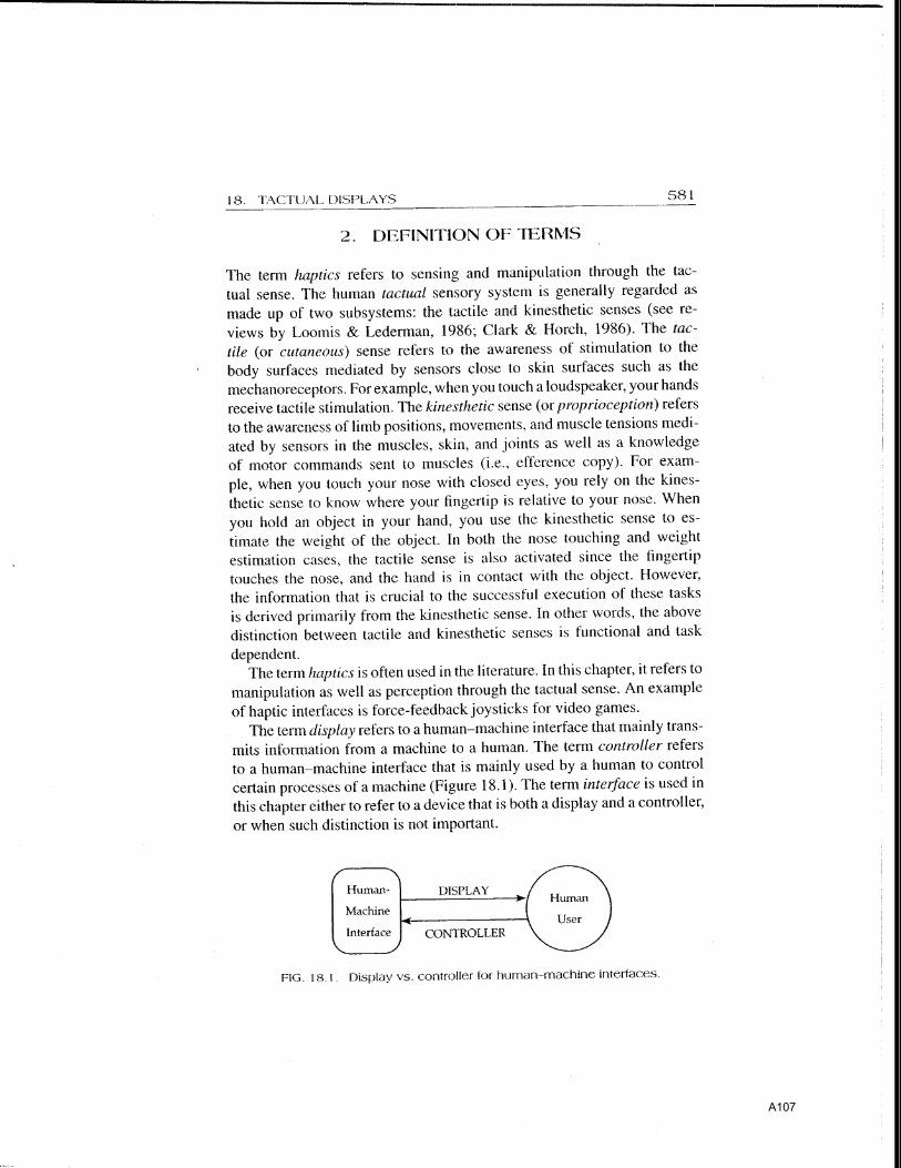
A107
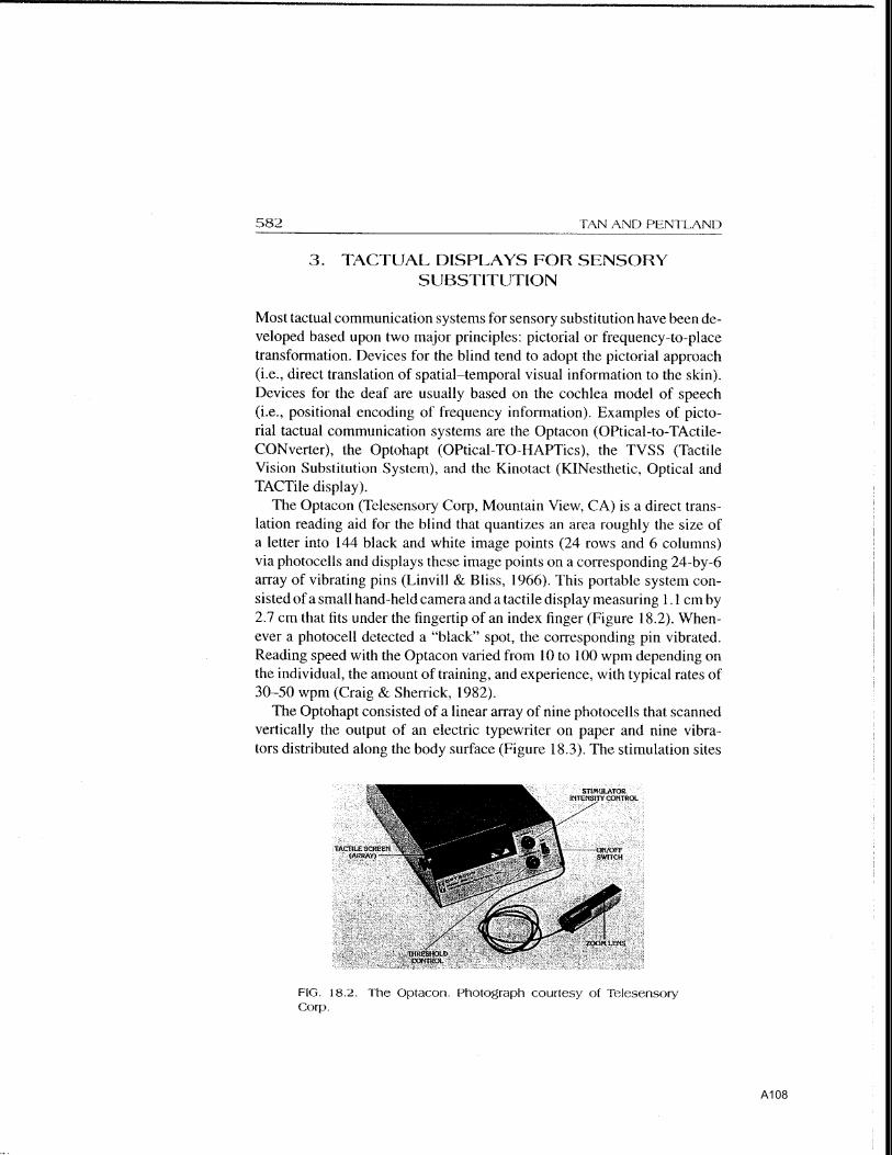
A108

A109

A110

A111

A112

A113

A114

A115

A116

A117

A118

A119

A120

A121

A122

A123

A124

The emerging science of haptic renderingconsists of delivering properties of phys-
ical objects through the sense of touch. Owing to therecent development of sophisticated haptic-renderingalgorithms, users can now experience virtual objectsthrough touch in many exciting applications, includingsurgical simulations, virtual prototyping, and data per-ceptualization. Haptics holds great promise to enrichthe sensory attributes of virtual objects that these sys-tems can produce.
One area that has received increas-ing attention in the haptics commu-nity is haptic texture rendering, thegoal of which is to introduce micro-geometry-scale features on objectsurfaces. Haptic objects renderedwithout textures usually feel smooth,and sometimes slippery. Appropriatehaptic textures superimposed on hap-tic objects enhance an object’s real-ism. For example, we can make thesame cubic structure feel like a brickwith rough surface textures or a card-board carton with finer textures.Clearly, haptic texture rendering is anexciting research field that can takehaptic rendering to the next level.
Although much effort has beendevoted to haptic texture rendering—mostly in model-ing and rendering techniques1,2—the research commu-nity must overcome many challenges before haptictexture rendering can be widely used in real applications.One common problem in haptically rendered textures isthat they are sometimes perceived to behave unrealisti-cally, for example, by buzzing or by the apparent alive-ness of a textured surface. Due to the complex nature ofthe haptic-rendering pipeline and the human somatosen-sory system, it remains a difficult problem to expose allfactors contributing to such perceptual artifacts.
At the Haptic Interface Research Laboratory at Pur-due University, we are among the first to have system-atically investigated the unrealistic behavior of virtual
haptic textures. This article presents a summary of ourrecent work in this area. We hope this article will stim-ulate further discussion among haptics researchers andapplications developers who are interested in haptic tex-ture rendering. Interested readers may refer to our pre-vious publications for more details.3-7
Perceived instabilityWe use the term perceived instability to refer to all unre-
alistic sensations—such as buzzing—that cannot beattributed to the physical properties of a textured sur-face being rendered with a force-feedback device. Todevelop haptic texture-rendering models and methodsthat can deliver realistic textures to human users, youmust understand the conditions under which texturedvirtual objects are free of perceptual artifacts, and youmust also recognize the sources of perceived instabili-ties. We developed the notion of perceived instability toinclude the effects of all factors in haptic interaction thatcan result in unrealistic sensations. As shown in Figure 1,haptic interaction occurs at a haptic interaction tool thatmechanically connects two symmetric dynamic systems.In principle, each block in the diagram can contribute tothe perception of instability by the human user.
A crucial difference between real and virtual hapticinteractions with an object is that a virtual environmentimparts no haptic sensation to the user unless the inter-action tool penetrates the object surface. The first phaseof haptic texture rendering is the computation of the pen-etration depth and the resulting force command using ahaptic texture renderer stored in the computer. For thispurpose, most haptic systems repeat several proceduresat a high update rate, usually 1 KHz or higher. First, thesystem measures the position of the haptic interactiontool using position sensors embedded in the haptic inter-face. The system then compares the measured positionof the interaction tool with the location of objects in thevirtual environment. If the interaction tool penetrates thesurface of any virtual object, a response force is comput-ed and sent to the haptic interface to create the intendedhaptic effect. Finally, if the state of any virtual object haschanged due to the interaction, the system updates the
Haptic Rendering—Beyond Visual Computing
New sophisticated haptic-
rendering algorithms let
users experience virtual
objects through touch. The
authors systematically
investigate the unrealistic
behavior of virtual haptic
textures.
Seungmoon Choi and Hong Z. TanPurdue University
Toward RealisticHaptic Renderingof Surface Textures
40 March/April 2004 Published by the IEEE Computer Society 0272-1716/04/$20.00 © 2004 IEEEA125

database of virtual objects.Two of these four steps—collision
detection and response force com-putation—can have a significanteffect on perceived instability. Thesetwo steps determine the so-calledenvironment dynamics, the reactiondynamics of the haptic renderer to auser input. In most cases, the envi-ronment dynamics is an approxima-tion of the corresponding real-worldcontact dynamics because simulat-ing the actual physics is usually toocomplex to accomplish in real time. The simplified envi-ronment dynamics must preserve the essence of the realcontact dynamics to produce sensations consistent witha user’s experience and expectation. Otherwise, the userperceives unrealistic behaviors of haptically renderedobjects, and perceived instability occurs. This issue hasreceived little attention from the research communitybecause a majority of studies on haptic texture render-ing have focused on the development of time-efficientrendering algorithms.
The next phase of haptic texture rendering is the deliv-ery of force to the human user. During this process, theforce-feedback device must remain stable to avoid per-ceived instability. Device instability, such as mechanicalresonance, can result in force variations in addition tothe force command received from the haptic texture ren-derer. In our experiences, a user usually judges the hap-tically rendered textured surface as unstable when anextraneous signal—such as high-frequency buzzing—occurs from the haptic interface. This issue has receivedmuch attention in the context of control engineering,although most studies assume a much simpler virtualenvironment such as a flat wall without any textures.8
Much work is needed to extend the techniques for solv-ing the hard-wall stability problem.
The last phase of haptic texture rendering is the per-ception of force by a human user. The human user sens-es the mechanical stimuli from the haptic interface,extracts information from force variations, forms a per-cept of the virtual object being rendered, and determineswhether the virtual object is realistic. To determinewhether the user perceives instability from a textured sur-face rendered by the haptic interface, we must resort topsychophysical studies. Psychophysics is a branch of psy-chology with well-developed methodology for studyingthe relation between geometrical and physical propertiesof objects and the percept. At this point, little knowledgeis available in the literature on the perceived instabilityof haptically rendered objects, because this is a newresearch topic that has only become relevant with therecent capability to render haptic virtual environments.
Goals and approachesOur long-term goal is to develop haptic texture-ren-
dering systems that deliver realistic sensations of virtu-al haptic textures. To do so requires the appropriatedesign of a texture renderer, the stable control of a hap-tic interface, and a better understanding of thesomatosensory system. As a first step, our research has
focused on understanding the nature of perceived insta-bility. Specifically, we
investigated the conditions under which perceivedinstability of virtual textures occurs,
discovered the types of perceived instability fre-quently reported by human users,
identified the proximal stimuli that contributed to theperception of instability, and
unveiled the sources that produced the stimuli.
We conducted psychophysical experiments to quanti-fy the conditions under which users perceived instabili-ty from virtual textures and to understand the associatedpercept. We also measured the physical stimuli deliveredby the haptic interaction tool to the user’s hand under var-ious conditions where the textures were perceived to bestable and unstable. By analyzing the measured data, welocated signal components responsible for the perceptionof instability. We achieved the last goal by investigatingwhich component in the haptic texture-rendering systemgenerated the signals that led to perceived instability.
Because of the plethora of texture-rendering modelsand methods, we chose a benchmark consisting of themost essential features common to many texture-ren-dering systems for studying perceived instability. Inaddition, we had to consider the effect of user explo-ration patterns because the user is mechanically cou-pled to the haptic interface. For the apparatus, we useda Phantom force-reflecting device (from SensAble Tech-nologies) shown in Figure 2. This is the most widely useddevice for haptics research and applications.
IEEE Computer Graphics and Applications 41
BrainComputer
A ctuation
PerceptionSensing
Action
Haptic rendering system Human user
Sensorimotorsystem
Interactiontool
Hapticinterface
Mechanically coupled
1 Illustration of the key components of the interaction between a haptic rendering system anda human user.
z
xy
Accelerometer
p(t)
World coordinate frame
Force/torquesensor
2 Phantom1.0A used in ourstudies. This is amodified Phan-tom instrument-ed withadditionalforce-torqueand accelera-tion sensors.
A126

For the texture model, we used a 1D sinusoidal grat-ing superimposed on a flat surface (see Figure 3). Thegrating is represented by
in the Phantom world coordinate frame where A and Lare the amplitude and wavelength of the grating. Sinu-soidal gratings have been widely used as basic buildingblocks for textured surfaces in studies on haptic textureperception and as a basis function set for modeling realhaptic textures.
For collision detection, we used two methods of com-puting penetration depth d(t):
and
where p(t) = (px(t), py(t), pz(t)) was the position of thePhantom stylus tip and h(px(t)) = Asin (2π/L px(t)) + Awas the height of the textured surface at px(t). The firstmethod, d1(t), assumed that collision detection wasbased on the plane underlying the textured surface (z =0). The advantage of d1(t) was that we can easily gen-eralize it to textured objects with a large number ofunderlying polygons because the plane could representa face on a polygon. The disadvantage was that it intro-duced discontinuity in computed penetration depth(and subsequently in response force) when the Phan-tom stylus entered and left the textured surfaces.
The second method d2(t) declared a collision as soonas the stylus entered the texture boundary. The advan-tage of this method was that it ensured a continuous
change in computed penetration depth and responseforce. The disadvantage was that it’s much more diffi-cult to apply this algorithm to textured polygonal objectsfor two reasons. One is the nonlinearity associated withthe representation of textured object surfaces that usu-ally requires iterative numerical algorithms for collisiondetection. The other is the lack of a global representationof the boundaries of the textured virtual objects. In atypical implementation, the polygons and the texturemodel are stored separately, and the texture model islocally mapped onto a point on the polygon whenevernecessary. It’s often infeasible to do a global collisiondetection using only the local information. To the bestof our knowledge, the application of the collision detec-tion method based on d2(t) to a general class of texturedobjects is still an open research issue.
We employed two basic texture-rendering methods.Both used a spring model to calculate the magnitude ofrendered force, but they differed in the way they ren-dered force directions. Force magnitudes were calcu-lated as K ⋅ d(t), where K was the stiffness of the texturedsurface and d(t) was the penetration depth of the stylusat time t (see Figure 3). In terms of force directions, thefirst method rendered a force Fmag(t) with a constantdirection normal to the flat wall underlying the texturedsurface. The second method rendered a force Fvec(t) withvarying direction such that it remained normal to thelocal microgeometry of the sinusoidal texture model.Mathematically, Fmag(t) = Kd(t)nw, and Fvec(t) =Kd(t)nT(p(t)), where nw was the normal vector of theunderlying flat wall, and nT(p(t)) was the normal vec-tor of the textured surface at p(t). Both methods keptthe force vectors in horizontal planes, thereby mini-mizing the effect of gravity on rendered forces.
The two texture-rendering methods are naturalextensions of virtual wall rendering techniques. Per-ceptually, they are very different: Textures rendered byFvec(t) feel rougher than those rendered by Fmag(t) forthe same texture model. Textures rendered by Fvec(t)also feel sticky sometimes.
Our exploration mode refers to a stereotypical pat-tern of the motions that a user employs to perceive a cer-tain attribute of objects through haptic interaction. Wetested two exploration modes—free exploration andstroking. In the free exploration mode, users coulddetermine and use the interaction pattern that was mosteffective at discovering the instability of the renderedtextures. We selected this mode as the most challeng-ing interaction pattern for a haptic texture renderingsystem in terms of perceived stability. With the strokingmode, users should move the stylus laterally across thetextured surfaces. We chose this mode to be represen-tative of the typical and preferred exploration patternfor accurate texture perception.9
We conducted psychophysical experiments to quanti-fy the parameter space within which textures were per-ceived as stable and to categorize the types of perceivedinstability discovered by users. We employed the methodof limits, a well-established classical psychophysicalmethod, in all our experiments.10 And we employed adiverse range of experimental conditions, with factorsincluding texture model parameter (amplitude and wave-
d t
p t h p t
AL
p t A p t p t h
z x
x z z2
0
2( )
( ) ( )
( ) ( ) ( )=
> ( )
+ − ≤
if
sin ifπ
pp tx( )( )
d t
p t
AL
p t A p t p t
z
x z z1
0 0
20
( )
( )
( ) ( ) ( )=
>
+ − ≤
if
sin ifπ
z AL
x A=
+sin2π
Haptic Rendering—Beyond Visual Computing
42 March/April 2004
x
z
yPenetration depth: d(t)
z = 0
Stylus tip: p(t) = (px(t), py(t), pz(t))
z = Asin(––– x) + A2πL
nW
nT (p(t))
3 Illustration of the texture rendering models and methods used in ourstudies.
A127

length of the 1D sinusoidal gratings), texture renderingmethod, exploration mode, and collision-detectionmethod. In each experimental condition, a subject’s taskwas to explore a virtual textured plane rendered withPhantom and to decide whether the textured plane exhib-ited any perceived instability. The dependent variablemeasured in the experiments was the maximum stiffnessKT under which the rendered textured plane did not con-tain any perceived instability. A more detailed descrip-tion of experiment design can be found elsewhere.3,4,6
We measured physical stimuli to isolate the signalsresponsible for the perception of instability and to iden-tify their sources. For this purpose, we added two moresensors—6D force-torque sensor and 3D accelerome-ter—to the Phantom, as shown in Figure 2, and mea-sured the nine associated physical variables—3Dposition, 3D force, and 3D acceleration—that were deliv-ered to a user’s hand. We collected data for many exper-imental conditions on the basis of the parameter spaceobtained from the psychophysical experiments. By com-paring the measured data of both perceptually stable andunstable cases in the time and frequency domains, weisolated the physical stimuli that induced the perceptionof instability. We also investigated the sources for thesesignals using additional hypothesis-driven experiments.
Parameter spacesFigure 4 shows an example of a parameter space for
perceptually stable haptic texture rendering based ondata obtained from the psychophysical experiments. Wemeasured the data when the subject stroked virtual tex-tures rendered with d1(t) (collision detection based onthe plane underlying the textured surface) and Fvec(t)(variable force directions). In the figure, A and L repre-sent the amplitude and wavelength of the sinusoidaltexture model, respectively, and KT denotes the maxi-mum stiffness value under which a virtual texture feltstable. The blue rectangles in the figure represent thestiffness thresholds averaged over three subjects for thecorresponding texture model parameters. Also shownis a best-fit surface to the measured data found byregression analysis. The region under the mesh surfacerepresents the parameter space of (A, L, K) for percep-tually stable haptic texture rendering, and the regionabove the mesh surface contains parameters that resultin virtual textures that were perceived as unstable.
The most significant result of the psychophysicalexperiments was that the parameter spaces for percep-tually stable texture rendering were limited. See Table1 for a summary. Under most experimental conditions,the virtual textures that could be rendered without any
IEEE Computer Graphics and Applications 43
0.5
1
1.5
21
2
3
4
0
0.1
0.2
0.3
0.4
0.5
0.6
L (mm)
A (mm)
K T (
N/m
m) 4 Example of
psychophysicalresults.
Table 1. Average stiffness thresholds for perceptually stable texture rendering.
d1(t) d2(t) Experiments Range (N/mm) Mean (N/mm) Range (N/mm) Mean (N/mm)
Fmag(t), free exploration 0.0586 – 0.1023 0.0799 0.1813 – 0.5383 0.3486Fmag(t), stroking 0.4488 – 0.1664 0.3116 0.2490 – 0.6410 0.3603Fvec(t), free exploration 0.0097 – 0.0367 0.0209 0.0181 – 0.0260 0.0235Fvec(t), stroking 0.0718 – 0.3292 0.1848 0.3254 – 0.4638 0.3808
A128

perceived instability felt soft—similar to the feel of cor-duroy. Textures rendered with higher stiffness valuesusually contained unrealistic sensations, such asbuzzing and aliveness. For the haptic texture renderingsystem used in our experiments to be useful for gener-ating a large range of textures, we need to enlarge theparameter spaces for perceptually stable rendering.
We examined the effects of experiment factors—tex-ture model parameters, collision detection method, tex-ture rendering method, and exploration mode—byapplying statistical analysis on the psychophysicalresults. In general, stiffness thresholds tended toincrease when the amplitude of the sinusoidal texturemodel decreased or when the wavelength increased.Collision detection method d2(t) resulted in larger stiff-ness thresholds than d1(t), except for experiments usingFvec(t) and free exploration where the thresholds weretoo small to exhibit any trends (see Table 1). In mostcases, textures rendered with Fmag(t) (constant forcedirection) showed larger stiffness thresholds than thosewith Fvec(t) (variable force direction). On average, tex-tures explored by stroking resulted in larger stiffnessthresholds than those by free exploration.
To gain insight into the effects of texture model para-meters on perceived instability, we consider the deriva-tive of force magnitude. Let g(t) = |Fmag(t)| = |Fvec(t)|denote force magnitude, and assume that the stylus isin contact with the textured surface. From there we have
Differentiating g(t) with respect to the time variablet results in
(1)
There are two terms in Equation 1 that determine therate of change of force magnitude. The term on the right,Kpz(t), responds to stylus velocity in the normal direc-tion to the underlying plane pz(t) with a gain of K. Theterm on the left is due to the virtual textures. Here, thelateral velocity of the stylus px(t) is amplified with threeconstant gains (K, A, and 1/L) and one variable gain thatdepends on the lateral position of the stylus px(t).Increasing A or decreasing L results in a faster changein force magnitude which can cause a textured surfaceto be perceived as less stable, or equivalently, result in asmaller stiffness threshold KT.
We expected that d2(t) would generate perceptuallymore stable textures than d1(t) because it removed dis-continuities in force commands at the texture entrypoints. This expectation was confirmed, except for thecondition where the subjects freely explored the virtu-al haptic textures rendered with Fvec(t). The stiffnessthresholds measured using Fvec(t) and free explorationwere practically zero for both d1(t) and d2(t), and hencedid not exhibit any significant trend. The reason that thetextures felt unstable was the presence of strong buzzingnoises whenever we positioned the Phantom stylus deep
inside the textured surfaces.Our finding that textures rendered with Fmag(t) result-
ed in larger stiffness thresholds than those rendered withFvec(t) was also consistent with the nature of these tworendering methods. While Fmag(t) imposed perturbationsin the force magnitude only, Fvec(t) resulted in perturba-tions in the force direction as well as force magnitude.The sometimes abrupt changes in force direction couldcause virtual textures rendered with Fvec(t) to be per-ceived as less stable than those rendered with Fmag(t).Perceptually, Fvec(t) is a useful rendering method becauseit can produce textures that feel much rougher than thoserendered with Fmag(t) using the same texture model.
We expected the experimentally confirmed fact thatstroking would result in a larger stiffness threshold thanfree exploration for the same rendering parameters. Oursubjects rarely used stroking in the free explorationmode although it was allowed. Instead, they chose toposition the stylus at various locations on or inside thevirtual textured surface to focus on the detection of per-ceived instability. Therefore, in the free explorationmode, the subjects concentrated on the detection ofunrealistic vibrations in the absence of any other sig-nals. In the stroking mode, the subjects always felt thevibrations due to the stylus stroking the virtual texturedsurface. They had to detect additional noise to declarethe textured surface as unstable. Due to possible mask-ing of the different vibrations coming from the texturedsurface, it’s conceivable that subjects could not detectinstability with stroking as easily as they would with sta-tic positioning of the stylus. Indeed, our subjects report-ed that the experiments with stroking were moredifficult to perform.
Frequently observed perceivedinstabilities
We found three types of frequently reported perceivedinstability in the psychophysical experiments: buzzing,aliveness, and ridge instability. The first two relate tothe perception of force magnitude, while the otherrelates to the perception of force direction. Buzzingrefers to high-frequency vibrations that subjects felt atthe Phantom stylus when it touched virtual textured sur-faces. We observed this type of perceived instability inmost experimental conditions, particularly when thestiffness values were much higher than the thresholdsmeasured in the psychophysical experiments. The sub-jects reported that buzzing appears to be of higher fre-quencies than the vibrations induced by the stroking ofvirtual textures.
Measurement data supported the anecdotal report.Whenever the subjects felt buzzing, spectral componentsin a high-frequency region (roughly 150 to 250 Hz)appeared in the power spectral densities of the vibrationstransmitted through the stylus. An example is shown inFigure 5. In this figure, the horizontal axis represents fre-quency from 10 to 500 Hz, while the vertical axis showsthe power spectrum density of pz(t) (the measured sty-lus position along the normal direction of the texturedplane) in dB relative to 1-micrometer peak sinusoidalmotion. We can observe a spectral peak at around 71 Hz.Additional prominent spectral peaks appear in the high
& & &g tKAL L
p t p t Kp tx x z( ) cos ( ) ( ) ( )=
−22
ππ
g t K AL
p t A p tx z( ) sin ( ) ( )=
+ −
2π
Haptic Rendering—Beyond Visual Computing
44 March/April 2004A129

frequency region starting at around150 Hz. The intensities of the high-frequency vibrations are up to 25 dBabove the human detection thresh-olds at the corresponding frequency(the red dotted line). These high-fre-quency spectral peaks caused thebuzzing.
We suspected that the rapidlychanging force commands for tex-ture rendering might have excitedthe high-frequency dynamics of thePhantom, thereby causing high-fre-quency vibration to be transmittedthrough the stylus. We thereforemeasured the frequency responseof the Phantom near the origin of itsworld coordinate frame and foundthat the Phantom indeed exhibiteda mechanical resonance at 218 Hz.This resonance was likely the sourceof the high-frequency spectralpeaks that invoked the perceptionof buzzing.
The second type of instability thatthe subjects frequently observedwas aliveness. It occurred when thePhantom stylus was apparently heldstill yet the subject felt pulsatingforce changes emanating from thetextured surface. The sensationappeared to be at a lower frequencythan that of buzzing. Aliveness wasreported for textures rendered withFmag(t) (fixed force-direction) usingd2(t) as penetration depth (contin-uously varying force commands).The measured physical characteris-tics of perceived aliveness were dif-ferent from those of buzzing.Analyses in the frequency domain shed little insight onthe signals responsible for the percept of aliveness. How-ever, examination of data in the time domain revealedmany instances where perceptible changes in forceoccurred while the stylus was perceived to be station-ary in space along the direction of the force changes.
In Figure 6, the two horizontal axes indicate positionnormal to the textured surface pz(t) and along the later-al stroking direction px(t). The vertical axis shows forcesfelt by the subject’s hand. The duration of the data set is400 ms. The large change in px(t) was the result of thesubject stroking the textured surface. In contrast, therewas little change in pz(t). The change in force was on theorder of 0.5 Newtons. As a result, the subject felt a notice-able change in normal force although the stylus was per-ceived to be barely moving into the textured surface.Therefore, the force variation was interpreted as comingfrom an alive textured surface. Indeed, subjects some-times referred to the virtual object as a pulsating texturedsurface. These observations suggest that aliveness wascaused by larger-than-expected force variations in spite ofposition changes that were barely perceivable.
We suspected that, unlike buzzing, which was causedby unstable control of haptic interface, aliveness wasprobably caused by inaccurate environment dynamics.To investigate this hypothesis, we examined whether itwas possible for a user to perceive aliveness while thetexture-rendering system including the force-feedbackdevice was stable in the control sense. We applied a pas-sivity-based control theory to data measured from a userinteracting with virtual textured surfaces. You canregard a dynamic system as passive if it preserves or dis-sipates its initial energy despite its interaction with anexternal system. Because passivity is a sufficient condi-tion for control stability,8 our hypothesis could be con-firmed if we found cases in which a user perceivedaliveness from a passive texture rendering system.
Using a passivity observer—an online observer formonitoring the energy flow of a dynamic system—weconfirmed that aliveness perception could indeed occurwhen the haptic texture-rendering system was passiveand stable. An example is shown in Figure 7. In this fig-ure, the top panel shows the position data along the lat-eral stroking direction px(t), the second panel shows the
IEEE Computer Graphics and Applications 45
−20
0
20
40
60
Frequency (Hz)
|Pz(
f)|(
dB r
elat
ive
to 1
-µm
pea
k)
Power spectral density of Pz(t)
Human detection thresholds
101 ftex fins102
5 Frequency domain analysis of the signals responsible for buzzing.
−20−10
010
20
− 20
−10
0
10
20 −0.5
−0.25
0
0.25
0.5
pz(t) (mm)px(t) (mm)
FzS
(t)
(N)
F zS (t))(pz(t),F z
S (t))(px(t),
F zS (t))(px(t), pz(t),
(px(t), pz(t))
6 Analysis of aliveness perception in the time domain. Fsz(t) denotes the force measured along
the long axis of the styles.
A130

position variable in the normal direction pz(t), the thirdpanel shows the force along the normal direction Fz
W(t),and the bottom panel shows the values of the passivityobserver. We can see that despite the abrupt forcechanges that resulted in the perception of aliveness, thepassivity observer remained positive. These results pro-vide unequivocal evidence that perceived instability canoccur even when a haptic texture-rendering system ispassive and stable. We have therefore shown indirectlythat environment modeling and human perception canalso play important roles in perceived quality of a hap-tic texture-rendering system.
Consider the difference between touching a real and avirtual surface. When a stylus touches a real surface, it’seither on or off the surface, but not inside the surface.When a stylus touches a virtual surface, however, the sty-lus must penetrate the virtual surface for the user to forma perception of that surface through the resultant forcevariations. With a real surface, a stylus resting on the sur-face can remain stationary. With a virtual surface, how-ever, the stylus’s position can fluctuate inside the surfaceand this fluctuation is amplified to result in perceivable
force variations by a texture render-er, thereby contributing to the per-ception of aliveness. It is well knownthat humans tend to rely more onvision for position-movement infor-mation, and that we can easily inte-grate visual position informationwith haptic force information. Ourrelatively poor kinesthetic resolutionof unsupported hand movements infree space—combined with our rela-tively high sensitivity to forcechanges—is also responsible for theperception of aliveness.
The last type of perceived insta-bility, called ridge instability, is dif-ferent from the first two types in thesense that it is related to the percep-tion of force directions. We use theterm ridge instability to refer to thephenomenon that the Phantom sty-lus was actively pushed to the valleysof the virtual textures rendered withFvec(t) when the stylus was placed onthe ridges of the textures. When a
real stylus rests on the ridge of a real surface with sinu-soidal gratings, the reaction force and friction of the sur-face combine to counterbalance the force exerted by theuser’s hand holding the stylus, thereby creating an equi-librium. The force rendered by Fvec(t), however, was sole-ly based on the local texture geometry and did not takeinto account the direction of user-applied force, as illus-trated in Figure 8. In this figure, we assume that the forceapplied by the user was normal to the plane underneaththe texture. According to the environment model Fvec(t),the force applied by the Phantom was always in the direc-tion of the surface normal nT(p(t)). As a result, the netforce exerted on the tip of the stylus—the sum of theforces applied by the user and the Phantom—was direct-ed toward the valley of the sinusoidal grating. Therefore,the subject who tried to rest the stylus on the ridge couldfeel the stylus being actively pushed into the valley.
ConclusionsIn this article, we have shown that current haptic tex-
ture-rendering systems might suffer from several typesof perceived instability. We also have demonstrated thatperceived instability can come from many sources,including the traditional control instability of hapticinterfaces as well as inaccurate modeling of environ-ment dynamics and the difference in sensitivity to forceand position changes of the human somatosensory sys-tem. Our work underscores the importance of develop-ing texture-rendering algorithms that guarantee theperceptual realism of virtual haptic textures. It is ourhope that this article will encourage more researchers tocontribute to the study of perceived instability of virtu-al haptic textures.
AcknowledgmentsThis work was supported in part by a National Sci-
ence Foundation (NSF) Faculty Early Career Develop-
Haptic Rendering—Beyond Visual Computing
46 March/April 2004
0 2 4 6 8 10 −100
0
100
0 2 4 6 8 10 −5
0
5
0 2 4 6 8 10 −5
0
5
0 2 4 6 8 10 −200
0
200
Time (sec.)
Pass
ivity
obs
erve
r(N
mm
/sec
)F
zW(t
) (N
)p z
(t)
(mm
)p x
(t)
(mm
)
7 Example of using a passivity observer to analyze data corresponding to aliveness perception.Fw
z denotes the force measured along the direction normal to the textured surface.
x
z
y
Stylus orientation nT(p(t))
Phantom response force
Resulting force
User-applied force
Stylus tipp(t)
8 Illustration of the force components involved inridge instability.
A131

ment (CAREER) Award under grant 9984991-IIS and inpart by an NSF award under grant 0098443-IIS. Wethank Blake Hannaford and Jee-Hwan Ryu for discus-sions on the passivity observer. We also thank VincentHayward for discussions on velocity estimation. Thethoughtful comments from the anonymous reviewersare greatly appreciated.
References1. T.H. Massie, Initial Haptic Explorations with the Phantom:
Virtual Touch through Point Interaction, master’s thesis,Dept. of Mechanical Eng., Massachusetts Inst. of Technol-ogy, 1996.
2. C. Ho, C. Basdogan, and M.A. Srinivasan, “Efficient Point-Based Rendering Techniques for Haptic Display of VirtualObjects,” Presence, vol. 8, no. 5, 1999, pp. 477-491.
3. S. Choi and H.Z. Tan, “Perceived Instability of Virtual Hap-tic Texture. I. Experimental Studies,” Presence, 2003, to bepublished.
4. S. Choi and H.Z. Tan, “An Analysis of Perceptual Instabili-ty During Haptic Texture Rendering,” Proc. 10th Int’l Symp.Haptic Interfaces for Virtual Environment and TeleoperatorSystems (IEEE VR 02), IEEE CS Press, 2002, pp. 129-36.
5. S. Choi and H.Z. Tan, “A Study on the Sources of PerceptualInstability During Haptic Texture Rendering,” Proc. IEEEInt’l Conf. Robotics and Automation, IEEE CS Press, 2002,pp. 1261-1268.
6. S. Choi and H.Z. Tan, “An Experimental Study of PerceivedInstability During Haptic Texture Rendering: Effects of Col-lision Detection Algorithm,” Proc. 11th Int’l Symp. HapticInterfaces for Virtual Environment and Teleoperator Systems(IEEE VR 03), IEEE CS Press, 2003, pp. 197-204.
7. S. Choi and H.Z. Tan, “Aliveness: Perceived Instability froma Passive Haptic Texture Rendering System,” Proc.
IEEE/RSJ Int’l Conf. Intelligent Robots and Systems, IEEE CSPress, 2003, pp. 2678-2683.
8. B. Hannaford and J.-H. Ryu, “Time-Domain Passivity Con-trol of Haptic Interfaces,” IEEE Trans. Robotics and Automa-tion, IEEE CS Press, vol. 18, no. 1, 2002, pp. 1-10.
9. S.J. Lederman and R.L. Klatzky, “Hand Movement: A Win-dow into Haptic Object Recognition,” Cognitive Psychology,vol. 19, 1987, pp. 342-368.
10. G.A. Gescheider, Psychophysics: Method, Theory, and Appli-cation, 2nd ed., Lawrence Erlbaum Assoc., 1985.
Seungmoon Choi is a postdoctor-al research associate at the HapticInterface Research Laboratory atPurdue University. His researchinterests include haptic rendering,psychophysics, and robotics. Choireceived a PhD in electrical and com-
puter engineering from Purdue University.
Hong Z. Tan is an associate pro-fessor in the school of electrical andcomputer engineering and the schoolof mechanical engineering (cour-tesy) at Purdue University. Herresearch interests include hapticinterfaces, psychophysics, haptic ren-
dering, and distributed contact sensing. Tan received a PhDin electrical engineering and computer science from theMassachusetts Institute of Technology.
Readers may contact Hong Tan at Purdue Univ., Elec-trical Eng. Building, 465 Northwestern Ave., WestLafayette, IN 47907; [email protected].
IEEE Computer Graphics and Applications 47
ArchitecturesSupport Services
Algorithm/Protocol Design and AnalysisMobile Environment
Mobile Communication SystemsApplications
Emerging Technologies
IEEE Transactions onMobile Computing
revolutionary new quarterly journal that seeks out and delivers the very best peer-reviewed research results on mobility of users, systems, data, computing information organization and access, services, management,
and applications. IEEE Transactions on Mobile Computing gives youremarkable breadth and depth of coverage …
ATo subscribe:
http://computer.org/tmc
or callUSA and CANADA:
+1 800 678 4333WORLDWIDE:
+1 732 981 0060
SubscribeNOW!
A132

Haptic Display of Interaction between Textured Models
Miguel A. Otaduy Nitin Jain Avneesh Sud Ming C. Lin
Department of Computer ScienceUniversity of North Carolina at Chapel Hill
http://gamma.cs.unc.edu/HTextures
Figure 1: Haptic Display of Interaction between Textured Models. From left to right: (a) high-resolution textured hammer (433K polygons) andCAD part (658K polygons), (b) low-resolution models (518 & 720 polygons), (c) hammer texture with fine geometric detail.
ABSTRACT
Surface texture is among the most salient haptic characteristics ofobjects; it can induce vibratory contact forces that lead to percep-tion of roughness. In this paper, we present a new algorithm todisplay haptic texture information resulting from the interaction be-tween two textured objects. We compute contact forces and torquesusing low-resolution geometric representations along with textureimages that encode surface details. We also introduce a novel forcemodel based on directional penetration depth and describe an effi-cient implementation on programmable graphics hardware that en-ables interactive haptic texture rendering of complex models. Ourforce model takes into account important factors identified by psy-chophysics studies and is able to haptically display interaction dueto fine surface textures that previous algorithms do not capture.
Keywords: haptics, textures, graphics hardware
1 INTRODUCTION
Haptic rendering provides a unique, two-way communication be-tween humans and interactive systems, enabling bi-directional in-teraction via tactile sensory cues. By harnessing the sense of touch,haptic display can further enhance a user’s experience in a multi-modal synthetic environment, providing a more natural and intu-itive interface with the virtual world. A key area in haptics that hasreceived increasing attention is the rendering of surface texture, i.e.fine geometric features on an object’s surface. The intrinsic surfaceproperty of texture is among the most salient haptic characteristicsof objects. It can be a compelling cue to object identity, and it canstrongly influence forces during manipulation [16]. In medical ap-plications with limited visual feedback, such as minimally-invasiveor endoscopic surgery [24], and virtual prototyping applications of
mechanical assembly and maintainability assessment [27], accuratehaptic feedback of surface detail is a key factor for successful metic-ulous operations.
Most of the existing haptic rendering algorithms have focusedprimarily on force rendering of rigid or deformable flat polygo-nal models. This paper addresses the simulation of forces andtorques due to interaction between two textured objects. Effectivephysically-based force models have been proposed to render theinteraction between the tip (a point) of a haptic probe and a tex-tured object [18, 10]. However, no technique is known to displayboth interaction forces and torques between two textured models.In fact, computation of texture-induced forces using full-resolutiongeometric representations of the objects and handling contacts atmicro-geometric scale is computationally prohibitive.
Similar to graphical texture rendering [2], objects with high com-binatorial complexity (i.e. with a high polygon count) can be de-scribed by coarse representations with their fine geometric detailstored in texture images, which we will refer to as haptic texturesin this paper. Given this representation and a new force model thatcaptures the effect of geometric surface details, we are able to hap-tically display intricate interaction between highly complex modelsusing haptic textures instead of actual surface geometry.
Main Contributions: In this paper, we introduce a physically-based algorithm for incorporating texture effects to haptic displayof interaction between two polygonal models. This algorithm en-ables, for the first time, interactive haptic display of forces andtorques due to fine surface details. The main results of our paperare:
• A novel force model for haptic texture rendering, based onthe gradient of directional penetration depth, that accounts forimportant factors identified by psychophysics studies;
• A fast algorithm for approximating directional penetrationdepth between textured objects;
• An efficient implementation on programmable graphics hard-ware that enables interactive haptic display of forces andtorques between complex textured models;
A133

• A new approach to haptically render complex interaction dueto fine surface details using simplified representations of theoriginal models and the corresponding haptic textures.
Our algorithm can be integrated in state-of-the-art haptic ren-dering algorithms to enhance the range of displayed stimuli. Wehave successfully tested and demonstrated our algorithm and im-plementation on several complex textured models. Some examplesare shown in Fig. 1. Subjects were able to perceive roughness ofvarious surface textures.
Organization: The rest of the paper is organized as follows. InSec. 2 we discuss related work. Sec. 3 defines key terminology anddescribes several important concepts central to our force model.Sec. 4 presents the force computation model. Sec. 5 introduces asimple yet effective algorithm for approximating directional pen-etration depth and its parallel implementation on graphics proces-sors. We then describe our results in Sec. 6. Finally, we discuss andanalyze our approach in Sec. 7 and conclude with possible futureresearch directions in Sec. 8.
2 PREVIOUS WORK
In this section we briefly discuss related work on haptic renderingand penetration depth computations.
2.1 Six Degree-of-Freedom Haptics
Haptic display of forces and torques between two interacting ob-jects is commonly known as 6 degree-of-freedom (DoF) haptics.In all approaches to 6-DoF haptics, collision detection is a dom-inant computational cost. The performance of collision detectionalgorithms depends on the size of the input models, which in turndepends on the sampling density of the models, both for polygo-nal representations [23, 15, 11] and for voxel-based representations[17, 27].
To be correctly represented, surfaces with high-frequency geo-metric texture detail require higher sampling densities, thereby in-creasing the cost of collision detection. As a result, haptic renderingof forces between textured objects becomes computationally infea-sible to achieve, and new representations must be considered.
Otaduy and Lin [20] recently suggested multiresolution repre-sentations to minimize the computational impact of collision de-tection and to adaptively select the appropriate resolution at eachcontact location. However, their approach filters out high resolu-tion geometric features, thus ignoring all texture effects.
2.2 Haptic Texture Rendering
Rendering and perception of textures has been one of the most ac-tive areas in haptics research. Please refer to [16] for a survey onpsychophysics of tactile texture perception. Klatzky and Ledermanmade important distinctions between perception of textures withbare skin vs. perception through a rigid object. When perceivedthrough a rigid probe, roughness of a textured surface is encoded asvibration.
Several researchers have successfully developed haptic texturerendering techniques for interaction between a probe point and anobject, using coarse geometric approximations and geometric tex-ture images. These techniques use the idea of computing geometry-dependent high frequency forces, which transmit vibratory infor-mation to the user, and are perceived as virtual roughness. Minsky[18] showed that texture information can be conveyed by displayingforces on the tangent plane defined by the contact normal. Minskycomputed a texture-induced force proportional to the gradient of a2D height field stored in a texture map. Ho et al. [10] have pro-posed techniques that alter the magnitude and direction of 3D nor-mal force based on height field gradient. Siira and Pai [26] followed
a stochastic approach, where texture forces are computed accordingto a Gaussian distribution.
All these techniques exploit the fact that, for point-object con-tact, a pair of texture coordinates can be well defined, and this isused to query height fields stored in texture maps. Note that onlygeometric effects of one object are captured. We are interested inrendering forces occurring during the interaction of two surfaces. Inthis case, the geometric interaction is not limited to and cannot bedescribed by a pair of contact points. Moreover, the local kinemat-ics of the contact between two surfaces include rotational degreesof freedom, not captured by point-based haptic rendering methods.
Choi and Tan [3] have studied the influence of collision detectionand penetration depth computation on point-based haptic rendering,and their findings appear to be applicable to 6-DoF haptics as well.
2.3 Penetration Depth Computation
Several algorithms [12, 6, 5, 13] have been proposed for computinga measure of penetration depth using various definitions. However,each of them assumes that at least one of the input models is aconvex polytope. It is commonly known that if two polytopes in-tersect, then the difference of their reference vectors with respect tothe origin of the world coordinate system lies in their convolutionor Minkowski sum [8]. The problem of penetration depth computa-tion reduces to calculating the minimum distance from the origin tothe boundary of the Minkowski sum of two polyhedra. The worstcase complexity for two general, non-convex polyhedra can be ashigh as O(m3n3), where m,n are the number of polygons in eachmodel. Kim et al. [14] presented an algorithm for estimating pen-etration depth between two polyhedral models using rasterizationhardware and hierarchical refinement. Although it offers better per-formance than previous techniques, this approach may take up tominutes to compute the penetration depth, making it inadequate forhaptic simulation.
In this paper we present a new algorithm to estimate directionalpenetration depth between models described by low-resolution rep-resentations and haptic textures. Unlike the algorithm by Kim et al.[14], it does not compute the global penetration depth between twomodels, but its performance makes it suitable for haptic display.
3 PRELIMINARIES
In this section we first introduce notation used in the paper. Then,we present definitions related to penetration depth, which is an es-sential element of our force model. Finally, we describe the com-putational pipeline for haptic rendering of interaction between tex-tured models.
3.1 Notations
A height field H is defined as a set H = (x,y,z) | z =h(x,y),(x,y,z) ∈ R
3. We call h : R2 → R a height function. Let
q denote a point in R3, let qxyz = (qx qy qz)
T denote the coordi-nates of q in a global reference system, and quvn = (qu qv qn)
T
its coordinates in a rotated reference system u,v,n. A surfacepatch S ⊂ R
3 can be represented as a height field along a direc-tion n if qn = h(qu,qv),∀q ∈ S. Then, we can define a mappingg : D → S,D ⊂ R
2, as g(qu,qv) = qxyz, where:
h(qu,qv) = qn = n ·qxyz = n ·g(qu,qv) (1)
The inverse of the mapping g is the orthographic projection of Sonto the plane (u,v) along the direction n.
A134

3.2 Definitions of Penetration Depth
Penetration depth δ between two intersecting polytopes is typicallydefined as the minimum translational distance required to separatethem (see Fig. 2-b). As mentioned in Sec. 2.3, this distance is equiv-alent to the distance from the origin to the Minkowski sum of thepolyhedra. Directional penetration depth δn along the direction n isdefined as the minimum translation along n to separate the polyhe-dra (see Fig. 2-c). The penetration depth between two intersectingsurface patches will be referred to as local penetration depth.
Figure 2: Definitions of Penetration Depth. (a) Intersecting objects Aand B, (b) global penetration depth δ , and (c) directional penetrationdepth δn along n.
Let us assume that two intersecting surface patches SA and SBcan be represented as height fields along a direction n. Conse-quently, SA and SB can be parameterized by orthographic projectionalong n, as expressed in Sec. 3.1. As a result of the parameteriza-tion, we obtain mappings gA : DA → SA and gB : DB → SB, as wellas height functions hA : DA → R and hB : DB → R. The directionalpenetration depth δn of the surface patches SA and SB is the maxi-mum height difference along the direction n, as illustrated in Fig. 3by a 2D example. Therefore, we can define the directional penetra-tion depth δn as:
δn = max(u,v)∈(DA∩DB)
(
hA(u,v)−hB(u,v))
(2)
Figure 3: Penetration Depth of Height Fields. Directional penetrationdepth of surface patches expressed as height difference.
3.3 Haptic Display Pipeline
We assume that the interacting objects can be described as parame-terized low-resolution triangle meshes with texture maps that storefine geometric detail. In a haptic simulation of object-object inter-action, the object whose motion is controlled by the user is calledthe probe object. Contacts between the probe object and the rest ofthe objects in the environment generate forces that are displayed tothe user.
Following a common approach in 6-DoF haptics, we simulatethe dynamics of the probe object as a result of contact forces and avirtual coupling force that ensures stable interaction with the user[1]. We propose a novel algorithm for computing contact forces,taking into account texture effects. We follow the steps below tocompute contact forces:
1. Each haptic simulation frame starts by performing collisiondetection between the low-resolution meshes. We then iden-tify intersecting surface patches as contacts. We characterizeeach contact by a pair of contact points on the patches and apenetration direction n.
2. For each contact, we compute force and torque using ournovel force model for texture rendering, based on the pene-tration depth and its gradient. The penetration depth is ap-proximated taking into account fine geometric detail stored inhaptic textures.
3. The forces and torques of all contacts are combined to com-pute the net force and torque on the probe object.
Other effects, such as friction [9], can easily be incorporated intothis display pipeline using the contact information computed be-tween the low-resolution meshes.
4 A FORCE MODEL FOR TEXTURE RENDERING
In this section we describe our force model for haptic display ofinteraction between textured surfaces. We first show how factorshighlighted by psychophysics studies are taken into account. Then,we introduce a penalty-based force model for texture rendering.Finally, we present the formulation of the gradient of penetrationdepth used in our force model.
4.1 Foundation of the Proposed Force Model
Roughness of surface textures perceived through a rigid probe ismainly encoded as vibration and strongly influences the forces thatmust be applied to manipulate the objects [16]. In point-based hap-tic texture rendering, vibrating forces are commonly computed us-ing a height field gradient [18, 10]. Our force model generalizes thepoint-based approach by computing forces based on the gradient ofpenetration depth between two objects.
Based on psychophysics studies, Klatzky and Lederman [16]highlight factors influencing perception of roughness through arigid spherical probe. These factors are:
Probe Radius: For spherical probes, the texture frequency at whichperception of roughness is maximum depends on probe radius. Atlow frequencies, roughness increases with texture frequency, butafter reaching a peak, roughness decreases as texture frequency in-creases. Our conjecture is that roughness perception is tightly cou-pled to the trajectory traced by the probe, which can be regarded asan offset surface of the perceived geometry. Okamura and Cutkosky[19] also modeled interaction between robotic fingers and texturedsurfaces by tracing offset surfaces. They defined an offset surfaceas the boundary of the Minkowski sum of a given surface and asphere. Therefore, the height of the offset surface at a particularpoint is the distance to the boundary of the Minkowski sum for aparticular position of the probe, also known to be the penetrationdepth1. In other words, the height of the offset surface reflects thedistance that the probe must move in order to avoid interpenetra-tion with the surface. Since, for spherical probes, perception ofroughness seems to be tightly coupled with the oscillation of offsetsurfaces, in our force model for general surfaces we have taken intoaccount the variation of penetration depth, i.e. its gradient.
Normal Force: Perception of roughness grows monotonically withnormal force. This relation is also captured by our force model in
1Actually, the height of the offset surface is the distance to the sur-face along a particular direction, so the distance to the boundary of theMinkowski sum must also be measured along a particular direction. Thisis known to be the directional penetration depth.
A135

a qualitative way, in making tangential forces and torques propor-tional to the normal force.
Exploratory Speed: The exploratory speed, or velocity of theprobe in the plane of contact with the surface, affects the perceptionof roughness. Our force model is intrinsically geometry-based, butin a haptic simulation dynamic effects are introduced by the hapticdevice and the user. We have analyzed the dynamic behavior of ourforce model, and we have observed that vibratory motion producedby simulated forces behaves in a way similar to physical roughnessperception. The results of our experiments are described in detailin [21].
The influence of probe geometry, normal force and exploratoryspeed is taken into consideration in the design of our force model,which will be presented next.
4.2 Penalty-Based Texture Force
For two objects A and B in contact, we define a penalty-based forceproportional to the penetration depth δ between them. Penalty-based forces are conservative, and they define an elastic potentialfield. In our force model we have extended this principle to com-pute texture-induced forces between two objects.
We define an elastic penetration energy U with stiffness k as:
U =12
kδ 2 (3)
Based on this energy, we define force F and torque T as:(
FT
)
= −∇U = −kδ (∇δ ) (4)
where ∇ =(
∂∂x ,
∂∂y ,
∂∂ z ,
∂∂θx
,∂
∂θy,
∂∂θz
)
is the gradient in 6-DoF con-figuration space.
As described in Sec. 3.3, each contact between objects A and Bcan be described by a pair of contact points pA and pB, and by apenetration direction n. We assume that, locally, the penetrationdepth between objects A and B can be approximated by the direc-tional penetration depth δn along n. We rewrite Eq. 4 for δn in areference system u,v,n2. In this case, Eq. 4 reduces to:
(
Fu Fv Fn Tu Tv Tn)T
= −kδn
(
∂δn∂u
∂δn∂v 1 ∂δn
∂θu
∂δn∂θv
∂δn∂θn
)T
(5)where θu, θv and θn are the rotation angles around the axes u, v andn respectively.
The force and torque on object A (and similarly on object B) foreach contact can be expressed in the global reference system as:
FA = (u v n)(Fu Fv Fn)T
TA = (u v n)(Tu Tv Tn)T (6)
As explained in Sec. 3.3, forces and torques of all contacts aresummed up to compute the net force and torque.
Generalizing Minsky’s approach [18], we define tangentialforces Fu and Fv proportional to the gradient of penetration depth.However, we also define a penalty-based normal force and gradient-dependent torque that describe full 3D object-object interaction.In addition, in our model the tangential force and the torque areproportional to the normal force, which is consistent with psy-chophysics studies showing that perceived roughness increases withthe magnitude of the normal force [16].
2u and v may be selected arbitrarily as long as they form an orthonormalbasis with n.
4.3 Penetration Depth and Gradient
In our formulation, δ and δn are functions defined on a 6-DoF con-figuration space. We have opted for central differencing over one-sided differencing to approximate ∇δn, because it offers better in-terpolation properties and higher order approximation. The partialderivatives are computed as:
∂δn∂u
=δn(u+∆u,v,n,θu,θv,θn)−δn(u−∆u,v,n,θu,θv,θn)
2∆u(7)
and similarly for ∂δn∂v , ∂δn
∂θu, ∂δn
∂θvand ∂δn
∂θn.
δn(u + ∆u, ...) can be obtained by translating object A a dis-tance ∆u along the u axis and computing the directional penetrationdepth. A similar procedure is followed for other penetration depthvalues.
5 DIRECTIONAL PENETRATION DEPTH
In this section we present an algorithm for approximating local di-rectional penetration depth for textured models and describe a par-allel implementation on graphics hardware.
5.1 Approximate Directional Penetration Depth between Tex-tured Models
A contact between objects A and B is defined by two intersectingsurface patches SA and SB. The surface patch SA is approximated bya low-resolution surface patch SA (and similarly for SB). We definefA : SA → SA, a mapping function from the low-resolution surfacepatch SA to the surface patch SA.
Collision detection between two low-resolution surfaces patchesSA and SB returns a penetration direction n. Let us assume that bothSA and SA (and similarly for SB and SB) can be represented as heightfields along n, following the definition in Sec. 3.1. Given a rotatedreference system u,v,n, we can project SA and SA orthographi-cally along n onto the plane (u,v). As the result of this projection,we obtain mappings gA : DA → SA and gA : DA → SA. We defineDA = DA ∩ DA.
The mapping function gA can be approximated by a compositemapping function fA gA : DA → SA (See Fig. 4). From Eq. 1, wedefine an approximate height function h : DA → R as:
h(u,v) = n · ( fA gA(u,v)) (8)
Figure 4: Approximate Height Function. Height function of a surfacepatch approximated by a composite mapping function.
Given approximate height functions hA and hB, a domain D =DA∩ DB, and Eq. 2, we can approximate the directional penetrationdepth δn of SA and SB by:
δn = max(u,v)∈D
(
hA(u,v)− hB(u,v))
(9)
Although this algorithm can be realized on CPUs, it is bestsuited for implementation on graphics processors (GPUs), as wewill present next.
A136

5.2 Computation on Graphics Hardware
As shown in Eq. 5, computation of 3D texture-induced force andtorque according to our model requires the computation of direc-tional penetration depth δn and its gradient at every contact. FromEq. 7, this reduces to computing δn all together at 11 configurationsof object A3. As pointed out in section 2.3, computation of pene-tration depth using exact object-space or configuration-space algo-rithms is too expensive for haptic rendering applications. Instead,the approximation δn according to Eqs. 8 and 9 leads to a naturaland efficient image-based implementation on programmable graph-ics hardware. The mappings g and f correspond, respectively, toorthographic projection and texture mapping operations, which arebest suited for the parallel and grid-based nature of GPUs.
For every contact, we first compute hB, and then perform twooperations for each of the 11 object configurations: compute hAfor the transformed object A, and then find the penetration depthδn = max(∆h) = max
(
hA − hB)4.
Height ComputationIn our GPU-based implementation, the mapping f : S → S is im-
plemented as a texture map that stores geometric detail of the high-resolution surface patch S. We refer to f as a “haptic texture”. Themapping g is implemented by rendering S using an orthographicprojection along n. We compute the height function h in a fragmentprogram. We obtain a point in S by looking up the haptic texture fand then we project it onto n. The result is stored in a floating pointtexture t.
We choose geometric texture mapping over other methods forapproximating h (e.g. rendering S directly or performing displace-ment mapping) in order to maximize performance. We store theinput haptic texture f as a floating point texture, thus alleviatingprecision problems.
Max SearchThe max function in Eq. 9 can be implemented as a combination
of frame buffer read-back and CPU-based search. However, weavoid expensive read-backs by posing the max function as a binarysearch on the GPU [7]. Given two height functions hA and hB storedin textures t1 and t2, we compute their difference and store it inthe depth buffer. We scale and offset the height difference to fit inthe depth range. Height subtraction and copy to depth buffer areperformed in a fragment program, by rendering a quad that coversthe entire buffer. For a depth buffer with N bits of precision, thesearch domain is the integer interval [0,2N). The binary searchstarts by querying if there is any value larger than 2N−1. We rendera quad at depth 2N−1 and perform an occlusion query 5, which willreport if any pixel passed the depth test, i.e. the stored depth waslarger than 2N−1. Based on the result, we set the depth of a newquad and continue the binary search.
Gradient ComputationThe height functions hA(±∆u), hA(±∆v) and hA(±∆θn) may be
obtained by simply translating or rotating hA(0). As a result, only 6height functions hA(0), hB(0), hA(±∆θu) and hA(±∆θv) need to becomputed for each pair of contact patches. These 6 height functionsare tiled in one single texture t to minimize context switches andincrease performance (See Fig. 5). Moreover, the domain of eachheight function is split into 4 quarters, each of which is mapped to
3Note that, since we use central differencing to compute partial deriva-tives of δn, we need to transform object A to two different configurations andrecompute δn. All together we compute δn itself and 5 partial derivatives,hence 11 configurations
4We denote the height difference at the actual object configuration by∆h(0), and the height differences at the transformed configurations by∆h(±∆u), ∆h(±∆v), ∆h(±∆θu), ∆h(±∆θv) and ∆h(±∆θn).
5http://www.nvidia.com/dev content/nvopenglspecs/GL NV occlusion query.txt
one of the RGBA channels. This optimization allows us to exploitvector computation capabilities of fragment processors. As shownin Fig. 5, we also tile 11 height differences per contact in the depthbuffer.
Figure 5: Tiling in the GPU. Tiling of multiple height functions andcontacts to minimize context switches between target buffers.
Multiple Simultaneous Contacts:The computational cost of haptic texture rendering increases lin-
early with the number of contact patches between the interactingobjects. However, performance can be further optimized. In or-der to limit context switches, we tile the height functions associatedwith multiple pairs of contact patches in one single texture t, and wetile the height differences in the depth buffer, as shown in Fig. 5. Wealso minimize the cost of “max search” operations by performingocclusion queries on all contacts in parallel.
6 RESULTS
We now describe the implementation details and results obtainedwith our haptic texture rendering algorithm, both in terms of forceand motion characteristics, as well as performance.
6.1 Implementation Details
Our haptic texture rendering algorithm requires a preprocessingstep. Input models are assumed to be 2-manifold triangle mesheswith fine geometric details. We parameterize the meshes and cre-ate texture atlas storing surface positions. We also simplify themeshes to produce coarse resolution approximations which are usedby the collision detection module. The parameterization must bepreserved during the simplification process, and distortion mustbe minimized. Our implementation of parameterization-preservingsimplification is based on existing approaches [25, 4].
As described in Sec. 3.3, before computing forces we performcollision detection between coarse-resolution models. We adapt theapproach of Kim et al. [15] and decompose the models in convexpieces. Object interpenetration is considered to occur when objectsare closer than a distance tolerance. In practice, by using this tech-nique, penetration depth between the coarse resolution models iscomputed less frequently, thus accelerating collision detection.
For texture force computation, we compute each value of pen-etration depth between contact patches on a 50× 50, 16-bit depthbuffer. This resolution proved to be sufficient based on the results.
In our experiments we have used a 6-DoF PhantomT M hap-tic device, a dual Pentium-4 2.4GHz processor PC with 2.0GB of memory and an NVidia GeForce FX5950 graphics card,and Windows2000 OS. The penetration depth computation ongraphics hardware is implemented using OpenGL plus OpenGL’sARB fragment program and GL NV occlusion query extensions.Our haptic texture rendering cannot be stalled by the visual dis-play of the scene; hence, it requires a dedicated graphics card.We display the full resolution scene on a separate commodity PC.The force update of the haptic device takes place at a frequency of1kHz, but the haptic simulation is executed in a separate thread thatupdates the force input to a stabilizing virtual coupling [1] asyn-chronously.
A137

Figure 6: Benchmark Models. From left to right: (a) textured blocks, (b) block and gear, (c) hammer and torus, (d) file and CAD part.
6.2 Benchmarks
In our experiments we have used the models shown in Fig. 6. Thecomplexity of full resolution textured models and their coarse res-olution approximations is listed in Table 1.
Models Full Res. Tris Low Res. Tris Low Res. PcsBlock 65536 16 1Gear 25600 1600 1
Hammer 433152 518 210CAD Part 658432 720 390
File 285824 632 113Torus 128000 532 114
Table 1: Complexity of Benchmark Models. Number of triangles atfull resolution (Full Res. Tris) and low resolution (Low Res. Tris),and number of convex pieces at low resolution (Low Res. Pcs).
Notice the drastic simplification of the low resolution models.At this level all texture information is eliminated from the geome-try, but it is stored in 1024×1024-size floating point textures. Thenumber of convex pieces at coarse resolution reflects the geometriccomplexity for the collision detection module. Also notice that theblock and gear models are fully convex at coarse resolution. The in-teraction between these models is described by one single contact,so they are better suited for analyzing force and motion character-istics in the simulations.
6.3 Conveyance of Roughness
We have performed experiments to test the conveyance of rough-ness with our haptic texture rendering algorithm.
Roughness under Translation: The gear and block models presentridges that interlock with each other. One of our experiments con-sisted of translating the block in the 3 Cartesian axes, while beingin contact with the fixed gear, as depicted in Fig. 6-b. Fig. 7 showsthe position of the block and the force exerted on it during 1500frames of interactive simulation (approx. 3 seconds).
Notice that the force in the x direction, which is parallel to theridges, is almost 0. Our model successfully yields this expected re-sult, because the derivative of the penetration depth is 0 along the xdirection. Notice also the staircase shape of the motion in the z di-rection, which reflects how the block rests for short periods of timeon the ridges of the gear. The motion in the y direction resembles astaircase as well, but with small overshoots. These reflect the statebetween two successive interlocking situations, when the ridges areopposing each other. The wide frequency spectrum of staircase mo-tion is possible due to the fine spatial resolution of penetration depthand gradient computation. Last, the forces in y and z are correlatedwith the motion profiles.
Roughness under Rotation: We placed two identical stripedblocks interlocking each other, as shown in Fig. 6-a. We thenperformed small rotations of the upper block around the direc-tion n, and observed the induced translation along that same direc-tion. Fig. 8 shows the rotation and translation captured during 6000
0 500 1000 1500−10
0
10
20
30
40
50
60
70
80
0 500 1000 1500−0.1
0
0.1
0.2
0.3
0.4
0.5
0.6
0.7
0.8
0.9F
xF
yF
zxyz
Position (mm.) Forces (N)
Simulation frames Figure 7: Roughness under Translation. Position and force profilesgenerated while translating the model of a textured block in contactwith a gear model, as shown in Fig. 6-b. Notice the staircase likemotion in z, and the correlation between force and position changes.
frames of interactive haptic simulation (approx. 12 seconds). No-tice how the top block rises along n as soon as we rotate it slightly,thus producing a motion very similar to the one that occurs in real-ity. Point-based haptic rendering methods are unable to capture thistype of effect. Our force model successfully produces the desiredeffect by taking into account the local penetration depth betweenthe blocks. Also, the derivative of the penetration depth produces aphysically-based torque in the direction n that opposes the rotation.
Summary of Experiments: From the experiments describedabove, we conclude that our force model successfully capturesroughness properties of objects with fine geometric detail. We havealso conducted informal experiments where subjects were asked toexplore a textured plate with a virtual probe, while only the untex-tured coarse-resolution models were displayed graphically on thescreen. Hence, the subjects could only recognize the texture pat-terns through haptic cues. The reported experiences were promis-ing, as subjects were able to successfully describe regular patternssuch as stripes, but had more difficulty with irregular patterns. Thisresult is what we expect when real, physical textured models areexplored.
6.4 Performance Tests
One of the key issues to achieve realistic haptic rendering is veryhigh force update rate. High update rates enhance the stability ofthe system, as well as the range of stimuli that can be displayed.We have tested the performance of our haptic texture rendering al-gorithm and its implementation in scenarios where the coarse res-olution models present complex contact configurations. These sce-narios consist of a file scraping a rough CAD part, and a textured
A138

0 1000 2000 3000 4000 5000 60000
2
4
6
0 1000 2000 3000 4000 5000 6000
−2
0
2
Motion along n (in mm.)
Rotation around n (in deg.)
Simulation framesFigure 8: Roughness under Rotation. Motion profile obtained byrotating one textured block on top of another one, as depicted inFig. 6-a. Notice the translation induced by the interaction of ridgesduring the rotational motion.
hammer touching a wrinkled torus. In particular, we show timingsfor 500 frames of the simulation of the file interacting with the CADpart in Fig. 9. The graph reflects the time spent on collision detec-tion between the coarse-resolution models (an average of 2ms), thetime spent on haptic texture rendering, and the total time per frame,which is approximately equal to the sum of the previous two. Inthis experiment we computed each value of penetration depth on a50× 50 16-bit depth buffer (See Sec. 5.2). As shown in Sec. 6.3,this proved to be sufficient to display convincing roughness stimuli.
0 100 200 300 400 5000
2
4
6
8
10
12
0 100 200 300 400 5000
5
Total Frame TimeTexture ForcesCollision Detection
Time (in msec.)
Number of contact patches
Simulation framesFigure 9: Timings. Performance analysis and number of clusteredcontact patches during 500 simulation frames of a file model scrapinga CAD part, as shown in Fig. 6-d. In this complex contact scenario weare able to maintain a haptic frame rate between 100Hz and 200Hz.
In this particularly challenging experiment we were able to ob-tain haptic update rates between 100Hz and 200Hz. The domi-nant cost appears to be the haptic texture rendering, which dependsnearly linearly on the number of contacts. The achieved force up-date rate may not be high enough to render textures with very highspatial frequency. However, as shown in Sec. 6.3, our proposedforce model enables perception of roughness stimuli that were notcaptured previously by earlier methods. Moreover, in Fig. 9 weshow performance results for a contact configuration in which largeareas of the file at many different locations are in close proxim-
ity with the CAD part. In fact, collision detection using coarse-resolution models reports an average of 104 pairs of convex piecesin close proximity, which are later clustered into as many as 7 con-tacts. Using the full-resolution models, the number of contact pairsin close proximity would increase by several orders of magnitude,and simply handling collision detection would become challeng-ing at the desired haptic rendering frame rates. Furthermore, asthe support for programming on GPUs and capabilities of GPUscontinue to grow at a rate faster than Moore’s Law, we expect theperformance of our algorithm to reach KHz update rates in the nearfuture.
7 DISCUSSION AND ANALYSIS
In Sec. 6.3 we have analyzed forces and motion generated by ouralgorithm during actual haptic simulations. We have further ana-lyzed the properties of the force model presented in Sec. 4 by sim-ulating its behavior in experiments similar to the ones conducted inpsychophysics studies [16]. Our main conclusion is that the accel-eration produced by our force model matches qualitatively the be-havior of roughness perception as a function of texture frequency.A detailed description of the experiments we have conducted canbe found in [21].
Our force model and implementation present a few limitations,some of which are common to existing haptic rendering methods.Next we discuss these limitations.
7.1 Force Model
In some contact scenarios with large contact areas, the definitionof a local and directional penetration depth is not applicable. Anexample is the problem of screw insertion. Situations also exist inwhich local geometry cannot be represented as height fields, andthe gradient of directional penetration depth may not capture theeffect of interlocking features.
As shown in Sec. 6, in practice our force model generates forcesthat create a realistic perception of roughness for object-object in-teraction; however, one essential limitation of penalty-based meth-ods and impedance-type haptic devices is the inability to enforcemotion constraints. Our force model attempts to do so by increasingtangential contact stiffness when the gradient of penetration depthis high. Implicit integration of the motion of the probe object allowsfor high stiffness and, therefore, small interpenetrations, but the per-ceived stiffness of rigid contact is limited through virtual couplingfor stability reasons. New constraint-based haptic rendering tech-niques and perhaps other haptic devices [22] will be required toproperly enforce constraints.
A very important issue in every force model for haptic render-ing is its stability. Choi and Tan [3] have shown that even passiveforce models may suffer from a problem called aliveness. In ouralgorithm, discontinuities in the collision detection between low-resolution models are possible sources of aliveness.
7.2 Frequency and Sampling Issues
As with other sample-based techniques, our haptic texture render-ing algorithm is susceptible to aliasing problems. Here we discussdifferent aliasing sources and suggest some solutions.
Input textures: The resolution of input textures must be highenough to capture the highest spatial frequency of input models,although input textures can be filtered as a preprocessing step todownsample and reduce their size.
Image-based computation: In the height function computationstep, buffer resolution must be selected so as to capture the spatial
A139

frequency of input models. Buffer size, however, has a significantimpact in the performance of force computation.
Discrete derivatives: Penetration depth may not be a smooth func-tion. This property results in an infinitely wide frequency spectrum,which introduces aliasing when sampled. Differentiation aggra-vates the problem, because it amplifies higher frequencies. The im-mediate consequence in our texture rendering approach is that theinput texture frequencies have to be low enough so as to representfaithfully their derivatives. This limitation is common to existingpoint-based haptic rendering methods [18] as well.
Temporal sampling. Force computation undergoes temporal sam-pling too. The Nyquist rate depends on object speed and spatialtexture frequency. Image-based filtering prior to computation ofpenetration depth may remove undesirable high frequencies, but itmay also remove low frequencies that would otherwise appear dueto the nonlinearity of the max search operation. In other words, fil-tering a texture with very high frequency may incorrectly removeall torque and tangential forces. Temporal supersampling appearsto be a solution to the problem, but is often infeasible due to thehigh update rates required by haptic simulation.
8 CONCLUSION
We have introduced a new haptic rendering algorithm for display-ing interaction between two textured models, based on localizeddirectional penetration depth and its gradient. We have also pre-sented an image-based implementation on programmable graphicshardware that enables interactive haptic display between complextextured models for the first time. We have further shown that, us-ing a coarse geometric representation with haptic textures that en-code fine surface details, it is possible to render contact forces andtorques between two interacting textured models at haptic rates.
Several possible directions for future research remain, includingbut not limited to:
• Interactive haptic texture synthesis;• Addition of constraint forces for fine motion and dexterous
manipulation;• Further analysis of human factors.
Finally, we would like to integrate our haptic rendering systemwith different applications, such as assisted technology, surgicaltraining, and virtual prototyping.
ACKNOWLEDGMENTS
This research is supported in part by a fellowship of the Govern-ment of the Basque Country, National Science Foundation, Officeof Naval Research, U.S. Army Research Office, and Intel Corpora-tion. We would like to thank Roberta Klatzky, Susan Lederman, Di-nesh Manocha, Russ Taylor, Fred Brooks, Mark Foskey, Bill Bax-ter, the UNC Gamma group and the anonymous reviewers for theirfeedback on the earlier drafts of this paper.
REFERENCES
[1] R. J. Adams and B. Hannaford. A two-port framework for the designof unconditionally stable haptic interfaces. Proc. of IEEE/RSJ Inter-national Conference on Intelligent Robots and Systems, 1998.
[2] Edwin E. Catmull. A Subdivision Algorithm for Computer Displayof Curved Surfaces. PhD thesis, Dept. of CS, U. of Utah, December1974.
[3] S. Choi and H. Z. Tan. Aliveness: Perceived instability from a pas-sive haptic texture rendering system. Proc. of IEEE/RSJ InternationalConference on Intelligent Robots and Systems, 2003.
[4] J. Cohen, M. Olano, and D. Manocha. Appearance preserving simpli-fication. In Proc. of ACM SIGGRAPH, pages 115–122, 1998.
[5] D. Dobkin, J. Hershberger, D. Kirkpatrick, and S. Suri. Computingthe intersection-depth of polyhedra. Algorithmica, 9:518–533, 1993.
[6] E.G. Gilbert and C.J. Ong. New distances for the separation and pen-etration of objects. In Proceedings of International Conference onRobotics and Automation, pages 579–586, 1994.
[7] N. K. Govindaraju, B. Lloyd, W. Wang, M. C. Lin, and D. Manocha.Fast computation of database operations using graphics processors.Proc. of ACM SIGMOD, 2004.
[8] L. J. Guibas and J. Stolfi. Ruler, compass and computer: the designand analysis of geometric algorithms. In R. A. Earnshaw, editor, The-oretical Foundations of Computer Graphics and CAD, volume 40 ofNATO ASI Series F, pages 111–165. Springer-Verlag, 1988.
[9] V. Hayward and B Armstrong. A new computational model of frictionapplied to haptic rendering. Experimental Robotics VI, 2000.
[10] C.-H. Ho, C. Basdogan, and M. A. Srinivasan. Efficient point-basedrendering techniques for haptic display of virtual objects. Presence,8(5):pp. 477–491, 1999.
[11] D. Johnson and P. Willemsen. Six degree of freedom haptic renderingof complex polygonal models. In Proc. of Haptics Symposium, 2003.
[12] S. S. Keerthi and K. Sridharan. Efficient algorithms for computing twomeasures of depth of collision between convex polygons. TechnicalReport, 1989.
[13] Y. Kim, M. Lin, and D. Manocha. DEEP: an incremental algorithmfor penetration depth computation between convex polytopes. Proc. ofIEEE Conference on Robotics and Automation, pages 921–926, 2002.
[14] Y. Kim, M. Otaduy, M. Lin, and D. Manocha. Fast penetration depthcomputation for physically-based animation. Proc. of ACM Sympo-sium on Computer Animation, 2002.
[15] Y. J. Kim, M. A. Otaduy, M. C. Lin, and D. Manocha. Six-degree-of-freedom haptic rendering using incremental and localized compu-tations. Presence, 12(3):277–295, 2003.
[16] R. L. Klatzky and S. J. Lederman. Perceiving texture through a probe.In M. L. McLaughlin, J. P. Hespanha, and G. S. Sukhatme, editors,Touch in Virtual Environments, chapter 10, pages 180–193. PrenticeHall PTR, Upper Saddle River, NJ, 2002.
[17] W. McNeely, K. Puterbaugh, and J. Troy. Six degree-of-freedom hap-tic rendering using voxel sampling. Proc. of ACM SIGGRAPH, pages401–408, 1999.
[18] M. Minsky. Computational Haptics: The Sandpaper System for Syn-thesizing Texture for a Force-Feedback Display. PhD thesis, Ph.D.Dissertation, Program in Media Arts and Sciences, MIT, 1995. Thesiswork done at UNC-CH Computer Science.
[19] A. M. Okamura and M. R. Cutkosky. Feature detection for hapticexploration with robotic fingers. International Journal of RoboticsResearch, 20(12):925–938, 2001.
[20] M. A. Otaduy and M. C. Lin. Sensation preserving simplificationfor haptic rendering. ACM Trans. on Graphics (Proc. of ACM SIG-GRAPH), pages 543–553, 2003.
[21] M. A. Otaduy and M. C. Lin. A perceptually-inspired force model forhaptic texture rendering. Proc. of Symposium APGV, 2004.
[22] M. Peshkin and J. E. Colgate. Cobots. Industrial Robot, 26(5):335–341, 1999.
[23] D. Ruspini and O. Khatib. A framework for multi-contact multi-bodydynamic simulation and haptic display. Proc. of IEEE/RSJ Interna-tional Conference on Intelligent Robots and Systems, 2000.
[24] J. K. Salisbury. Making graphics physically tangible. Communicationsof the ACM, 42(8), 1999.
[25] P. V. Sander, J. Snyder, S. J. Gortler, and H. Hoppe. Texture mappingprogressive meshes. Proc. of ACM SIGGRAPH, pages 409–416, 2001.
[26] J. Siira and D. K. Pai. Haptic textures – a stochastic approach. Proc.of IEEE International Conference on Robotics and Automation, pages557–562, 1996.
[27] M. Wan and W. A. McNeely. Quasi-static approximation for 6degrees-of-freedom haptic rendering. Proc. of IEEE Visualization,pages 257–262, 2003.
A140

Vol. 2, Number 1, Haptics-e, September 27, 2001http://www.haptics-e.org
A Unified Treatment of Elastostatic Contact Simulationfor Real Time Haptics
Doug L. James∗ and Dinesh K. Pai∗†
University of British Columbia
Abstract
We describe real-time, physically-based simulation algorithms forhaptic interaction with elastic objects. Simulation of contact withelastic objects has been a challenge, due to the complexity of phys-ically accurate simulation and the difficulty of constructing usefulapproximations suitable for real time interaction. We show that thischallenge can be effectively solved for many applications. In par-ticular global deformation of linear elastostatic objects can be effi-ciently solved with low run-time computational costs, using pre-computed Green’s functions and fast low-rank updates based onCapacitance Matrix Algorithms. The capacitance matrices con-stitute exact force response models, allowing contact forces tobe computed much faster than global deformation behavior. Ver-tex pressure masks are introduced to support the convenient ab-straction of localized scale-specific point-like contact with an elas-tic and/or rigid surface approximated by a polyhedral mesh. Fi-nally, we present several examples using the CyberGloveTM andPHANToMTM haptic interfaces.
1 Introduction
Discrete linear elastostatic models (LEMs) are importantphysically-based elastic primitives for computer haptics becausethey admit a very high-degree of precomputation, or “numericalcompression” [1], in a way that affords cheap force responsemodels suitable for force feedback rendering of stiff elastic objectsduring continuous contact. The degree of useful precomputationis quite limited for many types of nonlinear and/or dynamicalelastic models, but LEMs are an exception, mainly due to theprecomputability of time-independent Green’s functions (GFs)and the applicability of linear superposition principles. Intuitively,GFs form a basis for describing all possible deformations of aLEM. Thus, while LEMs form a relatively simple class of elasticmodels in which geometric and material linearities are an ultimatelimitation, the fact that the model is linear is also a crucial enablingfactor. We conjecture that LEMs will remain one of the bestruntime approximations of stiff elastic models for simulationsrequiring stable high-fidelity force feedback.
A central idea for LEMs in computer haptics is the formulationof the boundary value problem (BVP) solution in terms of suitableprecomputed GFs using Capacitance Matrix Algorithms (CMAs).Derived from the Sherman-Morrison-Woodbury formula for low-rank updating of matrix inverses (and factorizations), CMAs have along history in linear algebra [30, 16], where they have been com-monly used for static reanalysis [22], to efficiently solve LEM con-tact mechanics problems [12, 25] and more recently for interactiveLEM simulations [6, 21].
For computer haptics, a fundamental reason for choosing to com-pute the LEM elasticity solution using a CMA formulation, is that
∗Institute of Applied Mathematics†Dept. of Computer Science, 2366 Main Mall, Vancouver, B.C., V6T
1Z4, Canada, djames|[email protected]
the capacitance matrix1 is the main quantity of interest: it is thecompliance matrix which relates the force feedback response to theimposed contact displacements. Also, the precomputation of GFseffectively decouples the global deformation and force responsecalculations, so that the capacitance matrix can be extracted fromthe the GFs at no extra cost; this is the fundamental mechanismby which a haptic interface can efficiently interact with a LEM ofvery large complexity. The user can feel no difference betweenthe force response of the complete system and the capacitance ma-trix, because none exists. Lastly, CMAs are direct matrix solverswhose deterministic operation count is appealing for real time ap-plications.
The second part of this paper addresses the special case ofpoint-like interaction. It has long been recognized that point con-tact is a convenient abstraction for haptic interactions, and thePHANToMTM haptic interface is a testament to that fact. Whileit is possible to consider the contact area to be truly a point for rigidmodels, infinite contact pressures are problematic for elastic mod-els and tractions need to be distributed over finite surface areas. Wepropose to do this efficiently by introducing nodal traction distri-bution masks which address at least two core issues. First, havinga point contact with force distributed over a finite area is some-what contradictory, and the traction distribution is effectively anunderdetermined quantity without any inherent spatial scale. Thisis resolved by treating the contact as a single displacement con-straint whose traction distribution enters as a user (or manipulan-dum) specified parameter. The distribution of force on the surfaceof the model can then be consistently specified in a fashion whichis independent of the scale of the mesh. Second, given the modelis discrete, special care must be taken to ensure a sufficiently reg-ular force response on the surface, since irregularities are very no-ticeable during sliding contact motions. By suitably interpolatingnodal traction distributions, displacement constraints can be im-posed which are consistent with regular contact forces for numerousdiscretizations.
The remainder of the paper is organized as follows. After a dis-cussion of related work (§2), the notation and definitions for a wideclass of linear elastostatic models used herein are given (§3). FastCMAs for general BVP solution using precomputed GFs of a par-ticular reference BVP type are described in detail in §4. Particularattention is given to the role of the capacitance matrix for the con-struction of globally consistent stiffness matrices for use in localhaptic buffer models (§5). The special case of point-like contactsare considered in detail, and we introduce (runtime computable)vertex masks for haptic presentation of surface stiffness (§6). Someresults are given for our implementations (§7) followed by conclu-sions and a discussion of future work (§8).
2 Related Work
While a significant amount of work has been done on interactivesimulation of physically-based elastic models, e.g., in computer
1The term “capacitance” is due to historical convention [16].
1A141

Vol. 2, Number 1, Haptics-e, September 27, 2001http://www.haptics-e.org
graphics [14], only a relatively small subset of work has addressedthe simulation requirements of force feedback computer haptics.Much of the computer haptics literature on deformable models hasbeen concerned with surgical simulation, while our focus is moregeneral. It is not our intent to survey all related haptic work here,but simply to mention some relevant work combining kinestheticforce feedback with elastic models.
2.1 Elastostatic Models
There are several instances in the literature of real time simulationof linear elastostatic models based on precomputed GFs methods.These models were used because of their low runtime costs, anddesirable force feedback properties. To date only polygonal mod-els based on FEM and BEM discretizations have been considered,although other variants are possible within the linear systems de-scription presented in the following sections.
Of particular relevance is the work done by researchers at INRIAwho have made extensive use of a real time elastostatic FEM modelfor liver related surgical simulations [6, 5, 9]. During a precompu-tation phase they have used condensation [35] as well as iterativemethods [8] to compute displacement responses due to unit forcesapplied to vertices on the “free” boundary. At run time, they solvea small system of equations to determine the correct superpositionof responses to satisfy the applied surface constraints, which maybe identified as a case of the capacitance matrix approach. We notethat the point-like contact approach used in [8] could benefit frompressure mask concepts (§6). Recently, they have used anisotropicmaterial properties for the liver [29]. Other groups have also usedthe precomputed elastostatic FEM approach of [6] for surgical sim-ulation, e.g., the KISMET surgical simulator [23] incorporates pre-computed models to provide high-fidelity haptic force feedback.
A limitation of the GF precomputation strategy is that incre-mental runtime modifications of the model require extra runtimecomputations. While it may be too costly for interactive applica-tions, this can also be efficiently performed using low-rank updatingtechniques such as for static reanalysis in the engineering commu-nity [22]. For surgical simulation, a practical approach has beento use a hybrid domain decomposition approach in which a moreeasily modified dynamic model is used in a smaller region to becut [9, 17].
Finally, the authors presented a interactive animation techniquein [21] which combined precomputed GFs of boundary elementmodels with matrix-updating techniques for fast boundary valueproblem (BVP) solution. Although computer haptics was an in-tended application, no force feedback implementation was men-tioned. This paper generalizes that approach with a broad GF-basedlinear systems framework that subsumes the discretization issues ofboth [21] and the FEM approaches of [6, 8].
2.2 Other Elastic Models
Various approaches have been taken to simulate dynamic elasticmodels, by addressing commonly encountered difficulties such asthe computational complexity of time-stepping 3D models, and nu-merical time integration issues, e.g., stiffness and stability. In or-der to meet the intense demands of force feedback rendering rates,most have opted for a multirate simulation approach. It is worthnoting explicitly that methods for interactively simulating soft dy-namic objects are in many ways complementary to the CMA meth-ods presented here for simulating relatively stiff LEM. A few no-table examples are now mentioned.
Local buffer models were presented by Balaniuk in [2] for ren-dering forces computed by e.g., deformable object, simulatorswhich can not deliver forces at fast rendering rates. An applica-tion of the technique was presented for a virtual echographic exam
training simulator in [10]. While we do not use the same approachhere, the local buffer model concept is related to our capacitancematrix method for force computation.
Astley and Hayward [1] introduced an approximation for linearviscoelastic FEM models that also exploits linearity, in this case byprecomputing multilevel Norton equivalents for the system’s stiff-ness matrix. By doing so, haptic interaction is possible by em-ploying an explicit multirate integration scheme wherein a modelassociated with the contact region is integrated at a higher rate thanthe remaining coarser model.
Cavusoglu and Tendick [7] also use a multirate approach. Bal-anced model reduction of a linearization of their nonlinear dynam-ical lumped element model is used to suggest a spatially localizeddynamic model approximation for force feedback rendering. Whilepromising, the example considered is a very special case of a sup-ported model, and it is unclear how the local model would be de-rived in more generic geometric cases, as well as in the presenceof nonlocal influences such as for multiple changing contacts, e.g.,with surgical tools.
Debunne et al. [11] presented a space-time approach for simu-lating a hierarchical multirate dynamic linear-strain model. Zhuangand Canny [34] use a dynamic lumped finite element model exhibit-ing nonlinear (Green’s) strain. It is capable of being time-steppedat graphics frame rates for sufficiently soft objects using an ex-plicit integration scheme. Interactive simulation of dynamic elasticmodels exclusively for superquadric shapes was considered by Ra-manathan and Metaxas [31]. Volumetric and voxel-based modelingapproaches for surgical simulation have also been considered, e.g.,by Gibson et. al. [13].
3 Linear Elastostatic Boundary ModelPreliminaries
Linear elastostatic objects are essentially three-dimensional lin-ear springs, and as such they are useful modeling primitives forphysically-based simulations. The unfamiliar reader might consulta suitable background reference before continuing [3, 18, 35, 4, 21].
In this section, background material for a generic discrete GFdescription for a variety of precomputed linear elastostatic mod-els is provided. Conceptually, GFs form a basis for describing allpossible deformations of a LEM subject to a certain class of con-straints. This is useful because it (1) provides a common languageto describe all discrete LEMs, (2) subsumes extraneous discretiza-tion details by relating only physical quantities, and (3) clarifies thegenerality of the force feedback algorithms described later.
Another benefit of using GFs is that they provide an efficientmeans for exclusively simulating only boundary data (displace-ments and forces) if desired. While it is possible to simulate variousinternal volumetric quantities (see §3.5), simulating only boundarydata involves less computation. This is sufficient since we are pri-marily concerned with interactive simulations that impose surfaceconstraints and provide feedback via surface deformation and con-tact forces.
3.1 Geometry and Material Properties
Given that the fast solution method is based on linear systems prin-ciples, essentially any linear elastostatic model with physical ge-ometric and material properties is admissible. We shall considermodels in three dimensions, although many arguments also ap-ply to lower dimensions. Suitable models would of course includebounded volumetric objects with various internal material proper-ties, as well as special subclasses such as thin plates and shells.Since only a boundary or interface description is utilized for spec-ifying user interactions, other exotic geometries may also be easily
2A142

Vol. 2, Number 1, Haptics-e, September 27, 2001http://www.haptics-e.org
considered such as semi-infinite domains, exterior elastic domains,or simply any set of parametrized surface patches with a linear re-sponse. Similarly, numerous representations of the surface and as-sociated displacement shape functions are also possible, e.g., poly-hedral, NURBS or subdivision surfaces [32].
3.2 Nodal Displacements and Tractions
Let the undeformed boundary be denoted by Γ. The change inshape of the surface is described by the surface displacement fieldu(x), x ∈ Γ, and the surface force distribution is called the trac-tion2 field p(x), x ∈ Γ. We will assume that each surface field isparametrized by n nodal variables (see Figure 1), so that the dis-crete displacement and traction vectors are
u = [u1, . . . , un]T (1)
p = [p1, . . . , pn]T , (2)
respectively, where each nodal value is a vector in R3. This descrip-
tion admits a very large class of surface displacement and tractiondistributions.
Γu
Figure 1: Illustration of discrete nodal displacements u defined atvertices on the undeformed boundary Γ (solid blue line), that re-sult in a deformation of the surface (to dashed red line). Althoughharder to illustrate, a similar definition exists for the traction vec-tor, p.
In order to relate traction distributions to forces, define a scalarfunction space, L, on the model’s boundary:
L = span φj(x), j = 1 . . . n, x ∈ Γ , (3)
where φj(x) is a scalar basis function associated with the jth node.The continuous traction field is then a 3-vector function with com-ponents in L,
p(x) =n
∑
j=1
φj(x)pj , (4)
The force on any surface area is equal to the integral of p(x) onthat area. It then follows that the nodal force associated with anynodal traction is given by
fj = ajpj where aj =
∫
Γ
φj(x)dΓx (5)
defines the area associated with the jth node.Our implementation uses linear boundary element models, for
which the nodes are vertices of a closed triangle mesh. The meshis modeled as a Loop subdivision surface [24] to conveniently ob-tain multiresolution models for rendering as well as uniformly pa-rameterized surfaces ideal for BEM discretization and deformationdepiction. The displacement and traction fields have convenientvertex-based descriptions
uj = u(xj), pj = p(xj),
2Surface traction describes force per unit area.
where xj ∈ Γ is the jth vertex. The traction field is a piecewiselinear function, and φj(x) represents a “hat function” located at thejth vertex with φj(xj) = 1. Given our implementation, we shalloften refer to node and vertex interchangeably.
3.3 Discrete Boundary Value Problem (BVP)
At each step of the simulation, a discrete BVP must be solvedwhich relates specified and unspecified nodal values, e.g., to deter-mine deformation and feedback forces. Without loss of generality,it shall be assumed that either position or traction constraints arespecified at each boundary node, although this can be extended toallow mixed conditions, e.g., normal displacement and tangentialtractions. Let nodes with prescribed displacement or traction con-straints be specified by the mutually exclusive index sets Λu andΛp, respectively, so that Λu∩Λp = ∅ and Λu∪Λp = 1, 2, ..., n.In order to guarantee an equilibrium constraint configuration wewill require that there is at least one displacement constraint, i.e.,Λu 6=∅. We shall refer to the (Λu, Λp) pair as the BVP type.
Typical boundary conditions for a force feedback loop consist ofspecifying some (compactly supported) displacement constraints inthe area of contact, with “free” boundary conditions (zero traction)and other (often zero displacement) support constraints outside thecontact zone. The solution to (7) yields the rendered contact forcesand surface deformation.
Denote the unspecified and complementary specified nodal vari-ables by
vj =
pj : j ∈ Λu
uj : j ∈ Λpand vj =
uj : j ∈ Λu
pj : j ∈ Λp, (6)
respectively. By linearity of the discrete elastic model, there for-mally exists a linear relationship between all nodal boundary vari-ables
0 = Av + Av = Av − z (7)
where the BVP system matrix A and its complementary matrix Aare, in general, dense block n-by-n matrices [18]. Body force termsassociated with other phenomena, e.g., gravity, have been omittedfor simplicity, but can be included since they only add an extra con-tribution to the z term.
A key relationship between BVP system matrices (A, A) of dif-ferent BVP types (Λu, Λp) is that they are related by exchanges ofcorresponding block columns, e.g., (A:j, A:j), and therefore smallchanges to the BVP type result in low-rank changes to the BVPsystem matrices (see §4.2.1).
While the boundary-only system matrices in (7) could be con-structed explicitly, e.g., via condensation for FEM models [35] orusing a boundary integral formulation (see next section), it neednot be in practice. The discrete integral equation in Equation 7 isprimarily a common starting point for later definition of GFs andderivation of the CMA, while GFs may be generated with any con-venient numerical method, or even robotically scanned from realobjects [28].
3.4 Example: Boundary Element Models
A simple closed-form definition of (A, A) is possible for mod-els discretized with the boundary element method (BEM) [4, 21];BEM discretizations are possible for models with homogeneousand isotropic material properties. The surface-based nodal quan-tities are related by the dense linear block matrix system
0 = Hu − Gp =n
∑
j=1
hijuj −
n∑
j=1
gijpj (8)
3A143

Vol. 2, Number 1, Haptics-e, September 27, 2001http://www.haptics-e.org
where G and H are n-by-n block matrices, with each matrix el-ement, gij or hij , a 3-by-3 influence matrix with known expres-sions [4]. In this case, the jth block columns of A and A may beidentified as column exchanged variants of G and H:
A:j =
−G:j : j ∈ Λu
H:j : j ∈ Λp(9)
A:j =
H:j : j ∈ Λu
−G:j : j ∈ Λp(10)
While we use BEM models for our implementation, we reiteratethat the CMA is independent of the method used to generate theGFs (explained next).
3.5 Fast BVP Solution with Green’s Functions
GFs of a single BVP type provide an economical means for solving(7) for that BVP, and when combined with the CMA (§4) will alsobe useful for solving other BVP types. From (7), the general solu-tion of a BVP type (Λu, Λp) may be expressed in terms of discreteGFs3 as
v = Ξv =
n∑
j=1
ξj vj =∑
j∈Λu
ξj uj +∑
j∈Λp
ξj pj , (11)
where the discrete GFs of the BVP system are the block columnvectors
ξj = −
(
A−1
A)
:j(12)
and
Ξ = −A−1
A = [ξ1ξ2 · · · ξn] . (13)
Equation (11) may be taken as the definition of the discrete GFs(and even (7)), since it is clear that the jth GF simply describes thelinear response of the system to the jth node’s specified boundaryvalue, vj . Once the GFs have been computed for one BVP type,that class of BVPs may be solved easily using (11). An attractivefeature for interactive applications is that the entire solution can beobtained in 18ns flops4 if only s boundary values (BV) are nonzero(or have changed since the last time step). Temporal coherence mayalso be exploited by considering the effect of individual changes incomponents of v on the solution v.
Further leveraging linear superposition, each GF system re-sponse may be augmented with other additional information in or-der to simulate other precomputable quantities. Volumetric stress,strain and displacement data may also be simulated at preselectedlocations. Applications could use this to monitor stresses andstrains to determine, e.g., if fracture occurs or that a nonlinear cor-rection should be computed.
3.6 Precomputation of Green’s Functions
Since the GFs for a single BVP type only depend on geometric andmaterial properties of the deformable object, they may be precom-puted for use in a simulation. This provides a dramatic speed-up forsimulation by determining the deformation basis (the GFs) aheadof time. While this is not necessary a huge amount of work (seeTable 2), the principal benefits for interactive simulations are theavailability of the GF elements via cheap look-up table operations,as well as the elimination of redundant runtime computation when
3Note on GF terminology: we are concerned with discrete numerical ap-proximations of continuous GFs, however for convenience these GF vectorswill simply be referred to as GFs.
4counting both + and ∗
computing solutions, e.g., using a haptic device to grab a vertex ofthe model and move it around simply renders a single GF.
Once a set of GFs for a LEM are precomputed, the overall stiff-ness can be varied at runtime by scaling BVP forces accordingly,however changes in compressibility and internal material distribu-tions do require recomputation. In practice it is only necessary tocompute the GF corresponding to nodes which may have changingor nonzero boundary values during the simulation.
4 Fast Global Deformation using Capaci-tance Matrix Algorithms (CMAs)
This section presents an algorithm for using the precomputed GFsof a relevant Reference BVP (RBVP) type to efficiently solve otherBVP types. With an improved notation and emphasis on com-puter haptics, this section unifies and extends the approaches pre-sented in [21] exclusively for BEM models, and for FEM modelsin, e.g., [6], in a way that is applicable to all LEMs regardless ofdiscretization, or origin of GFs [28]. Haptic applications are con-sidered in §5.
4.1 Reference Boundary Value Problem (RBVP)Choice
A key step in the GF precomputation process is the initial identifi-cation of a RBVP type, denoted by (Λ0
u, Λ0p), that is representative
of the BVP types arising during simulations. For interactions withan exposed free boundary, a common choice is to have the uncon-tacted model attached to a rigid support as shown in Figure 2. Then-by-n block system matrices associated with the RBVP are iden-tified with a subscript as A0 and A0, and the corresponding GFs arehereafter always denoted by Ξ.
Note that the user’s choice of RBVP type determines which typeof nodal constraints (displacement of traction) are commonly spec-ified (in order to define Ξ), but is independent of the actual numer-ical boundary values v used in practice. For example, there are norequirements that certain boundary values are zero, although thisresults in fewer summations (see (11)).
0pΛ
0uΛFixed Boundary;
Free Boundary;
Figure 2: Reference Boundary Value Problem (RBVP) example:The RBVP associated with a model attached to a flat rigid support isshown with boundary regions having fixed (Λ0
u) or free (Λ0p) nodal
constraints indicated. A typical simulation would impose contactson the free boundary via displacement constraints with the CMA.
4.2 Capacitance Matrix Algorithm (CMA) for BVPSolution
Precomputed GFs speed-up the solution to the RBVP, but they canalso dramatically reduce the amount of work required to solve re-lated BVP when used in conjunction with CMAs. This section de-scribes the CMA and presents the derivation of related formulae.
4A144

Vol. 2, Number 1, Haptics-e, September 27, 2001http://www.haptics-e.org
4.2.1 Relevant Formulae
Suppose the constraint-type changes, e.g., displacement↔traction,with respect to the RBVP at s nodes specified by the list of nodal in-dices S = S1, S2, . . . , Ss. As mentioned earlier, it follows from(6) and (7) that the new BVP system matrices (A, A) are related tothose of the RBVP (A0, A0) by s block column swaps. This maybe written as
A = A0 +(
A0 − A0
)
EET (14)
A = A0 +(
A0 − A0
)
EET (15)
where E is an n-by-s block matrix
E =[
I:S1
I:S2
· · · I:Ss
]
.
containing columns of the n-by-n identity block matrix, I, speci-fied by the list of updated nodal indices S. Postmultiplication byE extracts columns specified by S. Throughout, E is used to writesparse matrix operations using dense data, e.g., Ξ, and like the iden-tity matrix, it should be noted that there is no cost involved in mul-tiplication by E or its transpose.
Since the BVP solution is
v = A−1
z = −A−1
Av, (16)
substituting (15) for A and the Sherman-Morrison-Woodbury for-mula [15] for A−1 (using the GF definition Ξ=−A−1
0 A0),
A−1 = A
−10 + (I + Ξ)E(−ETΞE)−1
ETA−10 , (17)
into (16), leads directly to an expression for the solution in terms ofthe precomputed GFs5. The resulting capacitance matrix formulaeare
v = v(0)
︸︷︷︸
n × 1
+ (E + (ΞE))︸ ︷︷ ︸
n × s
C−1
︸︷︷︸
s × s
ETv(0)
︸ ︷︷ ︸
s × 1
(18)
where C is the s-by-s capacitance matrix, a negated submatrix ofΞ,
C = −ETΞE, (19)
and v(0) is the response of the RBVP system to z=−Av,
v(0) = A
−10 z =
[
Ξ(
I − EET)
− EET]
v. (20)
4.2.2 Algorithm for BVP Solution
With Ξ precomputed, formulae (18)-(20) immediately suggest analgorithm given that only simple manipulations of Ξ and inversionof the smaller capacitance submatrix are required. An algorithm forcomputing all components of v is as follows:
• For each new BVP type (with a different C matrix) encoun-tered, construct and temporarily store C−1 (or LU factors) forsubsequent use.
• Construct v(0).
• Extract ETv(0) and apply the capacitance matrix inverse to it,C−1(ETv(0)).
• Add the s column vectors (E + (ΞE)) weighted byC−1(ETv(0)) to v(0) for the final solution v.
5Similarly from [21] with δAS =(A0−A0)E.
4.2.3 Complexity Issues
Given s nonzero boundary values, each new capacitance matrix LUfactorization involves at most 2
3s3 flops, after which each subse-
quent solve involves approximately 18ns flops (s n). This isparticularly attractive when sn is small, such as often occurs inpractice with localized surface contacts.
An important feature of the CMA for interactive methods is thatit is a direct matrix solver with a deterministic operation count. It istherefore possible to predict the runtime cost associated with eachmatrix solve and associated force feedback subcomputations (see§5), thus making CMAs predictable for real-time computations.
4.3 Selective Deformation Computation
A major benefit of the CMA direct BVP solver is that it is possi-ble to just evaluate selected components of the solution vector atruntime, with the total computing cost proportional to the numberof components desired. This is a key enabling feature for forcefeedback where, e.g., contact forces are desired at different ratesthan the geometric deformations. Selective evaluation would alsobe useful for optimizing (self) collision detection queries, avoidingsimulation of occluded or undesired portions of the model, as wellas rendering adaptive level of detail representations.
In general, any subset of solution components may be deter-mined at a smaller cost than computing v entirely. Let the solutionbe desired at nodes specified by the set of indices D, with the de-sired components of v extracted by ET
D. Using (18), the selectedsolution components may be evaluated as
ETDv = ET
Dv(0) + ET
D (E + (ΞE)) C−1
ETv(0)
using only O(s2 + s|D|) operations. The case where S = D isespecially important for force feedback and is discussed exclusivelyin the following section.
5 Capacitance Matrices as Local BufferModels
For force feedback enabled simulations in which user interactionsare modeled as displacement constraints applied to an otherwisefree boundary, the capacitance matrix has a very important role: itconstitutes an exact contact force response model by describing thecompliance of the contact zone. Borrowing terminology from [2],we say that the capacitance matrix can be used as a local buffermodel. While the capacitance matrix is used in §4.2.2 to deter-mine the linear combination of GFs required to solve a particularBVP and reconstruct the global deformation, it also has the desir-able property that it effectively decouples the global deformationcalculation from that of the local force response. The most relevantbenefit for haptics is that the local contact force response may becomputed at a much faster rate than the global deformation.
5.1 Capacitance Matrix Local Buffer Model
From (18), the S components of the solution v are
ETv = ET[
v(0) + (E + (ΞE)) C
−1ETv
(0)]
= ETv(0) +
(
ETE)
︸ ︷︷ ︸
C−1
ETv(0) +
(
ETΞE)
︸ ︷︷ ︸
C−1
ETv(0)
↓ I − C (from (19))
= ETv(0) + C
−1ETv
(0)− ETv
(0)
= C−1
(
ETv(0)
)
. (21)
5A145

Vol. 2, Number 1, Haptics-e, September 27, 2001http://www.haptics-e.org
Consider the situation, which naturally arises in haptic interactions,in which the only nonzero constraints are updated displacementconstraints, i.e.,
v = EETv ⇒ v(0) = −v (using (20)). (22)
In this case, the capacitance matrix completely characterizes thelocal contact response, since (using (22) in (21))
ETv = −C−1
ETv. (23)
This in turn parametrizes the global response since these compo-nents (not in S) are
(I − EET)v = (I − EET)[
v(0) + (E + (ΞE)) C
−1ETv
(0)]
= (I − EET)(ΞE)(ETv) (24)
where we have used (23) and the identity (I − EET)E = 0. Suchproperties allow the capacitance matrix and Ξ to be used to deriveefficient local models for surface contact.
For example, given the specified contact zone displacements
uS = ETv, (25)
the resulting tractions are
pS = ETv = −C−1 (
ETv)
= −C−1
uS, (26)
and the rendered contact force is
f = aTS pS =
(
−aTS C−1
)
uS = KSuS, (27)
where KS is the effective stiffness of the contact zone used for forcefeedback rendering,
aS = (aS1, aS2
, . . . , aSs)T⊗ I3 (28)
represents nodal areas (5), and I3 is the scalar 3-by-3 identity ma-trix. A similar expression may be obtained for torque feedback.The visual deformation corresponding to solution components out-side the contact zone is then given by (24) using pS =ETv.
5.2 Example: Single Displacement Constraint
A simple case, which will be discussed in much greater detail in §6,is that of imposing a displacement constraint on single a node kwhich otherwise had a traction constraint in the RBVP6. The newBVP therefore has only a single constraint switch with respect tothe RBVP, and so s=1 and S= k. The capacitance matrix hereis just C=−Ξkk so that the kth nodal values are related by
pk = −C−1
uk = (Ξkk)−1uk or uk = Ξkkpk.
The capacitance matrix can generate the force response, f =akpk,required for haptics in O(1) operations, and for graphical feedbackthe corresponding global solution is v=ξkpk.
5.3 Force Feedback for Multiple DisplacementConstraints
When multiple force feedback devices are interacting with themodel by imposing displacement constraints, the force and stiff-ness felt by each device are tightly coupled in equilibrium. Forexample, the stiffness felt by the thumb in Figure 3 will dependon how the other fingers are supporting the object. For multiplecontacts like this, the capacitance matrix again provides an efficientforce response model for haptics. Without presenting the equationsin detail, we shall just mention that the force responses for each ofthe contact patches can be derived from the capacitance matrix in amanner similar to equations (25)-(28).
6This case occurs, for instance, when the tip of a haptic device comesinto contact with the free surface of an object.
Figure 3: Grasping simulation: Using a CyberTouch data input de-vice from Virtual Technologies Inc. (Top), a virtual hand (Bottom)was used to deform an elastostatic BEM model with approximately900 surface degrees of freedom (dof) at graphical frame rates (>30FPS) on a personal computer. The capacitance matrix algorithmwas used to impose displacement constraints on an otherwise freeboundary, often updating over 100 dof per frame. While force feed-back was not present, the capacitance matrices computed could alsohave been used to render contact forces at a rate higher than that ofthe graphical simulation.
6 Surface Stiffness Models for Point-likeContact
The second part of this paper concerns a special class of boundaryconditions describing point-like contact interactions. Such interac-tions are commonly in the haptics literature for rigid surface mod-els [26, 19]. Unlike their rigid counterparts, special care must betaken with elastic models to define finite contact areas for point-likeinteractions since point-like contacts defined only as single-vertex(§5.2) or nearest neighbour [8] constraints lead to mesh-related ar-tifacts, and ambiguous interactions as the mesh is refined (see Fig-ure 4). However, the benefit of point-like contacts comes from theconvenience of the point-like parameterization of the contact andnot because the contact is highly concentrated or “pin-like”. Wepresent an approach using vertex pressure masks which maintainsthe single contact description yet distribute forces on a specified
6A146

Vol. 2, Number 1, Haptics-e, September 27, 2001http://www.haptics-e.org
scale. This allows point contact stiffnesses to be consistently de-fined as the mesh scale is refined, and provides an efficient methodfor force feedback rendering of forces with regular spatial variationon irregular meshes.
Figure 4: Point contact must not be taken literally for elastic mod-els: This figure illustrates the development of a displacement sin-gularity associated with a concentrated surface force as the contin-uum limit is approached. In the left image, an upward unit force ap-plied to a vertex of a discrete elastic model results in a finite vertexdisplacement. As the model’s mesh is refined (middle and right im-age), the same concentrated force load eventually tends to producea singular displacement at the contact location, and the stiffness ofany single vertex approaches zero (see Table 1). Such point-likeconstraints are mathematically ill-posed for linear models based ona small-strain assumption, and care must be taken to meaningfullydefine the interaction.
6.1 Vertex Pressure Masks for Distributed Point-like Contacts
In this section, the distribution of force is described usingcompactly-supported per-vertex pressure masks defined on the freeboundary in the neighbourhood of each vertex.
6.1.1 Vertex Pressure Mask Definition
Scalar pressure masks provide a flexible means for modeling vec-tor pressure distributions associated with each node. This allowsa force applied at the ith node to generate a traction distributionwhich is a linear combination of φj(x) and not just φi(x).
In the continuous setting, a scalar surface density ρ(x) : Γ→R
will relate the localized contact force f to the applied traction p via7
p(x) = ρ(x)f
which in turn implies the normalization condition∫
Γ
ρ(x)dΓx = 1. (29)
In the discrete setting, the piecewise linear surface density on Γ is
ρ(x) =n
∑
j=1
φj(x)ρj ∈ L, (30)
and is parameterized by the discrete scalar vertex mask vector,
ρ = [ρ1, ρ2, . . . , ρn]T .
Substituting (30) into (29), the discrete normalization condition sat-isfied becomes
aT ρ = 1, (31)
where a are the vertex areas from (5). Notice that the mask densityρ has units of 1
area.
In practice, the vertex pressure mask ρ may be specified in a va-riety of ways. It could be specified at runtime, e.g., as the byprod-uct of a physical contact mechanics solution, or be a user specifiedquantity. We shall consider the case where there is a compactly
7Tensor-valued masks for torque feedback can also be computed.
supported scalar function ρ(x) specified at each vertex on the freeboundary. The corresponding discrete vertex mask ρ may then bedefined using nodal collocation (see Figure 5),
ρj =
ρ(xj), j ∈ Λ0p,
0, j ∈ Λ0u.
,
followed by suitable normalization,
ρ :=ρ
aT ρ,
to ensure the satisfaction of (31).
(x)ρ
0
p
f
Figure 5: Collocated scalar masks: A direct means for obtaining arelative pressure amplitude distribution about each node, is to em-ploy a user-specified scalar functional of the desired spatial scale.The scalar pressure mask is then given by nodal collocation (left),after which the vector traction distribution associated with a nodalpoint load is then computed as the product of the applied force vec-tor and the (compactly supported) scalar mask (right).
In the following, denote the density mask for the ith vertex bythe n-vector ρi, with nonzero values being indicated by the set ofmasked nodal indices Mi. Since the intention is to distribute forceon the free boundary, masks will only be defined for i∈Λ0
p. Addi-tionally, these masks will only involve nodes on the free boundary,Mi⊂Λ0
p, as well as be nonempty, |Mi| > 0.
6.1.2 Example: Spherical Mask Functionals
Spherically symmetric radially decreasing mask functionals witha scale parameter were suitable candidates for constructing vertexmasks via collocation on smooth surfaces. One functional we used(see Figure 6 and 7) had linear radial dependence,
ρi(x; r) =
1 −|x−xi|
r, |x − xi| < r,
0, otherwise.,
where r specifies the radial scale8. The effect of changing r isshown in Figure 6.
Figure 6: Illustration of changing mask scale: An exaggeratedpulling deformation illustrates different spatial scales in two un-derlying traction distributions. In each case, pressure masks weregenerated using the linear spherical mask functional (see §6.1.2) fordifferent values of the radius parameter, r.
8r may be thought of as the size of the haptic probe’s tip.
7A147

Vol. 2, Number 1, Haptics-e, September 27, 2001http://www.haptics-e.org
(a) a(x) (b) ‖K(x)‖ (c) masked ‖K(x)‖
Figure 7: Effect of pressure masks on surface stiffness: Even models with reasonable mesh quality, such as this simple BEM kidney model,can exhibit perceptible surface stiffness irregularities when single-vertex stiffnesses are used. A plot (a) of the vertex area, a, clearly indicatesregions of large (dark red) and small (light blue) triangles. In (b) the norm of the single-vertex surface stiffness, ‖K(x)‖, reveals a noticeabledegree of mesh-related stiffness artifacts. On the other hand, the stiffness plotted in (c) was generated using a pressure mask (collocated linearsphere functional (see §6.1.2) of radius twice the mesh’s mean edge length) and better approximates the regular force response expected ofsuch a model. Masks essentially provide anti-aliasing for stiffnesses defined with discrete traction distributions, and help avoid “soft spots.”
6.2 Vertex Stiffnesses using Pressure Masks
Having consistently characterized point-like force loads using ver-tex pressure masks, it is now possible to calculate the stiffness ofeach vertex. In the following sections, these vertex stiffnesses willthen be used to compute the stiffness at any point on model’s sur-face for haptic rendering of point-like contact.
6.2.1 Elastic Vertex Stiffness, KE
For any single node on the free boundary, i ∈ Λ0p, a finite force
stiffness, Ki∈R3×3, may be associated with its displacement, i.e.,
f = Kiui, i ∈ Λ0p.
As a sign convention, it will be noted that for any single vertexdisplacement
ui · f = ui · (Kiui) ≥ 0, i ∈ Λ0p
so that positive work is done deforming the object.Given a force f applied at vertex i∈Λ0
p, the corresponding dis-tributed traction constraints are
pj = ρijf .
Since the displacement of the ith vertex is
ui =∑
j∈Mi
ρijΞijf ,
therefore the effective elastic stiffness of the masked vertex is
Ki = KEi =
∑
j∈Mi
ρijΞij
−1
, i ∈ Λ0p. (32)
Some examples are provided in Table 1 and Figure 7.Therefore, in the simple case of a single masked vertex displace-
ment constraint ui, the local force response model exactly deter-mines the resulting force, f = Kiui, distributed in the masked re-gion. The corresponding globally consistent solution is
v = ζif =
∑
j∈Mi
ρijξj
f
where ζi is the convolution of the GFs with the mask ρ, and char-acterizes the distributed force load. The limiting case of a singlevertex constraint corresponds to Mi =i with ρi
j =δij/ai so thatthe convolution simplifies to ζi =ξi/ai.
Mesh Level Vertices ‖K‖F , Single ‖K‖F , Masked1 34 7.3 13.32 130 2.8 11.83 514 1.1 11.2
Table 1: Vertex stiffness dependence on mesh resolution: This ta-ble shows vertex stiffness (Frobenius) norms (in arbitrary units) atthe top center vertex of the BEM model in Figure 10(a), as geomet-rically modeled using Loop subdivision meshes for three differentlevels of resolution. The stiffness corresponding to a single vertexconstraint exhibits a large dependence on mesh resolution, and hasa magnitude which rapidly decreases to zero as the mesh is refined.On the other hand, the stiffness generated using a vertex pressuremask (collocated linear sphere functional (see §6.1.2) with radiusequal to the coarsest (level 1) mesh’s mean edge length) has sub-stantially less mesh dependence, and quickly approaches a nonzerovalue.
6.2.2 Rigid Vertex Stiffness, KR
For rigid surfaces a finite force response may be defined using anisotropic stiffness matrix,
KR = kRigidI3 ∈ R
3×3, kRigid > 0.
This is useful for defining responses at position constrained verticesof a deformable model,
Ki = KR, i ∈ Λ0
u, (33)
for at least two reasons. First, while it may seem physically am-biguous to consider contacting a constrained node of a deformableobject, it does allow us to define a response for these vertices with-out introducing other simulation dependencies, e.g., how the hapticinteraction with the elastic object support is modeled. Second, weshall see in §6.3 that defining stiffness responses at these nodes isimportant for determining contact responses on neighbouring trian-gles which are not rigid.
8A148

Vol. 2, Number 1, Haptics-e, September 27, 2001http://www.haptics-e.org
6.3 Surface Stiffness from Vertex Stiffnesses
Given the vertex stiffnesses, Kini=1, the stiffness of any location
on the surface is defined using nodal interpolation
K(x) =n
∑
i=1
φi(x)Ki, x ∈ Γ, (34)
so that (K(x))kl ∈ L. Note that there are no more than threenonzero terms in the sum of (34), corresponding to the vertices ofthe face in contact. In this way, the surface stiffness may be contin-uously defined using only |Λ0
p| free boundary vertex stiffnesses anda single rigid stiffness parameter, kRigid, regardless of the extent ofthe masks. The global deformation is then visually rendered usingthe corresponding distributed traction constraints.
For a point-like displacement constraint u applied at x∈Γ on atriangle having vertex indices i1, i2, i3, the corresponding globalsolution is
v =∑
i∈i1,i2,i3∩Λ0p
ζiφi(x)f . (35)
This may be interpreted as the combined effect of barycentricallydistributed forces, φi(x)f , applied at each of the triangle’s threemasked vertex nodes, which is consistent with (38).
6.4 Rendering with Finite Stiffness Haptic De-vices
Similar to haptic rendering of rigid objects, elastic objects withstiffnesses greater than some maximum renderable magnitude (dueto hardware limitations) have forces displayed as softer materialsduring continuous contact. This can be achieved using a haptic ver-tex stiffness, KH
i , which is proportional to the elastic vertex stiffness,KE
i . While the stiffnesses could all be uniformly scaled on the freeboundary, this can result in very soft regions if the model has a widerange of surface stiffness. Another approach is to set
KHi = ηiK
Ei where ηi = min
(
1,‖KR
‖
‖KEi ‖
)
,
so that the elastic haptic model is never more stiff than a rigid hap-tic model. The surface’s haptic stiffness KH(x) is then determinedusing (34), so that ‖KH(x)‖ ≤ ‖KR
‖, ∀x ∈ Γ.In accordance with force reflecting contact, the deformed elas-
tic state corresponds to the haptic force applied at the contact lo-cation xC. This produces geometric contact configurations simi-lar to that shown in Figure 8, where the haptic displacement uH
can differ from the elastic displacement uE. The geometric defor-mation is determined from the applied force f and equation (35).Note that when the haptic and elastic stiffnesses are equal, suchas for soft materials, then so are the elastic and haptic displace-ments. In all cases, the generalized “god object” [36] or “surfacecontact point” [33] is defined as the parametric image of xC on thedeformed surface.
7 Experimental Results
GFs were precomputed using the boundary element method (BEM)with piecewise linear boundary elements. Table 2 provides timingsfor the BEM precomputation stages as well as the submillisecondcost of simulating point-like deformations using GFs. Further tim-ings of CMA suboperations are shown in Table 3, and reflect inter-active performance for modest numbers of constraint type changes,s. All timings were performed using unoptimized Java code ona single processor Pentium III, 450MHz, 256MB computer with
fH
Ex
nEuE
Hu
nC
xC
x
Figure 8: Geometry of point-like contact: The surface of thestatic/undeformed geometry (curved dashed line) and that of the de-formed elastic model (curved solid line) are shown along with: ap-plied force (f ), static contact location (xC), deformed elastic modelcontact location (xE), haptic probe-tip location (xH), haptic con-tact displacement (uH = xH
− xC), elastic contact displacement(uE =xE
−xC), static contact normal (nC) and elastic contact normal(nE). Once the contact is initiated by the collision detector, the slid-ing frictional contact can be tracked in surface coordinates at forcefeedback rates.
Sun’s JDK 1.3 client JVM for Windows. These times can be signif-icantly reduced by using hardware-optimized matrix libraries, andcurrent computing hardware.
An application of the CMA for multiple distributed contacts withunilateral contact constraints was the grasping task illustrated inFigure 3 using the LEM from Figure 10(a). A short video clip isalso available online [20].
Our current force feedback implementation is based on the point-like contact approach discussed in the previous section. Forcesare rendered by a 3 dof PHANToMTM haptic interface (model 1.0Premium), on a dual Pentium II computer running Windows NT.The haptic simulation was implemented in C++, partly using theGHOST c© toolkit, and interfaced to our ARTDEFO elastostatic ob-ject simulation written in JavaTMand rendered with Java 3DTM. Thefrictional contact problem is computed by the haptic servo loop at1 kHz, which then prescribes boundary conditions for the slowergraphical simulation running at 25–80 Hz. For a point-like con-tact, it was only necessary to perform collision detection on theundeformed model, so this was done using the GHOST c© API. Aphotograph of the authors demonstrating the simulation is shownin Figure 9, and a number of screen shots for various models areshown in Figure 10. A short video clip is also available online [20].
We observed that the vertex masks were successful in producingnoticeable improvements in the smoothness of the sliding contactforce, especially when passing over regions with irregular trian-gulations (see Figure 7). We have not conducted a formal humanstudy of the effectiveness of our simulation approach. However,the haptic simulation has been demonstrated to hundreds of usersat two conferences: the 10th Annual PRECARN-IRIS (Institute forRobotics and Intelligent Systems) Conference (Montreal, Quebec,Canada, May 2000) and in the ACM SIGGRAPH 2000 Exhibition(New Orleans, Louisiana, USA, July 2000). Users reported thatthe simulation felt realistic. In general, the precomputed LEM ap-proach was found to be both stable and robust.
8 Summary and Discussion
We have presented a detailed approach for real time solution ofboundary value problems for discrete linear elastostatic models(LEM), regardless of discretization, using precomputed GFs in con-
9A149
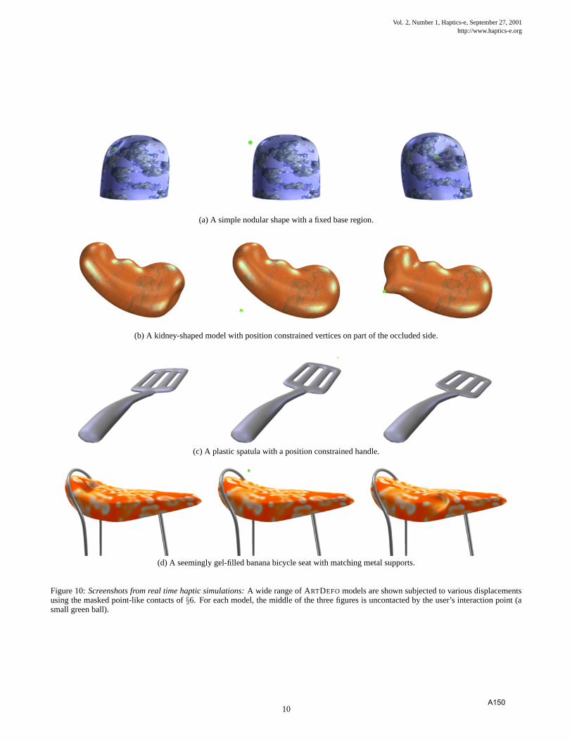
Vol. 2, Number 1, Haptics-e, September 27, 2001http://www.haptics-e.org
(a) A simple nodular shape with a fixed base region.
(b) A kidney-shaped model with position constrained vertices on part of the occluded side.
(c) A plastic spatula with a position constrained handle.
(d) A seemingly gel-filled banana bicycle seat with matching metal supports.
Figure 10: Screenshots from real time haptic simulations: A wide range of ARTDEFO models are shown subjected to various displacementsusing the masked point-like contacts of §6. For each model, the middle of the three figures is uncontacted by the user’s interaction point (asmall green ball).
10A150

Vol. 2, Number 1, Haptics-e, September 27, 2001http://www.haptics-e.org
Elastic Model # Vertices (n) # Faces Precomp (min) LUD % Simulate (ms)Nodule 130v (89 free) 256f 1.1 1.1% 0.05Kidney 322v (217 free) 640f 7.7 3.1% 0.13Spatula 620v (559 free) 1248f 45 5.7% 0.34Banana Seat 546v (245 free) 1088f 25 20.0% 0.15
Table 2: GF precomputation and simulation times for the BEM models depicted in Figure 10. All GFs corresponding to moveable freevertices (in Λ0
p) were computed, and the precomputation time (Precomp) of the largest model is less than an hour. As is typical of BEMcomputations for models of modest size (n < 1000), the O(n2) construction of the matrices (H and G in equation 8) is a significant portionof the computation, e.g., relative to the O(n3) cost of performing the LU decomposition (LUD %) of the A matrix. The last column indicatesthat submillisecond graphics-loop computations (Simulate) are required to determine the point contact deformation response of each model’sfree boundary.
# Updates, s LU Factor (ms) LU Solve (ms) (ΞE)(ETv) for n=100 (ms)10 0.54 0.03 0.3820 2.7 0.15 0.7440 19 0.58 1.7100 310 5.7 5.7
Table 3: Timings of CMA suboperations such as LU decomposition (LU Factor) and back-substitution (LU Solve) of the capacitance matrix,as well as the weighted summation of s GFs (per 100 nodes) are shown for different sizes of updated nodal constraints, s.
Figure 9: : Photograph of simulation in use: Users were able topush, slide and pull on the surface of the model using a point-likemanipulandum. Additionally, it was possible to change the surfacefriction coefficient, as well as the properties of the pressure mask,with noticeable consequences. The PHANToMTM (here model 1.0Premium) was used in all force feedback simulations, and is clearlyvisible in the foreground.
junction with capacitance matrix algorithms (CMAs). The data-driven CMA formulation highlights the special role of the capac-itance matrix in computer haptics as a contact compliance usefulfor generating contact force and stiffness models, and provides aframework for extending the capabilities of these models.
Additionally, the important special case of point-like contact wasaddressed with special attention given to the consistent definitionof contact forces for haptics. While this topic has been discussedbefore, we have introduced vertex masks to specify the distributionof contact forces in a way which leads to physically consistent forcefeedback models which avoid the numerical artifacts which lead tononsmooth rendering of contact forces on discrete models, as wellsas ill-defined contacts in the continuum limit.
There are several issues to be addressed by future work on thesimulation of LEMs for computer haptics.
One of the promises of linear GF models is that it should be pos-sible to precompute and haptically touch large-scale models even ifthey are too large to be graphically rendered. However, the CMApresented here is very efficient for small models (small n) and lim-ited constraints (small s), but further optimizations and required forprecomputing, storing and simulating large-scale LEMs. ExtendingLEMs to accomodate geometric and material nonlinearities is alsoan area of study. Results addressing these problems will appearshortly in subsequent publications.
A key challenge for interactively rendering elastic models is theplausible approximation of friction in the presence of multiple dis-tributed elastic-rigid and elastic-elastic contacts. While large con-tact areas are a potential problem for LEM haptics, i.e., due tolarge update costs, the accompanying collision detection and fric-tion problems appear to be at least as difficult. Incorporation ofLEMs into hybrid interactive dynamical simulations is also a rela-tively unexplored area.
Finally, the same issues (perceptible force regularity and spatialconsistency) which motivated our approach for a single point-likecontact, also arise for multiple point-like contacts and in generalwith multiple distributed contacts. The tight coupling of force stiff-nesses between all contact zones, and therefore each (networked)force feedback device, can make this a difficult problem in prac-tice.
A Justification of Interpolated TractionDistributions for Point Contact
This section derives the nodal boundary conditions associated witha localized point contact at an arbitrary mesh location. The prac-tical consequence is that the discrete traction distribution may beconveniently interpolated from suitable nearby nodal distributionsor masks.
Given a continuous surface traction distribution, p(x), a corre-sponding discrete distribution Φ(x)p may be determined by a suit-able projection into L of each Cartesian component of p(x). Forexample, consider the projection of a scalar function on Γ definedas the minimizer of the scalar functional E : R
3n7→ R,
E(p) =
∫
Γ
[
‖p(x) − Φ(x)p‖22 + ‖BΦ(x)p‖2
2
]
dΓx,
where B :L 7→R is some linear operator that can be used, e.g., to
11A151

Vol. 2, Number 1, Haptics-e, September 27, 2001http://www.haptics-e.org
penalize nonsmooth functions, and Φ(x) : R3n
7→ R3 is a nodal
interpolation matrix defined on the surface,
Φ(x) = [φ1(x)φ2(x) · · ·φn(x)] ⊗ I3, x ∈ Γ,
where I3 is the 3-by-3 identity matrix. The Euler-Lagrange equa-tions for this minimization are
∑n
j=1
(∫
Γ[φi(x)φj(x) + (Bφi(x)) (Bφj(x))] dΓx
)
pj
=∫
Γφi(x)p(x)dΓx i = 1, 2, . . . , n,
which, in an obvious notation, is written as the linear matrix prob-lem
Ap = f (36)
to be solved for the nodal traction values p. Note that A has unitsof area.
The relevant traction distribution for point-like contact is a scale-independent concentrated point load
p(x) = pδ(x) = f
δδ(x − xδ)
which models a force f δ delivered at xδ∈Γ. The force n-vector in
equation (36) has components
fi = φi(xδ)f δ
and the corresponding pressure distribution’s nodal values are
p = A−1
f.
For compactly supported basis functions, φi(x), f has only a smallnumber of nonzero components for any given x. Hence φi(x
δ) arethe interpolation weights describing the contribution of the nearbynodal pressure distributions, here specified by the columns of A−1.
As an example, consider the important case where L is a contin-uous piecewise linear function space with φi(xj) = δij . This wasthe space used in our implementation. In this case, at most onlythree components of f are nonzero, given by the indices i1, i2, i3which correspond to vertices of the contacted triangle τ δ , i.e., forwhich xδ
∈ τ δ . The values φi(xδ) are the barycentric coordinates
of xδ in τ δ . The pressure distribution’s nodal values are then
p = A−1
f (37)
=
3∑
k=1
(
A−1)
:ikfik
=
3∑
k=1
φik(xδ)
[
(
A−1)
:ikf
δ]
=3
∑
k=1
φik(xδ)p(ik), (38)
where p(ik) is the pressure distribution corresponding to the appli-cation of the load directly to vertex ik, and ():ik
refers to blockcolumn ik of the matrix. Therefore the piecewise linear pressuredistribution for a point load applied at a barycentric location on atriangle is equal to the barycentric average of the pressure distri-butions associated with the point load applied at each of the trian-gle’s vertices. This may be recognized as an elastic generalizationof force shading [27] for rigid models.
Note that the jth column of A−1 is a vertex mask that describesthe nodal distribution of the load applied to the jth vertex. Modify-ing the penalty operator B results in masks with varying degrees ofsmoothness and spatial localization.
References
[1] Oliver Astley and Vincent Hayward. Multirate haptic sim-ulation achieved by coupling finite element meshes throughnorton equivalents. In Proceedings of the IEEE InternationalConference on Robotics and Automation, 1998.
[2] Remis Balaniuk. Building a haptic interface based on a buffermodel. In Proceedings of the IEEE International Conferenceon Robotics and Automation, 2000.
[3] James R. Barber. Elasticity. Kluwer Press, Dordrecht, firstedition, 1992.
[4] C. A. Brebbia, J. C. F. Telles, and L. C. Wrobel. Boundary El-ement Techniques: Theory and Applications in Engineering.Springer-Verlag, New York, second edition, 1984.
[5] Morten Bro-Nielsen. Surgery simulation using fast finite ele-ments. Lecture Notes in Computer Science, 1131:529–, 1996.
[6] Morten Bro-Nielsen and Stephane Cotin. Real-time volu-metric deformable models for surgery simulation using fi-nite elements and condensation. Computer Graphics Forum,15(3):57–66, August 1996.
[7] Murak Cenk Cavusoglu and Frank Tendick. Multirate sim-ulation for high fidelity haptic interaction with deformableobjects in virtual environments. In Proceedings of the IEEEInternational Conference on Robotics and Automation, SanFrancisco, USA, 2000.
[8] S. Cotin, H. Delingette, and N. Ayache. Realtime elastic de-formations of soft tissues for surgery simulation. IEEE Trans-actions On Visualization and Computer Graphics, 5(1):62–73, 1999.
[9] Stephane Cotin, Herve Delingette, and Nicholas Ayache. Effi-cient linear elastic models of soft tissues for real-time surgerysimulation. Technical Report RR-3510, Inria, Institut Na-tional de Recherche en Informatique et en Automatique, 1998.
[10] Diego d’Aulignac, Remis Balaniuk, and Christian Laugier. Ahaptic interface for a virtual exam of a human thigh. In Pro-ceedings of the IEEE International Conference on Roboticsand Automation, San Francisco, USA, 2000.
[11] Gilles Debunne, Mathieu Desbrun, Alan Barr, and Marie-Paule Cani. Interactive multiresolution animation of de-formable models. In N. Magnenat-Thalmann and D. Thal-mann, editors, Computer Animation and Simulation ’99,SpringerComputerScience, pages 133–144. Springer-VerlagWien New York, 1999. Proceedings of the EurographicsWorkshop in Milano, Italy, September 7–8, 1999.
[12] Y. Ezawa and N. Okamoto. High-speed boundary elementcontact stress analysis using a super computer. In Proc. of the4th International Conference on Boundary Element Technol-ogy, pages 405–416, 1989.
[13] Sarah Gibson, Christina Fyock, Eric Grimson, Takeo Kanade,Rob Kikinis, Hugh Lauer, Neil McKenzie, Andrew Mor, ShinNakajima, Hide Ohkami, Randy Osborne, Joseph Samosky,and Akira Sawada. Volumetric object modeling for surgicalsimulation. Medical Image Analysis, 2(2):121–132, 1998.
[14] Sarah F. Gibson and Brian Mirtich. A survey of deformablemodels in computer graphics. Technical Report TR-97-19,Mitsubishi Electric Research Laboratories, Cambridge, MA,November 1997.
12A152

Vol. 2, Number 1, Haptics-e, September 27, 2001http://www.haptics-e.org
[15] Gene H. Golub and Charles F. Van Loan. Matrix Computa-tions. Johns Hopkins University Press, Baltimore and Lon-don, third edition, 1996.
[16] William W. Hager. Updating the inverse of a matrix. SIAMReview, 31(2):221–239, June 1989.
[17] K. V. Hansen and O. V. Larsen. Using region-of-interest basedfinite element modeling for brain-surgery simulation. LectureNotes in Computer Science, 1496:305–, 1998.
[18] Friedel Hartmann. The mathematical foundation of structuralmechanics. Springer-Verlag, New York, 1985.
[19] C.-H. Ho, C. Basdogan, and M. A. Srinivasan. Efficient point-based rendering techniques for haptic display of virtual ob-jects. Presence, 8(5):477–491, 1999.
[20] Doug L. James. http://www.cs.ubc.ca/˜djames/deformable.
[21] Doug L. James and Dinesh K. Pai. ARTDEFO: Accurate RealTime Deformable Objects. Computer Graphics, 33(AnnualConference Series):65–72, 1999.
[22] A. M. Abu Kassim and B. H. V. Topping. Static reanalysis:a review. Journal of Structural Engineering, 113:1029–1045,1987.
[23] U. Kuhnapfel, H.K. Cakmak, and H. Maaß. 3d modeling forendoscopic surgery. In Proceedings of IEEE Symposium onSimulation, pages 22–32, Delft University, Delft, NL, October1999.
[24] Charles Loop. Smooth subdivision surfaces based on tri-angles. Master’s thesis, University of Utah, Department ofMathematics, 1987.
[25] K. W. Man, M. H. Aliabadi, and D. P. Rooke. Analysis ofContact Friction using the Boundary Element Method. InM. H. Aliabadi and C. A. Brebbia, editors, ComputationalMethods in Contact Mechanics, chapter 1, pages 1–60. Com-putational Mechanics Publications and Elsevier Applied Sci-ence, 1993.
[26] T. H. Massie and J. K. Salisbury. The phantom haptic inter-face: A device for probing virtual objects. In ASME WinterAnnual Meeting, Symposium on Haptic Interfaces for VirtualEnvironment and Teleoperator Systems, Chicago, IL, Nov.1994.
[27] Hugh B. Morgenbesser and Mandayam A. Srinivasan. Forceshading for haptic shape perception. In Proceedings of theASME Dynamics Systems and Control Division, volume 58,1996.
[28] Dinesh K. Pai, Kees van den Doel, Doug L. James, JochenLang, John E. Lloyd, Joshua L. Richmond, and Som H. Yau.Scanning Physical Interaction Behavior of 3D Objects. InComputer Graphics Proceedings (SIGGRAPH 2001). ACMSiggraph, 2001.
[29] G. Picinbono, J. C. Lombardo, H. Delingette, and N. Ayache.Anisotropic elasticity and force extrapolation to improve re-alism of surgery simulation. In Proceedings of IEEE Inter-national Conference on Robotics and Automation, San Fran-cisco, USA, 2000.
[30] William H. Press, Brian P. Flannery, Saul A. Teukolsky, andWilliam T. Vetterling. Numerical Recipes: The Art of Scien-tific Computing, chapter Sherman-Morrison and Woodbury,pages 66–70. Cambridge University Press, Cambridge, 1987.
[31] R. Ramanathan and D. Metaxas. Dynamic deformable mod-els for enhanced haptic rendering in virtual environments. InIEEE Virtual Reality Conference, 2000.
[32] P. Schroder, D. Zorin, T. DeRose, D. R. Forsey, L. Kobbelt,M. Lounsbery, and J. Peters. Subdivision for modeling andanimation. SIGGRAPH 99 Course Notes, August 1999.
[33] Sensable Technologies, Inc. GHOST SDK,http://www.sensable.com.
[34] Yan Zhuang and John Canny. Haptic interaction with globaldeformations. In Proceedings of the IEEE International Con-ference on Robotics and Automation, 2000.
[35] O. C. Zienkiewicz. The Finite Element Method. McGraw-Hill Book Company (UK) Limited, Maidenhead, Berkshire,England, 1977.
[36] C. B. Zilles and J. K. Salisbury. A constraint-based god-objectmethod for haptic display. In ASME Haptic Interfaces for Vir-tual Environment and Teleoperator Systems, volume 1, pages149–150, Chicago, IL (US), 1994.
13A153

Scanning Physical Interaction Behavior of 3D Objects
Dinesh K. Pai, Kees van den Doel, Doug L. James, Jochen Lang, John E. Lloyd, Joshua L. Richmond, Som H. Yau
Department of Computer Science, University of British Columbia, Vancouver, Canadapai,kvdoel,djames,jlang,lloyd,jlrichmo,[email protected]
(a) Real toy tiger. By de-sign, it is soft to touchand exhibits significantdeformation behavior.
(b) Deformable model oftiger scanned by our sys-tem, with haptic interac-tion.
(c) Real clay pot, withglazed regions. The potexhibits a variety of con-tact textures and sounds.
(d) Virtual interactionwith scanned model ofpot; includes contact tex-ture and contact sounds.
Figure 1: Examples of behavior models scanned by our system
Abstract
We describe a system for constructing computer models ofseveral aspects of physical interaction behavior, by scanningthe response of real objects. The behaviors we can suc-cessfully scan and model include deformation response, con-tact textures for interaction with force-feedback, and contactsounds. The system we describe uses a highly automatedrobotic facility that can scan behavior models of whole ob-jects. We provide a comprehensive view of the modelingprocess, including selection of model structure, measure-ment, estimation, and rendering at interactive rates. Theresults are demonstrated with two examples: a soft stuffedtoy which has significant deformation behavior, and a hardclay pot which has significant contact textures and sounds.The results described here make it possible to quickly con-struct physical interaction models of objects for applicationsin games, animation, and e-commerce.
Keywords: Behavioral Animation, Deformations, Haptics, Multi-
media, Physically Based Modeling, Robotics, Sound Visualization
1 Introduction
Real 3D objects exhibit rich interaction behaviors which in-clude how an object deforms on contact, how its surface feels
when touched, and what kinds of sounds it makes when oneinteracts with it. These aspects of visual, haptic1, and au-ditory behavior provide important interaction cues and in-crease the sense of presence in virtual environments suchas games. Despite recent progress in deformation modeling(e.g., [37, 7, 18]), haptic rendering (e.g., [32]), and auditorydisplays (e.g., [12]), these aspects are either entirely missingfrom models used for computer graphics and interaction, ormust be painstakingly added by highly skilled professionals.We believe that a major reason for this unfortunate situationis the difficulty of constructing these complex multimodalmodels by hand. In this paper we show how this problemcan be solved by scanning the behavior of real objects.
Constructing behavior models requires not only acquiringmeasurements of real object behavior, but also designingmathematical models whose parameters can be effectivelyestimated from the measurements, and can be effectivelyused for realistic rendering. Each of these steps is importantfor successfully modeling real object behavior. We give de-tailed descriptions of how this can be done for three aspectsof interaction behavior: (1) deformation models which canbe rendered both visually and haptically; (2) contact texturemodels for capturing surface friction and roughness for hap-tic display and dynamics simulation; and (3) contact soundmodels for synthesizing interaction sounds, including soundsof continuous interaction.
Figure 1 shows some behavior models acquired by oursystem. Of course, it is somewhat difficult to show real timebehavior on paper. The accompanying video demonstratesthe behavior models better.
In this paper we also describe how the acquisition of thesemodels can be automated using a highly integrated roboticmeasurement facility, and how behavior models can be reg-istered relative to a geometric model of an object. Eventhough our facility is an expensive prototype and uses sophis-ticated robotics for interaction and behavior measurement,we believe it can be practical and economical for modeling
1haptics refers to the sense of touch.
Permission to make digital or hard copies of all or part of this work forpersonal or classroom use is granted without fee provided that copiesare not made or distributed for profit or commercial advantage and thatcopies bear this notice and the full citation on the first page. To copyotherwise, to republish, to post on servers or to redistribute to lists,requires prior specific permission and/or a fee.
ACM SIGGRAPH 2001, 12-17 August 2001, Los Angeles, CA, USA© 2001 ACM 1-58113-374-X/01/08...$5.00
87A154

because the facility can be shared by multiple users. Thetechniques we describe can be used to construct a modelfoundry, similar to a VLSI chip foundry but in reverse. Userscould send real objects to such a foundry and receive in re-turn a behavior model of the object.
It is helpful to compare the work presented here to 3Dgeometric modeling, from which we draw inspiration and in-struction. 3D geometric models can be constructed by handusing 3D modeling software and for some special applica-tions, this hand modeling and editing is essential. However,3D scanning technology has dramatically changed the waysuch models are constructed. 3D geometry scanning makesit possible to capture fine details for unprecedented realism,but more importantly, empowers users with modest artistictalents with the ability to construct 3D models quickly andinexpensively. In a similar way, we expect that hand con-struction of interaction behavior will continue to be useful forsome applications (e.g., those requiring fine creative controlto match the context and narrative). But for many appli-cations in games, animation, and e-commerce, the ability toconstruct highly detailed behavior quickly and inexpensivelyusing the techniques we describe here could transform theway we construct models for 3D object interaction.
1.1 Related Work
We are not aware of any other system capable of scanningmodels of contact interaction behavior such as that describedin this paper. However, each component of our system hasmany connections to previous work that we discuss in therelevant sections below. Here we briefly discuss related workin the general area of building models of 3D objects by mea-suring the real world.
Almost all the work in the area of modeling real world ob-jects in computer graphics has focused on geometric model-ing and reflectance modeling. In recent years there has beendramatic progress in scanning geometric models of 3D ob-jects (e.g., [17, 8, 33, 22, 23]). In part because of the highaccuracy of laser scanning, most of these techniques assumethat the range data are given and focus on estimating goodmeshes from the data. Techniques have also been developedfor geometry reconstruction from a few photographs [11] oreven from a simple desktop system with a wand [2]. Acquir-ing the reflectance properties of existing objects has alsobeen an active research area (e.g., [33, 9, 31, 15]). Our workhas parallel goals with this type of automated model ac-quisition, but differs in terms of types of models acquired.Acquiring interaction models is more difficult because of thenecessity of actually interacting and making contact withthe objects to be measured.
Our work has some connections with image based tech-niques [4] and motion capture in that a recording can beconsidered a simple model of behavior, which can be editedand transformed (e.g., [26]). With few exceptions they havegenerally not been used for estimating parameters of physicalmodels. They also do not account for inputs to the motion,and therefore can not be directly used for simulating theeffects of new inputs.
Measuring the real world requires a certain amount of in-frastructure and several groups have developed measurementfacilities for this purpose. We mention the Cornell LightMeasurement facility [15], the Columbia/Utrecht facilityused for constructing a reflectance and texture database [9],the CMU Virtualized RealityTM laboratory [41], the Berke-ley Light Stage [10]. Field-deployable systems includethe Digital Michelangelo project [23] and the IBM Pieta
project [31].Our own facility is perhaps the most highly automated
and flexible system available today. It was designed to pro-vide one-stop shopping for a large number of measurementsrather than for highly accurate measurement. It requiredsignificant developments in robotics to control and coordi-nate the various measurement and actuation subsystems ofthe facility. We have previously described the robotics as-pects of teleprogramming and motion planning for the sys-tem, and measurement techniques for sound and deforma-tion (e.g., [25, 24]). However, the present paper is the firstto describe the complete process of modeling interaction be-haviors, from real object to rendered model.
2 A Framework for Modeling Behavior
To help understand how to construct useful models of realobjects, it is helpful to break the task down into four steps:selection of model structure, measurement, parameter esti-mation, and rendering. In the following sections we detailhow these steps are carried out for acquiring models of de-formation, contact texture, and sound.
Selection of model structure
This defines the fundamental class of mathematical modelsthat will be used to represent real physical behavior. Inthis step we fix the structure and not the parameters of themodel.
We emphasize that this step is a creative act of modeldesign, in which the modeler balances the competing needsof the accuracy of the model’s predictions, rendering speed,ease of acquiring measurements, stability of parameter esti-mation, etc. It is tempting to think that the model is dic-tated by Physics and can be “looked up” in a textbook, butthis is far from the truth. In designing the model structureit is essential to realize that all models have a finite domainof applicability.
Measurement
In this step we acquire the data from the real world to con-struct the model. This step is critical since all subsequentresults depend on it. It is non-trivial for several reasons.First, we are interested in contact behavior which can notbe simply observed but must be “excited” by physically in-teracting with the object. Thus we not only need to measure,say, the sound produced by an object, but we also need away to hit the object in a carefully controlled manner to pro-duce the sound. Second,traditional measurement techniquesare designed for measuring material properties of small sam-ples of objects, but we would like to build models of entireobjects without destroying them or changing their essentialglobal properties. Thus it is necessary to be able to moveeither the object or the measuring instruments or both, toaccess different parts of the object. Third, we need to reg-ister the different measurements relative to each other. Wedo this by registering all measurements relative to a geomet-ric model of the object. For instance, this allows us to usethe surface roughness of a particular point on the surfaceto drive the sound produced by scraping the surface at thatpoint. However this means that we must first acquire a ge-ometric model of the object prior to scanning the behavior.Finally, to interpret the raw data the instruments need tobe calibrated. We do this using special calibration objects,
88A155

but auto-calibration techniques could also be used. To facil-itate this kind of measurement we have built an integratedrobotic measurement facility described in §3.
Parameter estimation
Estimation connects measurements to models. It is im-portant to realize that estimation problems are frequentlyill-posed and can lead to very sensitive inverse problems.Therefore it is necessary to pre-process the raw data, useregularization (which can be done in a natural way usingBayesian priors), and to use robust estimation techniques.As an example, direct fitting of sound models to sound wave-forms by least-squares techniques produces very poor resultsin the presence of noise. We describe robust techniques forestimation which we found work well for the various estima-tion problems described below.
Rendering
Finally, the estimated models must be rendered, to pro-duce deformations, haptic forces, and sounds. This step, ofcourse, is the primary motivation for the previous steps andinfluences design decisions throughout. In particular, sincewe are interested in interaction behavior, it is important thatthe models are rendered at interactive rates. We describeimplemented algorithms suitable for interactive rendering ofdeformation, forces, and sounds. The rendering step is alsoimportant for validation of the scanned model, i.e., deter-mining whether the estimated model approximates realitysufficiently well for a given purpose. For computer graphicsand interaction, it is difficult to design sensible quantitativemetrics of model validity, and one must largely rely on userperception. We show results comparing the behavior of realobjects to simulations of the scanned behavior models.
3 Measurement System for Interaction Be-havior
Carefully acquiring the measurements required for modelbuilding is often the most challenging part of the modelingprocess. For acquiring the kind of contact measurements weneed, we have developed the UBC Active Measurement facil-ity (ACME), a highly automated robotic measurement facil-ity. The robotics aspects of the facility have been previouslydescribed in detail [25]. For completeness, we briefly outlineit here. We note, however, that the techniques described be-low do not depend on the use of this particular facility whichwas designed to provide a large variety of measurements; asimpler measurement set up could be constructed to buildspecific kinds of models. As with 3D geometry scanning, weexpect that in the future it may be possible to build portableor desktop versions of such a measurement system.
Fig. 2 shows the facility which consists of a variety of sen-sors and actuators, all under computer control. Its majorsubsystems include: a 3 DOF Test Station (bottom of im-age) used for precise planar positioning of the test object;a Field Measurement System (shown at the top left) con-sisting of a Triclops trinocular stereo vision system, a highresolution RGB camera, and a microphone, all mounted ona 5 DOF positioning robot; and a Contact MeasurementSystem (CMS, shown on the right) consisting of a Puma260 robot equipped with a force/torque sensor, mounted ona linear stage. The CMS is the key subsystem for contactmeasurements as it is used to interact with the object to
Figure 2: ACME Facility Overview
be modeled. The entire facility can be controlled from anylocation on the Internet. We will describe the use of the sen-sors and actuators for measurement in the relevant sectionsbelow.
4 Geometric Modeling
The geometric models required for registering other mea-surements can be produced by any geometry scanning andmesh generation method (e.g., [17, 8, 33, 28, 23]). Whilethe focus of this paper is not on geometric modeling, forcompleteness we will briefly outline our approach to geo-metric model construction starting from stereo range mea-surements.
Stereo range measurement
The main shape sensor in our measurement facility is atrinocular stereo vision system2 which is capable of produc-ing large amounts of viewpoint-registered range images atmodest resolutions (approx. 2-3 mm for a typical viewpoint),in close to real time. Accurate ranging relies on image fea-tures for matching between the stereo cameras; additionalfeatures can be attached or projected onto the surface.
Stereo range data is notoriously noisy, and for best re-sults it is filtered in several ways. First, range is calculatedwith variable mask sizes in a voting scheme. We also utilizethe checks and filters of the Triclops stereo library. Furtherprocessing of the data by volumetric reconstruction requiresapproximate surface normals at range data points. The nor-mals are estimated by plane fitting in local image neigh-borhoods. Further filtering of the range-data is performedbased on the quality of fit, the number of valid range-dataper neighborhood and the viewing angle of the plane.
Multresolution mesh construction
An initial triangle mesh is generated from the filtered rangedata using a volumetric approach by reconstruction softwareprovided courtesy of NRC of Canada [28]. The number andquality of triangles depends on the surface sampling density.Further processing is required to arrive at a useful geometricmodel since this mesh may not be watertight; it may includesome of the supporting Test Station surface; and there may
2A Color Triclops from Point Grey Research.
89A156

Figure 3: Clay Pot Mesh Reconstruction: (left) raw scanmesh (13150 vertices, 26290 faces) with various externalstray polygons; (middle) watertight base level (level 0) mesh(127 vertices, 250 faces) generated via simplification of theraw scan mesh; (right) level 3 subdivision connectivity mesh(8002 vertices, 16000 faces) generated using displaced sub-division surface style piercing of the raw scan mesh.
be erroneous surfaces due to noisy data. An example isshown in the left image of Figure 3.
Finally, we construct watertight subdivision connectivitytriangle meshes at several resolutions l = 0, 1, 2, . . . , L be-cause they are desirable for later modeling. Here we exploit acommon property of raw meshes produced from range data:while the region exterior to the object geometry may con-tain undesirable mesh features, the interior of the mesh is afair representation of the scanned surface. This allows theconstruction of multiresolution meshes by expanding and re-fining a surface inside the object using a normal piercingprocess similar to the construction of displaced subdivisionsurfaces [21] and normal meshes [16]. The coarse resolu-tion mesh is generated by simplifying the raw mesh (usingQSlim [13]) and possibly some minor editing to ensure thatthe mesh is free of defects such as in regions with poor rangedata. To ensure that the mesh expansion process is bounded,the raw mesh is manually closed if the NRC package pro-duces a large hole on the unimaged underside of the object;this was addressed for the tiger mesh by simply inserting alarge horizontal triangle.
While this approach to mesh construction is not robust,it produces meshes of sufficient quality that we were able toproceed with our main physical modeling objectives.
Texture mapping
Texture mapping is accomplished using calibrated color im-ages from the stereo vision system. The vertices of themeshes are projected into the color images using the pinholecamera calibration matrix, and triangles are tagged as visi-ble if their vertices and centroid are all visible. We select theimaged triangular area as the texture map if the product ofthe image area times the cosine between view direction andtriangle normal is maximum in all our images. We also ad-just the relative global brightness of all color texture images.The texture maps could be readily improved by blending ofthe local textures over the entire map eliminating abruptbrightness changes at edges, as in [27].
5 Deformation Modeling
Selection of model structure
We use linear elastostatic models for deformable objectssince these models can be simulated at interactive rates [18],and linearity makes parameter estimation easier. Most im-
portant, linear elastic models can be characterized usingGreen’s functions, which capture the input-output behav-ior of the object’s boundary for a given set of boundaryconditions; therefore there is no need to observe or estimatequantities in the interior of the object.
It is a practical consideration that the model must be fix-tured for it to be deformed by ACME’s robots. Therefore westart by assuming that the physical object will be measured(and rendered) while attached to a support, like the TestStation. The linear elastostatic model then approximatesthe displacement response u = u(l) of the resolution l meshvertices due to applied surface tractions3 p=p(l) by
u = Up or u(l) = U(l)p(l). (1)
Here u and p are block vectors of length n with 3-vector ele-ments, where the displacement and traction at the kth vertexis uk and pk, respectively; U is a square n(l)-by-n(l) block ma-trix with 3-by-3 matrix elements. The kth block column U:k
describes the displacement response contribution from thekth applied traction pk. The diagonal blocks Ukk describethe self-compliance of the kth vertex, and play an importantrole in defining vertex stiffnesses for force-feedback render-ing [19]. The traction vector at a vertex is the force overthe area of the one-ring of a vertex. The force is distributedlinearly over the area as a hat function located at the vertex.
The key behavior of the model is characterized by thedisplacement response of the unfixtured free surface due toforces applied to the free surface. This corresponds to theonly interesting measurable portion of the U matrix, whichin turn is related to the discrete Green’s function matrix [19]for the free boundary. For instance, rows of U correspondingto vertices attached to the fixtured support necessarily havezero displacement values; these same vertices correspond tocolumns which are not exposed and therefore can not beactively inspected.
Finally, once the Green’s function matrix for a fixture con-figuration is known, deformations of the object can be sim-ulated efficiently using fast matrix updating techniques [19].
Measurement
Objects to be measured, such as the stuffed toy tiger shownin Figure 1, are fixed to the Test Station. Deformation mea-surements record surface displacements and contact forcesresulting from active probing with ACME’s CMS robot arm.During deformation the position of the contact probe can becontinuously monitored at 100 Hz. The robot arm’s wristforce sensor is capable of recording the six-dimensional force-torque wrench at the tip of the probe at 1000 Hz.
The robot probes surface locations corresponding to ver-tices of the geometric model at the desired reconstructionresolution4 l. The position of the contact probe measuresthe displacement of the contacted vertex uk, while the force-torque sensor measures the contact force. The effective con-tact traction pk is the force divided by the effective vertexarea (one third of the sum of adjacent triangle areas). Sincethere are no other applied tractions on the free or fixed sur-faces, the complete traction vector p is zero except for thesingle contact traction pk. In the following we describe howthe deformation of the free surface is measured and mappedonto the vertices in order to estimate u.
3Traction is the force per unit area, similar to pressure.4To avoid measurement artifacts the scale of the mesh is larger
than the measurement probe’s contact area.
90A157

Figure 4: 2D Flow on tiger, poked near the neck.
The surface deformation of the object is measured visu-ally using the Triclops trinocular stereo-vision system in theField Measurement System (FMS) of ACME. The measure-ment is based on tracking visual surface features in threespatial dimensions in a range-flow [42] approach. Severalmethods for calculating dense range-flow from stereo andoptical flow exist [41, 43, 34].
Our method utilizes redundancy in the imagery from thetrinocular stereo-system to increase robustness [20]; It issummarized as:
• Segment image into “object surface” and “other,” basedon the geometric model of the undeformed object.
• Calculate range from stereo.
• Calculate simultaneous optical flow in images from eachcamera for the “object surface”.
• Combine optical flow by voting and map the result intothree dimensions based on range data.
• Use the “range-flowed” object surface to segment thenext image in the sequence and continue with stereocalculations as above.
The optical flow during deformation measurement is shownin Figure 4. In our approach, the surfaces need sufficientvisual texture because of the reliance on stereo vision andoptical flow. Most objects have sufficient visual texture forstereo matching but if not non-permanent visual texture maybe applied (e.g., using pins, stickers, or water soluble paint).
The next step in surface deformation measurement is themapping of range flow vectors to displacements of verticesof a chosen mesh level. Flow vectors are associated with astart position on a triangular patch of the undeformed mesh.We estimate the displacement of a vertex with a robust av-eraging process rather than just using the closest flow vectorto a vertex (see, for example, [1] for a discussion on robustmotion estimation). The flow vectors associated with trian-gular patches joined at a vertex are median filtered. Thisis followed by a weighted average based on distance fromthe vertex. The flow vectors have to be dense enough onthe surface relative to the mesh level for this process to berobust. In our set-up, we get high density by positioning
the camera close to the object (≈ 0.8m). The measured dis-placement u covers surface area visible from a chosen viewpoint. In the estimation section below, we discuss how tocombine multiple measurements for the same contact vertex.
Parameter estimation
Our approach to the estimation of the matrix U from themeasurements of displacement u and traction p addressestwo main issues: (1) noise in the form of outliers in the dis-placement measurement and (2) incomplete measurements.Outliers can, on occasion, still be observed in the displace-ment measurement despite the above described filtering pro-cess. These outliers originate from consistent incorrect flowvectors due to mismatches in the range-flow or in the stereoprocessing over an image area. Incomplete measurementsarise from partially observed object surfaces, from reacha-bility limits of the CMS and from anisotropic responses ofthe object to probing.
A single block element Uij describes the relationship be-tween the displacement ui and a single applied traction pj :
ui = Uijpj .
For each element, we obtain m≤M measurements by prob-ing each vertex location M times. We arrive at a standardleast squares problem to be solved for UT
ij :
[p1
jp2j · · · pm
j
]TUT
ij =[u1
i u2i · · · um
i
]T
We solve this least squares problem if our measured trac-tions are a response to a set of probe directions which span3-space. This guarantees that we excite the model in all di-rections. However, because of the possibility of (in general)noncompliant responses combined with the limited resolu-tion of the measurements, this does not guarantee that thesolution (Uij)
T has full rank. Therefore, we calculate thesolution by means of the truncated singular value decom-position (TSVD). We truncate the singular values at theapproximate resolution of the traction measurements. Fur-thermore, we select a subset of measurements if we observean unsatisfactory fit of the estimated (Uij)
T and repeat.This subset selection process is performed using the leasttrimmed squares (LTS) method [29], implemented efficientlyas in [30]. This process is robust even if (M −4)/2 measure-ments are spoiled.
Figure 5: Plots of estimated displacement responses: (left)Missing observations result in unestimated response compo-nents (shown in black); the remaining nodes are color codedwith red indicating the greatest displacement and blue theleast. (right) These values are estimated by an interpolatingreconstruction to obtain the final deformation responses.
At this stage of the estimation process, the measureddisplacement field columns of U still contain unestimated
91A158

elements due to missing observations of the deformed sur-face (shown in Figure 5). This problem can be minimizedby obtaining more measurements but not entirely avoided.Scattered data reconstruction is used to fill in elements foreach column individually. We currently interpolate missingdisplacements by solving Laplace’s equation over the set ofunestimated vertices, but better methods are currently be-ing investigated. The result of this interpolation process isshown in Figure 5.
Finally, in order to improve rendering quality and reducemeasurement and estimation time we exploit the multires-olution mesh structure to optionally infer Green’s functionresponses for unmeasured vertices. This is done by activelypoking the model at a resolution (l − 1) one level coarserthan the resolution l used to estimate displacement fields(illustrated in Figure 6). The kth odd vertex on level l hasa response U:k inferred if both even vertices (k1, k2) of itsparent edge have responses. If so, the kth response U:k is lin-early interpolated from the two parent responses, (U:k1 , U:k2).The local responses, Ukk and Ujk when vertex j is a one-ringneighbor of k, are handled differently.
Unlike long range displacement influences which aresmoothly varying, these local values are associated with acusp in the displacement field. Simple interpolation for thesevalues is biased and leads to incorrect contact forces duringrendering. Instead, the local values are computed as theweighted average of parent responses which have had theirlocal parameterizations smoothly translated from even ver-tex k∗ to odd vertex k, e.g., Ukk is linearly interpolated from(Uk1k1 ,Uk2k2) not (Ukk1 ,Ukk2). This shifting of the parent’slocal response before averaging yields a good estimator ofthe local response at vertex k. The resulting displacementfield U:k is also linearly independent of U:k1 and U:k2 .
Figure 6: Multiresolution Mesh and Contact Sampling Pat-tern: (left) Coarse l = 0 parameterization of model, used foractive contact measurement, displayed on finest l = 2 dis-placed subdivision surface mesh; (right) yellow points drawnon the l = 1 resolution mark the nodes at which the system’sdisplacement response to applied tractions was either mea-sured (even vertices) or inferred (odd vertices).
Rendering
By design, the Green’s function models can be rendered atinteractive rates using the algorithm described in [18, 19].Contact forces are rendered using a PHANToM force-feedback interface with contact force responses computedusing vertex pressure masks [19]. The multiresolution de-forming surface is also displacement mapped using displacedsubdivision surfaces [21] to add extra geometric detail to themodel. Figure 1 and the accompanying video (and the CALdemonstration) show interaction with scanned tiger modelusing the PHANToM. In general the results are quite sat-
isfactory, capturing non-local effects such as the movementof the head when the back of the tiger is poked. The modeldoes show some of the limitations of the linear model struc-ture for large input displacements, with somewhat exagger-ated deformations. For moderate input displacements5, thescanned model behaves quite realistically.
6 Contact Texture
Selection of model structure
Contact texture denotes the way an object feels when it isrubbed or scraped. The two principal aspects we focus onin this paper are friction and surface roughness.
For modeling friction, we use the standard “textbook”Coulomb friction model
f f = −µ ‖fn‖um (2)
where ff is the frictional force, µ is the coefficient of fric-tion (and the model parameter to be determined), fn is thenormal force, and um is a unit vector in the direction ofmotion.
Surface roughness is a more elusive property and wholebooks have been written on how to model it [38]. Rough-ness is usually associated with small-scale variations in thesurface geometry, which create variations in the tangentialcontact force proportional to the normal force. These tan-gential force variations can be modeled as local variations µin the coefficient of friction. Combined with µ, this yieldsan effective coefficient of friction µe for a given displacementx along some particular surface direction:
µe(x) = µ + µ(x).
This formulation has the advantage of unifying haptic ren-dering of friction and roughness, particulary with commer-cial haptic devices like the PHANToM which implementtheir own contact and friction algorithms which may notcorrespond to the textbook model of Coulomb friction.
Forces due to roughness tend to have some randomnessbut often also contain periodic components, particularly inhuman artifacts. We assume that the roughness is isotropicand that people are sensitive only to statistical features ofthe roughness force variation, and can not discern the spe-cific waveform. To capture both randomness and periodicitywe model the friction variations µ(x) as an autoregressiveAR(p) process, driven by noise, so that
µ(x) = µ(k∆) ≡ µ(k) =
p∑
i=1
aiµ(k − i) + σε(k)
where k is the sample index, ∆ is the spatial discretization,σ is the standard deviation of the input noise, and ε(k) is azero-mean noise input with standard deviation of one. Themodel parameters to be determined are the ai and σ.
The AR model is very suitable for real-time simulationand rendering, and typically one needs only a few parametersto reflect the roughness properties (as illustrated by Fig. 7).An AR(2) model is often sufficient in practice because itallows the modeling of a random sequence combined withone principal frequency.
5approximately < 15% of the tiger’s diameter
92A159

0 2 4 6 8 100
0.05
0.1
0.15
0.2
0.25
0 2 4 6 8 100
0.05
0.1
0.15
0.2
0.25
Figure 7: (left) Measured values of µe for a 10 mm displacementalong a rough section of the clay pot shown in Fig. 8. (right)Simulation of µe with µ = 0.142 and µ reproduced by an AR(2)model with a1 = .783, a2 = .116, and σ = 0.0148.
Measurement and Estimation
Friction and surface roughness are noticeable in terms ofthe forces they produce on a contacting instrument. Hencewe can measure them in the same way: the robotic systemperforms a series of local rubs over the object surface witha probe (attached to a 6 DOF force sensor; Fig. 8) and theresulting force profiles are then analyzed.
The object’s surface mesh representation is used to plan“where and how” to do the rubbing. At present, the systemassigns a contact texture model to each mesh vertex. This isdetermined either by explicit measurement, or by the inter-polation of models at nearby vertices. The system employsa process of “active exploration”, in which models are ini-tially sampled over the object surface at a low resolution,with further, higher resolution sampling in areas where themodel parameters change significantly.
Figure 8: (left) Robotic system rubbing the pot to determinecontact texture. (right) Surface friction map for the claypot, in which the brightness is scaled according to the localvalue of µ on the surface (with white corresponding to themaximum value of µ = 0.5). The enameled portions of thepot, with µ ≈ 0.09, are clearly visible. The ornament on topof the pot was not sampled.
The nominal friction coefficient µ is estimated first. If thesurface normal n were known accurately, one could directlydetermine fn and ff in Eq.(2) and use this to solve for µ.However, n is known only approximately (due to uncertaintyin the surface mesh and the actual contact location), andalso varies along the path. To compensate for this, we strokethe surface twice: once in a forward direction and once ina reverse direction. At any point along the path, we thenhave a force value f+ which was measured during the forwardmotion, and another value f− which was measured duringthe reverse motion.
f+ and f− each have components parallel to the surface
normal n, along with friction components f+f and f−f which
lie opposite to the motion directions and are perpendicularto n. Now even if n is unknown, and the magnitudes off+ and f− differ, µ can still be estimated from the angle θbetween f+ and f−:
µ = tan(θ/2).
This calculation is quite robust, as it is independent of travelspeed, the probe contact force and orientation, and of coursethe surface normal itself. By averaging the values of µ ob-tained at various points along the path, a reasonable esti-mate for µ over the whole path may be obtained. Our abilityto determine µ reliably is illustrated in Fig. 8.
The values of n at each path point can also be estimatedfrom the direction of (f+
f +f−f ) and used to produce a smooth
(typically quadratic) model of n(x) along the path.To calculate the effective friction, we use n(x) to relate µe
to the observed force values f acting on the probe tip:
f = fn[n(x)− µeum(x)],
where um(x) is the direction of motion along the path and fn
is the magnitude of the normal force. The unknowns in thisequation are fn and µe. Solving for µe at every path point xyields µe(x). An AR model is then fitted to µ(x) = µe(x)−µ,using autoregressive parameter estimation via the covariancemethod (e.g., the arcov function in MATLAB).
Rendering
To demonstrate the rendering of contact texture, we useda PHANToM haptic device to implement a virtual environ-ment in which a user can rub an object with a point contact(represented as a red ball in the video). The GHOST soft-ware supplied with the PHANToM was used to perform col-lision detection and to generate the corresponding contactand frictional forces.
The friction value at the point of contact is generated byweighting the AR parameters at each vertex by the barycen-tric coodinates in the triangle. The distance traveled alongthe surface divided by the spatial discretization ∆ of themeasurements determines the number of values to generateusing the AR model. The last 2 values generated are theninterpolated to obtain the effective coefficient of friction µe.This value is passed to both the static and dynamic frictionparameters in GHOST.
The resulting contact textures are quite convincing; it iseasy to distinguish between the different surface prepara-tions of the clay pot using the haptics alone. These resultsare best evaluated using the PHANToM haptic device (e.g.,in our CAL demo) though Figs. 7 and 8 give a good indica-tion of the sensitivity of our measurement technique.
7 Sound Modeling
Selection of model structure
We model the contact sounds of an object by filtering an ex-citation (the “audio-force”) through a modal resonator bankwhich models the sonic response of the object. The detailsof this technique are explained in [39]. For this we need toacquire both a modal resonance model of the object, whichwill depend on its shape and internal composition, and anexcitation model, which will depend mainly on the surfacestructure.
93A160

The modal model M = f ,d,A, consists of a vector fof length N whose components are the modal frequenciesin Hertz, a vector d of length N whose components are the(angular) decay rates in Hertz, and an N × K matrix A,whose elements ank are the gains for each mode at differentlocations. The modeled response for an impulse at locationk is given by
yk(t) =
N∑
n=1
anke−dnt sin(2πfnt), (3)
for t ≥ 0 (and is zero for t < 0).The surface texture generating the audio-force can be
modeled in real-time by filtering an appropriate noise sourcewith the location dependent autoregressive filter models ob-tained from the surface measurements described in Section 6.
For audio we need to know the audio surface texture ata much higher resolution than for haptics texture modeling.In the future we plan to measure the surface properties athigher resolutions and use AR(p) models acquired automat-ically. We have verified that such an approach yields goodsound models but have not yet integrated this with the restof the system. For now, we acquire audio-resolution surfaceproperties by hand.
For the pot example shown in the accompanying video, wemanually segment the surface into areas of substantially dif-ferent textures and generate an excitation force from record-ings made with a contact microphone at a reference speedand force and store them in wave-tables, just like audio sig-nals. This approach is analogous to image-based rendering;as described below, the recorded excitation can be trans-formed by a few run-time interaction parameters to producea realistic audio-force [39].
Measurement
One way to estimate the modal model is to excite (i.e., hit)the object with an arbitrary force and measure both the au-dio response and the input force at the same high rate, anddeconvolve the input force from the audio signal. This isthe approach followed in [6]. However this can be delicatebecause measuring forces at audio frequencies requires verystiff force sensors, since otherwise the force signal can becontaminated by the resonances of the sensor itself. Decon-volution is also a numerically sensitive inverse problem. Wehave chosen instead to build a device for applying a light,highly peaked force which is a good finite approximationof an impulsive force; the measured audio signal can thenbe treated as the impulse response and used directly for pa-rameter estimation. The device consists of a small push-typesolenoid mounted at the tip of the robot arm; the solenoid isactivated for a brief period so that the small plunger movesand hits the object ballistically and bounces off. The far fieldsound is recorded at 44.1 KHz using microphones mountedon the field measurement system. Fig. 9 shows the devicepinging the clay pot. The robot systematically pings theobject at the vertices of the base mesh. Several recordingsare made at each mesh vertex for better estimation.
Parameter estimation
We have developed a technique for estimating the modalmodel M from the recorded impulse responses. The numberof modes to extract is manually set to a large value andwe discard the modes with very low gain which will notcontribute to the sound. Precisely how many modes we want
Figure 9: Contact sound measurement
to use for synthesis depends on factors such as the desiredaccuracy of the reconstruction.
The modal frequencies are first estimated from the aver-age power spectrum of the recordings (corrected for back-ground noise) using peak identification with a quadratic in-terpolation of the discrete windowed Fourier transform. Fora typical window size of 20ms this gives frequencies witherrors of about 50Hz. This initial estimate is then refinedby performing a phase reconstruction by fitting complex fre-quency trajectories of the windowed Fourier transforms ofthe signals with a sum of a small number of damped ex-ponentials using the Steiglitz-McBride algorithm [36]. Thiswill provide us with the estimated couplings A, the damp-ings d, and corrected estimates of the frequencies f . In somecases very closely spaced modes arise because of approxi-mate symmetries of the object which we resolve by fittingeach trajectory with multiple complex exponentials. This“phase unwrapping” procedure has been used before to ob-tain very accurate frequency estimates [3]. Our applicationdiffers in that we are interested also in the dampings andcoupling amplitudes, and we also want to be able to resolvedensely spaced frequencies into their separate components.
We have tested the accuracy of the parameter estimationon artificially constructed impulse responses in the form ofEq. 3 and found that the frequencies and dampings haveerrors no larger than 0.0001%, and the gains have errors ofabout 1%. See Fig. 10.
Rendering
During simulation, an audio kernel filters the audio-forceexcitation — which is parameterized by contact parameterssuch as velocity and friction — through the modal resonatorbank and produces audio in real time. The audio-force canbe a short impulse for impacts, or a noise-like excitation forscraping. Filtering with a modal reson bank can be com-puted very efficiently with an O(N) algorithm [14, 5, 40] fora model of N modes. Details of our contact sound renderingtechniques are described in [39].
The geometrical locations on the surface of the object aremapped to points in the “timbre-space” of the object, whichwe define as the space spanned by the gain vectors a. Thisis done by associating gains ank with each mesh vertex k atwhich the sounds were sampled during the measurement. Inthis manner we model the observed timbre shifts in the sound
94A161

2 4 6 8 10 12 14 16 18 20 22
−100
−80
−60
−40
−20
0
20
KHz
dB
Frequency identification
measurement 1measurement 2average peak noise
Figure 10: The power spectrum of two recorded impulse re-sponses, their average, and the power spectrum of the back-ground noise. The 20 most important peaks are indicated onthe graph. The “best” peaks are those considered to standout from their surrounding most clearly by “local height”
when an object is excited at different locations. Suddenjumps in the timbre during scraping can be heard clearlyif we switch gain vectors discretely. We therefore utilize aform of “audio anti-aliasing”: at locations between meshvertices we smoothly interpolate the gains from the vertexgains, using the barycentric coordinates of the location inthe triangle. Note that because the gains ank at differentvertices share the same modal frequencies, there is no needfor frequency interpolation.
If the AR(2) filters turn out to be resons [35], we canscale the resonance frequency measured at a reference con-tact speed with the actual contact speed in the simulation.This produces the effect of a shift in “pitch” dependent onthe sliding velocity. If the AR(2) filters are not resons (i.e.,if their poles are real), which will occur if there is no promi-nent characteristic length scale in the surface profile, thismodel does not produce the illusion of scraping at a chang-ing speed. The perceptual cue for the contact speed seems tobe contained in the shifting frequency peak. We have foundthat higher order AR models in such cases will find thesepeaks, but we have not completed this investigation at thetime of writing.
If an audio-force wave-table is used, it is pitch-shifted us-ing linear sample interpolation to correspond to the actualsimulation contact speed and the volume is adjusted pro-portional to the power-loss as determined by friction andspeed [39].
8 Conclusions
We have described a system for modeling the interaction be-havior of 3D objects by scanning the behavior of real objects.Modeling interaction behavior is essential for creating inter-active virtual environments, but constructing such modelshas been difficult. We show how a variety of important in-teraction behaviors, including deformation, surface texturefor contact, and contact sounds can be effectively scanned.We provided a description of the complete modeling pro-cess which could be used construct these types of models.We also described our own measurement facility which au-tomates many of the steps in measuring contact interactionbehavior using robotics.
We believe that the techniques described in this papercould greatly improve the way virtual environments and an-imations are created. In addition to geometry and appear-ance, our methods will allow behaviors to be essential andeasily obtained properties of virtual objects. Our methodsmake it feasible to build compelling interactive virtual envi-ronments populated with a large number of virtual objectswith interesting behavior.
References
[1] M.J. Black and P. Anandan. The Robust Estimationof Multiple Motions: Parametric and Piecewise-smoothFlow Fields. Computer Vision and Image Understand-ing, 63(1):75–104, 1996.
[2] Y. Bouguet and P. Perona. 3D Photography on YourDesk. In Proc. ICCV98, pages 43–50, 1998.
[3] J.C. Brown and M.S. Puckette. A High ResolutionFundamental Frequency Determination Based on PhaseChanges of the Fourier Transform. J. Acoust. Soc. Am.,94(2):662–667, 1993.
[4] M. Cohen, M. Levoy, J. Malik, L. McMillan, andE. Chen. Image-based Rendering: Really New or DejaVu? ACM SIGGRAPH 97 Panel, pages 468 - 470.
[5] P.R. Cook. Integration of Physical Modeling for Syn-thesis and Animation. In Proceedings of the Inter-national Computer Music Conference, pages 525–528,Banff, 1995.
[6] P.R. Cook and D. Trueman. NBody: Interactive Multi-directional Musical Instrument Body Radiation Simula-tions, and a Database of Measured Impulse Responses.In Proceedings of the International Computer MusicConference, San Francisco, 1998.
[7] S. Cotin, H. Delingette, J-M Clement, V. Tassetti,J. Marescaux, and N. Ayache. Geometric and Physi-cal Representations for a Simulator of Hepatic Surgery.In Proceedings of Medicine Meets Virtual Reality IV,pages 139–151. IOS Press, 1996.
[8] B. Curless and M. Levoy. A Volumetric Method forBuilding Complex Models from Range Images. In SIG-GRAPH 96 Conference Proceedings, pages 303–312,1996.
[9] K.J. Dana, B. van Ginneken, S.K. Nayar, and J.J.Koenderink. Reflectance and Texture of Real-worldSurfaces. ACM Transactions on Graphics, 18(1):1–34,1999.
[10] P. Debevec, T. Hawkins, C. Tchou, H-P Duiker,W. Sarokin, and M. Sagar. Acquiring the ReflectanceField of a Human Face. In SIGGRAPH 2000 Confer-ence Proceedings, pages 145–156, 2000.
[11] P.E. Debevec, C.J. Taylor, and J. Malik. Modeling andRendering Architecture from Photographs: A HybridGeometry- and Image-Based Approach. In SIGGRAPH96 Conference Proceedings, pages 11–20, 1996.
[12] T.A. Funkhouser, I. Carlbom, G. Pingali G. Elko,M. Sondhi, and J. West. Interactive Acoustic Mod-eling of Complex Environments. J. Acoust. Soc. Am.,105(2), 1999.
[13] M. Garland and P.S. Heckbert. Surface SimplificationUsing Quadric Error Metrics. In SIGGRAPH 97 Con-ference Proceedings, pages 209–216, 1997.
95A162

[14] W.W. Gaver. Synthesizing Auditory Icons. In Pro-ceedings of the ACM INTERCHI 1993, pages 228–235,1993.
[15] D.P. Greenberg, K.E. Torrance, P. Shirley, J. Arvo, J.A.Ferwerda, S. Pattanaik, E.P.F. Lafortune, B. Walter,S. Foo, and B. Trumbore. A Framework for RealisticImage Synthesis. In SIGGRAPH 97 Conference Pro-ceedings, pages 477–494, 1997.
[16] I. Guskov, K. Vidimce, W. Sweldens, and P. Schroder.Normal Meshes. In SIGGRAPH 2000 Conference Pro-ceedings, pages 95–102, 2000.
[17] H. Hoppe, T. DeRose, T. Duchamp, M. Halstead,H. Jin, J. McDonald, J. Schweitzer, and W. Stuet-zle. Piecewise Smooth Surface Reconstruction. InSIGGRAPH 94 Conference Proceedings, pages 295–302,1994.
[18] D.L. James and D.K. Pai. ArtDefo, Accurate RealTime Deformable Objects. In SIGGRAPH 99 Confer-ence Proceedings, pages 65–72, 1999.
[19] D.L. James and D.K. Pai. A Unified Treatment ofElastostatic Contact Simulation for Real Time Haptics.Haptics-e, The Electronic Journal of Haptics Research(www.haptics-e.org), 2001. (To appear).
[20] J. Lang and D. K. Pai. Estimation of Elastic Constantsfrom 3D Range-Flow. In Proceedings of the Third Inter-national Conference on 3-D Digital Imaging and Mod-eling, 2001.
[21] A. Lee, H. Moreton, and H. Hoppe. Displaced Subdi-vision Surfaces. In SIGGRAPH 2000 Conference Pro-ceedings, pages 85–94, 2000.
[22] A. Lee, W. Sweldens, P. Schroder, L. Cowsar, andD. Dobkin. MAPS: Multiresolution Adaptive Param-eterization of Surfaces. In SIGGRAPH 98 ConferenceProceedings, pages 95–104, 1998.
[23] M. Levoy, et al. The Digital Michelangelo Project: 3DScanning of Large Statues. In SIGGRAPH 2000 Con-ference Proceedings, pages 131–144, 2000.
[24] D. K. Pai, J. Lang, J. E. Lloyd, and J. L. Richmond.Reality-based Modeling with ACME: A Progress Re-port. In Proceedings of the Intl. Symp. on ExperimentalRobotics, 2000.
[25] D. K. Pai, J. Lang, J. E. Lloyd, and R. J. Woodham.ACME, A Telerobotic Active Measurement Facility. InProceedings of the Sixth Intl. Symp. on ExperimentalRobotics, 1999.
[26] Z. Popovic and A. Witkin. Physically Based MotionTransformation. In SIGGRAPH 99 Conference Pro-ceedings, pages 11–20, 1999.
[27] C. Rocchini, P. Cignoni, C.Montani, and P. Scopigno.Multiple Textures Stitching and Blending on 3D Ob-jects. In 10th Eurographics Workshop on Rendering,pages 173–180, Granada, Spain, 1999.
[28] G. Roth and E. Wibowoo. An Efficient VolumetricMethod for Building Closed Triangular Meshes from 3-D Image and Point Data. In Proc. Graphics Interface,pages 173–180, 1997.
[29] P.J. Rousseeuw. Least Median of Squares Regres-sion. Journal of the American Statistical Association,79(388):871–880, 1984.
[30] P.J. Rousseeuw and K. Van Driessen. Computing LTSRegression for Large Data Sets. Technical report, Uni-versity of Antwerp, 1999.
[31] H. Rushmeier, F. Bernardini, J. Mittleman, andG. Taubin. Acquiring Input for Rendering at Appropri-ate Levels of Detail: Digitizing a Pieta. EurographicsRendering Workshop 1998, pages 81–92, 1998.
[32] D.C. Ruspini, K. Kolarov, and O. Khatib. The Hap-tic Display of Complex Graphical Environments. InSIGGRAPH 97 Conference Proceedings, pages 345–352,1997.
[33] Y. Sato, M.D. Wheeler, and K. Ikeuchi. Object Shapeand Reflectance Modeling from Observation. In SIG-GRAPH 97 Conference Proceedings, pages 379–388,1997.
[34] H. Spies, B. Jahne, and J.L. Barron. Dense Range Flowfrom Depth and Intensity Data. In International Con-ference on Pattern Recognition, pages 131–134, 2000.
[35] K. Steiglitz. A Digital Signal Processing Primer withApplications to Digital Audio and Computer Music.Addison-Wesley, New York, 1996.
[36] K. Steiglitz and L.E. McBride. A Technique for theIdentification of Linear System. IEEE Trans. Auto-matic Control, AC-10:461–464, 1965.
[37] D. Terzopoulos, J. Platt, A. Barr, and K. Fleischer.Elastically Deformable Models. In Computer Graphics(SIGGRAPH 87 Proceedings), volume 21, pages 205–214, 1987.
[38] T.R. Thomas. Rough Surfaces. Imperial College Press,London, second edition, 1999.
[39] K. van den Doel, P.G. Kry, and D.K. Pai. FoleyAu-tomatic: Physically-based Sound Effects for InteractiveSimulations and Animations. In SIGGRAPH 2001 Con-ference Proceedings, 2001.
[40] K. van den Doel and D.K. Pai. The Sounds of PhysicalShapes. Presence, 7(4):382–395, 1998.
[41] S. Vedula, S. Baker, P. Rander, R. Collins, andT. Kanade. Three-dimensional Scene Flow. In Interna-tional Conference on Computer Vision, pages 722–729,1999.
[42] M. Yamamoto, P. Boulanger, J.-A. Beraldin, and M. Ri-oux. Direct Estimation of Range Flow on DeformableShape from a Video Rate Range Camera. PAMI,15(1):82–89, 1993.
[43] Y. Zhang and C. Kambhamettu. Integrated 3D SceneFlow and Structure Recovery from Multiview Image Se-quences. In Computer Vision and Pattern Recognition,volume 2, pages 674–681, 2000.
96A163

The AHI: An Audio And HapticInterface For Contact Interactions
Derek DiFilippo and Dinesh K. PaiDepartment of Computer ScienceUniversity of British Columbia
2366 Main Mall.Vancouver, BC V6T 1Z4, Canada
Tel: +1-604-822-6625difilip | [email protected]
ABSTRACTWe have implemented a computer interface that renderssynchronized auditory and haptic stimuli with very low(0.5ms) latency. The audio and haptic interface (AHI)includes a Pantograph haptic device that reads positioninput from a user and renders force output based on thisinput. We synthesize audio by convolving the force profilegenerated by user interaction with the impulse response ofthe virtual surface. Auditory and haptic modes are tightlycoupled because we produce both stimuli from the sameforce profile. We have conducted a user study with theAHI to verify that the 0.5ms system latency lies below theperceptual threshold for detecting separation betweenauditory and haptic contact events. We discuss futureapplications of the AHI for further perceptual studies andfor synthesizing continuous contact interactions in virtualenvironments.
KEYWORDS: User Interface, Haptics, Audio, Multimodal,Latency, Synchronization
INTRODUCTIONWhen two objects collide, we have a contact interaction.Everyday lives are full of them: pulling a coffee cup acrossa table, tapping our fingers on a computer keyboard, etc.These contact interactions can produce characteristicsounds and forces that communicate information about ourrelationship with rigid objects and the surroundingenvironment. By using our ears and hands we can tell if thecoffee cup was placed safely on the table or if the table ismade of glass or wood, for example. Depriving someone ofthis sensory feedback from his or her interactions could
limit their ability to navigate and control their environment.
An effective computer interface for interacting with asimulated environment would allow one to tap and scrapeon virtual objects in the same way one can tap and scrapeon real objects. In addition to providing visual feedback,the interface would also create realistic auditory and hapticcues. These cues would be synchronized so that theyappear perceptually simultaneous. They would also beperceptually similar -- a rough surface would both soundand feel rough. This type of interface could improve theamount of control a user could exert on their virtualenvironment and also increase the overall aestheticexperience of using the interface. For example, a systemdesigner might wish to use this interface to representremote objects to discerning user groups varying fromNASA scientists to e-commerce customers. In this paper,we present an experimental audio and haptic interface(AHI) for displaying sounds and forces with low latencyand sufficient realism for interactive applications.
Figure 1: The AHI in a typical configuration.
Figure 1 shows the AHI in a typical configuration. Theuser grips the handle with their right hand and moves it in
A164

the plane as they would move a computer mouse. The leftside of the monitor screen shows a Java graphical userinterface for loading sound models and controllinginteraction parameters and the right side shows a graphicalwindow for viewing haptic forces and audio signals in real-time.
The novelty of the AHI lies in the tight synchronization ofthe auditory mode and the haptic mode. User interactionwith the simulated environment generates contact forces.These forces are rendered to the hand by a haptic force-feedback device, and to the ear as contact sounds. This ismore than synchronizing two separate events. Rather thantriggering a pre-recorded audio sample or tone, the audioand the haptics change together when the user appliesdifferent forces to the object.
Building a device to a certain technical specificationprovides no guarantee for how a user will perceive theeffect of the device. However, an over-specified device canbe used to help establish lower bounds for humanperception that give system builders a reliable design target.An analogy would be to the design of computer monitorhardware to support refresh rates of 60Hz. This refresh rateis well known to be sufficient for comfortable viewing andsufficient to simulate continuous motion. Our goal is to usethe AHI to help establish similar perceptual tolerances forsynchronized audio and haptic contact interactions.
The first part of this paper describes the AHI hardware foruser input, models for calculating haptic and audio contactforces, and the control structure for rendering these forces.The second part of this paper presents experimental resultsthat suggest the 0.5ms system latency of the AHI lies belowthe perceptual tolerance for detecting synchronizationbetween auditory and haptic contact events. Establishingthat our interface works below perceptual tolerance enablesus to use it for psychophysical experiments for multimodalperception.
HARDWAREUser input to the AHI comes from a 3 degree of freedom(DOF) Pantograph device (Figure 2). The 5-bar mechanismis based on a design by Hayward [14] but extended to 3DOF to our specification. It reads 3 DOF of position as userinput, and renders 3 DOF of forces as output. The user canmove the handle in the plane as well as rotate the handle.There are two large Maxon motors attached to the base ofthe Pantograph which apply forces on the handle via the 5-bar linkage. A small motor in the handle can exert a torqueon the handle as well. The device, therefore, is complete forrigid motions in the plane, i.e., it can render the forces andtorque due to any contact with a rigid body attached to thehandle in a planar virtual world (‘‘flatland’’). We do notcurrently use the third rotational DOF for our work with theAHI.
Figure 2: The Pantograph haptic device.
A dedicated motion control board (MC8, PrecisionMicrodynamics), hosted in a PC running Windows NT,controls the AHI. The board has 14 bit analog to digitalconverters (ADCs) for reading the potentiometers attachedto the base motors as well as quadrature decoders forreading the optical encoder which measures the handlerotation.
A SHARC DSP (Analog Devices 21061 running at40MHz) on the MC8 synthesizes sounds and forces.Output voltages for controlling the Pantograph motors andfor rendering audio are sent out through 14 bit digital toanalog converters (DACs). The audio waveforms can beinput directly to a sound system; in our set up they are sentto the soundcard of the computer for ease of capture andplayback.
By using this specialized hardware we bypass thecomplications that arise from balancing the needs of real-time, deterministic response and ease of access from user-level software on a widely available operating system suchas NT. The AHI control code is compiled for the DSP andhas exclusive control over its resources. This allows us toprecisely time our control algorithms as well as accuratelydiagnose inefficiencies and bugs. In particular, the overallsystem latency is 0.5ms for synchronized changes in audioand haptics.
AUDIO SYNTHESISWe wish to simulate the audio response of everyday objectsmade out of wood, metal, ceramic, etc. Contact with theseobjects can be characterized by impulsive excitation ofrelatively few exponentially decaying, weakly coupledsinusoidal modes. Modal synthesis and impulse generationtechniques have been developed for these types ofpercussive sounds [2]. We use the modal audio synthesisalgorithm described in [20]. This algorithm is based onvibration dynamics and can simulate effects of shape,location of contact, material, and contact force. Modelparameters are determined by solving a partial differentialequation, or by fitting the model to empirical data [15].
A165

The sound model assumes that the surface deviation yobeys a wave equation. We add a material-dependentdecay coefficient to the wave equation to damp the sounds.The exponential damping factor d = fπtan(φ) depends onthe frequency f and internal friction φ of the material, andcauses higher frequencies to decay more rapidly. Theinternal friction parameter is material dependent andapproximately invariant over object shape. Equation 1represents the impulse response of a general object at aparticular point as a sum of damped sinusoids.
∑∞
=
−=1
)sin()(n
ntd
n teaty n ω (1)
The sound model of an object consists of a list ofamplitudes an and complex frequencies Ωn = ωn + idn.Equation 2 shows how one complex frequency iscomputed. At time 0, the signal is the product of thefrequency-amplitude a, and the contact force F(0). At eachsuccessive time step (determined by the samplingfrequency Fs), the signal is the sum of a decayed version ofthe previous signal plus a new product of amplitude andcontact force. The model responds linearly to input forceF(k). Once we have the model parameters, all we need tobegin synthesizing sounds is a series of contact forces toplug into the right-hand side of the recursion. The outputsignal at time k is Re(Σyn(k)), with the sum taken over allcomputed frequencies.
)()1()(
)0()0(
kFakyeky
Fay
nnFs
i
n
nn
n
+−=
=Ω (2)
This synthesis algorithm has two benefits. First, it is linear.The computed audio is the discrete convolution of the forcehistory with the impulse response. There is a naturalrelationship between the input forces and the output signal;this relationship would not be as straightforward if we usedsample-based synthesis. The linearity also makes itefficient. With a basis change, an audio signal can becomputed with 2 multiplications and 3 additions percomplex frequency, per sample. Second, the audio qualitycan degrade gracefully. If DSP time is running short wecan compute fewer frequencies, resulting in a smooth lossof detail rather than sudden audio dropouts.
HAPTIC FORCE SYNTHESISAs the user moves the Pantograph handle we need tocompute the contact forces resulting from theseinteractions, and then render them as forces on the handleof the Pantograph by exerting torques on its base joints.These computations take place in two coordinate frames.One is the world frame of xy-coordinates and the other isthe Pantograph frame of joint angles. The simulatedenvironment uses the world frame, but the control code
only knows about joint angles. We need a forwardkinematic mapping that gives the xy-position of the handleas a function of base joint angles, as well as a differentialkinematic mapping that gives the base joint torques as afunction of applied force to the handle.
Figure 3: Pantograph kinematics.
For the forward kinematic mapping, we specify the basejoint of motor 1 as the origin of the world frame. There is ageometric constraint that allows us to compute the positionof the handle: the vector pointing from elbow 1 to elbow 2(e21 = e2-e1) in the world frame is always perpendicular tovector pointing to the handle from the midpoint of e21. If q1
and q2 are the base joint angles, then the elbows becomee1= (Lcos(q1), Lsin(q1)) and e2= (Lcos(q2), Lsin(q2)) whereL is the length of the proximal arms, and S is the separationbetween the two base joints. Setting e21
⊥ as the vectorpointing from the midpoint of e21 to the handle h, we haveh(q) = e1 + 0.5e21 + e21
⊥ . This expression for h in terms ofjoint angles q has a simple geometric interpretation, asshown in Figure 3.
Once we have the handle coordinates, and compute acontact force F, we need to transform this force into basejoint torques τ for rendering. The Jacobian J=∂h(q)/∂q ofthe forward kinematic mapping relates forces to torques byJTF=τ. The details of constructing the Jacobian for thePantograph are quite general and are covered in basicrobotics texts [11]. In our particular implementation, wecan avoid the expense of computing the partials of h(q) byexploiting the structure of the Jacobian. Details areremoved here for the sake of brevity.
NORMAL FORCESFor interactions normal to the surface of a plane, aspring/damper/impulse combination constrains the user tothe surface by applying a penalty force. If the normaldisplacement past the surface is xn, and the current normalvelocity is vn, then the haptic constraint force is F = Kxn +Dvn where K and D are spring and damping constants. For10ms after a new contact, we add a unilateral impulse Pvn
A166

to the spring/damper combination. This technique isknown to increase the perception of haptic stiffness withoutintroducing closed-loop instabilities that can occur withlarge spring coefficients [16].
TANGENTIAL FORCESFor interactions tangential to the surface of a plane, wehave implemented a stick-slip friction model to provideforce feedback. Stick-slip models exhibit two states:slipping and sticking. Specifying a stick-slip modelrequires defining state transition conditions. In general, avirtual proxy point connects the real contact point to thesurface. In the sticking state, the real contact pointseparates from the proxy and frictional force opposesfurther motion proportional to the separation. When acontact point is in a sliding state, the virtual proxy slidesalong with it.
Hayward’s stick-slip model only uses displacements todetermine state transitions [6]. If we define z = xk - xproxy asthe displacement between the real contact point and theproxy and zmax as the maximum displacement then theupdate for the next proxy point is xproxy = xk ± zmax if α(z)|z|> 1 (slipping), or xproxy = xproxy + |xk – xk-1|α(z)|z| otherwise(sticking). Once the displacement between the proxy andreal contact point passes a maximum the contact becomesfully tense and enters the slipping state. The proxy pointand the real contact point move together, separated by zmax.For displacements less than the maximum the proxy pointdoes not move much; this is the sticking state. The non-linear adhesion map α(z) allows the proxy point to creepbetween these two regimes.
We have only selected two of many possible haptic forcemodels that could be used by the AHI to represent surfaceproperties. Stochastic models for haptic textures based onbased on filtered noise and fractional Brownian motion arewell known in the haptics community [5,18]. For example,perturbing the normal force by sampling from a Gaussiandistribution generates haptic sandpaper. Friction modelshave a long history [1]. The algorithms and techniques weimplement for planar normal and tangential forces areintended to be incorporated with more sophisticatedapplications that manage their own collision detectionbetween complex polygonal geometries. After collisiondetection, these applications could use any suitable modelfor computing local normal and tangential forces.
AUDIO FORCE SYNTHESISNaively using the raw normal forces to synthesize audioproduces unsatisfying results. There are two properties ofour synthesized normal forces that cause trouble. Thissection will describe how we filter out these two propertiesfrom the haptic force. The filtered result is the audio forcethat we convolve with the stored impulse response inEquation 2. The two properties of the haptic force that wewish to filter are as follows: (1) a spurious impulse resultswhen the user breaks contact with the surface and the haptic
force discontinuously drops to zero, and (2) high frequencyposition jitter.
Figure 4(a): Idealized haptic and audio forceprofiles.
Figure 4(a) plots an idealized haptic contact force. At 30msthe user comes into contact with the surface and stays incontact for another 30ms. Convolving this square waveprofile with the impulse response of the surface willproduce a spurious second ‘‘hit’’ when the user breakscontact. We introduce an attenuation constant β to allowthe audio force to smoothly move to zero during sustainedcontact. If t is the elapsed time since contact, then thecurrent audio force is the current haptic force attenuated byβt. We have found that attenuating the audio force starting10ms after a new contact with β = 0.85 (halflife of 5ms)produces good results. Waiting 10ms before decayingimproves the quality of impulsive contacts, whereasdecaying the audio force immediately upon contactexcessively reduces the overall amplitude and dynamicrange of the resulting audio signal.
Figure 4(b): A captured audio force profile.
Haptic instabilities and signal noise generate sustained lowamplitude, high frequency jitter in the position readings.These high frequencies are passed into the haptic forceprofile by the linear spring constant. Without filtering, this
A167

noise becomes audible as crackling and popping while theuser maintains a static contact with the surface. This lowamplitude noise can be removed by truncation. Typically,we remove the 8 lowest order bits. Figure 4(b) plots atypical audio force profile. (The signal is not perfectlyconstant during each millisecond interval because it wascaptured as the input signal to a soundcard.) Using discreteoptical encoders instead of potentiometers to read jointangles removes the need to truncate the position signals –the finite resolution of the encoders effectively truncates thesignal for us.
REAL-TIME SIMULATIONThe basic control structure for the AHI real-time synthesisand simulation is interrupt-driven. There is a hapticinterrupt service routine (HISR) that generates haptic andaudio forces and an audio interrupt service routine (AISR)that convolves the audio force with the impulse response ofthe modelled object. Using these two separate interrupts wecan synthesize the audio signal at a much higher rate thanwe generate haptic feedback. This section will describe thetwo interrupt routines shown in Figure 5.
The AISR and all DAC/ADC latches are synchronized totrigger at the audio control rate by using a programmableinterval timer that counts at half the bus clock rate of 8.33MHz. The AISR reads the Pantograph joint angles from
the ADCs and stores them in an array that contains ahistory of joint angle readings. Converting the DAC inputto an equivalent floating point number requires 1comparison, 2 multiplications, and 2 additions. The currentaudio force is then clipped to lie between 0.0 and 1.0 andtruncated to remove low amplitude noise. This requires 2comparisons and 2 multiplications. A discrete convolutionstep using this filtered audio force F(k) produces the outputaudio signal yn(k). This signal is placed in the DAC out.Computing the audio signal requires 2 multiplications and 3additions per complex frequency, per sample. If the DSP isshort on cycles, we can decrease the number of activefrequencies. In our current scheme this isn't necessary --there are no other competing processes for DSP time. Oncea number of complex frequencies are selected the totalamount of processing time is fixed and does not need to beadaptively adjusted. This would change if the DSP wasalso managing a complicated environment with graphics,collision detection, and rigid body dynamics.
Haptic interrupts trigger at an integer fraction of the audiocontrol rate. The current joint angles are the mean of thearray of joint angles captured during the AISR. From thesefiltered values, we use the forward kinematics of thePantograph to compute the handle position. Since we onlyconsider interactions with a plane, determining contactbetween the handle and the plane takes a sign check. If
Figure 5: Flow of control for real-time synthesis and simulation.
A168

there is contact, we compute the resulting normal forceusing a spring/damper/impulse model and a tangential forceusing a stick-slip friction model. Updating the currentJacobian takes 22 multiplications, 4 trigonometric calls, and2 square roots. The Jacobian of the Pantograph translatesthe haptic force into motor torques. The voltages togenerate these torques are written to the DACs. If there hasbeen contact for (10+t) milliseconds, then βt times thenormal force plus the tangential force becomes the currentaudio force. The HISR writes the current audio force to aglobal variable shared with the AISR.
CONTINUOUS CONTACT INTERACTIONSWe have experimented with some examples using the basiccontrol structure just described to demonstrate how the AHIcan generate continuous audio and haptic contactinteractions. In the first example, the user scrapes the AHIhandle across a sinusoidally modulated surface profile. Inthe second example, the user slides the handle across asurface with stick-slip friction. In both examples, weconvolve the resulting audio force with the impulseresponse of a brass vase acquired from the University ofBritish Columbia Active Measurement facility [15]. Theseexamples have been informally tested in our laboratory.Haptic interrupts trigger at 1kHz and audio interrupts at20kHz. Thus, there is a 1ms latency for changes in forceand audio. Informally, the auditory and haptic stimuli areperceptually simultaneous.
Figure 6: Output audio signal and audio forcemagnitude.
Figure 6 plots a captured audio force and the convolution ofthis force with the measured impulse response of the vase.We compute 20 modes for each audio sample. The userinteraction in this example was five single strikes ofincreasing force normal to the surface, then tangentialmotion across the surface. The middle two bursts areslower scrapes back and forth, and the final two bursts arefaster scrapes. The auditory signals produced in this fashionare satisfying. ‘‘Zipper’’ audio effects can be created byrapidly scraping on the surface. These synthesized audiosignals compared favorably to live signals of tapping and
scraping along the ribbed surface of the vase with the tip ofa pen.
Figure 7 shows captured audio signal and audio forcemagnitudes when interacting with the AHI and Hayward’sstick-slip friction model. Audio force decay was enabledfor this captured signal, but only applied to the normalforce component. The user interaction in this example wasto slide the handle tangentially across a flat plane. A forcehysteresis is apparent. The force increases as thedisplacement between the real and proxy contact pointincreases (sticking phase) and then discontinuously drops tozero during the slip phase. These discontinuities in theaudio force create impulses in the audio signal. We used asimilar model of a brass vase in this example to the one inFigure 6.
Figure 7: Output audio signal and audio forcemagnitude for interacting with the AHI andHayward’s stick-slip friction model.
USER STUDYThe remainder of the paper will describe a user study weconducted with the AHI. In this user study we tested thehypothesis that a 2ms latency lies below the perceptualtolerance for detecting synchronization between auditoryand haptic contact events. We selected 2ms because it islarger than our 0.5 system latency, but a small enoughinterval to establish a lower bound. Briefly, a subjecttapped on a virtual wall and received appropriate auditoryand haptic stimuli, except that one of the two was delayedby 2ms. We tested the hypothesis that all subjects wouldperform at chance when asked to choose which stimuluscame first.
ParticipantsTwelve members of our department (2 females, 10 males)participated in the user study. Their mean age was 32years, with a minimum age of 21 and a maximum age of55. There was one left-handed participant. All twelvereported normal hearing and touch. The participants werenot paid for their time.
A169

Apparatus and StimuliWith a few software modifications, we used the AHI asdescribed in the first half of this paper. The stimuliconsisted of 24 contact events where the audio signalpreceded the haptic by 2ms, and 24 contact events wherethe haptic signal preceded the audio signal by 2ms. Thehaptic control rate was 2kHz and the audio control rate was20kHz, resulting in a 0.5ms system latency. We createdprecedence by delaying one of the two signals with a shortcircular buffer. Delaying the haptic signal did not causeany instability. We disabled tangential forces.
A vertical ‘‘wall’’ was positioned in the right half of theworkspace. One set of 48 random locations of the wallwithin ±1cm were generated and used in the same order forall subjects. Haptic force-feedback was provided using thespring/damper/impulse combination. For audio, strikingthe wall was treated as striking a single point on an idealbar, clamped at both ends. The contact point was at 0.61 ofthe length of the bar. For a given fundamental frequency,this simple geometry has an analytical solution for thefrequencies and relative amplitudes of the higher partials.We used fundamental frequencies ω1 of 1000Hz (High) and316Hz (Low) and four higher partials.
As shown in equation 1, the decay of these frequencies aredetermined by a damping coefficient d = fπ tan(φ). We usedtwo values of τd = 1/(π tan(φ)) that correspond to slowdecay and fast decay: 300 (Fast), and 3 (Slow). Theseparticular auditory stimuli were selected because they are asubset of those used for a study that connects variation ofthe coefficient τd to auditory material perception [7].
Experimental DesignThe experiment used a two-alternative forced choicedesign. The subjects were asked to decide whether theaudio signal preceded the haptic signal, or the haptic signalpreceded the audio signal.
A three within-subject design was used with audio/hapticprecedence, frequency, and damping as the within-subjectvariables. In total, there were 8 different stimuli presentedto the user. Audio precedence coupled with one of fourfrequency/damping combinations (High + Fast, Low + Fast,High + Slow, Low + Slow), and haptic precedence coupledwith the same four sound combinations. Six of each ofthese 8 different types were permuted once and used in thesame order for all subjects for a total of 48 stimuli.
Experimental ProcedureSubjects sat on a chair with the Pantograph on a desk infront of them. The Pantograph base was affixed to thedesktop with a rubber sheet to minimize sliding androtating. Subjects wore closed headphones (AKG K-240)for the audio signals and to minimize external soundsincluding those from the Pantograph device. We told thesubjects that they would be striking a virtual wall, and thatthis would produce both haptic forces and audio signals.
They were told that, in each case, one of the stimulipreceded the other. We demonstrated how to hold thehandle of the pantograph and how to make an impulsivestrike to the wall. Then, the subjects were allowed topractice a few strikes with the headphones on. Finally, theexperiment began.
Subjects were not told that there were equal numbers ofstimuli types, nor were they told the number of repetitionsin the experiment. No requirement on striking force wassuggested -- subjects were free to strike the wall as hard orsoft as they wished, as long as it was a single strike. Therewere no visual cues; however, the subjects were notblindfolded. After being read the the subjects were allowedto ask questions about the purpose of the experiment. Ifthey expressed some concerns about their ability todiscriminate between the two alternatives they were toldthat the discrimination task was designed to be difficult andto expect some ambiguity.
RESULTSTable 1 shows the mean number of correct responses, alongwith the maximum, minimum, and standard deviation ofcorrect responses out of 48. Table 1 also shows the numberof audio responses selected. Four different subjects wereresponsible for each of the maxima and minima.
# Of CorrectResponses
# Of Audio ResponsesSelected
Mean 21.08 23.58Max 26 31Min 17 16Std 2.57 4.52
Table 1: Number of correct responses, and numberof audio responses selected out of 48, for all 12subjects.
We test the null hypothesis that the subjects perform at thechance level (each response is a pure guess), for each of the12 subjects. By hypothesis, the mean number of correctresponses µ = 24 and the standard deviation σ = 3.45.Using the normal approximation to the binomialdistribution, we see that we can reject the hypothesis with atwo-tailed test at the significance level α = 0.05 only if thesample mean is outside the interval µ ± 1.96σ = [17.21,30.78]. Except for the lone subject with 17 correctresponses, we cannot reject the hypothesis that the subjectsare performing at chance. We note that a one-tailed testmay be more appropriate since we want to know if thesubjects can detect the precedence better than chance. Witha one tailed test, we can not reject the hypothesis for any ofthe subjects.
DISCUSSIONThe results indicate that 2ms is a valid lower bound for theperceptual tolerance of synchronization latency of a contactinterface like the AHI.
A170

Other data suggests that the rate of decay of the auditorystimulus is a factor in the user responses, independent ofthe actual order of stimulus presentation. Table 2 containsthe six most extreme number of correct responses, listedacross stimuli. Sounds that decay more slowly areperceived as preceding the haptic stimulus and sounds thatdecay quickly are perceived as lagging the haptic stimulus,independent of the actual order of stimulus presentation. Anincrease in the audio decay rate (sounds decaying morequickly) reduces the total energy and total duration of theaudio signal. It is possible that the subjects are using decayrate or total duration or total energy as a criterion for theirresponse. The subject could be choosing the ‘‘loudest’’signal (in terms of duration or energy) as the precedentstimulus. More studies are required to describe (andeventually understand) this effect.
Stimulus # # Of CorrectResponses
Stimulus Type
4 1 Audio + High + Fast6 2 Haptic + High + Slow
11 10 Haptic + High + Fast30 10 Haptic + Low + Fast33 1 Haptic + Low + Slow45 2 Haptic + Low + Slow
Table 2: The six most extreme values for number ofcorrect responses, listed across stimuli. The number ofcorrect responses is out of 12. Stimulus type is listed inorder of precedence, frequency, and decay.
FUTURE WORKIn this last section we consider further opportunities forusing the AHI in perceptual studies of integrated audio andhaptics, specifically for exploring multimodal texture andfriction. One of the basic questions about cross-modalsynchronization has been addressed recently, but manyquestions about similarity and synchronization betweendynamic vibration stimuli remain.
Levitin, et al., have helped to identify the perceptualtolerance for synchronization between auditory and hapticcontact events [10]. Our original plan was to conduct avery similar study. Nevertheless, the AHI is well suited tohelp establish similar perceptual tolerances for continuousaudio and haptic contact interactions such as scraping andsliding over textured surfaces.
In the Levitin study, subjects manipulated a baton. Theywould strike a horizontal surface (containing a capacitor)with this baton. By tracking position, velocity, andacceleration, the experimenters could predict the time ofactual impact. Using these predictions, a digitized sampleof a stick striking a drum was played back to the subject atrandom temporal offsets varying between -200ms and200ms. Subjects were asked to judge whether the batonstrike and the audio sample occurred at the same ordifferent times. The threshold where subjects consideredthe stimuli to be synchronous 75% of the time
corresponded to -19 and 38ms; that is, the interval betweenthe audio preceding the haptics by 19ms, and the audiolagging the haptics by 38ms. When adjusted for responsebias (using confidence ratings) the corrected thresholds fordetecting synchrony are -25ms and 66ms. Levitin’s practicalmotivation for this study was to determine an upper limitfor reliable perceptual synchronization that gives systemdesigners a well-defined performance target. The 66ms75% performance threshold is higher than what weexpected partially based on our own experience with theAHI.
There may be an important difference in synchronizationtolerances between active haptic devices with motors suchas the AHI and passive devices such as the baton used inthe Levitin study. The AHI’s motors do not operate quietly.Motor torques excite structural vibrations which producesounds. It is known that the time resolution for successiveaudio clicks is on the order of 2ms and that this value islargely independent of frequency [13]. An intra-modaljudgement would use both audio signals (one from thespeakers, one from the motors) over the cross-modaljudgement that compares the audio signal to the hapticsignal. If this intra-modal judgement dominates the cross-modal judgements then it will be necessary to decrease theasynchrony to well below Levitin’s reported figure.Identifying and controlling asynchronies for active deviceslike the AHI does not directly address cross-modalperception, but given the preponderance of active hapticdevices entering the market it would still be a valuableresult to derive.
Our current simulation generates audio forces from hapticforces normal and tangential to a locally flat patch. Largescale surface features can consist of a collection ofpolygons which use our flat patch algorithms after collisiondetection. The spring/damper/impulse penalty methodeffectively parameterizes the normal component as surfacehardness. Limited versions of small-scale surface features friction and texture have been implemented anddescribed in this paper. We want simple and effectiveparameterizations of the force components as friction androughness variables that remain relevant for auditoryperception.
Hayward’s stick-slip model has been applied to the real-time physical modeling of violin bow-string interactions[17]. Bow-string interactions are some of the oldest studiedexamples of stick-slip friction. A good test for addingfriction to our audio synthesis routine would be to simulatebowing a violin string and forcing it to resonate. Our AHIsimulations of this sort of behaviour are not convincing yet the audio signal in Figure 7 sounds more like a series ofimpacts than like the squeaking we associate with stick-slipphenomena. We might also use this model for synthesizingrough textures by imposing Gaussian noise perturbation oneither the separation between the proxy and real contact, oron the spring coefficient that produces friction forces. Our
A171

experience is that we will need another stage of forceprefiltering to control the auditory roughness signal.Perhaps we could leverage work done in computer graphicson synthesizing fractional Brownian motion and fractals togain more control over our signals [4].
Previous studies on the influence of auditory stimuli onhaptic perception have used audio samples or tonestriggered by contact events. The study by Miner, et al, usedpitched tones and attack envelopes to simulate hard and softsounds [12]. They found that ‘‘the auditory stimulus didnot significantly influence the haptic perception’’. The studyby DiFranco, et al, triggered audio samples of contactevents they recorded by hand [3]. They found that ‘‘soundcues that are typically associated with tapping hardersurfaces were generally perceived as stiffer’’. Both of thesestudies focus on the perception of hardness, which is afunction of force on the user’s hand. These studies do notexplore the perception of surface roughness, which inaddition to being a function of force, can also be a non-trivial function of interaction speed and surface geometry.The spatial characteristics of the surface dominateroughness perception when using a bare finger. The speedof interaction in this case does not affect roughnessperception. However, dynamic vibration effects as afunction of speed are reported when interaction is mediatedby a rigid probe [9]. These effects are complex and notfully understood. Increasing speed tends to render surfacesas smoother; however, unlike perception with the barefinger, the current effect tended to reverse itself as theinterelement spacing increased.
A texture model for any haptic interface (not just the AHI)could use these perceptual results to inform theirimplementation. However, because the AHI tightly couplesthe auditory stimulus with the underlying physical processof collision, a simple grid produces haptic and auditorytextures that vary as a function of both force and speed(Figure 6). Previous studies on perceiving auditory andhaptic textures with the bare hand suggest that the subjectwill use the haptic texture before the auditory texture forroughness discrimination [8]. The similar andsynchronized stimuli rendered by the AHI could be used toextend these results for multimodal vibration effects when arigid probe mediates interaction.
Devising and verifying new multimodal friction and texturemodels will require several psychophysical studies. Webelieve the AHI in its current state provides an excellentplatform for experimenting with and understanding thesemodels.
CONCLUSIONDesigning compelling simulated environments is the high-level goal of this research. The representation andrendering of contact interactions comprises an essentialcomponent of any such simulation. Atomically representingthe contact event as something that produces both sound
and force helps integrate auditory and haptic stimuli. Webelieve this is a natural way to think of representing andsimulating contact. We have implemented a new interfacethat can render audio and haptic interaction atomically.
Our experimental results suggest that the AHI’s overalllatency and synchronization between the auditory andhaptic modes lies below the perceptible threshold. In thefuture, we will use the AHI to help explore perceptualsynchronization and similarity between continuous auditoryand haptic contact interactions.
ACKNOWLEDGMENTSThanks to Susan Lederman for valuable discussions.Thanks to Paul Kry for timely debugging wisdom. Thiswork was supported in part by grants from the IRIS NCE,and Natural Sciences and Engineering Research Council ofCanada. Derek DiFilippo is supported by an NSERCscholarship and in part by the Advanced Systems Instituteof British Columbia.
REFERENCES
1. Armstrong, B., Dupont P. and Canudas de Wit C. ASurvey of Models, Analysis Tools and CompensationMethods for the Control of Machines with Friction.Automatica. 30,7 (1994), 1083—1138.
2. Cook, P.R. Physically Informed Sonic Modeling(PhISM): Synthesis of Percussive Sounds. ComputerMusic Journal. 21,3 (1997), 38—49.
3. DiFranco, D.E. and Beauregard, G.L. and Srinivasan,M.A. The Effect of Auditory Cues on the HapticPerception of Stiffness in Virtual Environments. Proc.ASME Dynamic Systems and Control Division, (1997).
4. Ebert, D.S., Musgrave, F.K., Peachey, D., Perlin, K.and Worley, K. Texturing and Modelling. APProfessional, New York NY, 1998.
5. Fritz, J.P. and Barner K.E. Stochastic models for haptictexture. Proc. SPIE Int. Symp. on Intelligent Systemsand Advanced Manufacturing, Boston MA, November1996.
6. Hayward, V. and Armstrong, B. A new computationalmodel of friction applied to haptic rendering.Experimental Robotics VI, Lecture Notes in Controland Information Sciences, Springer-Verlag, NY, Vol.250, 403—412.
7. Klatzky, R.L., Pai, D.K. and Krotkov, E.P. HearingMaterial: Perception of Material from Contact Sounds.To appear in Presence, October 2000.
8. Lederman, S.J. Auditory Texture Perception.Perception. 8 (1979), 93—103.
A172

9. Lederman, S.J., Klatzky, R.L., Hamilton, C.L. andRamsay, G.I. Perceiving Surface Roughness via aRigid Probe: Effects of Exploration Speed and Modeof Touch. The Electronic Journal of Haptics Research,1, 1, (1999).
10. Levitin, D.J., MacLean, K. and Mathews, M. ThePerception of Cross-Modal Simultaneity. To appear inInt. Journal of Computing Anticipatory Systems, 2000.
11. Murray, R.M., Li, Z. and Sastry, S.S. A MathematicalIntroduction to Robotic Manipulation. CRC Press,Ann Arbor MI, 1994.
12. Miner, N., Gillespie, B. and Caudell, T. Examining theInfluence of Audio and Visual Stimuli on a HapticDisplay. Proc. of the 1996 IMAGE Conf., Phoenix AZ,June 1996.
13. Pierce, J. Hearing in Time and Space. Chapter 8 ofMusic, Cognition, and Computerized Sound. The MITPress, Cambridge MA, 1999.
14. Ramstein, C. and Hayward, V. The Pantograph: a largeworkspace haptic device for a multi-modal Human-computer interaction. Conf. on Human Factors inComputing Systems ACM/SIGCHI, Boston MA, April1994.
15. Richmond, J.L. and Pai, D. K. Active Measurement ofContact Sounds. Proc. of the 2000 IEEE Int. Conf. onRobotics and Automation, San Francisco, April 2000.
16. Salcudean, S.E., and Vlaar, T. On the Emulation ofStiff Walls and Static Friction with a MagneticallyLevitated Input-Output Device. ASME J. DynamicSystems, Meas., Control. 119 (1997), 127—132.
17. Serafin, S., Vergez, C. and Rodet, X. Friction andApplication to Real-time Physical Modeling of aViolin. Int. Computer Music Conf., Beijing, October1999.
18. Siira J. and Pai D.K. Haptic Textures — A StochasticApproach. IEEE International Conference on Roboticsand Automation, Minneapolis MN, April 1996.
19. Srinivasan, M.A. and Basdogan C., Haptics in VirtualEnvironments: Taxonomy, Research Status, andChallenges. Comput. & Graphics. 4, 21 (1997), 393—404.
20. van den Doel, K. and Pai, D.K. The Sounds ofPhysical Shapes. Presence 7,4 (1998), 382—395.
A173

Page 1/6 Version 1.1 04/20/05
Haptics for Scientific Visualization
Russell M. Taylor II University of North Carolina at Chapel Hill
http://www.cs.unc.edu/~taylorr
The vision The use of haptics in scientific visualization has barely begun, yet it already shows great promise.
While haptics may be useful for pure visualization tasks, its true power comes from its ability to allow the user to simultaneously push on and be pushed by the computer. This allows direct and immediate control and sensing of parameters in a simulation.
Somewhere in the not-too-distant future… your simulation has been running for days on the supercomputer. You decided to step in and take a peek to make sure it is going in the right direction. Stepping into the VR station, you bring up a 3D, tracked view of isosurfaces on the data set. To your surprise, a bubble has formed in the wave front. You can't see anything obvious, so you use your force probe to feel the area around the bubble. Tiny vibrations at the site indicate instability in the simulation due to the simulation grid spacing being too sparse. You can fix the instability by re-meshing, but the bubble is still there. You need to push it back up to match the wave, but you don't want to add too much energy at any time step in order to avoid introducing more instability. By mapping the derivative of added energy to force, you feel the amount you are adding and are able to smoothly pull the simulation back on track.
These musings give glimpses of where haptic visualization may lead us. Let’s take a look as where we are and how we got here. Along the way, we’ll see concrete examples of the usefulness of haptics in scientific visualization.
Haptic display history (highlights) The history of haptic display and the study of human haptic and tactile perception is wide and varied,
and covered in other sections of this book. Presented here are some highlights of this history that deal closely with the use of haptics for scientific visualization or form the basis for techniques that may be employed for this purpose.
The Sandpaper system for texture synthesis Margaret Minsky developed the Sandpaper system for synthesizing texture in a force-feedback display
system, culminating in her 1995 dissertation at MIT on the subject. (Minsky, Ouh-young et al. 1990; Minsky 1995) This system was a 2D force-feedback joystick that allowed users to feel around on 2D textures that were computed or read from images. The “texture” in this system included both large-scale surface shape information and small-scale texture information. Lateral force was presented based on the local slope of the surface height map, with the joystick pushing in the direction that would be “down” on the surface. The amount of force was greater when the surface was more steeply sloped. Even though only lateral forces were presented, users perceived that they were moving a stylus up and down over bumps and dips in a surface.
Of interest for scientific visualization, screen-based sliders (adjusting the viscosity or spatial frequency of a computed texture, for example) could control Sandpaper’s texture parameters. If the value of these parameters were mapped to spatially varying scalar or vector fields defined on a surface, the result would be a texture field whose properties depended on (and displayed) the underlying data sets. This has the potential to allow the display of multiple data sets on the same surface.
The user studies performed with the Sandpaper system can inform the selection of mappings from data values to texture parameters. Minsky explored the perception of surface roughness and found that for the case of small periodic ridges the roughness percept can be almost entirely predicted by the maximum lateral force encountered while feeling the simulation. She also proposed a framework for haptic models based on both physically-based and perceptually-based representations of the haptic properties of objects and situations. (Minsky 1995)
A174

Page 2/6 Version 1.1 04/20/05
Remote micro-machining Collaboration between the University of Tokyo and George Washington University resulted in a
system that provided local visual, haptic and auditory presentation of the action of a remote milling tool. (Mitsuishi, Hatamura et al. 1993) Their goal was the creation of a teleoperation system for remote control of a milling machine. Due to the latency of transmission and the small amount of available communication bandwidth, they used an intermediate model to provide force and auditory feedback. Furthermore, they pointed out that at very small scales, friction, viscosity and static charge may play a much more important role than inertial forces, so direct mapping of forces may be misleading and some translation may be required to allow “natural” operation by the user. This amounts to building a simulation of milling operation that the user interacts with, and whose parameters are driven from the actual, remote milling operation. Thus, their work gives an example of visualizing the behavior of a remote milling tool based on a local model.
They performed averaging on the force signal to remove the strong 33.3 Hz component due to rotation of the cutting tip. They examined the offsets in the tool to determine whether chatter is occurring and simulated chatter at the user's end when it occurred. Because they were using prediction to overcome latency, and because prediction can produce incorrect motion, safeties were put in place on the device end to prevent over-force or other dangerous conditions at the tool end. When performing machining operations, the degrees of freedom of the tool were reduced relative to those of the user (the drill would only go up and down, for example) in order to increase precision over that of the human motor system. The user could also specify start and endpoints for a milling trajectory and then have the tool follow a nearest-neighbor path along this trajectory with speed controlled by the user.
Tool rotation speed was encoded and displayed to the user as a sound whose tone varied to indicate speed. They also encoded information in sound location, with sounds to the right meaning the tool was moving to the right. Discontinuous sound caught the user's attention and was used to emphasize rapid changes in velocity, which might indicate dangerous conditions.
Display of force fields An early haptic feedback application developed at the University of
North Carolina at Chapel Hill allowed the user to feel the effects of a 2D force field on a simulated probe, and was used to teach students in an introductory Physics course. (Brooks, Ouh-Young et al. 1990) These experiments were performed using a 2D sliding-carriage device that used potentiometers for position and servomotors for force presentation. Experimental results showed that this feedback improved the understanding of field characteristics by students who were interested in the material.
Students reported that using the haptic display dispelled previous misconceptions. They had thought that the field of a (cylindrical) diode would be greater near the plate than near the cathode, and they thought the gravitation vector in a 3-body field would always be directed at one of the bodies.
Molecular modeling Ming Ouh-young at UNC-CH designed and built a haptic
feedback system to simulate the interaction of a drug molecule with its receptor site in a protein. (Brooks, Ouh-Young et al. 1990; Ouh-young 1990) This system, called the Docker, computed the force and torque between the drug and protein due to electrostatic charges and inter-atomic collisions. These forces were presented to the user, pulling the drug towards local energy minima. This task is very similar to that of other “lock and key” applications where the user moves one object and senses collisions with other objects in the environment
The system presented the force and torque vectors both visually and using haptic feedback. Experiment showed that
A175

Page 3/6 Version 1.1 04/20/05
chemists could perform the rigid-body positioning task required to determine the lowest-energy configuration of the drug up to twice as quickly with haptic feedback turned on compared to using the visual-only representations. (Ouh-young 1990) Scientists also reported that they felt like they had a better understanding of how the drug fit into the receptor site when they were able to feel the forces.
The Docker application, like other path-planning applications, required the presentation of both force and torque to the user. Since the drug molecule was not a point probe, different portions of it could collide with the protein at the same time. Extricating the drug from a collision sometimes required both translation and twisting. If the user was provided with only force (translation) information and no torque (twist) information, they could be led to move the drug in an improper direction.
Haptic visualization for the blind (and the sighted) The Applied Science and Engineering Laboratories at the University of Delaware have been pursuing
haptic visualization in the context of providing visualization systems that are suitable for use by the blind or visually impaired. (ASEL 1998) The haptic work was coordinated by Jason Fritz, who completed his master’s thesis on haptic rendering techniques for scientific visualization in 1996. (Fritz 1996) In it, he describes several results, some of which are listed here.
Fritz found that the haptic equivalent to the grid lines on a 2D graph were very helpful in providing scale information and aid in navigation without being distracting. His implementation of this was to produce parallel planes evenly spaced in the volume that felt like thin walls through which the probe penetrates while moving through the volume where data is displayed. Fritz also discusses using friction and texture to make the simulated surface feel more realistic and to distinguish features in a data set. He describes a stochastic model for texture generation that can be used to create information-rich haptic textures for surfaces. (Fritz and Barner 1996)
Haptic visualization circa 1998 Several groups around the world are actively pursuing the haptic presentation of scientific data. These
groups often include haptic feedback into systems that already use graphical or auditory data presentation. While care must be taken to avoid the effects of conflicting cues ((Srinivasan, Beauregard et al. 1996; DiFranco, Beauregard et al. 1997)), this can form a powerful combination. Haptics forms the only bi-directional channel between the user and the computer; each can push on the other. This allows the user to simultaneously sense the state of a system and control its parameters. Presented here is the work and results of some of these groups.
Volume visualization Iwata and Noma at the University of Tsukuba built a haptic feedback force/torque sensor and HMD
system to display volume data. (Iwata and Noma 1993) The system displays scalar data (the density function) as either torque about Z depending on density, force depending on density gradient, or both combined. They found that position error was reduced by a factor of two as compared to visual feedback alone when either or both of these forces were enabled. They describe one possibility for viewing multi-parameter data (fluid flow) by mapping flow velocity into force and one component of vorticity into torque around the direction of flow.
Avila and Sobierajski have developed a system that displays volume data sets both visually and haptically, and allows the user to modify the data sets. (Avila and Sobierajski 1996) Their system has been applied to medical visualization, art and scientific visualization. They have shown how the visual exploration of a complex 3D data set, such as this confocal scan of a lateral geniculate nucleus (LGN) neuron, can be enhanced through the use of haptics. In this example a user is able to feel the structure of the cell and follow dendrites through complicated winding paths. A gentle attracting force was used to follow the dendrites since repelling forces make dendrite tracking difficult in areas where the dendrite changes direction often.
A176

Page 4/6 Version 1.1 04/20/05
Microscope control
The nanoManipulator (nM) application provides an intuitive interface to scanning-probe microscopes, allowing scientists from a variety of disciplines to examine and manipulate nanometer-scale structures. (Taylor II, Robinett et al. 1993)The nM displays a 3D rendering of the data as it arrives in real time. Using haptic feedback controls, the scientist can feel the surface representation to enhance understanding of surface properties and can modify the surface directly. Studies have shown that the nM greatly increases productivity by acting as a translator between the scientist and the instrument being controlled. (Finch, Chi et al. 1995)
The haptic feedback component of our system has always been exciting to the scientists on the team; they love being able to feel the surface they are investigating. However, it is during modification that haptic feedback has proved itself most useful, allowing finer control and enabling whole new types of experiments. We describe here particular benefits received by adding haptic feedback to this application. Haptic feedback has proved essential to finding the right spot to start a modification, finding the path along which to modify, and providing a finer touch than permitted by the standard scan-modify-scan experiment cycle. (Taylor II, Chen et al. 1997)
Finding the right spot Due to time constants and hysteresis in the piezoceramic positioners
used by SPMs to move the tip, the actual tip position depends on past behavior. The location of the tip for a given control signal is different if it is scanned to a certain point than if it is moved there and left constant. This makes it difficult to plan modifications accurately based only on an image made from scanned data.
Haptic feedback allows the user to locate objects and features on the surface by feel while the tip is being held still near the starting point for modification. Surface features marking a desired region can be located without relying only on visual feedback from the previous scan. This allowed a collaborator to position the
Positionwhenscanning
Positionafter being heldstill for several seconds
A177

Page 5/6 Version 1.1 04/20/05
tip directly over an adenovirus particle, then increase the force to cause the particle to dimple directly in the center. It also allowed the tip to be placed between two touching carbon filaments in order to tease them apart.
Finding the right path Even given perfect positioners, the
scanned image shows only the surface as it was before a modification began. There is only one tip on an SPM: it can either be scanning the surface or modifying it, but not both at the same time. Haptic feedback during modification allows one to guide changes along a desired path.
This sequence shows haptic feedback being used to maneuver a gold colloid particle across a mica surface into a gap that has been etched into a gold wire. The yellow lines indicate where the user pushed with high force. This gap forms a test fixture to study the energy states of the ball. The colloid is fragile enough that it would be destroyed by getting the tip on top of it with modification force or by many pushes. This prevents attempts to move it by repeated programmed “kicks”. Haptic feedback allowed the user to tune the modification parameters so that the tip barely rode up the side of the ball while pushing it. This allowed the guidance of the ball during pushing so that only about a dozen pushes were required.
Haptic feedback was also used to form a thin ring in a gold film. A circle was scraped to form the inside of the ring, leaving two “snow plow” ridges to either side. By feeling when the tip bumped up against the outside of the outer ridge, another slightly larger circle was formed. This formed a thin gold ring on the surface.
A light touch: observation modifies the system When deposited on the surface, carbon
nanotubes are held in place by residue from the solution in which they are dispersed. On some surfaces, the tubes slide freely once detached from the residue until they contact another patch of residue or another tube. Even the light touch of scanning causes them to move. By using only touch mode and switching between imaging and modification force, we have been able to move and re-orient one carbon tube across a surface and into position alongside another tube. Once settled against the other tube, it was stable again and we could resume scanning to image the surface. Haptic feedback and slow, precise hand motion (“haptic imaging”) allowed us to find the tube at intermediate points when we could not scan. The fact that the surface cannot be imaged at intermediate stages prevents this type of experiment from being performed using the standard scan-modify-scan cycle.
Haptic visualization moving forward The routine application of haptic feedback has reached the stage where computer graphics was years
ago: Phong shading and some basic texturing operations. Building on techniques suggested by Minsky, Fritz and others, it is time for applications to push further. They should make use of multiple surface characteristics to carry information about multiple data sets. Some options being investigated are:
• Compliance (stiffness) of the simulated surface
A178

Page 6/6 Version 1.1 04/20/05
• Friction models (coulomb, viscous and drag) • Adhesion • Texture (image-based or procedural, stationary or probabilistic) • Surface vibration
Again, the true potential for haptic feedback seems to lie in its unique position as the only bi-directional modality. It allows both feeling and modifying at the same time. This allows direct and immediate control over simulations and remote operations with direct and immediate sensing of the results.
At UNC, investigation into the appropriate linear mapping for each of the these forces is being led by Mark Hollins. Early work in this area is described in (Seeger, Henderson et al. 2000), with the perceptual studies underlying this use described more fully in (Hollins, Seeger et al. 2004). It turns out that the interplay between dimensions (friction, stiffness, etc) is non-trivial, and care must be taken when more than one is presented at a time. (Hollins, Seeger et al. 2004)
References ASEL (1998). http://www.asel.udel.edu/sem/research/haptics/. Avila, R. S. and L. M. Sobierajski (1996). A Haptic Interaction Method for Volume Visualization.
Proceedings of IEEE Visualization '96, San Francisco. 197-204. Brooks, F. P., Jr., M. Ouh-Young, et al. (1990). Project GROPE - Haptic displays for scientific
visualization. Computer Graphics: Proceedings of SIGGRAPH '90, Dallas, Texas. 177-185. DiFranco, D. E., G. L. Beauregard, et al. (1997). The effect of auditory cues on the haptic perception of
stiffness in virtual environments. Proceedings of the ASME Dynamic Systems and Control Division, ASME. 17-22.
Finch, M., V. Chi, et al. (1995). Surface Modification Tools in a Virtual Environment Interface to a Scanning Probe Microscope. Computer Graphics: Proceedings of the ACM Symposium on Interactive 3D Graphics, Monterey, CA, ACM SIGGRAPH. 13-18.
Fritz, J. and K. Barner (1996). Stochastic models for haptic texture. Proceedings of the SPIE International Symposium on Intelligent Systems and Advanced Manufacturing - Telemanipulator and Telepresence Technologies III, Boston, MA.
Fritz, J. P. (1996). Haptic Rendering Techniques for Scientific Visualization. Electrical Engineering, University of Delaware: 148.
Hollins, M., A. Seeger, et al. (2004). "Haptic perception of virtual surfaces: Scaling subjective qualities and interstimulus differences." Perception 33: 1001-1019.
Iwata, H. and H. Noma (1993). Volume Haptization. Proc. IEEE 1993 Symposium on Research Frontiers in Virtual Reality. 16-23.
Minsky, M. (1995). Computational Haptics: The Sandpaper System for Synthesizing Texture for a ForFeedback Display. Program in Media Arts and Sciences, MIT: 217.
Minsky, M., M. Ouh-young, et al. (1990). Feeling and Seeing: Issues in Force Display. Proceedings ACM Siggraph Symposium on Interactive 3D Graphics.
Mitsuishi, M., Y. Hatamura, et al. (1993). Auditory and Force Display of Key Physical Information in Machining/Handling for Macro/Micro Teleoperation. Proceedings of the 1993 IEEE International Conference on Robotics and Automation, Atlanta, Georgia. 137-169.
Ouh-young, M. (1990). Force Display In Molecular Docking. Computer Science. Chapel Hill, University of North Carolina: Tech Report #90-004.
Seeger, A., A. Henderson, et al. (2000). Haptic Display of Multiple Scalar Fields on a Surface. Workshop on New Paradigms in Information Visualization and Manipulation, ACM Press.
Srinivasan, M. A., G. L. Beauregard, et al. (1996). The impact of visual information on the haptic perception of stiffness in virtual environments. Proceedings of the ASME Dynamics Systems and Control Division, ASME. 555-559.
Taylor II, R. M., J. Chen, et al. (1997). Pearls Found on the way to the Ideal Interface for Scanned-probe Microscopes. Visualization '97, Phoenix, AZ, IEEE Computer Society Press. 467-470.
Taylor II, R. M., W. Robinett, et al. (1993). The Nanomanipulator: A Virtual-Reality Interface for a Scanning Tunneling Microscope. SIGGRAPH 93, Anaheim, California, ACM SIGGRAPH. 127-134.
A179

DAB: Interactive Haptic Painting with 3D Virtual Brushes
Bill Baxter Vincent Scheib Ming C. Lin Dinesh ManochaDepartment of Computer Science
University of North Carolina at Chapel Hillfbaxter,scheib,lin,[email protected]://www.cs.unc.edu/geom/DAB
Abstract: We present a novel painting system with an intuitivehaptic interface, which serves as an expressive vehicle for inter-actively creating painterly works. We introduce a deformable,3D brush model, which gives the user natural control of complexbrush strokes. The force feedback enhances the sense of realismand provides tactile cues that enable the user to better manipulatethe paint brush. We have also developed a bidirectional, two-layerpaint model that, combined with a palette interface, enables easyloading of complex blends onto our 3D virtual brushes to generateinteresting paint effects on the canvas. The resulting system, DAB,provides the user with an artistic setting, which is conceptuallyequivalent to a real-world painting environment. Several usershave tested DAB and were able to start creating original art workwithin minutes.
Keywords: Haptics, Human Computer Interaction, Painting Sys-tems, Deformable Brush Model
1 IntroductionThe art of painting refers to the aesthetic aspects of a painterlywork. Thecraft of painting deals with the study of materials, in-cluding paint medium, tools, supports, and methods, i.e. the ma-nipulation of materials to express an artist’s intent and purpose[May70]. The art and craft of painting are closely related: an artistcannot divorce one from the other. Nevertheless, recent technologi-cal advances in computer graphics have largely centered around theart of painting, with little attention being given to thecraft.
Commercial painting systems and recent research on the gen-eration of painterly works have mainly emphasized the appearanceof the final product. However, the word ‘painterly’ also describesa fusion of feeling and action, sight and touch, purpose and paint,beyond merely producing an image that gives an artistic impression[May70].
Rather than focus primarily on the rendered appearance, theremay be equal merit in recreating the “sight, touch, action and feel-ing” of the artistic process itself. By designing a setting for artiststo freely and creatively express themselves, as they would in a tra-ditional painting environment, computer graphics can serve as aconduit to the craft as well.
1.1 Main ContributionOur primary goal is to provide an expressive vehicle for inter-actively creating original painterly works with computer systems.We present a physically-based, deformable 3D brush model, whichgives the user control of complex brush strokes intuitively. The hap-tic feedback enhances the sense of realism and provides tactile cuesthat enable the user to better manipulate the paint brush. We have
Figure 1: An original work created using DAB. (Rebecca Holm-berg, artist)
also developed a bidirectional, two-layer paint model that, in com-bination with a palette interface, enables easy loading of complexblends onto our 3D brush model and generates interesting paint ef-fects on the canvas.
We have attempted to provide a minimalistic interface that re-quires as few arcane buttons, key-presses, and complex controls aspossible, yet still offers a great deal of expressive power. With ourhaptic painting system,DAB, most paintings can be created withjust the force-feedback device and the space bar on the keyboard.In comparison to the existing computer painting programs, our ap-proach offers the following advantages:
Natural and expressive mechanisms for manipulating thepainting tools, including brushes, palette, paint and canvas;
Simple and easy loading of complex blends using 3D virtualbrushes;
Physically-based and realistic brush footprints generated au-tomatically by the brush strokes;
Intuitive and familiar feel of the painting process requiringlittle or no training.
Our haptic painting system,DAB, has been tested by a numberof users. A novice user can start painting with just a few (typicallyless than ten) minutes of simple instruction. Fig. 1 shows a paint-ing created by an amateur artist withDAB. SinceDAB providesa familiar setting, conceptually equivalent to a real-world painting
A180

Figure 2:System Architecture
environment, an artist need only control the virtual brush as he orshe would a real brush. This interface could also be combined withmost of the existing interactive painting programs or used as aneffective training system for painting.
1.2 Prior WorkComputer-Generated Painting: A number of researchers havedeveloped automatic methods for transforming ordinary imagesinto painterly or otherwise imaginative renderings [Her98, Lit97,Mei96]. Others have developed 2D methods for simulating thelook of painting, from Alvy Ray Smith’s original “Paint” pro-gram [Smi78] to more recent physically-based approaches [CPE92,CAS+97]. Commercial packages such as COREL’s Painter[COR00] are able to achieve realistic looking simulations of natu-ral media by clever use of 2D textures and compositing tricks. Theamount of training required to proficiently use these commercialpainting systems is large, as is the complexity involved in obtain-ing the precise strokes desired, even for skilled painters.Modeling of Brushes: Several researchers have endeavored to ac-curately model theappearance of real brush strokes, but most tech-niques have been 2D heuristics. Strassmann modeled a brush as aone-dimensional array of bristles swept over a trajectory defined bya cubic spline curve [Str86]. This work was able to account for anumber of effects achievable with an actual brush, such as varyingcolor, width, and wetness. Wong and Ip [WI00] defined a com-plex set of interrelated parameters to vary the density, opacity, andshape of a footprint in a way that takes into account the behavior ofa three-dimensional round calligraphy brush. The resulting strokeappearances areinformed by the physical behavior of the brush, butare not actually physically generated. The method as described isonly partially interactive.
Our approach for brush modeling shares some similar themeswith the work of Saito [SN99] on modeling a physical 3D brush forJapanese calligraphy andsumie paintings. However, our techniqueis more flexible in terms of brush shape, dynamics, and loading,and is able to take advantage of 3D graphics hardware as well.User Interface: Hanrahan et al. allowed the user to paint directlyonto a 3D model by using standard graphics hardware to map thebrush from screen space onto the model [HH90]. Commercial sys-tems, such as Z-Brush [Pix00] and Deep Paint [hem00], also allowusers to paint directly on surfaces, but this is accomplished withstandard 2D brush footprints that are projected onto the surface ofthe 3D object. The brush itself is not three-dimensional.
Several of the more advanced commercial tools, e.g. Painter,support pen-based input with sophisticated 5-DOF tablet devices,yet most still use only the position and pressure parameters andignore the tilt. Further discussion on tablet systems is given in Sec-tion 6.
The idea of 3D painting has been explored in [ABL95, JTK+99,GEL00] using a simple, rigid 3D brush (tip) controlled by a 6-DOFinput device to color 3D surfaces. All these 3D painting systemswere restricted to monochrome brushes.
1.3 OrganizationThe rest of the paper is organized as follows. Section 2 gives anoverview of our approach and the user interface. We present themodeling of the paint brushes in Section 3 and force display usinghaptic devices in Section 4. Section 5 describes our techniquesfor rendering acrylic or oil-like paint. Next, we briefly highlightthe implementation of our prototype painting system with a hapticinterface and demonstrate its features via the actual paintings ofseveral volunteers in Section 6.
2 ApproachIn this section we give an overview of our approach and the userinterface of our haptic painting system.
2.1 OverviewWe have developed a novel, physically-based, deformable 3D brushmodel integrated with a haptic interface. The haptic stylus servesas a physical metaphor for the virtual paint brush. It takes in theposition and orientation of the brush and displays the contact forcebetween the brush and the canvas to the user. The bristles of thebrush are modeled with a spring-mass particle system skeleton anda subdivision surface. The brush deforms as expected upon collid-ing with the canvas. This framework allows for a wide selection ofbrush types to be made available to artists.
Our multi-layered paint model supports important features ofpaint, such as bidirectional paint transfer, blending, drying, andcomplex brush loading. The surfaces of the brush, canvas, andpalette are coated with paint using this model. A schematic diagramis shown in Fig. 2 to illustrate how various system components areintegrated.
2.2 User InterfaceWe use a SensAble Technologies’ PHANToM as a haptic deviceand a dual-processor Pentium III PC with NVIDIA’s GeForce2graphics card. One processor is dedicated to force display and theother is used to compute the brush dynamics and the paint transferand blending. Fig. 3 shows the physical setup of our system.
Figure 3:Haptic Painting System Setup: An artist using a hapticstylus to paint directly on the virtual canvas using DAB.
Our haptic painting system allows the user to paint directly ontoa virtual canvas displayed on the screen. Using the space bar as atoggle, the user can bring up the virtual palette for paint mixingand brush cleaning, or put the palette aside to paint directly ontothe canvas. The user is also presented with a wide selection ofvirtual brushes that mimic different types and shapes of brushesused in traditional painting. A simple menu is presented for savingand loading a clean or previously painted canvas, undoing a brushstroke, quickly drying the canvas partially or completely, etc. Fig. 4shows a snapshot of our graphical user interface, consisting of thevirtual brushes, the palette, and the canvas.
The paint brush deforms in a natural, physical way, as the usermoves the brush across the canvas. The user can create strokes withthe brush, which behaves much in the way a real brush would. Theactual footprints of the brush and resulting strokes are generatedbased on the user’s manipulation of the 3D brush on the virtualcanvas.
A181

Table 1:We show some real brushes, our model for each (skeletal structure and surface mesh), and example strokes generated with each.
Figure 4: Graphical User Interface: The virtual canvas with thebrush rack and a portion of the palette (LEFT); the brush rack andthe palette for color mixing (RIGHT).
3 Modeling of 3D BrushesPaint brushes are often regarded as the most important tools at anartist’s disposal. A good set of brushes can enable a competentartist to create virtually any effect he or she can imagine, from theintricate detail of crestingwaves, wispy billowing clouds, to thesubtly blended shifting hues in a sunset. In this section, we describeour techniques for modeling 3D virtual brushes.
3.1 Introduction to Brushes
Figure 5:Basic Brush Anatomy
Fig. 5 shows the anatomy of a typical brush. Brush heads aremade with a variety of bristles, natural soft animal hair, and syn-thetic materials. Some of the most common styles for brushes usedin oil-like painting [May70] are: Rounds. Have a simple tubular shape with a semi-blunt point,
allowing for a great variety of strokes.
Flats. Thinner and wider than rounds with bristles squaredoff at the point. Flats are typically longer than they are wide.
Brights. The same shape and construction as flats but typi-cally shorter, with width nearly equal to length.
Filberts. Have a thicker collection of bristles that increaseability to hold paint. Filberts usually have oval-shaped heads.
There are other types of specialty brushes, such as fans andblenders, but the four above are the most versatile and widely used.The second column of Table 1 shows images of each type.
3.2 Overview of Modeling ApproachTo model a 3D paint brush requires developing both a geometricrepresentation and a physics-based model for its dynamic behav-ior. The requirements of an interactive haptic painting system placeconstraints on the design: the brush dynamics must run at interac-tive rates and remain stable under all types of user manipulation.
We model the brush head as a subdivision surface meshwrapped around a spring-mass particle system skeleton. The par-ticle system reproduces the basic motion and behavior of a brushhead, while the deformable mesh skinned around this skeleton rep-resents the actual shape of the head. We also derive an approxi-mated implicit integration method based on an existing numericaltechnique for cloth simulation [DSB99] to take large integrationsteps while maintaining stability. Although our brush model mayappear simplistic at first, it is designed to capture the essential qual-ity of physical brushes to maintain interactivity at minimal compu-tational costs.
Based on our generalized 3D brush model, we are able to adjustsome key parameters to generate the different types and shapes ofbrushes and mimic their physical behavior. In Table 1, we show thegeometric structure used to construct each of the brushes describedin Section 3.1. We also show the deformation of different brushesas they make contact with the canvas.
3.3 Brush DynamicsThe difficulty in simulating the paint brushes used in acrylic andoil-like painting is that the brushes are numerically stiff dynami-cal systems, and suffer from numerical instability. Bristles havevery little mass. As they bend, energy stored in them can inducelarge accelerations and velocities when they are abruptly released.The brushes also behave as highly damped systems and we use thisproperty to improve the stability of our solver.
We have considered and evaluated several numerical methodsfor particle system simulation, but we found the approximated im-plicit integrator presented in [DSB99] to be most effective for thisapplication, primarily because of its stability. We simulate somebrushes with the approximate implicit integrator and others with avariation based on first-order dynamics.
3.3.1 Newtonian DynamicsThe motion of the particle system representing the brush can bedescribed mathematically by Newton’s second law, a second orderdifferential equation, decomposed here as a pair of coupled first-
A182

order differential equations:_x_v
=
v
M1f
(1)
In this equation,x is a3n vector containing the spatial coordinatesof n particles,v is a3n vector of particle velocities, andf is a3nvector of the forces on those particles.M is a3n3n diagonal ma-trix whose diagonal entries are of the formMii = mdi=3e, wheremj is the mass of particlej.
The semi-implicit method for simulation of deformable objects[DSB99] approximates a solution to the equations of motion inthree stages:
1. Implicit integration of linear force components
2. Approximate post-correction to account for non-linear forcecomponents
3. Deformation constraint enforcement to prevent excessivestretch
The resulting solution is much less accurate than other large-step integration techniques, such as that presented by Baraff andWitkin [BW98], but it is both more stable and computationally lessdemanding. The speed advantage comes from separating out thelinear force component, which allows one to solve the equations ofmotion using just a matrix-vector multiply each step. The integra-tion step has the form:
xv
=
h(v0 +v)
I h @f l@x
1
hM1f l(x0)
!(2)
Since only the linear force components are handled by the integra-tion step,(I h@f l=@x)
1 becomes a constant matrix.This method works well for cloth, which generally has weak
bending forces, but for brush simulation, approximating the effectof the non-linear force components leads to local errors in angularmomentum. We have observed that with some brush skeletons, thesolver effectively ignores stiff bend forces, leading to brushes withtoo much angular motion. Achieving stiff brush behavior is possi-ble, but depends upon the skeletal structure. Section 3.5 discussesour brush construction in more detail.
The final step in the method is the application of deformationconstraints. In this step, particles are assumed to have traveled inthe right direction, but perhaps too far, inducing excessive stretchin the material. This is corrected by simply altering the positionsof particles, iteratively contracting the springs in the material untiloverstretch is eliminated. The deformation constraints play a majorrole in the overall stability of the system by ensuring that at the endof every step, every spring is in a physically plausible configuration.
For collision handling and contact response, particles found tobe penetrating the canvas are projected up to the nearest point onthe surface. We also add a frictional drag force to colliding particlesfor more realistic results. We model the frictional drag as
Ffriction = kFnormalkvtangential;
where is the coefficient of friction.
3.3.2 Aristotelian DynamicsReal bristles empirically obey the Aristotelian model of physics,which is characterized by the lack of inertia. In this model, ob-jects move only for the duration that forces are applied. Inspiredby [WB97], we use this simplified model to simulate most of ourbrushes. This has advantages for speed, stability, and in some casesusability. With the Aristotelian dynamics model, the motion ofthe particle system is represented by a single first-order differen-tial equation: _x =M
1f :
Since objects now stop moving instantly in the absence offorces, the result is motion that appears heavily damped, which
is precisely how we wish brushes to behave. In the second ordermodel, to simulate this damping requires adding large dampingforces to the system to cancel out the large velocities induced bystiff springs. Using a first-order physics model, however, we cancircumvent this step entirely.
We modify the approximated implicit integration formula asfollows for the first order model:
x =I h
@f l@x
1
hM1f l(x0)
Since this equation is still in the same form as Eqn. 2, most of theintegration technique remains unchanged. An exception is that weomit the frictional damping force during collisions and just modifyvelocity, since in the first order model the two have the same effect.
3.4 Brush SurfaceWe use subdivision surfaces as the geometric representation for thebrush head because of their ability to represent arbitrary topologyand vertices of arbitrary valence easily. The brush head subdivisionsurface is defined by control points anchored relative to the massparticles. It is possible to use either interpolating or approximatingsubdivision schemes for the brush surface.
An interpolating scheme eases the task of choosing reasonablecontrol vertices for the rough mesh, since the limit surface is guar-anteed to pass through each of them. In fact, sinceall vertices atallsubdivision levels are on the limit surface, it also facilitates chang-ing the tessellation level of the mesh. However, due to frequentappearance of high curvature in the resulting surface, often interpo-lating surfaces do not deform as smoothly as would be expected ofa brush.
Approximating schemes generate surfaces that are generallysmoother and fairer, but it is more difficult to place control pointsto achieve the desired surface. The extensions to the Loop approx-imating scheme presented by [HDD+94] would be useful for ac-curately modeling sharp features like the finely tapered point of around brush.
In our implementation we chose to use a triangular base meshand to subdivide with the interpolating Butterfly rule to make thetask of generating the brush control mesh easier. Some exampleresults can be seen in Table 1.
3.5 Brush GenerationGiven these dynamical models for simulation, we synthesize a fullset of brushes suitable for creating a wide variety of paintings. Onetype of brush is modeled as a single spine composed of a linearchain ofn particles. With our integration method and this structure,we are able to model the softer style of brushes used in Japanesecalligraphy, calledfude. Our fude brushes work best with the firstorder dynamics model, which makes the brush appear more solidby eliminating oscillations.
We model stiffer brushes, like those used in oil and acrylicpainting, by using a more complicated skeletal structure. The basicbuilding block for our stiff brushes is five mass particles connectedwith springs to form a pyramidal truss. The round brush consists ofone of these trusses. The four particles that form the base are rigidlyfixed to the brush handle and are directly driven by the user’s input.The fifth particle serves as the point of the brush.
Table 1 shows a summary of the brush models and gives exam-ples of the strokes that can be generated with each. Wide brushesare formed from two trusses, and filberts are generated from four ofthem, the outer two being shorter than the inner two. We use eachbrush structure to define an entire family of brushes of differentsizes by parametrically varying the scaling along the three cardinalaxes.
4 Haptic DisplayAn important aspect of our 3D painting system is the ability to pro-vide sufficiently good force feedback to emulate the sensation ofapplying brush strokes to a canvas. Our 6-DOF armature input
A183

device also serves as a 3-DOF force output device. We align thevirtual paintbrush with the physical 6-DOF stylus, and position itso that the point of 3-DOF force delivery coincides with the pointwhere the head meets the handle on the virtual brush. In this sec-tion, we present our approach for force display.
4.1 Decoupled HapticsWe separate the force computation from the brush deformationcomputation, since the two have different goals. For instance, thenon-dynamical deformation constraints used by the approximatedimplicit solver are acceptable for approximating the visual aspectsof brush behavior, but are not appropriate for force simulation. Fur-thermore, the force updates for haptic feedback need to be gener-ated at close to 1kHz for smooth jitter-free output, but the deforma-tion calculation only needs to proceed at visual update rates (around30Hz). Consequently we decouple the force simulation from brushdynamics simulation, and simplify the force computation to run atkHz rates.
4.2 Basic Force ModelThe root of our force model is a simple piecewise linear functionof the penetration depth of the undeformed brush point. Ifdp is thepenetration depth , andlp is the length of the brush head projectedonto the canvas normal,n, then the force is modeled as:
f b(dp) =
(0 if dp 0n(k1=lp)dp if 0 < dp lpn(k1 + (k2=lp)(dp lp)) if lp < dp
(3)
wherek1 is a small positive constant that models the light spring ofbristles andk2 is a larger positive constant that simulates collisionof the actual brush handle with the canvas. The spring constantsare normalized bylp so that the same absolute force is deliveredwhen the handle first hits the canvas, regardless of the brush lengthor orientation. The value ofk1 can be changed to simulate brushesof varying stiffness.
4.3 Compressive EffectsWhen a real brush contacts the canvas at close to a right angle, thestiff bristles initially act as strong compressive springs, transmittingan abrupt force to the handle. As more pressure is applied, thebristles buckle and the compressive force reduces as bending forcestake over. When the brush makes a contact at an oblique angle,compressive effects play a lesser role in the force felt.
Therefore, we extend the piecewise linear function, Eqn. 3, toa piecewise Hermite curve. This curve is defined by a series ofcontrol tuples which contain the penetration depth and correspond-ing force magnitude, and the linear stiffness of the spring model atthat point. We currently use a four-segment piecewise curve, whichwas derived from the empirical observation of how a brush headbehaves under compression.
The initial segment of the piecewise curve models the compres-sive force. We assign the initial control tuple a fairly strong linearspring constant to simulate the initial strong compressive force. Wemodulate this compressive force according to the angle of contact,by multiplying the force value of the second control tuple by anangle-dependent coefficient between one and zero. Given, theangle between the canvas normal and negated bristle direction vec-tor, the factor we use is
=
cos2(2) if
4< <
40 otherwise
(4)
This results in a compressive force that is strongest when a brushcontacts the canvas at a right angle and that tapers off to zero as thebrush approaches a 45 degree angle to the canvas.
4.4 Frictional ForcesThe final component of the force delivered to the user is a smallamount of tangential resistance. Though small in magnitude, fric-tional forces have a large effect on the user’s perceived ability to
control the brush by damping small oscillations in the user’s hand.We model frictionf t simply, as a force opposite the current brushvelocity,vb, which is added to the other feedback forces:
f t = kt (vb n(n vb))
wherekt is the coefficient of friction.
5 Paint ModelComplementing our expressive brushes and force feedback, wepresent a paint model capable of capturing complex effects inter-actively. Our paint model incorporates variable wetness & opacity,conservation of volume, and a hardware-accelerated bi-directionalpaint transfer algorithm. It supports the following operations andtechniques expected from acrylic or oil painting, while maintainingcomplete interactivity.
Blending – Mixing of multiple pigments to obtain the desiredcolor.
Bi-directional transfer – Transferring paint both from thebrush to canvas, and back from the canvas to the brush.
Complex brush loading – Filling the various portions of thebrush head with different pigments.
Variable dryness – Controlling the blending of new paintonto previous layers by allowing paint to partially dry.
Glazing – Painting with translucent layers (veils) of colorsover other opaque colors (i.e.underpainting).
Impasto – Painting with thick volumes of paint without addi-tion of any medium.
Users can also generate similar results using other advanced paint-ing programs. However, with our paint model, they need only ma-nipulate the virtual brushes similar to real ones, in order to auto-matically generate the intended paint effects.
5.1 Bi-directional Paint TransferPaint information is stored on both the canvas and brush in multipletextures (described in Section 5.2). The brush subdivision surface istessellated to a polygonal surface. When this surface intersects thecanvas geometry, the brush is considered to be in contact with thecanvas. The bi-directional transfer must correctly modify the painttextures to simulate paint volume being interchanged between thetwo surfaces. Figure 6 displays a brush stroke possible only withbi-directional paint transfer.
Figure 6: Bi-directional paint transfer is demonstrated by drag-ging a yellow paint stroke through wet purple paint (LEFT). A pur-ple glaze of paint has been thinly applied over dry paint (RIGHT).
The paint transfer problem is first reduced to two dimensionsto simplify computation while introducing only slight inaccura-cies. In the general case, a projection plane would be chosen thatmaximizes the area projected by the intersecting curve between thebrush and canvas surfaces. Currently we have implemented only atwo dimensional canvas, and therefore use the canvas plane for theorthographic projection of the brush. This is achieved with polygon
A184

rasterization hardware, for speed and ease of implementation. Theprojected textures of the brush are used as the brush footprint.
The textures must be updated to simulate paint transfer andmixing. This 2D blending of the footprint with the canvas is dis-cussed in Section 5.3. The simulation of the brush produces dis-crete instances of the brush surface; to produce a continuous strokethe blending operation is performed over a line connecting the cur-rent footprint to the previous one. The centroids of the footprintpolygons are used as endpoints. This method provides smoothstrokes while the footprint is not changing dramatically.
After 2D blending is complete, the updated textures are reap-plied to the surfaces. This is achieved by rendering a variation ofthe brush subdivision surface mesh. The surface vertices that wereprojected to the footprint are used as texture coordinates into thenow updated footprint textures. The original surface texture coor-dinates are used as vertex locations to render back into the surface’stexture maps.
5.2 Paint RepresentationThe 3D brush and transfer methods presented here can be combinedwith many media types such as paint, ink, or watercolor. TheDABsystem currently includes a model that approximates the acrylic andoil families of paint.
Each paint surface contains two color layers. These are referredto as the ‘surface’ and ‘deep’ layers. Conceptually, the surfaceis covered by only a thin surface layer, and more thoroughly bythe underlying deep layer. The surface layer is the boundary atwhich paint transfer between objects occurs. Surface layers arecompletelywet. The canvas’s deep layer represents the paint thatis completelydry. The brush’s deep layer represents the reservoirof paint contained within the bristles. The paint transfer betweensurface layers occurs upon a collision between two objects (i.e. thebrush and canvas). Transfer from the brush’s reservoir layer to thesurface is performed whenever the surface layer is no longer satu-rated (and paint remains in the reservoir layer). Drying paint fromthe canvas’s surface layer to the dry layer occurs on a timed intervalor as requested by the user.
The surface and deep layers are stored in color textures. A rep-resentation of the volume of paint in each layer is stored in an at-tribute texture. The surface layers and brush reservoir layer usefixed point representations, while the dry layer of the canvas is aspecialized relative height field, and is described in Section 5.5.
5.3 Paint MixingThe amount of volume transferred between surface layers is depen-dent on the volume of paint within each layer. The volume leaving,Vl, is computed from the initial volume,Vi, and transfer rate,R,over the elapsed time,T , by the equation,Vl = Vi T R. Theresulting paint color,Cnew , is computed by the weighted portionsof remaining volume and color,Vr = ViVl andCi, and incomingvolume and color from the other surface,V 0
l andC0i:
Cnew = Vr Ci + V 0l C
0i
This essentially additive compositing formula is easy to workwith, and gives predictable results, but does not model the way inwhich colloidal suspensions of pigment actually mix. The Kubelka-Munk model is the best known model available for accurately com-positing pigments, but comes with significantly higher computa-tional cost. See for example [CAS+97].
5.4 Optical CompositionTo generate realistic paint effects, the wet and dry layers of the can-vas are composited together with an embossing of the paint volume.This allows for glazing effects, as illustrated in Fig. 6. The volumeof the wet layer,Vw, is multiplied by the optical thickness,Ot, ofthe paint, and then used for alpha blending the wet and dry layercolors,Cw andCd.
Cdisplayed = Cw + (1 ) Cd; = min(Vw Ot; 1)
5.5 Drying the CanvasOur paint model also supports variable wetness as shown in Fig. 7.Variable wetness is accomplished by gradually moving paint fromthe completely wet surface layer of the canvas to the completelydry deep layer.
Figure 7:Variable wetness is displayed as yellow paint has beenpainted over the purple color stripes of 100%, 50%, 0%, 75%, 25%dryness (left to right).
The composited color of the paint must not change during dry-ing. The optical blending function is used with this constraint tosolve for the new dry layer color,C0
d, when some volume,Æ, isremoved from the wet layer.
C0d = Cw+(1)Cd0Cw
(10); 0 = Æ:
The dry layer of the canvas uses a relative height field to allow forunlimited volume of paint to be added, with a constraint only onthe relative change in height between texels. An embossing of theheight field is also computed. We use additive blending to com-bine this embossing and the color buffer to create the final renderedimage of the paint.
6 Implementation ResultsWe have developed a prototype painting system,DAB, which com-bines 3D virtual brushes with a haptic interface and our paintmodel, as described in this paper. As mentioned in Section 2, thegraphical user interface consists of three main elements: the canvas,the palette and the brush rack.
In the absence of a 3D stereo display, we have introduced shad-ows in our graphical display to enable the users to infer the relativeposition of the paint brush to the virtual canvas.
6.1 DiscussionA painter’s palette not only “lists” available colors, but also allowsa painter to mix and create a nearly unlimited number of new ones,and it presents both possibilities simultaneously through a simple,unified interface. Furthermore, creating complex color “gradients”on a painter’s palette is just as easy as creating a single color: sim-ply mix the constituent colors less thoroughly. In short, a realpalette is a natural interface for color choosing, but one which hasnot been taken advantage of in previous computer painting systems.
To take best advantage of a painter’s palette interface requiresa 3D virtual brush like the one presented in this paper. With a 3Dvirtual brush, loading the complex blends created on the palette issimple, as is creating strokes that use those blends. Combined withan appropriate 3D input device,DAB offers a powerful yet simpleinterface for painting.
We chose to use a Desktop PHANToM for input and hapticfeedback because it provides true 6-DOF input with excellent preci-sion and low noise, while offering fully programmable 3DOF forceoutput. Other input devices such as tablets offer at most 5-DOFinput (lacking a degree of freedom for twist), and have rather largenoise in the tilt measurements.
A185

On a pragmatic level, the force feedback is useful in that it en-ables the user to detect and maintain contact with the canvas betterthan if just shadow cues are provided. A tablet gives a physical sur-face that serves the same purpose, but it always gives the sensationof a rigid pen on a hard surface, rather than a soft, flexible brushon a canvas. Nearly all the users who have used both a tablet sys-tem and a haptic device preferred the soft feel of force feedback forbrush simulation. Finally, with fully programmable forces, we arealso able to change the feel of the brush at will, making it softer orharder for instance.
We are currently planning a detailed user study to thoroughlyevaluate and assess the value of force feedback in creating the “rightfeel” for the artists. Using a programmable force feedback devicewith a true 3D workspace further enables the possibility to expandour system in a number of exciting directions covered in the nextsection.
6.2 User FeedbackMore than fifteen users have painted with our system. This group ofusers includes amateurs and art students, both males and females,with ages ranging mostly from early 20’s to late 30’s. Some haveprior experience with other computer painting programs and vari-ous user interfaces. All the users were able to pick up the hapticstylus and start painting immediately, with little training or detailedinstruction. A small selection of their artistic creations is shown inFigs. 8 to 14. Additional images of art works created by our users,and detailed screen shots, are available as supplemental materialson the CD-ROM and on the project website.
Among users who have worked with other painting programsand interfaces, most found our painting system to be more intuitive.For artists with prior painting experience, our painting system wassubstantially easier to adapt to than other painting programs, whileoffering similar capabilities, such as undoing brush strokes, dryingpaint, etc. We attribute this to the fact thatDAB offers a paintingenvironment that takes advantages of skill transfer.DAB also seemsto have an appeal for people with an artistic bent, but who wouldnot normally consider painting, as well as for painters who wouldnot normally use a computer painting system.
7 Future WorkUsers of all types foundDAB compelling to work with, howeverthere are many aspects of the system which can be extended.
For improved accuracy in the brush deformation simulation, wecontinue to investigate the use of other efficient integration and sim-ulation methods such as [BW98]. We are also interested in simu-lating a greater range of haptic phenomena from the feel of painttextures, to the variation in sensation when using different types ofbrush fibers, from painting on different backings, or with differentmediums. Another natural step would be to go from painting 2Dsurfaces to painting 3D geometric models.
Our current paint model can be extended to depict more ad-vanced characteristics of oil painting such as: gouging effects frombristle marks, anisotropic BRDFs, multiple wet layers of paint, andlighting-independent rendering of paint bumps. We are also inter-ested in a real-time implementation of the Kubelka-Munk modelfor compositing. Expanding the set of virtual tools to include moretypes of brushes and and other artistic tools is also of interest.
Our initial observations taken from a relatively small group ofamateur artists, art students, and novices indicate that our approachis effective. We plan to conduct a more thorough and extensive for-mal user study over a larger group of users to confirm this observa-tion, as well as to evaluate the effectiveness of various contributingfactors in our interface design.
8 AcknowledgementsWe are grateful to all the people who evaluated our system. Sev-eral of their paintings drawn usingDAB are included in this pa-per. We would also like to thank the anonymous reviewers for their
useful comments. This research was supported in part by ARODAAG55-98-1-0322, DOE ASCII Grant, NSF NSG-9876914, NSFDMI-9900157, NSF IIS-982167, ONR Young Investigator Award,and Intel.
References[ABL95] M. Agrawala, A. Beers, and M. Levoy. 3Dpainting on scanned surfaces.
In the Proc. of1995 Symposium on Interactive 3D Graphics, pages 145–150. ACM SIGGRAPH, April 1995.
[BW98] D. Baraff and A. Witkin. Large steps in cloth simulation.Proc. of ACMSIGGRAPH, pages 43–54, 1998.
[CAS+97] C. Curtis, S. Anderson, J. Seims, K. Fleischer, and D. Salesin. Computer-generated watercolor.Proc. of SIGGRAPH’97, pages 421–430, 1997.
[COR00] COREL. Painter.http://newgraphics.corel.com/products/painter6.html,2000.
[CPE92] T. Cockshott, J. Patterson, and D. England. Modelling the texture ofpaint.Computer Graphics Forum (Eurographics’92 Proc.), 11(3):C217–C226, 1992.
[DSB99] M. Desbrun, P. Schroder, and A. Barr. Interactive animation of structureddeformable objects.Proc. of Graphics Interface’99, 1999.
[GEL00] A. Gregory, S. Ehmann, and M. C. Lin.inTouch: Interactive multireso-lution modeling and 3D painting with a haptic interface.Proc. of IEEEVR Conference, 2000.
[HDD+94] H. Hoppe, T. DeRose, T. Duchamp, M. Halstead, H. Jin, J. McDonald,J. Schweitzer, and W. Stuetzle. Piecewise smooth surface reconstruction.In Proceedings of ACM SIGGRAPH, pages 295–302, 1994.
[hem00] RIGHT hemisphere. Deep paint.http://www.us.deeppaint.com/, 2000.
[Her98] A. Hertzmann. Painterly rendering with curved brush strokes of multiplesizes.Proc. of ACM SIGGRAPH’98, pages 453–460, 1998.
[HH90] P. Hanrahan and P. Haeberli. Direct WYSIWYG painting and texturingon 3D shapes. InComputer Graphics (SIGGRAPH ’90 Proceedings),volume 24, pages 215–223, August 1990.
[JTK+99] D. Johnson, T. V. Thompson II, M. Kaplan, D. Nelson, and E. Cohen.Painting textures with a haptic interface.Proceedings of IEEE VirtualReality Conference, 1999.
[Lit97] P. Litwinowicz. Processing images and video for an impressionist effect.Proc. of SIGGRAPH’97, pages 407–414, 1997.
[May70] R. Mayer. The Artist’s Handbook of Materials and Techniques. TheViking Press, 1970.
[Mei96] B. Meier. Painterly rendering for animation. InSIGGRAPH 96 Confer-ence Proceedings, pages 477–484. August 1996.
[Pix00] Pixologic. Z-brush.http://pixologic.com, 2000.
[Smi78] Alvy Ray Smith. Paint. TM 7, NYIT Computer Graphics Lab, July 1978.
[SN99] S. Saito and M. Nakajima. 3D physically based brush model for painting.SIGGRAPH99 Conference Abstracts and Applications, page 226, 1999.
[Str86] S. Strassmann. Hairy brushes.Computer Graphics (SIGGRAPH’86Proc.), 20:225–232, 1986.
[WB97] A. Witkin and D. Baraff. Physically Based Modeling: Principles andPractice. ACM Press, 1997.
[WI00] H. Wong and H. Ip. Virtual brush: A model-based synthesis of chinesecalligraphy.Computers & Graphics, 24, 2000.
Figure 8:A painting by Eriko Baxter (LEFT); by Rebecca Holm-berg (RIGHT)
A186

Figure 9:A painting by Rebecca Holmberg
Figure 10:A painting by Rebecca Holmberg
Figure 11:A painting by Rebecca Holmberg
Figure 12:A painting by Andrei State
Figure 13:A painting by Lauren Adams
Figure 14:A painting by Sarah Hoff
A187

ArtNova: Touch-Enabled 3D Model Design
Mark Foskey Miguel A. Otaduy Ming C. LinUniversity of North Carolina at Chapel Hill
foskey,otaduy,[email protected]://www.cs.unc.edu/∼geom/ArtNova
AbstractWe present a system,ArtNova, for 3D model design witha haptic interface. ArtNova offers the novel capability ofinteractively applying textures onto 3D surfaces directly bybrush strokes, with the orientation of the texture determinedby the stroke. Building upon the framework ofinTouch[GEL00], it further provides an intuitive physically-basedforce response when deforming a model. This system alsouses auser-centricviewing technique that seamlessly inte-grates the haptic and visual presentation, by taking into ac-count the user’s haptic manipulation in dynamically deter-mining the new viewpoint locations. Our algorithm permitsautomatic placement of the user viewpoint to navigate aboutthe object. ArtNova has been tested by several users andthey were able to start modeling and painting with just afew minutes of training. Preliminary user feedback indicatespromising potential for 3D texture painting and modeling.
Keywords: Haptics, Modeling, 3D Painting, Textures
1 IntroductionDesigning 3D digital models is an important part of the pro-duction process in VR, computer game design, entertain-ment and education. Model design involves both 3D geom-etry and surface appearance, and each component offers itsown challenges. Designing 3D shapes is difficult when one’sinput tool has only two degrees of freedom; and painting asurface is further complicated by the fact that the screen isflat while the object being painted can be curved and non-convex. With a physical model one could simply shape it inthree dimensions and then paint on its surface. We proposeto make model design easier by emulating that kind of ex-perience as faithfully as possible, while offering users moreflexibility and power via digital media.
In physical sculpting, the sense of touch is essential.Force display is now making it possible to add some degreeof haptic feedback to the 3D sculpting experience. As anearly attempt to provide touch-enabled modeling features,a non-commercial plug-in to Alias|Wavefront’s Power An-imator software package was developed at SensAble Tech-nologies [Mas98], but force update rates were too low toprovide a realistic feel. Only recently have commercial hap-tic sculpting systems, such asFreeFormTM [ST99], beenintroduced. They allow artists and designers to express theircreativity with3D-TouchTM.
Figure 1. A turtle modeled and painted using Art-Nova. Notice the patterns on its back and legs.
1.1 Main Results
Our goal is to develop a digital model design sytem that sup-ports geometric modeling and texture painting with a direct3D interface via force-feedback devices. Our system of-fers 3D texture painting on arbitrary polygonal meshes withthe haptic stylus as an “electronic paintbrush”. Unlike mostof the existing haptic sculpting systems [MQW01, RE99,ST99], we use subdivision surfaces as the underlying ge-ometric representation with a physically-based force modelfor deforming the models. The turtle in Figure 1 was createdand texture-painted byArtNova. Notice the shell pattern onthe back, and the mottling on the legs and face.
In this paper, we presentArtNova, an integrated systemfor 3D texture painting and multiresolution modeling withhaptic interface and user-centric viewing. Our system hasthe following characteristics:
• Interactive 3D Texture Painting – Given true 3D in-teraction via a force feedback device, we can interac-tively apply predefined textures directly onto the sur-faces of the model without object registration prob-lems, in addition to painting monochrome colors.
• Dynamically Adjusted Viewing – Viewpoint locationshave a direct impact on the quality of the graphical dis-play accompanying haptic editing. In addition to thetypical 3D object grabbing capability, our system offersautomatic repositioning of the object to place a selectedpoint near the center of the field of view, without theuser having to switch between haptic editing and cam-era repositioning. Also, it provides incremental view-point navigation based on the user’s gestures to provideproper views of the regions under haptic manipulation.
A188

• Physically-based Force Response– A spring-basedforce model is used to emulate the surface tension whenthe user is pulling or pushing to edit the subdivisionmeshes.
Several users have been able to useArtNovato create in-teresting models with just a few minutes of training. In ad-dition to painting with monochrome colors [GEL00], it hasalso been used to apply textures onto a 3D model’s surface aswell. The resulting meshes can be used directly for render-ing and simulation without any format conversion. Prelim-inary user feedback suggests promising potentials of hapticinterfaces for 3D painting and modeling.
1.2 Related Work
Haptic Interaction: Several real-time virtual environmentsystems have incorporated a haptic interface to enhancethe user’s ability to perform interaction tasks [HCT+97,MRF+96, MS94, RKK97]. Gibson [Gib95] and Avila andSobierajski [AS96] have proposed algorithms for objectmanipulation including haptic interaction with volumetricobjects and physically-realistic modeling of object inter-actions. Recently, SensAble Technologies developed theFreeFormTM modeling system to create and explore 3Dforms using volumetric representations [ST99].Geometric Modeling: There is an abundant wealth of lit-erature on geometric modeling, interactive model editing,and deformation methods applied to curves and surfaces.Geometric formulations for model editing can be classifiedas pure-geometric representations such as NURBS [PT97],free-form deformation (FFD) [SP86], or physically-basedmodeling techniques such as D-NURBS [QT96]. Witha similar mathematical framework to hierarchical editing[FB88], subdivision methods allow modeling of arbitrarytopology surfaces [SZ98], while supporting multiresolutionediting [DKT98, HDD+94, KS99, SZMS98, ZSS97]. Thereare also other sculpting techniques based on volumetricmodeling methods [GH91, MQW01, RE99, PF01]. Thehaptic modeling systeminTouchuses subdivision surfacesas its underlying geometric representation [GEL00], but itlacks a physically-based force model to generate a realisticfeedback sensation.3D Texture Painting: By using standard graphics hardwareto map the brush from screen space to texture space, Hanra-han et al. allowed the user to paint directly onto the modelinstead of into texture space [HH90]. This approach hasbeen applied to scanned surfaces using 3D input devices,such as data gloves and a Polhemus tracker [ABL95]. How-ever, the painting style of both systems can be awkward, dueeither to the difficulty in rotating an object for proper view-ing during painting, or to the deviation in paint location in-troduced by the registration process.
General texture mapping approaches, such as [BVIG91,MYV93], are powerful but require user input to generatethe map. The approaches used in the Chameleon system[IC01] are more appropriate for casual, quick painting andnot for highly detailed models. There are also commercial
3D painting systems [Hem00, COR00]. Most of them oftenuse awkward and non-intuitive mechanisms for mapping 2Dtextures onto 3D objects, or require that a texture for themodel be provided. None offers the natural painting styledesired by artists and designers.
Johnson et al. introduced a method for painting a texturemap directly onto a trimmed NURBS model using a hap-tic interface [JTK+99]. Its simplicity and intuitive interfacesupport a natural painting style. However, its parameteriza-tion technique is limited to NURBS and does not apply topolygonal meshes, which are more commonly encounteredin computer graphics and animation.
Our approach for haptic painting is similar to that pre-sented in [GEL00] which can only paint colors. Our tex-ture painting bears some resemblance to lapped textures[PFH00]. That work determines the orientation of the tex-ture for overlapping patches based on user-specified vectorfields, whereas ours applies texturesinteractivelyto a localregion by brush strokes, with the orientation of the texturedetermined directly by the stroke.Camera Placement:Camera control is a fundamental prob-lem for 3D graphics applications. Several techniques on userinterfaces for camera control have been proposed, includingorbiting techniques mapping 2D motion into 3D interaction[CMS88, PBG92, Wer94, ZF99], use of image plane con-straints [GW92, PFC+97], and direct camera manipulationusing a 6DOF input device [WO90]. Our approach differsfrom many of the existing techniques that use 2D input de-vices to directly manipulate the viewpoint. Our main focusin ArtNova is to achieve automatic placement of viewpointvia implicit control based on the user’s manipulation of thehaptic device. Our camera positioning techniques are alsouseful for touch-enabled exploration of predefined scenesand massive models [OL01].
1.3 Organization
The rest of the paper is organized as follows. Section 2 givesan overview of our system and its user interface. We presentour new texture painting algorithm in Section 3. Multireso-lution modeling based on subdivision surfaces with a spring-based force computation is presented in Section 4. Section 5describes a novel feature for dynamically adjusting the view-point, as the objects are manipulated. We briefly highlightthe implementation of our prototype system with a hapticinterface and demonstrate its features via the actual artisticcreations of several users in Section 6.
2 OverviewIn this section we give an overview of the system architec-ture and the user interface of our system.
2.1 System Architecture
The overall system consists of a haptic server and a graphicalclient application, connected using VRPN [VRPN], a libraryfor distributed virtual reality applications. As withinTouch,a copy of the model is retained on both the haptic server
2
A189

and graphical client, and calculations that deform the modelare duplicated on both applications, so that the changes inposition of numerous vertices need not be passed over thenetwork. An overview of the system architecture is given inFigure 2.
Haptic Device
Graphical Display
Collision Detection Haptic Simulation
Contact Force Model
Deformation Force Model
Multiresolution Mesh
Application UI
Viewing Tools
Multiresolution Mesh
Deformation
Texture Painting
Painting
Geometry
Edit ops.
Geometry
Edit ops.
Force
Geometry
Kinematics
Updates network
HAPTIC SERVER
CLIENT APPLICATION
Figure 2. System Architecture.
2.2 User Interface
ArtNovaallows the user to edit the geometry and the surfaceappearance of a model by sculpting and painting with a hap-tic interface. The user sees the model being edited, the toolbeing used, and a menu that can be operated using either thehaptic tool or a mouse. Each type of model manipulation isindicated by a different tool. For example, the user movesthe object with a mechanical claw, paints with a paintbrush,and deforms with a suction cup.
As an alternative to the claw tool for moving the object,the user’s viewpoint can be changed using the viewing tech-niques described in Sec. 5. Anautomatic repositioningfea-ture lets the user move the last touched point on the model tothe center of the viewing area using a single keystroke, andthere is a “flying mode” controlled by the haptic device.
For painting there are a continuous color picker, slidersfor brush width and falloff of paint opacity, and choice oftextures for texture painting. The width of the stroke can alsobe changed by adjusting the pressure applied when painting.
A basic undo feature is provided for deformations andpainting, and there are provisions for saving models andscreen shots. A snapshot of the user interface is shown inFigure 3.
3 Texture PaintingIn addition to modeling,ArtNova allows the user to painttextures and colors onto the model using a virtual paint-brush. Arbitrary polygonal models can be painted, and eachstroke has a configurablefalloff, fading into the background
Figure 3. The graphical user interface. The useris performing a deformation on a painted toroidalbase mesh.
near the boundaries of the stroke. The detailed algorithm forpainting monochrome colors was described in [GEL00]. Webriefly summarize it here before describing our novel texturepainting method.
3.1 Painting Algorithm
Each stroke of the brush is decomposed into a sequence ofstroke segments, which are represented as 3-space vectorslinking the positions of the tool tip at successive frames. Thebrush radius is computed at the stroke endpoints (based onthe force exerted by the user) and linearly interpolated acrossthe length of the vector. This radius determines a volume ofinfluence in 3D. Triangles are painted starting with the onecontaining the tail of the stroke segment. When one trianglehas been painted, any neighbors that also extend into thevolume of influence are then painted.
We paint each triangle by rasterizing the correspondingtriangle in texture space. As the triangle is rasterized, foreach texelpt we determine the corresponding pointpw inworld space on the surface of the model. We then calculateD as
D =‖pw − q‖Rs(q)
,
whereq is the point on the stroke segment nearestpw, andRs(q) is the stroke radius atq. Once we haveD, we computethe color ofpt by blending the color being painted with thebackground according to a falloff function depending onD.
Because we use a straight vector to represent a portionof a stroke that actually follows a curved surface, there canbe artifacts if the surface curvature relative to the length ofthe stroke segment is appreciable. Typically, however, thestroke segments are quite short and this problem does notarise.
3.2 Texture-Mapped Paint
Texture-mapped paint builds upon our algorithm for paint-ing monochrome colors. For clarity we will refer to the
3
A190

texture map into which colors are drawn as thetarget tex-ture map, and the predefined texture array as thesource tex-ture map. For each texel being rasterized in the target tex-ture map, we compute the corresponding pointpw in worldspace, and its nearest neighborq on the stroke segment (seeFigure 4). We then compute two coordinatess andt that willbe used to look up colors in the source texture map. Thescoordinate represents length along the stroke, andt repre-sents signed distance from the stroke. We computes andtas follows: Let the current stroke segment be represented bya vector~v with tail pv. Then, fors, we maintain the totallength of all previous segments of a given stroke, and addthe distance‖q − pv‖. The sign oft is equal to the sign of
((pw − pv)× ~v) · ~n
where~n is the stored normal vector of the triangle containingpw. The magnitude oft is just‖pw − q‖.
tp
pw
q
World Space
Target Texture MapSource Texture Map
Figure 4. Texture painting.
Befores andt are used to look up a color, they are scaledby a user-adjustable factor so that the texture features willbe the desired size on the model. Texture lookup is per-formed modulo the dimensions of the texture patch, so it isimportant that the texture be periodic. Note that, althoughthe texture will repeat along a stroke, the user can break upthe periodicity by starting new strokes and altering strokeorientation.
At the boundary between stroke segments, the pointq onthe stroke vector nearest topw may be an endpoint. Ifq isthe tail end of the stroke segment, texture is not applied forthat point. Ifq is the front, thent is still taken as the distancefrom pw to q, with sign given as above, whiles is fixed. Thishas the effect of replicating pixels from the trailing stroke tofill gaps between roughly rectangular strips. Figure 5 showsan example of a textured cow model.
3.3 Accelerated Texture Painting
The original algorithms for color and texture painting raster-ized the color data into the texture memory in software. We
Figure 5. Cuts of beef indicated by different tex-tures using ArtNova.
have developed an improved algorithm that relies on mod-ern graphics hardware to copy the texture. For each strokesegment, we first accumulate a list of triangles that extendinto the volume of influence of the segment. Then the re-gion of the texture parameter domain covered by those tri-angles is rendered with a fixedz coordinate in an orthogonalprojection. If there are multiple patches in the target tex-ture, the relevant triangles from each patch are rendered intoa different region of the frame buffer. These triangles aretextured, using coordinates generated dynamically that in-dex into the source texture memory. The resulting image isthen copied into the target texture memory with alpha blend-ing. To produce the appropriate falloff function, the sourcetexture has been prepared with the alpha values determinedby the falloff. We can paint simple colors by choosing amonochromatic source texture.
3.4 Texture Coordinates
The above algorithms assume that texture coordinates for alltriangles in the model have been determined. If they are notprovided, we use a simple algorithm for generating texturecoordinates. Since the user is painting on the model, not thetexture map, we need not concern ourselves with contiguityof the image in texture memory. Also, there is relatively lit-tle concern with distortion, for the same reason. If the choiceof texture coordinates distorts the image, the distorted ver-sion of the image will appear in the texture memory, not onthe model. The algorithm we currently use groups trianglesinto pairs, which are mapped to squares in texture space.The areas of the squares are chosen to approximately reflectthe initial areas of the triangles.
3.5 Comparison with other approaches.
One sophisticated program for painting on 3D models isDeepPaint [Hem00], a commercial product distributed byRight Hemisphere. Its interaction is fundamentally two di-mensional, but the geometric model for applying a textureto the surface can be compared as an issue on its own. Deep
4
A191
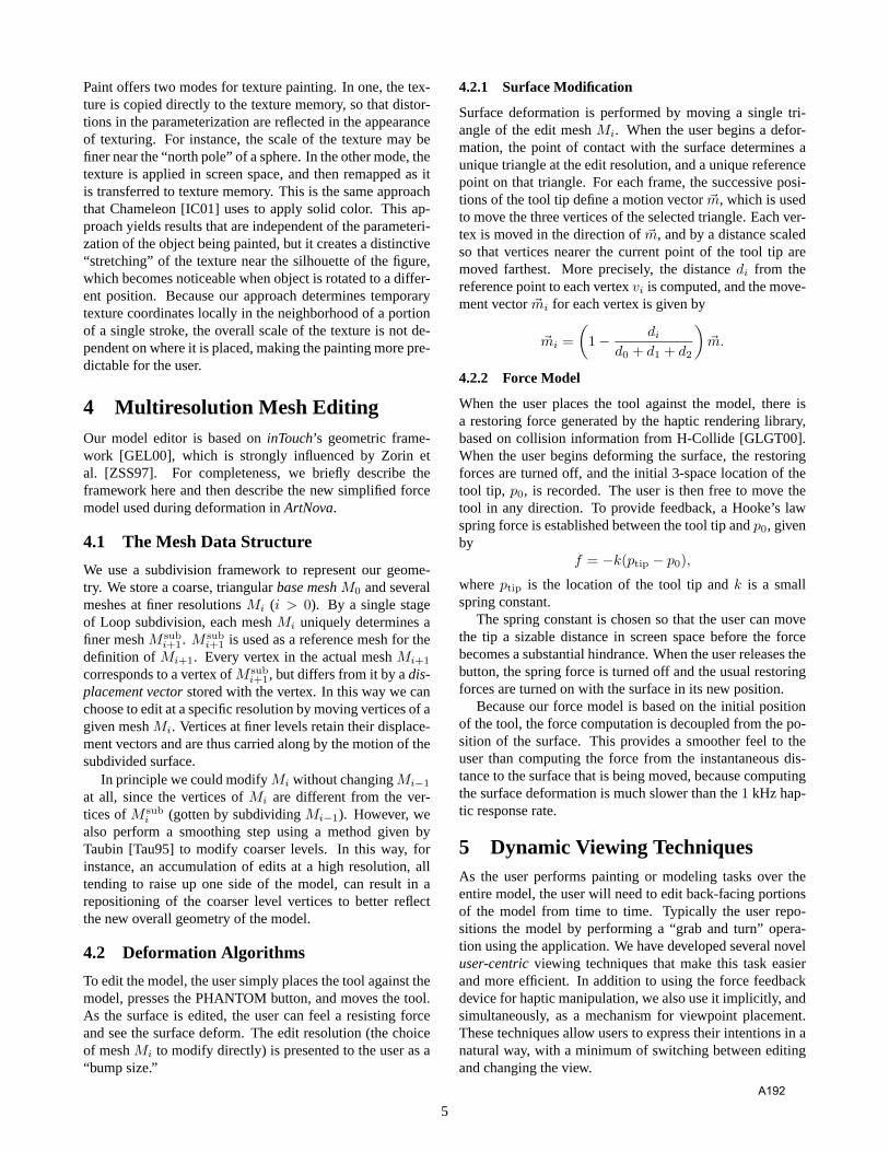
Paint offers two modes for texture painting. In one, the tex-ture is copied directly to the texture memory, so that distor-tions in the parameterization are reflected in the appearanceof texturing. For instance, the scale of the texture may befiner near the “north pole” of a sphere. In the other mode, thetexture is applied in screen space, and then remapped as itis transferred to texture memory. This is the same approachthat Chameleon [IC01] uses to apply solid color. This ap-proach yields results that are independent of the parameteri-zation of the object being painted, but it creates a distinctive“stretching” of the texture near the silhouette of the figure,which becomes noticeable when object is rotated to a differ-ent position. Because our approach determines temporarytexture coordinates locally in the neighborhood of a portionof a single stroke, the overall scale of the texture is not de-pendent on where it is placed, making the painting more pre-dictable for the user.
4 Multiresolution Mesh EditingOur model editor is based oninTouch’s geometric frame-work [GEL00], which is strongly influenced by Zorin etal. [ZSS97]. For completeness, we briefly describe theframework here and then describe the new simplified forcemodel used during deformation inArtNova.
4.1 The Mesh Data Structure
We use a subdivision framework to represent our geome-try. We store a coarse, triangularbase meshM0 and severalmeshes at finer resolutionsMi (i > 0). By a single stageof Loop subdivision, each meshMi uniquely determines afiner meshM sub
i+1. M subi+1 is used as a reference mesh for the
definition ofMi+1. Every vertex in the actual meshMi+1
corresponds to a vertex ofM subi+1, but differs from it by adis-
placement vectorstored with the vertex. In this way we canchoose to edit at a specific resolution by moving vertices of agiven meshMi. Vertices at finer levels retain their displace-ment vectors and are thus carried along by the motion of thesubdivided surface.
In principle we could modifyMi without changingMi−1
at all, since the vertices ofMi are different from the ver-tices ofM sub
i (gotten by subdividingMi−1). However, wealso perform a smoothing step using a method given byTaubin [Tau95] to modify coarser levels. In this way, forinstance, an accumulation of edits at a high resolution, alltending to raise up one side of the model, can result in arepositioning of the coarser level vertices to better reflectthe new overall geometry of the model.
4.2 Deformation Algorithms
To edit the model, the user simply places the tool against themodel, presses the PHANTOM button, and moves the tool.As the surface is edited, the user can feel a resisting forceand see the surface deform. The edit resolution (the choiceof meshMi to modify directly) is presented to the user as a“bump size.”
4.2.1 Surface Modification
Surface deformation is performed by moving a single tri-angle of the edit meshMi. When the user begins a defor-mation, the point of contact with the surface determines aunique triangle at the edit resolution, and a unique referencepoint on that triangle. For each frame, the successive posi-tions of the tool tip define a motion vector~m, which is usedto move the three vertices of the selected triangle. Each ver-tex is moved in the direction of~m, and by a distance scaledso that vertices nearer the current point of the tool tip aremoved farthest. More precisely, the distancedi from thereference point to each vertexvi is computed, and the move-ment vector~mi for each vertex is given by
~mi =(
1− did0 + d1 + d2
)~m.
4.2.2 Force Model
When the user places the tool against the model, there isa restoring force generated by the haptic rendering library,based on collision information from H-Collide [GLGT00].When the user begins deforming the surface, the restoringforces are turned off, and the initial 3-space location of thetool tip, p0, is recorded. The user is then free to move thetool in any direction. To provide feedback, a Hooke’s lawspring force is established between the tool tip andp0, givenby
f = −k(ptip − p0),
whereptip is the location of the tool tip andk is a smallspring constant.
The spring constant is chosen so that the user can movethe tip a sizable distance in screen space before the forcebecomes a substantial hindrance. When the user releases thebutton, the spring force is turned off and the usual restoringforces are turned on with the surface in its new position.
Because our force model is based on the initial positionof the tool, the force computation is decoupled from the po-sition of the surface. This provides a smoother feel to theuser than computing the force from the instantaneous dis-tance to the surface that is being moved, because computingthe surface deformation is much slower than the1 kHz hap-tic response rate.
5 Dynamic Viewing TechniquesAs the user performs painting or modeling tasks over theentire model, the user will need to edit back-facing portionsof the model from time to time. Typically the user repo-sitions the model by performing a “grab and turn” opera-tion using the application. We have developed several noveluser-centricviewing techniques that make this task easierand more efficient. In addition to using the force feedbackdevice for haptic manipulation, we also use it implicitly, andsimultaneously, as a mechanism for viewpoint placement.These techniques allow users to express their intentions in anatural way, with a minimum of switching between editingand changing the view.
5
A192

Our approach to the problem is to reposition the camerabased on the configuration (i.e. position and orientation) ofthe haptic probe so that the region of interest on the modelsurface is placed at the center of the view. We call our tech-niques “user-centric” because the haptic tool indicates wherethe user wants to view the object from, rather than where theobject should be.
5.1 Grabbing Operation
In the typical grabbing operation [RH92], the object ismoved preserving the transformation between the virtualprobe and the grabbing point. At the instant of grabbing, twopoints are picked:A, a point in the object, andB, the cur-rent position of the virtual probe. The transformationTBAfrom the probe to the object is set constant as the virtualprobe moves. Therefore, a displacement of the probe,∆TB ,produces a displacement of the object,∆Tg.
TBA = TA TB−1,
∆Tg = TBA ∆TB TBA−1.
whereTA andTB are the transformations that represent thelocation and orientation of the object and the virtual probe.
5.2 Viewpoint Navigation
We introduce a new concept called “viewpoint navigation”.This functionality is based on moving the viewpoint aroundthe object to be modeled or painted, based on the gestures ofthe user. The position and orientation of the haptic device ateach time are used as “commands”, which set a transforma-tion,Tn, on the position of the virtual probe and the camera,as shown in Fig. 6.
In our system we apply the inverse transformation to theobject that is being manipulated, producing the same visualeffect. In addition, we apply this transformation incremen-tally, whenever the viewpoint navigation is enabled.
∆Tn = K ∆TH .
where∆TH represents the variation of the position and ori-entation of the haptic device.
Figure 6. Viewpoint navigation based on user’sintentions.
5.3 Automatic Repositioning
Another novel functionality calledautomatic repositioningallows the user to reorient the model quickly without inter-rupting the work flow to change tools. When the automaticrepositioning key is pressed, the last point touched on themodel is taken to define the region of interest. A transfor-mationTr is computed that moves the camera to a locationalong the normal direction of the object at the point of inter-est (as shown in Fig. 7). Then, we apply the inverse transfor-mation to the object incrementally, so that the object appearsto rotate to the new position.
Figure 7. Automatic repositioning of viewpoint.
5.4 Combining all the Functionalities
The transformation that sets the location and orientation ofthe object is updated every time step for better viewing toaid the model manipulation and editing tasks, depending onwhich functionality is enabled. We have:TA,k+1 = ∆Tg TA,k, if grabbing is enabled;TA,k+1 = ∆Tn−1 TA,k, if viewpoint navigation is enabled;TA,k+1 = ∆Tr−1 TA,k, if automatic repositioning is en-abled.
6 ResultsWe have designed and implementedArtNovaas a proof-of-concept prototype system. In this section, we demonstratethe system capability and discuss issues related to the userinterface design.
6.1 Prototype Demonstration
We use a dual-processor Pentium III PC as a haptic server,a SensAble Technologies’ PHANTOM as a haptic device, aSilicon Graphics Inc. R12000 Infinite Reality for rendering,a large screen with a back projection system for graphicaldisplay, and UNC’s VRPN library [VRPN] for a network-transparent interface between application programs and ourhaptic system. The system is written in C++ using theOpenGL and GLUT libraries. However, the design frame-work of our system is applicable to all types of haptic de-vices and libraries, as well as graphical display and comput-ing platforms.
Several users with little or no experience in using model-ing or painting systems were able to create interesting mod-els usingArtNovawith little training. Each user was given
6
A193

Figure 8. A tree.
a selection of simple base meshes of various shapes (e.g.spherical, toroidal, etc.) and light gray in color. A few ex-amples of their art work are given in Figures 1, 3, 8, and 9.
The accompanying videotape illustrates a few examplesof the modeling and painting operations performed usingArtNova. Along with some more images of the models cre-ated by our users, the video clips are also available at:
http://www.cs.unc.edu/∼geom/ArtNova.
6.2 User Experiences
We have asked several users to evaluate our system by cre-ating and texture-painting a few models. We briefly summa-rize some of their comments here:
• The spring-based force model feels natural. Comparingthe experiences of performing model deformation withand without the physically-based force model, most ofthe users found the newly added force model to be animprovement.
• The users commented that the force feedback was use-ful in detecting and maintaining contact with the modelsurfaces, when performing highly detailed painting.
• Users also felt that texture painting was easy to use, andhad little trouble getting visually pleasing results.
• Users found automatic viewpoint adjustment and repo-sitioning to be intuitive and natural.
• The overall graphical user interface with our new 3Dtool metaphor was found to be intuitive and easy to un-derstand.
Figure 9. A fish.
7 SummaryWe have presented an integrated system for 3D texture paint-ing and multiresolution modeling with a haptic interface anduser-centric viewing. An artist or a designer can use this sys-tem to create and refine a three-dimensional multiresolutionpolygonal mesh, and further enhance its appearance by di-rectly painting textures onto its surface. The system allowsusers to naturally create complex forms and patterns aidednot only by visual feedback but also by their sense of touch.Based on preliminary user feedback, we believe these fea-tures considerably improve the ease and expressiveness of3D modeling and texture painting. We are currently plan-ning an extensive, formal user study to carefully evaluateand assess the contribution of various elements of this sys-tem on enhancing users’ experiences in digital model design.
8 AcknowledgmentsThis research is supported in part by a fellowship of the Gov-ernment of the Basque Country, NSF DMI-9900157, NSFIIS-9821067, ONR N00014-01-1-0067 and Intel. We wouldlike to thank the following individuals for their suggestionand assistance: Arthur Gregory, Stephen Ehmann, MichaelRosenthal, Adrian Ilie, Sarah Hoff, Bryan Crumpler, DerekHartman, Scott Cooper, and Joohi Lee.
References[ABL95] Maneesh Agrawala, Andrew C. Beers, and Marc Levoy. 3D
painting on scanned surfaces. In Pat Hanrahan and JimWinget, editors,1995 Symposium on Interactive 3D Graphics,pages 145–150. ACM SIGGRAPH, April 1995.
[AS96] R. S. Avila and L. M. Sobierajski. A haptic interaction methodfor volume visualization. Proceedings of Visualization’96,pages 197–204, 1996.
[BVIG91] Chakib Bennis, Jean-Marc Vezien, Gerard Iglesias, and AndreGagalowicz. Piecewise surface flattening for non-distortedtexture mapping. In Thomas W. Sederberg, editor,ComputerGraphics (SIGGRAPH ’91 Proceedings), volume 25, pages237–246, July 1991.
[CMS88] Michael Chen, S. Joy Mountford, and Abigail Sellen. A studyin interactive 3-D rotation using 2-D control devices. In JohnDill, editor, Computer Graphics (SIGGRAPH ’88 Proceed-ings), volume 22, pages 121–129, August 1988.
7
A194

[COR00] COREL. Painter.http://newgraphics.corel.com/products/painter6.html, 2000.
[DKT98] T. DeRose, M. Kass, and T. Troung. Subdivision surfaces incharacter animation.Proc. of ACM SIGGRAPH, 1998.
[FB88] D. Forsey and R.H. Bartels. Heirarchical B-spline refinement.In Proc. of ACM Siggraph, pages 205–212, 1988.
[GEL00] A. Gregory, S. Ehmann, and M. C. Lin.inTouch: Interactivemultiresolution modeling and 3d painting with a haptic inter-face.Proc. of IEEE VR Conference, 2000.
[GH91] Tinsley A. Galyean and John F. Hughes. Sculpting: An inter-active volumetric modeling technique. In Thomas W. Seder-berg, editor,Computer Graphics (SIGGRAPH ’91 Proceed-ings), volume 25, pages 267–274, July 1991.
[Gib95] S. Gibson. Beyond volume rendering: Visualization, hapticexploration, and physical modeling of element-based objects.In Proc. Eurographics workshop on Visualization in ScientificComputing, pages 10–24, 1995.
[GLGT00] A. Gregory, M. Lin, S. Gottschalk, and R. Taylor. Real-timecollision detection for haptic interaction using a 3-dof forcefeedback device.Computational Geometry: Theory and Ap-plications, Special Issue on Virtual Environments, 15(1-3):pp.69–89, February 2000.
[GW92] Michael Gleicher and Andrew Witkin. Through-the-lens cam-era control. In Edwin E. Catmull, editor,Computer Graphics(SIGGRAPH ’92 Proceedings), volume 26, pages 331–340,July 1992.
[HCT+97] J. Hollerbach, E. Cohen, W. Thompson, R. Freier, D. Johnson,A. Nahvi, D. Nelson, and T. Thompson II. Haptic interfacingfor virtual prototyping of mechanical CAD designs.CDROMProc. of ASME Design for Manufacturing Symposium, 1997.
[HDD+94] H. Hoppe, T. DeRose, T. Duchamp, M. Halstead, H. Jin,J. McDonald, J. Schweitzer, and W. Stuetzle. Piecewisesmooth surface reconstruction. InProceedings of ACM SIG-GRAPH, pages 295–302, 1994.
[Hem00] Right Hemisphere. Deep paint.http://www.us.deeppaint.com/,2000.
[HH90] Pat Hanrahan and Paul E. Haeberli. Direct WYSIWYG paint-ing and texturing on 3D shapes. In Forest Baskett, editor,Com-puter Graphics (SIGGRAPH ’90 Proceedings), volume 24,pages 215–223, August 1990.
[IC01] T. Igarashi and D. Cosgrove. Adaptive unwrapping for interac-tive texture painting.Proc. of ACM Symposium on Interactive3D Graphics, pages 209–216, 2001.
[JTK+99] D. Johnson, T. V. Thompson II, M. Kaplan, D. Nelson, andE. Cohen. Painting textures with a haptic interface.Proceed-ings of IEEE Virtual Reality Conference, 1999.
[KS99] A. Khodakovsky and P. Schroder. Fine level feature editingfor subdivision surfaces.Proceedings of ACM Symposium onSolid Modeling and Applications, 1999.
[Mas98] Thomas Massie. A tangible goal for 3D modeling.IEEE Com-puter Graphics and Applications, May/June, 1998.
[MQW01] K. McDonnell, H. Qin, and R. Wlodarczyk. Virtual clay: Areal-time sculpting system with haptic interface.Proc. of ACMSymposium on Interactive 3D Graphics, pages 179–190, 2001.
[MRF+96] William Mark, Scott Randolph, Mark Finch, James Van Verth,and Russell M. Taylor II. Adding force feedback to graphicssystems: Issues and solutions. In Holly Rushmeier, editor,SIGGRAPH 96 Conference Proceedings, Annual ConferenceSeries, pages 447–452, 1996.
[MS94] T. M. Massie and J. K. Salisbury. The phantom haptic inter-face: A device for probing virtual objects.Proc. of ASMEHaptic Interfaces for Virtual Environment and TeleoperatorSystems, 1:295–301, 1994.
[MYV93] Jerome Maillot, Hussein Yahia, and Anne Verroust. Interactivetexture mapping. In James T. Kajiya, editor,Computer Graph-ics (SIGGRAPH ’93 Proceedings), volume 27, pages 27–34,August 1993.
[OL01] M. Otaduy and M. Lin. User-centric viewpoint computationfor haptic exploration and manipulation.Proc. of IEEE Visu-alization, 2001. To appear.
[PBG92] C. Phillips, N. Badler, and J. Granieri. Automatic viewingcontrol for 3D direct manipulation.Proc. of ACM Symposiumon Interactive 3D Graphics, pages 71–74, 1992.
[PF01] R. Perry and S. Friskin. Kizamu: A system for sculpting dig-ital characters.Computer Graphics (ACM SIGGRAPH’01),2001.
[PFC+97] J. Pierce, A. Forsberg, M. Conway, S. Hong, R. Zeleznik, andM. Mine. Image plane interaction techniques in 3D immersiveenvironments. Proc. of ACM Symposium on Interactive 3DGraphics, pages 39–44, 1997.
[PFH00] E. Praun, A. Finkelstein, and H. Hoppe. Lapped textures.Proc. of ACM SIGGRAPH, pages 465–470, 2000.
[PT97] L. A. Piegl and W. Tiller.The NURBS Book. Springer Verlag,1997. 2nd Edition.
[QT96] Hong Qin and Demetri Terzopoulos. D-NURBS: A physics-Based framework for geometric design.IEEE Transactionson Visualization and Computer Graphics, 2(1):85–96, March1996. ISSN 1077-2626.
[RE99] A. Raviv and G. Elber. Three dimensional freeform sculptingvia zero sets of scalar trivariate functions.ACM Symposiumon Solid Modeling and Applications, 1999.
[RH92] Warren Robinett and Richard Holloway. Implementation offlying, scaling, and grabbing in virtual worlds. In DavidZeltzer, editor,Computer Graphics (1992 Symposium on In-teractive 3D Graphics), volume 25, pages 189–192, March1992.
[RKK97] D.C. Ruspini, K. Kolarov, and O. Khatib. The haptic display ofcomplex graphical environments.Proc. of ACM SIGGRAPH,pages 345–352, 1997.
[SP86] Thomas W. Sederberg and Scott R. Parry. Free-form defor-mation of solid geometric models. In David C. Evans andRussell J. Athay, editors,Computer Graphics (SIGGRAPH ’86Proceedings), volume 20, pages 151–160, August 1986.
[ST99] SensAble Technologies Inc.freeformTM modeling sys-tem. http://www.sensable.com/freeform, 1999.
[SZ98] P. Schroder and D. Zorin. Subdivision for modeling and ani-mation.ACM SIGGRAPH Course Notes, 1998.
[SZMS98] T. Sederberg, J. Zheng, M.Sabin, and D. Sewell. Non-uniformrecursive subdivision surfaces.Computer Graphics (ACMSIGGRAPH’98), 1998.
[Tau95] Gabriel Taubin. A signal processing approach to fair sur-face design. In Robert Cook, editor,SIGGRAPH 95 Confer-ence Proceedings, Annual Conference Series, pages 351–358.ACM SIGGRAPH, Addison Wesley, August 1995. held in LosAngeles, California, 06-11 August 1995.
[VRPN] Virtual Reality Peripheral Network.http://www.cs.unc.edu/research/nano/manual/vrpn.
[Wer94] Josie Wernecke.The Inventor Mentor. Addison-Wesley, 1994.
[WO90] C. Ware and S. Osborne. Exploration and virtual camera con-trol in virtual three dimensional environments.Proc. of ACMSymposium on Interactive 3D Graphics, pages 175–183, 1990.
[ZF99] Robert Zeleznik and A. Forsberg. Unicam 2D gestural cameracontrols for 3D environments.Proc. of ACM Symposium onInteractive 3D Graphics, pages 169–173, 1999.
[ZSS97] D. Zorin, P. Schroder, and W. Sweldens. Interactive mul-tiresolution mesh editing.Computer Graphics (ACM SIG-GRAPH’97), 1997.
8
A195


RECENT ADVANCES IN HAPTIC RENDERING AND APPLICATIONS Supplementary Course Notes PART II – Presentation Slides Ming C. Lin University of North Carolina at Chapel Hill Miguel A. Otaduy ETH Zurich
B1

B2

Course: Recent Advances in Haptic Rendering and Applications
Introduction and Overview
Miguel A. Otaduy
ETH-Zurich
http://graphics.ethz.ch/~otmiguel
Ming C. Lin
UNC-Chapel Hill
http://www.cs.unc.edu/~lin
DefinitionDefinition
Haptic Rendering: display of information through force or tactile cues.
Visual Display
Auditory Feedback
Haptic RenderingIntuitive interactionwith virtual environmentsIncrease presence
HistoryHistory
• Used in master-slave telerobotic systems
• First suggested by Sutherland [1965] for interaction with VEs
• Project GROPE in UNC:– 2D force field simulation [1971]
– 3D molecular docking [1990]
HistoryHistory
• [Minsky et al. 1990]: rendering of 2D textures.
2D height field
2DOF device
Compute Fx, Fyforces using
gradients
HistoryHistory
• [Zilles and Salisbury 1995; Ruspini et al. 1997]: point-object interaction.
Object, point (p) and proxy (x)
p
x
Constrain x to the surface
Force given by dist(x,p)
3DOF device
HistoryHistory
• [McNeely et al. 1999]: interaction between rigid objects. Also called 6DOF haptic rendering.
Sample objects
Per-sample collision test
Net force and torque
6DOF device
B3

Description of the ProblemDescription of the Problem
1. Move grabbed object according to input
2. Compute contact forces between objects
3. Apply net force and torque to grabbed object
Similar to Rigid Body Simulation
Description of the ProblemDescription of the Problem
• Control engineering analysis:
ActuatorsUserControl
Device +Biomechanics
HapticRendering
F1 F*F2
F
Pos*
Pos
Pos
Description of the ProblemDescription of the Problem
• Control engineering analysis:
ActuatorsUserControl
Device +Biomechanics
HapticRendering
F1 F*F2
F
Pos*
Pos
Pos
active
Description of the ProblemDescription of the Problem
• Control engineering analysis:
ActuatorsUserControl
Device +Biomechanics
HapticRendering
F1 F*F2
F
Pos*
Pos
Pos
Human-in-the-looppassive
Description of the ProblemDescription of the Problem
• Control engineering analysis:
• High sensitivity to instabilities!!
• High update rates required!! (kHz for high stiffness)
ActuatorsUserControl
Device +Biomechanics
HapticRendering
F1 F*F2
F
Pos*
Pos
Pos
Human-in-the-loop
Description of the ProblemDescription of the Problem
• 2 major components:– Collision detection / contact determination
– Contact response model and force computation
B4

Course: Recent Advances in Haptic Rendering and Applications
Session I: Design Guidelines and Basic Point-Based Techniques
Haptic Perception andImplications for Design
Roberta Klatzky
Carnegie Mellon UniversityDept. of Psychology
Human-Computer Interaction Institute
Center for the Neural Basis of Cognition
Haptic Perceptionand implications for designHaptic Perceptionand implications for design
• What is haptic perception?
• Based on touch receptors• in skin, muscles, tendons, joints
• Usually involves active seeking of information (exploration)
Outline of TalkOutline of Talk
• Neural Coding of Touch Primitives
• Functions of Peripheral Receptors
• Haptic Primitives and their Encoding
• Complementary Functions of Haptics and Vision
• Emergent Issues for Design
1. Neural Coding of Touch Primitives1. Neural Coding of Touch Primitives
• Touch Receptors– Mechanoreceptors and their Function
– Other skin receptors: thermal, pain
• Pathways from receptors to brain
Touch ReceptorsTouch Receptors
• Touch sensations are mediated by receptors that respond to pressure, vibration, and heat flow.
• The receptors are found in two regions:
-- Within skin: cutaneous sensing pressure, temperature, pain
-- Beneath skin in muscles, tendons, joints:
kinesthetic sensinglimb position and movement
Classes of ReceptorsClasses of Receptors
• Receptors that respond to pressure and vibration are called mechanoreceptors
• Mechanoreceptors are found in skin (cutaneous) and muscles, tendons, and joints (kinesthesis)
• The skin also includes other receptors – that signal skin warming and cooling (thermo-receptors)
– that signal pain (nociceptors)
B5

Skin Mechanoreceptors have specialized endingsSkin Mechanoreceptors have specialized endings
Meissner
Merkel
Ruffini
Pacinian
Fast adapting Type I
Slow adapting Type I
Slow adapting Type II
Fast adapting Type II
Functional Name:
Johannson & Valbo, 1983
Functional characteristics of Skin Mechanoreceptors:Receptive field size and adaptation rateFunctional characteristics of Skin Mechanoreceptors:Receptive field size and adaptation rate
Kandel et. al., 2000
Meissner’s Merkel Pacinian RuffiniCorpuscle Cell Complex Corpuscle Ending
Receptors
Receptive
Field
Intensity and Time Course of Neural Signal (adaptation)
NeuralSpike train
Stimulus
FA I SA I FA II SA II
Frequency Sensitivity: One-channel-per-mechanoreceptor modelFrequency Sensitivity: One-channel-per-mechanoreceptor model
Amplituderequiredfor a threshold response, at a given frequency(dB relative to 1 µm)
Bolanowski et al., 1988
Thermal ReceptorsThermal Receptors
Thermo-receptors lack specialized endings. Two populations of nerve fibers: warm and cold
Each has its own response range, with some overlap. Note: body temperature in Centigrade = 37º.
Neural response rate
20 25 30 35 40 45 50Temperature ( C )
Cold Warm
Kenshalo, 1976
A variety of neural fibers lead from periphery to spinal cord.A variety of neural fibers lead from periphery to spinal cord.
Fiber Speed Associated receptors
A-α fast kinesthetic
A-β moderately fast kinesthesthetic & cutaneous mechano.
A-δ moderately fast thermo- & nociceptor (sharp pain)
C slow thermo- & nociceptor (burning pain)
4 types, varying in conduction speed and associated receptor populations
Two pathways from cord to the brainTwo pathways from cord to the brain
Slow, oldFast, new
Cutaneous, Nociceptor, thermal, kinesthetic some mechanoreceptorsUnidentified source
B6

The brain: Primary and Secondary Somatosensory CortexThe brain: Primary and Secondary Somatosensory Cortex
SI
SII
Areas 5,7SI includes Brodmann areas:3a: Muscle3b: Skin (SA and FA)1: Skin (FA)2: Pressure, joints
SI projects to SII, 5, 7
SISII
Motor
Somatosensory “Homunculus” in SIresults from somatotopic mapping*Somatosensory “Homunculus” in SIresults from somatotopic mapping*
*Adjacent on skin⇒Adjacent in SI
There are severalsuch maps.
Penfield & Rasmussan, 1950
Somatosensory areas in brain are plastic: Re-assignment of receptive fields after amputation of a digit
Somatosensory areas in brain are plastic: Re-assignment of receptive fields after amputation of a digit
Areas in SI that once responded to 3rd fingertip are now activated by finger 2 and 4, plus base of 3
Merzenich et al., 1984
2. Functions of peripheral receptors
2. Functions of peripheral receptors
• Cutaneous mechanoreceptors provide array (tactile) sensing.
• Kinesthetic mechanoreceptors provide a sense of limb position, movement.
• They support different human abilities.
Grasping is supported by FAI mechanoreceptors that detect incipient slip
Grasping is supported by FAI mechanoreceptors that detect incipient slip
Under near slip conditionsGrasp, lift… Return
Load Force N
Grip Force N
Position mm
Grip: Load ratio
Time
Load Force N
Grip Force N
Position mm
Force Ratio
FA ISA IFA IISA II
Slip threshold
Johansson & Westling, 1984; Westling, 1986
Tactile Pattern Perception is based on SA I mechanoreceptorsTactile Pattern Perception is based on SA I mechanoreceptors
Input pattern
Response
Phillips, Johansson & Johnson, 1990
Spatial plot of the response of a skin mechanoreceptor to a Braille pattern swept through its receptive field: Each tick mark is a neural impulse given contact from that stimulus location. SA I have resolution of ~.5 mm at fingertip.
PatternpreservationSA I
FA I
SA II
FA II
B7

Curvature perception also reflects SA I responsesCurvature perception also reflects SA I responses
-4 -2 0 2 4Distance of receptive field from center of indentation (mm)
MeanSA IResponse
Data are shown for 7 curves, ranging from radius zero to radius 1.44 mm
Goodwin et al., 1995
Roughness perception is directly related to spatial variation in SA I responses
Roughness perception is directly related to spatial variation in SA I responses
SubjectiveRoughnessMagnitude
Mean impulse rate (impulses/s)0 25 50 75 100 0 25 50 75 1000 25 50 75 100
Spatial variation in impulse rate (impulses/s)0 25 50 75 100 0 20 40 80 0 25 50
SAI RA PC
Note: large roughness range for a single mean
Connor, Hsaio, Phillips, Johnson, 1990
Mean impulse rate does not predict roughness magnitude.
What do PC receptors signal?What do PC receptors signal?
• Anything that causes deep vibrations
-- Transient vibrations from contact
-- Micron-element textural variations
Only PCs respond continuously to thetextured portion of a half-textured platewith ht. 1 µm
Srinivasan, Whitehouse, & LaMotte, 1990
Kinesthetic mechanoreceptors are involved in softness perceptionKinesthetic mechanoreceptors are involved in softness perception
Softness discrimination of rubber specimens vs. rigidly covered springs
• Pure kinesthesis condition: anesthetize fingertips -- no cutaneous cues• Pure cutaneous condition: passively press stimulus against fingerpad
-- no muscle/tendon/joint involvement• Dual-cue condition: normal, active touch
• Deformable surface (rubber) could be judged from cutaneous cues alone.• Rigid (spring-loaded) surfaces required kinesthesis + cutaneous cues.
Srinivasan & LaMotte, 1995
3. Haptic primitives and their encoding3. Haptic primitives and their encoding
• Haptically perceived properties of objects and surfaces
• Link between exploration and perception of haptic properties
What are haptically perceptible properties of objects?What are haptically perceptible properties of objects?
• Geometry: Size (2-D, 3-D), Shape, Pointiness..
• Surface: Roughness, Slipperiness, Warmth…
• Substance: Compliance, Weight
B8
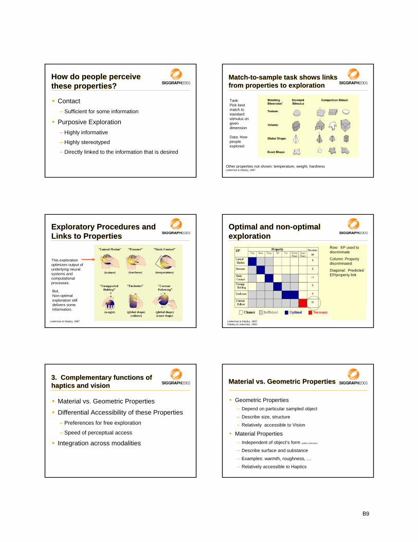
How do people perceive these properties? How do people perceive these properties?
• Contact– Sufficient for some information
• Purposive Exploration– Highly informative
– Highly stereotyped
– Directly linked to the information that is desired
Match-to-sample task shows links from properties to explorationMatch-to-sample task shows links from properties to exploration
Other properties not shown: temperature, weight, hardnessLederman & Klatzky, 1987
Task:Pick best match to standard stimulus on given dimension
Data: How people explored
Exploratory Procedures and Links to PropertiesExploratory Procedures and Links to Properties
This exploration optimizes output of underlying neural systems and computational processes.
But, Non-optimal exploration still delivers some information.
Lederman & Klatzky, 1987
Optimal and non-optimal explorationOptimal and non-optimal exploration
Row: EP used to discriminate
Column: Property discriminated
Diagonal: Predicted EP/property link
Lederman & Klatzky, 1987; Klatzky & Lederman, 1993
3. Complementary functions of haptics and vision3. Complementary functions of haptics and vision
• Material vs. Geometric Properties
• Differential Accessibility of these Properties– Preferences for free exploration
– Speed of perceptual access
• Integration across modalities
Material vs. Geometric PropertiesMaterial vs. Geometric Properties
• Geometric Properties– Depend on particular sampled object
– Describe size, structure
– Relatively accessible to Vision
• Material Properties– Independent of object’s form (within extremes)
– Describe surface and substance
– Examples: warmth, roughness, …
– Relatively accessible to Haptics
B9

Preferences under free exploration with vision and touchPreferences under free exploration with vision and touch
• Subjects asked, which of two objects is rougher, harder…
• Some questions were easy (roughness of sandpaper vs. silk), some difficult (size of golf ball vs. marshmallow)
0
20
40
60
80
100
Rou
gh
Har
d
Tem
p
Wei
ght
Size
Shap
eDimension
Mea
n pe
rcen
t tou
ched Difficult
Easy
Klatzky, Lederman, & Matula 1993
Touch is used fordifficult judgments of material properties.
Otherwise, vision used for perceptual comparison or to trigger memory retrieval.
Speed of access to properties by touch favors material over geometry
Speed of access to properties by touch favors material over geometry
• Subjects search for a target object presented to one finger, while other fingers get 0-5 distractors
Lederman & Klatzky, 1997; apparatus developed at Queen’s University
Speed of access, continuedSpeed of access, continued
• Judgments of several types of properties
Material
Edge content
Spatial RelationsLederman & Klatzky, 1997
Speed of access, continuedSpeed of access, continued
Increasing slope indicates finger by finger search: characteristic of spatial queries
Flat slope indicates target “pops out”: characteristic of material, edge queriesNumber fingers stimulated
Lederman & Klatzky, 1997
Haptic/visual integrationHaptic/visual integration
• If material properties are relatively accessible to touch,
• And geometric properties are relatively accessible to vision,
• How do the two modalities interact?
• Apparently -- often -- optimally!– Ernst and Banks
Maximum Likelihood ModelMaximum Likelihood Model
• Vision, touch assumed to input to a common integrator
• Integrator weights signals by reliability: inversely related to variance
• Integrator adds weighted signals
B10

Applying the model to roughness perceptionApplying the model to roughness perceptionVisual input from stereo gogglesNoise added by eliminating stereo from some locations
Haptic input from PHANTOM force feedback device
Results: Optimal weighting of vision, depending on noise
Ernst & Banks, 2002
5. Emergent Issues for Design5. Emergent Issues for Design
• Implications of encoding pathways
• Implications of intersensory integration
• The “holy grail” of haptic interface design
Implications of hapticencoding pathwaysImplications of hapticencoding pathways• Multiple receptors enable touch to encode a variety
of neural primitives– A map of deformation on the fingertip
– Vibration, skin stretch, temperature
– Also enable fine manipulation
• Peripheral primitives, combined with active exploration, richly depict objects and surfaces– Haptics favors material over geometry
– Haptics and Vision are complementary
Implications of intersensoryintegrationImplications of intersensoryintegration• Inputs from other sensory systems are integrated
with haptics• Integration is sensitive to sensory reliability
– Vision can compensate for relatively coarse spatial coding by haptics
– Haptics can compensate for relatively coarse material coding by vision
– One sense can be “fooled” by the other, • e.g., coarse visual textures make surfaces feel rougher;
• visual curves make haptic edges feel rounder
The “holy grail”The “holy grail”
• Not just your grandmother’s force-feedback device
• Need dense, robust, array stimulators
• Thermal stimulation highly useful
• Exploration should be maximally enabled
• Add other modalities to capitalize on human multi-sensory abilities
B11

Course: Recent Advances in Haptic Rendering and Applications
Session I: Design Guidelines and Basic Point-Based Techniques
Introduction to 3-DoFHaptic Rendering
Ming C. LinDepartment of Computer Science
University of North Carolina at Chapel Hill
http://www.cs.unc.edu/~lin
3DOF Haptics: Introduction3DOF Haptics: Introduction
• Output: 3D force 3DOF haptics• Limited to applications where point-object
interaction is enough.– Haptic visualization of data– Painting and sculpting– Some medical applications
Object-object
Point-object
3DOF Haptics: Basic approach3DOF Haptics: Basic approach
• Check if point penetrates an object.
• Find closest point on the surface.
• Penalty-based force.xF
xkF ⋅=
3DOF Haptics: The problems3DOF Haptics: The problems
• Force discontinuities when crossing boundaries of internal Voronoi cells.
F1
F2
Unexpected force discontinuities (both in
magnitude and direction) are very disturbing!
3DOF Haptics: The problems3DOF Haptics: The problems
• Pop-through thin objects.
After the mid line is crossed, the force helps
popping through.
motion
3DOF Haptics: Point-to-plane3DOF Haptics: Point-to-plane• Mark et al., 1996.• For distributed applications. The simulator sends
the equation of a plane to the haptic loop. The update of the plane is asynchronous.
• Forces are computed between the haptic point and the plane.
• Possible stiffness is limited, because too stiff would bring a jerky behavior at low update rates.
B12

3DOF Haptics: God-object3DOF Haptics: God-object
• Zilles and Salisbury, 1995.• Use the position of the haptic interface point
(HIP) and a set of local constraint surfaces to compute the position of god-object (GO).
• Constraint surfaces defined using heuristics.• Compute GO as the point that minimizes the
distance from HIP to the constraint surfaces. Lagrange multipliers.
3DOF Haptics: God-object3DOF Haptics: God-object
• Constraint surfaces:– Surfaces impeding motion
– GO is outside (orientation test) and in the extension of the surface.
– The HIP is inside the surface.
motion
edge/vertexConcavity: 2/3
constraint planes in 3D
motion
3DOF Haptics: God-object3DOF Haptics: God-object
• Constraint plane equations:
• Energy function that will account for the distance.
• Define cost function using Lagrange multipliers.
• Minimize, solving for x, y, z, λ1, λ2 and λ3.
0=+⋅+⋅+⋅ iiii DzCyBxA
( ) ( ) ( )( )222
21
HIPHIPHIP zzyyxxkE −+−+−⋅⋅=
3 planes at most
( ) ( ) ( )( )( )∑
=
+⋅+⋅+⋅⋅+
+−+−+−⋅⋅=
3
1
222
21
iiiiii
HIPHIPHIP
DzCyBxA
zzyyxxkC
λ
3DOF Haptics: God-object3DOF Haptics: God-object
• Partial derivatives on x, y, z, λ1, λ2 and λ3yield 6 linear equations:
• In case of less than 3 planes, the problem has a lower dimension.
⎟⎟⎟⎟⎟⎟⎟⎟
⎠
⎞
⎜⎜⎜⎜⎜⎜⎜⎜
⎝
⎛
=
⎟⎟⎟⎟⎟⎟⎟⎟
⎠
⎞
⎜⎜⎜⎜⎜⎜⎜⎜
⎝
⎛
⋅
⎟⎟⎟⎟⎟⎟⎟⎟
⎠
⎞
⎜⎜⎜⎜⎜⎜⎜⎜
⎝
⎛
3
2
1
3
2
1
333
222
111
321
321
321
000000000
100010001
DDD
zyx
zyx
CBACBACBA
CCCBBBAAA
HIP
HIP
HIP
λλλ
3DOF Haptics: Virtual proxy3DOF Haptics: Virtual proxy
• Ruspini et al., 1997.
• Based on god-object.
• Virtual proxy is a small sphere, instead of a point. Use configuration-space obstacles (C-obstacles), from robotics.
• More formal definition of constraint planes.
• Implementation of additional features, based on relocation of the virtual proxy.
3DOF Haptics: Virtual proxy3DOF Haptics: Virtual proxy
• C-obstacles: for a spherical object, is reduced to computing offset surfaces at a distance equal to the radius of the sphere.
• Check the HIP against the offset surface.
• This is done to avoid problems with small gaps in the mesh.
B13

3DOF Haptics: Virtual proxy3DOF Haptics: Virtual proxy
• Finding the virtual proxy is based on an iterative search.• Basically, find subgoals based on the same distance
minimization as for the god-object.• At each subgoal, all the planes that go through that point
are potential constraints. The minimum set of active constraints is selected.
• If the subgoal is in free space, set as new subgoal the HIP. The path might intersect the C-obstacles. Add the first plane intersected as a constraint and the intersection point as the current subgoal.
• The process ends when the virtual proxy becomes stable.
3DOF Haptics: Virtual proxy3DOF Haptics: Virtual proxyHIP(t)
Perform collision detection between the path of the HIP
and the C-obstacles
HIP(t+∆t)
3DOF Haptics: Virtual proxy3DOF Haptics: Virtual proxyHIP(t)
Set the subgoal and the constraint plane(s)
HIP(t+∆t)
3DOF Haptics: Virtual proxy3DOF Haptics: Virtual proxyHIP(t)
HIP(t+∆t)
Find a new subgoalusing the active planes and the minimization based on Lagrange
multipliers
3DOF Haptics: Virtual proxy3DOF Haptics: Virtual proxyHIP(t) Since the subgoal is in
free space, drop the constraints, set the HIP as
the new subgoal and perform collision
detection between the path and the C-obstacles
HIP(t+∆t)
3DOF Haptics: Virtual proxy3DOF Haptics: Virtual proxyHIP(t)
Recompute subgoalwith new constraints
HIP(t+∆t)
B14

3DOF Haptics: Virtual proxy3DOF Haptics: Virtual proxyHIP(t)
The path to the new subgoal intersects another plane, so
this is added to the set of constraints
HIP(t+∆t)
3DOF Haptics: Virtual proxy3DOF Haptics: Virtual proxyHIP(t) Compute active
constraints (in 2D there are only 2) and
find subgoal
HIP(t+∆t)
For this example, this is the final position of the virtual proxy
3DOF Haptics: Virtual proxy3DOF Haptics: Virtual proxy
• Quadratic programming approach:– The constraint planes define an open convex region
(bounded by the plane at infinity).
– The function to minimize is the distance from the hapticdevice (HIP) to the new subgoal (VPi+1):
– The translation from the current location to the new subgoal cannot intersect the constraint planes. Define linear constraints based on the normals of the planes.
Quadratic function)(1 ttHIPVPC i ∆+−= +
( ) 01 ≥−⋅ + iii VPVPN Linear constraints
3DOF Haptics: Virtual proxy3DOF Haptics: Virtual proxy
• Special case: simplified approach.– Let’s look at the convex region defined by the
constraint planes
Plane at ∞
Plane at ∞Plane at ∞
Plane at ∞
Vertex EdgeFace (all surrounded
by the plane at ∞)
3DOF Haptics: Virtual proxy3DOF Haptics: Virtual proxy
– Normals (n) become points (-n) in a dual space (Gauss map).
– The plane at infinity is the origin (o).– Points (-n) are joint together if the associated planes
intersect.– The position of the virtual proxy also has a dual:
– The vertices of the closest feature to P are the duals of the active constraint planes that are used for the minimization with Lagrange multipliers.
i
i
VPHIPVPHIPP
−−
=
3DOF Haptics: Virtual proxy3DOF Haptics: Virtual proxy
B15

3DOF Haptics: Virtual proxy3DOF Haptics: Virtual proxy
• Force output: PD (proportional- derivative) control. Produces a force that will try to keep the VP and the HIP at the same position.
User
SimulationVP
PD control ActuatorsF* F
HIP
( )dt
HIPVPdKHIPVPKF dp−
⋅+−⋅= )(*
It’s like a spring+damper, but the authors look at it from a
control engineering approach
3DOF Haptics: Additional features3DOF Haptics: Additional features• Force shading by Basdogan et al., 1997.
– Interpolate per-vertex normals using baricentriccoordinates
– Effect: edges and vertices seem ‘rounded’
A1A2
A3 v2v1
v3
''' 3
1
3
1
NNN
A
NAN
ii
iii
=⋅
=
∑
∑
=
=
3DOF Haptics: Additional Features3DOF Haptics: Additional Features• Force shading by Ruspini et al., 1997.
– Modify the position of the VP.– A subgoal (HIP’) is computed changing the
normal of the plane.– This subgoal replaces the HIP, and the final
VP is computed.
HIP
HIP’
VPOriginal plane
Force-shaded plane
3DOF Haptics: Additional Features3DOF Haptics: Additional Features
• Other effects by Ruspini et al., 1997.– Friction.
– Textures.
– Deformation.
• All of them are achieved performing operations that modify the position of the VP.
3DOF Haptics: Additional Features3DOF Haptics: Additional Features• Friction by Hayward and Armstrong, 2000.
– Model friction as an elasticity between the actual contact point (x) and a fictitious point, called adhesion point (w).
– The adhesion point remains static or follows the actual contact depending on the ‘state’ (sliding, static…) xw
3DOF Haptics: H-Collide3DOF Haptics: H-Collide
• What about the collision detection?– Spatial uniform decomposition of space. Locate the path
traversed by the probe in that grid, using a hash table.
– Test the path against an OBBTree. Optimized test.
– Use frame-to-frame coherence, caching the previous contact, and perform incremental computation.
– When the leaf intersects, compute the surface contact point (SCP). Pass this to GHOST (haptic rendering library used by the Phantoms).
B16

3DOF Haptics: H-Collide3DOF Haptics: H-Collide
Spatial partitioning with hash table Ray Vs. OBBTree test
SCP computationSCP
The EndThe End
For more information, see
http://gamma.cs.unc.edu/interactive
http://gamma.cs.unc.edu/HCollide
B17

Course: Recent Advances in Haptic Rendering and Applications
Session II: 6-DoF Haptic Rendering for Object-Object Interaction
Introduction to 6-DoFHaptic Display
Bill McNeely
Boeing Phantom Works
http://www.boeing.com/phantom
MotivationMotivation
• Why six degrees of freedom?– Allowable motions of an extended rigid object
– E.g., 3 Cartesian coordinates plus 3 Euler angles
• Basic to most real-world tasks– Virtual prototyping
– Training
Why is 6-DOF so difficult?Why is 6-DOF so difficult?
• Detect all contacts of interacting objects– Assume rigid bodies, but otherwise no a priori
constraints on shape or motion
• Calculate forces and torques– For hard contact / contact avoidance
• 1000+ Hz haptic update rate– 10+ Hz graphic update rate
Key decisionsKey decisions
• Collision Detection– Choice of representation and algorithm
• Interaction Paradigm– Penalty forces
– Virtual coupling
– Newtonian dynamics / Quasi-static approximation
– Single user vs. collaboration
Further decisionsFurther decisions
• Decouple haptic and simulation loops?– Use intermediate representations?
• Force type and quality– How hard does hard contact feel?
– How free does free-space feel?• Repulsive forces?
• Force artifacts / stability considerations
Three ApproachesThree Approaches
• Voxmap PointShell™ (VPS)– W. McNeely, K. Puterbaugh, and J. Troy
• Sensation-Preserving Simplification– M. Otaduy and M. Lin
• Spatialized Normal-Cone Hierarchies– D. Johnson and E. Cohen
B18

Course: Recent Advances in Haptic Rendering and Applications
Session II: 6-DoF Haptic Rendering for Object-Object Interaction
Voxel Sampling forSix-DoF Haptic Rendering
Bill McNeely
Boeing Phantom Works
http://www.boeing.com/phantom
VPS decisionsVPS decisions
• Voxel representation; Point-voxel sampling– 3-level 512-tree voxel hierarchy
• Voxels / chunks / hyperchunks
• Penalty forces; Virtual coupling
• Tactical degradation of force quality– Free-space viscosity artifact
• No decoupling of haptic and simulation loops
VPS collision detectionVPS collision detection
• Voxel sampling
VPS interaction paradigmVPS interaction paradigm
• Penalty Forces Virtual coupling
Some myths about VPSSome myths about VPS
• “Cannot simulate multiple moving objects”
• “Not scalable to large scenarios”
• “VPS videos betray a stability problem”
• (Your favorite myth here)
VPS progress since 1999VPS progress since 1999
• 40x improvement in spatial accuracy– Applied to the design of Boeing 777-300ER
• Collaborative haptics
• See “Advances in Voxel-Based 6-Dof HapticRendering”
B19

Geometrical Awareness (2D)Geometrical Awareness (2D)
• Vertex-edge contacts determine dynamically correct behavior of rigid polygons in 2D– “Edge” includes vertices
Geometrical Awareness (3D)Geometrical Awareness (3D)
• Vertex-surface and edge-edge contacts determine dynamically correct behavior of rigid polyhedra in 3D– “Surface” includes edges
– “Edge” includes vertices
Voxel Based Distance FieldsVoxel Based Distance Fields
• Voxels marked with distance-to-contact
• 3 types of fields: Surface, edge, vertex
Temporal CoherenceTemporal Coherence
• Anticipate force-generating collisions
• Sample fewer points using dead reckoning– Sampling rate varies inversely with distance-to-
contact
• Slow down the motion if necessary– Prime directive: Avoid undetected contacts!
– Accept a free-space viscosity artifact in trade
Distance-to-contact queuesDistance-to-contact queues
• Mark each point with distance-to-contact
• Order points into distance-specific queues– Points free to migrate between queues
• (Partially) traverse each queue every frame
• Extend this scheme to the voxel hierarchy– Hierarchical temporal coherence
MaxTravelMaxTravel
MaxTravel = (nCapacity – nMandatory) / Σ (ni / (0.5 voxelsize · i))
where:nCapacity = number of point-voxel tests CPU can perform in 1 msnMandatory = number of “mandatory” (contacting) pointsi = index of “discretionary” (non-contacting) queueni = number of points currently occupying queue i
Number of discretionary tests = MaxTravel · ni / (0.5 voxelsize · i)
Definition: Maximum allowable travel of any point during current frame
B20

What happens when nMandatory exceeds nCapacity?What happens when nMandatory exceeds nCapacity?
• Graceful degradation – If nMandatory exceeds (0.95 · nCapacity), then
test every mandatory point plus (0.05 · nCapacity) discretionary points
– Allow frame rate to fall below 1000 Hz• Hopefully the haptic interface tolerates this situation
• Add more processing power?– Or use a larger voxel size
Scalability characteristicsScalability characteristics
• CPU cycles per frame ~ O( 1/voxelsize2 )
• Amount of voxel data ~ O( 1/voxelsize3 )– O( 1/voxelsize2 ) at currently realistic voxel sizes
• Multiple moving objects– CPU cycles ~ O( nMovingObjects2 )
Large-scale VPS hapticsLarge-scale VPS haptics VPS-enabled FlyThru®VPS-enabled FlyThru®
• Client-server architecture
• 777-300ER main landing gear at ~1mm accuracy– 40,476 triangles moving (1.1 M points)
– 2.7M triangles static (1.8 G voxels)
• Dynamic pre-fetching of voxel data
– SensAble Technologies PHANTOM® 1.5/6DOF
– Bi-Xeon 2.8 GHz with 2 GB RAM
Engine exampleEngine example VPS-enabled CATIA®/Haption® prototypeVPS-enabled CATIA®/Haption® prototype
Interactive assembly simulation with force-feedbackinside CATIA V5
EuroHaptics 2004, Munich, Germany, June 5-7, 2004
Haptic device: Virtuose 6D35-45 by HaptionSoftware solution: Catia V5 R11 using VPS/PBM
CAD model: Courtesy of Renault
B21

CATIA/Haption demoCATIA/Haption demo
• 1.5mm voxel size
• 36,565 triangles static; 2,354 moving
• Voxelization time 1.5 minutes
• Bi-Xeon 2.4 GHz with 1 GB RAM
• Maximum force 35N, torque 3Nm
Collaborative 6-DOF hapticsCollaborative 6-DOF haptics
Collaborative 6-DOF HapticsCollaborative 6-DOF Haptics
• “Type 2” cross-user virtual coupling– Ensures stability regardless of latency
Virtual SwordplayVirtual Swordplay
Non-planar manifold contactNon-planar manifold contact Why is it a difficult scenario?Why is it a difficult scenario?
• Geometrical awareness loses effectiveness
• Extreme non-convexity is guaranteed
• Why not use formal kinematic constraints?– Tricky transitions between unilateral and quasi-
permanent constraints
– System complexity increases
B22

VPS experimental approachVPS experimental approach
• Allow slight surface interpenetration
• Retract pointshell slightly– E.g., by ½ voxel along inpointing surface normal
• Ball and socket example– At voxel size of (0.01 · diameter), MaxTravel allows
maximum rotational speed of 0.5 revolution/sec
B23

Course: Recent Advances in Haptic Rendering and Applications
Session II: 6-DoF Haptic Rendering for Object-Object Interaction
Sensation Preserving Simplification for 6-DoF Haptic Display
Miguel A. Otaduy
ETH-Zurich
http://graphics.ethz.ch/~otmiguel
OutlineOutline
• Motivation
• Sensation Preserving Simplification
• Multiresolution Collision Detection
• Rendering Pipeline
• Conclusion
Bottleneck: Collision DetectionBottleneck: Collision Detection
• Input:– Object A: m triangles Object B: n triangles
• Query:– Return all pairs of triangles closer than d
• Worst case scenario: O(mn)– Parallel close proximity (large areas closer than d)
• Desired force update rate ~1kHz
• Larger contact area Lower resolution
• Supported by studies on feature detection [Klatzky and Lederman 1995, Okamura and Cutkosky 1999]
Perceptual MotivationPerceptual Motivation
Goal: Adaptive ResolutionGoal: Adaptive Resolution
low res
high res
Goal: Adaptive ResolutionGoal: Adaptive Resolution
B24

Levels of DetailLevels of Detail
• Widely used in graphics [Hoppe 1996,Garland and Heckbert 1997, Lindstrom and Turk 1998…]
• Adaptive, view dependent [Luebke 1997,
Hoppe 1997], but based on visual error metrics
• Hierarchical data structures for fast pruning of non-colliding geometry
• Many different bounding volumes (AABBs, OBBs, spheres, k-dops, convex hulls…)
Bounding Volume HierarchiesBounding Volume Hierarchies
ApproachApproach
• Compute contact information using multiresolution representations (LODs)
• Select LODs independently for each contact, based on local information
• Problem: Integration of LODs with BVHs for fast collision detection
Contact Levels of Detail (CLODs)Contact Levels of Detail (CLODs)
• Unique hierarchy with dual functionality: LODs and BVH– Exploit hierarchical nature of both LODs and BVHs
– Create LOD hierarchy and BVH simultaneously
– Descend on BVH = Refine LODs
OutlineOutline
• Motivation
• Sensation Preserving Simplification
• Multiresolution Collision Detection
• Rendering Pipeline
• Conclusion
M0
Creation of CLODsCreation of CLODs
• Initial mesh
B25

M0
c0,0
c0,1
c0,jconvex pieces c0,0,… c0,j BVs
Creation of CLODsCreation of CLODs
• Initialize convex decompositionM0 M1
c0,0
c0,1
c0,jconvex pieces c0,0,… c0,j BVs
Creation of CLODsCreation of CLODs
• Simplification + Filtering steps
M0
c0,0
c0,1
c0,j
M1
c0,0
c0,1
c0,j
Creation of CLODsCreation of CLODs
• Maintain convex decompositionM0
c0,0
c0,1
c0,j
M1
c1,0
c1,k
merging convex pieces
Creation of CLODsCreation of CLODs
• Filtering Convexification. Merge BVs
M0
c0,0
c0,1
c0,j
M1
c1,0
c1,k
MnMi
ci,0
ci,l
cn,0
Creation of CLODsCreation of CLODs
• Bottom-up construction
Initial mesh
2D Example2D Example
B26

Convex surface decomposition
2D Example2D Example
BVH construction:convex pieces
2D Example2D Example
Simplification
2D Example2D Example
Filtered edge collapse(to enforce convexity constraints)
2D Example2D Example
Filtered Edge CollapseFiltered Edge Collapse
• Goals– Surface decimation
– Filter detail
– Convexification
• Constraints– Convexity constraints
– Preserve topology
Filtered Edge CollapseFiltered Edge Collapse
1. Edge collapse initialization. Quadric error metrics [Garland and Heckbert 1997]
2. Unconstrained filtering [Guskov et al. 1999]
3. Optimization problem: minimize distance to unconstrained position subject to local convexity constraints
4. Bisection search: preserve topology and global convexity constraints
B27

Filtered edge collapse(to enforce convexity constraints)
2D Example2D Example
BVH construction:merge convex pieces
2D Example2D Example
Simplification
2D Example2D Example
Simplification
2D Example2D Example
BVH construction
2D Example2D Example
Simplification
2D Example2D Example
B28

Simplification
2D Example2D Example
Simplification
2D Example2D Example
Simplification
2D Example2D Example
BVH construction
2D Example2D Example
Input obj: 40K tris LOD 0: 11323 pieces LOD 3: 1414 pieces
LOD 11: 8 pieces LOD 14: 1 pieceLOD 6: 176 pieces
Example of HierarchyExample of HierarchyInput obj: 40K tris LOD 0: 11323 pieces LOD 1: 5661 pieces
LOD 4: 707 pieces LOD 7: 88 piecesLOD 2: 2830 pieces
Example of HierarchyExample of Hierarchy
B29

OutlineOutline
• Motivation
• Sensation Preserving Simplification
• Multiresolution Collision Detection
• Rendering Pipeline
• Conclusion
a
a1 a2
b
b1 b2
BVHs of objects A and B
Collision Detection: BVHs
Bounding Volume Test Tree (BVTT)
a1 a2 b1 b2
BVHs of objects A and B
a b
Collision Detection: BVHs
Bounding Volume Test Tree (BVTT)
a
a1 a2
b
b1 b2
BVHs of objects A and B
Collision Detection: BVHs
Bounding Volume Test Tree (BVTT)
a
a1 a2
b
b1 b2
BVHs of objects A and B
collisionno collision
Collision Detection: BVHs
Bounding Volume Test Tree (BVTT)
a
a1 a2
b
b1 b2
BVHs of objects A and B
collisionno collision
Collision Detection: BVHs
B30

Bounding Volume Test Tree (BVTT)
a
a1 a2
b
b1 b2
BVHs of objects A and B
collisionno collision
Collision Detection: BVHs
Bounding Volume Test Tree (BVTT)
a
a1 a2
b
b1 b2
BVHs of objects A and B
collisionno collision
Collision Detection: BVHs
Bounding Volume Test Tree (BVTT)
a
a1 a2
b
b1 b2
BVHs of objects A and B
contact
collisionno collision
Collision Detection: BVHs
Cost proportional to size of front
a
a1 a2
b
b1 b2
BVHs of objects A and B
collisionno collision
Collision Detection: BVHs
Collision Detection: CLODs
• Sensation-preserving selective refinement– Exploit multiresolution representations
– Descend BVH = Refine LOD
– Return contact information at appropriate resolution
– Reduce cost of collision detection drastically
a
a1 a2
b
b1 b2
Selective RefinementBVHs of objects
A and B
collisionno collision
Collision Detection: CLODs
B31

Selective Refinement
a
a1 a2
b
b1 b2
BVHs of objects A and B
collisionno collision no refinement
Collision Detection: CLODs
Raise the Front
a
a1 a2
b
b1 b2
BVHs of objects A and B
collisionno collision no refinement
Collision Detection: CLODs
Adaptive resolution (r)
a
a1 a2
b
b1 b2
BVHs of objects A and B
ri
rj
collisionno collision no refinement
Collision Detection: CLODs
Drs
rs
s b
b
a
a
ab
⎟⎟⎠
⎞⎜⎜⎝
⎛
=22
*
,max s: surface deviation
r: resolution
D: estimated contact area
Error MetricsError Metrics
• Refine if error(a, b) = s*ab > ε• Error: weighted surface deviation
• ε: 3% of object radius (user studies)
club: 104,888 trisball: 177,876 tris
upper jaw: 47,339 trislower jaw: 40,180 tris
joint: 137060 tris
BenchmarksBenchmarks
•Offline•Full res. models•Exact collisiondetection (Swift++)
upper jaw: 47,339 trislower jaw: 40,180 tris
Dual Pentium4 2.4GHz
Force Profile: JawsForce Profile: Jaws
B32

• Interactive• ε = 2.5%
upper jaw: 47,339 trislower jaw: 40,180 tris
Dual Pentium4 2.4GHz
Force Profile: JawsForce Profile: Jaws
0 50 100 150 2001
2
5
10
20
50
100
200
500
1000
CONTACT QUERY (ms)
frames
3%0.3%0.03%exact
• > 200ms•Offline•Full resolution•Exact collisiondetection
club: 104,888 trisball: 177,876 tris
Dual Pentium4 2.4GHz
Timings: GolfTimings: Golf
0 50 100 150 2001
2
5
10
20
50
100
200
500
1000
CONTACT QUERY (ms)
frames
3%0.3%0.03%exact
• ~2ms• Interactive• ε = 3%
club: 104,888 trisball: 177,876 tris
Dual Pentium4 2.4GHz
Timings: GolfTimings: Golf
0 50 100 150 2001
2
5
10
20
50
100
200
500
1000
CONTACT QUERY (ms)
frames
3%0.3%0.03%exact
> 100x speed-up
club: 104,888 trisball: 177,876 tris
Dual Pentium4 2.4GHz
Timings: GolfTimings: Golf
OutlineOutline
• Motivation
• Sensation Preserving Simplification
• Multiresolution Collision Detection
• Rendering Pipeline
• Conclusion
Decoupled ModulesDecoupled Modules
Collision Detectionand Response
Grasped ObjectSimulation
Haptic Deviceand Controller
force & torque
force & torque
B33

Virtual CouplingVirtual Coupling
Collision Detectionand Response
Grasped ObjectSimulation
Haptic Deviceand Controller
VirtualCoupling
stiffness kc
Decouple object simulation fromsynthesis of force feedback
Linearized Contact ModelLinearized Contact Model
VirtualCoupling
Haptic Deviceand Controller
LinearizedContactModel
Collision Detectionand Response
Grasped ObjectSimulation
stiffness k
Decouple collision detection from simulation
Grasped Object SimulationGrasped Object Simulation
VirtualCoupling
Haptic Deviceand Controller
Collision Detectionand Response
Implicit Integrationof Rigid Body
Dynamic Simulation
LinearizedContactModel
Larger range of stable stiffness values
Multires. Collision DetectionMultires. Collision Detection
Contact Levelsof Detail
Implicit Integrationof Rigid Body
Dynamic Simulation
Haptic Deviceand Controller
VirtualCoupling
LinearizedContactModel
Fast collision detection between complex objects
Multirate PipelineMultirate Pipeline
Contact ThreadHaptic Thread (1kHz)
Contact Levelsof Detail
Implicit Integrationof Rigid Body
Dynamic Simulation
Haptic Deviceand Controller
VirtualCoupling
LinearizedContactModel
Stability and ResponsivenessStability and Responsiveness
B34

OutlineOutline
• Motivation
• Sensation Preserving Simplification
• Multiresolution Collision Detection
• Rendering Pipeline
• Conclusion
SummarySummary
• Contact levels of detail:– Multiresolution collision detection
– Unifies LODs and BVHs
– Per-contact adaptive selection of resolution
– Error metrics based on perceptual studies
Main ResultsMain Results
• Stable and responsive 6-DoF hapticrendering of complex models– Models: 40K – 170K (in complex contact
scenarios)
– Collision detection update rates: 300Hz – 500Hz
– Collision detection error: 2.5% - 3% of object bounding radii
– Speed-up: up to 100x
GeneralizationGeneralization
• CLODs data structure independent of BV
• Application to rigid body simulation
• Extension of sensation preserving simplification to other frameworks:– Voxel sampling [McNeely et al. 1999]
– Normal cone hierarchies [Johnson and Cohen 2001]
LimitationsLimitations
• Lack of containment virtual prototyping applications do not allow interpenetration
• Limited simplification aggressiveness due to topological constraints
• Static LODs and ‘popping’ effects
LimitationsLimitations
• Driving observation: small features cannot be perceived if the contact area is large
• Does not hold for:– Highly correlated features
– Tangential motion
• Solution: ‘Haptic Rendering of Textured Surfaces’ (later in this course)
B35

ReferencesReferences
Sensation Preserving Simplification for Haptic Rendering.Miguel A. Otaduy and Ming C. Lin.In Proc. of ACM SIGGRAPH 2003.
http://gamma.cs.unc.edu/LODHaptics/
Stable and Responsive Six-Degree-of-Freedom HapticManipulation Using Implicit Integration.Miguel A. Otaduy and Ming C. Lin.In Proc. of World Haptics Conference 2005.
http://gamma.cs.unc.edu/SR6DoF/
B36

Course: Recent Advances in Haptic Rendering and Applications
Session II: 6-DoF Haptic Rendering for Object-Object Interaction
David Johnson*
University of Utah
http://www.cs.utah.edu/~dejohnso
Haptic Rendering of Polygonal ModelsUsing Local Minimum Distances
*Joint work with Elaine Cohen and Pete Willemsen
MotivationMotivation
• Virtual Prototyping– Replace expensive and hard
to make physical prototypes
– Check assembility and accessibility
– Test human ergonomics and aesthetics
Haptic ComputationHaptic Computation
• Typically compute penetration depth
Haptic ComputationHaptic Computation
• Typically compute penetration depth
Haptic ComputationHaptic Computation
• Typically compute penetration depth
• Compute restoring force
Haptic ComputationHaptic Computation
• Typically compute penetration depth
• Maintain restoring force
B37

Haptic ComputationHaptic Computation
• Typically compute penetration depth
• Maintain restoring force
Haptic ComputationHaptic Computation
• Typically compute penetration depth
• Maintain restoring force
Haptic ComputationHaptic Computation
• Typically compute penetration depth
• Maintain restoring force
Haptic ComputationHaptic Computation
• Typically compute penetration depth
• Maintain restoring force
Difficulty Using Collision StatusDifficulty Using Collision Status
• Waiting until interpenetration violates real-world constraints
• In virtual prototyping application, we want to check whether models can fit – penetrating models reduces validity
• Penetration depth difficult
Local Minimum Distance ApproachLocal Minimum Distance Approach
• Find local minimum distances between polygonal models
• Convert distances into forces (translational, torque)
• Forces guide objects to prevent interpenetration
B38

ExampleExample Why are Local Closest Points Adequate?Why are Local Closest Points Adequate?• One global distance not
enough • All pairs within a cutoff
distance too many• Collisions are represented
by pairs of contact points• Move objects apart and
pairs of points become local closest points
Local minimum distanceLocal minimum distance
• CAGD approach:
Extrema when
• Normals are the key to describing local minimum distance
22 ),(),(),,,( tsGvuFtsvuD −=
( )( ) .0
0=⋅−=⋅−
t
s
GGFGGF( )
( ) 00
=⋅−=⋅−
v
u
FGFFGF
Computing LMD’s between Polygonal ModelsComputing LMD’s between Polygonal Models
• Build bounding hierarchy
• Prune hierarchy based on normals, not distance
• Leaf tests between triangles
axis
Semiangle θ
center
radius
I3D 2001 paper
Spatialized Normal Cone HierarchySpatialized Normal Cone Hierarchy Constructing the hierarchyConstructing the hierarchy
• Use PQP package (UNC) to construct spatial bounding volume hierarchy
• At each node– find average normal and max spread to
make normal cone
B39

Pruning the HierarchyPruning the Hierarchy
• Create double cone between bounding spheres
( )( )
0
0=⋅−
=⋅−
t
s
GGFGGF
( )( ) 0
0=⋅−
=⋅−
v
u
FGFFGF
Pruning the HierarchyPruning the Hierarchy
• Check normal cone of one model against double cone
( )( )
0
0=⋅−
=⋅−
t
s
GGFGGF
( )( ) 0
0=⋅−
=⋅−
v
u
FGFFGF
Pruning the HierarchyPruning the Hierarchy
• Check normal cone of other model against double cone
( )( )
0
0=⋅−
=⋅−
t
s
GGFGGF
( )( ) 0
0=⋅−
=⋅−
v
u
FGFFGF
Prune with Cutoff DistancePrune with Cutoff Distance
• We don’t want all LMDs, just those nearby
• Modify computation to reject nodes that are further than cutoff
• This quickly prunes many nodes
Cutoff ExampleCutoff Example ResultsResults
• Can handle arbitrary models
• Explore concave regions
• Provide sensations of contact and torque to guide model
B40

Example: Concave regionsExample: Concave regions Example: Non-mechanical ModelExample: Non-mechanical Model
Acceleration with Local DescentAcceleration with Local Descent
• First, do a global search
Acceleration with Local DescentAcceleration with Local Descent
• Then, as the object moves, do local updates
Acceleration with Local DescentAcceleration with Local Descent
• Then, as the object moves, do local updates
Acceleration with Local DescentAcceleration with Local Descent
• Then, as the object moves, do local updates
B41

Acceleration with Local DescentAcceleration with Local Descent
• Concurrently, repeat global search
Acceleration with Local DescentAcceleration with Local Descent
• Merge in new LMDs
Application DesignApplication Design
• Multi-threaded design– Global search– Local update and force computation– Graphics
• Communicate through shared data structures
• Dual 2.4GHz HT P4, shared memory, Linux/GNU computer
Local UpdateLocal Update
• Check neighbor triangles to move to a new local minimum
• Check triangles in one model’s neighborhood against triangles in other model’s neighborhood.
• Do this for each local minimum distance pair
• Can compute ~1,000,000 triangle distance pairs per second
Local UpdateLocal Update
• Move and find neighborhood
Local UpdateLocal Update
• Compute closest points between triangles
B42

Local UpdateLocal Update
• Find new minimum and neighborhood
Local UpdateLocal Update
• Find new distances
Local UpdateLocal Update
• Find new neighborhood and distances
Local UpdateLocal Update
• Find new neighborhood and distances
Local UpdateLocal Update
• Local search has converged
ResultsResults
• Models with 10k-100k triangles
B43
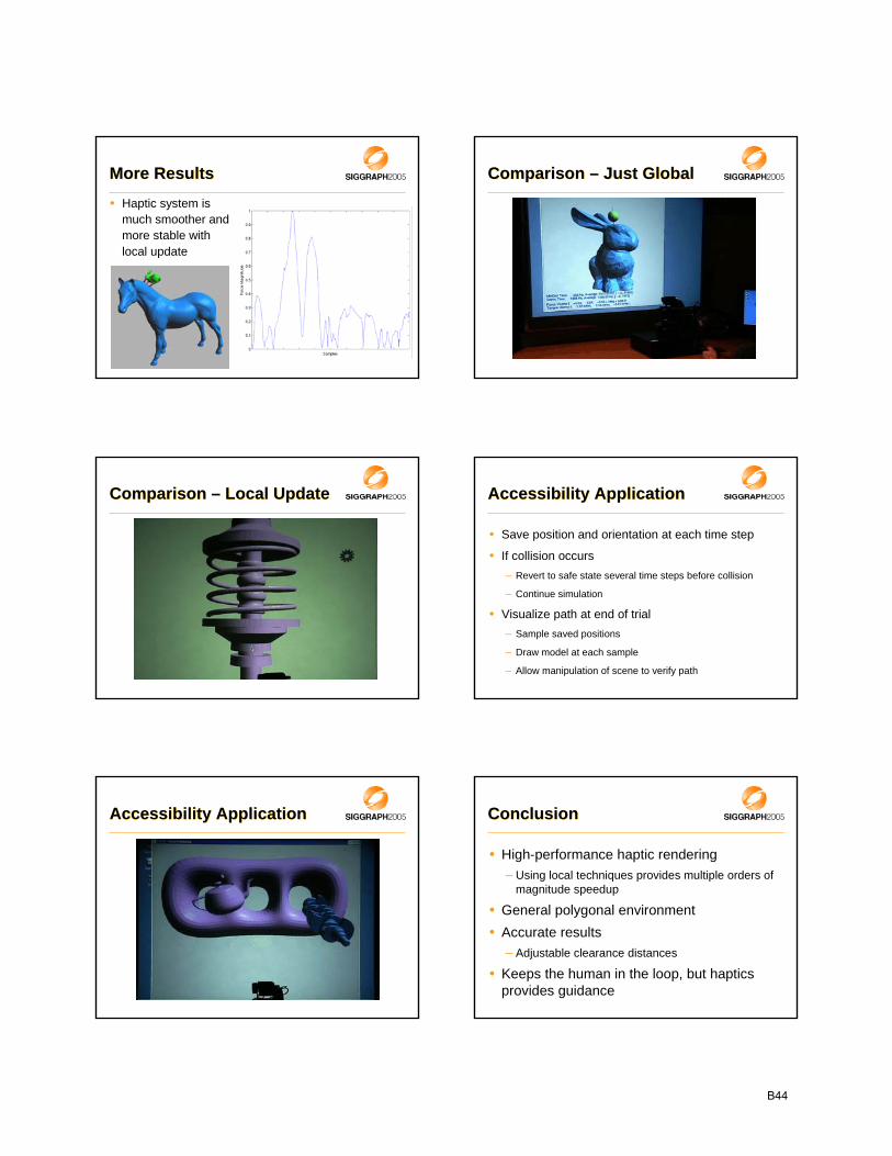
More ResultsMore Results• Haptic system is
much smoother and more stable with local update
Comparison – Just GlobalComparison – Just Global
Comparison – Local UpdateComparison – Local Update Accessibility ApplicationAccessibility Application
• Save position and orientation at each time step
• If collision occurs– Revert to safe state several time steps before collision
– Continue simulation
• Visualize path at end of trial– Sample saved positions
– Draw model at each sample
– Allow manipulation of scene to verify path
Accessibility ApplicationAccessibility Application ConclusionConclusion
• High-performance haptic rendering– Using local techniques provides multiple orders of
magnitude speedup
• General polygonal environment• Accurate results
– Adjustable clearance distances
• Keeps the human in the loop, but haptics provides guidance
B44

Course: Recent Advances in Haptic Rendering and Applications
Session III: Haptic Rendering of Higher-Order Primitives
Haptic Rendering ofSculptured Models
Elaine Cohen*
University of Utah
http://www.cs.utah.edu/~cohen
* Joint work with Tom Thompson, Don Nelson, and David Johnson
Why Sculptured Models?Why Sculptured Models?
• Prevalent format for manufacture and animation
• Compact and exact representation
• Surface normals vary smoothly
Basic Spline BackgroundBasic Spline Background
• Parametric function– Simple example:
interpolating two points10 )1( PttP −+
0P
1P
Basic Spline BackgroundBasic Spline Background
• Parametric function– Simple example:
interpolating two points
– Weighting control points
10 )1( PttP −+
0P
1P
Basic Spline BackgroundBasic Spline Background
• Parametric function– Simple example:
interpolating two points
– Weighting control points
– Basis functions
10 )1( PttP −+
0P
1P
Basic Spline BackgroundBasic Spline Background
• Extends to – higher-degree basis
functions
– piecewise functions
– Higher dimensional domains
B45
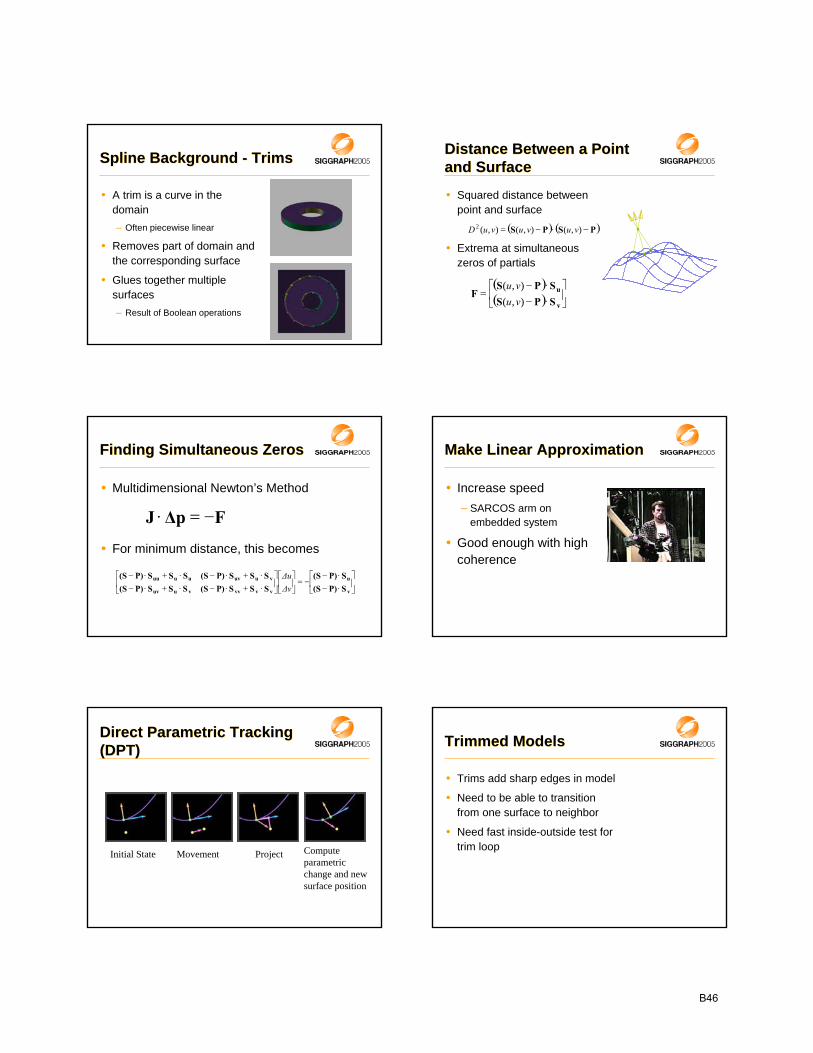
Spline Background - TrimsSpline Background - Trims
• A trim is a curve in the domain– Often piecewise linear
• Removes part of domain and the corresponding surface
• Glues together multiple surfaces– Result of Boolean operations
Distance Between a Point and SurfaceDistance Between a Point and Surface
• Squared distance between point and surface
• Extrema at simultaneous zeros of partials
( ) ( )PSPS −⋅−= ),(),(),(2 vuvuvuD
( )( ) ⎥
⎦
⎤⎢⎣
⎡⋅−⋅−
=v
u
SPSSPS
F),(),(
vuvu
Finding Simultaneous ZerosFinding Simultaneous Zeros
• Multidimensional Newton’s Method
• For minimum distance, this becomes
F∆pJ −=⋅
⎥⎦
⎤⎢⎣
⎡⋅−⋅−
−=⎥⎦
⎤⎢⎣
⎡⎥⎦
⎤⎢⎣
⎡⋅+⋅−⋅+⋅−⋅+⋅−⋅+⋅−
v
u
vvvvvuuv
vuuvuuuu
SP)(SSP)(S
SSSP)(SSSSP)(SSSSP)(SSSSP)(S
∆v∆u
Make Linear ApproximationMake Linear Approximation
• Increase speed– SARCOS arm on
embedded system
• Good enough with high coherence
Direct Parametric Tracking (DPT)Direct Parametric Tracking (DPT)
Initial State Movement Project Compute parametric change and new surface position
Trimmed ModelsTrimmed Models
• Trims add sharp edges in model
• Need to be able to transition from one surface to neighbor
• Need fast inside-outside test for trim loop
B46

Transitioning
• State change while tracing
• Three forms– Across surface boundary
– Along surface intersection
– Off of the model
Edge Tracing and Release
• Slide along trim in 3D to locally close point– Project probe onto current segment– If past endpoint slide– Continue in one direction until minimum reached
• Check for release onto surface– Evaluate surface and apply DPT– If point doesn’t release try adjacent surface
– If point still doesn’t release make special normal
Trim Intersection
• Discrete movement on surface
• Brute force approach not feasible
• Grid approach– Boundary on bounding box
– Locality
– Walk algorithm
Grid Data• Goblet
– 3 surfaces– 254 segs– 13 max– 3 mean– 89% empty
• Gear• 22 surfaces• 1256 segs
• 15 max• 4 mean• 92% empty
• Crank Shaft• 73 surfaces• 412 segs
• 36 max• 4 mean• 89% empty
ExampleExample Example2Example2
B47

Model-model renderingModel-model rendering
• Maintain penetration between two models
• Use Newton’s method to initialize, then integrate to maintain
Differential Surface KinematicsDifferential Surface Kinematics
• Using relations from differential geometry and robotics calibration, the general result for the relation between parametric contact coordinate velocity and body velocity is derived:
Just integrate:
Provides closed form local collision local collision detectiondetection updates.
Surface-to-Surface TracingSurface-to-Surface Tracing
Three step tracking process
Surface-to-Surface ManagementSurface-to-Surface Management
Surface ContactsSurface Contacts
• Possible multiple contacts– Initializing method must
track potential contacts
ExampleExample
• Newton’s method initializes closest points
• Near contact, stable integration takes over
• Maximum penetration is maintained
B48

Course: Recent Advances in Haptic Rendering and Applications
Session IV: Rendering of Textures and Deformable Surfaces
Wearable Vibrotactile Displays
Hong Z. TanHaptic Interface Research Laboratory
Purdue University
http://www.ece.purdue.edu/~hongtan
A Living Proof that Haptics Works! A Living Proof that Haptics Works!
Tadoma
Photograph by Hansi Durlach, 1980.
Sensory Substitution:Text to VibrationSensory Substitution:Text to VibrationOptacon Optohapt
Photograph Courtesy of Telesensory Corp.
Geldard, F. A. (1966). Cutaneous coding of optical signals: The optohapt. Perception & Psychophysics, 1, 377-381.
Sensory Substitution:Image to VibrationSensory Substitution:Image to Vibration
TVSS
White, B. W., Saunders, F. A., Scadden, L., Bach-Y-Rita, P., & Collins, C. C. (1970). Seeing with the skin. Perception & Psychophysics, 7(1), 23-27.
Sensory Substitution:Speech to VibrationSensory Substitution:Speech to Vibration“Felix” Tactaid VII
Photograph byAlfred Eisenstaedt,1950.
Weisenberger, J. M., & Percy, M. E. (1994). Use of the Tactaid II and Tactaid VII with children. The Volta Review, 96(5), 41-57.
Considerations for Wearable Vibrotactile DisplaysConsiderations for Wearable Vibrotactile Displays
• Wearability• Body site• Intended User• Training• Sensory adaptation• Integration with visual and auditory displays
• What is the most effective way to communicate via a vibrotactile display?
B49

Haptic Cueing of Visual Spatial AttentionHaptic Cueing of Visual Spatial AttentionCollaborators: Rob Gray, Jay Young
Blank
Frame 2
Blank
Frame 1
H. Z. Tan, R. Gray, J. J. Young, and R. Traylor, “A haptic back display for attentional and directional cueing,” Haptics-e: The Electronic Journal of Haptics Research, 3(1), 2003.
ApplicationsApplications
Situation AwarenessSituation Awareness
Rupert, A. H. (2000, March/April). An instrument solution for reducing spatial disorientation mishaps - A more "natural" approach to maintaining spatial orientation. IEEE Engineering in Medicine and Biology Magazine, 19, 71-80.
Veen, H.-J. v., Spape, M., & Erp, J. v. (2004). Waypoint navigation on land: different ways of coding distance to the next waypoint. Proceedings of EuroHaptics 2004, 160-165.
Military Silent OperationMilitary Silent Operation
Jones, L. A., Nakamura, M., & Lockyer, B. (2004). Development of a tactile vest. Proceedings of HAPTICS '04, 82- 89.
Limitations in Tactile Information ProcessingLimitations in Tactile Information Processing
0
1
2
3
4
5
6
7
1 2 3 4 5 6 7
Number of stimuli
Res
pons
es
Numerosity Judgments
Tactile Change DetectionTactile Change Detection
time
Offset
Onset
B50

ConclusionsConclusions
• Haptics technology has reached a point where wearable vibrotactile displays are possible
• Many challenges remain in developing lightweight and robust actuators
• We’ve yet to develop a tactile vocabulary that match the sensory capability of the body surface
• More basic research is needed to explore the information-processing limitations in using wearable vibrotactile displays
B51

Course: Recent Advances in Haptic Rendering and Applications
Session IV: Rendering of Textures and Deformable Surfaces
Towards Realistic HapticRendering of Surface Texture
Seungmoon Choi and Hong TanHaptic Interface Research Laboratory
Purdue University
http://www.ece.purdue.edu/~hongtan
OutlineOutline
• Introduction– Texture
– Perceived Instability
• Psychophysical Evaluations
• Sources of Perceived Instability
• Conclusions
What is Texture?What is Texture?
• What is texture?– Texture = micro geometry of a surface
– Shape = macro geometry of a surface
• Why study haptic texture rendering?– To enrich the sensory attributes of virtual objects
– To provide well-controlled stimuli for psychophysicalstudies
(L = 2.5 mm A = 50 µm)
Haptic Texture RenderingHaptic Texture Rendering
• How to render texture haptically?– Haptic texture information can be effectively conveyed
through temporal cues alone (e.g., Katz’ observations)
– Point-contact probe-mediated force feedback devices can adequately render virtual textures
• Past work has focused on the developments of fast computational algorithms – Massie (1996) − force magnitude
– Ho et al. (1999) − force magnitude & direction
Perceived InstabilityPerceived Instability
• Definition: Any unrealistic sensation that can not be attributed to the physical properties of simulated textured surfaces (e.g., buzzing).
• Types of Perceived Instability– “Buzzing”
– “Aliveness”
– “Ridge Instability”
• Can be caused by both device instability and inadequate environment model
OutlineOutline
• Introduction– About Texture
– Perceived Instability
• Psychophysical Experiments
• Sources of Perceived Instability
• Conclusions
B52

ApparatusApparatus
• PHANToM 1.0A (SensAble Technologies, MA)
Texture ModelTexture Model
• Free Exploration vs. Stroking
Main FindingsMain Findings
• Largest stiffness values for “clean” texture:0.01 to 0.78 N/mm (“soft corduroy”)
• Largest stiffness value for “clean” flat wall:1.005 N/mm
• We need a better understanding of the types of perceived instabilities and their underlying causes
• The goal is to be able to render “harder” textures without any perceived instability
Three Types ofPerceived InstabilitiesThree Types ofPerceived Instabilities
• Buzzing– Perceived as high-frequency noises (“vibrating” textures)
• Aliveness– Perceived as low-frequency force variations (“pulsating”
textures) when the stylus is stationary
• Ridge Instability– When resting on the peak of a sinusoidal ridge, the stylus
is being pushed into the valley.
OutlineOutline
• Introduction– About Texture
– Perceived Instability
• Psychophysical Experiments
• Sources of Perceived Instability
• Conclusions
BuzzingBuzzing
|Pz(f)|: dB re 1µm peak, Perceived Magnitude: dB SL
B53

What Causes Buzzing?What Causes Buzzing?
Measured at the origin of the PHANToM with the stylus pointing to the +z direction
PHANToM Frequency Response
AlivenessAliveness
Signal duration = 400 ms
What Causes Aliveness?What Causes Aliveness?
• Our hypothesis was that Aliveness came from the texture rendering algorithm, but not an unstable haptic interface
• To test our hypothesis, we implemented a Passivity Observer (Hannaford & Ryu, 2002) on measured force and position data
Passivity ObserverPassivity Observer
Passive Rendering with AlivenessPassive Rendering with Aliveness
px(t): mm, pz(t): mm, FzW(t): N, PO (t): Nmm/sec
What Causes Ridge Instability?What Causes Ridge Instability?
B54

ConclusionsConclusions
• Many virtual textures contain perceived instability• Stroking is the preferred method for texture
perception because it has a larger stiffness threshold for perceived instability
• Perceived instability can occur even when the haptic interface system is passive
• Research based on both control and perception are necessary in order to achieve perceptually realistic texture rendering
B55

Course: Recent Advances in Haptic Rendering and Applications
Session IV: Rendering of Textures and Deformable Surfaces
Haptic Rendering ofTextured Surfaces
Miguel A. Otaduy
ETH-Zurich
http://graphics.ethz.ch/~otmiguel
OutlineOutline
• Motivation
• Algorithm Overview
• Synthesis of the Force Model
• Penetration Depth on the GPU
• Experiments and Results
• Conclusion
IntroductionIntroduction IntroductionIntroduction
• Geometric surface texture:– Compelling cue to object identity
– Strongly influences forces during manipulation
• Objects with rich surface texture information cannot be handled by state-of-the-art hapticrendering methods.
ModelsModels
Coarse geometric representations
Haptictextures
OutlineOutline
• Motivation
• Algorithm Overview
• Synthesis of the Force Model
• Penetration Depth on the GPU
• Experiments and Results
• Conclusion
B56

simplified surface
contact pointheight field in texture map
3-DoF Texture Rendering3-DoF Texture Rendering
• 1 contact point on a textured surface– Minsky [1995], Ho et al. [1999]: high frequency
forces based on gradient of height field
3-DoF Texture Rendering3-DoF Texture Rendering
• 1 contact point on a textured surface– Siira and Pai [1996]: stochastic model
– Pai et al. [2001]: auto-regressive model for roughness and friction
6-DoF Texture Rendering6-DoF Texture Rendering
• Object-object interaction– Contact cannot be described as point-surface
contact
– Force and torque output has 6-DoF; point contact only has 3-DoF
• A different rendering algorithm is required
Rendering AlgorithmRendering Algorithm
1) Compute contact information betweenlow-res models
Rendering AlgorithmRendering Algorithm
1) Compute contact information betweenlow-res models
2) Refine contact information using detail geometry stored in textures
Rendering AlgorithmRendering Algorithm
1) Compute contact information betweenlow-res models
2) Refine contact information using detail geometry stored in textures
3) Compute contact forces based on novel texture force model
B57

Force Model OverviewForce Model Overview
• Accounts for important factors identified by perceptual studies
• Based on the gradient of inter-object penetration depth
• GPU-based computation of directional penetration depth
OutlineOutline
• Motivation
• Algorithm Overview
• Synthesis of the Force Model
• Penetration Depth on the GPU
• Experiments and Results
• Conclusion
Related Work:Perception & Psychophysics
Related Work:Perception & Psychophysics
• Studies on perception of textures through a rigid probe by Klatzky and Lederman [1999-present]– Analyze effects of probe diameter, applied force
and exploratory speed
– Inspiration for our force model
log (texture frequency)
log
(rou
ghne
ss)
Probe Diameter (D)Applied Force (F)Exploratory Speed (v)
Roughness Vs. Texture Spacing[Klatzky and Lederman 1999-present]
Roughness Vs. Texture Spacing[Klatzky and Lederman 1999-present]
log (texture frequency)
log
(rou
ghne
ss)
D+
- Strong influence of geometry
Effect of Probe Diameter (D)[Klatzky and Lederman 1999-present]
Effect of Probe Diameter (D)[Klatzky and Lederman 1999-present]
log (texture frequency)
log
(rou
ghne
ss)
F+
-
Roughness grows with applied force
Effect of Applied Force (F)[Klatzky and Lederman 1999-present]
Effect of Applied Force (F)[Klatzky and Lederman 1999-present]
B58

log (texture frequency)
log
(rou
ghne
ss)
v+
-
Dynamic effects already present in haptic simulation
Effect of Exploratory Speed (v)[Klatzky and Lederman 1999-present]
Effect of Exploratory Speed (v)[Klatzky and Lederman 1999-present]
Use offset surface as descriptor of vibration
How can we generalize offset surfaces?
Offset SurfacesOffset Surfaces
Spherical probe trajectory = offset surface
Arbitrary objects ???
δ
Penetration Depth: DefinitionPenetration Depth: Definition
= Minimum translational distance to separate two intersecting objects
δ
= Minimum translational distance to separate two intersecting objects
Penetration Depth: DefinitionPenetration Depth: Definition
δ
= Minimum translation along n to separate two intersecting objectsnδ
n
Directional PD: DefinitionDirectional PD: Definition
= Minimum translation along n to separate two intersecting objects
n
nδ
Directional PD: DefinitionDirectional PD: Definition
nδ
B59

Textured surface
Offset surface
Offset Surface and PDOffset Surface and PD Offset Surface and PDOffset Surface and PD
Textured surface
Offset surface
δ
h
h=δ≡δ penetration depth
Offset Surface and PDOffset Surface and PD
2
21 δkU =
Force ModelForce Model
• Penetration depth:– Applicable to arbitrary object-object interaction
– Also used in previous single-point rendering methods
• Penalty-based potential field:
( ) ( )
⎟⎟⎠
⎞⎜⎜⎝
⎛∂∂
∂∂
∂∂
∂∂
∂∂
−
=∇−=−∇=
n
n
v
n
u
nnnn
nnnvunvu
vuk
kUTTTFFF
θδ
θδ
θδδδδ
δδ
1
Force ModelForce Model
• Determine penetration direction n
• Force and Torque = Gradient of energy:
• Force and torque proportional to gradient of penetration depth
High amplitude texture
High derivative of penetration depth
Large force/torque
Method validated by Minsky [1995]
( ) ( )nnnvunvu kTTTFFF δδ ∇−=
Effect of GeometryEffect of Geometry
B60

• Normal force:
• Other forces and torques:
Larger normal force Larger roughness effect
nn kF δ−=
uF
ukF n
nn
nu ∂∂
=∂∂
−=δδδ
Effect of Applied ForceEffect of Applied Force OutlineOutline
• Motivation
• Algorithm Overview
• Synthesis of the Force Model
• Penetration Depth on the GPU
• Experiments and Results
• Conclusion
= Minimum translation along n to separate two intersecting objects
n
nδ
Directional PD: DefinitionDirectional PD: Definition
nδ ( )BAn hh −= maxδ
nBA hh −
B
A
Directional PD of Height FieldsDirectional PD of Height Fields
PD with Texture ImagesPD with Texture Images
n
Low-res Surface
High-resSurface
PD with Texture ImagesPD with Texture Images
n
Low-res Surface
High-resSurface
B61

PD with Texture ImagesPD with Texture Images
n
Low-res Surface
High-resSurface
PD with Texture ImagesPD with Texture Images
n
Low-res Surface
High-resSurface
PD Computation AlgorithmPD Computation Algorithm Low-Resolution Models…Low-Resolution Models…
…+ Texture Images…+ Texture Images Step 1: Approximate PDStep 1: Approximate PD
B62

Step 1: Approximate PDStep 1: Approximate PD Step 2: Refined PDStep 2: Refined PD
Pass 1: Render GeometryPass 1: Render Geometry Pass 1: Texture MappingPass 1: Texture Mapping
Pass 1: Sample SurfacesPass 1: Sample Surfaces Pass 1: Project to PD DirectionPass 1: Project to PD Direction
B63

Discrete Height Fields Discrete Height Fields Pass 2: Subtract Height FieldsPass 2: Subtract Height Fields
Pass 2: Copy to Depth BufferPass 2: Copy to Depth Buffer Binary Search for Max = PD[Govindaraju et al. 2004]
Binary Search for Max = PD[Govindaraju et al. 2004]
TestTest TestTest
B64

( ) ( )
⎟⎟⎠
⎞⎜⎜⎝
⎛∂∂
∂∂
∂∂
∂∂
∂∂
−
=∇−=−∇=
n
n
v
n
u
nnnn
nnnvunvu
vuk
kUTTTFFF
θδ
θδ
θδδδδ
δδ
1
Gradient of PDGradient of PD
• Central differences
• Recompute PD at 2 new object configurations
( ) ( )u
nvuunvuuu
nnn
∆⋅∆−−∆+
≈∂∂
2,...,,,...,, δδδ
Gradient of PDGradient of PD
OutlineOutline
• Motivation
• Algorithm Overview
• Synthesis of the Force Model
• Penetration Depth on the GPU
• Experiments and Results
• Conclusion
ExperimentsExperiments
• Offline analysis of force model
• Quality of texture effects
• Performance tests.
Offline ExperimentsOffline Experiments
δn
bh
kh
mh
vDn
u
0.8 1 2 4 61
2
5
10
20
50
Texture Spacing (mm)
Max
imum
Acc
eler
atio
n
1mm2mm3mm
Studies by Klatzky and Lederman Simulation results
Effect of Probe DiameterEffect of Probe Diameter
B65
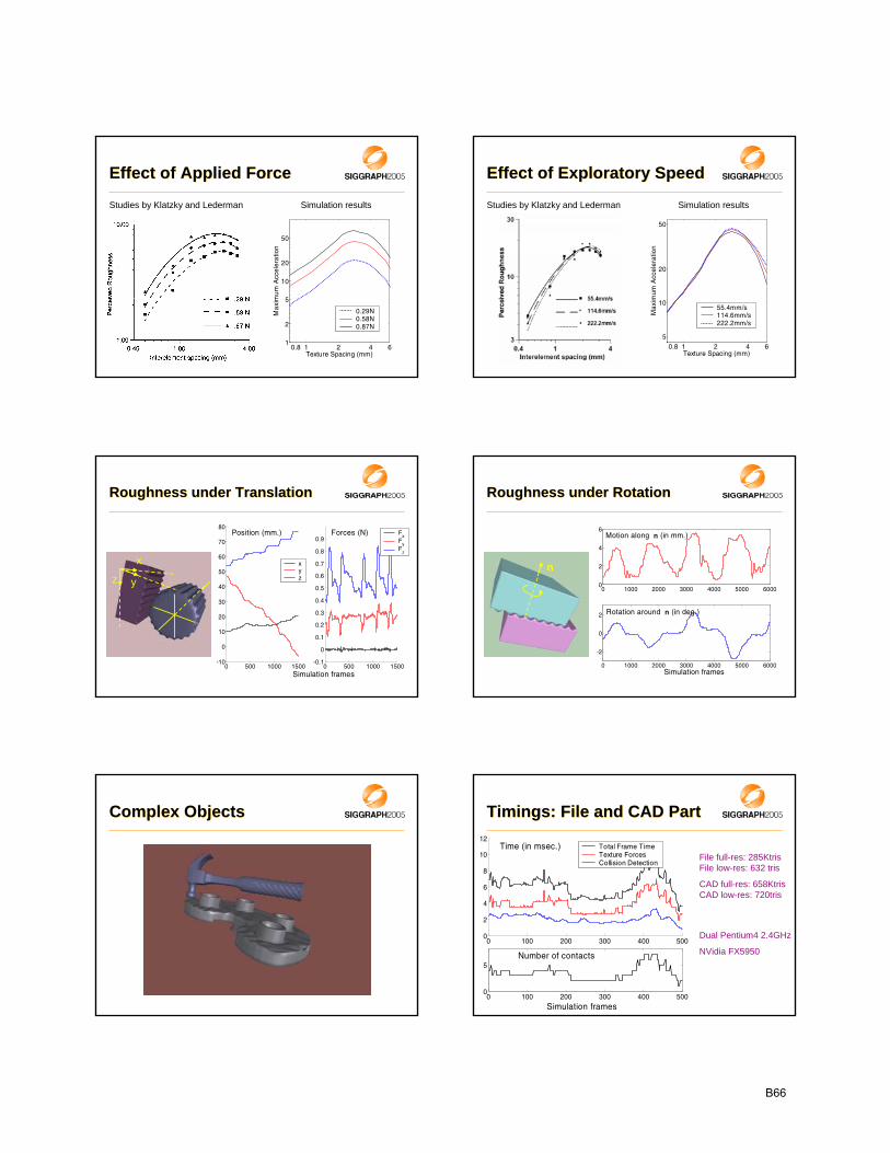
Effect of Applied ForceEffect of Applied Force
0.8 1 2 4 61
2
5
10
20
50
Texture Spacing (mm)
Max
imum
Acc
eler
atio
n
0.29N0.58N0.87N
Studies by Klatzky and Lederman Simulation results
Effect of Exploratory SpeedEffect of Exploratory Speed
0.8 1 2 4 65
10
20
50
Texture Spacing (mm)
Max
imum
Acc
eler
atio
n
55.4mm/s114.6mm/s222.2mm/s
Studies by Klatzky and Lederman Simulation results
0 500 1000 1500-10
0
10
20
30
40
50
60
70
80
0 500 1000 1500-0.1
0
0.1
0.2
0.3
0.4
0.5
0.6
0.7
0.8
0.9
xyz
Fx
Fy
Fz
Position (mm.) Forces (N)
Simulation frames
z y
x
Roughness under TranslationRoughness under Translation
0 1000 2000 3000 4000 5000 60000
2
4
6
0 1000 2000 3000 4000 5000 6000
-2
0
2
Motion along n (in mm.)
Rotation around n (in deg.)
Simulation frames
n
Roughness under RotationRoughness under Rotation
Complex ObjectsComplex Objects
0 100 200 300 400 5000
2
4
6
8
10
12
0 100 200 300 400 5000
5
Total Frame TimeTexture ForcesCollision Detection
Time (in msec.)
Number of contacts
Simulation frames
File full-res: 285KtrisFile low-res: 632 tris
CAD full-res: 658KtrisCAD low-res: 720tris
Dual Pentium4 2.4GHz
NVidia FX5950
Timings: File and CAD PartTimings: File and CAD Part
B66

OutlineOutline
• Motivation
• Algorithm Overview
• Synthesis of the Force Model
• Penetration Depth on the GPU
• Experiments and Results
• Conclusion
SummarySummary
• Haptic rendering algorithm usinglow-res models and texture images
• Force model inspired by psychophysics studies
• Image-space algorithm for PD computation (implemented on GPU)
ResultsResults
• 500Hz force update rate with relatively simple models
• 100Hz-200Hz force update rate with complex models
• Haptic rendering of interaction between complex textured models
LimitationsLimitations
• Cannot handle surfaces that cannot be described as height fields in the contact region
• Possible sampling-related aliasing
• Limited stability with high PD gradient
Future WorkFuture Work
• Higher frequency textures
• Deformable textured surfaces
• Analysis of human factors
ReferencesReferences
Haptic Display of Interaction between Textured Models.Miguel A. Otaduy, Nitin Jain, Avneesh Sud and Ming C. Lin.In Proc. of IEEE Visualization Conference 2004.
A Perceptually-Inspired Force Model for Haptic Texture Rendering. Miguel A. Otaduy and Ming C. Lin.In Proc. of the Symposium on Applied Perception in Graphics and Visualization 2004.
http://gamma.cs.unc.edu/HTextures/
B67

1
Modeling Deformable Objects for Haptics
Modeling Deformable Objects for Haptics
Dinesh K. Pai
(mostly in collaboration with Doug James)
Rutgers University
OutlineOutline
• Basics of Elasticity
• Linear Elastostatic Models
• Green’s Functions
• Capacitance Matrix Algorithms
• Haptic Interaction Issues
• Extensions
[James + Pai 99]
Interactive DeformationInteractive Deformation
ElasticityElasticity
• Dynamics defined at infinitesimal scale– force -> stress
– displacement -> strain
– Hooke’s law relates stress to strain
– Newton -> Cauchy
• Hyperbolic partial differential equations
• PDE + boundary conditions = Boundary Value Problem (BVP)
Linear Elastostatic ModelsLinear Elastostatic Models
• Simple but stable
• Captures many “global” aspects of deformation
• Sufficient to only deal with boundary discretization
• Significant precomputation
• But inaccurate for some materials, large deformation
n = 0.5
021
13
1
2
2
2
=+⎟⎟⎠
⎞⎜⎜⎝
⎛∂∂
∂−
+∂∂∑
=i
k ik
k
k
i bxx
uxuG
ν
Numerical DiscretizationNumerical Discretization
• Most problems must be solved numerically– Finite Differences
– Finite Element Method (FEM)
– Boundary Element Method (BEM)
• FEM => internal discretization; easy to handle anisotropy and inhomogeniety
• BEM=> only boundary discretization; easy to handle mixed boundary conditions
B68

2
Key Idea: Green’s FunctionsKey Idea: Green’s Functions
u = U p
=
Green’s Functions
j
pj
j
j
Green’s functions U relateu, vertex displacements to
p, applied vertex tractions
Can be computed analytically ifmaterial distribution is known
Related work:
Cotin et al. 96 “Condensation”
Astley & Hayward 98 “Norton equivalents”
James and Pai 99 “Green’s functions” via BEM
Example: Boundary Elements Example: Boundary Elements
∫∫ΓΓ
Γ=Γ+ dd p*u u*puc
H u = G pH u = G p
Constant Elements
PointLoadat j
i
gij
Weaken,Integrate
021
13
1
2
2
2
=+⎟⎟⎠
⎞⎜⎜⎝
⎛∂∂
∂−
+∂∂∑
=i
k ik
k
k
i bxx
uxuG
ν
N u + b = 0
Discretize
Green’s Functions for Discrete BVP (via BEM)
H u = G p
SPECIFY BC
RedRed BV specifiedBV specifiedYellowYellow BV unknownBV unknown
REARRANGE
A v = - A v_ _
=
=
=
=
INVERT LHS
v = - A-1 A v = Ξ v_ _ _
Green’s Functions
• Usually few specified BV’s are nonzero
• If s (out of n) non-zero BVs,O(ns) time to evaluate
Fast Solution to BVP with Green’s FunctionsFast Solution to BVP with Green’s Functions
v = Ξ v_
• Problem:
– if BC changes, have to recompute Ξ
–Ξ large and dense
Boundary Condition Type ChangesBoundary Condition Type Changes
• Idea: Exploit coherence
Fast ElastostaticDeformationFast ElastostaticDeformation
• BC change swaps a block column of A
= H u = G p
= +
Ts
0s E A A A δ+=
vA- v A ss =
B69

3
Notation Notation
• E is n x s submatrix of IdentityM E “Extracts” columns from matrix MNo cost
• Change in matrix
• Changed columns)EAA( A
0 0 −=sδ
T 0
0
0s )EEAA( A A −+=
Ts
0s E A A A δ+= = +
Sherman-Morrison-WoodburySherman-Morrison-Woodbury
• Idea: Exploit coherence between BVPs
[ ] 1-0
Ts
1-0
Ts
1-0
1-0
1-s AEA AEI A A- AA 1−
+= δδ
Ts
0s E A A A δ+=• If• If = +
s-by-s capacitance matrix (small)s-by-s capacitance matrix (small)
• Exploit coherence using SMW formula
• When s nodes switch, extract and factorC = -ETΞE = s-by-s capacitance matrix
Capacitance Matrix Algorithm [James + Pai 99,01]
Capacitance Matrix Algorithm [James + Pai 99,01]
_–Henceforth, v(0) = [ Ξ(I-EET) - EET ] v
v = v(0) + (I+Ξ)EC-1ET v(0)
E “extracts” the s columns
O(s3) or better
O(n s)
• video
[James, Pai SIGGRAPH 99]
Haptic Interaction [James & Pai 01]Haptic Interaction [James & Pai 01]
• Need to update contact force at much higher rate (1 KHz)– Idea: use faster local model at contact point
– Related work: [Astley & Hayward 98], [Balanuik00], [Cavsolglu & Tendick 00]
• Need to support “point contact” abstraction (e.g., for PHANToM)
Local Models from the Capacitance Matrix AlgorithmLocal Models from the Capacitance Matrix Algorithm• Region of Interest
– If output is needed only at d nodes (with extraction matrix ED),
EDT v = ED
T v(0) + (EDT(I+Ξ)E)C-1ET v(0)
in O(d s + s 2) time
_
• If these are the same s contacting nodes, simplifies dramatically!
ET v = -C-1ET v⇒ an exact “local buffer” for haptics
B70

4
Point Contact abstractionPoint Contact abstraction
• Real point contact produces infinite tractions (and therefore larger displacements on finer mesh)
• Use vertex masks to distribute displacement over finite area [James & Pai 01]
Capacitance Matrix in Haptics
Multiresolution Green’s FunctionsMultiresolution Green’s Functions
[James and Pai 02]
DyRT [James & Pai 02]DyRT [James & Pai 02]
Dynamicphysically-based modal deformation
Responseto bone-based animation
Texturesprecomputed, sampled, and rendered
almost entirely on graphics hardware
Dynamicphysically-based modal deformation
Responseto bone-based animation
Texturesprecomputed, sampled, and rendered
almost entirely on graphics hardware
DyRT movieDyRT movie
Surgical Simulation
[James & Pai 02]
B71

5
ResourcesResources
• Gibson and Mirtich “A Survey of Deformable Models in Computer Graphics” MERL Tech Report TR-97-19, 1997
– www.merl.com
• James & Pai SIGGRAPH 99 contains a review of elastic models
– www.cs.ubc.ca/~pai/papers/JamPai99.pdf
• James & Pai “A Unified Treatment of Elastostatic and Rigid Contact Simulation for Real Time Haptics”, to appear (2001) in Haptics-e The Electronic Journal of HapticsResearch
– www.haptics-e.org
ExtensionsExtensions
Thin strandsThin strands
• E.g., surgical sutures (“threads”), hair, etc.
• Cosserat model may be more efficient [Pai, Eurographics 02]
+ reduces to a 1D problem
+ handles geometric non-linearities
+ fast (similar to rigid body chain)
- useful for thin objects only
Simulator
Exploiting reduced coordinates for collision detectionExploiting reduced coordinates for collision detection
Traditional collision detectors don’t care about reduced coordinates
...
q
Collision Detector
. . :
Simulator
BD-Tree [James&Pai SIGGRAPH 04]BD-Tree [James&Pai SIGGRAPH 04]
q
BD-Tree
. . .
qq q
q
Bounded Deformation tree
Idea: Parameterize bounding volumes by reduced coordinates
Fast Sphere UpdateFast Sphere Update
• Storage cost: 4 floats / mode
• Amortized cost: 8 flops / mode
• Spheres can be updated in any order
and without access to geometry
Output-sensitive collision detection
B72

6
Reality-based Modeling for Haptics and Multimodal DisplaysReality-based Modeling for Haptics and Multimodal Displays
Dinesh K. Pai
Rutgers University
Multisensory integration can improve haptic perceptionMultisensory integration can improve haptic perception
e.g., [Doel, Kry and Pai, SIGGRAPH 01]
Integrating Audio Haptic DisplaysIntegrating Audio Haptic Displays
User InteractionUser Interaction
• Contacts are rendered atomically, with haptics andsound
• Same contact forces drive both haptics and sound
• Haptic force and sound synchronized to < 1ms
• Using
– Sound synthesis algorithm of [van den Doel & Pai]
– Pantograph haptic device of [Hayward & Ramstein]
– Custom DSP controller
[DiFilippo and Pai UIST 00]
The AHI Audio-HapticInterfaceThe AHI Audio-HapticInterface
DiFilippo and Pai UIST 00
ResultsResults
Force
B73

7
How to get models for contact simulation?How to get models for contact simulation?
• Haptic interaction and, more generally, contact requires multisensory models
• Need parametrized models that support low-latency multisensory interaction
• Need to measure geometry, elastic deformation, sound response, friction, roughness, etc.
Reality-based modelingof Contact
Reality-based modelingof Contact
[Pai, van den Doel, James, Lang, Lloyd, Richmond, Yau
SIGGRAPH 2001]
Our Focus: Scanning Contact Interaction BehaviorOur Focus: Scanning Contact Interaction Behavior
OverviewOverview
• ACME, a robotic facility for scanning contact behavior
• Scanning contact deformation models
contact sound models
contact texture models
ACMEThe UBC Active Measurement Facility
ACMEThe UBC Active Measurement Facility
[Pai,Lang,Lloyd,Woodham ‘99]
B74

8
Preview: Scanning Contact FrictionPreview: Scanning Contact Friction
Video
A Framework for ScanningReality-based ModelsA Framework for ScanningReality-based Models
Model Structure
Measurement
Estimation
Rendering
Scanning Deformation BehaviorScanning Deformation Behavior
Model Structure: Green’s FunctionsModel Structure: Green’s Functions
• u = Up• =
Green’s Functions
Linear Elastostatic Model+Reference boundary conditions
Green’s functions U relateu, vertex displacements to
p, applied vertex tractions
Can be computed analytically if material distribution is known
e.g., [JamesPai99, Cotin et al 96,...]
Model Structure: Green’s FunctionsModel Structure: Green’s Functions
• u = Up• =
Green’s Functions
j
pj
j
j
Linear Elastostatic Model+Reference boundary conditions
Green’s functions U relateu, vertex displacements to
p, applied vertex tractions
Can be computed analytically ifmaterial distribution is known
e.g., [JamesPai99, Cotin et al 96,...]
MeasurementMeasurement
Robot arm measures contact force and local displacement
Global displacement measured with stereo vision and range flow Details in [LangPai01]
B75

9
Parameter EstimationParameter Estimation•Excite vertex j with several pj
k
estimate vertex displacement uik from range flow
Parameter EstimationParameter Estimation
•Interpolate missing observations
•Estimate Uij robustlyusing TSVD, TLS
Results Results
Interactive Rendering DemoInteractive Rendering Demo
Rendered using capacitance matrix algorithmwith haptic force computation at 1KHz [JamesPai99, JamesPai01]
B76

10
Scanning Contact TextureScanning Contact Texture
What is Contact Texture?What is Contact Texture?
• Physical parameters relevant to human perception of contact [Lederman Klatzky ... ]
• Texture = friction + roughness + …
• Model should support fast simulation for haptics (1 KHz) and audio (44.1 KHz)
Measurement:Measurement:•Easy for small sample
•Hard for general object: uncertainty in surface normal, adaptation
•We use differential measurementtechnique for robust estimation
FrictionFriction
• Estimate: normal and friction together
• Model: Coulomb Friction ft = -µ | fn | u
RoughnessRoughness
• Traditionally ≈ small scale variation in surface geometry
• Our model: small scale variation in friction– Equivalent to traditional model, for frictional contact
– Unifies friction and roughness haptic rendering
Example: Clay PotExample: Clay Pot
Fn
Ft
µ
RoughnessRoughness• Model structure: AR(p) autoregressive model
– Captures randomness plus periodicities
– Small p sufficient for many surfaces [Thomas 82, Perlin]
• Estimate parameters: using covariance method
• Rendering: Discrete convolution
• Extremely fast and simple
)(~)( xxe µµµ +=
kik
p
iik a σεµµ += −
=∑ ~~
1
B77

11
Real vs. Simulated Clay PotReal vs. Simulated Clay Pot
Real µ
Sim µ
Scanning the Clay PotScanning the Clay Pot
Scanning Contact SoundsScanning Contact Sounds
Contact SoundsContact Sounds
• Provide cues of contact shape, location, force, and object material
• “Foley sounds” in radio and cinema
• Can be integrated with – Simulation and Interaction
[O’BrienCookEssl, DoelKryPai, Friday]
– Room acoustics [e.g., Tsingos et al., Friday]
Model StructureModel Structure
• Modal Synthesis [e.g., Doel&Pai 96-01, Cook 96]
• Models impulse response at surface point
•fi is frequency of a vibration modedi is frequency-dependent damping
• ai(x) location dependent amplitude “texture”
• Continuous contact sounds generated by convolution with contact force
( ) ∑=
−=M
ii
tdi tfexatxp i
1
)2sin()(, π ++
+
Measure Impulse ResponseMeasure Impulse Response
B78

12
Estimate ParametersEstimate Parameters
Refine frequencies + estimate aik , di[SteiglitzMcBride65, BrownPuckette93]
First estimate modal frequencies fi
original
10 modes
90 modes
30 modes
• Generate contact force at audio rates – depends on contact texture,
nominal force, and velocity [see DoelKryPai paper on Friday]
• Convolve with audio impulse response– efficient using modal resonator filter bank
(4 flops/mode/sample)
– smoothly interpolate audio parameters ai(x) from mesh vertices
RenderingRendering
Scanning the Clay PotScanning the Clay Pot
Video
ConclusionsConclusions
• It is now possible to scan multi-modal models of contact interaction behavior
• Scannable behavior includes– deformation (visual and haptic)– friction and roughness texture– sound response
• Can be automated with ACME, a robotic measurement facility
B79

Course: Recent Advances in Haptic Rendering and Applications
Session V: Novel Applications
Applications inScientific Visualization
Russell Taylor
UNC-Chapel Hill
http://www.cs.unc.edu/~taylorr
Outline of Taylor talkOutline of Taylor talk
• Eight scientific haptic applications
• Three haptic applications in more depth– Listing benefits found from haptics in each
– Showing mechanism for coupling haptics thread
• (Brief) Haptics for multivariate display
Molecular Dynamics Application
Molecular Dynamics Application
• VMD: Visual Molecular Dynamics
Humphrey, 1996
Haptic Vector FieldApplication
Haptic Vector FieldApplication
• Lawrence, Lee, Pau, Roman, Novoselov– University of Colorado at Boulder
• 5 D.O.F. in
• 5 D.O.F. out
Lawrence, 2000
Volume Flow VisualizationUser Study
Volume Flow VisualizationUser Study
• Iwata and Noma combined HMD and haptics to display volume data in 1993– Force based on density gradient
– or Torque based on density
– Either method improved positional accuracy
• Describe presenting flow field– Force for flow velocity
– Torque for vorticityIwata, 1993
B80

Medical Volume ExplorationApplication
Medical Volume ExplorationApplication
• Avila and Sobierajski 1996– Feeling neuron dendrites
• Repulsion was too hard to follow for twisting dendrites
– Gentle attraction used• Opposite of gradient
Avila, 1996
Vector and Tensor Field Applications
Vector and Tensor Field Applications
• The Visual Haptic Workbench
Constrain to streamline Anisotropic drag
Ikits, 2005
• Teaching physics potential fields
• Drug/protein docking• nanoManipulator
When is Force Useful?UNC Experiences
When is Force Useful?UNC Experiences
Force-Field Simulation for Training
Force-Field Simulation for Training
• 2D sliding carriage device
• Presented magnetic, electric, and gravitational fields
• Motivated students learned more
– Less motivated students didn’t
• Dispelled misconceptions
– Electric field in diode is not greater near the plate than near the cathode
– Gravity field in 3-body system does not always point towards one of the bodies
Brooks, 1990
Drug/Protein DockingDrug/Protein Docking
• Ming Ouh-Young– 6-DOF positioning task
– “Lock and Key” problem
– Hard surface + electrostatic
– Got a better “feel” for docking
– User study: NTE factor-of-2 speedup with haptics
Brooks, 1990
B81

A virtual environment interface to SPM
The Goal:• Remove boundaries
between user and sample• Can we make experiments
on the molecular scale aseasy as rolling a pencil orpushing a golf ball?
nanoManipulatornanoManipulator nanoManipulator: HapticsnanoManipulator: Haptics
“It was really a remarkable feeling for a chemist to be running his hand over atoms on a surface”– R. Stanley Williams, UCLA Chemistry
• Exciting and engaging, but what is it useful for?
Finding the right spotFinding the right spot
Positionwhenscanning
Positionafter being heldstill for several seconds
Also, finding the top of an adenovirus
Finding the right pathFinding the right path
Light touch (haptic imaging)Light touch (haptic imaging)
Observation modifies the system
B82

• Problem: Haptics must update at >500 Hz– Required for stable hard surfaces
– Must be uninterrupted to prevent force discontinuities
• Solution: As Ken & Ming described– Separate force-feedback server
– Pass Intermediate representation between threads
Case Study ofMulti-ThreadingCase Study of
Multi-Threading nManipulator: The Old Way
Move Microscope Tip, Read HeightSend Force (Depends on Height)
Draw Image
Position
Force
Force-FeedbackDevice
Video
User Interface controls force and
microscope
Server measures end effectorlocation
11 User interface moves microscope tip to track end effector motion
22
Two samples + “up” yield a tangent plane to the surface at contact point
33Plane is transformed into device coordinates and presented to user
44
Phantom
SPM
Decoupling surface update using intermediate rep.
Decoupling surface update using intermediate rep.
ProbeLocal Plane
Approximation(Used in Force Loop)
Surface
Complete Surface(known to
Application)
Local Plane EquationLocal Plane Equation
• Discontinuity when plane updated
Probe
t = 0 t > 0Probe is beneaththe updated plane
Result: Large force
Preventing DiscontinuityPreventing Discontinuity
Probe
t = 0 t > 0Probe is broughtgradually toupdated plane
• Recovery time over several steps
10ms update enabled10X stable stiffness
Preventing DiscontinuityPreventing Discontinuity
B83

SEM+AFM: See while touchSEM+AFM: See while touch
• SEM view of AFM tip
• Hand-controlled AFM
• Zooms in on nanotube
• “Twangs” nanotube
3D Magnetic Force Microscope
3D Magnetic Force Microscope
Sandpaper: Haptic TexturesSandpaper: Haptic Textures
• Margaret Minsky dissertation (MIT, UNC)• Displayed 3D surfaces on 2D haptic device by
mapping slope to lateral force– People perceived 3D shape
• Displayed several properties– Viscosity
– Spatial Frequency
• Vary properties based on data
Minsky, 2000
Augmenting “Basic Haptics”Augmenting “Basic Haptics”
• Jason Fritz, University of Delaware– Adding haptic “grid planes” provide scale
– Friction and texture• Produce more realistic-feeling surfaces
• Can distinguish features in data sets
– Produced stochastic texture model• Creates information-rich haptic textures
Fritz, 1996
B84

Haptics for Multi-Dimensional Display
Haptics for Multi-Dimensional Display
• Modulate surface properties– friction, stiffness, bumpiness, vibration, adhesion
• User studies done by Mark Hollins at UNC to determine the perceptually-linear mapping for each– Map directly for the relevant physical parameter
– Linearize for presentation of non-physical quantities
• Ongoing exploration of cross-talk between channels
Seeger, 2000
SummarySummary
• Useful for– Direct perception of force fields
– Sensing while manipulating simulation or tele-operation
– Tracing without occlusion in 3D
• Match application requirements– 2DOF in/out for force fields
– 6DOF in/out for Docker
– 6DOF in, 3DOF out for nM
• Separate force, graphics and control loops
nanoManipulator Co-builders(78)
nanoManipulator Co-builders(78)
Belgium
Toronto
ASU
WPAFB
NIST
Information & Library Science
Education CS Dist. Sys.
Gene Therapy
PhysicsCS Graphics
CS Image Biology
Chemistry
NIEHSRTP
Psychology
3rdTech
Support provided bySupport provided by
– 3DMFM• NIH National Institute for Biomedical Imaging and
Bioengineering
• NIH National Center for Research Resources
• National Science Foundation
• Army Research Office
• Office of Naval Research
ReferencesReferences
• Avila, R. S. and L. M. Sobierajski (1996). “A Haptic Interaction Method for Volume Visualization,” Proceedings of IEEE Visualization '96, San Francisco.
• Brooks, F. P., Jr., M. Ouh-Young, et al., “Project GROPE - Haptic displays for scientific visualization,” Computer Graphics: Proceedings of SIGGRAPH '90, Dallas, Texas. 177-185. 1990.
• Fritz, J. and K. Barner (1996). Stochastic models for haptic texture. Proceedings of the SPIE International Symposium on Intelligent Systems and Advanced Manufacturing - Telemanipulator and Telepresence Technologies III, Boston, MA.
• William Humphrey, Andrew Dalke, and Klaus Schulten, VMD - Visual Molecular Dynamics,” Journal of Molecular Graphics, 14:33-38, 1996.
• Milan Ikits and J. Dean Brederson, “The Visual Haptic Workbench,”Visualization Handbook, eds. Charles Hansen and Christopher Johnson, Elsevier, 2005
B85

ReferencesReferences
• Iwata, H.; Noma, "Volume haptization", 1993. Proceedings., IEEE 1993 Symposium on Research Frontiers in Virtual Reality, pp. 16 -23, 25-26 Oct. 1993.
• D. A. Lawrence, C. D. Lee, L. Y. Pao, and R. Y. Novoselov. "Shock and Vortex Visualization Using a Combined Visual/Haptic Interface," Proc. IEEE Conference on Visualization and Computer Graphics, Salt Lake City, UT, Oct. 2000.
• Minsky, M., M. Ouh-young, et al., “Feeling and Seeing: Issues in Force Display,” Proceedings ACM Siggraph Symposium on Interactive 3D Graphics. 2000.
• Seeger, A., A. Henderson, et al., “Haptic Display of Multiple Scalar Fields on a Surface,” Workshop on New Paradigms in Information Visualization and Manipulation, ACM Press. 2000.
B86

Course: Recent Advances in Haptic Rendering and Applications
Session V: Novel Applications
Haptic Interactionwith Fluid Media
William Baxter and Ming C. LinDepartment of Computer Science
University of North Carolina at Chapel Hill
http://www.cs.unc.edu/~lin
baxter,[email protected]
GoalGoal
• Enable users to FEEL simulated fluid
SensAble’s Phantom
GoalGoal GoalGoal
Haptics OverviewHaptics Overview
• Programmatic force feedback I/O• Input
– 6DOF – Position & Rotation
• Output– 3DOF – Forces– 6DOF – Forces & Torques
• Need kHz updates– For smooth output
• Allow users to feel and touch
SensAble’s Phantom
MotivationMotivation
Simulation / Training Interactive Applications
Scientific VisualizationVirtual Reality
B87

Motivation: Virtual RealityMotivation: Virtual Reality
Haptics add to the illusion of presence in VR[Insko 2001]
Motivation: Scientific VisualizationMotivation: Scientific Visualization
• Immersive visualization
• Computational steering
Motivation: Simulation/TrainingMotivation: Simulation/Training
Interactive flight simulationHaptic cues for reducingSpatial Disorientation
MotivationMotivation
EntertainmentEducation
Fluid-based painting
Motivation: Interactive Painting Motivation: Interactive Painting
• dAb [SIGGRAPH ’01]
• IMPaSTo [NPAR ’04]
• Stokes Paint [CASA ’04]
• Sim Brush [PG ’04]
Main ResultsMain Results
• Physically based force computation model for haptic interaction with fluid media– Based on stress tensor formulation
– Low computational cost
• Haptic filtering technique – Based on FIR filter design
B88

OrganizationOrganization
• Previous work
• Overview
• Haptic Force Computation
• Haptic Filtering
• Results
OrganizationOrganization
• Previous work
• Overview
• Haptic Force Computation
• Haptic Filtering
• Results
Previous WorkPrevious Work
• Fluid-Structure Interaction Offline Simulation– Foster & Metaxas ’96
– Ristow ’99,’00
– Carlson et al. ’04
Previous WorkPrevious Work
• Haptic Rendering– Point interaction with rigid bodies
Hollerbach et al. ’97, Nahvi et al. ’98
– Point interaction with deformable bodiesAyache & Delingette ’03
– 6DOF interaction with rigid bodiesGregory ’00
– Haptic texture renderingSiira & Pai ’96, Otaduy ’04
Previous WorkPrevious Work
• Haptics of Vector Fields– Helman & Hesselink ’90,’91
– Durbeck et al. ’98
– Lawrence et al. ’00
– Mascarenhas et al. ’01
OrganizationOrganization
• Previous work
• Overview
• Haptic Force Computation
• Haptic Filtering
• Results
B89

Navier-Stokes EquationsNavier-Stokes Equations
Conservation of mass
• Output:u velocity and p pressure
Momentum equation
OverviewOverview
• Update virtual probe position
• Obtain u and p• Compute force
• Output force
Overview – Online SimulationOverview – Online Simulation
• Update virtual probe position
• Apply boundary conditions
• Simulate fluid
• Compute force
• Output force
Two-way coupling
Overview – Offline SimulationOverview – Offline Simulation
• Update virtual probe position
• Retrieve offline simulation data
• Compute force
• Output force
One-way coupling
OrganizationOrganization
• Previous work
• Overview
• Haptic Force Computation
• Haptic Filtering
• Results
Common Force ApproximationsCommon Force Approximations
• Aerodynamic drag
• Viscous Drag
A
v
B90

Fluid Force ComputationFluid Force Computation
• Fluid stress tensor
• Force/Area
pressure viscosity
p
pµ
µP
P
nn
Fluid Force ComputationFluid Force Computation
• Integrate over surface– Force
– Torque
PP
nn
r
r
Buoyancy?Buoyancy?
• Incorporated automatically
g
p p p
pppp
p
F
DiscretizationDiscretization
PP
nn
r
r
∑ ∆AiP
Grid-based SolutionGrid-based Solution
• Boundary approximation
All normals, n, axis-aligned
Grid-based SolutionGrid-based Solution
• One-sided finite difference derivatives
B91

OrganizationOrganization
• Previous work
• Overview
• Haptic Force Computation
• Haptic Filtering
• Results
Haptic DisplayHaptic Display
• Problem:- Sim Generates
30-100Hz data- Want 1000Hz output
• One Solution:- Filtering
• Goal: smooth out abrupt changes
SensAble’s Phantom
FilteringFiltering
• Remove discontinuities
• Finite Impulse Response
• Bartlett-Hanning window filter
FILTER
Filtering - ReconstructionFiltering - Reconstruction
FILTER
• Analogous to image reconstruction
FilteringFiltering OrganizationOrganization
• Previous work
• Overview
• Haptic Force Computation
• Haptic Filtering
• Results
B92

ResultsResults
• 2D Navier-Stokes solver
ResultsResults
–3D Stokes fluid painting simulation(Baxter et al CASA 2004)
SummarySummary
• First fluid-haptic interaction
• Effective, inexpensive filtering
• Integration with interactive painting
ConclusionConclusion
• Can enhance VR/Sim Apps– Users feel enriched experience
• General approach– Applies to both online & offline simulation
• Force computation is affordable – Bottleneck is fluid solver, not force
LimitationsLimitations
• Sampling of fluid solution– Many numerical methods have poor accuracy
around boundary
• Filtering Forces– Can’t create new information
Future WorkFuture Work
• Higher order boundary treatment – e.g. GENSMAC
• Other interactive fluid methods (non-grid methods)– Smoothed Particle Hydrodynamics (SPH)– Moving Particle Semi-Implicit (MPS)
• Analytical requirements for smooth force output• Criteria for force filters
B93

AcknowledgementsAcknowledgements
• Link Fellowship
• NVIDIA Fellowship
• Army Research Office
• Intel Corporation
• National Science Foundation
• Office of Naval Research
The EndThe End
For more information, see
http://gamma.cs.unc.edu/interactive
http://gamma.cs.unc.edu/DAB
http://gamma.cs.unc.edu/HAPTIC_FLUID/
B94