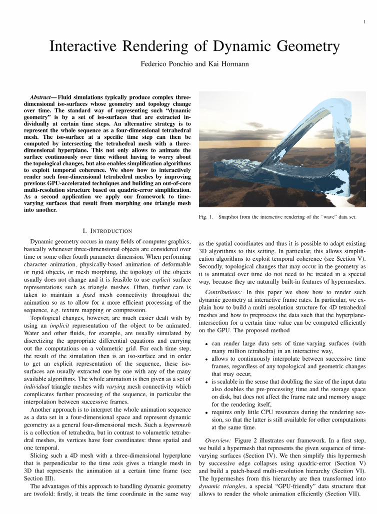
1

Interactive Rendering of Dynamic GeometryFederico Ponchio and Kai Hormann

Abstract— Fluid simulations typically produce complex three-dimensional iso-surfaces whose geometry and topology changeover time. The standard way of representing such “dynamicgeometry” is by a set of iso-surfaces that are extracted in-dividually at certain time steps. An alternative strategy is torepresent the whole sequence as a four-dimensional tetrahedralmesh. The iso-surface at a specific time step can then becomputed by intersecting the tetrahedral mesh with a three-dimensional hyperplane. This not only allows to animate thesurface continuously over time without having to worry aboutthe topological changes, but also enables simplification algorithmsto exploit temporal coherence. We show how to interactivelyrender such four-dimensional tetrahedral meshes by improvingprevious GPU-accelerated techniques and building an out-of-coremulti-resolution structure based on quadric-error simplification.As a second application we apply our framework to time-varying surfaces that result from morphing one triangle meshinto another.

I. INTRODUCTION

Dynamic geometry occurs in many fields of computer graphics,basically whenever three-dimensional objects are considered overtime or some other fourth parameter dimension. When performingcharacter animation, physically-based animation of deformableor rigid objects, or mesh morphing, the topology of the objectsusually does not change and it is feasible to use explicit surfacerepresentations such as triangle meshes. Often, further care istaken to maintain a fixed mesh connectivity throughout theanimation so as to allow for a more efficient processing of thesequence, e.g. texture mapping or compression.

Topological changes, however, are much easier dealt with byusing an implicit representation of the object to be animated.Water and other fluids, for example, are usually simulated bydiscretizing the appropriate differential equations and carryingout the computations on a volumetric grid. For each time step,the result of the simulation then is an iso-surface and in orderto get an explicit representation of the sequence, these iso-surfaces are usually extracted one by one with any of the manyavailable algorithms. The whole animation is then given as a set ofindividual triangle meshes with varying mesh connectivity whichcomplicates further processing of the sequence, in particular theinterpolation between successive frames.

Another approach is to interpret the whole animation sequenceas a data set in a four-dimensional space and represent dynamicgeometry as a general four-dimensional mesh. Such a hypermeshis a collection of tetrahedra, but in contrast to volumetric tetrahe-dral meshes, its vertices have four coordinates: three spatial andone temporal.

Slicing such a 4D mesh with a three-dimensional hyperplanethat is perpendicular to the time axis gives a triangle mesh in3D that represents the animation at a certain time frame (seeSection III).

The advantages of this approach to handling dynamic geometryare twofold: firstly, it treats the time coordinate in the same way

Fig. 1. Snapshot from the interactive rendering of the “wave” data set.

as the spatial coordinates and thus it is possible to adapt existing3D algorithms to this setting. In particular, this allows simplifi-cation algorithms to exploit temporal coherence (see Section V).Secondly, topological changes that may occur in the geometry asit is animated over time do not need to be treated in a specialway, because they are naturally built-in features of hypermeshes.

Contributions: In this paper we show how to render suchdynamic geometry at interactive frame rates. In particular, we ex-plain how to build a multi-resolution structure for 4D tetrahedralmeshes and how to preprocess the data such that the hyperplane-intersection for a certain time value can be computed efficientlyon the GPU. The proposed method

• can render large data sets of time-varying surfaces (withmany million tetrahedra) in an interactive way,

• allows to continuously interpolate between successive timeframes, regardless of any topological and geometric changesthat may occur,

• is scalable in the sense that doubling the size of the input dataalso doubles the pre-processing time and the storage spaceon disk, but does not affect the frame rate and memory usagefor the rendering itself,

• requires only little CPU resources during the rendering ses-sion, so that the latter is still available for other computationsat the same time.

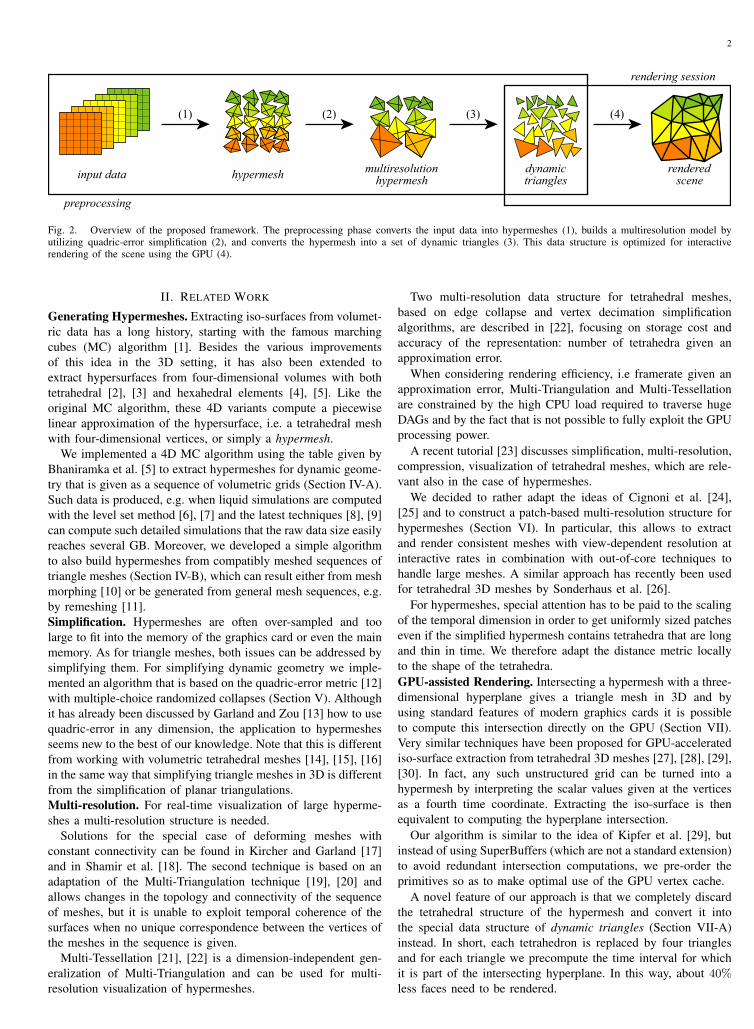
Overview: Figure 2 illustrates our framework. In a first step,we build a hypermesh that represents the given sequence of time-varying surfaces (Section IV). We then simplify this hypermeshby successive edge collapses using quadric-error (Section V)and build a patch-based multi-resolution hierarchy (Section VI).The hypermeshes from this hierarchy are then transformed intodynamic triangles, a special “GPU-friendly” data structure thatallows to render the whole animation efficiently (Section VII).

2

input data hypermesh multiresolutionhypermesh

dynamictriangles

renderedscene

rendering session

preprocessing

(1) (2) (3) (4)

Fig. 2. Overview of the proposed framework. The preprocessing phase converts the input data into hypermeshes (1), builds a multiresolution model byutilizing quadric-error simplification (2), and converts the hypermesh into a set of dynamic triangles (3). This data structure is optimized for interactiverendering of the scene using the GPU (4).

II. RELATED WORK

Generating Hypermeshes. Extracting iso-surfaces from volumet-ric data has a long history, starting with the famous marchingcubes (MC) algorithm [1]. Besides the various improvementsof this idea in the 3D setting, it has also been extended toextract hypersurfaces from four-dimensional volumes with bothtetrahedral [2], [3] and hexahedral elements [4], [5]. Like theoriginal MC algorithm, these 4D variants compute a piecewiselinear approximation of the hypersurface, i.e. a tetrahedral meshwith four-dimensional vertices, or simply a hypermesh.

We implemented a 4D MC algorithm using the table given byBhaniramka et al. [5] to extract hypermeshes for dynamic geome-try that is given as a sequence of volumetric grids (Section IV-A).Such data is produced, e.g. when liquid simulations are computedwith the level set method [6], [7] and the latest techniques [8], [9]can compute such detailed simulations that the raw data size easilyreaches several GB. Moreover, we developed a simple algorithmto also build hypermeshes from compatibly meshed sequences oftriangle meshes (Section IV-B), which can result either from meshmorphing [10] or be generated from general mesh sequences, e.g.by remeshing [11].Simplification. Hypermeshes are often over-sampled and toolarge to fit into the memory of the graphics card or even the mainmemory. As for triangle meshes, both issues can be addressed bysimplifying them. For simplifying dynamic geometry we imple-mented an algorithm that is based on the quadric-error metric [12]with multiple-choice randomized collapses (Section V). Althoughit has already been discussed by Garland and Zou [13] how to usequadric-error in any dimension, the application to hypermeshesseems new to the best of our knowledge. Note that this is differentfrom working with volumetric tetrahedral meshes [14], [15], [16]in the same way that simplifying triangle meshes in 3D is differentfrom the simplification of planar triangulations.Multi-resolution. For real-time visualization of large hyperme-shes a multi-resolution structure is needed.

Solutions for the special case of deforming meshes withconstant connectivity can be found in Kircher and Garland [17]and in Shamir et al. [18]. The second technique is based on anadaptation of the Multi-Triangulation technique [19], [20] andallows changes in the topology and connectivity of the sequenceof meshes, but it is unable to exploit temporal coherence of thesurfaces when no unique correspondence between the vertices ofthe meshes in the sequence is given.

Multi-Tessellation [21], [22] is a dimension-independent gen-eralization of Multi-Triangulation and can be used for multi-resolution visualization of hypermeshes.

Two multi-resolution data structure for tetrahedral meshes,based on edge collapse and vertex decimation simplificationalgorithms, are described in [22], focusing on storage cost andaccuracy of the representation: number of tetrahedra given anapproximation error.

When considering rendering efficiency, i.e framerate given anapproximation error, Multi-Triangulation and Multi-Tessellationare constrained by the high CPU load required to traverse hugeDAGs and by the fact that is not possible to fully exploit the GPUprocessing power.

A recent tutorial [23] discusses simplification, multi-resolution,compression, visualization of tetrahedral meshes, which are rele-vant also in the case of hypermeshes.

We decided to rather adapt the ideas of Cignoni et al. [24],[25] and to construct a patch-based multi-resolution structure forhypermeshes (Section VI). In particular, this allows to extractand render consistent meshes with view-dependent resolution atinteractive rates in combination with out-of-core techniques tohandle large meshes. A similar approach has recently been usedfor tetrahedral 3D meshes by Sonderhaus et al. [26].

For hypermeshes, special attention has to be paid to the scalingof the temporal dimension in order to get uniformly sized patcheseven if the simplified hypermesh contains tetrahedra that are longand thin in time. We therefore adapt the distance metric locallyto the shape of the tetrahedra.GPU-assisted Rendering. Intersecting a hypermesh with a three-dimensional hyperplane gives a triangle mesh in 3D and byusing standard features of modern graphics cards it is possibleto compute this intersection directly on the GPU (Section VII).Very similar techniques have been proposed for GPU-acceleratediso-surface extraction from tetrahedral 3D meshes [27], [28], [29],[30]. In fact, any such unstructured grid can be turned into ahypermesh by interpreting the scalar values given at the verticesas a fourth time coordinate. Extracting the iso-surface is thenequivalent to computing the hyperplane intersection.

Our algorithm is similar to the idea of Kipfer et al. [29], butinstead of using SuperBuffers (which are not a standard extension)to avoid redundant intersection computations, we pre-order theprimitives so as to make optimal use of the GPU vertex cache.

A novel feature of our approach is that we completely discardthe tetrahedral structure of the hypermesh and convert it intothe special data structure of dynamic triangles (Section VII-A)instead. In short, each tetrahedron is replaced by four trianglesand for each triangle we precompute the time interval for whichit is part of the intersecting hyperplane. In this way, about 40%

less faces need to be rendered.

3

Volume Visualization. A completely different approach to ren-dering iso-surfaces from four-dimensional volumes is by directvolume visualization. In order to handle large data sets, the latestof these techniques preprocess the data by a clever use of TSPtree data structures [31] and wavelet transforms [32], [33], butfor the data size that we consider, they cannot achieve interactiveframe rates on a single PC, at least not yet [34], [35].

III. HYPERMESHES IN 4D

The concept of embedding an animated sequence of objectsin a space with one more dimension is certainly not new, butnevertheless let us quickly review and formalize the basics.

Assume that we are given for any parameter t ∈ R a curveC(t) ⊂ R2 in the plane. Then by adding t as a third coordinate,we can represent the union of all C(t) as a 3D object,

C = {(C(t), t) : t ∈ R} ⊂ R3.

More precisely, C is a two-dimensional surface in 3D. Slicingthis surface with the plane P (t) = {(x, y, t) : (x, y) ∈ R2} thatis orthogonal to the t-axis just gives back the curve at parametervalue t,

C ∩ P (t) = C(t).

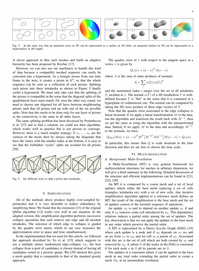
Figure 3 (left) illustrates this concept.Likewise we can embed a sequence of surfaces S(t) ⊂ R3 into

R4 to give the hypersurface

S = {(S(t), t) : t ∈ R} ⊂ R4.

Again, intersecting S with a t-orthogonal hyperplane gives backthe surface S(t); see Figure 3 (right) for an example.

In the same way that it is common to use triangle meshesto describe surfaces in 3D, it is also natural to represent ahypersurface in 4D as a tetrahedral hypermesh H . In contrastto volumetric tetrahedral meshes, the vertices vi = (xi, yi, zi, ti)

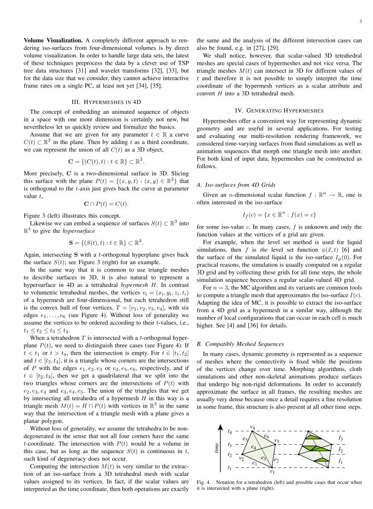
of a hypermesh are four-dimensional, but each tetrahedron stillis the convex hull of four vertices, T = [v1, v2, v3, v4], with sixedges e1, . . . , e6 (see Figure 4). Without loss of generality weassume the vertices to be ordered according to their t-values, i.e.,t1 ≤ t2 ≤ t3 ≤ t4.

When a tetrahedron T is intersected with a t-orthogonal hyper-plane P (t), we need to distinguish three cases (see Figure 4). Ift < t1 or t > t4, then the intersection is empty. For t ∈ [t1, t2]

and t ∈ [t3, t4], it is a triangle whose corners are the intersectionsof P with the edges e1, e2, e3 or e3, e5, e6, respectively, and ift ∈ [t2, t3], then we get a quadrilateral that we split into thetwo triangles whose corners are the intersections of P (t) withe2, e3, e4 and e3, e4, e5. The union of the triangles that we getby intersecting all tetrahedra of a hypermesh H in this way is atriangle mesh M(t) = H ∩ P (t) with vertices in R3 in the sameway that the intersection of a triangle mesh with a plane gives aplanar polygon.

Without loss of generality, we assume the tetrahedra to be non-degenerated in the sense that not all four corners have the samet-coordinate. The intersection with P (t) would be a volume inthis case, but as long as the sequence S(t) is continuous in t,such kind of degeneracy does not occur.

Computing the intersection M(t) is very similar to the extrac-tion of an iso-surface from a 3D tetrahedral mesh with scalarvalues assigned to its vertices. In fact, if the scalar values areinterpreted as the time coordinate, then both operations are exactly

the same and the analysis of the different intersection cases canalso be found, e.g. in [27], [29].

We shall notice, however, that scalar-valued 3D tetrahedralmeshes are special cases of hypermeshes and not vice versa. Thetriangle meshes M(t) can intersect in 3D for different values oft and therefore it is not possible to simply interpret the timecoordinate of the hypermesh vertices as a scalar attribute andconvert H into a 3D tetrahedral mesh.

IV. GENERATING HYPERMESHES

Hypermeshes offer a convenient way for representing dynamicgeometry and are useful in several applications. For testingand evaluating our multi-resolution rendering framework, weconsidered time-varying surfaces from fluid simulations as well asanimation sequences that morph one triangle mesh into another.For both kind of input data, hypermeshes can be constructed asfollows.

A. Iso-surfaces from 4D Grids

Given an n-dimensional scalar function f : Rn → R, one isoften interested in the iso-surface

If (c) = {x ∈ Rn : f(x) = c}

for some iso-value c. In many cases, f is unknown and only thefunction values at the vertices of a grid are given.

For example, when the level set method is used for liquidsimulations, then f is the level set function φ(~x, t) [6] andthe surface of the simulated liquid is the iso-surface Iφ(0). Forpractical reasons, the simulation is usually computed on a regular3D grid and by collecting these grids for all time steps, the wholesimulation sequence becomes a regular scalar-valued 4D grid.

For n = 3, the MC algorithm and its variants are common toolsto compute a triangle mesh that approximates the iso-surface I(c).Adapting the idea of MC, it is possible to extract the iso-surfacefrom a 4D grid as a hypermesh in a similar way, although thenumber of local configurations that can occur in each cell is muchhigher. See [4] and [36] for details.

B. Compatibly Meshed Sequences

In many cases, dynamic geometry is represented as a sequenceof meshes where the connectivity is fixed while the positionsof the vertices change over time. Morphing algorithms, clothsimulations and other non-skeletal animations produce surfacesthat undergo big non-rigid deformations. In order to accuratelyapproximate the surface in all frames, the resulting meshes areusually very dense because once a detail requires a fine resolutionin some frame, this structure is also present at all other time steps.

v1

v3

v4

v2 e2e1

e5e6

e4e3

t1

t3

t4

t2I1

I3

I2time

Fig. 4. Notation for a tetrahedron (left) and possible cases that occur whenit is intersected with a plane (right).

4

t = 0.2 t = 0.6 t = 1.6

t = 4.0 t = 3.9 t = 3.0

t = 0.2 t = 0.6 t = 1.6

t = 2.0 t = 2.1 t = 3.0

Fig. 3. In the same way that an animated curve in 2D can be represented as a surface in 3D (left), an animated surface in 3D can be represented as ahypersurface in 4D (right).

A clever approach to thin such meshes and build an adaptivehierarchy has been proposed by Kircher [17].

However, we can also use our machinery to handle this kindof data because a compatibly meshed sequence can easily beconverted into a hypermesh. As a triangle moves from one timeframe to the next, it creates a prism in R4, so that the wholesequence can be seen as a collection of such prisms. Splittingeach prism into three tetrahedra as shown in Figure 5 finallyyields a hypermesh. We must only take care that the splitting ofthe prisms is compatible in the sense that the diagonal splits of thequadrilateral faces must match. Or, seen the other way round, weneed to choose one diagonal for all faces between neighbouringprisms such that all prisms end up with one of the six possiblesplits. Note that this needs to be done only for one layer of prismsas the connectivity is the same in all other layers.

The same splitting problem has been discussed by Porumbescuet al. [37] and to find a solution, we could use their algorithm,which works well in practice but is not proven to converge.However, there is a much simpler strategy: if v1, . . . , vn are thevertices of the mesh, then by always taking the diagonals thathave the vertex with the smaller index at the bottom, it is easy tosee that the forbidden “cyclic” splits are avoided for all prisms[38].

Fig. 5. Six different ways to split a prism into tetrahedra.

V. SIMPLIFICATION

All of the methods above produce highly over-sampled hy-permeshes and it is very desirable to reduce redundancy bysimplifying them. We found that the extension [13] of the originalQSlim algorithm [12] works very well in our situation. In theadapted version, this simplification algorithm performs successivecollapse operations that each remove one edge and all incidenttetrahedra. The selection of which edge to collapse is guidedby the quadric error metric which in our case measures theapproximation error in space and time simultaneously.

In the implementation that we used for this article, we followedthe approach described by Vo et al. [15] which suggests touse a multiple choice randomized edge-collapse: i.e., the bestcollapse from a pool of candidates is chosen instead of having allcandidates sorted in a priority queue. Wu [39] showed this givesa mesh quality that is comparable to that of the standard greedyapproach.

The quadric error of x with respect to the tangent space at avertex v is given by

Qv(x) = (x− v)TA(x− v)

where A is the sum of outer products of normals,

A =Xi

n(Ti)n(Ti)T

and the summation index i ranges over the set of all tetrahedraTi incident to v. The normal n(T ) of a 4D tetrahedron T is well-defined because T is “flat” in the sense that it is contained in ahyperplane of codimension one. The normal can be computed bytaking the 4D cross product of three edge vectors of T .

Note that the quadric error associated to the edge collapses islinear invariant: if we apply a linear transformation M to the data,run the algorithm and transform the result back with M−1, thenwe get the same as using the algorithm with the untransformeddata. Indeed, if we apply M to the data and accordingly M−T

to the normals, we have

QMv(Mx) = (x− v)TMT ˆM−TAM−1˜M(x− v) = Qv(x).

In particular, this means that Q is scale invariant in the timedirection and thus we are free to choose the time scale.

VI. MULTI-RESOLUTION

A. Background: Multi-Tessellation

A Multi-Tessellation (MT) is very general framework formultiresolution structures for meshes in arbitrary dimension, wewill give a brief summary in the following. Detailed discussion ofthe structure and efficient implementations can be found in [21],[22], [20].

An MT it is composed by a coarse mesh and a set of localupdates which refine the base mesh replacing a set of cells(triangles, tetrahedra etc) with a set of new cells. Any iterativesimplification algorithm applied to a reference mesh defines anMT: the result of the simplification is the base mesh and the setof updates consist of the inverted sequence of operations.

An update u2 is said to depend on another update u1 if andonly if u2 removes some cell introduced by u1. This dependencyrelations induces a partial order among the set of updates. Thekey observation is that we can apply the updates to the base meshin any order which preserve the partial order.

A MT is represented by a Direct Acyclic Graph (DAG) [19]where each update is a node and if u2 depends on u1 we addan arc from u1 to u2, and we call u1 a parent of u2. Associatedwith this arc is the set of cell which are both created by u1 andremoved by u2. A subset S of the nodes in the DAG is consistentif for each node u in S all its parents are in S.

The updates in a consistent subset S can be applied to the basemesh in any total order extending the partial order to create amesh MS at an intermediate resolution.

5

The collection of arcs CS from nodes in S to nodes not in S

is called a cut of the DAG, and MS is exactly the collection ofcells associated with all the arcs in CS .

We can associate with every update, and so to every node in theDAG, an approximation error. The rendering algorithm performa traversal of the DAG to select a cut which minimizes the errorgiven a maximum number of resulting cells. Different metrics canbe implemented to calculate the error and additional constrainscan be imposed on the traversal.

B. Patch-based Multi-Tessellation

Usually the update operation in an MT correspond to the atomicoperation of an edge-collapse or vertex-removal operation. Thisensure maximum granularity and smooth transaction betweendifferent resolutions, but result in very large DAGs which requireCPU intensive computations in the rendering phase.

Due to the fact that GPU speed is increasing at a much fasterrate than CPU speed, an established trend in multi-resolutionalgorithms for meshes [40] is to increase the number of trianglesaffected by an update operation, moving the refine-coarsen deci-sions from the level of a single triangle to blocks of triangles. Thishas the advantage of removing the CPU bottleneck and maximallyutilizing the processing power of the GPU. This approach canfurther be supported by preprocessing the data such that it ishandled most efficiently by the GPU. The loss in granularity iscompensated by a much higher triangle per second rendering rate.

Cignoni et al. [25] presented a multi-resolution frameworkwhich combines this concept with the ideas of multi-triangulations[20] and we extended it so that it can be used for hypermeshes. Inthe following we give only a brief description of the approach andin particular the requirements for adapting it to hypermeshes. Formore details on this subject we refer to [25] and the referencescited therein.

C. Building the Multi-resolution Model

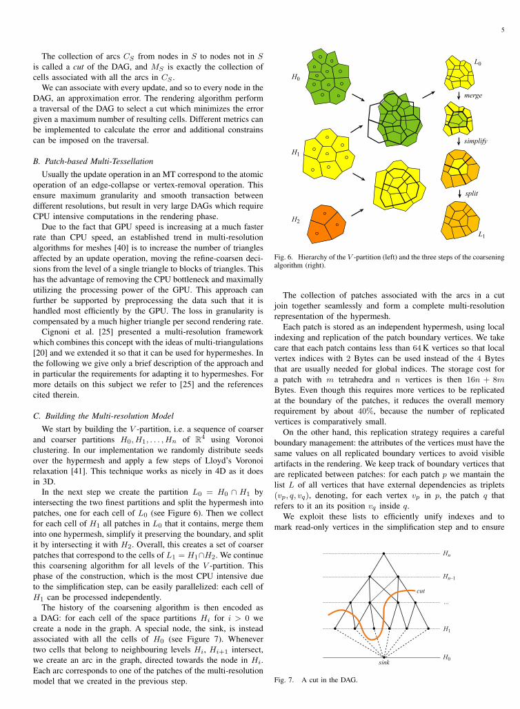
We start by building the V -partition, i.e. a sequence of coarserand coarser partitions H0, H1, . . . , Hn of R4 using Voronoiclustering. In our implementation we randomly distribute seedsover the hypermesh and apply a few steps of Lloyd’s Voronoirelaxation [41]. This technique works as nicely in 4D as it doesin 3D.

In the next step we create the partition L0 = H0 ∩ H1 byintersecting the two finest partitions and split the hypermesh intopatches, one for each cell of L0 (see Figure 6). Then we collectfor each cell of H1 all patches in L0 that it contains, merge theminto one hypermesh, simplify it preserving the boundary, and splitit by intersecting it with H2. Overall, this creates a set of coarserpatches that correspond to the cells of L1 = H1∩H2. We continuethis coarsening algorithm for all levels of the V -partition. Thisphase of the construction, which is the most CPU intensive dueto the simplification step, can be easily parallelized: each cell ofH1 can be processed independently.

The history of the coarsening algorithm is then encoded asa DAG: for each cell of the space partitions Hi for i > 0 wecreate a node in the graph. A special node, the sink, is insteadassociated with all the cells of H0 (see Figure 7). Whenevertwo cells that belong to neighbouring levels Hi, Hi+1 intersect,we create an arc in the graph, directed towards the node in Hi.Each arc corresponds to one of the patches of the multi-resolutionmodel that we created in the previous step.

merge

simplify

split

H0

H1

H2

L0

L1

Fig. 6. Hierarchy of the V -partition (left) and the three steps of the coarseningalgorithm (right).

The collection of patches associated with the arcs in a cutjoin together seamlessly and form a complete multi-resolutionrepresentation of the hypermesh.

Each patch is stored as an independent hypermesh, using localindexing and replication of the patch boundary vertices. We takecare that each patch contains less than 64 K vertices so that localvertex indices with 2 Bytes can be used instead of the 4 Bytesthat are usually needed for global indices. The storage cost fora patch with m tetrahedra and n vertices is then 16n + 8m

Bytes. Even though this requires more vertices to be replicatedat the boundary of the patches, it reduces the overall memoryrequirement by about 40%, because the number of replicatedvertices is comparatively small.

On the other hand, this replication strategy requires a carefulboundary management: the attributes of the vertices must have thesame values on all replicated boundary vertices to avoid visibleartifacts in the rendering. We keep track of boundary vertices thatare replicated between patches: for each patch p we mantain thelist L of all vertices that have external dependencies as triplets(vp, q, vq), denoting, for each vertex vp in p, the patch q thatrefers to it an its position vq inside q.

We exploit these lists to efficiently unify indexes and tomark read-only vertices in the simplification step and to ensure

Hn

Hn–1

…

H1

H0sink

cut

Fig. 7. A cut in the DAG.

6

consistency of vertex attributes.For example, to compute the 4D normals, we start at the finest

level and propagate the ones at the boundary vertices to the nextcoarser level and then repeat the process up to the coarsest level.This data is not needed for rendering and can be discarded at theend of the preprocessing.

The set of patches is easily managed out-of-core: each patch,along with its boundary information, is stored sequentially on diskand memory mapped individually when needed. This approachis somewhat independent from how patches are actually storedand allow to use the same structure for rendering. In this caseeach patch is further preprocessed for GPU-assisted rendering asdescribed in Section VII-A.

Finally, we store the DAG and an array of entries that containsfor each patch in the data set the number of faces and vertices, theoffset and size on the disk, the bounding sphere, and the estimatedgeometric error.

The are several different structures to encode the DAG [19],[20] with various tradeoff between space and speed, but given thelimited size of the DAG due to the cluster structure, this is not acritical part of the rendering algorithm. This information is smallenough to be kept in RAM even for very large models.

The overall storage cost of this structure is around 120n Byteswhere n is the number of vertices in the reference mesh, while theoverhead of the DAG storage and vertex replication is neglicible.By comparison the explicit data structure for tetrahedral MTdescribed in [22] requires from 450n to 880n Bytes. This is dueto the reduced granularity and expressive power.

The Edge-Base MT also described in [22] requires 36n Bytes.It is however a compressed format which requires a substantiallyhigher computational cost respect to the explicit structure. Com-pression of topological information in tetrahedral meshes [42]achieves approximatively 3 Bytes per tetrahedra (or 0.6 Bytes pervertex) on small meshes. If we were to compress each patch theoverall cost would be 34n Bytes, with the advantage that it wouldbe trivial to parallelize the compression/decompression threads.

Notice how the structure of the DAG is effectively decoupledfrom the choice of the simplification algorithm and the mesh rep-resentation. As long as the boundary of a patch is preserved anyalgorithm (edge-collapse, vertex removal, remeshing, clusteringetc.) could be applied.

D. Differences between 3D and 4D

In general, the ratio between the size of the boundary and theinterior of an n-dimensional object grows with n. Therefore, thepatches of a hypermesh have on average much more boundaryvertices than those of a triangle mesh. Thus, it is crucial to keepthe patches well-shaped, because otherwise it may quickly happenduring the construction of the hierarchy that the patches consistof mostly boundary vertices and cannot be simplified any further.

For dynamic geometry, one important factor that has a biginfluence on the shape of the patches is how the time unit isrelated to the three spatial units, because we measure distanceswith the standard Euclidean norm in 4D. Decreasing the timescale makes the patches longer and thinner in time and vice versa,and we would like to find the “correct” scale that gives patchesas uniformly sized as possible. Note that choosing the time scaledoes not affect the simplification process (see Section V).

For data from the 4D MC algorithm, the obvious choice is to setthe time between two frames equal to the size of the marching

cube. However, during the simplification process, tetrahedra insurface regions that move little, become elongated in the timedirection. During the Lloyd relaxation we therefore use for everyVoronoi cell an individual distance norm that weights the timedirection such that the average shape of the tetrahedra in that cellis uniform in all directions with respect to this norm. Of course,the same idea could also be used in the 3D setting, but for surfacesit is much less crucial to have well-shaped patches.

E. Rendering the Multi-resolution Model

The goal of the rendering algorithm is to select a cut in theDAG to adapt the resolution in different parts of the model suchthat the error in screen-space is as uniform and low as possibleand to maintain the visualization interactive, while constrained bythe resources that are available: disk-speed, RAM, video-RAM,CPU budget and GPU budget.

The screen-space error for a patch is computed as follows:if the bounding sphere is outside of the 4D viewing frustum, theerror is set to zero, if the viewpoint is inside the bounding sphere,the error is infinite, otherwise we divide the geometric error bythe distance from the viewpoint to the bounding sphere. As aresult, regions that are further away from the viewer require alower resolution than those that are close to the camera. Notethat the word “distance” refers to the 4D distance and includesthe temporal dimension. The error associated with a cut in theDAG is the maximum error of the collection of patches selectedby the cut.

For each frame, the algorithm updates the cut in the DAGby performing refining or coarsening operations that correspondto moving the cut up or down in the tree. We associate witheach refining or coarsening operation an error: the maximumerror among the new selected patches. Each refinement operationconsumes resources such as disk, RAM, video-RAM and GPUbudget, while coarsening operations release them.

The algorithm maintains a list of possible refinement andcoarsening operations sorted by the error associated with them.Refinement operations, starting from the greatest error, are carriedout as long as free resources exists and coarsening operations,starting from the lowest error are performed to free resources. Theprocedure terminates when the budget is used up and the smallesterror in the coarsening list is bigger than the biggest error in therefining list, i.e., we would need to increase the overall error tofree resources.

A detailed description of the algorithm can be found in [24,Section 4.3], the structure of the DAG being identical. Theimplementation is described in detail in [25, Section 5]: inparticular disk, RAM and video-RAM are treated like a multi-level cache accessed by a prefetching routine, executed in parallelwith the rendering routine.

VII. GPU-ASSISTED RENDERING

The basic algorithm for rendering a hypermesh at a certaintime-coordinate t is to slice all tetrahedra with the hyperplanethat intersects the time axis at t and is perpendicular to it (seeSection III). But doing this in the CPU and sending the resultingtriangles to the graphics card is inefficient because the CPU ismuch slower in processing geometry than the GPU. There exista few techniques to perform these computations on the GPU andeach one could be used to render the patches of the multiresolutionstructure, while offering different space-speed tradeoffs.

7

vertex andnormal textures

edge table

triangle table

interval table t1 t5t4 t6t3 t2 t6

e1 e4e2 e3e2 e3 e4 e5 e3

v1 v2v1 v4v2 v1 v3 v3 v2

e3

v1

v4

v2 v3

v6v5

n1

n4

n2 n3

n6n5

• • •

• • •

• • •

• •• •

• • • • • •

• •• •

• • • • • •

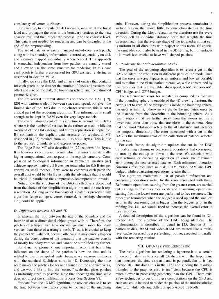
Fig. 8. Data structures used for GPU rendering.

The technique of Pascucci [27] basically processes a quad foreach tetrahedron by storing the coordinates of the four verticesin the vertex attributes of each vertex of the tetrahedron andperforming a marching tetrahedra on-the-fly. It is very fast but themultiple replication of the vertex coordinates makes it impracticalfor big datasets, due to the memory overhead. Buatois et al. [30]avoid this replication by storing the tetrahedral indexed structurein textures and using the texture access capability of the vertexshader. Unfortunately, the access to the vertex texture is quiteslow in current graphics cards and this technique requires 20accesses per tetrahedron. Kipfer et al. [29] developed an edge-based approach, whose main strength is that it avoids redundantcomputations of edge-surface intersections. This technique, how-ever, takes advantage of a specific feature of a single graphicscard vendor: the SuperBuffer extension of ATI cards.

We developed yet another strategy which is tailored to ourspecific needs, in particular it is faster than [30] while requiringmore space. In Section VIII we compare the performances of thetwo techniques.

A. Dynamic Triangles

As described in Section III, three cases need to be distinguishedwhen the hyperplane P (t) intersects a tetrahedron T , and fourdifferent kind of triangles can occur. We store all of these fourtriangles as dynamic triangles in the sense that each triangle isassociated with a “lifespan” and the three edges on which itsvertices lie. In the notation of Figure 4, the first triangle “lives”during the time interval I1 = [t1, t2] with vertices on the edgese1, e2, e3 and likewise for the other three triangles, so that westore

41 := {I1, (e1, e2, e3)}, 42 := {I2, (e2, e3, e4)},43 := {I2, (e3, e4, e5)}, 44 := {I3, (e3, e5, e6)}

for each tetrahedron of the hypermesh H .Like [29] we further build an edge table for the edges of

all tetrahedra. In this table, each edge e = [vi, vj ] is stored asa pair of indices (i, j) to the vertices that this edge connects.We can now discard the hypermesh data structure because thedynamic triangles, the edge table, and the vertex list contain allthe necessary information needed for computing the triangle meshM(t) = H ∩ P (t) for any given time parameter t on the GPU.

Suppose that t ∈ I for some triangle 4 = {I, (e1, e2, e3)}from the tetrahedron T . For each corner we then use the edgetable to look up the indices of the two endpoints v1 and v2 andread their coordinates from the vertex list. We finally interpolatethe (x, y, z)-coordinates of v1 and v2 linearly with the weightλ = (t − t1)/(t2 − t1) to get the 3D position of the triangleT ∩ P (t) ∈M(t).

In order to implement this strategy in OpenGL westore the 4D coordinates of the vertices in an RGBAtexture and use vertex buffers to store the triangle ta-ble (ELEMENT ARRAY BUFFER ARB) and the edge table(ARRAY BUFFER ARB). The function call “glDrawElements”takes triples of indices from the triangle table and feeds thecorresponding values from the edge table to the vertex program,which in turn uses these values to look up the coordinates ofthe edge endpoints in the texture. It then interpolates them toget the actual 3D coordinates of the corner (see Figure 8). Notethat any vertex attribute can be treated in the same way as thevertices themselves by storing them in additional textures. In ourimplementation we did this for normals to enable Phong shadingand refraction.

We can detect in the vertex program if the lifespan I of atriangle does not contains the current t: the parameter λ for thelinear interpolation is negative or bigger than 1 for one of itscorners. We can easily cull the triangle by moving the vertexposition to the viewpoint so that the whole triangle becomesinvisible.

Usually a large fraction of the triangles have a lifespan I thatdoes not contains the current t and we would like to process inthe GPU only the active ones.

Computing the active triangles requires a lot of CPU compu-tations and sending the primitives to the graphics card for eachframe requires a lot of bandwidth.

It is more efficient to sort the triangles according to the centreof their lifespan, store them on the graphics card as elementarray buffers and only process the interval that contains the activetriangles. In this way we process a certain number of non-activetriangles, but each primitive is transferred to the graphics cardonly once.

A simple solution is to subdivide the global lifespan of thepatch into n regular intervals and store for each interval theindices of the first and last triangle that intersect the interval. Thenumber of intervals compromises between accuracy and space.

The problem with this solution is that the dynamic trianglesin the patch have lifespans that vary considerably in length.Regardless of the sorting order, the interval that contains theactive triangles will usually contain many non-active triangles,which results in a quite inefficient culling.

To prevent this, we group intervals of approximate equal lengthtogether in a few “bands” and apply the simple solution abovefor each band (see Figure 10). This results in more calls of“glDrawRangeElements” (one per band) but greatly improves theculling efficiency. The most appropriate number of bands dependson the relative cost of calling “glDrawRangeElements” versus thatof rendering a tetrahedron.

Another solution is to use an interval tree to compute the activetriangles and compact the list into a few intervals such that nointerval contains a long sequence of non-active triangles. This ismore robust with respect to irregular distributions of lifespans andmore accurate, but it also requires more space (O(n)) and it iscomputationally more expensive: O(logN +m), where m is thenumber of active triangles.

In our examples, we experienced that about 10% of all trianglesare active for each frame on average. The single-band approachtypically requires to process approximately 5 times as manytriangles as needed, but only 1 out of 5 triangles are actuallyrendered by the vertex shader. Instead, when using 4 to 6 bands

8

e2

e1e4

e3t1

t3

t4

t2time

q

p

e0

e2

e1e4

e3 e2

e1e4

e3

qp

e0

e2

e1e4

e3

qp

q

p

pmax

qmax

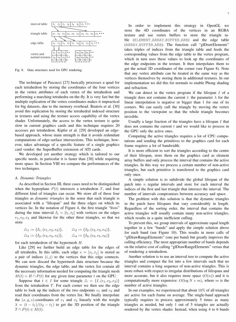
Fig. 9. An edge collapse in the triangle mesh M(t) (green) is equivalent to joining two faces of the hypermesh (light green).

and a number of regular intervals equal to a quarter of the numberof tetrahedra, this rate improved to 3 out of 4 triangles on averagein all our examples. The space overhead for this banded structureis 4 bytes per tetrahedron.

B. Optimizing Dynamic Triangles

Overall, the space needed to store the dynamic triangles ex-ceeds that of the indexed hypermesh by about 65%, but we canuse two approaches to reduce this number.

Whenever two or more vertices of a tetrahedron T havethe same time coordinate, some of the intervals I1, I2, I3 areempty and the corresponding dynamic triangles and edges canbe removed from the lists. Thus, upon simplification of the mesh(see Section V) we try to align as many vertices as possible intime. This typically removes about 20% of all dynamic triangles.

Another idea to reduce the number of dynamic triangles isbased on the observation that the triangle mesh M(t) containsmany thin triangles which contribute little to the geometric shape.Thus, if we were to apply a quadric-error simplification algorithmon M(t), we would reduce the number of triangles considerablywithout significantly increasing the error.

As shown in Figure 9, collapsing an edge of M(t) is equivalentto removing an edge from the hypermesh H and combining twofaces to form a quadrilateral. In this example, collapsing the vertexp into q removes two faces from M(t), the edge e0 from H andforms the quadrilateral with edges e1, . . . , e4. At the same time,the tetrahedra adjacent to edge e0 are combined to a volumetricelement that is not a tetrahedron (see Figure 11).

begin

end

t

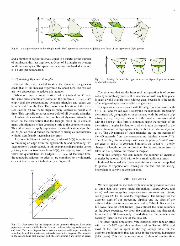
Fig. 10. Span space for the lifespans of the dynamic triangles: Each pointrepresents an interval with the abscissa and ordinate referring to the start andend time. The three diagonal bands contain intervals with approximately thesame length, with the short-living intervals close to the diagonal. The intervalsin the second band that intersect with the current time t are shown in green.

time

Fig. 11. Joining faces of the hypermesh as in Figure 9 generates non-tetrahedral elements.

The structure that results from such an operation is of coursenot a hypermesh anymore, still its intersection with any time planeis again a valid triangle mesh without gaps, because it is the resultof an edge-collapse over a valid triangle mesh.

The quadric error associated with this edge collapse varies witht ∈ [t1, t4] and we can easily determine the maximum: Regardingthe surface M , the quadric error associated with the collapse of pinto q is (p−q)TA(p−q), where A is the quadric form associatedwith the point p. This form is computed using the normals of allthe surface triangles incident to it, which in turn correspond to theintersections of the hyperplane P (t) with the tetrahedra adjacentto e0. The 3D normals of these triangles are the projections ofthe 4D normals from the corresponding tetrahedra onto P (t).Therefore, they do not change with t as the point p “slides” overthe edge e0 and A is constant. Similarly, the vector p − q onlychanges in length but not in direction. So the maximum error istaken at t = t1 where the vector is longest.

With this strategy, we can reduce the number of dynamictriangles by another 30% with only a small additional error.

It should be noted that these optimizations cannot be appliedto general 4D applications, relying on the fact that the slicinghyperplane is always at constant time.

VIII. EXAMPLES

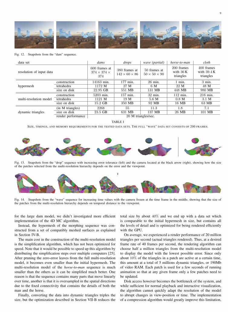
We have applied the methods explained in the previous sectionsto three data sets: three liquid simulations (dams, drops, andwave) and two morphing sequences (horse-to-man and cloth);see Figures 12, 13, 14, and 15, respectively. The timings for thedifferent steps of our processing pipeline and the sizes of thedifferent data structures are summarized in Table I. Because thefull wave data set (200 frames) gives almost the same numbersas the drops sequence, we show the timings and size that resultfrom the first 50 frames only to underline that the numbers arebasically linear in the size of the data set.

The three liquid simulations were extracted from regular gridswith the 4D MC algorithm as described in Section IV-A andmost of the time is spent in the big lookup table for thedifferent configurations that can occur in the marching hypercube(64 K cases). This step requires almost 10 days of running time

9

Fig. 12. Snapshots from the “dam” sequence.

data set dams drops wave (partial) horse-to-man cloth

resolution of input data600 frames at374× 374×

374

380 frames at142× 60× 86

50 frames at50× 50× 90

200 frameswith 36 Ktriangles

400 frameswith 39.4 K

triangles

construction 14163 min. 177 min. 26 min. 1 min. 3 min.hypermesh tetrahedra 1172 M 27 M 6 M 22 M 48 M

size on disk 22.95 GB 551 MB 131 MB 448 MB 980 MBconstruction 5203 min. 157 min. 32 min. 112 min. 216 min.

multi-resolution model tetrahedra 1121 M 19 M 5.6 M 0.8 M 3.1 Msize on disk 15.2 GB 350 MB 92 MB 16 MB 63 MB(in M triangles) 2268 55 11.3 1.8 7.1

dynamic triangles size on disk 23.5 GB 631 MB 137 MB 26 MB 101 MBrender performance 20 M triangles/sec.

TABLE ISIZE, TIMINGS, AND MEMORY REQUIREMENTS FOR THE TESTED DATA SETS. THE FULL “WAVE” DATA SET CONSISTS OF 200 FRAMES.

Fig. 13. Snapshots from the “drop” sequence with increasing error tolerance (left) and the camera located at the black arrow (right), showing how the sizeof the patches selected from the multi-resolution hierarchy depends on the error and the viewpoint.

Fig. 14. Snapshots from the “wave” sequence for increasing time values with the camera frozen at the time frame in the middle, showing that the size ofthe patches from the multi-resolution hierarchy depends on temporal distance to the viewpoint.

for the large dam model, we didn’t investigated more efficientimplementation of the 4D MC algorithm.

Instead, the hypermesh of the morphing sequence was con-structed from a set of compatibly meshed surfaces as explainedin Section IV-B.

The main cost in the construction of the multi-resolution modelis the simplification algorithm, which has not been optimized forspeed. Note that it would be possible to speed up this algorithm bydistributing the simplification steps over multiple computers [25].After pruning the zero-error leaves from the full multi-resolutionmodel, it becomes even smaller than the initial hypermesh. Themulti-resolution model of the horse-to-man sequence is muchsmaller than the others as it can be simplified much better. Onereason is that the sequence contains many parts that move linearlyover time, another is that it is oversampled in the spatial directionsdue to the fixed connectivity that contains the details of both theman and the horse.

Finally, converting the data into dynamic triangles triples thesize, but the optimization described in Section VII-B reduces the

total size by about 40% and we end up with a data set whichis comparable to the initial hypermesh in size, but contains allthe levels of detail and is optimized for being rendered efficientlywith the GPU.

On average, we experienced a render performance of 20 milliontriangles per second (actual triangles rendered). Thus, at a desiredframe rate of 40 frames per second, the rendering algorithm canchoose half a million triangles from the multi-resolution modelto display the model with the lowest possible error. Since onlyabout 10% of the triangles in a patch are active at a certain time,this amount at a total of 5 millions dynamic triangles, or 190Mbof video RAM. Each patch is used for a few seconds of runninganimation so that at any given frame only a few patches need tobe updated.

Disk access however becomes the bottleneck of the system, andwhile sufficient for normal playback and interactive visualization,the algorithm cannot quickly adapt the resolution of the modelto abrupt changes in view-position or time. The implementationof a compression algorithm would greatly improve this limitation,

10

unfortunatly, there aren’t still compression algorithms for dynamictriangles.

For a comparison, we implemented the technique of Buatois etal. [30] on the multiresolution tetrahedral structure, and the renderperformance was only about 10 million triangles per second. Thisis mainly due to the higher number of vertex texture accesses (20against an average of 7). However, the lower memory footprintmade it faster in adapting the resolution to the view change.

All computations and interactive renderings of the models wereperformed on a PC with a Xeon 2.8 GHz processor, 1 GB ofRAM, and an NVidia GeForce 7900 XT graphics card. The CPUusage peaked at about 30% during the rendering.

The average size of a patch in the multi-resolution model is3000 tetrahedra. We found this number to be the best compromisebetween a good granularity of the multi-resolution structurethat favours small patches, and the rendering performance thatincreases with bigger patches.

The first four images in Figure 13 show how the size ofthe patches increases while the camera zooms out of the scene.Since each patch consists of approximately the same number oftriangles, the resolution of the triangulation decreases and themodel is rendered with an increasing error tolerance.

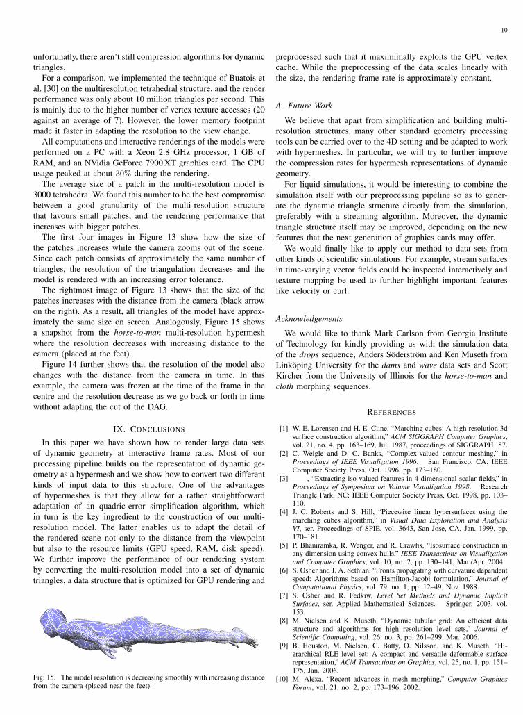
The rightmost image of Figure 13 shows that the size of thepatches increases with the distance from the camera (black arrowon the right). As a result, all triangles of the model have approx-imately the same size on screen. Analogously, Figure 15 showsa snapshot from the horse-to-man multi-resolution hypermeshwhere the resolution decreases with increasing distance to thecamera (placed at the feet).

Figure 14 further shows that the resolution of the model alsochanges with the distance from the camera in time. In thisexample, the camera was frozen at the time of the frame in thecentre and the resolution decrease as we go back or forth in timewithout adapting the cut of the DAG.

IX. CONCLUSIONS

In this paper we have shown how to render large data setsof dynamic geometry at interactive frame rates. Most of ourprocessing pipeline builds on the representation of dynamic ge-ometry as a hypermesh and we show how to convert two differentkinds of input data to this structure. One of the advantagesof hypermeshes is that they allow for a rather straightforwardadaptation of an quadric-error simplification algorithm, whichin turn is the key ingredient to the construction of our multi-resolution model. The latter enables us to adapt the detail ofthe rendered scene not only to the distance from the viewpointbut also to the resource limits (GPU speed, RAM, disk speed).We further improve the performance of our rendering systemby converting the multi-resolution model into a set of dynamictriangles, a data structure that is optimized for GPU rendering and

Fig. 15. The model resolution is decreasing smoothly with increasing distancefrom the camera (placed near the feet).

preprocessed such that it maximimally exploits the GPU vertexcache. While the preprocessing of the data scales linearly withthe size, the rendering frame rate is approximately constant.

A. Future Work

We believe that apart from simplification and building multi-resolution structures, many other standard geometry processingtools can be carried over to the 4D setting and be adapted to workwith hypermeshes. In particular, we will try to further improvethe compression rates for hypermesh representations of dynamicgeometry.

For liquid simulations, it would be interesting to combine thesimulation itself with our preprocessing pipeline so as to gener-ate the dynamic triangle structure directly from the simulation,preferably with a streaming algorithm. Moreover, the dynamictriangle structure itself may be improved, depending on the newfeatures that the next generation of graphics cards may offer.

We would finally like to apply our method to data sets fromother kinds of scientific simulations. For example, stream surfacesin time-varying vector fields could be inspected interactively andtexture mapping be used to further highlight important featureslike velocity or curl.

Acknowledgements

We would like to thank Mark Carlson from Georgia Instituteof Technology for kindly providing us with the simulation dataof the drops sequence, Anders Soderstrom and Ken Museth fromLinkoping University for the dams and wave data sets and ScottKircher from the University of Illinois for the horse-to-man andcloth morphing sequences.

REFERENCES

[1] W. E. Lorensen and H. E. Cline, “Marching cubes: A high resolution 3dsurface construction algorithm,” ACM SIGGRAPH Computer Graphics,vol. 21, no. 4, pp. 163–169, Jul. 1987, proceedings of SIGGRAPH ’87.

[2] C. Weigle and D. C. Banks, “Complex-valued contour meshing,” inProceedings of IEEE Visualization 1996. San Francisco, CA: IEEEComputer Society Press, Oct. 1996, pp. 173–180.

[3] ——, “Extracting iso-valued features in 4-dimensional scalar fields,” inProceedings of Symposium on Volume Visualization 1998. ResearchTriangle Park, NC: IEEE Computer Society Press, Oct. 1998, pp. 103–110.

[4] J. C. Roberts and S. Hill, “Piecewise linear hypersurfaces using themarching cubes algorithm,” in Visual Data Exploration and AnalysisVI, ser. Proceedings of SPIE, vol. 3643, San Jose, CA, Jan. 1999, pp.170–181.

[5] P. Bhaniramka, R. Wenger, and R. Crawfis, “Isosurface construction inany dimension using convex hulls,” IEEE Transactions on Visualizationand Computer Graphics, vol. 10, no. 2, pp. 130–141, Mar./Apr. 2004.

[6] S. Osher and J. A. Sethian, “Fronts propagating with curvature dependentspeed: Algorithms based on Hamilton-Jacobi formulation,” Journal ofComputational Physics, vol. 79, no. 1, pp. 12–49, Nov. 1988.

[7] S. Osher and R. Fedkiw, Level Set Methods and Dynamic ImplicitSurfaces, ser. Applied Mathematical Sciences. Springer, 2003, vol.153.

[8] M. Nielsen and K. Museth, “Dynamic tubular grid: An efficient datastructure and algorithms for high resolution level sets,” Journal ofScientific Computing, vol. 26, no. 3, pp. 261–299, Mar. 2006.

[9] B. Houston, M. Nielsen, C. Batty, O. Nilsson, and K. Museth, “Hi-erarchical RLE level set: A compact and versatile deformable surfacerepresentation,” ACM Transactions on Graphics, vol. 25, no. 1, pp. 151–175, Jan. 2006.

[10] M. Alexa, “Recent advances in mesh morphing,” Computer GraphicsForum, vol. 21, no. 2, pp. 173–196, 2002.

11

[11] N. Anuar and I. Guskov, “Extracting animated meshes with adaptivemotion estimation,” in Proceedings of Vision, Modeling, and Visualiza-tion 2004, B. Girod, M. A. Magnor, and H.-P. Seidel, Eds. Stanford,CA: IOS Press, Nov. 2004, pp. 63–71.

[12] M. Garland and P. S. Heckbert, “Surface simplification using quadricerror metrics,” in Proceedings of SIGGRAPH ’97. Los Angeles, CA:ACM Press, Aug. 1997, pp. 209–216.

[13] M. Garland and Y. Zhou, “Quadric-based simplification in any dimen-sion,” ACM Transactions on Graphics, vol. 24, no. 2, pp. 209–239, Apr.2005.

[14] I. J. Trotts, B. Hamann, K. I. Joy, and D. F. Wiley, “Simplificationof tetrahedral meshes,” in Proceedings of IEEE Visualization 1998.Research Triangle Park, NC: IEEE Computer Society Press, Oct. 1998,pp. 287–295.

[15] H. Vo, S. Callahan, P. Lindstrom, V. Pascucci, and C. Silva, “Streamingsimplification of tetrahedral meshes,” Lawrence Livermore NationalLaboratory, Tech. Rep. UCRL-CONF-208710, Apr. 2005.

[16] P. Cignoni, D. Costanza, C. Montani, C. Rocchini, and R. Scopigno,“Simplification of tetrahedral volume data with accurate error evalua-tion,” in Proceedings IEEE Visualization 2000. IEEE Computer Society,2000, pp. 85–92.

[17] S. Kircher and M. Garland, “Progressive multiresolution meshes for de-forming surfaces,” in Proceedings of Symposium on Computer Animation2005. Los Angeles, CA: ACM Press, Jul. 2005, pp. 191–200.

[18] A. Shamir, V. Pascucci, and C. Bajaj, “Multi-resolution dynamic mesheswith arbitrary deformations,” in Proceedings of IEEE Visualization 2000.Salt Lake City, UT: IEEE Computer Society Press, Oct. 2000, pp. 423–430.

[19] E. Puppo, “Variable resolution triangulations,” Computational Geometry,vol. 11, no. 3–4, pp. 219–238, 1998.

[20] L. D. Floriani, P. Magillo, and E. Puppo, “Efficient implementationof multi-triangulations,” in Proceedings of IEEE Visualization 1998.Research Triangle Park, NC: IEEE Computer Society Press, Oct. 1998,pp. 43–50.

[21] P. Magillo, “Spatial operations on multiresolution cell complexes,” Ph.D.dissertation, Dept. of Computer and Information Sciences, University ofGenova (Italy), 1999.

[22] P. E. P. E. Danovaro, L. De Floriani, “Data structures for 3d multi-tessellations: an overview, in: Data visualization: The state of the art,”Proceedings Dagstuhl Seminar on Scientific Visualization, 2003.

[23] P. Cignoni, L. De Floriani, P. Lindstrom, V. Pascucci, J. Rossignac,and C. Silva, “Multi-resolution modeling, visualization and streamingof volume meshes,” in Eurographics 2004 - Tutorial, 2004.

[24] P. Cignoni, L. De Floriani, P. Magillo, E. Puppo, and R. Scopigno,“Selective refinement queries for volume visualization of unstructuredtetrahedral meshes,” IEEE Transactions on Visualization and ComputerGraphics, vol. 10, no. 1, pp. 29–45, January-February 2004.

[25] P. Cignoni, F. Ganovelli, E. Gobbetti, F. Marton, F. Ponchio, andR. Scopigno, “Batched multi triangulation,” in Proceedings of IEEEVisualization 2005. Minneapolis, MN: IEEE Computer Society Press,Oct. 2005, pp. 207–214.

[26] R. Sondershaus and W. Straßer, “Segment-based tetrahedral meshingand rendering,” in Proceedings of GRAPHITE ’06. Kuala Lumpur,Malaysia: ACM Press, Nov. 2006, pp. 469–477.

[27] V. Pascucci, “Isosurface computation made simple: Hardware acceler-ation, adaptive refinement and tetrahedral stripping,” in Proceedings ofVisSym 2004, O. Deussen, C. Hansen, D. A. Keim, and D. Saupe, Eds.Konstanz, Germany: Eurographics Association, May 2004, pp. 293–300.

[28] T. Klein, S. Stegmaier, and T. Ertl, “Hardware-accelerated reconstructionof polygonal isosurface representations on unstructured grids,” in Pro-ceedings of Pacific Graphics 2004. Seoul, South-Korea: IEEE ComputerSociety Press, Oct. 2004, pp. 186–195.

[29] P. Kipfer and R. Westermann, “GPU construction and transparentrendering of iso-surfaces,” in Proceedings of Vision, Modeling, andVisualization 2005, G. Greiner, J. Hornegger, H. Niemann, and M. Stam-minger, Eds. Erlangen, Germany: IOS Press, Nov. 2005, pp. 241–248.

[30] L. Buatois, G. Caumon, and B. Levy, “GPU accelerated isosurfaceextraction on tetrahedral grids,” in Advances in Visual Computing (ISVC2006), ser. Lecture Notes in Computer Science. Springer, 2006, vol.4291, pp. 383–392.

[31] H.-W. Shen and L.-J. C. K.-L. Ma, “A fast volume rendering algorithmfor time-varying fields using atime-space partitioning (TSP) tree,” inProceedings of IEEE Visualization 1999. San Francisco, CA: IEEEComputer Society Press, Oct. 1999, pp. 371–545.

[32] S. Guthe, M. Wand, J. Gonser, and W. Straßer, “Interactive renderingof large volume data sets,” in Proceedings of IEEE Visualization 2002.Boston, MA: IEEE Computer Society Press, Oct. 2002, pp. 53–60.

[33] C. Wang, J. Gao, L. Li, and H.-W. Shen, “A multiresolution volumerendering framework for large-scale time-varying data visualization,”in Proceedings of Volume Graphics 2005. Stony Brook, NY: IEEEComputer Society Press, Jun. 2005, pp. 11–19.

[34] S.-K. Liao, J. Z. C. La, and Y.-C. Chung, “Time-critical rendering fortime-varying volume data,” Computers & Graphics, vol. 28, no. 2, pp.279–288, Apr. 2004.

[35] M. Strengert, M. Magallon, D. Weiskopf, S. Guthe, and T. Ertl, “Largevolume visualization of compressed time-dependent datasets on GPUclusters,” Parallel Computing, vol. 31, no. 52, pp. 205–219, Feb. 2005.

[36] P. Bhaniramka, R. Wenger, and R. Crawfis, “Isosurfacing in higherdimensions,” in Proceedings of IEEE Visualization 2000. Salt LakeCity, UT: IEEE Computer Society Press, Oct. 2000, pp. 267–273.

[37] S. D. Porumbescu, B. Budge, L. Feng, and K. I. Joy, “Shell maps,”ACM Transactions on Graphics, vol. 24, no. 3, pp. 626–633, Jul. 2005,proceedings of SIGGRAPH 2005.

[38] N. Max, P. Williams, and C. T. Silva, “Approximate volume renderingfor curvilinear and unstructured grids by hardware-assisted polyhedronprojection,” International Journal of Imaging Systems and Technology,vol. 11, pp. 53–61, 2000.

[39] J. Wu and L. Kobbelt, “A stream algorithm for the decimation of massivemeshes,” in Proceedings of Graphics Interface ’03. Halifax, Canada:AK Peters, Jun. 2003, pp. 185–192.

[40] P. Cignoni, F. Ganovelli, E. Gobbetti, F. Marton, F. Ponchio, andR. Scopigno, “Adaptive tetrapuzzles: Efficient out-of-core constructionand visualization of gigantic multiresolution polygonal models,” ACMTransactions on Graphics, vol. 23, no. 3, pp. 796–803, Aug. 2004,proceedings of SIGGRAPH 2004.

[41] S. Lloyd, “Least squares quantization in PCM,” IEEE Transactions onInformation Theory, vol. 28, no. 2, pp. 129–137, 1982.

[42] C.-K. Yang, T. Mitra, and T. cker Chiueh, “On-the-flyrendering of losslessly compressed irregular volume data,” inIEEE Visualization, 2000, pp. 101–108. [Online]. Available:citeseer.ist.psu.edu/yang00fly.html