Ray traced rendering using GPGPU devices

Eastern Washington UniversityEWU Digital Commons

EWU Masters Thesis Collection Student Research and Creative Works

2013

Ray traced rendering using GPGPU devicesCoby SossEastern Washington University

Follow this and additional works at: http://dc.ewu.edu/theses

Part of the Computer Sciences Commons

This Thesis is brought to you for free and open access by the Student Research and Creative Works at EWU Digital Commons. It has been accepted forinclusion in EWU Masters Thesis Collection by an authorized administrator of EWU Digital Commons. For more information, please [email protected].

Recommended CitationSoss, Coby, "Ray traced rendering using GPGPU devices" (2013). EWU Masters Thesis Collection. 101.http://dc.ewu.edu/theses/101

http://dc.ewu.edu?utm_source=dc.ewu.edu%2Ftheses%2F101&utm_medium=PDF&utm_campaign=PDFCoverPages

http://dc.ewu.edu/theses?utm_source=dc.ewu.edu%2Ftheses%2F101&utm_medium=PDF&utm_campaign=PDFCoverPages

http://dc.ewu.edu/student_research?utm_source=dc.ewu.edu%2Ftheses%2F101&utm_medium=PDF&utm_campaign=PDFCoverPages

http://dc.ewu.edu/theses?utm_source=dc.ewu.edu%2Ftheses%2F101&utm_medium=PDF&utm_campaign=PDFCoverPages

http://network.bepress.com/hgg/discipline/142?utm_source=dc.ewu.edu%2Ftheses%2F101&utm_medium=PDF&utm_campaign=PDFCoverPages

http://dc.ewu.edu/theses/101?utm_source=dc.ewu.edu%2Ftheses%2F101&utm_medium=PDF&utm_campaign=PDFCoverPages

mailto:[email protected]

Ray Traced Rendering Using GPGPU Devices

A Thesis

Presented To

Eastern Washington University

Cheney, Washington

In Partial Fulfillment of the Requirements

for the Degree

Master of Science in Computer Science

By

Coby Soss

Spring 2013

THESIS OF Coby Soss APPROVED BY

DATE

Dr. Paul Schimpf, GRADUATE STUDY COMMITTEE

DATE

Dr. Bill Clark, GRADUATE STUDY COMMITTEE

MASTER’S THESIS

In presenting this thesis in partial fulfillment of the requirements for a master’s degree

at Eastern Washington University, I agree that the JFK Library shall make copies freely

available for inspection. I further agree that copying of this project in whole or in part is

allowable only for scholarly purposes. It is understood, however, that any copying or

publication of this thesis for commercial purposes, or for financial gain, shall not be

allowed without my written permission.

Signature

Date

iv

ABSTRACT

Ray tracing is a very popular way to draw 3-D scenes onto a 2-D image. The technique produces a very

high degree of visual realism with regard to shadows, reflection, and refraction. The drawback of this

technique is the fact that it is extremely computationally expensive. This expense has been a barrier to

using ray tracing to implement real-time rendering. Recent technological advances have fueled increased

interest in the technique because the prospect of real-time ray tracing in commercial applications is now

closer to becoming a reality. This thesis is an attempt to quantify the degree of speed-up, in terms of raw

processing power, that this new class of GPU hardware makes possible.

v

ACKNOWLEDGEMENTS

I would like to thank Dr. Bill Clark for content direction as well as editing suggestions, along with Dr. Paul

Schimpf for providing suggestions related to graphics hardware. Mike Henry also contributed to the

editing of this document. Lastly, I would like to thank the team efforts of those at the EWU Computer

Science department who made my masters journey flow smoothly. You know who you are.

vi

Abstract .......................................................................................................................................................... iv

Acknowledgements ........................................................................................................................................ v

1 Introduction ........................................................................................................................................... 1

2 Related Work ......................................................................................................................................... 2

3 Ray Tracing Fundamentals ..................................................................................................................... 2

3.1 Rendering ...................................................................................................................................... 2

3.2 Ray Tracing .................................................................................................................................... 3

3.3 Forward Ray Tracing...................................................................................................................... 4

3.4 Backward Ray Tracing ................................................................................................................... 4

3.5 Ray Generation .............................................................................................................................. 4

3.6 Ray Tracing Algorithm ................................................................................................................... 7

4 Algorithm Mathematics ....................................................................................................................... 10

4.1 Intersection Calculations............................................................................................................. 10

4.1.1 Sphere Intersection ................................................................................................................. 10

4.1.2 Sphere Surface Normal Vector ............................................................................................... 12

4.1.3 Triangle Intersection ............................................................................................................... 12

4.1.4 Triangle Surface Normal Vector ............................................................................................. 13

4.2 Phong Shading Model ................................................................................................................. 15

4.3 Phong Illumination ...................................................................................................................... 15

4.3.1 Diffuse Reflection.................................................................................................................... 16

4.3.2 Specular Reflection ................................................................................................................. 16

4.3.3 Ambient Reflection ................................................................................................................. 17

4.3.4 Calculating Pixel Color Intensities .......................................................................................... 17

4.4 Reflection Calculation ................................................................................................................. 18

5 Parallelizing the Algorithm .................................................................................................................. 20

5.1 Stream Processing ....................................................................................................................... 21

5.1.1 SPMD and SIMD Data Parallelism .......................................................................................... 21

5.1.2 Parallelism in the Ray Tracer .................................................................................................. 21

5.2 Overview of OpenCL.................................................................................................................... 22

vii

5.2.1 OpenCL Memory Model.......................................................................................................... 22

5.2.2 OpenCL Execution Model ....................................................................................................... 23

5.2.3 Executing a Kernel In JOCL ...................................................................................................... 25

5.2.4 OpenCL Issues ......................................................................................................................... 28

5.3 Implementing PS-Triangle in an SPMD Kernel ........................................................................... 28

5.3.1 Algorithm Design .................................................................................................................... 29

5.3.2 Data Structure Mapping for the Triangle Intersection Kernel ............................................... 30

5.3.3 Caching Triangle Data Structures ........................................................................................... 32

5.4 Implementing PS-Ray in an SPMD Kernel .................................................................................. 32

5.4.1 Algorithm Design .................................................................................................................... 32

6 AMD Radeon Mobility 5870 GPU ........................................................................................................ 36

6.1 Hardware Specifications ............................................................................................................. 36

6.2 Memory Considerations .............................................................................................................. 36

6.3 Mapping the Radeon Mobility 5870 to the OpenCL Memory Model ........................................ 36

7 Results .................................................................................................................................................. 37

7.1 Single-threaded Triangle Intersection ........................................................................................ 40

7.2 Parallel Strategies versus Single-threaded Triangle Intersection .............................................. 41

8 Future Work ......................................................................................................................................... 41

9 Conclusions .......................................................................................................................................... 41

Figure 1 - Foundational ray tracing concepts .................................................................................................. 3

Figure 2 - Mapping a hypothetical 6 pixel monitor to 30x20 image plane ...................................................... 7

Figure 3 - Shadow rays .................................................................................................................................... 9

Figure 4 – Reflection ........................................................................................................................................ 9

Figure 5 - Relationship between vertex normals and barycentric coordinates u and v ................................ 14

Figure 6 - Gouraud shading (Left) vs Ray traced Phong shading (Middle) along with underlying geometry

(Right) ............................................................................................................................................................ 15

Figure 7 - Mathematics of relection .............................................................................................................. 20

Figure 8 - Opencl memory model .................................................................................................................. 22

Figure 9 - Triangle intersection parallelization .............................................................................................. 30

Figure 10 - Ray Data Format .......................................................................................................................... 31

Figure 11 - Triangle data for the triangle intersection kernel ....................................................................... 31

Figure 12 - Triangle intersection output stream ........................................................................................... 31

Figure 13 - Ray trace parallelization .............................................................................................................. 33

Figure 14 - Ray data layout for ray trace kernel ............................................................................................ 34

Figure 15 - Sphere data layout ...................................................................................................................... 35

Figure 16 - Triangle data layout ..................................................................................................................... 35

Figure 17 - Pixel output stream format ......................................................................................................... 35

viii

Figure 18 - Mapping AMD Radeon hardware to the OpenCL memory model .............................................. 37

Figure 19 - Reflections on teapot for both handles and the spout ............................................................... 38

Figure 20 - Comparing timings of PS-Ray and PS-Triangle to single-threaded triangle intersection ............ 39

1 INTRODUCTION

The first commercially available personal computer system to have a separate graphics processor apart

from the CPU was the revolutionary Commodore Amiga. Since that time, the ever increasing popularity of

video games, combined with market pressure for more realistic looking graphics, has driven the creation

of very advanced graphics hardware that can perform faster than a CPU in many parallel computation

tasks. The graphics card company NVidia was the first company to use the term Graphics Processing Unit,

or GPU, as an acknowledgment that graphics cards had evolved into massively parallel computers that run

alongside the main system CPU(s).

Traditionally, a GPU is a processor that is designed to perform the rapid execution of the traditional fixed

graphics pipeline. The phrase “fixed graphics pipeline” refers to a graphics programming paradigm in

which many operations that the graphics card executes are not alterable (programmable) by the

programmer [16]. Rapid advances in GPUs have allowed more custom programmability of the GPU

hardware as well as the addition of floating point capabilities in 2003 [12]. As a consequence, the fixed

graphics pipeline has been superseded by user-programmable pipelines in which the API allows users to

write code for parts of the pipeline known as shaders [30]. These APIs do a better job of utilizing the full

computing power of this programmable graphics hardware. This has allowed for the computational power

of the graphics card to be used in new ways. For instance, it is now possible to leverage the GPU to

perform general-purpose parallel computation tasks that do not necessarily have anything to do with any

graphics pipeline [14], [8].

Additionally, parallel computation has received increased attention due to the current limitations that

have been encountered with attempts to increase the speed of single-core CPUs, namely the ability to

dissipate heat quickly enough [15], [5]. Newer CPUs have achieved greater processing power while

avoiding heat problems by increasing the number of processor cores instead of increasing the processor’s

frequency.

OpenCL is an API that has been written to utilize multicore processors of all types, including GPUs, to

facilitate parallel processing in a heterogeneous processor environment. It allows a programmer to

develop code in an ANSI C99-based language which can be compiled for multiple different processor

architectures [17], [22], [23]. This is another way of saying that OpenCL code that is written against one

type of GPU should run against another with little or no modification of code. By comparison, earlier GPU

programming languages suffer from portability issues and require extensive practice to master [10], [14],

[6], [25]. This thesis describes the process of implementing a ray tracing [1] algorithm in OpenCL, utilizing

a Radeon Mobility 5870 GPU as the computation device.

2

2 RELATED WORK

There is a large amount of research directed toward the problem of increasing the speed of ray tracing

through various parallelization attempts in GPU hardware [19], [9] as well as in other types of hardware

[20]. These research activities have helped to motivate the current interest level in GPGPU technology.

Some papers have alluded to the fact that OpenCL’s cross-platform capabilities come at the cost of some

performance [12], [15]. In other words, multiple research projects have reaffirmed what the Computer

Science community has learned from experience – these early attempts at cross-platform technology

often result in a performance loss when compared to custom low-level implementations [7]. However,

this should not detract from the importance of the exercise of developing and using cross-platform

technology that works seamlessly across different hardware platforms. The benefits have been shown to

outweigh the cost in most development scenarios.

3 RAY TRACING FUNDAMENTALS

The sections that follow provide the necessary background on ray tracing so that one can better

understand the results of this project.

3.1 RENDERING

In computer graphics, the process of drawing 3-D geometry to a 2-D screen image in such a way that it

appears 3-D with appropriate colors is called rendering. There is more than one way to achieve this effect.

One very popular technique is called ray tracing, which is the technique used in this project. The reason

for ray tracing’s popularity stems from the fact that the algorithm’s recursive nature makes it simple to

implement. The technique also provides very accurate reflections, shadows, and refraction to a degree

that is above and beyond what other rendering methods provide. Before a more in-depth discussion of

ray tracing, it is necessary to define a few terms:

Image plane – The mathematical plane on which the ray-traced image will be drawn.

View frustrum – The 3-D volume in space that includes all visible objects which will be projected onto the

image plane during rendering.

Pixel – Abbreviated term for picture element. It is the smallest addressable region of 2-D space on a

computer monitor. Each pixel is represented in the frame buffer by a 32-bit integer (in most present-day

scenarios).

Frame buffer – A memory location, usually on the graphics card, where color data used to set pixel colors

is stored, usually in the form of a large array of 32-bit integers. For each 32-bit integer in the frame

3

buffer, the first 8 bits represent the red component of a color, the second 8 bits represent the green

component of the color, and the third 8 bits represent the blue component of the color. The final 8 bits

are used for purposes that are outside the scope of this project.

It may be worthwhile to note that, conceptually, ray tracing is very similar to the behavior of light in a

pinhole camera [26]. In the case of a pinhole camera, light enters a hole in an otherwise light-proof box

and strikes film on the back of the box. This process of photons hitting this film creates an image of what

is in front of the pinhole. The image plane is comparable to the pinhole camera film. The camera is

comparable to the pinhole. A key difference between the image plane and the pinhole camera film is that

the image plane is in front of the camera instead of behind it, resulting in an image that is not inverted

[26]. In contrast, the camera film is behind the pinhole, which inverts the image on the film. Figure 1

shows the comparison of a pinhole camera to ray tracing concepts.

FIGURE 1 - FOUNDATIONAL RAY TRACING CONCEPTS

3.2 RAY TRACING

Imagine a room with a single source of light and multiple objects in it. The light source will emit photons,

and each photon will travel on a path known as a light ray. These photons will strike objects and re-emit

from the surface of those struck objects. Each such interaction is essentially a “reflection”. In this way,

photons will bounce around the entire scene until they run out of energy. Objects can be directly lit by a

light source or indirectly lit from a reflection off of another object. Let’s say that there is a camera in the

scene oriented in space. Some photons will enter the camera lens, and some photons will not. The

4

photons that enter the camera lens contribute to the image seen by the camera. Determining the path

that a photon takes as it travels around a scene is what is known as ray tracing [26].

3.3 FORWARD RAY TRACING

Forward ray tracing is a particular kind of ray tracing that follows the path that photons take from their

light source. The “forward” aspect of this naming refers to the fact that we are keeping track of the path

photons take on their journey from their light source as they enter the room. This is an accurate but

wasteful approach because photons that do not enter the camera lens do not contribute to the

constructed image. The sheer number of photons that do not reach the camera lens but need to be traced

results in an extremely time-consuming algorithm [26].

3.4 BACKWARD RAY TRACING

The solution to this wastefulness is to only consider the photons that contribute to the image (i.e., enter

the camera lens). We do this by reversing the ray tracing problem and trace photon paths starting from

the camera, moving backward into the scene. The process of backward ray tracing begins with the

assumption that all photons that strike the image plane will be photons that contribute to the image. A

convenient way to model this reverse light ray is with the mathematical concept of a ray, which has both

a starting point and a direction. To calculate the color of every pixel on the screen, we extend a ray

through every pixel-sized portion of the image plane and use the ray tracing algorithm to retrieve the

color for that pixel [26]. The ray is mathematically defined below.

Ray – A ray is mathematical line used the model the path of light rays in a 3-D volume. It is expressed

parametrically as R�t� � O � t where:

R�t� represents the ray.

O represents the ray origin point.

represents the normalized ray direction vector.

t represents a scalar multiplier(parameter) that determines a particular location on the ray. It has

a valid range of �, ∞�. 3.5 RAY GENERATION

The process of determining the x-y coordinates through which to extend a ray is a matter of finding the

pixel center for each considered pixel on the image plane. This process is a substantial part of ray

generation. In order to best explain how to generate rays, it is useful to consider a simplified scenario that

5

uses a fictitious monitor resolution of 6 pixels. We will map the image plane onto these 6 pixels to show

how it is done; a real screen resolution has many more pixels, of course.

A fast way of determining the center of a pixel is to calculate the pixel’s width and height on the image

plane.

In order to calculate these two values, we need the image plane dimensions and the monitor resolution

dimensions. Let’s say that the image plane X dimension (width) is [-15, 15] in world coordinates and the

image plane Y dimension (height) is [-10, 10] in world coordinates. The screen resolution dimensions are 3

pixels by 2 pixels, comprising our 6-pixel monitor resolution.

��

� �� units in world coordinates

��

� �� units in world coordinates

Now that these values are calculated, it is clear that a pixel is 10x10 units on our image plane. With this

information and the lower-left coordinates of the image plane, we can calculate the x-y location of the

first pixel on the image plane. Since it is most accurate to have the ray pierce the center of each 10x10

square on the image plane that represents a pixel, we add 5 to each dimension(x and y) of the lower-left

coordinate of the image plane. In doing so, the ray pierces the center of the first pixel instead of the

lower-left corner of the first pixel.

The step-by-step process for determining the x-y coordinates for each pixel will now be explained in

detail. We start with:

Left-most X = -15

Bottom-most Y = Image plane bottom = -10

Adjust left-most X and bottom-most Y so that they are centered in the image plane area correspoding to

the first pixel.

Current pixel X = Left-most X + 5

Current pixel Y = Bottom-most Y + 5

Now we are in the center of the first pixel.

6

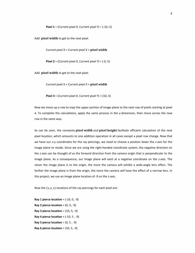
Pixel 1 = (Current pixel X, Current pixel Y) = (-10,-5)

Add �� to get to the next pixel.

Current pixel X = Current pixel X + ��

Pixel 2 = (Current pixel X, Current pixel Y) = ( 0,-5)

Add �� to get to the next pixel.

Current pixel X = Current pixel X + ��

Pixel 3 = (Current pixel X, Current pixel Y) = (10,-5)

Now we move up a row to map the upper portion of image plane to the next row of pixels starting at pixel

4. To complete the calculations, apply the same process in the y-dimension, then move across the new

row in the same way.

As can be seen, the constants �� and �� facilitate efficient calculation of the next

pixel location, which amounts to one addition operation in all cases except a pixel row change. Now that

we have our x-y coordinates for the ray piercings, we need to choose a position down the z-axis for the

image plane to reside. Since we are using the right-handed coordinate system, the negative direction on

the z-axis can be thought of as the forward direction from the camera origin that is perpendicular to the

image plane. As a consequence, our image plane will exist at a negative coordinate on the z-axis. The

closer the image plane is to the origin, the more the camera will exhibit a wide-angle lens effect. The

farther the image plane is from the origin, the more the camera will have the effect of a narrow lens. In

this project, we use an image plane location of -9 on the z-axis.

Now the �x, y, z� locations of the ray piercings for each pixel are:

Ray 1 pierce location = (-10,-5, -9)

Ray 2 pierce location = (0,-5, -9)

Ray 3 pierce location = (10,-5, -9)

Ray 4 pierce location = (-10, 5 , -9)

Ray 5 pierce location = (0, 5 , -9)

Ray 6 pierce location = (10, 5, -9)

7

Next, we need to calculate the rays. For each ray, we start with the origin at �0, 0, 0� and use its ray pierce

location and the origin to calculate its vector, which is then normalized. Once we have the parametric

ray equation for all six rays, we can use these rays to ray trace. The image plane of Figure 2 shows the X

and Y locations on the plane where each of the 6 rays will pierce the plane, represented as dots. The left

portion of the figure shows the corresponding pixels and the order in which they are mapped to the

image plane. While a 6-pixel resolution is highly unlikely in real-world instances, this algorithm is

applicable to a screen resolution of any number of pixels and to any image plane(window) size.

FIGURE 2 - MAPPING A HYPOTHETICAL 6 PIXEL MONITOR TO 30X20 IMAGE PLANE

3.6 RAY TRACING ALGORITHM

Before discussing the ray tracing algorithm, it is necessary to define some terms:

Polygonal mesh - A polygonal mesh is a collection of vertices, edges, and faces that defines the shape of a

3-D object in 3-D computer graphics.

Bounding sphere - A bounding sphere is the smallest enclosing sphere that surrounds each polygonal

mesh in the scene. It is used to accelerate intersection testing with the bounded polygonal object.

The ray tracing algorithm is as follows:

For each pixel on the screen:

0) Calculate a primary ray that originates at the virtual camera lens and goes through

the location on the image plane associated with the center of the current pixel. This

is the process that was covered in the previous section.

8

1) For each bounding sphere, determine whether a ray intersects with the sphere.

a. If the ray intersects the current sphere, intersection tests need to be

performed against all triangles inside the bounding sphere.

i. If an intersection with a triangle has occurred and it is the closest

found so far, record it as the closest.

b. If the ray does not intersect the current sphere, go to the next sphere in

the list and proceed to step 1a.

2) If the ray did not intersect any triangles, set the current pixel to the background

color, go to the next pixel and return to step 0, otherwise continue to step 3.

3) Determine the shade (color) at the intersection point of the ray with the triangle.

This process is known as shading. The steps for shading are as follows:

a. Obtain a color value using the Phong Illumination Model of Section 4.3.

b. When calculating a shade value at an intersection point, do not include

lighting contributions from any light which is obstructed by another object.

In order to determine whether an intersection point is shadowed, we need

to determine whether any light sources contributing to the shade value of

that location are obstructed by another object. To accomplish this, we cast

a shadow ray from the intersection point to each light source. We then

apply our sphere and triangle intersection routine to each ray in order to

determine whether the ray intersects with another object on its way to the

light source. If any ray intersects with an object, we know that the

particular light source we are testing is obstructed by the intersected

object. Each obstructed light source does not contribute to the shade value

at the intersection point. Figure 3 shows an example of an obstructed light

source and an unobstructed light source.

9

FIGURE 3 - SHADOW RAYS

c. Obtain color contributions from reflections. Once a ray actually hits a

surface, there will be a reflected ray. This ray may or may not strike

another object. If the reflected ray does strike another object, the color of

the struck object at the point it is intersected by the ray will be added to

the color of the original intersection point as a percentage contribution to

that intersection point’s color. In the unmodified ray trace algorithm, this

reflection process is recursive. In this project, however, the reflection is

limited to one reflected ray per primary ray because OpenCL kernels do

not allow recursion and the iterative version of this algorithm is very

complex.

FIGURE 4 – REFLECTION

10

4) If the current pixel is the last pixel, terminate the algorithm, otherwise go to the

next pixel and return to step 0.

4 ALGORITHM MATHEMATICS

The mathematical operations for the ray tracing algorithm are visited in the sections that follow.

4.1 INTERSECTION CALCULATIONS

The following sections detail the first major step of the ray tracing algorithm – finding the closest point at

which the ray intersects with an object.

4.1.1 SPHERE INTERSECTION

In terms of computational time, trying to intersect a ray with a list of triangles that comprise an object

takes much longer than intersecting with a single bounding sphere. For example, if an object is

constructed using 40,000 triangles, we would need to attempt to intersect with all of the triangles to

determine which triangles, if any, have been intersected. For this reason, an optimization step that

involves first intersecting with a bounding sphere is desirable. Intersecting with a bounding sphere is

much less costly than intersecting with a triangle and is only a single intersection calculation. In contrast,

in the absence of bounding spheres, we would need to perform intersection calculations with all triangles

in the scene. Unless the number of triangles comprising our scene’s objects is very small, this will result in

many expensive triangle intersection calculations for triangles that are nowhere near the ray we are

testing. If the ray does not intersect with any of the triangles, all the computation that has been

attempted is wasteful.

Below are the calculations for performing ray intersection with a sphere:

The ray R�t� with origin point O and direction vector can be written parametrically as:

R�t� � O � t t & 0 �1�

The function R�t� represents a point on the ray for any specific value of t.

� �(��) , *��), +��)� �2�

X./01 � Y./01 � Z./01 � 1 �3� This is true because the direction vector is a normalized

vector.

The equation for the sphere is:

11

Sphere radius: S0 �4�

Sphere Center: S789:80 � �X7, Y7, Z7� �5�

A point on the surface of the sphere �X<, Y<, Z<� is given by:

�X< = X7�1 � �Y< = Y7�1 � �Z< = Z7�1 � S01 �6�

Since the intersection point on the sphere is also a point on the ray we can rewrite the ray equation to

express a candidate sphere surface point in terms of the ray:

X � X? � X./0 @ t �7�

Y � Y? � Y./0 @ t Z � Z? � Z./0 @ t

We now substitute these equations for �X<, Y<, Z<� in equation �6�. We solve for t to test whether the

point is on the sphere.

�X? � X./0 @ t = X7�1 � �Y? � Y./0 @ t = Y7�1 � �Z? � Z./0 @ t = Z7�1 � S01 �8�

Equation �8� can be written as a quadratic equation in t as:

A @ t1 � B @ t � C � 0 �9�

The coefficients A, B, and C are in terms of the sphere and the ray and can be computed:

A � X./01 � Y./01 � Z./01 � 1 �10�

B � 2 @ �X./0 @ �X? = X7� � Y./0 @ �Y? = Y7� � Z./0 @ �Z? = Z7� �

C � �X? = X7�1 � �Y? = Y7�1 � �Z? = Z7�1 Solving �G� using the quadratic formula, with A � 1:

tH � �I� J�IK�L@M�1 �11�

tN � �IO J�IK�L@M�1

If B1 = 4 @ C P 0, the ray does not intersect the sphere because there are no real roots and hence no

solution that can be used in the ray equation. This essentially means that the ray does not intersect the

sphere.

12

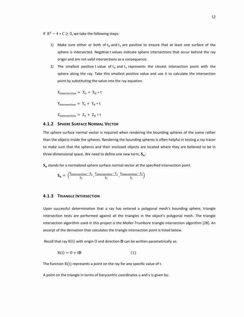
If B1 = 4 @ C Q 0, we take the following steps:

1) Make sure either or both of tH and tN are positive to ensure that at least one surface of the

sphere is intersected. Negative t values indicate sphere intersections that occur behind the ray

origin and are not valid intersections as a consequence.

2) The smallest positive t value of tH and tN represents the closest intersection point with the

sphere along the ray. Take this smallest positive value and use it to calculate the intersection

point by substituting the value into the ray equation.

X/9:80<87:/?9 � X? � X. @ t

Y/9:80<87:/?9 � Y? � Y. @ t Z/9:80<87:/?9 � Z? � Z. @ t

4.1.2 SPHERE SURFACE NORMAL VECTOR

The sphere surface normal vector is required when rendering the bounding spheres of the scene rather

than the objects inside the spheres. Rendering the bounding spheres is often helpful in testing a ray tracer

to make sure that the spheres and their enclosed objects are located where they are believed to be in

three-dimensional space. We need to define one new term, RS:

RS stands for a normalized sphere surface normal vector at the specified intersection point.

RS � TUVWXYZ[Y\XV]W� U\^Z , _VWXYZ[Y\XV]W� _\

^Z , `VWXYZ[Y\XV]W� `\^Z a

4.1.3 TRIANGLE INTERSECTION

Upon successful determination that a ray has entered a polygonal mesh’s bounding sphere, triangle

intersection tests are performed against all the triangles in the object’s polygonal mesh. The triangle

intersection algorithm used in this project is the Moller-Trumbore triangle intersection algorithm [28]. An

excerpt of the derivation that calculates the triangle intersection point is listed below.

Recall that ray R�t� with origin O and direction can be written parametrically as:

R�t� � O � t �1�

The function R�t� represents a point on the ray for any specific value of t.

A point on the triangle in terms of barycentric coordinates u and v is given by:

13

T�u, v� � �1 = u = v�VH � uVN � vV1 �2�

Given the above, the ray will intersect with the triangle when R�t� � T�u, v�. So we would like to find out

what values of t, u, and v, if any, make that equality true.

Substituting:

O � t � �1 = u = v�VH � uVN � vV1 �3�

Rearranging terms and expressing the left side in matrix form yields:

=, VN = VH, V1 = VHf g tuvh � O = VH �4�

If we let M � =, VN = VH, V1 = VHf then the algebraic solution to �4� can be written as:

M�NM g tuvh � M�N�O = VH� �5�

Since M�NM is just the identity matrix, we are left with:

g tuvh � M�N�O = VH� �6�

Using Cramer’s rule and some linear algebra rules, it can be shown that the solution in terms of triangle

vertices and the ray components is:

g tuvh � M�N�O = VH� � 1j x �V1 = VH�k . �VN = VH� lm

mnj�O = VH�x �VN = VH�k . �V1 = VH�

j x �V1 = VH�k . �O = VH��O = VH�x�VN = VH�� . op

pq �7�

The triangle is intersected by the ray if 0 r u r 1,0 r v r 1, u � v r 1. Otherwise, the ray missed the

triangle. If the ray does hit the triangle, t is used in the ray equation to calculate the intersection point.

The u and v parameters are used to interpolate the normal that will be used when we discuss the Phong

Shading Model.

4.1.4 TRIANGLE SURFACE NORMAL VECTOR

Calculating the triangle surface normal vector at a particular intersection point is more involved than

calculating the surface normal vector of the sphere. There is one normal vector associated with each

triangle vertex. We must interpolate the intersection point’s normal vector from all three of these vertex

normal vectors. The interpolation is performed using the u and v values obtained from the triangle

intersection step of the previous section. As Figure 5 shows, u, v and 1 = u = v represent the distances of

14

any point on the triangle from its vertices. Since they can be viewed as weighting values, they are also

used to interpolate vertex normal vectors, vertex color, and vertex texture coordinates. The interpolation

of the surface normal vector at the intersection point is as follows:

Let us call the three normal vectors associated with the triangle vertices s�, s�, s�. Then the triangle normal vector at the intersection point is:

tS� � �1 = u = v�s�� jus��k � �vs��

tSu � �1 = u = v�s�u � Tus�ua � �vs�u�

tSv � �1 = u = v�s�� jws��k � �xs��

FIGURE 5 - RELATIONSHIP BETWEEN VERTEX NORMALS AND BARYCENTRIC COORDINATES U AND V

Normalize:

Ty89z:{ � |tS�� tSu

� � tSv�

tS� � tS�}~YW�X�

tSu � tSu}~YW�X�

tSv � tSv}~YW�X�

15

4.2 PHONG SHADING MODEL

There are multiple approaches to shading. One of the earlier approaches is known as Gouraud shading. It

is calculated by interpolating vertex color across a polygon. The left-most monkey head in Figure 6 shows

the gradual brightness gradient produced by Gouraud shading, particularly with respect to the monkey’s

nose area.

In contrast, the Phong shading model requires that a separate shade value be calculated at each point on

a triangle’s surface. Thus, the normal vector at each point in a triangle is a weighted sum of the normal

vectors at the triangle’s vertices. Each of these calculated normal vectors are then used to calculate a

separate shade. The middle monkey head of Figure 6 shows an example of Phong shading. The net effect

of recalculating a shade value at each intersection point is that the drop-off in brightness starting from the

center of the monkey’s nose is much more pronounced in Phong shading than it is for the vertex color

interpolation of Gouraud shading – meaning shininess is more obvious.

FIGURE 6 - GOURAUD SHADING (LEFT) VS RAY TRACED PHONG SHADING (MIDDLE) ALONG WITH UNDERLYING GEOMETRY

(RIGHT)

4.3 PHONG ILLUMINATION

Phong Illumination attempts to model the way light interacts with a surface. Its calculations are

performed using the normal vector obtained from the calculations of the Phong shading model. Within

the Phong illumination model, there are two categories of properties that generate the color at an

intersection point: light properties and material properties. Light reflected from a surface is arbitrarily

broken down into three components: diffuse, specular, and ambient. These reflections will be discussed in

the following sections but some definitions are first necessary.

Reflection coefficient – A reflection coefficient is a way to model the degree to which a particular

material reflects or absorbs light of different wavelengths. Thus, reflection coefficients determine the

color of the reflection. The range of this value is 0,1f and is multiplied by the corresponding light

property’s value. These coefficients effectively act as scaling values for light intensities.

16

Light Intensity – A light intensity in the Phong Illumination Model captures the color and brightness of the

specular, diffuse, or ambient component of a light source. The model allows for the color of each of these

components to be different but in physical reality the colors of each of these components are the same.

It is worthwhile to note that although these categorizations of light produce realistic looking results in the

Phong illumination model, they are not an accurate portrayal of the way light behaves in nature. In

reality, light has a color determined by an energy level. Certain materials reflect some colors better

than others and the effects of this will be seen in the reflected color. This physical behavior is what

the “material color”, expressed using K<, K., and K�, is modeling [26].

4.3.1 DIFFUSE REFLECTION

Diffuse light is reflected in all directions and originates from active light sources. The theoretical

foundation for the diffuse reflection calculation is Lambert’s Law. This law states that the cosine of the

angle between the normal vector s of the surface intersection point on the polygon and the normalized

light vector �� extending from the intersection point to the light source ls is directly proportional to

the brightness of the diffuse reflection. Therefore, the total diffuse contribution of the shade value at a

given intersection point is determined by adding up the diffuse reflections from all light sources using

Lambert’s Law. The cosine of the angle between any two normalized vectors is the dot product of those

vectors. For any given light source, we take the dot product of the normalized light vector and the

intersection point’s surface normal vector to calculate the cosine of the angle between them. We then

take the resultant value and multiply it by the material’s diffuse reflection coefficient K. and the light’s

diffuse intensity Iy<,.. Remember that the dot product, or cosine, between two normalized vectors is

closer to 0 if the angle between the vectors is near 90 degrees. The dot product is closer to 1 if the angle

between the normalized vectors is small. In other words, when the normalized light vector and the

normal vector are closer, the diffuse reflection will be more intense. It is important to note that the

diffuse reflection does not depend on the view direction, and the reflection is most intense along the

normal vector. The view direction is not included in the calculation because the diffuse reflection scatters

in all directions. The diffuse term is defined below.

K. �� . s�Iy<,.

4.3.2 SPECULAR REFLECTION

Specular light is caused by mirror-like reflections off a smooth surface. This type of light results in shiny

spots on objects. The specular reflection was developed by Bui Tuong Phong [32]. Like the diffuse

contribution, the total specular reflection of the shade value is determined by adding up the specular

contributions from all light sources. The normalized reflection vector �� results from the light source

ls reflecting off the intersection point about the normal vector s. The specular reflection is

17

maximized when the normalized view vector � which points from the intersection point toward the

viewpoint and the normalized reflection vector �� are aligned, and it drops off when � is not near ��.

That is, it is another calculation that involves determining the cosine of the angle between two vectors in

order to derive light intensity. As a consequence, we take the dot product of the intersection point’s

reflection vector and the view vector.

α is a shininess constant for the material. Material shininess captures where on the spectrum of

shininess the material falls. Its value models the smoothness of a surface ranging from very coarse to

very smooth. A smoother surface corresponds to a more perfectly reflective surface and a smaller

specular highlight (shiny spot). A coarser surface corresponds to a less perfectly reflective surface

and has larger specular highlights as a result, since light scatters in many directions. The dot product

calculation is raised to this shininess constant. Next, the specular reflection coefficient K< and

specular light intensity Iy<,< are both multiplied into the current equation as shown below.

K< �� . �� Iy<,<

4.3.3 AMBIENT REFLECTION

Ambient light is light whose source cannot be determined easily. It is intended to model scattered

environmental light and can thought of as a sort of “brightness adjustment”. Ambient reflection is

calculated by multiplying the ambient light intensity I� by the material’s ambient reflection coefficient K�.

It is constant for each material and light combination and is calculated as follows:

K�I�

Each location that needs color shading will have some percentage contribution from each of these

components. The color value from ambient reflection is determined by the material type of a surface and

is not affected by the surface normal vector or the view direction.

4.3.4 CALCULATING PIXEL COLOR INTENSITIES

The Phong illumination model can be summarized with the following set of equations,

componentized by color and obtained by adding up all the previously discussed contributions. The

subscripts on a, s, and d(ambient, diffuse, and specular) denote a color component r, g or b (red, green, or

blue) pertaining to the associated variable.

LS is the set of all light sources that are shining on the objects in the scene. The color values for a

given pixel will likely be altered by the combined effect of all the light sources interacting with, and

reflecting from, surfaces.

I�Z represents the shade value of the red component of the pixel color in RGB format.

18

I�� represents the shade value of the green component of the pixel color in RGB format.

I�� represents the shade value of the blue component of the pixel color in RGB format.

I�Z = K�ZI�Z + ∑ �K.Z �� . s�Iy<,.Z � K<Z �� . �� Iy<,<Z�y< ��^

Clamp I�Z to the range [0, 1].

I�� = K��I�� + ∑ �K.� �� . s�Iy<,.� � K<� �� . �� Iy<,<��y< ��^

Clamp �� to the range [0, 1].

I�� = K��I�� + ∑ �K.� �� . s�Iy<,.� � K<� �� . �� Iy<,<��y< ��^

Clamp �� to the range [0, 1].

Finally, the pixel color is obtained by converting the above values into values compatible with a 24-bit RGB

format. How this process is done depends on the drawing API being used.

4.4 REFLECTION CALCULATION

The description of ray reflection can be expressed using the following terms:

s - The normalized surface normal vector.

� - The normalized incident light vector.

� - The normalized reflected light vector.

��- The component of � perpendicular to the intersected surface.

�� - The component of � parallel to the intersected surface.

�� - The component of � perpendicular to the intersected surface.

�� - The component of � parallel to the intersected surface.

�� - The angle that the incident light ray strikes the surface.

�) - The angle that the incident light ray reflects from the surface.

19

With these values, we can calculate the reflected ray � as follows:

First we note that

�� ).

It follows from this that:

��S� �� S� �) � ��

��S �� S �) ��

�� -��

�� is obtained by projecting � onto s (see Figure 7).

The formula to project � onto a normal s is given by:

�� .s|s|� s ��

Since s is normalized (in other words, it has a length of 1) this equation simply becomes ��:

�� . s��s� ��

� � ��

Using equations ��, �� and �� we can derive � � from ��.

� � �� =��

� � �� = �� =�� ¡�

� � � = �� ¢�

Using equation��, we can rewrite �¢� as

� � � = �j��. s��s�k �G�

The appeal of the equation as it exists in form �G� is that it can be used with the vectors that we have

already computed at the reflection stage of the ray trace algorithm.

20

FIGURE 7 - MATHEMATICS OF RELECTION

5 PARALLELIZING THE ALGORITHM

Parallelizing a sequential algorithm involves analyzing the algorithm for code locations that can be

processed in parallel. Many algorithms have more than one location that can be parallelized. In the case

of the ray tracing algorithm, there are two locations within the algorithm that can be parallelized [18]. The

first parallelization strategy, called PS-Ray, involves assigning a thread to the processing of each ray. PS-

Ray includes all sphere and triangle intersections, as well as shading. The second, called PS-Triangle,

involves parallelizing the triangle intersection segment of each ray’s trace. Parallelizing the algorithm

using PS-Ray is difficult to do because the current GPU technology does not support recursion [21]. As a

consequence, the initial attempt to parallelize the algorithm involved using PS-Triangle. PS-Ray was

eventually accomplished by limiting the ray tracing depth so as to not need a recursive call. As a result,

one ray bounce (i.e., reflection) is achieved.

21

5.1 STREAM PROCESSING

Stream Processing is a computational technique in which a thread-partitioned input data set is mapped to

a thread-partitioned output data set. This may sound very similar to other types of multi-threaded

computation. The difference lies in the restrictions placed on the computation [27]. Each partition of the

input data set is processed by a single hardware thread, known as a work item in OpenCL, and mapped to

its associated partition in the output data set. Each hardware thread is executing a sequence of code

known as a kernel instance. A kernel is essentially a function that can have arguments passed to it. Each

input/output data partition pair is completely independent from any other partition pair. This lends itself

to very scalable computations because high degrees of parallelism rely on minimizing data dependencies

between different threads [13]. This has the effect of freeing all threads from having to wait on any other

thread’s result data, thus speeding concurrent execution. This technique is known as stream processing

since the input and output data sets are referred to as streams. For GPUs, there exist two major types of

data parallelism that can implement stream processing: SPMD and SIMD.

5.1.1 SPMD AND SIMD DATA PARALLELISM

SPMD and SIMD are closely related terms within the context of OpenCL programming. SPMD stands for

Single Program Multiple Data. OpenCL kernels are running in “Single Program Multiple Data” mode when

each thread, or processing element, operates on its own set of data and also has its own instruction

pointer. SIMD stands for “Single Instruction Multiple Data”. This occurs when multiple processing

elements execute the same instruction at once and share an instruction pointer [30]. The amount of

instruction level parallelism possible is determined by the capabilities of the compiler as well as well as

manual optimization by the programmer. The compiler can only generate code that contains higher levels

of hardware parallelism if it can algorithmically detect the optimization opportunities. As OpenCL

compilers mature, this capability will likely improve.

5.1.2 PARALLELISM IN THE RAY TRACER

In order for current GPU hardware to be most efficiently utilized, all processing elements need to execute

the same instructions in lock step. If all threads, or processing elements, do not execute the same

instructions, the SIMD processing becomes very inefficient. Since the code within both kernels of this

project have many divergent code paths (conditional branches), each processing element will potentially

need to execute instructions unique to its associated thread. In light of this fact, the parallelism model

closely follows the SPMD paradigm but the GPU hardware accomplishes this feat while still using SIMD

hardware. In terms of low-level hardware implementation, the graphics hardware is running multiple

threads in a SIMD lock-step fashion and uses thread masking when branches occur. Thread masking can

be thought of as the way a particular thread ignores (e.g., NOPs) an instruction.

22

When a branch is encountered, the threads that do not take the branch do not accumulate the effects of

the branches’ instructions (i.e., the instructions are masked) and the threads that do take the branch are

affected by the instructions in the branch.

5.2 OVERVIEW OF OPENCL

OpenCL’s programming API was used to parallelize the ray tracing algorithm. It stands for Open

Computing Language and is described by the Khronos Group as a programming framework for

heterogeneous compute resources. This implies that one can write an OpenCL program and can compile

and run it against a GPU or a CPU of any supported type with no necessary code changes. The framework

provides a way for a programmer to access all the compute resources in a system instead of letting some

kinds of processors sit relatively idle. Even today, idleness is typical of GPUs when a game or other

graphically intense application is not running on a computer system. Each processor vendor is responsible

for providing its implementation of OpenCL.

There are two areas of OpenCL relevant to this project, its Memory and Execution Model. We will now

cover both.

5.2.1 OPENCL MEMORY MODEL

FIGURE 8 - OPENCL MEMORY MODEL

The different types of memory in the OpenCL Memory Model are depicted in Figure 8 and may be

described as follows:

23

Global Memory – A type of memory visible to all work items [2], [4], [5]. A work item can read and write

to this memory region. This region is where all the parameters in this project are initially written. This is

the slowest type of memory.

Local Memory – A memory region that is only visible to the work items in a work group [2], [4], [5]. This

can be thought of as a programmer-controlled cache that is usually less wasteful than a hardware-

controlled cache. This type of memory is faster than global memory but not as fast as registers.

Private Memory – A type of memory only visible to an individual work item [2], [4], [5]. Registers are

primarily used for this type of memory. Registers are the fastest type of storage.

Most of the kernel parameters in this project are initially placed in Global Memory and are moved to

Private Memory when certain global array values get assigned to local variables. This is done to increase

the utilization of registers and hence the speed of computation.

5.2.2 OPENCL EXECUTION MODEL

The topic of OpenCL’s execution model is large, and much of the subject matter is beyond the scope of

this thesis. The following subsections provide a brief explanation of the parts of the OpenCL Execution

Model that are necessary to understand this project. Some relevant terms are defined below [4]:

Host: The host program is the client code that interacts with objects defined by OpenCL to accomplish

some computational task [4]. The host compiles and orchestrates the execution of kernels.

Device: The OpenCL device, or compute device, is where functions (kernels) execute. This device is a GPU

graphics card in this project, but it can be any type of processor as long as OpenCL is implemented by the

processor vendor [4].

Kernel: A kernel is a function written in the OpenCL ISO 99-based C Language and compiled with the

OpenCL compiler [4]. For each kernel executed, multiple kernel instances run in parallel on a device. There

is one kernel instance associated with each thread.

Memory Object: A memory buffer visible to OpenCL devices [4]. This term “object” should not be

confused with the concept of an object in the object-oriented programming paradigm.

Command Queue: All interaction between the host and the OpenCL devices occurs through commands.

The three types of commands are kernel execution, memory read/write, and kernel synchronization

commands [4].

24

Context: A context defines a specific combination of devices, kernels, memory objects, and program

objects. It can be thought of as the environment in which the kernels execute [4].

In the following sections, we’ll cover some of these concepts in more detail. We will do so within the

context of three ideas that all programmers are familiar with:

1) Compiling the kernel

2) Allocating memory for kernel arguments

3) Executing the kernel

These 3 steps will now be described in OpenCL terminology.

5.2.2.1 COMPILING THE KERNEL

Program objects are the objects that provide access to the OpenCL compiler to compile C-like code. When

the compile function is invoked on the program object, the kernel (function) code is compiled for every

device grouped with the same context that the program object is grouped with [4]. From the program

object a kernel object can be obtained. The kernel object encapsulates the compiled kernel function

declared in your program and the arguments that will be used in the kernel. The arguments will be

associated with the kernel after they have been created.

5.2.2.2 ALLOCATING MEMORY FOR KERNEL ARGUMENTS

OpenCL memory objects are allocated through functions on a context object, and all devices associated

with that context object can read and write to the memory referenced by the memory objects. The type

of OpenCL memory objects used in this project are buffer objects. These buffer objects are one-

dimensional arrays of a particular data type. The data type can be any scalar data type, a user-defined

structure, or a vector data type. The data type used in this project’s code is the float type. The buffer

objects can reside either in the host memory or the device memory and are used to store the data that is

transferred between them [4]. The allocated memory object(s) are used as kernel arguments when the

kernel is executed. They are associated with the kernel object by API calls that tie the arguments to the

kernel.

5.2.2.3 EXECUTING THE FUNCTION

Having carried out the prior steps, the programmer is ready to execute the kernel. Each device in a system

that is targeted for execution of a kernel will have to have a command queue created for it [4]. In this

project, a command queue is created for the GPU only. This command queue is the place where we issue

the following commands:

25

• Parameter-write memory commands - Each one of these memory commands essentially writes

the kernel arguments to the device in preparation for kernel execution. These memory write calls

are made asynchronously.

• Kernel invocation command - This asynchronous command executes the kernel on the

computation device.

• Result-read memory command - This command is for retrieving the data from the GPU device.

• Synchronization command - This call blocks (i.e., does not complete) until all previous

asynchronous commands have finished. Its purpose is simply to make sure all work has

completed before the host attempts to read the result data. Basically, this is accomplished by

waiting on event objects that were passed along with each of the previous commands. A detailed

discussion of event objects is beyond the scope of this thesis.

Having covered the conceptual aspects of executing a kernel function on a device using OpenCL, we now

examine some sample code written in JOCL, a Java interface to OpenCL.

5.2.3 EXECUTING A KERNEL IN JOCL

The complete set of steps required to execute a kernel are as follows:

1. Create a context.

m_clContext = CLContext.create();

2. From the context object, retrieve the GPU device with the highest FLOPS (floating point

operations per second). In the code below, notice that if the system doesn’t happen to have a

GPU, the fastest CPU in the system will be retrieved.

m_clDevice = m_clContext.getMaxFlopsDevice(CLDevice.Type.GPU); if(m_clDevice == null)

{

m_clDevice = m_clContext.getMaxFlopsDevice(CLDevice.Type.CPU); }

3. From the device object, create a command queue for the device. Profiling enables timing of

specific queue operations like reading and writing memory objects to and from a device as well

as timing of code execution. Profiling enabled the capture of the timings for this project.

m_clQueue = m_clDevice.createCommandQueue(CLCommandQueue.Mode.PROFILING_MODE);

26

4. Open a file stream that points to the source code for the kernel. Raytrace.cl is the name of the

C source file that contains the kernel for this example.

File directory = new File (".");

String path = directory.getCanonicalPath();

path = path + "/Objects/raytrace.cl"; InputStream stream = new FileInputStream(path);

5. Now it is necessary to compile the stream that has the ray trace code in it. From the context

object, invoke createProgram, passing the code stream. This will create the program object.

Notice that compilation of OpenCL code happens at runtime.

m_clProgram = m_clContext.createProgram(stream).build("");

6. From the program object, invoke createCLKernel, passing the name of the kernel as specified

in the code. This will create the kernel object. The kernel function prototype from raytrace.cl

is listed below the createCLKernel call to show that the name of the kernel passed into the

createCLKernel method is the same name as that of the kernel function prototype.

m_clKernel = m_clProgram.createCLKernel("RayTrace");

__kernel void RayTrace(global float* rayData, int numRays, …

7. From the context object, create buffers for all the kernel parameters. Since all the buffers are

created from the context, OpenCL and all devices associated with the context know about the

OpenCL memory objects. The memory can be easily shared between devices belonging to the

same context.

CLBuffer<FloatBuffer> lightData = m_clContext.createFloatBuffer((fg.lightDataSize * fg.numLights)+1,

CLMemory.Mem.READ_ONLY);

CLBuffer<FloatBuffer> sphereData =

m_clContext.createFloatBuffer(fg.sphereDataSize * fg.numSpheres, CLMemory.Mem.READ_ONLY);

CLBuffer<FloatBuffer> triangleData =

m_clContext.createFloatBuffer(fg.triangleDataSize * fg.numTriangles, CLMemory.Mem.READ_ONLY);

CLBuffer<FloatBuffer> sceneState = m_clContext.createFloatBuffer(4,

CLMemory.Mem.READ_ONLY); CLBuffer<FloatBuffer> viewMat = m_clContext.createFloatBuffer(16,

CLMemory.Mem.READ_ONLY);

CLBuffer<FloatBuffer> modelMats = m_clContext.createFloatBuffer(16 *

27

fg.numSpheres, CLMemory.Mem.READ_ONLY);

CLBuffer<FloatBuffer> inverseTransposes = m_clContext.createFloatBuffer(16 * fg.numSpheres, CLMemory.Mem.READ_ONLY);

CLBuffer<FloatBuffer> rayDataCL = m_clContext.createFloatBuffer(numRays *

6, CLMemory.Mem.READ_ONLY); CLBuffer<FloatBuffer> colorData = m_clContext.createFloatBuffer(3 *

numRays, CLMemory.Mem.WRITE_ONLY);

8. Populate all the buffers with data. For brevity, only one buffer is populated in the code sample.

All the other buffers can be populated in a similar manner. This involves copying the view matrix

to the CLBuffer object that was allocated in the step above.

int c = 0; for(c = 0; c < 16; c++)

{

viewMat.getBuffer().put(c,fg.viewMatf[c]); }

9. From the kernel object, invoke putArg and/or putArgs, passing the buffers previously created

in step 7. This notifies OpenCL of the mapping between buffers and kernel parameters. The order

of the buffers from left to right is the same order as is present in the kernel from left to right.

m_clKernel.putArg(rayDataCL).putArg(numRays).putArgs(modelMats, viewMat,...

10. From the queue object, invoke putWriteBuffer once for each buffer object. This queues the

buffer contents that will be sent to the device. All the putWriteBuffer calls are made

asynchronously, and all the calls are synchronized later by invoking a blocking wait on the queue

for all the writes’ associated events.

m_clQueue.putWriteBuffer(rayDataCL,false, l);

m_clQueue.putWriteBuffer(modelMats, false, l);

m_clQueue.putWriteBuffer(viewMat, false, l); m_clQueue.putWriteBuffer(inverseTransposes, false, l);

m_clQueue.putWriteBuffer(sceneState, false, l);

m_clQueue.putWriteBuffer(sphereData, false, l); m_clQueue.putWriteBuffer(triangleData, false, l);

m_clQueue.putWriteBuffer(lightData, false, l);

11. Calculate the local and global work size for the kernel. In OpenCL, the global work size has to be a

multiple of the workgroup size.

double localWorkSize = numRays;

localWorkSize = Math.ceil(localWorkSize);

localWorkSize = min(localWorkSize, m_clDevice.getMaxWorkGroupSize()); int globalWorkSize = roundUp((int)localWorkSize, (int)numRays);

28

12. From the queue object, invoke put1DRangeKernel asynchronously, passing the local work size,

the global work size, and the kernel object. This command will execute the kernel.

m_clQueue.put1DRangeKernel(m_clKernel, 0, (int)globalWorkSize, (int)localWorkSize, l);

13. From the queue object, invoke putReadBuffer asynchronously to retrieve the color data.

m_clQueue.putReadBuffer(colorData, false, l);

14. From the queue object, invoke putWaitForEvents to wait for all the above asynchronous work

to finish. This is conceptually similar to a thread join.

m_clQueue.putWaitForEvents(l, true);

5.2.4 OPENCL ISSUES

While the creators of OpenCL claim it has the ability to seamlessly compile and run the same code on

different processor architectures, the reality is just slightly different. If a piece of software is written that

is “type compatible” with all the architectures for which compilation is intended, then there may be no

difficulties compiling across different processor types. However, if the code contains data types that are

not supported by the particular processor for which code is to be compiled, the code will fail to compile.

This scenario occurred in this project. The double type is not supported on the AMD Radeon Mobility

5870. As a consequence, all the kernels’ double types had to be changed to float types. The data

buffers being sent from the host had to be changed to the float type as well. In the opinion of the

author, the use of floats caused no perceptible loss in the visual quality of the images produced in this

project.

5.3 IMPLEMENTING PS-TRIANGLE IN AN SPMD KERNEL

The sequential ray tracing algorithm that served as the basis for this parallelization iterates through a list

of triangles one at a time in an attempt to determine whether a ray has intersected with one or more of

them. The OpenCL parallelization of this portion of the algorithm essentially tests for intersections with all

the triangles in a given object using the GPU’s hardware parallelism. The algorithm determines whether a

ray pierces an object’s bounding sphere and then passes all the triangle and ray information to the

triangle intersection kernel if the bounding sphere was intersected by the ray. The results obtained from

the triangle intersection kernel are a reduction of the input stream of triangles into a �t, u, v� parameter

set for each triangle. Recall from the ray definition that t is the parameter value used by the parametric

ray equation to determine a point (in this case, the intersection point) on a ray. u and v are the

29

parameters that were derived in the discussion of triangle intersection. Only triangles with intersections

will have positive t values. The other triangles will be given values of 0 for t. 5.3.1 ALGORITHM DESIGN

The design of the triangle intersection kernel involved moving only the triangle intersection segment of

the ray tracing algorithm to the kernel. The flowchart of the design can be seen in Figure 9.

30

FIGURE 9 - TRIANGLE INTERSECTION PARALLELIZATION

5.3.2 DATA STRUCTURE MAPPING FOR THE PS-TRIANGLE KERNEL

Recall that in order to perform the triangle intersection parallelization, it is necessary to first check

whether the ray pierces the object’s bounding sphere. If the ray has pierced the object’s bounding sphere,

31

we send all the data that is necessary to execute the triangle intersection code. The data format is

detailed below.

5.3.2.1 RAY DATA FORMAT

The ray data is arranged in its buffer as illustrated in Figure 10. The ray direction vector is normalized. This

data is passed into the kernel as an argument residing in global memory but gets copied into private

memory near the beginning of the kernel code.

In addition to the ray, we need to pass the triangle data to the triangle intersection kernel. Figure 11

shows the layout of this data.

5.3.2.2 TRIANGLE DATA FORMAT

FIGURE 11 - TRIANGLE DATA FOR THE TRIANGLE INTERSECTION KERNEL

Once the input streams have been passed to the triangle intersection kernel, each hardware thread

attempts to intersect the ray with each triangle in parallel. An output stream is generated comprised of

the values t, u, and v. Figure 12 shows the structure of the output stream.

5.3.2.3 OUTPUT STREAM FORMAT

FIGURE 12 - TRIANGLE INTERSECTION OUTPUT STREAM

The triangle intersection output stream is transferred back to the host device where the t, u, and v values

for each triangle are evaluated. There may be multiple triangles that were intersected, and we only want

the closest one. The algorithm incurs a cost here because the t, u, and v values have to be searched until

FIGURE 10 - RAY DATA FORMAT FIGURE 10 - RAY DATA FORMAT

32

the �t, u, v� set with the smallest positive t value is found. When the closest t value is found, it is used to

calculate the intersection point with the triangle using the ray equation. Triangles that the ray did not

intersect will be assigned 0 for their t values.

5.3.3 CACHING TRIANGLE DATA STRUCTURES

The triangle data structures do not change at all during the entire ray trace algorithm. This allows one to

make the copy of data across the PCI Express bus more efficient. When attempting to write an unchanged

data buffer to a device, the data is not copied on the second and subsequent write operations. This

effectively means that the triangle data may be cached on the GPU device after it is first transferred. The

speed of the parallelization of the triangle intersection segment of the algorithm is greatly increased due

to this fact. This triangle caching phenomenon can be seen in the graph of Figure 22.

5.4 IMPLEMENTING PS-RAY IN AN SPMD KERNEL

The process of implementing the entire ray tracer in the kernel requires that the host application

restructure all the necessary data so that it can be passed in kernel parameters. The output from the

kernel is the set of 24-bit RGB values whose corresponding pixel colors must be displayed on the screen.

5.4.1 ALGORITHM DESIGN

The design of the PS-Ray kernel involved placing most of the ray trace code into a kernel and limiting the

ray tracing algorithm to a single reflection. The general overview of the algorithm can be seen in Figure

13.

33

FIGURE 13 - RAY TRACE PARALLELIZATION

34

5.4.1.1 RAY DATA LAYOUT

In the PS-Ray kernel, all the rays for the entire screen are sent to the kernel. Once an instance of kernel

execution has begun, each thread makes a function call to obtain its thread ID. The thread ID is used to

calculate an offset into the ray data structure to retrieve the appropriate ray data for the thread. In this

way, each hardware thread processes one ray and produces a pixel color as output. Figure 14 illustrates

the ray data layout in the ray buffer. This data begins in global memory and is transferred into private

memory near the beginning of the kernel code.

FIGURE 14 - RAY DATA LAYOUT FOR RAY TRACE KERNEL

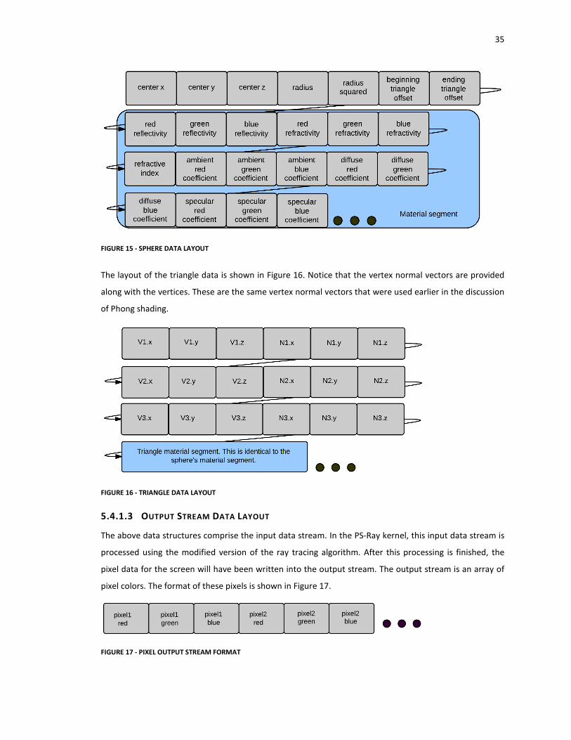
5.4.1.2 SPHERE AND TRIANGLE DATA LAYOUT

The next data structure of importance contains the bounding sphere data. This data structure contains all

the necessary information to do a sphere-intersection calculation. In addition, it contains two offset

values. The first offset value is the starting location of the embedded polygonal mesh’s triangles which

reside in the triangle buffer that is discussed below. The second value is the ending offset of the same set

of triangles. This enables the program to rapidly look up the appropriate set of triangles when an

intersection with a bounding sphere has occurred. Figure 15 details the sphere data structure layout. It is

a large contiguous float array.

35

FIGURE 15 - SPHERE DATA LAYOUT

The layout of the triangle data is shown in Figure 16. Notice that the vertex normal vectors are provided

along with the vertices. These are the same vertex normal vectors that were used earlier in the discussion

of Phong shading.

FIGURE 16 - TRIANGLE DATA LAYOUT

5.4.1.3 OUTPUT STREAM DATA LAYOUT

The above data structures comprise the input data stream. In the PS-Ray kernel, this input data stream is

processed using the modified version of the ray tracing algorithm. After this processing is finished, the

pixel data for the screen will have been written into the output stream. The output stream is an array of

pixel colors. The format of these pixels is shown in Figure 17.

FIGURE 17 - PIXEL OUTPUT STREAM FORMAT

36

This pixel output stream is transferred back to the host process and drawn to the screen using OpenGL’s

2-D drawing capabilities.

6 AMD RADEON MOBILITY 5870 GPU

The hardware specifications of the graphics card can dramatically affect the resulting timings. The

description of the hardware responsible for performing the calculations is provided below. The particular

GPU hardware used is the AMD Radeon Mobility 5870 [3]:

6.1 HARDWARE SPECIFICATIONS

• 1.04 billion 40nm transistors

• 800 Stream Processing Units

• GDDR5 memory interface

• PCI Express 2.1 x16 bus interface

• Engine clock speed: 700 MHz

• Processing power (single precision): 1.12 TeraFLOPS

• Data fetch rate (32-bit): 112 billion fetches/sec

• Memory clock speed: 1.0 GHz

• Memory data rate: 4.0 Gbps

• Memory bandwidth: 64 GB/sec

• Memory size: 1024 MB

• Thermal Design Power: 50 Watts

6.2 MEMORY CONSIDERATIONS

There are two aspects of the Radeon Mobility 5870’s memory architecture which limit the number of

threads that can be executing at a given moment. One is the number of registers in use. The other is the

amount of local data share per compute unit. On the Radeon Mobility 5870, here are the available

quantities of each:

• 256KB of registers per compute unit.

• 32KB of local data share per compute unit.

6.3 MAPPING THE RADEON MOBILITY 5870 TO THE OPENCL MEMORY MODEL

The implementation of the OpenCL Memory Model is dependent on the particular device on which the

OpenCL code will be executed. Figure 18 shows an approximate mapping of the Radeon Mobility 5870

hardware to the OpenCL memory model [29].

37

FIGURE 18 - MAPPING AMD RADEON HARDWARE TO THE OPENCL MEMORY MODEL

7 RESULTS

Results for this project were gathered for PS-Ray, PS-Triangle, and the single-threaded approach. In one

graph, a comparison is drawn across the timings of PS-Triangle, the single-threaded triangle intersection

code, and PS-Ray. The intent of this graph is to show the degree of speed-up achieved for the two

different parallelization attempts. The graph is shown in Figure 20. Notice that the PS-Ray kernel achieved

such an improvement that the chart x-axis had to be displayed using a logarithmic scale in order for the

PS-Ray kernel timings to be visible. The two other graphs of interest are the charts that detail the kernel

memory transfer times for both PS-Ray and PS-Triangle. We can see that the memory transfer times of PS-

Triangle are orders of magnitude larger than the memory transfer times for PS-Ray. These timings are

shown in Figure 21 and Figure 22.

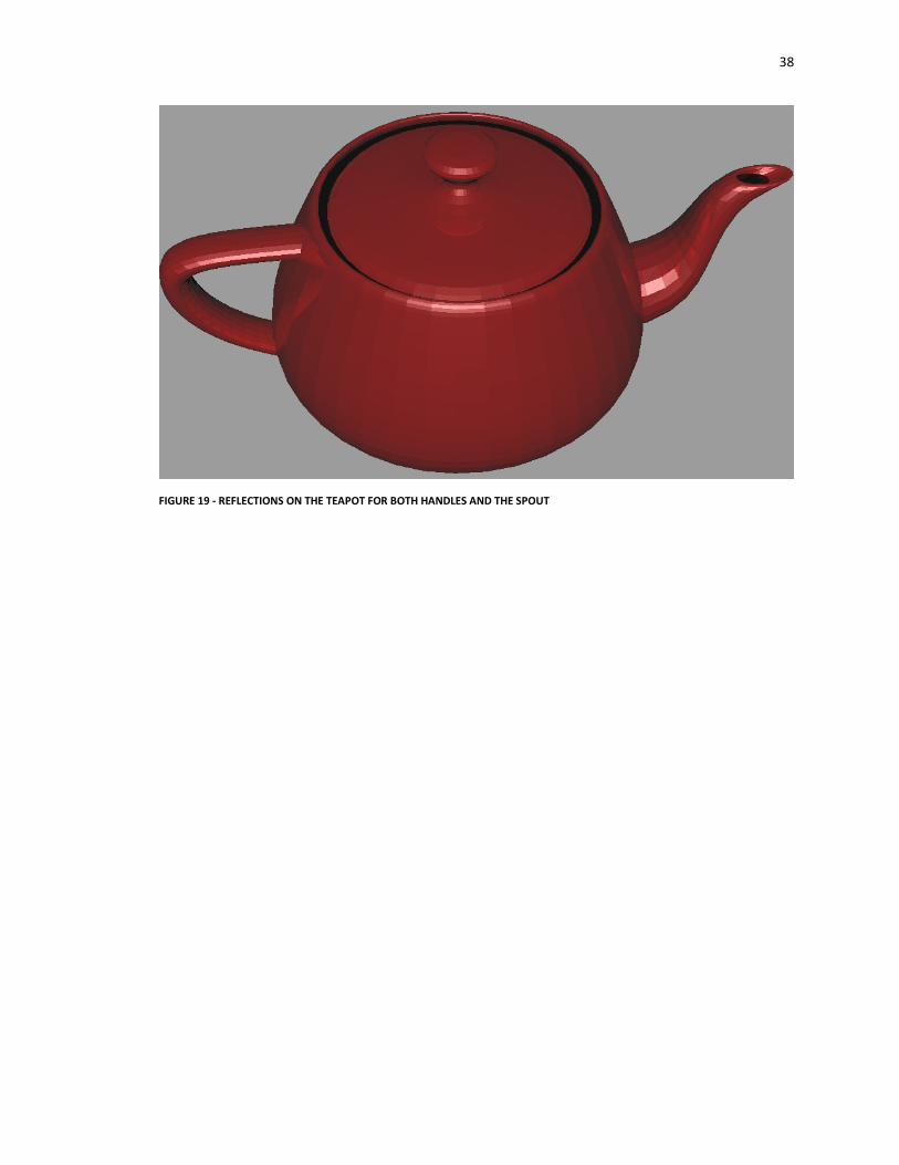
38

FIGURE 19 - REFLECTIONS ON THE TEAPOT FOR BOTH HANDLES AND THE SPOUT

39

FIGURE 20 - COMPARING TIMINGS OF PS-RAY AND PS-TRIANGLE TO SINGLE-THREADED TRIANGLE INTERSECTION

72,047

94,648

23,813

208,503

266,889

951,046

792,082

369

1,723

429

313,563

437,062

1,913,544

1,774,450

43

41

39

2,673

3,538

8,089

12,628

1E+00 1E+01 1E+02 1E+03 1E+04 1E+05 1E+06 1E+07

1 triangle - 14z(1)

3 triangles - 14z(3)

Cube - 14z(12)

Teapot - 14z(6320)

Al - 14z(7124)

F16 - 14z(9184)

Crocodile - 28z(34404)

Milliseconds Scaled Logarithmically

3-D

Ob

ject

(p

oly

go

n c

ou

nt)

All Ray Trace Timings

PS-Ray Single-threaded triangle Intersection PS-Triangle

40

FIGURE 21 - OPENCL MEMORY OPERATIONS FOR PS-RAY

FIGURE 22 - OPENCL MEMORY OPERATIONS FOR PS-TRIANGLE

7.1 SINGLE-THREADED TRIANGLE INTERSECTION

The single-threaded triangle intersection timings were obtained as a baseline comparison against both the

PS-Triangle kernel and the PS-Ray kernel.

0 5 10 15 20 25

time waiting for read

time writing rays

time writing view matrix

time writing matrix …

time writing sphere data

time writing triangle data

time writing scene data

time writing light data

Milliseconds

OpenCL Memory Operations - PS-Ray

Crocodile(34404)

F16(9184)

Al(7124)

Teapot(6320)

0 100000 200000

time waiting for read

time writing rays

time writing triangle data

Milliseconds

OpenCL Memory Operations -

PS-Triangle

Crocodile(34404)

F16(9184)

Al(7124)

Teapot(6320)

41

7.2 PARALLEL STRATEGIES VERSUS SINGLE-THREADED TRIANGLE INTERSECTION

The PS-Triangle kernel was able to decrease the time to intersect objects substantially. At the high end of

the polygon count, overall improvements in speed went from 1,774,450 milliseconds to 792,082

milliseconds, a speed-up of 224% for the crocodile when comparing the single-threaded triangle

intersection routine to PS-Triangle. However, the crocodile intersection code embedded in the PS-Ray

kernel took at most 12,628 milliseconds. This means that the speed-up for the intersection code

embedded in the PS-Ray kernel was at least 14051% faster than the single-threaded intersection code.

This clearly demonstrates the enormous processing throughput of GPUs. Note in Figure 20 that at the low

end of the polygon count, the setup and memory transfer overhead of PS-Triangle resulted in a situation

where the single-threaded intersection was actually faster than PS-Triangle.

8 FUTURE WORK

There are a number of ways in which the kernel execution speeds in this project may be optimized. These

include:

• Implementing more advanced data structures to optimize triangle intersection.

• Implementing the ray trace kernel iteratively to allow more ray reflections.

• Optimizing the kernels to use specialized functions and data types within the OpenCL language to

attempt to utilize more SIMD hardware – in other words, performing fine-grained kernel

optimization.

• Attempting to access the frame buffer within the OpenCL kernel so that the pixel data does not

have to be transferred back to the host for drawing.

• Storing all scene data in a texture to take advantage of caching. Reads from global memory are

minimally cached on the Radeon Mobility 5870.

9 CONCLUSIONS

It is very clear that parallelizing the ray tracing algorithm on GPU hardware leads to large speed-ups.

There are speed-ups for both PS-Triangle and PS-Ray. Unfortunately, even though speed-ups are possible

in both scenarios, the programmer is forced to choose one parallelization strategy or the other because to

the best of the author’s knowledge, nested kernel calls are not possible. An ideal solution would be to

parallelize using one thread per ray and then launch another kernel to handle the triangle intersection

segment of the ray thread [24]. The ability to invoke a stream-processing kernel from within another

stream-processing kernel may not be possible but it would address the issue of having to give up some

degree of parallelism to get more elsewhere. In other words, it is clear that although PS-Ray is much

42

faster, further speed-ups gained by PS-Triangle are not realized because one cannot execute a kernel

within a kernel, or nested kernel execution, using OpenCL [24].

There are, however, indications that OpenCL technology may be able accomplish nested kernel execution

soon. One of these indications is the fact that technologies like OpenMP and NVidia’s Kepler already

support launching threads within threads and kernels within kernels, respectively. It does not seem like a

large conceptual or technical leap to extend this idea to OpenCL kernels. The difficulty would appear to lie

in making this process seamless and cross-platform to the developer, given the current hardware

separation between CPUs and GPUs. That being said, it does appear that the underlying processor

technology is moving in a direction that may make this possibility a reality. This includes current attempts

by AMD to fuse the GPU and CPU cores on a single processor die as well as to unify the memory space

accessed by these two processor types [11]. Intel has also stated that it plans on adding more graphics

capability to its processor dies as well. With this tighter integration of memory and processor hardware,

making the distinction between launching threads within a thread and launching a kernel within a thread

may become unnecessary.

References

[1] T. Whitted, “An Improved Illumination Model for Shaded Display,” Communications of the ACM, vol.

23, no. 6, pp. 343–349, June 1980.

[2] P. L. Alvarez and S. Yamagiwa. Invitation to OpenCL. Presented at Networking and Computing (ICNC),

2011 Second International Conference on. 2011.

[3] ATI Mobility Radeon™ HD 5870 GPU Specifications. Retrieved from

http://www.amd.com/US/PRODUCTS/NOTEBOOK/GRAPHICS/ATI-MOBILITY-HD-5800/Pages/hd-5870-

specs.aspx

[4] A. Munshi, B. Gaster, T. G. Mattson, J. Fung, and D. Ginsburg, OpenCL Programming Guide, 1st

ed.

Addison-Wesley Professional, Jul. 2011.

[5] B. Gaster, L. Howes, D. Kaeli, P. Mistry, and D. Schaa, Heterogeneous Computing with OpenCL, 1st

ed.

Morgan Kaufmann, 2012.

[6] A. Bayoumi, M. Chu, Y. Hanafy, P. Harrell and G. Refai-Ahmed. Scientific and engineering computing

using ATI stream technology. Computing in Science & Engineering 11(6), pp. 92-97. 2009.

[7] M. Blazewicz, S. R. Brandt, M. Kierzynka, K. Kurowski, B. Ludwiczak, J. Tao and J. Weglarz. CaKernel - A

parallel application programming framework for heterogenous computing architectures. Scientific

Programming 19(4), pp. 185-197. 2011. Available:

http://ezproxy.library.ewu.edu:2048/login?url=http://search.ebscohost.com/login.aspx?direct=true&db=

a9h&AN=67655676&site=ehost-live&scope=site.

43

[8] R. P. Broussard, R. N. Rakvic and R. W. Ives. Accelerating iris template matching using commodity video

graphics adapters. Presented at Biometrics: Theory, Applications and Systems, 2008. BTAS 2008. 2nd IEEE

International Conference on. 2008.

[9] B. C. Budge, J. C. Anderson, C. Garth and K. I. Joy. A straightforward CUDA implementation for

interactive ray-tracing. Presented at Interactive Ray Tracing, 2008. RT 2008. IEEE Symposium on. 2008.

[10] Y. Torres, A. Gonzalez-Escribano and D. R. Llanos. Using fermi architecture knowledge to speed up

CUDA and OpenCL programs. Presented at Parallel and Distributed Processing with Applications (ISPA),

2012 IEEE 10th International Symposium on. 2012.

[11] M. Doerksen, S. Solomon and P. Thulasiraman. Designing APU oriented scientific computing

applications in OpenCL. Presented at High Performance Computing and Communications (HPCC), 2011

IEEE 13th International Conference on. 2011.

[12] P. Du, R. Weber, P. Luszczek, S. Tomov, G. Peterson and J. Dongarra. From CUDA to OpenCL: Towards

a performance-portable solution for multi-platform GPU programming. Parallel Computing 38(8), pp. 391-

407. 2012. Available:

http://ezproxy.library.ewu.edu:2048/login?url=http://search.ebscohost.com/login.aspx?direct=true&db=

a9h&AN=77286764&site=ehost-live&scope=site.

[13] A. Fawibe, O. Okobiah, O. Garitselov, K. Kavi, I. Nwachukwu, M. A. L. Dubasi and V. R. Prabhu.

Parabilis: Speeding up single-threaded applications by extracting fine-grained threads for multi-core

execution. Presented at Parallel and Distributed Computing (ISPDC), 2011 10th International Symposium

on. 2011.

[14] F. Jacob, D. Whittaker, S. Thapaliya, P. Bangalore, M. Mernik and J. Gray. CUDACL: A tool for CUDA

and OpenCL programmers. Presented at High Performance Computing (HiPC), 2010 International

Conference on. 2010.

[15] Jianbin Fang, A. L. Varbanescu and H. Sips. A comprehensive performance comparison of CUDA and

OpenCL. Presented at Parallel Processing (ICPP), 2011 International Conference on. 2011.

[16] R. Marroquim and A. Maximo. Introduction to GPU programming with GLSL. Presented at Computer

Graphics and Image Processing (SIBGRAPI TUTORIALS), 2009 Tutorials of the XXII Brazilian Symposium on.

2009.

[17] G. Martinez, M. Gardner and Wu-chun Feng. CU2CL: A CUDA-to-OpenCL translator for multi- and

many-core architectures. Presented at Parallel and Distributed Systems (ICPADS), 2011 IEEE 17th

International Conference on. 2011.

[18] C. Breshears. The Art of Concurrency: A Thread Monkey’s Guide to Writing Parallel Applications, 1st

edition. O’Reilly, May 2009.

[19] A. S. Nery, N. Nedjah, F. M. G. Franca and L. Jozwiak. A parallel ray tracing architecture suitable for

application-specific hardware and GPGPU implementations. Presented at Digital System Design (DSD),

2011 14th Euromicro Conference on. 2011.

[20] U. Ochsenfahrt and R. Salomon. CREMA: A parallel hardware raytracing machine. Presented at

Circuits and Systems, 2007. ISCAS 2007. IEEE International Symposium on. 2007.

44

[21] A. Segovia, Xiaoming Li and Guang Gao. Iterative layer-based raytracing on CUDA. Presented at

Performance Computing and Communications Conference (IPCCC), 2009 IEEE 28th International. 2009.

[22] Slo-Li Chu and Chih-Chieh Hsiao. OpenCL: Make ubiquitous supercomputing possible. Presented at

High Performance Computing and Communications (HPCC), 2010 12th IEEE International Conference on.

2010.

[23] J. E. Stone, D. Gohara and Guochun Shi. OpenCL: A parallel programming standard for heterogeneous

computing systems. Computing in Science & Engineering 12(3), pp. 66-73. 2010.

[24] Tong Li, P. Brett, R. Knauerhase, D. Koufaty, D. Reddy and S. Hahn. Operating system support for

overlapping-ISA heterogeneous multi-core architectures. Presented at High Performance Computer

Architecture (HPCA), 2010 IEEE 16th International Symposium on. 2010.

[25] R. O. Topaloglu and B. Gaster. GPU programming for EDA with OpenCL. Presented at Computer-Aided

Design (ICCAD), 2011 IEEE/ACM International Conference on. 2011.

[26] A.S. Glassner (1989). An Introduction to Ray Tracing. San Diego: Academic Press Inc.

[27] T. Leidi, T. Heeb, , M. Colla, and J. Thiran,, "Event-driven Scheduling for Parallel Stream Processing,"

Parallel Computing in Electrical Engineering (PARELEC), 2011 6th International Symposium on , vol., no.,

pp.36,41, 3-7 April 2011.

[28] T. Moller and B. Trumbore, “Fast Minimum Storage Ray Triangle Intersection” in J. Graphics Tools

(jgt) 2(1), 21-28 (1997).

[29] M. Daga, A. Aji, and W. Feng, “On the Efficacy of a Fused CPU+GPU Processor (or APU) for Parallel

Computing.” Symposium on Application Accelerators in High-Performance Computing, 2011. Available:

http://synergy.cs.vt.edu/pubs/papers/daga-saahpc11-apu-efficacy.pdf

[30] OpenCL Specification 1.2. Available at http://www.khronos.org

[31] K, Boydstun. Introduction to OpenCL [PDF document]. Web. 9 Aug. 2011. Available:

http://www.tapir.caltech.edu/~kboyds/OpenCL/opencl.pdf

[32] B. T. Phong, “Illumination for computer generated pictures,” Commun. ACM vol. 18, no. 6, pp. 311–

317, Jun. 1975. [Online]. Available: http://dx.doi.org/10.1145/360825.360839

45

VITA

Author: Coby B. Soss

Place of Birth: Spokane, Washington

Undergraduate Schools Attended: Spokane Community College,

Spokane Falls Community College,


Degrees Awarded: Bachelor of Science in Computer Science, 2002, Eastern Washington University,

Master of Science in Computer Science, 2013, Eastern Washington University

Honors and Awards: Graduate Assistantship, Computer Science Department, 2012-2013,


Star Award, TL-Pro, Itron Inc.

Star Award, Itron Enterprise Edition - Mass Market, Itron Inc.

Professional Experience: Software Engineer, Itron, Spokane, WA 2003-2012

Ray traced rendering using GPGPU devices

Documents

Transcript of Ray traced rendering using GPGPU devices