TBPoint: Reducing Simulation Time for Large-Scale GPGPU Kernels

Jen-Cheng Huang1, Lifeng Nai1, Hyesoon Kim2, and Hsien-Hsin S. Lee1

1School of Electrical and Computer Engineering2School of Computer Science

Georgia Institute of Technology

{jhuang34, lnai3, hyesoon.kim, leehs}@gatech.edu

Abstract— Architecture simulation for GPGPU kernels cantake a significant amount of time, especially for large-scaleGPGPU kernels. This paper presents TBPoint, an infrastruc-ture based on profiling-based sampling for GPGPU kernels toreduce the cycle-level simulation time. Compared to existingapproaches, TBPoint provides a flexible and architecture-independent way to take samples. For the evaluated 12 kernels,the geometric means of sampling errors of TBPoint, Ideal-Simpoint, and random sampling are 0.47%, 1.74%, and 7.95%,respectively, while the geometric means of the total sample sizeof TBPoint, Ideal-Simpoint, and random sampling are 2.6%,5.4%, and 10%, respectively. TBPoint narrows the speed gapbetween hardware and GPGPU simulators, enabling more andmore large-scale GPGPU kernels to be analyzed using detailedtiming simulations.

I. INTRODUCTION

Recently, one of the main scientific computing paradigms

in addition to Titan [1] and CSCS (Swiss National Super-

computing Center) [2] is General-purpose graphics process-

ing units(GPGPU), which has large-scale computing power.

To take advantage of this computing power, a wider range of

algorithms have been converted to GPGPU kernels. Future

workloads of GPGPU kernels will be much more complex

and much larger scale.

To design new architectures optimized for GPGPU ker-

nels, computer architects use a cycle-level simulator to gain

insights into kernel behaviors. Using cycle-level simulation

can help not only architects but also application developers

to understand the performance bottleneck in applications and

architectures.

However, because GPGPU architectures have many cores

to simulate, cycle-level simulation takes a significant amount

of execution time. Table I shows comparisons of GPGPU

execution times and expected simulation times of a cycle-

level GPGPU simulator. The GPGPU execution times are

from Burtscher et al. [3], and we used the Macsim simulator

for the GPGPU simulations [4]. The slowdown of Macsim

running on the Intel Ivy-bridge is around 80,000x compared

to native NVIDIA Quadro processors. Even for kernels

with a few seconds of running time, the simulation time

takes days. As a result of this slowdown, simulation is

an unattractive approach. Although most GPGPU kernels

Table ICOMPARISON OF GPGPU EXECUTION TIME AND SIMULATION TIME.

GPU TIME IS FOR NVIDIA QUADRO 6000.

Time NB SP SSSP PTA TSP DMR MM

GPU(msec)

28557 18779 7067 4485 4456 3391 881

Simulation 3.78weeks

2.48weeks

6.54days

4.15days

4.13days

3.14days

19.58hours

have short kernel sizes, the overhead comes from simulating

a massive number of threads. Because of the computing

power of GPU processors, an 80,000x slowdown is rea-

sonable. GPGPU applications can easily have 1GFLOPS

or even higher performance. If a simulator can simulate

1,000FLOPS/sec (which is similar to 10K instructions per

sec in typical cycle-level simulators), a 106 slowdown is

typical. To accelerate simulation time, one can parallelize a

cycle-level GPGPU simulator, but when large-scale GPGPU

systems are simulated, the required resources for such sim-

ulations become significant.

To reduce the time of CPU simulations, sampling tech-

niques have been widely used [5], [6], [7], but none have

been studied for GPGPU simulations. Although GPGPU

kernels seem to be similar to CPU multi-threaded applica-

tions, applying existing CPU sampling techniques, including

(1) systematic sampling and (2) profiling-based sampling

for multi-threaded applications, have some problems. For

example, systematic sampling [7], which takes samples

periodically, may lead to larger sampling sizes than required,

especially for kernels with regular execution patterns. In

addition, profiling-based sampling [5] requires a configura-

tion of a profiling platform similar to that of the simulated

platform, and sometimes the profiling may need to be

redone once the simulated configurations change, such as

the number of warps on an SM or the number of SMs,

incurring significant overhead.

A GPGPU application may have multiple kernels. For

each kernel, the simulation time can be reduced in two ways:

(1) reducing the number of kernel launches and (2) reducing

the simulation time of a kernel launch. Therefore, our goal is

to reduce the GPGPU simulation time on a per-kernel basis

2014 IEEE 28th International Parallel & Distributed Processing Symposium

1530-2075/14 $31.00 © 2014 IEEE

DOI 10.1109/IPDPS.2014.53

437

� �

���

���

���

���

���� ����

����

����

����

����

���

���

���

���

����

����

�������

����������

����

����

����

����

����

���

����

�������

����������

�������

������

������

������

���

���

���

���

���

�������

����������

���

���

���

���

����

����

����

����

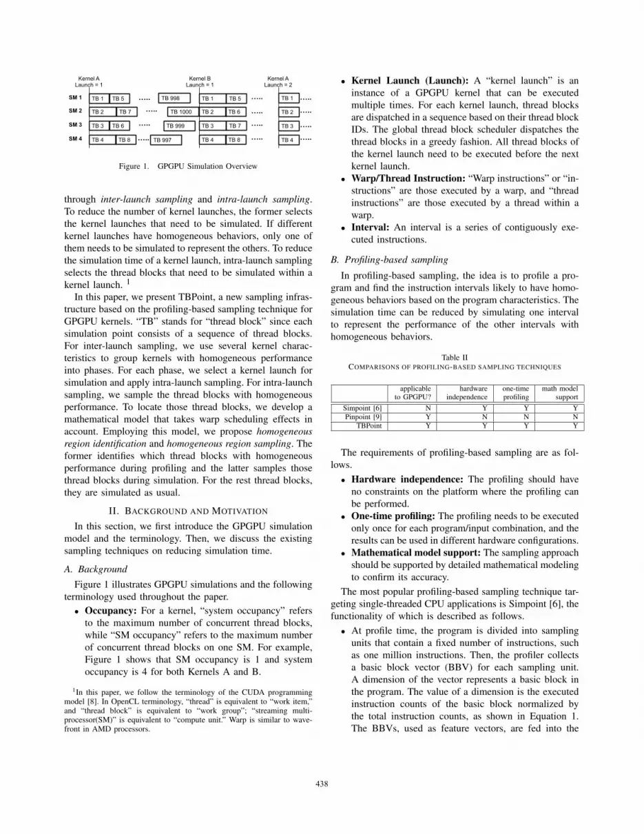
Figure 1. GPGPU Simulation Overview

through inter-launch sampling and intra-launch sampling.

To reduce the number of kernel launches, the former selects

the kernel launches that need to be simulated. If different

kernel launches have homogeneous behaviors, only one of

them needs to be simulated to represent the others. To reduce

the simulation time of a kernel launch, intra-launch sampling

selects the thread blocks that need to be simulated within a

kernel launch. 1

In this paper, we present TBPoint, a new sampling infras-

tructure based on the profiling-based sampling technique for

GPGPU kernels. “TB” stands for “thread block” since each

simulation point consists of a sequence of thread blocks.

For inter-launch sampling, we use several kernel charac-

teristics to group kernels with homogeneous performance

into phases. For each phase, we select a kernel launch for

simulation and apply intra-launch sampling. For intra-launch

sampling, we sample the thread blocks with homogeneous

performance. To locate those thread blocks, we develop a

mathematical model that takes warp scheduling effects in

account. Employing this model, we propose homogeneousregion identification and homogeneous region sampling. The

former identifies which thread blocks with homogeneous

performance during profiling and the latter samples those

thread blocks during simulation. For the rest thread blocks,

they are simulated as usual.

II. BACKGROUND AND MOTIVATION

In this section, we first introduce the GPGPU simulation

model and the terminology. Then, we discuss the existing

sampling techniques on reducing simulation time.

A. Background

Figure 1 illustrates GPGPU simulations and the following

terminology used throughout the paper.

• Occupancy: For a kernel, “system occupancy” refers

to the maximum number of concurrent thread blocks,

while “SM occupancy” refers to the maximum number

of concurrent thread blocks on one SM. For example,

Figure 1 shows that SM occupancy is 1 and system

occupancy is 4 for both Kernels A and B.

1In this paper, we follow the terminology of the CUDA programmingmodel [8]. In OpenCL terminology, “thread” is equivalent to “work item,”and “thread block” is equivalent to “work group”; “streaming multi-processor(SM)” is equivalent to “compute unit.” Warp is similar to wave-front in AMD processors.

• Kernel Launch (Launch): A “kernel launch” is an

instance of a GPGPU kernel that can be executed

multiple times. For each kernel launch, thread blocks

are dispatched in a sequence based on their thread block

IDs. The global thread block scheduler dispatches the

thread blocks in a greedy fashion. All thread blocks of

the kernel launch need to be executed before the next

kernel launch.

• Warp/Thread Instruction: “Warp instructions” or “in-

structions” are those executed by a warp, and “thread

instructions” are those executed by a thread within a

warp.

• Interval: An interval is a series of contiguously exe-

cuted instructions.

B. Profiling-based sampling

In profiling-based sampling, the idea is to profile a pro-

gram and find the instruction intervals likely to have homo-

geneous behaviors based on the program characteristics. The

simulation time can be reduced by simulating one interval

to represent the performance of the other intervals with

homogeneous behaviors.

Table IICOMPARISONS OF PROFILING-BASED SAMPLING TECHNIQUES

applicableto GPGPU?

hardwareindependence

one-timeprofiling

math modelsupport

Simpoint [6] N Y Y YPinpoint [9] Y N N N

TBPoint Y Y Y Y

The requirements of profiling-based sampling are as fol-

lows.

• Hardware independence: The profiling should have

no constraints on the platform where the profiling can

be performed.

• One-time profiling: The profiling needs to be executed

only once for each program/input combination, and the

results can be used in different hardware configurations.

• Mathematical model support: The sampling approach

should be supported by detailed mathematical modeling

to confirm its accuracy.

The most popular profiling-based sampling technique tar-

geting single-threaded CPU applications is Simpoint [6], the

functionality of which is described as follows.

• At profile time, the program is divided into sampling

units that contain a fixed number of instructions, such

as one million instructions. Then, the profiler collects

a basic block vector (BBV) for each sampling unit.

A dimension of the vector represents a basic block in

the program. The value of a dimension is the executed

instruction counts of the basic block normalized by

the total instruction counts, as shown in Equation 1.

The BBVs, used as feature vectors, are fed into the

438

clustering algorithm, k-means, to group the sampling

units into clusters. For each cluster, a sampling unit

that is selected as the simulation point represents the

performance of the other units in the cluster.

• At simulation time, only the sampling units selected

as simulation points need to be simulated. The other

sampling units can be skipped by fast-forwarding. Each

simulation point could have different weights, depend-

ing on the number of sampling units in the cluster. The

overall CPI can be predicted by Equation 1.

BBV =< BB1 :#BB1 insts

#insts, BB2 :

#BB2 insts

#insts...BBN :

#BBN insts

#insts>

Total CPI =∑

i∈phases

(representative unit CPIi × phase weighti)

phase weighti =#sampling unitsi

total sampling units(1)

Since GPGPU kernels can be considered as multithreaded

applications, Pinpoint [9], an extension of Simpoint for

sampling multi-threaded applications, could be applicable

to GPGPU kernels. In Pinpoint, BBVs are collected on

a per-thread basis by actually executing all threads on a

real system. However, it does not meet the requirements of

profiling-based sampling for the following reasons.

• The profiling needs to be redone for different hardware

configurations since the profiling results (simulation

points) can only be applied to the simulated platform,

which has the same hardware configurations as the

profiling platform.

• Although the BBV has a strong correlation with perfor-

mance in single-thread applications [10], it is uncertain

whether the same would be true for GPGPU kernels

because of the warp scheduling effect.

Table II summarizes the comparisons of different

profiling-based sampling techniques. To satisfy all of the

requirements of profiling-based sampling, we propose a

sampling approach, TBPoint. In terms of hardware inde-

pendence, TBPoint uses GPUOcelot [11] as the profiling

tool, which performs the functional simulations of GPGPU

kernels and collects the information about each thread block.

In terms of one-time profiling, for different hardware con-

figurations, such as a different number of warps and SMs,

TBPoint simply needs to re-perform clustering while reusing

the profiling results, incurring low overhead. To model the

warp scheduling effect, we use a Markov Chain model that

accounts for the performance impact of the effect.

III. INTER-LAUNCH SAMPLING

Using hierarchical clustering [12], inter-launch sampling

groups the kernel launches with homogeneous performance.

We simulate only one kernel launch within each cluster and

predict that the performance of the other kernel launches

within each cluster will be the same as the simulated launch,

thus reducing simulating time.

� �

������

�����

�

�����������

���������

������

�����

�

������

�����

�

������

�����

�

������

������

�

������

������

�

�������

����

��

�������

����

�

�������

����

���

�������

����

��

�������

����

���

����

����

������� �

������� �

���

���

���

�������������������

��� ������������

!�!���"����

Figure 2. Procedure of Inter-Launch Sampling.

Figure 2 shows the procedure of inter-launch sampling.

First, each kernel launch is represented as a feature vector,

which is the input to the clustering algorithm. A feature

vector describes the characteristics of a kernel launch that

contains four features (described below), each of which

belongs to one dimension of the vector. Then, hierarchical

clustering processes the feature vectors and groups them into

clusters. Since each feature vector represents a kernel launch,

the kernel launches within the same cluster are believed to

have homogeneous performance (IPCs).

The design of feature vectors is important since a feature

vector should correctly describe the characteristics of a

kernel launch so that the hierarchical clustering can group

the kernel launches with homogeneous performance into a

cluster. The features with which we chose to compose a

feature vector and their performance impact are shown as

follows.

• Kernel launch size: The number of thread instructionsof a kernel launch is used as a feature to capture the

size of a kernel launch.

• Control flow divergence: Because simply capturing

the number of thread instructions of a kernel launch

does not reflect its degree of control flow divergence,

the number of warp instructions of a kernel launch

is used as a feature to capture the degree of control

flow divergence. Even if two kernel launches have the

same number of thread instructions, they may have

different IPCs due to different degrees of control flow

divergence. For example, Kernel Launch 1 executes

32 thread instructions in one warp instruction, while

Kernel Launch 2 executes 32 thread instructions in 32

warp instructions.

• Memory divergence: Because kernel launches with

different numbers of memory requests are likely to

have different IPCs, the number of memory requestsof a kernel launch is used as a feature to capture the

degree of memory divergence. The degree of memory

divergence is independent of the number of thread

blocks and the control flow divergence. For example,

a warp instruction that contains 32 thread instructions

can issue at least one and up to 32 memory requests if

none of the accesses can be coalesced.

• Thread block variations: The coefficient of variations

439

(CoV) of thread block sizes of a kernel launch is used as

a feature to capture the variations of thread block sizes.

Thread block size is defined as the number of thread

instructions in a thread block. All the above features are

designed as if only one thread block were running per

kernel launch. However, a kernel launch typically has

multiple thread blocks, and different thread blocks may

have a different number of instructions. For example,

let’s assume that kernel launch 1 has two thread blocks

with the number of thread instructions 100 and 100,

respectively, and that kernel launch 2 has two thread

blocks with the number of thread instructions 160 and

40, respectively. Even though both kernel launches may

have the same size (200 thread instructions), they may

perform differently because of distinct thread block

interleaving situations.

Equation 2 shows the inter-feature vector composed of the

above features, each of which is normalized with its average

value across all kernel launches so that they have the same

order of magnitude.

For kernel launch i,

inter feature vectori =< Kernel Launch Size, Control Flow Divergence,

Memory Divergence, Thread Block Variations >

=<#thread instsi

avg thread insts,

#warp instsi

avg warp insts,

#mem reqsi

avg mem reqs, CV TB size >

(2)

Hierarchical clustering takes all inter-feature vectors and

groups them into clusters. For each cluster, the kernel launch

with the inter-feature vector closest to the center of the

cluster is selected as a simulation point that will be sampled

by intra-launch sampling.

We chose hierarchical clustering instead of the k-means

algorithm used by Simpoint for the following reason. The

number of clusters can be determined automatically by

setting the distance threshold σ, which is the maximum

distance between any two points in a cluster. The higher

threshold results in fewer clusters, which decreases the total

sample size, but the variations within each cluster could be

higher, which increases the sampling errors. The appropriate

value of the distance threshold depends on the required

accuracy and hardware configurations. On the other hand,

the k-means algorithm requires a pre-defined number of

clusters as an input, which needs another index, such as

Bayesian information criterion (BIC) score, to set.

The proposed inter-feature vector has the following ad-

vantages over BBVs, which were used in Simpoint. First, it

provides more insight into performance behavior. We found

that BBVs are less correlated with performance on GPGPU

programs. GPGPU kernels often have very few basic blocks

and even the same basic blocks show very distinct per-

formance behaviors because of memory divergence, thread

block variations, and other behaviors. Furthermore, the same

kernel can be launched multiple times but each invocation of

� �

���� ����

����

����

����

����

����

����

���

���

����

����

�����

������

�������

������

������

������

�������

�����

������

�

�����

�����

�����

�� ��������

������

�� ����� ���

�� ����� �� �����

Figure 3. Intra-Launch Sampling

the kernel shows particular behaviors, e.g., reduction kernel.

Hence, although BBVs can be useful to detect program

behavior, the sources of performance variations cannot be

solely obtained through BBVs. On the other hand, the

proposed vector is also more computationally efficient since

it has only four dimensions, while the BBV has a number

of dimensions equal to the number of basic blocks in the

kernel launch. 2

IV. INTRA-LAUNCH SAMPLING

Once inter-launch sampling selects a kernel launch from

each cluster for simulation, intra-launch sampling can further

reduce the simulation time by sampling the selected kernel

launch.

Figure 3 shows a high-level view of intra-launch sampling.

Within a kernel launch, our goal is to sample homogeneousregions, which have homogeneous performance across mul-

tiple thread blocks. In a homogeneous region, a few thread

blocks are simulated while the others are skipped so as

to reduce the simulation time. The IPC collected from the

simulated thread blocks is predicted to be the IPC of the

entire homogeneous region. The thread blocks not in any

homogeneous regions are simulated as usual.

The design presents the following challenges.

• How do we define a homogeneous region? (Section

IV-A)

• During profiling, how do we identify the location of a

homogeneous region? (Section IV-B1)

• During simulation, how do we sample a homogeneous

region? (Section IV-B2)

A. The Design of Intra-Launch Sampling

Our design of intra-launch sampling identifies a homo-

geneous region through the mathematical model that quan-

tifies the IPC variations under different warp interleaving

situations that we assume are caused by variable memory

latencies due to resource contention and/or queuing delay.

Based on our model, such IPC variation has proven to be

2The BBV can be added as another feature for improving accuracy withthe cost of increased total sample size. The study of such extension is leftfor our future work.

440

� �

��������

��

�����

�

�

����

��

����

��

Figure 4. The State Diagram of a Warp. p = mem inststotal insts

,Mk ∼ N(μ, σ2)

small. The IPC of a homogeneous region can be predicted

as equal to one of its homogeneous intervals. The definitions

and proofs are as follows.Definition 4.0:• p is the stall probability that is the probability of a

warp being stalled, and M is the average stall cyclesconsumed by a stall event. p is modeled as a constant

while M is modeled as a random variable following

Gaussian distribution. N is the number of warps in an

SM.

• A homogeneous interval is a sequence of executed

instructions from concurrent warps, and each warp has

the same p and M.

• A homogeneous region is the region with consecutive

homogeneous intervals with the same p and M.

Lemma 4.1: The IPC variation of a homogeneous interval

under different warp interleaving situations caused by ran-

dom variable M is within a 10% difference of the average

IPC.Definition 4.0 shows all definitions that are required for

the model. As an example of the input parameter p and M,

let us assume that a warp has 10% long latency instructions,

and each of which consumes 400 cycles on average. Then, p

is a constant equal to 0.1. M is a random variable following

N(μ, σ) where the σ = 0.1×μ1.96 so that 95% of randomly

picked Ms is within ±10% of μ (400 cycles). Figure 4 shows

the state diagram of a warp, which is the basic building block

of the model.Lemma 4.1 is proven by modeling the IPC variation of

a homogeneous interval that includes two steps. First, the

IPC of a homogeneous interval is predicted by the Markov

chain, which considers the warp interleaving effect. Second,

the IPC variation caused by variable M can be predicted by

the Monte Carlo method, which performs the Markov chain

analysis a finite number of times.

Si,j =

N∏x=1

f(Ai[x], Aj[x]), Ai[x], Aj[y] ∈ {0, 1}, 0 ≤ i, j < 2N − 1

f(Ai[x], Aj[x]) =

{Ai[x]× p + (1− Ai[x])× 1

Mx, Ai[x] �= Aj[x]

Ai[x]× (1− p) + (1− Ai[x])× (1− 1Mx

), Ai[x] = Aj[x]

Vi =< R0, R1, R2...R2N−1 >=< 0, 0, 0, ...1 >

Vs = limn→∞ ViT

n

T =

⎡⎢⎢⎣

S0,0 S0,1 ... S0,2N−1

S1,0 S1,1 ... S1,2N−1

... ... ... ...S2N−1,0 S2N−1,1 ... S2N−1,2N−1

⎤⎥⎥⎦

IPC = 1.0× (1− R0)(3)

To predict the IPC under different warp interleaving

situations, the Markov chain is used, as shown in Equa-

tion 3. Let us assume that each warp is an independent and

identically distributed (i.i.d.) random variable. The size of

the transition matrix is 2N×2N, as each warp has two states

and the number of warps in an SM is N. The transition

probability Si,j is the element of the transition matrix T and

its calculation is shown as follows. For example, S6,2 is the

transition probability from 0110 (6) to 0010 (2), in which

each bit represents a warp such that Warp 1 is the most

significant bit, Warp 2 is the second most significant bit, and

so on. In this case, S6,2 is the probability of Warp 2 transiting

from a runnable to stall state while other warps remain in

their current states since the second most significant bit is

flipped from 1 (runnable) to 0 (stall) while other bits remain

unchanged. After constructing the transition matrix, steady

state vector Vs and the expected IPC can be calculated using

Equation 3. The initial state vector Vi is < 000...1 > since

all warps are initially in the runnable states.

After the IPC is predicted by Markov chain model, we

need to quantify the IPC variation caused by variable M

using the Monte Carlo method, which performs the Markov

Chain a finite number of times (samples). For each sample,

M of each warp is randomly selected. The total number

of samples is set to 10,000. Figure 5 shows that the IPC

variation of a homogeneous interval is low since more than

95% of the samples have less than a 10% difference of the

average IPC.

By Lemma 4.1 , we can conclude that for a homogeneous

interval or region, its IPC is stable and not sensitive to

different warp interleaving situations. The model provides a

theoretical range of IPC values of different warp interleaving

situations caused by random variable Ms of a homogeneous

interval: For more than 95% of samples with randomly

picked Ms, the IPCs are within 10% error of the average

IPC.

Our model shares some similarities with other Markov

chain models that predicts the IPC of a multithreaded

core [13]. However, in these models, M is modeled as a

constant, which is unrealistic for the stall events such as

DRAM accesses, which have variable latencies resulting

from a queuing delay. Our model provides a detailed study

that examines IPC variation caused by variable stall latencies

M.

B. Implementation of Intra-Launch Sampling

Our implementation of intra-launch sampling has two

components: (1) homogeneous region identification and (2)

homogeneous region sampling. The former identifies the

homogeneous regions during profiling. The locations of

homogeneous regions are stored in the homogeneous region

table. The latter samples the homogeneous regions using the

homogeneous region table during simulation.

441

� �

�� �� ��� ��� ��� �����

���

���

���

���

����

��������� ��������� ��������� ���������

��������� ��������� ��������� ���������

��������� ��������� ��������� ���������

��� ����������������� ���������

Figure 5. IPC Variation (Each legend shows the p, M, and N values. Forexample, p0.05M100N4 means p = 0.05, M = 100 and N = 4)

� �

����

����

����

����

����

����

�����

�����

�����

�����

�����

����

����

�����

�����

�����

�����

�����

�����

�����

����

���

���

����

�����

����

����

�����

�����

�����

�����

�����

� ���

�� �

� ���

�� �

� ���

�� ���

� ���

�� ���

� ���

�� �

� ���

�� �

� ���

�� �

� ���

�� �

� � � � ���

� � � � � �

�����������������������

����#���#��������#�

$�#��

����#��

�#��������#�

$�#���

����������

�#%#����#���

����#�

�#��������#�

� � ���������&'

����#��&'

��#��

�������

�����

����

Figure 6. Example of Homogeneous Region Identification

Since profiling is done at the thread block level, to reduce

the complexity of implementation, we change the definitions

of homogeneous regions and intervals from the warp level

to the thread block level. For example, the definition of

a homogeneous interval becomes a sequence of executed

instructions from concurrent thread blocks with the same p

and M.

1) Homogeneous Region Identification: The basic idea

of homogeneous region identification is shown as follows.

During profiling, because the thread blocks within a homo-

geneous region must have the same p and M, identifying

a homogeneous region requires the information of which

thread blocks are concurrently running at any time period.

Since we observe that thread blocks having closer thread

block IDs are likely to be running concurrently, we group

several thread blocks with closer IDs into an ”epoch”, as

shown in Equation 4. The size of an epoch is equal to the

system occupancy. For example, the epoch size of Figure 3

is four thread blocks. An epoch with all thread blocks

that have equal p and M is a homogeneous interval. If

consecutive epochs has equal p and M, a homogeneous

region is constructed by those epochs.

epochi = {TBoccupancy∗i, TBoccupancy∗i+1...

TBoccupancy∗i+occupancy−1}(4)

Implementing the idea contains three steps: (1) epoch vec-

tor construction, (2) epoch clustering, and (3) homogeneous

region construction.

Epoch vector construction: Epoch vector construction

converts each epoch into an intra-feature vector that is used

to find epochs with the same average stall probability (p)

and average stall cycles (M). An intra-feature vector uses the

stall probability of an epoch, which is the stall probability

averaged over all thread blocks in an epoch, as the only

feature. The stall probability (p) and average stall cycles (M)

of each thread block are collected as follows. Equation 5

illustrates intra-feature vector.

• Stall probability (p) The stall probability of a thread

block is approximated using the ratio of the number

of memory requests to the total number of instructions

collected for each thread block. The types of memory

requests that we consider are global and local memory

accesses.

• Average stall cycles (M) The average stall cycles of

a thread block is not collected since the average stall

cycles M cannot be determined without detailed timing

simulations. Instead, we assume that if two epochs have

the same stall probability (p) for the thread blocks, the

average stall cycles (M) from two epochs are also equal

since the same kernel code is executed.

Xepochj= {xTBi

|TBi ∈ epochj}xTBi

= The number of memory requests in TBi

Yepochj= {yTBi

|TBi ∈ epochj}yTBi

= The number of warp instructions in TBi

stall probabilityepochj=

∑TBi∈epochj

(xTBiyTBi

)

|Xepochj|

intra feature vectorepochj=< avg stall probabilityepochj

>

variance factorepochj= max(CoV(Xepochj

), CoV(Yepochj))

(5)

Epoch clustering: Hierarchical clustering groups epochs

using their intra-feature vectors and generates a cluster

ID for each epoch. The epochs with the same cluster ID

are believed to have the same p and M. However, some

thread blocks with distinct stall probabilities and/or number

of instructions, called outlier thread blocks, in an epoch

may result in different performance and they may not be

captured by hierarchical clustering. Thus, after grouping,

post-processing must be done to capture the epochs with

outlier thread blocks using the variation factor (VF), which

quantifies the dissimilarity between thread blocks using the

coefficient of variation (CoV), as shown in Equation 5.

If the variation factor of an epoch is larger than some

threshold, indicating the existence of outlier thread blocks,

the epoch should be removed from the cluster it belongs to

and assigned its own cluster.

Homogeneous region construction: After every epoch

has been assigned a cluster, a homogeneous region is con-

structed for a sequence of consecutive epochs that share

the same cluster. The ID of the cluster, used as the region

ID, is assigned to every thread block in a region. For

every homogeneous region, all its thread blocks and their

corresponding region IDs are stored in the homogeneous

region table, as shown in Table III.

442

� �

�����

�����

�����

�����

�����

�����

�����

�����

�����

�����

�����

������� ��������

�����

�����

!"���������� ����

�����

�����

�����

�����

�����

�����

���

���

���

���

���������������

�����

�����

�����

�����

�� � � �� � � �� � � �� � �

��������� ���������

������ ����

������ �!

������� ��������"#��

����������������������$

�%��

�%�&

�%�!

�%�'

�����(����

���������

�������� ��������

Figure 7. Example of Homogeneous Region Sampling. SU = samplingunit ID. RID = homogeneous region ID.

Figure 6 illustrates homogeneous region identification.

During epoch vector construction, because the first four

epochs have the same stall probability (0.2), their intra-

feature vectors are equal. Similarly, the remaining four epoch

have the same intra-feature vectors. During epoch clustering,

the first four epochs are grouped into one cluster while the

remaining epochs are grouped into the other cluster. Because

the variation factors of the third and fourth epochs are high

indicating the existence of outlier thread blocks, the epochs

are removed from the cluster. During homogeneous region

construction, two homogeneous regions are identified. The

first and second epochs belong to one homogeneous region

while the last four epochs belong to the other homogeneous

region.

Table IIIEXAMPLE OF HOMOGENEOUS REGION TABLE

Region ID Start TB ID End TB ID

1 0 402 50 120

2) Homogeneous Region Sampling: After the locations

of homogeneous regions are determined, we need to sample

homogeneous regions using the homogeneous region table

during simulation. The basic idea is to simulate only a few

thread blocks within a homogeneous region and skip the

other thread blocks in the region. The IPC of the region is

predicted as equal to the IPC of the simulated thread blocks.

For the thread blocks not in any homogeneous regions, they

are simulated as usual.

To sample a homogeneous region, we must define the size

of a sampling unit. The IPC of a sampling unit represents

the IPC of a homogeneous region. We define a sampling

unit as the interval between the start and end of a specified

thread block. The first specified thread block is the very

first dispatched thread block when the simulation begins.

Once the current one is retired, another thread block will

be specified. Compared to the design of sampling units

with a fixed number of instructions, this design ensures

that every sampling unit has a similar stall probability

since the specified thread block executes the whole kernel

code, which potentially captures the behaviors of the whole

kernel. In addition, as it requires no instruction counting for

determining the length of an interval, the design simplifies

the complexity of implementation.

Sampling a homogeneous region contains three steps: (1)

entering, (2) sampling and (3) exiting a homogeneous region.

Each step is described as follows.

Entering: Entering a homogeneous region happens when

all concurrently running thread blocks belong to the same

homogeneous region in the homogeneous region table.

Sampling: Once a homogeneous region is entered, sam-

pling a homogeneous region breaks into two periods: (1)

a warming period and (2) a fast-forwarding period. During

the warming period, the thread blocks are simulated as usual,

and the IPC of the current sampling unit is recorded. If the

IPC difference between the current and previous sampling

units is less than 10%, the cache states are considered

stable and the fast-forwarding period begins. Otherwise, the

warming period continues. During fast-forwarding period,

the dispatched thread blocks are skipped while the IPC of

the homogeneous region is predicted to be the IPC of the

last sampling unit in the warming period.

Exiting: The homogeneous region exits when the newly

dispatched thread block region ID differs from the current

homogeneous region ID. Then, the simulation continues.

Figure 7 illustrates homogeneous region sampling. Ini-

tially, because not all thread blocks of sampling unit 1 are

in a homogeneous region, the homogeneous region is not

entered until sampling unit 2. Sampling units 2 and 3 belong

to the warming period of sampling step. Since the IPC

difference between sampling units 2 and 3 is less than 10%,

the cache states are stable and the fast-forwarding period

starts at sampling unit 4. During fast-forwarding period, the

remaining thread blocks from the region are skipped. The

homogeneous region exits when the thread block that does

not belong to the region is dispatched. Then the simulation

continues as usual.

Table IV summarizes how the overall IPC is predicted

when inter-launch and intra-launch sampling techniques are

applied. Note that these two sampling techniques, which are

orthogonal, can be applied independently.

V. EVALUATION

A. Evaluation Configurations

We use Macsim, a cycle-accurate trace-driven simulator,

as our simulation platform in which the homogeneous region

sampling technique is implemented. The detailed simulation

configurations, based on the NVIDIA Fermi architecture, are

listed in Table V.

Table VI shows the evaluated benchmarks, long running

benchmarks from several benchmark suites. For those with

multiple kernels, we select the kernel that has the longest

running time. Figure 8 depicts our method of classifying

regular and irregular kernels based on thread block sizes.

443

Table IVIPCS OF INTER-LAUNCH AND INTRA-LAUNCH SAMPLING

Inter-Launch sampling

total CPI =∑

clusterk∈clusters

representative kernel launch CPIclusterk×

cluster weightclusterk

cluster weightclusterk=

∑launchp∈clusterk

#kernel launch instslaunchp

total insts

Intra-Launch sampling

launch insts =∑

i∈simulated TBs

#TB instsi +∑

j∈skipped TBs

#TB instsj

launch cycles =∑

i∈simulated TBs

#TB cyclesi +∑

j∈skipped TBs

#TB instsj

homogeneous region IPCj

launch CPI =launch cycles

launch insts

� ����

��������������������������������������������������

����

���

������������������������������������������������������������������

����

���

������������

������������

���

��

���

��

���

��

��

���

���

���

���

Figure 8. Different Kernel Types. (a) Regular. (b) Irregular kernel. A reddot indicates the start of a kernel launch while a blue dot indicates a threadblock. Thread block size ratio is the thread block size, which is the numberof thread instructions in a thread block, normalized by the average threadblock size across all thread blocks.

The X axis is the thread block ID, while the Y axis is the

thread block size. Types (a) is a regular kernel since the

thread block sizes exhibit particular patterns. Type (b) is an

irregular kernel.

Table VSIMULATION CONFIGURATION.

Number of cores 14

Front EndFetch width: 1 warp-instruction/cycle,4KB I-cache, 5 cycle decode

Execution core

1.15 GHz,1 warp-instruction/cycle,32-wide SIMD execution unit,in-order schedulinginstruction latencies are modeledaccording to the CUDA manual

On-chip caches16 KB software managed cache16 KB L1 cache, 128B line, 8-way assoc768 KB L2 cache, 128B line, 8-way assoc

DRAM1.15GHz, 2 KB page,16 banks, 6 channels,FR-FCFS scheduling policy

We evaluate the following sampling techniques.

• TBPoint: This approach applies both inter-launch sam-

pling and intra-launch sampling. The distance threshold

� �

�

�

�

�

�

��

��

��

��� ������� ���� ������ ����

���

����� �������

Figure 9. Overall IPC. (The overall IPC is defined as∑

k∈SMs#warp instsk

#cyclesk).

� �

��

���

���

���

���

����

��� ������� ���� ������

���������������� � ��� � ���

Figure 10. Total Sample Size (Ratio). (The total sample size is defined

as∑

k∈SMs#simulated warp instsk

#warp instsk).

of hierarchical clustering is for the former 0.1 and for

the latter 0.2. The variation factor is 0.3.

• Random sampling (Random): We conduct a full

simulation in which we collect IPC for every sampling

unit with one million instructions and randomly select

10% sampling units.

• Ideal-Simpoint: For Ideal-Simpoint, we collect the

BBV and IPC for every sampling unit with one million

instructions. Then, we use the Simpoint tool for cluster-

ing BBVs and simulation point selection. The overall

IPC can be calculated using Equation 1. The difference

between Ideal-Simpoint and the original Simpoint is

that the full timing simulation is performed in Ideal-

Simpoint to collect BBV from concurrent warps in

every sampling unit, so Ideal-Simpoint is not a viable

solution for the GPGPU platform. Without a full timing

simulation, what instructions are executed by each warp

in every sampling unit is unknown because of the

unpredictable effect of warp scheduling.

• Full: The total IPC is collected through the full simu-

lation with no sampling techniques applied.

B. Comparisons

Figure 9 shows the total IPCs of three approaches. The

geometric mean of the sampling errors of Random, Ideal-

Simpoint, and TBPoint are 7.95%, 1.74%, and 0.47%, re-

spectively. Random has a much higher error rate, especially

for the irregular kernels. The sampling errors of Ideal-

444

Table VIEVALUATED BENCHMARKS (TYPE I: IRREGULAR KERNEL, TYPE II: REGULAR KERNEL)

BFS SSSP MST MRI-Gridding SPMV LBM CFD Kmeans Hotspot StreamCluster BlackScholes convolutionSeparable

Suite lonestar lonestar lonestar parboil parboil parboil rodinia rodinia rodinia rodinia sdk sdk

Type I I I I II II II II II I II II

Number of Kernel launches 41 49 9 7 50 6 100 30 1 21 87 11

Number of Thread blocks 10619 12691 2331 18158 38250 108000 50600 58080 1849 2688 41760 202752

Abbreviation bfs sssp mst mri spmv lbm cfd kmeans hotspot stream black conv

Simpoint and TBPoint are less than 2% for all benchmarks,

except mst. Ideal-Simpoint has the highest errors (8.5%)

for mst because the BBVs cannot detect the thread-level

parallelism (TLP) changes caused by the outlier thread

blocks, which have considerably more instructions than the

others.

Figure 10 shows the total sample size of the three ap-

proaches. The geometric mean of the total sample size of

Random, Ideal-Simpoint, and TBPoint are 10%, 5.4%, and

2.6%, respectively. For regular kernels, while Random takes

many more samples than needed since it cannot detect the

regularity in a kernel, the other approaches have a similar

sample size. For irregular kernels, the average sample size

of TBPoint is 50.5% of the sample size of Ideal-Simpoint

because the intra-feature vector captures changes in stall

probabilities. mst has a high sample size (55%) because to

achieve high accuracy, TBPoint needs to simulate the epochs

with outlier thread blocks.

� �

�������

������ �����

�������

������ �����

�������

������ �����

�������

������ �����

�������

������ �����

�������

������ �����

�������

������ �����

�������

������ �����

�������

������ �����

�������

������ �����

�������

������ �����

�������

������ �����

�

����

�� �

���

� ���

���

�������

���

����

��

��

����

��

���

����

������������� ���� ������������ ����

���������

������� �����

Figure 11. Breakdown of the Relative Percentage of Skipped Instructionsfrom Inter-Launch and Intra-Launch Sampling.

Figure 11 shows the relative percentage of skipped in-

structions from inter-launch and intra-launch sampling. For

regular kernels, most savings come from the inter-launch

sampling for both approaches because all kernel launches

are homogeneous, except binomial and hotspot, which only

have one kernel launch. For irregular kernels, the percentage

of inter-launch sampling decreases since different kernel

launches are not homogeneous. For mst, most savings come

from intra-launch sampling since different kernel launches

have different sizes. For stream, hundreds of homogeneous

kernel launches cause the most savings to come from inter-

launch sampling.

� �

��

��

��

��

��

���

���

���

���

���� ���� ����� ����� ����� �����

������

������������

Figure 12. Sampling Errors of Different Hardware Configurations. W isthe number of warps in an SM, and S is the number of SMs

� �

�

�

��

��

��

���� ���� ����� ����� ����� ��������� ��������

������� ���������

Figure 13. Total Sample Sizes (Ratios) of Different Hardware Configura-tions

C. Sensitivity Analysis

TBPoint can quickly adapt to the hardware configurations

with system occupancy change, such as those with a different

number of SMs or warps. The required computations are

shown as follows. For intra-launch sampling, the homoge-

neous region identification needs to be redone since the

epoch size changes according to system occupancy. The

overhead is small compared to that of profiling all thread

blocks using GPUOcelot, which only needs to be done

once, regardless of the system occupancy. For inter-launch

sampling, because the kernel characteristics do not change

when the system occupancy changes, the clustering of inter-

launch sampling needs to be done only once.

Figure 12 shows the errors of the hardware configurations

with different system occupancies. The maximum error rate

is less than 14%. Some kernels exhibit high variation in the

error rate for the following reasons. First, the cache states are

not fully constructed because of the lack of cache accesses

during fast-forwarding, leading to inaccurate IPC after fast-

forwarding. Second, if a kernel is more memory intensive,

445

IPC variation is higher. However, IPC variation decreases if

the system occupancy increases.

Figure 13 shows the sample sizes of the hardware con-

figurations with different system occupancies. For regular

kernels, when the system occupancy is low, the total sample

size is lower since the size of the epoch size is proportional

to the system occupancy. However, for irregular kernels, low

system occupancy may have a high sample size because of

the longer warming period, which occurs when the sampling

units in the warming period exhibit high IPC variations

resulting from incomplete cache states. In the cases of the

cache-sensitive kernels, such as bfs and sssp, the low system

occupancy usually takes a longer warming period.

VI. RELATED WORK

The existing approach to the reduction of the GPGPU sim-

ulation time involves generating synthetic miniature bench-

marks with fewer iteration counts of each thread than the

original benchmarks [14]. However, the synthetic benchmark

generation does not reduce the total number of thread blocks.

For GPGPU kernels with short loop counts and a large

number of thread blocks, the reduction in the simulation time

is limited. To further reduce the simulation time, TBPoint

can be used to sample the synthetic benchmarks.

To reduce the CPU simulation time, systematic sampling,

orthogonal to profiling-based sampling, has been proposed.

Systematic sampling selects a random starting point and

takes samples periodically; for example, 0.1 million in-

structions are simulated for every 10 million instructions.

Applying systematic sampling to GPGPU applications has

the following problems. First, it provides fewer insights

than profiling-based sampling since no knowledge about

the simulated benchmarks or platforms is used. Thus, no

heuristics are capable of explaining the sampling errors

of the approach. Second, overhead can be enormous since

the number of simulated instructions is proportional to

the number of total instructions. Most instructions may be

unnecessarily sampled for regular kernels.

Another performance modeling technique for GPGPU

architectures is analytical modeling [15], [16], [17], which

trades accuracy for speed to deliver fast performance eval-

uation. The typical use of analytical modeling is for hard-

ware/software design space exploration to find interesting

design configurations. For configurations of interest, simu-

lations could provide more detailed statistics.

VII. CONCLUSION AND FUTURE WORK

The proposed TBPoint system raises the possibility of

simulating large-scale GPGPU applications by significantly

reducing the GPGPU simulation time while achieving low

sampling error and total sample size. Moreover, the design

of TBPoint achieves three requirements of a good profiling-

based sampling technique: hardware independence, one-time

profiling, and mathematical model support.

As a greater range of algorithms is converted to GPGPU

kernels, finding the performance bottlenecks using detailed

timing simulations has growing importance. TBPoint pro-

vides an efficient method of simulating large-scale GPGPU

kernels. To gain more insights into how to improve the

efficiency of GPGPU architectures, we plan to simulate

more large-scale GPGPU kernels by leveraging the power

of TBPoint.

REFERENCES

[1] Introducing TITAN. http://www.olcf.ornl.gov/titan/.

[2] Swiss national supercomputing centre. http://www.cscs.ch/.

[3] M. Burtscher, R. Nasre, and K. Pingali. A quantitative studyof irregular programs on gpus. In IISWC, 2012.

[4] Macsim. http://code.google.com/p/macsim/.

[5] H. Patil, R. S. Cohn, M. Charney, R. Kapoor, A. Sun, andA. Karunanidhi. Pinpointing representative portions of largeIntel Itanium programs with dynamic instrumentation. InMICRO, 2004.

[6] T. Sherwood, E. Perelman, G. Hamerly, and B. Calder.Automatically characterizing large scale program behavior.In ASPLOS, 2002.

[7] T. E. Carlson, W. Heirman, and L. Eeckhout. Sampledsimulation of multi-threaded applications. In ISPASS, 2013.

[8] CUDA Documentation. http://www.nvidia.com/object/cuda˙develop.html.

[9] Chi-Keung Luk et al. Pin: Building customized programanalysis tools with dynamic instrumentation. In PLDI, 2005.

[10] J. Lau, J. Sampson, E. Perelman, G. Hamerly, and B. Calder.The strong correlation between code signatures and perfor-mance. In ISPASS, 2005.

[11] G. Diamos, A. Kerr, S. Yalamanchili, and N. Clark. Ocelot:A dynamic compiler for bulk-synchronous applications inheterogeneous systems. In PACT, 2010.

[12] R. Xu and D. Wunsch. Clustering. Wiley-IEEE Press, 2009.

[13] Xi E. Chen and Tor M. Aamodt. A first-order fine-grainedmultithreaded throughput model. In HPCA, 2009.

[14] Zhibin Yu, Lieven Eeckhout, Nilanjan Goswami, Tao Li, LizyJohn, Hai Jin, and Chengzhong Xu. Accelerating gpgpuarchitecture simulation. In SIGMETRICS, 2013.

[15] S. Hong and H. Kim. An analytical model for a gpuarchitecture with memory-level and thread-level parallelismawareness. In ISCA, 2009.

[16] J. Sim, A. Dasgupta, H. Kim, and R. Vuduc. A performanceanalysis framework for identifying potential benefits in gpgpuapplications. In PPoPP, 2012.

[17] S. S. Baghsorkhi, M. Delahaye, S. J. Patel, W. D. Gropp, andW. W. Hwu. An adaptive performance modeling tool for gpuarchitectures. In PPoPP, 2010.

446