Reducing Drift in Parametric Motion Tracking

Proceedings of the InternationalConference on Computer Vision,Vancouver, Canada, 2001.

Reducing Drift in Parametric MotionTracking

Ali Rahimi, Louis-Philippe Morency and Trevor Darrell

MIT Artificial Intelligence Laboratory{rahimi, lmorency, trevor}@ai.mit.edu

Abstract. We develop a class of differential motion trackersthat automatically stabilize when in finite domains. Most dif-ferential trackers compute motion only relative to one previ-ous frame, accumulating errors indefinitely. We estimate posechanges between a set of past frames, and develop a proba-bilistic framework for integrating those estimates. We use anapproximation to the posterior distribution of pose changes asan uncertainty model for parametric motion in order to helparbitrate the use of multiple base frames. We demonstrate thisframework on a simple 2D translational tracker and a 3D, 6-degree of freedom tracker.

1 Introduction

Tracking the pose of an object requires that image transformation pa-rameters be recovered for each frame of a video sequence. A commonclass of approaches for estimating these parameters involves accumu-lating motion parameters between pairs of temporally adjacent frames.These differential techniques suffer from accumulated drift which limitstheir effectiveness when dealing with long video sequences. The pro-posed method reduces this drift by anchoring each frame to many pastframes. We then use a maximum likelihood formalism to fuse these posechange estimates to obtain poses which exhibits less error.

Various methodologies for avoiding drift have been proposed. Forexample, [2] and [5] compute the pose of an object by bringing it intoregistration with the first frame in the video sequence. This approachrestricts the range of appearances to be near the initial pattern unlesscomplicated model acquisition techniques are employed. Another ap-proach is to use subject-independent models that are refined over time

558 Ali Rahimi, Louis-Philippe Morency and Trevor Darrell

([1, 9]), but the accuracy of these methods is often limited by the coarse-ness of their models, though strong prior motion models can sometimesbe used to obtain better accuracy (eg, [14]).

In this paper we show how typical differential tracking algorithmscan be stabilized without changing the core structure of the tracker. Werelax the restriction that only temporally adjacent frames will be usedfor differential tracking, allowing high-quality pose change measure-ments to compensate for poor quality ones. We compute pose changesbetween each frame and several anchor frames that are close in poseand appearance to it. These differential motion estimates are then com-bined to provide a robust estimate of pose for each frame. Conceptually,previous frames are used as an image-based model of the object beingtracked, alleviating the need to construct an explicit model of the sceneas is done in [11] and [4], for example.

The next section provides a maximum likelihood framework for dif-ferential tracking. We then augment this model to incorporate addi-tional anchor frames. In order to find the maximum likelihood posesin this augmented model, it is necessary to measure the uncertaintyin each pose estimate, so we develop an error measure for parametricpose estimation. We then discuss details involved in implementing ouralgorithm and apply our framework to a simple 2D tracking problemwhere camera motion is restricted to fronto-parallel translation over asynthetic planar object. Expeirments in sections 4.1 and 4.2 show howto augment the 6-DOF tracker of [3] with our framework and demon-strate its use in tracking heads through large rotations and computingegomotion in long sequences.

2 Differential tracking as maximum likelihood

We propose a measurement model suitable for representing differentialtrackers. We then frame our drift-reduced tracker in this model byadding additional measurement nodes. In order to cast tracking as amaximum likelihood problem, we develop an error model for estimatingparametric pose change.

2.1 A measurement model

Consider a sequence of images y0 · · · yt with associated object posesξ0 · · · ξT . Let δ1

0 = d(ξ1, ξ0) be the pose change between frames withpose ξ0 and ξ1. If the parametrization is additive, d just subtracts ξ0

from ξ1. In the affine case, d computes A−1[A(ξ1)A(ξ0)−1], where A

Reducing Drift in Parametric Motion Tracking 559

returns a 3x3 affine matrix given a 6 dimensional vector, and A−1

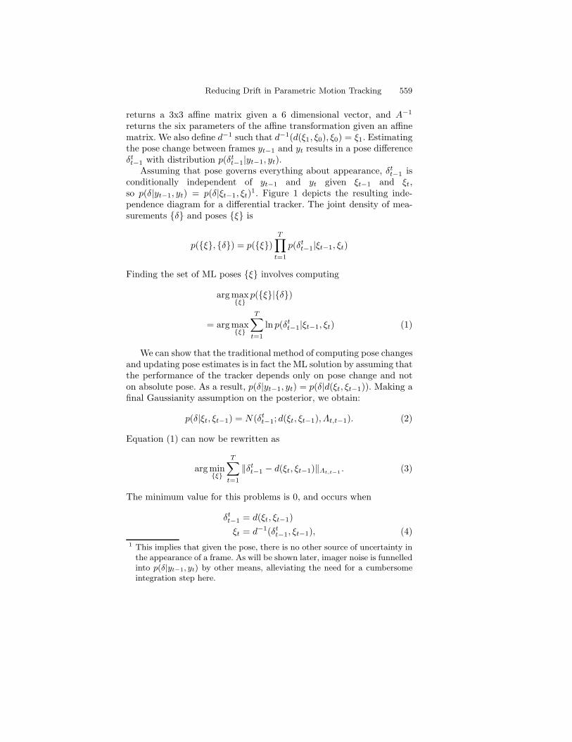
returns the six parameters of the affine transformation given an affinematrix. We also define d−1 such that d−1(d(ξ1, ξ0), ξ0) = ξ1. Estimatingthe pose change between frames yt−1 and yt results in a pose differenceδtt−1 with distribution p(δt

t−1|yt−1, yt).Assuming that pose governs everything about appearance, δt

t−1 isconditionally independent of yt−1 and yt given ξt−1 and ξt,so p(δ|yt−1, yt) = p(δ|ξt−1, ξt)1. Figure 1 depicts the resulting inde-pendence diagram for a differential tracker. The joint density of mea-surements {δ} and poses {ξ} is

p({ξ}, {δ}) = p({ξ})T∏

t=1

p(δtt−1|ξt−1, ξt)

Finding the set of ML poses {ξ} involves computing

arg max{ξ}

p({ξ}|{δ})

= arg max{ξ}

T∑t=1

ln p(δtt−1|ξt−1, ξt) (1)

We can show that the traditional method of computing pose changesand updating pose estimates is in fact the ML solution by assuming thatthe performance of the tracker depends only on pose change and noton absolute pose. As a result, p(δ|yt−1, yt) = p(δ|d(ξt, ξt−1)). Making afinal Gaussianity assumption on the posterior, we obtain:

p(δ|ξt, ξt−1) = N(δtt−1; d(ξt, ξt−1), Λt,t−1). (2)

Equation (1) can now be rewritten as

arg min{ξ}

T∑t=1

‖δtt−1 − d(ξt, ξt−1)‖Λt,t−1 . (3)

The minimum value for this problems is 0, and occurs when

δtt−1 = d(ξt, ξt−1)ξt = d−1(δt

t−1, ξt−1), (4)1 This implies that given the pose, there is no other source of uncertainty in

the appearance of a frame. As will be shown later, imager noise is funnelledinto p(δ|yt−1, yt) by other means, alleviating the need for a cumbersomeintegration step here.


Fig. 1. Independence diagram for a simple pose tracker. The tracker measurespose differences {δ} between adjacent frames.

confirming that the traditional update equation does indeed maximizelikelihood given the simplifying assumptions we’ve made. Note thatΛt,t−1 drops out of the optimization, and so it is not necessary to com-pute the error in pose changes.

2.2 Using multiple base frames to reduce drift

To improve pose estimation, we invoke two principal insights:

1. When the trajectory comes close to crossing itself (ie, ξt ≈ ξs, t >s), tracking should be performed between frames yt and ys as well.

2. Information about the pose of future frames can be used to adjustthe pose estimate of past frames.

Proposition 1) provides redundant reliable information which allowsus to better estimate pose. Proposition 2) is appealing since returningnear a previously visited point can disambiguate measurements if in-formation from the future is allowed to affect the past. Hence, in figure2, we would do well to compute a pose change estimate between yt andall frames that lie in the shaded region, and allow these measurementsto influence the pose of frames y1 · · · yt.

We augment the measurement model laid out in the previous sec-tion to incorporate these additional measurements. To improve perfor-mance, we can also incorporate knowledge about the dynamics of thepose parameters. Figure 3 shows how to update the graphical model of


y0

y1

y2

y3

y4

y5

yt

y�t-1�

yt-2

Fig. 2. When estimating the pose of frame yt, we should take into accountthe pose change between yt and yt−1 as well as all other frames which are inthe shaded region.

Fig. 3. The measurement model when multiple base frames are used. A dy-namical model for pose change is also added (horizontal arrows).


the differential tracker to incorporate the added information. The jointof the poses and observations becomes

p({ξ}, {δ}) = p(ξ0)T∏

t=1

p(ξt|ξt−1)∏

(f,g)∈ D

p(δgf |ξf , ξg)

where D is the set of pairs of frames between which we have calculatedthe pose change. Using the Gaussian uncertainty model of (2), the MLposes are

arg min{ξ}

∑(f,g)∈ D

‖δtt−1 − d(ξt, ξt−1)‖Λt,t−1

+T∑

t=1

‖d(ξt, ξt−1)‖Λd(5)

where we have assumed that the pose dynamics are Brownian withcovariance Λd. The optimization problem can be thought of as relaxinga spring system where the natural length of a spring between nodes ξf

and ξg is δgf and its stiffness is Λ−1

f,g.Unlike the minimization problem of the traditional tracker, we now

need to know Λf,g. An approximation to Λf,g is derived in the followingtwo sections.

2.3 Estimating pose change

The simplest pose change tracker computes the maximum likelihoodpose difference δt

t−1 by assuming that yt can be warped back to yt−1.Camera noise and any change in appearance that is not modelled bywarping is modelled with identically distributed and independent Gaus-sian noise of unspecified variance added to every pixel. The generativemodel of yt−1 is then:

yt−1(x) = yt(x − u(x; δtt−1)) + w(x)

p(yt−1(x)|yt(x), δtt−1) = N (yt−1(x); (6)

yt(x − u(x; δtt−1)), σ

2w)

where w(x) is Gaussian and white over space and time, and has con-stant variance σ2

w over the image. N (x; µ, σ2) is a Gaussian distributionwith means µ and variance σ2. u(x; δ) is the warping function: it is usedto displace a pixel at location x to location x + u(x; δ) in the target


image. The ML estimate, δ, maximizes the posterior p(δ|yt, yt−1). Thisis equivalent to minimizing a sum-of-squared error function over δ:

δ = argmaxδ

p(δ|yt, yt−1) (7)

= argminδ

∑x

[yt−1(x) − yt(x − u(x; δ))]2

This is the traditional least squares formulation for tracking, derivedin a probabilistic framework. Various total-least squares formulationswhich allow yt to be noisy as well have been proposed [13, 8]. We havedemonstrated that pose change estimation computes the mode of thedistribution p(δ|yt, yt−1). To fully qualify this distribution, we still needto compute its covariance Λt,t−1.

2.4 Uncertainty in motion estimates

Probabilistic methods for computing uncertainty in optical flow havebeen proposed in [12, 8]. We approximate the posterior p(δ|yt, yt−1) byfitting a Gaussian distribution at the mode δ computed by the pose esti-mator. The derivation is based on the approximation made in Laplace’smethod (see [6] for a note on the subject).

Using Bayes rule, we can rewrite the log-posterior:

log p(δ|yt, yt−1) = log p(yt−1|δ, yt) (8)+ log p(δ|yt) − log p(yt−1|yt)

Since δ is taken to be the ML estimate, the first derivative of (8) van-ishes at δ. Assuming uniform p(δ|yt) (this is the case if p(δ) is itselfuniform, since we can glean nothing about future poses from a singleimage), the Hessian of (8) becomes

H =∂2

∂δ2log p(δ|yt, yt−1) =

∂2

∂δ2log p(yt−1|yt, δ)

The Taylor expansion of (8) about its mode is therefore:

log p(δ|yt, yt−1) ≈ log p(δ|yt, yt−1)

+12∆δT ∂2

∂δ2log p(yt−1|yt, δ)∆δ

+ H.O.T.,

where ∆δ = δ − δ. Dropping high order terms and exponentiating, weobtain a Gaussian approximation to the posterior:

p(δ|yt, yt−1) ≈ α exp(

12(δ − δ)TH(δ − δ)

)


This Gaussian has mean δ as expected, and its variance is Λt,t−1 =−H−1. In this case, H is the Hessian of the log of

p(yt−1|yt, δ) =∏x

p(wt(x))

=∏x

N(yt−1(x); yt(x − u(x; δ)), σ2w),

which is found to be

H =1

σ2w

∑x

∂u

∂δ

T

(yt−1∇2xyt−1 −∇yt∇yT

t )∂u

∂δ,

where ˆyt−1 = yt(x − u(x; δ)) is the reconstructed yt−1 and yt−1(x) =yt−1(x) − yt−1(x) is the reconstruction residual2. Since in practice thereconstruction error is small, we can further approximate H by:

H = − 1σ2

w

∑x

∂u

∂δ

T

∇yt−1(x)[∇yt−1(x)]T )∂u

∂δ,

Finally, σ2w can be estimated as

σ2w =

1N

∑x

[yt−1(x) − yt(x − u(x; δ))]2. (9)

Our final estimate of the variance of p(δ|yt, yt−1) is:

Λt,t−1 = σ2w

[∑x

∂u

∂δ

T

∇yt−1(x)∇yt−1(x)T ∂u

∂δ

]−1

.

This expression has an intuitive interpretation which makes it suitableas an approximation of the posterior covariance. σ2

w can be interpretedas the RMS reconstruction error after warping according to the recov-ered pose change. H can be interpreted as the average sensitivity ofeach component of δ, weighted by the strength of the features in theimage. This is because ∇y(x)∇y(x)T represents the strength of a fea-ture at location x (see [10]), and ∂u

∂δ (x; δ) is a measure of the sensitivityof δ at various points in the image.

To illustrate this point, we compute the sensitivity of a transla-tional and an affine tracker. In the translational case, u(x; δ) = δ. So2 In deriving this expression, we have assumed that ∂2u/∂δ2 = 0. ie, u is

linear wrt δ.


∂∂δ u(x; δ) = I. The covariance becomes

Λtranslation = σ2w

[∑x

∇y∇yT

]−1

, (10)

which is just the reconstruction error weighted by a measure of howtextured the image is.

In the case of an affine tracker, the partial of u is:

∂

∂δu(x; δ) =

[x y 1 0 0 00 0 0 x y 1

].

If we set ∇yt−1(x)∇yt−1(x)T = I, effectively assigning to all points thesame feature properties, the covariance becomes

Λaffine = σ2w

∑

x

x2 xy xxy y2 yx y 1

0

0x2 xy xxy y2 yx y 1

−1

.

According to this expression, points away from the center of the coor-dinate system reduce the uncertainty in the multiplicative portion ofthe affine transformation more than the central points. In addition allpoints contribute equally to the translation parameters. Both observa-tions are consistent with our expectation.

3 Results: a simple 2D tracker

We first show results when tracking the position of an aperture movingover an image. ξt represents the current pixel location of the apertureand yt denotes the image captured through the aperture. Since ξ onlyparametrizes translation, a simple motion model with u(x; δ) = δ isadequate. Figure 4 shows the pose estimates from a differential trackerwhich finds pose changes by minimizing (8) using gradient descent. Theupdate is according to (4) and is additive.

The algorithm estimates the pose change between consecutive 50x50pixel windows which translate by an average of 5.6 pixels each stepalong a spiral path. The average error in estimating δ is around 0.66pixels, which after 626 iterations, results in approximately 55 pixels ofdrift.


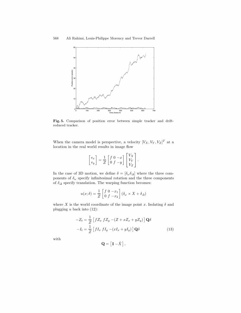
To measure the uncertainty of the pose change estimator, we usedthe pose covariance from equation (10). Figure 4 displays tracking per-formance on the same aperture trajectory. The previous frame wasalways used as an anchor frame, along with the 3 past frames whichwere closest in pose to the previous frame. In 626 frames, tracking driftsby at most 2.44 pixels and is off by 0.11 pixels at frame 623. Figure 5compares the pose error of the two trackers over time. The the drift-reduced tracker stops accumulating error after about 50 frames, whilethe unenhanced tracker continues drifting.

To find the poses which maximize equation (5), we computed thederivatives of the log-likelihood with respect to each pose:

0 =∂

∂ξip({δ}|{ξ})

= −∑

(f=i,g)∈D

Λi,g(δgi − ξi + ξg)

+∑

(f,g=i)∈ D

Λf,i(δif − ξf + ξi) (11)

Equation (11) is a sparse linear system in terms of the poses. Given afixed value for ξ0, this system can be solved very efficiently (Matlab’sbackslash operator, which uses simple Gaussian elimination solves theabove 626 frame problem in less than a second).

4 Stabilized 3D tracking

Our method can also be applied to 3D tracking. We show results usinga rigid motion tracker with integrated intensity and depth constraints,but our method is applicable to any parametric motion formulation,with or without depth constraints.

Depth constraints have been shown to increase the accuracy ofgradient-based rigid motion tracking [3]. A depth constancy constraintanalogous to the traditional brightness constancy constraint can bederived and yields:

−It =[Ix Iy

]u(x; δ)

−Zt =[Zx Zy

]u(x; δ) − Vz(x, δ) (12)

where Ix, Zx, etc, are the partials of yt or yt−1. Together, these equa-tions constrain the local motion δt

t−1 by using the image gradients.


100 150 200 250 300

100

120

140

160

180

200

220

240

260

100 150 200 250 300

100

120

140

160

180

200

220

240

260

Fig. 4. Estimates of the position of a 50x50 pixel aperture as it follows aspiral path on the image. The position estimate is based solely on the im-age acquired through the aperture. Top: traditional tracker. The estimatedtrajectory (solid) terminates (marked by ’×’) with more than 55 pixels oferror relative to ground truth (dotted). Bottom: drift-reduced tracker, usingat most 4 past frames. The estimated trajectory ends less than 1 pixels fromthe ground truth.


0 100 200 300 400 500 600 7000

10

20

30

40

50

60

Pos

ition

err

or (

pixe

ls)

Time (frame #)

Fig. 5. Comparison of position error between simple tracker and drift-reduced tracker.

When the camera model is perspective, a velocity [VX , VY , VZ ]T at alocation in the real world results in image flow

[vx

vy

]=

1Z

[f 0 −x0 f −y

] VX

VY

VZ

.

In the case of 3D motion, we define δ = [δωδ∆] where the three com-ponents of δω specify infinitesimal rotation and the three componentsof δ∆ specify translation. The warping function becomes:

u(x; δ) =1Z

[f 0 −x1

0 f −x2

](δω × X + δ∆)

where X is the world coordinate of the image point x. Isolating δ andplugging u back into (12):

−Zt =1Z

[fZx fZy −(Z + xZx + yZy)

]Qδ

−It =1Z

[fIx fIy −(xIx + yIy)

]Qδ (13)

withQ =

[I −X

],


where X is the 3x3 skew symmetric matrix formed by the real-worldcoordinates corresponding to x and I is the 3x3 identity matrix. Thesystem of equation (13) is linear and highly overconstrained and canbe easily solved for δ.

For infinitesimal 3D updates, d(ξ1, ξ0) should be the real eigenvectorof eξ1e−ξ0 [7], but we have found that d(ξ1, ξ0) = ξ1 − ξ0 is adequate inpractice. Drift reduction then consisted in solving equation (11) usinga sparse linear system solver.

4.1 Results: 6-DOF head tracker

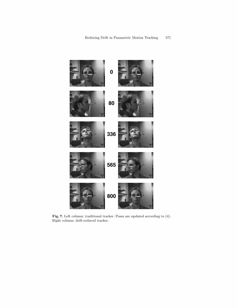
We demonstrate the performance of the drift reduction algorithm onthis 3D tracker. Figure 6 describes the direction of a head as the subjectlooks around the room. The nose moves by at most 20 cm throughoutthe sequence and the head yaws by up to 80 degrees in each direc-tion and pitches by up to a total of 55 degrees. The sequence is 800frames long and corresponds to about 1.2 minutes of video. The facewas segmented from the background using the depth information only.Pose changes were computed using the combined constraints of (13).As shown in figure 7, after about 600 frames, the traditional trackerhas accumulated noticeable drift in its estimate of rotation, whereas thedrift-reduced tracker shows the pointer on the subject’s nose wheneverhe returns to a near-frontal pose. Only appearance was used in findingsuitable anchor frames. Figure 8 plots the index of anchor frames usedfor each frame. The protrusions from the diagonal line are produced asthe subject returns from a rotation. Note that the first frame is neverreused. The robustness is entirely due to recovering from drift accumu-lated during each rotation by using frames observed while going intothe rotation.

4.2 Results: egomotion

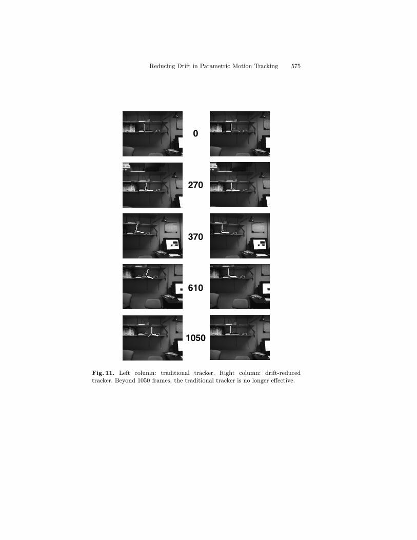
The sequence summarized in figure 9 demonstrates that the drift re-duced tracker can also be used for computing ego-motion. The task isto hold the pointer in the same location relative to the real world asthe camera scans the room. Between frames 400 and 600, almost noneof the original scene is visible. By frame 610, the drift-reduced trackershows significant improvement over the traditional tracker, despite thedearth of back frames before frame 630. The superior performance inthe early frames demonstrates the benefits of the batch/non-causal na-ture of the drift-reduction algorithm and of allowing information in thefuture influence the past. By frame 1050 the unenhanced tracker has


0 100 200 300 400 500 600 700 800-1.5

-1

-0.5

0

0.5

1

1.5PitchYaw Roll

80 480 33622080

565480

405

660 750

0

800

80

220

336

405480

565

660

750

Fig. 6. The sequence is 1.2 minutes long. The subject looks in all directions,by up to 80 degrees from frontal in some directions. The sequence was cap-tured at ∼11 fps. The graph above provides an intuitive feel for the relativemagnitude of the rotations. It plots δω over time.


0

336

565

800

80

Fig. 7. Left column: traditional tracker. Poses are updated according to (4).Right column: drift-reduced tracker.


0 100 200 300 400 500 600 700 800 9000

100

200

300

400

500

600

700

800

900

Current image

Mat

ched

imag

es

Fig. 8. Anchor frames used by drift-reduced tracker. Each frame on the hori-zontal axis is matched by appearance with 3 previous frame. The protrusionsshow that as the subject returns from a rotation, frames on the way into therotation are used as anchor.

drifted far enough that all subsequent pose changes throw it even fur-ther off track. Figure 10 shows a quantitive version of the results. After600 frames, the traditional tracker starts to accumulate considerabledrift. During the same period, the drift-reduced tracker keeps track ofthe real movement by using information prom similar previous framesas shown in figure 12.


230 450

930540 800

0

0

230

450

540

800

930

Fig. 9. The camera begins panning from the center dot, in the direction ofthe arrow. The dashed path marks the approximate trajectory of the centerof the camera (drawn by hand). Only the interior of the black rectangle isvisible to the camera (approximate), so that the intial pose is completely outof view between frames 420 and 530.


0 200 400 600 800 1000 1200−400

−200

0

200

400

600

800

1000

0 200 400 600 800 1000 1200−500

0

500

1000

1500

2000

Traditional Drift−reduced

Fig. 10. Top: Horizontal translation. Bottom: Vertical Translation. The tra-ditional tracker exhibits continual drift with respect to the drift-reducedtracker.


0

370

610

1050

270

Fig. 11. Left column: traditional tracker. Right column: drift-reducedtracker. Beyond 1050 frames, the traditional tracker is no longer effective.


0 200 400 600 800 1000 12000

200

400

600

800

1000

1200

Current image

Mat

ched

imag

es

Fig. 12. Anchor frames used by drift-reduced tracker. Previously visitedposes are used effectively (eg, frames 300, 700, 1020).


5 Conclusion

We have developed a framework for stabilizing parametric motion track-ers in closed environments. Our method measures pose change betweenframes which are similar in pose and appearance, and uses these mea-surements to compute robust pose estimates. This improves stabil-ity since additional pose change measurements provide robustness andground the tracking against commonly revisited sites. We derived anuncertainty model for motion estimation and used it to frame the prob-lem of incorporating these additional measurements into a non-causalestimation framework. We demonstrated the benefits of using multiplebase frames in our maximum likelihood framework on a synthetic 2Dmotion tracking problem and on 3D ego-motion computation and poseestimation.

6 Acknowledgement

Many thanks to Tom Minka for suggesting the Hessian approximationused in section 2.4.

References

1. S. Birchfield. Elliptical head tracking using intensity gradients and colorhistograms. In CVPR, pages 232–237, 1998.

2. G. Hager and P. Belhumeur. Efficient region tracking with parametricmodels of geometry and illumination. PAMI, 20(10):1025–1039, 1998.

3. M. Harville, A. Rahimi, T. Darrell, G. Gordon, and J. Woodfill. 3d posetracking with linear depth and brightness constraints. In Proceedings ofCVPR 99, pages 206–213, Corfu, Greece, 1999.

4. T. Jebara and A. Pentland. Parametrized structure from motion for 3dadaptive feedback tracking of faces. In CVPR, 1997.

5. M. LaCascia, S. Sclaroff, and V. Athitsos. Fast, reliable head track-ing under varying illumination: An approach based on registration oftextured-mapped 3d models. PAMI, 22(4):322–336, April 2000.

6. T.P. Minka. Using lower bounds to approx-imate integrals. Technical report, Media Lab,http://www.media.mit.edu/˜tpminka/papers/rem.html, 2001.

7. Richard M. Murray, Zexiang Li, and S. Shankar Sastry. A MathematicalIntroduction to Robotic Manipulation. CRC Press, 1994.

8. O. Nestares, D.J. Fleet, and D.J. Heeger. Likelihood functions and con-fidence bounds for total-least-squares problems. In CVPR, 2000.

9. N. Oliver, A. Pentland, and F. Berard. Lafter: Lips and face real timetracker. In Computer Vision and Patt. Recog., 1997.


10. J. Shi and C. Tomasi. Good features to track. In CVPR94, pages 593–600, 1994.

11. H.-Y. Shum and R. Szeliski. Construction of panoramic mosaics withglobal and local alignment. In IJCV, pages 101–130, February 2000.

12. E.P. Simoncelli, E.H. Adelson, and D.J. Heeger. Probability distributionsof optical flow. In CVPR91, pages 310–315, 1991.

13. J. Weber and J. Malik. Robust computation of optical flow in a multi-scale differential framework. IJCV, 14(1):67–81, 1995.

14. C. Wren and A. Pentland. Dynamic models of human motion. In Pro-ceedings of Face and Gestures, 1998.

Reducing Drift in Parametric Motion Tracking

Documents

Transcript of Reducing Drift in Parametric Motion Tracking