Institut fur Computergraphik undAlgorithmen

Technische Universitat Wien

Karlsplatz 13/186/2A-1040 Wien

AUSTRIA

Tel: +43 (1) 58801-18601Fax: +43 (1) 58801-18698

Institute of Computer Graphics andAlgorithms

Vienna University of Technology

email:technical-report@cg.tuwien.ac.at

other services:http://www.cg.tuwien.ac.at/

ftp://ftp.cg.tuwien.ac.at/

Combined Rendering of Polarization andFluorescence Effects

Alexander Wilkie, Robert F. Tobler, Werner Purgathofer

TR-186-2-01-11

April 2001

Abstract

We propose a practicable way to include both polarization and fluorescence effects in arendering system at the same time. Previous research in this direction only demonstratedsupport for either one of these phenomena; using both effects simultaneously was so farnot possible, mainly because the techniques for the treatment of polarized light were com-plicated and required rendering systems written specifically for this task.The key improvement over previous work is that we use a different, more easily handledformalism for the description of polarization state, which also enables us to include flu-orescence effects in a natural fashion. Moreover, all of our proposals are straightforwardextensions to a conventional spectral rendering system.

Keywords: polarization, fluorescence, predictive rendering

1 Introduction

For the purposes of truly predictive photorealistic rendering it is essential that no effectwhich contributes to the interaction of light with a scene is neglected. Most aspects ofobject appearance can be accounted for by using just the laws of geometric optics, com-paratively simple descriptions of surface reflectivity, tristimulus representations of colourand light, and can nowadays be computed very efficiently through a variety of commonrendering algorithms. However, several physical effects, namely fluorescence, diffraction,dispersion and polarization, are still rarely – if at all – supported by contemporary renderingsoftware.

1.1 Polarization

Polarization has received particularly little attention because – while of course being es-sential for specially contrived setups that e.g. contain polarizing filters – it seemingly doesnot contribute very prominent effects to the appearance of an average scene. This mis-conception is in part fostered by the fact that the human eye is normally not capable ofdistinguishing polarized from unpolarized light1.One of the main areas where it in fact does make a substantial difference are outdoor scenes;this is due to the usually quite strong polarization of skylight, as one can find documentedin G. P. Konnen’s book [6] about polarized light in nature. But since such scenes are cur-rently still problematical for photorealistic renderers for a number of other, more obviousreasons (e.g. scene complexity and related global illumination issues), this has not beengiven a lot of attention yet. Other known effects which depend on polarization support arecertain darkening or discolourization patterns in metal objects and their reflections, and thedarkening of certain facets in transparent objects such as crystals.

1.2 Fluorescence

Some of the reasons for the small amount of work fluorescence has received are differentfrom those which have made polarization a fringe topic. Firstly, although it causes veryprominent effects, these can also be faked comparatively easily through custom shaders ata fraction of the effort involved in actually simulating the real process. Secondly, measure-ments of fluorescent pigments are very hard to obtain, virtually no publicly accessible dataof this kind exists, and designing such spectra by hand is tedious. The third main reasonis shared between fluorescence and polarization: they ought to be done using a spectralrendering system, which still rank as comparatively exotic and expensive to use.

2 Background

In this section we discuss three topics: we give a brief overview of the physics behind thephenomena of polarized light and of fluorescence, and we recapitulate the workings of aparticular ubiquitous raytracing acceleration technique, since this has implications on howpolarization support ought to be implemented in a rendering system.

1Contrary to common belief trained observers can distinguish polarized from unpolarized light with the nakedeye. Named after its discoverer, the effect is known as Haidinger’s brush and is described by Minnaert in his bookabout light in outdoor surroundings [7].

2.1 Polarized Light

While for a large number of purposes it is sufficient to describe light as an electromagneticwave of a certain frequency that travels linearly through space as a discrete ray (or a set ofsuch rays), closer experimental examination reveals that such a wavetrain also oscillates ina plane perpendicular to its propagation. The exact description of this phenomenon requiresmore than just the notion of radiant intensity, which the conventional representation of lightprovides.The nature of this oscillation can be seen from the microscopic description of polarization,which closely follows that given by Shumaker [11]. We consider a single steadily radiatingoscillator (the light source) at a distant point of the negative Z–axis, and imagine that wecan record the electric field2 present at the origin due to this oscillator. Except at distancesfrom the light source of a few wavelengths or less, the Z component of the electric fieldwill be negligible and the field will lie in the X–Y plane. The X and Y field componentswill be of the form

Ex� Vx

� � 2π � ν � t � δx ���V � m � 1 �Ey

� Vy� � 2π � ν � t � δy � (1)

where Vx and Vy are the amplitudes �V � m � 1 � , ν is the frequency �Hz � , δx and δy are thephases � rad� of the electromagnetic wavetrain, and t is the time � s � . Figure 1 illustrates howthis electric field vector E changes over time for four typical configurations.

� ����

�

�Fig. 1. Left: Four examples of the patterns traced out by the tip of the electric field vector in the X–Yplane: a) shows light which is linearly polarized in the vertical direction; the horizontal componentEx is always zero. b) is a more general version of linear polarization where the axis of polarization istilted by an angle of α from horizontal, and c) shows right circular polarized light. The fourth exampled) shows elliptically polarized light, which is the general case of equation (1). (Image redrawnfrom Shumaker [11]) Right: Geometry of a ray–surface intersection with an optically smooth phaseboundary between two substances, as described by the equation set (2). A transmitted ray T onlyoccurs in when two dieelectric media interface; in this case, all energy that is not reflected is refracted,i.e. T � I � R. The E–vectors for the transmitted ray Et � and Et � have been omitted for better pictureclarity. The � E ��� E ��� components here correspond to the � x � y � components in the drawing on the left.

Causes of Light Polarization. Apart from skylight, it is comparatively rare for light tobe emitted in polarized form. In most cases, polarized light is the result of interaction with

2The electric and magnetic field vectors are perpendicular to each other and to the propagation of the radiation.The discussion could equally well be based on the magnetic field; which of the two is used is not important.

transmitting media or surfaces. The correct simulation of such processes is at the core ofpredictive rendering, so a short overview of this topic recommends itself.The simplest case is that of light interacting with an optically smooth surface. This scenariocan be adequately described by the Fresnel equations, which are solutions to Maxwell’swave equations for light wavefronts. They have been used in computer graphics at leastsince Cook and Torrance proposed their famous reflectance model [2], and most applica-tions use them in a form which is simplified in one way or another.

Fresnel Terms. In their full form (the derivation of which can e.g. be found in [12]), theyconsist of two pairs of equations. According to the reflection geometry in figure 1, the firstpair determines the proportion of incident light which is reflected separately for the x andy components of the incident wavetrain. This relationship is commonly known, and can befound in numerous computer graphics textbooks.The second pair, which is much harder to find in computer graphics literature, descibes theretardance that the incident light is subjected to, which is the relative phase shift that thevertical and horizontal components of the wavetrain undergo during reflection. In figure2 we show the results for two typical materials: one conductor, a class of materials whichhas a complex index of refraction and is always opaque, and one dieelectric, which in pureform is usually transparent, and has a real–valued index of refraction.We quote the Fresnel equations for a dieelectric–complex interface. This is the generalcase, since only one of two media at an interface can be conductive (and hence opaque),and a dieelectric–dieelectric interface with two real–valued indices of refraction can alsobe described by this formalism.

F� � θ � η � � a2 � b2 � 2acosθ � cos2 θa2 � b2 � 2acosθ � cos2 θ

F� � θ � η � � a2 � b2 � 2asinθ tanθ � sin2 θ tan2 θa2 � b2 � 2asinθ tanθ � sin2 θ tan2 θ

F� � θ � η �tanδ � � 2cosθ

cos2 θ � a2 � b2

tanδ � � 2bcosθ � � n2 � k2 � b � 2nka ��n2 � k2 � 2 cos2 θ � a2 � b2

with

2a2 � � �n2 � k2 � sin2 θ � 2 � 4n2k2 � n2 � k2 � sin2 θ

2b2 � � �n2 � k2 � sin2 θ � 2 � 4n2k2 � n2 � k2 � sin2 θ

(2)

F� is the reflectance component parallel to the plane of incidence, and F� that normal toit. Under the assumption that one is only interested in the radiant intensity of the reflectedlight, this can be simplified to the commonly used average reflectance Faverage

� �F� �

F� ��� 2. δ � and δ � are the retardance factors of the two wavetrain components.

2.2 Fluorescence

While the polarization of light at a phase boundary is a comparatively macroscopic phe-nomenon, fluorescence is caused by processes within the pigment molecules that are re-sponsible for the colour of an object. Due to both lack of space, and the fact that an actual

0 30 60 90

0.5

0.0

1.0

Copper

Lead Crystal

Reflectivity

30 60 90

� 90

� 45

45

0

90 Retardance

Copper

Lead Crystal

Fig. 2. Fresnel reflectivities F � , F � and Faverage (dashed lines), as well as parallel and perpendicularretardance values for copper (red) and lead crystal (blue) at 560nm. As a conductor, copper has acomplex index of refraction, does not polarize incident light very strongly at Brewster’s angle andexhibits a gradual shift of retardance over the enitre range of incident angles. For lead crystal, withits real–valued index of refraction of about 1.9, total polarization of incident light occurs at about62

�

. Above this angle, no change in the phase relation of incident light occurs (both retardancecomponents are at � 90

�

), while below Brewster’s angle a phase difference of 180�

is introduced.

explanation of these processes is not necessary to properly implement support for it in arendering system, we will not go into details about its causes.The results of the phenomenon – which are what we try to simulate – are quite straightfor-ward to describe: the characteristic property of fluorescent materials is that they re–emitportions of the incident light at different, lower wavelengths within an extremely short time(typically 10 � 8 seconds).Instead of the reflectance spectra used for normal pigments, describing such a material re-quires knowledge of its re–radiation matrix, which encodes the energy transfer betweendifferent wavelengths. Such bispectral reflectance measurements are rather hard to comeby; while “normal” spectrophotometers are becoming more and more common, the bis-pectral versions of such devices are by comparison very rare and in an experimental stage.Figure 3 shows three visualizations of a sample bispectral reflectance dataset.Manual design of such re–readiation matrices is much harder than explicit derivation ofreflection spectra; while the latter is already not particularly easy, their effect is by com-parison still quite predictable. Also, it is easy to maintain the energy balance of normalreflection spectra by ensuring that no component is greater than one; for a re–readiationmatrix this translates to the more difficult condition that the integral over the area must notexceed one.

2.3 Raytracing with Adaptive Tree–Depth Control

Historically, the introduction of recursive raytracing by Whitted [15] can be considered oneof the major breakthroughs in the use of ray–based image synthesis methods. Subsequentwork addressed performance optimization of such renderers; one key contribution in thisarea was the proposal of Hall and Greenberg [4] to adaptively prune the tree of recursive in-tersections for a given sample point, a technique which is in such widespread use nowadaysthat it is usually taken for granted.Instead of recursively tracing reflections to a given recursion depth and simply adding thecontributions of all successive ray intersections, they suggested to consider the possiblemaximum contribution of child rays (the so–called ray weight) to a sample point, and to

300 380 500 600 700 780

380

500

600

700

780300 380 500 600 700 780

380

500

600

700

780

500 600 700

0.2

0.4

0.6

0.8

1

1.2

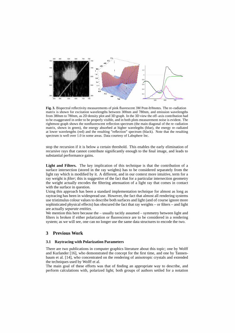
Fig. 3. Bispectral reflectivity measurements of pink fluorescent 3M Post-It® notes. The re–radiationmatrix is shown for excitation wavelengths between 300nm and 780nm, and emission wavelengthsfrom 380nm to 780nm, as 2D density plot and 3D graph. In the 3D view the off–axis contribution hadto be exaggerated in order to be properly visible, and in both plots measurement noise is evident. Therightmost graph shows the nonfluorescent reflection spectrum (the main diagonal of the re–radiationmatrix, shown in green), the energy absorbed at higher wavelegths (blue), the energy re–radiatedat lower wavelengths (red) and the resulting ”reflection” spectrum (black). Note that the resultingspectrum is well over 1.0 in some areas. Data courtesy of Labsphere Inc.

stop the recursion if it is below a certain threshold. This enables the early elimination ofrecursive rays that cannot contribute significantly enough to the final image, and leads tosubstantial performance gains.

Light and Filters. The key implication of this technique is that the contribution of asurface intersection (stored in the ray weights) has to be considered separately from thelight ray which is modified by it. A different, and in our context more intuitive, term for aray weight is filter; this is suggestive of the fact that for a particular intersection geometrythe weight actually encodes the filtering attenuation of a light ray that comes in contactwith the surface in question.Using this approach has been a standard implementation technique for almost as long asraytracing has been in widespread use. However, the fact that almost all rendering systemsuse tristimulus colour values to describe both surfaces and light (and of course ignore moresophisticated physical effects) has obscured the fact that ray weights – or filters – and lightare actually separate entities.We mention this here because the – usually tacitly assumed – symmetry between light andfilters is broken if either polarization or fluorescence are to be considered in a renderingsystem; as we will see, one can no longer use the same data structures to encode the two.

3 Previous Work

3.1 Raytracing with Polarization Parameters

There are two publications in computer graphics literature about this topic; one by Wolffand Kurlander [16], who demonstrated the concept for the first time, and one by Tannen-baum et al. [14], who concentrated on the rendering of anisotropic crystals and extendedthe techniques used by Wolff et al.The main goal of these efforts was that of finding an appropriate way to describe, andperform calculations with, polarized light; both groups of authors settled for a notation

suggested by standard reference texts from physics literature.

Coherency Matrices. The formalism to describe polarized light used by both Wolff andTannenbaum is that of coherency matrices (CM for short); this technique was introduced byBorn and Wolf [1]. Similar to the discussion in section 2.1, one considers a monochromaticwave propagating along the positive Z–axis, and treats the E–field vector as consistingof two orthogonal components in X and Y directions. The phase relationships betweenthe two can exhibit anything between full correlation (fully coherent or polarized light)to totally uncorrelated behaviour (incoherent or unpolarized light). As derived in detailby Tannenbaum et al. [14], the coherency state of such a monochromatic wave can beexpressed in a matrix J of the form

J � �Jxx JxyJyx Jyy � � ���

ExE �x � �ExE �y ��

EyE �x � �EyE �y � �

where Ex and Ey are the time average of the E–field vectors for the X and Y directions,respectively, and E �x denotes the complex conjugate of Ex. The main diagonal elements– Jxx and Jyy – are real valued, and the trace T

�J � of the matrix represents the total light

radiation of the wave, while the complex conjugates Jxy and Jyx represent the correlationof the X and Y components of E. For fully polarized light, these components are fullycorrelated and � J � vanishes.It is worth noting that coherency matrices – while they might seem rather different at firstglance – encode the same information as equation (1). Born and Wolf [1] also discuss howone can compute the elements of a coherency matrix from actual irradiance measurements,which is an important point if one wants to eventually validate computer graphics modelsthat use polarization in their calculations.

Coherency Matrix Modifiers. Besides being able to describe a ray of light, it is alsonecessary to process the interaction of light with a medium, as outlined in section 2.3. Suchfiltering operations on polarized light described by a coherency matrix can be performedby using coherency matrix modifiers, or CMM. Tannenbaum et al. brought this approach,which was originally introduced by Parrent et al. [8], to the computer graphics world foruse in their rendering system.CMMs have the form of a real–valued 4 � 4 matrix. If all participating elements havethe same reference coordinate system, such matrices can be applied to a given coherencematrix J in the sequence of Jp

� MpJM †p , where M †

p signifies the conjugate transpose ofMp. If the modifier and the coherency matrix are not in the same coordinate system, anappropriate transformation – as discussed in section 2.3 of Tannenbaum et al. [14] – has tobe applied first.

3.2 Reflection Models which take Polarization into Account

Apart from the case of perfect specular reflection and refraction, which is already ade-quately covered by the Fresnel terms discussed in section 2.1 and the modified Cook–Torrance model used by Wolff et al., only one other surface model proposed so far, namelythat of He et al. [5], attempts to consider polarization effects. As could be inferred fromthe results section of this paper, the high complexity of their surface model apparently ledthe authors to only implement a simpler, non–polarizing version in practice, and to containthemselves with just providing the theoretical derivation of the polarization–aware modelin the text.

3.3 Rendering of Fluorescence Effects

So far Glassner has apparently been the only graphics researcher who investigated the ren-dering of fluorescence phenomena [3]. The main focus of his work was centered aroundthe proper formulation of the rendering equation in the presence of phosphorescence andfluorescence, and he provided striking results generated with a modified version of thepublic domain raytracer rayshade. Sadly, this work was not followed up, nor was the mod-ified version of rayshade made public. Also, we are not aware of any work that aims atconsidering the inclusion of fluorescence effects in sophisticated reflectance models.

4 A Combined Renderer

We first introduce an alternative notation that can be used for polarization support, and thenshow how this formalism can easily be combined with fluorescence support.

4.1 Alternative Polarization Support

A description for polarized radiation which due to its simpler mathematical characteristicsisis better suited for use in raytracing–based rendering systems is that of Stokes parameters.This description, while equivalent to coherency matrices, has the advantage of using onlyreal–valued terms to describe all polarization states of optical radiation, and has an – alsononcomplex – corresponding description of ray weights in the form of Muller matrices[11].It has to be kept in mind that – similar to coherency matrices – both Stokes parametersand Muller matrices are meaningful only when considered within their own local referenceframe; the main effect of this is that in a rendering system not only light, but also filtersare oriented and have to store an appropriate reference in some way. However, for the sakebrevity this spatial dependency is omitted in our following discussion except in the sectionabout matrix realignment.

Stokes Parameters. Apart from coherency matrices, the polarization state of an elec-tromagnetic wave of a given frequency can also be described in several other ways. Threereal–valued parameters are required to describe a general polarization ellipse, but the Stokesvector notation defined by

En � 0� κ

�V 2

x � V2y � �W � m � 2 �

En � 1� κ

�V 2

x� V2

y �En � 2

� κ�2V 2

x� V 2

y� cosγ �

En � 3� κ

�2V 2

x� V 2

y� sinγ �

(3)

has proven itself in the optical measurements community, and has the key advantage thatthe first component of this 4–vector is the unpolarized intensity of the light wave in question(i.e. the same quantity that a nonpolarizing renderer uses). Components 2 and 3 describethe preference of the wave towards linear polarization at zero and 45 degrees, respectively,while the fourth encodes preference for right–circular polarization. While the first compo-nent is obviously always positive, the values for the three latter parameters are bounded by� � En � 0 � En � 0

� ; e.g. for an intensity En � 0� 2, a value of En � 3

� � 2 would indicate light whichis totally left circularly polarized.

The – at least in comparison to coherency matrices – much more comprehensible relation-ship between the elements of a Stokes vector and the state of the wavetrain it describes is,amongst other things, very beneficial during the debugging stage of a polarizing renderer,since it is much easier to construct verifiable test cases.

Muller Matrices. Muller matrices (MM for short) are the data structure used to describe afiltering operation by materials that are capable of altering the polarization state of incidentlight represented by a Stokes vector. The general modifier for a 4–vector is a 4 � 4–matrix,and the structure of the Stokes vectors implies that the elements of such a matrix correspondto certain physical filter properties. As with Stokes vectors, the better comprehensibilty ofthese real–valued data structures is of considerable benefit during filter specification andtesting.The degenerate case of MM is that of a nonpolarizing filter; this could equally well bedescribed by a simple reflection spectrum. For such a filter the corresponding MM is theidentity matrix. A more practical example is the MM of an ideal linear polarizer Tlin, wherethe polarization axis is tilted by an angle of φ against the reference coordinate system ofthe optical path under consideration, and which has the form of

Tlin�φ � � 1

2

���

1 cos2φ sin2φ 0cos2φ cos2 2φ sin2φ � cos2φ 0sin2φ sin2φ � cos2φ sin2 2φ 0

0 0 0 0

������

For the purposes of physically correct rendering it is important to know the MM which iscaused by evaluation of the Fresnel terms in equation (2). For a given wavelength and in-tersection geometry (i.e. specified index of refraction and angle of incidence), the resultingterms F� , F� , δ � and δ � have to be used as

TFresnel�

��� A B 0 0B A 0 00 0 C � S0 0 S C

���� �

where A � �F� � F� ��� 2, B � �

F� � F� � � 2, C � cos�δ � � δ � � and S � sin

�δ � � δ � � ; δ � � δ �

is the total retardance the incident wavetrain is subjected to.

Filter Rotation. In order to correctly concatenate a filter chain described in section 2.3(which basically amounts to matrix multiplications of the MMs in the chain), we have tobe able to re–align a MM to a new reference system, which amounts to rotating it along thedirection of propagation to match the other operands.Contrary to first intuition, directional realignment operations are not necessary along thepath of a concatenated filter chain; the retardance component of a surface interaction isresponsible for the alterations that result from changes in wavetrain direction.Since in the case of polarized light a rotation by an angle of φ can only affect the secondand third components of a Stokes vector (i.e. those components that describe the linearcomponent of the polarization state), the appropriate rotation matrix M

�φ � has the form of

M�φ � �

��� 1 0 0 00 cos2φ sin2φ 00 � sin2φ cos2φ 00 0 0 1

���� � (4)

Matrices of the same form are also used to rotate Muller matrices. In order to obtain therotated version of a MM T

�0 � , M

�φ � has to be applied in a way similar to that shown for

CMMs, namely T�φ � � M

� � φ � � T � 0 � � M �φ � .

Apart from being useful to re–align a filter through rotation, the matrix M given in equation(4) is also the MM of an ideal circular retarder. Linearly polarized light entering a materialof this type will emerge with its plane of polarization rotated by an angle of φ; certainmaterials, such as crystal quartz or dextrose, exhibit this property, which is also referred toas optical activity.

4.2 Rendering of Fluorescence Effects

Since fluorescence is a material property, its description only affects the filter data struc-ture. Specifically, for a system which uses n samples to represent spectra, filter values offluorescent substances have to be a re–radiation matrix (RRM) of n � n elements.The fact that fluorescence only ever causes light to be re–radiated at lower wavelengthsthan those at which it is absorbed allows us to only consider the lower half of this matrix.In practice, we use the same reflection spectra as for normal materials, only augmentedwith a data structure that holds the area below the main diagonal. All filtering operationswere adapted to handle the presence of this crosstalk component as a sticky property; evenif only one filter in a concatenation chain has an off–diagonal component, the overall resulthas to be also fluorescent.

4.3 Combining Fluorescence and Polarization

Similar to the previous section, this is a problem which only concerns the filtering opera-tions. Specifically, the question is in which way nonpolarizing n � n (or n plus sub–diagonalcrosstalk of

�n � � n � 1 � ��� 2) re–radiation matrix filters and n � � 4 � 4 � reflectance spectra

with Muller matrices as samples can be properly mixed.

Practical Considerations. Fortunately, the solution is straightforward. The key observa-tion here is that light which is re–emitted by fluorescent molecules can be considered tobe unpolarized for our purposes, since this kind of light interaction with pigments has nodirectional character. This means that, while the full combination of the two propertieswould require the rather unwieldy construct of a data structure with n � n � 4 � 4 entries (aMM for each RRM entry), we can get by with using a much smaller entity.Our combined filter data structure uses the same nonpolarizing crosstalk component as theplain fluorescence–aware filter described in the previous section, and just replaces the maindiagonal reflection spectrum with its polarizing counterpart.The only area where this change caused a considerable increase in complexity are the filtermanipulation methods, which have to account for four possible states of each operand(fluorescent yes/no, polarizing yes/no) in each procedure.

5 Results

We implemented the proposed dual polarization and fluorescence support in the publicdomain rendering software under development at our institute, the Advanced RenderingToolkit (ART for short).

Spectral Rendering in ART. In order to faciliate spectral rendering experiments, ART iscapable of using various internal representations of spectra for computations that deal withlight. For reference purposes, there also exist two simple models which use generic RGB orCIE XYZ triplets to describe light as colour values; this can be thought of as compatibilitymode to most current raytracers. The available spectral representations have 8, 16, 45 or –for reference calculations – 450 nonoverlapping box samples; the latter two correspond to10 and 1 nm samples.While more sophisticated approaches to spectral representation than box samples have beendemonstrated in the past, for example by Peercy [9], Rougeron and Peroche [10] or Sun etal. [13], but their usefulness in the context of a general–purpose rendering system has yetto be investigated, and the increase in efficiency offered by the proposed techniques so fardoes not seem promising enough to offset the higher code complexity and speed penaltyincurred by their use.

Filters and Light. The first task was to introduce the distinction between filters and light– as described in the previous sections – throughout the raytracing code of ART; the pre-viously used polymorphous colour data type had to be appropriately replaced by filter andlight structures.As an unasked–for fringe benefit of this quite substantial task it transpired that the entirerendering code became much clearer semantically through the introduction of this distinc-tion; this might serve as an encouragement for others who face the same task.

Fluorescence. The filters were then extended so that they also became capable of encod-ing fluorescence information as described in section 4.2. The main work during this stepwas the alteration of the filter manipulation routines and development of specialized storageclasses for fluorescent reflection data.

Polarization. In order to be able to make meaningful performance comparisons, and alsoto keep the option of using a faster renderer without polarization capabilities for the ma-jority of users who do not need the feature, polarization support was implemented as anadditional compile–time option in ART in a similar way as the original spectral represen-tation choice.For the non–polarizeable renderer the procedures for polarization support expand to NOPs,so no overhead is incurred, and for the polarization–aware renderer they are expanded asinline funtions.Apart from additional large changes to the the light and filter manipulation code (whichhad already been fleshed out and pushed into one module during the first step), the majorchanges in this stage involved the introduction of the capability to store and manipulate theorientation of light and filter data structures during rendering processes.Three sample images obtained with this hybrid renderer are shown in figure 4 at the end ofthis paper.

Optimization. The only computational optimization with respect to polarization that hasbeen implemented in ART so far is that each instance of the light and filter data structures istagged as to whether it actually describes polarized light or a polarizing filter. This makes itpossible to use faster routines if both operands in a calculation involving lights and/or filtersare not polarized (specifically, multiplication of the samples instead of matrix operations).If one of the operands is polarized or polarizing, then so is the result of the computation:polarization is a sticky property of light and filters.

This simple optimization leads to a polarization–aware renderer which is on average only10 � 30 percent slower than its plain counterpart for scenes which do not contain any po-larizing surfaces, lightsources or materials. Since practically all scenes contain at least acertain percentage of objects and lightsources that do not exhibit any polarized or polar-izing property, this shortcut actually improves the performance of the polarization–awarerenderer for all but extreme scenes.For scenes with large amounts of polarizing objects – like e.g. the example scene shown infigure 4 – the slowdown of the polarizeable version compared the plain renderer is naturallyhigher and depends strongly on the scene. The example in figure 4 exhibits a fairly typicalslowdown of around 500 percent (30 vs. 150 seconds rendering time); in some rare caseswe have observed even larger performance drops. This drastic increase in rendering timeis the price one has to pay for increased physical accuracy, although we estimate that someadditional performance could be gained from aggressive global optimization of the numericcode in our rendering system.

6 Conclusion

We presented a practical way to implement combined polarization and fluorescence sup-port in the context of a modern rendering system. The key improvements over previousapproaches are

• The use of Stokes vectors to describe both unpolarized an polarized light with asingle, intuitive formalism.

• The use of Muller matrices to describe the polarizing effect of materials and surfacesin an understandable way that is complementary to Stokes vectors.

• The combination of these formalisms with fluorescence information into a singlerendering system.

Our future research will concern itself with the efficiency of spectral rendering in general,and in particular the choice of the most suitable spectral representation for photorealisticrendering, a question for which a good answer that is generally valid has yet to be given.In the course of these investigations we plan to also take the aspect of if both polarizationand fluorescence can be represented even more efficiently into account, and investigate asto whether and how the usually large similarity in polarization state amongst samples ina given light spectrum can be safely exploited to reduce storage and computation require-ments.

Acknowledgements

We are grateful to Labsphere Inc. for generously making measurements of fluorescent sam-ples available. We also want to thank Ferdinand Bammer, Thomas Theußl and KatharinaHorrak for valuable discussions.

References

1. Max Born and Emil Wolf. Principles of Optics. The Macmillan Company, 1964.2. R. L. Cook and K. E. Torrance. A reflectance model for computer graphics. Computer graphics,

Aug 1981, 15(3):307–316, 1981.

3. Andrew Glassner. A model for fluorescence and phosphorescence. In Fifth Eurographics Work-shop on Rendering, pages 57–68, Darmstadt, Germany, June 1994. Eurographics.

4. Roy A. Hall and Donald P. Greenberg. A testbed for realistic image synthesis. IEEE ComputerGraphics and Applications, 3(8):10–20, November 1983.

5. Xiao D. He, Kenneth E. Torrance, Francois X. Sillion, and Donald P. Greenberg. A comprehen-sive physical model for light reflection. Computer Graphics, 25(4):175–186, July 1991.

6. G. P. Konnen. Polarized Light in Nature. Cambridge University Press, 1985.7. M. Minnaert. Light and Color in the Open Air. Dover, 1954.8. G. B. Parrent and P. Roman. On the matrix formulation of the theory of partial polarization in

terms of observables. Il Nuovo Cimento (English version), 15(3):370–388, February 1960.9. Mark S. Peercy. Linear color representations for full spectral rendering. In James T. Kajiya,

editor, Computer Graphics (SIGGRAPH ’93 Proceedings), volume 27, pages 191–198, August1993.

10. Gilles Rougeron and Bernard Peroche. An adaptive representation of spectral data for reflectancecomputations. In Julie Dorsey and Philipp Slusallek, editors, Eurographics Rendering Workshop1997, pages 127–138, New York City, NY, June 1997. Eurographics, Springer Wien. ISBN3-211-83001-4.

11. John B. Shumaker. Distribution of optical radiation with respect to polarization. In Fred E.Nicodemus, editor, Self–Study Manual on Optical Radiation Measurements, Part 1: Concepts.Optical Physics Division, Institute for Basic Standards, National Bureau of Standards, Washing-ton, D.C., June 1977.

12. Robert Siegel and John R. Howell. Thermal Radiation Heat Transfer, 3rd Edition. HemispherePublishing Corporation, New York, NY, 1992.

13. Yinlong Sun, F. David Fracchia, and Mark S. Drew. A composite model for representing spectralfunctions. Technical Report TR 1998-18, School of Computing Science, Simon Fraser Univer-sity, Burnaby, BC, Canada, November 1998.

14. David C. Tannenbaum, Peter Tannenbaum, and Michael J. Wozny. Polarization and birefrin-gency considerations in rendering. In Andrew Glassner, editor, Proceedings of SIGGRAPH ’94(Orlando, Florida, July 24–29, 1994), Computer Graphics Proceedings, Annual Conference Se-ries, pages 221–222. ACM SIGGRAPH, ACM Press, July 1994. ISBN 0-89791-667-0.

15. Turner Whitted. An improved illumination model for shaded display. IEEE Computer Graphics& Applications, 23(6):343–349, June 1980.

16. Lawrence B. Wolff and David Kurlander. Ray tracing with polarization parameters. IEEE Com-puter Graphics & Applications, 10(6):44–55, November 1990.

Fig. 4. Example renderings of polarization effects combined with fluorescent objects. The leftand right columns show similar setups under two different illuminations - at the left D65, and at theright UV blacklight. The scene shows several metal spheres (gold, copper, silver) and a nonfluo-rescent object (the biplane model) which float over a diffuse floor with fluorescent properties, andwhich are reflected in a large block of a dieelectric material (glass). The reflection is viewed wellbelow Brewster’s angle in order to increase its intensity; because of this, the polarizing filters whichare placed in front of the camera in the two lower images (horizontal polarizer in the middle, verticalat the bottom) do not affect the entire reflected energy. For comparison purposes, the topmost twoimages have a 50 percent neutral grey filter instead of a polarizer placed in front of the camera. Theseimages can also be viewed in higher resolution at http://www.artoolkit.org/Gallery/Fluorescence/.