Haptic Physical Human Assistance
273
Haptic Physical Human Assistance Arvid Keemink
-
Upload
khangminh22 -
Category
Documents
-
view
4 -
download
0
Transcript of Haptic Physical Human Assistance

Haptic Physical
Human Assistance
Arvid Keemink


HAPT IC PHYS ICAL HUMAN ASS I STANCE
arvid quintijn leon keemink
Samenstelling promotiecommissie:
VOORZ ITTER EN SECRETAR I S
Prof. dr. G.P.M.R. Dewulf Universiteit Twente
PROMOTOR
Prof. dr. ir. H. van der Kooij Universiteit Twente
CO -PROMOTOR
Dr. ir. A.H.A. Stienen Universiteit Twente
LEDEN
Prof. dr. ir. S. Stramigioli Universiteit Twente
Prof. dr. A.A. Stoorvogel Universiteit Twente
Prof. dr. ir. A. de Boer Universiteit Twente
Prof. dr. E. Burdet Imperial College (London, UK)
Dr. ir. D.A. Abbink Technische Universiteit Delft
PARANIMFEN
Ir. K. Nizamis
Ir. N.W.M. Beckers
Printed by Gildeprint, www.gildeprint.nl
Cover image: VoodooDot/Shutterstock
ISBN: 978-90-365-4408-5
DOI: 10.3990/1.9789036544085
Copyright © 2017 Arvid Quintijn Leon Keemink, Zutphen, The Netherlands.
This dissertation is published under the terms of the Creative Commons Attri-
bution NonCommercial 4.0 International License, which permits unrestricted
use, distribution, and reproduction in any medium, provided the original work
is properly credited. The Creative Commons Public Domain Dedication waiver
applies to the data made available in this publication, unless otherwise stated.

HAPT IC PHYS ICAL HUMAN ASS I STANCE
proefschrift
ter verkrijging van
de graad van doctor aan de Universiteit Twente,
op gezag van de rector magnificus,
Prof. dr. T.T.M. Palstra,
volgens besluit van het College voor Promoties,
in het openbaar te verdedigen
op donderdag 26 oktober 2017 om 16.45 uur
door
Arvid Quintijn Leon Keemink,geboren op 22 december 1987
te Purmerend

Dit proefschrift is goedgekeurd door:
Prof. dr. ir. Herman van der Kooij (promotor)
Dr. ir. Arno H.A. Stienen (co-promotor)
ISBN: 978-90-365-4408-5
Copyright © 2017 A.Q.L. Keemink

This work was supported by the Dutch Technology Foundation STW (H-Haptics,
project number: 12162), which is part of the Dutch Organisation for Scientific
Research (NWO), and which is partly funded by the Ministry of Economic Af-
fairs.
This work has also benefited from the advice and financial support of the follow-
ing companies and organizations. Their support is thankfully acknowledged.
Hankamp Gears www.hankampgears.nl
Siza www.siza.nl
Intespring/Laevo www.laevo.nl


Voor mijn familie.
Careful.
We don’t want to learn from this.
— Bill Watterson, Calvin and Hobbes


CONTENTS
summary 13
samenvatting 17
1 general introduction 21
1.1 The Need for Physical Assistance . . . . . . . . . . . . . . . . . . . 21
1.2 Exoskeletons for Physical Assistance . . . . . . . . . . . . . . . . . 22
1.3 The H-Haptics Project . . . . . . . . . . . . . . . . . . . . . . . . . . 23
1.4 Research Opportunities and Research Questions . . . . . . . . . . 25
1.5 Dissertation Outline and Scientific Contributions . . . . . . . . . . 27
I motion & kinematics: supporting the human shoulder 31
2 visualization of shoulder range of motion for clinical
diagnostics and device development 33
2.1 Introduction . . . . . . . . . . . . . . . . . . . . . . . . . . . . . . . 34
2.2 Background . . . . . . . . . . . . . . . . . . . . . . . . . . . . . . . 37
2.3 Method . . . . . . . . . . . . . . . . . . . . . . . . . . . . . . . . . . 40
2.4 Example Cases . . . . . . . . . . . . . . . . . . . . . . . . . . . . . . 42
2.5 Discussion . . . . . . . . . . . . . . . . . . . . . . . . . . . . . . . . 45
3 differential inverse kinematics of a redundant 4r
exoskeleton shoulder joint 47
3.1 Introduction . . . . . . . . . . . . . . . . . . . . . . . . . . . . . . . 49
3.2 Kinematics . . . . . . . . . . . . . . . . . . . . . . . . . . . . . . . . 52
3.3 Preliminaries . . . . . . . . . . . . . . . . . . . . . . . . . . . . . . . 57
3.4 Proposed Inverse Kinematics Method . . . . . . . . . . . . . . . . . 65
3.5 Results . . . . . . . . . . . . . . . . . . . . . . . . . . . . . . . . . . 74
3.6 Discussion and Conclusion . . . . . . . . . . . . . . . . . . . . . . . 78
II haptics & control: admittance control 81
4 admittance control for physical human-robot interaction 83
4.1 Introduction . . . . . . . . . . . . . . . . . . . . . . . . . . . . . . . 86
4.2 Motivation . . . . . . . . . . . . . . . . . . . . . . . . . . . . . . . . 86
4.3 Background . . . . . . . . . . . . . . . . . . . . . . . . . . . . . . . 87
4.4 Stability and Passivity . . . . . . . . . . . . . . . . . . . . . . . . . . 92
4.5 Admittance Control Model . . . . . . . . . . . . . . . . . . . . . . . 97
9

10 contents
4.6 Guidelines for Minimal Inertia . . . . . . . . . . . . . . . . . . . . . 108
4.7 Discussion . . . . . . . . . . . . . . . . . . . . . . . . . . . . . . . . 120
5 spis: switching damping admittance control for stable
interaction with inertia reduction 123
5.1 Introduction . . . . . . . . . . . . . . . . . . . . . . . . . . . . . . . 126
5.2 Energetic Behavior . . . . . . . . . . . . . . . . . . . . . . . . . . . 129
5.3 Stability and Passivity Conditions for Admittance Control . . . . . 138
5.4 Linear Dynamical Analysis of SPIS . . . . . . . . . . . . . . . . . . 140
5.5 Validation . . . . . . . . . . . . . . . . . . . . . . . . . . . . . . . . 143
5.6 Results . . . . . . . . . . . . . . . . . . . . . . . . . . . . . . . . . . 146
5.7 Discussion . . . . . . . . . . . . . . . . . . . . . . . . . . . . . . . . 149
5.8 Conclusion . . . . . . . . . . . . . . . . . . . . . . . . . . . . . . . . 152
III shared control: damping forces around reaching targets 155
6 using position dependent damping forces around reaching
targets for transporting heavy objects: a fitts’ law
approach 157
6.1 Introduction . . . . . . . . . . . . . . . . . . . . . . . . . . . . . . . 159
6.2 Background . . . . . . . . . . . . . . . . . . . . . . . . . . . . . . . 160
6.3 Methods . . . . . . . . . . . . . . . . . . . . . . . . . . . . . . . . . 161
6.4 Results . . . . . . . . . . . . . . . . . . . . . . . . . . . . . . . . . . 167
6.5 Discussion . . . . . . . . . . . . . . . . . . . . . . . . . . . . . . . . 171
6.6 Conclusion . . . . . . . . . . . . . . . . . . . . . . . . . . . . . . . . 173
7 resistance is not futile: haptic damping forces mitigate
effects of motor noise during reaching 175
7.1 Introduction . . . . . . . . . . . . . . . . . . . . . . . . . . . . . . . 177
7.2 Dynamics and Optimal Control of the Task . . . . . . . . . . . . . 181
7.3 Comparison of Results . . . . . . . . . . . . . . . . . . . . . . . . . 185
7.4 Discussion and Future Work . . . . . . . . . . . . . . . . . . . . . . 191
IV general conclusions 197
8 discussion 199
8.1 Supporting the Range of Motion of the Human Shoulder . . . . . . 199
8.2 Implementing Stable Admittance Control with Inertia Reduction . 204
8.3 How Humans Respond to Dissipative Shared Control Forces . . . 209
8.4 Overall Conclusions . . . . . . . . . . . . . . . . . . . . . . . . . . . 212
bibliography 215

contents 11
V appendix 233
a appendix to chapter 2 235
b appendix to chapter 3 237
c appendix to chapter 4 241
d appendix to chapter 5 253
acknowledgments 259
biography 265
publications 267

SUMMARY
Physical assistance of humans implies the artificial increase of human force out-
put and mechanical power output by means of assistive devices. Such assistance
is needed if the human body is unable to perform, or repeat, a task due to phys-
ical inability, loss of limb function or fatigue.
Exoskeletons are passive or active robotic devices that are worn around the
upper-extremities, the lower-extremities, trunk or neck. These devices deliver
physical assistance and can increase the strength and endurance of the human
wearer. The use of active exoskeletons gives the possibility of applying sophis-
ticated methods of control that make an exoskeleton useful for a wide range
problems where physical assistance is required. Robotic intelligence can help
the user by intentionally shaping the interaction dynamics, i.e. the haptics, of
the exoskeleton itself and the environment it interacts with. By masking friction
forces, gravity forces and mechanical inertia of large devices it becomes possible
to reduce the user’s physical effort to perform physically demanding tasks.
In this dissertation we present several improvements for active exoskeletons
for physical human-machine interaction in an attempt to make especially upper-
extremity exoskeletons more versatile and applicable.
To tackle several problems faced in exoskeleton design we investigated three
research questions:
Kinematics & motion: How to support the full range of motion of the human
shoulder? We present a novel visualization method to display and communicate
the rotational range of motion (ROM) of both the human shoulder girdle and
devices that possibly support such motions. The human shoulder ROM is com-
monly presented along five medical directions. This neglects any coupling be-
tween these directions. Our method is based on the fact that the rotation of the
upper arm can be decomposed into three angles that are displayed on a discrete
grid in a Mollweide map projection. This makes it possible to evaluate and com-
pare human and device ROM. Also quantitative device properties, such as joint
conditioning or dynamical parameters, can be readily displayed and interpreted.
The visualization provided by this method enables one to improve the shoulder
exoskeleton design that would fit the human’s ROM, kinematic properties and
dynamical properties.
13
14 summary
Additionally, we present the differential inverse kinematics solution for a
novel four degree of freedom exoskeleton to assist the full range of motion
of the human shoulder. Compared to conventional exoskeletons, an additional,
fourth, actuated degree of freedom is used to achieve one degree of freedom
of movement redundancy around the shoulder. This redundancy is exploited
to avoid kinematic singularity, and body and limb collision. Redundancy reso-
lution is performed through nullspace motions, without influencing the move-
ment of the arm. Instead of gradient projection of some secondary objective,
feedback along the one-dimensional self-motion-manifold steers the exoskele-
ton towards preferred configurations. The proposed inverse kinematics method,
together with such a four degree of freedom exoskeleton, allow for collision-free
and singularity-free motions of the arm that would otherwise not have been pos-
sible with conventional three degree of freedom designs.
Haptics & Control: How to get devices such robots or exoskeletons to behave as
some defined impedance in a stable manner when interacting with human users; how
to implement stable admittance control with inertia reduction?We present an analy-
sis of admittance control as an interaction control method and give a set of seven
guidelines how to implement admittance control to achieve apparent inertia re-
duction for the user. The design guidelines are derived from a desire for device
passivity; dynamical behavior in which the device does not deliver an excessive
amount of energy back to the human operator. In this way, safety and stability
can be guaranteed during physical human-robot interaction.
Furthermore, we present the main origin of the admittance controller’s inher-
ent active behavior. From this analysis we derive a passivity inspired variable
virtual damping controller for admittance control that stabilizes interaction en-
vironments characterized mainly by stiffness. By keeping track of the stored
energy in the virtual model dynamics and the exchanged energy between the
device and the human operator, a variable damper is switched on or off in the
virtual model. Although passivity cannot be achievedwith this controller, nearly
passive and stable behavior can be guaranteed.
Human Factors:How do humans respond to dissipative shared control forces?We
present the evaluation of a simple haptic shared controller based on position
dependent damping forces. These damping forces act on the user’s hands or
arms during fast reaching movements. Such reaching movements represent, for
example, transportation movements performed by workers in real-world indus-
trial production processes or transportation of heavy objects. Simple sensors can
gather limited environment information and the shared controller applies these

summary 15
damping forces to assist the user in accurate placement and faster movements
towards task related targets. By assisting goal directed movements with damp-
ing around reaching targets, it is shown that humans increase their reaching
accuracy as well as decrease their movement times, when compared to free-air
conditions. The relation between increasing end-point accuracy and distance
and increasing movement time, known as Fitts’ Law, is shown to hold for these
dynamical conditions as well. It is hypothesized that damping forces mitigate
the mechanical effects of activation dependent, or multiplicative, motor noise.
The attenuation of the effects of noise on end-point accuracy allows for higher
muscle forces and accelerations, while still guaranteeing the requested accuracy.
Nonlinear stochastic optimal control models show agreement with measured
data. This supports the hypothesis that humans preform their reaching move-
ments while optimizing for energy efficiency and minimizing variance to an
amount that the task requires.
This research showed that haptic shared control can be passive and as sim-
ple as damping around an estimated reaching target. This is an addition to the
more common methods of assistive and repulsive potential forces used in hap-
tic guidance, or mechanical constraints imposed in passive Cobot systems. Such
damping forces possibly allow for haptic guidance like behavior on completely
passive assistive devices.

SAMENVATT ING
Technische hulpmiddelen staan versterking van menselijke kracht en menselijk
mechanisch vermogen toe. Zulke hulpmiddelen zijn nodig wanneer het mense-
lijk lichaam niet in staat is om nuttige taken uit te voeren of te herhalen, bijvoor-
beeld vanwege fysiek onvermogen, verlies van functie of door vermoeiing.
Exoskeletten zijn passieve of actieve robotische hulpmiddelen die gedragen
kunnen worden om de bovenste extremiteiten, de onderste extremiteiten, romp
of nek. Deze hulpmiddelen leveren fysieke ondersteuning versterken zo de kracht
of verhogen het uithoudingsvermogen van de drager. Het gebruik van actieve
exoskeletten geeft de mogelijkheid om geavanceerde regelmethoden te gebrui-
ken. Zulke methoden maken exoskeletten inzetbaar voor een breed scala aan
problemen waarbij fysieke ondersteuning nodig is. Robotische intelligentie kan
de drager helpen door het aanpassen van de interactiedynamica, ofwel de ‘hap-
tics’. Dit kan beınvloeden hoe het exoskelet zelf aanvoelt, of hoe de fysieke om-
geving waar de drager interactie mee wordt waargenomen door de drager van
het exoskelet. Door het onderdrukken van wrijving in de aandrijving en het re-
duceren van zwaartekracht en mechanische traagheid van exoskeletten wordt
het mogelijk om de moeite die de gebruiker moet doen te verminderen en diens
vermogen om zware fysieke taken te doen te vergroten.
In dit proefschrift presenterenwe een aantal verbeteringen voor actieve exoske-
letten die gebruikt kunnen worden voor fysieke mens-machine interactie. Het
doel van dit werk is om exoskeletten voor de bovenste ledematen meer veelzij-
dig en toepasbaar te maken.
Het onderzoek werd afgeleid uit drie problemen die spelen binnen exoskelet-
ontwerp:
Kinematica & beweging: Hoe kan het volledig bewegingsbereik van de mense-
lijke schouder worden ondersteund? We presenteren een nieuwe methode om het
rotationele bewegingsbereik van zowel de menselijke schouder als ondersteu-
nende hulpmiddelen voor de schouder weer te geven en beter te communiceren
in publicaties. Het rotationele bewegingsbereik van de menselijke schouder is
doorgaans uitgedrukt in het bereik van vijf medische richtingen. Het commu-
niceren van rotationeel bewegingsbereik langs deze vijf richtingen negeert ech-
ter elke vorm van koppeling, en daarmee bijkomende beperkingen in bereik,
17

18 samenvatting
tussen deze richtingen. Onze methode is gebaseerd op het feit dat elke rotatie
van de bovenarm kan worden ontbonden in drie principiele hoeken. Deze hoe-
ken worden weergegeven op een discreet rooster in een Mollweide bol-projectie.
Dit maakt het mogelijk om het bewegingsbereik van de menselijke schouder en
van ondersteundende hulpmiddelen te vergelijken. Ook kunnen kwantitatieve
eigenschappen, zoals kinematische conditionering van een gewricht of dynami-
sche parameters van een ledemaat of hulpmiddel direct worden weergegeven,
geınterpreteerd en vergeleken. De weergavemethode kan gebruikt worden bij
exoskeletontwerp om beter rekening te kunnen houden met nuttig en veilig
werkbereik van de schouder, te bepalen of een hulpmiddel niet gevaarlijk buiten
het bewegingsbereik treedt of te restrictief is.
Verder presenteren we een differentile oplossingsmethode om het inverse-
kinematicaprobleem op te lossen voor een schouderexoskelet met vier vrijheids-
graden. Dit exoskelet zou het hele rotationele bewegingsbereik van de mense-
lijke schouder moeten kunnen bereiken zonder last te hebben van kinematische
singulariteit of botsing met het lichaam. Ten opzichte van een conventioneel ont-
werp is een extra, vierde, geactueerde vrijheidsgraad toegevoegd. Dit zorgt voor
een redundante vrijheidsgraad in beweging rond de schouder. Deze redundantie
wordt uitgebuit om kinematische singulariteiten en botsingen met he lichaam
te voorkomen. De redundantie wordt opgelost via bewegingen in de nullruimte
van de geometrische Jacobiaan, welke geen invloed kunnen hebben op de bewe-
ging van de menselijke arm. In plaats van het gebruiken van gradientprojectie
van een secundair doel gespecificeerd in gewrichtsruimte, gebruiken we terug-
koppeling langs de eendimensionale varieteit van interne bewegingen. Op deze
manier wordt het exoskelet naar een meer gunstige configuratie gestuurd, zon-
der de menselijke arm te beınvloeden. De voorgestelde methode samen met de
vierde vrijheidsgraad staan toe een exoskelet te ontwerpen dat singulariteit- en
botsingvrij is.
Haptics & Control: Hoe kunnen we apparaten zoals robots en exoskeletten zich
stabiel laten gedragen als een bepaalde impedantie tijdens interactie met menselijke
gebruikers; hoe kan admittance control worden geımplementeerd om traagheidsreduc-
tie te garanderen?We presenteren een analyse van admitance control als een me-
thode voor interactieregeling voor robots. Zeven richtlijnen beschrijven hoe ad-
mittance control kan worden gebruikt om de waargenomen mechanische traag-
heid van robots te verlagen. Deze richtlijnen zijn afgeleid uit de wens voor ener-
getisch passief dynamisch gedrag van de robot; dynamisch gedrag waarbij de
robot nooit meer energie kan leveren aan de mens dan de menselijke gebruiker
samenvatting 19
ooit aan de robot heeft geleverd. Op deze manier kunnen stabiliteit en veilig-
heid van de robot gegarandeerd worden tijdens fysieke interactie tussen mens
en robot.
Verder presenteren we de oorzaak van het inherent actieve gedrag van een
typische admittance controller. Uit deze analyse leiden we een op passiviteit
geınspireerde controller af. Deze controller, effectief een variabele demper, sta-
biliseert de interactie van robots met stijve omgevingen. Door de opgeslagen
energie in het virtuele model en de energie uitgewisseld tussen mens en robot
bij te houden kan deze demper aan- of uitgeschakeld worden in het virtuele
model. Alhoewel passiviteit niet kan worden gegarandeerd met deze regelaar, is
het dynamisch gedrag bijna passief.
Human Factors: Hoe reageren mensen op dissipatieve shared control krachten?
We presenteren de evaluatie van een simpele haptic shared controller, welke
gebaseerd is op positieafhankelijke dempingskrachten. Deze controller remt de
beweging van een menselijke hand af tijdens een snelle doelgerichte reikbewe-
ging. Zulke reikbewegingen zijn representatief voor, bijvoorbeeld, bewegingen
die uitgevoerd worden tijdens het transport van zware producten of goederen
bij industriele productieprocessen. Beperkte informatie van simpele sensoren
kan de omgeving grof in kaart berngen, en de shared controller kan vervolgens
aan de hand van deze informatie dempingskrachten leveren om de mens te stu-
ren en deze nauwkeuriger objecten te laten plaatsen. We laten zien dat wanneer
positieafhankelijke demping wordt gebruikt, mensen sneller en nauwkeuriger
bewegen dan tijdens een reikbeweging in de vrije lucht. De relatie tussen de
uiteindelijk nauwkeurigheid en de bewegingsafstand en de duur van de bewe-
ging is ook wel bekend als de ‘wet van Fitts’. We laten zien dat deze wet ook
geldt voor bewegingen die beınvloed worden door positieafhankelijke demping.
Onze hypothese is dat dempingskrachten de mechanische effecten onderdruk-
ken van activatieafhankelijke, of multiplicatieve, motorruis van het menselijk
bewegingsapparaat. De onderdrukking van de effecten van ruis op de reiknauw-
keurigheid staat de mens toe hogere spierkracht en versnellingen te genereren
met meer ruis, terwijl de benodigde nauwkeurigheid nog kan worden gegaran-
deerd. Niet-lineaire stochastische optimal control modellen laten overeenkom-
sten zien met de gemeten data. Dit ondersteunt de hypothese dat mensen hun
reikbeweging optimaal uitvoeren in een afweging om energie-efficient en nauw-
keurig genoeg voor de taak te zijn.
Dit onderzoek laat zien dat een haptic shared controller passief kan zijn, en zo
simpel als dempingskracht rondom een geschat bewegingsdoel. Dit is een toe-

20 samenvatting
voeging aan demeer gangbare shared controllers die gebaseerd zijn op helpende
potentiele krachtvelden of mechanische beperkingen opgelegde in passivie Co-
bot systemen. Dempingskrachten staan toe haptic-guidance-achtig gedrag te ge-
nereren op compleet passive hulpmiddelen.

11GENERAL INTRODUCT ION
Physical assistance of humans implies the artificial increase of human force out-
put and mechanical power output by means of assistive devices. Such assistance
is needed if the human body is unable to perform, or repeat, a task due to phys-
ical inability, loss of limb function or fatigue.
1.1 the need for physical assistance
In the Netherlands, physically demanding labor is required by 42% of the work-
force. Specifically in health care and in industrial sectors, respectively 46% and
47% of the workers reported performing physically demanding tasks in 2015 [1].
About 85% of the Dutch healthcare workers report musculoskeletal disorders
due to heavy lifting [2]. Unassisted heavy lifting of patients between bed and
wheel-chair and repositioning patients for daily tasks put serious mechanical
strain on the arms and back of caregivers. In the coming decades this problem
will become more prevalent; more elderly will require medical care, with fewer
medical professionals available to provide it [3].
The majority of production processes in industry cannot be fully automated.
Requirements for intelligence and flexibility or small product batch sizes make
such a feat technologically challenging and prohibitively expensive. In the EU,
human industry workers are still required during production processes. Unfor-
tunately, they suffer from high physical workload due to heavy material lift-
ing and handling (30% of the work population), movement repetition (63%)
and awkward body posture (46%). This overloading of the body results several
prevalent musculoskeletal disorders. More than 40% of the EU workers report
lower back pain, or neck and shoulder pain [4].
The Dutch ‘Stichting Zorg en Welzijn’ (SZW), and European guidelines [5]
enforce an upper limit on the amount of physical loading due to lifting, which
is based on recommendations from the US National Institute for Occupational
Safety and Health (NIOSH) [6]. It recommends manual lifting of maximally 23
kg under the most ideal circumstances. Lifting of patients and materials above
this maximal amount is associated with an increased risk in lower back injury
21
1
22 general introduction
due to excessive spinal loads [7, 8]. Lifting or carrying weights as low as 5 kg for
many hours daily, increases the risk of work related lower back problems [5].
The estimated yearly cost due to labor induced neck and back pain in the
Netherlands was estimated to be around 1.3 billion Euros for health care costs [9],
with an additional loss of productivity and service of 800 million Euros in 2013
[10]. Therefore, devices and methods that support lifting and correct body pos-
ture for targeted worker groups can have significant benefit to national health,
productivity and welfare.
1.2 exoskeletons for physical assistance
Rules and regulations attempt to enforce specific methods of lifting or to use
tools to reduce the load. Technical solutions such as cranes, (sling) lifts and trol-
leys are used, but are found to be bulky and cumbersome, limited in capability
or not readily available at the required location under time pressure.
A recent development to overcome some of these problems is the use of ex-
oskeletons [11, 4] that are worn during most the working day and move with
the body of the user. Exoskeletons are passive or active robotic devices that are
worn around the upper-extremities (arms), the lower-extremities (legs), trunk
or neck. These devices deliver physical assistance and can increase the strength
and endurance of the human wearer. In contrast to end-effector assistive devices,
exoskeletons are fully (or mostly) anthropomorphic in the sense they follow the
kinematics of the human body and limbs [12].
The use of active exoskeletons gives the the possibility of applying sophis-
ticated methods of control that make an exoskeleton useful for a wide range
problems where physical assistance is required. Robotic intelligence can help
the user by intentionally shaping the interaction dynamics of the exoskeleton
itself and the environment it interacts with. A controller that explicitly shapes
the robot dynamics to feel like some predefined impedance to the human user
is called a haptic controller. By masking friction forces, gravity forces and mask-
ing mechanical inertia of large devices the controlled exoskeleton reduces the
user’s physical effort for physically demanding tasks. Such methods effectively
amplify the user’s force, thereby reducing inertia of the robot or the robot-limb
combination [13].
Exoskeletons that are passive are useful as arm supports for patients with
weakness or for supporting awkward and fatiguing arm posture during indus-
trial applications. Furthermore, passive exoskeletons can be preferred in cases

1
1.3 the h-haptics project 23
Figure 1.1: A large fraction of the H-Haptics research consortium at World Haptics Con-ference 2015 at Northwestern University, Chicago, USA.
where requirements for portability, a small form factor and low power usage do
not allow for a fully actuated system.
Many reported exoskeletons and arm supports are still at an experimental
stage and not ready to be used in practice [4]. Although many exoskeletons have
been developed to be used in industry [4] and a greater number has been devel-
oped for upper-extremity rehabilitation [14, 15], the amount of commercially
available exoskeletons is low. This is because several technical limitations need
to be overcome. Device kinematics are currently not optimal to support full hu-
man range of motion, interaction control methods do not deliver a transparent
method of physical exoskeleton control and more knowledge is required about
how humans respond to such control methods and how the applied forces can
be optimally shaped.
In this dissertation we tackle several of these problems. We develop several
improvements for active exoskeletons for physical human-machine interaction
in an attempt to make upper-extremity exoskeletons more versatile and applica-
ble. The motivation for this work originally came from the H-Haptics research
project.
1.3 the h-haptics project
The H-Haptics research project [16] (see Fig. 1.1) aimed at developing a deeper
understanding of how humans interact with devices that provide force feedback.
Typical applications of such devices are in the field of tele-operation, used e.g.
1
24 general introduction
for remote maintenance, deep sea mining and dredging or surgery. In such sce-
narios a user moves a haptic master device, while a slave robot follows these
movements at a remote location. All forces that the slave robot experiences at
the remote location are in some way fed back to the master device to be felt by
the user. Proper control of such devices can be developed to make the master-
slave combination approximately as ‘haptically transparent’ to the user as pos-
sible; as if the system is not there and the user interacts directly with the remote
environment.
It has been argued that perfect transparency is not necessarily a design re-
quirement for teleoperation systems. Human force sensing capabilities are lim-
ited, and the operator is usually more interested in performing the task well
or quickly. An intelligent system that continually shares the control authority
with the human is called a haptic shared controller [17, 18]. During shared con-
trol, the human operator stays in manual control while the controller provides
continuous support, or opposition, by applying forces on the master device. For
example, with poor transparency during bilateral tele-operation, a shared con-
troller can have a positive effect on task completion time and performance [19].
Shared control is a control method on the edge of full automation and human-
only task performance. In many real-world tasks full automation is not yet pos-
sible due to the lack of intelligent adaptability of devices that humans do have.
Therefore, human-in-the-loop solutions are still required. During shared con-
trol a controller provides forces on the master device or changes its impedance
to assist the user or to inform user about how the controller ‘believes’ the user
should act and perform a task.
Within the total H-Haptics project, our project focused explicitly on haptic
physical assistance of humans, especially heavy lifting, with exoskeletons. This
work-package comprised two PhD students for research and one PDEng trainee
for device development. Jack Schorsch, a PhD from Delft Technical University
in the Netherlands, focused on device design and human factors experiments.
Next to designing interaction mechanics for a supportive exoskeleton [20], he
investigated how humans respond to physical interactions with systems that
have a mismatch in weight and inertia when a device between the user and the
load filters haptic information [21].
Michel van Hirtum, a PDEng trainee at the University of Twente in the Nether-
lands, designed the mechanics and mechatronics of a semi-passive gravity sup-
port device that can be part of an exoskeleton or otherwise mobile system.

1
1.4 research opportunities and research questions 25
HapticPhysical
Assistance
Haptics &ControlCh. 4, 5
HumanFactors
Motion &Kinematics
Shared
Control
Ch.6,7
Inverse
Kinem
atics
Ch. 3
Range ofMotion
Ch. 2
Figure 1.2: Haptics & Control, Human Factors and Motion & Kinematics are three pil-lars in the design of exoskeletons for physical interaction. The work in thisdissertation falls under (combinations of) these three categories. The chaptersin this dissertation (denoted by Ch.) are placed near their relevant pillar orconnection between pillars.
I, also at the University of Twente, focused on fundamental issues in haptic
physical human assistance; how to optimize haptic interaction control andmake
it safe, improving exoskeleton kinematics and the use of rudimentary shared
control during assisted lifting. The main focus of the work was to overcome
several current problems in haptic exoskeleton design. The work presented in
this dissertation is the culmination of four and a half years of this research.
1.4 research opportunities and research questions
To tackle some of the current problems faced in haptic exoskeleton design we
investigated three fundamental pillars that lead to several research opportuni-
ties. These pillars are shown in Fig. 1.2, linking them to the six chapters in this
dissertation. The research opportunities are as follows:
I. Kinematics & motion: How can we get devices to move with humans
along their full range of motion?
For the upper extremity, the shoulder is the most complex joint. De-
vice development and kinematic measurements of rotational range of
1
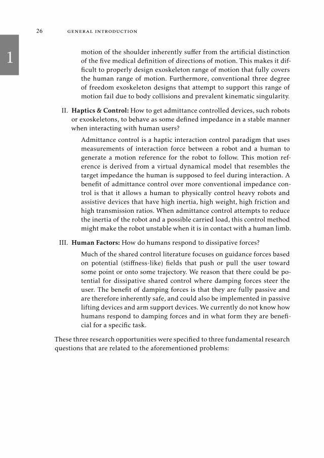
26 general introduction
motion of the shoulder inherently suffer from the artificial distinction
of the five medical definition of directions of motion. This makes it dif-
ficult to properly design exoskeleton range of motion that fully covers
the human range of motion. Furthermore, conventional three degree
of freedom exoskeleton designs that attempt to support this range of
motion fail due to body collisions and prevalent kinematic singularity.
II. Haptics & Control:How to get admittance controlled devices, such robots
or exoskeletons, to behave as some defined impedance in a stable manner
when interacting with human users?
Admittance control is a haptic interaction control paradigm that uses
measurements of interaction force between a robot and a human to
generate a motion reference for the robot to follow. This motion ref-
erence is derived from a virtual dynamical model that resembles the
target impedance the human is supposed to feel during interaction. A
benefit of admittance control over more conventional impedance con-
trol is that it allows a human to physically control heavy robots and
assistive devices that have high inertia, high weight, high friction and
high transmission ratios. When admittance control attempts to reduce
the inertia of the robot and a possible carried load, this control method
might make the robot unstable when it is in contact with a human limb.
III. Human Factors: How do humans respond to dissipative forces?
Much of the shared control literature focuses on guidance forces based
on potential (stiffness-like) fields that push or pull the user toward
some point or onto some trajectory. We reason that there could be po-
tential for dissipative shared control where damping forces steer the
user. The benefit of damping forces is that they are fully passive and
are therefore inherently safe, and could also be implemented in passive
lifting devices and arm support devices. We currently do not know how
humans respond to damping forces and in what form they are benefi-
cial for a specific task.
These three research opportunities were specified to three fundamental research
questions that are related to the aforementioned problems:

1
1.5 dissertation outline and scientific contributions 27
Research Questions
I. How to support the full range of motion of the human shoulder?
II. How to implement stable admittance control with inertia reduc-
tion?
III. How do humans respond to dissipative shared control forces?
These three main research questions separate this dissertation into three major
parts, as is explained in more detail in the following section.
1.5 dissertation outline and scientific contributions
The chapters in this dissertation, excluding the introduction and discussion,
were written as journal or peer-reviewed conference publications. This causes
some overlap between some chapters, but allows the reader to read most of
them individually or out of order. Many chapters do not focus on a solution
for exoskeletons specifically, because the work presented is more generally ap-
plicable.
Part I: Motion & Kinematics: Supporting the Human Shoulder. This part fo-
cuses on the range ofmotion of the human shoulder girdle and an accompanying
conceptual four degree of freedom kinematic exoskeleton design for a shoulder
joint.
Chapter 2 presents a novel visualization method to display and communi-
cate the rotational range of motion (ROM) of both the human shoulder gir-
dle and devices that possibly support such motions. The ROM of the hu-
man shoulder is commonly presented along five medical directions of mo-
tion. This neglects any coupling in ROM between these directions, which are
henceforth also neglected in exoskeleton and device design. Compared to
existing methods, our method is based on the fact that the rotation of the up-
per arm can be decomposed into three angles that are displayed on a discrete
grid in a two-dimensional Mollweide map projection. This avoids the need
to show several three-dimensional figures in two-dimensional print to show
and communicate the shoulder ROM. This makes it possible to evaluate hu-
man ROM, to evaluate visually how the ROM coupled between movement
directions, evaluate influence of pathologies and their recovery on shoulder
ROM, and make comparisons between the ROM between humans and de-

1
28 general introduction
vices. The method also allows to show quantitative device properties such as
joint conditioning (displaying kinematic singularity) and dynamical param-
eters, or human movement properties such as forces, movement times and
targeting variance.
Chapter 3 presents a differential inverse kinematics (IK) solution method of
a novel four degree of freedom (4R) exoskeleton design to assist the full range
of motion of the human shoulder. An additional, fourth, actuated degree of
freedom is used to achieve one degree of freedom of movement redundancy.
This redundancy is exploited to avoid kinematic singularity, and body and
limb collision. Redundancy resolution is performed through nullspace mo-
tions, without influencing the movement of the arm. Instead of gradient pro-
jection of some secondary objective, feedback along the one-dimensional self-
motion-manifold steers the exoskeleton towards more preferred configura-
tions. Compared with existing three degree of freedommethods this method
allows for a larger, singularity-free workspace of the exoskeleton joint. Com-
paredwith a recently published other 4R exoskeleton that used a non-differential
IKmethod, our method optimizes to find a kinematically more favorable con-
figuration on-line, even while the human arm is stationary.
Part II: Haptics & Control: Admittance Control. This part focuses on admit-
tance control. Admittance control is an interaction control method that relies
on force measurement from the user. The user’s force is effectively amplified by
calculating an exoskeleton reference motion through a virtual dynamical model.
The exoskeleton moves according to the model, and the apparent mechanical
impedance felt by the user approaches that of the virtual model. The stability of
such a control method during physical interaction with human users is not triv-
ial. Especially when the device is being held by a user this interaction method
can become unstable if it attempts to reduce the inertia of the device and carried
loads. The advantage of using admittance control over impedance control is that
it allows a human to physically control heavy robots and assistive devices that
have high inertia, high weight, high friction and high transmission ratios while
simulating damping and varying stiffness values in a stable way, required for
assistive tasks.
Chapter 4 presents an analysis of admittance control as an interaction con-
trol method, and provides a new set of guidelines on how to implement
admittance control to achieve apparent inertia reduction for the user. The
design guidelines are derived from a desire for device passivity; dynamical
behavior where the device can deliver no excessive amount of energy back

1
1.5 dissertation outline and scientific contributions 29
to the human operator. In this way, safety and stability can be guaranteed
during physical human-robot interaction.
Chapter 5 presents the cause of active behavior of naive admittance control
implementations. It shows why recently proposed methods to attempt time-
domain passivity control cannot be used to reduce the apparent device iner-
tia. Our work presents a different stabilization method: a passivity inspired
variable virtual damping controller for admittance control that stabilizes in-
teraction with stiffness-like environments. By keeping track of the stored
energy in the virtual model dynamics and the exchanged energy between
the device and the human operator, a variable damper is switched on or off
in the virtual model. Although passivity cannot be achieved, nearly passive
and stable behavior can be guaranteed.
Part III: Shared Control: Damping Forces around Reaching Targets. This part
focuses on a simple form of shared control: applying damping forces to a de-
vice and user during reaching movements. Such reaching movements represent
transportation movements performed by workers in real-world settings. Simple
sensors can gather limited environment information and the shared controller
applies these damping forces to assist the user in accurate placement and faster
movements towards task related targets.
Chapter 6 presents the evaluation of a novel simple haptic shared controller
based on damping forces. By assisting goal directed movements with damp-
ing around reaching targets, it is shown that humans increase their reaching
accuracy as well as decrease their movement times, when compared to free
conditions. The relation between increasing end-point accuracy and distance
and increasing movement time, known as Fitts’ Law, is shown to hold for
these dynamical conditions as well.
Chapter 7 presents an addendum to Chapter 6. Here, the evidence for how
human subjects are able to decrease reaching time while subjected to lon-
gitudinal haptic damping forces is discussed. We state the hypothesis that
damping forces mitigate the mechanical effects of activation dependent (or
multiplicative) motor noise. The attenuation of these effects of noise on end-
point accuracy allows for higher muscle forces and accelerations, while still
guaranteeing the requested accuracy. Nonlinear stochastic optimal control
models show agreement with measured data. This supports the hypothesis
that humans preform their reaching movements while optimizing for energy
efficiency and minimizing variance to an amount that the task requires.


Part I
MOTION & KINEMATICS :SUPPORTING THE HUMAN SHOULDER


2
2VI SUAL IZAT ION OF SHOULDER RANGE OF MOTION FOR
CL IN ICAL DIAGNOST ICS AND DEV ICE DEVELOPMENT
Arno H.A. Stienen and Arvid Q.L. Keemink
Burdens are for shoulders strong enough to carry them.
— Margaret Mitchell, Gone with the Wind, 1936
Abstract–Rotations of the humerus in the human shoulder girdle are usu-
ally described using five classical medical definitions: flexion/extension, ab-
duction/adduction, internal/external rotation, horizontal abduction/adduction,
and horizontal flexion/extension. The latter two are needed to overcome the
inability of the first three to define the full range of motion. The Interna-
tional Society for Biomechanics recommendations reduce these to three se-
quential rotations around perpendicular axes: rotation of the plane of eleva-
tion (horizontal rotation), elevation, and axial rotation. We expand on this
work by providing a new and intuitive visualization method to display these
rotations that superimposes the axial rotation on the map projection of the
reachable workspace of the elbow. We provide methods to interpret and cre-
ate the visualization using direct observations. The visualization allows the
immediate observation of the full rotational range of motion of the humerus
and the interaction effects between these physiologically coupled rotations.
Furthermore, it allows visualization of the effects of kinematic limitations of
external devices such as endpoint manipulators or exoskeletons. Therefore,
the new visualization method is useful for both clinical diagnostics and de-
vice development.
This chapter was published as: A.H.A. Stienen and A.Q.L. Keemink, “Visualization of shoul-der range of motion for clinical diagnostics and device development”, IEEE/RAS-EMBS Interna-tional Conference on Rehabilitation Robotics (ICORR), 2015. Both authors contributed equally tothis work.
33
2
34 visualization of shoulder range of motion
list of used symbols and abbreviations
Symbol Explanation
x, y, z vectors of principal axes
X, Y , Z positive directions along principal axis vectors
X, Y , Z negative directions along axis vectors
γa axial glenohumeral rotation angle
γe glenohumeral elevation angle
γh horizontal glenohumeral rotation angle
Abbrev. Explanation
GH glenohumeral
ISB International Society for Biomechanics
ROM range of motion
2.1 introduction
In this work we present a novel and intuitive visualization method for display-
ing the kinematics of the glenohumeral (GH) rotations of the human shoulder
girdle. The visualization method displays the rotations of the girdle via super-
position of the axial rotation on the map projection of the reachable workspace
of the elbow. An example of the visualization is given in Fig. 2.1.
The human shoulder girdle is a complex skeletal structure with a remarkably
large range of motion (ROM). Many havemeasured the GH rotations [22, 23, 24],
using a selection of the five classical movement directions: flexion/extension, ab-
duction/adduction, internal/external rotation, horizontal abduction/adduction,
and horizontal flexion/extension (see Fig. 2.2). These classical movements are
conceptually easy to understand, but the inclusion of the latter two is needed
to overcome the inability of the first three to define the full range of motion.
Furthermore, the rotations are defined around an immovable global joint coor-
dinate system that makes sequential rotations around multiple of the defined
axes prone to interpretation differences. To solve these problems, the Interna-
tional Society for Biomechanics (ISB) recommendations reduce these five classi-

2
2.1 introduction 35
-90
-60
-30
03
06
09
01
20
15
01
80
21
02
40
27
0
30
60
90
12
0
15
0
0
18
0
GHElevationRotation[]
GH
Ho
rizo
nta
lR
ota
tio
n[]
- 0 +
a
b
a
b
Figure
2.1:V
isualizationexam
ple
ofthemeasu
redrotational
rangeofmotionoftherighthumerusofasingle
subject.The
sphereoftheworksp
aceoftheelbow,asdefi
ned
bytheglenohumeral
(GH)horizo
ntalan
delevationrotationsalone,
isflattened
usingtheMollweidemap
projection.T
heprojectionisviewed
from
anexternal
observer
lookingat
the
subject.TheGH
axialrotationsareshownas
arcs
atdiscretegrid-points,witheach
arcrepresentingthereachab
lemovem
entoftheforearm
withan
(imag
inary)flexed
elbowat
90 ,as
seen
from
theobserver
when
lookingthrough
theresp
ectivegridpointat
theGH
rotationcenter.Theshad
edbackgroundarea
showsthereachab
lean
glesin
GH
horizo
ntalan
delevationrotation.R
ight:tw
oexam
plesofarm
orien
tations(a Oan
dbO)map
ped
tothecorresponding
locationan
dorien
tationthemap
projection.

2
36 visualization of shoulder range of motion
flexion
extension
(a)
abduction
adduction
(b)
external(lateral)
internal(medial)
(c)
h. flexion
h. extension
(d)
h. adduction
h. abduction
(e)
Figure 2.2: The five classical definitions of movement directions for three degrees of free-dom of the shoulder: a) flexion/extension, b) abduction/adduction, c) inter-nal/external rotation, d) horizontal flexion/extension, and e) horizontal ab-duction/adduction.
cal rotations to three sequential rotations around perpendicular axes [25]: GH
rotation of the plane of elevation, GH elevation (negative), and GH axial rota-
tion*. In this chapter we will use the ISB definitions but refer to them as GH
horizontal rotation, GH elevation rotation, and GH axial rotation for brevity
and clarity.
Independent of the joint coordinate system used, nearly all studies that re-
port on the GH ROM give the measurements for each axis as an independent
outcome measure. This ignores the interaction effects between these physiolog-
ically coupled rotations and leads to a reported ROM that is likely larger than
*As in [25], the methods presented here are valid for the right shoulder only. Whenever leftshoulders are measured, it is recommended to mirror the raw position data with respect to thesagittal plane. Finally, this chapter focuses on the GH rotations only and ignores any translations ofthe GH rotation center.
2
2.2 background 37
actually achievable. This might especially affect reporting in clinical diagnostics,
which require the ROM to be measured and represented properly.
External interaction with the shoulder girdle is possible with a wide variety
of devices, from endpoint manipulators and weight-support devices to exoskele-
tons and orthotics. Of these, exoskeletons are often used to directly augment the
three rotations of the GH joint [26, 27, 14, 15]. Again, common presentations
of human shoulder or exoskeleton shoulder ROM results are tables or graphs
that indicate by numerical intervals or plotted bars the ROM along the move-
ment directions [22, 28, 29, 30, 31, 32, 33, 34], under the assumption that these
movement ranges are decoupled. In [35, 26, 36, 27] a more graphical approach
is taken. They visualized the range of motion by creating a 3D point cloud
around the human body, indicating the reachable workspace of the human arm.
The third rotation, GH axial rotation, is not represented in these point clouds.
The globe system [37] recognizes that a sphere of elbow positions around the
humeral head is fully defined by GH horizontal and elevation rotations. It gives
the same angle definitions as the ISB recommendations to decompose arm ro-
tations onto this sphere. The axial rotation component is mainly neglected, or
drawn on a front or top view of the sphere. In publication, it presents only sin-
gle arm configurations using multiple top and side views, and gives therefore
no information about shoulder ROM. All these presentation methods have in
common that they are often hard to interpret due unintuitive representations or
by attempting to show 3D objects in 2D print.
We have therefore built upon the aforementioned work an developed a new
visualization method to show the complete shoulder ROM.With this method
we can inspect functional ROM of patients, compare the human shoulder ROM
to an exoskeleton shoulder ROM, or compare different exoskeleton shoulders.
Furthermore, we will use this visualization to show kinematic or dynamic prop-
erties of exoskeleton shoulder joints.
2.2 background
2.2.1 Kinematics of the Human Shoulder
To geometrically describe the human shoulder, we use axes and angles defini-
tions from the ISB [25]. As shown in Fig. 2.3, a global coordinate frame is at-
tached to the center of rotation in the glenohumeral (GH) rotation center of the
shoulder. The global x-axis points in the dorsoventral direction (forward), the

2
38 visualization of shoulder range of motion
z
y
γex
zγh
−γa
0
1 12
2
3
Figure 2.3: ISB Axes definitions, x pointing forward, y pointing upward and z pointingoutward. Intuitive ISB angle decomposition from left to right; Front view:GH elevation rotation first (from pose 0O to 1O, over angle γe). Top view: ro-tate horizontally (from pose 1O to 2O, over angle γh). View perpendicular tothe upper arm: finally, rotate axially (from pose 2O to 3O, over angle γa). Thisdecomposition is intuitively understood when performed by a person in a dif-ferent order than the geometrical ISB description, due to the singular natureof their proposed YXY rotation order
global y-axis points in the anteroposterior direction (upward) and the global
z-axis points into the mediolateral direction (outward to the right).
The human shoulder orientation is decomposed around these axes into YXY
intrinsic Euler angle rotations. These rotations are stated in the order of most
to least dominant rotation, i.e. a dominant rotation also rotates a less dominant
axis. Classically this YXY decomposition would be (dominant) Y : horizontal ab-
duction/adduction, X: abduction/ adduction or flexion/extension (dependent
on the configuration), and (least dominant) Y : internal/external rotation.
The shoulder rotates a person’s upper arm, which makes the tip of the elbow
cover part of the surface of a sphere (i.e. the ‘elbow-tip sphere’). This sphere
can be decomposed into spherical coordinates: the GH horizontal rotation γhand GH elevation rotation γe (the first two most dominant YX rotations). The
third and least dominant upper arm rotation, GH axial rotation, is described
directly by γa, relative to the horizontal plane. Positive GH elevation rotation
is defined as a clockwise rotation in the rotated elevation plane around the ro-
tated x-axis. The GH horizontal rotation is defined as counter-clockwise around
the global y-axis, with 0 GH horizontal rotation making the GH elevation rota-
tion pure shoulder ab-/adduction, and 90 GH horizontal rotation making GH
elevation rotation pure shoulder flexion/extension. The GH axial rotation is de-

2
2.2 background 39
fined as being positive in clockwise direction (i.e. positive for internal/lateral
rotation) around the upper arm vector (not common for right handed coordi-
nate systems).
This decomposition is intuitively understood when performed by a person in
a different order than the geometrical description, due to the singular nature
of the YXY rotation order (i.e. the unresolvable ambiguity between horizontal
and axial rotation in some orientations). The intuitive decomposition is shown
in Fig. 2.3 and described as follows:
1. First, a person elevates the arm from the zero-configuration (rotation from
orientation 0O to 1O over angle γe)
2. Secondly, the person performs horizontal rotation (rotation from orienta-
tion 1O to 2O, over angle γh).
3. Finally, the person rotates axially (rotation from orientation 2O to 3O, over
angle γa.
Our initial- or zero-configuration is defined as the one with the upper arm point-
ing vertically down (orientation 0O in Fig. 2.3). In the zero-configuration the el-
bow is touching a person’s side. For ease of reasoning, and to avoid ambiguity,
we always assume 90 elbow flexion.
2.2.2 Kinematics of the Exoskeleton Shoulder
For any exoskeleton shoulder we will use the same global axes as for the human
shoulder (Sec. 2.2.1). Generically, a shoulder exoskeleton is regarded as a series
of three sequential rotations. Although parallel exoskeleton shoulder actuation
does exist [30], in this work we will compare several exoskeleton shoulder de-
sign configurations conceptually in Sec. 2.4.
The order of rotations in the human’s zero configuration we will call the ex-
oskeleton’s rotation order. If the rotation order is for instance XYZ , this implies
that the first (most dominant) rotation axis is the global x-axis, the second rota-
tion axis is the global y-axis and the third (least dominant) rotation axis is the
global z-axis. Note that these axes only coincide with the global axes in the hu-
man’s zero orientation, and the second and third axes will be rotated away from
the principal axes by moving the human arm.
Common rotation orders are the orthogonal designs (a bar denoting negative
direction): YZY , XYZ , XZY and YXZ . Also, several designs place the first rota-
tion axis in none of the principal directions [38, 29, 39] and do not necessarily

2
40 visualization of shoulder range of motion
Table 2.1: Joint zero-configurations of exoskeleton shoulder designs. *Rotated Z , **FirstAxis < 45 rotated away from principal. A bar implies negative direction.
Order Name[14, 15]
YZY ArmeoPower, ARMIN (chARMin, I-IV), Dampace, ExoRob, FRE-FLEX, IntelliArm, Limpact, (pneu-)WREX∗, SUEFUL-7
XYZ ABLE, BONES
XZY L-Exos, CADEN-7∗∗, RehabExos∗∗, Salford ARE(∗)
YXZ MEDARM∗∗, MGA∗∗, MULOS∗
have the same kinematic properties as the four major orders. A list of several
common designs is shown in Table 2.1. Useful references to these designs can
be found in [14] and [15].
2.3 method
2.3.1 Shoulder ROM Projection
We choose the Mollweide (or homolographic) projection [40] to expand a spheri-
cal surface onto a 2D plane. TheMollweide projection is preferred to an equirect-
angular projection (in which points of GH elevation andGH horizontal rotations
form a rectangular grid), due to the equirectangular projection’s ambiguity at the
poles and the Mollweide projection’s aesthetic properties.
We place the 90 GH elevation rotation and 90 GH horizontal rotation in
the center of the map, as is shown by a gray human figurine in the background
of the figure holding its arm in γh = 90, γe = 90, γa = 0 orientation. Thischanges the map range from 0 to 180 in GH elevation rotation and −90 to270 in GH horizontal rotation, compared to conventional world maps in longi-
tude and latitude. The +270 meridian is equivalent to the −90 meridian, and
is therefore never used and shown as a dashed line. Equations to calculate the
projection can be found in Appendix A.
In addition, we can also show the complete GH horizontal and elevation bounds
by using a half-transparent shaded area, as is done in Fig. 2.1 and Fig. 2.5. This
area is most of the time left out if it is irrelevant, and to limit the amount of
information presented to the reader.
2
2.3 method 41
-90 -60 -30 0 30 60 90 120 150 180 210 240 270
30
60
90
120
150
0
180
GH
Ele
vat
ion
Rota
tion[]
GH Horizontal Rotation []
-0+
Human
Human ADL
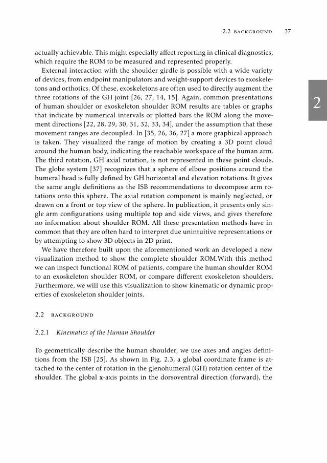
Figure 2.4:Measured ROM of the subject compared to specified ROM ADL-movementsas measured in [24].
2.3.2 Showing Axial Rotations
The GH axial rotation ROM of the shoulder is shown on the Mollweide-grid on
discrete locations. Discrete intervals are usable since the axial ROM varies rather
smoothly over the complete sphere of GH horizontal and elevation rotation. The
axial ROM is shown as an arc. Counter-clockwise rotation is negative axial rota-
tion (i.e. external rotation), clockwise is positive axial rotation (i.e. internal rota-
tion). Notice the small 0, − and + sign at the 90 elevation pose of the figurine
in the background in Fig. 2.1. In this work we space these arcs on intervals 30
apart in horizontal and elevation rotation, although greater and smaller inter-
vals are possible. If only a single axial orientation is shown (instead of a range),
a thicker single line (like a clock hand) is shown, as is done in Fig. 2.1 for two
example arm orientations.
2.3.3 Measurement Method
Tomeasure the ROM of the shoulder we propose the following method to be per-
formed for reachable chosen grid-points (a visual representation of the method
is given in Fig. 2.3). This might not be an optimal way to determine the shoul-
der ROM, but we would like to emphasize that the visualization and not the
measurement method is of main interest in this work. The method used to gen-
erate results in Sec. 2.4 is as follows:
2
42 visualization of shoulder range of motion
-90 -60 -30 0 30 60 90 120 150 180 210 240 270
30
60
90
120
150
0
180
GH
Ele
vat
ion
Rota
tion[]
GH Horizontal Rotation []
-0+
Human
Dampace
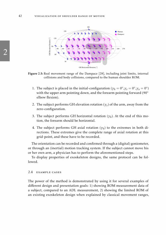
Figure 2.5: Real movement range of the Dampace [28], including joint limits, internalcollisions and body collisions, compared to the human shoulder ROM.
1. The subject is placed in the initial-configuration (γh = 0,γe = 0,γa = 0)with the upper arm pointing down, and the forearm pointing forward (90
elbow flexion).
2. The subject performs GH elevation rotation (γe) of the arm, away from the
zero-configuration.
3. The subject performs GH horizontal rotation (γh). At the end of this mo-
tion, the forearm should be horizontal.
4. The subject performs GH axial rotation (γh) to the extremes in both di-
rections. These extremes give the complete range of axial rotation at this
grid-point, and these have to be recorded.
The orientation can be recorded and confirmed through a (digital) goniometer,
or through an (inertial) motion tracking system. If the subject cannot move his
or her own arm, a physician has to perform the aforementioned steps.
To display properties of exoskeleton designs, the same protocol can be fol-
lowed.
2.4 example cases
The power of the method is demonstrated by using it for several examples of
different design and presentation goals: 1) showing ROM measurement data of
a subject, compared to an ADL measurement, 2) showing the limited ROM of
an existing exoskeleton design when explained by classical movement ranges,

2
2.4 example cases 43
-90 -60 -30 0 30 60 90 120 150 180 210 240 270
30
60
90
120
150
0
180
GH
Ele
vat
ion
Rota
tion[]
GH Horizontal Rotation []
-0+
(a) YZY
-90 -60 -30 0 30 60 90 120 150 180 210 240 270
30
60
90
120
150
0
180
GH
Ele
vat
ion
Rota
tion[]
GH Horizontal Rotation []
-0+
(b) XYZ
-90 -60 -30 0 30 60 90 120 150 180 210 240 270
30
60
90
120
150
0
180
GH
Ele
vat
ion
Rota
tion[]
GH Horizontal Rotation []
-0+
0 0.2 0.4 0.6 0.8 1
Exoskeleton Conditioning
(c) XZY
Figure 2.6: Illustration of conditioning of three common rotation orders: a) YZY b) XYZc) XZY . Joint conditioning is shown as a red-to-green gradient (red = gimballock, green = perfect conditioning).

2
44 visualization of shoulder range of motion
-90 -60 -30 0 30 60 90 120 150 180 210 240 270
30
60
90
120
150
0
180
GH
Ele
vat
ion
Rota
tion[]
GH Horizontal Rotation []
-0+
Human
Exosk
(a)
-90 -60 -30 0 30 60 90 120 150 180 210 240 270
30
60
90
120
150
0
180
GH
Ele
vat
ion
Rota
tion[]
GH Horizontal Rotation []
-0+
Human
Exosk.
(b)
Figure 2.7: Implications of choosing mechanical joint limits in exoskeletons. a) All rota-tions of the exoskeleton limited to the minimum range b) All rotations of theexoskeleton limited to the maximum range. Both figures are only valid forYZY or YXY .
3) showing kinematic exoskeleton design properties in terms of kinematic con-
ditioning, 4) showing the complexity of the design problem of choosing mechan-
ical joint limits for exoskeleton design.
The method was used to determine the human ROM (a healthy male subject,
19 y.o.), shown in Fig. 2.4. The subject was measured using a goniometer. Cou-
pling is observed between the GH horizontal and GH elevation rotation and the
range of GH axial rotation. The ROM is compared to the one measured in [24]
for ADL movements to show that moving along the classical directions shows a
different determined ROM without coupling effects. It cannot be ruled out that
the different size of ROM is due to the subject(s) or the method.

2
2.5 discussion 45
We show in Fig. 2.5 the measured ROM of the passive Dampace Exoskele-
ton [28], including the complete GH horizontal and elevation region in the
shaded area. We compare the measured range with the human one, to show
how well the exoskeleton supports the human ROM.
Next, we show the kinematic conditioning of three main exoskeleton shoulder
types YZY , XYZ and XZY in Fig. 2.6. The exoskeleton conditioning is calcu-
lated by taking the absolute determinant of only the square rotation Jacobian of
the system. The conditioning ranges therefore in value from 0 to 1. The figures
directly show the benefits of several rotation orders for a specified task ROM.
It also shows that some rotation orders, such as XZY are better avoided. There-
fore in [29] they actually placed the first axis under a 45 angle, moving the
singularity towards higher GH horizontal rotation angle.
Finally, we use the measurement data to show extreme choices of mechani-
cally limiting rotations for YZY and YXY rotation orders (or for inverted ver-
sions of the rotation axes). If the minimal rotation ranges are picked, as in
Fig. 2.7a, the design is very safe, but very conservative and unusable. If the max-
imal rotation ranges are picked, as in Fig. 2.7b, the human achieves full range of
motion, but the exoskeleton cannot be inherently mechanically safe and needs
angle limitations in software.
2.5 discussion
The visualization method can be used to display a large variety of useful infor-
mation about standard human shoulder ROM, pathological ROM, ADL ROM,
assistive device ROM and mechanical, kinematic or dynamic device properties.
Compared to presentation of classical movement ranges of the human shoul-
der in tables, this method does take more publication space, but gives a more
complete picture. The addition of our method to the globe system[37] is the pos-
sibility to show complete ROM directly, including axial rotation, without using
different camera viewpoints. Compared to plotting 3D points or a surface in a
2D image, our method is clear and less ambiguous, also directly including GH
axial rotations.
Using our method to display device ROM is useful if its ROM is compared
to the human ROM and show its dynamic or kinematic properties over the hu-
man workspace. For a separate robotic device the joint limits could already be
sufficient to determine their own complete ROM.
2
46 visualization of shoulder range of motion
The given examples demonstrate that for a select set of challenges, the ex-
tended effort needed to acquire the full set of measurements needed for the
visualization are worth the effort in collection.
A minor drawback, due to the ISB decomposition of rotation into three Euler
angles, is the representation singularity in the arm’s zero-configuration. A shoul-
der flexion to hyper-extension motion with the forearm forward would imply an
instantaneous 180 jump in GH horizontal (from +90 to −90) and GH axial
rotation (from +90 to −90). This jump in angles is counter-intuitive.
Future work will include simplifying the required data collection, using in-
ertial measurement systems. Measuring more subjects will help introducing a
statistical certainty measure of the achieved ROM, which can be included in the
visualization. Finally, this method will be evaluated with clinicians, industrial
partners to show its usefulness in displaying progression of shoulder rehabilita-
tion and the benefit of assistive and rehabilitation devices.

3
3DIFFERENT IAL INVERSE K INEMAT ICS OF A REDUNDANT
4R EXOSKELETON SHOULDER JO INT
Arvid Q.L. Keemink, Gijs van Oort, Martijn Wessels and Arno H.A. Stienen
The Singularity is Near.
— Raymond Kurzweil, 2006
Abstract–Most active upper-extremity rehabilitation exoskeleton designs in-
corporate a 3R rotational shoulder joint with orthogonal axes. This kind of
joint has poor conditioning close to singular configurations when all joint
axes become coplanar, which reduces its effective range of motion. We inves-
tigate an alternative approach of using a redundant non-orthogonal 4R rota-
tional shoulder joint. By inspecting the behavior of the possible nullspace
motions, a new method is devised to resolve the redundancy in the differ-
ential inverse kinematics (IK) problem. A 1D nullspace global attraction
method is used, instead of naive nullspace projection, to guarantee proper
convergence. The design of the exoskeleton and the proposed IK method en-
sure good conditioning, avoid collisionswith the human head, arm and trunk,
can reach the entire human workspace, and outperforms conventional 3R or-
thogonal exoskeleton designs in terms of lower joint velocities and by avoid-
ing body collisions.
list of used symbols and abbreviations
Symbol Explanation
∅ the empty set
Ans(Γ,q) subset of Cns reachable from current joint configuration
Cns(Γ) self-motion-manifold of exoskeleton or arm configuration
Dns(Γ,q) subset of Cns disjointed from current joint configuration
eQ scalar feedback error along QnsThis chapter is under review in the IEEE/RAS-EMBS Transactions on Neural Systems & Reha-
bilitation Engineering (TNSRE).
47

3
48 differential i.k. of a redundant 4r exoskeleton shoulder
f (q) scalar potential parameterized by joint angles q
F (q) generic form of a forward kinematic function
g super-/subscript: relating to the global reference frame
li subscript: relating to exoskeleton links
J(q) geometrical Jacobian
k discrete-time time instant
K feedback gain
ns subscript: related to the nullspace motions
N (·) the nullspace of the matrix argument
P(q) nullspace projector matrix
q vector of joint angles
q+ a valid configuration in the next self-motion-manifold
q∗ joint-space attractor
qm the minimal point, closest to the attractor
qmn differential inverse kinematics minimum-norm solution
qns,0 initial configuration of the self-motion-manifold
Qns(Γ,q) subset of Cns connected to current joint configuration
r link radius
R three-dimensional rotation matrix
R the set of all real numbers
SO(3) group of all 3D rotations about the origin
t time
T discrete sample time
u unit-vector
uN basis of the nullspace of the Jacobian
ua subscript: relating to the human’s upper arm
U, V left and right eigenvector matrices as result from SVD
w any dummy vector in R4
Wh human shoulder workspace
x, y, z principal axes vectors
x, y, z subscript: directions
X, Y , Z positive directions along principal axis vectors
Z set of all the integer numbers

3
3.1 introduction 49
α swept angle of a collision cone
β scalar used to make tanh (βx) approach sgn(x)
γa axial glenohumeral rotation angle
γe glenohumeral elevation angle
γh horizontal glenohumeral rotation angle
Γ vector of shoulder angles
δ(ξ) scalar distance along Cns∆x spatial numerical integration step
η conditioning threshold
θ relative rotation of the first axis of rotation
Θ vector of relative rotations of the first axis of rotation
λ eigenvalue
ρ nullspace vector scalar
σ singular value
Σ matrix of singular values as result from SVD
φ exoskeleton arc
Φ vector of exoskeleton arcs
ξ joint-space integration variable
ω vector of axis of rotation of the exoskeleton joints
Ω rotational velocity vector of the shoulder
Abbrev. Explanation
nR n degrees of freedom of rotation
CoR center of rotation
DOF degree of freedom
IK inverse kinematics
SVD singular value decomposition
3.1 introduction
Upper-Extremity exoskeletons are commonly used for rehabilitation purposes,
tele-operation and task training [39, 41, 14, 15]. One major issue with these

3
50 differential i.k. of a redundant 4r exoskeleton shoulder
ω1
ω2
ω3
ω4
CoR
Figure 3.1: Schematic overview of the proposed 4R shoulder joint, showing a person us-ing the exoskeleton joint to move the upper-arm. The joint is comprised ofthree concentric arcs with decreasing radii. The dashed arrows indicate thefour rotation axes of the joint that intersect in the Center of Rotation (CoR).Note that the fourth joint axis is inside the human arm. Translations of theshoulder complex will be taken care of by an external translation mechanism[43] attached to the first motor (not shown).
conventional exoskeletons is that they cannot match the full human shoulder
workspace due to conditioning and collision problems.
The shoulder of upper-extremity rehabilitation exoskeletons usually comprises
three sequential rotational (3R) degrees of freedom (DOFs) [42, 39, 43]. Such a
system’s kinematics are fully described by three implicit Euler angles. Any sys-
tem with sequential rotations has singular configurations, also known as gimbal
lock, when rotation axes become collinear or coplanar. During gimbal lock in a
shoulder exoskeleton joint the user loses one rotational direction to move in [44].
Near the singular configuration an inverse kinematics algorithm has to handle
the poor conditioning, which results in high motor velocities and high experi-
enced inertia.
We propose to add an extra rotational DOF to the exoskeleton joint, and to
make all four rotation axes non-orthogonal in order to 1) avoid singular configu-
rations, 2) make it easier to avoid collisions with the human body and 3) achieve
a range of motion larger than the one of the human shoulder. An example de-
sign is shown in Fig. 3.1. The 4R shoulder joint is to be used in 3R admittance
control mode with bounded velocities and accelerations, similar to [39, 45, 46].
Therefore, we need an inverse kinematics (IK) algorithm to pick a good set of
four joint angles, or their velocities, that imposes the right orientation on the
human shoulder without precomputed trajectories.
3
3.1 introduction 51
A 4R shoulder joint for exoskeletons has been implemented twice recently.
In [47, 48, 49], a one-to-one configuration mapping with unexplained interpo-
lation on 89 upper-arm configurations is used. A non-orthogonal exoskeleton
configuration was found through a genetic algorithm. Although their method
appears to work, it does not give insight into the problem, and has no a-priori
guarantee or explanation if it will always work for any design. In [50], the focus
is on a passive orthogonal 4R exoskeleton for macaques. Their analysis focuses
on the theoretical feasibility of the 4R principle, to determine if avoiding joint
limits and poor conditioning is possible, and do not focus on any IK method.
They incorporate body collisions implicitly in the joint limits. They conclude
for their fully orthogonal design that it should be possible to always stay away
from gimbal lock and joint limit collisions.
The goal of this work is to detail the differential IK algorithm for this redun-
dant 4R exoskeleton shoulder joint. We focus solely on the rotation of the hu-
man shoulder, with translations of the joint [51, 52, 53, 39, 43] taken care of by
a translation mechanism [43]. Furthermore, the fourth rotation axis is initially
chosen to be parallel to the long axis of the upper arm, such that the problem
reduces in complexity to a 3R-to-2R mapping instead of a 4R-to-3R mapping.
3.1.1 Background
Avoiding gimbal lock for a 4R gimbal system was achieved by NASA for flight-
simulators [54, 55, 56]. A method was developed to steer the fourth, least domi-
nant, DOF to attempt to improve the gimbal conditioning. Their method works
in a collision-free setting, valid for flight-simulators, but will not work when
the human body restricts the solution space. Other 4R systems have been pro-
posed to rotate cameras [57]. They take advantage of nullspace motions and
DOF weighting in the Jacobian pseudo-inverse (see Sec. 3.2.5). This method too
is limited to collision-free settings. A general robotics redundancy resolution is
proposed by Siciliano et al. [58], by applying gradient-nullspace-projection (see
Sec. 3.4) of a (cost) minimization objective in jointspace. This commonly results
in achieving only local optima. The structure of the nullspace and constraints is
not analysed, making the resulting behavior sub-optimal and lacking any guar-
antees about conforming to constraints.
We expand on this previous work and propose a more generic method of anal-
ysis and solution to the problem for non-orthogonal 4R shoulders that explicitly
takes into account collision with the body and the human arm. We overcome

3
52 differential i.k. of a redundant 4r exoskeleton shoulder
some drawbacks of naive gradient projection, while ensuring quasi-static conver-
gence to a well-defined nullspace-configuration ‘minimum’. Although we will
discuss one specific design in this work, the analysis and IK method is applica-
ble to other 4R designs.
3.2 kinematics
We use ‘shoulder’ to refer to the human 3R shoulder joint and ‘exoskeleton’ to re-
fer to the new 4R exoskeleton joint. In the subsequent text, vectors and matrices
are denoted in boldface, and unit vectors are denoted by u. The only exceptions
are coordinate-frame axes which are given by x, y or z. A 3-by-3 rotation matrix
around a principal axis is specified by R ∈ SO(3), with subscript x, y or z.
3.2.1 Axes Definitions
For the shoulder and exoskeleton we use definitions of axes and angles from
the ISB [25], as shown in Fig. 3.2a and Fig. 3.2b. An inertial global frame is
attached to the glenoid in its Center of Rotation (CoR) of the shoulder. Any
vector expressed in this global frame will have left superscript g . For the right
arm, the global x-axis points in the dorsoventral direction (forward), the global
y-axis points in the anteroposterior direction (upward) and the global z-axis
points into the mediolateral direction (outward to the right).
3.2.2 Kinematics of the Shoulder
The human shoulder orientation can be decomposed around these three axes
into YXY intrinsic Euler angle rotations (stated in the order of most-middle-
least dominant, i.e. a more dominant rotation also rotates less dominant axes)
relative to the global frame. The angle decomposition is shown in Fig. 3.2c. The
zero-orientation is defined where the upper arm is pointing vertically down,
with the elbow touching a person’s side (see Fig. 3.2c arm pose 0O). Geometri-
cally the zero-orientation would give the upper-arm a unit vector in negative
global y, i.e. guua = −guy . The forearm would then point from the elbow for-
ward, parallel to gux.
The human elbow can reach a subset of points on the surface of a sphere, de-
fined by horizontal rotation γh and elevation rotation γe. The third axial upper-
arm rotation, internal and external rotation, is described directly by γa. These

3
3.2 kinematics 53
zgxg
yg
Ω
(a)
zgxg
yg
zuaxua
yua
(b)
zg
yg
γe
xg
zgγh
−γa
0
1 12
2
3
(c)
Figure 3.2: a) ISB axes definition of the global frame (xg , yg , zg ), showing also the rigidbody instantaneous rotational velocity vector of the shoulder Ω that willbring the upper arm to the configuration in b). b) Showing the rotated up-per arm (ua) frame (red) at the end of the rotation. c) Interpretation of theISB angle definitions (γh,γe ,γa) for decomposing the arm configuration in b).It is more insightful to elevate first (from pose 0O to 1O, over angle γe), thenrotate horizontally (from pose 1O to 2O, over angle γh) and then rotate axially(from pose 2O to 3O, over angle γa), as shown from left to right in the figure.In the actual ISB definitions, the arm orientation has to be decomposed (mostto least dominant rotation) into plane-of-elevation rotation (around yg , withangle γh), elevation rotation (around a rotated local X, with angle γe) and ax-ial rotation (around double rotated local Y , with angle γa). The mathematicaldescription is given in Sec. 3.2.2.

3
54 differential i.k. of a redundant 4r exoskeleton shoulder
angles are combined in Γ = [γh, γe, γa]T . Positive elevation is defined as a clock-
wise rotation around rotated X. The forward kinematics of the shoulder coordi-
nate frame are hence described by a chain of three rotation matrices
gRua(Γ) = Ry(γh)Rx(−γe)Ry(−γa). (3.1)
3.2.3 Exoskeleton Geometry
The exoskeleton comprises four revolute joints (the exoskeleton axes). The ori-
entation of the first rotation axis is rotated from gy over two sequential YX-
rotations Θ = [θ1, θ2]T , as shown in Fig. 3.3a. The four exoskeleton axes are
separated by three arcs Φ = [φ1, φ2, φ3]T , as shown in Fig. 3.3b. These arcs
are commonly 90 in 3R designs, but we choose a different design. The ro-
tational motor degrees of freedom are described by four rotation angles q =
[q1, q2, q3, q4]T . The zero-configuration of the exoskeleton is as it is spread out
in the singular plane (the YZ plane rotated over angles Θ) in Fig. 3.3b.
We found that for any 4R shoulder exoskeleton the joint axes do not have
to be perpendicular to be able to reach the complete range of all possible 3D
rotations in SO(3). To be able to generate all elements in SO(3) at least once,
the necessary and sufficient condition (Φ in radians) is
∥∥∥∥Φ −
π
2
∥∥∥∥1=
3∑
i=1
∣∣∣∣φi −
π
2
∣∣∣∣ ≤
π
2. (3.2)
Eq. (3.2) puts limits on valid combinations of arcs Φ.
For the conceptual design in Fig. 3.1 the design parameters are given in Ta-
ble 3.1. These design parameters were derived from analysing the exoskeleton
with the method outlined in this chapter to find a proper combination of de-
sign parameters. The sizes correspond to a developed 1:2 scale model of a 4R
exoskeleton, and they do not necessarily constitute proper mechanical design
optimized for stiffness and size. From Table 3.1 it can be seen that ‖Φ−π/2‖1 =5π/12, conforming to (3.2).

3
3.2 kinematics 55
Table 3.1: Design Parameters of the System
Symbol Value Explanation
θ1 [deg] -35 First axis angle Y
θ2 [deg] +90 Second axis angle X
φ1 [deg] 45 First link arc
φ2 [deg] 60 Second link arc
φ3 [deg] 90 Third link arc
η [-] 0.25 Conditioning threshold
r1 [m] 0.288 First link radius
r2 [m] 0.222 Second link radius
r3 [m] 0.156 Third link radius
rm [m] 0.037 Motor radius
ra [m] 0.06 Arm radius
ρ [rad/s] 1 NS integration velocity
∆T [s] 0.001 Discrete sample time
∆x [rad] 0.0001 Spatial integration step
3.2.4 Forward Kinematics of the Exoskeleton
The exoskeleton configuration (ua with respect to g) is a chain product of
gRua(q,Θ,Φ) = gR1(Θ)1R4(q,Φ)4Rua(q4), (3.3)
with gR1(Θ) the initial rotation over angles Θ, 1R4(q,Φ) the rotations over an-
gles q, separated by arcs Φ (see Fig. 3.3b.) and 4Rua(q4) the final axial rotation
of the upper arm. This gives the forward kinematics of the 4R exoskeleton joint.
Note that only q is controlled and Θ and Φ are design parameters.
The mechanical coupling of the shoulder and exoskeleton results in
gRua(Γ) =gRua(q,Θ,Φ), (3.4)
which forms the basis of the inverse kinematics problem.

3
56 differential i.k. of a redundant 4r exoskeleton shoulder
zgxg
yg
−θ1
θ2ω1
(a)
φ1
ω1
ω2
φ2
ω3
φ3
ω4
CoR
y1
z1
r1
(b)
Figure 3.3: a) Definition of Θ angles for rotating the first rotation axis ω1 relative toglobal gy. Only the first motor is shown for clarity. b) Definition of arcs (link‘lengths’) between two consecutive rotation axes given by φ1, φ2 and φ3. Theexoskeleton is placed in a singular YZ plane in the 1-frame. By definition,each rotation axis rotates around its local Y and is separated by an arc φj ,rotated around local X. The distance of the first motor w.r.t. the CoR is givenby r1. The human body is not shown for clarity.
3.2.5 Inverse Kinematics of the Exoskeleton
Solving the inverse kinematics (IK) problem means finding q or its time deriva-
tive from the known Θ, Φ and shoulder angles Γ, shoulder rotational velocity
Ω, and acceleration Ω (see Fig. 3.2a and Fig. 3.2b).
Solving the IK in (3.4) analytically is in general impossible and requires itera-
tive approaches or numerical integration. Another problem is that the exoskele-
ton is composed of 4-DOF, while the shoulder is uniquely described by 3-DOF
(when not in a representation singularity). Hence, there is no unique inverse
mapping.
First order differential forward kinematics are given by
gΩ =
(g Rua
gRTua
)∨= J(q)q, (3.5)

3
3.3 preliminaries 57
with (·)∨ the inverse skew-operator. Geometrically, Jacobian J(q) is comprised
of the four joint axes, expressed in the global frame:
J(q) =[gω1,gω2,
gω3,gω4] (3.6)
=[gR1(Θ)1uy ,gR2(Θ,φ1,q1)
2uy ,
gR3(Θ,φ1,φ2,q1,q2)3uy ,
gR4(Θ,Φ,q1,q2,q3)4uy ].
The Jacobian is not square and not directly invertible. A candidate inverse is the
one that minimizes the squared Euclidian-norm (L2) of the joint velocities. This
gives the minimum norm solution qmn:
qmn = JT (q)(
J(q)JT (q))−1 g
Ω (3.7)
= J†(q) gΩ.
The J†(q) is a right pseudo-inverse of J(q).This minimum norm solution gives joint velocities that might still make the
exoskeleton singular or collide with the human body, and is therefore not suffi-
cient to operate the exoskeleton.
A more general solution to the differential inverse kinematics is of the form
qik = qmn + qns, (3.8)
in which qns is a nullspace joint velocity [58] that is used to steer the exoskeleton
away from poor conditioning and body collisions, as will be explained in detail
in Sec. 3.3.2.
3.3 preliminaries
In this section we investigate the constraints and assumptions for our method.
An in depth analysis of the ‘nullspace motions’ is presented in Sec. 3.3.2-4.
3.3.1 Jointspace Constraints
During operation of the exoskeleton several events are not allowed to happen,
which are expressed as jointspace constraints. These constraints will be dis-
cussed in order of decreasing importance. Methods to calculate the constraints
can be found in the supplementary material.
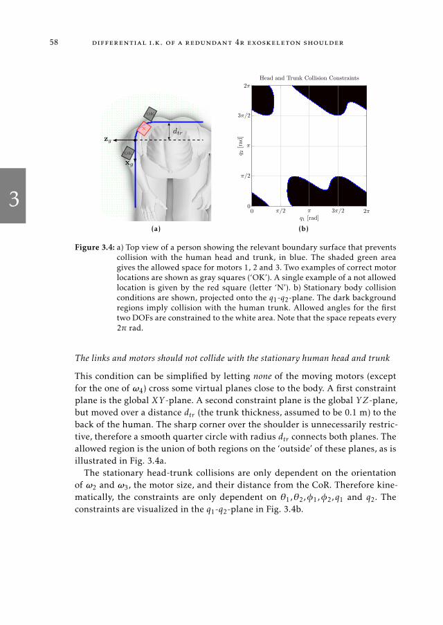
3
58 differential i.k. of a redundant 4r exoskeleton shoulder
dtrzg
xg
OK
OK
N
(a)
0
π/2
π
3π/2
2π
0 π/2 π 3π/2 2πq1 [rad]
q 2[rad
]
Head and Trunk Collision Constraints
(b)
Figure 3.4: a) Top view of a person showing the relevant boundary surface that preventscollision with the human head and trunk, in blue. The shaded green areagives the allowed space for motors 1, 2 and 3. Two examples of correct motorlocations are shown as gray squares (‘OK’). A single example of a not allowedlocation is given by the red square (letter ‘N’). b) Stationary body collisionconditions are shown, projected onto the q1-q2-plane. The dark backgroundregions imply collision with the human trunk. Allowed angles for the firsttwo DOFs are constrained to the white area. Note that the space repeats every2π rad.
The links and motors should not collide with the stationary human head and trunk
This condition can be simplified by letting none of the moving motors (except
for the one of ω4) cross some virtual planes close to the body. A first constraint
plane is the global XY -plane. A second constraint plane is the global YZ-plane,
but moved over a distance dtr (the trunk thickness, assumed to be 0.1 m) to the
back of the human. The sharp corner over the shoulder is unnecessarily restric-
tive, therefore a smooth quarter circle with radius dtr connects both planes. The
allowed region is the union of both regions on the ‘outside’ of these planes, as is
illustrated in Fig. 3.4a.
The stationary head-trunk collisions are only dependent on the orientation
of ω2 and ω3, the motor size, and their distance from the CoR. Therefore kine-
matically, the constraints are only dependent on θ1,θ2,φ1,φ2,q1 and q2. The
constraints are visualized in the q1-q2-plane in Fig. 3.4b.
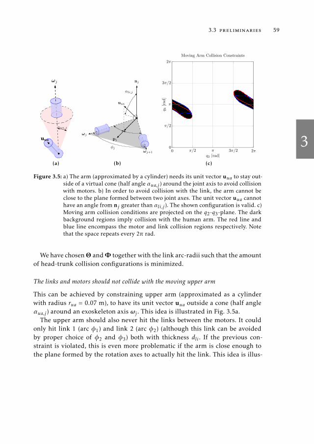
3
3.3 preliminaries 59
uuauua
ωj
αua,j
(a)
nj
φj
uua
pj
ωj
ωj+1
αli,j
(b)
0
π/2
π
3π/2
2π
0 π/2 π 3π/2 2πq2 [rad]
q 3[rad
]
Moving Arm Collision Constraints
(c)
Figure 3.5: a) The arm (approximated by a cylinder) needs its unit vector uua to stay out-side of a virtual cone (half angle αua,j ) around the joint axis to avoid collisionwith motors. b) In order to avoid collision with the link, the arm cannot beclose to the plane formed between two joint axes. The unit vector uua cannothave an angle from nj greater than αli,j ). The shown configuration is valid. c)Moving arm collision conditions are projected on the q2-q3-plane. The darkbackground regions imply collision with the human arm. The red line andblue line encompass the motor and link collision regions respectively. Notethat the space repeats every 2π rad.
Wehave chosenΘ andΦ together with the link arc-radii such that the amount
of head-trunk collision configurations is minimized.
The links and motors should not collide with the moving upper arm
This can be achieved by constraining upper arm (approximated as a cylinder
with radius rua = 0.07 m), to have its unit vector uua outside a cone (half angle
αua,j ) around an exoskeleton axis ωj . This idea is illustrated in Fig. 3.5a.
The upper arm should also never hit the links between the motors. It could
only hit link 1 (arc φ1) and link 2 (arc φ2) (although this link can be avoided
by proper choice of φ2 and φ3) both with thickness dli . If the previous con-
straint is violated, this is even more problematic if the arm is close enough to
the plane formed by the rotation axes to actually hit the link. This idea is illus-

3
60 differential i.k. of a redundant 4r exoskeleton shoulder
trated in Fig. 3.5b. The constraints are visualized in the q2-q3-plane in Fig. 3.5c.
Our choice of values for Φ ensures we can fully avoid arm collision with link 2.
The motors should not collide with other motors
By designing the link arcs and radii properly, this problem can be fully avoided.
Hence this is not further discussed.
The exoskeleton should not approach singularity
The exoskeleton is only fully singular (rank 2) if all joint axes lie in a common
plane. In that case, all possible sub-determinants of J(q) are 0 and the shoulder
has only two rotational directions left to move in. This configuration should be
avoided at all times. This can be achieved by not approaching singularity. There-
fore, we need at least some combination of three out of all four exoskeleton axes
to have ‘sufficient conditioning’, i.e. to not be coplanar. The worst case maximal
value of all sub-determinants should be higher than some chosen lower bound.
The conditioning of the exoskeleton joint is shown in the q2-q3-plane in Fig. 3.6.
The method allows for any combination of three axes to become singular (and
swap sign of the determinant), as long as another combination of three axes is
not. Since q4 is not involved in the Jacobian, this condition depends on q2, q3and Φ, but not on Θ.
3.3.2 Nullspace Motions and Configurations
The redundancy of the 4R exoskeleton allows its axes to rotate ‘internally’ with-
out changing the shoulder rotation Γ. The nullspace of J(q) has a dimensionality
of 1. This means that for any arm configuration there is a one-dimensional man-
ifold consisting of an infinite number of joint angle combinations possible in the
exoskeleton that do not change the orientation of the human arm.
To use these internal motions to our benefit we aim to find the complete
nullspace of J(q):
N (J(q)) = qns ∈R4 : J(q)qns = 0. (3.9)

3
3.3 preliminaries 61
0
π/2
π
3π/2
2π
0 π/2 π 3π/2 2πq2 [rad]
q 3[rad
]
Joint Conditioning
0
0.25
0.5
0.75
1
Figure 3.6: Contour plot of joint conditioning, the gray scale indicates the maximumvalue of the subdeterminants of J. The red lines indicate level sets for 0.25, 0.5and 0.75. The dots indicate 1.0 conditioning. Zero (0) conditioning is foundat q2 = nπ,q3 = mπ, ∀n,m ∈Z at the dark areas. Note that the space repeatsitself every 2π rad.
A way to find a vector of nullspace motion is to find a projector matrix P(q)
that can project any vector w ∈R4 onto the nullspace:
0= J(q)qns = J(q)w−
I3×3︷ ︸︸ ︷
J(q)J†(q) J(q)w
= J(q)(I4×4 − J†(q)J(q))w= J(q)P(q)w (3.10)
P(q) = I4×4 − J†(q)J(q), (3.11)
with I4×4 a 4-by-4 identity matrix.
3.3.3 Building the Nullspace-Configuration-Set
Because P(q) is a projection matrix, it must have one eigenvector uN (q) for
which the following holds:
P(q)uN (q) = λuN (q) = uN (q), (3.12)
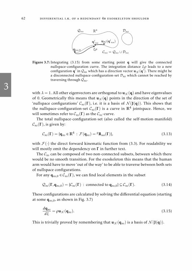
3
62 differential i.k. of a redundant 4r exoskeleton shoulder
qns,0
Qns R4
ξρ
q′
nsuN (q′
ns)
Dns
Cns = Qns ∪ Dns
Figure 3.7: Integrating (3.15) from some starting point q will give the connectednullspace-configuration curve. The integration distance ξρ leads to a newconfiguration q′ in Qns which has a direction vector uN (q′). There might bea disconnected nullspace-configuration-set Dns which cannot be reached bytraversing through Qns .
with λ = 1. All other eigenvectors are orthogonal to uN (q) and have eigenvalues
of 0. Geometrically this means that uN (q) points in the direction of the set of
‘nullspace configurations’ Cns(Γ), i.e. it is a basis of N (J(q)). This shows that
the nullspace-configuration-set Cns(Γ) is a curve in R4 jointspace. Hence, we
will sometimes refer to Cns(Γ) as the Cns-curve.The total nullspace-configuration-set (also called the self-motion-manifold)
Cns(Γ), is given by:
Cns(Γ) = qns ∈R4 : F (qns) =
gRua(Γ), (3.13)
with F (·) the direct forward kinematic function from (3.3). For readability we
will mostly omit the dependency on Γ in further text.
The Cns can be composed of two non-connected subsets, between which there
would be no smooth transition. For the exoskeleton this means that the human
arm would have to move ‘out of the way’ to be able to traverse between both sets
of nullspace configurations.
For any qns,0 ∈ Cns(Γ), we can find local elements in the subset
Qns(Γ,qns,0) = Cns(Γ) : connected to qns,0 ⊆ Cns(Γ). (3.14)
These configurations are calculated by solving the differential equation (starting
at some qns,0, as shown in Fig. 3.7)
dqns
dξ= ρuN (qns). (3.15)
This is trivially proved by remembering that uN (qns) is a basis ofN (J(q)).

3
3.3 preliminaries 63
The other ‘half’ of the Cns that is not reachable we call the disjointed region
Dns, defined as
Dns(Γ,qns,0) = Cns(Γ) \Qns(Γ,qns,0) ⊂ Cns(Γ). (3.16)
For some Γ we have that Dns = ∅.
3.3.4 Properties of Cns
When plotting the Cns-curves through (3.15) we notice ‘regions’ in jointspace
with different ‘behavior’. The bounds of these regions (separatrices) appear to be
the Qns(qns,0)-curves of qns,0 that contain q2 = nπ,q3 = mπ, ∀n,m ∈ Z (q1 and
q4 values do not matter). The separatrices pass through rank-2 (fully singular)
configurations. Therefore we will call these bounds singularity-separatrices.
The singularity-separatrices can be projected on the q2-q3-plane, as shown in
Fig. 3.8a. Investigation shows six regions of nullspace-configuration curves that
show three different kinds of behavior, dependent on values of Φ.
The regions and behaviors for our specific design are as follows (neglecting
q4, because it is only linked to axial rotation of the arm):
• Type Ia and Ib solutions: two disjointed closed loops Qns and Dns in q2-q3but continuously connected in q1. The total shape is helical.
• Type IIa and IIb solution: a single (i.e. Dns = ∅) complete closed loop Cnsin q1-q2-q3.
• Type III solution: two disjointed curves Qns and Dns, continuously con-
nected in q1-q2, but limited in domain in q3.
Typical projected-solutions for all three types of Cns-curves are shown in Fig. 3.9
The singularity-separatrices have a clear meaning when considering the human
arm-movement. They are elevation circles on the elbow-sphere, but rotated over
two angles Θ. The circles are at relative elevation angles (relative to the rotated
north- and south-‘poles’ on the sphere) 15, 75, 105 and 165 (dependent onΦ). This gives 5 regions for Ia, IIa, III, IIb and Ib solution types. An illustration
of these circles is given in Fig. 3.8b.
We can draw several conclusions from the separatrix-planes and the nullspace-
configuration-curves:
1. It shows that the gimbal system can only become singular when the arm
is on such a curve and almost singular when close to such a curve. Hence,

3
64 differential i.k. of a redundant 4r exoskeleton shoulder
0
π/2
π
3π/2
2π
0 π/2 π 3π/2 2πq2 [rad]
q 3[rad
]Ia
Ia
IIa
IIa
IIb
IIb
III
III
Ib
Ib
Singularity-Separatrices
(a)
zg xg
yg
Ib
Ia
IIbIIa
III
Elbow-Tip
(b)
Figure 3.8: a) Singularity-separatrices: The q2-q3 plane showing the conditioningand moving arm collision constraints. Superimposed are the singularity-separatrices in which nullspace-configurations curves will always stay. Eachregion is numbered dependent on the type of behavior of the curve. It can beseen that the Ib region always overlaps with the collision of the upper armwith the first motor. It should be noted that the space repeats itself every 2πrad. b) The human elbow-tip can reach points on a sphere. On this sphere,the nullspace-separatrices are circles (magenta). Only if the elbow is on sucha circle, the exoskeleton can possibly become fully singular. The elbow-tippoint is illustrated at the bottom of the sphere.
we are only in danger of poor conditioning close to these curves, and we
can focus more on collision avoidance outside of these neighborhoods.
2. The IIa and IIb solutions are the only ones that have Dns = ∅. Hence, if we
want to traverse between disjointed regions in Ia, Ib or III, we could do so
through IIa or IIb.
3. On purpose we placed the Ib solution region outside of the human-workspace,
since that region will always overlap with the collision of the human arm
with the first motor.

3
3.4 proposed inverse kinematics method 65
0
π/2
π
3π/2
2π
0 π/2 π 3π/2 2πq1 [rad]
q 2[rad]
Typical Nullspace-Configuration-Sets
IIIIII
(a)
0
π/2
π
3π/2
2π
0 π/2 π 3π/2 2πq2 [rad]
q 3[rad]
Typical Nullspace-Configuration-Sets
IIIIII
(b)
Figure 3.9: Typical shapes of null-space-configuration sets, a) q1-q2-plane b) q2-q3-plane.The shapes are invariant to q1 and q4, but will translate along the q2-q3 viewif q1 changes. The separatrices are shown as magenta colored dashed lines.
3.4 proposed inverse kinematics method
We require a method that uses (3.8), the minimum norm velocities in combina-
tion with nullspace velocities, to move to a configuration that still satisfies (3.4),
but should not violate any collision or conditioning constraint.
A candidate solution is gradient projection of the form
qns = P(q)∇f (q), (3.17)
with P(q) the projector described in (3.11), f (q) a scalar potential function with
a global minimum (global in the sense of a 2π repeating space would imply it is
local in a hypercube, but there is only a single potential minimum in such a hy-
percube) in R4 dependent on exoskeleton conditioning and collision avoidance.
The gradient projection method, in general, finds only locally optimal config-
urations in Qns since convergence ends when uN (q) and ∇f (q) are orthogonal.
The Qns is a highly complex function of q. To have more control over what con-
figuration the exoskeleton converges to, a single global minimum on Qns would
have to be constructed with the function f (q) to apply (3.17).
Generating the potential f (q) to accomplish this task is very difficult, in gen-
eral, because it requires full knowledge and parameterization of Qns. Therefore,
we relieve this difficulty by designing a potential on the 1D Qns. We can then
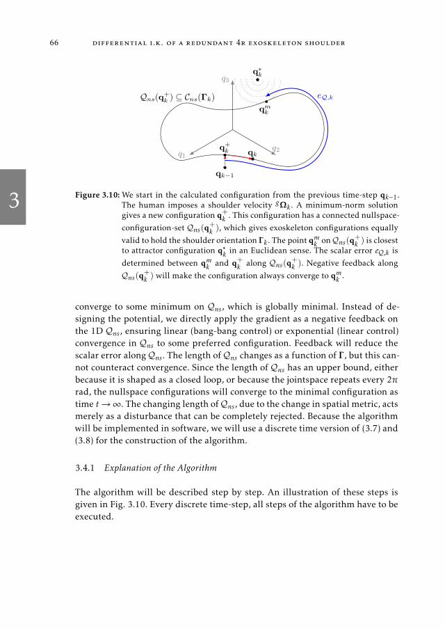
3
66 differential i.k. of a redundant 4r exoskeleton shoulder
q1q2
q3
eQ,kQns(q+
k ) ⊆ Cns(Γk)
qk−1
q+
k qk
q∗
k
qmk
Figure 3.10:We start in the calculated configuration from the previous time-step qk−1.The human imposes a shoulder velocity gΩk . A minimum-norm solutiongives a new configuration q+k . This configuration has a connected nullspace-
configuration-set Qns(q+k ), which gives exoskeleton configurations equally
valid to hold the shoulder orientation Γk . The point qmk onQns(q+k ) is closest
to attractor configuration q∗k in an Euclidean sense. The scalar error eQ,k is
determined between qmk and q+k along Qns(q+k ). Negative feedback along
Qns(q+k ) will make the configuration always converge to qmk .
converge to some minimum on Qns, which is globally minimal. Instead of de-
signing the potential, we directly apply the gradient as a negative feedback on
the 1D Qns, ensuring linear (bang-bang control) or exponential (linear control)
convergence in Qns to some preferred configuration. Feedback will reduce the
scalar error along Qns. The length of Qns changes as a function of Γ, but this can-
not counteract convergence. Since the length of Qns has an upper bound, either
because it is shaped as a closed loop, or because the jointspace repeats every 2π
rad, the nullspace configurations will converge to the minimal configuration as
time t→∞. The changing length ofQns, due to the change in spatial metric, acts
merely as a disturbance that can be completely rejected. Because the algorithm
will be implemented in software, we will use a discrete time version of (3.7) and
(3.8) for the construction of the algorithm.
3.4.1 Explanation of the Algorithm
The algorithm will be described step by step. An illustration of these steps is
given in Fig. 3.10. Every discrete time-step, all steps of the algorithm have to be
executed.
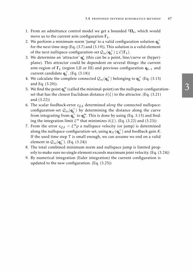
3
3.4 proposed inverse kinematics method 67
1. From an admittance control model we get a bounded gΩk , which would
move us to the current arm configuration Γk .
2. We perform a minimum-norm ‘jump’ to a valid configuration solution q+kfor the next time step (Eq. (3.7) and (3.19)). This solution is a valid element
of the next nullspace-configuration-set Qns(q+k ) ⊆ C(Γk).
3. We determine an ‘attractor’ q∗k (this can be a point, line/curve or (hyper)-
plane). This attractor could be dependent on several things: the current
arm-region of Γk (region I,II or III) and previous configuration qk−1 and
current candidate q+k . (Eq. (3.18))
4. We calculate the complete connected Qns(q+k ) belonging to q+k (Eq. (3.15)
and Eq. (3.20)).
5. We find the point qmk (called theminimal-point) on the nullspace-configuration-
set that has the closest Euclidean distance δ(ξ) to the attractor. (Eq. (3.21)
and (3.22))
6. The scalar feedback-error eQ,k determined along the connected nullspace-
configuration-set Qns(q+k ) by determining the distance along the curve
from integrating from q+k to qmk . This is done by using (Eq. 3.15) and find-
ing the integration limit ξm that minimizes δ(ξ). (Eq. (3.22) and (3.23))
7. From the error eQ,k = ξmρ a nullspace velocity (or jump) is determined
along the nullspace-configuration-set, using uN (q+k ) and feedback gain K .
If the used time step T is small enough, we can assume we end on a valid
element in Qns(q+k ). (Eq. (3.24))
8. The total combined minimum-norm and nullspace jump is limited prop-
erly tomake sure no single element exceedsmaximum joint velocity. (Eq. (3.24))
9. By numerical integration (Euler integration) the current configuration is
updated to the new configuration. (Eq. (3.25))
3
68 differential i.k. of a redundant 4r exoskeleton shoulder
The algorithm is summarized as follows:
q∗k = f (qk−1,Γk) (3.18)
q+k = qk−1 + T J†(qk−1)gΩk (3.19)
Qns(q+k ) = use Eq. (3.14) and Eq. (3.15) (3.20)
δ(ξ) = Eucl. dist. betw. q∗k and Qns(q+k ) (3.21)
ξm = argminξ∈R
δ(ξ) (3.22)
eQ,k = ξmρ (3.23)
qk = sat[J†(qk−1)gΩk −KeQ,kuσ (q
+)] (3.24)
qk = qk−1 + T qk , (3.25)
with T the sample time of the algorithm and sat[·] a proper saturation function
based on the maximum element. Some practical remarks on this algorithm can
be found in the supplementary material.
Instead of solving the difficult problem of designing a potential function f (q)
for gradient projection, we have changed the problem to 1) choosing a simple
q∗k , and 2) executing a computationally more intensive task of calculating parts
of Qns(q+k ) using Eq. (3.14) and Eq. (3.15).
3.4.2 Choosing Attractor q∗k
The challenge in the current method lies in generating an attractor q∗k . We have
to generate an attractor that ensures (in combination with feedback) the solu-
tions to stay away from collision and poor conditioning. We pick a possible sim-
ple choice, valid for our design choices Φ, Θ and geometry. In our case, the at-
tractor is a hyper-plane described by the implicit plane equation (q2−0.6π) = 0,
meaning q1, q3, q4 can take any value. Choosing this hyper-plane ensures attrac-
tion of q2 to 0.6π rad, staying away from body collisions and poor conditioning.
If the value of 0.6π cannot be achieved for q2 (either it is not a valid element of
the connected Qns, or it would violate the velocity constraints), it will try to be
‘close’. Our attractor is invariant to the solution-region and arm/joint velocities,
although it need not be.
We want to emphasize that this choice for q∗k may not be the best, but is used
to show that the problem can now be solved, even with a simple choice for the
3
3.4 proposed inverse kinematics method 69
attractor. A better, more dynamic, attractor could try to improve exoskeleton
conditioning to achieve lower joint velocities.
3.4.3 Claims of Quasi-Static Convergence
An informal proof of convergence of our method is given in a quasi-static sense,
i.e. when the exoskeleton starts in a configuration conforming to constraints,
not obstructed by constraints, and the human moves infinitely slowly (or: the
feedback gain is higher than the human movement speed). In this way, the IK
method converges to the minimal point qmk . This ‘theorem’ can be used after-
wards to find conditions for dynamic convergence in Sec. 3.4.4.
First, we denote all possible null-space-configurations in Qns that are accessi-
ble or allowed (because they do not violate a conditioning or collision constraint),
and are directly connected to our current configuration qk as the allowed com-
pact subset:
Ans(Γ,qk) = qns ∈ Qns(Γ,qk) : conforming to constraints. (3.26)
Such subsets we call ‘Ans-loops’.
Secondly, we need two prerequisites to make any convergence claims:
Prerequisite 1: The rotational velocity gΩ of the shoulder, imposed by the
human, is bounded. We assume a finite L2 norm of ‖gΩmax‖2.Prerequisite 2: The rotations of the arm Γ are always element of a smaller
compact set, the human workspace Wh, than the complete set of all rotations,
i.e. Γ ∈Wh ⊂ SO(3).
Prerequisite 1 is required, otherwise a quasi-static proof of convergence has
no value. Prerequisite 2 is required, because vanishing Ans-loops do occur out-
side of the human workspace (see more explanation about vanishing Ans-loops
in Claim 2 below), which would be problematic.
Consequently, we make the following claims which, if they all hold, ensure
the system never violates conditioning and collision constraints in a quasi-static
sense.
Claim 1: For any arm configuration there is always a minimal point qmk that
does not violate any constraint.
Claim 2: The minimal point qmk is never inside a Ans-loop that vanishes com-
pletely into a constraint (i.e. Ans(Γ,qns) = ∅) for ‘some (unknown) worst arm
motion’ gΩ that would make this Ans-loop vanish.
3
70 differential i.k. of a redundant 4r exoskeleton shoulder
The proof is informal since both claims can only be shown to be true by vi-
sual inspection. Claim 1 is achieved by proper choice of q∗k . It holds, since the
hyperplane q∗k = 0.6π intersects withQns always in region III, and for part of the
arm configurations in regions IIa and IIb. If the plane does not intersect, the pro-
jected shape of Qns onto q1-q2 in the region q2 ∈ [0,π] is fully convex outside the
constraints in regions IIa, IIb and Ia. Therefore, there is a single minimal point
conforming to all constraints. The region Ib has no feasible solutions by design,
due to motor 1 collision, and is placed outside of Wh, and is not a problem.
Claim 2 is achieved by by proper design choices of Φ, Θ. It holds because: a)
In region Ia, no arm movement gΩ can make the Ans-loop vanish. b) Similarly,
for the part of the IIa region, there is no possibility for an Ans-loop to vanish
into a constraint. c) In region III and parts of IIa and IIb, the projected shape
of Qns is almost diagonal across the q1 − q2 plane. Therefore, there is always an
intersecting solution qmk = q∗k . d) In region IIb, the only remaining Ans-loop al-
most vanishes when approaching region Ib, but it never does. Although solution
spaceAns becomes small, it remains convex in projection on q1−q2, with a single
qmk .
3.4.4 Condition for Dynamic Convergence
Given the claims that the method will quasi-statically converge, it is possible to
derive sufficient conditions for convergence in a dynamic sense.
The differential kinematics from (3.5), can be rewritten by performing an a
singular value decomposition as follows:
gΩ = J(q)q= UΣVT q,
with
Σ = [diag([σ1,σ2,σ3]) 03].
Then the minimum norm solution to (3.7) is described by
qmn = J†(q)gΩ = VΣ+UT g
Ω,

3
3.4 proposed inverse kinematics method 71
with
Σ+ =
diag([σ−11 ,σ−12 ,σ−13 ])
0T3
. (3.27)
In (3.27), σ−1j (j = 1,2,3) are the principal axes of the ellipsoid formed by the
singular values of J†(q). This ellipsoid governs the scaling of the input vector gΩ
to the jointspace. If we set σmin =min ([σ1,σ2,σ3]), the minimum norm solution
is always within a sphere with the largest ellipsoid radius σ−1min:
∥∥∥gΩmaxσ
−1min
∥∥∥2≥
∥∥∥qmn,max
∥∥∥2.
This holds because V, U and its transposes are unitary and do not scale vectors.
The minimum-norm solution can drop the new configuration anywhere in-
side, or onto, the sphere. In a worst case, this is exactly∥∥∥gΩmaxσ
−1min
∥∥∥2T away
from the minimal point qmk . Therefore, we need the nullspace-velocity-norm to
be greater than the minimum-norm to bring us always closer towards qmk along
Qns.
To achieve this, we need that
‖qns‖2 ≥∥∥∥gΩmaxσ
−1min
∥∥∥2.
Due to our design choices, this is equivalent to
∥∥∥uNKeQ
∥∥∥2≥
∥∥∥gΩmaxσ
−1min
∥∥∥2.
Since ‖uN ‖2 = 1 and by defaultK ≥ 0 and σmin ≥ 0, we can rewrite this condition
as
K |eQ| ≥ ‖gΩmax‖2σ−1min.
Which gives as condition for our feedback gain:
K ≥ ‖gΩmax‖2|eQ|
σ−1min, (3.28)

3
72 differential i.k. of a redundant 4r exoskeleton shoulder
Figure 3.11: Benchmark armmovement. The arm starts in the zero configuration at t = 0s. All sequential poses are shown at time intervals of 0.5 s.
such that a valid nullspace velocity solution condition for dynamic convergence
is
qns ≥ ‖gΩmax‖2σ−1minsgn(eQ)uN . (3.29)
This nullspace velocity ensures a net convergence as discrete time k→∞. It also
gives a maximally allowed arm velocity, dependent on exoskeleton joint motor
capabilities.
Instead of the sgn(x)-function, an alternative is the use of the tanh (βx), since
limβ→∞ tanh (βx) = sgn(x). This ensures smoother behavior for small eQ, aslong as for errors greater than approximately 0.1 rad tanh (β|eQ|) ≈ 1, we still
have guaranteed convergence before hitting any constraint surface.
Also, to be less conservative, instead of ‖gΩmax‖2 in (3.29), it is possible to use
‖gΩk‖2 of the current time step.

3
3.5 results 73
01
23
45
6−2
π−π0π
2π
time[s]
angularvel.[rad/s]
Referen
ceMotion
gΩ
xgΩ
ygΩ
z
(a)
01
23
45
6−2
π−π0π
2π
time[s]
angularvel.[rad/s]
JointAng.Vel.3R-Y
XY
q 1q 2
q 3
(b)
01
23
45
6−2
π−π0π
2π
time[s]
angularvel.[rad/s]
JointAng.Vel.3R-X
ZY
q 1q 2
q 3
(c)
01
23
45
6−2
π−π0π
2π
time[s]
angularvel.[rad/s]
JointAng.Vel.3R-Y
XZ
q 1q 2
q 3
(d)
01
23
45
6−2
π−π0π
2π
time[s]
angularvel.[rad/s]
JointAng.Vel.New
4R
q 1q 2
q 3q 4
(e)
01
23
45
60π
2π
3π
time[s]
angle[rad]
JointAnglesNew
4R
q 1q 2
q 3q 4
(f)
Figure
3.12:R
eferen
cemotionofthearm
andresu
ltingexoskeletonvelocities
(3R+4R)an
dan
gles(4Ronly).a)
Aminim
aljerk
reference
motionin
shoulder
rotation,asdescribed
inthetext.b-e)Theresu
ltingexoskeletonjointvelocities
fora
3R-Y
XY,3R-X
ZY
and3R-Y
XZdesignsresp
ectively.Note
that
thevelocities
goto
infinitymultiple
times
dueto
poorconditioningofthe3Rjoints.Thelegen
din
(c)also
reflects
thejoints
in(b)an
d(d).e-f)Thejointvelocities
andan
gles,resp
ectively,ofthenew
4Rdesign.Thesystem
never
becomes
singular,althoughjointsp
eedslooka
bithigher
than
3Rdesignsonaverag
e.The4Rjointan
glesalso
stay
inacompactlimited
range.
Thisis
insharp
contrastto
the3R
designs,
wherehighvelocities
resu
ltin
largejointrange(andtherefore
possibly
man
ybody
collisions).

3
74 differential i.k. of a redundant 4r exoskeleton shoulder
0 1 2 3 4 5 60
0.25
0.5
0.75
1
time [s]
conditioning[−]
Joint Conditioning
4R3R-YXY3R-XZY3R-YXZ
Figure 3.13: Conditioning of the 4R and 3R exoskeletons. The 3R exoskeletons have poorconditioning at certain arm configurations. The 4R system manages to havebetter overall conditioning, which helps in avoiding excessive joint veloc-ities. The fact that the maximal conditioning is a bit less than for all 3Rexoskeletons, is because the 4R exoskeleton is non-orthogonal.
3.5 results
3.5.1 Analytical Benchmark
In this section we show a validation of the method by following an analytical
benchmark movement with the new 4R design. The conditioning and joint ve-
locities are compared to common orthogonal 3R exoskeleton architectures given
by rotation orders YXY , XZY , YXZ (stating the exoskeleton axis direction in
the human’s zero-pose), as is shown in [44] (see Chapter 2, Sec. 2.2.1 and 2.2.2).
We did not generate geometry for the 3R designs and could therefore not
check for head, trunk and arm collisions in their case. We did, however, check
for head, trunk and arm collisions for the new 4R design, since it was a prereq-
uisite for the method to succeed and to be useful.
The benchmark motion is shown in Fig. 3.11 and Fig. 3.12a. It is composed of
local rotations, transformed to the global frame, to generate a global arm veloc-
ity gΩ. The benchmark motion is such that the 3R shoulders will pass through
their singular configurations, resulting in very large joint velocities, approach-
ing infinity.
The simulation for 3R and 4R was performed with T = 1 ms. The used 4R
IK method was the one in (3.29), but with tanh (5eQ) instead of sgn(eQ). InFig. 3.12b-d it is clearly visible that 3R shoulders all have troubling configu-
rations at which singularity occurs, while the movement is within the human
workspace. At these configurations the joint conditioning of the 3R designs be-

3
3.5 results 75
(a)
(b)
Figure 3.14: a) The used 1:2 scale setup shown conceptually in Fig. 3.1 and detailed inTable 3.1. Four brushed DC motors drive the four DOF. The setup has a sin-gle CoR where all joint axes intersect. b) From left to right: a self-motion ofthe joint, frames spaced approximately 0.3 s apart. Note that the arm hardlymoves during self-motion of the joint. Any residual motion is due to incre-mental encoder angle calibration error and play in the motor transmission.
comes very poor, while the 4R design actively attempts to continually achieve
proper conditioning (see Fig. 3.13).
3.5.2 Test Setup
A 1:2 scale test setup, shown conceptually in Fig. 3.1 and detailed in Table 3.1,
is shown in Fig. 3.14. The four DOF are driven by Pololu D37 brushed DC mo-
tors with transmission ratios of 1:70, 1:50, 1:50, 1:19 for motors actuating axes
ω1 to ω4 respectively. All four motors have 64 incremental encoder counts per

3
76 differential i.k. of a redundant 4r exoskeleton shoulder
05
10
15
20
25
−π
−12π 0
12π π
time[ s]
angular vel. [rad/s]
Referen
ceMotio
n
gΩ
xgΩ
ygΩ
z
(a)
05
10
15
20
25
−32π
−π
−12π 0
12π π
32π
time[ s]
angular vel. [rad/s]
JointAng.Vel.
New
4R
q1
q2
q3
q4
(b)
05
10
15
20
25
0
12π π
32π
2π
time[ s]
angle [rad]
JointAngles
New
4R
q1
q2
q3
q4
(c)
05
10
15
20
25
−π
−12π 0
12π π
time[ s]
angular vel. [rad/s]
Minim
um-N
orm
Contrib
.qmn,1
qmn,2
qmn,3
qmn,4
(d)
05
10
15
20
25
−π
−12π 0
12π π
time[ s]
angular vel. [rad/s]
Nullsp
aceVel.
Contrib
utio
nqns,1
qns,2
qns,3
qns,4
(e)
05
10
15
20
25
10 −
4
10 −
3
10 −
2
time[ s]
calc. time [s]
Calcu
lationTim
e
(f)
Figure
3.15:R
eference
motio
nofthearm
andresu
ltingexoskeleto
nvelo
citiesan
dan
gles.
a)A
reference
motio
ngΩ
given
by
ahuman
operato
rin
real-timebya3-ax
isjoystick
.b)Theresu
ltingjointvelo
citiesfro
mtheIK
meth
od.c)
The
resultin
gan
gles
from
theIK-m
ethod.Thedash
edlin
esindicate
thecalcu
latedan
gles.
Thesolid
lines
indicate
measu
redan
gles
ofthesetu
p.Angles
wrap
aroundat
0an
d2π
radd)theminim
um
norm
contrib
utio
nto
the
jointvelo
citye)
thenullsp
acecontrib
utio
nto
thejointvelo
cityf)req
uired
calculatio
ntim
eforthemeth
odona
single
core
ofa0.8–2.0
GHzIntel
5Y10processo
r.

3
3.5 results 77
0 5 10 15 20 250
0.25
0.5
0.75
1
time [s]
conditioning[−]
Joint Conditioning
Figure 3.16: Conditioning of the 4R test setup during the motion.
motor revolution. The motors are driven with two Pololu VNH5019 Dual motor
drivers with 9 V power supply. Low-level PID joint angle control runs at an up-
date frequency of 1000 Hz and is implemented on an NXP FRDM K64F board
(MK64FN1M0VLL12 microcontroller, running at 120 MHz) that sends PWM
signals to the motor drivers. Instead of a force/torque sensor, the deflection of
a 3-axis joystick (pitch, roll and yaw) is used to determine global arm velocitygΩ. In a full size exoskeleton a force/torque sensor on the exoskeleton would
measure human operator forces/torques. These torques would generate a local
angular acceleration that would be integrated and transformed to a velocity vec-
tor expressed in the global frame. A 3D-printed 1:2 scale human arm is attached
to be able to visualize axial arm configuration.
The IK algorithm used is the same as in Sec. 3.5.1. Code used to calculate
results in Sec. 3.5.1 is compiled to a Matlab executable in Matlab 2015b on
Microsoft Windows 10. This allows for single-threaded IK computations on a
single core of a 0.8–2.0 GHz Intel 5Y10 Dual-Core M processor. Calculated ref-
erence joint angles from the IK method are transmitted from Matlab over USB
to the microcontroller at a rate of 50 Hz.
The arm started in the human’s zero-pose. A human operator gave a real-time
desired arm velocity, in the global frame, to the system by moving the 3-axis
joystick (see Fig. 3.15a). The resultingmotion of the setup is shown in Fig. 3.15b–
c. The contribution of the minimum-norm solution and the added nullspace
contribution is shown in Fig. 3.15d–e. It shows that the minimum-norm and
nullspace solution have opposite signs when moving joint q2. The software used
in the setup checks whether it would violate any of the jointspace constraints
outlined in Sec. 3.3.1 and would then stop the motion. This did, however, not

3
78 differential i.k. of a redundant 4r exoskeleton shoulder
happen during the testing motion. Conditioning of the joint was above 0.6, as is
shown in Fig. 3.16, similar to results in Fig. 3.13.
Computationally, the method was sufficient for real-time applications, as is
shown in see Fig. 3.15f. Calculation times were up to 3 ms in the worst case,
allowing for a kinematic update frequency above 300 Hz. Longer calculation
times up to 3 ms are required when Qns does not intersect the hyper-plane q2 =
0, because the integration of the self-motion-manifold (see Eq. (3.20)) cannot be
terminated prematurely. The largest timing bottleneck in this setup is the used
data-communication method between PC and microcontroller and not in the
practical implementation of the proposed IK method in this work.
The results show that the method is applicable in real-time applications. For
full scale exoskeletons the method would be implemented in dedicated real-
time software. This transition would allow for shorter calculation times and
a faster communication with low-level joint controllers, allowing for more up-
dates of the joint angle reference trajectories.
3.6 discussion and conclusion
In this chapter we have studied the kinematic design and a new differential IK
algorithm for a 4R exoskeleton shoulder joint.We ensure convergence to a global
(in the sense of repeating space) minimum on the nullspace configuration sets to
avoid body collisions and have proper exoskeleton conditioning. By identifying
a preferred, but not enforced, configuration (the attractor), we have outlined a
method to always converge on the nullspace configuration set through linear or
bang-bang negative feedback to a configuration closest (in an Euclidian sense)
in jointspace.
Results show that this exoskeleton, combinedwith the algorithm, outperforms
standard 3R joints in terms of conditioning. The joint velocities of the 4R are
similar to 3R in an absolute average sense. Still, 3R designs demanded infinite
velocities within the used benchmark motion. Also, collisions with the body and
arm were fully avoided in the 4R case, but could not be tested for the 3R cases.
If the method has to be applied in the acceleration domain, one has to use
higher order integration methods (such as Runge-Kutta) to avoid large numer-
ical drift when traversing Qns. This adds an extra layer of complexity we have
now avoided. Furthermore, there would be the need for critically damped pro-
portional and derivative negative feedback.

3
3.6 discussion and conclusion 79
The presented method is limited by the fact that solutions are found in the
velocity domain instead of the acceleration domain. This may result in non-
smooth velocity profiles, imposing possibly infinite joint accelerations. In prac-
tice, this is a minor problem. Because admittance dynamics models are first or-
der from force to velocities, the joint velocities are mostly always smooth.
Further limitation of any 4R shoulder exoskeleton, regardless of the control
method and inverse kinematics method used, is the inherent safety problem
considering the lack of mechanical joint limits. This problem is also present in
several 3R exoskeletons, albeit to a lesser extent. Software imposed joint limits
can be used, but these are inherently less safe than mechanical end-stops.


Part II
HAPTICS & CONTROL :ADMITTANCE CONTROL


4
4ADMITTANCE CONTROL FOR PHYS ICAL HUMAN-ROBOT
INTERACT ION
Arvid Q.L. Keemink, Herman van der Kooij and Arno H.A. Stienen
You push with the heel of your hand; the suit feels it, amplifies it, pushes with
you to take the pressure off the receptors that gave the order to push. [...] The
suit has feedback which causes it to match any motion you make, exactly – but
with great force. Controlled force... force controlled without your having to
think about it.
— Robert Heinlein, Starship Troopers, 1959
Abstract–This chapter presents an overview of admittance control as amethod
of physical interaction control betweenmachines and humans.We present an
admittance controller framework and elaborate control scheme that can be
used for controller design and development. Within this framework, we ana-
lyze the influence of feed-forward control, post-sensor inertia compensation,
force signal filtering, additional phase lead on the motion reference, internal
robot flexibility, which also relates to series elastic control, motion loop band-
width and the addition of virtual damping on the stability, passivity and per-
formance of minimal inertia rendering admittance control. We present seven
design guidelines for achieving high performance admittance controlled de-
vices that can render low inertia, while aspiring coupled stability and proper
disturbance rejection.
list of used symbols and abbreviations
Symbol Explanation
a subscript: relating to apparent dynamics transfer function or accel-
eration
app subscript: relating to apparent dynamic property
This chapter is accepted to be published in the International Journal of Robotics Research(IJRR).
83

4
84 admittance control for physical human-robot interaction
b physical or virtual generalized damping coefficient
c subscript: relating to the controller
C controller transfer function
d subscript: relating to the desired tracked trajectory
D transfer function denominator
ext subscript: relating to external input force
f subscript: relating to force
fb subscript: relating to feedback control
ff subscript: relating to feed-forward control
F physical or virtual mechanical force or torque
gf subscript: relating to force gain
G controller gain
h subscript: relating to a human’s mechanical property
H generic transfer function
i electrical current
subscript: relating to electrical current, or integral gain
int intrinsic dynamical property of the human limb
I(·) imaginary part of the argument
j imaginary constant√−1
k physical or virtual mechanical stiffness, controller gain or transmis-
sion ratio
K controller gain amplified by transmission ratio
m physical or virtual mechanical generalized inertia
subscript: relating to the actuator (motor)
n Butterworth filter polynomial order
N transfer function numerator
ps subscript: post-sensor effect
r subscript: relating to robot or gearing ratio
R set of all real numbers
R(·) real part of the argument
s laplace variable
subscript: relating to sampling time or structural stiffness
smp Discrete time sampler

4
admittance control for physical human-robot interaction 85
S sensor or state/signal estimator transfer function
t subscript: relating to target dynamics
T delay time
subscript: relating to torque
v physical or virtual mechanical velocity or angular velocity
subscript: relating to the virtual dynamics parameters, virtual dy-
namics transfer functions or velocity
Y mechanical admittance, either virtual or physical
Y baseline system admittance
πY mechanical admittance that is guaranteed to be passive
Z mechanical impedance, physical
Z mechanical impedance, model
β feed-forward mechanical linear or rotational damping
γ mass fraction between 0 and 1
µ feed-forward mechanical linear mass or rotational inertia
τ first order dynamical system time constant
ω angular frequency
Abbrev. Explanation
4C four channel
CVT continuous variable transformer
DA digital-to-analog
DOF degree of freedom
ez-width environment z-width
LTI linear time invariant
NAC natural admittance control
PD proportional-derivative
PDD2 proportional-derivative-double-derivative
pHRI physical human robot interaction
PI proportional-integral
PID proportional-integral-derivative
ZOH zero-order-hold
4
86 admittance control for physical human-robot interaction
4.1 introduction
During physical human-robot interaction (pHRI) a robot measures motions of
or forces from the human and adequately responds to these. Several control
methods exist for controlling robots in contact with a mechanical environment
[59], namely: (in)direct force control [60], impedance control [61], admittance
control [62, 63] and full-state interaction control [64, 65]. The human user is
usually seen as a special case of the environment.
In this chapter we discuss the admittance control paradigm, a control method
that is not commonly used for haptic interaction control [66]. By measuring
the interaction force with the human user, the set-point to a low-level motion-
controller is changed through virtual model dynamics to achieve some preferred
interaction responsive behavior [62, 60, 67] (see Fig. 4.1). The motion controller
is commonly a reference following velocity controller, due to power conjugation
of force and velocity, and this is what we will assume in the remainder of the
text.
Bymaking the relation between themeasured force and the velocity-reference,
the virtual model dynamics, consistent with laws of mechanics, simulation of
physical dynamical systems is possible [68, 69].
Admittance control is the opposite, or dual [68, 67], of impedance control
[61]. During impedance control forces are applied, either through open loop or
closed loop control, to the human user after device motion is measured. The
naming reflects the causality of the used virtual model dynamics. Due to this
dual nature of admittance control and impedance control, they naturally excel
at both different ends of the ‘haptic spectrum’ [70, 68, 66, 71]. For admittance
controlled devices it is easier to render stiff virtual surfaces and a challenge
to render low inertia. It is troubled by dynamically interacting with stiff real
surfaces (constrainedmotion) [72, 73, 68]. Impedance control, on the other hand,
is a better candidate to render low inertia but not to render stiff virtual surfaces.
It is troubled by dynamically interacting with low inertia (free motion) [68].
4.2 motivation
Although admittance control has been successfully applied in multiple devices
(see Sec. 4.3.2), an overview of applications, properties and possibilities of ad-
mittance control is lacking. We provide an overview of the development and
applications of admittance control. In addition, we briefly recapitulate the no-

4
4.3 background 87
Yv C YrFext vd e Fc v
−
Figure 4.1: Basic stand-alone admittance control diagram of an uncoupled admittancecontrolled robot. It shows the measured externally applied force Fext, pass-ing through the virtual dynamics Yv to generate velocity reference vd . A con-troller C attempts to enforce this velocity on the robot Yr by applying a con-trol force Fc through an actuator (not shown). External force Fext also actsdirectly on the robot dynamics Yr . The resulting motion of the robot is givenby v.
tions of stability and passivity of admittance controlled systems. The main con-
tribution of this work is the presentation of an elaborate admittance controller
framework and its control scheme that summarizes major contributions from
literature and experience, which can be used for controller design and devel-
opment. Within this framework, we analyze the influence of 1) feed-forward
control, 2) force signal filtering, 3) post-sensor inertia compensation, 4) the ad-
dition of virtual damping, 5) additional phase lead on the motion reference, 6)
motion loop bandwidth, and 7) internal robot flexibility (which in the limit di-
rectly relates to series elastic control) on the stability, passivity and performance
of minimal inertia rendering admittance control. Finally, these analyses lead to
a set of design guidelines for achieving high performance admittance controlled
devices that can render low inertia, aspiring robust coupled stability. The anal-
yses are focus solely on single-DOF, single interface linear time invariant (LTI)
systems with one-port admittance interaction only.
4.3 background
4.3.1 Naming
The name admittance control dates back to 1992 due to the developments of New-
man and Gullapalli et al. [63, 74] and Schimmels and Peshkin [75]. Different
names for what is commonly called admittance control can be found in litera-
ture: position based or velocity based impedance control [76, 77, 78, 79, 80, 81] and
[82] respectively. It is sometimes interchanged with impedance control [83, 84].

4
88 admittance control for physical human-robot interaction
In all cases there is the measurement of force that generates a motion control
reference or a deviation from such a reference.
Some authors distinguish between motion-based impedance control and ad-
mittance control by focusing in the former case on motion tracking and in the
latter case on force tracking [85, 59, 86].We choose to use the generic term admit-
tance control for all types of force-to-desired-motion relationships in this work,
and recognize the fact that an admittance controller can track both motion and
forces simultaneously.
The desired dynamical behavior, the admittance, felt at the ‘interaction port’
where the human interacts with the device, is called by different names: desired
dynamics [87], target dynamics [87, 88], mechanical drive point mobility [63], vir-
tual admittance/environment/model/dynamics [68, 67] or driving-point dynamics
[89]. It could also be called the indirect force controller.
Dependent on the form of the desired dynamical behavior, several authors
adopt different naming for the controller. The term admittance control is used for
a inertia simulation [67], but also for pure damping [90, 91] or generic force to
motion simulation [70, 68]. Accommodation control is solely used for pure damp-
ing behavior [62, 63]. Finally, compliance control is used for pure spring behavior
[59]. If the controller is to mask only (static) friction effects and keep the same
inertia (its natural admittance) as the robot system, Newman and Zhang [72]
proposed the name Natural Admittance Control (NAC).
In this work, we take the aforementioned single analyses, and the major inno-
vations and combine them into a single framework. We will use the term virtual
dynamics (or virtual admittance) to describe the dynamics we want the device
to display to the human, and to refer to the model that is used to calculate a ve-
locity reference for a velocity controller to track. The dynamics that are actually
felt by the human will be called the apparent dynamics (or apparent admittance),
which preferably approaches the virtual dynamics.
4.3.2 History and Applications
Interaction control gained widespread academic interest after the pioneering
work of Hogan [61] and Colgate [92] on impedance control and passivity at the
end of the 1980s. The first mentions of using a control method very similar to
admittance control date back to Whitney [62], where it was used to respond to
hard contact in industrial applications and therefore for indirect force control
purposes.

4
4.3 background 89
Initially, interaction control was developed for applications such as welding
and deburring, where stiff robot position control was highly impractical due to
high stiffness and friction of the processed parts [62, 77, 75, 93, 85]. Accom-
modation and admittance control were first introduced on retrofitted industrial
robots [62, 60, 77, 78, 94, 88]. Ott and Nakamura [81] exploit a force sensor in
the base to increase safety of the system. Bascetta et al. [95] use variable admit-
tance control for teaching of industrial manipulators to interact safely during
manufacturing.
A patent from Fokker Control Systems (US4398889 A) describes admittance
control in Flight Simulator devices in the field of control loading, starting from
1980. First mentions pHRI come from haptic master devices to render virtual
dynamics in flight simulation and later in more generic scenarios [96, 97, 98]. In
these cases virtual environments with admittance causality could be simulated,
allowing more straightforward rendering of constrained motions.
Mentions of active devices capable of safe interaction between human andma-
chines emerged at the beginning of the 1990s [99, 100]. Further development of
themethod led to successful practical admittance based devices such as the Hap-
ticMaster [69, 101] for generic haptic simulation, the Simodont for the training
of dental practice, and Lopes II [102] for the rehabilitation of human walking,
all developed by Moog Inc. [103].
Faulring et al. [104, 66] mention the use of Cobots with Continuous Variable
Transformers (CVTs) to be able to render stiff constraints in an admittance con-
trol mode. Other methods employ admittance control in a master slave setup
[105, 106] for surgery.
Exoskeleton control, used for the upper extremities [39, 107, 108, 109, 110],
is sometimes implemented as multi-DOF admittance-controlled devices to aid
in rehabilitation [111, 112, 45, 113, 114, 91]. Rendering low inertia and task
dependent stiffness assist the wearer in making motions with the arm. Due to
the motion-controlled nature of the device, it can switch seamlessly between
admittance control and pure motion-control. This makes it a good candidate
for identification of the human neuromusculoskeletal system dynamics through
applied position perturbations, and for switching between automated, reactive
and cooperative tasks, as explained by Stienen et al. [115].
Several lower extremity exoskeleton devices use admittance control to render
low impedance (high admittance) during the generation of locomotion patterns
for rehabilitation purposes [102, 116]. For mobile lower-extremity rehabilita-
tion the admittance controller is used to have carts move with the patient with

4
90 admittance control for physical human-robot interaction
minimal effort [117]. Other designs are developed for knee recovery specifically
[84, 118]. Amethod used by Aguirre-Ollinger et al. [84, 119] is to use admittance
control with acceleration feedback as implicit force control to reduce the inertia
of the lower leg of the human to facilitate knee recovery [13]. Rehabilitation of
the ankle with admittance control is described by Saglia et al. [120].
Admittance control for end-point interaction is mainly used for power ampli-
fication or load reduction [121, 122, 123, 124] and the masking of unwanted dy-
namical effects in industrial applications. In these cases the heavy-load bearing
capabilities of large and strong devices can result in substantial power amplifi-
cation of a human user.
Special cases of admittance control can be found for interaction with hu-
manoids [125, 126], anthropomorphic arms and hands [127], aerial vehicles
[128] and mobile carts [129].
Furthermore, learning and adapting admittance control schemes have been
implemented [74]. Adaptive models, time-varying parameters, or neural net-
works are used to optimize the interaction between the device and the human
towards some objective [130, 131, 132].
4.3.3 Design Challenges
Due to the velocity or position controlled nature of many admittance controlled
devices, it is straightforward to create stiff or dissipative haptic constraints to
assist in cooperative human-robot tasks. When the human is not supposed to
be constrained, the device should have high admittance (i.e. low impedance).
Preferably, the apparent admittance should be higher than the natural admit-
tance of the inert, heavy and dissipative robot.
Infinite admittance, or zero impedance, over the complete frequency range
is impossible to achieve on an admittance controlled device due to division by
zero in the force-velocity relationship. A common approach is to have the vir-
tual dynamics be a pure virtual inertia [84] that is as ‘low as possible’, while
retaining stability when coupled to the user. The pure virtual inertia assures
low impedance for low frequencies, attenuation of high frequencies and non-
dissipative behavior. The low virtual inertia admittance approach is the same as
high integral indirect force control with an inner velocity-control loop. The inte-
gral force gain is the reciprocal of the virtual inertia. Effectively, the low virtual
inertia generates a force controller that attempts to minimize the interaction
force between device and the user.
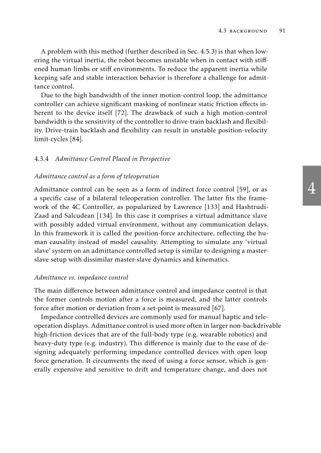
4
4.3 background 91
A problem with this method (further described in Sec. 4.5.3) is that when low-
ering the virtual inertia, the robot becomes unstable when in contact with stiff-
ened human limbs or stiff environments. To reduce the apparent inertia while
keeping safe and stable interaction behavior is therefore a challenge for admit-
tance control.
Due to the high bandwidth of the inner motion-control loop, the admittance
controller can achieve significant masking of nonlinear static friction effects in-
herent to the device itself [72]. The drawback of such a high motion-control
bandwidth is the sensitivity of the controller to drive-train backlash and flexibil-
ity. Drive-train backlash and flexibility can result in unstable position-velocity
limit-cycles [84].
4.3.4 Admittance Control Placed in Perspective
Admittance control as a form of teleoperation
Admittance control can be seen as a form of indirect force control [59], or as
a specific case of a bilateral teleoperation controller. The latter fits the frame-
work of the 4C Controller, as popularized by Lawrence [133] and Hashtrudi-
Zaad and Salcudean [134]. In this case it comprises a virtual admittance slave
with possibly added virtual environment, without any communication delays.
In this framework it is called the position-force architecture, reflecting the hu-
man causality instead of model causality. Attempting to simulate any ‘virtual
slave’ system on an admittance controlled setup is similar to designing a master-
slave setup with dissimilar master-slave dynamics and kinematics.
Admittance vs. impedance control
The main difference between admittance control and impedance control is that
the former controls motion after a force is measured, and the latter controls
force after motion or deviation from a set-point is measured [67].
Impedance controlled devices are commonly used for manual haptic and tele-
operation displays. Admittance control is usedmore often in larger non-backdrivable
high-friction devices that are of the full-body type (e.g. wearable robotics) and
heavy-duty type (e.g. industry). This difference is mainly due to the ease of de-
signing adequately performing impedance controlled devices with open loop
force generation. It circumvents the need of using a force sensor, which is gen-
erally expensive and sensitive to drift and temperature change, and does not

4
92 admittance control for physical human-robot interaction
demand stiff mechanics of the robot as is preferred for a closed loop force con-
trolled system. A drawback of such an impedance control method is the dis-
turbing ‘feel’ of the remaining parasitic dynamics and friction effects of the de-
vice itself [68]. Therefore these impedance devices are commonly designed to be
lightweight and to have low friction. If the impedance control force generation
is open loop, the device is highly forgiving to backlash and drive train flexibility.
If explicit force control is used in the impedance controller, i.e. impedance
control with force feedback [68, 87, 66], the system’s parasitic dynamics are
highly suppressed. Nevertheless, low-frequency resonant modes and backlash
will destabilize the system [68]. The closed loop control of force in impedance
control, and the closed loop control of motion in admittance control, result in
better approaching of the virtual dynamics. Possible noncollocation of force sen-
sor and actuator limits the achievable force control bandwidth in impedance
control. This is less of a problem in admittance control, since the actuator and
velocity sensor are usually collocated, although such internal flexibility allows
for less robust coupled stability and reduced approximation of the virtual dy-
namics. The range of achievable apparent dynamics or z-width [135] is higher
for admittance control than for impedance control [68, 66].
4.4 stability and passivity
In contrast to a motion servo, a system that focuses on stable physical interac-
tion aspires several kinds of stability [89], of which the last will be discussed
separately;
1. Uncoupled stability, when the device is ‘free’, not being in contact with a
human.
2. Contact transition stability, when transitioning from being free to being in
contact.
3. Coupled stability, when the device is and stays in contact with a user or
environment.
In practical cases the admittance controlled robot will make contact, or will
already be in contact with a human, an object or the fixed world. The possible
making or breaking of contact, is a contact transition, which can lead to non-
trivial transition or switching instability [136]. We neglect the transitioning stage
in our analyses, assuming a robotic device that has been held by, or attached

4
4.4 stability and passivity 93
Ya
Zh
F∗−
Fint
Fext v
Figure 4.2: Interconnection of admittance controlled robot that has apparent admittanceYa and the human that has impedance Zh, creating closed loop (coupled)interaction behavior. The external voluntary force from the human is givenby F∗, the force generated by the intrinsic human dynamics is given by Fint,which both sum tot the total external force Fext experienced by the robot. Thisexternal force passes through the complete system dynamics Ya (see Fig. 4.1)and results in real velocity v.
to, a human user for sufficiently long time, or has its controller software started
while already fully in contact or when fully uncoupled.
4.4.1 Coupled Stability
A human and machine being in contact, exchanging mechanical power or ex-
erting forces bilaterally, behave as a single coupled system as shown in Fig. 4.2.
Coupling stability is nontrivial, since two separately stable systems can exhibit
coupled instability [92], or an unstable robot system could become stable after
coupling it to a human user.
The coupling of an admittance controlled device with apparent admittance
Ya to an impedance human user Zh creates a ‘force loop’ with negative feed-
back. For controlled devices interacting with the environment, the stability be-
havior is therefore highly dependent on the environment’s impedance character-
istics [59].
4.4.2 Robust Coupled Stability: Energy Passivity
The analysis method related to energy passivity [137] made its way from electri-
cal network coupling-stability to robot-human and robot-environment interac-
tion. It allows to use a similar argument to guarantee stability of robots during
interaction (i.e. coupling) with all possible energetically passive environments.
If a robot is designed to behave passively and consequently interacts with a hu-
4
94 admittance control for physical human-robot interaction
man, this guarantees (practical) robust coupled stability. This makes sense from
the everyday experience where humans do not experience coupled instability
when mechanically interacting with passive objects in the environment, even
though we cannot guarantee that a human only exhibits purely passive behav-
ior.
Therefore, energetically passive behavior of the apparent dynamics of the con-
troller robot, together with good performance, form a design ‘goal’ to aim for,
since it puts the responsibility of interaction stability with the human. Passivity
conditions are therefore useful during controller design, and are investigated in
the remainder of this work.
Definition
The definition of an energetically passive one-port system is that it cannot de-
liver more energy than what was put into it [92]; i.e for mechanical systems it
would be required that
∫ t
−∞F(τ)v(τ)dτ ≥ 0, (4.1)
where F and v are power-conjugated force and velocity inputs or outputs of a
mechanical system of either admittance or impedance causality. If the apparent
dynamical behavior of the robot during free motions is designed to behave like
a passive system in accordance with (4.1), stability is guaranteed for any combi-
nation of the passive robot coupled to another passive system.
Colgate [92] described a method to assess passivity in the frequency domain
for LTI systems. A single-DOF LTI controlled robot, in our case the uncoupled
apparent dynamics Ya in admittance form (see Ya in Fig. 4.2) is passive if and
only if ;
(a) Ya(s) has no poles in the right half of the complex plane (i.e. uncoupled
stability)
(b) Any imaginary poles of Ya(s) are simple and have with positive real residues
(i.e. a positive coefficient after partial fractional expansion)
(c) R
Ya(jω) ≥ 0, ∀ω ∈ R (i.e. the admittance is positive real for all positive
and negative real frequencies. For discrete time systems this is required
up to the positive and negative Nyquist frequency).

4
4.4 stability and passivity 95
The first condition we usually conform to in stable motion control. The combi-
nation of the second and third conditions is commonly referred to as the positive
real condition [92], which provides useful design guidelines. Following Dohring
and Newman [88], the positive real condition for systems without time-delay
reduces to the demand that R N R D+ I N I D ≥ 0, ∀ω ∈R, with N and D
being the numerator and denominator of Ya respectively, and R · and I · thereal and imaginary parts of the argument, respectively. This condition leads to
an even polynomial in angular frequency ω. If the coefficient for the ω0 term is
zero, all remaining polynomial coefficients should be greater than, or equal to,
zero to have a passive dynamical system. These coefficients being greater than,
or equal to, zero, including the uncoupled stability conditions, give all the nec-
essary passivity conditions. If the polynomial has a non-zero coefficient for ω0,
then then finding marginal passivity conditions can get more involved. Fourth
order polynomials, which are effectively second order polynomials in ω2, then
require discriminant analysis. For higher order polynomials there might not be
a generally applicable method to find analytical marginal passivity conditions.
Nevertheless, the more straightforward demand that all coefficients should be
greater than, or equal to, zero for a polynomial in ω of any order guarantees a
passive system, albeit conservative (i.e. dissipating). In the analyses in this work
we will use this more strict demand that all polynomial coefficients should be
greater than, or equal to, zero to determine system passivity.
A consequence of the positive real condition is that, the apparent dynamics
Ya cannot have a relative pole-zero excess greater than 1 and the system has to
be minimum-phase (i.e. no unstable zeroes).
Practicality:
Several authors suggest that enforcing passivity is too conservative for human-
machine interaction [68, 134, 138, 139, 140]. This is mainly due to the fact that
the human interaction impedance in practice is bounded. Therefore aiming for
coupled stability with any human limb that can be infinitely stiff, infinite in
inertial mass, or infinitely dissipative, is conservative.
A design method used by Adams and Hannaford [68] to take finite human
impedance into account, is to absorb the maximal and minimal human admit-
tance into the robot’s apparent admittance. The new robot admittance is cou-
pled to an abstract passive human impedance that is allowed to take on any
value. This allows for application of the positive real condition for design, while
still accounting for the limited human impedance range.

4
96 admittance control for physical human-robot interaction
Investigations into the limited impedance ranges of the human arm are also
discussed by Buerger and Hogan [138]. The coupled stability problem is con-
sequently handled as a robust control problem with known parametric uncer-
tainty in the human impedance parameters.
Haddadi [140] developed a passivity-based robust stability method which is
less conservative than the aforementioned. Rules and visual aids are developed
to incorporate bounds of the human or environment impedance for less conser-
vative guaranteed stability conditions, with a better trade-off between stability
and performance.
4.4.3 EZ-width
If the apparent dynamics Ya are not passive, then the coupled human-robot sys-
tem in Fig. 4.2 is stable for a limited range of passive human behavior, param-
eterized by quasi-linear limb stiffness, damping and inertia values. When con-
sidering human stiffness and damping values only, this range is similar to the
z-width metric [135]. Instead of the dynamical parameters for which the robot is
passive, our human stiffness and damping range describes the impedance of the
human (Zh) (or environment) for which the coupled system is still stable. There-
fore, we will call this allowable range of stiffness and damping: environment z-
width, or ez-width. The ez-width describes in what range a human’s stiffness and
damping can be for a system to be marginally stable for a human’s limb inertia
or another parameter. The ez-width can be calculated by evaluating the Routh
array or Hurwitz determinants of the closed loop system from Fig. 4.2, namely
Ya/(1+ ZhYa), or by evaluating the Nyquist criterion of the loop gain formed
by ZhYa. The ez-width diagrams in this work were calculated numerically, deter-
mining the phase margin of ZhYa for a passive Zh of the formmhs+bh+khs . If the
phase margin was negative, the coupled system was unstable. The ez-width dia-
grams show the demarcation between stable and unstable regions. The ez-width
can be infinite. A robot with that property is energetically passive.
It should be noted that the usefulness of ez-width diagrams relies heavily
on the major assumption that a second order passive quasi-linear mass-spring-
damper model is sufficient to describe neural feedback-controlled human limb
behavior. Although several studies show that for certain tasks this assumption
holds, e.g. [99], for other tasks or robot admittance it does not [141]. Therefore
the ez-width diagrams only show best-case interaction scenarios where the hu-
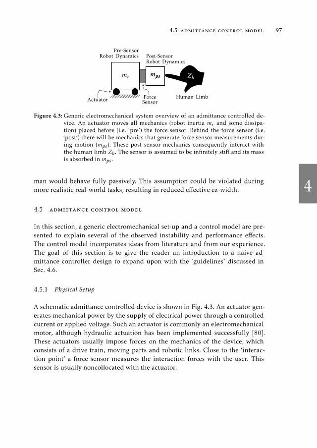
4
4.5 admittance control model 97
mr mpsmps
Pre-SensorRobot Dynamics Post-Sensor
Robot Dynamics
Human LimbForceSensorActuator
Zh
Figure 4.3: Generic electromechanical system overview of an admittance controlled de-vice. An actuator moves all mechanics (robot inertia mr and some dissipa-tion) placed before (i.e. ‘pre’) the force sensor. Behind the force sensor (i.e.‘post’) there will be mechanics that generate force sensor measurements dur-ing motion (mps). These post sensor mechanics consequently interact withthe human limb Zh. The sensor is assumed to be infinitely stiff and its massis absorbed in mps .
man would behave fully passively. This assumption could be violated during
more realistic real-world tasks, resulting in reduced effective ez-width.
4.5 admittance control model
In this section, a generic electromechanical set-up and a control model are pre-
sented to explain several of the observed instability and performance effects.
The control model incorporates ideas from literature and from our experience.
The goal of this section is to give the reader an introduction to a naive ad-
mittance controller design to expand upon with the ‘guidelines’ discussed in
Sec. 4.6.
4.5.1 Physical Setup
A schematic admittance controlled device is shown in Fig. 4.3. An actuator gen-
erates mechanical power by the supply of electrical power through a controlled
current or applied voltage. Such an actuator is commonly an electromechanical
motor, although hydraulic actuation has been implemented successfully [80].
These actuators usually impose forces on the mechanics of the device, which
consists of a drive train, moving parts and robotic links. Close to the ‘interac-
tion point’ a force sensor measures the interaction forces with the user. This
sensor is usually noncollocated with the actuator.

4
98 admittance control for physical human-robot interaction
Contro
ller
Sf
smp
Yv k
rCfb
HZOH
Hi k
r
smp
smp
Yr
Sv k
r
Sa
sZps
s
Cff
Zps
Gf
Fext
Ft
Fm
ev
ifbFc
am
v
Fdst
−vm
Fps
vd
iff igf
−Fps
Figure
4.4:E
xpan
sionoftheap
paren
trobotdynam
icsYashownin
Fig.4.1
and4.2
(note
that
itdoes
notshow
couplin
gto
thehuman
,as
isshownin
Fig.4.2).Open
circlesim
ply
summatio
n.Theblock
‘smp’im
plies
discrete
samplin
gofacontin
uoustim
esig
nal.
Theshad
edarea
isthecontro
ller,which
isim
plem
ented
insoftw
are.See
thetex
tin
Sec.4
.5.2
orthestart
ofthisch
apter
forexplan
ationoftheused
symbols.T
hetotal
transfer
functio
noftheap
paren
tad
mittan
ceYafro
mFextto
visgiven
inAppen
dix
C.

4
4.5 admittance control model 99
A force sensor has non-zero inertia, and usually a tool (for industrial appli-
cations), handle (for manual interaction) or cuff (for exoskeleton-like applica-
tions) is attached to the sensor. It will measure these post-sensor dynamics dur-
ing motion of the pre-sensor system as an impedance effect. These post-sensor
dynamics can be thought of as the known time-invariant impedance of the in-
teraction environment, and is preferably solely inertial in nature. These post-
sensor dynamics do not include the user’s dynamics. We therefore deem the
user’s impedance to be the unknown impedance of the environment, Zh. Instead
of the force sensor, the post-sensor dynamics interact with a human limb or
another object in the environment. The consequential interaction force is mea-
sured by the force sensor. The admittance controller will, due to these forces,
attempt to respond like the virtual dynamics.
4.5.2 Admittance Control Diagram
The stand-alone apparent dynamics Ya from Fig. 4.2 is shown in extended and
expanded form in Fig. 4.4, omitting the interconnection with the user (Zh). The
admittance causality is observed when noting the external force (Fext) as the
input, tracking the signal to the motion (velocity) of the system (v) as the out-
put. The complete transfer function from force Fext to motion v, describing this
system’s apparent dynamics, is given in Appendix C.
The total control diagram is comprised of several subsystems that will be dis-
cussed in the following paragraphs. Dependence on Laplace variable s is mostly
omitted for readability.
Forces on the system:
Externally applied force (Fext) by the human and his/her passive dynamics, and
forces from the post-sensor dynamics (Fps) act on this system. They are mea-
sured by a force sensor with limited bandwidth, possible filtering, or observer
dynamics (Sf ).
From measured force to desired velocity:
The signal is consequently sampled (smp) to be processed by the digital con-
troller. The measured forces (Fm) pass through the virtual dynamics (Yv), which
calculates the desired dynamical behavior. A transmission ratio (kr ) increases
the reference velocity of the virtual dynamics to the desired robot motor velocity

4
100 admittance control for physical human-robot interaction
(vd ). This velocity, which is not necessarily a state from the virtual admittance,
see section 4.6.5, is the reference signal for the velocity controller to track.
Control and actuation:
The velocity controller outputs a desired electrical current to be imposed on
the actuators by the current controller. The velocity controller consists of a feed-
forward (Cff) and feedback controller (Cfb). The feedback controller is commonly
of the PI type: Cfb = kp + ki/s. Additional force amplification (Gf) allows for
apparent reduction in robot inertia and damping/friction effects.
All reference current values from the force-amplification, feed-forward and
feedback control (igf+iff+ifb) are presented to the closed-loop current controller
(Hi ). The output value is held constant during a sample time Ts using a zero
order hold (ZOH). We assume the current controller to have high bandwidth
(commonly > 2 kHz for industrial current controllers), and some processing de-
lay that adds to the sampling-and-processing delays from the ZOH.
The controlled current generates a motor control force (Fc) that is amplified
by the gearing ratio kr . This control force acts on the passive robot dynamics
(Yr ). External forces and disturbance forces (Fdst), such as static friction and
obstructions also act on the robot and actuator.
Resulting motion and impedance effects:
The robot’s resulting motion is due to the sum of these forces. This motion is
measured by a velocity sensor or observer (Sv), and an acceleration sensor or
observer (Sa). The former is used in the closed loop velocity control. The latter
is used in compensation strategies (see Sec. 4.6.3) through Zps. Any post-sensor
dynamics (Zps, the known environment impedance), i.e. a tool or cuff, generates
impedance reaction forces Fps on the device’s force sensor and adds to the robot
dynamics directly through the forward path to Yr .
4.5.3 Control Model
We are interested in a simple model that can explain instability when in con-
tact with stiff environments. We call this model the baseline model, with which
we can compare performance of possible improvements. It constitutes a naive
admittance controller with feedback control only and virtual dynamics as in
Fig. 4.1. The robot constitutes a rigid body mass with some dissipation, and is

4
4.5 admittance control model 101
mr mps mh
Fc
v Fext
kh
bhbr
ForceSensor
Figure 4.5: Schematic view of a rigid robot. An external force Fext and a controller forcefrom an actuator Fc are applied to the robot inertia mr combined with thepost-sensor inertiamps , both resulting in some robot velocity v. Some energy-losses during robot motion are modeled as viscous damping br . The robot canbe rigidly connected to a human with inertiamh, stiffness kh and damping bh,shown by the gray dotted outline.
10−2 10−1 100 101 102−100−80−60−40−20
0
Admittance
[dB]
10−2 10−1 100 101 102−180−90
0
90
180
Frequency [Hz]
Angle
[] Yv Ya
πYa Yr
(a)
0 30 60 90 120 1500
1000
2000
3000
4000
5000
bh [Ns/m]
k h[N
/m]
mh = 0 kg
mh = 2 kg
mh = 4 kg
(b)
Figure 4.6: Behavior and performance of a typical admittance controlled system. (a) Bodeplot of the uncoupled system: apparent dynamics Ya approaches virtual dy-namics Yv for low frequencies, but the constant difference is due to sensorinertia mps . Passive system πYa has controller gains such that they conformto (4.7) and (4.8). This passive system performs poorly, very similar to therobot dynamics Yr instead of the virtual dynamics Yv . (b) The ez-width of Yacoupled to a second order impedance is larger for higher human limb inertiamh. The region of stable interaction is indicated by the arrow markings.

4
102 admittance control for physical human-robot interaction
Table 4.1: Baseline system dynamical parameters
Parameter Value
mv 2 kg
kr 1
mr 10 kg
mps 2 kg
br 5 Ns/m
kp 100 Ns/m
ki 2000 N/m
shown in Fig. 4.5. The apparent dynamics of this baseline system is denoted by
Ya. This robot can be in contact with a human that applies force Fext , which can
be from human impedance (shown in dotted gray in Fig. 4.5).
This baseline model is derived from the elaborate model in Fig. 4.4. We as-
sume ideal sensors, such that (Sf = Sv = 1), no acceleration sensing (Sa = 0), no
feed-forward control (Gf = Cff = 0), assume post-sensor impedance Zps = mpss,
and set mr = m′r +mmk2r and br = b′r + bmk
2r to add the effects of reflected in-
ertia (mmk2r ) and damping (bmk
2r ) from the motor to those of the robot inertia
(m′r ) and damping (b′r ). The used parameter values are presented in Table 4.1.
The controller attempts to make a 10 kg inertia robot with damping feel like a
pure 2 kg inertia, which gives an inertia reduction factor of five and removes
damping effects.
The equation ofmotion of the system in Fig. 4.5, omitting the human impedance,
absorbing any external force (either from human impedance or extraneous force)
into Fext(t) is given by:
(mr +mps)v(t) + brv(t) = Fext(t) + Fc(t) + krFdst(t), (4.2)
with mr the pre-sensor robot inertia and mps the post-sensor robot inertia, v(t)
the real robot velocity, br the viscous effects in the drive train, kr the trans-
mission ratio of the drive train, Fext(t) the external force applied by the user
(directly felt by the robot actuators), Fc(t) the force applied by the controller
through actuators and transmission, and Fdst(t) disturbance forces acting on
4
4.5 admittance control model 103
the robot on the actuator side. Equation (4.2) is rewritten in the Laplace-domain
(omitting dependency on s for readability) by
(mrs+ br)v = Fext −mpsvs+ Fc + krFdst . (4.3)
The controller equations for this baseline model for virtual dynamics of inertial
form (virtual inertia mv) are given by
Yv =1
mvs(4.4)
vd = krYv(Fext −mpsvs) (4.5)
Fc = krkps+ ki
s(vd − krv). (4.6)
with kp and ki the proportional and integral controller gains respectively. Equa-
tion 4.4 gives the transfer function of the virtual dynamics. Equation (4.5) shows
that the reference velocity is calculated from the measured interaction force,
namely external force Fext and the post-sensor inertial effects −mpsvs. Equa-
tion (4.6) shows a typical PI velocity controller that generates a controller force
based on the velocity error ev = vd − krv.
Uncoupled stability:
For positive choices for all parameters, the apparent dynamics created by (4.3)
to (4.6) has three poles: one of zero from the purely inertial virtual dynamics Yv ,
and two stable (possibly complex) poles from the PI-feedback controller. There-
fore, the robot is stable when in free air, when it is not held by the human.
In Fig. 4.6a is shown that the baseline apparent admittance Ya is stable, and
partially approaches the virtual dynamics Yv . For low frequencies there is a con-
stant difference in admittance modulus, which is an inertia offset due the post
sensor inertiamps. The naive admittance controller can therefore not remove any
post-sensor inertia (see Sec. 4.6.3 how to achieve this). At high frequencies the
apparent dynamics Ya drop back to the robot dynamics Yr , introducing excess
phase lag in the frequency range of the transition.

4
104 admittance control for physical human-robot interaction
Passivity of the uncoupled apparent dynamics:
Passivity of this robot is guaranteed if and only if
mv > 0
mv ≥Kp
Kp + brmr ≈mr (4.7)
−brKi ≥ 0, (4.8)
with Kp = kpk2r , and Ki = kik
2r . Equation (4.8) tells us we have to sacrifice low fre-
quency performance for passivity by setting ki = 0 (it cannot be made negative,
since that would violate the uncoupled stability requirement). This is under-
standable from the fact that the integral controller adds extra phase lag for low
frequencies onto the already marginally passive virtual inertia behavior. There-
fore any amount of extra phase lag makes the apparent admittance active. At the
passivity limit given by (4.7), which demands to have the controller introduced
pole in Ya to be of higher frequency than the introduced zero we are left with a
passive equivalent system with the same inertia as the robot itself (see Fig. 4.6a,
system πYa). Therefore, passive inertia reduction is not possible with admittance
control with a pure virtual inertia and solely using feedback control. Having
high transmission ratio (i.e. kr ≫ 1) makes it more difficult for such a system to
be passive, according to (4.7). The passivity criterion tells us to use little inte-
gral gain, and use low transmission ratio. This conflicts with good disturbance
rejection and performance.
Coupled stability:
The uncoupled baseline system with parameters described in Table 4.1 is not
passive and will have finite ez-width, when coupled to a passive environment,
as is shown in Fig. 4.6b.
All the stability boundaries in Fig. 4.6b have in common that they pass through
the origin, for any human limb inertia. This shows that admittance controlled
systems would never be stable for interaction with pure springs, or pure spring-
mass combinations. This is something that is not observed in practice, because
all realistic environments have some form of energy dissipation. The upward
slope of all curves through the origin shows that adding limb damping yields a
decent ‘stiffness margin’ and stable interaction.

4
4.5 admittance control model 105
10−2 10−1 100 101 102−80−60−40−20
0
20
Admittance
[dB]
10−2 10−1 100 101 102−180−90
0
90
180
Frequency [Hz]
Phase[]
Yv Ya Yr
(a) Accommodation Control
10−2 10−1 100 101 102−100−80−60−40−20
0
10−2 10−1 100 101 102−180−90
0
90
180
Frequency [Hz]
(b) Stiffness Control
Figure 4.7: Admittance control apparent dynamics Ya for uncoupled (a) passive ac-commodation control (bv = 80 Ns/m), (b) passive stiffness control (kv =1000 N/m). Both figures share the same legend. The low frequency mismatchin (b) is due to the integral velocity gain ki that acts like a spring in series withvirtual spring kv . In both figures the phase of Ya stays within ±90, whichshows passivity.
4.5.4 Virtual Damping and Stiffness Behavior
Naive admittance controllers can more straightforwardly render pure virtual
damping (i.e. accommodation) and pure stiffness effects passively with decent
performance. This is illustrated in Fig. 4.7a and Fig. 4.7b. For low frequencies
the apparent admittance approaches the virtual admittance well for both ac-
commodation and stiffness control. Above the feedback controller bandwidth,
the apparent admittance becomes inertial in nature due to the robot’s intrinsic
dynamics.
If in (4.4) the virtual dynamics are replaced by Yv = 1bv
(i.e. accommodation
form), the passivity conditions become
bv ≥ 0
mrKi ≤ (Kp + br)(Kp + bv).

4
106 admittance control for physical human-robot interaction
This shows again that Ki should be kept low, the robot inertia has to be low and
that either the virtual damping, robot damping or proportional gain has to be
high to have passive accommodation control.
If in (4.4) the virtual dynamics are replaced by Yv = skv
(i.e. stiffness form),
the relevant passivity condition is trivial with kv ≥ 0, when assuming positive
values for all other parameters. The apparent stiffness kapp of the device is
kapp =(
lims→0
(Yas
))−1=
(
1
kv+
1
Ki
)−1,
or two springs (the integral/position gain and the virtual stiffness) in series, as
can be seen in Fig. 4.7b. The apparent stiffness differs slightly from the virtual
stiffness due to finite integral controller gain ki .
4.5.5 Virtual Element Combinations
For combinations of mass-spring-damper elements in the virtual dynamics, the
passivity conditions become combinations of the conditions presented in the
previous sections. This leads to upper and lower limits of robot and controller
parameters that become difficult to interpret as design-guidelines in some cases.
The effective behavior of these passivity conditions, and what they effectively
teach us, is shown in Table 4.2. Note that the mass-damper combination is also
discussed in more detail in Sec. 4.6.4.
As a rule of thumb it can be stated that if virtual mass is used, the condition
in (4.7) is invariant to addition of other elements. Also, the conditions for a
spring-damper combination add directly (therefore reducing the passivity of a
pure spring), but the mass-spring combination acquires an extra addition to the
passivity condition.
Table 4.2 also gives a coupled stability robustness ranking from 1 (the best) to
7 (the worst) showing for a fixed set of controller and robot parameters, which
virtual admittance makes the robot ‘most’ passive.
Note that the virtual mass-spring-damper case is the only combination that
also has a non-trivial uncoupled stability requirement related to an upper limit
on ki . All other parameter combinations achieve uncoupled stability due to pos-
itive parameters. The generic mass-spring-damper passivity, and stability, con-
ditions are derived and shown in more detail in Appendix C.
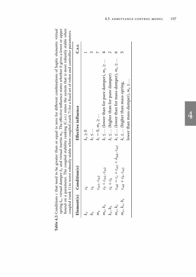
4
4.5 admittance control model 107
Tab
le4.2:C
onditionscthat
needto
begreater
than
oreq
ual
tozero
fordifferen
tcombinationsofhap
ticelem
ents:virtual
springk v,virtual
dam
per
b van
dvirtual
inertiamv.Theeff
ectiveinfluen
cestates
whether
itgives
alower
orupper
boundonaparam
eter.Thecoupledstab
ilityranking(C
.s.r.)states
thesystem
that
ismost
robustly
stab
lewhen
coupled(ran
k1)to
worstrobustly
stab
lewhen
coupled(ran
k7)forafixed
setofrobotan
dcontroller
param
eters.
Elemen
t(s)
Condition(s)
Effective
influen
ceC.s.r.
k vc k
k v≥0
1
b vc b
k i≤...
3
mv
c m1,c m
2k i=
0,m
v≥...
7
mv,b v
c b+c m
1,c m
2k i≤...(lower
than
forpure
dam
per),m
v≥...
4
k v,b v
c k+c b
k i≤...(higher
than
forpure
dam
per)
2
mv,k v
c mk=
c s+c m
1+δmk,c m
2k i≤...(lower
than
formass-dam
per),m
v≥...
6
mv,k v,b v
c mk+c b,c m
2k i≤...(higher
than
mass-sp
ring,
5
lower
than
mass-dam
per),m
v≥...
4
108 admittance control for physical human-robot interaction
4.6 guidelines for minimal inertia
In section 4.5.4 it was shown that pure damping and stiffness are readily ren-
dered passively by the robot. Therefore, we focus on the challenge of rendering
low system inertia. We expand the naive model from Sec. 4.5.3 to incorporate
and analyze additions to the control diagram that are shown in Fig. 4.4 and
were discussed in Sec. 4.5.2. We use the passivity criterion for the uncoupled
system, the ez-width of the system coupled to a passive second order system,
disturbance rejection and admittance tracking performance (i.e. how well the
apparent admittance matches the virtual admittance) to draw conclusions about
the feasibility of certain design choices. We will always compare a change in de-
sign or model to the ‘baseline’ controller from Sec. 4.5.3, and attempt the same
inertia reduction of a factor five from 10 kg to 2 kg.
From this analysis follows a set of guidelines that is presented here in random
order. The derivation of the apparent dynamical behavior, the uncoupled stabil-
ity conditions and positive real conditions for all the guidelines are shown in
Appendix C.
4.6.1 Guideline 1: Use Feed-Forward Control
If the robot controller can be used in torque (or current) control mode it is ben-
eficial to use feed-forward control. Feed-forward control can be applied in the
form of force gain (Gf > 0) and inertia and damping compensation (impedance
Cff = µffs+ βff). The passivity condition in (4.7) and (4.8) change due to the ad-
dition of feed-forward control to
mv ≥(Kp + βffk
2r )mr − (Kp + br)µffk
2r
(Gfkr + 1)(Kp + br)(4.9)
0 ≤ (βffk2r − br)Ki . (4.10)
By setting βffk2r ≥ br in (4.10), it is possible to use integral gain for good low
frequency approach of the apparent dynamics to the virtual dynamics. The feed-
forward inertia parameter µff effectively removes inertia from the robot, such
that there is less inertia to reduce by the feedback controller. This can be seen
in the numerator of (4.9) where feed-forward inertia µff is subtracted from the
robot inertiamr . The inertia-increasing effect of βff on the right hand side of (4.9)
can be counteracted by using Gf > 0.

4
4.6 guidelines for minimal inertia 109
10−2 10−1 100 101 102−80−60−40−20
0
20
Admittance
[dB]
10−2 10−1 100 101 102−180
−90
0
90
180
Frequency [Hz]
Phase[]
Yv Ya Ya Yr
Figure 4.8: Comparing the use of feed-forward control (Ya) with the baseline system Ya.It can be seen that high frequency approach of the virtual dynamics is goodfor Ya. Furthermore, the phase lag of Ya stays within passivity bounds, asopposed to Ya. Used parameter values: Gf = 5, µff = 10 kg and βff = 2 Ns/m.
For high transmission ratios, the passivity condition in (4.9) reduces to
µff ≥kp + βff
kp + bmmm.
This shows that only with feed-forward, high transmission actually helps in
achieving some passive low virtual inertia.
The use of feed-forward increases both the ez-width and improves the ad-
mittance tracking performance for high frequencies above the velocity controller
bandwidth. As is shown in Fig. 4.8, the admittance can be made passive (the ez-
width becomes infinite), while approaching the virtual admittance much better

4
110 admittance control for physical human-robot interaction
10−2 10−1 100 101 102−80−60−40−20
0
20Admittance
[dB]
10−2 10−1 100 101 102−180−90
0
90
180
Frequency [Hz]
Phase[] Yv Ya
Ya Yr
(a)
0 30 60 90 120 1500
1000
2000
3000
4000
5000
bh [Ns/m]
k h[N
/m]
mh = 0 kg
mh = 2 kg
mh = 4 kg
(b)
Figure 4.9: Influence of low-pass filtering the measured force on system performanceand interaction stability. (a) This bode plot shows a systemwith force filtering(Ya) and the baseline system Ya. The used filter is of first order with high timeconstant 0.05 s to show an extreme effect on phase-lag and consequently onez-width. It can be seen that high frequency approach of the virtual dynamicsis poor for Ya. Furthermore, the phase-lag of Ya is bigger than for Ya, resultingin a system much more unstable when in contact with a human limb. (b) Theez-width of Ya, compared to baseline (dashed lines). Due to force filtering theez-width is reduced. The region of stable interaction is indicated by the arrowmarkings.
at high frequencies than the baseline system Ya could. The apparent inertia for
high frequencies is given by
mapp =(
lims→∞
(sYa))−1
=mps +mr
µffmv
k2r +Gfkr + 1.
Without any feed-forward (i.e. Gf = 0 or µff = 0) the high frequency inertia
would always fall back to the total robot inertia mps + mr . The use of feed-
forward control passively reduces this inertia, but it cannot become lower than
mps.
4
4.6 guidelines for minimal inertia 111
4.6.2 Guideline 2: Avoid Force Filtering
It is tempting to low-pass filter force sensor measurements to reduce effects of
noise or aliasing that cause random motion of the robot. This should be avoided
if the virtual admittance is purely inertial (i.e. Yv = 1/mvs). Consider a force
sensor bandwidth limitation given by
Sf (s) = B−1n (s),
with Bn(s) a Butterworth polynomial of order n. For all orders n > 0 we add
extra poles and nπ/2 rad phase-lag to the virtual admittance Yv . This extra
phase lag directly conflicts with the relative-order constraint from the frequency
domain passivity criterion (see Sec. 4.4.2). A single pole low pass filter with time
constant τf would change the passivity condition of (4.7), only if ki = 0 to:
mv ≥mr
Kp
Kp + br+Kpτf . (4.11)
Setting ki and then picking mv on the passivity bounds would not lead to any
decrease in inertia. Adding a low pass filter with τf > 0 makes this effect even
worse, requiring an increase in virtual (and therefore apparent) inertia for the
system to be passive.
Filtering will therefore reduce ez-width (see Fig. 4.9b for an extreme case of
low-pass filtering) and limit high frequency apparent admittance performance
(see Fig. 4.9a). This is not problematic for n = 1 with accommodation control,
or n = 2 for stiffness control, which will both effectively become admittance
control due to the extra pole(s) of the filter (see Appendix C).
If filtering is inevitable, e.g. for anti-aliasing, then the filter bandwidth should
be as high as possible and the filter order as low as possible.
4.6.3 Guideline 3: Compensate Post-Sensor Inertia
Post-sensor dynamical effects are not reduced ormasked by the basic admittance
controller (Sec. 4.5.3), or by feed-forward control (Sec. 4.6.1). The post-sensor
inertial effects can be compensated in the low-frequency range by performing

4
112 admittance control for physical human-robot interaction
10−2 10−1 100 101 102−80−60−40−20
0
20Admittance
[dB]
10−2 10−1 100 101 102−180−90
0
90
180
Frequency [Hz]
Phase[]
Yv Ya Ya Yr
(a)
0 30 60 90 120 1500
1000
2000
3000
4000
5000
bh [Ns/m]
k h[N
/m]
mh = 0 kg
mh = 2 kg
mh = 4 kg
(b)
Figure 4.10: Influence of post-sensor compensation on system performance and interac-tion stability. (a) This bode plot shows a system with post-sensor compensa-tion (Ya) and the baseline system Ya. The used amount of post-sensor inertiacompensation was µc = 2 kg, the same amount as the post-sensor inertia,with low-pass filter τc = 0.1 s. The compensation improves low-frequencytracking, but generates phase lag. (b) Due to the added phase lag, the ez-width of Ya (solid lines) is lower than that of Ya (dashed lines). Post-sensorinertia compensation therefore reduces ez-width. The region of stable inter-action is indicated by the arrow markings.
post-sensor dynamics compensation (in impedance form) with a compensation
inertia µc, and low pass filter time constant τc:
ZpsSa =µc
τcs+ 1.
This improves the performance, because indeed we achieve the following appar-
ent inertial behavior at low frequencies:
Ya,low−freq ≈1
slims→0
(sYr)
=1
s(mv +mps −µc)
If µc = mps the post sensor dynamics are completely compensated, as shown in
Fig. 4.10a.

4
4.6 guidelines for minimal inertia 113
This method, however, reduces ez-width (see Fig. 4.10b). The passivity condi-
tion in (4.7) changes to (assuming τc = 0)
mv ≥Kp
Kp + br(mr + µc),
where µc effectively increased the lower bound on the value of mv .
In accordance with with Aguirre-Ollinger et al. [119, 13] this method can also
be used to effectively give the robot negative inertia. This will reduce the inertia
of the object or human limb attached to the robot. For this to work, τc > 0 (or
even higher order filters) and some limb damping bh > 0 is required.
4.6.4 Guideline 4: Use Some Virtual Damping
Virtual admittance of inertial form can in most applications be changed to a
combination of inertia and a small amount of damping
Yv =1
mvs+ bv.
The small amount of damping (bv) is hardly felt by the user, but adds useful
phase lead at lower frequencies that can lead to passivity and increased ez-
width, if the phase lead is near the excessive phase lag. Therefore, added virtual
damping is successful when the velocity controller bandwidth is low or has long
delays.
The passivity conditions in (4.8) changes, when adding some virtual damping,
to
Ki ≤ bv(Kp + bv)(Kp + br)
brmv + bvmr.
Passivity condition in (4.7) is left unaltered, i.e. adding some virtual damping
will not allow for lower mv . A third new passivity condition is the rather trivial
one bvK2i ≥ 0. Since integral gain can be increased, virtual damping allows for
better low frequency tracking (see Fig. 4.11a at the low frequencies).
Fig. 4.11b shows that ez-width becomes larger when adding some virtual
damping. A minor penalty for using damping is the dissipative nature, imped-
ing motion.

4
114 admittance control for physical human-robot interaction
10−2 10−1 100 101 102−80−60−40−20
0
20Admittance
[dB]
10−2 10−1 100 101 102−180−90
0
90
180
Frequency [Hz]
Phase[]
Yv Ya Ya Yr
(a)
0 30 60 90 120 1500
1000
2000
3000
4000
5000
bh [Ns/m]
k h[N
/m]
mh = 0 kg
mh = 2 kg
mh = 4 kg
(b)
Figure 4.11: Influence of adding virtual damping on system performance and interac-tion stability. (a) This bode plot shows a system with some virtual damping(Ya) and our baseline system Ya. The added damping has a value of bv = 2Ns/m. (b) The virtual damping reduces some phase lag. The ez-width of Ya(solid lines) is larger than that of Ya (dashed lines). Using a small amountof damping therefore increases ez-width. The region of stable interaction isindicated by the arrow markings.
4.6.5 Guideline 5: Modify the Velocity Reference
It is common that industrial robots with ‘black box’ PI velocity control (or equiv-
alently PD position control) are retrofitted with an admittance controller. In that
case, adding feed-forward (guideline 1) is not possible, and some other way has
to be found to get better admittance tracking and good ez-width.
It is possible to change the virtual admittance and add some form of accelera-
tion feed-forward with gain ka
Yv = (ska + 1)Y ′v ,
with Y ′v some intended virtual dynamical behavior. This creates phase some lead,
and better high frequency tracking of the originally intended virtual admittance
Y ′v .
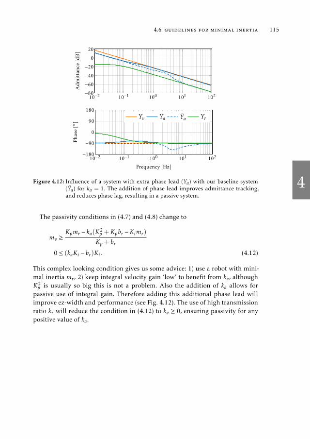
4
4.6 guidelines for minimal inertia 115
10−2 10−1 100 101 102−80−60−40−20
0
20
Admittance
[dB]
10−2 10−1 100 101 102−180
−90
0
90
180
Frequency [Hz]
Phase[]
Yv Ya Ya Yr
Figure 4.12: Influence of a system with extra phase lead (Ya) with our baseline system(Ya) for ka = 1. The addition of phase lead improves admittance tracking,and reduces phase lag, resulting in a passive system.
The passivity conditions in (4.7) and (4.8) change to
mv ≥Kpmr − ka(K2
p +Kpbr −Kimr)
Kp + br
0 ≤ (kaKi − br)Ki . (4.12)
This complex looking condition gives us some advice: 1) use a robot with mini-
mal inertia mr , 2) keep integral velocity gain ‘low’ to benefit from ka, although
K2p is usually so big this is not a problem. Also the addition of ka allows for
passive use of integral gain. Therefore adding this additional phase lead will
improve ez-width and performance (see Fig. 4.12). The use of high transmission
ratio kr will reduce the condition in (4.12) to ka ≥ 0, ensuring passivity for any
positive value of ka.

4
116 admittance control for physical human-robot interaction
4.6.6 Guideline 6: Increase Velocity Loop Bandwidth
Many passivity conditions in the aforementioned guidelines demand low kp and
low ki of the velocity controller. Nevertheless, high bandwidth control actually
improves ez-width drastically. This seemingly contradicting statement comes
from the fact that high bandwidth pushes the excessive phase lag to high fre-
quencies, becoming only an issue for higher human stiffness values. Therefore
increasing kp and ki could have beneficial effect on ez-width, while fully neglect-
ing the passivity requirement. Furthermore, higher kp and ki values ensure more
disturbance rejection at the motor side, which suppresses unwanted friction and
parasitic dynamics.
Add differential velocity control:
An additional method to increase the velocity control bandwidth is to use a PID
velocity (PDD2 position) controller [142]. The feedback controller is augmented
with differential gain kd and low pass filter time constant τd , and it takes on the
form
Cfb = kp +kis+
kds
τds+ 1.
To be a proper and implementable transfer function, differentiation is band-
limited by the low pass filter. Unfortunately, the passivity condition from (4.8)
remains unaltered. The passivity condition from (4.7) becomes:
mv ≥Kpmr + brKiτ
2d − brKd
Kp + br,
with Kd = kdk2r . This shows that the virtual inertia parameter has to be increased
if there is non-zero Ki and non-zero τd . We also obtain a new condition, very
similar to (4.7), which exists only if τd , 0. It states that still no passive inertia
reduction can be achieved
mv ≥mr
Kpτd +Kd
(Kp + br)τd +Kd≈mr .
Band-limited differential control action has little effect on the passivity condi-
tions, and it can not make the system passive with Ki , 0 and τd , 0.

4
4.6 guidelines for minimal inertia 117
10−2 10−1 100 101 102−80−60−40−20
0
20
Admittance
[dB]
10−2 10−1 100 101 102−180−90
0
90
180
Frequency [Hz]
Phase[]
Yv Ya Ya Yr
(a)
0 30 60 90 120 1500
1000
2000
3000
4000
5000
bh [Ns/m]
k h[N
/m]
mh = 0 kg
mh = 2 kg
mh = 4 kg
(b)
Figure 4.13: Influence of differential velocity control on system performance and inter-action stability. (a) Bode plot to compare a system with band limited differ-ential control (Ya) with our baseline system Ya. The parameters are kd = 25Ns2/m (i.e. kg) and τd = 0.1 s. Differential control reduces phase lag andimproves admittance tracking for high frequencies. (b) Due to the reducedphase lag, the ez-width of Yr (solid lines) is much larger than that of Ya(dashed lines). Adding differential control to the velocity controller there-fore increases ez-width. The region of stable interaction is indicated by thearrow markings.
Adding a band limited differential velocity controller assists in achieving bet-
ter high frequency approach of the virtual admittance, as is shown in Fig. 4.13a.
Adding differential gain also increases ez-width drastically, as is shown in Fig. 4.13b.
This behavior is due to the introduced zero in the transfer function due to the
differentiation, and now we can choose the location of the new pole that was
introduced by the low pass filter.
Reduce time delays:
Another method to achieve higher velocity bandwidth in practical setups is to
reduce any additional phase lag due to DA conversion (ZOH) or current con-
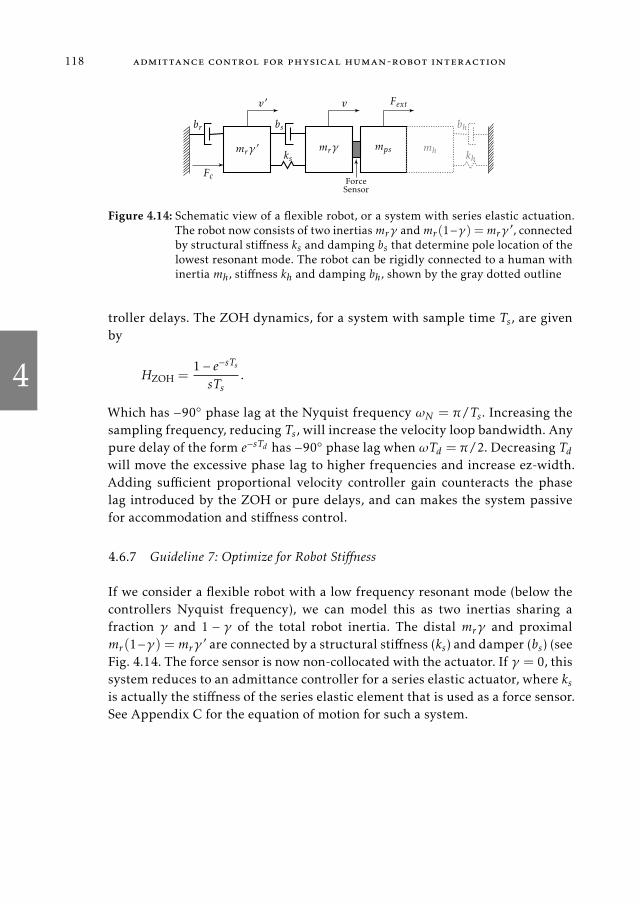
4
118 admittance control for physical human-robot interaction
mrγ′ mrγ mps mh
Fc
v′ v Fext
kh
bhbr
ks
bs
ForceSensor
Figure 4.14: Schematic view of a flexible robot, or a system with series elastic actuation.The robot now consists of two inertiasmrγ andmr (1−γ) =mrγ
′ , connectedby structural stiffness ks and damping bs that determine pole location of thelowest resonant mode. The robot can be rigidly connected to a human withinertia mh, stiffness kh and damping bh, shown by the gray dotted outline
troller delays. The ZOH dynamics, for a system with sample time Ts, are given
by
HZOH =1− e−sTs
sTs.
Which has −90 phase lag at the Nyquist frequency ωN = π/Ts. Increasing the
sampling frequency, reducing Ts, will increase the velocity loop bandwidth. Any
pure delay of the form e−sTd has −90 phase lag when ωTd = π/2. Decreasing Tdwill move the excessive phase lag to higher frequencies and increase ez-width.
Adding sufficient proportional velocity controller gain counteracts the phase
lag introduced by the ZOH or pure delays, and can makes the system passive
for accommodation and stiffness control.
4.6.7 Guideline 7: Optimize for Robot Stiffness
If we consider a flexible robot with a low frequency resonant mode (below the
controllers Nyquist frequency), we can model this as two inertias sharing a
fraction γ and 1 − γ of the total robot inertia. The distal mrγ and proximal
mr(1−γ) =mrγ′ are connected by a structural stiffness (ks) and damper (bs) (see
Fig. 4.14. The force sensor is now non-collocated with the actuator. If γ = 0, this
system reduces to an admittance controller for a series elastic actuator, where ksis actually the stiffness of the series elastic element that is used as a force sensor.
See Appendix C for the equation of motion for such a system.

4
4.6 guidelines for minimal inertia 119
10−2 10−1 100 101 102−80−60−40−20
0
20
Admittance
[dB]
10−2 10−1 100 101 102−180−90
0
90
180
Frequency [Hz]
Phase[]
Yv Ya Ya Yr
(a)
0 30 60 90 120 1500
1000
2000
3000
4000
5000
bh [Ns/m]
k h[N
/m]
mh = 0 kg
mh = 2 kg
mh = 4 kg
(b)
Figure 4.15: The influence of having a system with finite internal stiffness on systemperformance and interaction stability (a) This bode plot shows a systemwithfinite stiffness (Ya) and our baseline system Ya. The parameters are γ = 0.5,ks = 1000 N/m and bs = 100 N/m. Finite internal stiffness generates morephase lag. (b) Due to the added phase lag, the ez-width of Yr (solid lines)is lower than that of Yr (dashed lines). Finite internal stiffness of the robottherefore reduces ez-width. The region of stable interaction is indicated bythe arrow markings.
According to Colgate [143] the inertia cannot be passively reduced to any in-
ertia smaller than mrγ . Except for the condition γ ∈ [0,1], the found passivity
conditions are too complex to draw straightforward conclusions.
The performance with a high-frequency mode is acceptable (see Fig. 4.15a).
The ez-width is sensitive to γ , bs and ks. The ez-width gets smaller when low-
ering internal stiffness, lowering internal damping and increasing γ > 0, as is
shown in Fig. 4.15b. This hints at the fact that series elastic actuation, with low
γ , where the force sensor is the spring, should be well doable for admittance
controlled system.
4.6.8 Summarizing Remarks
The guidelines to achieve minimal apparent inertia of an admittance controlled
robot are summarized in Table 4.3, showing the main motivation why it helps
to follow them.

4
120 admittance control for physical human-robot interaction
Table 4.3: Summary of the seven guidelines presented in Sec. 4.5.3, together with themain motivation.
No Guideline Motivation
1 use feed-forward control effectively lowers the robot inertia to be re-duced by the admittance controller
2 avoid force filtering introduces excessive phase-lag ontomarginally passive virtual inertia model
3 compensate post-sensor inertia reduces the apparent inertia but signifi-cantly reduces coupled stability margins
4 use some virtual damping allows for better low-frequency tracking ofadmittance
5 modify the velocity reference non-physical phase-lead can give bettertracking of pure inertial model and in-creases coupled stability margins
6 increase velocity loop bandwidth pushes the excessive phase lag to higherfrequencies, which requires higher environ-ment stiffness to destabilize the coupledsystem
7 optimize for robot stiffness internal resonant modes introduce phaselag between force sensor measurement andvelocity measurement
4.7 discussion
Naive haptic admittance controllers that use only feedback control achieve pas-
sivity with good approach of the intended dynamics, when rendering pure vir-
tual stiffness or pure damping. Such controllers have difficulty rendering pure
inertia lower than the original device inertia. This is inconvenient, since the ad-
mittance control paradigm is commonly used to attempt inertia reduction of
bulky devices. The analyses in this chapter, our experience and reports in liter-
ature show that attempted inertia reduction leads to coupled instability. With a
feedback-only velocity controller, admittance controllers become unstable when
the device is firmly held by humans (e.g. for cooperative industrial tasks or hap-
tic displays) or when it is attached to limbs (e.g. for rehabilitation devices). How-
ever, completely avoiding feedback control is infeasible, since it is required to
suppress unwanted disturbances from external forces and friction forces.

4
4.7 discussion 121
The guidelines presented in this work propose several solutions to this cou-
pled instability problem when rendering virtual inertia lower than the device
inertia. The goal of these guidelines is to simultaneously 1) achieve a better
approach of the apparent dynamics to the intended virtual dynamics, and 2)
ensure robust coupled stability in the sense of passivity. The guidelines give a
qualitative description of how to design key parameters of the mechanical sys-
tem and control system. These were derived from the fact that the design has
to be close to passivity, but also approach the intended dynamics properly with
sufficient disturbance rejection. We did not discuss proper controller design (i.e.
choices for tuning feedback gains). Any objective in terms of robustness or opti-
mality could be used for determining feed-back controller gains, as long as these
are within uncoupled stability bounds, and interaction stability bounds given in
this work. The ez-width or passivity bounds should be used as optimization con-
straints during such controller design.
Using the presented framework for designing admittance controlled systems
has several limitations. We derived most of the guidelines from an idealized
stiff and single-DOF robot. In multi-DOF robots, energetic coupling between
non-linear degrees of freedom could result in instability effects absent in sin-
gle DOF analyses. A dynamical model with distributed mechanical compliance
might be more useful in practical cases. However, the analysis for a system with
a single resonant mode leads to qualitatively non-informative and complicated
conditions for passivity, uncoupled stability and interaction stability. For a dis-
tributed flexible model this would be even more so. Nevertheless, while the con-
ditions might seem complicated, they could be incorporated in design software.
In practice, velocity measurements required for velocity control can be per-
formed by tachometers (EMF based), or gyroscopes. The more common alter-
native of numerical differentiation of joint position encoder signals with high
spatial resolution leads to quantized and noisy estimates of joint velocity. Such
a noisy estimate result in a noisy or grindy feel when interacting with the robot.
Low-pass filtering this quantization noise results in unwanted resonance in the
PI velocity controller’s feedback loop and jeopardizes passivity. Therefore, es-
timation methods that use optimal integration of joint position measurements,
joint acceleration estimations and a model of the device could give a joint veloc-
ity estimation with low phase lag and a high signal to noise ratio.
However, measuring estimating the robot accelerations, also required for guide-
lines 3 and 6, can be difficult in practice. We have added first order low-pass fil-
ters to indicate limited sensor bandwidth observed in practice. Accelerometers

4
122 admittance control for physical human-robot interaction
output noisy signals, resulting in a noisy feel of the device during interaction.
Other acceleration estimation methods, such as double numerical differentia-
tion of joint-encoder measurements yield heavily quantized and noisy estima-
tions as well. Possible state observer models together with optimal sensory inte-
gration could aid in obtaining an optimal estimation of the acceleration. Note
that guidelines 1 and 5 do not need acceleration measurements. These use the
accelerations from the virtual dynamics, which are derived from the force mea-
surements.
The analyses in this work focused mostly on the influence of isolated param-
eter changes. Coupled parameter changes, for example by using feed-forward
control and a low-pass filter on the force concurrently, were not discussed. Ap-
plying two guidelines, or changing two system variables could show unexpected
interaction.
We briefly discussed the influence of ZOH and time-delay effects on passivity
properties. Using discrete time sub-models for the feedback controller, virtual
dynamics and possible state estimators might give slightly different and more
realistic passivity conditions. Nevertheless, since haptic devices usually use fast
sampling frequencies above 1000 Hz, we assume that the found guidelines are
valid.
The post-sensor effects analyzed were assumed to be purely inertial. In prac-
tice we notice that post-sensor backlash and flexibility leads to unwanted limit-
cycles. Whether this behavior is to be expected from the apparent dynamics in
combination with coupled post-sensor dynamics, or exhibit a different form of
instability, has to be further analyzed.
5
5SP I S : SWITCHING DAMPING ADMITTANCE CONTROL FOR
STABLE INTERACT ION WITH INERT IA REDUCT ION
Arvid Q.L. Keemink, Niek W.M. Beckers and Herman van der Kooij
The stability was illusory.
— Liu Cixin, The Three-Body Problem, 2006
Abstract–Attempting to reduce inertia with admittance control can result in
an unstable system during human-robot interaction. In this work we show
the origin of this active behavior. We present a simple stabilization method
that activates a virtual damper only if the virtual energy stored in the vir-
tualmodel becomes higher than the real energy exchanged between the robot
and the human. This damper dissipates excess energy built up in the virtual
model dynamics, which ensures stable interaction between humans and ad-
mittance controlled robots with inertia reduction. Model simulations on a
linear one degree-of-freedom system and a validation of the method on a
non-linear two degree-of-freedom haptic setup show the simplicity and ap-
plicability of the method.
list of used symbols and abbreviations
Symbol Explanation
∅ the empty set or empty subsystem
0 0-junction, common effort (bondgraph)
1 1-junction, common flow (bondgraph)
a passivity polynomial coefficient
Ab(t) time-varying system transition matrix
b(ξ) generalized damping coefficient dependent on system state
b SPIS damper value
Bv dissipative subsystem of intended (virtual) dynamics
cr subscript: between controller and robot mechanics
123

5
124 switching damping admittance control for stable interaction
C feedback controller
diss subscript: relating to dissipation
e tracking error
ext subscript: relating to external influence
E exchanged energy between two systems
E0 energy initially stored in dynamical system
f force vector
fs discrete time sample frequency
F generalized force
subscript: relating to force
h subscript: relating to the human
hr subscript: between human and robot mechanics
hv subscript: between human and virtual dynamics
H energy stored in a system as potential and kinetic energy
I interface through with (virtual) power flows
J(q) manipulator Jacobian
k generalized mechanical stiffness, gain or sample instant
K controller gain matrix
m, M generalized mechanical inertia
subscript: measured
M inertia tensor
MSe modulated source of effort (bondgraph)
MSf modulated source of flow (bondgraph)
P mechanical power
q(t) vector of joint angles
r subscript: relating to the robot mechanics
R, R+ set of real numbers, set of positive real numbers
S switching surface (decision boundary)
t, τ time
T controller sample time
v generalized velocity
subscript: relating to the virtual model
v(t) velocity vector

5
switching damping admittance control for stable interaction 125
vc subscript: between virtual dynamics and controller
vol subscript: relating to voluntarily applied fore
x generalized position
x(t) linear position vector
X set of achievable states
Y (virtual) dynamical system with admittance causality
z discrete time domain variable of the z-transform
z(t) vector of expanded system state
z∞ attractor
Z (virtual) dynamical system with impedance causality
Z set of achievable expanded states
Z+ set of the positive integers (incl. 0)
ZOH zero-order-hold dynamical system
α, β, γ admittance controller parameterization parameters
Γ energy dissipated internally in a dynamical system
δ amount of spring penetration
δe(t) difference between stored energy Hv and transmitted energy Ehr (t)
ǫ initial distance between inertial mass and springs in Fig. 5.3
η(t) vector of generalized Coriolis and centrifugal forces
ξ(t) vector of system state
ω angular frequency
Ω subspace of Z, split by S
Abbrev. Explanation
DOF degree of freedom
PD proportional-derivative
PI proportional-integral
PRC positive real condition
SP strict passivity
SPIS strict passivity inspired stability
UUB uniform upper bound

5
126 switching damping admittance control for stable interaction
5.1 introduction
Safety and dependability are key to successful integration of robots into human
environments or to use them as wearable power augmentation devices. Haptic
interaction control methods, like admittance control, are used to achieve this
goal bymaking a robotic device behave like a safe mechanical impedance during
physical human-robot interaction [68, 87].
During admittance control, the robot movement is controlled to follow a mo-
tion reference that is derived from how a virtual dynamical model with admit-
tance causality responds to the applied forces from a human operator. In this
way, the robot impedance felt by the operator imitates the impedance of this
virtual model. A basic version of the control diagram is shown and explained
in Fig. 5.1. Admittance control allows strong and heavy robots to be moved by
the human operator with ease. Human power augmentation is hence achieved
by masking of the drive train friction, reduction of apparent inertia and cancel-
lation of gravity of the the robot itself and lifted tools and objects [94]. Such a
controller is relevant for, for example, having a robot lift unknown heavy loads
while the human is supposed to feel a constant low inertia.
Attempting to reduce inertia with admittance control with a feedback con-
troller only, by giving the virtual model an inertia value lower than that of
the real system, can result in system instability when the robot is in contact
with the operator or a stiff environment. This instability during contact, or cou-
pling, can be explained as energetically non-passive (i.e. active) behavior of the
robot [92, 63, 94, 72, 88, 144] (see also Chapter 4, Sec. 4.4).
In this work we show two different viewpoints on causes of active behavior
in admittance control, which have been overlooked in literature. We show that
recently developed methods in literature to achieve time-domain passivity for
admittance control with either time-delays [145] or inertia reduction [146] fun-
damentally do not solve admittance control’s apparent activity problem during
inertia reduction. We present a switching damper controller to dissipate at least
the actively generated amount energy and achieve stable interaction of an ad-
mittance controlled robot in contact with stiff environments while achieving
high inertia reduction factors. The introduced damping does, however, reduce
interaction performance.

5
5.1 introduction 127
Yv C YrF vd e Fc Ft v
−
Figure 5.1: Basic admittance controlled system. An external force F is measured and‘applied’ on a virtual admittance model Yv which results in desired velocityvd . A PI velocity controller C tries to enforce the desired velocity on robot dy-namics Yr by applying control force Fc . The resulting, real velocity is given byv. Note that the system would be theoretically equivalent with a PD positioncontroller.
5.1.1 Passivity and Passivity Enforcement
Consider a continuous-timemechanical dynamical systemwith a power-conjugated
force and velocity input-output pair (F(t),v(t)). The energy exchanged at time
t between the coupled operator and this dynamical system is given by
E(t) =
∫ t
0F(τ)v(τ)dτ+ E0. (5.1)
Here E0 is the energy initially stored in the system at t = 0. Positive energy
(E(t) > E0) implies net energy transferred to the system, whereas negative en-
ergy (E(t) < E0) implies net energy transferred to the operator.
For a system to be energetically passive, or just ‘passive’, the following neces-
sary and sufficient time-domain passivity condition is required
E(t) ≥ E0 ∀t. (5.2)
This condition implies that the system never returns more energy to the user
than the user ever provided to the system.
Passive systems, and interconnections of passive systems, are stable [92]. In-
voluntary human forces generated by intrinsic limb impedance and reflexes
have been found to behave mostly passively [99], although not always [141].
Nevertheless, from everyday experience we know that human interaction with
passive objects (e.g. grasping, lifting, pulling or dragging of non-actuated ob-
jects in the real world) always leads to stable interaction. Therefore, ensuring
passive behavior of a robotic system during physical interaction with a passive

5
128 switching damping admittance control for stable interaction
human operator guarantees interaction stability by putting the responsibility of
stable interaction on the human’s controller.
Several authors have presentedmethods to enforce passivity on haptic devices
in the frequency domain according to the positive real condition (PRC) [92, 68].
Time-domain passivity (i.e. upholding (5.2)) was enforced on dynamical simu-
lations or open loop impedance causality type haptic devices by Hannaford and
Ryu et al. by damping away excess energy at the man-machine port [147, 148].
For dynamical simulations with integration methods that would otherwise re-
sult in instability, passivity has been enforced by calculating model states back
from the Hamiltonian, enforcing energy conservation as a constraint [149].
For admittance control in the form as shown in Fig. 5.1 the PRC dictates
that passive inertia reduction is, in fact, impossible. If a high amount of con-
stant damping in the virtual dynamics is used [144] (see Chapter 4), a small
amount of passive inertia reduction can be approached for low interaction fre-
quencies. However, adding this required amount (or more) of constant damp-
ing does not allow for more passive reduction of the apparent virtual inertia.
Furthermore, it results in an over-damped system that is sluggish and is unnec-
essarily damped when free-floating. A possible solution to this problem is to
use computed torque (feed-forward) control [144] (see Chapter 4) in the inner
motion control loop. Such control requires proper models of the robotic sys-
tem, which might be complicated, expensive or intractable for multi degree of
freedom (DOF) real systems. Furthermore, the PRC gives usually a black-box
condition for passivity, not stating the origin of the active behavior.
Only recently sampled time domain passivity enforcement has been attempted
for admittance control [150, 146, 145]. The focus of the work of De Stefano et
al. [145] was not on inertia reduction but on compensating the active behavior
of time-delays by applying a time-delay-passivity-network. Nabeel et al. [146]
built on this idea to attempt using the same method to enforce passivity for iner-
tia reduction systems. The work of Nabeel et al. is highly ambiguous as to which
variables at which sample instants are actually required and used; their desired
velocity modification results in an algebraic loop that is not properly resolved.
Furthermore, the applied method in [150, 146] is inherently flawed, as they ne-
glect the actual origin of the active behavior, as will be discussed in this work
in detail in Sec. 5.2. Appendix D presents a counter-example to the method pre-
sented in [146] that shows that their passivity controller cannot guarantee any
kind of passive behavior during inertia reduction due to a wrong assumption
about the source(s) of the active behavior.

5
5.2 energetic behavior 129
In this work we develop a method to yield a stable interaction between an
admittance controller that attempts to reduce inertia and an environment with
knownmaximal stiffness. We do this by observing the energy exchanged through
the power port at the human-robot interface and the human-virtual model inter-
face (see Ihr and Ihv in Fig. 5.2) and by using a switching virtual damper on the
virtual model accordingly. We avoid using extra forces in the low-level velocity/-
position controller, because these are sometimes non-accessible during design
on retrofitted industrial manipulators or when using low-level controllers that
perform their own motion control.
The chapter is organized as follows: in Sec. 5.2 we discuss standard admit-
tance control and how different kinds of energy flow through different inter-
faces. In Sec. 5.3 and Sec. 5.4 we use the relevant energy observed to develop
a strict passivity inspired stability (SPIS) controller for admittance control. In
Sec. 5.5 we validate the controller stability in simulation and in a real nonlinear,
two DOF haptic setup.
5.2 energetic behavior
For an admittance controlled robot coupled to a person there are multiple real
and virtual energy flows between the human, actuators, virtual model elements
and the robot mechanics.
A bondgraph diagram [151] is a concise and insightful way to show energy
flows between dynamical elements or subsystems across different physical do-
mains. It can be used to visually and conceptually separate them from signals
that only carry information but no energy. Fig. 5.2 shows a bondgraph diagram
of the real and virtual power flows and signals used to model an admittance con-
trolled device interacting with a human. The the directed half-arrows ( or )
represent power-bonds, where the tip of the half-arrow indicates the defined di-
rection of positive physical power flow between energy sourcing, sinking or stor-
ing dynamical elements. Normal arrows (→) indicate information carrying sig-
nals between elements. In other words, a power bond resembles a bi-directional
(i.e. ) power-conjugate pair of physical effort (i.e. an across variable, such as
mechanical force or electrical voltage) and physical flow (i.e. a through variable,
such as mechanical velocity or electrical current) ‘signals’. The perpendicular
line at the and or start of the half arrow (i.e. or ) indicates the direction
of the effort. The accompanying flow has to go in the opposite direction. This
determines the causality of the connected subsystem: admittance or impedance

5
130 switching damping admittance control for stable interaction
MSe
Fm
1vd
Yv
MSf
vd
0Fc
C
1vr
Yr
0 Fh
1v Zh
MSe
Fh,vol
z −1
ZOH
=
Ihv
Icr
Ihr
Ivc
Fc(k)
Fc(t)
vr(k)
vr(t)
Figure
5.2:A
bondgrap
hdiag
ram[151]ofan
admittan
cecontro
lledrobotinteractin
gwith
ahuman
.Thebluecolorindicates
virtu
alsig
nal
andpower
flow
(timevariab
lek∈
Z+),whereas
theblack
colorindicates
mech
anical
power
flow
(timevariab
let∈
R+).Human
imped
ance
Zhan
dvoluntary
force
Fh,vol
apply
force
Fhontherobotmech
anics
Yr ,resu
ltingin
motio
nvr ,which
togeth
erexch
angephysical
power
Ehrwith
thesystem
throughpower
portI
hr .
Force
Fhissam
pled
bythesystem
asFm.Thisvirtu
alforce
Fm
isap
plied
bythemodulated
source
ofeffort
(MSe)
onvirtu
aldynam
icsYv,exch
angingvirtu
alpower
EhvthroughportI
hv.Thevelo
citysource
(MSf)
that
imposes
model
velo
cityvdan
dthecontro
ller’s(C
,an
imped
ance)
force
Fcconstitu
tevirtu
alpower
Evcthat
flowstoward
stherobotmech
anics
throughportI
vc .T
herobotmech
anics
velo
cityvran
dcontro
llerforce
Fcen
sure
theexch
ange
ofen
ergyfro
mthecontro
llerto
therobotmech
anics
(Ecr )
throughportI
crthat
addsto
thepower
that
therobot
mech
anics
exch
angewith
thehuman
(Ehr ).
Thepower
bondcro
ssinginterfaceI
crisnotaproper
power
bonddue
tothesin
gle
sample
timedelay
andzero
-ord
er-hold
(ZOH)in
thedirectio
noftheeffort
(seetheinset
with
dash
edoutlin
e).Note
that
themodel
velo
cityvdis
only
uni-d
irectionally
connected
tothemodulated
source
offlow
by
thenorm
alarro
w,constitu
tinganon-power
conjugated
connectio
nbetw
eentw
osu
bsystem
s.Alth
oughmisu
sing
proper
bondgrap
hnotatio
n,th
e0junctio
nontherig
htsid
eisused
tomeasu
retheinteractio
nforce,an
deffectiv
elystates
that
v=
vr .

5
5.2 energetic behavior 131
causality. For example, systems with admittance causality have effort-in, flow-
out causality. Such a system should have the perpendicular line at the end of
the half-arrow close to the sub-system with admittance causality (since the force
is an input, and the model velocity is the output of an admittance model). The
junctions shown by the numbers 0 and 1 indicate common effort (all connected
elements share the same effort, such as serial mechanical springs or parallel elec-
trical impedances) and common flow (all elements share the same flow, such as
a spring connected to a mass or electrical impedances in series) respectively. An
ideal modulated source of effort (e.g. an ideal variable force/voltage source) is
given by MSe, and an ideal modulated source of flow (e.g. an ideal variable
velocity/current source) is given by MSf. Passive subsystems with admittance
causality are denoted by Y , and passive subsystems with impedance causality
are denoted by Z .
We distinguish four relevant real and virtual power ports that energy passes
through, denoted by interfaces I , where interaction between sub-systems takes
place. The continuous time index is given by t, the discrete time index by k. Note
that we lump the actuator and controller into a single system and will hence-
forth talk about energetic behavior of the controller. We also assume that motor
torque is controlled with sufficiently high bandwidth such that the controller
becomes an ideal effort source [151]. These four power ports are where:
• The controller supplies real energy Ecr(t) from the controller to the robot
mechanics through Icr .
• The human operator supplies real energy Ehr(t) from the human to the
robot mechanics through Ihr .
• The human operator supplies virtual energy Ehv(k) from the human to the
virtual model through Ihv .
• The virtual model supplies virtual energy Evc(k) from the virtual model
to the controller through Ivc.
Virtual dynamics Yv are passive, and might contain an intended dissipative
subsystem Bv ⊆ Yv that functions as an energy sink. The controller C is com-
monly a passive PD-position, or PI-velocity, controller. Both the robot’s mechan-
ical dynamics Yr and the human’s limb impedance Zh are both continuous-time,
passive, immitances.
We recognize that the connection between the virtual model and the con-
troller is uni-directional, and therefore not a power-conjugated one (as is also

5
132 switching damping admittance control for stable interaction
mentioned in [152]). This is visible in Fig. 5.2, where the flow source for vdis only uni-directionally connected to the virtual model, without any reaction
force acting back on the virtual model.
5.2.1 The Admittance Controller’s Inherently Active Behavior
The active behavior of a continuous time implementation of an admittance con-
troller* is effectively stated by the restrictions on controller parameters put forth
by the PRC. Nevertheless, the PRC’s black-box input-to-output passivity analy-
sis does not explain the virtual or physical source of this active behavior for
a standard admittance controller. It only states which coefficients need to be
greater/smaller than others to achieve passive behavior. Therefore, analysis into
the source of the active behavior will prove useful in determining a method to
stabilize the coupled system.
A Time-Domain Interpretation:
Admittance controlled systems that attempt to reduce inertia can become un-
stable when in contact with stiff environments; e.g. by hitting a hard surface or
being tightly held by a human operator. A model of a similar event is shown in
Fig. 5.3. An inertial massM is at rest at position x(0) = 0 m. A constant positive
voluntary force from the human Fh,vol is applied to this mass for a duration tFseconds. This accelerates the mass towards the right; to one of the two unilat-
eral compliant elements (i.e. springs resembling e.g. a human hand) at distance
ǫ2 from the starting position x(0). This human compliance creates a repulsive
spring force Fh,s = −(x − ǫ2)kh only if x > ǫ2. A second unilateral compliance is
added on the opposite side, at a distance of ǫ1 from x(0), to constrain the range
of motion. In the limit of ǫ1 = ǫ2 = 0 the two unilateral compliant elements
form a single typical bilateral spring with stiffness kh, modeling the robot being
held by a human operator.
We define two different cases of this system that will be investigated further:
1. An admittance controlled robot: M is the robot mass mr . The admittance
controller measures both the human forces (Fh,vol and Fh,s), and applies
control force Fc to attempt to reduce this inertia to the lower value of mv .
*In this work we ignore possible extra sources of (virtual) energy that arise due to quantizationor sampling.

5
5.2 energetic behavior 133
M
x,v
Fh,vol khkh
ǫ1 ǫ2
Figure 5.3:Model of a 1D mass M colliding with unilateral human compliance kh afterpositive (pointing to the right) force Fh,vol acts for a time tF . The springsare at initial distance ǫ1 and ǫ2 from the starting position x(0) = 0 m. AftertF seconds, the force stops accelerating mass M . After moving a distance ǫ2mass M will collide with the right-most spring. Afterwards, the mass M willbounce towards the other spring and the cycle continues. The position andvelocity of the mass are given by x and v respectively. Note that if ǫ1 = ǫ2 = 0this is equivalent to a typical mass-spring system with a bilateral spring withstiffness kh.
The robot uses a PD position controller to track the reference position xd(t)
and velocity xd(t) = vd(t) coming from the virtual model:
mr x(t) = Fc(t) + Fh,s(t) + Fh,vol(t) (5.3)
mv xd(t) = Fh,s(t) + Fh,vol(t)
Fc(t) = kp(xd(t)− x(t)) + kd(vd(t)− v(t))
2. The passive intention (denoted as ‘intended’ or ‘intention’ in the text): M
is virtual mass mv , i.e. no admittance control used:
mv x(t) = Fh,s(t) + Fh,vol(t)
For both cases, their dynamical behavior is shown in Fig. 5.4. The robot mass
was mr = 1 kg, while the virtual mass was mv = 0.5 kg. The controller is a PD
position controller with gains kp = 1000 N/m and kd = 100 Ns/m. The human
compliance was modelled as a linear stiffness kh = 1000 N/m. The applied force
Fh,vol was applied for a duration of tF = 0.1 s. To achieve 1 J of energy supplied
(Ehr ) to the passive intended behavior, the force magnitude had to be 10 N. The
springs were located at a distance ǫ1 = ǫ2 = 0.2 m from the mass’ initial posi-
tion.
The intention (case 2) is passive by definition. The mass mv will accelerate,
gather momentum and energy due to the applied human force. After moving
distance ǫ2 it collides with the spring and penetrates a distance δ into the spring.
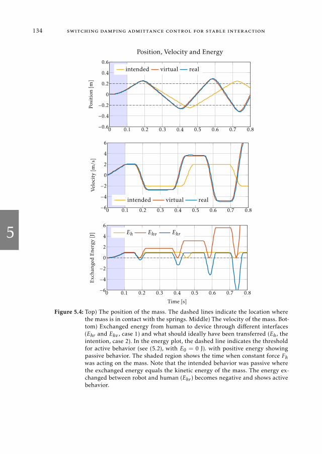
5
134 switching damping admittance control for stable interaction
0 0.1 0.2 0.3 0.4 0.5 0.6 0.7 0.8−0.6
−0.4
−0.2
0
0.2
0.4
0.6
Position[m
]
Position, Velocity and Energy
intended virtual real
0 0.1 0.2 0.3 0.4 0.5 0.6 0.7 0.8−6
−4
−2
0
2
4
6
Velocity
[m/s]
intended virtual real
0 0.1 0.2 0.3 0.4 0.5 0.6 0.7 0.8−6
−4
−2
0
2
4
6
Time [s]
Exch
anged
Energy[J] Eh Ehv Ehr
Figure 5.4: Top) The position of the mass. The dashed lines indicate the location wherethe mass is in contact with the springs. Middle) The velocity of the mass. Bot-tom) Exchanged energy from human to device through different interfaces(Ehr and Ehv , case 1) and what should ideally have been transferred (Eh, theintention, case 2). In the energy plot, the dashed line indicates the thresholdfor active behavior (see (5.2), with E0 = 0 J). with positive energy showingpassive behavior. The shaded region shows the time when constant force Fhwas acting on the mass. Note that the intended behavior was passive wherethe exchanged energy equals the kinetic energy of the mass. The energy ex-changed between robot and human (Ehr ) becomes negative and shows activebehavior.
5
5.2 energetic behavior 135
The spring will push back the mass towards the spring on the other side, result-
ing in a marginally stable bouncing cycle. The kinetic energy initially supplied
by the human’s voluntary force Fh,vol is fully converted to potential energy by
the spring kh during collision. This potential energy is in turn converted back to
kinetic energy by the spring’s repulsive force. There is no net energy gained or
lost by the interaction of these passive elements.
During admittance control with inertia reduction (case 1) the mass will accel-
erate and start to move as intended when the force Fh,vol is applied. The mass
will collide with the spring, but penetrates a distance δ′ > δ into the spring. The
spring will push the mass towards the spring on the other side. The admittance
controlled mass exits the spring with a velocity higher than its incoming velocity,
i.e. some kinetic energy is ‘created’. Consequently, it hits the other spring where
this process repeats. This results in an unstable, or growing, cycle.
The cause of this active behavior is twofold, but both causes are explained by
the accumulated phase lag of the inner motion loop in the admittance controller.
The motion controller’s output force always lags behind the motion reference
coming from the virtual model. As a consequence, the human (i.e. the spring kh)
experiences the controlled robot to have more inertia than the mv it was trying
to simulate. Therefore:
1. it will penetrate deeper into the spring, experiencing a larger repulsive
force Fh,s than was intended,
2. the ‘robot mass’ also spends more time inside the spring than was in-
tended.
Consequently, the reaction force Fh,s from the spring acts for a longer amount
of time on the virtual model than was intended. This leads to accumulation of
more virtual momentum, and therefore more virtual energy, than was intended.
This results in a higher velocity when leaving the spring than the initial velocity
at the moment of colliding with the spring.
Fig. 5.4 shows that the energy transferred between the robot and user (Ehr )
becomes negative during a collision. This implies a net energy transfer to the
human operator that is bigger than what the human operator introduced. Ev-
ery consecutive bounce this amount of energy returned to the human operator
increases in magnitude. The human (a pure spring) resupplies all that same
amount of energy back to the robot, leading to a never exceeded maximum of
approximately 1 J of kinetic energy physically stored in the robot, like in the
intended case.

5
136 switching damping admittance control for stable interaction
γ Yv C Yr
α
β
F vd e Fc Ft v−−
Figure 5.5: Admittance controlled system as shown in Fig. 5.1, but parameterized withbinary α, β and γ that have a value of either 0 or 1. Parameter α representsbackdrivability and should be 1 for a physical system. Parameter β representsthe bi-directionality of the spring-damper controller in C (i.e. a PD-positionof PI-velocity controller), i.e. if β = 1 the controller will also apply reactionforces on the virtual model. Parameter γ allows for the copying of the interac-tion force to the virtual model. A typical admittance controller has α = γ = 1and β = 0.
The virtual energy transferred between the virtual model and user (Ehv) goes
to 0 J during every collision, like in the intended case. However, after a collision
the transferred energy has increased; the excess energy resupplied to the human
operator is fed back to the virtual model with a non-trivial amount of scaling.
The energy exchanged between user and robot (Ehr ) has the correct (i.e. in-
tended) upper limit, whereas the energy exchanged between the user and vir-
tual model (Ehv) has the correct lower limit. Therefore, an inertia reduced ad-
mittance controlled robot that bounces against a stiff surface, or is held in place
by finite stiffness, will exhibit active behavior that presents itself as a growing
oscillation.
A Systems Interpretation:
Fig. 5.2 shows that there is a uni-directional connection between the virtual
model and the subsequent controller-robot dynamics. This effectively means
that the controller impedance C, as a PD position controller, acts like a uni-
directional spring-damper between the virtual model and the robot dynamics.
The robot dynamics feel the virtual model but not vice versa. Consequently we
parameterize the controller from Fig. 5.1 with several binary gains α, β and γ .
Parameter α turns on/off backdrivability. Parameter β adds a ‘physically consis-
tent’ feedback of the controller (as is shown in Fig. 5.5) to make the controller

5
5.2 energetic behavior 137
a bilateral spring-damper. Parameter γ determines whether the force on the
robot is copied onto the virtual model. With these parameters, the PRC gives
the following condition for frequency-domain passivity (see Appendix D for
the derivation):
a2ω4 + a1ω
2 + a0 ≥ 0, ∀ωa2 =mv(αmv(br + kd)−γkdmr)
a1 = br(k2dβ(αβ+ γ)− kpmv(2αβ+ γ))
a0 = βbrk2p (αβ+ γ).
For (marginal) passivity, a negative a1 can be balanced by both a positive a2and a0 for several parameter values. Although we are here not interested in
parameter values to determine the passivity boundary, this passivity condition
readily tells us three important things:
1. If α = 0 and γ = 1 then the system is never passive, since this makes a2 < 0,
which makes it active for high frequencies.
2. If β = 1 it is ‘more passive’ than if β = 0, since it makes a0 > 0. So the
uni-directional spring (β = 0) is a source of activity.
3. If γ = 0, with α = β = 1, the system would be always passive; it would be
a spring-damper interconnection between two passive systems.
Therefore, it is shown that it is the copying of the force from the human to the
virtual model (i.e. the modulated source of effort that acts as an energy source),
together with the uni-directional spring-damper from the controller that cause
active behavior. This shows why the method of Nabeel et al. [146] cannot work,
since it only attempts to make the uni-directional spring-damper element pas-
sive, neglecting the active behavior of the modulated effort source. In the work
of De Stefano et al. [145] the problem is not circumvented, but solely hidden, by
not attempting inertia reduction and performing compensation only for energy
introduced due to time-delay. It also shows that solutions developed for tele-
operation methods to do negate active effects of time-delay, such as developed
in [153], will not work on admittance control, since in those scenarios the force
is not copied from the slave side directly onto the master.

5
138 switching damping admittance control for stable interaction
5.3 stability and passivity conditions for admittance control
In this section we will revisit the passivity condition given in (5.2), and put forth
a more strict passivity condition to derive a stabilizing controller that is useful
for admittance controlled systems.
We make the notational distinction between energy exchanged through power
ports (I in Fig. 5.2) denoted as ‘E’ and energy stored in systems denoted as ‘H’.
For example, the energy stored in the virtual system has to be the difference
between the energy exchanged between the human and the virtual model (Ehv)
and the energy dissipated internally Γ(t)
Hv(t) = Ehv(t)− Γ(t).
We assume in this and the following derivations that the initial energy E0 = 0 J
and that no intended damping behavior is required (i.e. Bv = ∅).
5.3.1 Strict Passivity (SP)
Because Hv(t) is the virtual energy stored in the system as kinetic energy in
the virtual model, this energy has a definite lower bound because it cannot be
negative:
Hv(t) ≥ 0, ∀t.
If we wouldmakeHv(t) a lower bound for Ehr(t), it would follow that Ehr(t) ≥ 0,
∀t, which makes the system strictly passive at interaction port Ihr . Therefore, asufficient condition for strict passivity (SP) is
Ehr(t) ≥Hv(t) ≥ 0, ∀t. (5.4)
In this way, the typical (marginal) passivity condition in (5.2) is upheld at the
human robot interface Ihr . Relating to the results in Fig. 5.4, trying to enforce SP
amounts to forcing the ‘real’ (Ehr ) and ‘virtual’ (Ehv) energy to at least coincide.
Note that in Fig. 5.4 the virtual energy was the exchanged virtual energy Ehv(t)
instead of stored virtual energy Hv(t). However, in a damping free system these
are equivalent.

5
5.3 stability and passivity conditions for admittance control 139
The SP condition in (5.4) is useful, but more strict than the typical passivity
condition in (5.2). Because, even if Hv(t) ≥ 0, and Hv(t) ≥ Ehr(t) ≥ 0, the SP
condition would not hold but system is still passive according to (5.2).
5.3.2 Strict Passivity Inspired Stability (SPIS)
SP requires that the energy difference δe(t) = Hv(t) − Ehr(t) should go to, or
below, 0 J. This can be attempted in the following way:
• DecreasingHv(t): by damping away energy in the virtual modelHv(t)will
decrease its value towards, or below, Ehr(t). Moreover, the human might
interact with the virtual damper behavior through Ihr , resulting in forced
energy dissipation, in turn increasing Ehr(t) as preferred. Because the sates
in Yv are a function ofHv(t), this will cause a state change, such as a lower
desired velocity. This might result in reducing Ehr(t), resulting in slower
reduction of δe(t) → 0. Especially for low virtual model velocities this
becomes less effective.
The aforementioned agrees qualitatively with the analysis described in Sec. 5.2.1;
the mass motion should be damped in either the virtual model, or in the real sys-
tem†, to spend less time inside the spring to reduce the accumulation of excess
momentum and kinetic energy.
To force δe(t)→ 0 we put a damper (attached to ground) on the virtual model
Yv only when Hv(t) ≥ Ehr(t). Because the motion-control-loop has finite band-
width and possible tracking overshoot, it cannot be guaranteed that the velocity
of the robot v(t) goes to 0 as quickly as the virtual model velocity vd(t). For
high enough damping values this will force δe(t)→ 0 if Hv(t) ≥ 0, but cannot
enforce Ehr(t) ≥ Hv(t) at all times. Therefore the switching damping controller
enforces Strict Passivity Inspired Stability, or SPIS.
We will show in the next section that this method cannot be used to make
the system passive. It can, however, make it stable in the sense that it exhibits
bounded oscillatory behavior.
†Forcing an increase in Ehr (t) through the low-level controller, instead of the virtual model,might also help in making the system strictly passive. However, this will not be discussed in thiswork.

5
140 switching damping admittance control for stable interaction
5.4 linear dynamical analysis of spis
In this section we will analyse the dynamics of a linearized, ideal robot that
is admittance controlled, with SPIS enforced. The robot will be attached to a
linear spring with stiffness kh. We assume that the energy exchanged through
interfaces Ihr and Ihv can be properly determined, or determined with known
uncertainty, in a real system by measuring robot interaction force and motion
states. See Appendix D for how this energy bookkeeping is carried out.
5.4.1 System Dynamics
The system dynamics are assumed to be autonomous and linear, with state
ξ(t) ∈ X ⊆R4, given by state vector and state equation
ξ(t) =[
x(t) v(t) xd(t) vd(t)]T
ξ(t) = f (ξ) = Ab(ξ)ξ(t).
The system matrix Ab(ξ) is derived from (5.3), being
Ab(ξ) =
0 1 0 0
− kpmr− kh
mr− kdmr
kpmr
kdmr
0 0 0 1
− khmv
0 0 − b(ξ)mv
,
where
b(ξ) =
b, if Ehr(t) < Hv(ξ)
0, if Ehr(t) ≥Hv(ξ),(5.5)
with b > 0. Eq. (5.5) denotes the switching damper ‘controller’ used to enforce
SPIS.
5
5.4 linear dynamical analysis of spis 141
Augmented System Dynamics
The state vector is augmented with human-robot interaction energy Ehr(t). The
new state vector is denoted by z(t) ∈ Z ⊆R5, and it is given by
z(t) =
ξ(t)
Ehr(t)
, z(t) =
ξ(t)
Ehr(t)
=
Ab(ξ)ξ(t)
−khx(t)v(t)
.
This augmented system is autonomous with (5.5) describing a switching surface
S ⊂ Z, where
S =
z(t) | Ehr(t) = Hv(z)
,
splits Z into two regions Ω0 (where b(ξ) = 0) and Ω b (where b(ξ) = b, b > 0).
On the switching surface the damper value switches between 0 and b or vice
versa, depending on z(t).
If SP could be enforced, all trajectories would never be able to leave Ω0. We
would then demand that all trajectories only enterΩ0 through S and never exit,
i.e. we would enforce that
−∇(Hv(z)−Ehr(t)) · ξ(t) > 0.
I.e., the inner product of the inward normal of the switching surface S and the
system rate z(t) would need to be positive. This gives the condition
b(ξ)v2d (t) + khx(t)v(t)(vd(t)− v(t)) ≥ 0, ∀t,
which effectively equals
Pdiss(t)−Fh(t)(vd(t)− v(t)) ≥ 0, ∀t.
This shows again that from a time-domain perspective (see Sec. 5.2) it is the
velocity error, combined with the spring force, generating energy that leads to
non-strictly-passive behavior. This energy should henceforth be dissipated by
a virtual damper b(ξ) that dissipates with power equal to Pdiss. However, we
cannot guarantee that Pdiss(t) > Fh(t)(vd(t) − v(t)) at all times, due to possibly
small values of vd(t) that require unreasonably high values of b(ξ). It also shows
that an uniform upper bound (UUB) on the velocity error would limit the active

5
142 switching damping admittance control for stable interaction
behavior of the system, explaining the apparent success of Morbi et al. [154] to
limit the active behavior of an admittance controlled system.
Stability of SPIS
Eq. (5.5) acts like a sliding-mode-like controller to make the system converge
to a stable cycle during interactions with the pure spring environment. This
controller will make the interaction stable and cannot make it generally passive.
The initial conditions of the admittance controlled system are always such
that x(0) = xd(0), v(0) = vd(0) and E0 = Ehr(0) = g(v(0),x(0)) with g(·) some
function of the initial states. Therefore the system always starts with zero track-
ing error and starts by definition on switching surface S .If z(t) ∈ Ω b, and b was chosen in such a way that Ab(ξ) is asymptotically
stable, then by linear Lyapunov argument that system will converge to the point
z∞ =[
0 0 0 0 E0
]T∈ Ω0. Therefore, all trajectories z(t) ∈ Ω b are initially
attracted to move towards Ω0, and will hit S in finite time.
If z(t) ∈ Ω0, or on S , The dynamics Ab(ξ) with b(ξ) = 0 is unstable. There-
fore, z(t)will then not converge to z∞ and will slide on S or be ejected out ofΩ0
in finite time, through S , back into Ω b. From this moment on, the cycle repeats.
For dynamics Ab(ξ) that are stable when z(t) ∈ Ω b, but that have ‘too little’
damping, the instability when in z(t) ∈ Ω0 adds more energy to the system
than is dissipated when z(t) ∈ Ω b before hitting S again. The cycle will grow
and eventually the trajectories will not enter Ω0 anymore because Ehr becomes
more negative over time. Trajectory z(t) will then stay in stable Ω b and the
cycle will stop growing. The exchanged energy from the robot to the user will,
nevertheless, have become more negative. This cycling behavior for ‘too little’
damping is an outward converging cycle.
For ‘sufficiently high’ values of b the energy generated by the instability when
z(t) ∈Ω0 can be dissipated when z(t) ∈Ω b before hitting S . In this way, cycling
behavior ensures that the trajectories pass through both Ω0 and Ω b indefinitely.
This leads to an inward converging cycle.
The switching damper b(ξ) acts as a sliding-mode-like controller, such that
the apparent dynamics are mostly that of S . Therefore, this switching system
will show stable cycling behavior, as is intended for the discussed dynamics
shown in Fig. 5.3 and 5.4. The only necessary condition for a converging cycle
is that b is chosen such that Ab(ξ) is at least marginally stable when z(t) ∈ Ω b.
There is no straightforward method to calculate the required minimal value of

5
5.5 validation 143
b to ensure an inward converging cycle. Therefore, its value needs to be found
numerically, or it can be set to any sufficiently high value.
Response to Active Environments
The analysis in Sec. 5.4.1 holds for an autonomous system, e.g. an admittance
controlled system interacting with a passive pure spring. However, to be useful
the method should also work when in contact with an active human limb. Any
voluntary forces of the human can introduce energy into, or extract energy from,
the virtual model and robot dynamics through both interfaces Ihv and Ihr . Thisis shown by the force Fh,vol from the modulated source of effort (MSe) in Fig. 5.2.
Although the energetic behavior of an active human force is unpredictable,
we reason that using the switching damper from (5.5) results in stable interac-
tion in that case as well. If the human supplies energy (Ehr(t) > 0, Ehv(t) > 0)
both Ehr(t) and Ehv(t) will increase. If, due to unstable behavior, Ehv(t) in-
creases above Ehr(t), the switched damper starts dissipating energy (Γ(t)) until
Hv(t) = Ehv(t) − Γ(t) is smaller than Ehr(t), if possible. If Ehr(t) becomes nega-
tive (active behavior) the stored energy Hv(t) cannot become negative, but only
approach a value of 0 J; i.e. a stationary system with vd = 0 m/s. This gives the
system time to dissipate enough energy to achieve Ehr(t) > 0 before allowing
new motion. Hence, the interaction between the human limb and the unstable
system is hereby stabilized.
5.5 validation
In this section we validate the switching damper in simulation and in a two
DOF haptic setup. The simulated dynamics are those described in the analysis.
The real system, however, is not autonomous in the sense that a human operator
moves the robot and can introduce energy into the system or extract it.
5.5.1 Simulation
The numerical simulation of the admittance controller was performed inMatlab
2015b with a variable-step continuous-time dynamics solver. The model param-
eters were mr = 1 kg, mv = 0.1 kg, kd = 100 Ns/m, kp = 1000 N/m. The admit-
tance controller hence attempts an inertia reduction of a factor of 10. A damper
value b = 5 Ns/m makes Ab(ξ) strictly stable when in Ω b, for an inward con-

5
144 switching damping admittance control for stable interaction
(a)
−0.4−0.200.20.4
0.1
0.2
0.3
0.4
0.50.3
0.225
0.2
0.50.3
px [m]
py[m
]
Workspace, Max. Apparent Physical Inertia [kg]
(b)
Figure 5.6: a) The used haptic setup. b) Workspace of the used haptic setup with theworkspace boundary shown in black. During the experiment, the end-effectorwas forced to remain inside the shaded green circle. The level sets of esti-mated maximum apparent physical inertia (the inertia felt by the user) areshown for values of 0.2, 0.225, 0.3 and 0.5 kg. The maximum and minimuminertia were calculated as the maximum and minimum eigenvalue of the ma-nipulator mass matrix expressed in Cartesian coordinates. The lowest max-imum physical inertia value across the workspace is 0.185 kg, located nearcoordinate p = [0,0.25]T . The minimal physical inertia (not shown) in theused circular workspace was between 0.16–0.2 kg. The maximal physical in-ertia was around 0.4 kg. The virtual inertia was set to be 0.05 kg. Therefore,inertia reduction factors were therefore estimated to lie between 3.2 and 8.
verging cycle of the switching system. A damping value of 2.8881 Ns/m makes
Ab(ξ) marginally stable when in Ω b, for an outward converging cycle of the
switching system. The model started with initial position of x = xd = 0 m veloc-
ity v = vd = 1 m/s and initial energy Ehr(0) = Hv(0) = 0.05 J.
5.5.2 Haptic Setup
The SPIS method was also validated on a two DOF haptic setup (see Fig. 5.6a).
The setup consists of two actuated joints, which are denoted by the vector q(t) ∈R
2 (in rad). They drive a parallel kinematic chain, known as a five-bar link-
age. The links connected to the motor have a kinematic length of 153 mm. The
subsequent links connected to the end-effector have a kinematic length of 238
mm. Each joint is driven by a Faulhaber 3890-048-CR, spaced 70 mm apart.
Each motor is driven by high-bandwidth current control by a Technosoftmotion
5
5.5 validation 145
iPOS4808 BX-CAT driver over an EtherCAT bus. The motors are connected to
the links through a 1:7.3 capstan transmission. Absolute encoders at the joints
measure joint position with a resolution of 216 values per revolution. Forces
on the end-effector were measured by a ME-Systeme 6-axis K6D27 100N/2Nm
force/torque sensor, read by a GSV-1A8USB K6D amplifier connected to the
EtherCAT bus. The control software was implemented in Simulink 2016b, and
compiled for TwinCAT3 real-time target software that interfaces with the hard-
ware. The control software ran at a sample frequency of fs = 1000 Hz.
The continuous-time (time index t) dynamics and discrete-time (discrete-time
index k, sample duration T = 1/fs = 1 ms) jointspace PD position control of the
setup are given by:
Mq(q)q(t) + η(t) = τ(kT ) + JT (q)fext(t)
τ(kT ) = Kp(qd(kT )−q(kT )) +Kd(qd(kT )− q(kT )),
withMq(q) ∈R2×2 the jointspace mass matrix, q(t) and q(t) the angular acceler-
ations and velocity respectively, η(t) ∈R2 the vector of Coriolis and centrifugal
forces, τ ∈R2 the actuator torques, J(q) ∈R
2×2 the manipulator Jacobian, fext ∈R
2 the external force applied by the user, and Kp = diag[10,10] Nm/rad, Kd =
diag[0.1,0.1] Nms/rad diagonal proportional and derivative feedback gains re-
spectively.
Jointspace reference qd(t), qd(t) is determined through an inverse kinematic
mapping of an operational space reference (xd (t) and its time derivatives) to
jointspace (qd(t) and its time derivatives). The operational space motion refer-
ence comes from the discrete-time Cartesian two DOF virtual model, expressed
by semi-implicit Euler integration‡:
vd(k+ 1) = vd(k) + TM−1v [−b(k)vd(k) + fext(k)]
xd(k+ 1) = xd(k) + Tvd(k+ 1).
We assume a scalar b, isometric over the used workspace. The virtual mass ma-
trix is given by isometric Mv = diag([mv , mv ]), where mv = 0.05 kg. This gives
between a 3.2 to 8 times reduction in apparent inertia of the setup (see Fig. 5.6b).
‡Compared to the explicit (forward) Euler method, the semi-implicit Euler method is a first or-der symplectic integration method and almost conserves the energy in a dynamical system, makingit an almost passive numerical integration scheme. Leap-frog integration (i.e. velocity Verlet) is analternative symplectic integrator of second order and a has even better energy conserving properties.Nevertheless, active behavior due to the energy generated in by numerical integration is negligiblein this work.

5
146 switching damping admittance control for stable interaction
The virtual stored energy of the end-effector is calculated by
Hv(k) =1
2vTd (k)Mvvd(k).
The damper b(k) is switched from a value of 0 Ns/m to b = 20 Ns/m when
Hv(k) ≥ Ehr(k). This amount of damping was found empirically to be sufficient
for stable interaction with an admittance controller that reduces the end-point
inertia to 0.05 kg. Theoretically, it would be stable for linear stiffness up to ap-
proximately 175 N/m.
5.6 results
In this section we discuss the results from simulation and experiment.
5.6.1 Simulation Results
The results in Fig. 5.7 show the behavior described in Sec. 5.4.1. For b = 5 Ns/m,
the system is able to dissipate enough energy when in Ω b to have the cycle
converge inward. The cycle settles, while continuously switching between Ω b
and Ω0, showing oscillatory behavior of both the virtual model and the robot
dynamics. This oscillatory behavior is preferred, since the virtual dynamics and
the environment together are a mass-spring system without damping, for which
undamped oscillatory behavior is expected. For b = 2.8881 Ns/m, the system is
not able to dissipate enough energy when in Ω b to have the cycle converge in-
ward. An increasing amount of energy is transferred to the user (Ehr(t) becom-
ing more negative), until trajectories z(t) do not enter Ω0 anymore. However,
sinceΩ0 is by construction marginally stable, the system will converge to stable
cycling behavior.
5.6.2 Haptic Setup Measurement Results
The results in Fig. 5.8 compare a typical admittance controller (b = 0 Ns/m
always) and the admittance controller with the switching damper from (5.5).
Fig. 5.8a–c show how for typical admittance control the system became unstable
quickly after touching the end effector by hand with a piece of soft foam. The
system was aggressively unstable and could be touched only briefly and not
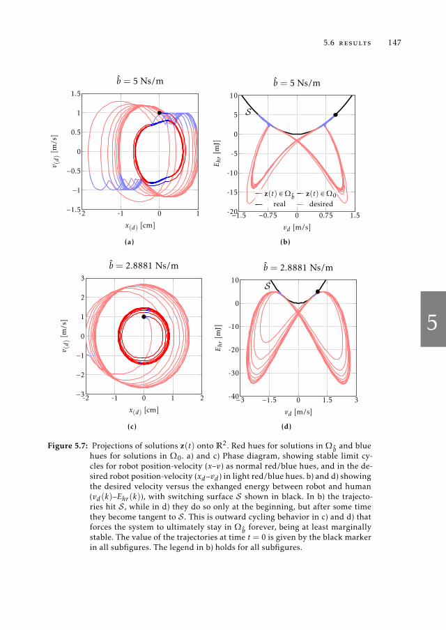
5
5.6 results 147
-2 -1 0 1−1.5
−1
−0.5
0
0.5
1
1.5
x(d) [cm]
v(d)[m
/s]
b = 5 Ns/m
(a)
−1.5 −0.75 0 0.75 1.5-20
-15
-10
-5
0
5
10
S
vd [m/s]
Ehr[m
J]
b = 5 Ns/m
z(t) ∈Ωb z(t) ∈Ω0
real desired
(b)
-2 -1 0 1 2−3
−2
−1
0
1
2
3
x(d) [cm]
v(d)[m
/s]
b = 2.8881 Ns/m
(c)
−3 −1.5 0 1.5 3-40
-30
-20
-10
0
10 S
vd [m/s]
Ehr[m
J]
b = 2.8881 Ns/m
(d)
Figure 5.7: Projections of solutions z(t) onto R2. Red hues for solutions in Ωb and blue
hues for solutions in Ω0. a) and c) Phase diagram, showing stable limit cy-cles for robot position-velocity (x–v) as normal red/blue hues, and in the de-sired robot position-velocity (xd–vd ) in light red/blue hues. b) and d) showingthe desired velocity versus the exhanged energy between robot and human(vd (k)–Ehr (k)), with switching surface S shown in black. In b) the trajecto-ries hit S , while in d) they do so only at the beginning, but after some timethey become tangent to S . This is outward cycling behavior in c) and d) thatforces the system to ultimately stay in Ωb forever, being at least marginallystable. The value of the trajectories at time t = 0 is given by the black markerin all subfigures. The legend in b) holds for all subfigures.

5
148 switching damping admittance control for stable interaction
80
81
82
83
−0.6
−0.4
−0.2 0
0.2
0.4
t[s]
Vel. [m/s]
vd,x
vd,y(a)
80
81
82
83
−1 0 1
t[s]
Force [N]
Fh,x
Fh,y(b)
80
81
82
83
−0.01 0
0.01
t[s]
Energy [J]
Ehr
Hv(c)
114
115
116
117
−0.6
−0.4
−0.2 0
0.2
0.4
t[s]
Vel. [m/s]
vd,x
vd,y(d)
114
115
116
117
−1 0 1
t[s]
Force [N]
Fh,x
Fh,y(e)
114
115
116
117
−0.01 0
0.01
t[s]
Energy [J]
Ehr
Hv(f)
Figure
5.8:M
easurem
entdata.
Thead
mittan
cecontro
llerred
uced
inertia
from
realinertia
intheran
ge0.16–0.3
kgto
acon-
stant0.05kg.a–
c)Typical
admittan
cecontro
l.Thesetu
pwas
touch
edlig
htly
byauser
byhan
dthroughapiece
of
softfoam
durin
gtheshad
edtim
einterv
als.Thesetu
pbecam
eag
gressiv
elyunstab
leim
med
iately.Thisisrefl
ectedin
thequick
build
-upofnegativ
eEhr .d–f)Admittan
cecontro
lwith
SPIS.Thesetu
pcould
now
bemoved
byhold-
ingthehan
dle
directly.
Thesetu
pwas
moved
durin
gtheshad
edtim
einterv
al.Note
that
inf)theen
ergydoes
not
beco
meincreasin
gly
negativ
e,an
dthesto
reden
ergyHvan
dexch
anged
energ
yEhrare
forced
tobenearly
equal
when
above0J,showingan
almost
strictlypassiv
ebeh
avior.
5
5.7 discussion 149
by a human hand directly. While touching the manipulator end-effector, some
energy is introduced into the system to make it move. However, more energy
is afterwards returned to the user, as is shown by Ehr in Fig. 5.8c. The energy
exchanged between the setup and the human becomes more negative over time,
showing the active behavior introduced by the instability.
Fig. 5.8d–f show measurements performed on the same setup, but with SPIS
(b = 20 Ns/m). In this case, the setup could be properly held by the operator
without it becoming aggressively unstable. Force measurements for this exper-
iment show higher force peak magnitude in Fig. 5.8e, compared to Fig. 5.8b.
This happened because the setup could be properly held and moved by a user.
Also, the switching damper introduces some mechanical impedance that in-
duces forces on the force sensor due to the human’s impedance. The stored en-
ergyHv and exchanged energy Ehr in Fig. 5.8f are similar in value when both are
positive. Also, the real exchanged energy (Ehr ) does not become more negative
over time (as happens in Fig. 5.8c), showing stable and almost passive behavior.
5.7 discussion
The proposed SPIS admittance controller was shown to be able to stabilize in-
teraction of an admittance controlled system with inertia reduction being in
contact with a stiff environments in simulation, and during real physical human-
machine interaction.
5.7.1 Limitations and Practicalities
It was not yet shown that this method works in general for virtual dynamics that
have compliant elements and intended internal dissipation. It is expected, how-
ever, that the method is as applicable in those cases as well, since the amount
of virtual potential energy is known. Furthermore, admittance control can sim-
ulate compliance passively [144] (see Chapter 4, Sec. 4.5.4).
The amount of required damping b can be set a priori to achieve a cycle that
converges neither inward nor outward. Analytical stability proofs that comple-
ment the qualitative reasoning in Sec. 5.4.1 might shed some light on this issue
and give conditions on the minimally required value of b. However, in practice
any high value that ensures a stable system is sufficient (as is shown in the re-
sults in Fig. 5.7 and Fig. 5.8), although increasingly higher values of damping

5
150 switching damping admittance control for stable interaction
result in more aggressive dissipation and higher impedance forces on the setup
due to stuttering.
This leads to another apparent problem of the implementation of the current
method that uses solely feedback control. The choice to use a low virtual in-
ertia comes from the demand for low interaction impedance. Active behavior
generated by this inertia reduction (i.e. impedance reduction) requires added
impedance from the switching damper to stay stable. As a consequence there
still significant device impedance. Possibly feed-forward contributions to the
controller could reduce the required impedance to stay stable (see Chapter 4,
Sec. 4.8).
Three practical approaches to determining the proper amount for b are as fol-
lows: 1) adding a constant amount of damping to a typical admittance controller
until the system shows no interaction instability across all practical operator
stiffness values. The system will then be impeding and dissipative due to this
damper. The SPIS method will then effectively switch off this damper when it
is not required to dissipate energy for stabilization. 2) Adaptively increasing b
when the exchanged energy between human and robot is negative when device
velocity is zero. 3) If the force sensor at the interaction port is made compliant,
its stiffness becomes the upper bound for the all environment stiffness values
the device will ever interact with. This allows to calculate and set a fixed value
for b when the device dynamics are known. This has as a drawback, however,
that the point of interaction with the device becomes compliant, something that
might not be preferred.
5.7.2 Comparison with Literature
In this work it was shown that the controller proposed by Nabeel et al. [146]
cannot guarantee passivity at the human-robot interface when inertia reduction
is attempted (see Appendix D for a counter-example to their method). Their
method, similar to the one used by De Stefano et al. [145] is only sufficient
to handle energy generated due to time-delays, but cannot remove the exact
amount of energy to make an admittance controller with inertia reduction pas-
sive. The main reason why their method cannot be applied is that the system
is not solely active due to the unilateral connection between virtual model and
the controller, but also due to the copying of the measured force that acts on the
robot mechanics onto the virtual dynamics. Any proper controller that makes
5
5.7 discussion 151
the system passive should therefore act on both the virtual model as on the real
robot mechanics.
5.7.3 Comparison with Impedance Control
Time domain passivity enforcement of open-loop impedance controlled haptic
devices that have to display virtual environments has been reported in litera-
ture. If a bondgraph (similar to 5.2) would be drawn of an impedance controlled
system, it would be apparent that the system connections are physically consis-
tent (albeit that possible inertia, damping and stiffness reduction through open
loop impedance control requires negative element values). Because impedance
controlled devices respond with a reaction force to motion, its active behavior
is in their case solely due to time discretization of the virtual model dynam-
ics. Therefore passive sampling methods [149] and adding damping forces at
the motor side [147] are sufficient to counteract active behavior and make the
system passive.
For admittance controlled systems, however, we have noticed the intercon-
nection between subsystems is non-physical on two levels: copying of the inter-
action force and the uni-directionality of the controller. On top of that, minor
energy-sources due to sampling, delays and integration methods also introduce
more energy into the system in both the virtual model and by the controller onto
the robot mechanics.
5.7.4 Future Work
The current SPIS method makes the system neither passive, nor strictly passive,
because damping takes place in the virtual model alone. Adding extra damping
in the low-level position control might assist in increasing Ehr in (5.2) and (5.4),
possibly making the robot passive or strictly passive. However, this requires
access to low level motion controllers, something that might not available. Fur-
thermore, it is not trivial to determine how to divide the dissipation amount be-
tween the two dampers while being in contact with an unknown environment.
Therefore we will investigate this in future work.

5
152 switching damping admittance control for stable interaction
5.8 conclusion
In this work we presented a method to enforce stability of an admittance con-
trolled system that attempts to reduce inertia when in contact with stiff environ-
ments. The method relies on keeping track of the exchanged energy of the hu-
man with the robot and the energy stored in the virtual dynamics. If the energy
stored in the virtual dynamics is higher than the exchanged energy, a constant
damper dissipates energy from the virtual model. This allows for stable interac-
tion behavior through a simple method that does not require modifications to a
low level motion controller.

5
5.8 conclusion 153


Part III
SHARED CONTROL :DAMPING FORCES AROUND
REACHING TARGETS


6
6US ING POS IT ION DEPENDENT DAMPING FORCES
AROUND REACHING TARGETS FOR TRANSPORT ING
HEAVY OB JECTS : A F ITTS ’ LAW APPROACH
Arvid Q.L. Keemink, Rik I.K. Fierkens, Joan Lobo-Prat, Jack S.F. Schorsch, David A.
Abbink, Jeroen B.J. Smeets and Arno H.A. Stienen
It is easier to resist at the beginning than at the end.
— Leonardo da Vinci
Abstract–Passive assistive devices that compensate gravity can reduce human
effort during transportation of heavy objects. The additional reduction of in-
ertial forces, which are still present during deceleration when using gravity
compensation, could further increase movement performance in terms of ac-
curacy and duration. This study investigated whether position dependent
damping forces (PDD) around targets could assist during planar reaching
movements. The PDD damping coefficient value increased linearly from 0
Ns/m to 200 Ns/m over 18 cm (long PDD) or 9 cm (short PDD). Movement
performance of reaching with both PDDs was compared to damping free
baseline conditions and to constant damping (40 Ns/m). Using a Fitts’-like
experimental design 18 subjects performed a series of reaching movements
with index of difficulty: 3.5, 4.5 and 5.5 bits, and distances 18, 23 and 28
cm for all conditions. Results show that PDD reduced (compared to baseline
and constant damping) movement times by more than 30% and reduced the
number of target reentries, i.e. increasing reaching accuracy, by a factor of 4.
Results were inconclusive about whether the long or short PDD conditions
achieved better task performance. However, mean human acceleration forces
were higher for the short PDD, hinting atmarginally fastermovements. Over-
all, PDD is a useful haptic force to get humans to decrease their reaching
movement times while increasing their targeting accuracy.
This chapter was published as: A.Q.L. Keemink, R.I.K. Fierkens, J. Lobo-Prat, J.S.F. Schorsch,D.A. Abbink, J.B.J. Smeets and A.H.A. Stienen, “Using position dependent damping forces aroundreaching targets for transporting heavy objects: A Fitts’ law approach”, IEEE/RAS-EMBS Interna-tional Conference on Biomedical Robotics and Biomechatronics (BioRob), 2016. The first two au-thors contributed equally to this work.
157

6
158 using position dependent damping forces around reaching targets
list of used symbols and abbreviations
Symbol Explanation
a Fitts’ law intercept
b Fitts’ law reciprocal data transmission rate
D reaching distance
ID index of difficulty
MT movement time
p probability
rm Fitts’ law regression coefficient, taking all values per subject
rm Fitts’ law regression coefficient, taking only mean metric value per
subject
W target width or diameter
α statistical significance level
χ2 Friedman ANOVA test statistic with χ2 distribution
Abbrev. Explanation
B1 baseline experiment block; no damping movement
B2 baseline experiment block; final repetition of baseline condition
C1 condition 1 experiment block; constant damping coefficient of 40
Ns/m
C2 condition 2 experiment block; damping coefficient increasing over
18 cm from 0 to 200 Ns/m at the target
C3 condition 3 experiment block; damping coefficient increasing over 9
cm from 0 to 200 Ns/m at the target
F familiarization block
nDOF Friedman ANOVA test statistic degrees of freedom
PDD position dependent damping
W1,W2,W3 washout experiment blocks

6
6.1 introduction 159
6.1 introduction
Understanding physical interaction between humans and mechatronic devices
can be useful in the field of teleoperation, rehabilitation and power augmenta-
tion robotics. Shaping the interface dynamics and reflected forces when inter-
acting with (virtual) objects (i.e. haptics) allows for task performance optimiza-
tion. For example, gravity and inertia compensation can reduce physical effort
during lifting tasks, and haptic shared control can increase situational aware-
ness and task accuracy in remote transportation tasks [155]. Although interac-
tive robotic manipulators are extremely versatile in their applications and func-
tionality, such as the admittance controlled devices used in industry [156], they
pose an inherent safety risk during physical interaction with users. Passive sys-
tems, comprised of mechanically passive elements such as springs and damper-
s/brakes, could be preferred over active systems for specific tasks. Advantages
of passive systems include the reduced design complexity, increased inherent
safety (although energy can be stored in springs), reduced (maintenance) costs,
and increased mobility due to reduced weight and power demands. Examples
of passive systems are the mobile Lockheed Fortis [157] in industry, the station-
ary rehabilitation exoskeleton Dampace [28], and the ankle-foot exoskeleton by
Collins et al. [158].
Compared to active systems, the types of forces that can be generated with
purely passive systems are limited. Such limitation is partially overcome in
Cobot systems by scaling and changing passive dynamical properties accord-
ingly through continuous variable transformers [104, 66].
We propose a system inspired by the Cobot systems, but for reaching-like
tasks. Controlled damping forces around a reaching target (position dependent
damping, or PDD) will be used to optimize a person’s motion during human-
machine cooperative tasks of picking and placing of heavy objects. The term
‘controlled’ implies the use of a physical passive element of which its dissipative
properties are varied, e.g. by controlled disk brakes or varying a moment arm of
a dash-pot damper. The term ‘optimize’ implies that movements become faster
and easier to perform with higher accuracy and subjective likability. A poten-
tial industrial application of PDD would be assisting cooperative transportation
of heavy objects with a passive gravity compensation mechanism to a target lo-
cation by a human operator, where the target is determined by range finding
sensors. The PDD could then be used for faster and more accurate placement of
heavy objects by the human operator.

6
160 using position dependent damping forces around reaching targets
In this study we investigated how PDD changes the human’s reaching strategy
and performance in terms of reaching time, accuracy and applied force during
Fitts-like [159, 160] reaching tasks. Additionally, we evaluated whether Fitts’
law still holds during reaching with PDD. We used the PDD to help them brake
the reaching movement and improve reaching accuracy and therefore move-
ment performance.
6.2 background
Modeling human reaching is challenging due to nonlinear arm and muscle dy-
namics, high muscle redundancy and the required optimal integration of both
visual and proprioceptive information [161, 162]. Fitts proposed a simple lin-
ear relationship that models speed-accuracy trade-offs in rapid, aimed two-way
tapping [159] or one-way reaching [160] movements:
MT = a+ b · ID. (6.1)
This relationship describes the movement time (MT ) as a function of Index of
Difficulty (ID) and two empirical coefficients a and b, which are dependent on
environment properties. In [163] it is proposed to use the Shannon formulation
of the ID (in bits) as a function of reaching distance D and target size/diameter
W around that target:
ID = log2
(D
W+ 1
)
, (6.2)
which we will use in the remainder of this work.
Few studies investigated validity of Fitts’ law in dissipative environments.
In [164, 165] it was shown that moving underwater (a dissipative, but highly
inertial environment) can be described by Fitts’ law with minor modification.
Further studies [166, 167, 168] investigated the influence of constant friction
and damping on the movement times. They found that for small masses (below
2 kg) a friction force could reduce reaching times and increase accuracy in a
Fitts type targeting tasks.
In contrast to the aforementioned studies, we are interested in moving heavy
masses (12.5 kg, motivated by the industrial application) and in position depen-
dent damping forces around the reaching target, instead of constant damping or
friction forces.

6
6.3 methods 161
F B1 C# W1 C# W2 C# W3 B2
18 63 63 63 6363 18 18 18
387Figure 6.1: Trial blocks presented to the subject. Numbers above the blocks indicate num-
ber of trial repetitions. F: Familiarization; B1: Baseline1 condition (nondamp-ing); C1, C2 and C3: Damping condition 1–3 with either constant dampingor specific PDD; W1, W2 and W3: Washout phase 1–3 without damping; B2:Baseline2 condition (nondamping). Dashed outlines indicate these blocks arenot used for data analysis.
6.3 methods
6.3.1 Experimental Conditions
In this experiment we compared three damping conditions (C1, C2 and C3)
where subjects performed reaching tasks with different damping forces. These
conditions were also compared to two baseline conditions (B1 and B2) with-
out any damping forces during the reaching task. These baselines were used to
observe possible overall performance improvements during the complete exper-
iment.
During reaching tasks in conditions C1, C2 and C3, subjects would feel differ-
ent viscous damping forces Fd (in N):
Fd = −b(x)v, (6.3)
where b(x) (in Ns/m) is a damping coefficient (d.c.), possibly dependent on po-
sition x (in m) for PDD, v (in m/s) is the instantaneous velocity of the moved
manipulandum. The minus sign in (6.3) shows that this force opposes the mo-
tion and makes the dynamical system passive. The d.c. was dependent on condi-
tions as shown in Fig. 6.2. Baselines B1 and B2 had zero d.c. Condition C1 had
constant d.c. of 40 Ns/m. Conditions C2 and C3 had 0 Ns/m d.c. at the start of
the movement, ramping up linearly to 200 Ns/m over a distance of 18 cm (C2)
or 9 cm (C3) from the target at D. The d.c. was never lower than 0 Ns/m, nor
higher than 200 Ns/m. Familiarization (F) and washouts (W1, W2 and W3) had
zero d.c.
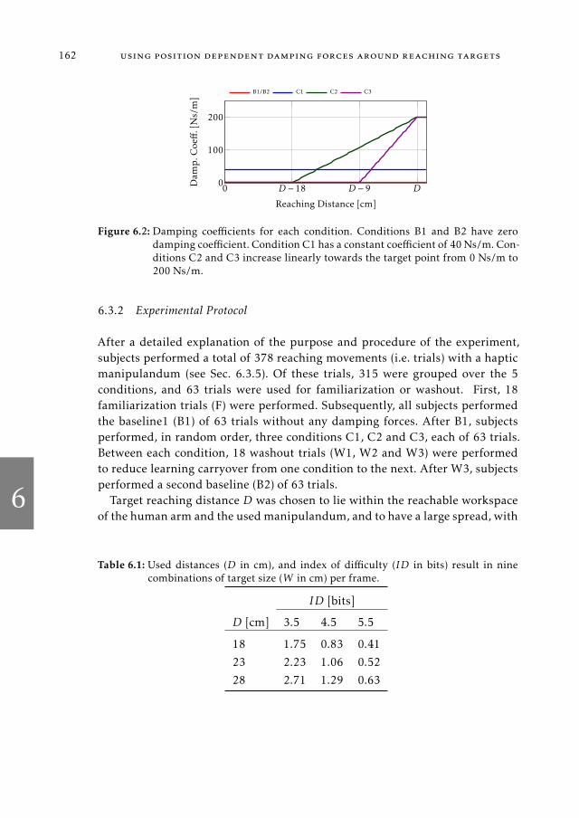
6
162 using position dependent damping forces around reaching targets
0 D − 18 D − 9 D0
100
200
Reaching Distance [cm]Dam
p.Coeff
.[N
s/m]
B1/B2 C1 C2 C3
Figure 6.2: Damping coefficients for each condition. Conditions B1 and B2 have zerodamping coefficient. Condition C1 has a constant coefficient of 40 Ns/m. Con-ditions C2 and C3 increase linearly towards the target point from 0 Ns/m to200 Ns/m.
6.3.2 Experimental Protocol
After a detailed explanation of the purpose and procedure of the experiment,
subjects performed a total of 378 reaching movements (i.e. trials) with a haptic
manipulandum (see Sec. 6.3.5). Of these trials, 315 were grouped over the 5
conditions, and 63 trials were used for familiarization or washout. First, 18
familiarization trials (F) were performed. Subsequently, all subjects performed
the baseline1 (B1) of 63 trials without any damping forces. After B1, subjects
performed, in random order, three conditions C1, C2 and C3, each of 63 trials.
Between each condition, 18 washout trials (W1, W2 and W3) were performed
to reduce learning carryover from one condition to the next. After W3, subjects
performed a second baseline (B2) of 63 trials.
Target reaching distance D was chosen to lie within the reachable workspace
of the human arm and the usedmanipulandum, and to have a large spread, with
Table 6.1: Used distances (D in cm), and index of difficulty (ID in bits) result in ninecombinations of target size (W in cm) per frame.
ID [bits]
D [cm] 3.5 4.5 5.5
18 1.75 0.83 0.41
23 2.23 1.06 0.52
28 2.71 1.29 0.63

6
6.3 methods 163
Figure 6.3: A subject uses the Moog HapticMaster to move a cursor to a target shown onscreen, while experiencing different kinds of damping forces.
reasonable target sizes. The chosen ID values were based on the fact that below
ID=3.5 movements are ballistic and possibly without visual feedback, although
literature disagrees on whether this happens at this ID value. Above ID=5.5 the
ID makes the targets too small to assume Fitts’ law is valid for this experiment
when showing the target on screen [169, 170].We chose three different ID values
(3.5, 4.5 and 5.5 bits) to be able to better observe linearity when fitting the data
with (6.1).
Combinations of three values for D and three values for ID give nine values
forW according to (6.2), as shown in Table 6.1. These nine combinations, which
together we call a ‘frame’, were presented in random order. Washout and famil-
iarization blocks consisted of two frames, while the five conditions consisted of
seven frames.
6.3.3 Subject Instruction
Subjects were instructed to move a cursor (which was set to emulate 12.5 kg,
unknown to the subject) from a starting position to a target position in front of
them using a manipulandum (see Sec. 6.3.5). This reaching motion was done at
shoulder height, in front of the sternum while moving straight forward.
The cursor and target were represented as a yellow and magenta circle respec-
tively on a computer screen. The subjects had to perform the task as fast and
accurately as possible and stay for 500 ms (dwell time) inside the target. Sub-
6
164 using position dependent damping forces around reaching targets
jects were motivated to minimize their reaching time by an on-screen score that
was calculated from the movement time and ID.
At the start of a trial, the text ‘Go!’ would appear on screen after a random
amount of time. This strategy was chosen to avoid anticipation of this starting
event. Then the subject moved the handle to the target on screen. If the sub-
ject would push the handle before the starting event, the screen would turn red,
the manipulandumwould not move, and the random count-down would restart.
After the subject stayed in the target for the required dwell time, the manipulan-
dum would automatically move back to a fixed ‘home’ position and stay there
until the start of the next trial.
Subjects were told when a wash-out or change of condition would happen,
and they could take breaks before washouts and after B1.
6.3.4 Participants
A total of 18 age matched healthy right-handed male subjects aged 24.4±2.8(mean±sd) years of age participated in this study. They were unaware of the aim
of the experiment.
The Ethics Committee of the Vrije Universiteit of Amsterdam approved the
study design, protocols and procedures, and informed consent was obtained
from each subject.
6.3.5 Set-up
The used experimental set-up is shown in Fig. 6.3. Subjects were fixated in a
chair by velcro straps to avoid compensatory trunk and shoulder movements.
The one dimensional reaching movements are made on a Moog HapticMas-
ter: an admittance controlled haptic device to emulate inertia and damping
forces [171]. A computer monitor at a distance of approximately 1.5 meters
from the subject showed the cursor, a target and instructive or motivational text
(e.g. ‘Please Wait’). The image size on screen was scaled to match the real-world
movement distances and target sizes. The HapticMaster communicated with a
Windows 10 operated laptop, over TCP/IP at a sample frequency between 800
Hz and 1000 Hz. This communication was used to set damper parameters and
log relevant data. This software, which included the visualization, was created
in Visual Studio C# 2013 Community (Microsoft, 2013).

6
6.3 methods 165
0
10
20
30
Position[cm]
B1 C1 C2 C3 B2
(a)
−50−500
50
100
150
Velocity
[cm/s]
(b)
0 0.25 0.5 0.75 1
−100
0
100
Time [s]
Force[N
] Human
Device
(c)
Figure 6.4: Typical reachingmovements from a single subject, moving to a target atD=18cm, with ID=5.5 bits, within the last frame of all conditions. a) Position b)Velocity c) Force data from the human (solid) and the damper (dashed).
The positioning of the subject was defined such that for the largest D, the
elbow extension was at most 140. This avoided the use of the singularity of the
arm to stop the reaching motion.
Safety of the subjects was guaranteed by proper positioning of the device such
that they could never be hit or obstructed by it. Subjects could let go off the
handle at any time. The device was equipped with an emergency stop button
that could be pressed by either the researcher or the subject.

6
166 using position dependent damping forces around reaching targets
3 4 5 60
0.5
1
1.5
r = 0.88824
ID [bits]
MT[s]
B1
(a)
3 4 5 60
0.5
1
1.5
r = 0.86436
ID [bits]
C1
(b)
3 4 5 60
0.5
1
1.5
r = 0.8636
ID [bits]
MT[s]
C2
(c)
3 4 5 60
0.5
1
1.5
r = 0.87535
ID [bits]
C3
(d)
3 4 5 60
0.5
1
1.5
r = 0.89609
ID [bits]
MT[s]
B2
(e)
3 4 5 60
0.5
1
1.5
ID [bits]
Comparison
B1 C3
C1 B2
C2
(f)
Figure 6.5: Linear regression of ID in bits versus movement time MT in s. a–e) Regres-sion of conditions B1, C1, C2, C3 and B2. The mean per subject for that IDand condition are shown as grey triangles. The mean over all 18 subjects isshown as a solid circle. The error bars indicate 1 standard deviation fromthe mean in both directions. f) Comparison of regressions for all conditions,showing lower slope (b) and overall lowerMT for conditions C2 and C3, com-pared to the other conditions.

6
6.4 results 167
6.3.6 Performance Metrics and Data Analysis
Movement performance was evaluated in terms of movement time (MT ), mean
human acceleration force during a trial, mean human deceleration force during
a trial, and mean damper force during a trial. The MT was determined a poste-
riori by 1) taking as the start of the movement the time instant when the subject
would move faster than 2% of his maximal velocity during that trial (to remove
reaction time offset) [172, 173], 2) removing the dwell time of 500 ms at the end
of the movement time [174, 175].
Task accuracy was determined by counting the number of times the cursor
reentered the target before the trial was accepted. A value higher than zero in-
dicated that the cursor had exited the target and had to be moved back.
Since we are interested in steady-state performance only, we analyzed the last
27 trials (the last three frames) per condition. We ignore the first 36 trials, and
assumed it would take that long to reach a performance plateau. This assump-
tion was based on a pilot study performed with 12 subjects. Additionally, this
assumption has been validated in the current study, as shown in Fig. 6.7.
Statistical analyses were performed between conditions, for each ID, and to
determine whether a performance plateau was reached. Measurement data was
fitted to Fitts’ law (6.1) and (6.2) for each condition, using a linear least squares
method. Familiarization and washout blocks were not analyzed.
As the data for all metrics was not normally distributed, the most appropri-
ate statistical test was a Friedman test with a post-hoc Wilcoxon signed-rank
test with Bonferroni correction on the significance threshold for 10 pair-wise
comparisons.
6.4 results
6.4.1 Typical Movement Profiles
Figure 6.4 shows typical reaching movements from a single subject, moving to
a target at D=18 cm, with ID=5.5 bits, within the last frame of all conditions.
It is noted that all damping conditions (C1, C2 and C3) have a steeper slope
(i.e. higher velocity) than the baselines (B1 and B2). Furthermore, for baseline
movements the human force profile is very symmetrical, although this is not the
case for the damping conditions (especially not for C2).

6
168 using position dependent damping forces around reaching targets
B1
C1
C2
C3
B2
0
0.5 1
1.5 2
∗∗∗∗∗∗∗∗
∗∗∗∗∗∗∗∗
∗∗∗MT [s]
ID=3.5
bits
(a)
B1
C1
C2
C3
B2
∗∗∗∗∗∗
∗∗∗∗∗∗∗∗
∗∗∗∗∗∗
ID=4.5
bits
(b)
B1
C1
C2
C3
B2
∗∗∗∗∗∗
∗∗∗∗∗∗∗∗
∗∗∗∗∗∗
∗∗∗
ID=5.5
bits
(c)
B1
C1
C2
C3
B2
0
25
50
75
acceleration
deceleratio
n
dev
ice(decel.)
Force [N]
(d)
B1
C1
C2
C3
B2
(e)
B1
C1
C2
C3
B2
(f)
Figure
6.6:M
ovem
entstatistics.
a–c)
Movem
entTim
eM
T.Statistical
differen
cesare
only
investig
atedbetw
eenconditio
ns
andnotbetw
eenID
.Note
that:
(∗∗)p≤0.001,(∗∗∗)p
≤0.0005,an
dcorrected
significan
cethresh
old
α=
0.005.d–f)
Modulusofmean
accelerationforce
(left)an
dmean
deceleratio
nforce
(lightcolored
,cen
ter)an
dmean
dev
icedeceleratio
nforce
(filled
white,
right)durin
gatrial.
ForB1an
dB2,there
was
nodam
per
force
from
thedev
ice.

6
6.4 results 169
1–9
10–18
19–27
28–36
37–45
46–54
55–63
0.25
0.5
0.75
1
1.25
Frame [-]
MT[s]
B1 C1 C2 C3 B2
Figure 6.7: Learning curves showing the mean MT per frame. The shaded green areahighlights the last three frames that are taken for data analysis. A perfor-mance plateau is assumed to be reached in the last three frames. The errorbars indicate one standard deviation from the mean.
6.4.2 Relationship between ID and MT
The ID and MT showed a linear relationship for all conditions (see Table 6.2
and Fig. 6.5). Using only the mean value per subject (averaging 9 movements
per ID per condition into 1 value) resulted in regression coefficient rm around
0.875. Taking all 9 values per subject, per ID, per condition lead to the same
intercept and slope (a and b in (6.1)) but lower regression coefficient ra around
0.55.
Table 6.2: Regression parameters. Coefficient rm is the regression coefficient for takingthe mean MT per subject for that ID and condition. Coefficient ra is the re-gression coefficient for taking allMT from a subject for that ID and condition.
a [s] b [s/bits] rm ra
B1 -0.3180 0.2686 0.8882 0.6218
C1 -0.0952 0.1858 0.8644 0.5979
C2 -0.1938 0.1730 0.8636 0.6299
C3 -0.1881 0.1599 0.8753 0.5460
B2 -0.3498 0.2568 0.8961 0.6304

6
170 using position dependent damping forces around reaching targets
6.4.3 Within Subject Comparisons
Movement Times
For all ID values, there was a significant change in movement time between
condition, (p < 0.0005, nDOF=4, χ2ID=3.5 = 48.44, χ2
ID=4.5 = 50.04, χ2ID=5.5 =
57.47). Post-hoc analysis (see Fig. 6.6a–c) showed that for ID=3.5 the mean MT
was significantly different for all conditions except for B1-B2, B1-C1 and C1-B2.
For ID=4.5 the meanMT was significantly different for all conditions except for
B1-B2, C2-C3 and C1-B2. For ID=5.5 the mean MT was significantly different
for all conditions, except B1-B2 and C2-C3.
To investigate learning effects, we also took the meanMT per frame, resulting
in 7 values per condition, and averaged over these means for 18 subjects. This
gave an overall ‘learning curve’, as shown in Fig. 6.7. For all conditions the MT
did not change significantly in the last three frames. This result validates the
assumption that a performance plateau was reached in the last 27 trials.
Forces
Mean human acceleration forces, and human and device deceleration forces are
shown in Fig. 6.6d–f. For all ID values, there was a significant change in mean
human acceleration force from the subject between conditions, (p < 0.0005, nDOF=4,
χ2ID=3.5 = 48.22, χ2
ID=4.5 = 53.29, χ2ID=5.5 = 55.47). Mean human acceleration
force was not significantly different (n.s.d) between C1-C3 and C2-C3 for all
IDs, and n.s.d. for C1-C2 for ID=3.5 bits. For all ID values, there was a signif-
icant change in mean human deceleration force from the subject versus condi-
tion, (p < 0.0005, nDOF=4, χ2ID=3.5 = 61.387, χ2
ID=4.5 = 56.22, χ2ID=5.5 = 55.42).
Mean human deceleration force was n.s.d. for B1-C3 and C1-C3 for all IDs,
and n.s.d. for B1-C1 for ID=4.5 and 5.5 bits. For all ID values, there was a
significant change in maximal deceleration force form the device versus condi-
tion, (p < 0.0005, nDOF=4, χ2ID=3.5 = 28.78, χ2
ID=4.5 = 29.78, χ2ID=5.5 = 32.44).
Post-hoc analysis showed that all damping conditions had significantly different
mean damping forces.
Reaching Accuracy
For all ID values, there was a significant change in reaching accuracy between
conditions, (p < 0.0005, nDOF=4, χ2ID=3.5 = 51, χ2
ID=4.5 = 55.52, χ2ID=5.5 =

6
6.5 discussion 171
57.47). Post-hoc analysis showed that for all IDs there was no significant dif-
ference (n.s.d.) between C2-C3 and between B1-B2. For ID=4.5 there was n.s.d.
between C1-C3 and for ID=3.5 there was n.s.d. between C1-B2. For ID=3.5 and
ID=4.5 there was n.s.d. between B1-C2. All other pairwise comparisons were
significantly different, p ≤ 0.001.
For ID=3.5 the PDD C2 and C3 had an average of 0.04 target reentries, versus
0.40 for B1 and B2 and 0.29 for C1. For ID=4.5 the PDD C2 and C3 had an
average of 0.19 target reentries, versus 0.69 for B1 and B2 and 0.48 for C1. For
ID=5.5 the PDD C2 and C3 had an average of 0.42 extra target reentries, versus
1.3 for B1 and B2 and 0.9 for C1.
6.5 discussion
6.5.1 Metric Comparisons
Using PDD to move 12.5 kg objects reduced movement times for almost all IDs
by almost 40%, compared to nondamping baselines. Constant damping also re-
duced reaching times, as expected from results presented in [166, 167, 168],
albeit not as much as PDD did. PDD also improved reaching accuracy. Subjects
required fewer target reentries during PDD conditions than during baseline and
constant damping conditions, with a reduction factor of almost 4. PDD also re-
sulted in a lower spread inmovement times, compared to baselines and constant
damping, resulting in a more consistent motion. Acceleration forces are higher
for PDD than for constant damping and nondamping baselines, although hu-
man deceleration forces become lower.
6.5.2 Movement Strategies
Movement profiles for baseline movements mostly resemble minimum-jerk tra-
jectories with bell-shaped symmetrical velocity profiles. These reaching move-
ment trajectories have smooth accelerations and decelerations minimize end-
point error in the presence of signal-dependent noise [176]. The addition of
PDDmakes the velocity profile asymmetrical, with higher average human accel-
eration forces (increase of almost 100%) in the acceleration phase of the move-
ment, compared to baselines.
Human information processing proceeds by a series of essentially indepen-
dent steps. In [177] it is suggested that two separate controlling processes are in-

6
172 using position dependent damping forces around reaching targets
volved during reaching; first an acceleration phase and afterwards a fine-tuning
phase. This could explain why PDD is successful in increasing accuracy (or for
the same accuracy in reducing movement time), since it assists during the fine-
tuning phase. This could also explain that constant damping hinders the acceler-
ation phase, making C1 reaching times almost 30% slower than C2 and C3. For
increasing ID, both acceleration and deceleration forces seem to decrease for all
conditions. Possibly, a more cautious strategy is adopted when targets appear
far away or are of smaller sizes.
To reduce reaching times with a passive system, higher forces are required
for faster accelerations and decelerations. Since faster movements will have a
higher mean and peak velocity, the expended net energy by the subject to per-
form this movement has increased. Condition C2 has the highest average accel-
eration forces (energy added) and lowest deceleration forces (energy extracted)
by the subjects, out of all conditions. The energy added during condition C3
seems lower than for C2, and more energy is extracted by the subject. However,
movement times were not significantly different between C2 and C3 for higher
IDs.
6.5.3 Fitts’ Law
Fitts’ law seems to hold for PDD, when comparing regression coefficients with
baseline. The found regression coefficients are slightly lower when compared to
literature (0.875 versus 0.95). In literature, different methods for determining
the movement time in Fitts-like experiments are used; button pushes, tapping,
the application of pressure on a surface or the usage of dwell time are common
options. Compared to tapping and pressing, the usage of dwell time might have
increased the timing spread, and therefore might have reduced the regression
coefficient.
PDD and constant damping have faster movement times than no-damping
baselines. The decrease in MT between B1 and B2 conditions was minimal and
not significant, from which we conclude no overall significant effect of learning
over the complete experiment. For baseline and damper conditions the regres-
sion only differs in intercept a (in s) and not in slope. The slope (b in s/bits)
of Fitts’ law is reciprocally related to the index of performance, or information
transmission rate, during the reaching motion. For both baselines (B1 and B2)
the slope is the same. The slope is also the same for all three damping condi-
tions (C1, C2 and C3), but lower than baseline. From an information theoretical

6
6.6 conclusion 173
perspective, it is tempting to state that with any damping force more informa-
tion was transferred per unit time to the subject to perform the motion. As dis-
cussed in [163], the fundamental interpretation of this information channel is
not straightforward for human reaching. Future work will focus on investigat-
ing why this grouping in slope occurs.
6.5.4 Position Dependency of the Damping Coefficient
In this experiment, the d.c. was either constant (C1), or linearly increasing from
different distances (C2 and C3). We picked the linearly increasing d.c., starting
at different locations, to be able to control the influence of starting location (on-
set).
Different ‘shapes’ other than linear could have been used with later onset,
monotonically increasing nonlinear, steeper and possibly exponential increase.
If we would have used an exponentially increasing d.c., we cannot investigate
the influence of onset versus shape; since it behaves like a d.c. that is zero over
a long range and suddenly increases rapidly. Furthermore, a linearly increasing
d.c. answers the current research questions properly.
From experience we know that rapidly increasing d.c. shapes work well, but
too high gradient and too high value (e.g. a brick wall effect) reduces subjective
likability. Optimizing the shape of the d.c. is an aspect we will look into in future
work.
6.6 conclusion
Results show that PDD reduced (compared to baseline and constant damping)
movement times by more than 30% and reduced the number of target reentries,
i.e. increasing reaching accuracy, by a factor of 4. The results are inconclusive
about whether the 18 cm ramp (C2) or 9 cm ramp (C3) in damping coefficient
performs better in terms of accuracy and movement time. Force profiles hint at
a marginally lower energy expenditure from the subjects in condition C2 than
in C3. Both strategies exploit high accelerations during the acceleration phase,
and assisted deceleration of the movement to reduce overall reaching time. Re-
sults indicate that PDD is a useful haptic force to get humans to decrease their
reaching movement times, while increasing their targeting accuracy.

6
7
7RES I STANCE I S NOT FUT ILE : HAPT IC DAMPING FORCES
MIT IGATE EFFECTS OF MOTOR NOISE DUR ING REACHING
Arvid Q.L. Keemink, Niek W.M. Beckers and Herman van der Kooij
Fast is Fine, but Accuracy is Final.
— Wyatt Earp, 1923
Abstract–In previous experiments we showed that subjects reaching in con-
stant and position-dependent longitudinal damping fields were able to re-
duce theirmovement time (MT) and increase end-point accuracy. TheMT ver-
sus movement distance and prescribed end-point accuracy agreed with Fitts’
Law. The explanation to why subjects were able to have shorter MT while
subjected to impeding damping forces is, however, not explained by Fitts’ re-
lationship. Based on the minimal variance principle of Harris and Wolpert,
we propose that humans exploit the noise-filtering behavior of constant, or
varying, damping forces. These damping forces attenuate mechanical effects
of activation dependent motor noise. This allows for higher motor activation
and shorter MT without losing end-point accuracy. Consequently, higher al-
lowed motor activation allows for higher accelerations that lead to higher
peak velocities, resulting in shorter reaching times. Linear and non-linear
stochastic optimal control and optimal estimation models with multiplica-
tive noise corroborate measurement data, supporting our hypothesis.
list of used symbols and abbreviations
Symbol Explanation
A(x) discrete-time position dependent state transition matrix
cA(x) continuous-time position dependent state transition matrix
b, bc constant linear damping coefficient
This chapter will be rewritten together with Chapter 6 to be submitted as a single journalpublication.
175

7
176 haptic damping forces mitigate effects of motor noise during reaching
bs linear damping coefficient slope (in Ns/m2)
b(x) position dependent linear damping coefficient
B discrete-time input matrix for control affine behavior
cB continuous-time input matrix for control affine behavior
C continuous-/discrete-time output, or observation, matrix
D reaching distance
f , F mechanical force
g(t) reaching target location
G feedback gain matrix
h(t) low-pass filter internal state
I5 5× 5 identity matrix
J (expected) cost to minimize
k discrete time instant
K Kalman gain matrix
m moved mass
M time instant at the start of the dwell time
N terminal time instant
N (0,Ω) zero-mean Gaussian noise process with covariance Ω
Q state dependent cost weight
R control dependent cost weight
T discrete time step
u(t) neural input control signal
v velocity
v discrete time Gaussian white noise process on measurements
wf force cost weight
wp position error cost weight
wv velocity cost weight
W target width or diameter
w discrete time Gaussian white noise process on state
x position
x0 onset location of PDD
x system state vector
y observation vector, possibly contaminated by noise
7
7.1 introduction 177
Γ multiplicative noise scaling matrix (size of B)
ξ multiplicative motor noise
σ noise standard deviation
τ linear system time constant
Ω Gaussian noise covariance matrix
Abbrev. Explanation
B baseline; no damping movement
C1 condition 1; constant damping coefficient of 40 Ns/m
C2 condition 2; damping coefficient increasing over 18 cm from 0 to 200
Ns/m at the target
C3 condition 3; damping coefficient increasing over 9 cm from 0 to 200
Ns/m at the target
CNS central nervous system
iLQG iterative linear quadratic Gaussian controller
LQG linear quadratic Gaussian controller
LQG+ linear quadratic Gaussian controller with multiplicative motor noise
MT movement time
PDD position dependent damping
7.1 introduction
A human’s mechanical power and force capabilities can be augmented by as-
sistive haptic devices. Such devices amplify or complement the user’s force, or
display forces to steer and inform the user. Virtual fixtures [178], such as poten-
tial force fields, have been used as haptic force sources to assist humans in tasks
in haptic tele-operation or during power augmentation. If there is any relevant
intelligence in the modulation of location and impedance of these virtual fix-
tures, the haptic method can be regarded as haptic shared control [17]. Shared
control uses haptic forces and change in device impedance to give cues, increase
safety, assist movements or force the user to change movement strategy.
During haptic shared control different kinds of haptic forces can be provided
to the user. Viscous damping forces are haptic forces that mimic a physical dis-

7
178 haptic damping forces mitigate effects of motor noise during reaching
sipative force F, proportional through a damping coefficient b to the velocity of
movement v in the form F = −bv. In contrast to potential forces, like stiffness,
damping forces are more ‘forgiving’ by allowing users to move against them,
albeit at the cost of expending more energy and usually taking more task com-
pletion time. Furthermore, damping forces are passive in the sense that they can
only dissipate energy from amechanical system, making dissipative assistive de-
vices inherently stabilized and therefore safe.
Constantly moving a device in a viscous damping field will unnecessarily in-
crease energy expenditure of the user. Therefore, damping can be made position
dependent (i.e. position dependent damping, or PDD [179], see Chapter 6) by
having the damping coefficient change and increase near important task-related
‘movement targets’. Because damping can be moved against without the device
pushing the user back to a specific point, the task-related target location is not
required to be known with high accuracy.
If the device consistently applies these damping forces around task-relevant
locations on the user, (s)he will change their reaching movement plans accord-
ingly. Motor adaptation research has mainly focused on orthogonal velocity de-
pendent curl fields, but not on how humans adapt their movement strategy to
longitudinal (i.e. opposing the movement in parallel to the movement direction)
damping forces. Although orthogonal (curl) forces and longitudinal (damping)
forces are both velocity dependent, the former is an active force (see similar
reasoning of anti-symmetric stiffness in [99]) that steers the human reaching
motion off-course, while the latter is a passive force that impedes the motion.
Therefore, any conclusions drawn about curl-field adaptation cannot be directly
applied to longitudinal damping.
Previous research into the influence of damping forces on reaching perfor-
mance showed that reaching underwater increased reaching movement times
(MT) [164, 165]. The underwater environment is viscously dissipative, but highly
inertial as well. Other research showed that constant static friction helped in
reducing reaching times and increasing accuracy for moving low masses during
reaching [166, 167, 168]. Crommentuijn et al. [168] found that increasing the
Coulomb friction magnitude did not negatively impact performance but only
decreased the likability of the task. The authors hypothesized that friction forces
provide a predictable constant deceleration and act as a filter to unintentional
movement. However, they did not investigate the influence of friction or damp-
ing forces when subjects move high masses. The authors also did not focus on
how motion and force profiles changed after adaptation to the friction forces

7
7.1 introduction 179
and how to explain or predict the steady-state change in human movement
strategies.
Our previous research [179] (see Chapter 6) showed that constant damping
and PDD both increased steady-state reaching performance in terms of MT and
end-point accuracy, for moving masses of 12.5 kg, which is much heavier than
the average human arm. Fitts’ Law regressions were useful in comparing results
between conditions, but gave no insight into why constant damping and PDD
resulted in better reaching performance compared to reaching without damp-
ing. Because of its accuracy, simplicity and utility, Fitts’ Law is a widely used
model for predicting movement time performance for rapid aimed arm move-
ments, with a good fit to empirical data [180]. However, there is no satisfactory
psychomotor theory that explains Fitts’ law or why the coefficients change for
changing dynamics, because this law only quantitatively explains how move-
ment time relates to movement amplitude and target size.
In this work, we will focus on how users adapted their movement plan when
subjected to these damping forces and attempt to explain steady-state perfor-
mance results through a neuro-computational model that shows that damping
attenuates mechanical effects of multiplicative motor noise.
7.1.1 Motor Adaptation to Haptic Forces
Literature shows that humans adapt and generalize their reaching strategies
based on their own limb dynamics, state-dependent environment dynamics or
haptic forces [181, 182, 183, 184, 185, 186]. Evidence suggests that humans use
two different internal models during coordinated reaching: a forward model (ef-
ferent copy of control through forward dynamics), using an internal representa-
tion of the body and environment to predict the body state [187], and an inverse
model [188] to calculate the motor commands needed to perform a movement
in a combined feed-forward and feedback controlled fashion. Although this ex-
plains how control is carried out, it does not explain the reason for motor adap-
tation to different environment dynamics.
It has been proposed that humans perform their motions in some optimal
way. One of the first computational models for reaching was the ‘minimum-
jerk’ model proposed by Flash and Hogan [189]. According to this model hu-
mans change and optimize their motor plan tominimize integral of squared jerk,
which is the time derivative of acceleration. However, others [190, 191, 162] ar-
gue that minimum-jerk cannot be the correct optimality criterion in general for

7
180 haptic damping forces mitigate effects of motor noise during reaching
arbitrary environment dynamics. There is no evidence that humans can prop-
erly measure jerk, and evolution of this optimization strategy is deemed to be
highly unlikely [190]. The bell shape velocity profiles and apparent trajectory
smoothness seen in reaching movements are hence due to some other, more fun-
damental, optimality principle.
Harris and Wolpert [190] proposed that the central nervous system (CNS) op-
timizes reaching by minimizing the deviation at the target position; called the
minimum variance model. This model is based on the fact that the efferent and
afferent signals in the human body are subjected to noise. They stated that the
motor command signals are characterized by signal-dependent noise, or multi-
plicative motor noise. This means that higher muscles activation results in higher
levels of muscle force noise. Their first-order estimation was that the standard
deviation of this noise increases linearlywith the mean force output. This signal-
dependent noise comes from the neural motor-command signals [192].
This movement uncertainty due to noise has to be optimally integrated in a
movement plan to make an optimal movement. For each new environment, in
our experiment the damping condition, the motor plan is reoptimized for those
dynamics [191]. Therefore, a proposed model is the one of stochastic optimal
control and optimal estimation [193, 194], that captures the signal-dependent
noise, together with metabolic energy expenditure in a stochastic optimal con-
trol framework.
In this model the central nervous system needs to predict sensory consequences
of our motor commands (using the forward model); then it needs to combine
these predictions with delayed sensory information from proprioception and
vision to infer the state of the body and environment (optimal state estima-
tion); with this information the inverse model is used to tune the feedback-
control gains optimally to maximize some measure of performance (optimal
control) [195].
Several mathematical stochastic optimal control and optimal estimationmeth-
ods, known as LQG methods, have been put forth to mathematically model
reaching movements, showing high agreement with empirical data [186, 194,
195, 196].
7.1.2 Hypothesis
In this work attempt to explain why subjects were able to reduce their MT of
reaching motions made when subjected to damping forces. Building on the min-

7
7.2 dynamics and optimal control of the task 181
imal variance principle and stochastic optimal control models, our hypothesis
is that damping forces assist in reducing end-point variance introduced by both
additive and multiplicative motor noise. Subjects have to guarantee an end-
point variance sufficient to perform and successfully finish the task. This re-
quested end-point variance is not necessarily minimal, but sufficient for the re-
quested target size. Therefore, subjects can apply high control forces that would
lead tomore end-point variance in the absence of (position dependent) damping.
This, in result, leads to shorter movement times.
The attenuation of the noise effects cannot be reasoned about in an open-loop
fashion as done in [190] and [197], because the effects of multiplicative motor
noise that scales linearly with the control signal are also attenuated by closed
loop feedback. It is a hard problem to predict the end-point variance of a closed
loop system with time varying gains, as is the case for this stochastic optimal
control problem. However, numerical simulations will shed light on the matter
in Sec. 7.3.
Evidence that corroborates this hypothesis will be discussed in the following
sections by applying stochastic optimal control and optimal estimation theory.
7.2 dynamics and optimal control of the task
The reaching movements and strategies observed in the experiments described
in [179] are modeled in this section. For information on the subject instruction
and experimental methods we refer to that same paper, or Chapter 6, Sec. 6.3.
The reaching dynamics are modeled after Todorov [194], Diedrichsen [198] and
Izawa [196]. We believe it is sufficient to neglect multi-link arm dynamics, and
simplify the dynamics to a single degree of freedom point mass on which a
damper acts. The human force is generated by the neural input signal u(t) that
passes through two first-order low-pass filters, both with time constant τ, to
model the activation dynamics and calcium dynamics of the muscle.
The continuous-time dynamics of this problem has five states x(t) = [x(t), x(t),
f (t),h(t),g(t)]T , where x(t) is the position of moved mass m, x(t) is the mass
velocity, f (t) is the force the human applies on the mass, h(t) is the interme-
diate state of the low-pass filtered neural activation u(t), and g(t) is the goal
location of the reaching movement that is chosen a priori and appended to the
state vector.

7
182 haptic damping forces mitigate effects of motor noise during reaching
7.2.1 State Equations
The noise-free equations of motion of the aforementioned dynamics are given by
mx(t) = −b(x)x(t) + f (t)
˙f (t) =h(t)− f (t)
τ, h(t) =
u(t)− h(t)τ
,
where u(t) is the neural activation of the force generating muscles. The state
evolution equations are given by
x(t)
x(t)
˙f (t)
h(t)
g(t)
=
0 1 0 0 0
0 − b(x)m
1m 0 0
0 0 − 1τ
1τ 0
0 0 0 − 1τ 0
0 0 0 0 0
x(t)
x(t)
f (t)
h(t)
g(t)
+
0
0
01τ
0
u(t)
x= cA(x)x(t) + cBu(t).
The damping coefficient b(x) is given by
b(x) =
0, if no damping,
bc, if constant damping,
bsmax0,x(t)− x0, if PDD,
with constant parameters: damping coefficient bc, damping coefficient slope bsand positional offset x0.
7.2.2 Time Discretization
The optimal control problem is in general more easily solved in discrete time for
both linear and nonlinear dynamical systems. Therefore, the continuous-time

7
7.2 dynamics and optimal control of the task 183
dynamics captured in state evolution matrix cA(x) are discretized through for-
ward Euler integration with timestep T , and time instant k, as
A(x) = I5 +cA(x)T
B= cBT ,
where I5 is the 5 × 5 identity matrix. In contrast to [198, 196] we do not incor-
porate feedback delay in the disrectization, because we assume that these move-
ments, due to their short durations, are effectively feed-forward controlled (even
though the models might use an optimal feedback controller), and removed all
response time from measurement data (see Chapter 6, Sec. 6.3.6).
7.2.3 Adding Noise
The system is augmentedwith zero-meanGaussian noise sources (N (0,Ω)) with
specified covariance Ω. The relevant noise sources are:
• noise with unit variance that will be scaled by neural activation: ξk ∼N (0,1),
• process noise wk ∼N (0,Ωw),
• measurement noise vk ∼N (0,Ωv) that acts on position, velocity and force
state.
The discrete time dynamics with noise become
xk+1 = A(x)xk + (B+ Γξk)uk +wk (7.1)
yk = Cxk + vk .
Matrix C picks the states to be observed the CNS. Vector Γ = [0 0 0 σu 0]T
scales the unit noise variance of ξk and positions it in the proper state equation
for h(t) (as outlined in [194, 191]). Note that, due to time discretization, all
the noise amplitudes have to be scaled by√T to normalize the random walk
process [199, 200].
7.2.4 Optimal Control of the Task
An optimal controller and estimator can be designed for the dynamics described
in (7.1) lasting for time instants k = 1, . . . ,N . The modeled task is a reaching
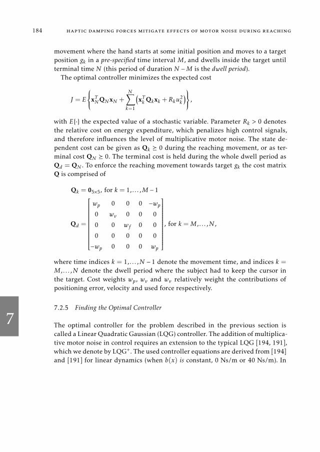
7
184 haptic damping forces mitigate effects of motor noise during reaching
movement where the hand starts at some initial position and moves to a target
position gk in a pre-specified time interval M , and dwells inside the target until
terminal time N (this period of duration N −M is the dwell period).
The optimal controller minimizes the expected cost
J = E
xTNQNxN +
N∑
k=1
(
xTk Qkxk +Rku2k
)
,
with E· the expected value of a stochastic variable. Parameter Rk > 0 denotes
the relative cost on energy expenditure, which penalizes high control signals,
and therefore influences the level of multiplicative motor noise. The state de-
pendent cost can be given as Qk 0 during the reaching movement, or as ter-
minal cost QN 0. The terminal cost is held during the whole dwell period as
Qd = QN . To enforce the reaching movement towards target gk the cost matrix
Q is comprised of
Qk = 05×5, for k = 1, . . . ,M − 1
Qd =
wp 0 0 0 −wp
0 wv 0 0 0
0 0 wf 0 0
0 0 0 0 0
−wp 0 0 0 wp
, for k =M , . . . ,N ,
where time indices k = 1, . . . ,N − 1 denote the movement time, and indices k =
M , . . . ,N denote the dwell period where the subject had to keep the cursor in
the target. Cost weights wp , wv and wv relatively weight the contributions of
positioning error, velocity and used force respectively.
7.2.5 Finding the Optimal Controller
The optimal controller for the problem described in the previous section is
called a Linear Quadratic Gaussian (LQG) controller. The addition of multiplica-
tive motor noise in control requires an extension to the typical LQG [194, 191],
which we denote by LQG+. The used controller equations are derived from [194]
and [191] for linear dynamics (when b(x) is constant, 0 Ns/m or 40 Ns/m). In
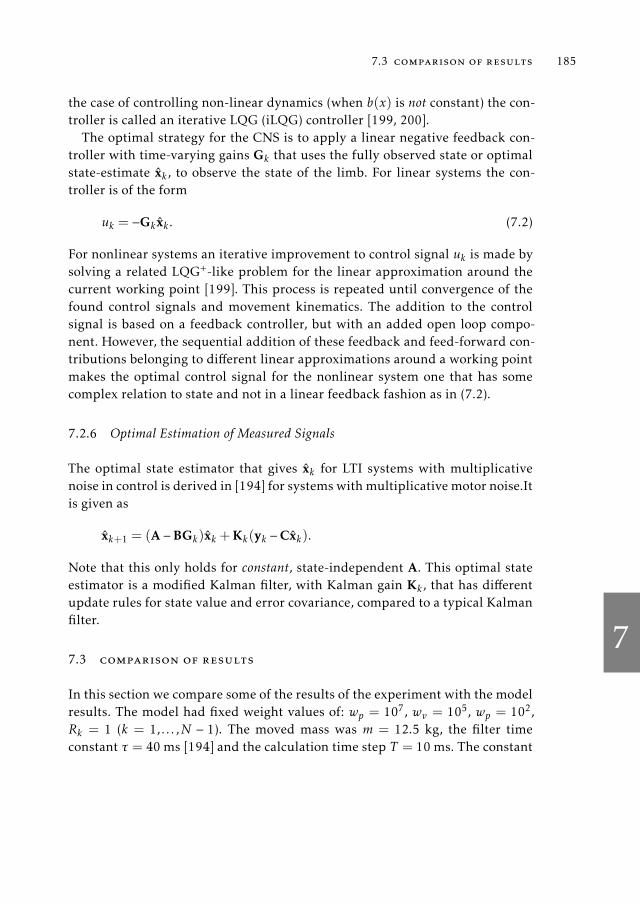
7
7.3 comparison of results 185
the case of controlling non-linear dynamics (when b(x) is not constant) the con-
troller is called an iterative LQG (iLQG) controller [199, 200].
The optimal strategy for the CNS is to apply a linear negative feedback con-
troller with time-varying gains Gk that uses the fully observed state or optimal
state-estimate xk , to observe the state of the limb. For linear systems the con-
troller is of the form
uk = −Gk xk . (7.2)
For nonlinear systems an iterative improvement to control signal uk is made by
solving a related LQG+-like problem for the linear approximation around the
current working point [199]. This process is repeated until convergence of the
found control signals and movement kinematics. The addition to the control
signal is based on a feedback controller, but with an added open loop compo-
nent. However, the sequential addition of these feedback and feed-forward con-
tributions belonging to different linear approximations around a working point
makes the optimal control signal for the nonlinear system one that has some
complex relation to state and not in a linear feedback fashion as in (7.2).
7.2.6 Optimal Estimation of Measured Signals
The optimal state estimator that gives xk for LTI systems with multiplicative
noise in control is derived in [194] for systems withmultiplicative motor noise.It
is given as
xk+1 = (A−BGk)xk +Kk(yk −Cxk).
Note that this only holds for constant, state-independent A. This optimal state
estimator is a modified Kalman filter, with Kalman gain Kk , that has different
update rules for state value and error covariance, compared to a typical Kalman
filter.
7.3 comparison of results
In this section we compare some of the results of the experiment with the model
results. The model had fixed weight values of: wp = 107, wv = 105, wp = 102,
Rk = 1 (k = 1, . . . ,N − 1). The moved mass was m = 12.5 kg, the filter time
constant τ = 40 ms [194] and the calculation time step T = 10 ms. The constant
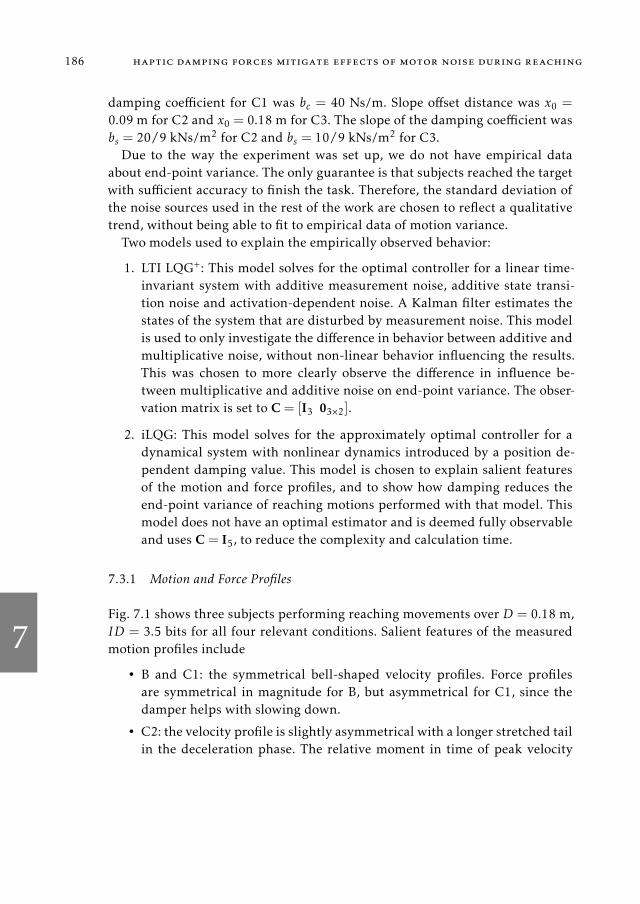
7
186 haptic damping forces mitigate effects of motor noise during reaching
damping coefficient for C1 was bc = 40 Ns/m. Slope offset distance was x0 =
0.09 m for C2 and x0 = 0.18 m for C3. The slope of the damping coefficient was
bs = 20/9 kNs/m2 for C2 and bs = 10/9 kNs/m2 for C3.
Due to the way the experiment was set up, we do not have empirical data
about end-point variance. The only guarantee is that subjects reached the target
with sufficient accuracy to finish the task. Therefore, the standard deviation of
the noise sources used in the rest of the work are chosen to reflect a qualitative
trend, without being able to fit to empirical data of motion variance.
Two models used to explain the empirically observed behavior:
1. LTI LQG+: This model solves for the optimal controller for a linear time-
invariant system with additive measurement noise, additive state transi-
tion noise and activation-dependent noise. A Kalman filter estimates the
states of the system that are disturbed by measurement noise. This model
is used to only investigate the difference in behavior between additive and
multiplicative noise, without non-linear behavior influencing the results.
This was chosen to more clearly observe the difference in influence be-
tween multiplicative and additive noise on end-point variance. The obser-
vation matrix is set to C= [I3 03×2].
2. iLQG: This model solves for the approximately optimal controller for a
dynamical system with nonlinear dynamics introduced by a position de-
pendent damping value. This model is chosen to explain salient features
of the motion and force profiles, and to show how damping reduces the
end-point variance of reaching motions performed with that model. This
model does not have an optimal estimator and is deemed fully observable
and uses C= I5, to reduce the complexity and calculation time.
7.3.1 Motion and Force Profiles
Fig. 7.1 shows three subjects performing reaching movements over D = 0.18 m,
ID = 3.5 bits for all four relevant conditions. Salient features of the measured
motion profiles include
• B and C1: the symmetrical bell-shaped velocity profiles. Force profiles
are symmetrical in magnitude for B, but asymmetrical for C1, since the
damper helps with slowing down.
• C2: the velocity profile is slightly asymmetrical with a longer stretched tail
in the deceleration phase. The relative moment in time of peak velocity

7
7.3 comparison of results 187
00.25
0.5
0.75
10
0.05
0.1
0.15
0.2
0.25
Subject7:Pos.[m]
00.25
0.5
0.75
1−0
.250
0.25
0.5
0.751
Vel.[m/s]
BC1
C2
C3
00.25
0.5
0.75
1−1
00
−500
50
100
Force[N]
(a)
00.25
0.5
0.75
10
0.05
0.1
0.15
0.2
0.25
Subject14:Pos.[m]
00.25
0.5
0.75
1−0
.250
0.25
0.5
0.751
Vel.[m/s]
00.25
0.5
0.75
1−1
00
−500
50
100
Force[N]
(b)
00.25
0.5
0.75
10
0.05
0.1
0.15
0.2
0.25
MT[s]
Subject18:Pos.[m]
00.25
0.5
0.75
1−0
.250
0.25
0.5
0.751
MT[s]
Vel.[m/s]
00.25
0.5
0.75
1−1
00
−500
50
100
MT[s]
Force[N]
(c)
Figure
7.1:a–c)
Meanresu
ltsforID
=3.5
bits,
D=
0.18m,shad
edarea
shows±1
stan
darddev
iation.Thelegen
din
the
top-cen
tersu
bfigure
applies
toallsu
bfigures.a)
Subject
7,b)Subject
8,c)
Subject
18.

7
188 haptic damping forces mitigate effects of motor noise during reaching
0 0.25 0.5 0.75 10
0.05
0.1
0.15
0.2
0.25
MT [s]
Pos.[m
]
(a)
0 0.25 0.5 0.75 1−0.250
0.25
0.5
0.75
1
MT [s]
Vel.[m
/s]
B C1
C2 C3
(b)
0 0.25 0.5 0.75 1−100
−50
0
50
100
MT [s]
Force[N
]
(c)
Figure 7.2: a) position profiles, b) velocity profiles, and c) force profiles produced by theiLQGmethod and the non-linear dynamical model. Dwell time starts at: 0.55s for B, 0.525 s for C1, 0.475 s for C2 and at 0.425 s for C3, indicated with acolored dashed line. Notice the same asymmetry in the velocity profiles forC2 (longer right tail) and C3 (sharp drop-off on the right) as is visible in theexperimental data in Fig. 7.1. The legend in b) applies to all subfigures.
is earlier, compared to B and C1. Furthermore, there is no need for the
subjects to apply a deceleration force.
• C3: the velocity profile is asymmetrical, with a ‘sharp bend’ near the peak
velocity with fast deceleration. The relative moment in time of peak veloc-
ity is later, close to the onset of the damping. Force profiles are asymmet-
rical in magnitude since the damper helps in slowing down.
Fig. 7.2 shows the outcomes of noise-free nonlinear models, solved with the
iLQG method. All salient features shown in the experimental data are visible
in the model results: the asymmetry in force profile magnitude, the asymmetry
in velocity bell-shapes for C2 and C3. Although the first observation about force
asymmetry might be thought of as a trivial result of complementing the damper
force, the velocity and force profile time asymmetries are visible results from an
optimization process. This comparison hints at the fact that reaching motions
subjected to time-varying damping can be well explained and predicted by op-
timization methods such as optimal control. It shows that humans re-optimize
their movement plan for the different dynamical conditions.

7
7.3 comparison of results 189
0.4 0.6 0.8 1
10−4
10−3
10−2
MT [s]
SD
Reach
ingPosition[m
]
σu = 0.0001
(a)
0.4 0.6 0.8 1
MT [s]
σu = 0.001
(b)
0.4 0.6 0.8 1
MT [s]
σu = 0.01
B C1
C2 C3
(c)
Figure 7.3: a–c) For different multiplicative noise scaling factors σu : the standard devia-tion in reached end-point position taken from 40movement repetitions of theiLQGmethod and the non-linear dynamical model at the end of the dwell pe-riod, for different MT. Reaching distance was 18 cm. The legend in c) appliesto all subfigures.
7.3.2 Influence of Noise Variance
Multiplicative Noise and Fitts’ Law
The nonlinear dynamical model was run with activation-dependent noise with
three different unitless noise standard deviation scaling values σu = 0.0001,
0.001 and 0.01 in (7.1). The MT of the reaching motion was varied from 0.3
to 1.0 s with added dwell time of 0.5 s. The model was run 40 times to get a
measure of end-point accuracy in the form of standard deviation in reaching
position.
The numerical results of these models are shown in Fig. 7.3. Fitt’s Law behav-
ior is observed in the increased accuracy, smaller end-point position standard
deviation, for longer MT. Also, all damping conditions increase the model’s end-
point accuracy. This might explain the reducedMT for conditions C1, C2 and C3
observed in the experiment. To achieve similar reaching accuracy for e.g. C1 as
in B, we notice that this movement can be performed with less MT. This relative
trend between conditions is true for all values of σu .

7
190 haptic damping forces mitigate effects of motor noise during reaching
0.4 0.6 0.8 1
10−4
10−3
10−2
0.3 0.5 0.7 0.9
MT [s]
SD
Reach
ingPosition[m
]
BM C1MBA C1A
Multiplicative Noise
Additive Noise
Figure 7.4: Additive process and measurement noise (subscript ‘A’ for additive, dashedlines) in the LQG+ model shows that for larger MT the end-point varianceincreases. This is different from neural activation dependent noise (subscript‘M’ for multiplicative, solid line). Damping forces filter contributions of allnoise sources. The model results were averaged over 10,000 movement repe-titions.
Notable is the fast decrease in variance for the C3 condition, with a minimal
value at a MT of 0.6 s. It is not known whether minimal variance would happen
in real reaching tasks with that MT. Nevertheless, demanding a slow movement
through an increasing damping field might require more neural activation for a
longer time, which in turn actually reduces end-point accuracy.
Additive Noise versus Multiplicative Noise
To investigate the relative effect of multiplicative and additive noise on end-
point variability for LTI dynamics B and C1 only, the model was run with either
a) multiplicative motor noise (σu = 0.3), or b) a combination of additive obser-
vation noise and process noise (σw = 5 N, σv = [0.025 m,0.1 m/s,6.5 N]T , the
parameter values were chosen to deliver similar movement variance visually, as
the observed variance during motions used to produce Fig. 7.3. The MT of the
reaching motion was varied from 0.3 to 1.0 s with added dwell time of 0.5 s. The
model was run 10,000 times to get a measure of end-point accuracy in the form
of standard deviation in reaching position.
The quantitative difference between the influence of additive and multiplica-
tive noise (and therefore the exact used values for noise variance) are irrelevant
in this example, because we are merely interested in the trend of the end-point
variance versus MT and how this changes between conditions. The end-point

7
7.4 discussion and future work 191
variance increases with MT for additive noise, as is shown in Fig. 7.4. This trend
is in contrast to the trend for dynamics with multiplicative motor noise alone. It
would imply that taking a longer MT would result in less accurate movements.
This is neither in accordance with Fitts’ Law, nor with observation. Therefore, a
model with large additive noise cannot be a model that describes the variance
features of our reaching dynamics. Nevertheless, some amount of additive noise
is unavoidable in the real motor system.
Added damping forces reduced end-point variance for both themultiplicative
noise (this is a reconfirmation of the iLQG results for B and C1 in Fig. 7.3) as
well as for additive noise. The human motor system is contaminated by more
sources of noise than just a single multiplicative noise source. Damping forces
might therefore also reduce contributing effects of other sources of noise.
7.4 discussion and future work
The aim of this work was to give qualitative evidence from computational mod-
els to support the hypothesis that damping reduces end-point variance, allows
for moremotor activation and therefore reducesMT for fast reaching tasks [179].
Performing optimally controlled movements with the same cost function and
same MT shows reaching kinematics with smaller end-point variance in condi-
tions C1, C2 and C3. This corroborates results we presented in [179] (see Chap-
ter 6). Salient features of motion and force profiles of the models are highly sim-
ilar to experimental data. This is a strong indicator that the models used, and
therefore also their response to noise, are an indicator of why subjects managed
to reduce their reaching time. Damping force gives subjects the possibility to in-
crease their neural activation and move faster, since it allows them to guarantee
a certain targeting variance.
The experimental results, andmodel results agree with the hypothesis in [168]
that the use of friction or damping, in general, shows a noise filtering behavior.
Our used models give insight into how this filtering effect happens. The results
and model agree with our hypothesis that MT can be reduced because subjects
exploit the variance-reducing effect of the damping force, because the task in-
struction was to move as fast as possible.
Another way to think about the benefit of constant damping or PDD is that
it acts as an antagonist muscle whose activation is noise-free and does not con-
tribute to increasing the end-point variance. If this virtual antagonist muscle is

7
192 haptic damping forces mitigate effects of motor noise during reaching
‘tuned properly’ to activate during a required deceleration or targeting phase, it
benefits the subject.
7.4.1 Alternative View and Possible Falsification
A second possible explanation, somewhat in line with the previous statement, of
the decrease in MT for the damping conditions could be ascribed to implicit role
distribution of the subject with the damping field. One could suggest that the
subject considered the damping field as another ‘agent’ which aided the subject
in te reaching movement by assisting in the deceleration phase of the movement.
Reed et al. [201] showed that two human partners working together on a target
acquisition task performed the task faster than individuals performing the same
task. Through the recorded interaction forces, they observed specialization, in
which one partner accelerated and the other partner decelerated the movement.
The specialization was hypothesized to be the cause of the faster reaching move-
ment [201]. However, the authors could not explain a mechanism behind the
benefit of this role distribution.
To investigate this hypothesis, multiplicative force noise could be added to
the damping force, i.e. noise that scales with the velocity state. According to our
hypothesis, this should in turn increase MT. If this does not happen, however,
it might be more indicative of benefits of human-human role distribution. Al-
though this does not explain why this role distribution, with two agents that
are both influenced by their own multiplicative motor noise, would result in a
shorter MT.
7.4.2 Model and Method Limitations
The used optimal control reaching models do have their limitations and draw-
backs. For physical reaching movements, the MT is an outcome metric of the
performed actions. However, in the model, the MT is a predefined parameter. A
similar issue is raised in [202] where they ascribe slower movements of Parkin-
son’s disease patients to higher cost on energy. The high cost on energy would
henceforth increase MT. However, a model with fixed MT does not show this
behavior with different cost on energy expenditure.
This problem can be overcome by adding a non-zero state-dependent cost dur-
ing the reaching motion before the dwell period. However, this would put more
cost on being far away from the target, and less cost on being close. This is dif-

7
7.4 discussion and future work 193
ferent from the more reasonable idea of only inducing cost when not ending up
at the target. Also, state dependent cost during reaching results in highly asym-
metrical velocity and force profiles that are not observed in human reaching.
However, cost during a dwell period or at terminal time does resemble human
reaching kinematics very well.
For a Fitts’-like reaching task the state dependent cost could be made some-
thing highly nonlinear, similar to (|D−x(t)| <W/2)+energy cost, withD andW
the reaching distance and target diameter respectively. The Boolean expression
on the left would force the arm to reach the target with the demanded accuracy
without differently penalizing distance from the target. Reweighting the energy
cost would directly influence the found MT. However, such a non-linear cost
has no proper derivative in state, and is therefore hard to apply in the iLQG
setting where the non-linear cost is approximated by a quadratic cost in the
linearization. Different solution strategies, like evolutionary optimization meth-
ods to find a parameterized control signal might be able to handle such a cost
function better than the current methods.
The results of both the experiment and the model are also limited in that they
cannot be extrapolated to arbitrary weights and arbitrary damping force magni-
tude. Amore realistic muscle model with force saturation would be a straightfor-
ward extension to identify how humans would re-optimize their reaching strat-
egy for interacting with such heavy mechanical mass or high damping force that
they require peak voluntary muscle contraction.
7.4.3 Experimental Limitations and Recommendations
The currently performed experiment was set up mainly to determine how sub-
jects’ MT would change for all the damping conditions, compared to a no damp-
ing condition. The used protocol was not ideal to extract the information to
explain the applied strategies with optimal control. There was no comparable
measure of end-point accuracy to compare to the model results.
A Fitts’ like reaching experiment that demands subjects to dwell in the tar-
get introduces more variance in MT than in tapping tasks [179]. A dwell time
measurement also eliminates a proper measure of end-point variance. In future
research, a more typical two-way tapping task or button-press task, but with
high mass, might serve two useful purposes: 1) giving a proper measure of end-
point variance, 2) give a better fit to Fitts’ law.

7
194 haptic damping forces mitigate effects of motor noise during reaching
Future research might focus more on single distance reaching with e.g. only
two target sizes to remove any variance due to target distance and target size.
All non-baseline conditions could have constant damping, with smaller steps
in value between conditions. This might give more insight in how subjects re-
optimize their movement, and (with a better cost on state, or terminal state)
possibly how it can be explained with a relative reweighting between targeting
error and energy expenditure.

7
7.4 discussion and future work 195


Part IV
GENERAL CONCLUS IONS


8
8DISCUSS ION
This dissertation presented several studies towardsmethods to improve exoskele-
ton and interaction devices that physically support humans. The following three
questions guided the research process:
Research Questions
I. How to support the full range of motion of the human shoulder?
II. How to implement stable admittance control with inertia reduc-
tion?
III. How do humans respond to dissipative shared control forces?
In this chapter the work presented in this dissertation will be reiterated and dis-
cussed, especially focusing on scientific contribution and context, other possible
applications, limitations of the presented work and possible future development
and research directions.
8.1 supporting the range of motion of the human shoulder
Chapter 2 presented a method to visualize the range of motion (ROM) of the
three degrees of freedom (DOF) of rotations of the human glenohumeral (GH)
joint. The visualization allows us to show the three DOF on a two-dimensional
plane for easier communication and publication of results.
The method allows for a visual comparison of ROM between humans, healthy
subjects and patients, between a human and a device (like an exoskeleton) or
between devices. Colors were used to show kinematic conditioning of exoskele-
tons, although it is possible to show other parameters such as device inertia, ap-
plied forces, movement time, movement accuracy or translations of the shoulder
girdle by varying colors, varying circle radii and multiple circles.
Due to the movement of the scapula at the scapulothoracic joint, and the clav-
icle at the sternoclavicular and acromioclavicular joint, the shoulder can also
translate by performing up and downward motions (elevation and depression),
199

8
200 discussion
and forward and backward motions (protraction and retraction). The presented
work focuses solely on pure rotations of the GH joint, neglecting these transla-
tional motions. Nonetheless, the method could be expanded to show these two
extra DOF in translation as arrows or lines in the circle centers, for example.
Scientific Contribution and Context
Compared to other methods to present shoulder ROM in literature, our method
is able to show how the ROM is coupled between different movement directions
in a single non-ambiguous 2D figure. In literature, the shoulder ROM is mostly
presented along along the fivemedical directions of motion alone. This results in
a workspace that is not representative of the actual human workspace; making
the workspace too small in some configurations and too large in others. This is
a serious problem during assistive device design and device evaluation where
devices cannot exceed human ROM due to safety reasons.
Presenting merely the ROM of five medical directions also limits the com-
munication of proper ROM during evaluation of how human shoulder ROM is
affected by different movement pathologies.
Compared to projected 3D visualizations of the elbow-tip, our method shows
axial rotation readily and does not suffer from projection ambiguity.
Our method also allows to show and compare kinematic, dynamic of perfor-
mance metrics of humans and devices directly and intuitively, something that
was not possible with other methods.
Further Application
The visualization method is not limited to the rotational ROM of the GH joint,
but could be used for other three DOF rotation joints. Candidates for such dis-
play are the hip joint, the ankle joint and the complex combinations of joints in
the wrist and elbow that provide the wrist with effectively three DOF.
Furthermore, the visualizationmethod is useful to display the rotational ROM
of non-anthropomorphic robots and mechanisms in general. This is commonly
still shown as a (multi-)projected ambiguous 3D image of a workspace boundary,
losing information about coupling within ROM.
Limitations
A minor drawback of the presented method is the required quantization of GH
horizontal and GH elevation rotation, to avoid visual overlap between the circles
8
8.1 supporting the range of motion of the human shoulder 201
of GH axial ROM. However, the grid can be made as finely spaced as preferred,
or can be made non-uniform if specifically interesting areas of interest need to
be shown.
The ROM presented in Fig. 2.1 is large. This might be influenced by inaccu-
rate measurements done with a goniometer. Work was done [203], albeit not
presented in this dissertation, where we measured the shoulder ROM with two
inertial measurement units; one on the sternum and one on an elbow that was
fixed in a 90 degrees flexion angle. This allowed for the measurement of relative
rotation between the upper body and the upper arm, which equals the shoul-
der rotation. The subject would ‘point’ his/her elbow to a point on the grid and
then traverse the complete axial-rotation ROM. This process was repeated for all
grid intersections. Different measurement protocols were evaluated that build
complete ROM diagrams similar to those in Chapter 2. This method showed a
smaller ROM than in 2.1, especially in axial GH-rotation and horizontal GH-
rotation. During this work we noticed that measuring the ROM of the shoulder
for a visualization as presented in Chapter 2 is intensive, and somewhat painful,
even for healthy subjects. For patients with shoulder pain or limb weakness,
intensive measurements that map the complete ROM like done here might be
unfeasible. However, the problem of painful ROM measurement is not unique
to this specific measurement and visualization method.
Future Research
Future work includes the quantitative evaluation of several case studies where
ROM of the human shoulder and devices is presented in the new method and
along the five medical directions of motion. In this way it is possible to get an
expert opinion on using the method to communicate ROM and device proper-
ties. Furthermore, it is possible to quantify how much error is introduced by
presenting the range of motion along the five medical directions, compared to
presenting it in our new method.
Future work should also include an investigation into whether the history of
motion influences the measured ROM in certain upper arm configuration.
Chapter 3 presented a conceptual kinematic design for a four DOF (or 4R)
shoulder exoskeleton where the exoskeleton axes are non-orthogonal (i.e. if a
more dominant joint rotates, the motion of the following joint axis describes an
obtuse or acute cone, instead of a flat circle). Such a shoulder exoskeleton can be
used to increase the ROM of conventional 3R exoskeletons by having more pos-
8
202 discussion
sibilities to avoid collisions with the human body and avoid configurations with
poor kinematic conditioning. Both of these problems limit the usable workspace
current 3R exoskeleton designs.
The proposed 4R shoulder exoskeleton shoulder supports the GH rotations
of the shoulder, while translations due to elevation, depression, protraction and
retraction are taken care of by a separate translation mechanism that is placed
in series, kinematically speaking in front of the joint, closer to the system’s base.
We required an inverse kinematics (IK) solution method to calculate reference
joint angles from non-prescribed motion trajectories. Such trajectories can be
derived from real-time interaction control methods. Especially admittance con-
trol prescribes motions to an interaction device, such as an exoskeleton, after a
user applies forces onto the device. Since these inputs are not known a-priori, a
flexible solution strategy was needed.
Scientific Contribution and Context
We found that any 3R or 4R exoskeleton can support all 3D rotations (i.e. cover
all of SO(3) at least once) if and only if the sum of absolute differences between
the angles-between-exoskeleton-axes and 90 degrees is smaller than, or equal
to 90 degrees. This allows for a non-orthogonal joint design that can assist in
avoiding body and internal collisions, compared to an orthogonal design, but
achieve all possible rotations.
We chose to develop and evaluate a differential non-unique solution to the
IK problem, instead of developing a direct unique 3DOF arm configuration to
unique 4DOF joint-configurationmapping (i.e. a non-differential angle-to-angle
mapping). The main reason for this is that for an angle-to-angle mapping the
method becomes a look-up-table that needs to interpolate 3D rotations between
arm configurations. Furthermore, such a method does not allow the exoskeleton
to move to a configuration further away from the body and from singularity
when the person inside the exoskeleton is not moving their arm.
Because the exoskeleton joint is redundant by one degree of freedom, a one
dimensional self-motion-manifold (SMM) allows for internal motions of the
joint that do not influence the motion or configuration of the human arm. Our
method exploits this self-motion to continuously steer away from exoskeleton
singularity and body collisions, as is shown for a specific conceptual exoskele-
ton design as a test case.
To guarantee that the exoskeleton joint would always steer away form the
body and singularity fast enough, given some limit on input speed, a newmethod
8
8.1 supporting the range of motion of the human shoulder 203
is used to converge along the SMM to a ‘better’ configuration. This method over-
comes issues found in gradient projection of secondary movement objectives,
which can get stuck in a local minimum. However, for sufficiently slow move-
ments, and careful analysis, a gradient projection might be sufficient for a spe-
cific exoskeleton design. Furthermore, if a sufficiently complex gradient (or its
potential) would be constructed, gradient projection and our newmethodwould
be identical. However, parameterizing a potential function to have a gradient
that is always parallel and never perpendicular to the SMM is complicated.
The shown method assumed an instantaneous center of rotation inside the
human GH joint. This is, however, not necessarily required. The methods also
applies to an exoskeleton design where the axes of rotation do not intersect in
the same point, or do not intersect at all. This could be the case if the fourth
degree of freedom is parallel to the axial rotation of the upper arm, but with a
translational offset. However, the collision constraints then become dependent
on the fourth joint angle, which makes the analysis more involved.
The analysis method described in the chapter can also be used to develop in-
verse kinematics strategies for redundant designs with passive internal degrees
of freedom. However, a solution might not always exist for any arbitrary design.
Further Application
The proposed method is also usable for generic 4R joints that need to steer away
from poor kinematic conditioning or collisions with the fixed world. A related
problem could be the one of shoulder joints in humanoid or bio-inspired robots
and hip-joints in exoskeletons and humanoid or bio-inspired robots.
Limitations
This research was mainly an investigation into whether a full range of motion
exoskeleton is achievable in principle. An exoskeleton that can support the full
human (shoulder) ROM is a luxury and usually not a necessity for many power
augmentative tasks such as the support of healthy workers or support of rehabil-
itating patients. Especially the latter group might not benefit from a larger ex-
oskeleton ROM, whereas the device complexity of the device and reliability on
the software would be substantially increased. Enforcing end-of-ROM in such a
device is crucial to not overextend the human (patient’s) shoulder. This problem
is challenging formore typical 3R designs, but becomesmore difficult, and relies
more on software safety, for 4R designs. However, we speculate that increasing

8
204 discussion
the ROM of an exoskeleton to fit the human ROM increases user acceptance and
could be especially useful for industrial, or agile military tasks.
Future Research
Future research should investigate possibilities and integration methods to per-
form the samemethod in the acceleration domain instead of the velocity domain.
In that way the velocities can be made smooth, which is beneficial for joint mo-
tion tracking by low-level motion controllers.
Future work should also include better mechanical design than the proposed
concentric arcs used in the presented conceptual prototype. Furthermore, a real-
istic solution has to be incorporated to place the fourth degree of rotation inside,
or parallel to the upper arm. In a practical design there might not be a single
center of rotation where all rotation axes intersect. This results in translations
of the device, which demands possibly different joint-space constraints that the
method should conform to.
8.2 implementing stable admittance control with inertia reduc-
tion
Chapter 4 presented admittance control as an interaction control paradigm. Ad-
mittance control requires a force sensor to measure the interaction forces be-
tween the human operator and the robot. This is commonly referred to as ‘de-
tecting the intent of the user’ that lets the device know where to move. The mea-
sured forces are used as an input to a virtual dynamical model that calculates
the desired robot motion state. A motion controller tries to control the robot
motion to follow this desired state. In this way the robot can be programmed to
behave like, and feel like, the virtual model.
Admittance control can be used to reduce inertia of heavy devices if the vir-
tual model has a lower inertia than that of the real device. This is a relevant
strategy for heavy lifting devices, as well as for rehabilitation and supportive
robots. In all these cases the device or load is too heavy and too inert to move
easily by the operator. In such cases admittance control acts as a method of
power augmentation.
Compared to impedance controlled devices, feedback-only admittance con-
trol does not need models of the robot’s parasitic effects, such as friction and par-
asitic dynamics, to simulate desired virtual dynamics. In practice, especially in-

8
8.2 implementing stable admittance control with inertia reduction 205
ertia reduction is more straightforward to perform on an admittance controlled
device than on an impedance controlled device. An impedance controlled de-
vice would need to estimate or measure accelerations that result in noisy anti-
inertial forces. During admittance control, interaction force is measured that is
passed through a model of virtual dynamics, that effectively filters noise contri-
butions and allows for more smooth interaction. Furthermore, admittance con-
trol can almost trivially render stiffness and damping dynamics in a stable and
passive way, because it is always motion controlled (see the analysis performed
in the chapter). For example: simulating hard contact with admittance control is
merely a change of motion state in the virtual model that the motion tracker has
to follow, regardless of whether the device is inside or outside of that wall. There-
fore, if the motion reference (the model) is not ejected from the wall, neither is
the device. An impedance controller, however, generates a spring-damper force
inside the wall, but no force outside it. Therefore a used device might be ejected
out of the wall by that spring and bounce or shoot away when time quantization
steps are too coarse, resulting in free floating, uncoupled, instability.
If the inertia of the robot is reduced by an admittance controller, the robot can
become unstable when the force sensor comes in contact with, or is coupled to, a
stiff environment. This is a relevant problem when a human operator holds and
moves a device, or is attached to a device such as an exoskeleton. Possible muscle
co-contraction and intrinsic limb properties introduce a non-zero amount of
joint, limb and interface stiffness for the device to interact with.
This kind of coupled instability can be explained as non-passive, or active,
behavior of the robot. The idea behind the energy passivity property of dynami-
cal systems is that such systems cannot generate energy and are therefore stable
during physical interaction with other passive systems. Any possible intercon-
nection of passive systems is consequently also stable. If the admittance con-
trolled device can be made to behave energetically passive, it is guaranteed to
be stable when in contact with the (passive) human limb, and from everyday
experience we realize that human interaction with passive objects is generally
stable.
Imposing that a device behaves passively could be seen as being conserva-
tively stable. Being passive implies interaction stability for an admittance con-
trolled device coupled to infinite human stiffness, although the human’s interac-
tion stiffness in practical applications is limited and finite. Nonetheless, passiv-
ity conditions give relevant design goals that should be aimed for when aspiring
interaction stability over a large range of device and environment impedance.

8
206 discussion
Because if the preferred dynamics can be achieved while being passive and
while compensating for disturbances, then both interaction stability and per-
formance goals are achieved simultaneously.
Scientific Contribution and Context
Passivity conditions for controlled linear time-invariant systems are derived
from the positive real condition (PRC), made popular by Colgate [92]. The PRC
gives ‘black box’ frequency domain passivity conditions that put limits on the
values of system and control parameters to guarantee that the admittance con-
trolled robot behaves passively. The PRC, however, does not explain what causes
the active behavior.
For admittance control with inertia reduction, and feedback motion control
only, the PRC states that effectively no passive inertia reduction can be achieved.
If attempted, there will always be some interaction stiffness of the human limb
that will destabilize the interaction. Adding a constant amount of virtual damp-
ing allows for more integral velocity gain (i.e. more position control gain) to be
used in the motion controller, allowing for a better low frequency approach of
the intended lowered inertia. The amount of inertia that can be reduced in that
way, however, is limited to few percent at most in any practical application.
The design guidelines we derive from the PRC all point in the same direc-
tion: 1) minimize phase lag between the measured force and resulting motion
of the robot and 2) achieve as high motion control bandwidth as possible. The
former limits any allowable low-pass filtering of force signals and puts limits on
internal compliance of the robot. The latter tells us to use as much feed-forward
(computed torque, or inverse dynamics) control, possible acceleration feedback
or control, reduce loop-delay time and to use high sampling rates for the con-
troller and updates of the virtual dynamics. Closed-loop feedback control is
still required, however, to reject friction and other unmodeled disturbances that
would have an otherwise parasitical effect on the felt robot impedance.
Even if the inertia of the robot is reduced towards the inertia of the virtual
model, cuffs, handles or tools attached to the force sensor still introduce extra
inertia and weight that is felt by both the force sensor and the user. This post-
sensor inertia can be compensated with acceleration feedback by feeding back
a fake force signal that reduces the contribution of inertial forces on the device.
However, this is a method of positive feedback, and the PRC rightfully states
that this reduces the stability margins.
8
8.2 implementing stable admittance control with inertia reduction 207
Further Application, Limitations and Future Research
The guidelines presented can be used to design haptic simulation devices or
tools for heavy lifting in industrial and health-care scenarios.
The work presented, however, is limited to linear single DOF robots. Further-
more, the post-sensor dynamics were assumed to be purely inertial. If the post-
sensor dynamics have a resonant mode or significant play, handling that be-
havior might be more difficult, even though its behavior is supposedly passive.
Investigation is needed into whether different kinds of post-sensor dynamics
result in different guidelines.
Future work would need to expand more on multi-DOF robots and robots
with internal compliance. The work has to be more extensively compared with
the pioneering work of Colgate [89] that states that any kind of internal com-
pliance puts fundamental limits on the amount of passively achievable inertia
reduction for any kind of controller.
Chapter 5 presented an analysis into the active nature of admittance control
and developed a time-domain control method, called SPIS, to dissipate the en-
ergy that causes this instability.
Scientific Contribution and Context
The PRC is a black box condition that does not explain the source of active be-
havior in admittance control. A time-domain analysis shows that admittance
control is not (strictly) passive due to energy created as a result from the power
conjugation of velocity tracking error and the interaction force. This corrobo-
rates the idea that for admittance control the motion tracking should have high
bandwidth, which would reduce velocity tracking error and in turn reduce the
amount of generated energy.
From a system’s perspective, an outer loop has to be closed to copy the mea-
sured force to the virtual dynamics, which is unilaterally connected to the mo-
tion controller. This unilateral connection, and the outer loop, break the ‘energy
consistent nature’ of the control method as a whole. This results in unstable in-
teraction of an admittance controlled robot with stiff environments, even with-
out reduced stability margins due to time-discretization.
This shows that other methods proposed in literature (i.e. in [145, 146]) can-
not make admittance control with inertia reduction passive in the time-domain.
The apparent success of time-domain passivity enforcement on open-loop
impedance controlled devices has been the fact that impedance controlled sys-
8
208 discussion
tems are dynamically ‘energetically consistent’. The virtual dynamics (commonly
spring-damper combinations) are, albeit discrete-time, passive elements that fit
in a physically consistent chain of systems that exchange energy. Instability then
arises due to the time-discretization of these systems.
Dissipating the exact amount of energy generated with time-varying damper
on the virtual model and the motion controller could also lead to passive be-
havior for admittance control with inertia reduction. However, this requires dy-
namic changes to, or read-outs of, a low level motion controller, whichmight not
always available for motors with closed drive systems. Therefore, we attempted
to achieve interaction stability by damping away excess energy from the vir-
tual dynamics alone. However, because the virtual (desired) velocity from the
virtual model can become arbitrarily small, it cannot be guaranteed to exactly
dissipated the generated energy during each sample. Therefore, this method can
only guarantee stability but not passivity.
The proposed SPIS method switches on a constant damper if the kinetic en-
ergy stored in the virtual model exceeds the energy introduced by the human
operator. This stabilizes any unstable interaction. If the interaction was already
passive, or if the device is free-floating, the damper does not need to intervene.
Therefore the damper only switches on as a ‘safety layer’ when required.
Further Application
SPIS can be used as a last-resort safety layer for admittance controlled devices
interacting with humans that would otherwise exhibit coupled instability in cer-
tain configurations or conditions.
Limitations and Future Research
The proposed method focused on simulating solely inertial virtual dynamics.
Furthermore, it does not allow to perform useful work (i.e. that the device moves
a human limb along a trajectory), since that would violate a strict passivity re-
quirements. This latter problem is readily overcome by introducing an energy
budget for these types of assistive movements. Future work might also look at
varying the damping value more smoothly, although stability proofs of such
method get more involved. Also, due to the possible absence of models of the
used device, it is not always known a priori how high the switching damping
value needs to be. Future work should point out if this maximum damping can
be made adaptive, based on the exchanged energy of the robot back to the user.
8
8.3 how humans respond to dissipative shared control forces 209
It is unknown how this method extends straightforwardly to flexible systems
that have non-collocated motion and force measurement. However, measure-
ments on the real haptic setup that has some lowest resonant mode below the
Nyquist frequency of the controller did not show any apparent negative influ-
ence due to internal compliance.
Future work should also look into how the method can be extended to achieve
not just stability, but exact marginal passivity at the human-robot interaction
port. This is not trivial, since it is unknown how to divide the amount of dissi-
pation required at the virtual model and the robot dynamics during closed-loop
interaction with stiffness-like environments.
8.3 how humans respond to dissipative shared control forces
Chapter 6 presented the evaluation of a simple haptic shared controller based
on damping forces around reaching targets that we call position dependent
damping (PDD). Such a PDD shared controller is useful in e.g. industrial pick-
ing and placement of (heavy) objects.
Scientific Contribution and Context
We found that objects could be placed more accurately and more quickly if the
reaching target area damped the motion. This is damping especially useful in
tasks where lifting is assisted, where human operators tend to overshoot mo-
tions due to reduced gravity [21]. The additional benefit of using damping forces
is that they can be also be generated by (almost) passive exoskeletons and lifting
devices that do not require active control of forces on exoskeleton joints. This is
a potential benefit of damping forces, compared to active potential forces that
are used in more conventional haptic guidance.
In the experiment discussed in Chapter 6, subjects were instructed and moti-
vated to move a mass of 12.5 kg as quickly as possible along a 1D line towards
a target with a predetermined accuracy. They had to stay inside the target for
500 ms to be counted as a successful hit. Such an experimental design fits in the
Fitts’ law experimental paradigm.
In the three conditions where subjects were subjected to damping forces, they
were able to reduce their movement time. Especially PDD around a reaching
target reduced movement time by over 40%. PDD also reduced the number of
required target overshoots and reentries by a factor of 4, increasing end-point
accuracy.

8
210 discussion
Fitts’ law linear regressions between ID and movement time showed that the
information-theoretical form of Fitts’ law seems to hold. However, this linear
fit is not the only possible fit to the data, and other non-linear curve param-
eterizations could have a lower residual sum of squared error than the linear
regression. The only valid conclusion that can be drawn is that there was in-
deed an accuracy-speed trade-off in this experiment. The conditions with damp-
ing forces assisted in this trade-off for the subjects, resulting in higher possible
movement speed and consequently shorter movement times.
Further Application
Using PDD could also be beneficial in rehabilitation settings or in assistive de-
vices for daily use to increase controllability and stability. Examples of an appli-
cation would be position dependent damping during table or object approaches.
Limitations and Future Research
The experiment was limited to 1D target approaches. To better resemble real
world tasks, 3D reaching motions, possibly including peg-in-hole tasks, could
show whether the positive contributions of PDD generalize to more degrees of
freedom. However, in 3D a target is approachable frommultiple directions. This
requires the damping coefficient to be not only PDD but also direction depen-
dent to not impede the user when a target is not necessarily approached.
Chapter 7 presented a hypothesis to explain the results observed in Chapter 6.
Scientific Contribution and Context
We hypothesize that the used constant and position dependent damping attenu-
ated the mechanical effects of especially multiplicative noise in the humans mo-
tor control system. Higher levels of neural activation results in more absolute
force noise from the muscles. Subjects were instructed to perform the reaching
task as quickly as possible while conforming to the accuracy requirement. Mul-
tiplicative motor noise in their motor system would prohibit subjects to achieve
higher accelerations to move faster. Because if they did, then the required end-
point accuracy could not be guaranteed. Damping forces, and especially damp-
ing around the reaching target, attenuate the mechanical effects of this multi-
plicative motor noise and reduce the positional variance of the end-point. Due
8
8.3 how humans respond to dissipative shared control forces 211
to the reduction in variance, the subjects can generate more muscle force and
perform the reaching movements faster than without any damping.
Stochastic non-linear optimal control models show agreement with measure-
ments of movement kinematics and interaction forces.
Further Application
Understanding how humans interact with dynamics, for example by stochas-
tic optimal control models, might allow designers to reverse engineer optimal
interaction dynamics for shared-control-like paradigms. In this case it would
allow the design of optimal damping ‘profiles’ to achieve a certain desired accu-
racy after initial learning. A practical real-world application would be the use
of such a force to manually place heavy products on fittings or into machines
more quickly and accurately. In such a scenario the user would be supported by
a device in terms of gravity support and dissipative forces to make positioning
easier, effectively reducing the effort and possibly increasing productivity and
product safety.
Limitations Future Research
The experimental design used in Chapter 6 was not ideal to draw definitive con-
clusions to explain the observed results. Future experiments should be specifi-
cally designed to look at adaptation and investigate optimal control performed
by the human subject. Furthermore, future experiments should quantify the
movement variance. Results from those experiments could strengthen or falsify
the current hypothesis.
For example, a future experiment where subjects tap on a surface or press
a button at the target site might give a better indication of end-point variance.
Performing the experiment with a single movement distance, but different tar-
get sizes might draw a clearer picture of prescribed end-point variance and the
maximal accelerations humans achieve.
Furthermore, artificial multiplicative force noise could be added to the PDD
force to investigate whether this henceforth increases movement time. If this
does not happen, it falsifies our hypothesis and might be more indicative of
benefits role-distribution found in human-human cooperation tasks. This does
not explain, however, the mechanism behind why this role distribution, with
two human agents both contaminated with multiplicative motor noise, would
result in shorter movement time.

8
212 discussion
Optimal Control and Haptic Shared Control
Within the H-Haptics project research was done about how humans interact
with assistive haptic force fields called ‘haptic guidance’. Haptic guidance ex-
periments that show that the human is ‘lazy’ and exploits the haptic assistive
forces [204]. We hypothesize that many of these aspects of shared control can
be explained as being the result of an optimal control strategy adopted by the
central nervous system (CNS). The CNS would optimize for minimal task re-
lated variance and minimal energy use (i.e. lazy behavior). However, optimal
control methods cannot explain all beneficial aspects of shared control, such as
cases where shared controller modulates device impedance to convey informa-
tion that needs to be processed at a higher cognitive level [18].
8.4 overall conclusions
The work presented in this dissertation focused on improvements to haptic con-
troller design methods and kinematic design methods that could benefit ex-
oskeleton designers.
Rotational range of motion of the human shoulder is highly complicated and
usually communicated poorly. Our new visualizationmethod of rotational shoul-
der range of motion alleviates this problem by allowing to show and compare
human and device range of motion, kinematic and dynamic properties and per-
formance metrics.
To achieve a complete, body-collision-free and singularity-free rotational work-
space of a robotic shoulder exoskeleton, we have presented a conceptual four
degree of freedom design. The proposed inverse kinematics method allows for
collision-free and singularity-free motions of the arm that would otherwise not
have been possible with conventional three degree of freedom designs.
We have shown that an energy passivity requirement of admittance controlled
devices leads to useful guidelines to design admittance controlled devices that
can achieve large amounts of inertia reduction. Aiming for passivity is not neces-
sarily detrimental to performance; if passivity and the preferred dynamics can
be achieved while being passive and while compensating for disturbances, then
both interaction stability and performance goals are achieved simultaneously. A
time-domain and systems analysis of admittance control show that it is possible
to remove part of the energy generate by active elements by dissipating this en-
ergy at two locations in the admittance controller; at the virtual model and at the
robot mechanics through e.g. the controller. From this we arrived at a switching

8
8.4 overall conclusions 213
damper that makes a naive feedback-only admittance controller stable, in the
sense of non-growing oscillations, when in contact with stiff environments.
We have shown that useful haptic shared control can be passive and as sim-
ple as damping around an estimated reaching target. This is an addition to the
more common methods of assistive and repulsive potential forces used in hap-
tic guidance, or mechanical constraints imposed in passive Cobot systems. Such
damping forces possibly allow for haptic-guidance-like behavior on completely
passive assistive devices.


B IBL IOGRAPHY
[1] HooftmanWE, Mars GMJ, Janssen B, de Vroome EMM, Janssen BJM, Michiels JEM,
et al. Nationale Enquete Arbeidsomstandigheden 2015. TNO, Prevention, Work
& Health; 2016.
[2] Inspectie SZW. Gezond en veilig werken in de sector Zorg en Welzijn. Ministerie
van Sociale Zaken en Werkgelegenheid; 2015.
[3] Eggink E, Oudijk D,Woittiez I. Zorgen voor Zorg, Ramingen van de vraag naar per-
soneel in de verpleging en verzorging tot 2030. Sociaal en Cultureel Planbureau;
2010.
[4] De Looze MP, Bosch T, Krause F, Stadler KS, OSullivan LW. Exoskeletons for in-
dustrial application and their potential effects on physical work load. Ergonomics.
2016;59(5):671–681.
[5] Health Council of the Netherlands. Manual lifting at work. The Hague: Health
Council of the Netherlands; 2012. Report 2012/36.
[6] Waters TR, Putz-Anderson V, Garg A, for Occupational Safety NI, Health. Appli-
cations manual for the revised NIOSH lifting equation. NIOSH; 1994.
[7] Magnusson M, Aleksiev A, Wilder D, Pope M, Spratt K, Lee S, et al. European
spine societyThe acromed prize for spinal research 1995 unexpected load and
asymmetric posture as etiologic factors in low back pain. European Spine Jour-
nal. 1996;5(1):23–35.
[8] Waters TR, Baron SL, Piacitelli LA, Anderson VP, Skov T, Haring-Sweeney M, et al.
Evaluation of the Revised NIOSH Lifting Equation: A Cross-Sectional Epidemio-
logic Study. Spine. 1999;24(4):386–394.
[9] RIVM. RIVM Cost of Illness database 2013; 2013. http://www.costofillness.
nl.
[10] Hooftman WE, Mars GMJ, Janssen B, de Vroome EMM, Janssen JEM, van den
Bossche SNJ. Nationale Enquete Arbeidsomstandigheden 2013. TNO, Prevention,
Work & Health; 2014.
[11] Guizzo E, Goldstein H. The rise of the body bots. IEEE spectrum. 2005;42(10):50–
56.
215
216 bibliography
[12] Forner-Cordero A, Pons JL, Turowska E, Schiele A, Baydal-Bertomeu J, Garrido D,
et al. Kinematics and dynamics of wearable robots. Wearable robots: biomecha-
tronic exoskeletons. 2008;p. 47–85.
[13] Aguirre-Ollinger G, Colgate JE, Peshkin MA, Goswami A. Inertia compensation
control of a one-degree-of-freedom exoskeleton for lower-limb assistance: initial
experiments. Neural Systems and Rehabilitation Engineering, IEEE Transactions
on. 2012;20(1):68–77.
[14] Lo HS, Xie SQ. Exoskeleton robots for upper-limb rehabilitation: State of the art
and future prospects. Medical engineering & physics. 2012 April;34(3):261–268.
[15] Maciejasz P, Eschweiler J, Gerlach-Hahn K, Jansen-Troy A, Leonhardt S, et al. A
survey on robotic devices for upper limb rehabilitation. Journal of neuroengineer-
ing and rehabilitation. 2014 January;11(3).
[16] H-Haptics; 2011-2017. http://www.h-haptics.nl.
[17] Abbink DA, Mulder M. Neuromuscular analysis as a guideline in designing shared
control. In: Advances in haptics. InTech; 2010. .
[18] Abbink DA, Mulder M, Boer ER. Haptic shared control: smoothly shifting control
authority? Cognition, Technology & Work. 2012;14(1):19–28.
[19] Boessenkool H, Abbink DA, Heemskerk CJ, van der Helm FC, Wildenbeest JG. A
task-specific analysis of the benefit of haptic shared control during telemanipula-
tion. IEEE Transactions on Haptics. 2013;6(1):2–12.
[20] Schorsch J, Keemink A, Stienen A, Van der Helm F, Abbink D. A novel self-aligning
mechanism to decouple force and torques for a planar exoskeleton joint. Mechan-
ical sciences. 2014;5(2):29.
[21] Schorsch J, Keemink A, Stienen A, van der Helm F, Abbink D. The influence
of human-robot interaction order during fast lifting tasks for different levels of
weight compensation. In: Biomedical Robotics and Biomechatronics (2014 5th
IEEE RAS & EMBS International Conference on. IEEE; 2014. p. 426–431.
[22] Barnes CJ, Van Steyn SJ, Fischer RA. The effects of age, sex, and shoulder domi-
nance on range of motion of the shoulder. Journal of Shoulder and Elbow Surgery.
2001;10(3):242–246.
[23] Hayes K, Walton JR, Szomor ZL, Murrell GA. Reliability of five methods
for assessing shoulder range of motion. Australian Journal of Physiotherapy.
2001;47(4):289–294.

bibliography 217
[24] Namdari S, Yagnik G, Ebaugh DD, Nagda S, RamseyML,Williams GR, et al. Defin-
ing functional shoulder range of motion for activities of daily living. Journal of
shoulder and elbow surgery. 2012;21(9):1177–1183.
[25] Wu G, Van Der Helm FC, Veeger HD, Makhsous M, Van Roy P, Anglin C, et al. ISB
recommendation on definitions of joint coordinate systems of various joints for the
reporting of human joint motion–Part II: shoulder, elbow, wrist and hand. Journal
of biomechanics. 2005;38(5):981–992.
[26] Schiele A, van der Helm FC. Kinematic design to improve ergonomics in human
machine interaction. Neural Systems and Rehabilitation Engineering, IEEE Trans-
actions on. 2006;14(4):456–469.
[27] Letier P, Avraam M, Veillerette S, Horodinca M, De Bartolomei M, Schiele A, et al.
SAM : A 7-DOF portable arm exoskeleton with local joint control. In: Intelli-
gent Robots and Systems, 2008. IROS 2008. IEEE/RSJ International Conference
on; 2008. p. 3501–3506.
[28] Stienen AH, Hekman EE, Van der Helm FC, Prange GB, Jannink MJ, Aalsma AM,
et al. Dampace: dynamic force-coordination trainer for the upper extremities. In:
Rehabilitation Robotics, 2007. ICORR 2007. IEEE 10th International Conference
on. IEEE; 2007. p. 820–826.
[29] Perry JC, Rosen J, Burns S. Upper-limb powered exoskeleton design. Mechatronics,
IEEE/ASME Transactions on. 2007;12(4):408–417.
[30] Klein J, Spencer S, Allington J, Minakata K, Wolbrecht E, Smith R, et al.
Biomimetic orthosis for the neurorehabilitation of the elbow and shoulder
(BONES). In: Biomedical Robotics and Biomechatronics, 2008. BioRob 2008. 2nd
IEEE RAS & EMBS International Conference on. IEEE; 2008. p. 535–541.
[31] Park HS, Ren Y, Zhang LQ. IntelliArm: an exoskeleton for diagnosis and treatment
of patients with neurological impairments. In: Biomedical Robotics and Biomecha-
tronics, 2008. BioRob 2008. 2nd IEEE RAS & EMBS International Conference on.
IEEE; 2008. p. 109–114.
[32] Nef T, Guidali M, Riener R. ARMin III–arm therapy exoskeleton with an er-
gonomic shoulder actuation. Applied Bionics and Biomechanics. 2009;6(2):127–
142.
[33] Mullaney MJ, McHugh MP, Johnson CP, Tyler TF. Reliability of shoulder range
of motion comparing a goniometer to a digital level. Physiotherapy Theory and
Practice. 2010;26(5):327–333.

218 bibliography
[34] Otten A, Voort C, Stienen A, Aarts R, van Asseldonk E, van der Kooij H. LIMPACT:
A Hydraulically Powered Self-Aligning Upper Limb Exoskeleton. IEEE/ASME
Transactions on Mechatronics. 2015;20(5):2285–2298.
[35] Lenarcic J, Umek A. Simple model of human arm reachable workspace. Systems,
Man and Cybernetics, IEEE Transactions on. 1994;24(8):1239–1246.
[36] Klopcar N, Tomsic M, Lenarcic J. A kinematic model of the shoulder complex to
evaluate the arm-reachable workspace. Journal of biomechanics. 2007;40(1):86–
91.
[37] Doorenbosch CAM, Harlaar J, Veeger HEJ. The globe system: An unambiguous de-
scription of shoulder positions in daily life movements. Journal of Rehabilitation
Research and Development. 2003;40:147–156.
[38] Ball SJ, Brown IE, Scott SH. MEDARM: a rehabilitation robot with 5DOF at the
shoulder complex. In: Advanced intelligent mechatronics, 2007 IEEE/ASME inter-
national conference on. IEEE; 2007. p. 1–6.
[39] Carignan C, Tang J, Roderick S. Development of an exoskeleton haptic interface
for virtual task training. In: Intelligent Robots and Systems, 2009. IROS 2009.
IEEE/RSJ International Conference on. IEEE; 2009. p. 3697–3702.
[40] Snyder JP. Map projections–A working manual. 1395. USGPO; 1987.
[41] Schiele A, Hirzinger G. A new generation of ergonomic exoskeletons-the high-
performance x-arm-2 for space robotics telepresence. In: Intelligent Robots and
Systems (IROS), 2011 IEEE/RSJ International Conference on. IEEE; 2011. p. 2158–
2165.
[42] Perry JC, Rosen J. Design of a 7 degree-of-freedom upper-limb powered exoskele-
ton. In: Biomedical Robotics and Biomechatronics, 2006. BioRob 2006. The First
IEEE/RAS-EMBS International Conference on. IEEE; 2006. p. 805–810.
[43] Stienen AH, Hekman EE, Van Der Helm FC, Van Der Kooij H. Self-Aligning Ex-
oskeleton Axes Through Decoupling of Joint Rotations and Translations. IEEE
Transactions on Robotics. 2009;25(3):628–633.
[44] Stienen AHA, Keemink AQL. Visualization of shoulder range of motion for clinical
diagnostics and device development. In: Rehabilitation Robotics (ICORR), 2015
IEEE International Conference on. IEEE; 2015. p. 816–821.
[45] Culmer PR, Jackson AE, Makower S, Richardson R, Cozens JA, Levesley MC, et al.
A control strategy for upper limb robotic rehabilitation with a dual robot system.
Mechatronics, IEEE/ASME Transactions on. 2010 July;15(4):575–585.

bibliography 219
[46] Miller LM, Rosen J. Comparison of multi-sensor admittance control in joint space
and task space for a seven degree of freedom upper limb exoskeleton. In: Biomed-
ical Robotics and Biomechatronics (BioRob), 2010 3rd IEEE RAS and EMBS Inter-
national Conference on. IEEE; 2010. p. 70–75.
[47] Lo HS, Xie SQ. Optimization of a redundant 4R robot for a shoulder exoskele-
ton. In: Advanced Intelligent Mechatronics (AIM), 2013 IEEE/ASME International
Conference on. IEEE; 2013. p. 798–803.
[48] Lo HS, Xie SQ. Optimization and analysis of a redundant 4R spherical wrist mech-
anism for a shoulder exoskeleton. Robotica. 2014 November;p. 1–21.
[49] Lo HS, Xie SQ. An upper limb exoskeleton with an optimized 4R spherical wrist
mechanism for the shoulder joint. In: Advanced Intelligent Mechatronics (AIM),
2014 IEEE/ASME International Conference on. IEEE; 2014. p. 269–274.
[50] Lu J, Chen W, Tomizuka M. Kinematic Design and Analysis of a 6-DOF Upper
Limb Exoskeleton Model for a Brain-Machine Interface Study. In: Mechatronic
Systems. 1; 2013. p. 293–300.
[51] Carignan C, Liszka M, Roderick S. Design of an arm exoskeleton with scapula
motion for shoulder rehabilitation. In: Advanced Robotics, 2005. ICAR’05. Pro-
ceedings., 12th International Conference on. IEEE; 2005. p. 524–531.
[52] Mihelj M, Nef T, Riener R. ARMin II-7 DoF rehabilitation robot: mechanics and
kinematics. In: Robotics and Automation, 2007 IEEE International Conference on.
IEEE; 2007. p. 4120–4125.
[53] Nef T, Riener R. Shoulder actuation mechanisms for arm rehabilitation exoskele-
tons. In: Biomedical Robotics and Biomechatronics, 2008. BioRob 2008. 2nd IEEE
RAS & EMBS International Conference on. IEEE; 2008. p. 862–868.
[54] Wilson JW. Analysis and mechanization of three and four gimbal systems. NASA;
1968.
[55] Wilson JW. Four-gimbal systems for simulation display. Simulation. 1969
March;12(3):115–120.
[56] Barker LK, Houck JA. Theoretical three-and four-axis gimbal robot wrists. NASA;
1986.
[57] Carter DR, Duffey P, Bachorski S, Kagi M, Havlicsek H. Weighted least-squares
based control for a four axis gimbal set. In: SPIE Defense, Security, and Sensing.
International Society for Optics and Photonics; 2010. p. 76630I–76630I–12.

220 bibliography
[58] Siciliano B, Sciavicco L, Villani L, Oriolo G. Robotics: modelling, planning and
control. Springer-Verlag Limited, London, UK; 2009.
[59] Zeng G, Hemami A. An overview of robot force control. Robotica. 1997;15(5):473–
482.
[60] Maples J, Becker J. Experiments in force control of robotic manipulators. In:
Robotics and Automation. Proceedings. 1986 IEEE International Conference on.
vol. 3. IEEE; 1986. p. 695–702.
[61] Hogan N. IMPEDANCECONTROL: ANAPPROACHTOMANIPULATION: PART
I - THEORY. Journal of Dynamic Systems, Measurement and Control, Transactions
of the ASME. 1985;107(1):1–7.
[62] Whitney DE. Force feedback control of manipulator fine motions. Journal of Dy-
namic Systems, Measurement, and Control. 1977;99(2):91–97.
[63] Newman WS. Stability and performance limits of interaction controllers. Journal
of dynamic systems, measurement, and control. 1992;114(4):563–570.
[64] Albu-Schaffer A, Ott C, Hirzinger G. A passivity based cartesian impedance con-
troller for flexible joint robots-part II: Full state feedback, impedance design and
experiments. In: Robotics and Automation, 2004. Proceedings. ICRA’04. 2004
IEEE International Conference on. vol. 3. IEEE; 2004. p. 2666–2672.
[65] Albu-Schaffer A, Ott C, Hirzinger G. A unified passivity-based control framework
for position, torque and impedance control of flexible joint robots. The Interna-
tional Journal of Robotics Research. 2007;26(1):23–39.
[66] Faulring EL, Lynch KM, Colgate JE, Peshkin MA. Haptic display of constrained
dynamic systems via admittance displays. Robotics, IEEE Transactions on.
2007;23(1):101–111.
[67] Lammertse P. Admittance control and impedance control—a dual. FCS Control
Systems. 2004;.
[68] Adams RJ, Hannaford B. Stable haptic interaction with virtual environments.
Robotics and Automation, IEEE Transactions on. 1999;15(3):465–474.
[69] Van der Linde RQ, Lammertse P, Frederiksen E, Ruiter B. The HapticMaster, a new
high-performance haptic interface. In: Proc. Eurohaptics; 2002. p. 1–5.
[70] Yokokohji Y, Hollis RL, Kanade T. What you can see is what you can feel-
development of a visual/haptic interface to virtual environment. In: Virtual Real-
ity Annual International Symposium, 1996., Proceedings of the IEEE 1996. IEEE;
1996. p. 46–53.
bibliography 221
[71] Ott C, Mukherjee R, Nakamura Y. Unified impedance and admittance control. In:
Robotics and Automation (ICRA), 2010 IEEE International Conference on. IEEE;
2010. p. 554–561.
[72] Newman WS, Zhang Y. Stable interaction control and coulomb friction compensa-
tion using natural admittance control. Journal of robotic systems. 1994;11(1):3–11.
[73] Surdilovic D. Contact stability issues in position based impedance control: theory
and experiments. In: Robotics and Automation, 1996. Proceedings., 1996 IEEE
International Conference on. vol. 2. IEEE; 1996. p. 1675–1680.
[74] Gullapalli V, Grupen RA, Barto AG. Learning reactive admittance control. In:
Robotics and Automation, 1992. Proceedings., 1992 IEEE International Confer-
ence on. IEEE; 1992. p. 1475–1480.
[75] Schimmels JM, PeshkinMA. The robustness of an admittance control law designed
for force guided assembly to the disturbance of contact friction. In: Robotics and
Automation, 1992. Proceedings., 1992 IEEE International Conference on. IEEE;
1992. p. 2361–2366.
[76] Lawrence DA, Stoughton RM. Position-based impedance control- Achieving stabil-
ity in practice. In: AIAA Guidance, Navigation and Control Conference, Monterey,
CA; 1987. p. 221–226.
[77] Colbaugh R, Glass K, et al. Simulation Studies in Manipulator Impedance Control.
In: American Control Conference (ACC). IEEE; 1992. p. 2941–2946.
[78] Pelletier M, Doyon M. On the implementation and performance of impedance
control on position controlled robots. In: Robotics and Automation, 1994. Pro-
ceedings., 1994 IEEE International Conference on. IEEE; 1994. p. 1228–1233.
[79] Carignan CR, Smith JA. Manipulator impedance accuracy in position-based
impedance control implementations. In: Robotics and Automation, 1994. Proceed-
ings., 1994 IEEE International Conference on. IEEE; 1994. p. 1216–1221.
[80] Heinrichs B, Sepehri N, Thornton-Trump A. Position-based impedance control of
an industrial hydraulic manipulator. Control Systems, IEEE. 1997;17(1):46–52.
[81] Ott C, Nakamura Y. Base force/torque sensing for position based Cartesian
impedance control. In: Intelligent Robots and Systems, 2009. IROS 2009. IEEE/RSJ
International Conference on. IEEE; 2009. p. 3244–3250.
[82] Duchaine V, Gosselin CM. General model of human-robot cooperation using a
novel velocity based variable impedance control. In: EuroHaptics Conference,
2007 and Symposium on Haptic Interfaces for Virtual Environment and Teleop-
erator Systems. World Haptics 2007. Second Joint. IEEE; 2007. p. 446–451.
222 bibliography
[83] Rahman M, Ikeura R, Mizutani K. Investigating the impedance characteristic of
human arm for development of robots to co-operate with human operators. In:
Systems, Man, and Cybernetics, 1999. IEEE SMC’99 Conference Proceedings. 1999
IEEE International Conference on. vol. 2. IEEE; 1999. p. 676–681.
[84] Aguirre-Ollinger G, Colgate JE, Peshkin MA, Goswami A. Active-impedance
control of a lower-limb assistive exoskeleton. In: Rehabilitation Robotics, 2007.
ICORR 2007. IEEE 10th International Conference on. IEEE; 2007. p. 188–195.
[85] Seraji H, Colbaugh R. Force tracking in impedance control. The International
Journal of Robotics Research. 1997;16(1):97–117.
[86] Ueberle M, Buss M. Control of kinesthetic haptic interfaces. In: Proc. IEEE/RSJ Int.
Conf. on Intellig. Rob. and Syst., Workshop on Touch and Haptics. vol. 22; 2004. .
[87] Carignan CR, Cleary KR. Closed-loop force control for haptic simulation of virtual
environments. Haptics-e. 2000;1(2):1–14.
[88] Dohring M, Newman W. The passivity of natural admittance control implemen-
tations. In: Robotics and Automation, 2003. Proceedings. ICRA’03. IEEE Interna-
tional Conference on. vol. 3. IEEE; 2003. p. 3710–3715.
[89] Colgate JE, Hogan N. Robust control of dynamically interacting systems. Interna-
tional journal of Control. 1988;48(1):65–88.
[90] Nambi M, ProvancherWR, Abbott JJ. On the ability of humans to apply controlled
forces to admittance-type devices. Advanced Robotics. 2011;25(5):629–650.
[91] Carmichael MG, Liu D. Admittance control scheme for implementing model-
based assistance-as-needed on a robot. In: Engineering in Medicine and Biology
Society (EMBC), 2013 35th Annual International Conference of the IEEE. IEEE;
2013. p. 870–873.
[92] Colgate JE. The control of dynamically interacting systems. Massachusetts Insti-
tute of Technology; 1988.
[93] Schimmels JM, Peshkin MA. Force-assembly with friction. Robotics and Automa-
tion, IEEE Transactions on. 1994;10(4):465–479.
[94] Glosser GD, Newman WS. The implementation of a natural admittance controller
on an industrial manipulator. In: Robotics and Automation, 1994. Proceedings.,
1994 IEEE International Conference on. IEEE; 1994. p. 1209–1215.
[95] Bascetta L, Ferretti G, Magnani G, Rocco P. Walk-through programming for robotic
manipulators based on admittance control. Robotica. 2013;31(07):1143–1153.

bibliography 223
[96] Clover C. A control-system architecture for robots used to simulate dynamic
force and moment interaction between humans and virtual objects. Systems,
Man, and Cybernetics, Part C: Applications and Reviews, IEEE Transactions on.
1999;29(4):481–493.
[97] Adams RJ, Hannaford B. Control law design for haptic interfaces to virtual reality.
Control Systems Technology, IEEE Transactions on. 2002;10(1):3–13.
[98] Strolz M, Buss M. Haptic rendering of actuated mechanisms by active admittance
control. In: Haptics: Perception, Devices and Scenarios. Springer; 2008. p. 712–
717.
[99] Hogan N. Controlling impedance at the man/machine interface. In: Robotics and
Automation, 1989. Proceedings., 1989 IEEE International Conference on. IEEE;
1989. p. 1626–1631.
[100] Kazerooni H. Human-robot interaction via the transfer of power and information
signals. Systems, Man and Cybernetics, IEEE Transactions on. 1990;20(2):450–463.
[101] Van der Linde R, Lammertse P. HapticMaster–a generic force controlled robot for
human interaction. Industrial Robot: An International Journal. 2003;30(6):515–
524.
[102] Meuleman J, van Asseldonk E, van der Kooij H. Novel actuation design of a gait
trainer with shadow leg approach. In: IEEE... International Conference on Reha-
bilitation Robotics:[proceedings]. vol. 2013; 2013. p. 1–8.
[103] Moog Inc . High Fidelity Simulation; 2014. Available from: http://www.moog.com.
[104] Faulring EL, Colgate JE, Peshkin MA. A high performance 6-DOF haptic cobot. In:
Robotics and Automation, 2004. Proceedings. ICRA’04. 2004 IEEE International
Conference on. vol. 2. IEEE; 2004. p. 1980–1985.
[105] Kragic D, Marayong P, Li M, Okamura AM, Hager GD. Human-machine collabora-
tive systems for microsurgical applications. The International Journal of Robotics
Research. 2005;24(9):731–741.
[106] Lee J, Kim K, Chung WK, Choi S, Kim YS. Human-guided surgical robot system
for spinal fusion surgery: CoRASS. In: Robotics and Automation, 2008. ICRA 2008.
IEEE International Conference on. IEEE; 2008. p. 3881–3887.
[107] Miller LM, Rosen J. Comparison of multi-sensor admittance control in joint space
and task space for a seven degree of freedom upper limb exoskeleton. In: Biomed-
ical Robotics and Biomechatronics (BioRob), 2010 3rd IEEE RAS and EMBS Inter-
national Conference on. IEEE; 2010. p. 70–75.

224 bibliography
[108] Yu W, Rosen J, Li X. PID admittance control for an upper limb exoskeleton. In:
American Control Conference (ACC), 2011. IEEE; 2011. p. 1124–1129.
[109] Huo W, Huang J, Wang Y, Wu J, Cheng L. Control of upper-limb power-assist
exoskeleton based on motion intention recognition. In: Robotics and Automation
(ICRA), 2011 IEEE International Conference on. IEEE; 2011. p. 2243–2248.
[110] Kim H, Miller LM, Li Z, Roldan JR, Rosen J. Admittance control of an upper
limb exoskeleton-Reduction of energy exchange. In: Engineering in Medicine and
Biology Society (EMBC), 2012 Annual International Conference of the IEEE. IEEE;
2012. p. 6467–6470.
[111] Colombo R, Pisano F, Micera S, Mazzone A, Delconte C, Carrozza MC, et al.
Robotic techniques for upper limb evaluation and rehabilitation of stroke pa-
tients. Neural Systems and Rehabilitation Engineering, IEEE Transactions on.
2005;13(3):311–324.
[112] Culmer P, Jackson A, Levesley M, Savage J, Richardson R, Cozens J, et al. An ad-
mittance control scheme for a robotic upper-limb stroke rehabilitation system. In:
Proceedings of the 2005 IEEE Engineering in Medicine and Biology 27th Annual
Conference; 2005. .
[113] Stienen AH, Hekman EE, ter Braak H, Aalsma AM, van der Helm FC, van der
Kooij H. Design of a rotational hydroelastic actuator for a powered exoskele-
ton for upper limb rehabilitation. Biomedical Engineering, IEEE Transactions on.
2010;57(3):728–735.
[114] Ozkul F, Erol Barkana D. Design of an admittance control with inner robust posi-
tion control for a robot-assisted rehabilitation system RehabRoby. In: Advanced
Intelligent Mechatronics (AIM), 2011 IEEE/ASME International Conference on.
IEEE; 2011. p. 104–109.
[115] Stienen AH, McPherson JG, Schouten AC, Dewald J. The ACT-4D: a novel reha-
bilitation robot for the quantification of upper limb motor impairments following
brain injury. In: Rehabilitation Robotics (ICORR), 2011 IEEE International Confer-
ence on. IEEE; 2011. p. 1–6.
[116] Bortole M, del Ama A, Rocon E, Moreno J, Brunetti F, Pons J. A robotic exoskeleton
for overground gait rehabilitation. In: Robotics and Automation (ICRA), 2013
IEEE International Conference on. IEEE; 2013. p. 3356–3361.
[117] Patton J, Brown DA, Peshkin M, Santos-Munne JJ, Makhlin A, Lewis E, et al. Kine-
Assist: design and development of a robotic overground gait and balance therapy
device. Topics in stroke rehabilitation. 2008;15(2):131–139.

bibliography 225
[118] Wang D, Li J, Li C. An adaptive haptic interaction architecture for knee rehabili-
tation robot. In: Mechatronics and Automation, 2009. ICMA 2009. International
Conference on. IEEE; 2009. p. 84–89.
[119] Aguirre-Ollinger G, Colgate JE, Peshkin MA, Goswami A. Design of an active
one-degree-of-freedom lower-limb exoskeleton with inertia compensation. The
International Journal of Robotics Research. 2011;30(4):486–499.
[120] Saglia JA, Tsagarakis NG, Dai JS, Caldwell DG. Control strategies for ankle reha-
bilitation using a high performance ankle exerciser. In: Robotics and Automation
(ICRA), 2010 IEEE International Conference on. IEEE; 2010. p. 2221–2227.
[121] Kazerooni H, Guo J. Human extenders. Journal of dynamic systems, measurement,
and control. 1993;115(2B):281–290.
[122] Colgate JE, Peshkin MA, Klostermeyer SH. Intelligent assist devices in industrial
applications: a review. In: IROS; 2003. p. 2516–2521.
[123] Surdilovic D, Radojicic J. Robust control of interaction with haptic interfaces. In:
Robotics and Automation, 2007 IEEE International Conference on. IEEE; 2007. p.
3237–3244.
[124] Lecours A, Mayer-St-Onge B, Gosselin C. Variable admittance control of a four-
degree-of-freedom intelligent assist device. In: Robotics and Automation (ICRA),
2012 IEEE International Conference on. IEEE; 2012. p. 3903–3908.
[125] Li Z, Tsagarakis NG, Caldwell DG. A passivity based admittance control for sta-
bilizing the compliant humanoid COMAN. In: Humanoid Robots (Humanoids),
2012 12th IEEE-RAS International Conference on. IEEE; 2012. p. 43–49.
[126] Okunev V, Nierhoff T, Hirche S. Human-preference-based control design: Adap-
tive robot admittance control for physical human-robot interaction. In: RO-MAN,
2012 IEEE. IEEE; 2012. p. 443–448.
[127] Yamada D, Huang J, Yabuta T. Comparison Between Admittance and Impedance
Control of a Multi-Finger-Arm Robot using the Guaranteed Manipulability
Method. Precision Instrument and Mechanology. 2013;2(1):85–93.
[128] Augugliaro F, D’Andrea R. Admittance control for physical human-quadrocopter
interaction. In: Control Conference (ECC), 2013 European. IEEE; 2013. p. 1805–
1810.
[129] Wang H, Patota F, Buondonno G, Haendl M, De Luca A, Kosuge K. Stability and
variable admittance control in the physical interaction with a mobile robot. Inter-
national Journal of Advanced Robotic Systems. 2015;12(12):173.

226 bibliography
[130] Prabhu SM, Garg DP. Fuzzy-logic-based reinforcement learning of admittance con-
trol for automated robotic manufacturing. Engineering Applications of Artificial
Intelligence. 1998;11(1):7–23.
[131] Dimeas F, Koustoumpardis P, Aspragathos N. Admittance neuro-control of a lift-
ing device to reduce human effort. Advanced Robotics. 2013;27(13):1013–1022.
[132] YuW, Rodriguez RC, Li X. Neural PID admittance control of a robot. In: American
Control Conference (ACC), 2013. IEEE; 2013. p. 4963–4968.
[133] Lawrence DA. Stability and transparency in bilateral teleoperation. Robotics and
Automation, IEEE Transactions on. 1993;9(5):624–637.
[134] Hashtrudi-Zaad K, Salcudean SE. Analysis of control architectures for teleoper-
ation systems with impedance/admittance master and slave manipulators. The
International Journal of Robotics Research. 2001;20(6):419–445.
[135] Colgate JE, Brown JM. Factors affecting the z-width of a haptic display. In:
Robotics and Automation, 1994. Proceedings., 1994 IEEE International Confer-
ence on. IEEE; 1994. p. 3205–3210.
[136] Liberzon D. Switching in systems and control. Springer; 2003.
[137] Raisbeck G. A definition of passive linear networks in terms of time and energy.
Journal of Applied Physics. 1954;25(12):1510–1514.
[138] Buerger SP, Hogan N. Relaxing passivity for human-robot interaction. In: Intelli-
gent Robots and Systems, 2006 IEEE/RSJ International Conference on. IEEE; 2006.
p. 4570–4575.
[139] Willaert B, Corteville B, Reynaerts D, Van Brussel H, Vander Poorten EB. Bounded
environment passivity of the classical position-force teleoperation controller. In:
Intelligent Robots and Systems, 2009. IROS 2009. IEEE/RSJ International Confer-
ence on. IEEE; 2009. p. 4622–4628.
[140] Haddadi A. Stability, Performance, and Implementation Issues in Bilateral Teleop-
eration Control and Haptic Simulation Systems. Queen’s University at Kingston,
Canada; 2011.
[141] Dyck M, Jazayeri A, Tavakoli M. Is the human operator in a teleoperation system
passive? In: World Haptics Conference (WHC), 2013. IEEE; 2013. p. 683–688.
[142] Aung MTS, Kikuuwe R. Acceleration feedback and friction compensation for im-
proving the stability of admittance control. In: Control Conference (ASCC), 2015
10th Asian. IEEE; 2015. p. 1–6.

bibliography 227
[143] Colgate E, Hogan N. An analysis of contact instability in terms of passive physical
equivalents. In: Robotics and Automation, 1989. Proceedings., 1989 IEEE Interna-
tional Conference on. IEEE; 1989. p. 404–409.
[144] Keemink AQL, van der Kooij H, Stienen AHA. Admittance Control for Physical
Human Machine Interaction [under Review]. International Journal of Robotics
Research. 2017;.
[145] De Stefano M, Artigas J, Rackl W, Albu-Schaeffer A. Passivity of virtual free-
floating dynamics rendered on robotic facilities. In: Robotics and Automation
(ICRA), 2015 IEEE International Conference on. IEEE; 2015. p. 781–788.
[146] Nabeel M, Lee J, Mehmood U, Jafari A, Hwang JH, Ryu JH. Increasing the
impedance range of admittance-type haptic interfaces by using Time Domain Pas-
sivity Approach. In: Intelligent Robots and Systems (IROS), 2015 IEEE/RSJ Inter-
national Conference on. IEEE; 2015. p. 585–590.
[147] Hannaford B, Ryu JH. Time-domain passivity control of haptic interfaces. IEEE
Transactions on Robotics and Automation. 2002;18(1):1–10.
[148] Ryu JH, Hannaford B, Preusche C, Hirzinger G. Time domain passivity control
with reference energy behavior. In: Intelligent Robots and Systems, 2003.(IROS
2003). Proceedings. 2003 IEEE/RSJ International Conference on. vol. 3. IEEE; 2003.
p. 2932–2937.
[149] Stramigioli S, Secchi C, van der Schaft AJ, Fantuzzi C. A novel theory for sam-
pled data system passivity. In: Intelligent Robots and Systems, 2002. IEEE/RSJ
International Conference on. vol. 2. IEEE; 2002. p. 1936–1941.
[150] Totorkulov K, Ryu JH. Stable haptic interaction with admittance type virtual en-
vironments based on time-domain passivity approach. In: Ubiquitous Robots and
Ambient Intelligence (URAI), 2012 9th International Conference on. IEEE; 2012.
p. 111–113.
[151] Paynter HM. Analysis and design of engineering systems. MIT press; 1961.
[152] Kim MJ, Lee W, Ott C, Chung WK. A passivity-based admittance control design
using feedback interconnections. In: Intelligent Robots and Systems (IROS), 2016
IEEE/RSJ International Conference on. IEEE; 2016. p. 801–807.
[153] Rebelo J, Schiele A. Time domain passivity controller for 4-channel time-delay
bilateral teleoperation. IEEE transactions on haptics. 2015;8(1):79–89.
[154] Morbi A, Ahmadi M. Safely rendering small impedances in admittance-controlled
haptic devices. IEEE/ASME Transactions on Mechatronics. 2016;21(3):1272–1280.
228 bibliography
[155] van Oosterhout J, Wildenbeest JG, Boessenkool H, Heemskerk CJ, de Baar MR,
van der Helm FC, et al. Haptic Shared Control in Tele-Manipulation: Effects
of Inaccuracies in Guidance on Task Execution. Haptics, IEEE Transactions on.
2015;8(2):164–175.
[156] Lecours A, Mayer-St-Onge B, Gosselin C. Variable admittance control of a four-
degree-of-freedom intelligent assist device. In: Robotics and Automation (ICRA),
2012 IEEE International Conference on. IEEE; 2012. p. 3903–3908.
[157] Lockheed Martin. FORTIS Exoskeleton; 2016. [Online; accessed 1-March-2016].
http://www.lockheedmartin.com/us/products/exoskeleton/FORTIS.html.
[158] Collins SH, Wiggin MB, Sawicki GS. Reducing the energy cost of human walking
using an unpowered exoskeleton. Nature. 2015;522(7555):212–215.
[159] Fitts PM. The information capacity of the human motor system in controlling the
amplitude of movement. Journal of experimental psychology. 1954;47(6):381.
[160] Fitts PM, Peterson JR. Information capacity of discrete motor responses. Journal
of experimental psychology. 1964;67(2):103.
[161] Bernier PM, Chua R, Bard C, Franks IM. Updating of an internal model without
proprioception: a deafferentation study. Neuroreport. 2006;17(13):1421–1425.
[162] Burdet E, Franklin DW, Milner TE. Human Robotics: Neuromechanics and Motor
Control. MIT Press; 2013.
[163] Soukoreff RW, MacKenzie IS. Towards a standard for pointing device evaluation,
perspectives on 27 years of Fitts’ law research in HCI. International journal of
human-computer studies. 2004;61(6):751–789.
[164] Kerr R. Movement time in an underwater environment. Journal of Motor Behavior.
1973;5(3):175–178.
[165] Kerr R. Diving, adaptation, and Fitts law. Journal of Motor Behavior.
1978;10(4):255–260.
[166] Richard C, Cutkosky M. The effects of real and computer generated friction on
human performance in a targeting task. In: Proceedings of the ASME Dynamic
Systems and Control Division. vol. 69; 2000. p. 2.
[167] Berkelman P,Ma J. Effects of friction parameters on completion times for sustained
planar positioning tasks with a haptic interface. In: Intelligent Robots and Systems,
2006 IEEE/RSJ International Conference on. IEEE; 2006. p. 1115–1120.

bibliography 229
[168] Crommentuijn K, Hermes DJ. The effect of coulomb friction in a haptic interface
on positioning performance. In: Haptics: Generating and Perceiving Tangible Sen-
sations. Springer; 2010. p. 398–405.
[169] Chapuis O, Dragicevic P. Small targets: why are they so difficult to acquire. Labo-
ratoire de Recherche en Informatique; 2008.
[170] Chapuis O, Dragicevic P. Effects of motor scale, visual scale, and quantization on
small target acquisition difficulty. ACM Transactions on Computer-Human Inter-
action (TOCHI). 2011;18(3):13.
[171] Van der Linde RQ, Lammertse P, Frederiksen E, Ruiter B. The HapticMaster, a new
high-performance haptic interface. In: Proc. Eurohaptics; 2002. p. 1–5.
[172] Sainburg R, Kalakanis D. Differences in control of limb dynamics during dominant
and nondominant arm reaching. Journal of neurophysiology. 2000;83(5):2661–
2675.
[173] Glazebrook CM, Kiernan D, Welsh TN, Tremblay L. How one breaks Fitts’s Law
and gets away with it: Moving further and faster involves more efficient online
control. Human movement science. 2015;39:163–176.
[174] Ware C, Mikaelian HH. An evaluation of an eye tracker as a device for computer
input. In: ACM SIGCHI Bulletin. vol. 17. ACM; 1987. p. 183–188.
[175] Hansen JP, Johansen AS, Hansen DW, Itoh K, Mashino S. Command without a
click: Dwell time typing by mouse and gaze selections. In: Proceedings of Human-
Computer Interaction–INTERACT; 2003. p. 121–128.
[176] Miyamoto H, Nakano E, Wolpert DM, Kawato M. TOPS (Task Optimization in
the Presence of Signal-Dependent Noise) model. Systems and Computers in Japan.
2004;35(11):48–58.
[177] Welford A, Norris A, Shock N. Speed and accuracy of movement and their changes
with age. Acta psychologica. 1969;30:3–15.
[178] Rosenberg LB. The Use of Virtual Fixtures as Perceptual Overlays to Enhance
Operator Performance in Remote Environments. DTIC Document; 1992.
[179] Keemink AQL, Fierkens RIK, Lobo-Prat J, Schorsch JSF, Abbink DA, Smeets JBJ,
et al. Using position dependent damping forces around reaching targets for
transporting heavy objects: A Fitts’ law approach. In: Biomedical Robotics and
Biomechatronics (BioRob), 2016 6th IEEE International Conference on. IEEE; 2016.
p. 1323–1329.

230 bibliography
[180] Guiard Y, Beaudouin-Lafon M. Fitts’ law 50 years later: applications and contribu-
tions from human–computer interaction. Academic Press; 2004.
[181] Goodbody SJ,Wolpert DM. Temporal and amplitude generalization inmotor learn-
ing. Journal of Neurophysiology. 1998;79(4):1825–1838.
[182] Conditt MA, Mussa-Ivaldi FA. Central representation of time during motor learn-
ing. Proceedings of the National Academy of Sciences. 1999;96(20):11625–11630.
[183] Shadmehr R, Mussa-Ivaldi FA. Adaptive representation of dynamics during learn-
ing of a motor task. Journal of Neuroscience. 1994;14(5):3208–3224.
[184] DiZio P, Lackner JR. Congenitally blind individuals rapidly adapt to Coriolis
force perturbations of their reaching movements. Journal of Neurophysiology.
2000;84(4):2175–2180.
[185] Karniel A, Mussa-Ivaldi FA. Sequence, time, or state representation: how does
the motor control system adapt to variable environments? Biological cybernetics.
2003;89(1):10–21.
[186] Shadmehr R, Wise SP. The computational neurobiology of reaching and pointing:
a foundation for motor learning. MIT press; 2005.
[187] Miall RC, Wolpert DM. Forward models for physiological motor control. Neural
networks. 1996;9(8):1265–1279.
[188] Kawato M. Internal models for motor control and trajectory planning. Current
opinion in neurobiology. 1999;9(6):718–727.
[189] Flash T, Hogan N. The coordination of arm movements: an experimentally con-
firmed mathematical model. Journal of neuroscience. 1985;5(7):1688–1703.
[190] Harris CM, Wolpert DM. Signal-dependent noise determines motor planning. Na-
ture. 1998;394(6695):780–784.
[191] Izawa J, Rane T, Donchin O, Shadmehr R. Motor adaptation as a process of reopti-
mization. Journal of Neuroscience. 2008;28(11):2883–2891.
[192] Jones KE, Hamilton AFdC,Wolpert DM. Sources of signal-dependent noise during
isometric force production. Journal of neurophysiology. 2002;88(3):1533–1544.
[193] Todorov E, JordanMI. Optimal feedback control as a theory of motor coordination.
Nature neuroscience. 2002;5(11):1226–1235.
[194] Todorov E. Stochastic optimal control and estimation methods adapted to
the noise characteristics of the sensorimotor system. Neural computation.
2005;17(5):1084–1108.

bibliography 231
[195] Shadmehr R, Krakauer JW. A computational neuroanatomy for motor control. Ex-
perimental Brain Research. 2008;185(3):359–381.
[196] Izawa J, Shadmehr R. On-line processing of uncertain information in visuomotor
control. Journal of Neuroscience. 2008;28(44):11360–11368.
[197] Diedrichsen J, Shadmehr R, Ivry RB. The coordination of movement: optimal feed-
back control and beyond. Trends in cognitive sciences. 2010;14(1):31–39.
[198] Diedrichsen J. Optimal task-dependent changes of bimanual feedback control and
adaptation. Current Biology. 2007;17(19):1675–1679.
[199] Todorov E, Li W. A generalized iterative LQG method for locally-optimal feed-
back control of constrained nonlinear stochastic systems. In: American Control
Conference, 2005. Proceedings of the 2005. IEEE; 2005. p. 300–306.
[200] Li W, Todorov E. Iterative linearization methods for approximately optimal con-
trol and estimation of non-linear stochastic system. International Journal of Con-
trol. 2007;80(9):1439–1453.
[201] Reed KB, Peshkin MA. Physical Collaboration of Human-Human and Human-
Robot teams. IEEE Transactions on Haptics. 2008;1(2):108–120.
[202] Mazzoni P, Hristova A, Krakauer JW. Why don’t we move faster? Parkinson’s
disease, movement vigor, and implicit motivation. Journal of neuroscience.
2007;27(27):7105–7116.
[203] Nesselaar AW, Keemink AQL, Stienen AHA. Analyse van demeetmethode voor het
bewegingsbereik van de schouder met de Mollweide projectie visualisatie. Univer-
sity of Twente, Biomechanical Enginereering; 2015. Report BW-476.
[204] de Jonge AW, Wildenbeest JG, Boessenkool H, Abbink DA. The effect of Trial-
by-Trial adaptation on conflicts in haptic shared control for free-air teleoperation
tasks. IEEE transactions on haptics. 2016;9(1):111–120.


Part V
APPENDIX


AAPPENDIX TO CHAPTER 2
To preserve scaling in plotting applications, the extremes of the Mollweide pro-
jection (the poles and the lateral ‘sides’) are mapped onto to the range: y ∈[0,180], x ∈ [−90,270). These four extremes are then mapped to the same
points as for an equirectangular projection. This scaling is preserved if the fol-
lowing is used to calculate the projected spherical coordinates γh and γe (given
in degrees) onto a 2D plane:
x = R2√2
πcos(θ)
(γh − 90)π180
+ 90
y = R√2sin(θ) + 90, R =
90√2
with the implicit equation
θ =π sin(γe − 90)− sin(2θ)
2. (A.1)
Note in (A.1) that γe is entered in degrees ([]). Care has to be taken in soft-
ware applications by possibly converting the value to radians for a proper sin (·)argument.
Eq. (A.1) can be solved by Newton-Raphson iteration [40]:
θn+1 = θn −2θn + sin (2θn)−π sin (γe − 90)
2+ 2cos (2θn),
which has to be repeated until convergence and will give a value in radians.
235

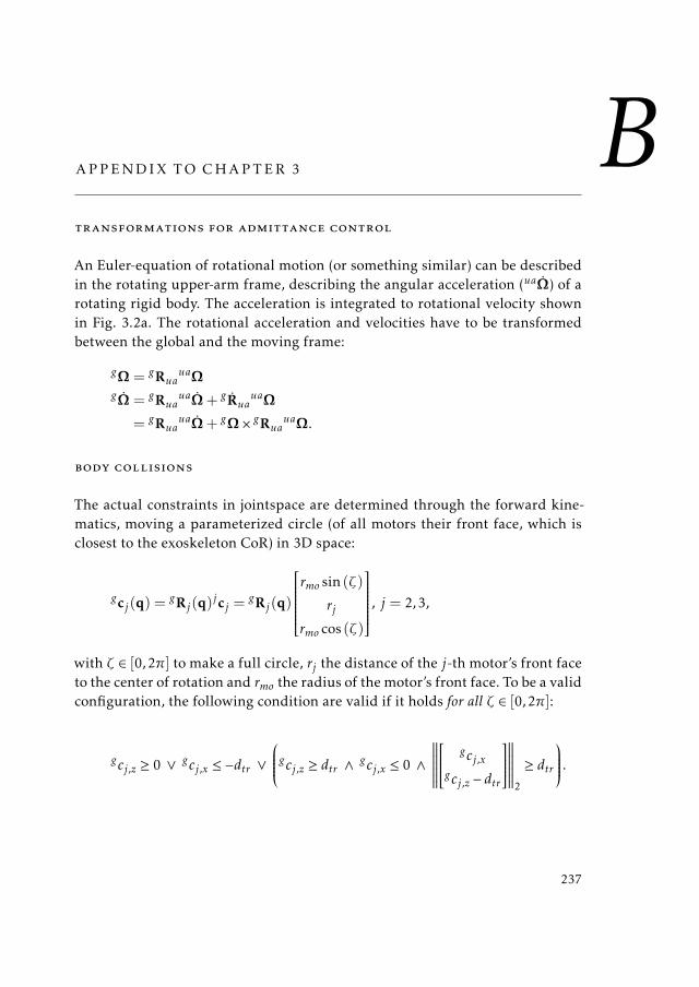
BAPPENDIX TO CHAPTER 3
transformations for admittance control
An Euler-equation of rotational motion (or something similar) can be described
in the rotating upper-arm frame, describing the angular acceleration (uaΩ) of a
rotating rigid body. The acceleration is integrated to rotational velocity shown
in Fig. 3.2a. The rotational acceleration and velocities have to be transformed
between the global and the moving frame:
gΩ = gRua
uaΩ
gΩ = gRua
uaΩ+ g Rua
uaΩ
= gRuauaΩ+ g
Ω × gRuauaΩ.
body collisions
The actual constraints in jointspace are determined through the forward kine-
matics, moving a parameterized circle (of all motors their front face, which is
closest to the exoskeleton CoR) in 3D space:
gcj (q) =gRj (q)
jcj =gRj (q)
rmo sin (ζ)
rj
rmo cos (ζ)
, j = 2,3,
with ζ ∈ [0,2π] to make a full circle, rj the distance of the j-th motor’s front face
to the center of rotation and rmo the radius of the motor’s front face. To be a valid
configuration, the following condition are valid if it holds for all ζ ∈ [0,2π]:
gcj ,z ≥ 0 ∨ gcj ,x ≤ −dtr ∨
gcj ,z ≥ dtr ∧ gcj ,x ≤ 0 ∧∥∥∥∥∥∥∥
gcj ,xgcj ,z − dtr
∥∥∥∥∥∥∥2
≥ dtr
.
237

238 appendix b
The first condition states that the motor is on the ‘right’ (positive in zg ) of the
global XY -plane. The second condition states that the motor is behind (negative
in xg ) the YZ-plane behind the back. The third condition states that the motor
is outside the quarter cylinder connecting both planes.
arm collisions
The constraint can be denoted as follows:
guua · gωj ≤ cos(αua,j ), j = 1,2,3.
The angles αua,j are found through the implicit equation:
rj sin (αua,j ) = rmo cos (αua,j ) + rua,
which can be solved through an imaginary detour, swapping the trigonometric
functions with their complex exponents, yielding:
αua,j = −i ln
√
r2mo + r2j − r2ua + irua
rj − irmo
, i =√−1, (B.1)
with ln (·) the natural logarithm. This equation yields a real solution for the
collision cone angle.
First, we check if the upper arm is between two motor axes. Where pj is the
normalized projection vector of uua on the plane generated by gωj andgωj+1.
gnj =gωj × gωj+1
‖gωj × gωj+1‖
gpj =gnj × (guua × gnj )
‖gnj × (guua × gnj )‖.
The sum of the two absolute angles between pj and the rotation axes has to be
more than the angle between both rotation axes (the arc φj ):
arccos(gpj · gωj ) + arccos(gpj · gωj+1) > φj , j = 1,2.

appendix b 239
If the above constraint does not hold, this is only problematic if the arm is close
enough to the plane formed by the rotation axes to hit the link. Therefore it
should hold that:
|gnj · guua| ≤ sin (αli,j ), j = 1,2,
where αli,j is found in a similar way as in (B.1), but by substituting rmo with
dli/2. Both motor and link collision conditions are kinematically only depen-
dent on φ1, φ2, q2 and q3.
conditioning
The sub-determinants of Jacobian J(q) are given by:
∆1 = det [gω1gω2
gω3]
∆2 = det [gω2gω3
gω4]
∆3 = det [gω1gω2
gω4]
∆4 = det [gω1gω3
gω4].
The condition for proper conditioning is then:
max([|∆1|, |∆2|, |∆3|, |∆4|]) ≥ η.
with η ≈ ‖Ω‖max‖qmax‖ , approximately the ratio between the shoulder and exoskeleton
velocities for minimum norm solutions.
algorithm limit cases
If T → 0 this algorithm reduces to a continuous time version, which removes the
distinction between qk−1 and q+k . If the gain K is high, the saturation will clip
the highest velocity to some predefined bound. This way, the convergence rate
can be increased up to when the exoskeleton moving as fast as possible along
Qns(q+k ). This is a valid, but more aggressive solution to the problem, giving
high joint speeds and accelerations.

240 appendix b
bounds on K
We recognize (3.25) to be a discrete Euler integrator with a gain K in a closed
loop. This process has a pole location at p = 1 − KT in the z-domain. For stable
convergence |p | < 1. This gives as a gain condition: 0 ≤ K < 2/T . To have non-
oscillating exponential convergence the upper bound on K is actually 1/T .
finding the nullspace-configuration set efficiently
In computer applications it is preferred to numerically integrate (3.15) in two
directions from q up to some point that the end-points (modulo 2π) meet (the
difference is smaller than 2 integration steps). Since the eigenvector uN acquired
through numerical algorithms can have ‘random’ sign, every discrete spatial in-
tegration instant κ (not to be confused with temporal integration of the motion
over time instant k) a direction correction is made through the inner product of
uN of the current (κ) and its values of the previous integration step (κ − 1):
uN ,κ,corr = uN ,κsgn(uN ,κ ·uN ,κ−1).
finding ξ 0
Eq. (3.22) is in computer applications calculated by finding a the minimal value
of δ (ξ ) in the array of all elements of the nullspace-configuration curve. Since
the spatial integration in (3.15) goes with unit-velocity, the array-index imin be-
longing to qmk is directly proportional to ξ with integration step ∆x. Therefore
ξmρ = imin∆xρ.
CAPPENDIX TO CHAPTER 4
derivation of transfer function
The full transfer function for the system shown in Figure 4.4 is given by
Ya =v
Fext
=Yr(HdSf (Gf +C ′Y ∗v ) + 1)
Yr(Zps +D) + 1,
with
D = Hd(CfbSvkr +Gf Sf Zps −C ′Y ∗vδZ )C ′ = Cfb +Cff
Y ∗v = Yvkr
δZ = SaZps − Sf Zps
Hd = HZOHHikr .
The disturbance force influence is given by
Sp =v
Fdist=
YrYr(Zps +D) + 1
.
241
242 appendix c
In its most elaborate form, the following subsystems are used
Yr =1
mrs+ br
Cfb = kp +kis+
kds
τds+ 1
Cff = µff s+ βff
Zps =mpss, Zps =µcs
τcs+ 1
HZOH =1− e−sTs
sTs, Hi = kT
e−sTd
τis+ 1
Yv =kas
2 + s
mvs2 + bvs+ kv
Sv =1
τvs+ 1, Sf =
1
τf s+ 1, Sa =
1
τas+ 1.
Here it is assumed Yr describes a stiff robot system.
derivations of stability and passivity
Naive feedback only (Sec. 4.5.3)
Combining Eqs. (4.3) to (4.6) yields apparent admittance
Ya =1
s
mvs2 +Kps+Ki
a2s2 + a1s+ a0,
with a2 = (mr+mps)mv , a1 = (Kp+br)mv+Kpmps, a0 = Ki(mv+mps), Kp = kpk2r
and Ki = kik2r .
Setting s = jω, we arrive at
Ya(jω) =(mvω
2 −Ki)− jKpω
a1ω2 + j (a2ω3 − a0ω)=
Na(jω)
Da(jω).

appendix c 243
The positive real condition becomes
RNaRDa+ INaIDa ≥ 0, ∀ωc1ω
4 + c2ω2 ≥ 0, ∀ω
c1 = (Kp + br)m2v −Kpmrmv
c2 = −Kibrmv
For passivity we require that c1 ≥ 0 and c2 ≥ 0. Dividing both conditions by mv
(under the constraint that mv > 0) gives passivity conditions (4.7) and (4.8).
Naive Accommodation Control (Sec. 4.5.4)
Combining Eqs. (4.3), (4.4) and (4.6) with Yv = 1/bv yields apparent dynamics
Ya =(Kp + bv)s+Ki
b2s2 + ((Kp + br)bv +Kimps)s+ bvKi
with b2 = (mr +mps)bv +Kpmps. Analogous to the method in the previous sec-
tion, we set s = jω and arrive at the positive real condition
d1ω2 + d2 ≥ 0, ∀ω
d1 = (Kp + bv)(Kp + br)bv −Kimrbv
d2 = bvK2i
For passivity we require that d1 ≥ 0 and d2 ≥ 0. Dividing d1 by bv (under the con-
straint that bv ≥ 0, which also conforms directly to d2) we arrive at the passivity
conditions mentioned in the main text.
Naive Stiffness Control (Sec. 4.5.4)
Analogous to the previous section, setting Yv =skv
yields apparent admittance
Ya =Krs
2 + (Ki + kv)s
Kpmpss3 + γ2s2 + (Kp + br)kvs+Kikv,

244 appendix c
with γ2 = (mr +mps)kv +Kimps. This system is always stable for positive choice
of parameters. Setting s = jω yields the positive real condition
e1ω4 + e2ω
2 ≥ 0, ∀ωe1 = Kpkvmr
e2 = (Kp + br)k2v +Kibrkv .
Since both e1 ≥ 0 and e2 ≥ 0 for positive parameters, this system is always pas-
sive.
Element combinations (Sec 4.5.5)
Combining different haptic elements into the virtual dynamics results in addi-
tions of passivity conditions. Therefore, we will derive the passivity conditions
for a mass-spring-damper system
Yv =s
mvs2 + bvs+ kv,
and show how it relates to the passivity conditions found in the preceding sec-
tions.
The apparent admittance for this system becomes
Ya =mvs
3 + (bv +Kp)s2 + (Ki + kv)s
mrmvs4 +φ3s3 +φ2s2 +φ1s+Kikv,
with φ3 = brmv + bvmr + Kpmv , φ2 = brbv + bvKp + Kimv + kvmr and φ1 =
bvKi + brkv + Kpkv . This system is not necessarily stable for positive choice of
parameters. The full stability condition (found by generating the Routh array)
is given as:
bv(br +Kp)([b2r +K2
p ]kvmv + [brbv + bvKp +Kimv ]Kimv+
[brbv + bvKp + kvmr ]kvmr + 2brKpkvmv + b2vKimr)
≥ 2(br +Kp)(bvKikvmrmv).
Note that the l.h.s. and the r.h.s. share a common factor of bv(br + Kp). This
complicated condition is effectively an upper bound on Ki .

appendix c 245
Analogous to the method in the previous sections, we set s = jω and arrive at
the positive real condition
λ1ω6+λ2ω
4 +λ3ω2 ≥ 0, ∀ω
λ1 =brm2v +Kpm
2v −Kpmrmv
λ2 =brb2v + bvK
2p + b2vKp + brbvKp − brKimv − bvKimr − 2brkvmv+
Kpkvmr − 2Kpkvmv
λ3 =bvK2i + brk
2v +Kpk
2v + brKikv .
Inspection of λ1 shows that it is the same as condition (4.7) (or c1 in the analysis
of the ‘Naive feedback only’). This shows that condition (4.7) is invariant to the
addition of other haptic elements. Inspection of λ3 shows that it is an addition
of conditions d2 and e2 from the analysis on Naive Accommodation and Naive
Stiffness control. Inspection of λ2 shows that it is a summation of d1, e1, c1 (i.e.
condition (4.8)) and an extra term δmk = −2(Kp + br)kvmv . This leads to all the
combinations discussed in Sec. 4.5.5 and shown in Table 4.2.
Guideline 1: Using feed-forward control
We set Yv = 1/mvs, and change the control force to
Fc = kr
(kps+ ki
s(vd − krv) + (µffs+ βff)vd +Gf Fext
)
.
The apparent admittance becomes
Ya =1
s
(µffk2r + (1+Gf kr)mv)s
2 + (βffk2r +Kp)s+Ki
f2s2 + f1s+ f0s,
with f2 = µffk2r mps + (mr + mps)mv , f1 = (Kp + br)mv + (βffk
2r + Kp)mps and
f0 = (mv+mps)Ki . This system is always stable for positive choice of parameters.
Setting s = jω yields the positive real condition
g1ω4 + g2ω
2 ≥ 0, ∀ωg1 = (Gf kr + 1)(Kp + br)m
2v − (Kp + βffk
2r )mrmv + (Kp + br)µffk
2r mv
g2 = (βffk2r − br)Ki .

246 appendix c
For passivity we require that g1 ≥ 0 and g2 ≥ 0. Dividing g1 by mv we arrive
at the passivity conditions of Eqs. (4.9) and (4.10). Looking at condition g1 ≥ 0,
it can be noted that feed-forward control of the mass reduces the robot inertia
from the view of the feedback controller.
Guideline 2: Avoid force filtering
We apply a first-order low-pass filter to the measured force
Sf =1
τf s+ 1.
This makes the virtual dynamics effectively
Y ′v = YvSf =1
mvs
1
τf s+ 1=
1
τf mvs2 +mvs.
We set ki = 0, since we know that the naive admittance controller has that re-
quirement for being positive real, and adding a low pass filter will make it worse.
The apparent admittance becomes
Ya =1
s
mvτf s2 +mvs+Kp
h2s2 + h1s+ (Kp + br)mv +Kpmps,
with h2 = (mr + mps)τf mv and h1 = ((Kp + br)τf + mr + mps)mv . This gives
positive real condition
n1ω4 + n2ω
2 ≥ 0, ∀ωn1 = (Kp + br)m
2vτ
2f
n2 = (Kp + br)m2v −Kpmv(mr + (Kp + br)τf ).
For passivity we require that n1 ≥ 0 and n2 ≥ 0. Which results in the passivity
condition in (4.11).
Passive physical equivalence of filtered dynamics:
Note that first and second order filters change accommodation and stiffness con-
trol into admittance control effectively. Consider pure spring virtual dynamics

appendix c 247
Yv(s) = s/kv in series with a second order low-pass filter B2(s) (with cut-off
frequency ωc = 1/τc and relative damping ζ):
Yv(s)B2(s) =s
kv
1
τ2c s2 + 2ζτcs+ 1=
s
m′vs2 + b′vs+ kv,
which is a typical mass-spring-damper admittance form with apparent virtual
inertia m′v = τ2c kv and virtual damping b′v = 2ζτckv .
Similarly, for accommodation control, a first order low-pass filter on the mea-
sured force will turn the dynamics into admittance control. Consider pure damp-
ing virtual dynamics Yv(s) = 1/bv in series with a first order low-pass filter
B1(s) (time constant τc):
Yv(s)B1(s) =1
bv
1
τcs+ 1=
1
m′vs+ bv,
which is a typical mass-damper admittance form with apparent virtual inertia
m′v = τcbv . The same holds true for virtual dynamics of spring-damper form
with a first order low-pass filter in series.
Guideline 3: compensate post-sensor inertia
We generate an additional force reading to counteract the post-sensor effects
SaZpss =µcs
τcs+ 1v.
We set ki = 0, since it will interfere with passivity, because we are not changing
the inner velocity loop (this assumption was validated). The apparent admit-
tance becomes
Ya =1
s
(mvτc)s2 + (Kpτc +mv)s+Kp
(mr +mps)mvτcs2 + q1s+ q2,
with q1 = ((Kp+br)τc+mr+mps)mv+Kpmpsτc and q2 = (Kp+br)mv+Kp(mps−µc). For uncoupled stability we require q2 ≥ 0, which puts an upper bound on
the maximum value for µc.

248 appendix c
The positive real condition becomes
r1ω4 + r2ω
2 ≥ 0, ∀ωr1 = (Kpmv −Kpmr + brmv)τ
2c mv
r2 = (Kp + br)m2v −Kpmv(mr + µc)−K2
pµcτc.
For passivity we therefore require that r1 ≥ 0 and r2 ≥ 0. Condition r1 equals the
condition in (4.7). Condition r2 is an additional constraint. The total condition
is
mv ≥Kp
Kp + br(mr + µc) +
K2p
Kp + br
µcmv
τc.
If τc → 0, the last part on the right hand side of the equation drops and we end
up with the condition discussed in the text.
Guideline 4: use some virtual damping
The virtual dynamics has an additional damping parameter bv
Yv =1
mvs+ bv.
The apparent admittance becomes
Ya =mvs
2 + (Kp + bv)s+Ki
(mr +mps)mvs3 + t2s2 + t1s+Kibr,
with t2 = (mr +mps)(Kp + bv) + brmv and t1 = (mv +mps)Ki + (Kp + br)bv .
Uncoupled stability of this system is guaranteed if all parameters are positive,
since stability condition t2t1 ≥ (mr +mps)mvKibr always holds in that case.
If we set s = jω, the positive real condition is found to be
u1ω4 + u2ω2 + u3 ≥ 0, ∀ω
u1 = (Kpmv −Kpmr + brmv)mv
u2 = bv(Kp + bv)(Kp + br)− ki(brmv + bvmr)
u3 = Kibv .

appendix c 249
Therefore, for strict passivity we require that u1 ≥ 0, u2 ≥ 0 and u3 ≥ 0. These
conditions are discussed in the text. Discriminant analysis would yield too com-
plicated conditions for passivity.
Guideline 5: modify the velocity reference
Although the virtual dynamics is described by a pure inertia, the effective vir-
tual dynamics has the form
Y ′v =kas+ 1
mvs.
The apparent admittance becomes
Ya =1
s
(Kpka +mv)s2 + (Kp +Kika)s+Ki
v2s2 + v1s+ (mv +mps)Ki,
with v2 =mrmv +mps(mv +Kpka) and v1 = (Kp + br)mv + (Kp +Kika)mps.
The positive re condition:
w1ω4 +w2ω
2 ≥ 0, ∀ωw1 = (Kp + br)m
2v + ((K2
p + brKp −Kimr)ka − kpmr)mv
w2 = (kaKi − br)Kimv .
Therefore, for passivity we require that w1 ≥ 0 and w2 ≥ 0.
Guideline 6: increase velocity loop bandwidth
Apparent Admittance:
Ya =1
s
mvτds3 + x′2s
2 + (Kp +Kiτd)s+Ki
(mr +mps)mvτds3 + x2s2 + x1s+ x0,
with x′2 =mv +Kd +Kpτd , x2 = (mr +mps)mv +(mv +mps)Kd +((Kp + br)mv +
Kpmps)τd , x1 = (Kp + br)mv +Kpmps +Kiτd(mv +mps) and x0 = (mv +mps)Ki .
For stability we demand that (derived from the Routh array):
x2x1 ≥ (mr +mps)mvx0

250 appendix c
which always holds for positive parameters.
The positive real condition yields
y1ω6 + y2ω
4 + y3ω2 ≥ 0, ∀ω
y1 = (Kd + (Kp + br)τd)τdm2v − (Kpτd +Kd)mrmvτd
y2 = (Kp + br)m2v + (br(Kd −Kiτ
2d )−Kpmr)mv
y3 = −brKimv .
Therefore, for passivity we require that all parameters are positive, and that
y1 ≥ 0, y2 ≥ 0 and y3 ≥ 0. Using this system with non-zero positive integral
gain cannot result in a passive system. The other two passivity conditions are
discussed in the text in Sec. 4.6.6.
system with internal compliance transfer function and positive
real conditions
The equations of motion for the system in Fig. 4.14 are given by
(mrγ′s+ br)v
′ =Fc + krFd + (v − v′)(ks/s+ bs)
mrγsv =Fext −mpsvs − (v − v′)(ks/s+ bs).
The equations for Yv , vd stay the same as in Eqs. (4.4) and (4.5). Eq. (4.6) changes
slightly to
Fc = krkps+ ki
s(vd − krv′)
The apparent admittance (felt at the distal mass) is given by
Ya =v
Fext=
1
s
z′4s4 + z′3s
3 + z′2s2 + z′1s+ z′0
z4s4 + z3s3 + z2s2 + z1s+ z0,

appendix c 251
with numerator coefficients
z′4 =mrmv(1−γ)z′3 = (Kp + br + bs)mv
z′2 = (Ki + ks)mv + bskpkr
z′1 = bskikr + kpkrks
z′0 = kikrks.
Denominator coefficients are given by
z4 =mvm2r (γ −γ2) +mpsmvmr(1−γ)
z3 = ((Kp + br + bs)mps + bsmr + (Kp + br)γmr)mv
z2 = (brbs + (Ki + ks)mps + ksmr + bsKp + γKimr)mv + bskpkrmps
z1 = ((Kp + br)ks + bsKi)mv + (bski + kpks)krmps
z0 = Kiksmv + kiksmpskr .
Because the denominator polynomial is of fourth order, there are two non-trivial
conditions to achieve marginal uncoupled stability
z3z2 − z4z1 = Γ1 ≥ 0
Γ1z1 − z23z0 ≥ 0.
These conditions are not insightful and we assume the controller is stable. Sta-
bility depends mostly on integral gain ki and internal stiffness ks.
Setting s = jω we arrive at the positive real condition
ξ1ω8 + ξ2ω
6 + ξ3ω4 + ξ4ω
2 ≥ 0, ∀ω

252 appendix c
with
ξ1 = (γ2 − 2γ + 1)bsm2rm
2v
ξ2 = (−bski − kpks)m2r krγ
2 + (kskpmr + (2mvkr +mr)bski−bskp(Kp + br))mrkrγ +mvbs((Kp + br)(Kp + br + bs)−2Kimr)−mrb
2s kpkr
ξ3 = ((brks − bsKi)mrkikrγ + (bsK2i + (Kp + br)k
2s )mv−
(brb2s ki + kpmrk
2s )kr)mv
ξ4 = −brkikrk2s mv .
For passivity we therefore require that ξn ≥ 0, n = 1, 2, 3 and 4. From these
conditions it becomes hard to determine what constitutes a passive design. Only
from ξ1 it is required that γ ≥ 0. Condition ξ4 is the same as (4.8), stating that
no integral velocity gain can be used to remain passive.

DAPPENDIX TO CHAPTER 5
a counter-example to the method of nabeel et al.
Consider Fig. 5.2, a robot with mass mr = 1 kg and drive train damping of
br = 0.1 Ns/m. It is admittance controlled to behave like a virtual mass of
mv = 0.5 kg by a position controller with feedback gain kp = 250 N/m. The
admittance controlled device interacts with a spring-like environment given by
impedance Ze(s) = ke/s, with environment stiffness ke = 1000 N/m. See the fol-
lowing subsection for the equations of motion and the transfer function for the
admittance controlled system*. The admittance of the admittance controlled sys-
tem is given by Ya. The closed loop behavior of the admittance controlled system
interacting with the spring-like environment is given by vr/Fh = Ya/(1+YaZe).
An external force Fh of 1 N acts for 0.001 s on the system to perturb the sys-
tem from the origin. Fig. D.1 shows the robot velocity, ingoing (Ein) and out-
going (Eout) energy according to the definitions of Nabeel et al. [146] and the
exchanged energy between the admittance controlled device and a human (Ehr).
These energies are calculated as follows by their time derivative:
Ein(t) =
Fh(t)vd(t), if Fh(t)vd(t) > 0
0, otherwise
Eout(t) =
Fc(t)vd(t), if Fc(t)vd(t) > 0
0, otherwise
Ehr(t) = Fh(t)vr(t)
Nabeel et al. claim that it is sufficient to enforce Eout(t) to be smaller than, or
equal to, Ein(t) for the system to be passive at the interaction port Ihr. This ex-ample shows in Fig. D.1 a counter-example where this condition almost always
holds (i.e. Eout(t) < Ein(t) almost always), but the system is unstable (the veloci-
*Note that for this example α = 1m β = 0, γ = 1, kd = 0 Ns/m.
253

254 appendix d
0 0.2 0.4 0.6 0.8 1−0.5
0
0.5
1
Velocity
[m/s]
Robot and Model Velocity
Model Vel. Robot Vel.
0 0.2 0.4 0.6 0.8 110−10
10−6
10−2
Energy[J]
Ingoing and Outgoing Energy
Ein Eout
0 0.2 0.4 0.6 0.8 1−80
−60
−40
−20
0
Energy[m
J]
Exchanged Human-Robot Energy
Ehr
Figure D.1: Top) robot and virtual model velocities. Note that they both show an unsta-ble growing behavior due to the initial system perturbation. Middle) The in-going and outgoing energies according to Nabeel et al. [146] (see text). Notethat Eout(t) is almost always smaller than Ein(t). According to Nabeel et al.this system should be passive at the human-robot interface. Bottom) The en-ergy exchanged at the human-robot interface. Since the energy is negativeand becomes more negative over time, it shows that this system is not pas-sive at the human-robot interface.

appendix d 255
ties and positions keep growing) and not passive (i.e. active) at the man-machine
interface, because Ehr(t) is only negative and becomes more negative over time.
prc for a parameterized naive admittance controller
Consider Fig. 5.5. The equation of motion for the robot system (in the Laplace
domain) is given as:
mrsvr + brvr −(
kd +kp
s
)
(vd − vr) = αFh.
The equation of motion for the virtual dynamics used in the admittance con-
troller:
mvsvd + β
(
kd +kp
s
)
(vd − vr) = γFh.
This gives a total transfer function for the apparent admittance of the con-
trolled system:
vrFh
=αmvs
2 + kd(αβ+ γ)s+ kp(αβ+ γ)
mrmvs3 + ((br + kd)mv + βkdmr)s2 + (kpmv + β(brkd + kpmr)s+ βbrkp.
By setting s = jω, we arrive at the PRC given in the text (see Chapter 4 and
Appendix C on how to calculate the PRC polynomial)
a2ω4 + a1ω
2 + a0 ≥ 0, ∀ωa2 =mv(αmv(br + kd)−γkdmr)
a1 = br(k2dβ(αβ+ γ)− kpmv(2αβ+ γ))
a0 = βbrk2p (αβ+ γ).
energy bookkeeping
The continuous-time controller needs to be time quantized with sample time T
following the convention shown in Fig. D.2. The new time index variable used
for discrete time is k. Due to discretization and non-zero finite calculation times,
the control force from the motion controller will be effectively output with one
sample time delay (see the Fig. D.2 caption for an explanation).

256 appendix d
k − 1 k k+ 1
u(k − 1) u(k) u(k+ 1)w(k − 1) w(k) w(k+ 1)
time→
k k+ 1
tc (k − 1) tc (k)
Figure D.2: Signals u or calculated variablesw are sampled and calculated respectively atsample instances k ∈Z
+. The time leading up to sample instant k is denoted
as sample k. Calculating w(k) actually takes variable non-zero time tc(k). Itwill take this time duration after the sample instant k for values or signals tobe available for output. For proper system determinism, signals calculatedduring tc(k) are output later at sample instant k+ 1.
The virtual dynamics with semi-implicit Euler integration become
vd(k+ 1) = vd(k)−Tβ(k)
mvvd(k) + T
Fh(k)
mv
xd(k+ 1) = xd(k) + Tvd(k+ 1).
Here β(k) is the variable damper that makes the system SPIS.
For discrete time systems (5.1) can be rewritten as a sum of integrals over all
samples (assuming t to be an integer multiple of sample time T )
E(t) =t/T∑
k=1
(∫ Tk
T (k−1)F(τ)v(τ)dτ
)
=t/T∑
k=1
∆E(k)
At a power port of impedance causality only, motion is imposed on the device
(v(t)) while the force applied (e.g. by the actuator) is assumed to be constant
during a sampling interval F(k). This gives
∆E(k) = F(kT )
∫ Tk
T (k−1)v(τ)dτ
= F(kT )[x(Tk)− x(T (k − 1))]
which is an exact discrete energy bookkeeping, since the device position x(t)
can be exactly retrieved. Energy exchanged with the virtual dynamics behaves
in the same way: a constant force on the model generates a state transition with

appendix d 257
position difference x(k)− x(k −1). Therefore, the bookkeeping of virtual energy
exchanged from the human to the virtual model is given by
∆Ehv(k) = Fh(k − 1)[xd(k)− xd(k − 1)]Ehv(k) = Ehv(k − 1) +∆Ehv(k)
The kinetic energy stored in the virtual system is given by
Hv(ξ) =1
2mvv
2d (k).
Neither F(t) nor v(t) is constant at the Ihr power port of the system. There-
fore, the energy exchanged between the human operator and the device can-
not be exactly determined. The energy need not be tracked accurately for this
method to work. Therefore, the assumption that the input signals from the en-
vironment are of a bandwidth lower than the Nyquist frequency of the system
is sufficient to get a good approximation of the real exchanged energy between
the human and robot Ehr(k).


ACKNOWLEDGMENTS
The work presented in this dissertation would not have been possible without
the help, supervision, moments of fun, moments of frustration, andmental stim-
ulation provided by family, friends and colleagues.
First of all, I would like to thank Arno Stienen for initiating the H-Haptics
project’s work package at the UT. Your ideas on the subject have guided most of
my research. Your supervision has helpedme tremendously; especially with gen-
erating potential ideas and helping me with scientific writing. I feel that your
interest in directly useful applications, and my interest in more fundamental
problems and modeling complemented each other well. Assisting you in what
is nowadays called the ‘Biorobotics minor’, which you initiated in 2013, has been
an interesting and rewarding experience. Second, I would like to thank my sec-
ond supervisor and promotor Herman v.d. Kooij. Without you I would literally
not have been able to finish my PhD. Your input for my paper on admittance
control has been very valuable. Your flexibility during the time I was finishing
the work is highly appreciated. Motivated by you and Arno, I have had the expe-
rience of teaching quite a few lectures in several courses: Control Engineering
for BMT-M9 (2013, now Biorobotics), Biomechatronics, and Human Movement
Control. This process helped me appreciate the transfer of knowledge to a new
generation of students in such a way that I would like to spend part of my future
academic career teaching. Third, I would like to thank the rest of my graduation
committee; Stefano Stramigioli, Anton Stoorvogel, Andre de Boer, Etienne Bur-
det and David Abbink for taking the time and effort to read and comment on
my work.
From my H-Haptics work package I thank Jack Schorsch, my PhD comrade
from TU Delft. Collaboration proved to be a bit harder than initially expected,
due to diverging research lines. The discussion on robocentric versus anthro-
pocentric lifting of heavy weights has not been fully settled yet, at least not for
me! We should definitely revisit that topic in the (near) future. We will, without
a doubt, collaborate soon anyway because of your newly developed drive trans-
mission. Freek Tonis from Hankamp Gears and Hankamp Rehab, I thank you
for your seemingly infinite patience with the project. I want to thank you for
all your time, contributions and ideas. I especially want to mention your flex-
259

260 acknowledgments
ibility concerning the myriad of students that have visited Hankamp to work
in some way for the project. At the end of the project we have now ‘an idea’ of
what the stronger MAS can do. Let us develop this idea further in the near fu-
ture. This also leads me to Koen Heuver and Michel van Hirtum, who have been
indispensable in designing the automated version of the MAS system. Further-
more, I thank Ruud de Nooij and Linda van den Bedem form Siza and Giuseppe
Radaelli and Boudewijn Wisse from Intespring/Laevo for being involved in the
project and giving useful user feedback.
Although I thank all other H-Haptics participants and colleagues, I explic-
itly want to mention David Abbink and Frans v.d. Helm who both oversaw the
complete H-Haptics consortium. A special shout-out to Femke van Beek, Jeroen
Wildenbeest andDebjyoti Bera for the interesting and stimulating autumn-school
week in 2013. It really taught me a lot about human factors research. I also
want to mention Irene Kuling, for visiting in 2015 when I was still in Chicago
and for an interesting Eurohaptics conference (together with Femke, Erik and
Jos) in London in 2016. Piet Lammertse, the admittance control guru from FC-
S/Moog, I thank for sharing his thoughts and insights on the control method.
Jeroen Smeets from the VU I thank for helping us in setting up the Fitts’ Law
and damping fields research and assisting with obtaining ethical approval for
those experiments.
Next, I want to move on to my colleagues at the Biomechanical Engineering
group at the University of Twente. I would like to thank Bart Koopman for being
my boss. Although we have not discussedmuch about work, my interaction with
you through collaboration with Joan has been very useful, leading to several
publications together. Next, I want to thank Martijn Wessels for collaborating
in the 4-DOF shoulder exoskeleton research. I still hope that a full size version
of your initial design will one day be produced. I want to thank Edsko Hekman
for helping me supervise some of my MSc students in mechnical design ori-
ented assignments. I also thank you for useful input about mechanical design
in general. Edwin van Asseldonk I thank for teaching me Human Movement
Control and explaining about human factors research. Lianne Bode-Bode and
Jeanine Lodeweges-De Vries, I thank you both for being the effective group lead-
ers behind the screens. Without your help and your infinite knowledge about
the university’s bureaucracy, nothing would ever get done!
Ravi Sinha and Gijs van Oort I thank for being my first office mates when I
started in 2012. Gijs, I also thank you for your thoughts and insights for the
4-DOF shoulder exoskeleton work we did. Many thanks to Joan Lobo Prat. We

acknowledgments 261
shared hundreds of rides on the Syntus train between Zutphen and Enschede,
discussing many interesting, practical, fundamental and future possibilities of
interaction control and intention detection for assistive devices. The trips by
train have now become quite dull after you finished your PhD and moved to the
USA. I am also honored you picked me to be one of your paranymphs. I think
we all remember how smoothly that went during the ceremony (. . . not very)! I
want to thank Serdar Ates for being a constant source of positivity, even when al-
ways working very hard on the Script project’s deadlines. We have shared many
moments of fun, drank good beer, had good food and exchanged quite a few
inappropriate remarks! This, except for the inappropriate remarks, also holds
for Israel Mora Moreno. Although you did not spend a lot of time with the
group, I thank you for joining Joan, Serdar and me on many occasions. Next,
I want to thank Kostas Nizamis. As Joan’s ‘protege’ you have risen to become
an indispensable member of the group. I like how you are always ready and
available to help people. I envy your teaching and presentation skills. You are
possibly the most easy-going and chill person to be around and I am very happy
that you wanted to be my paranymph. This leads me to my second paranymph:
Niek Beckers. I like how we are interested in similar questions regarding human
movement control, and how we have managed to incorporates some of this in
the Biomechatronics and Human Movement Control Courses. You are a great
guy. I thank you for helping me a lot giving input to my work and proofread-
ing several of the chapters in my thesis. My long-time office mate Victor Sluiter
is the go-to-guy that knows everything. Your critical view on what we do in
the group is extremely useful. The two of us helping students extensively with
building and programming their robots in the BMT-M9 projects in 2013 and
2014 is a great memory. Stergios Verros, I thank you for being such a nice guy
that is always willing to help. I like how you continue Joan and my ideas for
interaction control for the trunk. Jos Meuleman, although you have now been
gone a while, I thank you for helping me get started with the whole ‘admittance
control thing’, especially together with Erik and Ralph. It was a pleasant sur-
prise, meeting again at the Eurohaptics conference in 2016. I have had some
great times with Alex Kuck. Thank you for visiting me in Chicago, where we
met some. . . interesting people. We share a lot of the same ideas and wishes for
the world and the scientific community. I hope you will be come back to En-
schede, or at least the Netherlands, to collaborate academically or in our own
projects. I thank Carsten Voort for helping me with setting up the first setup for
the Biomechatronics Haptics practical. Furthermore, I like our continued col-

262 acknowledgments
laboration into interaction control between our group and your company. I also
thank Geert Folkertsma from the Robotics and Mechatronics (RaM) group. We
were colleagues at RaM briefly, but we go way back to the first year of the uni-
versity’s Honors Program. It was too bad that, in the limited time left, we were
not able to incorporate your energy based control ideas into admittance control
that easily. However, collaboration between us and our groups will ensure that
this will happen soon!
I also thank the Surgical Robotics guys Guus Vrooijink, Federico Ongaro and
Klaas Jelmer Boskma from Groningen for the fun time in Singapore during
Biorob 2016. And, of course, I thank the other members of the group that were
also there during (part of) my PhD who contributed to making the working day
more bearable; (in random, but somewhat chronological, order) Youri van Veen,
Jan de Jong, Bas Behrens, Wouter Abbas, Letian Wang, Bram Koopman, Gerdine
Meijer, Ard Westerveld, Rene Fluit, Vincenzo Carbone, Iris Hoogendoorn, Thijs
Lohuis, Daphne Boere-van Baal, Antoon Philippi, Bob Giesberts (also for help-
ing with the thesis cover!), Claudia Haarman, Hielke Kiewiet, Floor Kampfens,
Denise Engelhart, Tjitske Boonstra, Mark Vlutters, Amber Emmens, Heidi Wit-
teveen, Teun Stortelder, Martijn Grootens, Kyrian Staman, Quint Meinders and
everyone else that I forgot to mention!
Duringmy sabbatical at the Physical Therapy andHumanMovement Sciences
at Northwestern University in Chicago I had the opportunity to work with sev-
eral amazing people. I would like to explicitly thank Jules Dewald and Ana
Maria Acosta for the possibility to spend six months at the lab to work on the
NACT3D robot. I appreciate your trust in my work and our continuing collab-
oration. I thank Netta Gurari for sharing her insights and comments on some
of my work. I look back very positively on the more colloquial and practical
collaboration with Stuart Traxel and Paul Krueger working on the robot.
Next, I would like to thank all the Bachelor’s students, Master’s students and
interns that I have enjoyed supervising during (or even after, if the work wasn’t
finished. . . ) my time as a PhD candidate. I hope you learned as much from
me as I learned from you; Maarten Pijper, Ralph Macke (twice), Erik Euving
(twice), Floris Bloembergen, Nienke Schimmel, Koen Heuver, Anke Nesselaar,
Jose Alves, Barbara Cardoso, Dave Vogel, Dennis Niehoff, Nienke Bink, Robert
Roos, Stefan van Leuveren, Alexander Roosendaal, Martijn Schuurman, Harm
den Dekker, Rik Fierkens and Joeri Landman (twice). Tom Lankhorst, although
you have never been my student directly you have been more of a colleague. The
DISC summer-school in 2016 was more enjoyable with your and Erik’s presence.

acknowledgments 263
I want to explicitly mention the contributions of the following students; Floris,
thank you for visualizing Arno’s and my initial idea of the shoulder ROM vi-
sualization discussed in Chapter 2. Robert, thank you for getting the 4-DOF
shoulder test-setup to work. It was used for results in Chapter 3, and thanks to
your help with the setup that chapter will be published in IEEE-TNSRE. I thank,
Ralph and Erik for being my first BSc students whom I supervised together with
Jos. You helped me with my initial investigations into fundamental issues with
admittance control. Our collaboration has lead me to write Chapter 4, which
will be published in the IJRR. Joeri and Erik (again) I would like to thank for
their preliminary work into possible time-domain passivity enforcement for ad-
mittance control that leadme to write Chapter 5. Finally, Rik Fierkens has been a
tremendous help in performing experiments, and discussing about optimal con-
trol models. Your work contributes to the ideas presented in Chapters 6 and 7.
Finally, I want to acknowledge the contributions of Michel van Hirtum again; I
am very glad you managed to take over all of the design responsibilities for the
project at Hankamp. I thank you for all you have done and I congratulate you
on receiving your PDEng degree within our project.
I thank all my non work-related friends for our meet-ups and vacation trips.
I would like to explicitly mention Sil Nieuwhof; you also know what it is like
to climb this hill called ‘getting-your-PhD’. We should get back into the music
very, very soon!
My penultimate thanks are to my family.Mijn ouders, Carla and Leo. Ik bedank
jullie dat jullie dit voor mij mogelijk hebben gemaakt. Jullie morele steun en interesse
in mijn bezigheden zijn voor mij de hoofdredenen geweest om dit werk te doen en
het te blijven voortzetten. Mijn zus, Cynthia, bedank ik voor het zijn van mijn grote
voorbeeld tijdens mijn formatieve jaren. Mijn nichtje Quinte en neefje Jesse, die je
samen met Niek aan deze wereld hebt geschonken, zijn een onuitputtelijke bron van
plezier en inspiratie.
Finally, I would like to thank Anne.Anne, samen over de wereld en door het leven
reizen is een geweldige evaring. Bedankt voor het achter me staan tijdens betere en
slechtere dagen van mijn promotietijdperk. Jij, als maatje, aan mijn zijde gedurende
de afgelopen zeven en een half jaar is hetgeen dat dit alles betekenis en waarde geeft.
Ik hou van je.
Arvid Keemink
Zutphen, September 2017


B IOGRAPHY
Arvid Quintijn Leon Keemink was born
December 22nd, 1987, in Purmerend (the
Netherlands). He got his bilingual high
school degree (bilingual Atheneum) and In-
ternational Baccalaureate English A2 in 2005
at the Marnix College in Ede. He studied
Advanced Technology for his Bachelor’s de-
gree at the University of Twente, with a
minor in Aeronautical Engineering. He fol-
lowed the honors program at the University
of Twente from 2007–2009 and was one of
the co-founders and secretary of the honors
program student association H.V. Ockham.
During is Master’s degree in Mechatronics
at the University of Twente, he spent four
months at the ETH in Zurich (Switzerland) in
2010/2011 at the Autonomous Systems Lab-
oratory. He received his Master’s degree, cum laude, at the Robotics and Mecha-
tronics group at the University of Twente. He won the prize for best MSc thesis
at the faculty of EEMCS (Electrical Engineering, Mathematics and Computer
Science) for the academic year 2011/2012.
At the beginning of 2012 he started his PhD in Biomechatronics at the Biome-
chanical Engineering department at the University of Twente, under supervi-
sion of prof. dr. ir. Herman van der Kooij and dr. ir. Arno H.A. Stienen. He
was also involved in teaching control engineering and supervised seven BSc stu-
dents, seven MSc students and five interns during the course of his PhD.
During his PhD he spent six months abroad at the Physical Therapy and Hu-
man Movement Sciences department at Northwestern University in Chicago
(Illinois, USA) to implement admittance control on a custom robot to evaluate
human motor control after stroke.
He is currently investigating human-in-the-loop and self-learning optimiz-
ing controllers based on models of neuromuscular reflexes in humans to enable
spinal-cord-injury patients to walk with lower-extremity exoskeletons.
265


PUBL ICAT IONS
journal publications:
7. A.Q.L. Keemink, H. v.d. Kooij and A.H.A. Stienen, “Admittance Control
for Physical Human Machine Interaction”, accepted for publication in the
International Journal of Robotics Research.
6. A.Q.L. Keemink, G. van Oort, M. Wessels and A.H. A. Stienen, “Differen-
tial Inverse Kinematics of a Redundant 4R Exoskeleton Shoulder Joint”,
accepted for publication in IEEE Transactions on Neural Systems and Re-
habilitation Engineering.
5. J. Lobo-Prat, K. Nizamis, M.M. Janssen, A.Q.L. Keemink, P.H. Veltink,
H.F.J.M. Koopman and A.H.A. Stienen “Comparison between sEMG and
force as control interfaces to support planar armmovements in adults with
Duchenne: a feasibility study”, Journal of NeuroEngineering and Rehabil-
itation, vol. 14, no. 1, p. 73, 2017.
4. J.F. Schorsch, A. Q. L. Keemink, A.H.A. Stienen, F.C.T. van der Helm,
and D.A. Abbink, The Influence of Human-Robot Interaction Order Dur-
ing Fast Lifting Tasks for Different Levels of Weight Compensation, IEEE
Transactions on Human Machine Systems, accepted for publication Octo-
ber 2016.
3. J. Lobo-Prat,A.Q.L. Keemink, A.H.A. Stienen, A.C. Schouten, P.H. Veltink,
and H.F.J.M. Koopman, “Evaluation of EMG, force and joystick as control
interfaces for active arm supports”, Journal of NeuroEngineering and Re-
habilitation, vol. 11, no. 1, p. 68, 2014.
2. J.F. Schorsch, A.Q.L. Keemink, A.H.A. Stienen, F.C.T. van der Helm and
D.A. Abbink, “A novel self-aligning mechanism to decouple force and
torques for a planar exoskeleton joint”, Mechanical Sciences, vol. 2, no.
5, 2014.
1. M. Fumagalli, R. Naldi, A. Macchelli, F. Forte, A.Q.L. Keemink, S. Strami-
gioli, R. Carloni, and L. Marconi, “Developing an Aerial Manipulator Pro-
267

268 publications
totype: Physical Interaction with the Environment”, IEEE Robotics & Au-
tomation Magazine, vol. 21 , no. 3, p. 41, 2014
international peer-reviewed conference publications:
11. R.J.L. Macke, A.Q.L. Keemink and A.H.A. Stienen, “Passive Lower Back
Moment Support in aWearable Lifting Aid: Counterweight Versus Springs”,
Wearable Robotics: Challenges and Trends, 2016.
10. H.A. den Dekker, N.W.M. Beckers, A.Q.L. Keemink, H. van der Kooij
and A.H.A. Stienen, “Assessing the Usability of Remote Control Servos for
Admittance-ControlledHaptic FingerManipulators”, IEEE/RAS-EMBS In-
ternational Conference on Biomedical Robotics and Biomechatronics (Bio-
Rob), 2016.
9. A.Q.L. Keemink†, R.I.K. Fierkens†, J. Lobo-Prat, J.S.F. Schorsch, D.A. Ab-
bink, J.B.J. Smeets and A.H.A. Stienen, “Using Position Dependent Damp-
ing Forces around Reaching Targets for Transporting Heavy Objects: A
Fitts’ Law Approach”, IEEE/RAS-EMBS International Conference on Bio-
medical Robotics and Biomechatronics (BioRob), 2016.
8. P.N. Kooren, J. Lobo-Prat, A.Q.L. Keemink, M.M. Janssen, M.I. Paalman,
A.H.A. Stienen and H.F.J.M. Koopman, “Design and Control of the Active
A-Gear: a Wearable 5 DOF Arm Exoskeleton for Adults with Duchenne
Muscular Dystrophy”, IEEE/RAS-EMBS International Conference on Bio-
medical Robotics and Biomechatronics (BioRob), 2016.
7. A.H.A. Stienen† and A.Q.L. Keemink†, “Visualization of Shoulder Range
of Motion for Clinical Diagnostics and Device Development”, IEEE/RAS-
EMBS International Conference on Rehabilitation Robotics (ICORR), 2015.
6. J. Lobo-Prat, A.Q.L. Keemink, H.F.J.M. Koopman, A.H.A. Stienen and P.H.
Veltink, “Adaptive Gravity and Joint Stiffness Compensation Methods for
Force-Controlled Arm Supports”, IEEE/RAS-EMBS International Confer-
ence on Rehabilitation Robotics (ICORR), 2015.
5. K. Nizamis, J. Lobo-Prat,A.Q.L. Keemink, R. Carloni, A.H.A. Stienen, and
H.F.J.M. Koopman, “Switching proportional EMG control of a 3D end-
point arm support for people with duchenne muscular dystrophy”, IEEE/
†Indicates equal contribution.

publications 269
RAS-EMBS International Conference on Rehabilitation Robotics (ICORR),
2015.
4. J. Lobo-Prat, P.N. Kooren, A.Q.L. Keemink, M.I. Paalman, E.E.G. Hekman,
P.H. Veltink, A.H.A. Stienen, and H.F.J.M. Koopman, “Design and con-
trol of an experimental active elbow support for adult Duchenne Mus-
cular Dystrophy patients”, IEEE/RAS-EMBS International Conference on
Biomedical Robotics and Biomechatronics (BioRob), 2014.
3. J.F. Schorsch, A.Q.L. Keemink, A.H.A. Stienen, F.C.T. van der Helm and
D.A. Abbink, “The influence of human-robot interaction order during fast
lifting tasks for different levels of weight compensation”, IEEE/RAS-EMBS
International Conference on Biomedical Robotics and Biomechatronics (Bio-
Rob), 2014.
2. J.F. Schorsch, A.Q.L. Keemink, A.H.A. Stienen and D.A. Abbink, “A Novel
Self-Aligning Mechanism to Decouple Forces and Torques for a Planar Ex-
oskeleton Joint”, Design of Medical Devices Conference: Europe, 2013.
1. A.Q.L Keemink, M. Fumagalli, S. Stramigioli and R. Carloni, “Mechani-
cal design of a manipulation system for unmanned aerial vehicles”, IEEE
International Conference on Robotics and Automation (ICRA), 2012.