Haptic-rendered practice carillon clavier - Research Online
316
University of Wollongong Research Online University of Wollongong esis Collection University of Wollongong esis Collections 2012 Haptic-rendered practice carillon clavier Mark Havryliv University of Wollongong Research Online is the open access institutional repository for the University of Wollongong. For further information contact the UOW Library: [email protected] Recommended Citation Havryliv, Mark, Haptic-rendered practice carillon clavier, Doctor of Philosophy thesis, Faculty of Creative Arts, University of Wollongong, 2012. hp://ro.uow.edu.au/theses/3719
-
Upload
khangminh22 -
Category
Documents
-
view
0 -
download
0
Transcript of Haptic-rendered practice carillon clavier - Research Online

University of WollongongResearch Online
University of Wollongong Thesis Collection University of Wollongong Thesis Collections
2012
Haptic-rendered practice carillon clavierMark HavrylivUniversity of Wollongong
Research Online is the open access institutional repository for theUniversity of Wollongong. For further information contact the UOWLibrary: [email protected]
Recommended CitationHavryliv, Mark, Haptic-rendered practice carillon clavier, Doctor of Philosophy thesis, Faculty of Creative Arts, University ofWollongong, 2012. http://ro.uow.edu.au/theses/3719


Haptic-Rendered Practice Carillon Clavier
A thesis submitted in fulfilment of therequirements for the award of the degree
Doctor of Philosophy
from
University of Wollongong
by
Mark Havryliv B.Mus (Composition) Sydney Conservatorium of Music,Master of Creative Arts (Research) UoW
Faculty of Creative Arts
2012

Thesis Certification
I, Mark Havryliv, declare that this thesis, submitted in partial fulfilment ofthe requirements for the award of Doctor of Philosophy, in the Faculty ofCreative Arts, University of Wollongong, is wholly my own work unless oth-erwise referenced or acknowledged. The document has not been submittedfor qualifications at any other academic institution.
Mark Havryliv
8 June, 2012

Abstract
The carillon is one of the few musical instruments that elicits sophisticatedhaptic interaction from experienced and inexperienced players alike. The factthat practice instruments do not reflect the idiosyncratic force-feedback ofindividual carillons creates distinct problems for both types of player. Thelight touch, consistent across the range of a typical rehearsal instrument,limits the rate at which inexperienced players can develop physical staminaand musical intuition for the force-feedback and related timing constraints ofthe real instrument; rehearsal instruments are currently the only way noviceplayers can learn, create, or practise musical arrangements in private. Expe-rienced players, less reticent about rehearsing in public, encounter a variantof the same problem: preparing for concert performance on an unfamiliarinstrument with little opportunity to adapt to its idiosyncrasies.
The development of an electro-mechanical haptic carillon baton in thisthesis is structured to address these issues. A multi-body dynamic model ofthe carillon mechanism is developed based on measurements and analysis ofthe mechanism for bell 4 at the National Carillon, Canberra. This model isextended to the rest of the instrument by accounting for variation in physicalparameters in clappers across the range of the instrument; a linearisation ofthis model is also derived and validated. Variation in physical parametersin clappers is demonstrated to correlate strongly with the relationships iden-tified in the existing literature on the design of carillon bells; this furthergeneralises the instrument-wide model for variation in physical parameters,allowing for a priori estimates of clapper dynamics based on an instrument’srange alone. This instrument-wide model is combined with dynamic andstatic measurements that encapsulate the motion and force-feedback char-

Abstract iii
acteristics for individual batons across the range of the instrument; takentogether, these form a carillon’s haptic signature. These characteristics ofthe carillon are susceptible to environmental factors and mechanical defects.In cases where the dynamic model fails to account for all elements of thehaptic signature, for any individual baton these elements can be modelled bya novel implementation of the Discrete Wavelet Transform.
This extended virtual model is validated by comparing its predictionswith experimental data. Forward dynamics simulations across the entirerange of the instrument demonstrate that the model replicates clapper andbaton motion in response to a step force input, and when the baton is fullydepressed then released. Additional inverse dynamics simulations comparefavourably with position-force data.
A haptic device is developed in order to validate the model against car-illonneur perception. The device is designed to be retrofitted to existingrehearsal instruments and a novel method of sensorless force sensing is devel-oped. This method determines user-applied force by analysing the currentcommand signal output from a commercial position-control servo to the lin-ear actuator. The noisy signal is filtered using a user-tuneable Kalman filterbuilt on a state-space model of the servo and actuator derived from a systemidentification procedure applied to the servo system. This filtering systemrejects high-frequency noise associated with the operation of the actuatoritself, but remains highly-responsive to sudden user-applied gestures.
The generalised model and the performance of the haptic device is evalu-ated by carillonneurs from the National Carillon. A quantitative evaluation isconducted which requires carillonneurs to estimate which of the 55 batons isbeing simulated by the device; results from this evaluation demonstrate thatthe model and device successfully replicates varying force-feedback across theinstrument’s range. Qualitative feedback indicates that the dynamic modelaccurately simulates the feel of individual batons.

Acknowledgements
I am indebted to my supervisors Greg Schiemer and Fazel Naghdy, and toTimothy Hurd of Olympic Carillon. Without their experience and foresightthis project and thesis would not exist. The coalescence of creativity, artistry,and technical expertise that went into the conception and development of thehaptic carillon is something I hope to emulate throughout my career.
Thank you Fazel for your guidance and encouragement from a Mecha-tronic perspective, and in particular your advice regarding sensorless forcesensing. I am also deeply grateful to Timothy for his generous feedback andencouragement at key stages of the project, as well as his financial supportand role in organising the user-testing. His rigorous approach to carillon de-sign and performance set a high standard for this work, and his advice wasinstrumental in helping me make sense of the intricacies of the carillon mech-anism. And for so much more than your commitment to this thesis, thankyou, Greg. Your undergraduate CSound and JI classes kindled a fascinationin the musical potential of creative and thoughtful use of technology, and theexample you set as a composer and researcher continues to inspire. Thankyou also for the incredible generosity with which you share opportunities; Ilearned to program as your research assistant working on the mobile phoneproject, and learned high-school maths (and a bit more) during this one.
I am grateful for the feedback of my thesis examiners Bill Verplank ofStanford and Brent Gillespie of the University of Michigan. I was very fortu-nate to have such rigorous and eminent researchers as examiners, particularlyas so much of the work in this thesis is based on their contributions.
I’ve been fortunate to have several excellent teachers who should takecredit for the musical, technical and academic skills that prepared me for

Acknowledgements v
this thesis. Jon Drummond and Greg White stretched my approach andunderstanding of electronic music composition as an undergraduate at theConservatorium; thank you Greg also for employing me at the Australian In-stitute of Music during the final stages of my thesis-writing, it was the perfectantidote to staring at my thesis all day, and teaching composition has reallyfired my own urge to compose. Diane Collins’ history lectures encouragedme to take non-musical academics seriously — much of the framing of thisthesis was written with her in mind (including a 30-page historical chapterthat I was convinced, eventually, was too off-topic). Thank you also to JudyBailey for her support and wisdom when I was a teenager starting to takemusic seriously, and when I was having doubts about it all a few years later.
I was lucky to have a great cohort of fellow travellers at UoW. Thanksto Eva Cheng for all the wunibar wine and talk of politics, religion, music,and technical matters; to Antoine Larchez for being such an interesting andsupportive lab-mate, and your help with the prototype; to Etienne Delefliefor the robust discussions on art and music; and, to Terumi Narushima forher friendship and our creative work together — I’m so pleased Metris madeit into your thesis! — and for introducing me to Kraig. Thanks to DanMorgan for your work and support at WUPA, and your liberal approachto ‘other duties as required’ which evolved into a reliable source of goodhumour, brewskies, and small goods. Thanks also to Shev Christian for herfriendship, ready ear, and steady hand with all things UoW. Thanks also toMatthias Gürtler and Florian Geiger, I really appreciated your commitmentand good work, and you were both excellent company to boot!
My student experience was made so much better by the support of ad-ministrative and lab staff. Thanks to Olena Cullen at Creative Arts for beingso encouraging and caring, and to Ros Causer-Temby at Informatics for herfriendly and calming style, much appreciated ahead of supervisor meetings.Thanks to SECTE technical staff Sasha Nikolic, Carlo Giusti, Frank Mikk,Joe Tiziano, Brian Webb, and Brian Biehl for their work and advice.
My mates have been rigorous throughout — the early scepticism of JonDooley’s brilliantly-coined ‘PhB’ gave way to unalloyed support and encour-agement. Thank you Antony Mutch for the painting days and ‘A Confed-

Acknowledgements vi
eracy of Dunces’. Thank you to my external supervisors-in-residence, JohnCusbert and Michael Carmody. As well as being top maats, the fact thatdudes of your intellect and depth seemed to regard my work as worthwhileand interesting was pretty important to me during some difficult times. Yourrespective styles combined brilliantly. I was always walking away after longconversations with John having figured something, often quite technical, out— your patience and thoroughness (no doubt partly the product of procras-tination on your own thesis) weeded out so many of my fanciful ideas. AndMichael’s enthusiasm for my finishing the thesis was infectious. Much ofthe clarity in my abstract is the result of you haranguing me to explain theproject to people in noisy surrounds. Thanks also for introducing me to lotsof new music, which constituted the majority of my listening whilst writingthe thesis. Can I get the apples movie now?
I am so grateful for Josh Dubrau’s love, support and companionship overthe course of this thesis. You made being at uni so much more fun andstimulating than it would otherwise have been. You were always a reassuringpresence and your faith in my ability to do this was a constant support. Yourartistry, intellect, and your searching and open mind drove a collaborationwhich has yielded some of my best compositional work, and I’m really proudthat my software is playing a role in your own PhD work. Sorry I beat youto submitting, but we might still graduate together. Thesis kegger!
Thanks to my sister Helen for her good-natured support, amusingcompany, and keeping me in good food and the occasional clean shirt. And,finally, to my parents for their love and support, and the efforts you madeover the years that allowed me to go down this path. You never baulked atmy arcane pursuits, and the confidence you have in me to make somethingof whatever I am doing is invaluable and something I will gratefully carrythrough life. Thanks.
This project was supported by an ARC Industry Linkage grant. Olympic Carillon pro-vided additional financial and material support. Thanks to the NCA and the carillonneursat the National Carillon for their assistance and access to the tower.

Contents
Abstract ii
Acknowledgements iv
1 Introduction — the Carillon 11.1 Problem and Motivation . . . . . . . . . . . . . . . . . . . . . 3
1.1.1 Practice Claviers . . . . . . . . . . . . . . . . . . . . . 51.1.2 Carillon Playing: the Physical Gesture . . . . . . . . . 71.1.3 The Importance of Feedback . . . . . . . . . . . . . . . 81.1.4 Expressive Feedback . . . . . . . . . . . . . . . . . . . 101.1.5 A Haptic Solution . . . . . . . . . . . . . . . . . . . . . 13
1.2 Thesis Outline . . . . . . . . . . . . . . . . . . . . . . . . . . . 14
2 Literature Review 162.1 Musical Instruments and Haptics . . . . . . . . . . . . . . . . 17
2.1.1 Vibrotactile Interactions . . . . . . . . . . . . . . . . . 172.1.2 Kinaesthetic and Proprioceptive Interactions . . . . . . 192.1.3 Gesture and Musical Skill Acquisition . . . . . . . . . . 212.1.4 Haptically-Rendered Traditional Instruments . . . . . . 252.1.5 Stable Haptic Interactions . . . . . . . . . . . . . . . . 272.1.6 Manual Tuning of Force Sensing With Kalman Filtering 30
2.2 System Identification for Haptic Display . . . . . . . . . . . . 312.2.1 Nonlinear System Models For Haptic Display . . . . . 33
2.3 Playing the Carillon . . . . . . . . . . . . . . . . . . . . . . . 382.3.1 Modern Carillon Mechanism and Performance . . . . . 382.3.2 Clapper and Bell Impact . . . . . . . . . . . . . . . . . 432.3.3 Impact Force Analysis . . . . . . . . . . . . . . . . . . 45
3 Mechanical Model of the Carillon 493.1 The National Carillon . . . . . . . . . . . . . . . . . . . . . . 49
3.1.1 The Building . . . . . . . . . . . . . . . . . . . . . . . 49

CONTENTS viii
3.1.2 Summary of the Structure and Mechanism . . . . . . . 503.2 Modelling Strategy . . . . . . . . . . . . . . . . . . . . . . . . 53
3.2.1 A Generalised Model Based on Bell 4, B0 . . . . . . . . 533.3 The Clapper System . . . . . . . . . . . . . . . . . . . . . . . 54
3.3.1 Upper Clapper Rod . . . . . . . . . . . . . . . . . . . . 583.3.2 Clapper . . . . . . . . . . . . . . . . . . . . . . . . . . 633.3.3 Lower Clapper Rod . . . . . . . . . . . . . . . . . . . . 693.3.4 The Spring . . . . . . . . . . . . . . . . . . . . . . . . 723.3.5 Clapper System Values . . . . . . . . . . . . . . . . . . 75
3.4 The Crank System . . . . . . . . . . . . . . . . . . . . . . . . 773.4.1 Crank Dimensions . . . . . . . . . . . . . . . . . . . . 793.4.2 Crank System Values . . . . . . . . . . . . . . . . . . . 82
3.5 The Baton System . . . . . . . . . . . . . . . . . . . . . . . . 833.5.1 Baton Keyfall and Mechanical Advantage . . . . . . . . 863.5.2 Baton Assembly and Dynamics . . . . . . . . . . . . . 953.5.3 Baton System Values . . . . . . . . . . . . . . . . . . . 97
3.6 Baton and Crank Coupling . . . . . . . . . . . . . . . . . . . . 983.7 Crank and Clapper Kinematics . . . . . . . . . . . . . . . . . 101
3.7.1 Position Analysis . . . . . . . . . . . . . . . . . . . . . 1043.7.2 Length Analysis and Other Bells . . . . . . . . . . . . 109
3.8 Summary . . . . . . . . . . . . . . . . . . . . . . . . . . . . . 114
4 Haptic Model 1154.1 Stages of Rotational Motion . . . . . . . . . . . . . . . . . . . 115
4.1.1 Static Equilibrium at Rest . . . . . . . . . . . . . . . . 1154.1.2 Player-applied Downward Force . . . . . . . . . . . . . 1184.1.3 Let-off and Clapper Free-flight to Impact . . . . . . . . 118
4.2 Zero Relative Velocity . . . . . . . . . . . . . . . . . . . . . . 1214.2.1 Classical Formulation . . . . . . . . . . . . . . . . . . . 1224.2.2 Simplifying Reaction Forces . . . . . . . . . . . . . . . 1244.2.3 Linearisation . . . . . . . . . . . . . . . . . . . . . . . 124
4.3 Dynamic Constraints . . . . . . . . . . . . . . . . . . . . . . . 1274.3.1 The Cable-as-Spring and Virtual Springs . . . . . . . . 1284.3.2 Comparison of the Two Models . . . . . . . . . . . . . 132
4.4 Mechanical Impacts: Clapper/Bell and Baton/Felt . . . . . . . 1334.4.1 Re-calibrated Impact Theory for Clapper/Bell Impact . 1344.4.2 Deriving the Clapper/Bell Impact Equations . . . . . . 137
4.5 Clapper and Baton Damper Impacts . . . . . . . . . . . . . . 1504.5.1 Damper Impact Model . . . . . . . . . . . . . . . . . . 1504.5.2 Baton Collisions . . . . . . . . . . . . . . . . . . . . . . 1514.5.3 Cable Stiffness and Collisions . . . . . . . . . . . . . . 153

CONTENTS ix
4.5.4 Conclusion . . . . . . . . . . . . . . . . . . . . . . . . . 1584.6 Summary . . . . . . . . . . . . . . . . . . . . . . . . . . . . . 158
5 Implementation of the Haptic Model 1605.1 Admittance Control . . . . . . . . . . . . . . . . . . . . . . . . 160
5.1.1 Hardware . . . . . . . . . . . . . . . . . . . . . . . . . 1625.2 Force Sensing . . . . . . . . . . . . . . . . . . . . . . . . . . . 1645.3 Modelling the Servo and Actuator for Kalman Estimation . . 166
5.3.1 Servo and Actuator Model . . . . . . . . . . . . . . . . 1685.3.2 System Identification . . . . . . . . . . . . . . . . . . . 1725.3.3 Force Comparison and Tuning the Estimate . . . . . . 175
5.4 Building the Kalman Estimators . . . . . . . . . . . . . . . . . 1825.4.1 The Kalman Estimator — Technical . . . . . . . . . . 1835.4.2 Kalman Estimator for Servo Model . . . . . . . . . . . 1865.4.3 Position Error Estimator . . . . . . . . . . . . . . . . . 1875.4.4 Estimated Force Estimator . . . . . . . . . . . . . . . . 1885.4.5 Filtering Results . . . . . . . . . . . . . . . . . . . . . 189
5.5 Full Model . . . . . . . . . . . . . . . . . . . . . . . . . . . . . 1935.5.1 Mechanism and Control System Assembly . . . . . . . 1935.5.2 Mass-spring-damper Simulation . . . . . . . . . . . . . 195
5.6 Summary . . . . . . . . . . . . . . . . . . . . . . . . . . . . . 198
6 The Data Set: The National Carillon 1996.1 Variation in Physical Parameters . . . . . . . . . . . . . . . . 200
6.1.1 Scaling of Bells . . . . . . . . . . . . . . . . . . . . . . 2026.1.2 Scaling of Clapper Dimensions . . . . . . . . . . . . . . 203
6.2 Variation in Baton Motion . . . . . . . . . . . . . . . . . . . . 2086.2.1 Lower Batons . . . . . . . . . . . . . . . . . . . . . . . 2096.2.2 Middle Batons . . . . . . . . . . . . . . . . . . . . . . 2126.2.3 Higher Batons . . . . . . . . . . . . . . . . . . . . . . . 213
6.3 Haptic Signature . . . . . . . . . . . . . . . . . . . . . . . . . 2146.3.1 Static Force-feedback . . . . . . . . . . . . . . . . . . . 2156.3.2 Mid-point Static Force-feedback . . . . . . . . . . . . . 2186.3.3 Dynamic Force-feedback in Lower Batons . . . . . . . . 220
6.4 Baton Modelling with Wavelets . . . . . . . . . . . . . . . . . 2286.4.1 The Wavelet Transform . . . . . . . . . . . . . . . . . 2296.4.2 Linear Least-Squares Fit . . . . . . . . . . . . . . . . . 2336.4.3 Force After Subtracting Velocity and Acceleration . . . 2346.4.4 Wavelet Transform of Mean Function . . . . . . . . . . 2366.4.5 Resynthesis of Original Functions . . . . . . . . . . . . 2386.4.6 Realtime Velocity Smoothing . . . . . . . . . . . . . . 241

CONTENTS x
6.4.7 Conclusion . . . . . . . . . . . . . . . . . . . . . . . . . 243
7 Haptic Model Validation 2447.1 Bell 4 Parameter Fitting and Validation . . . . . . . . . . . . 245
7.1.1 Clapper Model Validation — Free Motion . . . . . . . 2467.1.2 Full Model Verification . . . . . . . . . . . . . . . . . . 2517.1.3 Full Model with Collisions . . . . . . . . . . . . . . . . 253
7.2 Offline Simulations . . . . . . . . . . . . . . . . . . . . . . . . 2567.2.1 Discussion . . . . . . . . . . . . . . . . . . . . . . . . . 257
7.3 Carillonneur Evaluations . . . . . . . . . . . . . . . . . . . . . 2587.3.1 Simplified Carillon Model . . . . . . . . . . . . . . . . 2587.3.2 Carillonneurs . . . . . . . . . . . . . . . . . . . . . . . 2607.3.3 Method . . . . . . . . . . . . . . . . . . . . . . . . . . 2627.3.4 Results . . . . . . . . . . . . . . . . . . . . . . . . . . . 2627.3.5 Discussion . . . . . . . . . . . . . . . . . . . . . . . . . 263
7.4 Summary . . . . . . . . . . . . . . . . . . . . . . . . . . . . . 267
8 Conclusion and Future Work 2728.1 Conclusion . . . . . . . . . . . . . . . . . . . . . . . . . . . . . 272
8.1.1 The Carillon as a Public Instrument . . . . . . . . . . 2728.1.2 Dynamic Models . . . . . . . . . . . . . . . . . . . . . 2748.1.3 The Haptic Signature and Variation in Physical Pa-
rameters . . . . . . . . . . . . . . . . . . . . . . . . . . 2758.1.4 The Haptic Model . . . . . . . . . . . . . . . . . . . . 2788.1.5 Validation . . . . . . . . . . . . . . . . . . . . . . . . . 278
8.2 Future Work . . . . . . . . . . . . . . . . . . . . . . . . . . . . 279
Bibliography 281
Appendices 294
A Sensor Calibration 296A.1 Force-sensing Resistor Calibration . . . . . . . . . . . . . . . . 296A.2 Orientation Sensor . . . . . . . . . . . . . . . . . . . . . . . . 297

List of Figures
1.1 Practice carillon clavier. . . . . . . . . . . . . . . . . . . . . . 61.2 Carillonneur as controller. . . . . . . . . . . . . . . . . . . . . 91.3 Flywheel carillon . . . . . . . . . . . . . . . . . . . . . . . . . 11
2.1 Breech system in its most elaborate form. . . . . . . . . . . . 402.2 Early form of the bell-crank system. . . . . . . . . . . . . . . . 422.3 Bell impact force profiles, recreated from Fletcher et al. . . . . 47
3.1 The National Carillon, Canberra. . . . . . . . . . . . . . . . . 503.2 Simplified diagram of the carillon mechanism. . . . . . . . . . 513.3 View of 2nd and 3rd Tiers, National Carillon. . . . . . . . . . . 523.4 CG model of the clapper system. . . . . . . . . . . . . . . . . 553.5 Vector representation of clapper kinematics. . . . . . . . . . . 583.6 Upper clapper rod. . . . . . . . . . . . . . . . . . . . . . . . . 593.7 Photograph of clapper for bell 4. . . . . . . . . . . . . . . . . 643.8 Analytical model of the clapper for bell 4. . . . . . . . . . . . 653.9 Three-dimensional rendering of clapper model . . . . . . . . . 673.10 Lower clapper rod. . . . . . . . . . . . . . . . . . . . . . . . . 703.11 Large flat spiral spring from a low bell . . . . . . . . . . . . . 733.12 Three couplings to the clapper for bell 4. . . . . . . . . . . . . 743.13 Crank assembly, in rest and pulled away positions. . . . . . . . 783.14 Crank assembly, isometric view. . . . . . . . . . . . . . . . . . 793.15 Baton assembly. . . . . . . . . . . . . . . . . . . . . . . . . . . 843.16 Transmission cable fall for a sharp baton. . . . . . . . . . . . . 873.17 Change in total baton rotation. . . . . . . . . . . . . . . . . . 883.18 Hand positions relative to baton key fall distances. . . . . . . 913.19 Rear view of clavier mechanism. . . . . . . . . . . . . . . . . . 943.20 Turnbuckles and foot pedal transmission. . . . . . . . . . . . . 953.21 Range of baton and crank rotation. . . . . . . . . . . . . . . . 993.22 Crank rotation as a function of baton rotation . . . . . . . . . 1013.23 Clapper and crank coupling arrangement. . . . . . . . . . . . . 103
LIST OF FIGURES xii
3.24 Clapper and crank coupling arrangement as classic four-barlinkage. . . . . . . . . . . . . . . . . . . . . . . . . . . . . . . 104
3.25 Plot of output angle as function of input angle. . . . . . . . . 1073.26 Plot of output angle as function of input angle in legal range
of motion. . . . . . . . . . . . . . . . . . . . . . . . . . . . . . 1083.27 Two rows of mid-range bells. . . . . . . . . . . . . . . . . . . . 1103.28 Residuals for linear fit of bell 4 kinematics . . . . . . . . . . . 1113.29 Bells 28 & 55 clapper angles versus crank. . . . . . . . . . . . 1113.30 Clapper length as a predictor of clapper/crank kinematics. . . 112
4.1 Mechanical representation of bell 4 dynamics. . . . . . . . . . 1164.2 System with virtual springs. . . . . . . . . . . . . . . . . . . . 1284.3 Comparison of the behaviour of the two constraint models. . . 1334.4 Hertzian impact force. . . . . . . . . . . . . . . . . . . . . . . 1374.5 Assumed geometry of bell and clapper during impact. . . . . . 1384.6 Mechanical model of bell and clapper impact. . . . . . . . . . 1394.7 Re-evaluated force profiles. . . . . . . . . . . . . . . . . . . . . 1434.8 Influence of impact velocity and bell impedance on impact time.1444.9 Clapper, bell wall displacement and compression during impact.1454.10 Coefficient of restitution as a function of prior impact flat. . . 1464.11 Coefficient of restitution from Goldsmith . . . . . . . . . . . . 1474.12 Fourier transforms of recalculated bell impact forces. . . . . . 1484.13 Clapper pulse transit times. . . . . . . . . . . . . . . . . . . . 1494.14 Baton dampers, top and bottom. . . . . . . . . . . . . . . . . 1514.15 Force characteristics of baton/damper impact. . . . . . . . . . 1524.16 Collision simulations with stiff cable and ideal turnbuckle length.1544.17 Collision simulations with stiff cable and variable turnbuckle
length. . . . . . . . . . . . . . . . . . . . . . . . . . . . . . . . 1554.18 Collision simulations with loose cable and variable turnbuckle
length. . . . . . . . . . . . . . . . . . . . . . . . . . . . . . . . 157
5.1 Overview of the haptic baton control system. . . . . . . . . . . 1615.2 Electromagnetic linear actuator and servo controller . . . . . . 1635.3 Servo force/voltage relationship. . . . . . . . . . . . . . . . . . 1645.4 Unprocessed force and position measurements from current to
actuator. . . . . . . . . . . . . . . . . . . . . . . . . . . . . . . 1655.5 Kalman filtering of servo force output. . . . . . . . . . . . . . 1675.6 Sampling position and servo force outputs. . . . . . . . . . . . 1685.7 Hypothesised servo controller and actuator models. . . . . . . 1705.8 Actuator friction model. . . . . . . . . . . . . . . . . . . . . . 1715.9 System identification results for PID servo and actuator. . . . 174

LIST OF FIGURES xiii
5.10 System identification results for PIV servo and actuator. . . . 1755.11 Comparison of measured and simulated forces for PIV simu-
lation. . . . . . . . . . . . . . . . . . . . . . . . . . . . . . . . 1765.12 Comparison of measured and simulated forces for PID simu-
lation. . . . . . . . . . . . . . . . . . . . . . . . . . . . . . . . 1775.13 Actuator and servo response to constant position command
with disturbance. . . . . . . . . . . . . . . . . . . . . . . . . . 1785.14 PID and PIV servo model simulations. . . . . . . . . . . . . . 1795.15 PI servo model simulations. . . . . . . . . . . . . . . . . . . . 1805.16 Re-tuned PIV servo model simulations. . . . . . . . . . . . . . 1815.17 Force signal filtering schemes. . . . . . . . . . . . . . . . . . . 1835.18 Kalman estimation results. . . . . . . . . . . . . . . . . . . . . 1905.19 Influence of position filtering. . . . . . . . . . . . . . . . . . . 1915.20 Influence of process noise covariance Q for filtering scheme 4. . 1925.21 Haptic baton construction, with and without actuator. . . . . 1935.22 Detailed view of the haptic baton system. . . . . . . . . . . . 1945.23 Mass-spring-damper control system response. . . . . . . . . . . 1965.24 Filtered forces from mass-spring-damper simulation. . . . . . . 197
6.1 Simplified diagram of clapper . . . . . . . . . . . . . . . . . . 2016.2 Scaling of three 17th century Hemony Carillons . . . . . . . . . 2036.3 Clapper length dimensions over the carillon range. . . . . . . . 2046.4 Clapper length l1 log plot across the carillon range. . . . . . . 2056.5 Total clapper rotation over the carillon range. . . . . . . . . . 2066.6 Torque about clapper pivot against bell frequency. . . . . . . . 2076.7 Torque about clapper pivot against clapper length l1. . . . . . 2086.8 Orientation sensor attached to baton. . . . . . . . . . . . . . . 2096.9 Free baton motion, lower batons. . . . . . . . . . . . . . . . . 2106.10 Batons 4, 7 & 10 motion under static load. . . . . . . . . . . . 2116.11 Middle batons, free motion and under static load. . . . . . . . 2136.12 High batons, free motion and under static load. . . . . . . . . 2146.13 Static force-feedback at baton tip across Nation Carillon. . . . 2166.14 Static force-feedback sorted by baton type and frequency. . . . 2176.15 Static force-feedback at baton tip, including mid-points. . . . . 2196.16 Static force-feedback, midpoint analysis. . . . . . . . . . . . . 2206.17 Force/position time profile, baton 4. . . . . . . . . . . . . . . . 2216.18 Baton position as a function of force, baton 4. . . . . . . . . . 2226.19 Baton force as a function of position, baton 4. . . . . . . . . . 2236.20 Baton force as a function of position and velocity, baton 4. . . 2246.21 Force/position relationships, batons 2, 10, 11 & 13. . . . . . . 226
LIST OF FIGURES xiv
6.22 Least-squares fits for batons 2, 10, 11 &13 using position andvelocity. . . . . . . . . . . . . . . . . . . . . . . . . . . . . . . 227
6.23 Force, position and velocity relationships, baton 7. . . . . . . . 2296.24 Daubechies wavelets and space-frequency representation of
wavelet transform. . . . . . . . . . . . . . . . . . . . . . . . . 2316.25 Wavelet decomposition by Fast Wavelet Transform (FWT). . . 2326.26 Evaluation of LLS fit for baton 7. . . . . . . . . . . . . . . . . 2346.27 Relationships between force, position and velocity, baton 7 data.2356.28 Wavelets used for CWT and DWT. . . . . . . . . . . . . . . . 2366.29 Continuous and discrete wavelet decompositions, baton 7. . . . 2376.30 Resynthesis coefficients and relation to mean velocities. . . . . 2396.31 Synthesised functions approximating force as a function of po-
sition. . . . . . . . . . . . . . . . . . . . . . . . . . . . . . . . 2406.32 Resynthesised haptic profile for baton 7 with wavelet network. 243
7.1 Bell 4 clapper model simulation against recorded data. . . . . 2487.2 Revolute joint, bell 4. . . . . . . . . . . . . . . . . . . . . . . . 2497.3 Simulation results for changing fitted parameters, bell 4. . . . 2507.4 Bell 4 full simulation of free motion prior to impact. . . . . . . 2527.5 Bell 4 full simulation of free motion prior to impact. . . . . . . 2537.6 Baton 4 with stiff cable simulation. . . . . . . . . . . . . . . . 2547.7 Bell 4 full simulation of free motion with mass attached to
baton. . . . . . . . . . . . . . . . . . . . . . . . . . . . . . . . 2557.8 Inverse dynamics simulation for bell 4. . . . . . . . . . . . . . 2567.9 Spring offset values from manual tuning. . . . . . . . . . . . . 2577.10 Clapper mass, and position-related torque functions for caril-
lonneur evaluation model. . . . . . . . . . . . . . . . . . . . . 2597.11 Free motion simulation for simple model used in carillonneur
evaluations. . . . . . . . . . . . . . . . . . . . . . . . . . . . . 2607.12 All carillonneur estimates. . . . . . . . . . . . . . . . . . . . . 2637.13 Individual carillonneur estimation results. . . . . . . . . . . . 2647.14 Low baton motion simulations against recorded motions. . . . 2687.15 Low baton inverse dynamics simulations. . . . . . . . . . . . . 2697.16 Middle baton motion simulations against recorded motions. . . 2707.17 High baton motion simulations against recorded motions. . . . 271

List of Tables
3.1 Clapper system parameters. . . . . . . . . . . . . . . . . . . . 763.2 Crank system parameters. . . . . . . . . . . . . . . . . . . . . 833.3 Baton system parameters. . . . . . . . . . . . . . . . . . . . . 983.4 Crank to Clapper Linkage as Four-bar Mechanism, Bells 4, 28
and 55. . . . . . . . . . . . . . . . . . . . . . . . . . . . . . . . 113
4.1 Constants for Simulation of Bell 4. . . . . . . . . . . . . . . . 131
5.1 System identifications results for servo and actuator . . . . . . 172
6.1 Linear fits predicting baton force. . . . . . . . . . . . . . . . . 225
7.1 Carillonneur estimate results. . . . . . . . . . . . . . . . . . . 265

Chapter 1
Introduction — the Carillon
The problem addressed in this thesis has its roots firmly in the traditionalperformance practice of carillonneurs. Correspondingly, the work presentedin this thesis is guided by the demands of a specific aspect of carillonneurperformance practice: the hitherto unavailable opportunity for carillonneursto adequately prepare for performance on an existing carillon without havingto play that carillon itself. Without the opportunity to rehearse for perfor-mance on a foreign carillon ahead of time, the carillonneur cannot anticipatethe ‘feel’ of an instrument beyond broad characterisations like ‘heavy’ or‘light’.
This thesis presents a solution through the design and implementationof a haptic baton that simulates the haptic feedback of a carillon. Con-sidered narrowly, this research seeks to identify the behaviour of a musicalinstrument, model this behaviour, and implement the model in an interactiveelectro-mechanical form. More broadly, the continuing and varied evolutionof the engineering and performative practice of the carillon presents a uniquetest for haptic instrument design.
The World Carillon Federation defines a carillon as: “A musical instru-ment composed of tuned bronze bells which are played from a baton key-board. Only those carillons having at least twenty-three bells are to be takeninto consideration” [41]. The carillon with the greatest number of bells isat The Riverside Church in New York, with seventy-four. The carillon at

2
the centre of this research, the National Carillon in Canberra, Australia, hasfifty-five keys, from G0 to D5.1
The carillon is one of the few instruments that elicits sophisticated hap-tic interaction from amateur and professional players alike. Like the pianokeyboard, the velocity of a player’s impact on each carillon key, or baton,affects the quality of the resultant tone; unlike the piano, each carillon ba-ton returns a different force-feedback. Force-feedback varies widely from onebaton to the next across the entire range of the instrument and with furtheridiosyncratic variation from one instrument to another.
These variations range from the number of bells in a carillon, the sizeof the bells and their corresponding clappers, and the dimensions and po-sitioning of the keyboard and pedals. The mechanism, or action, for eachbell in a single carillon is subtly and not-so-subtly different, and the generaldesign and construction of the carillon varies from one to the next. Themagnitude of these variations is compounded by factors like the regularitywith which a carillon is serviced and the extent to which it is exposed to theelements. These factors alone make the carillon an ideal candidate for hapticsimulation.
The carillonneur is not only sensitive to the feel of an instrument. Thecarillon’s public role means the development of musicianship and repertoirehas been unusually entwined with the politics of statehood and religion fora significant part of the past five hundred years. Today, individual carillonsare dependant on civic, ecumenical or private patronage (or combinationsthereof) and carillonneurs — particularly a head carillonneur — managetheir artistic independence and the right to a well-maintained instrumentagainst the expectations and competing interests of their host.2 Relievingpart of this dependance on a reliable patron for access to instruments forrehearsal is another motivation for this research.
1The observant reader will note this is actually a span of fifty-six notes; the NationalCarillon omits A[
0. This is in line with the recommendation of the World Carillon Feder-ation that this key be omitted if necessary [31].
2Or, as Yes, Minister has it:Sir Humphrey: Yes, I must say it’s a rather undignified posture. But it is what artistsalways do — crawling towards the government on their knees, shaking their fists.Jim Hacker (PM): Beating me over the head with their begging bowls.

1.1 Problem and Motivation 3
The application of synthesised force-feedback based on an analysis offorces operating in a typical carillon mechanism offers a blueprint for thedesign of an electronic practice clavier and with it the solution to a problemthat has vexed carillonneurs for centuries, namely the inability to rehearserepertoire in private. The need for carillonneurs to develop musicianshipand extend the instrument’s repertoire offers a compelling musical reason tobuild a haptic practice instrument. Unlike other traditional instruments, thecarillon always has an audience, willing or unwilling, even if the carillonneuris only trying to practice. The professional practise of concert carillonneursprovides another motivation: that one might prepare for a performance at aforeign carillon well ahead of actually having the chance to play it.
1.1 Problem and Motivation
It is extremely rare for a carillon to exist today in its original form; mostcarillons are built and refined in a piecemeal fashion over time as funds andfortitude allow. For this reason it is also rare to find two carillons withidentical belfries, and correspondingly the clavier3 component of a carillon isoften adapted to make up for imbalances in its bell tower construction. Inpractise, this means that the dimensions of a clavier can vary widely fromone carillon to the next, a feature which increases the degree of difficultyin the performance of a foreign carillon. This presents an obvious problemfor travelling concert carillonneurs performing on largely unfamiliar instru-ments. Straightforward variations like a larger-than-usual baton width may,for instance, preclude the performance of intervals greater than a perfect 5th
and rehearsal time is spent re-arranging unplayable phrases [72].Further, it is not uncommon that pieces written for a particular instru-
ment may not be musically effective on another instrument. Consider Timo-thy Hurd’s remarks made to a gathering of carillonneurs about an importantskill on the carillon — improvisation:
You need to learn to identify good ‘fits’, i.e. what sounds3Clavier being generally analogous to ‘keyboard instrument’, but used in this thesis
when referring specifically to the carillon keyboard itself.

1.1 Problem and Motivation 4
idiomatic or ‘carillonistic’ on the [particular] instrument. Whatmakes a good sound compared with a not-so-good sound? [Y]oureally should specify a particular instrument style and/or size:carillons are non-standardised and are radically different, onefrom the next. With your hand on your heart, you cannot saythat if you write a successful piece for the heavy Canberra instru-ment that it’s going to ‘transfer’ correctly on a Dutch or Frenchcarillon (or an ‘historic’ instrument with unequal temperament).
Or, say you’ve made a beautiful arrangement for four-and-a-half octaves and then find yourself doing a guest recital on acarillon with three-and-a-half octaves, you have to know what toleave out, what to add, how to ‘doctor’ your piece and make iteffective. What happens if you arrive for a carillon recital andfind the top octave missing? (“Where is it?” “Oh, it’s being re-tuned”). [72]
In 2006 the World Carillon Federation (WCF) moved towards addressingthis problem of irregular dimensions across different instruments by agreeingon a world standard for the carillon keyboard [31]. It is noteworthy that whileall other dimensions are prescribed to within 1 millimetre the WCF standardpermits considerable latitude with regards to the manual keyfall distance:4
“40-55 mm is an adequate range for manual keyfall, assuming that othertransmission component designs (i.e. clapper weights that are appropriateto the bells, multiple linkage attachment points provided on straight bar andcrank or directional cranks, etc.) all fall into place”.
The length of the baton and the distance from the playing tip to thecrank linkage (both of which play a large role in determining the player’smechanical advantage) is also left to the installer’s discretion. This is anecessary concession to the rich evolutionary history of the carillon: “[t]hereis no intention to eliminate historic keyboards of the past, but to provideguidelines for newly-built instruments and renovations where desired” [31,Section B].
4The total vertical displacement of a baton — natural or sharp — measured at thekeyface.

1.1 Problem and Motivation 5
1.1.1 Practice Claviers
It is incumbent upon a bell tower containing a grand,5 or concert, carillonto provide access to a practice clavier that is of the same dimensions asthe performance clavier. Practice carillons allow carillonneurs to conductsome part of their rehearsal regime in private, and experiment with alternatefingerings and performance arrangements.
The performance interface of a typical practice clavier is visually identicalto a carillon keyboard from the player’s perspective; it also shares someelementary aspects of the carillon transmission mechanism, with a verticalrod coupled to the baton converting the slight rotation of the baton — analmost wholly vertical translation — into a rotational motion that propels afelt-tipped hammer toward a glockenspiel built into the frame (Figure 1.1b).Force-feedback is the same across the entire instrument, and is generated foreach baton by a tension coil spring coupled to that baton’s respective verticalrod. This spring is stretched as the baton is pressed downward, generatinga restorative force proportional to baton displacement.
In 2008, Timothy Hurd completed the construction of a practice clavierthat looks just like a standard practice clavier, with the addition of threerotating wheels that are used to adjust the layout of the foot pedals (Fig-ure 1.1a). This design improves on standard practice instruments in that aperformer might familiarise themselves with the layout for several differentinstruments without leaving the room, but does not attempt to realisticallysimulate the force-feedback of an actual carillon. Even for this advanced prac-tice instrument, a form of electro-mechanical force-feedback as developed inthis thesis would need to be added to achieve such a simulation.
While these practice claviers help familiarise a carillonneur with the di-mensions of a keyboard, they do not develop a familiarity with the sonicresponse of the real instrument, nor the haptic dynamics — and correspond-ing visual behaviour — that encapsulate the ‘feel’ of a particular instrument.These are precisely the two concerns highlighted by Hurd in the previousquotation; he emphasises that the ability to modulate a performance for
5A grand carillon is defined as having a range of at least 5 octaves, or 60 bells.

1.1 Problem and Motivation 6
(a) Foot pedal dimensions are adjustable in the x/y/z planesto replicate different carillons.
(b) Hammers and tone bars (carillonneur sits on theleft-hand side of this image).
Figure 1.1: Practice carillon clavier, designed and built by Timothy Hurd in 2008.
different instruments distinguishes an expert carillonneur.At the core of this modulation is the ability to control the instrument’s
timbre; in the carillon, the timbre at any given time is the sum of the tim-bres of any ringing bells at that time. The timbre of a ringing bell at agiven time is a function of the energy transferred from the clapper to the bellduring a strike, and the time passed since that strike. This is a distinguish-ing characteristic of carillon bells: the inharmonic decaying partials whichexhibit temporal envelope fluctuations — resulting in a ‘warble’ sound —

1.1 Problem and Motivation 7
due to closely-spaced partials [75] [43]. It is up to the performer to estimateintuitively the appropriate velocity for a strike in the context of the currentor desired timbre, and execute a gesture which will result in a strike of thatvelocity. Existing practice claviers permit only the most basic rehearsal ofthese performative elements.
1.1.2 Carillon Playing: the Physical Gesture
This narrow band of control the carillonneur has over the instrument’s tim-bre draws attention to events and performer-instrument interactions leadingup to the moment of impact between the clapper and the bell. Much likethe action of a grand piano, in which the pianist relinquishes active controlover the precise motion of the hammer once the key is fully depressed, thecarillonneur must be content with assuring the clapper is travelling at thedesired velocity toward the bell by the time the baton is fully depressed.6
Leading up to this impact the carillonneur is engaged with a baton thatrequires a level of force much greater than that of a piano: an expert pianistapplies approximately 10 N of force to a key when playing a fortissimo note[47], a smaller force than that required to keep any of the lower seven batonsof the National Carillon depressed.
Berdahl has written of the difficulty in playing a standard drum-roll with-out haptic feedback and the improvement in player performance when energyis transferred from a haptic drum skin to the stick in a realistic manner [10].Verplank makes the same point but with an even simpler virtual model: amass-spring system that is “. . . uncontrollable without force-feedback, canbe controlled simply by letting the vibrating system transfer energy to thehuman” [122].
In carillon performance, the equivalent energy transfer is between theclapper and the bell, however the carillon/clavier mechanism design shieldsthe carilloneur from the true magnitude of these impact forces; the energytransfer is physically manifested mainly in the amplitude and timbre of a re-
6Unless the carillon is in not properly calibrated, in which case the clapper may comeinto contact with the bell before the baton is fully depressed.

1.1 Problem and Motivation 8
sultant tone, and some limited variation in baton velocity after a bell strike.In this way, the non-clapper parts of the carillon mechanism act like a limit-ing function, imposing position and force constraints on the clapper (and/orbaton) which make the instrument performable. Position constraints areas simple as uniform upper and lower wooden beams preventing excessivebaton travel, and force constraints become increasingly sophisticated withcarefully tuned springs and clapper/crank orientation. These position andforce constraints together form a significant part of the character of an indi-vidual carillon, and the identification of these constraints starts to approacha technical appreciation of Hurd’s remarks.
1.1.3 The Importance of Feedback
The process Hurd refers to as ‘doctoring your piece’ to make it effective ona new instrument is immediately recognisable to the engineer as a form offeedback control: the carillonneur brings his piece to an unfamiliar instru-ment and plays that piece in its original form; he observes that some partsare physically unplayable and adjusts those; he also observes that some partssound bad and adjusts those; he repeats this process until he is satisfied withthe modified piece.
During this process, the carillonneur will also have developed a ‘feel’ forinstrument. This identification of the dynamic behaviour of the instrument— its haptic and sonic feedback — will regulate the performance of musicalgestures. For instance, he may have noticed a particular baton is muchlighter than adjacent batons, and should therefore be played with less forcethan those adjacent batons in order to maintain acoustic balance betweenthem.
Together, these procedures blur the line between mechanical and musicaladjustments (a missing top octave vs. a differently tuned instrument), andevoke what Gillespie refers to as the paradox between the viewpoint of theengineer and the musician:
The engineer points to the simple principles by which thepiano produces sound and the correspondingly small set of con-

1.1 Problem and Motivation 9
trols over these principles which the piano makes available to itsplayers at the keyboard. He underlines the fact that the pianois fundamentally a percussion instrument. The musician, on theother hand, points to the rich music which the piano can produce,nuanced not only in harmony and phrasing, but also in loudnessand tone color [53, p. 7].
Gillespie resolves this paradox by developing the idea of the performer asan optimising controller, and considering the performer-instrument interac-tion as a simple feedback controller [53]. O’Modhrain advances this idea inthe context of haptic perception and manual skill acquisition; her illustrativemodel of the musical performance control system [97, p. 34] is adapted hereto encompass carillon-specific interactive features (Figure 1.2).7
∑Brain
(controller)Muscles Carillon
Kinaesthetic sensors(proprioception)
Sonicoutput
∑Hapticinput
Kinaestheticinput
∑Sonicinput
∑
Volume and timbre at time of bell strike,T seconds after performance gesture.
Exogenous inputs(sound/vibration/visual-cues
from other performers,sound from previous bell strikes.)
Batonmotion
Visual output
Haptic output
t-T
Time delay
Figure 1.2: The carillonneur as controller.
The behaviour of the instrument is displayed to the user in two modeswhich together encode the instrument’s state at any time: sonic output andbaton motion. The sonic output of a performance gesture is not displayedto the performer until the clapper hits the bell, some small time T after theexecution of the gesture. This is indicated by the time delay. Meanwhile,baton motion provides feedback through the proprioceptive and haptic chan-nels; visual observation of the baton’s displacement whilst in contact withthe baton assists proprioception, and force-feedback assists the regulation of
7Several researchers have published their own versions of the performer-instrumentfeedback loop [108], [16], however this representation is chosen because it explicitly invokesengineering paradigms.
1.1 Problem and Motivation 10
gestural acceleration. At those times when the carillonneur is not in contactwith the baton and it is in motion, the carillonneur’s internal characterisa-tion of several baton-specific features is enhanced by observing the baton’smotion.
In this model, the performer’s brain is the optimising controller whichaccepts sonic, kinaesthetic and haptic signals as inputs. These inputs arecoupled with an internal, hierarchical knowledge of musical goals rangingfrom the performance of an entire phrase to the duration of individual notes,which have been determined during the process of ‘doctoring’ the piece [97].The controller outputs commands to the appropriate motor organs whichmodify the behaviour of the instrument according to the relationships learnedbetween gesture and instrument response, when the carillonneur developeda ‘feel’ for the instrument. Controller outputs are also subject to real-timefeedback from the instrument, and can be adjusted for fine-control of mu-sical goals and continuing refinement of the physical interaction with theinstrument.
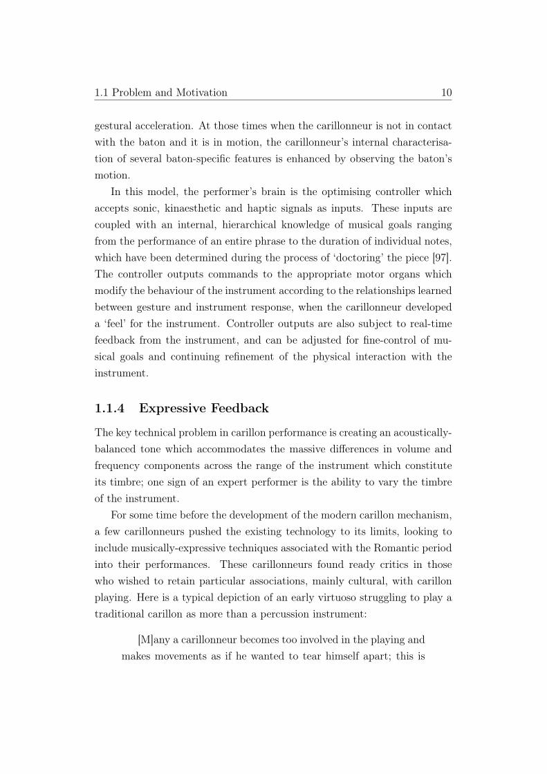
1.1.4 Expressive Feedback
The key technical problem in carillon performance is creating an acoustically-balanced tone which accommodates the massive differences in volume andfrequency components across the range of the instrument which constituteits timbre; one sign of an expert performer is the ability to vary the timbreof the instrument.
For some time before the development of the modern carillon mechanism,a few carillonneurs pushed the existing technology to its limits, looking toinclude musically-expressive techniques associated with the Romantic periodinto their performances. These carillonneurs found ready critics in thosewho wished to retain particular associations, mainly cultural, with carillonplaying. Here is a typical depiction of an early virtuoso struggling to play atraditional carillon as more than a percussion instrument:
[M]any a carillonneur becomes too involved in the playing andmakes movements as if he wanted to tear himself apart; this is

1.1 Problem and Motivation 11
the result of bad habits and a stupid desire for glory; it does nothave to go this far [78, p. 193].
The virtuoso carillonneurs looking to extend the instrument’s technicalrepertoire had been stymied by mechanical limitations. A significant lim-itation was the speed with which consecutive notes could be played; thiswas (and continues to be) a function of both the distance each baton musttravel and the force required to fully depress a baton. It was thought thatremoving this limitation would open the door to pianistic-style performances,and would also encourage other keyboard performers to consider learning thecarillon.
Figure 1.3: Flywheel carillon (images from [78]).
One attempted solution was the ‘Flywheel Carillon’, which used the prin-ciple of conservation of rotational momentum to offset the force required todisplace clappers. Shown in Figure 1.3, this instrument also replaced theclavier batons with a piano keyboard. Other adaptations included fitting hy-draulics to the keyboard mechanism in order to reduce the amount of forcerequired from the player. Such design innovations were never widely adopted.They tended to be mechanically unreliable but, more importantly, performersof the day had already begun to regard the carillon as an instrument capable

1.1 Problem and Motivation 12
of offering a wide dynamic range of expressive control; the tactile responseof the modern carillon clavier mechanism was crucial to such control.
The increasingly bravura performances of carillonneurs like Jef Denynchallenged carillon design, and by the early 20th century the modern crankmechanism was established as the standard alternative to the traditionalbreech mechanism. This new mechanism was despised by traditionalists,who claimed it was unnecessarily complex and encouraged an ‘unnatural’performance style [78].
As the crank mechanism was popularised by the advocacy and perfor-mances by Denyn at the St. Rombouts carillon in Mechelen in the early 20th
century [78, p. 242] it is notable that it was not a major technical innovationat the time. It first appeared in the 19th century, but languished for reasonsprincipally pertaining to maintenance: namely, because it had more mov-ing parts than the breech design it required more care, and its performancewould rapidly degrade when neglected. An advantage to these extra movingparts, though, was the opportunity to tune the performer’s mechanical ad-vantage over the instrument with judicious adjustment of linkage geometryand springs.
Denyn recognised that the heaviness of the instrument is an integral partof the carillon but also saw that, with attentive and precise maintenance,the relatively complex crank mechanism had the potential to balance theopportunity for virtuosic technique against the role of mechanically medi-ated feedback in a carillon performance. To this end he added return springsto increase the speed with which the baton would return to its home posi-tion, and forward springs which help the carillonneur pull heavier clapperstoward the bell. Both innovations enabled a faster playing style, referred toas the ‘Flemish style’ [78], without compromising a carillonneur’s capacityfor precise interaction with the mechanism.
This balance between springs, masses and linkage geometry which changefrom bell to bell is what characterises the feel and sound of the moderncarillon and why practice carillons are so inadequate for rehearsal.
1.1 Problem and Motivation 13
1.1.5 A Haptic Solution
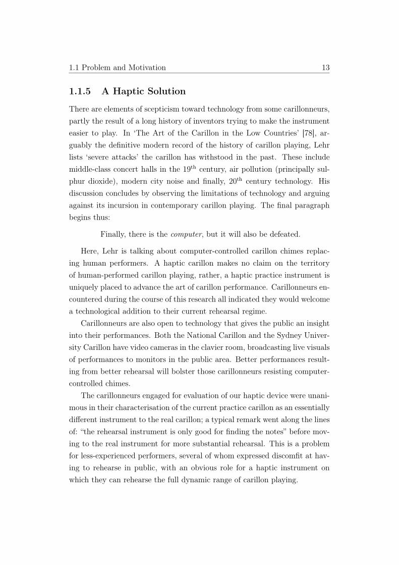
There are elements of scepticism toward technology from some carillonneurs,partly the result of a long history of inventors trying to make the instrumenteasier to play. In ‘The Art of the Carillon in the Low Countries’ [78], ar-guably the definitive modern record of the history of carillon playing, Lehrlists ‘severe attacks’ the carillon has withstood in the past. These includemiddle-class concert halls in the 19th century, air pollution (principally sul-phur dioxide), modern city noise and finally, 20th century technology. Hisdiscussion concludes by observing the limitations of technology and arguingagainst its incursion in contemporary carillon playing. The final paragraphbegins thus:
Finally, there is the computer, but it will also be defeated.
Here, Lehr is talking about computer-controlled carillon chimes replac-ing human performers. A haptic carillon makes no claim on the territoryof human-performed carillon playing, rather, a haptic practice instrument isuniquely placed to advance the art of carillon performance. Carillonneurs en-countered during the course of this research all indicated they would welcomea technological addition to their current rehearsal regime.
Carillonneurs are also open to technology that gives the public an insightinto their performances. Both the National Carillon and the Sydney Univer-sity Carillon have video cameras in the clavier room, broadcasting live visualsof performances to monitors in the public area. Better performances result-ing from better rehearsal will bolster those carillonneurs resisting computer-controlled chimes.
The carillonneurs engaged for evaluation of our haptic device were unani-mous in their characterisation of the current practice carillon as an essentiallydifferent instrument to the real carillon; a typical remark went along the linesof: “the rehearsal instrument is only good for finding the notes” before mov-ing to the real instrument for more substantial rehearsal. This is a problemfor less-experienced performers, several of whom expressed discomfit at hav-ing to rehearse in public, with an obvious role for a haptic instrument onwhich they can rehearse the full dynamic range of carillon playing.

1.2 Thesis Outline 14
In contrast, the most experienced performer in the surveyed cohort usedpractice instruments “virtually never, because they are very imperfect” andwas “always disappointed” when playing the real instrument afterwards. Af-ter evaluating the haptic device, the carillonneur proposed a secondary rolefor it, relevant to the experiences of a travelling concert carillonneur: a tem-plate for calibrating the feel of a real instrument. This was prompted bysurprise at how uneven the change in feel was across the range of the Na-tional Carillon, and they observed that a haptic carillon would provide aconfident perceptual baseline when making adjustments to a carillon’s feelduring maintenance or prior to a recital.
1.2 Thesis Outline
This thesis presents the design and implementation of a haptic baton thatcan simulate the force-feedback of any carillon baton. The haptic batonconstitutes a sensing/actuating system for force-feedback which is controlledby a virtual carillon model.
The major contribution of this thesis is this virtual model, which consistsof two separate models: a physical model of an individual carillon mecha-nism; and a model of variation in physical parameters across the range ofthe carillon. This combination of models allows the simulation of batonsabout which much is known as well as batons about which little is known.This is achieved by developing and validating precise models based on exten-sive data measurements, then generalising those models and validating thosegeneralisations with carillonneur evaluations.
Chapter 2 begins with a review of the literature regarding similar sys-tems, focusing mainly on those designed for musical expression. The reviewthen moves to methods of designing haptic systems which are actively sim-ulating real-world experiences and associated techniques for capturing andreplicating nonlinear dynamics of physical environments; Wavelet modellingis surveyed as a preview to its use later in the thesis for modelling batonswith significant discontinuities. A discussion of carillon performance tech-niques is followed by a review of the literature on mechanical impacts, which

1.2 Thesis Outline 15
provides the background for the development of a bell/clapper impact modelin a later chapter based on a correction to recent work by Fletcher et al. [42].
A precise model of an individual carillon mechanism is based on measure-ments taken of bell 4 at the National Carillon, and Chapter 3 presents ananalysis of the mechanical properties of this mechanism.
Chapter 4 develops a kinematically-based, nonlinear dynamic model forsimulating its motion and force-feedback. Alongside the development of thismodel, a linear model is developed based on a generalised form of the me-chanical analysis but does not require knowledge specific to the mechanism.
Chapter 5 describes the development of the haptic baton. A major com-ponent of this work is the method developed for sensing force applied bythe player, without the need for any additional force sensors. The positionof a wooden baton is controlled by a linear actuator, which is in turn con-trolled by the virtual baton model calculating baton motion in response tocarillonneur-applied force.
The mechanical structure identified in Chapter 3 provides a template forthe broader analysis of change in physical properties across the range of theNational Carillon presented in Chapter 6. Key physical properties of clappermechanisms are measured and then analysed according to historical modelsof bell design. These properties are shown to follow bell design principles andestablish a basis for parameter estimation for arbitrarily chosen clappers.
Chapter 6 also presents data describing a carillon’s haptic signature, whichencapsulates the force-feedback and motion characteristics that make up thefeel of a particular carillon. This haptic signature is used to validate theaccurate dynamic model for bell 4 in Chapter 7. The analysis of variation ofphysical parameters across the National Carillon is then used to populate thedynamic model for the simulation of other batons, which are also validatedagainst the respective haptic signatures.
Finally, the general model of the carillon mechanism, a generalised modelfor physical variation across the range of the instrument, and the perfor-mance of the haptic baton itself are quantitatively and qualitatively evalu-ated by carillonneurs at the National Carillon. These results are documentedin Chapter 7.

Chapter 2
Literature Review
The development of a haptic carillon draws on work from a number of re-search fields; novel musical instrument design, motor skill acquisition, hap-tic interaction, system identification, mechanical impact theory, and carillonperformance and design are all considered.
This thesis seeks to build a practice instrument that recreates the feel ofthe performance instrument for purposes of rehearsal. Haptic research showsthat force-feedback is an important factor in musical performance and othergestural tasks. Results from and research into haptic and novel instrumentdesign confirm this, and along with other haptic systems designed for percep-tual fidelity provide a guide to appropriate hardware and software tools forthe implementation of high-performance haptic devices. They also providea framework of evaluation criteria that places an emphasis on perceptualquality of the interaction between the user and the device.
At the hardware/control level, these instruments are informed by mecha-tronics, however, specialised stochastic control methods from robotics, likeKalman estimation, improve performance. At the software level, these instru-ments offer a panoply of methods for determining haptic responses, the mostrelevant being those that develop a physically-based computational modelof the target instrument. Of these, instruments with mechanical interac-tions between moving bodies form a template for dynamic modelling, andthe extent to which elements of such models can be simplified or generalised.

2.1 Musical Instruments and Haptics 17
However, some batons exhibit behaviour that is not easily incorporated intosuch models and the field of nonlinear haptic system identification is engagedto solve for these batons. In particular, a novel implementation of the Dis-crete Wavelet Transform (DWT) is used to model nonlinear components ofbaton behaviour. The development of modern carillon performance is thenreviewed alongside technological advances in the carillon mechanism itself,placing the technical requirements of the project in a musical context for theremainder of the thesis.
2.1 Musical Instruments and Haptics
Whether implicitly or explicitly, haptic musical instruments invoke the inter-active paradigms of acoustic machines that have been refined over centuries.At the core of any of these paradigms is the feedback loop between a per-former’s gesture and sensory feedback as a consequence of that gesture; thissensory feedback can be any combination of acoustic, visual and haptic feed-back.
Haptic feedback, from the greek word “haptesta” (to touch), is the com-bination of sensory cues along two channels. The tactile channel comprisessensations perceived through receptors in the skin and subcutaneous tis-sue. This includes pressure, vibration, temperature, softness, curvature andfriction-induced phenomena. The kinaesthetic channel is associated with anawareness of position, velocity and forces, or proprioception, and is sensedthrough receptors in muscles, tendons and joints [108]. The design of a sys-tem for haptic rendering is guided by these categorisations.
2.1.1 Vibrotactile Interactions
Depending on the nature of the instrument, haptic feedback can be felt inthe fingers, lips, feet and other parts of the body. Vibrotactile devices arethose which articulate tactile sensations directly onto, or in very close prox-imity to, skin; properly designed, these are characterised by an appreciationof the relevant psychophysics. Gunther and O’Modhrain developed a ‘com-
2.1 Musical Instruments and Haptics 18
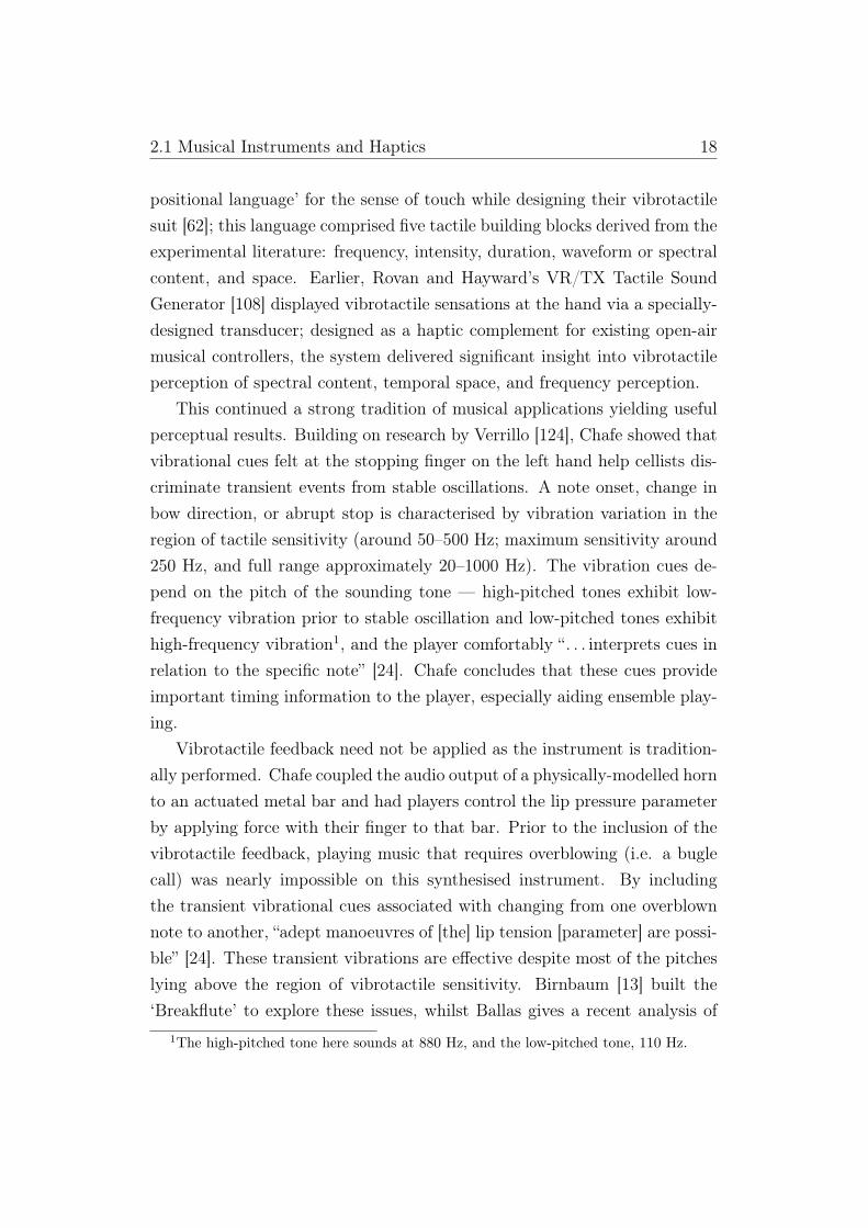
positional language’ for the sense of touch while designing their vibrotactilesuit [62]; this language comprised five tactile building blocks derived from theexperimental literature: frequency, intensity, duration, waveform or spectralcontent, and space. Earlier, Rovan and Hayward’s VR/TX Tactile SoundGenerator [108] displayed vibrotactile sensations at the hand via a specially-designed transducer; designed as a haptic complement for existing open-airmusical controllers, the system delivered significant insight into vibrotactileperception of spectral content, temporal space, and frequency perception.
This continued a strong tradition of musical applications yielding usefulperceptual results. Building on research by Verrillo [124], Chafe showed thatvibrational cues felt at the stopping finger on the left hand help cellists dis-criminate transient events from stable oscillations. A note onset, change inbow direction, or abrupt stop is characterised by vibration variation in theregion of tactile sensitivity (around 50–500 Hz; maximum sensitivity around250 Hz, and full range approximately 20–1000 Hz). The vibration cues de-pend on the pitch of the sounding tone — high-pitched tones exhibit low-frequency vibration prior to stable oscillation and low-pitched tones exhibithigh-frequency vibration1, and the player comfortably “. . . interprets cues inrelation to the specific note” [24]. Chafe concludes that these cues provideimportant timing information to the player, especially aiding ensemble play-ing.
Vibrotactile feedback need not be applied as the instrument is tradition-ally performed. Chafe coupled the audio output of a physically-modelled hornto an actuated metal bar and had players control the lip pressure parameterby applying force with their finger to that bar. Prior to the inclusion of thevibrotactile feedback, playing music that requires overblowing (i.e. a buglecall) was nearly impossible on this synthesised instrument. By includingthe transient vibrational cues associated with changing from one overblownnote to another, “adept manoeuvres of [the] lip tension [parameter] are possi-ble” [24]. These transient vibrations are effective despite most of the pitcheslying above the region of vibrotactile sensitivity. Birnbaum [13] built the‘Breakflute’ to explore these issues, whilst Ballas gives a recent analysis of
1The high-pitched tone here sounds at 880 Hz, and the low-pitched tone, 110 Hz.

2.1 Musical Instruments and Haptics 19
the neurological features of the limits of haptic perception [7].Nor need vibrotactile feedback be limited to the performer. Gunther and
O’Modhrain’s suit was worn by audience members in a series of concerts,Cutaneous Grooves (MIT Media Lab, 2001), and Gunther continues to de-velop cross-modal vibrotactile installations [61]. Merchel and Altinsoy [86]developed a whole body vibration system for evaluating the subjective ef-fect of vibration derived from the low-pass filtered audio during playback ofseveral different concert DVDs. Subjects judged reproduction with vibrationbetter than without, and favoured a low-pass filter cutoff of 100 Hz except inmusical examples where the spectral energy of bass-like sounds (bass drum,bass guitar) resided above 100 Hz.
2.1.2 Kinaesthetic and Proprioceptive Interactions
In the case of an instrument where the performer’s skin is not directly in con-tact with the vibrating medium, the haptic focus turns to the kinaestheticsensation and a performer’s proprioception. The object that the player in-teracts with is then a manipulandum that converts the player’s gesture toan acoustic consequence of some kinematic or force transformation. In thesecases, the audio output may not be an appropriate source for force/motiondata; for instruments like the piano, carillon or turntable, the behaviour ofthe manipulandum is almost entirely unrelated to the acoustic waveform.
Manipulandums, probes, and tactile simulation
The manipulandum’s role in a musical instrument has a nice analogue in tex-ture modelling and haptic rendering, an area which receives a lot of attentionfrom the haptic community. Displaying the frictional forces associated witha virtual object’s texture via a force-feedback device compensates in part forthe absence of tactile interaction. However, accurate tactile stimulation isrequired for high-performance haptic rendering and task-completion. Dost-mohamed and Hayward built a device to control pressure over a changingcontact area at the fingerpad in order to remove the “virtual probe” assumedin standard force-feedback devices [34]. Frisoli et al. developed a similar

2.1 Musical Instruments and Haptics 20
system, the HAPTEX, and demonstrated a “. . . significant deterioration inperception observed in virtual exploration of shapes through kinaesthetichaptic devices alone” [46]. Each of the following examples uses a haptic de-vice where a user holds a pen-like stylus to which a programmable force istransmitted.
Okamura et al. added observed vibrations to a simple wall model whichimproved the identification of simulated rubber, wood and aluminium [95]. Adental training system renders the textural forces arising from plaque usingmass-spring models, and students practice applying force with a vibratingplaque removal tool [116]. Adi and Sulaiman performed a 2D wavelet trans-form on visual images of different fabrics to create frictional-force modelswhich are more realistic than spectral models [3]. However, in ‘Feel the Fab-ric’, Huang et al. demonstrate that subjects easily recognise fabric texturesthat have been haptically modelled using spectral methods when combinedwith a separate but related acoustic model for simulating the sound of rub-bing different fabrics [71].
These texture-rendering systems have developed models of tactile sen-sation in order to simulate them through kinaesthetic devices; unlike, say,Chafe’s voice-coil actuated metal bar which featured a one-to-one mappingof audio oscillation to finger pad vibration.
A fascinating mix of cutaneous and kinaesthetic interaction is ‘ScannedSynthesis’, developed in 2000 by Verplank, Mathews and Shaw [123], whichis implemented on Verplank’s ‘The Plank’ [122], a 1-DOF, high-performancehaptic device. A wave shape is manipulated by the user at human hand fre-quencies whilst the wave shape itself is scanned at audio frequencies, allowingthe user to dynamically control timbre.
A similar dual-approach is taken with the haptic string devices, Nichols’VBow [92] and Florens virtual string instrument [44]. These works are no-table for recognising the complexity of performer/instrument interaction, andbuilding devices that do not over-simplify performer gestures simply to con-vert them into some usable control signal. Because of the high degree ofcontinuous expressiveness inherent in a stringed instrument, these haptic de-vices are designed to expose as much of the instrument physics as possible,
2.1 Musical Instruments and Haptics 21
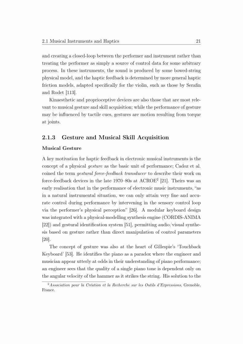
and creating a closed-loop between the performer and instrument rather thantreating the performer as simply a source of control data for some arbitraryprocess. In these instruments, the sound is produced by some bowed-stringphysical model, and the haptic feedback is determined by more general hapticfriction models, adapted specifically for the violin, such as those by Serafinand Rodet [113].
Kinaesthetic and proprioceptive devices are also those that are most rele-vant to musical gesture and skill acquisition; while the performance of gesturemay be influenced by tactile cues, gestures are motion resulting from torqueat joints.
2.1.3 Gesture and Musical Skill Acquisition
Musical Gesture
A key motivation for haptic feedback in electronic musical instruments is theconcept of a physical gesture as the basic unit of performance; Cadoz et al.coined the term gestural force-feedback transducer to describe their work onforce-feedback devices in the late 1970–80s at ACROE2 [21]. Theirs was anearly realisation that in the performance of electronic music instruments, “asin a natural instrumental situation, we can only attain very fine and accu-rate control during performance by intervening in the sensory control loopvia the performer’s physical perception” [26]. A modular keyboard designwas integrated with a physical-modelling synthesis engine (CORDIS-ANIMA[22]) and gestural identification system [51], permitting audio/visual synthe-sis based on gesture rather than direct manipulation of control parameters[20].
The concept of gesture was also at the heart of Gillespie’s ‘TouchbackKeyboard’ [53]. He identifies the piano as a paradox where the engineer andmusician appear utterly at odds in their understanding of piano performance;an engineer sees that the quality of a single piano tone is dependent only onthe angular velocity of the hammer as it strikes the string. His solution to the
2Association pour la Création et la Recherche sur les Outils d’Expressions, Grenoble,France.

2.1 Musical Instruments and Haptics 22
paradox is partly perceptual: fine control over note timing and impact veloc-ity creates the perception of phrasing, and from that, timbre. In particular,Gillespie argues that the haptic detent felt just prior to hammer let-off is avital cue in timing the conclusion and velocity of a key stroke. Consideredin these terms, familiarity with the instrument’s force-feedback is an obviousprecursor to articulate phrasing [53, p. 14].
Nichols’s VBow is another good example of the benefits to new-musicresearch when musical interaction devices are engineered as haptic feedbackdevices. Initially conceived as a gesture controller without haptic feedback[92], Nichols decided to include such feedback on learning of skill acquisi-tion results from O’Modhrain and Chafe and designed a system capable ofexploring far more.
Unlike a string or wind instrument, the piano and carillon have nocontinuous-time interactions; each instrument is dependant on the scalarproperties of impact time and impact velocity. These two instruments,though, are also distinguished by the complexity of the mechanism betweenthe the player and the eventual vibrating mechanism. The key or baton is amanipulandum for the hidden mechanism and lends itself quite naturally tosimulation through haptic technology.
Skill Acquisition
Learning a new or modified musical instrument involves the acquisition ofa hierarchy of motor skills represented at the lowest level by single gesturesto which an instrument’s dynamic response becomes intuitive. At higherlevels the organisation of these gestures into programmable and non-specificpatterns that can be called on and manipulated at will, and the highestlevel where these patterns can be organised into “temporal sequence uniquelydesigned to execute an individual piece of music” [97].
The wide range of dynamic and acoustical variance across the range ofthe carillon means carillonneurs find it more difficult than other musiciansto develop a reliable intuition for its dynamic response, which is itself proneto variation. The carillonneur partly combats this by having a good under-

2.1 Musical Instruments and Haptics 23
standing of the mechanics of their instrument; and, generally, the carillon hasundergone few adaptations that shield the carillonneur from its mechanicalworkings: working with the mechanism is a necessarily common part of earlycarillon pedagogy [57] [72] and composition [90].
Nonetheless, at the higher levels of proficiency the carillonneur ceases tobe actively (in real-time) concerned with feedback from individual gesturesat individual keys and instead relies on a learned intuition that anticipatesthe instrument’s state at a particular time.
This intuitive anticipation is key to expert performance because it allowsthe execution of sequences of gestures, or motor patterns, at a frequencythat exceeds the reaction time (RT) of the human motor system. This RT,generally determined to be between 120–180 msec, or less than 10 Hz [112],is the upper limit for human motor system to work in a closed loop control;that is, in order for a gesture scheduled for time tlater to adapt or respond tosome acoustical or mechanical feedback, that feedback must occur at a time(tlater − 120) msec or earlier.
A corollary to the intuitive anticipation described above is that an ex-pert performance becomes unstable when learned interaction constraints areviolated; this is the case whether a musician is performing on a traditionalinstrument, an electro-mechanical replica of a traditional instrument or anovel instrument, electronic or otherwise.
In their work on experimental force cues for musical performance, Berdahlet al. neatly sum up the challenge for the designer given these requirements:
If an assistive haptic interface ever takes an unexpected actiontoo quickly, then a musician who uses some elements of open-loopcontrol will not be able to respond appropriately, possibly makinga mistake. In practical contexts, we recommend simply that anassistive haptic interface be deterministic and relatively simple sothat no actions surprise the musician. [9]
In extensive experimental work, O’Modhrain [97] demonstrates that mu-sicians rely heavily on haptic interaction with a sound producing device, andhow novel instruments are often able to ‘train’ a performer to anticipate a

2.1 Musical Instruments and Haptics 24
particular type of haptic feedback produced within the constraints of hard-ware or software. This research leverages the fact that
[H]aptic feedback can support auditory feedback to informperformers of the consequences of their actions, playing a cru-cial role in the performer/instrument interaction loop. Where itexists, a mechanical coupling between player and instrument pro-vides a secondary sensory feedback channel through which muchinformation about an instrument’s state can be monitored. [97,p. 1]
In the case of entirely novel instruments a designer may eschew mechani-cal and acoustical interactions that require a burdensome level of hardware orsoftware components and design; that is not to say novel instruments do notfeature innovation, indeed they are often inspired by major artistic and/ortechnical insights of value to the many others in the instrument-buildingcommunity. Designers of electro-mechanical renditions of traditional instru-ments, though, must expend considerable effort replicating a mechanism thatin most cases has been refined over centuries to be the most efficient methodfor transferring a particular form of performer energy to acoustic energy.
This mechanism may be difficult to simulate, but dismissing the finerinteractions between the performer and instrument will “only continue thedisconnect felt by many performers with respect to available music inputdevices” (Scavone, discussing wind controllers that restrict breath pressurecontrol to slowly varying contexts [111]).
Perceptual research into human haptic interaction, specifically the per-ception of impedance, generally demonstrates the relative ease with whichhumans learn effective impedance exchange between limbs and real or virtualobjects [118].
Tsuji et al. analysed skill acquisition in the context of hitting a virtualtennis ball using a haptic system and EMG measurements on eight muscles inthe arm [120]. After about 100 trials, previously untrained subjects showedsignificant improvements in their ability to maximise the force with whichthey hit a moving ball — at the same time, they were able to coordinate

2.1 Musical Instruments and Haptics 25
muscle impedance more efficiently, minimising unnecessary muscle use. Thesubjects were also able to adapt their motion and impedance to changes inthe environment dynamics with little effort. In separate trials, the ball massand racket viscosity (drag) were changed and the subjects adapted in orderto maintain a maximum force on impact. In the high viscosity scenario, rapidacceleration of the hand is difficult so subjects would take a larger backswingto hit the ball with sufficient velocity; in the low viscosity scenario, subjectswould increase their own hand viscosity to maintain stability. In each caseof a changed ball mass, the subjects would adjust their hand impedance bystiffening their hand depending on the weight of the ball.
This last result is encouraging for a musical context like the haptic caril-lon, which will be expected to train performers for performance on arbitrarycarillons.
2.1.4 Haptically-Rendered Traditional Instruments
The Touchback Piano [53], the VBow [92], the Haptic Turntable [8], and theMIKEY (Multi-Instrument, Force-feedback Keyboard) project [93] are hap-tic instruments that are designed to replicate traditional instruments andtherefore to be immediately accessible to practitioners of the particular in-strument. These designs are intrinsically verified by virtue of being designedwithin the bounds of modern engineering practise and extrinsically verifiedwhen used by musical performers.
Performer Evaluations
However, there is not a great deal of literature relating to a performer’s per-ception when playing these instruments. The Touchback Piano, for instance,is verified primarily by comparing the motion of a grand piano mechanismwith a mass attached to the key with the offline simulated motion of themodel with the theoretical mass attached. Computational power at the time(1996) was insufficient to run the detailed equations in realtime, so a simpli-fied model (also used by Oboe in his 2006 MIKEY work [93]) was used forrealtime simulation. The simulated motions are a good match with those ob-

2.1 Musical Instruments and Haptics 26
served on the piano mechanism being modelled, but static mass force inputsare assessing only a narrow band of the instrument’s range.
More recent work by Gillespie et al. [54] models the driving pointimpedance of a human finger in the pressing of a piano key at the same timeas modelling the grand piano action using a set of linear transform func-tions. This approach seeks to incorporate finger behaviour ahead of time,pre-verifying the model, and is based on data collected from an experimentalrig that drives a mechanical piano action. The hybrid model is then sim-ulated offline and compared to measured data, finding excellent agreement.However, the system has not yet been tested in realtime.
Strong theoretical results are achieved in Hirschkorn’s 2004 work mod-elling the grand piano action [69], and his computational model is rigorouslytested using a range of force profiles used as input to this model; force profilesare captured when a pianist presses the key of a real grand piano playing soft,medium and loud notes. While demonstrating a high degree of accuracy inthe computational modelling, and the powers of contact analysis techniques,the model is never applied to a physical prototype and the opportunity totest the modelling against performer perception is unrealised.
A similar form of verification was used for the MIKEY project. In de-scribing the experimental regime, Oboe addresses why user-testing was notused in the final verification process:
The first type of experiment [for a haptic device] is usuallycarried out with a group of expert performers, but this has notbeen done in the MIKEY project, because the first tests withperformers were quite biased by the fact that no sound was gen-erated when acting on the key, so the correlation between hapticperception and generated sound was lost. [93, p. 47]
The VBow does include a very strong component of sound reproductionand audio synthesis, however, its function as a substitute for the traditionalviolin is not explicitly determined through user-testing. Nichols advocatesmore of an experimental role for the instrument in performance; the instru-ment is designed to give the composer an opportunity to use kinaesthetic

2.1 Musical Instruments and Haptics 27
feedback along with audio as a compositional element. In this way, Nicholsenriches his device by directing it toward taking advantage of the type ofresearch undertaken by O’Modhrain and Chafe [99].
The Haptic Turntable actively sought to cross the boundary betweenreplicating the sensation of the real instrument, and adding non-trivial hapticcues based on the audio content, matching beats for instance. The literaturedoes not give a detailed account of performer evaluations, although the lone-turntable component was apparently well-received, but the haptic cues notas much.
There is a developing body of understanding regards the evaluation ofdigital instruments, particularly from the NIME (New Interfaces for MusicalExpression) community. In a recent article, O’Modhrain explicitly tackles theevaluation of digital musical instruments within a broad framework includingperformers, audiences, designers and manufacturers [98]. The framework ismainly intended for novel instruments, but the evaluation goals she identi-fied of enjoyment, playability, robustness and achievement of design speci-fications, apply to haptically-rendered traditional instruments, especially ifthey are competing with other non-haptically enabled practice instruments.In particular, the goals of maximising enjoyment and playability are goodcandidates for distinguishing haptic practice instruments.
From the performer’s perspective, enjoyment is evaluated through reflec-tive practice, development of repertoire, long-term engagement, whilst thedesigner can tune their instrument to maximise enjoyment by observing per-formers’ interactions, with questionnaires and other informal feedback. How-ever, the increased complexity in a haptic instrument raises issues regardingrobustness, and meeting playability expectations that arise from imitatinga real instrument. These goals requires quantitative evaluation of the userinterface, mapping and hardware/software testing.
2.1.5 Stable Haptic Interactions
An instructive feature of research into haptic perception generally is theextraordinary level of empirical testing required to develop a model that suits

2.1 Musical Instruments and Haptics 28
a user’s expectation. Brown and Colgate [18] [19] published several worksin the 1990s that developed the baseline for limits of effective impedancedisplay. Initially considering the implementation of virtual walls in 1994,the perceptual qualities of which had been investigated slightly earlier byRosenberg and Adelstein [106] and Fasse [39] among others, Colgate [28]developed the concept of ‘Z-width’ as a generalised measure of the dynamicrange of discretely-controlled impedance display of a particular haptic deviceand acceptable limits for human interaction.
The development of stability criteria and the concept of virtual couplingfor haptic display systems [28] [19] [88] [1] has greatly increased the rangeof haptic applications, particularly in cases where the nature of a virtualenvironment is not known a priori, or it changes over time. A well-designedvirtual coupling will guarantee that interaction between an operator and apassive virtual environment — like those based on physical systems, notwithstanding some issues that may arise from numerical integration [18] [2]— will be stable, no matter how complex the virtual environment.
Colgate and Brown’s Z-width focused on designing virtual environmentsthat themselves would guarantee stability during interaction [28]. This con-tained a valuable insight, however, that accurate modelling of the virtualenvironment alone is not sufficient to guarantee a realistic haptic display:
It is generally argued that the dynamics of a haptic inter-face should be dominated by the virtual environment (which is,after all, the programmed behaviour we wish to display). Un-fortunately, th[is] notion places focus on mimicking the govern-ing equations of physical systems, but not on obeying underlyingphysical laws (such as conservation of energy). Adding physicaldamping helps the sampled-data system to behave as physicallaw would dictate. [28, p. 3207]
Colgate and Brown’s remarks confirm the general schema to modellinghaptic systems described by Maclean in [84], that a theorised mathemat-ical model of the system alone is not sufficient to guarantee a stable orperceptually-realistic haptic display. It also supports the evaluation frame-

2.1 Musical Instruments and Haptics 29
work proposed by O’Modhrain [98]: devices need to be evaluated againsta range of criteria, and from several perspectives. Indeed, in a statementthat could easily be applied to the digital musical instruments to whichO’Modhrain refers, particularly where the designer is the primary performer,Maclean says: “perceptual matching which relies on the designer’s own hap-tic perception is the ‘holy grail’ of emulation fidelity. [However, t]he relianceon haptic perception is good for fidelity but poor from the concern of aquantitive mapping between real and virtual environments” [84].
Adams and Hannaford have since extended and generalised the conceptof virtual coupling from mainly being applied to impedance displays (mea-sured motion, output force), to admittance displays (measured force, outputmotion), and analytically separated the impedance of the virtual environ-ment being modelled, and that of the virtual coupling [2] [1]. Their two-portimmittance analyses based on Llewellyn’s stability criteria [81] result in con-ditional expressions that permit fine-control over these relationships. Theyanalytically demonstrate that the designer must make a trade-off in perfor-mance when simulating free motion, and performance when simulating rigidbody motion.
In admittance displays, this trade-off involves the position-control loopgain, the impedance of the physical actuator/manipulandum, and theimpedance of the virtual environment. It remains the case, though, thata performance trade-off is always required to guarantee stability, althoughthese can be tailored to the virtual environment without adjusting that en-vironment itself [1]. More recent applications of admittance display demon-strate that a virtual environment can display significant complexity, with acombination of free motion and rigid constraints, as in the Cobot Hand Con-troller by Faulring et al. [40]. Other researchers [83] [79] have demonstratedthat a manual tuning of a virtual coupling network is sufficient to guaranteestability in systems where the virtual dynamics are known.

2.1 Musical Instruments and Haptics 30
2.1.6 Manual Tuning of Force Sensing With Kalman
Filtering
In an admittance display scheme, instability arises when the system respondsto large changes in force input with large commanded accelerations [66]. Thisproblem is particularly associated with small virtual masses where there islittle virtual inertia to prevent large accelerations [83] [19]. A virtual couplingscheme could be developed and tuned to accommodate that entire range,however tuning part of the emulation fidelity related to the sensitivity of anadmittance display need not be left solely to the designer. A novel forcesensing method based on multi-signal fusion and Kalman filtering allows theuser to adjust the sensitivity of the interaction themselves. It also removesthe need for a force sensor apart from the actuator itself.
Force-sensing from disturbances to position-controlled robotic systemshas become increasingly popular in robotics [114] [103], eliminating the needfor wrist force sensors or other sensors at the end-effector, which themselvesare prone to noise contamination [80]. In these systems, the current com-manded to the actuator from the servo is monitored for disturbances due tothe external application of force. When an external force is applied to a stiffposition-controlled manipulandum that is driven by a D.C. motor, the cur-rent in the actuator increases proportionally with that force [89]. However,this current signal is contaminated with process and measurement noise, andalso includes forces due to the motor components themselves (inertia, frictionand gravity acting on the stroke mass), and requires some processing beforeit can be employed for control.
In research focusing on a black-box robotic system, Naghdy et al. devel-oped Auto-Regressive-Integrated-Moving-Average (ARIMA) models for sim-ilar control noise which could forecast future force signals [89]. The errorbetween the forecast value and the measured value is fed into a CumulativeSum Control Chart (CUSUM) which can detect significant variation; such asignificant variation indicates the presence of force not accounted for by thenoise model. Used in a compliant control scheme, this technique improvedthe performance of industrial robots during object insertion tasks [89]. This

2.2 System Identification for Haptic Display 31
technique required some pre-filtering of the force signal in order to conditionthe signal for time-series analysis; in Luk [82], a low-pass filter with a cut-offof 20Hz was used. This, however, is well below the perceptual threshold fortransparent haptic interaction.
More recent research has shown the Kalman state estimator to be a veryeffective method of removing process and measurement noise from one ormany digital signals. The implementation of a Kalman estimator requiresa discrete model of the process or system, whose state is being estimated,which would seem to put it at a disadvantage to more general black-box mod-els. However, the literature in this area shows that the Kalman filter is quiterobust to the selection of process models: Yun et al. [131] filtered accelerom-eter data used in motion tracking using a first-order linear process model forhuman limb movement, a significant simplification that nonetheless yieldedgood experimental results. On the other hand, Hernández [67] developeda mass-spring-damper model of the internal mechanics of an accelerometerand used that as the process model for Kalman filtering, also yielding a gooddegree of noise reduction.
The extent of noise reduction in the Kalman filter is determined by inputvalues for process and measurement noise covariance [58]. Because externaldisturbance from user-applied force is also considered noise, these parametersalso determine the responsiveness of the haptic interaction. Unlike a low-pass filter, there is a reasonably small time lag associated with increasing thesmoothness of the signal [58] [131].
The Kalman filtering method allows the user to perform perceptual fine-tuning of the responsiveness of the interaction, accounting for variation inthe virtual mass in individual batons; this also allows the designer to focuson quantitative evaluations of the virtual simulation of the real environment.
2.2 System Identification for Haptic Display
One method for establishing a baseline from which to make quantitative eval-uations, at least with regards to the dynamic behaviour of the instrumentbeing modelled, is to construct a model of the physical system itself. How-

2.2 System Identification for Haptic Display 32
ever, this model will necessarily be a simplification of the relevant systemelements, and will require tuning to best approximate the behaviour of thesystem.
A Priori Modelling
The implicit theme in Gillespie’s earlier work on the Touchback Piano [53],and explicit in Hirschkorn’s theoretical model of the grand piano [69], is thatgiven an accurate description of a particular grand piano mechanism it ispossible to construct a set of equations that will model the behaviour ofthat mechanism. Oboe [93] used a simplified model Gillespie developed forrealtime testing and, presumably after parameter tuning, achieved agreementbetween simulation results and experimental data.
Hirschkorn’s work, though, demonstrates that it is extremely difficult tobuild a physical model of the piano’s complex mechanism from a theoreticalbasis alone. His thesis presents a rigid multi-body model of the grand pianoaction, precisely derived from the physical properties of an actual mechanism.He was also able to quite accurately fit contact force models describing theinteractions between these bodies; his access to the mechanism allowed in-dependent fitting of a hysteric, velocity-dependant contact force model foreach interaction. The full model’s motion was compared against the motionof the real mechanism in response to four dynamic force inputs from a pianistranging from piano to forte. The model performed very well for large blows,but less so for gentle or quick double-blows. His sensitivity analysis showedthat the model had an increased sensitivity to friction at low speeds, but hewas unable to retune his model to account for this whilst retaining agreementwith quicker hits.
Hirschkorn’s co-authors, McPhee and Birkett [70] were involved in thelater work of Vyasarayani et al. [126] and Izadbakhsh [74] which improvedon these results by modelling the hammer shank as a flexible body; in partic-ular, a more sophisticated model of the hammer-string impact also improvedmodelling of the hammer motion after impact [125]. However, the earlierwork of Hayashi et al. [65] showed that a piecewise linear mass-spring model
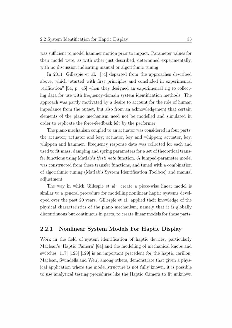
2.2 System Identification for Haptic Display 33
was sufficient to model hammer motion prior to impact. Parameter values fortheir model were, as with other just described, determined experimentally,with no discussion indicating manual or algorithmic tuning.
In 2011, Gillespie et al. [54] departed from the approaches describedabove, which “started with first principles and concluded in experimentalverification” [54, p. 45] when they designed an experimental rig to collect-ing data for use with frequency-domain system identification methods. Theapproach was partly motivated by a desire to account for the role of humanimpedance from the outset, but also from an acknowledgement that certainelements of the piano mechanism need not be modelled and simulated inorder to replicate the force-feedback felt by the performer.
The piano mechanism coupled to an actuator was considered in four parts:the actuator; actuator and key; actuator, key and whippen; actuator, key,whippen and hammer. Frequency response data was collected for each andused to fit mass, damping and spring parameters for a set of theoretical trans-fer functions using Matlab’s tfestimate function. A lumped-parameter modelwas constructed from these transfer functions, and tuned with a combinationof algorithmic tuning (Matlab’s System Identification Toolbox) and manualadjustment.
The way in which Gillespie et al. create a piece-wise linear model issimilar to a general procedure for modelling nonlinear haptic systems devel-oped over the past 20 years. Gillespie et al. applied their knowledge of thephysical characteristics of the piano mechanism, namely that it is globallydiscontinuous but continuous in parts, to create linear models for those parts.
2.2.1 Nonlinear System Models For Haptic Display
Work in the field of system identification of haptic devices, particularlyMaclean’s ‘Haptic Camera’ [84] and the modelling of mechanical knobs andswitches [117] [128] [129] is an important precedent for the haptic carillon.Maclean, Swindells and Weir, among others, demonstrate that given a phys-ical application where the model structure is not fully known, it is possibleto use analytical testing procedures like the Haptic Camera to fit unknown
2.2 System Identification for Haptic Display 34
variables to the model, even when some parts are nonlinear.The Haptic Camera is a position-controlled force probe which records
force and displacement data, and is capable of force display. Maclean’s as-sociated haptic characterisation procedure assumes that the system beingmodelled is nonlinear and globally discontinuous, but is linear in regionsdemarcated by position trajectories; these linear regions are modelled asmass-spring-damper systems. The start and end of these linear regions aredetermined by finding peaks in the second-derivative of measured force, sig-nifying a nonlinear change in force. A model of the entire system is thengiven by:
F = M(x)a+ B(x)v + K(x)x+ x0(x) (2.1)
where M,B,K and x0 are vectors containing region-specific values for mass,damping, springiness and force offset.
Maclean developed a data collection procedure that allowed her to fitparameters one after the other, by considering the model in parts. The hap-tic camera was programmed with three ‘position-trajectories’: quasi-static,constant velocity, and constant acceleration. The quasi-static trajectory hadalmost zero velocity and acceleration, removing mass and damping as sourcesof force, allowing the calculation of values for position-dependant vectors Kand x0 alone. The constant velocity trajectory is then used to determinethe velocity-dependant vector B with the previously determined position-dependant vectors; finally, vector M is calculated based on the constantacceleration trajectory and previously calculated vectors. Gillepie’s recentpiano modelling echoes this process of defining a complex model by collectingexperimental and fitting data at different operating points in the mechanism.
Colton and Hollerbach [29] [30] generalise this piecewise 2nd order con-tinuous approach by demonstrating that any model F = f(x, v, a) whereforce-feedback is a nonlinear function of motion variables can be consideredlocally linear, and approximated as a linear mass-spring-damper model atevery position x, with separate values again for negative and positive veloc-

2.2 System Identification for Haptic Display 35
ity:
F =
m+(x)a+ b+(x)v + k+(x)x+ F+0 (x), v > 0
m−(x)a+ b−(x)v + k−(x)x+ F−0 (x), v < 0(2.2)
This model is then fitted to measured data using an exponentially-weightedleast-squares recursive algorithm.
Maclean’s later work with Swindells [117] includes the Karnopp frictionmodel, and adds a sinusoidal nonlinearity, to describe the feel of a rotationalknob with constant mass M :
τ = Mθ + τfric( ˙θ+, ˙θ−) + Apos sin(θ/Ppos + Spos) (2.3)
The final term models detents using a sinusoid containing parameters foramplitude, period, and phase shift, and the authors note that non-sinusoidaldetents could be modelled using other position-based functions. Prior tothis, the technique of modelling haptic detents with sinusoidal functions hadfound a musical application in Beamish’s Haptic Turntable [8] (with Macleanand Fels).
The function τfric encapsulates the Karnopp friction model. It is a functionof velocity and the sum of non-frictional torque applied to the system, andincludes Coloumb (dynamic), static and viscous friction while allowing forasymmetric friction values for positive and negative forces. The Karnoppmodel has proven to be effective for both the identification and haptic displayof friction [105].
Several authors in this area note that the act of selecting an appropriatemodel is a sensitive one. Swindells et al. observe “[t]he most detailed modelwill not produce the best results because additional parameters will . . . strainthe fitting algorithm’s ability to fit values to a certain level of consistencyand quality” [117]. Further, it is not always necessary to use a model that isentirely linear.
The parameter estimation used for the rotational knob model is a goodexample of mixing techniques; the parameters M , Apos and the Karnoppfriction coefficients are fitted using Matlab’s mldivide (“\”) function, whichis an unconstrained linear least-squares solver, and numerical function min-
2.2 System Identification for Haptic Display 36
imisation was used to fit Ppos and Spos, with Matlab’s lsqcurvefit. Richard’swork [105] shows that with appropriate preparation, the Karnopp model co-efficients can be reliably estimated by finding a linear least-squares solution.
Weir et al. designed a measurement apparatus that captured force, posi-tion, velocity, acceleration and sound data from various switches [128]. Themeasurements were used to create a set of graphical representations of whathe termed the ‘haptic profile’ of these switches, in which these data are con-sidered as functions of each other rather than time. This encourages anintuitive appreciation of haptic features relevant to the feel of switches, like‘clicky’, ‘smooth’, and ‘mushy’ [128, p. 1] that would otherwise be more dif-ficult to determine from time-domain representations of the data sets alone.
Weir does not use the data to fit any particular model, but rather presentsthe analytical method as a tool for designers to fine-tune their own models forthe force characteristics of mechatronic systems [129]. From the point of viewof nonlinear parameter estimation, these projections provide a sanity-checkwhen working with structured models that are based on kinematic analysis.
In Chapter 6 of this thesis, Weir’s haptic profile is developed into a ‘hapticsignature’ by including time-domain data that shows a baton’s tendency tobounce repeatedly after impact, and additional force data relating to thechange in nature and magnitude of force-feedback across the range of thecarillon.
Wavelet Modelling
Often, the dynamics of a system may be largely unknown prior to data col-lection as in the case of the examples and scenarios reviewed above. However,much can be predicted about the dynamics of a carillon mechanism withoutobserving it directly. One feature of the carillon mechanism is that it is de-signed to give a smooth force response throughout a stroke, so the dynamicsof an ideal stroke can be closely simulated by approximate models which donot change in structure. It is not uncommon, though, for a baton to exhibitbehaviour that cannot be accounted for by the structural model; in thesecases a nonlinear modelling method like wavelet networks can be added to

2.2 System Identification for Haptic Display 37
the structural model in order to account for these deviations.In 1998, Miller and Colgate [87] developed wavelet networks for character-
ising haptic systems that were mainly linear, but exhibited discontinuities, ordetents, in their force/displacement profile. This approach has the advantagethat wavelet analysis is specifically designed to capture discontinuities. Fur-ther, a wavelet network is simply the linear combination of weighted waveletfunctions, meaning that wavelet coefficients can be calculated by finding alinear least-squares solution to the measured data. In their example, a non-linear function relating force to displacement was modelled by combining theweighted wavelet functions with a constant and first order linear term.
Prior to this, Pai and Reissell developed an algorithm based on waveletanalysis to determine the boundary curves of visual images for haptic inter-action [100]. The curves were modelled as solid objects, which produced forcewhen pushed with a haptic interface, allowing a user to explore the shapes.More recently, Adi and Sulaiman [4] used wavelet networks to analyse 2-dimensional visual information which can then be used to generate haptictextures.
Wavelets, and the Discrete Wavelet Transform (DWT) in particular, areoften used for noise filtering. The multiresolution decomposition at the heartof the DWT is ideal for separating noise from signal. In 1994, Berger andNichols [11] used wavelet analysis to restore an 1889 wax cylinder record-ing of Brahms playing his own work. They note: “the poor quality of thecylinder recording resulted in a general consensus that the recording wasnot of significant musicological value. By applying orthogonal trigonometricand wavelet-based analysis techniques we were able to reconstruct enoughmeaningful musical data for us to challenge this long-held view”. Waveletscontinue to be applied to audio signals; Guangbo et al. combined waveletanalysis with pattern recognition for feature-based signal de-noising [59], andBrömer implemented realtime wavelet analysis for multiresolution analysis ofmusical audio signals [15].
Multiresolution analysis is particularly powerful for removing noise froma signal which itself has significant discontinuities. Generally, the removalof noise with wavelet analysis is referred to as smoothing, which consists of

2.3 Playing the Carillon 38
decomposing the noisy data into a wavelet basis, suppressing wavelet coeffi-cients below a certain amplitude, and then transforming the data back into itsoriginal domain. Smoothing techniques can be as simple as hard threshold-ing, which simply removes coefficients with values smaller than some thresh-old, or more sophisticated, like the non-negative Garrote smoothing [49].
Durand and Froment [37] [36] developed a smoothing technique whichminimises the total variation (TV) in a signal, based on the algorithm de-veloped by Rudin et al. for de-noising images [109]. This approach avoidsoscillations in the vicinity of a signal’s discontinuities which arise with otherforms of thresholding. This is referred to as the pseudo-Gibbs phenomena af-ter the Gibbs phenomena associated with Fourier-based thresholding, whichsimple forms of wavelet thresholding nonetheless outperform [27]. Whilstthe pseudo-Gibbs phenomena does not in itself increase the error betweenan original noiseless signal and the de-noised signal, Durand and Fromentnote that the oscillations affect the visual quality of the result; in a hapticcontext, where the signal related displacement to force, such oscillations areundesirable.
However, the prospect of realtime smoothing of a discontinuousforce/displacement function depending on some other user-specified oralgorithmically-determined parameter, has many potential applications inmodelling nonlinear haptic systems. In Chapter 6, a thresholding techniqueis developed based on the baton’s velocity, after haptic signature analysisof baton 7 showed a strong correlation between the velocity of a stroke andthe sensation of ‘roughness’ in the stroke not accounted for by the Karnoppfriction model.
2.3 Playing the Carillon
2.3.1 Modern Carillon Mechanism and Performance
Modern carillon performance has its origins in the late 19th century, whena deeper understanding of bell tone and increasing ability of bell-foundersto control tunings [6] [68] was emerging alongside the romantic musical pe-

2.3 Playing the Carillon 39
riod. More accurately and consistently tuned bells increased the potentialfor sophisticated timbral control as part of musical expression, and perfor-mance techniques developed for other instruments during the romantic periodshowed how this potential could be realised.
Virtuoso carillon performance as we know it depended on a technologicalinnovation in carillon design: the transition from the breech mechanisms tothe bell-crank mechanism. Jef Denyn, a carillonneur born in Mechelen inthe late 19th century, is generally credited with popularising the bell-crankmechanism who took up and popularised the use of the bell-crank mechanismfor manual carillon performance [78]. Until Denyn, the bell-crank mechanismwas only used to strike the automated hammers for low bells.
The Breech Mechanism
Prior to the bell-crank mechanism, the standard carillon was made up of aseries of breech mechanisms, one of which is shown in Figure 2.1. The breechmechanism provided the carillon designer with little control over the forcerequired to play different clappers. The design required return springs, whichworked against the carillonneur, and had no place for forward springs whichmight assist the carillonneur on heavier bells.
Performing with the breech mechanism required great physical exertion,even when not aiming for virtuosity. This limitation meant that the instru-ment was perceived as a member of the percussion family; the Dutch in par-ticular developed a contrapuntal style of performance — which avoided sig-nificant dissonances from big chords — for the performance of harmonically-stable religious and folk songs [91]. And, because of the physical require-ments, only the most fit carillonneurs could even attempt virtuosic perfor-mances on breech carillons. The English musicologist Hugh Reginald Haweisheard Denyn’s father, Adolf, perform in Mechelen, and observed that hisplaying was particularly dexterous and that he was in excellent physical con-dition and regularly exercised with heavy clubs. He wrote that Adolf wasable to create great contrast between piano and forte, and he had a novelmethod of playing the melody in the bass bells to the accompaniment of

2.3 Playing the Carillon 40
Figure 2.1: Breech system in its most elaborate form. The player pulls the batonwhich pulls the clapper against the bell wall. A spring behind the clapper helpspull it away from the bell after impact. This system did not allow for a forwardspring to assist the carillonneur. (Figure from Lehr [78])
short demi-semiquavers in the high bells [78, p. 222]. This is the precursorto the Flemish virtuosic style of playing that arose in the early 20th century.
The general tendency to view the carillon as a percussion instrument sawthe desire for virtuosic performances greeted with suspicion, along with anearly 20th century push to convert carillons from breech to bell-crank mech-anisms. The following quote is from an early 20th century Dutch committeeformed to consider adopting the new technology:
[S]ince a tone cannot be held at will for any given time ona bell, something which seemed to be the main aim of the pro-posed changes, by means of the so-called Flemish tremolo. Atremolando on bells violates the original carillon character andalthough a tremolo can occasionally give a pleasant effect, itsmultiple use would soon become very boring. [The committee

2.3 Playing the Carillon 41
believed the] Flemish style was obviously inferior to the presentDutch style and the danger was real that it would degenerate intodubious virtuosity. [78, p. 243]
Bell-crank Mechanism
Although Jef Denyn popularised the bell-crank mechanism, he was not itsinventor. The primary drawback of the crank mechanism for manual perfor-mance prior to his intervention was the leisurely pace with which the clapperwould return from the bell after an impact; this affected how quickly a car-illonneur could repeat a note, and diminished the repeatability of impactvelocities by limiting the range of baton motion the carillonneur had op-portunity to finesse its speed. Denyn overcame this limitation by includingsprings, and taking particular care to keep the increased number of mechan-ical components well-maintained.
This innovation opened the door for sustained periods of tremolo, andthe associated increase in timbral and harmonic possibility, though virtuosicmusical expression through timbre was not conditional on well-tuned bells.Lehr reports: “It is said of Jef Denyn that when playing certain love songsand when the pain caused by the unattainable lover had reached a peak, hewould use a very out-of-tune bell in his carillon to accentuate this even more”[78].
However, developments in bell tuning technology during the 20th centuryhave increased the control bell-founders have over bell pitch and tunings.In particular the computational finite-element modelling of church bells byPerrin and Charnley in 1983 [101] allowed a precise understanding of themodal interactions within a bell. This has been incorporated into refinementof existing bell designs, and the creation of novel designs where the pitchsensation is pre-determined [85]. A thorough analysis of pitch sensations andbell-founding theory is given in Hibbert [68], along with tuning data for over2,000 bells. Bagot provides a historical context for the development of thebell [6].
These innovations in bell-tuning have focussed the minds of composers

2.3 Playing the Carillon 42
Figure 2.2: Early form of the bell-crank system. The clappers are secured againstsideways motion with cables and return springs pull the clapper quickly away fromthe bell. Mechanical advantage between the player and the clapper can be adjustedby altering the lengths of the crank rods; the rod going to the clapper is typicallyconstrained to be an L-shape in order to achieve the greatest possible horizontaldisplacement. (Figure from Lehr [78])
and performers/improvisers. Narushima [90] provides a good discussion onthe musical aspects of the tuning systems in carillons, and Gordon [56] in-corporates these musical aspects into performance styles.
Easing the physical requirements for playing low bells in particular greatlyincreased their dynamic range, and a well-balanced mechanism exposes thefull dynamic range of the entire instrument. Modern performance techniqueis tuned to take advantage of the instrument’s dynamic range.
In a nice analog to haptic perceptual research, the typical testing scenariofor virtual wall implementations — i.e. subjects ‘explore’ the wall with thegoal of determining, and assessing various physical properties like stiffness,

2.3 Playing the Carillon 43
hardness, crispness etc. — is very similar to the familiarisation a carillonneurundertakes with an unfamiliar carillon. Hurd describes a process of applyinga gentle force, mainly from the weight of one’s limbs, that brings the batonto rest at approximately 1/3rd of its total displacement, then releasing thisforce and allowing the baton to return to its rest position; this is repeated anumber of times until he develops a muscle-memory for the baton. The bell istypically not sounded until near the end of this process; the heaviness of thebaton at that partial displacement provides the carillonneur with sufficientinformation for the rest of the stroke.
Even in normal playing there is a small amount of ‘exploration’ beforeevery stroke; from “Playing the Carillon: An Introductory Method” by JohnGouwens:
As much as possible, the hands should be prepared and atrest atop the keys before commencing the stroke. For playing atmezzo piano or louder, one should begin the stroke with just aslight forward motion, mostly meeting the weight of the actionand clapper with the weight of one’s arms. Since the player nor-mally sits at an incline, the weight of the arms will naturally tendto move forward. The key and the hand must start in motion to-gether. Players who come crashing down on the keys subject theinstrument and their hands to considerable punishment, and theresulting sound is often harsh and ugly. [57]
Gouwens’ comments are supported by modern research into the mechan-ical interaction between the clapper and bell during impact.
2.3.2 Clapper and Bell Impact
The vibrations and resonances of bells have been exhaustively studied butonly recently has this understanding been applied to the dynamics of theclapper motion during and after impact with the bell. Whilst the sonicbehaviour of the carillon bell upon impact is not of immediate interest to ahaptic simulation, research into the vibrational modes of wave propagationin the bell does relate to clapper motion after impact.

2.3 Playing the Carillon 44
Fletcher and Rossing, in The Physics of Musical Instruments [43], de-scribe the vibrational modes of carillon bells and provide methods foranalysing and predicting a bell’s harmonic partials based on the geometryand physics of the bell. In later work at the National Carillon, Canberra,Fletcher et al. conduct an analysis of the impact dynamics between the clap-per and the bell [42]. The paper verifies that the sound spectrum of thebell, particularly the frequency of maximum excitation, changes significantlydepending on the state of re-voicing.
Over the course of repeated impacts, the clapper develops a flat surfacecalled an impact damage flat at the site of impact with the bell. Clappersare periodically re-voiced to remove this damage flat, because it affects thetone. Fletcher et al. demonstrated that the sound spectrum of a re-voicedclapper contained fewer and stronger peaks, and the strongest part of thespectrum, the frequency of maximum excitation, was lower in frequency fora re-voiced clapper. Fletcher’s analysis of bell 29 shows an adjustment of thisfrequency from 4kHz for an unvoiced clapper to 2kHz for a re-voiced clapper.This frequency is correlated with how ‘bright’ the instrument sounds.
Deriving their own set of equations from materials and impact theory,mainly from Goldsmith [55] and Skudrzyk [115], Fletcher et al. also demon-strate that the brightness of the bell and the length of the time the clapper isheld against the bell are both strongly correlated with the extent of damageflat of the clapper [42]. The contact time determines the velocity of the pulsearound the bell, which then determines the harmonic nodes that are excitedby the impact [107]. They show that for a clapper of damage flat greater that5mm, the contact time ceased to be dependant on the velocity of an impact,meaning that a carillonneur playing with a damaged clapper has almost nochance of effectively controlling the tone of the instrument.
Their paper makes a second claim: that the clapper is in fact at restagainst the bell surface until a return vibrational pulse pushes it away, andthe velocity of this pulse is affected by the frequency of maximum excitation,f , which they calculate by performing a Fourier transform of their calculatedforce curve. However the validity of their results is undermined by an errorin calibrating their model to the more accurate Hertz impact law. This

2.3 Playing the Carillon 45
significantly alters the magnitude of forces predicted by their model, buthas a smaller influence on their predictions of contact time based on wavevelocity.
2.3.3 Impact Force Analysis
A force analysis of the collision between a clapper and bell invokes a verycommon scenario in the literature: a sphere impacting on a flat surface mas-sively greater in mass than that sphere. Hertzian impact theory, as presentedin Goldsmith, is a quasistatic procedure for determining an idealised elasticimpact force between such bodies from which contact time τ , maximum forceFmax, maximum compression αm and contact area a can be predicted [55].It models the interaction force as a nonlinear spring:
F = kα3/2 (2.4)
where parameter k is fully determined by the geometry and physical prop-erties of the colliding bodies, and α = h1 + h2, called the approach, is therelative compression of the two bodies, where hi denote the respective com-pressions of the two bodies.3
It is common practice when developing or adapting a model for describingcollisions to compare its performance in scenarios that partly or fully overlapwith the classic Hertzian scenario. This serves two main purposes: to contin-ually update the known limitations of the widely-used Hertzian theory; and,to validate new models by showing them to produce results in agreementwith the simple but rigorous theory.
In an example of the former, whilst investigating collisions between cro-quet balls and mallets, Gugan [60] was found that although balls lost ap-proximately 40% of their kinetic energy during impact, several Hertzian pre-dictions held, including the area of ball compression and the shape of theforce/time curve during the impact time τ ∗, determined as approximatelyτ/2. This is in agreement with the dynamic hysteresis testing performed
3Nomenclature in this field varies widely; α is almost always used to describe totalcompression. Where required, we use the variables used in Fletcher’s paper [42].
2.3 Playing the Carillon 46
by Cross with different types of bouncing balls, where the force/time curves“. . . are all of a similar general form, being an approximate half-sine waveform” [32, p. 224].
As an example of the latter, Zhang et al. validate a finite element model(FEM) for elasto-plastic collision by first using it to model solely elasticcollisions and comparing its results against those predicted by Hertz [132];the FEM model was then used to consider scenarios that lie outside the scopeof Hertz’s theory.
At the National Carillon, Fletcher et al. had the opportunity to test andadapt Hertzian law predictions in a novel non-ideal scenario. The quasistaticHertzian law theoretically applies only to elastic normal collisions with littleto no kinetic energy lost by the impacting body, meaning that it might bean unsuitable baseline for the carillon scenario, which clearly has the clapperlosing kinetic energy during the collision.
However, the empirical results of Cross and Gugan, and the theoreticalresults of Zhang et al. demonstrate that, with care, the Hertz force law canbe used for elasto-plastic collisions. In Cross, the force/time curve duringτ ∗, or loading stage, closely matches the Hertzian [32]; Gugan, building onCross’s work, observes that appreciable energy loss occurs only after thisstage [60]. Zhang et al. show that although the Hertz theory predicts someaspects of an elasto-plastic collision very poorly, impact time and maximumforce are predicted very well — values that are mostly determined duringloading. Zhang goes on to show that even unloading “. . . is performed elasti-cally following the Hertz theory, but accounting for the plastic deformationthat have occurred” [132, p. 330].
The observation that Hertzian theory accurately predicts impact be-haviour during loading is greatly relevant to Fletcher’s analysis, and justifiesa simplification in the analysis of a force curve’s frequency. In a Hertzianimpact the force curve is symmetrical about its midpoint; with a total con-tact time of τ the curve can be viewed as the half-period of a sinusoid witha frequency f = 1/2τ .
This can be seen in Figure 2.3, an independent calculation of theforce/time profiles in Fletcher et al. [42, p. 1441] for the numerical eval-

2.3 Playing the Carillon 47
d0 = 0
d0 = 5
d0 = 10
d0 = 15
d0 = 20
0.1 0.2 0.3Time HmsecL
50
100
150
Force HkNL
(a) Z =∞.
0.1 0.2 0.3Time HmsecL
20
40
60
Force HkNL
(b) Z = 105.
0.1 0.2 0.3Time HmsecL
10
20
Force HkNL
(c) Z = 3× 10⁴.
Figure 2.3: Recreated plots matching those in Fletcher et al. showing force/timeprofiles for bell 29 with different bell impedance values, Z kg/sec, and a range ofinitial impact flats d0 (mm).
uation of their equations using parameters for bell 29. The top pane modelsa bell of infinite impedance (Z =∞) as in the Hertzian case, and the bottom

2.3 Playing the Carillon 48
two panes model bells that absorb an increasing amount of kinetic energyfrom the clapper.
Due to the asymmetry of the force/time curves in non-Hertzian impacts(the lower two panes in Figure 2.3) which feature elongated tails whose lengthand shape depend on geometric and physical parameters as well as the ve-locity of the striker, an impact time τ ∗ is defined as the period from initialcontact to the time of maximum force, i.e. the loading stage. In these cases,a rough estimation of the frequency, then, is given by f ≈ 1/4τ ∗.
Fletcher et al. then plug this frequency into equations from the physics ofwave propagation in order to calculate the group velocity of the impact pulseas it travels around the bell. The return times are in reasonable agreementwith their own experimental results, although the range of results is quitelarge. My own calculations later in this thesis, despite being based on forcecurves that are twice as long and with forces half as large, deliver similarcontact times.
The experimental work of others in this field indicates that the Hertzianlaw remains a good basis from which to build new impact models, and on thisbasis the equations of Fletcher et al. [42] are re-derived later in this thesisto ensure their accuracy. They are then compared to the Hertzian case andre-calibrate them for use in the haptic model.
Chapter 3
Mechanical Model of the Carillon
3.1 The National Carillon
3.1.1 The Building
The National Carillon in Canberra was a gift from the British governmentto Australia to celebrate the 50 year anniversary of the establishment of thenational capital. It was officially accepted on behalf of Australians by QueenElizabeth II on April 26, 1970.1
Housed in a 50 metre high tower (Figure 3.1) on Aspen Island, LakeBurley Griffin, the carillon can be heard as far as 2km away; the design ofthe tower comprises three shafts which maximises the exposure of the belfryto its surrounds. The clavier room just below the belfry contains a practiceclavier identical in construction to the carillon clavier and a shower facility— a reminder of the highly physical nature of carillon playing. Access to thecarillon is gained through an elevator built into the main shaft and a roomabove the belfry is set aside for a meeting and function room.
Behind the carillon’s imposing artifice lies a relatively straightforwardkinematic configuration.
1For non-Commonwealth readers, the Queen of England is Australia’s head of state.Manning Clark’s ‘A Short History of Australia’ [25] describes why the Queen is able toaccept a gift from her own government of Britain on behalf of her own government ofAustralia.

3.1 The National Carillon 50
Figure 3.1: The National Carillon, Aspen Island on Lake Burley Griffin. (Photo byBidgee, available under a Creative Commons Attribution-Share Alike 3.0 licence.)
3.1.2 Summary of the Structure and Mechanism
Like most modern carillons [78], the National Carillon employs a crank mech-anism. As this carillon was originally designed to hold a large number of bells,the belfry is more comfortably laid out than other carillons. The bells arearranged in three tiers: the heaviest four bells are on the lowest floor of thebelfry. Twelve of the next heaviest bells are on the middle tier alongsideeight of the lightest bells, and the remaining bells — predominantly those inthe middle of the carillon range — are suspended in the top tier. The belfryis approximately 10 m2 and 15 m tall.
Despite the relatively orderly manner in which the bells are suspended
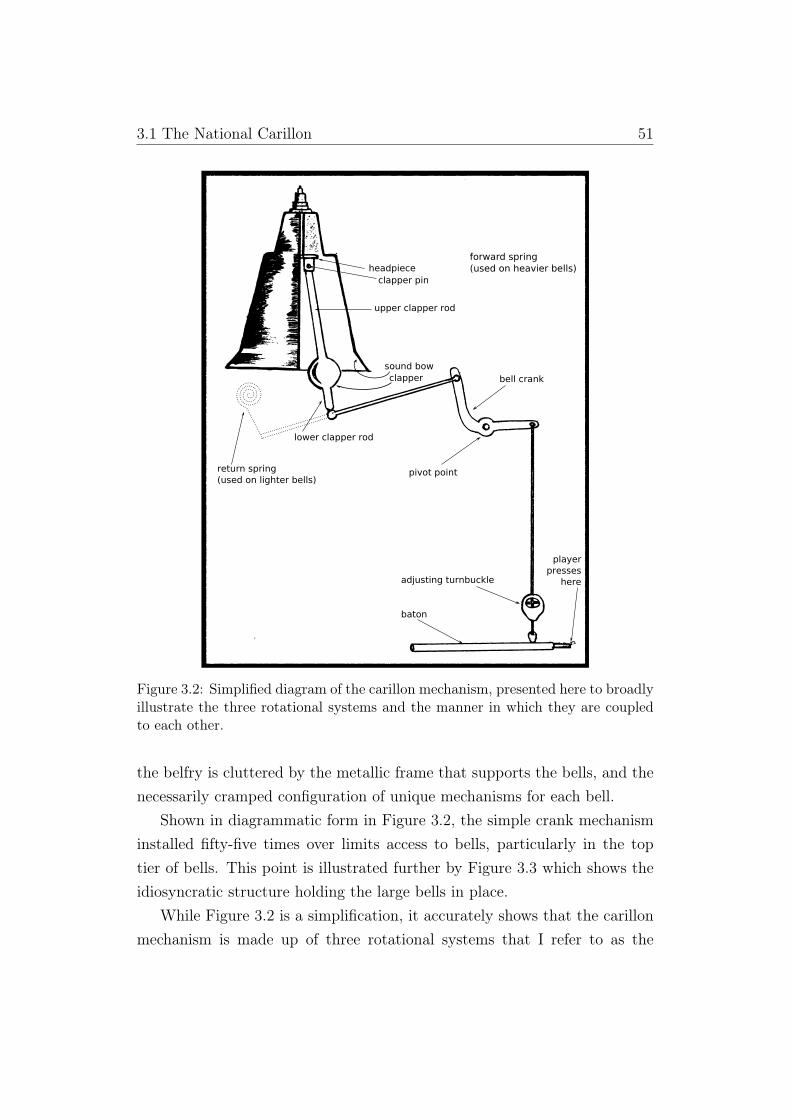
3.1 The National Carillon 51
forward spring(used on heavier bells)
Figure 3.2: Simplified diagram of the carillon mechanism, presented here to broadlyillustrate the three rotational systems and the manner in which they are coupledto each other.
the belfry is cluttered by the metallic frame that supports the bells, and thenecessarily cramped configuration of unique mechanisms for each bell.
Shown in diagrammatic form in Figure 3.2, the simple crank mechanisminstalled fifty-five times over limits access to bells, particularly in the toptier of bells. This point is illustrated further by Figure 3.3 which shows theidiosyncratic structure holding the large bells in place.
While Figure 3.2 is a simplification, it accurately shows that the carillonmechanism is made up of three rotational systems that I refer to as the

3.1 The National Carillon 52
Figure 3.3: View of 2nd and 3rd Tiers, National Carillon. From right: bell 21, 23and 25. Note the change in clapper shape from a sphere to a tear-drop.
clapper, crank and the baton systems.Although each carillon is different, it is possible to define a general model
for the construction, static and dynamic behaviour of modern carillons. Thisgeneral model takes the form of three rotational systems exchanging forcesthrough their linking cables. These forces are made up of the net torqueabout the pivot point for each system. This torque is mainly the product ofthe magnitude and distance from the pivot of masses in each system.
In its rest position, each baton rests against one of two felt-lined woodenbeams that run horizontally across the range of the clavier, the upper beamfor sharp and flat notes and the lower for natural notes; in this position, theclapper on each bell is held away from the inside rim of the bell. When aplayer presses downward on a baton, the clapper is pulled toward the insideshoulder of the bell. When the player applies no force, the baton moves backtoward the rest position as the clapper moves away from the bell, in a motiondetermined mainly by the dynamics of that clapper.

3.2 Modelling Strategy 53
Surprisingly, it is only in relatively few bells that the actual clapper massis responsible for most of what the carillonneur experiences as force-feedback.
In the lower bells and up to bell 24, forward springs assist the carillonneurin overcoming the gravitational potential of the clapper. From bell 34 up,return springs attached behind the clapper help pull the clapper away fromthe inside of the bell after impact and also generate an increasing force-feedback to the carillonneur. Without return springs on the highest bells,gravity acting on the baton’s mass will generate enough force to hold theclapper against the bell wall. The middle ten bells do not require springs.
3.2 Modelling Strategy
3.2.1 A Generalised Model Based on Bell 4, B0
In order to model the behaviour of the entire instrument, a single bell is firstmodelled to as high a degree of accuracy as possible, and this model is thengeneralised and fit it to other bells. Because the clapper mechanism cannot bedismantled for analysis, the model is constructed with a mix of measurementstaken onsite and calculations based on those measurements. A kinematicmodel is constructed based on these measurements and calculations, leadingto equations of motion that describe the natural motion of that bell.
The following analysis is based on the geometric and dynamical measure-ments taken of bell 4 (B0), the most easily accessible bell in the NationalCarillon. This bell features a forward spring to mitigate the effects of theclapper’s mass.
The baton is coupled to one arm of the crank at about half-way along thebaton’s length, giving the carillonneur a mechanical advantage of 2:1. Of thetwo arms that constitute the crank, the one that is coupled to the baton liesflat on the horizontal axis and the other arm — formed in an L-shape — iscoupled to the end of a rod that extrudes from the base of the clapper.
All couplings in this carillon are made with stiff, lightweight cable thatis a little slack prior to a stroke, but is taut when the force is applied to thebaton. Each coupling with the exception of the cable attached to the baton
3.3 The Clapper System 54
is an unconstrained revolute joint. When the coupling cables are taut thethree systems form a closed kinematic loop and are constrained to accelerateuniformly so the entire mechanism has only one degree of freedom. In morecomplex instances the three systems may each operate independently and thesystem exhibits greater degrees of freedom — these scenarios are discussedin the next chapter.
The angle made between the cables and the lever arm of their respectiverotating systems remains roughly perpendicular throughout operation. Thisfeature of the carillon’s design is later used to our advantage when linearisinga general mathematical model.
The turnbuckle, shown in Figure 3.2 allows a carillonneur to easily reg-ulate the length of the cable to the crank, which has the practical effect ofcalibrating the alignment of the baton’s range and the clapper’s range. Turn-buckle length is a surprisingly delicate variable, simulations in the followingchapter demonstrate its influence on the mechanism dynamics.
A full analysis of the National Carillon’s constituent parts follows whichis then used to develop precise equations of motion that are tested againstmeasurements taken of the individual rotational systems.
3.3 The Clapper System
The clapper system (Figure 3.4) is made up of three components that I shallcall the upper clapper rod, the clapper and the lower clapper rod. In theNational Carillon, bells 1–35 have a curved upper clapper rod whilst higherbells have a straight rod; the clapper shape is more spherical in higher bells,becoming fully spherical by bell 18; while the angle at which the lower clapperrod protrudes from the clapper remains fairly close to perpendicular over therange of the carillon.
The three components are welded together and therefore have only onedegree of freedom, that is rotation about a pivot point where the top of theupper clapper rod is attached to the top of the bell. In order to determineequations that describe the rotation of the clapper, we take an analyticalapproach to the geometry of the constituent parts, determine their geometric

3.3 The Clapper System 55
Figure 3.4: Computer-generated model of the clapper for bell 4 at rest. Note thecurvature of the upper clapper rod and the angle slightly less than 3π/2 of the rodat rest.
centroids and centres of mass, then sum them as point masses rotating aboutthe pivot point. Moments of inertia are also calculated to complete theequations of motion.
Analysis Notes
As the system moves only in the x/y plane, the depth of individual compo-nents is considered only in calculations to determine mass-related properties.Mass values are derived from the geometrical analysis and a density value ρfor cast iron of approximately 7300 kg/m3 [42].
The coordinate system for the clapper system is labelled CSclapper withan origin (Ox, Oy) defined as the point at which the upper clapper rod isattached to the revolute joint inside the bell — a small circular cut labelled

3.3 The Clapper System 56
in Figure 3.6.The centroids for the constituent parts are constrained to rotate uni-
formly about the point (Ox, Oy) and therefore dependant on the clapperangle θclapper. For visual simplicity all analysis is conducted with the systemnaturally oriented where θclapper = 3π/2.
The values θclapperminand θclappermax
respectively describe the clapper sys-tem’s orientation when the system is at rest and when in contact with thebell.
Forward Kinematics
When analysing each part, the coupling point/s and centre of mass (COM)are first determined in the coordinate system CSn for the part itself andrecorded as point vectors (xn, yn) and (xn, yn) for the coupling point andCOM respectively. These points are then used to form vectors rn and rCOMn
that are links in a kinematic chain that continues from the absolute locationof the previous part’s coupling point such that
rn =
[xnı
yn
]− pn−1 (3.1a)
and
rCOMn =
[xnı
yn
]− pn−1 (3.1b)
where pn−1 is the point in the local coordinate system CSn that is equal to thesame coupling point in the previous coordinate system CSn−1, (xn−1ı+yn−1).
Using forward kinematics, the absolute position of any point in CSclapperis then found by summing and transforming the respective local vectorsr1 . . . rn. The general form for this is:[
xnı
yn
]=
n∑i=1
0Ti(ϕi) . ri, (3.2a)

3.3 The Clapper System 57
where the transformation matrix from the coordinate frame of link n relativeto frame of link 0 is
0Tn =n∏i=1
i−1Ti(ϕi), (3.2b)
the absolute dot product of the transformation matrices i−1Ti which are them-selves functions of ϕi, the angle of link i relative to link i− 1.
The absolute position of any COM is found by a slight adjustment to theprevious equation[
xnı
yn
]=
(n−1∑i=1
0Ti(ϕi) . ri
)+0 Tn . rCOMn . (3.3)
Unlike vectors rn which represent a local frame’s link in the clapper’skinematic chain, COM vectors rCOMn are located in the CSclapper frame andare solved for this at the end of each subsection.
In this 2 dimensional case each transformation is limited to a single rota-tion of the form
Rotzi(ϕi) =
[cosϕi − sinϕi
sinϕi cosϕi
]. (3.4)
Figure 3.5 illustrates the relationships between position vectors and co-ordinate systems, and shows some important position vectors that are cal-culated and presented in the following sections. Note that the first rotationangle ϕ1 angle is dependant on θclapper, which is equal to 3π/2 when theclapper rod is in line with the negative y-axis. While θclapper does not itselfdirectly dictate the orientation of any particular vector it is a value uponwhich all vectors are dependant by virtue of their dependence on CSn and istherefore often included in a final value for position vectors throughout thissection.
Also, a note on labelling: the following sections will occasionally record apart’s centre of mass and coupling point in polar coordinates that are easilyimplemented in later dynamic equations as generalised coordinates. Thisnotation is also useful for comparing the dimensions of bell 4 to measurements

3.3 The Clapper System 58
x
-y
CS1
x
y
CS2
r1
r2
= θclapperφ
1
φ2
x
CS3φ3
y
x
-y
x
y
rcom
θclapper
x
y
rspring
rcrank
rcom1
rcom2
rcom3
Figure 3.5: Vector representation of clapper kinematics, including the location ofvectors rcom, rspring and rcrank which are listed in Table 3.1 and the centres of massfor the three parts, which are not.
taken of other bells in which length-wise dimensions were recorded but angleswere not.
3.3.1 Upper Clapper Rod
The upper clapper rod (Figure 3.6) is considered in two parts: the rectangularprism formed by l1 l2 and l3, and the arc of β radians formed by the sectorof radius r2 subtracted from the sector of radius r1.

3.3 The Clapper System 59
Figure 3.6: Upper clapper rod.
The rectangular prism has a mass
M1 = ρ(l1l2l3) (3.5)
and centroid(x1, y1) =
(x2− l2/2,
y
2
). (3.6)
The centroid for the arc lies on a straight line that bisects the arc from itsorigin at an angle β/2; to simplify analysis, the sector is rotated clockwise byβ/2 so that the centroid lies on the x axis. The centroid x2 is then determinedby dividing the weighted mass mean 〈x〉1−〈x〉2 by the total mass. The inner

3.3 The Clapper System 60
sector of radius r2 is then subtracted from the outer sector of radius r1.The mass of both arcs is calculated by solving the general double integral
for the mass of a sector
Mr1 =
∫ r1 sin(β/2)
−r1 sin(β/2)
∫ √r21−y2
|y|cot(β/2)
∫ l3
0
ρ dz dx dy
Mr1 =
∫ r2 sin(β/2)
−r2 sin(β/2)
∫ √r22−y2
|y|cot(β/2)
∫ l3
0
ρ dz dx dy (3.7)
M2 = Mr1 −Mr2 (3.8)
Values 〈x〉1 and 〈x〉2 are calculated
〈x〉1 =
∫ r1 sin(β/2)
−r1 sin(β/2)
∫ √r21−y2
|y|cot(β/2)
∫ l3
0
xρ dz dx dy
〈x〉2 =
∫ r2 sin(β/2)
−r2 sin(β/2)
∫ √r22−y2
|y|cot(β/2)
∫ l3
0
xρ dz dx dy, (3.9)
then divided by mass to find the centroid δ of this sector
δ =〈x〉1 − 〈x〉2
M2
. (3.10)
As this value is for a sector symmetrical about the x-axis, the actualcoordinates of the centroid are found by adding the origin of the arc [(r2 +
l2/2),−l1] and rotating back counter-clockwise β/2 while adding π to set thesign.
x2 =
(r2 +
l22
)+ δ cos
(β
2+ π
)(3.11)
y2 = −l1 + δ sin
(β
2+ π
)(3.12)
The mass and the centroid for the entire upper clapper rod is the weighted

3.3 The Clapper System 61
average of the two centroids in the system
m1 = M1 +M2 (3.13)
(xupperRod, yupperRod) =
2∑i=1
xiMi
2∑i=1
Mi
,
2∑i=1
yiMi
2∑i=1
Mi
(3.14)
which is converted to polar coordinates to simplify later rotation calculations
rupperRod =√x2upperRod + y2upperRod (3.15a)
θupperRod = π/2 + tan−1(yupperRodxupperRod
)+ θoff (3.15b)
where
θoff = ϕ1 = θclapper − (3π/2) (3.15c)
The relation θoff = ϕ1 is also used to establish the transformation func-tion for all points in the upper rod’s CS, taken from Eq. (3.4):
0T1 = Rotz(ϕ1) =
[cosϕ1 − sinϕ1
sinϕ1 cosϕ1
], (3.16)
and the upper rod’s centre of mass is found by applying this transform tothe point vector
rCOM1 = 0T1.
[xupperRodı
yupperRod
]. (3.17)
The vector r1 describes the point at which the upper clapper rod is welded

3.3 The Clapper System 62
to the clapper, the coordinates are also given in polar coordinates:
r1 =
[x1ı
y1
]
rupperRod =√x21 + y21
θupperRod = π/2 + tan−1(y1x1
)+ θoff (3.18)
where, labelled in Figure 3.6,
x1 =
(r2 +
l22
)(1− cos β)
y1 = −l1 +
(r2 +
l22
)sin(β + π). (3.19)
Plugging in the measured values for this upper clapper rod from bell 4 andsetting the clapper angle θclapper = 3π/2 gives the coordinates for the rod’scentroid at rest; the coordinates can then be transformed by the rotationangle θclapper. The centroid and all other values particular to bell 4 are listedin Table 3.1.
Moments of Inertia
The upper rod’s moment of inertia for rotation about the z axis at its centreof mass is
Icom =1
12M(l21 + l22). (3.20)
Applying the parallel axis rule, the moment of inertia about the pivot iscalculated as
Izz1 = Icom +Md2 (3.21)
where the pivot is a distance d away from the centre of mass.The curved portion at the bottom of the upper clapper rod can be consid-
ered part of a thick-walled hollow cylinder. The moment of inertia for such

3.3 The Clapper System 63
a cylinder about its axis of symmetry is
Izz =1
2M2(r
21 + r22), (3.22)
where r1 and r2 are the outer and inner wall radii respectively.Using the parallel axis rule the moment of inertia is found for the sector’s
centre of mass by subtracting the product of the mass and squared distanceto the centre of mass of the hypothetical cylinder. The product of the massand squared distance to (Ox, Oy) is then added to this, giving the momentof inertia about the upper clapper rod revolute joint
Izz2 = Izz −M2δ2 +M2(x
22 + y22), (3.23)
where δ, x2 and y2 were found in Eqs. (3.10–11).Summing Eq. (3.21) and Eq. (3.23) determines the moment of inertia for
the entire upper clapper rod about the z axis located at the revolute joint,(Ox, Oy).
IupperRod = Izz1 + Izz2 (3.24)
3.3.2 Clapper
The clapper is cast in a slightly different shape across the range of the carillon,changing from near cylindrical in bells 1-15 to a sphere in the lower-middlebells (visible in Figure 3.3) and an upright tear-drop shape in the middle-higher bells. The clapper for bell 4 is shown in Figure 3.7.
The clapper shape can be modelled by determining a function for thechange in radius over change in x, and this function yclapper(x) is integratedto determine both the mass and centroid for the shape; this is the disc methodfor determining the volume of a 3-dimensional shape of known radius that issymmetrical about one axis.
In the case of the clapper, the shape is symmetrical about the x axisand the change in radius is described by three continuous functions, γ1−3(x).γ1(x) and γ3(x) are the 2nd and 1st quadrants of a circle, respectively, andare solved for x using the general equation for a circle (x−h)2 +(y−k)2 = r2

3.3 The Clapper System 64
Figure 3.7: Photograph of the clapper for bell 4 at rest. The discoloured portionat the tip of the clapper is the damage flat.
where (h, k) are the x- and y-coordinates of the centre of the circle. γ2(x) issimply a sloped line.
The piecewise function Eq. (3.25) describes the clapper’s changing radiususing dimensions labelled in Figure 3.8. δ1−2 determine the change in widthof the clapper from left to right, l4−6 determine the dimensions along thex-axis, and r3−4 are reference lengths that determine the magnitude of theclapper’s curvature at its ends.
yclapper(x) =
γ1(x) if 0 < x ≤ l4
γ2(x) if l4 < x ≤ l5
γ3(x) if l5 < x ≤ l6
(3.25)

3.3 The Clapper System 65
∆1 r3
∆2r4
l4l5
l6
H0, 0L Ix-clapper, y-
clapperM
Hx1, y1L
x
y
Figure 3.8: Analytical model of the clapper for bell 4 as described in Eq. 3.25;dimensions as listed in Table 3.1. The clapper’s centre of mass (xclapper, yclapper)and the upper rod weld points (x1, y1) are also shown here.
The individual functions are
γ1(x) =√r23 − (x− r3)2 (3.26a)
γ2(x) =δ2 − δ1l5 − l4
(x− l4) + δ1 (3.26b)
γ3(x) =√r24 − (x− (l6 − r4))2 (3.26c)
Considering Figure 3.8 and the relationships in Eqs. (3.26a–c), the clap-per’s proportions obey the following constraints
δ1 =√r23 − (l4 − r3)2
δ2 =√r24 − (l5 − (l6 − r4))2 (3.27)
and these proportions can be manipulated by solving the above equations for
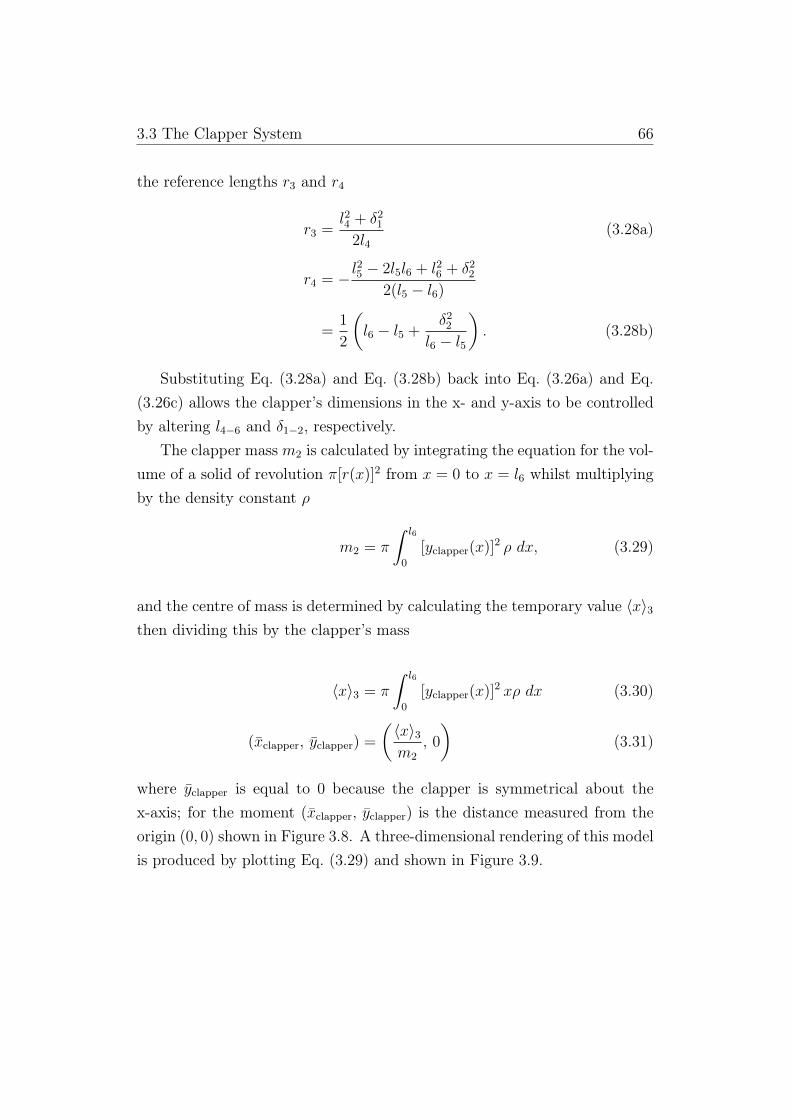
3.3 The Clapper System 66
the reference lengths r3 and r4
r3 =l24 + δ21
2l4(3.28a)
r4 = − l25 − 2l5l6 + l26 + δ22
2(l5 − l6)
=1
2
(l6 − l5 +
δ22l6 − l5
). (3.28b)
Substituting Eq. (3.28a) and Eq. (3.28b) back into Eq. (3.26a) and Eq.(3.26c) allows the clapper’s dimensions in the x- and y-axis to be controlledby altering l4−6 and δ1−2, respectively.
The clapper mass m2 is calculated by integrating the equation for the vol-ume of a solid of revolution π[r(x)]2 from x = 0 to x = l6 whilst multiplyingby the density constant ρ
m2 = π
∫ l6
0
[yclapper(x)]2 ρ dx, (3.29)
and the centre of mass is determined by calculating the temporary value 〈x〉3then dividing this by the clapper’s mass
〈x〉3 = π
∫ l6
0
[yclapper(x)]2 xρ dx (3.30)
(xclapper, yclapper) =
(〈x〉3m2
, 0
)(3.31)
where yclapper is equal to 0 because the clapper is symmetrical about thex-axis; for the moment (xclapper, yclapper) is the distance measured from theorigin (0, 0) shown in Figure 3.8. A three-dimensional rendering of this modelis produced by plotting Eq. (3.29) and shown in Figure 3.9.

3.3 The Clapper System 67
Figure 3.9: Three-dimensional rendering of clapper model; this shape is easilymanipulated by adjusting the values in Eqs. (3.26a–c). The points at which theclapper is welded to the upper and lower clapper rods are also shown.
Coupling to Upper and Lower Clapper Rod
The location of the clapper’s centre of mass with respect to the revolute jointof the upper clapper rod is calculated in two steps:
1. Manipulate this coordinate system CS2 such that the point (x1, y1) isequal to (r3, yclapper[r3]) in CS2 (Figure 3.8), and equal to that samepoint (x1, y1) (Figure 3.6) on the upper rod in the previous coordinatesystem CS1, described by Eqs. (3.18–19); and
2. Assume that a line tangent to the sector [β (r1−r2)] at (x1, y1) (Figure3.6) is perpendicular to the clapper’s x-axis (slightly difficult to recog-nise in the photograph but clearer in Figure 3.9) and transform CS2
anti-clockwise by ϕ2 to orient it correctly.

3.3 The Clapper System 68
We find the coordinates of the clapper’s centre of mass with respect tothe weld point instead of CS2’s origin then add and transform this to theabsolute position of this weld point represented by r1; the value rCOM2 thencorresponds to the location of the clapper’s centre of mass in the coordinatesystem CSclapper.
From Eq. (3.2b) and Eq. (3.3):
rCOM2 = 0T1.r1 + 0T2.
[(xclapper − x1)ı(yclapper − y1)
](3.32)
where
(x1, y1) = (r3, yclapper[r3])
1T2 = Rotz(ϕ2) =
[cosϕ2 − sinϕ2
sinϕ2 cosϕ2
](3.33)
andϕ2 = β − θupperRod. (3.34)
Following on from the second step, the gradient of the line tangent to βis assumed to continue through the clapper to the point at which the lowerclapper rod protrudes and continues in a straight line parallel to the y axisin the local coordinate system, so
r2 =
[(r3 − r3)ı
(−2yclapper(r3))
]. (3.35)
The clapper’s centre of mass in polar coordinates in the CSclapper is:
rclapper =√r2COM2x
+ r2COM2y(3.36a)
θclapper = π/2 + tan−1rCOM2y
rCOM2x
(3.36b)

3.3 The Clapper System 69
Moment of Inertia
The clapper’s moment of inertia about the about the origin of the localcoordinate system — the leftmost point of the clapper — is calculated usingthe triple integral
Izzend = ρ
∫ l6
0
∫ yclapper(x)
−yclapper(x)
∫ √yclapper(x)2−y2
−√yclapper(x)2−y2
(x2 + y2) dz dy dx, (3.37)
The parallel axis rule is then used to adjust this for the clapper’s centre ofmass, then the revolute joint of the upper clapper rod.
Izzcom = Izzend −m2x2clapper (3.38a)
Iclapper = Izzcom +m2||rCOM2||2. (3.38b)
3.3.3 Lower Clapper Rod
The lower clapper rod is a rectangular prism that protrudes from the bottomof the clapper in a perceivable continuation of the the upper clapper rod.It features three small circular cuts that couple the the clapper system to aspring, the crank, and a rubber damper that stops the clapper moving morethan a small distance away from the inside of the bell.
The mass m3 and the centre of mass (xlowerRod, ylowerRod) are determinedas for the upper rod in §3.3.1
(xlowerRod, ylowerRod) =
(l22,l102
)(3.39)
m3 = ρ(l2l3l10) (3.40)
The centre of mass is then determined as a point in the CSclapper coordi-nate system, with respect to the upper clapper rod revolute joint, as in Eq.

3.3 The Clapper System 70
Figure 3.10: Lower clapper rod. The point at which the rod is welded to theclapper is indicated by (x2, y2).
(3.32) and Eq. (3.33), and described in general form in Eq. (3.3)
rCOM3 =2∑i=1
0Ti.ri +0 T3.
[(xlowerRod − l11/2)ı
−ylowerRod
](3.41)
where the transformation matrix
2T3 = Rotz(ϕ3) =
[cosϕ3 − sinϕ3
sinϕ3 cosϕ3
](3.42)
is equal to no transformation because ϕ3 = 0.
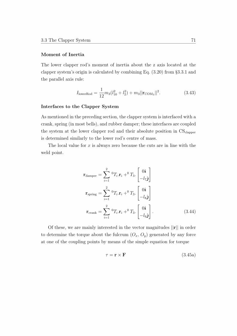
3.3 The Clapper System 71
Moment of Inertia
The lower clapper rod’s moment of inertia about the z axis located at theclapper system’s origin is calculated by combining Eq. (3.20) from §3.3.1 andthe parallel axis rule:
IlowerRod =1
12m3(l
210 + l22) +m3||rCOM3||2. (3.43)
Interfaces to the Clapper System
As mentioned in the preceding section, the clapper system is interfaced with acrank, spring (in most bells), and rubber damper; these interfaces are coupledthe system at the lower clapper rod and their absolute position in CSclapperis determined similarly to the lower rod’s centre of mass.
The local value for x is always zero because the cuts are in line with theweld point.
rdamper =2∑i=1
0Ti.ri +0 T3.
[0ı
−l7
]
rspring =2∑i=1
0Ti.ri +0 T3.
[0ı
−l8
]
rcrank =2∑i=1
0Ti.ri +0 T3.
[0ı
−l9
]. (3.44)
Of these, we are mainly interested in the vector magnitudes ||r|| in orderto determine the torque about the fulcrum (Ox, Oy) generated by any forceat one of the coupling points by means of the simple equation for torque
τ = r× F (3.45a)

3.3 The Clapper System 72
or
τ = rF sin θ, (3.45b)
where r is the distance from the point at which the magnitude of a force Fis applied at an angle θ.
Of the three interfaces we only have enough information to determine θfor the cable to the crank — this is shown during analysis of the linkagein §3.7. The connection angle to the spring, while changing as the clapperrotates, does not deviate too much from π/2 and is modelled as permanentlyequal to that.
The connection length and angle to the rubber damper is ignored becausethe damper’s influence on clapper rotation is determined empirically, by ob-serving the clapper’s motion after impact with the damper, so it is applieddirectly as torque to the fulcrum. This is described further in Chapter 4.
3.3.4 The Spring
As mentioned in earlier sections, the role of springs in the carillon mechanismis two-fold, and can be considered according to statics/dynamics.
• (Statics) Smooth and manage the force required from a carillonneuracross the range of the carillon without requiring dramatic adjustmentsto the each mechanism; adjusting springs is preferable to altering cranklengths as a means of managing the player’s mechanical advantage.
• (Dynamics) Tune the responsiveness of respective bell mechanisms;shown in a later section, bells low–high exhibit remarkably similar nat-ural motion. In higher bells return springs are used to pull the clapperaway from the bell after impact, the mass of the clapper alone insuffi-cient to overcome forces in the rest of the mechanism.
Bell 4 features a forward spring that helps the carillonneur pull the clappertoward the inside of the bell. In the National Carillon all the springs in the

3.3 The Clapper System 73
belfry are flat spiral springs, sometimes called brush springs.2 A large springused in one of the low bells is shown in Figure 3.11.
Figure 3.11: One of the largest flat spiral springs used in the carillon. It is mountedto the belfry frame with the bolt in the centre of the coil.
Smaller versions of the flat spiral spring are typical in clockwork mecha-nisms because they combine a compact and accurate means of storing energyand are easily ‘wound up’. In this scenario the centre of the spring is coupledto a pivot joint and is pinned as its outermost point; potential energy is thenstored in the spring by applying a torque at the pivot. The restoring torqueis described by the rotational form of Hooke’s law
τ = −kθ (3.46)
and like most springs is linear within its operational range. Springs in thecarillon operate under the same principle but potential energy is stored byforce applied at the outermost point — in Figure 3.11 this is where a thinrod is connected to the spring coil — which produces torque about the centreof the coil where it is pinned to the belfry structure.
In bells 1–21 only five different springs sizes are used. Their influence onthe mechanism is fine-tuned by adjusting the angle at which they are mountedand occasionally employing them in series, as in bell 4 (Figure 3.12).
2Helical torsional springs are used to tune the responsiveness of pedal mechanisms inthe clavier.

3.3 The Clapper System 74
This figure shows that the springs are coupled to the clapper system bya protruding arm the length of which is 10 cm here but varies dependingon the spring; a thin cable forming an angle ϕspring ≈ π/2 with the leverarm of length ||rspring|| and the same angle with the arm attached to thefirst spring’s outermost point. This angle changes only very slightly overthe clapper’s range of motion and is modelled as constant, ϕspring = π/2.Another cable couples the first spring to the second.
Figure 3.12: Three couplings to the clapper for bell 4. One of two flat spiral springsin series can be seen coupled to the middle cut in the lower clapper rod. The cablefrom the spring is not perpendicular to the rod itself, but is approximately so tothe lever arm rspring.
The theoretical determination of a flat spiral spring’s k requires that thematerial, thickness, length and spiral spacing be known. We do not know forcertain the material for even the most accessible spring in the carillon whereits length and geometry might be measured, so a theoretical determination isnot possible. Further, in the context of the spring’s coupling to the clappersystem we are less interested in the change in restoring torque than we arein the change in force the spring applies to the clapper system at the pointson the lower clapper rod rspring as the clapper system rotates from θclappermin
to θclappermax.

3.3 The Clapper System 75
This is measured by observing the point at which the cable is coupledto the spring; the absolute coordinates of this point are recorded when theclapper is at θclappermax
and again with the clapper at θclappermin. The clapper
is then uncoupled from the spring, and force measurements Fmax and Fmin aretaken for the spring at both of these displacements. Note that the max andmin subscripts relate to the clapper displacement, not the force magnitude.
Assuming a linear change in force we can then determine:
k =Fmax − Fmin
∆θclapper.
It is typical that neither Fmax or Fmin are equal to zero, so it is convenientto encapsulate this force offset by determining the angle, θs0 , at which thespring exerts no force:
(θS0 − θclappermax)k − Fmax = 0
θS0 =kθclappermax
− Fmax
k(3.47)
which can now be used in a universal expression for spring force acting onany clapper:
F = (θS0 − θclapper)k (3.48)
which must be converted to torque through multiplication by the distance||rspring||.
This final expression can be determined by measuring the spring’s restora-tion force at the clapper’s maximum and minimum rotations alone; theserelationships greatly simplify later parameter estimation.
3.3.5 Clapper System Values
Table 3.1 lists the recorded and calculated values for bell 4 that have beenused in the preceding calculations; these values are used to find a numericalsolution and simulate the free motion of the clapper system for bell 4 inChapter 4. In addition to these values, the moments of inertia for the entire

3.3 The Clapper System 76
Table 3.1: Clapper system parameters and calculated values.
Clapper SystemParameter Value
I1 69.25 kg·m2
I1com 5.14 kg·m2
mall 61.38 kgrcom (1.022 m, 10.78 ◦ + θclapper)rspring (1.34 m, 15.72 ◦ + θclapper)rcrank (1.41 m, 16.97 ◦ + θclapper)
Part
Upper Clapper Rod l1 0.705 ml2 0.064 ml3 0.023 mr1 0.47 mr2 0.406 mm1 11.52 kgIupperRod 3.98 kg·m2
β 48 ◦
Clapper l4 0.042 ml5 0.24 ml6 0.305 mδ1 0.105 mδ2 0.08 mm2 47.17 kgIclapper 59.18 kg·m2
Lower Clapper Rod l7 0.075 ml8 0.15 ml9 0.225 ml10 0.25 mm3 2.69 kgIlowerRod 6.09 kg·m2
Forward Spring k -193 N/radθS0 297.24 ◦Fmin 85 NFmax 70 N
system rotating about the origin, I1, and its centre of mass, I1com , are listed.The vectors describing the location of the clapper system’s centre of mass,

3.4 The Crank System 77
the spring coupling and the crank coupling are also listed in polar coordinaterepresentation for linkage analysis in section §3.7.
3.4 The Crank System
The crank mechanism converts the near-vertical motion of the baton to near-horizontal motion that pulls the clapper toward the inside of the bell wall.It consists of a thin rod that links the baton, an L-shaped rod called theclapper fly that links to the lower clapper rod, and a rotating shaft that ismounted at both ends to the a bearing housing attached to the belfry frame.The crank rods are coupled to the shaft by means of a thin ring that is eitherscrewed or welded to the shaft.
Like the clapper system, the precise dimensions of the crank system varyover the carillon. Indeed, cranks in the National Carillon bear evidence ofhaving been used for different bells at different times, and now-unused rodsare still welded to their shafts. The crank system for bell 4 presented herefeatures no remnants from use on another bell and is in the larger of twogroups of crank systems; the group of cranks in bells 28 and higher arelighter and have a slightly smaller clapper fly.
Figures 3.13 and 3.14 show the crank’s orientation in the rest position,when the baton is resting against the upper beam at the clavier, and theclapper is away from the inside of the bell. For dynamics we are interestedin the vectors rclapper and rbaton that contribute to the mechanical advantageof the player over the clapper, and the centres of mass of the rods to theclapper and baton, rCOMclapper and rCOMbaton . All values are determined withrespect to the origin (Ox, Oy) at the centre of the shaft.
These calculations are simplified by taking advantage of a natural oppor-tunity in the geometry of the crank: visible in Figures 3.13, when the entiresystem is in rest position the right crank rod which leads to the baton liesdirectly on the positive x-axis, and when the system is fully displaced —i.e. the clapper is in contact with the inside of the bell — the base of theL-shaped rod lies directly on the negative x-axis.
At all times, the angle θcrank describes the clockwise angle formed between

3.4 The Crank System 78
(a) Crank assembly, front view rest position.
rclapper
rbaton
y
x-x
β‐
(b) Crank assembly, front view away from rest position.
Figure 3.13: Crank assembly, in rest and pulled away positions.
the positive x-axis and the baton rod, as in Figure 3.13b; θcrankmin = 0 = 2π.This is intuitive because it forms a direct reference to the absolute rotationaldisplacement of crank system.
Lengths l2 and l4 are taken from the centre of the shaft to the end ofeach rod, as are the vector measurements. When determining mass based onthese lengths, the extension is a satisfactory estimate of the additional massintroduced by the ring or weld between each rod and the shaft.
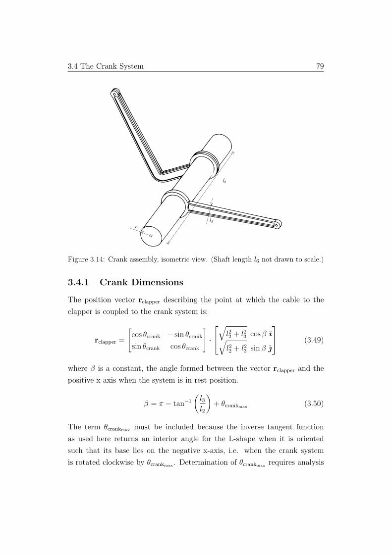
3.4 The Crank System 79
r1
l5
l6
Figure 3.14: Crank assembly, isometric view. (Shaft length l6 not drawn to scale.)
3.4.1 Crank Dimensions
The position vector rclapper describing the point at which the cable to theclapper is coupled to the crank system is:
rclapper =
[cos θcrank − sin θcrank
sin θcrank cos θcrank
]·
√l22 + l23 cos β ı√l22 + l23 sin β
(3.49)
where β is a constant, the angle formed between the vector rclapper and thepositive x axis when the system is in rest position.
β = π − tan−1(l3l2
)+ θcrankmax (3.50)
The term θcrankmax must be included because the inverse tangent functionas used here returns an interior angle for the L-shape when it is orientedsuch that its base lies on the negative x-axis, i.e. when the crank systemis rotated clockwise by θcrankmax . Determination of θcrankmax requires analysis

3.4 The Crank System 80
of the kinematics of the baton system because rotation of the crank shaftis constrained by clavier properties, and is different for sharp and naturalbatons. This is solved in §3.6.
It is important to note, but not dwell on the fact that the constant βis not usually the same for any two crank mechanisms in this carillon; mostother cranks have a larger β value. Hurd explains that the carillon installer ordesigner adjusts the offset angle of the clapper fly to refine the carillonneur’sexperience of a particular bell:
The ‘bell-cranks’ that transfer the vertical key motion to hor-izontal direction to move the clappers, as well as the clapper ends(a.k.a. clapper ‘flights’) can be made with multiple cross-holes topermit some adjustment of applied forces. In the best scenario,the bell-cranks and clapper flights would be round section withsome kind of sleeve collar arrangement, so that the actual clappertravel from rest to strike can be carefully adjusted, relative to theconstant vertical travel of manual keys. Upon installation, thebell-cranks can also be locked/set on the round transmission barat different angles to achieve desired applied force and clappertravel.
In large carillons, the clapper travel should be about 70–75%of vertical travel for the largest bells, gradually increasing to a 1:1(100%) ratio in the mid-range, then going up to about 115% forthe smallest treble bells — all this to help balance the instrumentacoustically. I know of a couple of carillons that use a directcable transmission with single slotted rollers and which have a1:1 force ratio across the entire range = these are truly miserableinstruments to play and control, because the bass bells are wayheavy and the trebles sound anaemic because they need a largerclapper travel than this. (Personal communication, November 23,2009)
Unlike rclapper which is offset by a variable β the vector rbaton is orientedthe same across the entire carillon, and is described by:

3.4 The Crank System 81
rbaton =
[cosϕbaton − sinϕbaton
sinϕbaton cosϕbaton
]·
[l4 ı
0
]
ϕbaton = 2π − θcrank. (3.51)
The masses and centres of mass for objects in the crank system are cal-culated as in the previous section.
xclapper =
mclapper1l22
+mclapper2
(l2 −
l12
)mclapper
yclapper =mclapper2
l3 − l12
mclapper, (3.52)
where
mclapper = mclapper1 +mclapper2
mclapper1 = ρ(l1l2l5)
mclapper2 = ρ(l1l5[l3 − l1])
mbaton = ρ(l4l1l5) (3.53)
Then including the angle θcrank the centres of mass are fully described by
rCOMbaton =
[cosϕbaton − sinϕbaton
sinϕbaton cosϕbaton
]·
[l4/2 ı
0
](3.54)
and
rCOMclapper =
[cosϕCOMclapper − sinϕCOMclapper
sinϕCOMclapper cosϕCOMclapper
]·
√x2clapper + y2clapper ı
0
(3.55)
where ϕCOMclapper is solved as in Eq. (3.50) because it is determined when the

3.4 The Crank System 82
crank is oriented such that θcrank = θcrankmax
ϕCOMclapper = (π − tan−1(yclapperxclapper
)+ θcrankmax)− θcrank.
The mass of the shaft is simply
mshaft = πr21l6ρ. (3.56)
The centre of mass of the crank system is calculated as
rCOM = rCOMclappermclapper + rCOMbatonmbaton (3.57)
and is listed in polar form in Table 3.2 at the end of this section.The moment of inertia for the entire crank mechanism about its pivot
point isIcrank = I1 + I2 + I3 (3.58)
where the moments of inertia for the L-shape rod I1, the rod to the batonI2, and the shaft I3 are
I1 = I11 + I12
I2 =1
12mbaton(4l24 + l21)
I3 =1
2mshaftr
21
I11 =1
12mclapper1(4l
22 + l21)
I12 =1
12mclapper2(l
23 + l21) +mclapper2((l2 − l1/2)2 + (l3/2)2). (3.59)
3.4.2 Crank System Values
The table below lists the values for cranks across the range of the carillondivided, as at the National Carillon, into those for bells 1–26 and slightlysmaller for bells 27–55.

3.5 The Baton System 83
The moment of inertia Icrank is for the entire crank system as it rotatesabout the shaft rather than about its centre of mass. The centre of mass forthe entire crank mechanism is also listed here for convenience.
Table 3.2: Crank system parameters and calculated values.
Crank System ## < 27 # ≥ 27
Parameter Values
rCOM (4.7 cm, 68.78 ◦) (4.6 cm, 71.07 ◦)m2 1.19 kg 0.79 kgmclapper 0.66 kg 0.44 kgmbaton 0.53 kg 0.35 kgI2 0.063 kg·m2 0.054·m2
l1 3 cm 2 cml2 7.25 cm 7.25 cml3 26 cm 25 cml4 24 cm 24 cml5 1 cm 1 cml6 2.28 m 2.28 mr1 3.5 cm 3.5 cmβ 113.95 ◦ 114.54 ◦
θcrankmaxN8.37 ◦ 8.37 ◦
θcrankmaxS7.76 ◦ 7.76 ◦
||rclapper|| 27 cm 26 cm||rbaton|| 24 cm 24 cm
3.5 The Baton System
The baton system is the place in the design of the carillon where the finesttweaks are made to manipulate the performer experience. TheWorld Carillonspecifications are precise in the dimensions and placement of components thatthe player actually touches; parts the player does not directly interact withare generally left up to the designer.
The wooden baton rotates about a pivot point its entire length away fromwhere the user applies force. It is in the shape of a rectangular prism for its

3.5 The Baton System 84
Figure 3.15: Baton assembly. The scale is that for sharp manual key; only one ofthe columns that fix a baton on either side is shown here. Notice that the cylinderintrudes slightly into the playing area of the sharp manual keys.
entire length except for the portion termed the playing length at the player’send, where it transitions from a square to conical cross-section and avoidssharp edges at the player’s point of contact.
At almost precisely half-way between the playing end and the pivot point,an aluminium flexure is attached to the baton, coupling it to a thin metal rodthat is then connected to a cable that attaches at its other end to the crank.The flexure is a relatively modern innovation, replacing standard hinges; byflexing back and forth it accommodates the baton’s slight rotational motionand allows the metal rod to move in vertical translation.
Apart from the actual shape of the wooden baton, the key dimensionalrelationships at the playing portion of the baton system are the length l5 —the projection length — and the keyfall distance measured at the face of thekey spreader where the aluminium cylinder marks the start of the projectionlength, l5; this is given by the continuous function
total keyfall↓y =
∫ θtop
−θbottom
(l1 − l5) cos θ dθ (3.60)
3.5 The Baton System 85
where θtop describes the baton’s angle in rest position, measured counter-clockwise from the positive x-axis, and θbottom the clockwise angle from thesame axis of the baton when fully displaced from the rest position. The totalangular displacement is then:
θtotal = θtop + θbottom. (3.61)
The technical standards laid out by the World Carillon Federation [31]leave some decisions to the individual carillon designer, but are very clear ona few particular items, specifying them to within a millimetre:
• a different projection length (l5) for natural and sharp keys;
• an equal and precise playing length for natural and sharp keys;
• change in diameter for cylindrical playing end at tip (from 20–16mm);
• vertical distance between the natural and sharp keys;
• horizontal spacing between keys; and
• that the (variable) keyfall be measured at the key spreader, not batontip and equal for sharp and natural keys
as well as several instructions regarding the arrangement of the pedals thatwe are not concerned with here.
This specificity is motivated by a desire to minimise the difficulties forconcert carillonneurs that have to perform with little notice on different in-struments. More interesting from an analytical standpoint than the dimen-sions that are specified so exactly, however, are those where the designer ispermitted or encouraged to exercise discretion; from the specifications, thefollowing are only suggested values or omitted entirely:
• both natural and sharp baton total lengths (l1);
• equal total keyfall measured at key spreader (constrained to between40 and 55 mm);

3.5 The Baton System 86
• total angular displacement, θtop and θbottom; and
• the distance from the tip of the playing end to the attachment pointfor vertical transmission wire (l1 − l2).
These values share the distinction of determining the mechanical advan-tage to the player over the rest of the carillon system and they are also someof the trickiest for the carillon installer to determine. Alongside the specifi-cations listed above are further constraints that relate to playability whichmust guide the installer.
A problem for carillon designers is that the the total keyfall measured atthe key spreader should be equal for natural and sharp keys, and that theflexures coupling the baton to the vertical transmission cable going up intothe bell tower must all lie on the same plane.3
However, because the projected lengths (l5) are different baton totallengths (l1) must also be adjusted in order to retain an equal mechanicaladvantage, and from Eq. (3.60) we see that their respective rotational limitsmust also be different. These constraints mean that only one of the followingtwo conditions can be met:
1. An equal mechanical advantage (l1 : l2) for natural and sharp batons;or
2. Equal vertical displacement at the transmission cable for natural andsharp batons.
3.5.1 Baton Keyfall and Mechanical Advantage
Keyfalls
Intuitively, this paradox is clear when stepped through. If both batons areinitially the same length and are mounted on the same keytail hinge, on thesame plane, then they have an equal mechanical advantage and an equalkeyfall at the key face — their total rotation is also equal. The transmission
3That is, for most carillons. In conversation with Hurd again he notes that some Dutchfounders continue to use two separate transmission planes for natural and sharp keys.
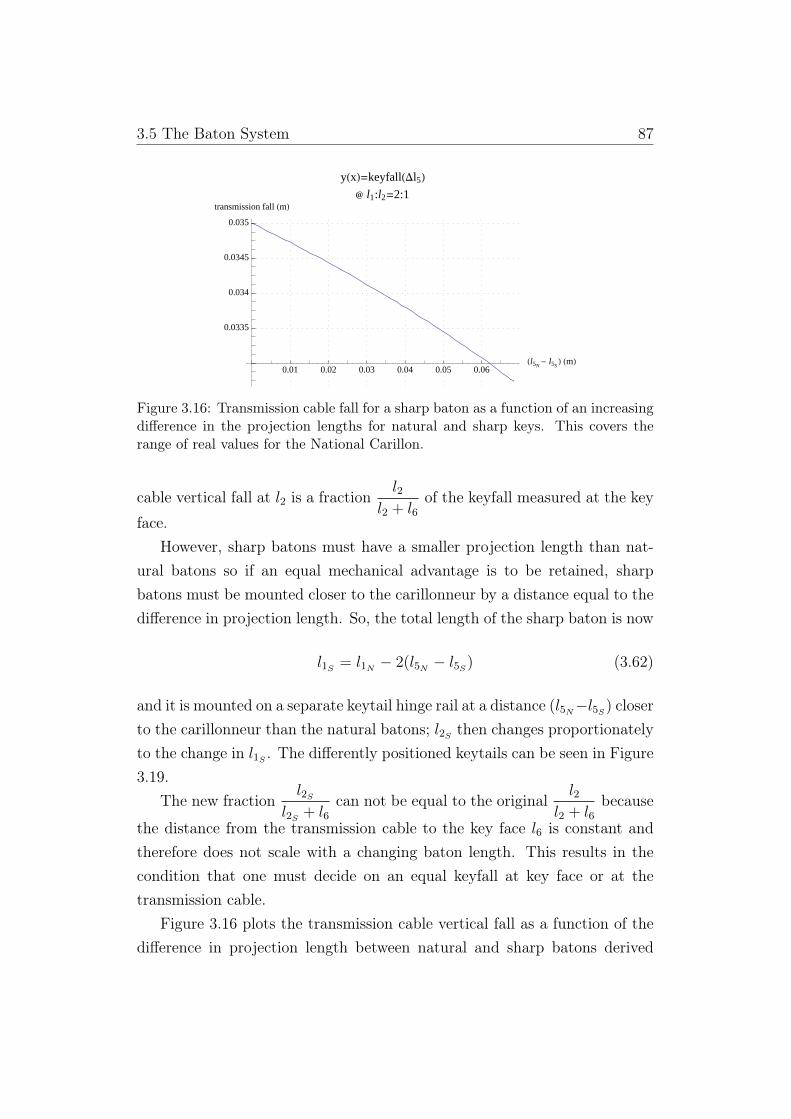
3.5 The Baton System 87
0.01 0.02 0.03 0.04 0.05 0.06Hl5N
- l5SL HmL
0.0335
0.034
0.0345
0.035
transmission fall HmL
yHxL=keyfallHDl5L� l1:l2=2:1
Figure 3.16: Transmission cable fall for a sharp baton as a function of an increasingdifference in the projection lengths for natural and sharp keys. This covers therange of real values for the National Carillon.
cable vertical fall at l2 is a fractionl2
l2 + l6of the keyfall measured at the key
face.However, sharp batons must have a smaller projection length than nat-
ural batons so if an equal mechanical advantage is to be retained, sharpbatons must be mounted closer to the carillonneur by a distance equal to thedifference in projection length. So, the total length of the sharp baton is now
l1S = l1N − 2(l5N − l5S) (3.62)
and it is mounted on a separate keytail hinge rail at a distance (l5N−l5S) closerto the carillonneur than the natural batons; l2S then changes proportionatelyto the change in l1S . The differently positioned keytails can be seen in Figure3.19.
The new fractionl2S
l2S + l6can not be equal to the original
l2l2 + l6
because
the distance from the transmission cable to the key face l6 is constant andtherefore does not scale with a changing baton length. This results in thecondition that one must decide on an equal keyfall at key face or at thetransmission cable.
Figure 3.16 plots the transmission cable vertical fall as a function of thedifference in projection length between natural and sharp batons derived

3.5 The Baton System 88
0.01 0.02 0.03 0.04 0.05 0.06Hl5N
- l5SLHmL
7.25
7.75
8.
8.25
8.5
8.75
total rotation H°LΘtotalHDl5L
Figure 3.17: Change in total baton rotation as a function of an increasing differencein the projection length for natural and sharp keys. As in the previous figure, thiscovers the range of real values for the National Carillon.
from the above relationship and the keyfall from Eq. (3.60):
tfall↓y = keyfall↓y ·(
l2Sl2S + l6
)(3.63)
where l2S =lS2, the projection lengths are initially equal (l5N − l5S) = 0, and
the sharp baton decreases in length to match its real-world value.Figure 3.17 plots the total angular range for a sharp baton as a function of
the difference in projection length between natural and sharp batons, derivedfrom the same relationships as above and defined by:
θtotal = sin−1(keyfall↓yl6 + l2S
). (3.64)
Mathematically, there is no solution to the following system of simulta-neous equations which describe the mechanical advantage, transmission wire

3.5 The Baton System 89
vertical travel and keyfall at the key face, respectively:
l2Nl1N
=l2Sl1S, (3.65a)
∫ θtopN
θbottomN
l2N cos θ dθ =
∫ θtopS
θbottomS
l2S cos θ dθ (3.65b)
∫ θtopN
θbottomN
(l1N − l5N ) cos θ dθ =
∫ θtopS
θbottomS
(l1S − l5S) cos θ dθ (3.65c)
where l5N 6= l5S because natural keys protrude further from the clavier frontthan sharp keys.4
However, if keyfall is measured at the baton tip, so Eq. (3.65c) is removedfrom the above set of equations and replaced with∫ θtopN
θbottomN
l1N cos θ dθ =
∫ θtopS
θbottomS
l1S cos θ dθ (3.66)
there are many possible solutions. So, why not mandate equal keyfall atthe key tip, and achieve an equal transmission cable fall and mechanicaladvantage for natural and sharp keys?
Carillonneur perception: As the carillonneur sits to face and play theclavier, the primary point of reference for the position of a baton is not itstip but the start of the projection length relative to the fixed columns thatconstitute the key face. Further, as typically half of the batons are doubled byfoot pedals and carillonneurs rarely play the lowest twenty bells by hand theyrely on this visual reference, particularly in the early stages of familiarisationwith a new instrument. Above all, the carillonneur is controlling the velocityof the clapper as it hits the bell; from their perspective at the front of theclavier the physical limits at the key face are the best guide to the clapper’sproximity to the bell.
Like all performers, carillonneurs maintain internal ‘targets’ for where todirect energy — the keyface limits are this point for carillonneurs. Figures
4Other than the trivial arrangement where the transmission cables are coupled to ba-tons at the keyface.

3.5 The Baton System 90
3.18b and 3.18c are taken from the discussion on chord-playing technique in[57] where the author advices students to “play into the instrument” as ameans of encouraging players to direct energy toward the end of the stroke;carillon instructors universally assert that a player should be in contact withand, using their natural weight, leaning into the baton prior to applying aplaying force. As well as avoiding significant backlash in transmission cablesand overcoming initial friction and some mechanical inertia this techniquehelps ensure a smooth velocity gradient through the stroke with the batonattaining the desired velocity at the end of the stroke.
A further explanation concerns the ease with which the carillonneur movesbetween the top and bottom banks of keys and plays chord intervals usingboth rows, in what is called ‘open hand position’. In conversation, Hurddiscusses a clavier design by Jef Denyn — as built by his colleague DesireSomers — where the key fall for black keys was drastically smaller than forwhite keys:
. . . [this design] made playing chord intervals across upper andlower key banks (with open hand position) nearly impossible asregards simultaneous striking at the bottom of the two key banks.It also severely/adversely affected rhythmic accuracy in fast pas-sage work involving both white and blacks (chromatic scales, forexample).
This depiction of the problems with unequal keyfall buttresses the percep-tion argument, and also provides the simple geometric argument that settingan equal keyfall at the key face is the closest a clavier designer can achieve toa comfortable progression from the larger keyfall at the tip for natural keysto the smaller keyfall at the tip of sharp keys. That is, as the carillonneur’sabsolute hand position nears the key face, the keyfall for both batons ap-proaches equality and in an open hand position the difference in keyfalls atthe hand’s absolute location (i.e. near the start of the playing length l5 fornatural batons and approximately half-way into the sharp baton’s playinglength) is close to negligible. Figure 3.18a shows the change in difference forbaton key falls as the player’s absolute position nears the keyface.

3.5 The Baton System 91
(a) Baton keyfall as a function of hand distance from keyface (x-axisto scale; y-axis is not). In this image, the thumb on the natural keywill fall 6.5 cm, and the index finger on the sharp key will fall thesame distance.
(b) Open chord position withthumb on lower row.
(c) Open chord position withthumb on upper row.
Figure 3.18: Hand positions relative to baton key fall distances.
Visualising the two open hand positions against the plot for baton key-fall one observes the maximum difference in keyfall to be around 1/4 of acentimetre for the position shown in Figure 3.18b and close to zero for theposition shown in the Figure 3.18c. Note that whilst the first position isshown here with the thumb near the tip of the natural key it can easily beplayed with the thumb further inward, closer to the finger alignment of thesecond position; the hand in the second position, however, can not be rotatedsuch that the fingers are set further away from the keyface.
This indicates that the optimal arrangement for an equal keyfall is for the

3.5 The Baton System 92
fingers on a natural key to be set a small distance back from the fingers ona sharp key: Figure 3.18a shows that for a hand position where one or manyfingers are on a sharp baton the difference in keyfall is minimised when theother fingers are 1.5 centimetres further away from the keyface. By contrast,were keyfall equal at the baton tip this distance increases to closer to 5centimetres.
The reasons above are compelling ones for mandating keyfall to be equalat the keyface, returning us to the problem of an unequal transmission fall ifan equal mechanical advantage is to be maintained.
Mechanical Advantage — Transmission Cable Placement and Fall
Solving for mechanical advantages using the measured values shows a 2:1ratio to the player:
l2N/l1N ≈ l2S/l1S ≈ 0.5 (3.67)
The National Carillon designer has clearly chosen an equal mechanicaladvantage which means the transmission cable fall for natural and sharpkeys is different; Figure 3.16 shows the difference to be close to 0.25 cm withnatural and sharp transmission cables falling 3.5 and 3.27 cm, respectively.This difference in transmission cable travel translates to a difference in totalclapper travel — again, with sharp clappers rotating over a smaller distancethan natural clappers. Aside from the tautological equality in torque ad-vantage over the rest of the carillon mechanism, maintaining an equal ratio(l1 : l2) helps the carillonneur develop a sense of the slighter rotation of sharpclappers through the difference in travel at the point on the key where force isapplied. Further, the relationship between the near-linear velocity at the tipof the baton and the eventual rotational velocity of the clapper is stronglydependant on this mechanical advantage5 and clapper velocity is the onlycontrol the carillonneur has over the instrument’s tone.
We can bring the musician and engineer together in this discussion byrecalling Hurd’s comments from page 80 regarding relative travel between
5Small adjustments can be made to the crank and crank/clapper coupling howevernon-drastic modifications have limited influence.

3.5 The Baton System 93
batons and clappers, where we see his language is shorthand for describinga carillonneur’s sensitivity to the physical laws of motion and energy. Whenhe says, of carillons with a 1:1 travel ratio across the entire carillon: “thebass bells are way heavy and the trebles sound anaemic because they needa larger clapper travel” he frames the issue in terms of the clapper’s kineticenergy as it impacts the bell, given by
EK(timpact) =1
2mv2(timpact) (3.68)
which, from the work and energy law
EK(timpact)− EK(t0) = F · d (3.69)
is simply the product of applied force and total displacement where the clap-per has no initial kinetic energy. Note that we are considering the appliedtorque about the clapper’s pivot point, not the baton, so we need to in-clude force from forward and return springs as well as any applied by thecarillonneur.
From Eq. (3.68) we see that the kinetic energy at time of impact is deter-mined by the clapper’s mass and its velocity which underlines the principleHurd stated in that same quotation: that the clapper travel should increaseas bells become lighter, giving the carillonneur an opportunity to apply forceover a larger distance and thereby increase the clapper’s velocity and com-pensate for a lighter clapper mass. Hurd and other carillonneurs typicallyrefer to the above relationships as the ‘acoustic balancing’ of a carillon, mean-ing that lighter bells are better able to cut through the immense amplitudepotential of heavier bells.
Reducing the scope of this observation to the scale of an adjacent pair ofnatural and sharp batons we have two relations to consider:
1. The simultaneous striking of two bells which travel different distances;and
2. The kinetic energy of two bells at striking time which have near equalmass but have travelled different distances.

3.5 The Baton System 94
The WCF standards make no comment on an appropriate ratio, or evenequality of ratios; indeed, the recommended dimensions for the non-playingportion of the batons fail to yield legal geometric relationships with the pre-scribed values for the playing end. The real evidence that this is a crucialelement of carillon design lies in the preceding analysis of the measured valuesfor the National Carillon.
Figure 3.19: Rear view of the clavier mechanism, showing separate keytail hingeplanes for natural and sharp batons.
The turnbuckles seen from behind in Figure 3.19 and close-up in Fig-ure 3.20a permit fine-tuning of the length of the transmission cable to thecrank; they are a contingency for seasonal and discrete changes in the caril-lon mechanism. In practice, by adjusting the length of the cable the playercontrols the initial conditions in the relationship between the baton’s verticaldisplacement and the clapper’s rotational displacement.
An ideal relationship has the baton in a rest position such that the topof the baton is firmly held against the top felt while the clapper is kept atθclappermin
by the rubber damper discussed in §3.3.3; this ideal relationship
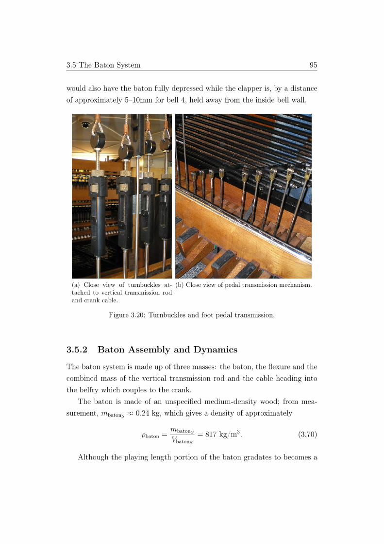
3.5 The Baton System 95
would also have the baton fully depressed while the clapper is, by a distanceof approximately 5–10mm for bell 4, held away from the inside bell wall.
(a) Close view of turnbuckles at-tached to vertical transmission rodand crank cable.
(b) Close view of pedal transmission mechanism.
Figure 3.20: Turnbuckles and foot pedal transmission.
3.5.2 Baton Assembly and Dynamics
The baton system is made up of three masses: the baton, the flexure and thecombined mass of the vertical transmission rod and the cable heading intothe belfry which couples to the crank.
The baton is made of an unspecified medium-density wood; from mea-surement, mbatonS ≈ 0.24 kg, which gives a density of approximately
ρbaton =mbatonS
VbatonS= 817 kg/m3. (3.70)
Although the playing length portion of the baton gradates to becomes a

3.5 The Baton System 96
cylinder, the change in diameter is so slight it is fair to assume the entirebaton length to be in the shape of a rectangular prism. Also, for the restof this section no distinction will be made between natural and sharp keys;the following equations describe both and the coupling to the crank is closeenough to equal because of the ratio l1 : l2.
The flexure has a mass mflexure ≈ 0.05kg, and the rod a mass of mrod ≈0.15kg. The rod is constrained to move vertically by the horizontal woodenbar positioned just below the turnbuckles.
As the baton rotates clockwise the flexure compresses and the rod ispushed against thin felt attached to the inside of this wooden bar; this in-troduces some position-dependent friction which is important to model —particularly in higher bells — and simplifies the baton’s equation of motion:the rod’s centre of mass is always perpendicular to the baton, minus the ba-ton’s slight rotation, and located at distance l6 =
√l22 + (lrod/2)2 from the
baton’s pivot point.The baton system’s centre of mass is
rcom =
[cos θbaton − sin θbaton
sin θbaton cos θbaton
]·
l2/2 ımrod(lrod/2)
mrod +mbaton
(3.71)
where the y component of the actual baton’s centre of mass lies directly inline with the rotation point so does not contribute a weight to ybaton. 6
6Figure 3.15 shows the baton rotation about a circular cut at the non-playing end;this is generally accurate but changes from carillon to carillon. The National Carillon,for instance, rotates by way of a thin leather strap attached to the end of the baton andwrapped around a plastic ‘button’, minimising friction.

3.5 The Baton System 97
So,
τbaton = −g([
1 0]T· rcom
)mbatonAll
= −g cosϕCOMbaton(||rcom||mbatonAll)
ϕCOMbaton = tan−1(ybatonxbaton
)mbatonAll = mbaton +mrod +mflexure (3.72)
and the moment of inertia about the baton pivot, Ibaton, is
Ibaton =1
12mbaton(4l21 + l4) +mflexurel
22 +mrodl
26, (3.73)
with the actual inertia values about the pivot for both sharp and naturalkeys listed in Table 3.3.
3.5.3 Baton System Values
From Eq. (3.60) describing keyfall at the keyface a value for either θbottom orθtop can be determined if the other is known; however, they are quite closeto being equal, and the WCF standards observe that they should be equal,so it is fair to re-write this equation as:
total keyfall↓y =
∫ θmax
−θmax
(l1 − l5) cos θ dθ (3.74)
and solve for θmax using the known baton lengths and keyfalls.
θmax = sin−1total keyfall↓y
2(l1 − l5)(3.75)
The shorter, sharp baton will naturally exhibit a greater rotational displace-ment than the natural baton. The total rotational range for either baton isthen θtotal = 2θmax.
This is an important result for the next section on the kinematics of the

3.6 Baton and Crank Coupling 98
linkage between crank and clapper systems; it is used to determine the totalcrank rotational displacement θcrankmax (in Table 3.2) in the same way as thebaton’s was in the above Eq. (3.75).
Table 3.3: Baton system parameters and calculated values.
Baton System
Parameter Value
rCOMS(27.5 m, 31.65 ◦)
rCOMN(33.2 m, 21.14 ◦)
m3S 0.44 kgm3N 0.52 kgI3S 0.0501 kg· m2
I3N 0.0818 kg· m2
l1S 43 cml1N 56 cml2 l1/2l3 2.5 cml4 2.5 cml5S 13.6 cml5N 20.4 cmmbatonS 0.24 kgmbatonN 0.32 kgmflexure 0.05 kgmrod 0.15 kgtotal keyfall ↓y 4.45 cmθtotalS 8.67 ◦
θtotalN 7.17 ◦
θmax θtotal/2
3.6 Baton and Crank Coupling
As the baton rotates clockwise, a constraint introduced by the flexure and thefelt-lined wooden beam keeps the rigid transmission rod and some portionof the transmission cable — that portion above the flexure and below theceiling — perfectly vertical; also, all rods and cables going into the belfry lie

3.6 Baton and Crank Coupling 99
in the same plane. As seen in Figure 3.21 the portion of cable in the belfry isperfectly vertical only in the rest position; as the crank rotates so does thiscable, although only by a small amount.
In the following discussion, lb = l2 (half the baton length, from Table 3.3)and lc = ||rbaton|| (the full length of the crank rod going to the baton, fromTable 3.2).
lc
lb
θb
θc
ceiling
flexure
(0,0)
(xb, y )b
(a) Baton in rest position.
lc
lb
θb
θc
ceiling
flexure
(0,0)
(xb, y )b
(b) Baton halfway rotated.
lc
lb
θb
θc
ceiling
flexure
(0,0)
(xb, y )b
x
y
z
(c) Baton fully rotated.
Figure 3.21: Range of baton and crank rotation.
The two systems are constrained such that the absolute distance betweenthe base of the flexure and the tip of the crank rod does not exceed the lengthof the cable. Defining the natural length of the cable between the crank and

3.6 Baton and Crank Coupling 100
baton (including the flexure and rigid portion of cable connected to the flex-ure) as L, the absolute location of the crank pivot as (0, 0) and the absolutelocation of the baton pivot (xb, yb), the rotational relationship between thetwo systems can be expressed by the difference vector representing the cableas:
rcable =
[lc cos θc − [xb + lb cos(θb − θbmax)]
lc sin θc − [yb + lb sin(θb − θbmax)]
]
L = ||rcable|| (3.76)
where (xb, yb) and θbmax are different for sharp and natural batons and θbmax
accounts for the difference in initial angle between the baton and crank. Fromthis equation, the length of the vector is always equal to the length of thecable.
The felt-lined wooden beam and the narrow circular cut in the ceilingregulates the interior angle between the cable and the crank rod at the freely-rotating revolute joint; the flexure and the wooden beam has a similar effecton the interior angle between the flexure and baton. Practically, this reducesthe influence of the difference in absolute position along the x-axis betweenthe crank and clapper, ∆x, and allows a very good approximation of therotational relationship to be determined by considering vertical displacementsalone. This approximation also justifies the use of the constant θbmax in thefollowing terms: ∆x is close to 0 at any point in the rotational range so it isappropriate to set it to 0 at a convenient point, namely the rest position.
So, [lc cos θc − [xb + lb cos(θb − θbmax)]
lc sin θc − [yb + lb sin(θb − θbmax)]
]=
[0
L
](3.77)
which, after substituting in boundary conditions θc = 0 when θb = θbmax gives
lc sin(0)− yb − lb sin(0) = L
yb = −L

3.7 Crank and Clapper Kinematics 101
-3.58 -2 2 3.58Θb °
-2
-4
-6
-8.37
Θc °natural baton ® ΘcHΘbL
(a) Natural baton.
-4.34 -2 2 4.34Θb °
-2
-4
-6
-7.76
Θc °
sharp baton ® ΘcHΘbL
(b) Sharp baton.
Figure 3.22: Crank rotation as a function of baton rotation from Eq. (3.78).
and a value for xb that is different for natural and sharp batons but is calcu-lated from the above equation and substitutions simply as
lc cos(0)− xb − lb cos(0) = 0
xb = lc − lb
so xb is negative then positive for natural and sharp batons respectively.These simplifications allow us to fully express θc in terms of θb under the
condition that the cable linking the two systems is taut:
θc = sin−1(lb sin(θb − θbmax)
lc
)(3.78)
This condition of tautness holds most of the time, including all of thetime that the carillonneur is applying force to the baton. However, there aremoments after an impact with the upper or lower wooden beams that the ca-ble slackens and the baton, crank and clapper systems rotate independently.This is accounted for by the virtual spring model developed in next chapter.
3.7 Crank and Clapper Kinematics
Figure 3.23 illustrates the coupling between the clapper and crank mecha-nisms; again, bell 4 is used as a base model for the forthcoming analysis.Vectors describing the length and position of the lever arms for the clapper

3.7 Crank and Clapper Kinematics 102
and crank mechanisms are shown with the cable linking the two, as well asa reference line connecting the two pivot points, or grounds. Note that thelever arm for the clapper system is the vector rcrank, and is offset from thevalue θclapper by +16.97 ◦.7 This value is denoted by θoff for the rest of thissection.
This coupling between the clapper and the crank creates a kinematicallyclosed linkage with one degree-of-freedom where the clapper angle θclapper isdriven by the crank angle θcrank if the player is applying force to the baton,and vice-versa if not. The cable in Figure 3.23 is not drawn as a fixedlength because under certain circumstances it can lose tension and changelength; in the unusual case that it does, the crank and clapper systems rotateindependently until the cable returns to its natural length — this is discussedin the next chapter on dynamics.
However, assuming that the cable linking the crank and clapper is taut,as it is in normal use, the forward kinematics of the linkage can be solvedusing the procedure for determining those of a four-bar mechanism.
Rotating Figure 3.23 clockwise by ψ degrees and re-labelling links andangles, we arrive at the familiar representation of the four-bar linkage inFigure 3.24.
A few more variables are required for the formulation of a closed kinematicloop: ψ maintains an orientational reference to the positive X-axis on this XYplane, and l1 is required as the ‘base’, or fixed link of the four-bar mechanism.The lengths labelled l1 and a in Figure 3.23b were measured directly at bell4 and the angle ψ was determined through the trigonometric relationship
ψ + sin−1(a
l1
)= π.
Referring now to Figure 3.24 one sees that the four-bar mechanisms con-sists of three moving links (input, coupler, and output links) of lengthsl2, l3 and l4 respectively, whose orientations with respect to the horizon-tal are denoted by the angles θ, α and ϕ. From the previous figure, the baselink, l1, is simply the distance between the crank and clapper pivot points;l2 = ||rclapper||, l4 = ||rcrank||, and l3 is the natural length of the cable join-
7See Table 3.1

3.7 Crank and Clapper Kinematics 103
rcrank
crankβ - θ
θclapper
rclapper
cable
≈ 17o
(a) Clapper and crank systems illustrated; including the16.97 ◦ difference between the lever arm rcrank and referenceangle θclapper.
(b) Determination of angle ψ; the lengths l1,a and b were measured on-site.
Figure 3.23: Clapper and crank coupling arrangement (not drawn to scale).
ing the two. The angles θ and ϕ represent the relative displacements of thecrank and clapper angles, respectively while the angles α′ and σ′ represent

3.7 Crank and Clapper Kinematics 104
the angles formed between the cable and the crank and clapper lever arms,respectively.
Figure 3.24: Clapper and crank coupling arrangement as classic four-bar linkage.
3.7.1 Position Analysis
The position analysis of the four-bar mechanism begins with writing theloop-closure equations in the following form:
l2 cos θ + l3 cosα + l4 cosϕ− l1 = 0 (3.79a)
l2 sin θ + l3 sinα− l4 sinϕ = 0. (3.79b)
These equations are re-arranged and squared such that α is eliminated us-ing the identity sin2 α + cos2 α = 1, revealing the well-known Freudensteinequation:
k1 cos θ + k2 cosϕ− k3 − cos(θ + ϕ) = 0 (3.80)
where k1−3 are the Freudenstein parameters, and encapsulate the length ra-tios of the links in the mechanism as
k1 ≡l1l4
k2 ≡l1l2
k3 ≡l21 + l22 − l23 + l24
2l2l4. (3.81)

3.7 Crank and Clapper Kinematics 105
Expanding Eq. (3.80) and collecting the output angle terms, the equationcan be arranged in the general form
−k3 + k1 cos θ + k2 cosϕ− cos θ cosϕ+ sin θ sinϕ = 0
A(θ) cosϕ+B(θ) sinϕ+ C(θ) = 0 (3.82)
where the coefficients A(θ), B(θ) and C(θ) are equal to:
A(θ) = k2 − cos θ
B(θ) = sin θ
C(θ) = −k3 + k1 cos θ. (3.83)
Having arranged Freudenstein’s equation into the general form of Eq.(3.82), we can determine an algebraic solution by means of a transformationof the trigonometric equations into an algebraic equation using the tan-half-angle identities:
tan(ϕ
2
)≡ τ
sinϕ ≡ 2τ
1 + τ 2
cosϕ ≡ 1− τ 2
1 + τ 2. (3.84)
Upon substitution of the above identities into Eq. (3.82), the followingquadratic equation in τ is obtained:
D(θ)τ 2 + E(θ)τ + F (θ) = 0 (3.85)

3.7 Crank and Clapper Kinematics 106
where
D(θ) = C(θ)− A(θ) = −k2 − k3 + (k1 + 1) cos θ
E(θ) = 2B(θ) = 2 sin θ
F (θ) = A(θ) + C(θ) = k2 − k3 + (k1 − 1) cos θ (3.86)
and where the two roots of τ are found using the quadratic solution
τ =−E(θ)±
√E(θ)2 − 4D(θ)F (θ)
2D(θ)(3.87)
with ϕ then found using the identity in Eq. (3.84)
ϕ = 2 tan−1 τ. (3.88)
Plugging the known length values l1−4 (shown in Table 3.4) into Eq. (3.81)and then solving Eqs. (3.86–88) for input angle θ where θcrank = 0, indicatingthat the crank is in rest position8
ϕ(θcrank) = f((β − ψ)− θcrank) = f(θoff − θcrank)
ϕ(θcrank) = f(−8.62 ◦ − 0 ◦) (3.89)
where f(θ) encapsulates the algorithm described over the previous two pages,gives us the two results:
ϕ(0) = 167.36 ◦ and 197.75 ◦ (3.90)
Adding ψ to the two results in order to rotate the four-bar configurationcounter-clockwise and returning it to the natural configuration of the clap-per/crank mechanism, we see these results become 289.93 ◦ and 320.32 ◦, ofwhich the former is clearly the result that does not violate the constraint of
8The crank angle θcrank is subtracted here because the angle is measured clockwise fromthe positive x-axis, unlike the clapper angle which is measured counter-clockwise from thesame axis.

3.7 Crank and Clapper Kinematics 107
the bell wall. This indicates that the set of results for the carillon’s particularconfiguration come from the positive quadratic solution.
bell wall limit
rubber stopper limit
9jHΘL IΘoff - ΘcrankmaxM £ Θ £ Θoff =
-90 -60 -30 30 60 90Θ °
155
165
170
175
j °
(a) Plot of output angle ϕ as input angle θ goes from ±90 ◦.
(b) Illustration of four-bar configurations with θ = ±90 ◦.
Figure 3.25: Plot of output angle as function of input angle.
From the values in Table 3.4, Figure 3.25a plots the positive solution forthe output angle ϕ against the input angle θ = ±90 ◦, with the correspondingset of configurations shown in Figure 3.25b; constraints imposed by the belland rubber stopper are included for reference and are denoted by the shadedarea, with θcrankmax having been determined in the previous section. Theshaded area covers all possible values of ϕ(θ) while θ is within the range of

3.7 Crank and Clapper Kinematics 108
the crank’s rest position and its maximum.This large range of motion is not possible between the crank and clapper
but is plotted to provide a better idea of the relationship. Behaviour withinthe narrow range of legal values is quite linear.
2 4 6 8Θcrank °
271.5
272.0
272.5
Θclapper °
Θclapper HΘoff - ΘcrankL
(a) θclapper as a function of θcrank withinlegal range, and after orientation from Eq.(3.91).
2 4 6 8Θcrank °
96.45
96.50
96.55
Α °
Α HΘcrank, ΘclapperL
(b) α as a function of θcrank and θclapper.
2 4 6 8Θcrank °
68
70
72
74
Α' °
Α' HΘcrank, ΘclapperL
(c) Angle formed between cable and cranklever arm.
2 4 6 8Θcrank °
69.5
70.0
70.5
Σ' °
Σ' HΘcrank, ΘclapperL
(d) Angle formed between cable and clap-per lever arm.
Figure 3.26: Plot of output angle as function of input angle in legal range of motion.
Focusing on the shaded area from Figure 3.25a the crank input and clap-per output values are adjusted by first adding +ψ, re-orienting the mecha-nism to the real crank/clapper linkage, and then subtracting 16.97 ◦ in orderto get the angle θclapper in place of the angle for the lever arm described byrclapper:
θclapper(ϕ) = ϕ(θcrank) + ψ − θoff. (3.91)
This is then plotted to reveal the actual range of motion in Figure 3.26a,which is seen to be very small. For completeness, the angle α describing

3.7 Crank and Clapper Kinematics 109
the orientation of the cable l3 and the horizontal is also plotted, as are theangles α′ formed between the cable and the crank’s lever arm, and σ′, formedbetween the cable and the clapper’s lever arm.
These three angles can be calculated once θ and ϕ have been found; αis determined simply by rearranging the original loop closure equations Eqs.(3.79a–b) and solving for α while plugging in θ and ϕ(θ). The angles α′
and σ′ are determined using results for the other angles and applying simpletrigonometry.
While the boundary values for θclapper are very close to 270 ◦ and wouldseem to afford little opportunity for torque due to gravity acting on theclapper’s mass, recall from the earlier §3.3 that, in the case of bell 4, theclapper’s centre of mass is offset from this angle by approximately +11 ◦.
3.7.2 Length Analysis and Other Bells
To simplify future dynamic calculations, results from the algebraic formula-tion presented in the preceding few pages are fitted to a linear model, withparameters estimated from physical measurements. Such a model decreasesthe level of expertise required to model a novel kinematic arrangement in aforeign carillon.
This approach also mitigates the influence of a necessary feature of caril-lon design: that each unique geometric variable does not change continuouslyacross the entirety instrument. For instance, the value b labelled in Figure3.23b denoting the horizontal distance between the crank pivot point and theclapper pivot point only changes in groups of seven or so bells; this is thenumber of bells that are typically mounted in plane on the same aluminiumbeam, thereby fixing their absolute position, and crank shafts necessarily liein a uniform plane because of their coupling to the clavier below.
Linear Fitting, Bell 4
The plot in Figure 3.26a for θclapper as a function of θcrank shows that therelationship is quite linear within the narrow range of legal values.

3.7 Crank and Clapper Kinematics 110
Figure 3.27: Two rows of mid-range bells. The cranks lie in the same horizontalplane but are vertically staggered whilst each row of bells is fixed both horizontallyand vertically.
A simple linear model of the form
θclapper = β1θcrank + β2 (3.92)
is fitted to the motion calculated by the more accurate kinematic solution.The residuals as a percentage of the total clapper rotation are shown inFigure 3.28. The linearisation clearly misses the trigonometric nature of therelationship, but the magnitude of error is quite small.
The linear least-squares fit for bell 4 returns β1 = 0.192 and β2 = 271.15.The former value relates the linear change in clapper motion as the crankrotates, and is approximately equal to the ratio of the crank length to theclapper length β1 ≈ l2/l4. The latter value approximates the clapper startangle.

3.7 Crank and Clapper Kinematics 111
1 2 3 4 5 6 7 8Θcrank °
-0.4
-0.2
0.2
% error °Bell 4 linear fit residuals
Figure 3.28: Residuals for linear fit of bell 4 kinematics
Bells 28 and 55
Length data was also measured for bells 28 and 55. Figure 3.29 shows theclapper output angles as a function of crank motion. The relationship re-mains quite linear despite an increase in the range of clapper rotation from1.59 ◦ for bell 4 to 3.82 ◦ and 10.05 ◦ for bells 28 and 55 respectively. The fitresiduals match the shape of those for bell 4, but increase in magnitude to0.5% and 1.2% of the range for bell 28 and 55, respectively.
2 4 6Θcrank °
281
282
283
284
Θclapper °
bell 28 Θclapper HΘcrankL
(a) Bell 28 clapper angle versus crank angle.2 4 6 8
Θcrank °
284
286
288
290
292
Θclapper °
bell 55 Θclapper HΘcrankL
(b) Bell 55 clapper angle versus crank angle.
Figure 3.29: Bells 28 & 55 clapper angles versus crank.
The linear fits for these two bells follows the same pattern as for bell 4.The proportional change for both is approximately the ratio between crankand clapper lengths, and the constant is the clapper start angle.

3.7 Crank and Clapper Kinematics 112
ò
ò
ò
0.4 0.6 0.8 1.0 1.2 1.4l4
274
276
278
280
282
284Θmin °
Clapper start angle fitted to clapper length
(a) θmin = −10l4 + 285.4
ò
ò
ò
0.4 0.6 0.8 1.0 1.2 1.4l4
0.6
0.8
1.0
1.2
1.4
1.6
l1Length l1 fitted to clapper length
(b) l1 = l4 + 0.16
Figure 3.30: Clapper length as a predictor of clapper/crank kinematics.
Estimating Length and Clapper Angle Parameters
In Chapter 6, it is shown that the clapper length l4 can be estimated quitewell across the range of the instrument, based on a correlation with elementsof carillon bell design that are somewhat standardised across instruments.This makes clapper length a useful value upon which to base estimates ofother physical values.
An estimate for the clapper start angle (the constant β2 in Eq. (3.92))can be made from the clapper length l4. The plot in Figure 3.30a shows thelinear fit relating clapper lengths to clapper start angles calculated from thekinematic equations and measured lengths a and b.
This linear fit has a physical basis related to the torque due to gravityacting on the clapper mass and clapper angle. Clapper pivots for the lowsbells are fixed off-centre and closer to the bell wall in order to limit the torquedue to gravity acting on the massive clapper masses. As clappers becomelighter they tend to be positioned closer to their bell’s centre, and require alarger start angle in order to reach the bell wall.
The absolute length l1 between the clapper pivot and the crank pivotis another important value to estimate across the range of the instrument;this length is the hypotenuse of the triangle formed by the horizontal andvertical distance between the two pivot points. The plot in Figure 3.30bshows that this value is proportional to clapper length l4. Depending onbell geometry, this length can be decomposed into arbitrary horizontal and

3.7 Crank and Clapper Kinematics 113
vertical components.Table 3.4 contains the measured and calculated data for bells 4, 28 and
55.
Table 3.4: Crank to Clapper Linkage as Four-bar Mechanism Parameters for Bells4, 28 and 55.
Crank to Clapper Linkage
Bell Parameter Value
Bell 4 (B2) θclappermax272.76 ◦
θclappermin271.15 ◦
ψ 122.39 ◦
θoff 17 ◦
a 1.34 mb 0.85 ml1 1.59 ml2 0.27 ml3 0.39 ml4 1.41 m
Bell 28 (B4) θclappermax284.89 ◦
θclappermin280.79 ◦
ψ 131.01 ◦
θoff 10 ◦
a 0.46 mb 0.40 ml1 0.61 ml2 0.26 ml3 0.275 ml4 0.505 m
Bell 55 (D7) θclappermax292.95 ◦
θclappermin282.91 ◦
ψ 142 ◦
θoff 5 ◦
a 0.25 mb 0.32 ml1 0.41 ml2 0.26 ml3 0.24 ml4 0.21 m
3.8 Summary 114
3.8 Summary
This chapter has presented physical data collected from the National Car-illon. This data was used to develop a rigid body model of the clapper forbell 4, in a manner that can be applied to any of the other clappers. Thethorough understanding of the physical characteristics of this particular clap-per underpins later work in this thesis, namely by providing a known andaccurate base upon which to build physical models for other clappers thathave not been measured.
The kinematics of the linkage between the clapper and crank systemswere solved algebraically. The motions were then shown to be sufficientlyclose to linear that they can be modelled as simple linear equations; suchequations were found through linear least-squares estimation for bells 4, 28and 55. A further set of linear relationships was identified relating bothclapper start angle and absolute distance separating crank and clapper pivotto clapper length; clapper length itself is a key parameter linking changingclapper geometry to variation in bell size across the instrument. A scalinglaw for clapper lengths based on carillon bell design is developed in Chapter6.

Chapter 4
Haptic Model
4.1 Stages of Rotational Motion
Armed with the physical and geometric data of the previous chapter, wedevelop two dynamic models for evaluation against the behaviour of bell 4at the National Carillon: one is kinematically constrained and the other isdynamically constrained.
The kinematically constrained model reduces the entire carillon mecha-nism to a single degree-of-freedom, single body problem in which the threerotational coordinates are linearly related but only one is integrated duringcomputation. The dynamically constrained model integrates the three coor-dinates separately but uses unilateral constraints, namely virtual springs, toexchange forces between the systems.
4.1.1 Static Equilibrium at Rest
When the system is at rest, the baton at its minimum displacement and heldagainst the felt-lined wooden upper beam. At the same time, the crank is alsoat zero displacement with its straight rod lying parallel to the positive x-axis,and the clapper is also at its minimum displacement — i.e. the maximumdistance from the inside of the bell wall.
The baton system is prevented from rotating under the downward forceof gravity and its mass m3 by upward force exerted by tension in the cable B

4.1 Stages of Rotational Motion 116
l1
l2C
l2B
l3
θ3
θ1
x
z
y
θ2
B
C
(a) Length and angles for reference againstvalues determined in the previous chapterand physical constraints for the baton andclapper systems.
m1
m2
m3
+Tc
+Tc
‐TB
+TB
lc1
lc2
lc3(b) Statics of the carillon mechanism, in-cluding tension forces from linkage cables.
Figure 4.1: Mechanical representation of bell 4 dynamics.
linking it to the crank, +TB; the system is kept at equilibrium by the staticfriction between the baton and adjacent metal bars and the reaction forceFfelt between the top of the baton and the upper wooden beam.
Depending on which bell is under consideration, there are two ways theclapper system is prevented from rotating further away from the bell underthe force of gravity and its mass m1. In high bells the tension TC in the cableC alone prevents the clapper from moving back; in lower bells with heavierclappers a rubber damper also prevents the clapper from continuing awayfrom the bell.
Ideally, the rubber damper and the upper wooden beam share the clap-per’s load, that is to say the system is calibrated such that the clapper returnsto its minimum displacement at the same time the baton does. This rela-tionship is regulated by a turnbuckle in B that adjusts its length: shorteningB increases the baton’s natural starting angle and brings it closer to, or infirmer contact with, the upper beam.
As well as damping the contact between the baton and the upper wooden

4.1 Stages of Rotational Motion 117
beam, the layer of felt between the upper beam and the baton acts as acompression spring. For the baton system to remain at static equilibriumthe reaction force from this felt, the tension in the cable and the torque dueto baton mass and gravity must cancel each other out.
That is:
TBl3 − τF (θ3)− τ3(θ3, θ3) = θ3I3
= 0 (4.1)
where τ3(θ3, θ3) is the torque resulting from baton mass components andgravity and includes friction, TBl3 is the torque from the tension in cable Band τF (θ3) the reaction torque from the felt.
At this stage, the crank is also motionless, with TC and TC cancellingeach other out1
τ2(θ2) + TC l2C − TBl2B = θ2I2
= 0 (4.2)
When the baton is not in contact with the felt then TBl3 is equal to thetorque due to gravity acting on m3, and clapper load is borne almost entirelyby its rubber damper.
If the baton is in contact with the felt and B is then shortened, therestoration force from the felt increases so that further shortening begins topull the clapper toward the bell and diminishes the influence of the rubberdamper. With this, the tension TB increases linearly with the reaction forceFfelt.
Good carillon design aims to have the clapper load balanced fairly equallybetween the upper beam on the clavier and the rubber damper in the bell,smoothing the increase in force-feedback as a carillonneur beings their stroke.
1Ignoring for the moment the minor static role of the crank’s centre of mass.
4.1 Stages of Rotational Motion 118
4.1.2 Player-applied Downward Force
As the player applies a downward force and the baton begins to rotate down-ward, it is no longer in contact with the upper beam felt and the clappersystem is no longer in contact with the rubber damper. The system’s motionis described by the dynamics of the respective subsystems, the cable linkagesand the magnitude of the downward force applied by the player.
4.1.3 Let-off and Clapper Free-flight to Impact
As the baton approaches the lower wooden beam the clapper approachesthe inside of the bell wall. If the length of cable B is properly adjusted thebaton will reach its absolute maximum displacement (including some smallcompression of the felt separating the bottom of the baton from the woodenlower beam, similar to the upper beam) before the clapper impacts with thebell. Ideally, the clapper will be approximately 3–5 mm from the bell wallat the point where the baton can not be depressed any further.
Adopting the terminology of the literature for the modelling of the dy-namics of the grand piano [52] [69] [93] the term ‘let-off’ is used to describethe phase that begins when the baton first comes into contact with the felt-lined lower beam and ends when the baton can longer compress the felt anymore. If the baton’s velocity is high enough cable B begins to lose tensionduring this phase as the clapper continues to move toward the bell while thebaton is unable to rotate any further; during this phase the force-feedbackexperienced by the player is increasingly constituted simply of the reactionforce from the felt until the ‘free-flight’ phase where the baton is maximallydepressed and has no further influence on the clapper’s motion.
As the clapper strikes the bell there is a transfer of energy that resultsin the bell sounding and the clapper being pushed away from the bell; if thelength of B is correctly configured the carillonneur should not be able tohold the clapper against the bell. Theoretical and empirical work analysingthe impact between the clapper and bell by Fletcher [42] and refined in thischapter shows that the clapper remains in contact with the bell for about0.6–1.5 msec. The clapper remains in contact with the bell until transverse

4.1 Stages of Rotational Motion 119
pulses propagated in both directions around the sound bow of the bell atimpact complete their circuit and dislodge the clapper from the impact site.
Linkage Modelling
The Newton-Euler model takes advantage of a possible simplification regard-ing the linkages between the baton, crank and clapper systems. As shownshown in §3.6 and §3.7 on baton/crank kinematics and crank/clapper kine-matics, the relationship between each of the systems’ displacements can beapproximated linearly, leading to an assumption of uniform velocity.
This means only one coordinate is required to describe the system; theangular acceleration and velocity of any two systems are linearly dependanton that of one other in which case only the latter needs to be calculated overtime. This has the advantage of minimising the computations required tosolve the system in real-time and also keeping the conceptualisation of thesystem reasonably simple. The approach requires that we solve for constraintforces introduced by the cables. This linearisation also opens the door toleast-squares fitting techniques.
One disadvantage of this approach is that it depends on modelling thelinkage cables as ideal and constantly-present force interactions. In reality,the cables behave more like extremely stiff extension springs that only gener-ate a restoration force when stretched to be greater than their natural length.It is not possible to pull the clapper away from the bell wall by pulling thebaton up, for instance; in response to such a gesture the cable linking thebaton to the crank loses tension and the baton is mechanically uncoupledfrom the rest of the system until tension is restored.
Another situation in which the cable linking the baton and crank losestension is in the brief ‘let-off’ phase where the clapper is in free flight towardthe inside of the bell wall. During this phase the baton is at its maximumdisplacement while the crank and clapper continue rotating.
This cable is also responsible for perceptually significant mechanical back-lash on many bells, particularly at the lower end of the carillon range. Asthe baton mass is so slight compared to that of the low clapper the cable

4.1 Stages of Rotational Motion 120
is not fully taut prior to the application of player force. A further dynamicconsequence arising from the linkage cables is a type of ‘stick-slip’ baton mo-tion for higher bells as the baton returns to the rest position in free motion.In this case, the return forces in the tower for higher bells — including theclapper mass and any return springs — are only just large enough to pullthe baton back. Friction in the baton system is introduced between the feltlinings and the clavier’s structure, and at the plastic/leather pivot: the com-bination of a cable which is not particularly taut and this friction may retardand occasionally briefly halt the baton’s motion.
Friction Modelling
The study of friction modelling is increasingly sophisticated as friction com-pensation is a particularly fruitful area for improving the performance ofsystems for controlling actuators [96]. In studies examining haptic percep-tion of friction, and friction models for general haptic rendering, the relativelysimple Karnopp friction model has been demonstrated to be effective [105]. Itis also suitable for linear least-squares fitting techniques, with Richard [105],Swindells and Maclean [117], and Colton and Hollerbach [29] each using thismodel in haptic applications.
The Karnopp friction model is a function of velocity and the sum of non-frictional torque applied to the system, and includes Coloumb (dynamic),static and viscous friction while allowing for asymmetric friction values forpositive and negative forces:
τfric(θ, τa) =
Cn sgn(θ) + bnθ, θ < −∆ω
max(Dn, τa), −∆ω < θ < 0
min(Dp, τa), 0 < θ < ∆ω
Cp sgn(θ) + bpθ, θ > ∆ω
(4.3)
The Karnopp model produces stick-slip friction by assigning a velocityregion −∆ω < θ < ∆ω over which a force is returned equal to the sum ofnon-frictional forces applied to the system — allowing no change in velocity

4.2 Zero Relative Velocity 121
— until the applied torque exceeds a break-away torque specified by Dn orDp. Outside of this region, friction is specified by the sum of dynamic andviscous friction, weighted by C and b respectively.
The physically-motivated structure of this model also makes it suitable fornon-expert parameter estimation, as rough estimates of static and dynamicfriction can be made by taking force measurements at the baton.
4.2 Zero Relative Velocity
In this section, the classical kinematically-constrained Euler-Lagrange equa-tions are used to reduce the carillon mechanism model to a single-DOF, singlebody problem.
The three rotational systems are linked in series by two thin-wound steelcables; these are modelled as thin and inextensible rods and they are cou-pled to the respective systems by frictionless revolute joints. Their mass isincorporated into the baton and crank masses.
The first rod links the tip of the clapper system at a distance l1 from itspivot to the tip of the clapper-fly in the crank system at a distance l2C fromthe crank’s pivot; the second rod links the tip of the other crank rod at adistance l2B from the pivot to the baton’s flexure at a distance l3 from thebaton’s pivot.
This method assumes a constant angle formed between cables and themoment arms of the respective rotational systems; the angles themselvesare selected from the analysis in §3.6 and §3.7, and are refined against thebehaviour of the energy model presented in the next section.
To recast the problem as a kinematically constrained system, the pointsmarking the revolute joints are required to maintain a relative velocity ofzero. Each of these linkage points are constrained to move at the same rateas each other so the respective rotational velocities and accelerations areconstrained.

4.2 Zero Relative Velocity 122
4.2.1 Classical Formulation
The Euler-Lagrange dynamic equations
Mθ = τ + ATλ (4.4)
describes a system of n rotational coordinates θ which have inertia M andare constrained by m holonomic and/or nonholonomic constraints A whichsatisfies
Aθ = 0 (4.5)
and λ is a m × 1 vector of constraint force magnitudes (Lagrangian multi-pliers) and forces not due to constraints or inertial properties like springs,dampers or gravity are encompassed in τ .
The inertia matrix is made up of the moments of inertia for the respectiverotational systems
M =
I1 0 0
0 I2 0
0 0 I3
(4.6)
The external force matrix is expressed as
τ =
(m1lc1g cos(θ1 + ϕ1)
+ k(θ1o − θ1)
)0 0
0 m2lc2g cos(θ2 + ϕ2) 0
0 0
(m3lc3g cos(θ3 + ϕ3)
+ τfric + τu
)
(4.7)where k is the clapper spring constant, θ1o is the spring offset, and τfric issystem-wide friction, applied here at the baton. User-applied torque at thebaton is represented as τu. Because we plan to reduce the system to a single-body problem, forces due to the spring and friction could have been includedin any of the three torque expressions.
The three rotational coordinates are kinematically constrained to zero

4.2 Zero Relative Velocity 123
relative velocity by the following holonomic relations
θ1l1 + θ2l2C = 0 (4.8a)
θ3l3 − θ2l2B = 0 (4.8b)
and, by substitution
θ1l1 + θ3l3l2B
l2C = 0 (4.8c)
where the signs change to indicate that the clapper rotates in the oppositedirection to the crank and baton during motion.
These expressions can be integrated to express position constraints asfunctions of baton rotation:
θ1(θ3) = (θ3 − θ3min)l3l2B
+ θ1min
θ2(θ3) = (θ3 − θ3min)−l2C l3/l2B
l1+ θ2min (4.9)
Taking the first two relations in Eqs. (4.8a–c) the constraint matrix isdesigned
A =
[l1 l2c 0
0 −l2b l3
](4.10)
in order to meet the condition in Eq. (4.5).The Lagrangian multipliers represent the tension forces in the cables TC
and TB over the carillon’s limited range of motion; with the notation fromFigure 4.1
λ =
[TC
TB
](4.11)
then,
ATλ =
TC l1
TC l2C − TBl2BTBl3
. (4.12)

4.2 Zero Relative Velocity 124
4.2.2 Simplifying Reaction Forces
Plugging the matrices from the previous subsection into Eq. (4.4) yields thefollowing system of equations:
I1θ1 = τ1(θ1) + TC l1
I2θ2 = τ2(θ2) + TC l2C − TBl2BI3θ3 = τ3(θ3, θ3, τu) + TBl3
(4.13)
This system can be expressed entirely in terms of baton acceleration θ3by solving the above for TB by first solving for and eliminating TC and thenusing the acceleration relations to derive a linear function of the weightedsum of the three torque functions:
TB(τ1, τ2, τ3) =3∑i=1
wiτi (4.14)
with
w1 = −I3l1l2B l2Cwall
w2 =I3l2B l
21
wall
w3 = −l3(I2l
21 + I1l
22C
)
wall
wall = I3l21l
22B
+ l23(I2l21 + I1l
22C
) (4.15)
Plugging this expression into the bottom row of Eq. (4.13) and using therelations in Eqs. (4.8a–c) to update values for θ1 and θ2 provides a simplecomputational model of carillon motion in response to player-applied force.
4.2.3 Linearisation
A further simplification prepares the model for linear least-squares fittingin the case that length or inertia parameters are not known. Each of the
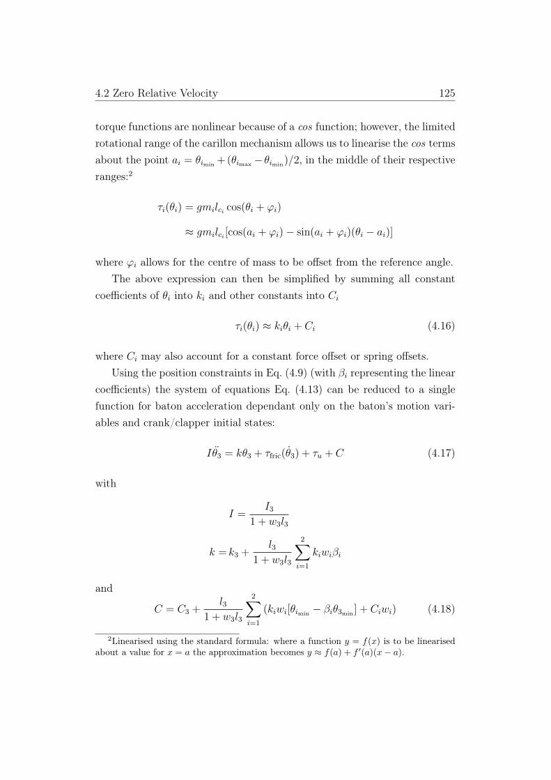
4.2 Zero Relative Velocity 125
torque functions are nonlinear because of a cos function; however, the limitedrotational range of the carillon mechanism allows us to linearise the cos termsabout the point ai = θimin + (θimax− θimin)/2, in the middle of their respectiveranges:2
τi(θi) = gmilci cos(θi + ϕi)
≈ gmilci [cos(ai + ϕi)− sin(ai + ϕi)(θi − ai)]
where ϕi allows for the centre of mass to be offset from the reference angle.The above expression can then be simplified by summing all constant
coefficients of θi into ki and other constants into Ci
τi(θi) ≈ kiθi + Ci (4.16)
where Ci may also account for a constant force offset or spring offsets.Using the position constraints in Eq. (4.9) (with βi representing the linear
coefficients) the system of equations Eq. (4.13) can be reduced to a singlefunction for baton acceleration dependant only on the baton’s motion vari-ables and crank/clapper initial states:
Iθ3 = kθ3 + τfric(θ3) + τu + C (4.17)
with
I =I3
1 + w3l3
k = k3 +l3
1 + w3l3
2∑i=1
kiwiβi
and
C = C3 +l3
1 + w3l3
2∑i=1
(kiwi[θimin − βiθ3min ] + Ciwi) (4.18)
2Linearised using the standard formula: where a function y = f(x) is to be linearisedabout a value for x = a the approximation becomes y ≈ f(a) + f ′(a)(x− a).
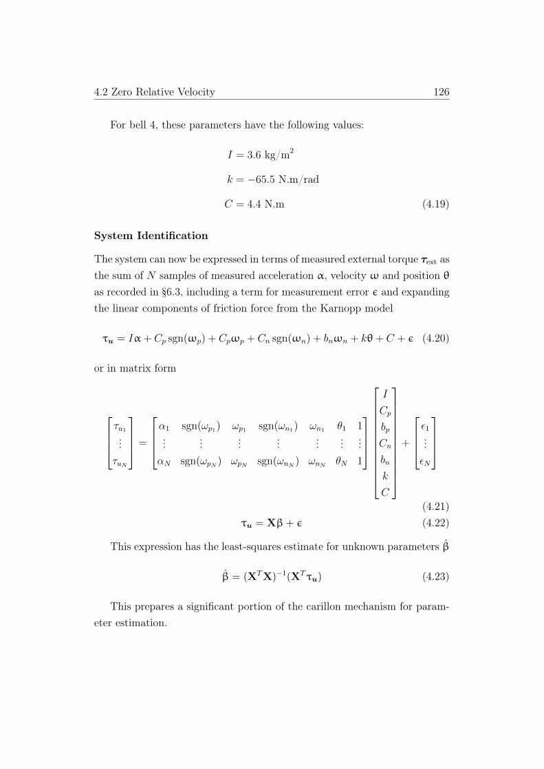
4.2 Zero Relative Velocity 126
For bell 4, these parameters have the following values:
I = 3.6 kg/m2
k = −65.5 N.m/rad
C = 4.4 N.m (4.19)
System Identification
The system can now be expressed in terms of measured external torque τext asthe sum of N samples of measured acceleration α, velocity ω and position θas recorded in §6.3, including a term for measurement error ε and expandingthe linear components of friction force from the Karnopp model
τu = Iα+ Cp sgn(ωp) + Cpωp + Cn sgn(ωn) + bnωn + kθ+ C + ε (4.20)
or in matrix form
τu1...τuN
=
α1 sgn(ωp1) ωp1 sgn(ωn1) ωn1 θ1 1...
......
......
......
αN sgn(ωpN ) ωpN sgn(ωnN) ωnN
θN 1
I
Cp
bp
Cn
bn
k
C
+
ε1...εN
(4.21)τu = Xβ+ ε (4.22)
This expression has the least-squares estimate for unknown parameters β
β = (XTX)−1(XTτu) (4.23)
This prepares a significant portion of the carillon mechanism for param-eter estimation.

4.3 Dynamic Constraints 127
4.3 Dynamic Constraints
An alternative method for formulating equations of motion where severalcoordinates are kinematically constrained is the Lagrangian method of vir-tual work. By considering the respective systems in terms of their kineticand potential energies and carefully observing the nature of their interactionconstraints one is able to formulate equations of motion without explicitlysolving the force interactions between those systems.
The Lagrangian is defined as:
L =n∑i=1
(Ti − Vi) (4.24)
where Ti and Vi are the kinetic and potential energy equations for the respec-tive coordinates, qi. An equation of motion for a conservative system withno external forces is then formulated by
d
dt
(∂Ldqi
)−(∂Ldqi
)= 0. (4.25)
If external and dissipative forces are present in the system they are easilyincluded in the above equation like so:
d
dt
(∂Ldqi
)−(∂Ldqi
)=
n∑i=1
Fqi (4.26)
where Fqi is an external force acting on the coordinate qi. The Karnoppfriction model and impact forces are included here.
Using the uniform acceleration model described in the previous sectionas an example, we would reduce the three coordinates {θ}13 to one, say crankrotation, upon which the other two are dependant. By defining θ1 and θ3 asfunctions of θ2 then expressing the respective potential and kinetic energiesfor Eqs. (4.24–25) we develop an equation of motion without regard for cabletension forces.
However, this only accurately models the entire mechanism during thedownward player-applied force stage. During the let-off and clapper free-

4.3 Dynamic Constraints 128
flight to impact stages the systems rotate independently. The encapsulatingcharacteristic of any stage where the three systems do not rotate uniformlyis that either one of the cables are not taut; the geometric interpretation ofthis is that the distance between two coupling points is less than the naturallength of the cable.
Computing the rotations of the respective systems independently at alltimes also allows us to explore the energy transfers between carillon com-ponents in less common circumstances; for instance, where a loose cable Callows the clapper to move away from the bell under its gravitational poten-tial alone while the carillonneur holds the baton still, the clapper will transfermore kinetic energy to the carillonneur upon cable C regaining tension thanif the player were mechanically coupled to the clapper the entire time.
4.3.1 The Cable-as-Spring and Virtual Springs
k1
k2
r1
Cr2
rc1
rc2
Br2
rc3 r3≈
x
z
y
θ1
φ1
φ2
β
θ2
θ3
(x , y )1 1
(0, 0)
(x , y )3 3
Figure 4.2: Carillon mechanisms coupled with virtual springs.
A simple way of conceptualising the cables is to consider them as very

4.3 Dynamic Constraints 129
stiff springs that only produce a reaction force when stretched; when they areless than their natural length they effectively contribute nothing to the dy-namics of the mechanism and can be removed from the model. Wang et al.’s[127] virtual spring solution to forward and inverse dynamics problems withkinematically constrained mechanisms is the basis for the following work.
Their method is adapted to suit the unilateral nature of the cable-as-spring by allowing the spring to exert force in only one direction, and onlywhen the difference between the absolute position of two coupling points isgreater than the cable’s natural length.
The position vectors can be defined as functions of their respective angles:
r1 = pO1 + Q(θ1) ·
[l1
0
]
r2B = pO + Q(θ2) ·
[l2B0
]
r2C = pO + Q(θ2 + β) ·
[l2C0
]
r3 = pO3 + Q(θ3 + θ3max) ·
[l3
0
](4.27)
where Q is a standard rotation matrix
Q(θ) =
[cos θ − sin θ
sin θ cos θ
]
and the origin position vectors pO = [0 0]T , pO1 = [x1 y1]T and pO3 =
[x3 y3]T are determined from relationships presented in the previous chapter
— their values for bell 4 are listed in Table 4.1.The centres of mass of the respective bodies are similarly defined with
4.3 Dynamic Constraints 130
respect to the offsets ϕi from the body position vectors
rc1 = pO1 + Q(θ1 + ϕ1) ·
[lc1
0
]
rc2 = pO + Q(θ2 + ϕ2) ·
[lc2
0
]
rc3 = pO3 + Q(θ3 + ϕ3) ·
[lc3
0
]. (4.28)
The kinetic energies for the three moving systems can now be written as
T1 =1
2I1θ
21
T2 =1
2I2θ
22
T3 =1
2I3θ
23 (4.29)
where Ii are the moments of inertia for the three systems about their respec-tive pivot points, as calculated in the previous chapter, not about the theirrespective centres of mass as is typically done.
The potential energies, then, are
V1 = m1g(j · rc1) = m1g[y1 + lc1 sin(θ1 + ϕ1)]
V2 = m2g(j · rc2) = m2g lc2 sin(θ2 + ϕ2)
V3 = m3g(j · rc3) = m3g[y3 + lc3 sin(θ3 + ϕ3)] (4.30)
where j = [0 1] is the unit vector along the y axis — the direction of thegravity field.
From [127], the elastic potential of the energy stored in a virtual springis expressed as
Vs =1
2k ||∆||2 (4.31)
where ∆ is the displacement vector of a virtual spring. This vector becomes,

4.3 Dynamic Constraints 131
for cable C and B respectively,
∆1 =
[∆xC
∆yC
]= r1 − r2C
∆2 =
[∆xB
∆yB
]= r2B − r3. (4.32)
Table 4.1: Constants for Simulation of Bell 4.
Parameter Value
m1 61.38 kgm2 1.19 kgm3 0.52 kgI1 69.25 kg·m2
I2 0.063 kg·m2
I3 0.082 kg·m2
l1 1.41 ml2C 0.27 ml2B 0.24 ml3 0.28 mlc1 1.022 mlc2 4.7 cmlc3 33.2 cmls 1.34 mϕ1 −6.19 ◦
ϕ2 68.78 ◦
ϕ3 21.14 ◦
(x1, y1) (-0.85, 1.34) m(x2, y2) (-0.04, -5) mk1, k2 106 N/mkS -322 N/radc -2.2 N/rad/secθS0 301.96 ◦
{θ1, θ2, θ3}min {288.12 ◦, 0 ◦, 3.58 ◦}{θ1, θ2, θ3}max {289.73 ◦, −8.37 ◦, −3.58 ◦}L1 ||r2C (θ2max)− r1(θ1max)|| ≈ 0.39 mL2 ||r2B(θ2max)− r3(θ3max)|| ≈ 5 m

4.3 Dynamic Constraints 132
In order to condition the springs to exert force only in reaction to expan-sion a max function is applied to Eq. (4.31):
Vsi =1
2ki [max(||∆i||, Li)− Li)]2 (4.33)
such that when the difference vector has a length less than the cable’s naturallength Li the squared term is equal to 0, and, hence, the cable vanishes fromthe model.3
Finally, include the potential energy from the forward spring discussed in§3.3.4 which is connected to the tip of the clapper at a distance ls from thepivot. From Eq. (3.48) on page 75 in the section where θS0 is defined, andusing constants defined in Table 3.1, the equation for this spring’s potentialenergy is appended to the existing definition of V1:
V1 = V1 −1
2ls kS (θS0 − θ1)2.
Between the equations just developed, and a set of initial values for {θ}13,a set of equations of motion can be derived from the Lagrangian. The finalconsideration to complete the model is the impact forces to be encapsulatedin the Fqi term.
4.3.2 Comparison of the Two Models
Prior to considering impact constraints, however, the two models are checkedagainst each other. Two of the scenarios in Chapter 6 are simulated: freebaton motion after being released from the bottom of its stroke, and motionwith a mass attached to the baton tip after being released from the top ofits stroke.
The two models are computed using the same physical parameters, takenfrom Table 4.1; Figure 4.3 shows the position error between models to be verylow for both of these scenarios. This result confirms that the linearisationof the kinematically constrained model has retained desirable properties like
3Table 4.1 gives expressions then approximate values for Li; during simulation, numer-ical precision is maintained by using the expression rather than the approximation.

4.4 Mechanical Impacts: Clapper/Bell and Baton/Felt 133
0.05 0.10 0.15 0.20 0.25 0.30 0.35t HsecL
-3
-2
-1
1
2
3
Θ3HtL °Release from bottom
(a) Released from bottom.
0.05 0.10 0.15 0.20 0.25 0.30 0.35t HsecL
-3
-2
-1
1
2
3
Θ3HtL °Release from top with 2.3 kg mass
(b) Release from bottom.
0.05 0.10 0.15 0.20 0.25 0.30 0.35t HsecL
-0.06
-0.04
-0.02
0.02
0.04
0.06
D Θ3HtL °Difference between the two models
From top
From botton
(c) Difference in position of two models.
Figure 4.3: Comparison of the behaviour of the two constraint models.
response to force applied at the baton and the torque due to masses andgravity in the crank and clapper systems.
4.4 Mechanical Impacts: Clapper/Bell and Ba-
ton/Felt
The role of impacts in the carillon system is the transferral of energy froma moving system to a dissipative system. The upper and lower limits ofbaton rotation are enforced by felt-lined wooden beams. The upper limitof clapper rotation is the inside of the bell wall, and the lower limit is therubber damper. The four impact sites are grouped in complementary pairs:clapper/bell impact with baton/lower-beam impact; and, clapper/damperimpact and baton/upper-beam impact. The dynamic model cannot be vali-dated until these impacts are also modelled, as they account for much of the

4.4 Mechanical Impacts: Clapper/Bell and Baton/Felt 134
baton’s motion.Each of the impacts can be modelled as first-order differential systems
that are displaced by a spring-like force during impact; in the case of the bellwall this displacement is the flexural waves that travel around the bell thatcause it to sound, and in the case of the rubber damper the displacement is atemporary plastic deformation. While there are several techniques for mod-elling any of these impacts, it is key to choose those which exhibit hysteresis,or a net loss of energy during impact.
The bell/clapper impact model presented by Fletcher et al. [42] is onesuch model. In the following section some numerical elements of their modelare corrected, and the model is then applied to the baton/damper impact.
4.4.1 Re-calibrated Impact Theory for Clapper/Bell
Impact
The analysis in Fletcher et al. leads to three claims regarding the clapper/bellimpact:
1. An extended impact theory for the collision between clapper and bellthat accounts for a pre-existing ‘impact flat’ on the clapper;
2. Contact times predicted by the extended impact theory are in disagree-ment with contact times empirically observed; and
3. That a wave propagated around the bell at a velocity determined bythe frequency spectrum of the force curve explains this discrepancy.
The extended impact theory uses Hertzian contact law (presented in Gold-smith [55]) as a starting point; this law is also used as a check against re-sults from the extended theory when simulating a Hertzian scenario, namelya spherical body with no impact flat impacting a massive plate of infiniteimpedance. However, whilst the equations and results in Fletcher et al. areinternally consistent and reproducible, they are not in agreement with anindependent evaluation of the Hertzian predictions. Specifically, there are
4.4 Mechanical Impacts: Clapper/Bell and Baton/Felt 135
two values that do not match the results presented in the paper: the totalcontact time and the maximum force (a function of maximum approach αm).
The reproduction of the results from Fletcher et al. in Figure 2.3 (Liter-ature Review, page 47) shows that their model predicts τ ≈ 0.28 msec, andFmax ≈ 70 kN for the Hertzian scenario with no prior impact flat (d0 = 0).
In the following work, the Hertzian equations based on Goldsmith’s pre-sentation [55] are evaluated in order to highlight the discrepancy with theresults in Fletcher et al.; the equations are re-derived and evaluated in orderto show them to be in agreement with the Hertzian theory in the overlap-ping scenario. This will be done with parameters for bell 29, the main bellunder consideration in their paper. With these more accurate equations, wewill then re-evaluate numerical solutions for the other bells considered inFletcher’s paper.
Firstly, here are the relevant numerical values for bell 29. The clapper’sradius, mass and velocity just prior to impact:
R = 0.0475m
m = 5kg
V = −1m/sec (4.34)
We also define δiδi =
1− µ2i
πEi(4.35)
which encapsulates the material properties for the clapper and bell, respec-tively, and where E and µ are the Young’s modulus and the Poisson’s ratio —this variable naming is standard. While it is difficult to determine preciselywhat materials the clapper and bell are made of in the National Carillon,it is fair to assign them the following characteristics, as Fletcher et al. do:bells are made of cast bronze, with E2 = 1.05× 10¹¹ Pa and µ2 = 0.36, whileclappers are made of cast iron with E1 = 1.2× 10¹¹ Pa and µ1 = 0.27 [50].
Substituting these values into the above equation gives sufficiently similarvalues such that it is reasonable — again, as Fletcher et al. do — to assume

4.4 Mechanical Impacts: Clapper/Bell and Baton/Felt 136
equality, withδ1 = δ2 = 2.4× 10⁻¹².
Contact Time & Maximum Force
Goldsmith gives a simple equation for contact time from a Hertzian impact:
τ ≈ 4.53
[(δ1 + δ2)m
(RV )1/2
]2/5≈ 0.47 msec (4.36)
which is nearly double that asserted by Fletcher et al. for their recreation ofthe Hertzian scenario.
The determination of maximum force is performed by substituting a max-imum value for α into Eq. (2.4) like so:
Fmax = kα3/2m (4.37)
whilst also calculating a value for k, which is based on the geometric con-straints and elastic properties of the colliding bodies. Again, Goldsmithprovides an expression for maximum compression and k for the specific caseof a sphere impacting a massive plate [55, pp. 89–90]:
αm =
[15πV 2(δ1 + δ2)m
16R1/2
]2/5(4.38)
k =4
3π
√R
1
δ1 + δ2(4.39)
where αm = 0.167692 mm. Plugging these values into the the above equationthen gives Fmax = 39, 164 N, compared to roughly 70, 000 N from Fletcheret al.
The Hertzian force curve for a sphere impacting on a massive plate is:
F (t) = kα3/2m sin
(πt
τ
)(4.40)
and is plotted in Figure 4.4. This figure can be compared directly to the un-broken line (d0 = 0)in Figure 2.3a which represents an evaluation of Fletcher

4.4 Mechanical Impacts: Clapper/Bell and Baton/Felt 137
et al. using the same assumptions as in the Hertzian scenario.
Fmax » 39 kN
Τ
*
=
Τ
2» 0.24
0.1 0.2 0.3 0.4Time HmsecL
10
20
30
Force HkNL
Figure 4.4: Hertzian impact force.
The magnitude of the error between this and the result from Fletcheret al. is comparable to that for contact time, which reinforces the notionthat their expressions are internally consistent but incorrectly calibrated tothe Hertzian. We will now re-derive the extended impact theory presentedin Fletcher et al. and checking steps against the theory of materials understatic loads, mainly from Gere [50].
4.4.2 Deriving the Clapper/Bell Impact Equations
The extended impact theory developed by Fletcher et al. in [42] is encapsu-lated in three first-order differential equations:4
dy1dt
= z (4.41a)
dz
dt=F
m(4.41b)
dy2dt
= −FZ
(4.41c)
where y1 describes the clapper’s centre of mass relative to an arbitrary fixedplane located past the bell wall, and y2 describes the displacement of the bell
4Using the variable naming conventions of their paper.

4.4 Mechanical Impacts: Clapper/Bell and Baton/Felt 138
fixed reference plane
R
d0
d
y1
y2
y0
h0
h1
h2
original positionof bell surface
displaced surfaceof bell
Figure 4.5: Assumed geometry of bell and clapper during impact (recreation ofdiagram from Fletcher et al. [42]).
wall from an initial position y0, a displacement due to flexural wave gener-ation from the impact which is subject to viscous damper by a mechanicalimpedance Z.
The original clapper flat has a diameter d0 with a corresponding initialcompression of h0. During impact the clapper is compressed further, to h0+h1as the diameter of the impact flat increases to time-dependent magnitude d,and the bell surface is also compressed by h2.
This figure can be re-cast as an ideal Hertzian impact by setting h0 andd0 to zero, and Z to infinity. The approach α, is the relative compression ofthe two bodies, h1 + h2.
A good approximation for relating the initial clapper compression h0 tothe initial impact flat d0 while h0 � R is:
h0 ≈d208R
(4.42)

4.4 Mechanical Impacts: Clapper/Bell and Baton/Felt 139
Zk
h2h1
m
α
Figure 4.6: Mechanical model of bell and clapper impact. Setting Z = ∞ andassuming equal compression h1 = h2 matches the Hertzian scenario.
which is derived from the first couple of terms from the the power seriesexpansion of the full circle equation h0 = R−
√R2 − (d0/2)2 around d0 = 0.
Similarly, the extent of clapper compression during impact, h1, is relatedto the increase in diameter to d and the initial compression h0 by
h1 ≈d2
8R− h0. (4.43)
A relationship between compression and force can be determined usingthe equations for the behaviour of materials under static load. From Gere[50]:
ε =δ
L(4.44a)
σ =F
A(4.44b)
where ε describes axial strain as a function of the magnitude of elongationor compression δ of a body of length L, and σ describes the stress at anycross-section of that body (assuming a constant geometry) in units of forceF per area A of that cross-section.

4.4 Mechanical Impacts: Clapper/Bell and Baton/Felt 140
The two equations are proportionately related by the following expression:
σ = εE
1− µ2. (4.45)
Using the above relation Eq. (4.45) and substituting Eq. (4.44a) and Eq.(4.44b) elongation δ can be expressed as:
F
A=
δE
L(1− µ2)
δ =FL(1− µ2)
AE(4.46)
then substituting a value for the cross-sectional area A as a function of d,
A =πd2
4gives a static equation for compression as a function of force and
fixed area for a cylindrical body of length L and fixed diameter d:
δ =4FL(1− µ2)
πd2E. (4.47)
This expression now needs to be adapted to the changing diameter of aspherical body; Fletcher et al. do this by assuming that the strain is dis-tributed over a volume of diameter d and eliminate L by assigning this volumea depth d/K, where K is “. . . rather greater than unity [and encapsulates]the uncertainty implicit” [42] in this assumption.
Replacing L with d/K, and reverting to the notation in Fletcher et al.by replacing elongation δ with h1:
h1 =4F (1− µ2)d
πd2EK=
4F (1− µ2)
πEKd(4.48)
which, when re-arranged for F gives
F =h1KEπd
4(1− µ2)
which, if δ =(1− µ2)
Eπfrom Eq. (4.35) returns the following expression for a

4.4 Mechanical Impacts: Clapper/Bell and Baton/Felt 141
static force as a function of compression h1 and diameter d:
F =h1Kd
4δ. (4.49)
Because of the changing area, however, the total force is properly de-scribed by taking the first derivative of force with respect to compression:
dF
dh1=Kd
4δ. (4.50)
Solving Eq. (4.43) for d,
d = 2(2R)1/2(h0 + h1)1/2
and substituting into Eq. (4.50) then integrating∫ F
0
dF =
∫ h1
h0
K(2R)1/2(h0 + h1)1/2
2δdh1 (4.51)
gives
F = K(2R)1/2
3δ
[(h0 + h1)
3/2 − h3/20
](4.52)
which matches Fletcher et al. [42, Eq. (10), p. 1440], and gives a valuefor force as a function of the time-dependent clapper compression h1 andincludes the influence of an original impact flat relating to a compression h0.
For the case h0 = 0, this is equivalent to the Hertzian force law
F = Kα3/2 (4.53)
The gain is determined by comparing the results from Eq. (4.52) to thosepredicted by Hertz for a perfect sphere and a bell wall of infinite impedance.
During impact the parameters can be related through the following equa-tion
h0 + h1 + h2 = y2 − y1 +R (4.54)
Allowing the simplifying assumption that because of similar materialproperties, the extent of clapper and bell compression is equal such that

4.4 Mechanical Impacts: Clapper/Bell and Baton/Felt 142
h1 = h2, the above equation can be re-arranged5 to provide a solution for(h0 + h1) to be used in Eq. (4.52)
h0 + h1 =R + y2 − y1 − h0
2+ h0 (4.55)
that expresses the dynamic compression solely in terms of the time-dependentcoordinates for the clapper’s centre of mass and bell wall displacement, readyfor use in the three first-order equations in Eqs. (4.41a–c).
The final value required for a numerical solution is Z, the characteristicmechanical impedance of the bell wall, which is approximated from Sku-drzyk’s equation for an infinitely large flat plate [115]:
Z∞ = 100b2 kg/sec (4.56)
where b is the plate thickness in millimetres, and for bell 29 between 20–30mm. Fletcher et al. then halve this value because the clapper strikes so closeto a free edge of the bell. For bell 29, this equals approximately 3 × 10⁴
kg/sec. However, in the following analysis a range of impedance values areevaluated; although this approximation seems appropriate it is useful to havean appreciation for the surprisingly great extent to which bell width influenceimpact dynamics.
Evaluating the Re-calibrated Impact Theory
With boundary conditions set to the same values as that in Fletcher et al.:
y2(0) = y0; y1(0) = y0 +R− h0; y1(0) = −V (4.57)
Eqs. (4.41a–c) now form the basis of an evaluation, with Eq. (4.55) plugginginto Eq. (4.52).
The final step is determining a value for K and this is done by comparingthe computed result for d0 = 0 and Z = ∞ against Hertzian. K = 1.25
provides a good fit, giving an Fmax of 38,751 kN and τ ≈ 0.49 msec.5While this is the procedure followed by Fletcher et al. the re-arrangement they come
to in Eq. 18, p. 1441 is different due to a typo in their paper.

4.4 Mechanical Impacts: Clapper/Bell and Baton/Felt 143
0.1 0.2 0.3 0.4 0.5 0.6Time HmsecL
20
40
60
80
Force HkNL
(a) Z =∞.
d0 = 0
d0 = 5
d0 = 10
d0 = 15
d0 = 20
0.1 0.2 0.3 0.4 0.5 0.6Time HmsecL
10
20
30
40
Force HkNL
(b) Z = 105.
0.2 0.4 0.6 0.8 1Time HmsecL
5
10
15
20
Force HkNL
(c) Z = 3× 10⁴.
Figure 4.7: Re-evaluation of plots presented in Fletcher et al. showing force v timeprofiles for bell 29 with different bell impedance values, Z kg/sec, and a range ofinitial impact flats d0 (bottom pane with different time scale).
The plots in Figure 4.7 are a re-evaluation of those in Figure 2.3 with anew measure of elasticity, K. They show the original evaluations in Fletcheret al. to be in error by roughly an order of two in all cases, not just the
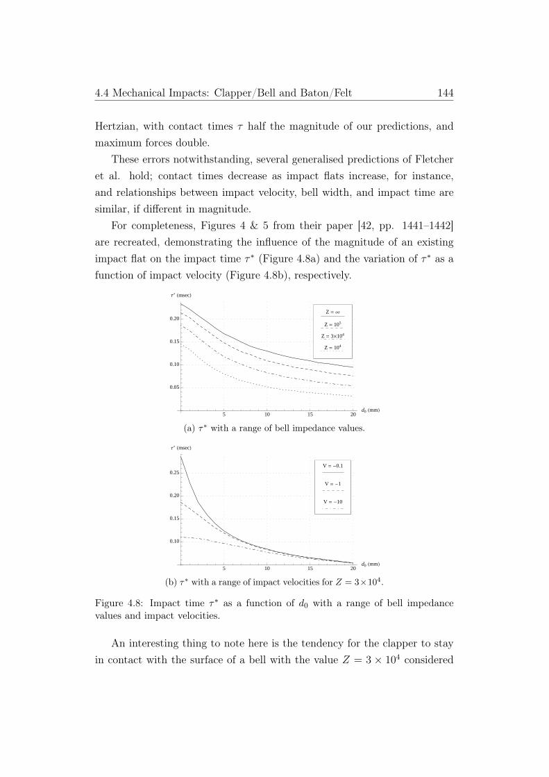
4.4 Mechanical Impacts: Clapper/Bell and Baton/Felt 144
Hertzian, with contact times τ half the magnitude of our predictions, andmaximum forces double.
These errors notwithstanding, several generalised predictions of Fletcheret al. hold; contact times decrease as impact flats increase, for instance,and relationships between impact velocity, bell width, and impact time aresimilar, if different in magnitude.
For completeness, Figures 4 & 5 from their paper [42, pp. 1441–1442]are recreated, demonstrating the influence of the magnitude of an existingimpact flat on the impact time τ ∗ (Figure 4.8a) and the variation of τ ∗ as afunction of impact velocity (Figure 4.8b), respectively.
Z = ¥
Z = 105
Z = 3´104
Z = 104
5 10 15 20d0 HmmL
0.05
0.10
0.15
0.20
Τ
* HmsecL
(a) τ∗ with a range of bell impedance values.
V = -0.1
V = -1
V = -10
5 10 15 20d0 HmmL
0.10
0.15
0.20
0.25
Τ
* HmsecL
(b) τ∗ with a range of impact velocities for Z = 3×10⁴.
Figure 4.8: Impact time τ∗ as a function of d0 with a range of bell impedancevalues and impact velocities.
An interesting thing to note here is the tendency for the clapper to stayin contact with the surface of a bell with the value Z = 3 × 10⁴ considered

4.4 Mechanical Impacts: Clapper/Bell and Baton/Felt 145
appropriate for bell 29 — a tendency which increases once d0 > 10 mm.Also, Figure 4.8b shows that impact time τ ∗ is quite sensitive to a rangeof clapper velocities with zero impact flat, but this sensitivity is lost, again,when d0 > 10 mm. This minimises the carillonneur’s ability to control thebell’s timbre through the variation of clapper velocity.
Contact Time Discrepancy
Figure 4.9 illustrates clapper motion and bell wall deformation for a rangeof values for d0. We see from 4.9c that a clapper with no impact flat isin contact with the bell wall until approximately 0.7 msec after impact, bywhich time the bell wall is maximally displaced.
d0 = 0
d0 = 5
d0 = 10
d0 = 15
0.2 0.4 0.6 0.8 1t HmsL
47.35
47.40
47.45
47.50
Hy1HtL + h0L HmmL
(a) Motion of the clapper’s centre of mass.
0.2 0.4 0.6 0.8 1t HmsL
-0.15
-0.10
-0.05
y2HtL HmmL
(b) Displacement of the bell wall.
0.2 0.4 0.6 0.8 1t HmsL
-0.04
-0.02
0.02
0.04
0.06
0.08
ΑHtL HmmL
(c) The approach, or the compression be-tween bodies; negative values describe thedistance between surfaces after contact.
Figure 4.9: Clapper, bell wall displacement and compression, y1, y2 and α respec-tively, during — and for a short period after — impact. Z = 3× 10⁴ with a rangeof initial flats up to d0 = 15 mm, equal to the impact flat on bell 29 prior tore-voicing.
These re-calibrated impact times allow an evaluation the second claim in

4.4 Mechanical Impacts: Clapper/Bell and Baton/Felt 146
Fletcher’s paper: that contact times predicted by the computations do notmatch those measured at the National Carillon. For bell 29, Fletcher et al.measured contact times of 0.6 msec for the damaged clapper (d0 = 15 mm)and between 1.0–1.2 msec for an undamaged clapper, considerably longerthan the contact times they predicted.
The re-calibrated model predicts contact times much closer to those mea-sured, although they still fall short for the undamaged clapper scenario, evenwith impedance Z = 3 × 10⁴ which exhibits the longest contact times. Solong, in fact, that for initial impact flats greater than 10mm, the clapper doesnot return from the bell, with those impacts having negative coefficients ofrestitution.
Figure 4.10 also plots the coefficient of restitution values (CORs) for thesame impact with Z = 105, showing them to be much larger. This variationseems to support Fletcher’s argument that Z is unrealistically sensitive aparameter for tuning theoretical results to match experimental data. Indeed,for Z < 2×10⁴ contact times become infinite, which also seems unrealisticallysensitive.
5 10 15 20d0 HmmL
0.1
0.2
0.3
0.4
0.5
eCoefficient of restitution
Figure 4.10: Computed coefficient of restitution for bell with Z = 3× 10⁴ (unbro-ken) and Z = 105 as a function of impact flat.
Further, Goldsmith provides a theoretical coefficient of restitution equa-tion based on contact time τ , plate depth b, striker mass m and materialproperties density ρ, modulus of elasticity E and Poisson’s ratio µ [55, p.

4.4 Mechanical Impacts: Clapper/Bell and Baton/Felt 147
2 4 6 8 10Z H´104L
0.2
0.4
0.6
0.8
CORCOR as function of Z
Figure 4.11: Coefficient of restitution from Goldsmith, from Eq. (4.58), with dif-ferent contact times: 0.47, 0.7, and 1 msec (dashed, unbroken and dot-dashed,respectively).
142]:
e =
πτb2(
Eρ
3(1− µ2)
)1/2
− 0.56m
πτb2(
Eρ
3(1− µ2)
)1/2
+ 0.56m
. (4.58)
which is also quite sensitive in the region 104 < Z < 5× 10⁴, and to contacttime (Figure 4.11).
Impact Times
The re-calculated force profiles require new determinations of the impacttimes τ ∗. Figure 4.12 gives the Fourier transforms for the impact forces withZ = 3× 10⁴ for the unvoiced and revoiced clappers.
The turnover frequencies f ∗ are quite different to those shown in Fletcheret al. (Figure 6, [42, p. 1442]), with the recalculated unvoiced and revoicedclappers having turnover frequencies of 2000 Hz and 1250 Hz, respectively,compared to 4000 Hz and 1800 Hz. Interestingly, the recalculated frequen-cies match up with with strong peaks in the sound spectrum they show; therevoiced clapper in particular, has a far stronger major 3rd tone at approxi-mately 1250 Hz, matching the f ∗ for the revoiced clapper in Figure 4.12b.

4.4 Mechanical Impacts: Clapper/Bell and Baton/Felt 148
f *
200 500 1000 2000 5000 1 ´ 104f HHzL
0.5
1.0
2.0
impulse
FHfL, d0 = 15
(a) Unvoiced clapper, f∗ ≈ 2 kHz.
f *
200 500 1000 2000 5000 1 ´ 104f HHzL
0.2
0.5
1.0
2.0
5.0
impulse
FHfL, d0 = 0
(b) Revoiced clapper, f∗ ≈ 1.25 kHz.
Figure 4.12: Fourier transforms of recalculated bell impact forces, with bellimpedance Z = 34.
Velocity of Bending Waves in the Bell
The group velocity of a transverse pulse in this material is twice that ofthe pulse velocity. Using the same equation for calculating pulse velocity asFletcher et al., from the analysis of Skudrzyk:
c =
(πZf
4M
)(4.59)
whereM is the bell mass per unit of area (≈ 121 Kg/m2) we can calculate groupvelocity by doubling the pulse velocity. Figure 4.13 plots the transverse pulsetransit times for the frequency range 1300–2000 Hz, and for different bellimpedances. As with the results in the previous section, these contact timesseem overly sensitive to bell impedance, although the results for Z = 5× 10⁴
(revoiced = 1.1 msec, and unvoiced = 0.85 msec) are a reasonably goodmatch for the measured times.
As noted in [42], Rossing [107] provides an alternate method of calcu-lating the flexural wave velocity, independent of the bell’s impedance. Thiscalculation is based on an analysis of the modes and frequency responses ofa bell and is roughly the mode’s frequency multiplied by the circumferencedivided by the number of modes, m:
v ≈ fdπ
m(4.60)

4.4 Mechanical Impacts: Clapper/Bell and Baton/Felt 149
1400 1500 1600 1700 1800 1900 2000f HHzL
0.6
0.7
0.8
0.9
1.0
1.1
1.2
1.3
msecPulse transit time
(a) Pulse transit times calculated from Sku-drzyk (Eq. (4.59)).
1400 1500 1600 1700 1800 1900 2000f HHzL
1.1
1.2
1.3
1.4
1.5
msecPulse transit times
(b) Pulse transit times calculated from Ross-ing (Eq. (4.60)).
Figure 4.13: Clapper pulse transit times as a function of frequency of maximumexcitation f∗, and different bell impedances Z = 3×10⁴, Z = 5×10⁴, and Z = 105
(unbroken, broken, dot-dashed) in (a).
where d is the bell’s diameter.Both of these equations return results in a similar range, but, as in
Fletcher et al., neither fully account for their experimental contact time mea-surements of 1.0–1.2 msec for the undamaged clapper, and 0.6 msec for thedamaged clapper. The impact-theory motivated equation Eq. (4.59) returnsa difference in contact times of only 0.25 msec from the undamaged to thedamaged impact, although a larger range of return times can be realised byadjusting the bell impedance. Rossing’s equation Eq. (4.60) returns a largerrange, closer to the difference reported by Fletcher et al., but the contacttimes are larger by about 0.5 msec for both scenarios.
Conclusion
The bell/clapper impact model, combined with a model for flexural wave ve-locity, returns contact times that are in reasonably good agreement with thetimes measured by Fletcher et al. [42], and others referenced in their paper.Without collecting separate measurements of this impact at the impact site,the re-calibrated model cannot be further verified. However, in the contextof the haptic model and the additional impact between the baton and thelower beam, there is some latitude for imperfect modelling. More importantthan contact times is the clapper’s motion after impact, and the simulations

4.5 Clapper and Baton Damper Impacts 150
performed using the re-calibrated model show that adjustment of the bellimpedance parameter can significantly alter this motion. This makes it anideal parameter for tuning simulated clapper motion.
4.5 Clapper and Baton Damper Impacts
4.5.1 Damper Impact Model
The rubber damper that prevents the clapper from travelling freely awayfrom the clapper is modelled in two parts, extending the formulation derivedfor the clapper/bell impact in the previous section.
In the clapper/bell impact, the bell wall was described by its impedanceonly; the model had no term for restoring the bell wall to its original position,partly because it was assumed that the flexural wave created at impact wouldtravel around the bell and provide a restorative force on return.
The surface of the damper (θd) is modelled using a first-order differentialequation which extends that for the surface of the bell given in Eq. (4.41c):
dθddt
= K(θ1min− θd)−
Fd(θ1, θd, p)
Zd(4.61)
with a boundary condition θd(0) = θ1min. TheK(θ1min
−θd) term is a constantforce internal to the rubber damper that tends to restore the rubber afterplastic deformation during impact.
The impact interaction force is modelled as a nonlinear spring; the extentof the nonlinearity is determined by the value for p:
Fd(θ1, θd, p) =
kd(θd − θ1)p if (θd − θ1) > 0
0 else(4.62)
The first term in Eq. (4.61) enacts the impact force inversely proportionalto zd, which encapsulates the extent of velocity-dependant plastic deforma-tion. This value can be thought of as the mechanical impedance of thedamper, as it approaches infinity the allowable deformation approaches zero.
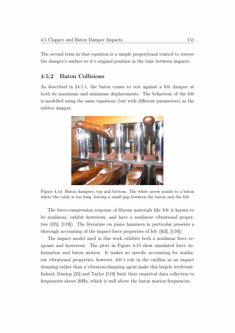
4.5 Clapper and Baton Damper Impacts 151
The second term in that equation is a simple proportional control to restorethe damper’s surface to it’s original position in the time between impacts.
4.5.2 Baton Collisions
As described in §4.1.1, the baton comes to rest against a felt damper atboth its maximum and minimum displacements. The behaviour of the feltis modelled using the same equations (but with different parameters) as therubber damper.
Figure 4.14: Baton dampers, top and bottom. The white arrow points to a batonwhere the cable is too long, leaving a small gap between the baton and the felt.
The force-compression response of fibrous materials like felt is known tobe nonlinear, exhibit hysteresis, and have a nonlinear vibrational proper-ties ([35], [119]). The literature on piano hammers in particular presents athorough accounting of the impact-force properties of felt ([63], [110]).
The impact model used in this work exhibits both a nonlinear force re-sponse and hysteresis. The plots in Figure 4.15 show simulated force de-formation and baton motion. It makes no specific accounting for nonlin-ear vibrational properties, however, felt’s role in the carillon as an impactdamping rather than a vibration-damping agent make this largely irrelevant.Indeed, Dunlop [35] and Taylor [119] limit their empirical data collection tofrequencies above 20Hz, which is well above the baton motion frequencies.

4.5 Clapper and Baton Damper Impacts 152
è
è
è
è
è
è
è
è
è
è
è
è
è
è
èè
è
è
è
è
è
è
è
è
èè
èè
èè è
èè è
èè
èè
è èèè
èèèè èèèèèèèèèè
èè
èèèèèèèèèèèèèèèèèè
èèèèèèèèèèèèèèèèèèèèèèèèèèèèèèèèèèèèèèèèèèèèèèèèèèèèèèèèèèèèèèèèèèèèèèèèèèèèèèèèèèèèèèèèèèèèèèèèèèèèèèèèèèèèèèèèèèèèèèèèèèèèèèèèèèèèèèèèèèèèèèèèèèèèèèèèèèèèèèèèèèèèèèèèèèèèèèèèèèèèèèèèèèèèèèèèèèèèèèèèèèèèèèèèèèèèèèèèèèèèèèèèèèèèèèèèèèèèèèèèèèèèèèèèèèèèèèèèèèèèèèèèèèèèèè
é
é
é
é
é
é
é
é
é
é
é
é
é
é
é
éé
éééé
é
é
é
é
é
é
é
é
é
é
éé
ééé
ééééééé
éé
éé
éé
éé
éééééé
éééééééééééééééééééééé
éééééééééééééééééééééééééé ééééééééééééééééééééééééééééééééééééééééééééééééééééééééééééééééééééééééééééééééééééééééééééééééééééééééééééééééééééééééééééééééééééééééééééééééééééééééééééééééééééééééééééééééééééééééééééééééééééééééééééééééééééééééééééééééééééééééééééééééééééééééééééééééééé
1 2 3 4
felt deformationHmmL0
10
20
30
40
50
60
70
Force HNLForce v. felt plastic deformation
(a) Force-deformation plot showing nonlinearforce response and hysteresis for repeated, im-pacts decreasing in velocity. • = loading, ◦ =unloading.
Τ
*
<
Τ
2» 0.033
Τ » 0.077
0.02 0.04 0.06 0.08 0.10t HsecL
10
20
30
40
50
60
70
NForce from felt compression
(b) Felt force during initial impact.0.00 0.02 0.04 0.06 0.08 0.10
t HsecL
1
2
3
4
mmBaton motion and felt deformation
(c) Felt deformation (broken line) and batonmotion during initial impact.
Figure 4.15: Force characteristics of the baton/damper impact simulation (batonvelocity = 0.2 m/sec).
A key part of carillon design is the combined role of the rubber damperand the felt-lined upper wooden beam on the clavier in stopping the clapperfrom travelling freely away from the inside of the bell wall. A finely-calibratedinstrument will have the impact load shared equally at the two sites; in prac-tice this cable tends to lengthen over time — it is not unusual, for instance,for the carillonneur to recalibrate over the course of a single recital [73].
Ideally, the turnbuckle is adjusted such that the baton at rest is lightlyin contact with the felt. If there is a gap between the baton and felt, the

4.5 Clapper and Baton Damper Impacts 153
clapper is being supported by the rubber damper alone. If the baton is toofirmly in contact with the felt, the baton is contributing too much to thesupport of the clapper. This relationship has consequences for the dynamicbehaviour of the entire mechanism, particularly when backlash in the batoncable is taken into account.
4.5.3 Cable Stiffness and Collisions
The following simulations demonstrate the role of cable stiffness and turn-buckle length in the dynamic behaviour of the carillon mechanism afterimpact. Because each of the individual impact sites (the bell, the rubberdamper, and both felt-lined beams on the clavier) are modelled using thesame formulation, the general results pertaining to the interaction betweenturnbuckle length and cable stiffness are relevant to collisions at both thebottom and top of the baton range.
Each of the following simulations replicates the data collection procedure.A force is applied at the baton tip sufficient to keep it at the bottom of itsrange. Once the mechanism has stabilised, this force is removed and thebaton returns to its rest position, rebounding several times with the upperbeam and eventually coming to rest.
With an ideal turnbuckle length, the baton’s maximum displacement willcorrespond precisely with the clapper’s maximum displacement as calculatedin the previous chapter; similarly their respective minimums will also align.In this situation, the entire carillon mechanism has a universal minimum andmaximum. This is not the case with a shortened or lengthened turnbuckle,which effectively shifts the baton and clapper ranges out of alignment. Thedynamic effect of this kinematic adjustment is explored in the following sim-ulations.
Stiff Cables (Uniform Velocity)
Figure 4.16 shows simulation results for baton motion, clapper motion, batondamper deformation and clapper damper deformation. The two dampersbegin the simulation at zero deformation. When the simulation begins, the
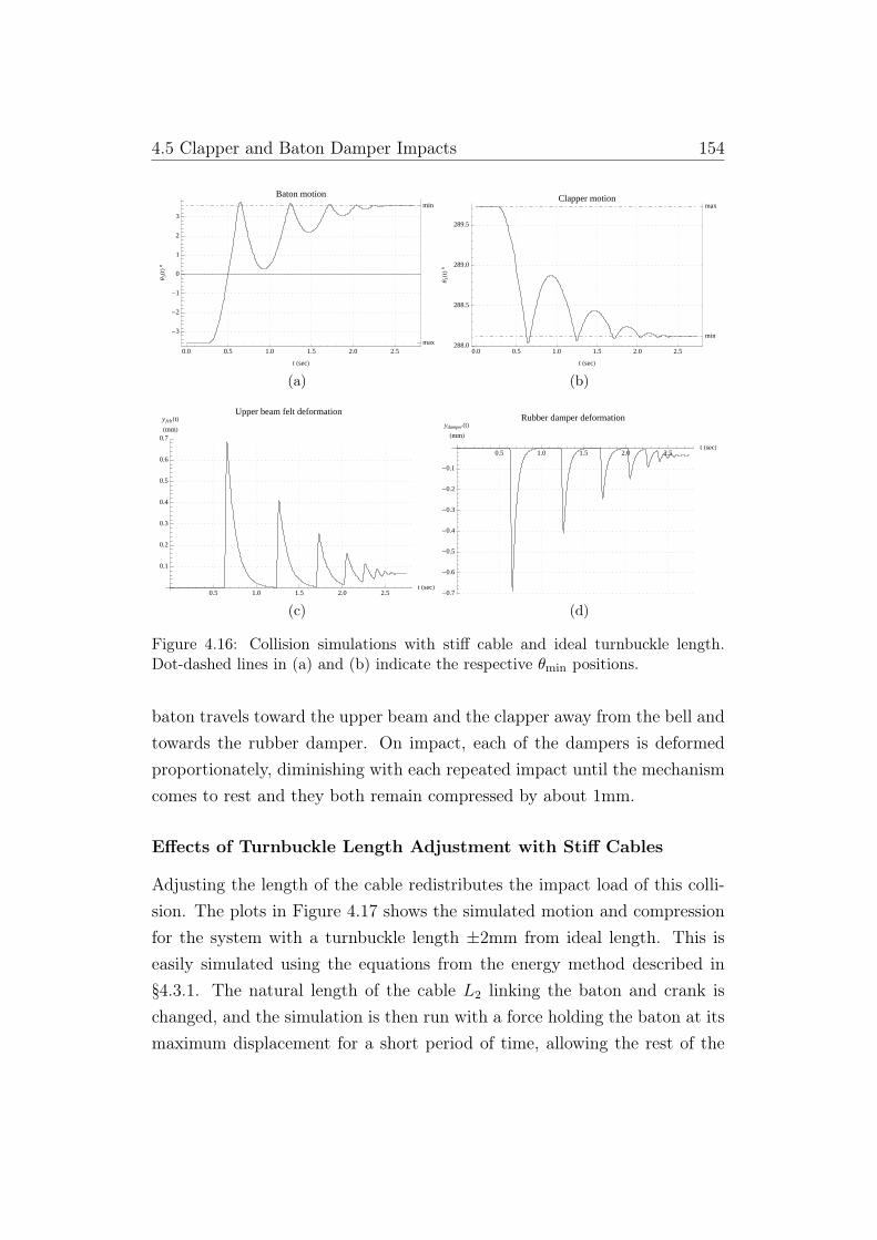
4.5 Clapper and Baton Damper Impacts 154
0.0 0.5 1.0 1.5 2.0 2.5
-3
-2
-1
0
1
2
3
min
max
t HsecL
Θ3
HtL°
Baton motion
(a)
0.0 0.5 1.0 1.5 2.0 2.5288.0
288.5
289.0
289.5
min
max
t HsecL
Θ1
HtL°
Clapper motion
(b)
0.5 1.0 1.5 2.0 2.5t HsecL
0.1
0.2
0.3
0.4
0.5
0.6
0.7
y feltHtLHmmL
Upper beam felt deformation
(c)
0.5 1.0 1.5 2.0 2.5t HsecL
-0.7
-0.6
-0.5
-0.4
-0.3
-0.2
-0.1
ydamperHtLHmmL
Rubber damper deformation
(d)
Figure 4.16: Collision simulations with stiff cable and ideal turnbuckle length.Dot-dashed lines in (a) and (b) indicate the respective θmin positions.
baton travels toward the upper beam and the clapper away from the bell andtowards the rubber damper. On impact, each of the dampers is deformedproportionately, diminishing with each repeated impact until the mechanismcomes to rest and they both remain compressed by about 1mm.
Effects of Turnbuckle Length Adjustment with Stiff Cables
Adjusting the length of the cable redistributes the impact load of this colli-sion. The plots in Figure 4.17 shows the simulated motion and compressionfor the system with a turnbuckle length ±2mm from ideal length. This iseasily simulated using the equations from the energy method described in§4.3.1. The natural length of the cable L2 linking the baton and crank ischanged, and the simulation is then run with a force holding the baton at itsmaximum displacement for a short period of time, allowing the rest of the

4.5 Clapper and Baton Damper Impacts 155
mechanism to settle into dynamic equilibrium. After a short period, the sys-tem is stable and we see a new relationship between the baton and clapper’srespective ranges.
0.0 0.5 1.0 1.5 2.0 2.5
-3
-2
-1
0
1
2
3
min
max
t HsecL
Θ3
HtL°
Baton motion, turnbuckle ± 2mm
(a)
0.0 0.5 1.0 1.5 2.0 2.5
288.0
288.5
289.0
289.5
min
max
t HsecL
Θ1
HtL°
Clapper motion, turnbuckle ± 2mm
(b)
0.5 1.0 1.5 2.0 2.5t HsecL
0.2
0.4
0.6
0.8
y feltHtLHmmL
Felt deformation, turnbuckle ± 2mm
(c)
0.5 1.0 1.5 2.0 2.5t HsecL
-1.4
-1.2
-1.0
-0.8
-0.6
-0.4
-0.2
ydamperHtLHmmL
Rubber damper deformation, turnbuckle ± 2mm
(d)
Figure 4.17: Collision simulations with stiff cable and variable (±2mm) turnbucklelength; unbroken lines = +2mm; dashed lines = -2mm.
The photograph in Figure 4.14 shows a baton with an over-long turn-buckle. This is indicated by the gap between the top of the baton and thefelt. We see this in the simulation in Figure 4.17. The unbroken line repre-sents the simulation of a turnbuckle +2mm longer than ideal, which wouldleave a 2mm gap between the baton and the felt, a little less than that inthe photograph. Around 2 seconds into the simulation, the system has cometo rest and the baton is around half a degree below its ideal resting placeagainst the felt (around 3.2 ◦, labelled ‘min’). The clapper is resting veryslightly past θ1min by a distance proportional to the rubber damper defor-mation, which is about 0.25mm. At this point, the clapper load is wholly
4.5 Clapper and Baton Damper Impacts 156
supported by the clapper’s damper.The opposite is the case when the turnbuckle is shortened (broken line in
plots). The clapper’s damper is negligibly deformed (Figure 4.17d) and theupper beam felt remains deformed when the system comes to rest at about2.5 sec.
There is an additional dynamic consequence of a poorly adjusted turn-buckle, arising from an altered maximum clapper position. The clapper mo-tion plot in Figure 4.17 shows a 0.2 ◦ difference in the clapper start positions,even though the baton position for both simulations is at the same position,at the bottom of its stroke. As the baton is released, the dashed (turnbuckle= −2mm) clapper/baton pair easily beat the unbroken pair to impact, eventhought the unbroken clapper had less distance to travel.
This is a result of the lower force resulting from the clapper’s mass atan angle and gravity: the clapper with a lower maximum angle has lessgravitational force acting on it that the other clapper, resulting in a differenceof about 50 msec to impact with the other clapper.
Effects of Turnbuckle Length Adjustment with Spring Cables
Running these simulations with a more realistic cable model heightens the in-fluence of different turnbuckle lengths. When the turnbuckle is shortened by2mm, the clapper’s damper comes into play because the cables will increasein length on impact, increasing the net amount of deformation possible. InFigure 4.18, the damper is deformed by 1mm compared to the near-zerodeformation in the previous simulation with stiff cables (Figure 4.17d).
This has a noticeable effect on the amount by which the clapper andbaton return after impact, and the length of time the system remains inmotion. The baton motion plot in Figure 4.18a, for instance, shows thebaton returning below the mid-point of its stroke, and only really coming torest after 3.5 seconds; the same simulation with stiff springs in the previousFigure 4.17a has the baton coming to rest after two seconds, and not reachingthe mid-point after the first impact.
The cables modelled as virtual springs introduce another dynamic feature

4.5 Clapper and Baton Damper Impacts 157
0.0 0.5 1.0 1.5 2.0 2.5 3.0 3.5
-3
-2
-1
0
1
2
3
min
max
t HsecL
Θ3
HtL°
Baton motion, turnbuckle ± 2mm
Hcable stiffnes = 105N�mL
(a)
0.0 0.5 1.0 1.5 2.0 2.5 3.0 3.5
288.0
288.5
289.0
289.5
min
max
t HsecL
Θ1
HtL°
Clapper motion, turnbuckle ± 2mm
Hcable stiffnes = 105N�mL
(b)
0.5 1.0 1.5 2.0 2.5 3.0 3.5t HsecL
0.1
0.2
0.3
0.4
0.5
y feltHtLHmmL
Felt deformation, turnbuckle ± 2mm
Hcable stiffnes = 105N�mL
(c)
0.5 1.0 1.5 2.0 2.5 3.0 3.5t HsecL
-2.0
-1.5
-1.0
-0.5
ydamperHtLHmmL
Rubber damper deformation, turnbuckle ± 2mm
Hcable stiffnes = 105N�mL
(d)
Figure 4.18: Collision simulations with loose cable and variable (±2mm) turnbucklelength; unbroken lines = +2mm; dashed lines = −2mm.
characteristic of the baton in motion: a jittery rather than smooth motionthat results from friction in the mechanism. The largest source of friction inthe entire mechanism is the static and dry friction resulting from the felt-linedbaton rubbing against the metal bars on either side. A non-rigid cable modelallows this friction to retard the baton motion by acting on the dynamics ofthe baton separately to the dynamics of the rest of the mechanism. A slightincrease in jitter can be discerned in the baton motion measurements plottedin the next chapter.
4.6 Summary 158
4.5.4 Conclusion
The more accurate cable-as-spring model allows for the fine-tuning of batonmotion depending on turnbuckle length and the slackening of the cable duringsome impacts. The simulations exploring the influence of turnbuckle lengthcorrespond with experiences at several carillons, particularly a perceivablesluggishness in batons with over-long turnbuckles. The stiff cable model alsocaptures this behaviour, but with less sensitivity to turnbuckle length. Inboth models turnbuckle length is the parameter with most influence on thefree motion of batons after impact with the upper beam, although it hassignificantly less influence on the force-feedback of a baton, particularly inhigher bells where gravity acting on the clapper mass contributes less to thedynamics of the baton.
4.6 Summary
This chapter has developed two dynamic models for the carillon mechanism.The uniform velocity model is a linearisation based on the simplificationthat the three subsystems rotate over a very small range, and that the cableslinking them are inextensible rods fixed at unchanging angles to the respectivesystems. The second model incorporated the cables as springs that exert forcewhen expanded. This more accurate model also allowed for independentmotion between systems during impacts, as well as the subtle changes inangles between cables and the rotating systems. A limited verification of thetwo models was performed by comparing their motion in response to a staticapplied force, and no force.
The linearised model simplifies parameter estimation in the followingchapter. It is also used to modelling the change in force-feedback acrossthe entire carillon in later user-testing, where continuous models of parame-ter variation are used to populate the linear model for haptic display, withoutconcern for deviations in the behaviour of individual batons. The virtual-spring model is used for offline simulation of individual batons, and is alsoappropriate for online simulation of batons that exhibit behaviour that can-

4.6 Summary 159
not be replicated with the linear model like the dramatic variation in batonmotion due to changing turnbuckle lengths.

Chapter 5
Implementation of the HapticModel
The set of equations developed over the course of the previous chapter formsa virtual carillon model which describes the motion and force interactions ofa carillon mechanism; specifically, they are arranged to simulate the motionof a baton in response to carillonneur-applied force. This forward dynamicssimulation is combined with a servo controller and a linear actuator coupledto a manipulandum (a wooden baton) to form an admittance display schemewhich produces baton motion in response to measured carillonneur force.
A commercial position-control servo and linear actuator system is usedfor controlling the kinematic state of the baton, and user-applied force ismeasured by monitoring the noisy force commands from the servo to theactuator. A theoretical model of the servo/actuator system is developed,and forms the basis of a Kalman filter for filtering this noisy signal.
5.1 Admittance Control
In the admittance control scheme, the kinematic state of the manipulandumis determined by the dynamic virtual environment and force inputs to thatenvironment. These forces are applied by the user at the manipulandum andsensed by a force sensor. The dynamic environment calculates new velocity
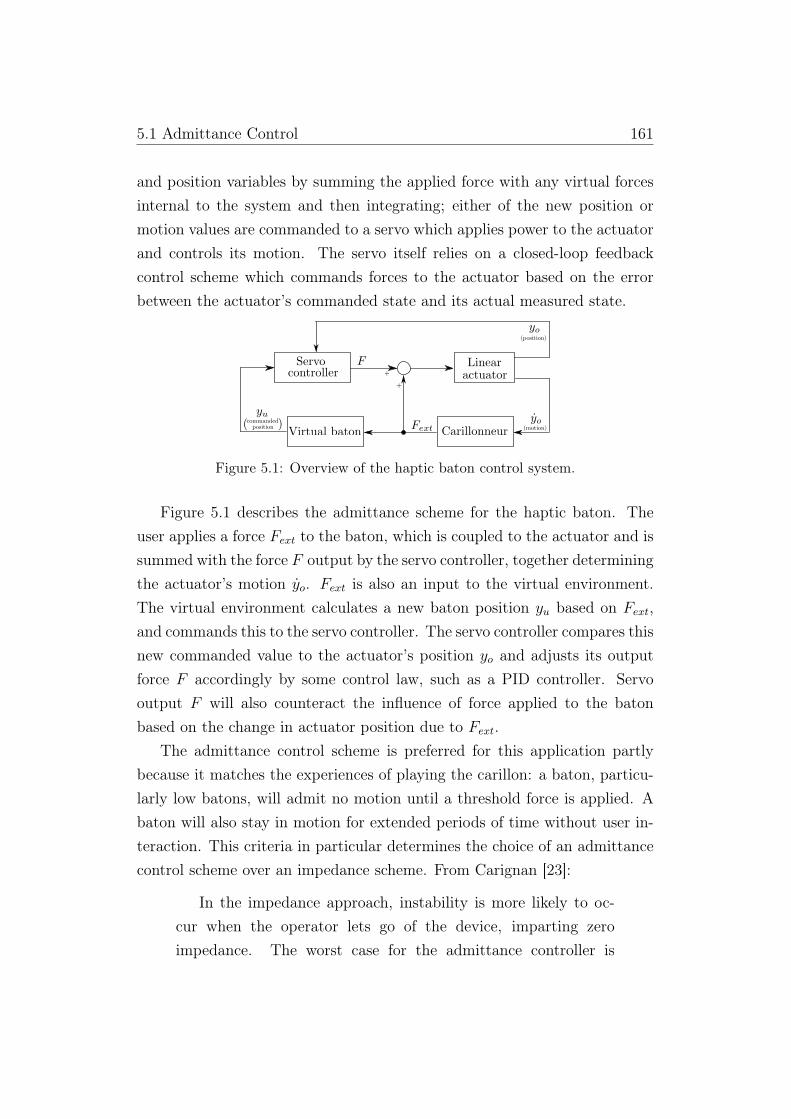
5.1 Admittance Control 161
and position variables by summing the applied force with any virtual forcesinternal to the system and then integrating; either of the new position ormotion values are commanded to a servo which applies power to the actuatorand controls its motion. The servo itself relies on a closed-loop feedbackcontrol scheme which commands forces to the actuator based on the errorbetween the actuator’s commanded state and its actual measured state.
+
+
Figure 5.1: Overview of the haptic baton control system.
Figure 5.1 describes the admittance scheme for the haptic baton. Theuser applies a force Fext to the baton, which is coupled to the actuator and issummed with the force F output by the servo controller, together determiningthe actuator’s motion yo. Fext is also an input to the virtual environment.The virtual environment calculates a new baton position yu based on Fext,and commands this to the servo controller. The servo controller compares thisnew commanded value to the actuator’s position yo and adjusts its outputforce F accordingly by some control law, such as a PID controller. Servooutput F will also counteract the influence of force applied to the batonbased on the change in actuator position due to Fext.
The admittance control scheme is preferred for this application partlybecause it matches the experiences of playing the carillon: a baton, particu-larly low batons, will admit no motion until a threshold force is applied. Abaton will also stay in motion for extended periods of time without user in-teraction. This criteria in particular determines the choice of an admittancecontrol scheme over an impedance scheme. From Carignan [23]:
In the impedance approach, instability is more likely to oc-cur when the operator lets go of the device, imparting zeroimpedance. The worst case for the admittance controller is

5.1 Admittance Control 162
when the operator grasps the handle tightly, imparting maximumimpedance.
In a performance context, the carillonneur will never grasp the handle of thebaton, and will apply force to the playing end of the baton from above. In arehearsal context, it is possible that the carillonneur will grip the baton whilstacclimatising to its force-feedback, but will minimise their own impedanceprecisely because they are trying to gauge the impedance characteristics ofthe baton.
The other aspect of admittance control which raises stability issues isthe magnitude of the virtual mass being modelled. As noted by Haywardand Maclean [66], an admittance controller must have high gain feedbackin order to move freely, “the device must be capable of high acceleration inresponse to measured user forces”. Seeing as the inherent mass and dampingof the actuator is fixed, this introduces requirements relating to virtual mass,damping and the quality of force sensing. However, the nature of this limi-tation further suits the carillon prototype: the virtual mass being modelledis always relatively large, and the virtual mechanism is significantly dampeddue to the large number of frictional elements.
Adams and Hannaford confirm this in their study of stable haptic systems[1], and make the further point that the stability of a haptic interface canbe manually tuned when the virtual environment is known ahead of time.Virtual coupling between the haptic device and the virtual environment toguarantee stability is unnecessary in this application, and analytically prob-lematic because the operation of the servo controller is not fully known.
5.1.1 Hardware
A commercial electromagnetic voice-coil linear actuator and analog servosystem, originally designed as a kinaesthetic complement to car stereo sys-tems, was chosen for the development of the haptic baton. It has a 1.5 cmdisplacement, and can provide a continuous force of about 90 N across the en-tire displacement length. A position sensor is incorporated into the actuatorcasing, and combined with the servo the actuator can reproduce frequencies

5.1 Admittance Control 163
up to 10 kHz.
(a) Electromagnetic linear actuator
(b) Servo controller
Figure 5.2: Electromagnetic linear actuator and servo controller
The stroke/armature component has a mass of 0.48 Kg. The armatureis encased in a hard plastic cylinder, which is itself enclosed by a cylindricalcoil which constitutes the outer body of the actuator. The plastic cylinderand coil are in thinly-lubricated contact with each other, and there is a clearsensation of static friction and dry friction when in an unpowered state.Informal experimentation puts the value of static friction at about 5 N, thisvalue is used as an initial guess in later parameter identification processesapplied to the entire system.
The servo controller has force and position inputs, and outputs which

5.2 Force Sensing 164
report the measured actuator position and the current being sent from theservo to the actuator. When this measurement is taken it has already beenconverted to a voltage ±5.5 onboard the servo, and the resistance in thisconversion circuit is not known. Therefore, although the term ‘current signal’is used in this chapter, the measurements are given in N by an empiricallydetermined force/voltage constant.
The combination of high-frequency position-control and force character-istics is ideal for this carillon application, which requires quick gestures andfirm force-feedback. Further, the large stroke mass and damping internal tothe actuator lowers the theoretical virtual mass and damping limit for anadmittance control scheme [83]; later in this chapter, the full prototype isdemonstrably stable in a rotational mass-spring-damper simulation with avirtual inertia of 0.05 kg ·m2 and virtual damping of 0.2 N.m/(rad/sec).
5.2 Force Sensing
Fitting a zero-offset straight line to a series of static measurements showsour device to have a force/voltage constant of 41.9 N/V. The measurementsand linear fit are shown in Figure 5.3.
ò
ò
ò
ò
ò
ò
ò
ò
0.2 0.4 0.6 0.8 1.0 1.2
measuredvoltage HVL
10
20
30
40
50
applied forceHNL
Servo output force�voltage relationship
Figure 5.3: Servo force/voltage relationship. Eight static forces were applied tothe actuator and the servo current output (converted internally to voltage) wasmeasured. A straight line y = 41.9 was fit, giving force/voltage.
The plots in Figure 5.4 show the extent to which noise contaminates thecurrent signal. A 15 second sample was recorded during which force wasrepeatedly applied directly to the actuator’s stroke. During periods where

5.2 Force Sensing 165
no force is applied by the user (0–2 sec; 12–15 sec), there is a constantexternal force which is the product of gravity acting on the stroke’s mass.The covariance in these periods is about 10 N. During the period 6–10 seca near-constant user-applied force of approximately 20 N is applied, and theerror covariance increases dramatically to almost 40 N.
Figure 5.4d plots the actuator stroke position recorded from the servooutput. The noise in this signal is also contributes to servo process noise,as it is known that the servo relies on this signal to control the actuator’sposition.
Filtering this force signal should attenuate the high-amplitude, high-frequency control transients whilst preserving transients which are producedin response to user-applied force, or disturbances; developing a model forthese control transients will help isolate those disturbances.
2 4 6 8 10 12 14sec HtL
-60
-40
-20
20
NMeasured force to actuator, sampling rate = 1kHz
(a) The full 15 second sample.
0.05 0.10 0.15 0.20 0.25 0.30 0.35sec HtL
-15
-10
-5
5
10
15
20
NMeasured force to actuator
(b) Sample period with no user-applied ex-ternal force.
2.1 2.2 2.3 2.4 2.5 2.6 2.7sec HtL
-60
-50
-40
-30
-20
-10
NMeasured force to actuator
(c) Gradually applied external force.
2 4 6 8 10 12 14t HsecL
-2.0
-1.5
-1.0
-0.5
0.5
1.0
mmMeasured actuator position, sampling rate = 1kHz
(d) Measured actuator stroke position.
Figure 5.4: Unprocessed force measurements from current to actuator, and positionerror during applied external force.

5.3 Modelling the Servo and Actuator for Kalman Estimation 166
5.3 Modelling the Servo and Actuator for
Kalman Estimation
In the case of a black-box robotic system, it has been shown that stochasticfiltering based on time-series ARIMA models forecasting future values is asuitable method for force sensing [89] [82].
However, the servo controller and actuator need not be considered a black-box system. Using system identification and parameter estimation tools, itis possible to develop and fit a theoretical model describing the behaviour ofthe system bounded by the application requirements. This model consistsof a servo controller operating on position/position-error and a nonlinearactuator model. The application requirement is to find a servo model thatresponds to user disturbance with a force proportionate to that disturbance,not necessarily a servo model that matches the noisy force output.
The linear servo controller portion of this model can then be extracted toform the basis of a Kalman estimator, which treats unknown control tran-sients as measurement and process noise. The Kalman estimator has deter-ministic (measured position) and stochastic (servo output force) inputs, andoutputs an estimated force that more accurately reflects that applied by theuser.
Kalman Estimation
The discrete-time linear Kalman estimator is a recursive algorithm for esti-mating the state of a linear dynamic system whose process is perturbed bynoise, using measurements that are corrupted by uncorrelated noise. Theestimator minimises the covariance of the error between a system’s state andan a posteriori estimated state. This a posteriori estimate is based on aweighted linear combination of an a priori state estimate and the differencebetween a measurement prediction based on this state and an actual noisymeasurement of the system. This difference is referred to as the residual.
This weighting is determined by the Kalman gain, which effectively de-termines the balance of trust the estimator puts in the predicted state versus

5.3 Modelling the Servo and Actuator for Kalman Estimation 167
the noisy measurements. Calculation of the Kalman gain depends on someuser-supplied estimates of measurement and process noise covariance, whichmeans it can be tuned to different application requirements. Clappers nearthe top of the carillon range, for instance, respond to small changes in force,so minimising noise in the force signal will be a priority, which can be achievedby placing more trust in the state estimate. The dynamics of a low clapperare not as susceptible to small changes in force, so the estimator could beoptimised instead for aggressively accepting changes in measured force, evenif this means a slightly higher noise covariance.
The Kalman estimator requires some knowledge of the dynamics of thesystem being estimated, and the performance of the estimator as a filterwill depend on how well that process is modelled. In this application, theKalman estimator has its own copy of the process being modelled (the servocontroller) which it will use to estimate a new state based on the controlinput (position error) and the actual output of the process (force outputfrom the servo to the actuator). Figure 5.5 presents an overview of thisprocess; mathematical references are given later in this section.
Figure 5.5: Kalman filtering of servo force output. An a priori estimate is basedon the previous state estimate xk−1 and control input uk−1. This estimate is thensummed with a Kalman gain weighted residual Kk(zk −Hx
−k ) to create an a pos-
teriori state estimate. The filtered force is extracted using the state measurementmatrix H.
The Kalman estimator is ideal for this application, where it is difficultto construct an accurate model of the servo, but one can be designed thatweights responsiveness to position error over accuracy of state estimate. Inthis respect, it is possible to model for desirability of system behaviour ratherthan accuracy: the Kalman estimator will reconcile imperfect state estimateswith noisy data, correcting internal state estimates but favouring quick re-

5.3 Modelling the Servo and Actuator for Kalman Estimation 168
sponse.
5.3.1 Servo and Actuator Model
A typical servo controller for position control will have some linear controlleroperating on the error between the commanded and observed position (posi-tion loop), and some form of friction compensation operating on the observedor calculated velocity (velocity loop). Whilst the linear controller operatingon the position loop is likely to be a PI or PID controller [76], the frictioncompensation scheme is less-reliably estimated due to the large number ofavailable techniques (see [96]) alongside the varied techniques for velocityestimation based on measurements from displacement sensors [133].
-+
+
+
Figure 5.6: Sampling position and force outputs. The bounded portion of themodel is expanded in Figure 5.7.
Figure 5.6 shows the inputs and outputs of the servo and actuator model.The sampled position error and force outputs can be related to the Kalmanfiltering diagram above in Figure 5.5. The Kalman filter takes position er-ror as the deterministic input; this error is calculated by subtracting themeasured position at time k with the commanded position at time k − 1.Force output at time k is the stochastic input, and this is combined with thepredicted state output to create a more accurate state estimate.
Two servo controller models are evaluated: a PID operating on positionerror, and a PI operating on position error along with a velocity loop calcu-lated by taking the derivative of measured position. This serves as both asanity check on the values returned from the parameter estimation procedure,and a basis for comparing the role different components play.

5.3 Modelling the Servo and Actuator for Kalman Estimation 169
Both models leave a possible unknown function in the real servo con-troller unmodelled. The nature of the oscillations in the force signal hintthat this unknown function might be some form of dither signal, a techniquefor supplying extra forces to the actuator which keeps it in motion to avoidthe effects of stiction [96], [102]. Measurement noise in the position signalwill also contribute to oscillations in the force signal.
Servo Controller Model — PID
Figure 5.7a shows the hypothesised servo controller comprising a linear com-ponent CPID(s) and an unknown function contributing unmodelled processnoise Ff .
The transfer function for the parallel PID controller is the sum of theindividual components
CPID(s) =F
ye= Kp +
Ki
s+KdDNs
s+DN
=KiN + s(Ki +KpDN) + s2(KdDN +Kp)
s(s+DN)(5.1)
with an output force F to input error ye, and where Kp is the proportionalgain, Ki is the integral gain, Kd is the derivative gain, and DN is the locationof the derivative filter pole.
The servo controller outputs a force F to the actuator, which is summedwith the force Fext applied by the user. This summed force Ftot acts on theactuator stroke, creating an error between the commanded position and itsactual position.
Servo Controller Mode — PI with Velocity Feedback (PIV)
An alternate model for the servo controller has a linear PI controller CPI(s)operating on the error signal ye from which with a velocity feedback gainthat is based on a filtered derivative of the position signal is subtracted. Theentire multi-input (position error ye, and position yo) single-output (servo

5.3 Modelling the Servo and Actuator for Kalman Estimation 170
++
+
+
+
+
-
++
+
-
(a) Servo controller as PID on error ye.
++
+
+
+
-
+
+
+
- -
(b) Servo controller as PI on error ye with velocity feedback Fvel derived from yo.
Figure 5.7: Hypothesised servo controller and actuator models. Servo force to theactuator F and stroke displacement yo are sampled to get Fk and yek−1
as inputsfor later filtering.
force F ) PIV model is then described by the following transfer functions:
CPIV (s) = CPI(s)−Hvel(s)
CPI(s) =FPIye
= KPI
(Kp +
Ki
s
)Hvel(s) =
Fvelyo
=KvVns
s+ Vn(5.2)
The velocity gain has the same form as the derivative component in thePID controller, with Kv being the velocity gain, and VN locating the deriva-tive filter pole.

5.3 Modelling the Servo and Actuator for Kalman Estimation 171
Actuator Model
The motion of the actuator’s stroke is governed by the equation
myo + ffric(yo) = Ftot (5.3)
where ffric is a nonlinear frictional function, modelled here as a combinationof viscous, Coloumbic and Stribeck friction with an adjustment to remove thediscontinuity associated with Coloumbic friction and stiction when velocitychanges direction [96]. In this model, there is a small but finite region oflinear friction when velocity is below a threshold, vth, with values typicallybetween 10−3 and 10−6 m/s (see [5]).
ffric(yo) =
(Fc + (Fbrk − Fc)e−|yo/vs|
)sign(yo) + Fvyo if |yo| >= vth
yoFvvth + (Fbrk − Fc)e−vsvth)
vthif |yo| < vth
(5.4)
-1.0 -0.5 0.5 1.0y
oHm�sL
-15
-10
-5
5
10
15
ffric HNLActuator friction model ffricHy oL
(a) Friction force for −1 < yo < 1 m/s.
-0.010 -0.005 0.005 0.010y
oHm�sL
-10
-5
5
10
ffric HNLActuator friction model ffricHy oL
(b) Linear portion of friction model.
Figure 5.8: Output of the actuator friction model described in Eq. (5.4) for valuesidentified in for PID (unbroken line) and PIV (dashed line) models (Table 5.1).Difference between the models is given by the dotted line.
In this above equation, Fv is the linear friction associated with viscousfriction, Fc is the constant Coloumbic friction, and Fbrk determines the mag-nitude of stiction with Stribeck velocity vs controlling the rate at whichfriction force decreases after a change in velocity direction before increasingagain as velocity increases.

5.3 Modelling the Servo and Actuator for Kalman Estimation 172
The PID controller responds to this error with a force rejecting the ex-ternal disturbance. However, the servo output will also contain forces over-coming the physical characteristics of the actuator itself, like inertia andfriction which become especially significant when the actuator is in motion.These physical characteristics need to be modelled in order to identify servoforces attributable to overcoming them from the measured force signal, andremoving them to leave the servo force component dealing with external dis-turbances.
5.3.2 System Identification
Table 5.1: System identification results for servo and actuator parameters, PID,PIV, PI and PIVK(developed in §5.3.3) models (∗ = known; � = manually ad-justed).
Value
Parameter PID PIV PI PIVK
m* (Kg) 0.48 0.48 – –Fc (N) 7.5 6.1 – –Fbrk (N) 10 9.6 – –Fv (N/(m/s)) 9 4.8 – –vs (m/s) 0.1 0.1 – –vth* (m/s) 10−3 10−3 – –Kp 12695 20924 12000� 12000�
Ki 2152 2407 1250� 1250�
Kd 860 – – –DN 2470 (100�) – – –Kv – 401 – 25�
VN – 320 – 500�
KPI – – 1.3� 1.3�
A linear chirp signal with a frequency going from 0.5–10 Hz over 15 sec-onds and an amplitude set to the actuator’s maximum stroke was commandedto the servo, and the actuator position and servo force output was recorded.Two Simulink models of the servo and actuator system simulating PID andPIV controllers were then constructed, along with a parameter estimation en-

5.3 Modelling the Servo and Actuator for Kalman Estimation 173
vironment to find numeric values associated with the actuator and respectiveservos.
Using the Matlab Pattern Search estimation method, the parameter es-timation task was defined so as to find numeric values for the servo andactuator friction parameters that minimised the sum of squares error (SSE)between the simulated actuator position response and the measured positionresponse. Table 5.1 lists these numeric values.
The estimated actuator parameters for both models are reasonably close— the difference in viscous friction Fv does not result in a large divergencebecause the velocities in the signal are quite low, the maximum being justover 0.6 m/s. The difference in Coloumbic friction Fc has more influenceon the shape of the velocity-force curve in Figure 5.8a, where the error is3N by yo = 0.5 m/s; taking into account the mechanical advantage whenthe actuator is coupled to the baton, this corresponds to a baton strokecovering its entire displacement in around 40 msec, which is well beyond theapplication requirements.
PID Results
Plugging the values found for the PID controller into the Simulink model andcomparing the simulated motion with that measured shows the goodness ofthe fit for position error. No meaningful deviation is observed when plottingone on top of the other (Figure 5.9a), and the residuals are small (Figure5.9b).
However, this model is almost certainly not accurate. Aside from theperiodicity in the residuals, which indicates some systematic problem withthe PID model, the simulated force output to the actuator (Figure 5.9c) iswildly different from the measured force (Figure 5.11a).
The simulated force is smoother than the measured force; this is ex-pected because the model makes no attempt to model the noisy parts of theservo force. A far greater difference is seen in their respective magnitudes.The simulated force reaches close to 2000 N while the measured force barelyreaches 60 N. An analysis of the contribution of the individual proportional,

5.3 Modelling the Servo and Actuator for Kalman Estimation 174
2 4 6 8 10 12 14t HsecL
-6
-4
-2
2
4
6
y0 HmmLMeasured and simulated chirp response HPIDL
(a) Simulation and measured positions
2 4 6 8 10 12 14t HsecL
-0.1
0.1
0.2
0.3
mmResiduals from measured and simulated chirp HPIDL
(b) Position residuals
2 4 6 8 10 12 14t HsecL
-2000
-1000
1000
2000
NSimulated force for chirp signal HPIDL
(c) Simulated force output
2 4 6 8 10 12 14t HsecL
-60
-40
-20
20
40
60
NSimulated PID force DN = 100
(d) Simulated force output with diminishedDN = 100.
Figure 5.9: PID system identification results for chirp signal commanded to servoand actuator.
integral, and derivative components shows that the derivative component isalmost entirely responsible for the large forces.
Changing the derivative filter value DN from the estimated 2470 to amanually-adjusted 100 dramatically reduces the force magnitude, bringing itin line with the measured force, and also introduces some oscillatory noise(Figure 5.9d). This change increases the residuals between the measuredand simulated position, and is a poorer fit than the estimation. However, wewill adopt this change in the model because matching servo force output isprioritised over minimising position residuals.
PIV Results
Simulation of the PIV model with estimated parameters from Table 5.1 givesa position response very similar to the PID model; the results are plotted

5.3 Modelling the Servo and Actuator for Kalman Estimation 175
in Figures 5.10a. The residual plot shows an improved error during thelow velocities at the beginning of the sample, and the force output of theestimated PIV model is much closer to the measured force (Figure 5.11a), andof a similar shape to the PID simulation with manually adjusted derivativevalue (Figure 5.9d).
2 4 6 8 10 12 14t HsecL
-0.10
-0.05
0.05
0.10
0.15
mmResiduals from measured and simulated chirp HPIVL
(a) Position residuals.
2 4 6 8 10 12 14t HsecL
-60
-40
-20
20
40
60
NSimulated force for chirp signal HPIVL
(b) Simulated force output.
Figure 5.10: PIV system identification results for chirp signal commanded to servoand actuator.
5.3.3 Force Comparison and Tuning the Estimate
The system identification and parameter estimation procedure has returnedtwo possible candidates for the servo control: the PID system with amanually-adjusted derivative pole DN ; and the PIV system as estimated.The parameter estimation sought to minimise the error between measuredand simulated position, however of greater interest to us is the extent towhich the simulated force matches that measured from the servo.
In the first part of this subsection, the force outputs for the simulatedchirp signal used for parameter estimation are compared with the measuredsignal. This will determine how accurately forces due to actuator motion canbe filtered from a measured signal prior to, or after, Kalman filtering.
In the second part, a new force signal is recorded from the servo. Thissignal is in response to a constant position command and a gradually appliedforce. The position signal is also recorded and used as an open loop inputto the servo model. This demonstrates the extent to which the servo models

5.3 Modelling the Servo and Actuator for Kalman Estimation 176
can accurately simulate the force output in response to position error alone,avoiding the dynamics of the actuator itself, and this refinement of the modelbecomes the basis of the Kalman state estimation.
Response to Chirp Signal
2 4 6 8 10 12 14t HsecL
-60
-40
-20
20
40
60
NMeasured force for chirp signal
(a) Measured servo force.
åååå
åå åååååå
ååååååååååååååå ååååååååååååååååå åå å ååååååååååååååååå å å å ååååååååååå ååååå
å
å
å
å
å
ååå
ååå
å
åååå
ååååååå
å åååå
ååååååååååååååå åååååååååååååååååå å åå å åååå
åååååååååååå
åå å å å å åååååååååååå
åå å å å
å
å
å
å
å
åå
å
åå å
å
ååå
åå å å
åååååååå
ååååååå
åååååå ååååååååååååååååååå ååååååååååååååååååå å åå ååååååååååå ååååå å å å å ååå
å
å
å
å
ååå
ååå
å
ååå
åååå
åååå
ååååååååååååå åååååååååååååååååå
ååå å åååååååååååååå
åå åå å åå å åååååååååååååå å å å å å åå
å
å
å
åååå
å å åå åå
ååå å åååå
åååååååååååååå åååååååååååååååååååå åååååååååååååååååå å å åå åååååååååå åå å ååå å å å å ååå
å
å
åå
å
ååå
ååå
å
ååå
ååå
åå
åååååå
åååååå
ååå åååååååååååååååååå åå å å ååååå
ååååååååååå åå å å å åååå
ååååååååååå å å å å å
å
å
å
å
å
åå
å
åå å
å
åååå
å å ååååååååå
åååååååå
ååå ååååååååååååååååååå å åååååååååååååååååå å åååååååååååå åååååå å å
å
å
å
å
å
åå
å
ååå
å
åååå
ååååååå
ååååå
åååååååååååå åååååååååååååå
ååååå å å å ååååååååå
ååååååå
ååå åå å åå
ååååå åååååå
å
å
åå
å
å åå
åå å
å
åååååå
åå
ååå å ååååååååååå
åååååååå å ååååååååååååååååå åå åååååååååååååååååå å å åå åååååååååå
å
å
åå
å
å åå
ååå
å
ååå
ååå
åå
åååååååå åååååååååååååååååå å å åååååå
ååååååååå
åååå å å å åå
åååå
ååååååååå
å å å å å å åå
å
å
å
å
å
åå
å
åå å
å
åååå
å å ååå
ååååååå
ååååååååååååååååååååååååå åå å ååååååååååååååååå å å å ååååååååååååååååå
å
å
å
å
å
åå
å
åå
å
å
ååå
ååå
å
ååå
ååååå
ååååååååååååååå å ååååååååååå
åååååå
å å å å ååååå
ååååå åå
åååå
å å å å åååååååå
å
å
åå
ååå
åå å
ååååå
ååå
åååååååååååå åååå
åååååååååååååååå åååååååååååååååååå åå å ååååååååå å ååååååå å å å
å
å
åå
å
ååå
ååå
å
åååå
ååååååååååå
ååååååååååå å å åååååååååååååååå
å åå å åååååååååå
åååååå
å å å å å å ååååååå
å
å
å
å åå
åå å å å åå
åååååååå
ååååååååå ååååååååååååååååååå å åååååååååååååååååå å å å åååååååååå ååååååå å
å
å
å
å
å
åå
å
åå
å
å
ååå
ååå
å
åå å
åååå
ååååå
ååååååååå å åååååå
åååååååååååå å å å å åå
åååå
åååååååå
ååå å å å ååååå
å
å
å
å
åå
å
å
å å
å
å
åå
å
ååå
å
ååå
ååååå
ååååååå
ååååååååååååååååååå åååååååååååååååååå å å åååååååååååå åå
å
å
å
å
åå
å
å
åå
å
å
åå
å
åå
å
å
ååååååååååå
ååååååååååååååå å å ååååå
åååååååå
åååå
å å å å åå ååååååå
åååååå å å å
å
å
å
å
å
åå
å
åå
å
å
åå
åå
å åå
åååå
åååå
ååååååååååååååååååååååååååååååå å å å åå ååååååååååååååå å å å ååååå
å
åå
å
å
åå
å
åå
å
å
åå
å
ååå
å
ååå
åååå
åååååååå å ååå
åååååååååååååå å å å åååå
åååååå
åååååå å å å å å å åå
ååååå
å
å
å
å
åå
å
å
å å
å
å
åå
å
ååå
å
ååååååå
åååå
ååååå
ååååååååååååååå åååååååååååååååååå å å å åååååååååå ååå
å
å
åå
åå å
ååå
åå
ååå
ååååååååå
åå ååååååååååååååååååååå ååååå
åååååååå
åååå å å å åå å å åå
ååå å ååååå å
å
å
åå
åå å
åå å
åå
åååå åå
åå
åå å ååååå
ååååååååååååååååååååååååååååååååå å å åååååååååå ååååååå å å
å
å
åå
åååå
ååå
åååå
åååååå åååååååååååååååååååå å ååå
åååååååå
åååå
åå å å å å å å å ååååå
å å ååå åå
å å å å
å
å
å
åååå
å å åå
ååååå åå
ååååååååååååååååååååå ååååååååååååååååååå åååååååååååååååååå å å å å
å
å
å
å
åå
å
å
åå
å
å
ååå
åå
å
å
åååå
ååå
åååååååååååå ååååååå
ååååååååååå
å å å å åååå ååååå
ååå åå
å å å å å å å
å
å
å
åå
ååå å å
åå
åååå å ååååååååååååååååååååå ååååååååååååååååååå å ååååååååååååååååå å å å å
å
å
åå
ååå
ååå
å
å
ååå
ååååååååå
åååååååååååååå å ååååååååååå
åååååå å å å å å åå å åå
åååå å åå å å å å å å
å
å
å
å
åå
å
åå
å
å
ååå
ååå
å
ååååååå
åååååååå
ååååååååååååååååååååååååå å å åååååååååå ååååååå å
å
å
åå
å
ååå
ååå
å
ååå
ååååååååå
åååååååååååååååååå ååå
åååå
åååååå
åååå
ååå å å å åå
å åååå å å å åå
å
å
å
å
åå
å
å
å å
å
å
ååå
å åå
å
åååååå
ååååååååååååååååååå å åååååååååååååååååå å å åååååååååååå
å
å
å
å
ååå
å
åå
å
å
ååå
ååå
å
åååå
åååå
å åååååååååå
ååååååååå å å å åå
åååååå
åååå
åååå å å å å åååå
ååå
å
å
å
å
åå
å
å å
å
å
åå
å
ååå
å
ååååååå
åååååååå
ååååååååååååååååå åååååååååå
åååååååå å å å ååååå
å
å
å
å
åå
å
åå
å
å
ååå
ååå
å
ååå
ååå
åååååååååå ååååååååååå
ååååååå
å å å å ååååååååå å åå
å ååå å å å
å
å
å
å
åå
å
å å
å
å
ååå
ååå
å
ååå
åååå
åååååååå
åååååå åååååååååååååååååå åå
ååååååååååååååå
å
å
åå
å
ååå
ååå
å
åååååå
åååååååååååååå
ååååååååååå å å å å åå
ååååååå
ååå å
åå
å å å å å å å åååå
å
å
å
åå
å
å åå
å åå
å
ååååååå
ååååååå
ååååååååååååååååååååååååå å åååååååå
åå
ååååååå å å å å å
å
å
å
ååå
ååå
åååååååå
åååååååååååååååååååå åååååå
åååååååå
åååå
å å åå
ååå
å åååå å å å ååå
å
å
å
åå å
åå å
åå
åååå åå
åå
ååååå åååååååååååååååååååå åååååååå
åååååå
åå
åå
å å å ååååååå
å
å
åå
å
ååå
ååå
å
ååå ååå
åå
åååååååååååå åååååå
åååååååå
åååå
å å åå
åååå
åå
ååå
å å å å åå å å å å
å
å
å
å
åå
å
åå
å
å
ååå
ååå
å
ååå
åååå
åååå
åååå
åååååååååååå
ååååååå
åå
ååå åå
åååååååååååå
å
å
å
åååå
ååå
ååååååå
ååååååååååå åååååååååå
ååååå
ååå å å å å å
åååå
åå
åå
åå
åååå å å å å åå
å
å
å
ååå å
å ååå
åååå å å
åååååååååååååååååååååååååååååååååå
åå
åå
åå
ååååå
ååååååååå
å
å
å
å
åå
å
åå
å
å
åå
åå
ååå
ååååååå
åååå
ååååååå
åååååååå
åå å åååå
åå
ååå å
åå
åå
åå å å å å å å å
å
å
å
å
åå
å
å å
å
å
ååå
ååå
å
åååå
åååå
åååååååååå åååååååå
åååååå
ååååå
ååååå
åå
åååååååå
å
å
å
å
åå
å
åå
å
å
åå
åååå
ååååå
åååå
åååååååååå
ååååå
ååå
åå å å å å
ååå
åå
åå
åå
åå
ååå
å å å å å
å
å
å
å
åå
å
å å
å
å
ååå
ååå
å
ååååååå
åååååååååååå
åååååååå
ååååå
ååå
ååå
åå
åå
åå
ååååååå
å
å
å
å
åå
å
åå
å
å
åå
åååå
ååååå
ååååå å åå
ååååååååååå
ååååå
å å å åå
åå
åå
ååå
åå
åå
å å å å å å
å
å
å
å
åå
å
åå
å
å
ååå
ååå
å
ååå
ååå
åå
ååååååå
ååååååååååå
åå
ååååååå
åå
åå
åå
åå
ååååååå
å
å
å
å
åå
å
åå
å
å
ååå
åå
å
å
ååå
åååååååååå å å ååå
ååå
åååå
ååååå
å åå
åå
åå
åå
åå
åå
å å åå å å
å
å
åå
å
å å åååå
å
ååå ååå
ååååååååå
ååååååååååååååååå åååå
åå
åå
åå
åå
åå
åå
åå
åå å ååå
å
å
å
å
åå
å
åå
å
å
ååå
åååååååå
åååååååååååååå å
å å ååååå
ååå
åååå
åå
åå
åå
åå
åå
ååååå
å
å
å
å
å å
å
åå
å
å
ååå
ååå
å
ååååååå
ååååå
ååååååå
åååååå
åå
ååååå
ååååå
åå
åå
ååå
ååååå
å
å
å
å
å
å
å
åå
å
å
åå
å
ååå
å
ååååå å
åååå
ååå
åååååååååå å å
åå
åå åå
åå
åå
åå
åå
åå
åå
å å å åå
å
å
å
å
å
å
å
å å
å
å
åå
å
ååå
å
åååååå
åå
åååå
ååååååååååååå
åå
åååå
ååå
åå
åå
åå
ååååååå
å
å
å
å
åå
å
åå
å
å
ååå
åå
å
å
ååå
åååååååå
ååå å å åå
åååååååå
åå
åååå
åå
åå
åå
åå
åå
åå å åå å
å
å
å
å
å
å
å
å å
å
å
åå
å
ååå
å
ååå
ååå
åååå
åååååååå
åå
åååååååå
ååååå
åå
åå
ååå
åå
åååå
å
å
å
å
åå
å
åå
å
å
åå
åå
ååå
ååå
åååå
ååååååååååååååå
å å åå
åå
åååå
åå
åå
åå
åå
åå
åå å å å
å
å
å
å
åå
å
å å
å
å
ååå
ååå
å
ååååååå
ååååååååååå
ååååååå
åå
åå
åå
åå
åå
ååå
åå
ååå
ååå
å
å
å
å
åå
å
åå
å
å
ååå
åå
å
å
ååå
åååå
ååååååå å å åå
ååååå
åååå
åå
ååå
åå
åå
åå
åå
åå
ååå
å
å
å
å
å
åå
å
å å
å
å
ååå
ååå
å
ååååååå
åååå
ååååååå
åå
åååååå
åå
åå
ååååå
åå
åå
åå
åååå
å
å
å
å
åå
å
åå
å
å
åå
å
ååå
å
ååå
åååå
åååå
ååååååå
åååååå
åå
åå
åå
åå
åå
åå
åå
åå
åå
åå å
å
å
å
å
åå
å
å å
å
å
åå
å
ååå
å
ååååååååååå
ååååååå
åå
åååååååå
åå
åå
åå
åå
åå
åå
åå
åå å
å
å
å
å
åå
å
åå
å
å
åå
å
åå
å
å
ååå
åååå
åååå
ååååååå
åå
å å å åå
åååå
ååå
åå
åå
åå
åå
åå
å å å
å
å
å
å
åå
å
å å
å
å
ååå
ååå
å
åååååå
åå
ååå
ååååååå
åååååå
åå
åå
åå
åå
åå
åå
åå
åå
åå
åå
å
å
å
å
åå
å
åå
å
å
ååå
ååå
å
ååå
åååå
ååååååååå å å
åå
ååååå
åå
åå
ååå
åå
åå
åå
åå
åå
åå
å
å
å
åå
å
å
åå
å
å
åå
å
ååå
å
åå
åå
åååååå
ååååååååå
ååååå
ååå
åå
åå
ååå
åå
åå
åå
ååå
å
å
å
å
åå
å
åå
å
å
ååå
ååå
å
ååå
åååååååååå å åååå
ååååå
ååå
ååå
åå
åå
åå
åå
åå
åå
ååå
å
å
å
å å
å
åå
å
å
ååå
ååå
å
ååååååå
ååååååååååå
åå
åååå
åå
åå
åå
åå
åååå
åå
åå
åå
åå
å
å
å
åå
å
åå
å
å
åå
å
ååå
å
ååååååååååå
åååååå
åå
ååå å å
ååå
åå
åå
åå
åå
åå
åå
åå
å å
å
å
å
å
åå
å
å å
å
å
ååå
ååå
å
åååå
åååååå
ååååååå
åå
åå
åååå
åå
ååå
åååå
åå
åå
åå
ååå
å
å
å
åå
å
åå
å
å
åå
å
ååå
å
åååååååååå å
åååååå
åå
åå
åå ååå
åå
åå
åå
åå
åå
åå
åå
åå å
å
å
å
å å
å
åå
å
å
ååå
ååå
å
ååååååå
ååå å
ååååååå
åå
åååå
åå
åå
åå
åååå
åå
åå
åå
åå
å
å
å
å
åå
å
åå
å
å
åå
å
åå
å
å
åååååååååå
ååååååå
åå
åå
å å åå
ååå
åå
åå
åå
åå
åå
åå
å å
å
å
å
å
å
å
å
å å
å
å
åå
å
åå
å
å
ååå
ååå
åååå
åå
åååååå
åå
åååå
åå
åååå
åååå
åå
åå
ååå
å
å
å
å
åå
å
åå
å
å
åå
å
åå
å
å
åååååååååå
åå
åå ååååå
åå
ååå
åå
ååå
åå
åå
åå
åå
åå
åå
å
å
å
å
åå
å
å å
å
å
ååå
ååå
å
åååå
ååååååå
åååååå
åå
åå
ååå
åå
åå
åååå
åååå
åå
ååå
å
å
å
åå
å
å
åå
å
å
åå
å
ååå
å
åå
åååååååå
åå
å å åå ååååå
ååå
åå
åå
åå
åå
åå
åå
åå åå
å
å
å
å
åå
å
åå
å
å
åå
å
ååå
å
ååå
åååå
ååååå
ååå ååå
åå
åå
åå
åå
åå
åå
åå
åå
åå
åå
åå
å
å
å
å
åå
å
åå
å
å
ååå
ååå
å
ååå
åååå
åååååååå
å åå
åå
ååå
åå
åå
åå
åå
åå
åå
åå
åå å
å
å
å
å
åå
å
åå
å
å
ååå
ååå
å
åååå
åååååå
åå
ååååååååååå
åå
åå
åå
åå
åå
åå
ååå å å
å
å
å
åå
å
å
åå
å
å
åå
å
ååå
å
åå
åååååååå
åååååå
åå
åå
åå å
åå
åå
åå
åå
åå
åå
åå å å
å
å
å
å
åå
å
åå
å
å
ååå
ååå
å
ååååååå
ååååå
åååååå
åå
åå
åå
åååå
åå
åå
åå
åå
ååå
å
å
å
å
åå
å
åå
å
å
åå
å
ååå
å
ååå
åååå
ååååååååååå
åå
ååå
åå
åå
åå
åå
åå
åå
åå
åå
å
å
å
å
åå
å
å å
å
å
ååå
ååå
å
ååå
åååå
ååååå
åååååå
åå
åå
åå
åå
åå
åå
ååå
åå
åå
åå
å
å
å
åå
å
å
åå
å
å
åå
å
ååå
å
åååååååååå
åå
å å åå ååååå
åå
ååå
åå
åå
åå
åå
åå
åå
å
å
å
å
åå
å
åå
å
å
åå
å
ååå
å
ååå
åååå
ååååå
ååååååå
åå
åå
åå
åååå
åå
åå
åå
åå å
å
å
å
å
åå
å
åå
å
å
åå
å
ååå
å
ååå
ååååååå
ååååååå
åå
åå
åå
åå
ååå
ååå
åå
åå
åå å
å
å
å
å
åå
å
åå
å
å
ååå
ååå
å
ååååååååååå
åå
ååååå
åå
ååååååå
åå
åå
åå
åå
ååå
å
å
å
å
åå
å
åå
å
å
åå
å
ååå
å
ååå
åååå
å ååååååååååå
åå
åå
ååå
åå
åå
åå
åå
åå
åå
å
å
å
å å
å
åå
å
å
ååå
ååå
å
ååå
åå
åååååå
åååååå
åå
åå
åå
ååå
åå
åå
åå
åå
åå
åå
å
å
å
å
å
å
å
åå
å
å
åå
å
ååå
å
åååååå
åååå
åååå
å åå
åå
åå
åå
åå
åå
åå
åå
åå
åå
å å
å
å
å
å
åå
å
åå
å
å
ååååå
å
å
ååå
åååå
åååå
ååååå
åå
åå
åååååå
åå
åå
åå
åå
ååå
å
å
å
å
å
å
å
åå
å
å
åå
å
ååå
å
ååå
åååå
å ååå
ååååå
åå
åå
ååå
åå
åå
åå
åå
åå
åå
å
å
å
å
å
å å
å
åå
å
å
ååå
ååå
å
ååå
åååå
ååååå
ååååå
åå
åå
åå
åå
åå
åå
åå
åå
åååå
å
å
å
å
å
å
å
åå
å
å
åå
å
ååå
å
ååååååå
ååååååå
ååå
åå
åå
ååå
åå
åå
åå
åå
åå
åå
å
å
å
å
åå
å
åå
å
å
ååååå
å
å
åååååååååå
åå
åååå
åå
åå
ååå
ååå
åå
åå
åå
åå
åå
å
å
å
å
åå
å
åå
å
å
ååå
ååå
å
åååååååååå
åå
åååå
åååå
åå
åå
åå
åå
åå
åå
åå
åå
å
å
å
å
å
å
å
åå
å
å
åå
å
ååå
å
åååå
åååååå
åå
ååå
-40 -20 20 40Measured HNL
-60
-40
-20
20
40
60
Simulated HNLScatterplot of measured and simulated force HPIVL
(b) Simulated against measured force(black line = best linear fit: R2 = 0.9, slope= 1.03x).
6.2 6.4 6.6 6.8 7.0t HsecL
-20
20
40N
Measured and simulated force HPIVL
(c) Simulated PIV force and measured force(red = simulated, blue = measured).
6.2 6.4 6.6 6.8 7.0t HsecL
-20
-10
10
20
NMeasured and simulated force residuals HPIVL
(d) Residuals of simulated PIV and mea-sured force.
Figure 5.11: Comparison of measured and simulated forces for PIV simulation.
The measured servo force output whilst executing the chirp signal isshown in Figure 5.11a. Also in this figure is a scatterplot (Figure 5.11b) withfitted regression line that shows a strong relationship between the measuredsignal and the force output of the PIV simulation (R2 = 0.9, and gradient1.03x); the two signals are plotted on top of each other to show the extentto which they follow a similar shape.
The PID simulation does not match the measured force as well. Althoughit recreates the oscillatory behaviour of the measured servo force (Figure
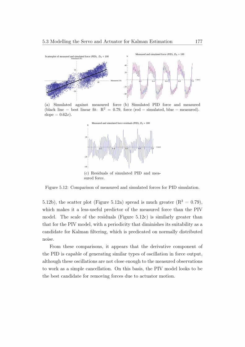
5.3 Modelling the Servo and Actuator for Kalman Estimation 177
åååå
åå
åååååååå
åå
ååååååå
ååå
åååååå
åå
åå
åååååå
åå
åå å åååå
ååå
åååååå
åååå å å å ååå
åååååååå åååå
åå
åå
åå
ååå
åå
å
åå
åååå
åå
å
ååå
å åååå
å
åå
åååååååååååå å
åååååå
ååååååååååå å å
åå
åååååå
åååååååååå å
åå
åå
å åååå
åååååååååå å å
å åå
ååååå
åå
å
åå
ååååå
åå
åååååååå
åå
ååå
ååååååå
åååååå
åå
åå
ååååå
ååååå
ååååå
åå
åååååå
åå
ååå
å å åå ååååå
åååååå
ååå
åå å å å å åååå
åå
åå
å
å
å
å
å
å
åååå
å
å
å
å
å
åå
ååå
å
å
å
å
ååååå
å
å
å
å
ååååå
å
å
å
å
åååååå
å
å
å
ååååååå
ååååååå
åå
å
å
åå
åå å åååå
ååååå
åå
å
å
å
åå
å å å ååååå
åååå
åå
å
åå
åååå
åå
å
ååå
ååååå
å
ååå
åååå
åå
åååååå
åå
åå
ååå
ååååå
ååååååå
åå
åå
ååååå
åå
åå
åå ååååå
åå
ååå åå
åå
åå
åå å å å
ååå
ååå
åå
åå
å
å
å
åååå
åå
å
å
å
ååååå
å
å
å
å
ååååå
åå
å
å
ååååå
ååå
ååååååå
åå
åå
åååååå
ååå
ååååååå
åå
åå å åå
åå
åå
ååååå
åååå
åå
å åå å
ååå
åå
å
åå
å
å
å
ååå å
å
å
å
å
å
åååå
åå
å
å
å
ååååå
å
å
å
ååååå
åå
åååå
åååååååå
ååååå
åå
åå
ååååå
ååååå
ååååå
åå
åå
åååå å
åååå
åå å å
åååå
åå
åå
å
å
å
ååååå
å
å
å
å
ååååå
å
å
å
å
åååå
åå
å
å
åå
åååååå
å
åå
åååååå
å
åå
åå å å
ååååå
åååååå
ååååå åå å
åå
ååå
ååååå
åååå
ååå å
åå
åå
å
å
å
å
å
åå
ååå
å
å
å
å
åå
å åå
å
å
å
å
åå
åååå
å
å
å
ååååå
å
å
å
å
åå
åååå
å
å
å
åå
ååååå
ååååå
ååå
åå
ååå
ååååå
åå
åå
ååååå
å
å
å
åå
åå
å
å
åå
å
å
å
å
åå
ååå
å
å
å
å
åååå
åå
å
å
å
åååååå
å
å
å
ååååååå
å
å
åå
ååååå
å
å
åå
ååååååååå
å å åå
åå
åå
ååååå
ååååååå å å
åå
å
å
ååå
åå
åå
åå
å
åå
åååååå
åååå
ååååå
åå
ååååååå
åååååååååå
ååå
ååååååå
åååååååååå
ååååååå
åå
åå
åååååå
åå
ååååååå
åå
å
åå
å
åå
åå
å
åå
åååååå
åå
ååå
ååååå
åå
åå
ååååååååå
åå å åååååå
ååååååååååå
å å å ååååååååå
åå
åååå
åå å åå
ååååååå
åå
åå
å
å
å
å
å
å
å
å
å
å
ååååå
å
å
å
å
åååååå
å
å
å
ååååå
å
å
å
åååååå
åå
åå
åå ååå
åå
åå
åå
åååå
ååå
åå åå å
ååååå
åååå å
ååå
åååå å å
ååå
å
å
åå
å
å
å
å
å
åååå
å
å
å
å
å
åååå
å
å
å
å
å
ååååå
å
å
å
å
åå
åååå
å
å
åå
ååååå
å
å
å
åå
å å åååå
åå
åååååå
å
åååå å å
åå
ååååååå
ååå
å
åå
å
å
å
å
å
å
å
ååååå
å
å
å
å
ååååå
å
å
å
å
ååååå
å
å
å
å
åååå
åå
å
ååå
å åååå
å
å
åå
åååå
åå
ååå
å å å åå
åååå
åååå
ååå
åååååå
åå
å
åå
å
å
å
å
å
å
ååååå
å
å
å
å
åå
ååå
å
å
å
å
åååååå
å
å
å
åå
å ååå
å
å
åå
ååååå
å
å
å
ååå å å
åå
ååååååå
ååå
åååååå å
åå
å ååååå
åå
åå
åå
å
å
å
å
å
åååå
åå
å
å
å
åå
åååå
å
å
å
ååååå
å
å
å
å
åå
åååååå
åå
ååååå
åå
ååå
åååååå
åååååå
åå
åååååååå
ååååå åå
åå
å
åå
å
å
å
åå
åå
åååå
ååå
åååååååååååååå
åå
ååååååååå
åå
ååååå
åå
åååååååååå
åå å å å åå å
åå
åå
ååååå
ååå åå
åå
å
å
åå
å
å
å
å
å
å
åååå
å
å
å
å
å
åååååå
å
å
å
åååå
åå
å
å
åååååå
åå
åå
åååå
åå
åå
ååå
å å å åå
ååå
åååååå
åå
åå
åå åå å åååå
åå
åå
åå
å
å
å
å
åå
ååå åå
åå
åååååå
ååååååååå
åå
ååååå
ååååååååååå
åå
åå
ååååååå
ååååååå
åå
åå
åå
å å åååååå
åå
åå
å
å
å
å
å
å
å
å
ååå
å
å
å
å
å
å
åååå
å
å
å
å
å
åååå
å
å
å
å
å
åååå
å
å
å
å
åååå å
å
å
å
å
åå
åååå
ååå
åå
åå åå
å
å
å
ååååå
ååå ååååå
å
åå
å
å
å
å
å
å
ååå
å
å
å
å
å
åååå
åå
å
å
å
ååååå
å
å
å
å
ååååååå
ååå
ååååå
å
å
ååå
ååååå
åå
åå å åå
åå
åå
åå
å å ååååå
åå
åå
å
å
å
å
å
å
å
åååå
åå
å
å
åå
åå ååå
å
å
åå
åååå
å
å
å
åå
ååååå
ååå
åååå
åå
ååå
åååååå
åå
åååååå
åå
åå
åååååååå
åå
å
ååå
å
å
å
å
å
åååå
å
å
å
å
å
åå åå
å
å
å
å
å
åååå
åå
å
å
ååååå å
åååååååå
ååå
å
ååååå å
åå
åå
åå ååå
ååå
ååå
å åå å å åå
åå
åå
å
å
å
å
å
å
ååå
å
å
å
å
å
å
åååå
å
å
å
å
å
ååå
å
å
å
å
å
å
åå åå
å
å
å
å
åå
åååå
å
å
å
åååå å
ååå
åå
åååå
åå
å
å
åå
åå å å åå
åå
åå
å
å
å
å
å
å
ååå
åå
å
å
å
ååååå
å
å
å
å
åååååå
å
å
å
åå
ååååååå
ååååååå
å
å
åå
å å å ååå
åå
ååååå
åå
åååå å å å å
å åååå
å
å
å
å
å
å
åååå
åå
å
å
ååååååå
å
å
ååååå
ååå
å
ååå åååå
ååå
ååååååå
ååååå å åå
åå
ååå
åååååå
åå
åå å åå
ååå
å
å
å
å
å
å
å
å
åååå
å
å
å
å
ååååå
å
å
å
å
åååååå
å
å
å
åå
å åååå
å
åå
åååååå
å
å
åå
å å å åå
åå
ååååå
åå
å
åå
åå å å
åå å
å
å
å
å
å
å
å
å
ååå
å
å
å
å
å
å
åååå
å
å
å
å
å
åååå
å
å
å
å
å
åååå
åå
å
å
åå
åååå
å
å
å
å
åååå å
ååå
åå
åååå
å
å
å
åååååå
åå
å
åå
åå
å
å
å
åååå
å
å
å
å
å
åååå
åå
å
å
ååååå
åå
å
å
åååå
ååå
ååååååå
ååå
ååååååå å
åå
åå
å åååå
ååå
åå å å
å å
å
åå
å
å
å
å
å
å
ååå
å
å
å
å
å
å
ååååå
å
å
å
å
åååå
å
å
å
å
å
åååå
åå
å
å
ååååå
åå
å
å
å
åå
åååå
åå
åå
ååååå
å
å
å
åå
åå
ååå
å
å
å
å
å
å
å
åååå
å
å
å
å
å
åååå
å
å
å
å
åååååå
å
å
å
å
åååååå
å
åå
å å åå
å
å
å
å
åå
åååååå
ååå
å å åå
åå
å
åååå
åå
å
å
å
å
å
å
å
å
åååå
å
å
å
å
å
åååå
å
å
å
å
åååå
åå
å
å
å
åå
åååå
åå
åå
ååååå
å
å
å
åååååå
åå
åååååå
åå
åå
åå
ååå
å
å
å
å
å
å
å
å
å
åååå
å
å
å
å
åååå
å
å
å
å
å
åååååå
å
å
å
ååååååå
å
ååååå
åå
å
å
å
åå
å åååååå
ååå å å
åå
å
åå
åå
åå
åå
å
å
å
å
å
å
ååå
å
å
å
å
å
å
ååå
å
å
å
å
å
å
åååå
å
å
å
å
å
ååå å
åå
å
å
åå
åååå
å
å
å
å
åå
å ååå
åå
ååååå
åå
å
å
ååå
ååå
å
å
å
å
å
å
å
ååå
å
å
å
å
å
åååååå
å
å
å
åå
ååå
å
å
å
å
åååååå
åå
åå
å ååååå
å
å
ååååå å
åå
åå
åå å å å
åååå
åå
å
å
å
å
å
å
å
å
åå
åååå
å
å
åå
åååååå
åå
ååååå
åå
åå
åå
ååååå
åå
åååååå
ååååå
åååååå
ååååååå
åå
åå
åå
åå
å
å
å
å
å
å
å
ååå
å
å
å
å
å
å
ååå
å
å
å
å
å
å
åååå
å
å
å
å
å
åååå
å
å
å
å
åååå
åå
å
å
å
å
åå å å å
åå
å
åå
åå åå
å
å
å
å
å
å
å
å
å
å
å
å
å
åååå
å
å
å
å
å
ååååå
å
å
å
å
åååå
å
å
å
å
å
åå
ååå
åå
å
ååååå
åå
å
å
å
ååååå
åå
åå
åå ååå
åå
å
å
åå
å
å
å
å
å
å
å
å
åå å
å
å
å
å
å
å
ååå
å
å
å
å
å
å
ååå
å
å
å
å
å
å
åååå
åå
å
å
ååååå
å
å
å
å
å
ååååå
ååå
åå
å å åå
å
å
å
å
å
å
å
å
å
å
å
å
å
ååå
å
å
å
å
å
å
ååå
åå
å
å
å
å
ååååå
å
å
å
å
åååå
åå
å
åå
åååå
åå
å
å
å
åå
å å åå
åååå
åååååå
å
å
å
å
å
å
å
å
å
å
å
ååå
å
å
å
å
å
å
ååå
å
å
å
å
å
å
åååå
å
å
å
å
å
åååå
å
å
å
å
åå
å åå
å
å
å
å
å
åå
å åå
åå
å
å
åå
å åå
å
å
å
å
å
å
å
å
å
å
å
å
å
ååå
å
å
å
å
å
ååååå
å
å
å
å
åååå
å
å
å
å
å
åååå
åå
å
å
ååååå
å
å
å
å
å
åå
å åååå
å
å
ååå
åå
å
åå
å
å
å
å
å
å
å
å
åååå
å
å
å
å
å
åååå
å
å
å
å
å
ååååå
å
å
å
å
åååååå
å
å
åå
å ååå
å
å
å
å
åå
å å åå
åå
åå
åå å å
åå
å
å
å
å
å
å
å
å
å
å
åååå
å
å
å
å
å
ååå
å
å
å
å
å
å
ååå
å
å
å
å
å
å
åååå
å
å
å
å
åååå
åå
å
å
å
å
ååååå
å
å
å
åååååå
å
å
å
å
å
å
å
å
å
å
ååå
å
å
å
å
å
å
åååå
å
å
å
å
å
åååå
å
å
å
å
å
åååååå
å
å
åå
å å åå
å
å
å
å
åå
å å åå
å
å
åå å å å å
å
å
å
å
å
å
å
å
å
å
å
åååå
å
å
å
å
å
åååå
å
å
å
å
å
ååå
å
å
å
å
å
å
åååå
å
å
å
å
åååå
åå
å
å
å
å
åååå
åå
åå
ååå
åå
åå
å
å
å
å
å
å
å
å
ååå
å
å
å
å
å
å
åååå
å
å
å
å
å
åååå
å
å
å
å
å
åååå
åå
å
å
åå
å åå
å
å
å
å
å
åå
åå åå
å
åå
å å å åå
å
å
å
å
å
å
å
å
å
å
ååå
å
å
å
å
å
åååå
å
å
å
å
å
åååå
å
å
å
å
å
åååå
åå
å
å
åå
åååå
å
å
å
å
åå
å å åå
å
ååååå
åå
å
å
å
å
å
å
å
å
å
åå å
å
å
å
å
å
å
ååå
å
å
å
å
å
å
ååå
å
å
å
å
å
å
åååå
åå
å
å
åååå
åå
å
å
å
å
åå
å ååå
åå
å ååå
åå
å
å
å
å
å
å
å
å
åååå
å
å
å
å
å
åååååå
å
å
ååååå
åå
å
å
å
åå
åååååå
ååååå
åå
å
å
ååå
ååååå
åå
å å åååå
å
å
å
å
å
å
å
å
ååå
å
å
å
å
å
å
ååå
å
å
å
å
å
å
åååå
å
å
å
å
å
åå å å
åå
å
åå
åå ååå
å
å
å
å
åå
å å åå
ååååå
å
å
å
å
å
å
å
å
å
å
åååå
å
å
å
å
å
ååååå
å
å
å
åååå å
å
å
å
å
å
åå
åååå
åå
ååååå
åå
å
å
åå
ååååå
åå
åååå
å
å
å
å
å
å
å
å
å
åååå
å
å
å
å
å
åååååå
å
å
åååååå
å
å
å
å
åååååå
åå
åå
å å åååå
å
åå
åå å å å
åå å å å
åå
å
å
å
å
å
å
å
å
åååå
å
å
å
å
å
ååååå
å
å
å
å
ååååå
å
å
å
å
åååååå
åå
åå
åååå
å
å
å
å
åå
å å ååååååå
å
å
å
å
å
å
å
å
å
å
ååå
å
å
å
å
å
åå
åååå
å
å
å
ååååå
å
å
å
å
åååååå
åå
ååååå
åå
å
å
å
åå
å åå åå
åå å åå
å
å
å
å
å
å
å
å
å
åååå
å
å
å
å
å
åååå
å
å
å
å
å
åååå
å
å
å
å
å
ååååå
åå
åååå åå
åå
å
å
å
åå
åååå
åååååå
å
å
å
å
å
å
å
å
ååå
å
å
å
å
å
å
åååå
å
å
å
å
å
ååå
åå
å
å
å
å
åååå
åå
åå
ååååå
å
å
å
å
å
åå
å å åå
å å åå
åå
å
å
å
å
å
å
å
åååå
å
å
å
å
å
ååååå
å
å
å
å
ååååå
å
å
å
å
åå
åååå
åå
ååååå
åå
å
å
å
ååå å å
ååååå
åå
å
å
å
å
å
å
å
å
ååå
å
å
å
å
å
å
åååå
å
å
å
å
ååååå
å
å
å
å
å
åååå
åå
å
åå
åååå
å
å
å
å
åå
å ååå
ååååå
å
å
å
å
å
å
å
å
ååå
å
å
å
å
å
å
ååååå
å
å
å
åå
åååå
å
å
å
å
åååå
ååå
åå
åååå
å
å
å
å
å
åå
åååå
ååååå
å
å
å
å
å
å
å
åå
ååå
å
å
å
å
ååååå
å
å
å
ååååå
åå
å
å
å
åååååå
ååå
å å å åå
åå
å
åå
åå å å å
åå ååå
å
å
å
å
å
å
å
å
ååå
å
å
å
å
å
å
åååå
å
å
å
å
å
ååå
å
å
å
å
å
å
åååå
åå
å
å
åååå
åå
å
å
å
å
åå
ååå
åå å å
åå
å
å
å
å
å
å
åååå
å
å
å
å
å
åååå
å
å
å
å
å
åååå
å
å
å
å
å
åååå å
åå
åååååå
åå
å
å
å
åå
å å åå
å åå
å
å
å
å
å
å
å
å
å
ååå
å
å
å
å
å
åååååå
å
å
å
ååååå
å
å
å
å
å
ååååå
åå
åå
åååå
å
å
å
å
åå
å å åå åååå
åå
å
å
å
å
å
å
ååå
å
å
å
å
å
å
åååå
å
å
å
å
å
åååå
å
å
å
å
å
åå
å åååå
ååå åå
åå
å
å
å
å
åå
å å å å ååå
åå
å
å
å
å
å
å
åååå
å
å
å
å
å
ååå
åå
å
å
å
åååå
å
å
å
å
å
å
åååå
åå
åååååå
åå
å
å
å
åå
åååå
ååå
å
å
å
å
å
å
å
å
åååå
å
å
å
å
å
åååå
å
å
å
å
åååå
åå
å
å
å
å
ååååå
åå
åå
åååå
å
å
å
å
å
åå
å å ååååå
å
å
å
å
å
å
å
å
ååå
å
å
å
å
å
åååå
å
å
å
å
å
åååå
å
å
å
å
å
å
åååå
åå
åå
åååå
å
å
å
å
å
åå
åååååå
åå
å
å
å
å
å
å
ååå
å
å
å
å
å
å
åååå
å
å
å
å
å
ååå
å
å
å
å
å
å
åå
ååå
å
å
å
åååå
åå
å
å
å
å
åå
ååååå å
åå
å
å
å
å
å
å
åååå
å
å
å
å
å
ååååå
å
å
å
åååå
åå
å
å
å
å
åå
ååååå
åå
åååå
å
å
å
å
å
åååå
ååååå
å
å
å
å
å
å
ååå
å
å
å
å
å
å
ååååå
å
å
å
å
åå å
åå
å
å
å
å
åå
åå åå
ååå
å å å åå
å
å
å
å
ååååå å
å åå
å
å
å
å
å
å
ååååå
å
å
å
å
åååååå
å
å
ååå åå
å
å
å
å
å
åå
ååååå
åå
åååååå
å
å
åå
åååå
åååå
å
å
å
å
å
å
åååå
å
å
å
å
å
ååååå
å
å
å
ååå å
åå
å
å
å
å
åå
åå åå
åå
ååå å
åå
å
å
å
å
ååååå å å
å
å
å
å
å
å
å
å
ååå
å
å
å
å
å
åååå
å
å
å
å
å
ååå
å
å
å
å
å
å
å
ååå
åå
å
åå
ååå
åå
å
å
å
å
åå
åååååå
å
å
å
å
å
å
å
ååå
å
å
å
å
å
å
åååå
å
å
å
å
ååå
å
å
å
å
å
å
å
ååååå
å
å
åå
åååå
å
å
å
å
å
åå ååååå
å
å
å
å
å
å
å
åååå
å
å
å
å
åååå
å
å
å
å
å
ååååå
å
å
å
å
å
åååå
åå
åå
ååååå
å
å
å
å
åå
ååååå
å
å
å
å
å
å
å
åååå
å
å
å
å
å
åååå
å
å
å
å
å
åååå
å
å
å
å
å
å
ååå
ååå
åå
å ååå
å
å
å
å
å
åå
åå ååå
å
å
å
å
å
å
å
ååå
å
å
å
å
å
å
ååå
å
å
å
å
å
åååå
å
å
å
å
å
å
åååå
å
å
å
åå
åååå
å
å
å
å
å
ååååå
åå
å
å
å
å
å
åååå
å
å
å
å
å
åååå
å
å
å
å
åååååå
å
å
å
å
åå
å å ååå
åå
åå ååå
å
å
å
å
åå
å å åå
å
å
å
å
å
å
å
å
åååå
å
å
å
å
ååååå
å
å
å
å
åååå
å
å
å
å
å
å
åååååå
åå
ååååå
å
å
å
å
åå
åå å åå
å
å
å
å
å
å
å
ååå
å
å
å
å
å
åååå
å
å
å
å
å
ååå
å
å
å
å
å
å
å
åå å å
åå
åå
åå å
åå
å
å
å
å
åå
åå å
å
å
å
å
å
å
å
ååå
åå
å
å
å
å
åååå
å
å
å
å
ååååå
å
å
å
å
å
åå
åååå
åå
åååå
åå
å
å
å
åå
ååååå
å
å
å
å
å
å
å
ååå
å
å
å
å
å
åååå
å
å
å
å
å
ååå
å
å
å
å
å
å
å
åå åå
å
å
å
åå
å åå
å
å
å
å
å
åå
ååå
å
å
å
å
å
å
å
ååå
å
å
å
å
å
å
åååå
å
å
å
å
åååå
å
å
å
å
å
å
åååå
åå
åå
åååå
åå
å
å
å
åå
åååå
å
å
å
å
å
å
å
åååå
å
å
å
å
å
ååå
å
å
å
å
å
ååååå
å
å
å
å
å
ååååååå
ååå å å
åå
å
å
å
å
åå å
ååå
å
å
å
å
å
åååå
å
å
å
å
å
ååå
å
å
å
å
å
åååå
å
å
å
å
å
å
åååå
åå
åå
åååå
åå
å
å
å
å
åå å å å
å
å
å
å
å
å
å
ååå
å
å
å
å
å
åååå
å
å
å
å
å
ååå
å
å
å
å
å
å
å
åå å å
åå
åå
ååååå
å
å
å
å
åå
å åå
å
å
å
å
å
å
ååå
å
å
å
å
å
å
ååå
å
å
å
å
å
åååå
å
å
å
å
å
å
åå
ååååååååååå
å
å
å
å
å
ååå
åå
å
å
å
å
å
å
ååå
åå
å
å
å
åååååå
å
å
ååå åå
åå
å
å
å
å
ååå å å å
åå
åå å åå
åå
å
åå
åå
ååå
å
å
å
å
å
å
ååå
å
å
å
å
å
å
ååå
å
å
å
å
å
åååå
å
å
å
å
å
å
åååå
åå
å
åå
åååå
å
å
å
å
å
ååå
å
å
å
å
å
å
å
ååå
å
å
å
å
å
ååååå
å
å
å
å
ååå
å
å
å
å
å
å
å
åå å å
åå
åå
ååå åå
å
å
å
å
åå
å
åå
å
å
å
å
å
å
ååå
åå
å
å
å
åå
ååååå
ååå
åååå
å
å
å
å
å
åå
åååååååååå
åå
åå
åå
åå
åå
å
å
å
å
å
å
ååå
å
å
å
å
å
å
åååå
å
å
å
å
åå å
å
å
å
å
å
å
å
åå å å
åå
å
åå
å å åå
å
å
å
å
å
åå
å
å
å
å
å
å
å
ååå
å
å
å
å
å
åå
ååå
å
å
å
å
åååå
å
å
å
å
å
å
åååå
åå
åå
ååååå
å
å
å
å
ååå
åå
å
å
å
å
å
å
ååå
å
å
å
å
å
ååååååå
å
åå
åååå
å
å
å
å
å
åå
å å åå
åå
å åååå
åå
å
åå
åå
å
å
å
å
å
å
å
ååå
å
å
å
å
å
å
ååå
å
å
å
å
å
åååå
å
å
å
å
å
å
åå
ååå
åå
ååååå
åå
å
å
å
å
å
åå
å
å
å
å
å
å
ååå
å
å
å
å
å
å
åååå
å
å
å
å
åååå
å
å
å
å
å
å
åååå å
åå
åå å å å
åå
å
å
å
ååå
å
å
å
å
å
å
å
åååå
å
å
å
å
å
ååå
å
å
å
å
å
åååå
å
å
å
å
å
-40 -20 20 40Measured HNL
-50
50
Simulated HNLScatterplot of measured and simulated force HPIDL, DN = 100
(a) Simulated against measured force(black line = best linear fit: R2 = 0.79,slope = 0.62x).
6.2 6.4 6.6 6.8 7.0t HsecL
-40
-20
20
40
NMeasured and simulated force HPIDL, DN = 100
(b) Simulated PID force and measuredforce (red = simulated, blue = measured).
6.2 6.4 6.6 6.8 7.0t HsecL
-40
-20
20
NMeasured and simulated force residuals HPIDL, Dn = 100
(c) Residuals of simulated PID and mea-sured force.
Figure 5.12: Comparison of measured and simulated forces for PID simulation.
5.12b), the scatter plot (Figure 5.12a) spread is much greater (R2 = 0.79),which makes it a less-useful predictor of the measured force than the PIVmodel. The scale of the residuals (Figure 5.12c) is similarly greater thanthat for the PIV model, with a periodicity that diminishes its suitability as acandidate for Kalman filtering, which is predicated on normally distributednoise.
From these comparisons, it appears that the derivative component ofthe PID is capable of generating similar types of oscillation in force output,although these oscillations are not close enough to the measured observationsto work as a simple cancellation. On this basis, the PIV model looks to bethe best candidate for removing forces due to actuator motion.

5.3 Modelling the Servo and Actuator for Kalman Estimation 178
Response to Constant Position Command
Until this point we have been simulating the closed-loop behaviour of thesystem — that is, the force output based on actuator motion are part of thesame computational system with no external inputs. Measured data was onlyused for comparison in parameter estimation, not as an input to the system.However, the filtering system will have actuator position as an input, andwill have the ability to determine the position error the servo was acting on.The sampling and timing diagram, Figure 5.6 in §5.3.1, shows how this iscoordinated.
2 4 6 8 10 12 14t HsecL
-0.08
-0.06
-0.04
-0.02
0.02
error HmmLActuator stroke position error
(a) Position error.
2 4 6 8 10 12 14t HsecL
-10
10
20
force HNLServo force output
(b) Servo force output.
1.0 1.1 1.2 1.3 1.4 1.5t HsecL
-0.08
-0.06
-0.04
-0.02
error HmmLActuator stroke position error
(c) Zoomed position error.
1.0 1.1 1.2 1.3 1.4 1.5t HsecL
-15
-10
-5
5
force HNLServo force output
(d) Zoomed force output.
Figure 5.13: Actuator and servo response to constant position command withdisturbance.
Data collected in a separate test is used to assess and calibrate a model forKalman filtering. In this step, we are looking to tune a model that respondswith an appropriate magnitude to an externally applied force, but minimisesthe oscillations due to noisy measurements and process components.

5.3 Modelling the Servo and Actuator for Kalman Estimation 179
The servo was commanded to hold a constant position midway throughits stroke length. It was laid on its side, then rotated 90 degrees such that theproduct of stroke mass and gravity was acting as a constant force (roughly5N) on the stroke. This force caused a change in actuator position, andthe servo acted to remove the position error. Stroke position and the forceoutput from the servo was recorded; these noisy signals are shown in Figures5.13a and 5.13b, respectively, along with zoomed segments for comparisonwith simulations.
The PID and PIV models are simulated in an open loop, using only themeasured position error shown in Figure 5.13a as an input; results of thesesimulations are shown in Figure 5.14.
2 4 6 8 10 12 14t HsecL
-15
-10
-5
5
10
15
20
NSimulated force HPIDL
(a) PID model force output.
2 4 6 8 10 12 14t HsecL
-8
-6
-4
-2
2
4
NSimulated force HPIVL
(b) PIV model force output.
1.0 1.1 1.2 1.3 1.4 1.5t HsecL
-15
-10
-5
5
NSimulated force HPIDL
(c) Zoomed PID model force output.
1.0 1.1 1.2 1.3 1.4 1.5t HsecL
-6
-5
-4
-3
-2
-1
1N
Simulated force HPIVL
(d) Zoomed PIV model force output.
Figure 5.14: PID and PIV servo model simulations.
The PID model is the best match for the noisiness of the measured signal,however, we are looking to minimise noise in the simulation; the PIV is animprovement, with the shape of the force response easily made out. As in thechirp simulations, an analysis of force due the separate components shows the
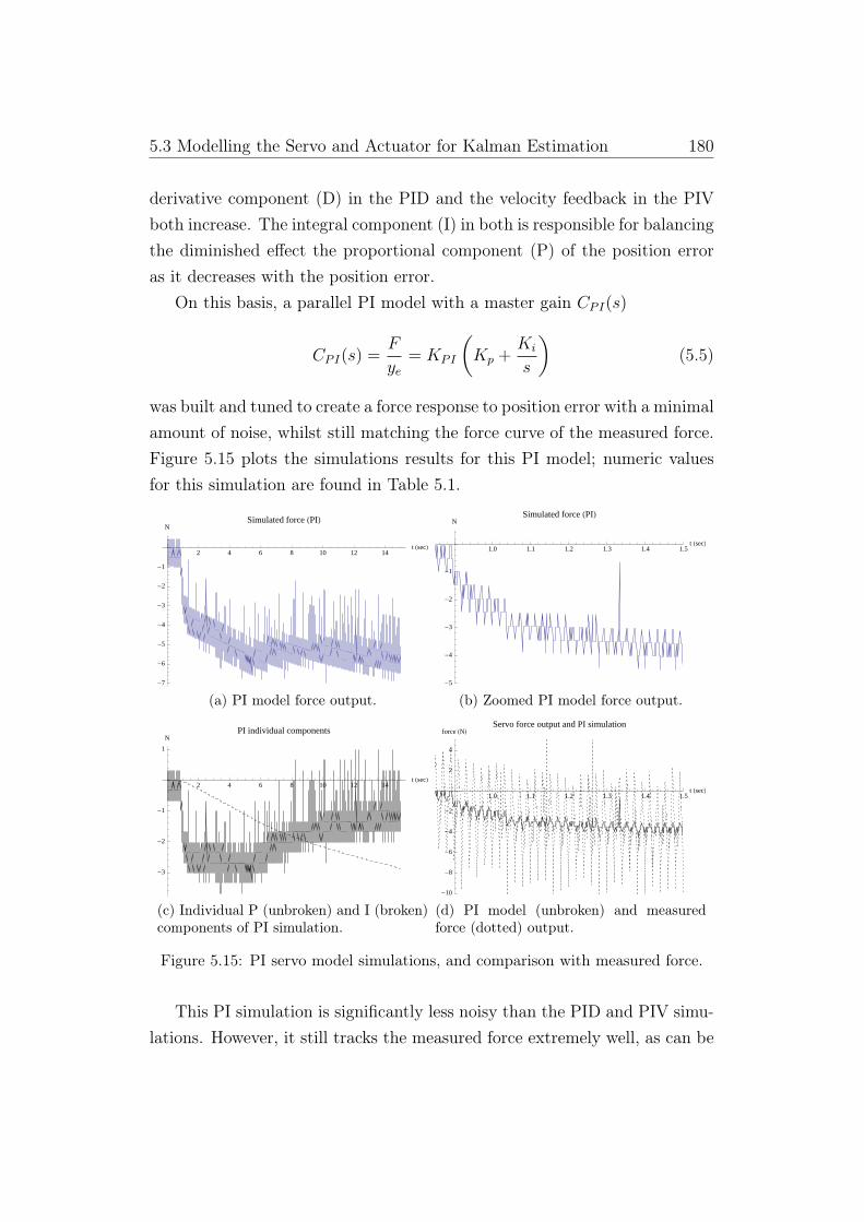
5.3 Modelling the Servo and Actuator for Kalman Estimation 180
derivative component (D) in the PID and the velocity feedback in the PIVboth increase. The integral component (I) in both is responsible for balancingthe diminished effect the proportional component (P) of the position erroras it decreases with the position error.
On this basis, a parallel PI model with a master gain CPI(s)
CPI(s) =F
ye= KPI
(Kp +
Ki
s
)(5.5)
was built and tuned to create a force response to position error with a minimalamount of noise, whilst still matching the force curve of the measured force.Figure 5.15 plots the simulations results for this PI model; numeric valuesfor this simulation are found in Table 5.1.
2 4 6 8 10 12 14t HsecL
-7
-6
-5
-4
-3
-2
-1
NSimulated force HPIL
(a) PI model force output.
1.0 1.1 1.2 1.3 1.4 1.5t HsecL
-5
-4
-3
-2
-1
NSimulated force HPIL
(b) Zoomed PI model force output.
2 4 6 8 10 12 14t HsecL
-3
-2
-1
1
NPI individual components
(c) Individual P (unbroken) and I (broken)components of PI simulation.
1.0 1.1 1.2 1.3 1.4 1.5t HsecL
-10
-8
-6
-4
-2
2
4
force HNLServo force output and PI simulation
(d) PI model (unbroken) and measuredforce (dotted) output.
Figure 5.15: PI servo model simulations, and comparison with measured force.
This PI simulation is significantly less noisy than the PID and PIV simu-lations. However, it still tracks the measured force extremely well, as can be

5.3 Modelling the Servo and Actuator for Kalman Estimation 181
seen in Figure 5.15d. A comparison of the error input signal in Figure 5.13aand the zoomed portion of the PI simulation shown in Figure 5.15b showshow the proportional component dominates the signal. As mentioned earlier,the integral component tracks long term error and keeps the force signal atapproximately -5 N despite the decrease in position error; this is illustratedin Figure 5.15c.
Re-tuned PIV Model for Kalman Estimation, PIVK
2 4 6 8 10 12 14t HsecL
-5
-4
-3
-2
-1
NSimulated force HPIV Kv=25, Vn=500L
(a) Re-tuned PIV model force output.
1.0 1.1 1.2 1.3 1.4 1.5t HsecL
-4
-3
-2
-1
NSimulated force HPIV Kv=25, Vn=500L
(b) Zoomed re-tuned PIV model force out-put.
1.0 1.1 1.2 1.3 1.4 1.5t HsecL
-10
-8
-6
-4
-2
2
4
force HNLServo force output and PIV HKv=25, Vn=500L simulation
(c) Re-tuned PIV model (unbroken) andmeasured force (dotted) output.
1.0 1.1 1.2 1.3 1.4 1.5t HsecL
-5
-4
-3
-2
-1
force HNLPI and PIV HKv=25, Vn=500L simulations
(d) Re-tuned PIV model (unbroken) and PImodel (dotted) output.
Figure 5.16: Re-tuned PIV servo model simulations, comparison with measuredforce, and comparison with PI model.
Although the noise associated with velocity and derivative feedback isabsent in the position model, there is another form of noise introduced by thedominance of the proportional component: the sudden jumps proportional tothe smallest quantum of the position sensor. Re-instituting velocity feedback

5.4 Building the Kalman Estimators 182
at a lower gain can smooth the sudden jumps in due to the proportionalcomponent of the PIV.
The velocity feedback gain estimated during the system identificationprocess, Kv is quite high and played an important role in reproducing thehigh-frequency chirp signal. This reproduction is no longer our goal. Re-simulating the PIV model with lower Kv gain and higher filter pole returns asignal of similar noise magnitude to the PI model, but much with smoothedjumps. In this re-tuned PIV model, Kv = 25, and Vn = 500.
The plots in Figure 5.16 shows the improvement this adjustment makes;the re-tuned PIV model still tracks the measured force very well (Figure5.16c), and is smoother than the PI model (Figure 5.16d). This re-tunedPIV model will now form the basis of a Kalman estimator for filtering themeasured force signal; it will be referred to as PIVK.
5.4 Building the Kalman Estimators
As well as the Kalman estimator based on the developed PIVK servo model,two other Kalman estimators will be built in this section: a position errorestimator, and an estimated force estimator. Four filtering configurations,illustrated in Figure 5.17, will then be demonstrated:
1. No filter, CPIVK response to position error only;
2. Filtered with unfiltered position data as input;
3. Filtered with filtered position data as input; and
4. Filtered with filtered position data as input, then filtered again.
The unfiltered model is included to demonstrate the Kalman estimator’sability to reconcile noisy measurements and imperfectly modelled systems;in particular, the position error signal contains significant drift due to theintegral component of the servo, and the constant force of the actuator strokeand gravity. The servo model is reasonably accurate, but also exhibits drift.

5.4 Building the Kalman Estimators 183
Figure 5.17: Force signal filtering schemes. Scheme 4 provides the most sensitiveand clean estimation of servo output force, and, therefore, user-applied force.
The Kalman estimated models (2–4) eliminate this drift by also taking intoaccount noisy measurements, which the open-loop servo model does not.
Filtering the position error allows more aggressive settings for noise co-variance in the servo model estimator. Aggressive in this context meansputting more trust in the noisy measurements than they deserve in orderto catch sudden changes. An trustworthy process model with clean inputwill minimise process noise to leave a reasonably clean but accurate forceestimate. This estimate is then filtered again, returning a force sensor signaleasily incorporated into the control system.
5.4.1 The Kalman Estimator — Technical
The Kalman estimator is a recursive algorithm that estimates the state ofan n state linear dynamic system x which is perturbed by process noise wkand can be described by a linear stochastic difference equation
xk = Axk−1 + Buk−1 + wk−1 (5.6)

5.4 Building the Kalman Estimators 184
whereA is an n×n state transition matrix relating the state x at the previoustime step k− 1 to the current time k, absent any other inputs, B is an n× lmatrix relating l control inputs to the state xk, and the system is perturbedby process noise wk.
The system is observed with m noisy measurements zk
zk = Hxk + Duk + vk (5.7)
where H is an m × n matrix linearly relating the state to the measurementzk, D is a input-feedthrough gain matrix, and vk is measurement noise. Bothwk and vk are assumed to be independent zero-mean Gaussian processes withnormal probability distribution and covariances Q (process) and R (measure-ment):
p(w) = N(0, Q)
p(v) = N(0, R) (5.8)
Welch and Bishop [130] provide an excellent explanation of the Kalmanestimator, and Grewahl and Andrews [58] provide the mathematical andhistorical background.
The Kalman Algorithm
The two-step recursive algorithm’s goal is to minimise the covariance Pk ofthe error between the system’s state xk and the estimated state xk
ek = xk − xk
Pk = E[eke
Tk
](5.9)
In the prediction step, an a priori state estimate x−
k is made based onthe state estimate from the previous time step xk−1 and known control inputuk−1. An a priori error covariance value P
− is also calculated based onits value at the previous time step, propagated through the state transition

5.4 Building the Kalman Estimators 185
matrix A and summed with the user-specified process covariance Q.
x−
k = Axk−1 + Buk−1
P−
k = APk−1AT +Q (5.10)
The first operation in the update step is finding an updated Kalmangain. Kk is calculated from the measurement matrix H, the a priori errorcovariance P
−
k , and the user-specified measurement noise covariance R:
Kk =P
−
kHT
HP−kH
T +R(5.11)
The next operation returns a new state estimate xk determined by acombination of the a priori state estimate and the difference between a mea-surement prediction based on this state and a noisy measurement of thesystem, or residual, weighted by the Kalman gain:
x = x−
k + Kk(zk −Hxk −Duk) (5.12)
The final operation in the update step is calculating a new error covariancevalue for use in the predict step of the next iteration of the algorithm.
Pk = P−k(In −HKk) (5.13)
Influence of Process and Measurement Noise Covariance
Aside from the quality of the model, the Kalman estimator has two designinputs that influence its performance: the process and measurement noisecovariance values, Q and R. They interact in the calculation of the Kalmangain, where along with the previous error covariance they determine theweighting of the residuals in the current time step, as seen in the update stepEq. (5.12).
If the Kalman gain is very small, the noisy measurement is disregardedand the state estimate is trusted. If the Kalman gain is very high, theestimate is ignored and the measurement is trusted. Looking at Eq. (5.11)

5.4 Building the Kalman Estimators 186
we see that as error covariance approaches zero, so does the Kalman gain,weighing the residual less heavily:
limP
−k → 0
Kk = 0
Looking back to the update stage Eq. (5.10), it is apparent how the valuefor Q determines the extent to which the estimate can be fully trusted, bysetting a lower limit for P , and, therefore, a limit on how much the stateestimate is trusted over the residual.
As the measurement noise covariance R approaches zero, the gain weighsthe residual more heavily. Again, looking at Eq. (5.11), we see that:
limR→ 0
Kk =1
H
These relationships are exploited for fine-tuning the responsiveness offorce sensing later in this chapter.
5.4.2 Kalman Estimator for Servo Model
A discrete-time Kalman estimator requires that the servo model PIVK beconverted into state-space form and discretised. State-space represents asystem with a state update equation, and a measurement equation. ThePIVK model has two inputs and two states, and the continuous-time state-space representation is:
x(t) = Ax(t) + Bu(t)
y(t) = Cx(t) + Du(t) (5.14)
where
A =
[0 0
0 −Vn
]; B =
[1 0
0 1
]; C =
[Ki KvV
2n
];D =
[Kp −KvVn
](5.15)
5.4 Building the Kalman Estimators 187
with two states x1, and x2 = x1, and two inputs ye and yo
x =
[x1
x2
]; u =
[ye
yo
]
This is discretised for a sampling-period of T by changing A and B to
A =
[1 0
0 (1− TVn)
]; B =
[T 0
0 T
]
The full model for the discretised system for Kalman estimation, includingprocess noise wk and measurement noise vk is
xk = Axk−1 + Buk−1 + wk
zk = Hxk + Duk + vk (5.16)
where zk replaces yk to represent noisy measurements, and C is renamed H
as per Kalman notational convention [58].Because we are quite confident in this process model based on the work
in the previous chapter, process noise covariance Q can be set quite low andmeasured noise covariance R can still be set quite low in order to aggressivelyfollow sudden changes. Here, R is set well below the noise covariance shownin earlier force sample (Figure 5.4a):
Q = 5× 10⁻⁴; R = 5 (5.17)
5.4.3 Position Error Estimator
Unlike the model for the servo, the input to the actuator which causes aposition error is not fully known — i.e., only the output of the servo isknown, not any external driving forces. This problem is of a similar natureto filtering accelerometer data, where it has been shown that a process modelfor Kalman filtering based on a simplified mass-spring-damper model of theinternal mechanics of an accelerometer yielding good noise reduction [67].

5.4 Building the Kalman Estimators 188
Because actuator position error will be the result of an external drivingforce acting on the actuator stroke (like user-applied force), it seems reason-able to use a simple mass-damper actuator model for the Kalman processmodel. Taking only the linear components of the actuator model presentedin §5.3.1, Eq. (5.3) becomes
myo + Fvyo = 0 (5.18)
where Fv is coefficient of viscous friction. Discretising this model and con-verting it to state-space form for Kalman estimation of position error gives:
yek =
[1 T
0 (1− TFv/m)
]yek−1
+
[0
T
]uk−1 + wk−1
zek =[1/m 0
]yek + vk−1 (5.19)
After extensive trial and error, the position error estimator is initialisedwith
Qe = 15; Re = 10−7 (5.20)
which reflects significantly greater confidence in the measurement, eventhough it is noisy, but also some confidence in the process model.
5.4.4 Estimated Force Estimator
Because there is no control delay associated with the Kalman estimator,there is no reason not to include a final estimator, smoothing the output ofthe servo estimator, which itself takes a filtered position estimate. This finalestimator takes the same form as the position error filter on the basis thatthe estimated force signal will reflect the user-applied force to the actuatorstroke, and is a product of the position error due to this driving force.
However, the gain on the mass-damper model is increased from 1 to 150.This increased gain makes the process model more responsive to noisy input,permitting a more sensitive overlap between the role of process and mea-surement noise for this Kalman estimator. Increasing the gain requires only

5.4 Building the Kalman Estimators 189
a change to the measurement expression from Eq. (5.19), which gives thefollowing process model for smoothing the previously estimated force:
F k =
[1 T
0 (1− TFv/m)
]F k−1 +
[0
T
]uk−1 + wk−1
zF k=[150/m 0
]F k + vk−1 (5.21)
The inclusion of a high gain to this model is significant because it guar-antees that the estimator will be responsive to quick changes, however theinertia and damping characteristics of the actuator model still ensure somesmoothness. This is a useful solution to the problem of time-lag that re-sults from process models in Kalman estimators that are too smooth, andthen weighted too heavily; in such instances, the estimator is reluctant tofollow quick changes promptly. This is particularly the case in systems withno input, or where the driving force is unknown, as in this system, and theestimator relies only on noisy measurements [130].
This high-gain model effectively leaves the user with only one parameterto adjust the smoothness and responsiveness of the force sensor, the processnoise covariance Q. A low value for Q indicates that the process modelshould be trusted, smoothing the signal. A higher value for Q indicatesthat the process model is less trustworthy, and the estimator should be moreresponsive to noisy measurements. A suitably small value for R, such asbetween 10−4 and 10−6, can be set and forgotten, whilst Q can be adjustedto suit the application requirements.
In the following results, R = 5×10⁻³ is used, with Q adjusted for smooth-ness.
5.4.5 Filtering Results
The first four plots in Figure 5.18 show the full 15 second force filteringresults for the force signal original shown in §5.2, and reproduced against theresult for an unfiltered PIVK model in Figure 5.18a.
The unfiltered PIVK model performs quite poorly here, with the propor-
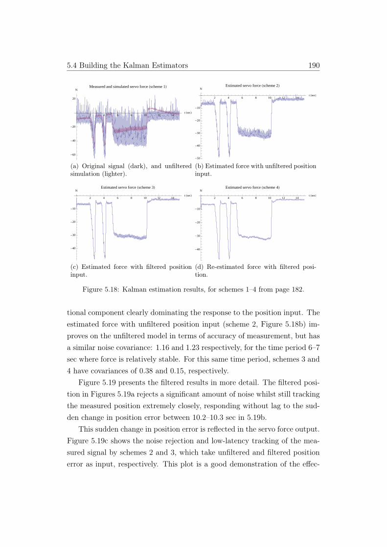
5.4 Building the Kalman Estimators 190
2 4 6 8 10 12 14t HsecL
-60
-40
-20
20
NMeasured and simulated servo force Hscheme 1L
(a) Original signal (dark), and unfilteredsimulation (lighter).
2 4 6 8 10 12 14t HsecL
-50
-40
-30
-20
-10
NEstimated servo force Hscheme 2L
(b) Estimated force with unfiltered positioninput.
2 4 6 8 10 12 14t HsecL
-40
-30
-20
-10
NEstimated servo force Hscheme 3L
(c) Estimated force with filtered positioninput.
2 4 6 8 10 12 14t HsecL
-40
-30
-20
-10
NEstimated servo force Hscheme 4L
(d) Re-estimated force with filtered posi-tion.
Figure 5.18: Kalman estimation results, for schemes 1–4 from page 182.
tional component clearly dominating the response to the position input. Theestimated force with unfiltered position input (scheme 2, Figure 5.18b) im-proves on the unfiltered model in terms of accuracy of measurement, but hasa similar noise covariance: 1.16 and 1.23 respectively, for the time period 6–7sec where force is relatively stable. For this same time period, schemes 3 and4 have covariances of 0.38 and 0.15, respectively.
Figure 5.19 presents the filtered results in more detail. The filtered posi-tion in Figures 5.19a rejects a significant amount of noise whilst still trackingthe measured position extremely closely, responding without lag to the sud-den change in position error between 10.2–10.3 sec in 5.19b.
This sudden change in position error is reflected in the servo force output.Figure 5.19c shows the noise rejection and low-latency tracking of the mea-sured signal by schemes 2 and 3, which take unfiltered and filtered positionerror as input, respectively. This plot is a good demonstration of the effec-

5.4 Building the Kalman Estimators 191
2 4 6 8 10 12 14t HsecL
-2.0
-1.5
-1.0
-0.5
0.5
1.0
mmMeasured and filtered actuator position
(a) Original (dark) and filtered (light) po-sition signals.
10.15 10.20 10.25 10.30 10.35 10.40t HsecL
-0.5
0.0
0.5
1.0mm
Measured and filtered actuator position
(b) Zoomed original (dark) and filtered(light) position signals.
10.15 10.20 10.25 10.30 10.35 10.40t HsecL
-40
-30
-20
-10
0
NMeasured and estimated servo force Hschemes 2 and 3L
(c) Both schemes 2 (dark) and 3 (light) fol-low the measured curve (dotted) tightly.
10.52 10.54 10.56 10.58 10.60 10.62 10.64t HsecL
-10
-8
-6
-4
-2
0
2
4
NMeasured and estimated servo force Hschemes 2 and 3L
(d) Force estimate with filtered position in-put (scheme 3 (light)) is smoother.
Figure 5.19: Influence of position filtering, scheme 2 has unfiltered position input,unlike scheme 3.
tiveness of accurately filtering position error — there is no discernible delaybetween the estimates of scheme 3 and scheme 2 during the sudden change,and scheme 3 is noticeable smoother during the steadier period shown inFigure 5.19d.
The plots in Figure 5.20 show the influence of the process noise covariancevalue Q for the estimated force estimator described in §5.4.4. This estimatorsmooths the output of estimated force with filtered position input, which isshown in Figure 5.19c to track the sudden change in force very well. Theresponse of scheme 3 during this region of the signal is used as a baseline forcomparing the performance of the estimated force estimator with differentsettings.
As can be seen in the plots in Figures 5.20a through 5.20d, the processnoise covariance value effectively determines the balance between accuracy

5.4 Building the Kalman Estimators 192
10.20 10.25 10.30 10.35 10.40 10.45t HsecL-30
-25
-20
-15
-10
-5
NEstimated servo force Hscheme 3 and 4 @Q=0.05DL
(a) Scheme 3 and 4 (Q = 0.05).
10.20 10.25 10.30 10.35 10.40 10.45t HsecL-30
-25
-20
-15
-10
-5
NEstimated servo force Hscheme 3 and 4 @Q=0.1DL
(b) Scheme 3 and 4 (Q = 0.1).
10.20 10.25 10.30 10.35 10.40 10.45t HsecL-30
-25
-20
-15
-10
-5
NEstimated servo force Hscheme 3 and 4 @Q=0.5DL
(c) Scheme 3 and 4 (Q = 0.5).
10.20 10.25 10.30 10.35 10.40 10.45t HsecL-30
-25
-20
-15
-10
-5
NEstimated servo force Hscheme 3 and 4 @Q=1DL
(d) Scheme 3 and 4 (Q = 1).
12.00 12.02 12.04 12.06 12.08 12.10 12.12 12.14t HsecL-3.4
-3.3
-3.2
-3.1
-3.0
-2.9
-2.8
-2.7
-2.6N
Estimated servo force scheme 4, HQ= @0.05, 0.1, 0.5, 1DL
(e) Scheme 4, Q = {0.05, 0.1, 0.5, 1}, higherQ values cause greater variation.
Figure 5.20: Influence of process noise covariance for filtering scheme 4.
and smoothness. An increase in smoothness associated with confidence in theprocess model (low Q) also introduces some amount of lag associated withthe inertia in that model; a higher Q tracks the signal better but containsgreater oscillations, which can be seen in Figure 5.20e.
The manipulation of Q in the final estimator is a useful way of tuning thesensitivity of the force sensing.
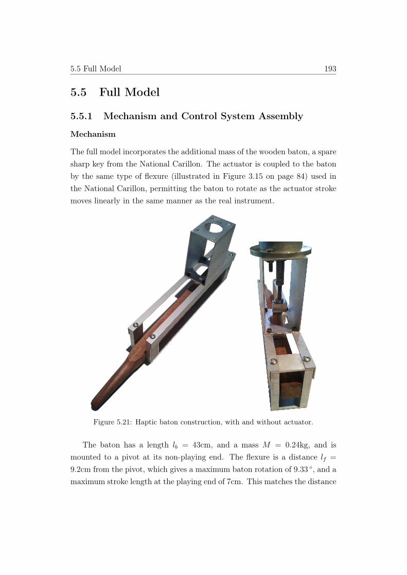
5.5 Full Model 193
5.5 Full Model
5.5.1 Mechanism and Control System Assembly
Mechanism
The full model incorporates the additional mass of the wooden baton, a sparesharp key from the National Carillon. The actuator is coupled to the batonby the same type of flexure (illustrated in Figure 3.15 on page 84) used inthe National Carillon, permitting the baton to rotate as the actuator strokemoves linearly in the same manner as the real instrument.
Figure 5.21: Haptic baton construction, with and without actuator.
The baton has a length lb = 43cm, and a mass M = 0.24kg, and ismounted to a pivot at its non-playing end. The flexure is a distance lf =
9.2cm from the pivot, which gives a maximum baton rotation of 9.33 ◦, and amaximum stroke length at the playing end of 7cm. This matches the distance
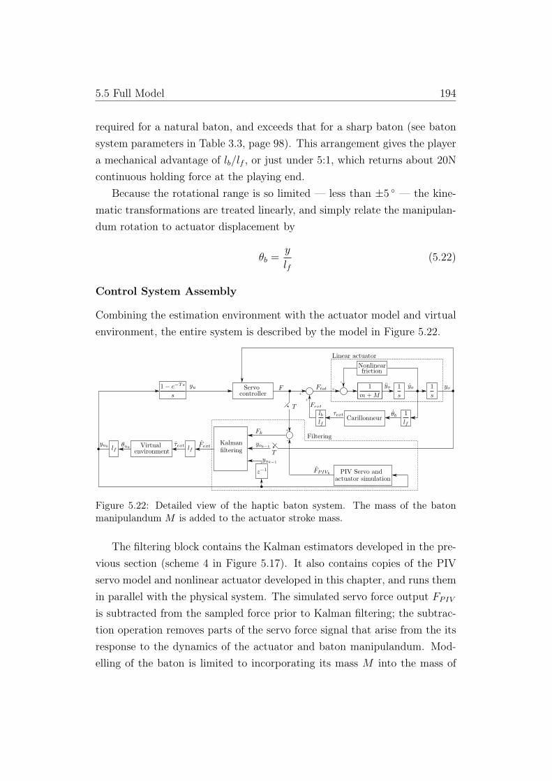
5.5 Full Model 194
required for a natural baton, and exceeds that for a sharp baton (see batonsystem parameters in Table 3.3, page 98). This arrangement gives the playera mechanical advantage of lb/lf , or just under 5:1, which returns about 20Ncontinuous holding force at the playing end.
Because the rotational range is so limited — less than ±5 ◦ — the kine-matic transformations are treated linearly, and simply relate the manipulan-dum rotation to actuator displacement by
θb =y
lf(5.22)
Control System Assembly
Combining the estimation environment with the actuator model and virtualenvironment, the entire system is described by the model in Figure 5.22.
++
+
-
+
-
Figure 5.22: Detailed view of the haptic baton system. The mass of the batonmanipulandum M is added to the actuator stroke mass.
The filtering block contains the Kalman estimators developed in the pre-vious section (scheme 4 in Figure 5.17). It also contains copies of the PIVservo model and nonlinear actuator developed in this chapter, and runs themin parallel with the physical system. The simulated servo force output FPIVis subtracted from the sampled force prior to Kalman filtering; the subtrac-tion operation removes parts of the servo force signal that arise from the itsresponse to the dynamics of the actuator and baton manipulandum. Mod-elling of the baton is limited to incorporating its mass M into the mass of

5.5 Full Model 195
the actuator stroke. The minor frictional elements arising from the rotationalpivot are ignored.
Software/Hardware
The equations constituting the virtual environment are coded into Matlab’sSimulink software. The Kalman filtering is coded in Matlab’s m-file code,and incorporated into the Simulink model as an embedded code function.This Simulink model is compiled into C-code for use on an xPC Targetmachine; the target machine in this application is an 2.8GHz x86 PC with2GB RAM, a National Instruments A/D card, and an ethernet port forcommunicating with a host machine, in this case a MacBook Pro runningWindows 7 in Boot Camp.
The BIOS on the target machine is configured to perform only criticaltasks, and the target machine is booted from a xPC Target DVD which con-tains a Simulink operating system. Once booted, an application is uploadedfrom the Matlab command line on the host computer, and then run nativelyon the target machine. This optimises execution times, our application runscomfortably at a sampling rate of 1 kHz. Data is logged on the host targetover the ethernet connection whilst the application is running.
5.5.2 Mass-spring-damper Simulation
The system is tested with a virtual environment consisting of a mass-spring-damper model described by the following equation of motion:
Iθ + bθ + kθ = τext (5.23)
where I = 0.05 kg ·m2 is the virtual moment of inertia, b = 0.2 N.m/(rad/sec)is the virtual damping, k = 50 N.m/rad is the virtual spring, and τext is thedriving torque applied by the user. This system is significantly underdamped(ζ = 0.06) and has an underdamped angular frequency of ω1 ≈ 31 rad/sec.
Because this system is underdamped, it oscillates for some time withoutexternal force. The low inertia also makes is responsive to small forces.

5.5 Full Model 196
This makes a good test environment for the efficacy of the force-sensing andfiltering environment. In particular, the servo will generate forces in the orderof ±4 N simply to keep the actuator oscillating; confusing these with user-applied force will make the system under-responsive at best, and unstable atworst. This simple system is also a good test because the servo control forceswill be very close to the system’s resonant frequency, because they will bedriving motion at that resonant frequency.
Plots
The following plots show the system performance in the mass-spring-dampersimulation, including measured position, measured force, simulated force,and the difference between the two (Figure 5.23). In Figure 5.24, the resultsfrom Kalman estimation of the force signal are shown. The filtered subtractedsignal is plotted against the filtered measured signal in order to demonstratethe significant removal of servo control forces due to the actuator.
2 4 6 8t HsecL
-40
-20
20
NMeasured force
(a) Measured force.
2 4 6 8t HsecL
-4
-2
2
4
NSimulated force
(b) Simulated force (FPIV ).
2000 4000 6000 8000t HsecL
-40
-20
20
NSubtracted force
(c) After subtraction (F ).
2 4 6 8t HsecL
-1.0
-0.8
-0.6
-0.4
-0.2
0.2
0.4
cmMeasured position
(d) Measured actuator displacement.
Figure 5.23: Mass-spring-damper control system response plots.

5.5 Full Model 197
2 4 6 8t HsecL
-30
-20
-10
NFiltered force
(a)
7.5 8.0 8.5 9.0t HsecL
-30
-20
-10
0
NFiltered force
(b)
1.2 1.4 1.6 1.8 2.0t HsecL
-12
-10
-8
-6
-4
-2
0N
Filtered force
(c)
2.5 3.0 3.5t HsecL
-2
-1
0
1
2N
Filtered force
(d)
Figure 5.24: Filtered force from mass-spring-damper simulation, with and withoutsubtracting simulated force FPIV (unbroken and broken, respectively).
The measured forces in Figure 5.23a are as noisy as expected, and thesimulated force FPIV is also quite noisy, mainly because of the low velocitiesin this simulation — the chirp signal simulations in §5.3.3 show that thePIV model becomes smoother at around 8–10 Hz. Beyond the stationarynoise, however, the force peaks associated with moving the actuator are quitevisible, particularly after large external force impulses at 3.5, 4 and 7 seconds.
It is impossible to visually discern any difference between the measuredforce before and after subtraction of the simulated force. However, afterfiltering through Kalman estimation, there is an obvious difference. Figure5.24 shows the results of filtering the measured signal without subtractingthe simulated force FPIV , and filtering the measured signal after subtractingFPIV .
The full plot in Figure 5.24a shows that during periods of obvious exter-nal force application, the force readings are quite similar. The zoomed plots,focusing on the very start of the signal, and during the final force impulse,

5.6 Summary 198
show that during periods of no external force input, the cancellation is effec-tive. Some oscillatory forces remain in the subtracted signal — this is due toa combination of inaccuracies in the PIV model, and the altered dynamicsof the actuator model now that it is coupled to the manipulandum.
5.6 Summary
This chapter has described the development of a haptic device for admittancedisplay. Equations of motion are arranged in Simulink for forward dynamicssimulation, taking user-applied force as an input and returning desired batonposition as an output. Force sensing is not performed using any additionalforce sensors, rather, the current signal from the servo controller to the actu-ator is monitored and filtered to extract the user-applied force. This filteringis based on a servo controller and actuator simulation which predicts forcetransients due to position commands, and Kalman estimators which smooththe remaining noisy force signal.

Chapter 6
The Data Set: The NationalCarillon
This chapter presents the myriad data sets associated with the NationalCarillon. These include variation in physical characteristics across the rangeof the instrument, variation in force-feedback, and variation in baton motion.
The categorisation of these features is referred to as the haptic signa-ture, and it distinguishes one carillon from another. The haptic signaturecomprises a set of measurements which includes static and dynamic force-feedback at the baton’s playing end, and its motion in response to appliedforces. Motions are measured under static load — i.e. with a constant zeroand non-zero force — and forces are measured at zero velocity with a rangeof baton displacements; for batons 1–17, force-feedback and motion are alsorecorded during repeated strokes of differing velocities.
The haptic signature provides a roadmap to the development and im-plementation of a computational model for haptic simulation of an arbitrarybaton. The model developed in Chapters 3 and 4 is populated with numericalvalues based on initial estimates, simulation and comparison against motionand force-feedback provided by the haptic signature.
During the first part of this chapter, a scaling function for variation inclapper properties is derived from the existing literature on the scaling ofcarillon bells. This scaling function is a good predictor for clapper mass, an
6.1 Variation in Physical Parameters 200
otherwise difficult quantity to measure. Variation in clapper mass, though,explains little of a baton’s dynamics; an estimate of clapper mass is a valuablepredictor of total mechanical inertia (associated with forces due to accelera-tion) but provides no information about dynamic characteristics arising fromfriction (velocity/position), and gravity and/or springs (position). This ne-cessitates some form of system identification and modelling based on observedmotion and force-feedback which accounts for forces arising from velocity andposition, and for motion arising from applied forces.
The second part of this chapter identifies and presents haptic signaturesfor a range of representative batons across the instrument, providing a senseof the dynamic variation and the nature of the data encapsulated in the hapticsignature. The data in §6.3.3 is a good demonstration of the extent to whichforce-feedback is a function of position, velocity, and stroke direction. Afterleast-squares fitting, the linear model developed in Chapter 4 is shown tocapture a significant portion of dynamic force-feedback of individual batons.
However, the linear fit for baton 7’s haptic signature fails to capture asignificant nonlinearity, a mechanical detent midway through its stoke. Anovel implementation of the Discrete Wavelet Transform is used to modelthis feature. In this case, the haptic features are a function of both positionand velocity, with a position-related detent and a smoothing factor relatedto velocity.
6.1 Variation in Physical Parameters
This section contains data collected relating to the variation in clapper rodlengths across the National Carillon; through measurement and analysis itis shown that clapper rod lengths and clapper masses and dimensions canbe predicted by established principles governing the scaling of carillon bellsthemselves. Baton and crank variation is ignored here as baton dimensionsare unchanged across the carillon, once accounting for the difference betweennatural and sharp batons, and cranks come in only two sizes with those forbells 40 and up a little smaller than the rest.
Figure 6.1 is a representation of a clapper part. While each clapper part
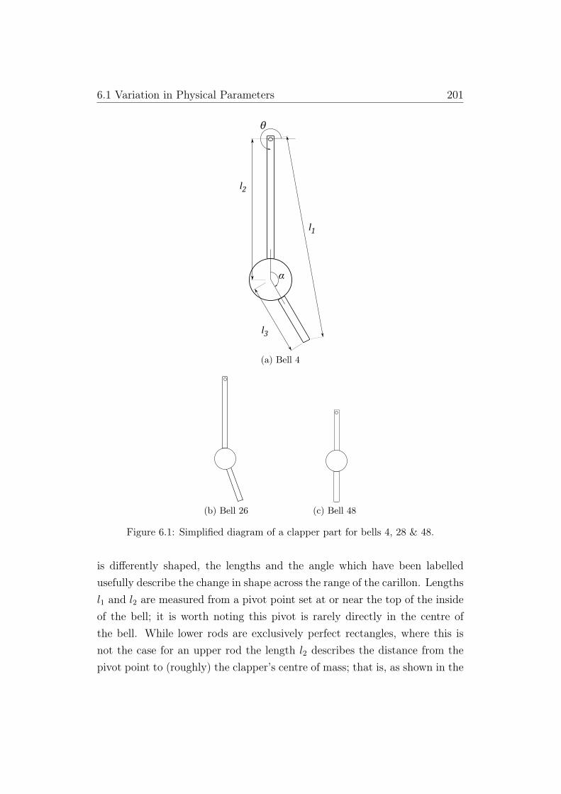
6.1 Variation in Physical Parameters 201
l2
l3
l1
α
θ
(a) Bell 4
(b) Bell 26 (c) Bell 48
Figure 6.1: Simplified diagram of a clapper part for bells 4, 28 & 48.
is differently shaped, the lengths and the angle which have been labelledusefully describe the change in shape across the range of the carillon. Lengthsl1 and l2 are measured from a pivot point set at or near the top of the insideof the bell; it is worth noting this pivot is rarely directly in the centre ofthe bell. While lower rods are exclusively perfect rectangles, where this isnot the case for an upper rod the length l2 describes the distance from thepivot point to (roughly) the clapper’s centre of mass; that is, as shown in the

6.1 Variation in Physical Parameters 202
figure.
6.1.1 Scaling of Bells
From the analyses of Rossing [107], Bigelow [12] and Lehr [77] we know thescaling of carillon bells can be more or less described by the expressions:
r = k1
f(6.1a)
m = c r3 = c
(k
f
)3
(6.1b)
where f is the fundamental frequency of the bell, r is its large radius, m isits mass, c and k are scaling factors, and c/k is mostly constant for smalland large bells across the carillon range.
Scaling bell dimensions by 1/f (Eq. (6.1a)) was common practice for bellfounders in the 15th and 16th centuries [121], but it lead to treble bells thatwere too small to radiate sound effectively. We see from the cubed frequencyterm in Eq. (6.1b) that treble bell masses are very small indeed where thisscaling is rigidly followed, so from the 17th century bell founders increasedthe size of their treble bells. In a plot reproduced here, Rossing shows thatthe clapper height, diameter and thickness of three 17th-century Hemonycarillons are related to frequency by 1/f until about G4 [107, p. 66].
Importantly, each of the bell features plotted in Rossing’s figure areroughly proportionate to bell height even after diverging from 1/f ; this rela-tion allows us to link clapper features to the equations describing bell scaling.In particular, the clapper length l1 is correlated with bell height, and clappermass is correlated with bell mass for acoustical reasons.
Another observation to take from Figure 6.2 is that, particularly in thehighest bells, changes in dimensions are not strictly monotonic.
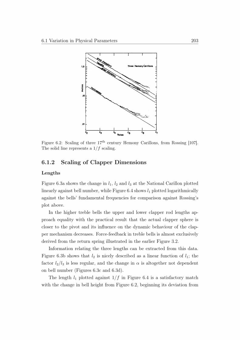
6.1 Variation in Physical Parameters 203
Figure 6.2: Scaling of three 17th century Hemony Carillons, from Rossing [107].The solid line represents a 1/f scaling.
6.1.2 Scaling of Clapper Dimensions
Lengths
Figure 6.3a shows the change in l1, l2 and l3 at the National Carillon plottedlinearly against bell number, while Figure 6.4 shows l1 plotted logarithmicallyagainst the bells’ fundamental frequencies for comparison against Rossing’splot above.
In the higher treble bells the upper and lower clapper rod lengths ap-proach equality with the practical result that the actual clapper sphere iscloser to the pivot and its influence on the dynamic behaviour of the clap-per mechanism decreases. Force-feedback in treble bells is almost exclusivelyderived from the return spring illustrated in the earlier Figure 3.2.
Information relating the three lengths can be extracted from this data.Figure 6.3b shows that l2 is nicely described as a linear function of l1; thefactor l2/l3 is less regular, and the change in α is altogether not dependenton bell number (Figures 6.3c and 6.3d).
The length l1 plotted against 1/f in Figure 6.4 is a satisfactory matchwith the change in bell height from Figure 6.2, beginning its deviation from

6.1 Variation in Physical Parameters 204
è
è
è
è
è
è
è
è
è
è è è
�
�
�
�
�
�
�
�
�
��
�
ò
ò
ò
ò òò ò
ò òò ò ò
l1è
l2�
l3ò
10 20 30 40 50bell #
0.2
0.4
0.6
0.8
1.0
1.2
1.4
m
(a) Linear plot, l1, l2, l3
ò
ò
ò
ò
ò
ò
ò
ò
ò
òò
ò
0.2 0.4 0.6 0.8 1.0 1.2 1.4l1 HmL
0.2
0.4
0.6
0.8
1.0
l2 HmL
(b) l2 as a function of l1
è
è
è
è
è è
è
è
è
è
è
è10 20 30 40 50bell #
1.5
2.0
2.5
3.0
3.5
l2�l3
(c) l2/l3
èè
è
è
è
è
è
è
è
è
èè
10 20 30 40 50bell #
150
160
170
180
Α °
(d) Change in α
Figure 6.3: Clapper length dimensions over the carillon range.
this line just after C4 and then barely changing after C6. The closeness ofthis match is a little surprising given that the upper clapper rod pivot israrely centred in the bell.
An additional dashed line is included that shows the least-squares lin-ear fit, achieved by changing the slope of the line by having 1/f 0.78. This

6.1 Variation in Physical Parameters 205
slope will be used for fitting parameters to the linear model for carillonneur-evaluation.
è
è
è
è
è
è
è
è
è
èè
è
l1è
1� f
1� f 0.78
100 1000500200 2000300150 1500700
0.10
1.00
0.50
0.20
0.30
0.15
1.50
0.70
G2 C3 C4 C5 C6 C7
f HHzL
l 1Hm
L
Figure 6.4: Clapper length l1 log plot across the carillon range.
Clapper Rotation
The total extent of clapper rotation was also measured — i.e. the differencein θ (Figure 6.1a) with the clapper touching the inside of the bell wall, andat rest some 3–4 cm away from the bell wall; the results are plotted below inFigure 6.5 as a function of bell number and l1.
Figure 6.5a shows a near-linear relationship between total rotation andbell number.
A more interesting result is shown in Figure 6.5b, where rotation is shownas a function of l1; this is yet another inversely proportional dimensionalscaling, with
θtot ∝1
l1(6.2)
The above expression is derived from the relationship dtot = l1 θtot wheredtot is the absolute distance travelled by the clapper tip; because l2 is alinear function of l1 this relationship also governs the distance travelled bythe actual clapper sphere. As a question of carillon design, it is importantthat dtot remain constant across the carillon range (see §3.5.1).

6.1 Variation in Physical Parameters 206
ò ò
ò
ò
òò
ò
ò
ò
ò
ò
ò
10 20 30 40 50bell #
2
4
6
8
10
Θtot °
(a) θtot against bell
òòò
ò
òò
ò
ò
ò
ò
ò
ò
0.2 0.4 0.6 0.8 1.0 1.2 1.4l1HmL
2
4
6
8
10
Θtot °
(b) θtot against l1
Figure 6.5: Total clapper rotation over the carillon range.
Clapper Masses and Force
Another useful observation is an extension of the second expression in Eq.(6.1), m = c (k/f)3, and its predictive properties for clapper mass acrossthe carillon range. Based on similarities in dimensional scaling for clapperlengths and bell properties, it is expected that clapper masses are similarlyrelated, with mC being roughly proportionate to bell mass m.
While determining mC empirically is difficult given irregular clappershapes and clappers permanently fixed at either end to the clapper rods,the static force FC at the tip of the lower clapper rod — that is, at a dis-tance l1 from the pivot — required to hold the clapper against the bell wallcan be measured. Through the expression for torque due to gravity actingon clapper mass at a length l2 and an angle θ,
τ = −g l2mC cos(θ)
where g and θ are constant, and l2 is a function of l1 which is related linearlyto r, Eq. (6.1) can be extended to describe clapper mass scaling:
τ = c
(k
f
)3
(6.3)
This scaling is plotted against the measured values for torque in Figure6.6 and we see a divergence from 1/f 3 very similar to that from 1/f for bellproperties in Rossing’s Figure 6.2, and Figure 6.4 plotting l1 over frequency.

6.1 Variation in Physical Parameters 207
Again, as with clapper lengths against frequency, as slightly smaller exponentfor the frequency term gives a better fit, in this case changing torque is moreaccurately described as proportional to 1/f 2.
è
è
è
è
è
è è
è
è
è èè
Τ H f Lè
1� f 3
1� f 2
1000500200 2000300150 1500700f HHzL
0.1
1
10
100
Τ HN.mL
Figure 6.6: Torque about clapper pivot against bell frequency. Includes 1/f3 and1/f2.
As a further confirmation of the predictive qualities of these equations,torque is described as a function of length l1, in their respective capacitiesas proxies for bell mass and bell radius. Figure 6.7 plots both the measuredpoints and the best fit for a curve of the form
τ ∝ l31 (6.4)
which is analogous to Eq. (6.1b), m = cr3.The straight line is quite a good fit for the heavier bells, with lighter bells
deviating similarly to how bell sizes deviate from 1/f .
Summary
This section has demonstrated that clapper rotation and torques (and massesgiving rise to those torques) can be expressed as functions of the length l1
between the clapper pivot and the tip of the lower clapper rod where it iscoupled to the crank. This length has in turn been shown to be inverselyproportional to bell frequency f .

6.2 Variation in Baton Motion 208
ò
ò
ò
ò
ò
òò
ò
ò
òò
ò
1.000.500.20 0.30 1.500.70l1 HmL
0.5
1.0
5.0
10.0
50.0
100.0
Τ HN.mL
Figure 6.7: Torque about clapper pivot against clapper length l1.
Finally, the clapper dimensions in the National Carillon are describedusing these relations and the following constants:
θtot =0.32
l1(6.5a)
τ = 54 l31 (6.5b)
l1 =59
f 0.78(6.5c)
6.2 Variation in Baton Motion
A striking feature of the carillon keyboard is the length of time a batonremains in motion after a note has been played and the carillonneur nolonger applies any force, or influences the baton’s motion in any way. Fromthe point of view of the engineer the measurement and categorisation of abaton’s free motion provides a convenient insight into the dynamics of therest of the carillon mechanism. In this section focuses on baton motion freeof any force input, and motion with a static force due to an attached mass.
An orientation sensor is used to measure the change in rotation overtime at different parts of the system.1 The sensor is shown attached to a
1Xsens MTx Attitude and Heading Sensor, http://xsens.com/en/general/mtx.
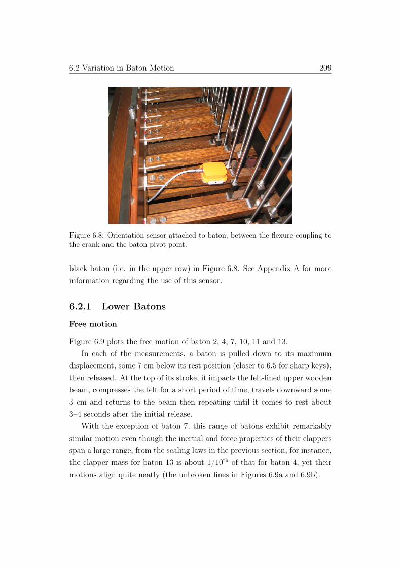
6.2 Variation in Baton Motion 209
Figure 6.8: Orientation sensor attached to baton, between the flexure coupling tothe crank and the baton pivot point.
black baton (i.e. in the upper row) in Figure 6.8. See Appendix A for moreinformation regarding the use of this sensor.
6.2.1 Lower Batons
Free motion
Figure 6.9 plots the free motion of baton 2, 4, 7, 10, 11 and 13.In each of the measurements, a baton is pulled down to its maximum
displacement, some 7 cm below its rest position (closer to 6.5 for sharp keys),then released. At the top of its stroke, it impacts the felt-lined upper woodenbeam, compresses the felt for a short period of time, travels downward some3 cm and returns to the beam then repeating until it comes to rest about3–4 seconds after the initial release.
With the exception of baton 7, this range of batons exhibit remarkablysimilar motion even though the inertial and force properties of their clappersspan a large range; from the scaling laws in the previous section, for instance,the clapper mass for baton 13 is about 1/10th of that for baton 4, yet theirmotions align quite neatly (the unbroken lines in Figures 6.9a and 6.9b).

6.2 Variation in Baton Motion 210
0.5 1.0 1.5 2.0 2.5 3.0t HsecL
-7
-6
-5
-4
-3
-2
-1
0
position HcmL
Baton 7
Baton 4
Baton 2
(a) Batons 2, 4 & 7.
0.5 1.0 1.5 2.0 2.5 3.0t HsecL
-7
-6
-5
-4
-3
-2
-1
position HcmL
Baton 13
Baton 11
Baton 10
(b) Batons 10, 11 & 13.
Figure 6.9: Free baton motion for lower batons; in each case the baton was heldto its maximum displacement (batons 11 & 13 are sharp keys with smaller keyfall)then released.
This is the key indication that free baton motion alone does not pro-vide enough information for simulating a baton’s dynamics; data in the nextsection shows that baton 4 requires over 12 N of force at its tip to holdkeep it depressed while baton 13 requires less than 6 N. However, free batonmotion is a useful initial corroboration of estimated simulation parameters,

6.2 Variation in Baton Motion 211
and probably the best observation against which to tune parameters likevelocity-dependant friction and energy transfer during debounce.
Motion under static load
A second observation of motion with the baton under a static load partlyaddresses the inconclusiveness of baton free motion as an observation againstwhich to tune simulation parameters. Such motion for batons 4, 7 and 10 isshown in Figure 6.10. This data was recorded by fixing a mass to the tip ofa baton then releasing it from the top of its stroke.
0.2 0.4 0.6 0.8 1.0 1.2t HsecL
-7
-6
-5
-4
-3
-2
-1
position HcmL
Baton 10 H1.25KgL
Baton 7 H1.7KgL
Baton 4 H2.5KgL
Figure 6.10: Batons 4, 7 & 10 motion under static load.
While the static load motions are useful for comparison against simulationresults, they are less useful for interpreting respective baton’s response toapplied force. However, they do serve as a check against false positives inparameter estimation that arise when matching free baton motion alone. Forthis reason static loads where chosen that lead to similar motions across thebaton range with each baton taking between 250–500 milliseconds to firstimpact.

6.2 Variation in Baton Motion 212
Disturbances in Motion
Rigorous force analysis is better done using methods described later in §6.3.3,however peculiarities found during that process are usefully cross-checkedagainst these static load plots, as well as picking up behavioural featuresmissed in that analysis. Baton 7 is a good example.
The dotted line in Figure 6.10 indicating motion for baton 7 with a 1.7Kgmass attached (≈16.5 N) is seen to accelerate faster than batons 4 or 10 inthe first 200 milliseconds before slowing down and being overtaken by baton4 then baton 10. A detent, or disturbance in motion due to some mechanicalcatch or resistance, is visible for baton 7 around the -3 cm mark, hinting atsome non-linear increase in force-feedback around this point.
Looking forward to Figure 6.23 on page 229 there is indeed a jump in themagnitude of force-feedback at the -3 cm mark during a downward strokethat is a non-linear function of position.
6.2.2 Middle Batons
Batons 21–34 are characterised by the weak or non-existent influence of for-ward and return springs; springs are coupled to the clapper mechanisms21–24 but the coupling cable is slack during motion, and the springs exertno force on the clapper mechanism.
A clear feature of these figures is the similarity of response to a staticload; this highlights the need to consider both free motion and motion understatic load in tandem. Figures 6.11a and 6.11b relating to batons 29, 30and 31 show that a set of batons may have a uniform response to an equalload whilst exhibiting dissimilar free motion. The free motion plots for thesebatons also demonstrate that proximity of baton number is no predictor forfree motion.
Figures 6.11c and 6.11d, on the other hand, demonstrate the influenceof impact constraints. Whilst batons 21 and 24 have similar periods, theiramplitudes on return from impact during free motion are clearly different,with baton 24 about 1 cm lower on each rebound.
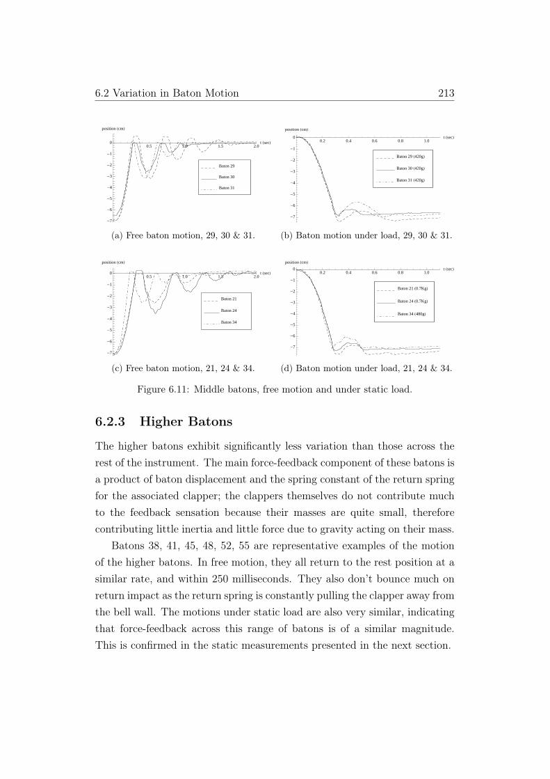
6.2 Variation in Baton Motion 213
0.5 1.0 1.5 2.0t HsecL
-7
-6
-5
-4
-3
-2
-1
0
position HcmL
Baton 31
Baton 30
Baton 29
(a) Free baton motion, 29, 30 & 31.
0.2 0.4 0.6 0.8 1.0t HsecL
-7
-6
-5
-4
-3
-2
-1
0
position HcmL
Baton 31 H420gL
Baton 30 H420gL
Baton 29 H420gL
(b) Baton motion under load, 29, 30 & 31.
0.5 1.0 1.5 2.0t HsecL
-7
-6
-5
-4
-3
-2
-1
0
position HcmL
Baton 34
Baton 24
Baton 21
(c) Free baton motion, 21, 24 & 34.
0.2 0.4 0.6 0.8 1.0t HsecL
-7
-6
-5
-4
-3
-2
-1
0
position HcmL
Baton 34 H480gL
Baton 24 H0.7KgL
Baton 21 H0.7KgL
(d) Baton motion under load, 21, 24 & 34.
Figure 6.11: Middle batons, free motion and under static load.
6.2.3 Higher Batons
The higher batons exhibit significantly less variation than those across therest of the instrument. The main force-feedback component of these batons isa product of baton displacement and the spring constant of the return springfor the associated clapper; the clappers themselves do not contribute muchto the feedback sensation because their masses are quite small, thereforecontributing little inertia and little force due to gravity acting on their mass.
Batons 38, 41, 45, 48, 52, 55 are representative examples of the motionof the higher batons. In free motion, they all return to the rest position at asimilar rate, and within 250 milliseconds. They also don’t bounce much onreturn impact as the return spring is constantly pulling the clapper away fromthe bell wall. The motions under static load are also very similar, indicatingthat force-feedback across this range of batons is of a similar magnitude.This is confirmed in the static measurements presented in the next section.

6.3 Haptic Signature 214
0.2 0.4 0.6 0.8 1.0t HsecL
-7
-6
-5
-4
-3
-2
-1
0
position HcmL
Baton 45
Baton 41
Baton 38
(a) Free baton motion, 38, 41 & 45.
0.2 0.4 0.6 0.8 1.0t HsecL
-7
-6
-5
-4
-3
-2
-1
0
position HcmL
Baton 45 H480gL
Baton 41 H280gL
Baton 38 H480gL
(b) Baton motion under load, 38, 41 & 45.
0.2 0.4 0.6 0.8 1.0t HsecL
-6
-4
-2
0
position HcmL
Baton 55
Baton 52
Baton 48
(c) Free baton motion, 48, 52 & 55.
0.2 0.4 0.6 0.8 1.0t HsecL
-7
-6
-5
-4
-3
-2
-1
0
position HcmL
Baton 55 H280gL
Baton 52 H280gL
Baton 48 H280gL
(d) Baton motion under load, 48, 52 & 55.
Figure 6.12: High batons, free motion and under static load.
The key issue in modelling these batons is differentiating them from thosein the upper-middle range, with similar mass but without return springs. Inconversation with carillonneurs at the National Carillon, they described thesehigher batons as being ‘harder’ than those in the middle of the range. My ownimpression is that the constant return spring stops the baton from leavingthe hand during a downward stroke, creating a constant sensation of touchand little of the pliability of a clapper without return springs, which have agreater tendency to swing away from the hand during motion due to inertia.
6.3 Haptic Signature
In this section the haptic signature of the carillon is made up of the collectedhaptic signatures of its batons; in turn, batons are characterised by theirstatic and dynamic force-feedback properties, and their dynamic behaviourwhen not in contact with the carillonneur.

6.3 Haptic Signature 215
The force-feedback felt by a carillonneur at the baton is considered in twoways:
1. Static — the reaction force as the baton is held still at the top then thebottom of its stroke, with a measurement also taken at the mid-pointon the way down and on the way up; and
2. Dynamic — the continuous change in force as the baton is pressed tothe bottom of its stroke, then gradually allowed to return.
Static measurements facilitate an analysis of the change in force-feedbackacross the range of the carillon; dynamic measurements provide an insightinto force-feedback as experienced by a carillonneur, and serve as a check forthe haptic model developed over the course of this thesis.
6.3.1 Static Force-feedback
During early testing of the prototype baton, carillonneur Timothy Hurddemonstrated a technique carillonneurs employ when getting a feel for anew instrument: he placed his fist near the tip of the baton, then let thenatural weight of his arm force the baton downward a short distance, some5–10 mm. He mediated the ‘natural weight’ of his arm depending on thebaton’s heaviness, and this weight is learned as a starting force with whichthat particular baton must be engaged just prior to a stroke.
This position just below the baton’s resting position is the point in thestroke where the carillonneur applies a maximum force, rather than crashingdown onto the baton while it is totally at rest and at zero displacement.This technique mitigates the force-feedback due to clapper inertia, and avoidsgenerating backlash in the cable linking the baton to the crank.
This position is referred to as the resting position, and the force requiredto get the baton there the resting force, which is slightly greater than theforce required to displace the baton at all. This resting force is recordedby observing the reaction force from a force transducer (force measurementdevice) while keeping the baton depressed by some 5–10 mm. The forcerequired to hold the baton at maximum displacement at the bottom of its

6.3 Haptic Signature 216
stroke is also recorded. The difference between these two forces is a con-venient way of considering the change in force-feedback across the carillon;measurements are shown in Figure 6.13.
•
•
•
••
• •
•
•• •
• ••
•• • • • • • • • • • • • • • • • •
• • • • • • • • • • • • • • • • • • • • • ••
•
•
•
••
•
•
•
•
• •
• ••
•• • • • •
• • • • • • • ••
• • • • ••
• ••
• • • • • • • • • ••
••
• • ••
10 20 30 40 50bell #
-20
-15
-10
-5
0
F HNLForce-feedback at baton tip, all bells
Figure 6.13: Static force-feedback measured at the baton tip. The upper line showsthe resting force; the lower the force when the baton is fully depressed. Verticallines join the points as a visual aid.
The unevenness in this graph is partly because natural and sharp batonsare displayed adjacently. Figure 6.14a visually separates the force-feedbackof natural and sharp batons.
Lower Batons
Visible in Figure 6.14a, particularly in the the lower third of the instrument’srange, is the tendency for sharp batons to be heavier than adjacent naturalbatons, and when the two groups are separated it is clear that the change inforce within the groups themselves is not monotonic. Further, the magnitudeof force-feedback hardly changes after bell 20; the difference in haptic feelfor these higher bells is mainly the result of the decreasing inertia associatedwith smaller clappers.
The force required to hold the set of batons 1–19 at bottom is plottedlogarithmically2 against bell frequency in the scatter plot in Figure 6.14b;
2Force values are inverted and made positive for use with a logarithmic plot.

6.3 Haptic Signature 217
sharp top
natural top
sharp bottom
natural bottom
10 20 30 40 50bell #
-20
-15
-10
-5
F HNLForce-feedback at baton, by baton type
(a) Static force-feedback at baton tip, by baton type.
è
è
è
è
è
è
è
è
èè è
é
é
é
é
é
é
é
é
é
é
éé
F HÛ�ÙLè
F IÚMé
F HÛ�ÙL= 1� f 1.78
F IÚM= 1� f 1.70
F= 1� f 1.74
100 200 300150
10.0
5.0
20.0
3.0
15.0
7.0
G2 H1L C3 H5L G3 H12L C4 H17L
f HHzL
-F
HNL
baton H#L
(b) Force (inverted for log. plot) to hold baton at bottom, bells 1–19.
Figure 6.14: Static force-feedback at the baton tip, arranged by natural and sharpbatons, and then logarithmically against frequency for bells 1–19.
natural and sharp baton forces are shown and fitted separately, along with afit for all batons.
In each case, the force is inversely proportional to frequency and a goodfit is achieved using an expression of the form:
F (f) = c1
fx(6.6)

6.3 Haptic Signature 218
with only a slight difference in x and c for sharp and natural batons — sharpbatons are roughly 1.2 N heavier than natural batons for the lowest fewbatons, and this difference decreases to 0.5 N by baton 13. Numerical valuesfor x and c when considering sharp and natural batons together naturallyfall between the individual values for sharp and natural batons.
While this generalisation is useful, the scatter plot itself shows that theextent of variation can be much larger than predicted by the logarithmicfits: the 2nd sharp baton (6), for instance, is much lighter than expectedconsidering its neighbouring sharp batons.
Force analysis alone provides little insight into the haptic feel of the higherbatons. However, two further static measurements illuminate a little moreof dynamic properties of force-feedback in individual batons.
6.3.2 Mid-point Static Force-feedback
Along with measuring the static forces at the top and bottom of a baton’sstroke, two measurements are taken midway through the stroke, first duringdownward motion then as the baton returns. Figure 6.15 includes thesemeasurements.
Force-feedback at the mid-point is consistently greater during downwardmotion than upward motion, and the difference between force-feedback dur-ing downward and return motion is quite regular. Excluding the lowest tenbatons, the mean difference for batons 10–55 is 0.6 N, with a mean deviationof 0.2 N. The mean difference for the lowest ten batons is closer to 1.25 N,with a mean deviation of 0.7 N.
This difference is a guide to the influence of friction, a constant forceduring motion which opposes motion. As an element of the classical dryfriction model this force is called dynamic or kinetic friction and is describedas Fk = µkFN , where FN is the normal force between two objects movingrelative to each other and µk is the coefficient of dynamic friction. In theKarnopp model, µkFN is bundled into a single coefficient velocity-directionterm, Cn sgn(v).
This dynamic friction is in large part comprised of rubbing between alu-

6.3 Haptic Signature 219
è
è
è
è
è
èè
è
è
èè
èè
è
è
è è è è èè è è
è èè
è è èè
èè
è è è è è èè è è è è è è
èè
è èè è
èè
è
è
è
è
è
è
è
è
è
è
è
è è
è è
è
è
èè è è
è
èè è è
èè
èè
è
è è è è è
è
è è
è
è è èè
èè è
èè
è
è
è
è
èè
è
è
10 20 30 40 50bell #
-20
-15
-10
-5
0
F HNLForce-feedback at baton tip, all bells
(a) All batons.
è
è
è
è
è
èè
è
è
èè
è
è
è
è
è
è
è
è
è
è è
ô
ô
ô
ô ô
ô
ôô
ô
ô
ô
ò
ò
ò
ò
ò
ò
ò ò
ò
ò
ò
2 4 6 8 10bell #
-20
-15
-10
-5
0
F HNLForce-feedback at baton tip, bells 1-10
(b) Batons 1–10; arrows indicate downwardand upward strokes.
è
è
è
è
è
è
è
è è è è è
è èè
è è
è
èè è
è
è
è
èè
èè è è
è èè
èè è
è
è
è
è è
èè
è
è
è
è
è
èè
è è
è
è
è
èè è
è
è
èè è
è
è
è
è
è
è è è è è
è
èè
è
è èè
è
è
èè
è
è
è
è
è
è
è
è
è
è
20 30 40 50bell #
-8
-6
-4
-2
0F HNL
Force-feedback at baton tip, bells 11-56
(c) Batons 11–55.
Figure 6.15: Static force-feedback at the baton tip, including midpoints.
minium and wool felt components, and is quite audible in the clavier room.Attached to both sides of the baton, two small pieces of felt (≈ 3 cm2) sepa-rate it from the aluminium cylinders holding the baton in place; and, the rodlinking the baton to the crank in the belfry is permanently pressed againstguide holes lined by felt. The normal force at each of these interactionsis largely independent of other forces in the mechanism, hence the limitedvariation in the midpoint difference forces.
The frictional properties of felt are quite sensitive to pressure applied bythe object in relative motion; Brown [17] shows that the kinetic coefficientof friction increases exponentially with pressure. It is conceivable that someof the variation in the midpoint differences are due to slight irregularities inbaton alignment, or lateral baton motion which increases pressure between

6.3 Haptic Signature 220
è
è è
è
è
è è
è
è
è
è
è è
è
è
è
è
è è
è
è
è
è
è
è
è
è
è
è è
è
è
è
è
è
è
è è
è
è
è
è
è
è
è
è
è
è
è
è è
è
è
è
è
10 20 30 40 50bell #
-3.5
-3.0
-2.5
-2.0
-1.5
-1.0
-0.5
D Fmid HNLDifference between down�up-ward midpoints
(a) Differences between midpoints.
ò
ò
ò
ò
ò
ò
ò
ò
ò
ò
ò
ò
ò
òò
ò
ò
ò
ò
ò
ò
ò
ò
ò
ò
ò
ò
ò
ò
ò
ò
ò
ò
òò
ò
ò
ò
ò
òò
ò
ò
ò
ò
ò
ò
ò
ò
ò
ò
òò
ò
ò
ô
ô
ôô
ô
ô
ô
ô
ô
ô
ô
ô
ô
ô
ô
ô
ô
ô
ô
ô
ôô
ô
ôô
ô
ô
ô
ô
ô
ô
ô
ô
ô
ôô
ô
ô
ôô
ô
ôô
ô
ô
ô
ôô
ô
ôô
ô
ô
ô
ô
10 20 30 40 50bell #
-0.6
-0.4
-0.2
Fmid
Fmax - Fmin
Midpoints placement in force range
(b) Midpoints related to force range; respec-tive means given by dashed lines.
Figure 6.16: Static force-feedback, midpoint analysis.
the felt and one of the cylinders.The increased differences for baton 1–10 is are most likely due to signif-
icantly greater normal force at the pivot point for their respective clappers.Figure 6.6 shows that clapper mass decreases by 1/10th from bell 2 to bell10; it takes the rest of the instrument’s range for clapper mass to drop by anequivalent proportion.
Finally, Figure 6.16b shows that the midpoint force is roughly similar as aproportion of the total force range for every baton; the average force-feedbackmidway during a downward stroke is about 60% of the entirety of that range,and the midpoint during an upward stroke about 35%.
6.3.3 Dynamic Force-feedback in Lower Batons
The analysis in this section is inspired by the work of Maclean [84], andwith Swindells [117] on capturing the dynamics of mechanical knobs using apurpose-built haptic camera, and Weir [128] on capturing and describing thefeel of switches using methods that together encapsulate what he describesas a haptic profile. Key to both works is the concept of exploring dynamicrelationships in domains other than time.
Setting aside forces due to acceleration and inertia,3 coefficients are de-3The recorded motions deliberately avoid large accelerations. Also, clapper, crank and
baton mass are the few parameters that can be predicted from the work in the previoussection.

6.3 Haptic Signature 221
termined for the velocity, position and constant terms in a spring-dampermodel.
Motion and force data are separated into two bins of upward and down-ward strokes to account for motion-dependant friction coefficients in theKarnopp friction model [96]; velocities less than 0.005 m/sec are deletedbecause they are dealt with by the stiction part of the Karnopp model. Co-efficients for position (spring), velocity (damper) and a constant offset aredetermined for each bin using linear fitting functions in Mathematica.4
Baton 4
Figure 6.17 plots baton position and force against time to give an indicationof the type of action used to collect the data. A player was instructed todepress the baton to its maximum displacement and then allow it to returnto rest while staying in contact with the baton at all times; the procedurewas repeated several times with increasing velocity.
0 5 10 15
0
-1
-2
-3
-4
-5
-6
-7
0
3
7
10
14
17
21
24
t HsecL
posi
tion
HcmL
forc
eHN
L
force
position
Figure 6.17: Force/position time profile, baton 4.
Removing chronology as a feature of interest, Figure 6.18 presents a morenuanced picture of the relationship between position and force in baton 4.
4Force data in this section was captured using a force sensing resistor attached to theplaying tip of the baton. See Appendix A for information regarding calibration of thissensor.

6.3 Haptic Signature 222
Time is still referenced with the inclusion of colour markers indicating ve-locity, which are organised such that ‘hot’ colours indicate negative velocity(downward motion) and ‘cool’ colours represent positive velocity, with vari-ations in velocity marked by the colours in between.
4.5 cm�sec
-4.5 cm�sec
5 10 15 20 25force HNL
-7
-6
-5
-4
-3
-2
-1
position HcmLBaton position as a function of force
Figure 6.18: Baton position as a function of force, baton 4. The colours indicatevelocity: hot colours indicate negative velocity (downward motion) and cool coloursindicate positive velocity.
Among several features to note here is the strong dependance on boththe direction and magnitude of velocity, suggesting the existence of bothdynamic and viscous friction in the system. The colours are grouped in sucha way as to illuminate that force at a particular position is likely to be higherduring the downward stroke than the upward stroke. Further, we see that thecurves do not align, and the magnitude of force-feedback during a downwardstroke is greater if the velocity of the stroke is greater. This relation is not asstrongly prevalent during an upward stroke, with those curves more tightlygrouped together even though the velocity range is as broad as for downwardmotion.
Figure 6.19 swaps the axes from Figure 6.18 such that force is shown asa function of position, and discards points at the maximum and minimum

6.3 Haptic Signature 223
baton displacements in order to focus on the region of change.5 It also sep-arates the data points into two groups which are determined by the velocitydirection — red data points indicate downward motion, and blue data pointsindicate upward motion. A linear regression line was determined for eachof the groups and included in the plot with matching colours; note that thevelocity — whilst no longer coloured — is encoded in the spacing betweendata points, i.e. larger spacing equals greater velocity.
è
èè
è
è
è
è
è
è
èèèèè
èè
èè
èè
èè
èè
èèè è èè
è
èè
è èè è
èè
èè
èè
è
è
èè
è
èè
èè
èè
èè
è è è è è è è è èè èè
èè
èè
èè
èè
èè
èè
èè
èèèèè è
èè
è èèèèèèè èè è è èèèèèè è è è èèèèèèèèè
è
è
èèèè
è
èèè
è
è
è
è
è
èèèèèèèèè
èèèèèè
èèè
èèè
èè
èè
è
è
è
è
è
è
è
è
è
è
è
èè
èè
è
è
è
è
è
è
èè
èè
è
è
è
è
èè
èè
èè
èè
è
è
è
è
è
è
è
è
è
è
è
è
è
è è èè è è
èè
è
è
è
è
è
è
è
è
è
è
è
è
è
è
è
èè
èè
èè
è
è
è
è
è
è
è
è
è
è
è
è
è
è
è
è
è
è
è
è
è
è
èè
èè
èè
è
è
è
è
è
è
èè
è
è
è
è
è
èè
è
è
è
è
è
è
è
è
è
è
è
è
è
è
è
è
è
è
è
è
è
è
è
è
è
è
è
è
èè
èè
è èè
èè
è
èè
è
è
è
è
è
è
è
è
è
è
è
è
è
è
è
è
è
è
è
è
è
è
è
è
è
è
è
è
è
è
è
è
è
èè
èè
è
è
è
è
è
è
è
è
è
è
è
è
è
è
è
è
è
è
è
è
è
è
è
èè
è
è
è
è
èèèèèèèèèèèèèèèèèèè
èèèèèèèèèèèè
èèèè
èèèè
èèè
èè
èè
èèèèèèèèèèèè
èè
èè
èè
èè
èè
èè
èè
èè
èè
èè
èè
èè
èèè
èè
èè
è
èè
è
èè
èè
èè
èè
èèèèèèèèèèèè
èè
èè
èè
èè
èè
èè
èè
èè
èèè
èè
è
è
è
è
è
è
è
è
è
è
è
è
èèèè
èèèèèèèèèèèèèèèè
èè
èè
èè
èè
èè
è
è
è
èè
èèè
èè
èè
èè
èè
è
èè
è
èè
è
è
è
è
èè
èè
èè
èè
èèèèèèè
èè
è
èè
èè
èè
è
è
è
è
è
è
è
è
è
è
è
è
è
è
è
è
è
è
è
è
è
èè
èè
èè
èè
èè
èè
èè
èè
è
è
è
è
è
è
è
è
è
è
è
è
è
è
è
è
è
è
è
è
è
è
è
è
è
è
è
è
è
è
è
è
è
è
è
è
è
è
è
èè
èè
èè
èè
èèèèè
èè
èè
è
è
è
è
è
è
è
è
è
è
è
è
è
è
è
è
è
è
è
è
è
è
è
è
è
è
è
è
è
èè
èè
èè
è
è
è
è
è
è
è
è
è
è
è
è
è
è
è
è
è
è
è
è
è
èè
è
è
è
è
è
èè
èè
èè
è
è
è
è
è
è
è
è
è
è
è
è
è
è
è
è
è
è
è
downward
upward
-7 -6 -5 -4 -3 -2 -1position HcmL
2
4
6
8
10
force HNLBaton force as a function of position
Figure 6.19: Baton force as a function of position, baton 4, with two linear regres-sion lines for downward and upward motion.
Combining the two regression lines into a case statement, an expressionfor force at any particular time based on position and a force offset associatedwith the direction of motion is given by:
Foff(x, t) =
2.1 x(t) < 0
0.7 x(t) > 0
F (x, x, t) = kx(t) + Foff(x, t) (6.7)
where k is close to equal for both lines, at approximately 1.25.The R-Squared (R2) values are 0.86 and 0.91 for downward and up-
ward motions, respectively, and they indicate the proportion of variabilityin the samples accounted for by the linear regression; i.e., how well the force-
5Hence the lines terminating at points other than the maximum and minimum posi-tion/force.

6.3 Haptic Signature 224
è
èè
è
è
è
è
è
è
èèèèè
èè
è
è
èè
èè
èè
èèè è è
èè
èè
è èè è
èè
èè
èè
è
è
èè
è
èè
èè
èè
èè
è è è è è è è è èè èè
èè
èè
èè
èè
èè
èè
èè
èèèèè è
èè
è èèèèèèè è è è è èèèèèè è è è èèèèèèèèè
è
è
èèèè
è
èèè
è
è
è
è
è
è
èèèèèèèè
èèèèèè
èèè
èèè
èè
èè
è
è
è
è
è
è
è
è
è
è
è
èè
èè
è
è
è
è
è
è
èè
èè
è
è
è
è
èè
èè
èè
èè
è
è
è
è
è
è
è
è
è
è
è
è
è
è è èè è è
èè
è
è
è
è
è
è
è
è
è
è
è
è
è
è
è
èè
èè
è
è
è
è
è
è
è
è
è
è
è
è
è
è
è
è
è
è
è
è
è
è
è
è
è
è
èè
èè
è
è
è
è
è
è
èè
è
è
è
è
è
èè
è
è
è
è
è
è
è
è
è
è
è
è
è
è
è
è
è
è
è
è
è
è
è
è
è
è
è
è
èè
èè
èè
èè
èè
èè
è
è
è
è
è
è
è
è
è
è
è
è
è
è
è
è
è
è
è
è
è
è
è
è
è
è
è
è
è
è
è
è
è
èè
èè
è
è
è
è
è
è
è
è
è
è
è
è
è
è
è
è
è
è
è
è
è
è
è
èè
è
è
è
è
èèèèèèèèèèèèèèèèèèè
èèèèèèèèèèèè
èèèè
èèèè
èèè
èè
èè
èèèèèèèèèèèè
èè
èè
èè
èè
èè
èè
èè
èè
èè
èè
èè
èè
èèè
èè
èè
è
èè
è
èè
èè
èè
èè
èèèèèèèèèèèè
èè
èè
èè
èè
èè
èè
è
èè
èè
èèè
èè
è
è
è
è
è
è
è
è
è
è
è
èèèè
èèèèèèèèèèèèèèèè
èè
èè
èè
èè
èè
è
è
è
èè
èèè
èè
èè
èè
èè
è
èè
è
èè
è
è
è
è
èè
èè
èè
èè
èèèèèèè
èè
è
èè
èè
èè
è
è
è
è
è
è
è
è
è
è
è
è
è
è
è
è
è
è
è
è
è
èè
èè
èè
èè
èè
èè
èè
èè
è
è
è
è
è
è
è
è
è
è
è
è
è
è
è
è
è
è
è
è
è
è
è
è
è
è
è
è
è
è
è
è
è
è
è
è
è
è
è
èè
èè
èè
èè
èèèè
èè
è
èè
è
è
è
è
è
è
è
è
è
è
è
è
è
è
è
è
è
è
è
è
è
è
è
è
è
è
è
è
è
èè
èè
èè
è
è
è
è
è
è
è
è
è
è
è
è
è
è
è
è
è
è
è
è
è
èè
è
è
è
è
è
èè
èè
èè
è
è
è
è
è
è
è
è
è
è
è
è
è
è
è
è
è
è
è
downward
upward
-7 -6 -5 -4 -3 -2 -1 0position HcmL
2
4
6
8
10
12force HNL
Fitted force as a function of position and velocity
Figure 6.20: Baton force as a function of position and velocity, baton 4, with thesolid lines given by Eqs. (6.8a–b).
feedback is predicted solely by baton position. The difference in these twovalues supports the earlier statement that velocity has less influence on force-feedback during the return stroke than on the downward stroke.
The greater influence of velocity on force-feedback during the downwardstroke is further demonstrated when a new linear model is fit that incor-porates velocity as well as position as a predictor for force. The two newexpressions for force are now
F↓(t) = 1.4− 1.2x(t)− 0.1x(t) (6.8a)
F↑(t) = 0.6− 1.3x(t)− 0.003x(t) (6.8b)
The position weights are now slightly different and the velocity term forthe downward stroke is weighted some 30 times more than the upward stroke.The constant force offsets are also closer together — a difference of about 0.8N compared to 1.4 earlier.
By now, the limitations of linear position and linear velocity as predictorsof force are coming to the fore. Figure 6.20 shows precisely how little influencethe updated velocity coefficient has on the upward stroke — the blue lineremains very linear — whilst the set of red lines start to match the extent ofvariation in the sampled data points. The improvement is also evidenced inthe new R2 value for the downward stroke regression of 0.91, up from 0.86,

6.3 Haptic Signature 225
while the downward stroke regression remains unchanged at 0.91.An explanation for this is the manner of interaction between a player
and a clapper’s mass in the carillon: a player only applies force downwardand can only pull the clapper toward the inside of the bell; at other timesof no player-applied force, the baton’s motion is mainly determined by thedynamics of the carillon, and in lower bells that is the clapper mass. Thismeans that during the application of force, any static friction in the systemthat is the product of a normal force (or torque about revolute joints) is feltas resistance by the player but at other times resists motion arising fromgravity acting on the clapper mass.
This point underscores the importance of observing a baton’s motionfree from player interaction; no amount of force analysis at the baton tipwill suffice to model the forces arising from dynamic interactions within thecarillon mechanism. However, it provides clues relating to what may becausing atypical dynamic behaviour; baton 7 in the next sub-section is agood example of such behaviour.
Table 6.1: Linear fits predicting baton force from Eqs. (6.9a–b) (parentheses indi-cate values for Eq. (6.9b)).
ParametersC k b R2
Baton 2 ↓ 4.7 (4.0) -1.7 (-1.6) (-0.1) 0.85 (0.87)↑ 1.5 (1.9) -1.9 (-1.9) (-0.06) 0.96 (0.96)
Baton 4 ↓ 2.2 (1.3) -1.3 (-1.2) (-0.1) 0.86 (0.91)↑ 0.7 (0.6) -1.3 (-1.3) (-0.003) 0.91 (0.91)
Baton 7 ↓ 0.7 (0.4) -1.7 (-1.7) (-0.1) 0.95 (0.95)↑ -0.3 (-0.4) -1.4 (-1.4) (-0.02) 0.95 (0.95)
Baton 10 ↓ 0.4 (0.4) -1.0 (-1.0) (-0.006) 0.95 (0.95)↑ -0.2 (-0.05) -0.8 (-0.8) (-0.04) 0.91 (0.92)
Baton 11 ↓ 0.3 (0.2) -0.8 (-0.8) (-0.02) 0.86 (0.86)↑ -0.3 (-0.3) -0.5 (-0.5) (0.005) 0.73 (0.73)
Baton 13 ↓ 0.3 (0.2) -0.9 (-0.9) (-0.03) 0.98 (0.98)↑ -0.2 (0.0) -0.8 (-0.8) (-0.1) 0.94 (0.95)

6.3 Haptic Signature 226
Batons 2, 7, 10, 11 & 13
In order to emphasis the difficulty in determining a consistent change in force-feedback across the carillon, batons 2, 7, 10 and 13 are analysed using thesame method as for baton 4; these five batons are those that were analysedfor their motion in §6.2.
3.5 cm�sec
-3.5 cm�sec
5 10 15 20 25 30force HNL
-7
-6
-5
-4
-3
-2
-1
0
position HcmL
(a) Baton 2.
6 cm�sec
-6 cm�sec
2 4 6 8 10force HNL
-7
-6
-5
-4
-3
-2
-1
0
position HcmL
(b) Baton 10.
6.5 cm�sec
-6.5 cm�sec
2 4 6 8 10force HNL
-7
-6
-5
-4
-3
-2
-1
0
position HcmL
(c) Baton 11.
3 cm�sec
-3 cm�sec
2 4 6 8 10force HNL
-7
-6
-5
-4
-3
-2
-1
0
position HcmL
(d) Baton 13.
Figure 6.21: Force/position relationships, batons 2, 10, 11 & 13.
From the equations in the previous section we have the expressions forpredicting force-feedback during an upward and downward stroke using po-
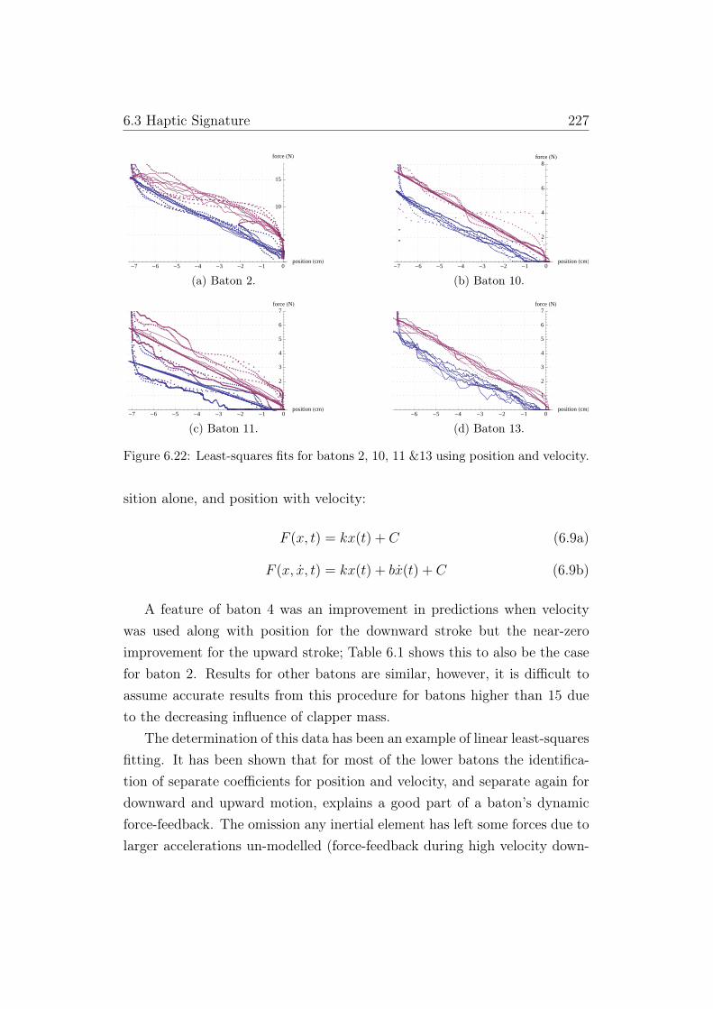
6.3 Haptic Signature 227
èèè
èèèèèèèèèèè
èèè
èèè
è
èè
è
èè
èè
èèèèè
èè
èèè è
èè
èè
è èè
èè
èè
èè
è è è è èè
èè
èè
èè
èè
èè
èè
èè
èè
èèè
èè
èè
è
è
è
è
èè
èè
èè
èè
è
è
è
è
è
è
èèèèèèèèèèè
èè
èè
èè
èè
èè
èè
èè è
è è èè
èè
èè
èè
èè
èè è è è
èè
è
è
è
è
è
è
è
è
è
è
èè
èè è è
èèè
èèèèèèèèèèèèèèèèèèèèèèèèèèèèèèèèèèèèèè
èèè
èèèèèèèè
èèè
è
è
è
è
è
è
è
è
è
èè
è èè è
èè
èè
èè
èè
èè
èè
è è è è è èè
èè
èè
èè
èè è è è è è
èè
èè
è
è
è
è
è
èèè
è
èèèè
èèèè
èèè
è
èè
è
èèèèèè
èèèèèè
èè
èèèèèèèè
èèèè
è èè
è èè
èèèè
èè
èè
èè
èè
è è èè è è è èè è
èè
è èèè
èèè
èè è
èèèèèèè
èèèèèèèèèèèèèèèèèèèèèèèèèèèè
èèè
è
è
è
èèèèèèè
èè
è
èè
èè
èè
èè
èè
èè
èè
èè
èè
è èè è
èè
èè
èè
èè
è
è
è
è
èè
è
è
èè
èè
èè
èè
èè
èè
èè
èèèèèèèèèèèèèèèèèèèèèèèèèèèèèèèèèèèèè
èèèèèèè
èèèèèè
èèèè
èèèèè
èèè
èè
èè
èè
èèè
èè
èè
èè
èè
èè
èè
èèè
èè
èèèèèèèèèèèèèèè
èè
èè
èè
èè
èè
èè
èè
èèèèèèèè
èè
è
èè
è
è
è
è
è
è
è
è
è
è
è
è
è
è
è
èè
èè
èè
èè
èèè
èèèèèèèèèèèèèèè
èèè
èèè
èèè
è
èè
èè
èè
èè
èè
èè
è
èè
è
è
è
èèè
èèèè
è
è
è
è
è
è
èè
èèè
èè
èè
èèèèèèèèèèèèèèèèèèèèèèèèè
è
è
è
è
è
è
è
è
è
è
è
è
è
èè
èè
èèèèèèèèèèèèèèèèèèèèèèèè
è
è
è
è
è
è
è
èè
èèèèèèèèèèèèèèèèèè
èèèè
èè
èè
èè
èè
èè
èè
èè
èè
èè
èèèè
èèè
èèèèèèèèèèèèèèèèèèèèèè
è
èè
è
èè
è
è
è
è
è
è
è
è
è
è
è
è
è
è
è
è
è
è
è
è
è
è
èè
èè
èèèèèèèèèèèèèèèèè
èè
è
è
èè
è
è
è
è
è
è
è
è
è
-7 -6 -5 -4 -3 -2 -1 0position HcmL
5
10
15
force HNL
(a) Baton 2.
èèèèèè
è
èè
è
è
è
è
è
è
èèè
è
è
è
è
è
è
è
è
èè
è
è
èè è è è è è
èè
èè
è
è
è
è
è
è
è
è
è
è
è
è
èè
èè è è è è
èè
èè
èè
è
è
è
è
è
è
èè è è è è è è è è è è è è èèèèèèèèèèèèèèèèèèèèèèèèèèèèèèèèèèè
è
è
è
è
è
è
èè
è
èè
è è
è
è
è
è
è
è
è
è
è
è
è
è
è
è
è
è
èè
è è è èè
èè
è
è
è
è
è
è
è
è èèèèèèèèèèèèèèèèèèèèèèèèèèèèè
è
è
è
è
è
è
è
è
èè
èè
èèèè
è
è
è
è
è
èè
è
è
è
è
èè è è è è
èè
èè
èè
èè
èè
èè
èè
èè
è
è
è
è
è
èè è è è è èèèèèèèèèèèèèèèèèèèèèèèèèèèèèèèèèèèèèèèèèèèèèèèèèèè
èè
è
è
è
è
è
è
è
è
è
è
è
è
èè
è
èèèèèèèèèè
èè
è
è
è
è
èè
èè
èè
èèèèèèèèèèèèèèè
èè
èè
èè
èè
èè
èèèèè
èè
èè
èèèèèèèèèèèèèèèèèèèèèèèèèèèèèèèèèèèèèèèèèèèèèèèèèèèè
èèèèèè
èèèèèèèè
èèèèèèèèèèèèèèèèèèèèèèèèèèèèèèèèèèèèèèèèèèèèèèèèèèèèèèèèèèèèèèèèèèèèèèèèèèèèèèèèèèèèèèèèèèèèèèèèèèèèèèèèèèèèèèè
èèèèèèèèèèèè
èèèèèèè
èèèèèèèèèèè
èèèèè
èèèèèèèèèèèèè
èèè
èè
èè
èè
èèè
èèè
èèèèèèè
èè
èè
èè
èèè
èè
è
è
è
è
è
èè
èè
èè
èèèèè
èèèèèèèèèèè
è
è
è
è
èèèè
èè
èèè
èè
èèèèè
èèèèèèèèèèèè
è
è
è
è
è
è
è
è
è
èè
èè
è
è
è
è
è
è
è
èè
èè
èè
èè
èè
è
è
è
è
è
è
èè
è
è
è
è
è
è
è
è
è
è
èè
èè
èè
è
èèèèè èè
è
è
è
è
è
è
è
è
èèèèèèèèè
è
è
è
èèè
èè
è
è
è
è
è
è
è
èèèèèèè èèèèèèèèèèèèèèèèèèèèèèèèèèèèèèèèèèèèèèèèèèèèèèèèèèèèèèèèèèèèèèèèèèèè
èèèèè
èèèèèèèèèèèèèèèèèèèèèèèèèèèèèèè
èèèè
èè
èè
èè
è
è
èè
èèèè
èè
èè
èè
èè
èèè
èè
èè
èèèè
èè
èè
èè
èè
èèèèèèè
èèèèèèèèèèèèèèèè
è
è
èèèèè
èèèè
èèèèèèèè
èèèèèè
èèèèèèèèèèèèèèèèèèèèèèèèèèèèèèèèèè
èèèèèèèèèèèèèèèèèèèèèèèèèèèèè
èèèèèèèèèèèèèèèèèèèèèèèèèèèèèèèèèèèèèèèèèèèèèèèèèèèèèèèèèèèèèèèèèèèèèèèèèèè
èèèèèè
èè
è
èè è
èè
èè
è
èè
èè
è è
è
è
è
è
è
èè
èè è è
èè
èè
è èè
èè
èè èè
èè
èè
èè
è è
èè
è
èè è
èè
è è è èèèèèè
èèèèèèèèèèèèèèèèèèèè
è
èè
èè
èè
è
è
èè
è è
è
è
è
è
è
è
è
èè
è
èè è
è
è
è
è
èè è
è
è
èè
èè è
èè
èèèèèèèèèèèèèè
èèèèè
èè
èè
èè
è
è
è
è
èè
è
è
èè
è
è
è è
è
è
è
è
è
èè
è
è
èè
èè
è è
è
è
è
èè
è
èè
è
èèèèèèèèèèèèèèèèèè
èèèèèèèèèèèèè
èèèèèèè
èè
èè
èèèèèèè
èè
èè
èèèèèèèè
èèèè
èèè
èèèè
èèèèè
èèèèèèèèèèèèèèèèèèèèèèèèèèèèèè
èèèèèèèèèèèèèèèèèè
èèèèèèèèè
èèèèèèèèèèèèèèèèèèèèèè
èè
èèèèèè
-7 -6 -5 -4 -3 -2 -1 0position HcmL
2
4
6
8force HNL
(b) Baton 10.
èèèèèèèèèèèèèèèèèèèèèèèèè
èèèèèèèè
èèè
è
è
è
è
è
è
è
è
èè
èè
èè
èè
èèèè è è è è
èè
èè
èè
èè è
èè
èè
èè
èè
èè è èèèè è è è è èèèèèèèèèèè
èèè
è
èèèèèèèèèèèèèèèèèèèèèèèèèèèèèèèèèèèèèèèèèèèèèèèèèèèèèèèèèèèèèèèèèèèèèèèèèèèèèèèèèèèèèèèèèèèèèèèèè
è
è
è
è
è
è
è
èèèèèèèèè
èè
è
è
è
èèèèèè
èè
èè
èèèèèè
èè
èè
èèèèèèèèèè
èè
èèèèèè
èèèèèèèèèèèèèèèèèèèèèèèèèèèèèèèèèèèèèèèèèèèèèèèèèèèèèèèèè
èèèèè
è
è
è
èèèèèèèèèèèèèèèèèèèèèèèèèèèèèèèèèèèèèèèèèèèèèè
è
è
è
è
è
è
è
è
è
èèèèèè
èè
èèèèè è è èè è
èè
èè
èè
èè è è è è è è è
èè
è
è
è
èè è è è è è èèèèèèè è èèèèèèèèèèèèèèèèèèèèè
è
è
è
è
è
è
è
è
è
è
è
èè
è è è è èè
èè è è è è è è è è è
èè
èè
èè
è
è
è
è
èè è è èèèèèè è èèèèèèèèèèèèèèèèèèèèèèèèèèèèèèèèèèèèèèèèèèèèèèèèèèèèèèèèèèè
è
è
è
è
è
è
è
è
è
è
èèèèèèèèèèèèèèèèèèèèèèèèèèèèè
èèèèèèèèèèèèèèèèèèèèè
èèèèèèèèèèèèèèèèèèèèèèèèèèèèèèèèèèèèèèèèèèèèèèèèèèèèèèèèèèèèèèèèèèèèèèèèèèèèèèèèèèèèèèèèèèèèèèèèèèèèèèèèèèèèèèèèèèèèèèèèèèèèèèèèèèèèèèèèèèèèèèèèèèèèèèèèèèèèèèèèèèèèèèèèèèèèèèèèèèè
èèèèèèèèèèè
èèèèèèèèèèè
èèèèèèèèèèèèèèèèèèèèèèèèèèèèèèèèèèèèèèèèèèèèèèèèèèèèèèèèèèèèèèèèèèèèèèèèèèèèèèèèèèèèèèèèèèèèèèèèèèèèèèèèèèèèèèèèèèèèèèèèèèèèèèèèèèèèèèèèèèèèèèèèèèèèèèèèèèèèèèèèèèèèèèèèèèèèèèèèèèèèèèèèèèèèèèèèèèèèèèèèèèèèèèèèèèèèèèèèèèèèèèèèèèèèèèèèèèèèèèèèèèèèèèèèèèèèèèèèèèè
èèèèèèèèèèèèè
èèèèèèèè
èèèèèèè
èèèèèè
èèèèè
èèè
èèè
èè
èè
èè
èè
èè
è
è
è
èè
èè
èèèèèèèèèè
èèèèèèèè
èèè
èè
èè
èè
èè
èèèè
èè
èèèèèèèè
èèèèèèèèèèèè
è
è
è
è
è
è
èèèèèèèèèèèèèèèèèèèèèèèèèè
è
è
è
è
èèèèè
èè
èèè
èèèèè
èè
èè
èè
èè
èè
èèèèèèèèè
èèèèèè
èè
èè
èèèèèè
èè
èè
èè
è
èè
èèèè
èèèèè
èèèè
èèèè
èèèèè
èèèèèèèèèèèèèèè
èèèèè
èèèèèèè
èèèèèèèè
èèèèèèèèèèè
èèèè
èè
èèèèèèèèèèèèèèèèèèèèèèèèè
è
è
è
è
è
èè
èè
èè
èèèèèèèèèèèèè
èè
èè
èèè
èèèèèèèèè
è
è
è
è
è
è
è
è
è
è
è
è
è
èèèèèèèè èèèèèè èèèèèèèè
è
è
è
è
è
è
è
è
è
è
èè
èè
è
è
è
è
èèè
èè
è
è
è
è
è
è
èèèèèèèèèè èèèèèèèèè èèèèèèèèèèèèèèèèèèèèèèèèèèèèèèèèèèèèèèèèèèèèèèèèèèèèèèèèèèèèèèèèèèèèèèèèèèèèèèèèèèèèèèèèèèèèèèèèèèèèèè
èèèè
èèèè
èè
èèè
èèèèèèèèèèèèèèèèèèèè
èèèèèèèèèèè
èèèèèèèèèèèèèèè
èèèèè
èèèèè
èèèèèèèèèèèèèèèèè
èèèèèèè
èèèèèèèè
èèè
èèèè
èèèèèèèè
èèèèèèèèèèèèèèèèè
èèèèèèèè
èèè
èèè
èèèè
èèèèèèèèèè
èèèèèèèèèèèèèèèè
èèèèèèèèèè
èèèèèèèèèè
èèèèèèèèèèèèèèèè
èèèèèèèèèèèèèèèè
èèèèèèèèèèèèèèèèè
èèèèèèèèèèèèèèèèèèè
è èèèèèèèèèèèèèèèèèèèèèèèèèèèèèèèè
-7 -6 -5 -4 -3 -2 -1 0position HcmL
1
2
3
4
5
6
7force HNL
(c) Baton 11.
èèèèèèèèèèèèèèèèèèèèèèèèèèèèèèèèèèèèèèèèèèèèèèèèèèèèèèèèèè
è
è
è
è
èè
è
èèè
èè
è
è
è
è
è
è
è
è
è
èè
èèè
èèè
èè
èè
èèèè
èè
èèèè
èèè
è
è
è
è
è
èè
è
è
è
è
è
è
èè
è
èè
èè è è è è è
èè
è è è èè
èè
èè
èè
èè è è è è è è è è è è è
è èè
èèè
èèèè
èè
èè
è
è
èè
èèè
èèè è è è èè è è è è è è è èèèèèèèèèèèèèèèèèèèèèèèèèèèèèèèèèèèèèèèèèèèèèèèèèèèèèèèèèèè
è
è
è
è
è
è
èèèèèèèèèèèè
èèèèèèèèèèèèèèèèèèèèèèèèèèèèè
èèèèèèèèèèèèèèèè
èèèè
èèèèèè
è
è
è
è
èèèèè
èè è è
è èèè èèèè
èè
èè
èèè
èèèèèèèèèèèèèèèèèèèèèèèèè
èèèèèèèèèèèèèèèèèèèèèèèèèèèèèèèèèèèèèèèèèèèèèèèèèèèèèèèèèèèèèèèèèèèèèèèèèèèèèèèèèèèèèèèèèèèèèèèèèèèèèèèèèè
èèèèèèèèèè
è
èèèèèèèèèèèèèèèèèèèèè
èèèèèèèèèèèèèèèèèèèèèèèèèèèèèèèèèèèèèèèèèèèèèèèèèèèèèèèèèèèèèèèèèèèèèèèèèèèèèèèèèèèèè
èèèèèè
èèèèè
è
èèèèè
è
è
è
è
è
è
è
è
è
è
èèèè
è
è
è
èè
èèèè
èèèèè
èè
è
è
è
è
è
è
è
èèè èèè è è è è
è
è
è
è
èè
èèèè è
èè
è
èè
èè
èè
èè è èè èèèèèèèè
èè
èèèèèèèèèèèèèèèèèè èèèèèèèè èè è è è è è è èè
èè
èè
èèèèèèèè
è
è
è
èè
èèèèèèèèèèèèèèèèèèèèèèèèèèèèèèèèèèèèèèèèèèèèèèèèèèèèèèèèèèèèèèèèèèèèèèèèèèèèèèèèèèèèèèèèèèèèèèèèèèèèèèèèèèèèèèèè
èè
èè
è
èè
èè
è
è
è
è
è
è
è
èèèèèè
èèèè
èè
èèèèèèè
èè
èè
èèèèèèèèè
èèèè
èèèèèèèèèèèèèèèèèèèèèèèèèèè
èèèèèèèèèèèèèèèèèèè
èèèèèèèèèèèè
èèè
èèèèèèè
èèèèèèè
èèèèèèèèèèèèèèèèèèèèèè
èèèèèèè
èèèèèèèèèèèèèèèèèèèèèèèèèèèèèèèèèèèèèèèèèèèèèèèèèèèèèèèèèèèèèèèèèèèèèè
èèèèèèèèèèèèèèèèèèèèèèèèèèèèèèèèèèèèèèèèèèèèèèèèèèèèèèèèèèèèèè
èèèèèèèèèèèèèèèèèèèè
èèèèèèèèèè
èèèèèèèèè
èèèèèèèè
èèèèèè
èèèèèèèèèèèèèèèèèèèèèèèèèèèèèèèèèèèèèèèèèèèèèèèèèèèèèèèèèèèèèèèèèèèèèèèèèèèèèèèèèèèèèèèèèèèèèèèèèèèèèèèèèèèèèèèèèèèèèèèèèèèèèèèèè
èè
è
èè
è
è
è
è
è
èè
èè
èè
èèèè
èèèèèè
èèèèèèèèèè
èèèè
èèèèèèè
èè
èèèè
èè
èè
è
è
è
èè
èè
èèè
èèèèèèèè
è
è
è
è
è
è
è
è
èè
èè
èè
èè
èè
èè
èè
èè
èè
èè
èè
èè
èèèèèèèè
èè
è
è
è
è
èè
èè
è
è
è
è
è
è
è
èèèèèèèèèèèèèèèèèèèè èèèèèèèèè
è
è
è
è
è
è
è
è
è
è
èè
èè
èè
èèè
èèèèèèèè
èè
èè
èè
èè
èè
èè
èè
èèè
èè
èè
è
è
è
è
è
è
è
è
è
èè
èèèèèèèèèèè
èè
èè
èè
èè
èè
èè
èè
èè
èè
èè
èè
èèèèèèèè
èè
èè
èè
è
èè
èè
èè
èèè
è
è
è
è
è
è
è
è
è
èè
èèè
è
è
è
èèèèèèèèèèèèèèèèèèèèèèèèèèèèèèèèèèèè
è
è
è
è
è
è
è
èè
èè
èè
èè
èè
èè
èè
èè
èèèèè
èè
è
è
è
è
è
è
è
èè
è
è
èè
èèèè
èè
èè
èè
èè
èè
èè
èè
èè
èè
èè
èè
èè
è
èè
èè
èèèè
èè
èèèèèèèèèèèè
èè
èè
èèè
è
è
è
èè
èèèè
èè
è
è
è
è
è
è
èèèèèèèè
èèèèèèèèèè
è
è
è
è
èè èèèèèèèèèèèèèèèèèèèèèèèèèèèèèèèèèèèèèèèèèèèèèèèèèèèèèèèèèèèèèèèèèèèèèèèèèèèèèèèèèèèèèèèèèèèèèèèèè
è
è
è
è
è
èè
èèèèèèè
èè
èè
èèèèèèèèèèè
èèè
èèèèèèèèèèèèèèèèèèèèèèèèèèèèèèèè
èèèè
èèèèèèèèèèèèèèèèèèèè
èèèèèèè
èèèè
èèèèè
èèèè
èèèè
èèèè
èèèè
èèèèè
èèè
èèèèèè
èèèè
èèè
èèèèèèèèèèèèèè
èèèèè
èèèèèèèèèèèè
èèè
èèèèèèè
èèèèèèèè
èèèè
èè
èèèèèèèèèèèèèèèèèèèèèèè
èè
èè
èèèèèè
èèè
èèèèèèèèèèèè
èèè
èèè
èèèèèèèèè
èè
èèèè
èè
èè
èèèè
èè
èèèèèèèèèèèèèè
èèè
è
è
èèèèèèè
èèèèèèèèèèèèèèèèèèèè
-6 -5 -4 -3 -2 -1 0position HcmL
1
2
3
4
5
6
7force HNL
(d) Baton 13.
Figure 6.22: Least-squares fits for batons 2, 10, 11 &13 using position and velocity.
sition alone, and position with velocity:
F (x, t) = kx(t) + C (6.9a)
F (x, x, t) = kx(t) + bx(t) + C (6.9b)
A feature of baton 4 was an improvement in predictions when velocitywas used along with position for the downward stroke but the near-zeroimprovement for the upward stroke; Table 6.1 shows this to also be the casefor baton 2. Results for other batons are similar, however, it is difficult toassume accurate results from this procedure for batons higher than 15 dueto the decreasing influence of clapper mass.
The determination of this data has been an example of linear least-squaresfitting. It has been shown that for most of the lower batons the identifica-tion of separate coefficients for position and velocity, and separate again fordownward and upward motion, explains a good part of a baton’s dynamicforce-feedback. The omission any inertial element has left some forces due tolarger accelerations un-modelled (force-feedback during high velocity down-

6.4 Baton Modelling with Wavelets 228
ward strokes is underestimated for batons 2, 4 and 10, for instance), but theseare accounted for when a mass is assigned to the particular model based onthe work in the previous section.
However, with baton 7 the limits of this type of linear analysis are ex-posed. A linear least-squares fit by definition minimises the least-squareserror of a linear fit; this means that a function with a conspicuous disconti-nuity is ‘averaged’ instead of modelled. This is certainly the case for baton 7.A plot of the position-only fit for baton 7 in Figure 6.23b demonstrates theeffect of this averaging: the detent between -3 and -4 cm is missed, and thediscontinuity requires that the fit mischaracterises the gradient both beforeand after this region. Inclusion of a velocity term in 6.23c does not improvethis — indeed, Table 6.1 shows no change in the R2 value for baton 7 withwhen velocity is also considered.
This suggests a nonlinearity or discontinuity in the force/position rela-tionship, and a nonlinear discrete wavelet model for force as a function ofposition and velocity is developed in the next section, alongside the linearleast-squares fit derived as for other batons in this section.
Summary
The haptic signature of several lower batons is presented and analysed, andusing linear fitting techniques haptic features for these batons are categorisedby their relationship to position and velocity. Force-feedback due to positionis roughly proportionate to position, and is roughly equal for downward andupward strokes.
6.4 Baton Modelling with Wavelets
The system identification literature offers several techniques for modellingnonlinearities in mechanical systems. They all, however, follow a basicschema: model a portion of the system as the sum of linear motion vari-ables and a constant, and then add some nonlinear function of position (usu-ally) and/or velocity (less usually). Suggested functions include polynomials,

6.4 Baton Modelling with Wavelets 229
3.5 cm�sec
-3.5 cm�sec
5 10 15 20force HNL
-6
-5
-4
-3
-2
-1
0
position HcmL
(a) Measured force/position.
èèèèè
è
èè
è
è
è
è
è
è
è
èè
èè
è
èè
è
è
è
è
èè
è è è è è è è è è èè
è
è
è
è
è
è
è
è
èè
èè è è
èè
è
è
è
èè
èè
èè
è
è
è
è
è
è
è
è
è
è
è
è
è
è
è
èè
è
è
è
è
è
è
è
èè è è è è è èèèèèèèèèèèèèèèèèèèèèèèèèèèèèèèèèèèèèèèèèèèèèèèèèèèèèèè
èè
è
è
è
è
è
è
è
è
è
è
è
è
è
è
èè
èè
èè
èè
èè
èè
èè
èè
è
è
è
è
è
è
è
èè
èè
èè
è è è è èè
èè
èè
èè
èè
èè
èè
èè
èè
èè
èè
èè
è
è
è
è
èè
èè
è èè
èè
è è è è è è è è èè
èè
è
è
è
è
èèèèèèèèèèèèèèèèèèèèèèèèèèèèèèèèèèèèèèèèèèèèèèèèèèèèèè
è
è
è
è
è
è
è
è
è
è
è
èè
èè
èèèèè è è è è è
èè
è
è
è
è
èè
èè
èè
èè
èè
èè
èè
èè
èè
èè
è
è
è
è
è
è
è
è
è
è
èè
èè
èè
èè
è
è
è
è
èè è èèèèèèèèèèèèèèèèèèèèèèèèèèè
è
èèèè
è
è
èèèèèèèèè
èèèèèèèè
è
è
è
è
è
è
è
è
è
èè
èè
èè
èè
èè
è è è è è è èè
è èè
èè
è
èè
èè
èè
èè
èè
èè
è
è
è
è
è
è
è
è
è
è
è
è
è
è
è
è
è
è
è
è
è
è
èè è èèèèèèèèèèèèèèèèèèèèèè
èèèèèèèèè
èè
è
è
èè
èèèè
èèèè
èèèè
èèèèèèèè
èèèèèè
èè
èè
èèèèèèèèèèè
èè èèèèè
èè èè
èè è è è è è è è è è èè
èè
èè è
è èèèè è è è
è èèè
èè
èè
èè
èèèèèèèèè
èè
èèèèèèèè è è èèèèèèèèèèèè èè
èè
èè
èè
èè
èè
èèèèèèèèè
èè
èè
èè
èè
è
è
è
èèèèèèèèèèèèèèèèèèèèèèèèèèèèèèèèèèèèèèèèèèèèèèèèèèèèèèèèèèèèèèèèèèèèèèèèèèèèèèèèèèèèèèèèèèèèèèèèèèèèèèèèèèè
èèè
èèèè
è
è
è
è
è
è
è
è
èèèèèèè
èèèèèèèèèèè
èèèèèèèèèèèèèèèèèèèèèèèèèèèèèèèèèèèèèèèèèèèèèèèèèèèèèèèèèèèèèèèèèèèèèèèèèèèèèèèèèèèèèèèèèèèèèèèèèèè
èèèèèèèèèèèèèèèèèè
èèè
èè
èè
èèèèèèèèèèèèèèèèèèèèèèèèè
èèèèèèè
èèèèèèèèèèèèèèèèèèèèèèèèèèèèèèèèèèèèèèèèèèèèèèèèèèèèèèèèèèèèèèèèèèèèèèèèèèèèèèèèèèèèèèè
èèè
è
è
è
è
èè
èè è è è è è è è è è è è è èèè
èèèèèèèèèèèèèèèèèèèèèèèèèèèèèèèèèèèèèèèèèèèèèèèèèèèèèè èèèèè
èèè
è
è
èèèèèèèèè
èèèèèè
èèèè
èè
èè
èè
è
è
è
è
è
è
è
èè
èè
èè
èè
èè
èè
èè
èè
èè
èè
èè
èè
èè
èè
èè
è
èè
èè
èè
èèèèè
èè
èè
èè
èèèèèèèèè
èè
èèèèèèèèè
èè
èè
èè
èè
èè
è
è
èè
èèèè
èè
èè
èè
èè
èèèèèèèèèèèèèèèèèèèèèèèè
è
è
è
è
èè
èè
èè
è
è
è
è
èè
èè
èè
èè
èè
è
èè
èè
èè
èè
èèè
èèèèèè
èè
è
è
è
è
èè
èè
èè
èèè
èèèè
èè
èè
èèè
èèè
èè
èè
èèèèè
èè
èèèèè
èè
èè
èè
èè
èè
èè
èè
èèèèèèèèè
èè
è
èè
è
è
è
è
è
è
è
è
è
è
èèèèèèèèèèèèèèèèèèèèèèèèèèèèèèèè
è
è
è
è
è
è
è
è
è
è
è
è
è
è
è
è
è
è
è
èè
èè
èè
èè
èèèè
èè
è
è
èè
èè
è
è
è
èè
èè
è
è
è
è
è
è
è
è
èè
èèè
èè
èè
èèèèèèèèè
èè
è
èè
èè
èèèè
èè
è
è
è
è
è
èèèèèèèèèèèèèèèèèèèèèèèèèèèèèèèèèèèèèèèè
è
è
è
è
è
è
è
è
è
è
è
è
è
è
è
è
è
è
è
è
èè
èè
èèè
èè
èè
èè
èè
èè
è
è
è
è
è
è
è
è
è
è
è
è
èè
èèèè
èèè
èèèè
èè
èèèè
èè
èè
èèè
è
è
è
è
è
èèèèèèèè
èè
èèèèèè èèèèèèèèèèèè
è
è
è
è
è
èè
èè
èè
èè
èè
èè
èè
èè
èè
èè
èè
èè
èè
èè
èè
è
èè
è
è
è
è
èè
èèè
èè
èè
èèèè
èèèèèèèè
èèè
èèèèèèèèèèèèèè
èè
èèè
èèèè
èèèèè
èè
èè
èèèèèèè
èèèè
èè
èèèèèèèèèèèèèèèèè
èè
èè
èè
èè
èèè
èè
èè
èèèèèèèèèèèèè
èè
èèèèèèèèèèèèèèèè
èè
èè
èèèèè
èè
èèèèèèèèèèèèèèèèèè
èèèèèèèèèèèèèèèèèè
èèèèèèèèèèèèèèèèèè èèèèèèèèèèèèèèèèèèèèèèèèèèèèèèèèèèèèèèèèèèèèèèèèèèèèèèèèèèèèè
è
è
è
è
èèèèè
èèèèè
èèèè
èèèèèèèè
èèèèèèèèèèèè
èè
èè
èèèèèèèèèèèèè
èèè
èè
èè
èèèèèèèèèèèèèèèèèè
èè
èèè
èèèèè
èèèèèèèèèèèèèèèèèèèè
èèèèèèèèèèèèè
èèèèèèèèè
èèèè
èèèèèèèèèèèèèèèèèèèèèèèèèèèèèèèèèèèèè
èè
èèèèèèè
èè
èè
èèèèèèèèèèèèèèèèèèè
èèè
èèèèèèè
èè
èèèèèèèèèèèèèèèèè
èè
èè
èèèèèèèèèèèèèè
èèè
èèèèèèè
èè
èè
èèèèèèè
èè
èèèèè
èèèè
èèèèèèèèèè
è
è
è
è
èèè
èèè
èèè
èèèè
èèèèèèèèèèèèèèèè èè
-6 -5 -4 -3 -2 -1position HcmL
2
4
6
8
10
12force HNL
(b) Position only.
èèèèè
è
èè
è
è
è
è
è
è
è
èè
èè
èè
èè
è
è
è
èè è è è è è è è è è è
èè
è
è
è
è
è
è
è
èè
èè è è
èè
è
è
è
èè
èè
èè
è
èè
è
è
è
è
è
èè
è
è
è
è
è
èè
è
è
è
è
è
è
è
èè è è è è è èèèèèèèèèèèèèèèèèèèèèèèèèèèèèèèèèèèèèèèèèèèèèèèèèèèèèèè
èè
è
è
è
è
è
è
è
è
è
è
è
è
èèèè
èè
èè
èè
èè è è è è
èè
è
è
è
è
è
è
è
èè
èè
èè
è è è è èè
èè
èè
èè
èè
èè
èè
èè
èè
èè
èè
èè
è
è
è
è
èè
èè
è èè
èè
è è è è è è è è èè
èè
è
è
è
è
èèèèèèèèèèèèèèèèèèèèèèèèèèèèèèèèèèèèèèèèèèèèèèèèèèèèèè
è
è
è
è
è
è
è
è
è
è
è
èè
èèèèèèè è è è è è
èè
è
è
è
è
èè
èè
èè
èè
èè
èè
èè
èè
èè
èè
è
è
è
è
è
è
è
è
è
è
èè
èè
èè
èè
è
è
è
è
èè è èèèèèèèèèèèèèèèèèèèèèèèèèèè
è
èèèè
è
è
èèèèèèèèè
èèèèèèèè
è
è
è
è
è
è
è
è
è
èè
èè
èèè è è è è è è è è è è
èè è
è
èè
è
èè
èè
èè
èè
èè
èè
è
è
è
è
è
è
è
è
è
è
è
è
è
è
è
è
è
è
è
è
è
è
èè è èèèèèèèèèèèèèèèèèèèèèè
èèèèèèèèè
èè
è
è
èè
èèèè
èèèè
èèèè
èèèèèèèè
èèèèèè
èè
èèèèèèèèèèèèèèè èè
èèèè
è èèèè è è è è è è è è è è
èè
èè
è èè èèè
è è è èè èè
èèè
èè
èè
èèèèèèèèèèèèèèèèèèè è è èèèèèèèèèèèè è
èè
èè
èè
èè
èè
èèèèèèèèèè
èè
èè è
èè
è
è
è
è
èèèèèèèèèèèèèèèèèèèèèèèèèèèèèèèèèèèèèèèèèèèèèèèèèèèèèèèèèèèèèèèèèèèèèèèèèèèèèèèèèèèèèèèèèèèèèèèèèèèèèèèèèèè
èèè
èèèè
è
è
è
è
è
è
è
è
èèèèèèè
èèèèèèèèèèè
èèèèèèèèèèèèèèèèèèèèèèèèèèèèèèèèèèèèèèèèèèèèèèèèèèèèèèèèèèèèèèèèèèèèèèèèèèèèèèèèèèèèèèèèèèèèèèèèèèè
èèèèèèèèèèèèèèèèèè
èèè
èè
èè
èèèèèèèèèèèèèèèèèèèèèèèèè
èèèèèèèèèèèèèèèèèèèèèèèèèèèèèèèèèèèèèèèèèèèèèèèèèèèèèèèèèèèèèèèèèèèèèèèèèèèèèèèèèèèèèèèèèèèèèè
èèè
è
è
è
è
èè
èè è è è è è è è è è è è è èèè
èèèèèèèèèèèèèèèèèèèèèèèèèèèèèèèèèèèèèèèèèèèèèèèèèèèèèè èèèèè
èèè
è
è
èèèèèèèèè
èèèèèè
èèèè
èè
èè
èè
è
è
è
è
è
è
èè
èè
èè
èè
èè
èè
èè
èè
èè
èè
èè
è
èè
èè
èè
èè
èè
èèè
èè
èèèèè
èè
èè
èè
èèèèèèèèè
èè
èèèèèèèèè
èè
èè
èè
èè
èè
è
è
èè
èèèè
èè
èè
èè
èè
èèèèèèèèèèèèèèèèèèèèèèèè
è
è
è
è
èè
èè
èè
è
è
è
èè
è
èè
èè
èè
èè
èè
èè
èè
èè
èè
èèèèèè
èèè
èè
è
è
è
èè
èè
èè
èèè
èèèè
èè
èè
èèè
èèè
èèèèèèèèèè
èè
èèèèè
èè
èè
èè
èè
èè
èè
èèèèèèèèè
èè
èè
èè
è
è
è
è
è
è
è
è
è
è
èèèèèèèèèèèèèèèèèèèèèèèèèèèèèèèè
è
è
è
è
è
è
è
è
è
è
è
è
è
è
è
è
è
è
è
èè
èè
èè
èè
èèèè
èè
è
è
èè
èè
è
è
è
èè
èè
è
è
è
è
è
è
è
è
èè
èèè
èè
èè
èèèèèèèèè
èè
è
èè
èè
èèèè
èè
è
è
è
è
è
èèèèèèèèèèèèèèèèèèèèèèèèèèèèèèèèèèèèèèèè
è
è
è
è
è
è
è
è
è
è
è
è
è
è
è
è
è
è
è
è
èè
èè
èèè
èè
èè
èè
èè
èè
è
è
è
è
è
è
è
è
èè
è
è
èè
èèèè
èèè
èèèè
èè
èèèè
èè
èè
èèè
è
è
è
è
è
èèèèèèèè
èè
èèèèèè èèèèèèèèèèèè
è
è
è
è
è
èè
èè
èè
èè
èè
èè
èè
èè
èè
èè
èè
èè
èè
èè
èè
è
èè
è
è
è
è
èè
èèè
èè
èè
èèèè
èèèèèèèè
èèè
èèèèèèèèèèèèè
èèè
èèè
èèèè
èèèèè
èè
èè
èèèèèèè
èèèè
èè
èèèèèèèèèèèèèèèèè
èè
èè
èè
èè
èèè
èè
èè
èèèèèèèèèèèèè
èè
èèèèèèèèèèèèèèèè
èè
èè
èèèèè
èè
èèèèèèèèèèèèèèèèèè
èèèèèèèèèèèèèèèèèè
èèèèèèèèèèèèèèèèèè èèèèèèèèèèèèèèèèèèèèèèèèèèèèèèèèèèèèèèèèèèèèèèèèèèèèèèèèèèèèè
è
è
è
è
èèèèè
èèèèè
èèèè
èèèèèèèèèèèèèèèèèèè
èè
èè
èèèèèèèèèèèèèè
èèè
èè
èè
èèèèèèèèèèèèèèèèèè
èè
èèè
èèèèè
èèèèèèèèèèèèèèèèèèèè
èèèèèèèèèèèèè
èèèèèèèèè
èèèè
èèèèèèèèèèèèèèèèèèèèèèèèèèèèèèèè
èèèèèèè
èèèèèèè
èè
èè
èèèèèèèèèèèèèèèèèèè
èèè
èèèèèèè
èè
èèèèèèèèèèèèèèèèè
èè
èè
èèèèèèèèèèèèèè
èèè
èèèèèèè
èè
èè
èèèèèèè
èè
èèèèè
èèèè
èèèèèèèèèè
è
è
è
è
èèè
èèèèèè
èèèè
èèèèèèèèèèèèèèèè èè
-6 -5 -4 -3 -2 -1 0position HcmL
2
4
6
8
10
12
force HNL
(c) Simple regression including velocity.
Figure 6.23: Force, position and velocity relationships, baton 7.
periodic functions like sinusoids or sawtooth, and wavelets.
6.4.1 The Wavelet Transform
The Discrete Wavelet Transform (DWT) is attractive because it represents afunction in both space and frequency;6 by design, it locates discontinuities,or differences, in a function. When analysing discontinuous or non-periodicfunctions this feature gives it an advantage over the Fourier transform, whichonly represents a function in the frequency domain. These differences are
6The DWT is usually referred to as a multiresolution time-frequency transform, howeverthe signals under consideration in this chapter are functions of position, not time, so theterm ‘space’ and ‘space-frequency’ is used.

6.4 Baton Modelling with Wavelets 230
stored in several layers of frequency resolution, called detail coefficients,which can be used to reconstruct the original function or some modifiedversion of that function; reconstruction is performed using the Inverse DWT(IDWT).
In order to spatially locate frequency features of a function, the Fouriertransform must be implemented using windowing (as in the short time Fouriertransform (STFT)). However, the SFTF is problematic because of its fixedwindow size and the uncertainty principle: a large fixed window sacrificesspacial localisation for greater frequency resolution, and a small fixed windowsacrifices frequency resolution for more accurate localisation.7
The wavelet transform automatically adjusts the size of the window tocompensate for high and low frequencies. As Miller and Colgate observe,this makes it suitable for modelling position-dependant force functions whichdepend on good position resolution [87]. The space-frequency grid for awavelet transform in Figure 6.24a illustrates these varying windows. Highfrequencies are recorded with better spatial resolution (small ∆x) but poorerfrequency resolution (large ∆f), and low frequencies are recorded with poorerspatial resolution but better frequency resolution (large ∆x and small ∆f).
These windows are created by translating (moving) and dilating (expand-ing/compressing) a mother wavelet ψ across a signal’s domain. These trans-lates and dilates are called wavelets, and are derived from the mother waveletby the relation in Eq. (6.10):
ψj,k(x) = 2j/2 ψ(2jx− k) (6.10)
Several translates and dilates are plotted for the Daubechies 8 mother wavelet(see [33]) in Figure 6.24b.
At each translation and dilation the inner product (notated as< f, ψj,k >)of the wavelet and the signal is calculated, and the result describes the weightor strength of that wavelet at that translation and dilation in the analysedsignal. These are the wavelet coefficients. The wavelet identity expresses the
7This is expressed in Gabor’s formula for describing the trade-off between frequencyand time resolution in acoustic quanta [48]: ∆t×∆f ≥ 1.

6.4 Baton Modelling with Wavelets 231
f∆x3 ∆x2
x∆x1∆x0
∆f 0
∆f 1
∆f 2
∆f 3
(a) Space-frequency grid for thewavelet transform.
-3 -2 -1 1 2 3x
-4
-2
2
4y
Daubechies 8 wavelet ΨHx, j,kL
(b) Daubechies 8 wavelet at dilations j ={21, 22, 23, 24} and translations k = {−4, 2, 14, 36}(left to right).
Figure 6.24: Daubechies wavelets and space-frequency representation of wavelettransform.
original signal as the sum of products of these coefficients with wavelets atappropriate translations and dilations:
f =∑j∈Z
∑k∈Z
< f, ψj,k > ψj,k (6.11)
The Discrete Wavelet Transform
The DWT decomposition theorem [14, p. 169] takes the wavelet identity andadds a scaling function φ; this scaling function forms the basis of a coarseapproximation of a signal upon which layers of wavelets describe increasinglevels of detail.
In a slight restatement of the wavelet identity: a signal f which can beapproximated by a scaling function fj at a sampling rate of 2j Hz can bedecomposed into an approximation component f0 and a series of waveletcomponents wl, where 0 ≤ l < j:
fj = wj−1 + wj−2 + . . .+ w0 + f0 (6.12)
An iterative decomposition algorithm (typically the Fast Wavelet Trans-

6.4 Baton Modelling with Wavelets 232
form, shown in Figure 6.25 below) produces a set of j detail coefficient vectors{blk} and one approximation coefficient vector a0k; the number of coefficientsk in each vector is determined by the number of resolution levels and thelength of the sampled signal.
f jH
L
2
2
b j-1
b j-2a j-1
H
L
2
2 a j-2 a 1b 0H
L
2
2 a 0
Figure 6.25: Wavelet decomposition by Fast Wavelet Transform (FWT). The sam-pled signal f j is passed through specially-related high and low pass filters (H andL) then downsampled to produce a detail vector bj−l which is stored, and an ap-proximation vector aj−l which is used for the next iteration until l = 0.
Using the following wavelet and scaling function expansions
wl =∑k∈Z
blkψ(2lx− k) for 0 ≤ l < j (6.13a)
f0 =∑k∈Z
a0kφ(x− k) (6.13b)
the coefficient vectors produced by the DWT can be plugged into the pre-vious Eq. (6.12) describing the composition of a function fj by wavelet andapproximation components. Any of these coefficients can be changed priorto recomposition in order to modulate the prevalence of frequency energyand arbitrary discontinuities in a recomposed signal.
This expansion can also be expressed in matrix notation for 1 ≤ n < N
force/position pairs and j detail layers, using only those translations kn thatare proximate to the point of interest xn:fj(xn)
...fj(xN)
=
b0ψ(20xn − kn) . . . bj−1ψ(2j−1xn − kn) a0φ(xn − kn)
......
......
b0ψ(20xN − kN) . . . bj−1ψ(2j−1xN − kN) a0φ(xN − kN)
1...1
(6.14)

6.4 Baton Modelling with Wavelets 233
Method
The following model takes advantage of two features of the wavelet transform:the identification of characteristic discontinuities and nonlinearities, and thesynthesis of arbitrary new functions that retain those characteristics. Thetransformed signal is force as a function of position, and the reconstructedsignal is modulated by velocity.
This section proceeds in the following steps:
1. Find a least-squares fit for a mass-spring-friction model with data fromrepeated downward and upward strokes for baton 7 (Figure 6.23a), andobserve that a nonlinearity related to position during the downwardstroke is left unmodelled.
2. Subtract forces associated with acceleration and velocity from the fit,leaving five functions (representing five separate downward strokes)comprised of the linear position and error components only. Collectthese functions and perform a DWT decomposition on their mean, re-sulting in a DWT with 7 vectors of wavelet coefficients that characterisefeatures common to each of the functions.
3. Show that any of the original functions can be reconstructed by scalarmultiplication of these base coefficient vectors, and that the magni-tude of those scalars is correlated with the velocity of the respectivefunctions.
4. Use this correlation to create a function that calculates a force outputfor a given position and velocity by multiplying the base coefficientswith velocity, then performing an Inverse DWT (IDWT).
6.4.2 Linear Least-Squares Fit
A least-squares estimate for the parameters {m,Cp, bp, Cn, bn, k, C} associ-ated with acceleration, positive and negative velocity (vp and vn), positionand a constant, is determined for baton 7 as modelled by a mass-spring-friction system with the non-stiction part of Karnopp friction. The observed

6.4 Baton Modelling with Wavelets 234
data for force, acceleration, velocity and position is contained in the vectorsFu, a,v and x.
Fu = ma + Cp sgn(vp) + bpvp + Cn sgn(vn) + bnvn + kx + C + ε (6.15)
3.5 cm�sec
-3.5 cm�sec
2 4 6 8force HNL
-7
-6
-5
-4
-3
-2
-1
position HcmLBaton 7 LLS fit
(a) Least-squares fit and observed data (dot-ted line).
1 2 3 4 5 6 7xHtL HcmL
-6
-4
-2
FHx,Ε,tL HNLFHx,Ε,tL
(b) Force due to position and error only.
Figure 6.26: Evaluation of LLS fit for baton 7.
This fit is then compared to the observed force/motion data and is seento miss an obvious nonlinearity: a mechanical detent halfway through thedownward stroke (Figure 6.26a). This nonlinearity appears to be related toposition, so the acceleration, velocity and constant terms are subtracted fromEq. (6.15) which leaves a function F (x, ε, t) that describes force at t due toposition x(t) and error ε(t) only:
F (x, ε, t) = kx(t) + ε(t) (6.16)
which is plotted in Figure 6.26b.
6.4.3 Force After Subtracting Velocity and Acceleration
This data is now re-arranged to describe force as a function of evenly-spacedposition steps rather than plotting a force value at time t against a position

6.4 Baton Modelling with Wavelets 235
value at t (Figure 6.27a); the functions are separated into five separate func-tions Fi. Velocity is also arranged as a function of evenly-spaced positionsteps, and plotted in Figure 6.27b.
20 40 60 80 100x HsamplesL
-7
-6
-5
-4
-3
-2
-1
F HNLFHxL
(a) The five functions Fi and their mean f(black line).
20 40 60 80 100x HsamplesL
-0.20
-0.15
-0.10
-0.05
v Hm�secLvHxL
(b) Velocity as a function of evenly-spacedposition steps.
Figure 6.27: Relationships between force, position and velocity, baton 7 data.Colours are matched between both figures, and for i = 1 . . . 5 are blue, red, yellow,green and orange.
These two plots suggest a relationship between the velocity and the‘smoothness’ of the five respective Fi functions: functions with higher ve-locities appear smoother than those with lower velocities. This is the firstindication that velocity may play a role in mediating the smoothness ofposition-related force for this baton, apart from the forces due to velocityalready accounted for by the Karnopp model.
The mean of the five functions, f , is calculated and shown as the blackline in Figure 6.27a. Here, f is calculated with each Fi equally weighted inorder to encapsulate characteristics from each Fi, however different weightsmay be used if particular characteristics of respective Fi are lost.

6.4 Baton Modelling with Wavelets 236
-4 -2 2 4
-0.5
0.5
Gaussian wavelet of derivative order 56
(a) Gaussian 56 wavelet for the CWT.
1 2 3 4 5 6 7
-1.0
-0.5
0.5
1.0Daubechies 8 wavelet and scaling function
(b) Daubechies 8 wavelet ψ and scaling func-tion φ (dashed), for the DWT.
Figure 6.28: Wavelets used for CWT and DWT.
6.4.4 Wavelet Transform (DWT and CWT) of Mean
Function
The mean function is transformed using the CWT (for visual analysis) andthe DWT. The wavelet used for the CWT is the Gaussian wavelet which iscreated by taking the nth derivative of the Gaussian function; here, the 56th
derivative is chosen, which places this mother wavelet in an appropriate fre-quency range for the analysed signal. After experimentation, the Daubechies8 mother wavelet was chosen for DWT analysis.
The wavelet scalogram (the CWT analog of the spectrogram for theFourier transform) in Figure 6.29a shows the continuous harmonic energylevels of f . Frequency energy in this figure is shown in the same way as thegrid in Figure 6.24a, with highest frequencies sampled at the finest resolutionat the top of the figure and lowest frequencies with the coarsest resolutionat the bottom.
Frequency ranges are grouped in octaves with 24 divisions to an octave;{6, 1}, for instance, represents frequency energy in the first 1/24th Hz of the6th octave. White gaps between blocks of dark colours indicate the absenceof energy in that octave at those locations.
Figure 6.29b shows the DWT multi-layer decomposition of f . This alsoillustrates energy levels at different refinements, however they are not repre-sented harmonically but in detail coefficient vectors {bj}60, and an approxima-

6.4 Baton Modelling with Wavelets 237
20 40 60 80 100x
810, 1<
89, 1<
88, 1<
87, 1<
86, 1<
85, 1<
84, 1<
83, 1<
82, 1<
81, 1<octaves
CWT of f HxL
(a) CWT
è è è è è è è è è è è è è è è
è è è è è èè è
è è
è
è
è
è è
èè è è è è è
è
è
è
è
è
è
è
è è
è è è è è èè
è
è
è èè
è
èè
èè
èè
è èè è è è
è
è
è
èè
è
è è èè
è
è
è
è èè
è èè
èè
èè
è
è
è
è
èè
è
è
è
è
èè
èè
èè è
è
è
èè
èè è è è è è è
è
è
è
è
èè è è è
è
è
è
è
è
èè
è
è
è
è
è
è
è
è
è
èè è è è è è è è è è è è è è è è è è è
è
è
è
è èè è è è è è è è è è è è è è è è
è èè
èè
è
èè
èè è è è
20 40 60 80 100x
b6
b5
b4
b3
b2
b1
b0
detail layersDWT of f HxL
(b) DWT
20 40 60 80 100x
w6
w5
w4
w3
w2
w1
w0
detail layersIn place IDWT of f HxL
(c) Individually resynthesised components ofDWT.
Figure 6.29: Continuous and discrete wavelet decompositions, baton 7. The bottomaxis in (b) and (c) is the approximation layer associated with the scaling functionthe DWT.
tion layer. The spacing of plot markers indicates that the detail layers rangefrom fine spatial resolution to coarse (descending from b6 to b0), with the finalapproximation layer containing a crude, almost linear approximation of thesignal. The finest layers are those captured as a highly-compressed wavelettraverses the signal, and the signal is leeched of information as the waveletexpands at each iteration until only the coarsest representation remains.
The wavelet components wi are plotted in Figure 6.29c. These are cal-culated from the coefficient vectors by the wavelet expansion Eq. (6.13a),and are shown here to relate coefficient vectors to the recomposition of theoriginal function.

6.4 Baton Modelling with Wavelets 238
6.4.5 Resynthesis of Original Functions
Does this set of detail and approximation coefficients contain enough infor-mation to synthesise any of the five original functions? At this point, it is notclear that it does. We wish to approximate any of the five original functionsFi by five new functions F ′i which are synthesised after multiplying the detailcoefficients {bjk} calculated for f with five coefficient vectors βi (leaving theapproximation coefficients unchanged).
Using the matrix representation of the wavelet expansion the problemis cast as finding a solution for the following linear system taken from Eq.(6.14) subject to the set of parameters βi:
F ′i (x1)
...F ′i (xn)
=
b0ψ(20x1 − k1) . . . bj−1ψ(2j−1x1 − k1) a0φ(x1 − k1)
......
......
b0ψ(20xn − kn) . . . bj−1ψ(2j−1xn − kn) a0φ(xn − kn)
βi0...
βij−1
1
Or, in wavelet component form, look to synthesise a new function F ′i thatresembles Fi by determining values for βi which minimise the square of theerror between the two functions over N data points:
F ′i (βi, x) = βij−1wj−1(x) + . . .+ βi0w0(x) + f0(x)
minβi∈R
N∑n=1
(F ′i (β
i, xn)− Fi(xn))2 (6.17)
Although linear least-square algorithms are typically faster than numericaloptimisation algorithms, numerical optimisation is able to take advantageof iterative recomposition algorithms like the FWT that are faster than thewavelet summations in Eq. (6.17). We use the Levenberg-Marquardt nu-merical optimisation algorithm, which is robust even when poorly initialised[104].
After numerical minimisation of Eq. (6.17), each of the five coefficientvectors βi are plotted along the horizontal in Figure 6.30a; the colours remaincoded to match the force and velocity plots in the earlier Figure 6.27 on page

6.4 Baton Modelling with Wavelets 239
è
è
èè
è
è
è
è
è
è
è
è
è
è
è
è
è
èè
è
è
è
è
è
è
è
è
è
è
è
è
è
è
è
è
è è è è è è è
Β0 Β1 Β2 Β3 Β4 Β5 Β6
-2
2
4
6
Β ji
(a) Detail multipliers for synthesis of the fiveoriginal functions, with mean β (black).
è
è
è
è
è
1 2 3 4 5Β
i
1.2
1.4
1.6
1.8
2.0
2.2
2.4
ΣI Β
iMStandard deviations HΣL of Β
i
(b) Coefficient multiplier standard devia-tions.
è
è
è
è
è
1 2 3 4 5Fi
-0.12
-0.10
-0.08
v-
m�sMean velocities Hvi
- L for original Fi
(c) Mean velocity of the five functions Fi.
Figure 6.30: Resynthesis coefficients and relation to mean velocities.
235. With that in mind, a visual inspection of the βi plots reveals that somesets of β have more variation than others; a comparison with Figure 6.27bwhich plots the velocity of each stroke against position hints at an inverserelationship between velocity and variation in β. The horizontal black linein Figure 6.30a represents the mean vector β of the set of multiplier vectors.
In fact, when the variation within each of the sets is expressed as standarddeviation it is very closely correlated with velocity associated with each of theoriginal functions, with a correlation coefficient of 0.97. Plotting the standarddeviation values alongside mean velocity visually confirms this (Figures 6.30band 6.30c).
Plotting the synthesised functions against the original functions in Figure6.31 shows that salient features of the original functions have survived theprocess. For instance, the roughness of F5, particularly in the second half

6.4 Baton Modelling with Wavelets 240
20 40 60 80 100x
-7
-6
-5
-4
-3
-2
-1
F HNLF¢
1
20 40 60 80 100x
-6
-5
-4
-3
-2
-1
F HNLF¢
2
20 40 60 80 100x
-6
-5
-4
-3
-2
-1
F HNLF¢
3
20 40 60 80 100x
-7
-6
-5
-4
-3
-2
-1
F HNLF¢
4
20 40 60 80 100x
-7
-6
-5
-4
-3
-2
-1
F HNLF¢
5
Figure 6.31: Synthesised functions F ′i (unbroken lines) approximating Fi (brokenlines).
of the x values, has been retained. The detent around x ≈ 50 has alsobeen retained for all functions despite being slightly different in character foreach function. It seems reasonable to work on the assumption that the baseDWT coefficients for f sufficiently characterise the observed position-relatedforce detents in Fi, and that simple scalar multiplication of each of the detailvectors is sufficient to approximate any of the original functions.
Fitting βi
While βi now contains a set of detail coefficient multipliers for each of theoriginal functions, it is helpful to make a further simplification if we aregoing to modulate a set of base detail coefficients with velocity: find somerelationship between these multipliers and the original functions’ velocities.
The mean of these detail coefficient multipliers, β, is fitted to each re-spective βi by multiplying it with a coefficient λi such that the square of the

6.4 Baton Modelling with Wavelets 241
error between a multiplier vector βi and λiβ is minimised:
minλi∈R
j−1∑l=0
(λiβl − βil
)2In this particular case, this has the effect of changing the height of the
black horizontal line to bring it as close as possible to the middle of the shapemade by each βi; the value of λi, then, is the scalar magnitude of deviationwithin any of the multiplier vectors. The estimated values for λi are plottedin Figure 6.32a.
è
è
è
è
è
1 2 3 4 5Β
i
0.5
1.0
1.5
2.0
Λ1
(a) Multipliers (λi) for βi.
ò
ò
ò
ò
ò
-0.12 -0.10 -0.08v
1.0
1.5
2.0
Λ
Λi as a function of vi
(b) Linear fit for λ as a function of meanvelocity v.
Again, this plot is similar in shape to the mean velocities in Figure 6.30c;the two variable sets have a correlation coefficient of 0.92.
A linear modelλ(v) = γ1v + γ0 (6.18)
with γ1 ≈ 20.8 and γ0 ≈ 3.1 describes the relationship quite well, with anR-squared value of 0.85.
6.4.6 Realtime Velocity Smoothing
With numerical values for the two parameters {γ1, γ0}, a linear function ofvelocity g(v, t) is defined as:
g(v, t,γ) = γ1v(t) + γ0 (6.19)
6.4 Baton Modelling with Wavelets 242
This equation is coupled with the wavelet expansion, so Eq. (6.13a) becomes
wl(x, v, t,γ) = g(v, t,γ)∑k∈Z
blkψ(2lx(t)− k) (6.20)
such that each detail coefficient layer is multiplied by the same velocity func-tion.
The velocity function g(v, t) can instead be included directly in the sumof wavelet components function Eq. (6.12):
fj(x, v, t,γ) = g(v, t,γ)
j−1∑l=0
wl(x, t) + f0(x, t) (6.21)
which is now a function that gives force feedback as a function of positionand velocity. Re-calculated at every time step t, this function is added tothe equation of motion for baton 7.
This function replaces the term for position in Eq. (6.15) in §6.4.2 so anequation of motion for baton 7 is now defined as:
F = mx+ Ffric(x) + fj(x, x,γ) + C (6.22)
with Ffric encapsulating the static and dynamic friction elements from theoriginal least-squares Eq. (6.15).
Even better values for γ1 and γ0 can be determined using those justestimated as initialisation values for an unconstrained minimisation of thefollowing function:
minγ∈R
T∑t=0
(Fu(t)− [mx+ Ffric(x) + fj(x, x,γ) + C])2 (6.23)
This procedure returns the estimates γ1 ≈ 15.7 and γ0 ≈ 2.1, and com-bining this updated wavelet function with the coefficients for acceleration,velocity and a constant we get a fit for baton 7 that captures the mechanicaldetent and the gradients before and after the detent (Figure 6.32).

6.4 Baton Modelling with Wavelets 243
3.5 cm�sec
-3.5 cm�sec
2 4 6force HNL
-7
-6
-5
-4
-3
-2
-1
position HcmLBaton 7 fit with wavelets
Figure 6.32: Resynthesised haptic profile for baton 7 with wavelet network.
6.4.7 Conclusion
Over the course of this chapter, a model has been developed for the hap-tic signature of the National Carillon, which includes static and dynamicforce-feedback. The change in force-feedback over the range of the caril-lon is associated with mechanical parameter changes which have now beenshown to be associated with previously widely-known properties of carillonbell manufacture and instrument design, endowing the model with significantpredictive properties.
An analysis of selected lower batons at low accelerations showed thatforce-feedback is linearly related to position and velocity, however in the caseof baton 7 a significant nonlinearity was observed. A Wavelet network wasdesigned which successfully modelled this nonlinearity in a process that canbe applied to arbitrary batons in foreign carillons..
Chapter 7
Haptic Model Validation
This previous chapter presented the behavioural characteristics of a carillonbaton: its haptic signature, and its signature motion. This chapter demon-strates that the haptic model developed over the the course of this thesissatisfactorily simulates the behaviour of the National Carillon.
Offline simulations are performed which show that the behaviour of thedynamic haptic model matches that of the real instrument under the twoconditions used in the previous chapter to illustrate signature motion: freemotion when released from the bottom of its stroke, and motion with anattached mass. The haptic signature is also simulated for low batons wheresuch data was collected. These simulation results demonstrate that the more-accurate cable-as-spring model is capable of emulating the full range of batonbehaviour, including idiosyncrasies associated with arbitrary kinematic anddynamic variations.
Evaluations with carillonneurs from the National Carillon are also con-ducted which show that the purpose-built haptic device described in Chapter5 is capable of simulating the haptic feedback of the real carillon to the sat-isfaction of performers across a wide range of skill levels and experience. Inthese evaluations, carillonneurs are asked to identify which baton on the realinstrument is being simulated by the haptic device, without any audio cuesfrom the device. Unlike the offline simulations, the haptic model used for thecarillonneur evaluations is the simplified linear model, developed alongside

7.1 Bell 4 Parameter Fitting and Validation 245
the cable-as-spring model in Chapter 4. Carillonneur validation of the gen-eral linear model, with no attempt to replicate idiosyncrasies associated withindividual batons, indicates that a foreign carillon might be sufficiently-wellemulated without requiring detailed dynamic data for each baton.
These two types of simulations are designed to validate the haptic modelacross the range of player interaction scenarios: when the player is not in con-tact with the baton the test is for it to move freely according to the dynamicsof that particular baton; when the player is in contact with the baton the testis for it to provide a combination of appropriate force-feedback and motiontoward and away from the carillonneur. From bell 20 up, the influence ofclapper mass and forward springs on the feel of the baton gives way to thereturn springs associated with lighter clappers. Modelling this change is keyto emulating the haptic signature of the entire instrument, which is experi-enced by the carillonneur as the progression from force-feedback associatedwith inertia and motion to force-feedback associated with stiffness.
Together, these offline simulations and user-evaluations demonstrate thatthe numerical parameters chosen for the model are accurate. For instance, thesignature motion of a low baton and a middle-range baton can be similar, butthe batons feel very different. The evaluations are also encouraging becausethe differences in static force-feedback for the highest 35 batons are veryminor, and the changing haptic sensation is mainly determined by the balancebetween clapper inertia and return springs. Positive results indicate thatthe dynamic model is capable of simulating these interactions in a realisticmanner for all batons, regardless of their mechanical differences.
7.1 Bell 4 Parameter Fitting and Validation
Over the course of this thesis a detailed model for bell 4 has been devel-oped, and many important parameters for that model have been measuredor calculated. However, some parameters, mostly relating to the behaviourof the clapper system, are yet to be determined. These include: energyloss due to clapper/damper and clapper/bell impact, energy loss due tobaton/damper impacts, a precise starting value and force constant for for-

7.1 Bell 4 Parameter Fitting and Validation 246
ward/return springs, and values relating to friction at several locations in thecarillon mechanism. Because most of these are related to clapper behaviour,this presents an opportunity to perform a validation of the mechanical andkinematic model.
The clapper system model is isolated, and its motion is fit recordingstaken of the real clapper system when disconnected from the crank; thisreturns values for the spring, damper impact and clapper friction. Withthese values in hand, the clapper model is ‘reconnected’ to the crank andbaton systems. Motion resulting from this configuration is then comparedwith that recorded at the baton. If these motions match, the crank andclapper models and the kinematic analyses of the linkages between all threesystems — that is, the complete carillon model — are validated.
7.1.1 Clapper Model Validation — Free Motion
The motion used to validate the isolated clapper is obtained by disconnectingthe clapper from the crank, and then pulling it up against the inside of thebell wall1 then releasing. The free motion that follows is recorded using aninertial sensor attached to the upper clapper rod.
One of the equations resulting from the dynamic models in the Chapter 4describes the equation of motion for the clapper itself, determined by solvingthe virtual-spring energy model for those potential and kinetic energies as-sociated only with the clapper, using the physical constants for bell 4 listedin Table 4.1 on page 131.
In order to simulate the clapper model using this equation, five parametersneed to be determined: starting value fmin and force constant ks for the returnspring; spring kd and impedance zd constants for the rubber damper, and africtional damping constant c. Of these we have rough measurements forthe spring start value and force constant (75N < fmin < 80N, and 250N/rad< ks < 350N/rad), and expect c to be a little less than zero. These rangesinform the initial value estimates supplied to the minimisation algorithm.
1Leaving a small gap to account for the distance during which the clapper is in freeflight and the baton is fully displaced.

7.1 Bell 4 Parameter Fitting and Validation 247
As in the previous chapter, the Levenberg-Marquardt minimisation algo-rithm is used because it performs well when a good initial guess cannot beprovided, as is the case with the rubber damper values. Again, the algorithmis implemented using the “NMinimize” function in Mathematica.
After minimising the squared-error between a simulated result and therecorded motion, the algorithm returns the following parameter values:
kd ≈ 65, 239N/m, zd ≈ 6860N/rad/sec
fmin ≈ 78N, ks ≈ −322N/rad
c ≈ −2.2N/rad/sec (7.1)
The recording and simulation results are shown in Figure 7.1.The simulated and recorded motion are agreeably similar, and the pa-
rameter values fmin and ks are within the expected range. There is, though,a discrepancy between the model and the data in the extent to which theclapper rebounds toward the bell wall after impact with the rubber damper.On the return after the first bounce the modelled clapper does not returnas far as the data, but is nicely aligned with the second, third and fourthbounces. Also, the sampled clapper compresses the damper further on thefirst impact despite being well-matched on the other impacts.
One of several explanations is that the spring component of the rubberdamper is modelled as a linear spring. The impedance term zd goes some wayto modelling a more complex restoration force although an examination ofthe two Figures 7.1a and 7.1b hints that the extent of compression is also non-linearly related to velocity. This is also suggested by the fact that althoughthe impact velocities in the latter plot decrease in a roughly linearly fashionthe depth of compressions in the former graph do not, with the second andthird impacts close to equal and the first impact significantly greater.
Another explanation for discrepancies between the model and the sampleddata is that the cable linking the lower clapper rod to the rubber damper isnot modelled, and could be introducing some backlash or spring effect.
Yet another possible explanation is that energy is lost to friction due

7.1 Bell 4 Parameter Fitting and Validation 248
0.5 1.0 1.5 2.0 2.5t HsecL
288.5
289.0
289.5
Θ1HtL °Simulated v. recorded clapper motion
Θ1min
recorded
simulated
(a) Rotational displacement over time.
0.5 1.0 1.5 2.0 2.5t HsecL
-0.10
-0.05
0.05
Θ1HtL°�secSimulated v. recorded clapper velocity
recorded
simulated
(b) Rotational velocity over time.
Figure 7.1: Bell 4 clapper model simulation against recorded data.
to lateral movement of the clapper during rotation. Although the clapperis firmly fixed at the revolute joint about the z-axis visible in Figure 7.2the clapper has been observed to wobble back and forth on its axis duringmotion. A likely source of this wobble is the complex reaction forces aboutthe pivot due to vibrations resulting from rubber damper impact, althoughnatural elements also play a part: wind coming off Lake Burley Griffin, forinstance. This motion causes non-linear friction at the revolute joint and atlow velocities may play a not-insignificant damping role; such wobble would
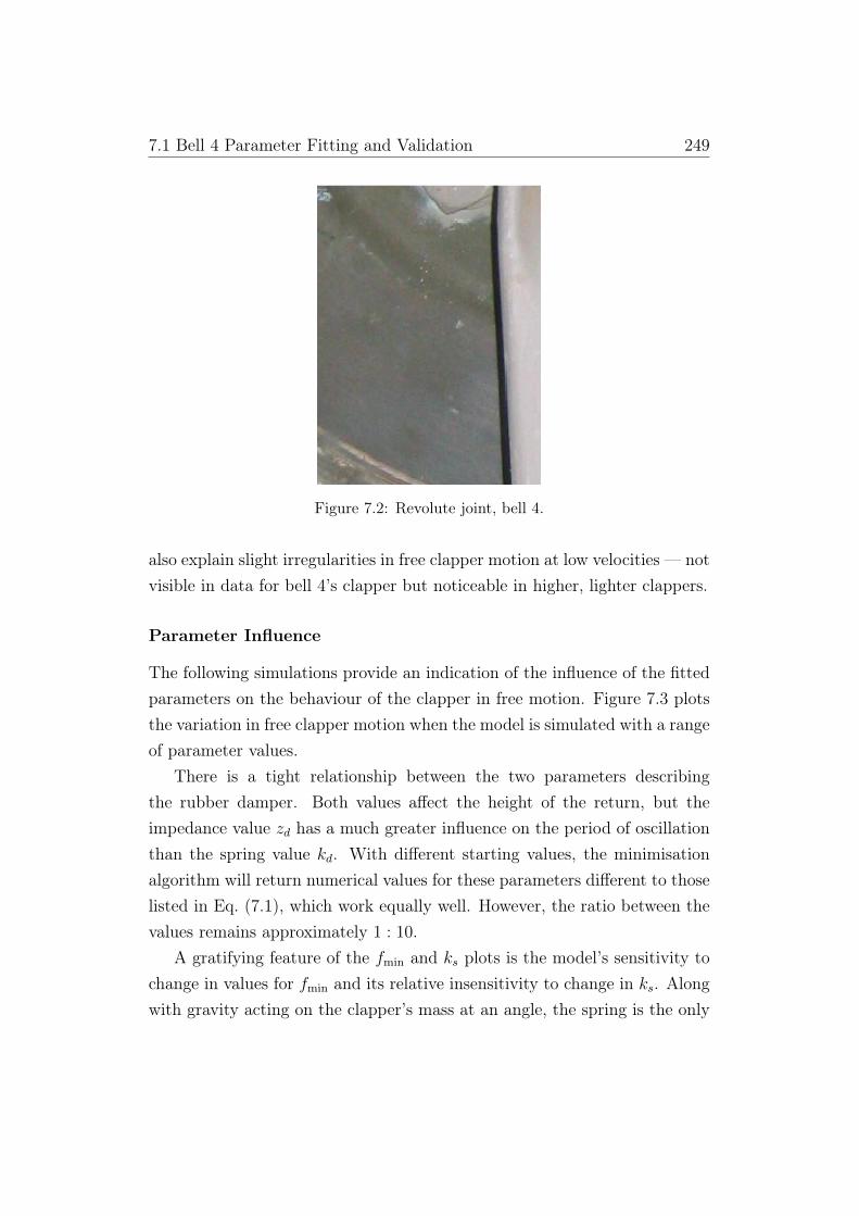
7.1 Bell 4 Parameter Fitting and Validation 249
Figure 7.2: Revolute joint, bell 4.
also explain slight irregularities in free clapper motion at low velocities — notvisible in data for bell 4’s clapper but noticeable in higher, lighter clappers.
Parameter Influence
The following simulations provide an indication of the influence of the fittedparameters on the behaviour of the clapper in free motion. Figure 7.3 plotsthe variation in free clapper motion when the model is simulated with a rangeof parameter values.
There is a tight relationship between the two parameters describingthe rubber damper. Both values affect the height of the return, but theimpedance value zd has a much greater influence on the period of oscillationthan the spring value kd. With different starting values, the minimisationalgorithm will return numerical values for these parameters different to thoselisted in Eq. (7.1), which work equally well. However, the ratio between thevalues remains approximately 1 : 10.
A gratifying feature of the fmin and ks plots is the model’s sensitivity tochange in values for fmin and its relative insensitivity to change in ks. Alongwith gravity acting on the clapper’s mass at an angle, the spring is the only

7.1 Bell 4 Parameter Fitting and Validation 250
kd - 30 000
kd - 15 000
kd + 30 000
kd + 80 000
0.5 1.0 1.5 2.0 2.5t HsecL
max
min
Θ1HtL °kd
(a)
zd - 3000
zd - 1500
zd + 1500
zd + 3000
0.5 1.0 1.5 2.0 2.5t HsecL
max
min
Θ1HtL °zd
(b)
fmin - 20
fmin - 10
fmin + 10
fmin + 20
0.5 1.0 1.5 2.0 2.5t HsecL
max
min
Θ1HtL °fmin
(c)
ks - 300
ks - 150
ks + 150
ks + 300
0.5 1.0 1.5 2.0 2.5t HsecL
max
min
Θ1HtL °ks
(d)
c � 0
c � -10
c � -25
c � -50
0.5 1.0 1.5 2.0 2.5t HsecL
max
min
Θ1HtL °c
(e)
Figure 7.3: Simulation results for changing fitted parameters, bell 4. The unbrokenline represents the recorded motion.
other contributor to torque about the clapper pivot, and therefore clappermotion when released from rest. The large variation in clapper motion inFigure 7.3c shows that the interaction between torque due to clapper massand angle, and torque due to the spring and clapper length is very finelybalanced indeed. An increase of 10 N in the spring starting value has theclapper travelling its entire range a full 100 msec later.

7.1 Bell 4 Parameter Fitting and Validation 251
The fact that the value for fmin is so close to the measured spring valueindicates that clapper parameters like mass, inertia and starting angle havebeen accurately determined in previous chapters. This is a particularly strongvalidation of the measurement and kinematic analysis of the linkage betweenthe crank and clapper, through which the clapper start angle is determined.
This model and the values in Eq. (7.1) are now carried into the fullyconnected model for verification.
7.1.2 Full Model Verification
Using the virtual spring model developed in §4.3, reconnecting the clapperto the crank system is simple. Instead of finding the equation of motion fromthe clapper potential and kinetic energy equations alone, those for the batonand crank system and the potential energy equations for the two linkingcables between the baton/crank and crank/clapper, are combined with theclapper equations. This is then solved for three time-dependant coordinates:the clapper, crank, and baton angles, θ1(t), θ2(t), and θ3(t) respectively. Thephysical models and constants used for the crank and baton systems are takenfrom the analyses presented in previous chapters of this thesis and includedin the full system model without alteration.
This full system is simulated from the same initial condition as for thelone clapper, with all coordinates at their maximum displacement. Motionresults from the simulation are shown in Figure 7.4. These plots only showthe first 0.5 seconds of motion in order to focus on the free motion priorto the first impact, which now involves collisions at two sites: the rubberdamper in the clapper system, and the felt-lined upper wooden beam in thebaton system.
The simulated clapper motion in Figure 7.4a matches very well with therecorded clapper motion; the baton motion results for the same simulationare shown in Figure 7.4b to match quite well with the recorded baton mo-tion, although the real baton is slightly quicker to rise than the simulation.Simulated crank motion is shown on its own in Figure 7.4c.
The motion simulated in the previous section for an isolated clapper is
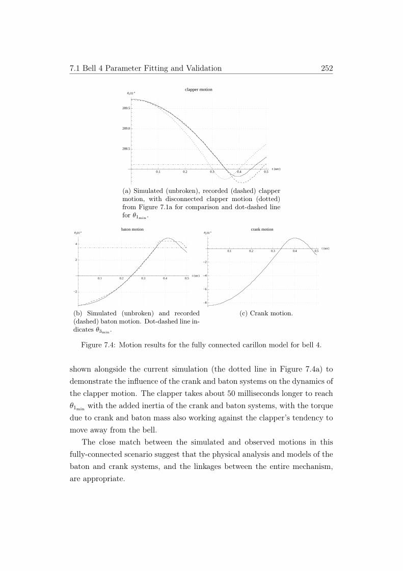
7.1 Bell 4 Parameter Fitting and Validation 252
0.1 0.2 0.3 0.4 0.5t HsecL
288.5
289.0
289.5
Θ1HtL °clapper motion
(a) Simulated (unbroken), recorded (dashed) clappermotion, with disconnected clapper motion (dotted)from Figure 7.1a for comparison and dot-dashed linefor θ1min .
0.1 0.2 0.3 0.4 0.5t HsecL
-2
2
4
Θ3HtL °baton motion
(b) Simulated (unbroken) and recorded(dashed) baton motion. Dot-dashed line in-dicates θ3min .
0.1 0.2 0.3 0.4 0.5t HsecL
-8
-6
-4
-2
Θ2HtL °crank motion
(c) Crank motion.
Figure 7.4: Motion results for the fully connected carillon model for bell 4.
shown alongside the current simulation (the dotted line in Figure 7.4a) todemonstrate the influence of the crank and baton systems on the dynamics ofthe clapper motion. The clapper takes about 50 milliseconds longer to reachθ1min with the added inertia of the crank and baton systems, with the torquedue to crank and baton mass also working against the clapper’s tendency tomove away from the bell.
The close match between the simulated and observed motions in thisfully-connected scenario suggest that the physical analysis and models of thebaton and crank systems, and the linkages between the entire mechanism,are appropriate.

7.1 Bell 4 Parameter Fitting and Validation 253
7.1.3 Full Model with Collisions
The model for the impact between the clapper and the rubber damper wasvalidated previously in §7.1.1. In this section both impact sites are includedand validated against recorded clapper and baton motion. The clavier im-pact is modelled in the same way as the rubber damper, but with differentconstants; these are determined by another round of parameter identification.
0.5 1.0 1.5 2.0 2.5t HsecL
-2
2
4
Θ3HtL °Baton motion
(a) Simulated (unbroken), recorded (dashed) batonmotion.
0.5 1.0 1.5 2.0 2.5t HsecL
288.5
289.0
289.5
Θ1HtL °Clapper motion
(b) Simulated (unbroken) and recorded(dashed) clapper motion.
0.5 1.0 1.5 2.0 2.5t HsecL
-8
-6
-4
-2
Θ2HtL °Crank motion
(c) Simulated crank motion.
Figure 7.5: Motion results for the fully connected carillon model for bell 4.
This simulation has the turnbuckle shortened by approximately 2mm.The slight jitter in the simulated baton motion is a product of the backlashintroduced by the turnbuckle and cable connection. This jitter can be reg-ulated by increasing or reducing the simulated cable stiffness. A value ofk1 = k2 = 105 N/rad is used for the simulations plotted in Figure 7.5; theplots in Figure 7.6 plots the simulation when the cable stiffness is increased to

7.1 Bell 4 Parameter Fitting and Validation 254
106 N/rad, removing backlash jitter but also failing to simulate the behaviourof the impact between the baton and the upper beam.
0.5 1.0 1.5 2.0 2.5t HsecL
-2
2
4
Θ3HtL °baton motion Hstiff cableL
(a) Simulation (unbroken) with parametersettings from simulation shown in Figure7.5.
0.5 1.0 1.5 2.0 2.5t HsecL
-2
2
4
Θ3HtL °baton motion Hstiff cable, re-calibrated upper beamL
(b) Simulation (unbroken) with alteredturnbuckle length and upper beam proper-ties.
Figure 7.6: Baton 4 with stiff cable (k1 = k2 = 106 N/rad) simulation. A stiffercable requires adjusted upper beam parameter values to match the recorded motion.
Simulation with Static Mass Attached
The model was also simulated with a static mass attached to the tip of thebaton; the results for this simulation are plotted in Figure 7.7. Whilst onlythe baton motion is compared to motion recorded at the carillon, motionfor the other systems is included to illustrate some of the consequences ofmodelling the cables as springs.
The simulated baton motion prior to impact with the bell and lowerwooden beam matches the recorded motion quite well. The recorded datacontains oscillatory jitter after impact, which is caused by the clapper andbaton systems becoming temporarily de-coupled as they impact with thebell and lower beam respectively. As they move independently, they cableconnecting the baton to the crank rapidly alternates between tautness andslackness. This behaviour is simulated by the model; although the oscillationsare not reproduced exactly, the general shape of the rebound is in goodagreement with the recording, and the shape of the early part of the reboundmatches closely until just after 0.4 sec.
The slackness in the cable at the very beginning of the cable is also
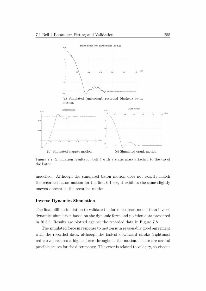
7.1 Bell 4 Parameter Fitting and Validation 255
0.2 0.4 0.6 0.8 1.0 1.2t HsecL
-4
-2
2
Θ3HtL °Baton motion with attached mass H2.5 KgL
(a) Simulated (unbroken), recorded (dashed) batonmotion.
0.2 0.4 0.6 0.8 1.0 1.2t HsecL
289.0
289.5
Θ1HtL °Clapper motion
(b) Simulated clapper motion.
0.2 0.4 0.6 0.8 1.0 1.2t HsecL
-8
-6
-4
-2
Θ2HtL °Crank motion
(c) Simulated crank motion.
Figure 7.7: Simulation results for bell 4 with a static mass attached to the tip ofthe baton.
modelled. Although the simulated baton motion does not exactly matchthe recorded baton motion for the first 0.1 sec, it exhibits the same slightlyuneven descent as the recorded motion.
Inverse Dynamics Simulation
The final offline simulation to validate the force-feedback model is an inversedynamics simulation based on the dynamic force and position data presentedin §6.3.3. Results are plotted against the recorded data in Figure 7.8.
The simulated force in response to motion is in reasonably good agreementwith the recorded data, although the fastest downward stroke (rightmostred curve) returns a higher force throughout the motion. There are severalpossible causes for the discrepancy. The error is related to velocity, so viscous

7.2 Offline Simulations 256
4.5 cm�sec
-4.5 cm�sec
5 10 15 20 25F HNL
-7
-6
-5
-4
-3
-2
-1
pos HcmLBaton 4
Figure 7.8: Inverse dynamics simulation (broken) and recorded data (unbrokenline).
damping that is modelled as proportional to velocity may be over-estimatedat some point in the model, or may be nonlinear greater than some thresholdvelocity.
7.2 Offline Simulations
The plots in Figures 7.14, 7.15, 7.16, and 7.17 printed at the end of thischapter show the results of offline simulations of the carillon model com-pared against recorded data for three scenarios, matching those describingthe carillon’s haptic signature: free motion after the baton has been heldat the bottom of its stroke; free motion with a static mass attached to thebaton tip, held at the top of its stroke and then released; and, dynamicforce-feedback in response to commanded motion, imitating the manner inwhich individual haptic signatures for low bells were recorded at the NationalCarillon.
Numerical parameters for these simulations were determined by a com-bination of initial estimates and manual tuning. The analysis of variation of
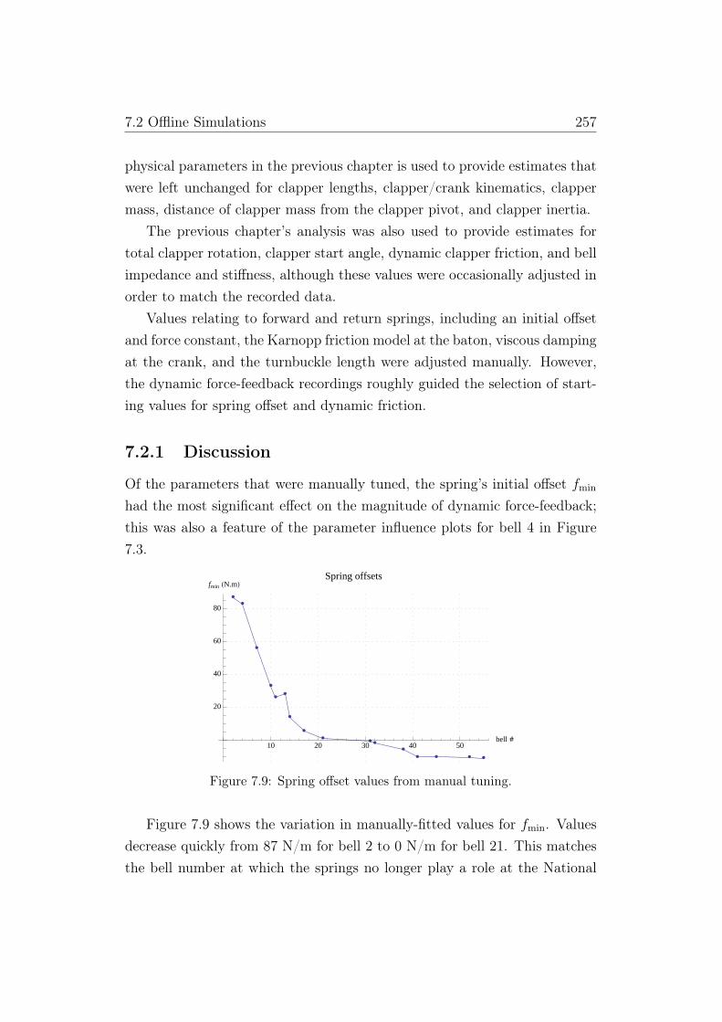
7.2 Offline Simulations 257
physical parameters in the previous chapter is used to provide estimates thatwere left unchanged for clapper lengths, clapper/crank kinematics, clappermass, distance of clapper mass from the clapper pivot, and clapper inertia.
The previous chapter’s analysis was also used to provide estimates fortotal clapper rotation, clapper start angle, dynamic clapper friction, and bellimpedance and stiffness, although these values were occasionally adjusted inorder to match the recorded data.
Values relating to forward and return springs, including an initial offsetand force constant, the Karnopp friction model at the baton, viscous dampingat the crank, and the turnbuckle length were adjusted manually. However,the dynamic force-feedback recordings roughly guided the selection of start-ing values for spring offset and dynamic friction.
7.2.1 Discussion
Of the parameters that were manually tuned, the spring’s initial offset fmin
had the most significant effect on the magnitude of dynamic force-feedback;this was also a feature of the parameter influence plots for bell 4 in Figure7.3.
è
è
è
è
èè
è
è
èè
è
è
è è è è
10 20 30 40 50bell #
20
40
60
80
fmin HN.mLSpring offsets
Figure 7.9: Spring offset values from manual tuning.
Figure 7.9 shows the variation in manually-fitted values for fmin. Valuesdecrease quickly from 87 N/m for bell 2 to 0 N/m for bell 21. This matchesthe bell number at which the springs no longer play a role at the National

7.3 Carillonneur Evaluations 258
Carillon. After bell 30, clappers feature return rather than forward springs,which are modelled simply as springs with negative force. By bell 40, thespring values are around -10 N/m, where they remain for the rest of therange.
The second most influential parameter was turnbuckle length. Thesevary arbitrarily across the simulations, depending on the turnbuckle settingwhen the motion data was originally connected. Adjustment of the virtualturnbuckle also proved a convenient way of replicating the dynamic effectsof components that would otherwise require more complex calculations, likethe clapper fly offset angle.
It is important to note of all the values that were fitted manually thatthey only recreate the motion and dynamic plots of the National Carillon atthe time when measurements were taken, and do not necessarily correspondto the physical values at the National Carillon at any other time.
7.3 Carillonneur Evaluations
In mid-2011, six carillonneurs who regularly rehearse and perform at theNational Carillon chose to take part in an evaluation of the haptic carillonbaton. The evaluations were conducted individually and consisted of a formalset of questions relating to experience, rehearsal and performance regimes, aninformal discussion regarding their thoughts on force-feedback in the carillon,a formal quantitative evaluation of the haptic baton simulating ten randombatons, and an informal discussion relating impressions of the haptic device.
7.3.1 Simplified Carillon Model
The linear mass-spring model developed alongside the cable-as-spring modelwas used to simulate baton motion and force-feedback for realtime evaluationby carillonneurs. Nonlinear Karnopp friction was included, as were positionconstraints imposed by a combination of the models for upper and lowerwooden beams at the baton, and bell wall and rubber damper at the clapper.
A separate continuous function was developed describing variation for
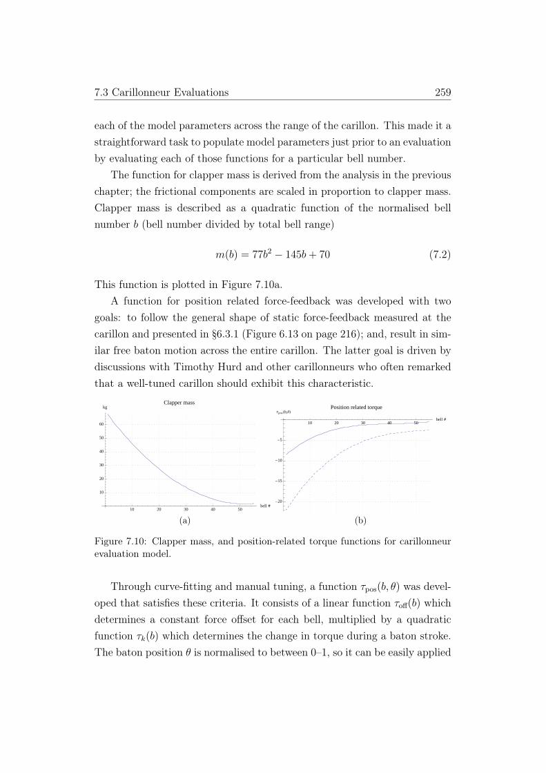
7.3 Carillonneur Evaluations 259
each of the model parameters across the range of the carillon. This made it astraightforward task to populate model parameters just prior to an evaluationby evaluating each of those functions for a particular bell number.
The function for clapper mass is derived from the analysis in the previouschapter; the frictional components are scaled in proportion to clapper mass.Clapper mass is described as a quadratic function of the normalised bellnumber b (bell number divided by total bell range)
m(b) = 77b2 − 145b+ 70 (7.2)
This function is plotted in Figure 7.10a.A function for position related force-feedback was developed with two
goals: to follow the general shape of static force-feedback measured at thecarillon and presented in §6.3.1 (Figure 6.13 on page 216); and, result in sim-ilar free baton motion across the entire carillon. The latter goal is driven bydiscussions with Timothy Hurd and other carillonneurs who often remarkedthat a well-tuned carillon should exhibit this characteristic.
10 20 30 40 50bell #
10
20
30
40
50
60
kgClapper mass
(a)
10 20 30 40 50bell #
-20
-15
-10
-5
ΤposHb,ΘLPosition related torque
(b)
Figure 7.10: Clapper mass, and position-related torque functions for carillonneurevaluation model.
Through curve-fitting and manual tuning, a function τpos(b, θ) was devel-oped that satisfies these criteria. It consists of a linear function τoff(b) whichdetermines a constant force offset for each bell, multiplied by a quadraticfunction τk(b) which determines the change in torque during a baton stroke.The baton position θ is normalised to between 0–1, so it can be easily applied

7.3 Carillonneur Evaluations 260
to sharp and natural batons alike.
τpos(b, θ) = τk(b)(τoff (b) + θ) + 2 (7.3a)
τoff(b) = 1.25b− 0.5 (7.3b)
τk(b) = −14b2 + 26b− 14 (7.3c)
This function is plotted in Figure 7.10b.Figure 7.11 shows the free motion plots for the simulated batons used in
carillonneur evaluations. The similarity in motion is quite clear, with staticfriction playing an increasing damping role in the motion of higher batons.
0.5 1.0 1.5 2.0 2.5t HsecL
-3
-2
-1
0
1
2
3
Θ3HtL °Baton simulations
(a) Batons 1, 5, 10, 20
0.5 1.0 1.5 2.0t HsecL
-3
-2
-1
0
1
2
3
Θ3HtL °Baton simulations
(b) Batons 30, 40, 50
Figure 7.11: Free motion simulation for simple model used in carillonneur evalua-tions.
7.3.2 Carillonneurs
All of the carillonneurs that participated in the evaluation perform on Na-tional Carillon regularly as part of the recital program, with a typical caril-lonneur performing twice a month, increasing to weekly during busy periods.
Their experience playing any carillon ranged from 5–47 years, with allhaving started on a different instrument, typically the piano or the organ.The more experienced carillonneurs tend to rehearse mainly on the real in-strument, with the most experienced carillonneur ‘virtually never’ rehearsingon the practice instrument. Other carillonneurs spend between 1–2/3rds of

7.3 Carillonneur Evaluations 261
their time on the practice instrument.All of the carillonneurs described the division of practice between the two
instruments in a similar way. The practice instrument was more likely to beused when preparing a new piece or figuring out an arrangement. When theyare in the final stages of preparing a piece for performance, they rehearse onthe real instrument. During this period, the carillonneur checks for timbraland harmonic problems arising from the complex bell tones that were notreproduced by the practice instrument; occasionally an arrangement will bere-written at this stage. Once a piece is fully prepared, the carillonneursdescribed rehearsing that piece exclusively on the real instrument in order tophysically condition themselves for the performance of that piece.
Informal Discussion
Prior to the evaluation of the haptic baton, each carillonneur was asked theirthoughts on the nature of force-feedback in the real carillon.
Almost all carillonneurs began their response by describing the practiceinstrument, which was universally considered ‘a totally separate instrument’,and its inadequacies. Many carillonneurs noted that was not possible to buildup the physical stamina required to perform the real instrument by rehearsingon the practice instrument alone. A few carillonneurs also described thepractice instrument as having a ‘harder’ feel than the real instrument. Thisis due to the fixed spring which accounts almost all the force-feedback fora practice baton, and provides no sense of inertia, so the entire practiceinstrument feels like the top few bells of the real instrument whose dynamicsare dominated by return springs.
Related to this, it was noted that the batons on the practice instrumentdo not stay in motion after a stroke like those on the real instrument. Thisparticularly irritated the less-experienced carillonneurs, some of whom de-scribed hurting themselves on the real instrument by failing to anticipatethat the baton was still in motion long after a previous strike.
Generally, carillonneurs were not particularly comfortable talking dis-cussing specific variation in force-feedback across the instrument apart from

7.3 Carillonneur Evaluations 262
the obvious increase in heaviness with low bells. There were some commentsregarding the motion of batons, with several carillonneurs emphasising theimportance of setting the turnbuckle lengths properly. In order to avoid set-ting up haptic cues that might influence responses in the formal part of theevaluation, these discussions were not pushed toward talking about differ-ent types of force-feedback across the instrument, or how it is related to thevariation in mechanisms.
7.3.3 Method
The haptic baton was programmed to randomly simulate 10 different batonsfor each of the six carillonneurs involved in the study. Each carillonneur wasassigned a set of batons spanning the instrument’s range, but the order inwhich the batons were simulated was randomised.
For each of the simulated batons, the carillonneur was asked to recordwhich of the real batons the haptic baton was simulating. They were freeto spend as much time as they liked on each simulation, and move betweenthe haptic baton and the real instrument. Whilst bell tones were audiblefrom the real instrument, sound was disabled on the haptic device in orderto ensure the carillonneur was relying only on their haptic and visual sensesduring estimation.
7.3.4 Results
The carillonneur estimates are plotted against the simulated batons in Figure7.12, where the unbroken line is the linear fit for their estimates and thebroken line is an ideal fit where a simulated carillon is estimated precisely.The mean error between estimated and simulated batons is -0.13 batons, andthe standard deviation in the error is 4.1 batons, approximately 1/3rd of anoctave.
This set of estimates omits the fourth, fifth, and sixth estimates madeby carillonneur 2, which were in error by a significantly greater margin thanthe rest of their estimates (see Figure 7.13b). These estimates were removed

7.3 Carillonneur Evaluations 263
è
è
è
è
è è
è
è
è è
è
è
è è
è
è
è
è
è
è
è
è
è
è
è
è
è
è
è
è
è
è
è
è
è
è
è
è
è
è
è
è
è
è
è
è
è
è
è
è
è
è
è
è
è
è
10 20 30 40 50simulated
10
20
30
40
50
estimatedEstimated and simulated batons
Figure 7.12: Carillonneur estimates plotted against the batons being simulated.The unbroken line is the linear fit y = 0.98x; the dashed line is y = x.
from consideration because the carillonneur themselves noted during the sim-ulation that they were unable to tell any of the middle-range batons aparton the real instrument, and recorded the estimates somewhat flippantly.
However, even with the inclusion of these estimates, the statistical out-come does not change significantly. The mean error increases to -0.5 batons,and the standard deviation in error increases to 4.5 batons.
The individual carillonneur estimates are plotted in Figure 7.13. Table7.1 lists the mean error and the standard deviation in error for the individualcarillonneurs.
7.3.5 Discussion
Carillonneurs tended to overestimate in the lowest 10 batons, recording amean error of 2.6 batons. This may point to a problem with the force-feedback model, but because carillonneurs rarely play low batons with theirfists, using foot-pedals instead, a lack of familiarity may have contributedto their reluctance to nominate these batons. Carillonneurs also tended tounderestimate the highest 10 bells, with a mean error of -1.4 batons. This
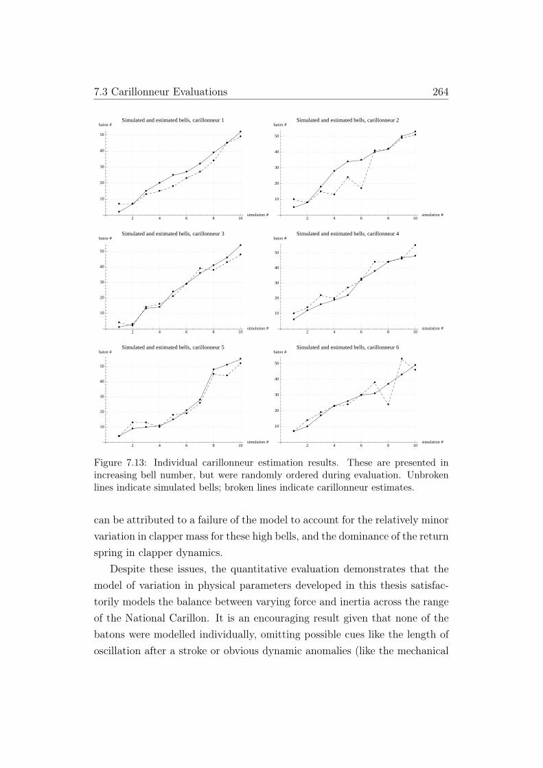
7.3 Carillonneur Evaluations 264
è
è
è
è
è
è
è
è
è
è
è è
è
è
è
è
è
è
è
è
2 4 6 8 10simulation #
10
20
30
40
50
baton #
Simulated and estimated bells, carillonneur 1
è
è
è
è
èè
è
è
è
è
è
è
è
è
è
è
èè
è
è
2 4 6 8 10simulation #
10
20
30
40
50
baton #
Simulated and estimated bells, carillonneur 2
è
è
èè
è
è
è
è
è
è
è
è
è
è
è
è
èè
è
è
2 4 6 8 10simulation #
10
20
30
40
50
baton #
Simulated and estimated bells, carillonneur 3
è
è
è
è
è
è
è
è
èè
è
è
è
è
è
è
è è
è
è
2 4 6 8 10simulation #
10
20
30
40
50
baton #
Simulated and estimated bells, carillonneur 4
è
èè
è
è
è
è
è
è
è
è
è è
è
èè
è
èè
è
2 4 6 8 10simulation #
10
20
30
40
50
baton #
Simulated and estimated bells, carillonneur 5
è
è
è
è
è
èè
è
è
è
è
è
è
èè
è
è
è
è
è
2 4 6 8 10simulation #
10
20
30
40
50
baton #
Simulated and estimated bells, carillonneur 6
Figure 7.13: Individual carillonneur estimation results. These are presented inincreasing bell number, but were randomly ordered during evaluation. Unbrokenlines indicate simulated bells; broken lines indicate carillonneur estimates.
can be attributed to a failure of the model to account for the relatively minorvariation in clapper mass for these high bells, and the dominance of the returnspring in clapper dynamics.
Despite these issues, the quantitative evaluation demonstrates that themodel of variation in physical parameters developed in this thesis satisfac-torily models the balance between varying force and inertia across the rangeof the National Carillon. It is an encouraging result given that none of thebatons were modelled individually, omitting possible cues like the length ofoscillation after a stroke or obvious dynamic anomalies (like the mechanical

7.3 Carillonneur Evaluations 265
Table 7.1: Carillonneur estimation results, mean error and standard deviation oferror, where error = estimated - simulated baton (* = with carilloneur 2 outliersremoved).
Carillonneur Mean Standard Deviation(batons) (batons)
1 -2.6 3.52 -4.3 72* 0 2.63 -0.7 34 2.9 3.15 -0.8 3.46 0.5 6.2All -0.5 4.5All* -0.13 4.1
detent in baton 7).It is also encouraging because the differences in static force-feedback for
the highest 35 batons are very minor (see static force feedback §6.3.1), andthe changing haptic sensation is mainly determined by the balance betweenclapper inertia and return springs. The positive results indicate that the dy-namic model is capable of simulating these interactions in a realistic mannerfor all batons, regardless of their mechanical differences.
Feedback After Evaluations
This is supported by informal feedback received during the evaluations. Inparticular, several carillonneurs remarked that they were confident of theirestimates because they had noticed during previous estimates that the devicereplicated the balance between the stiffness associated with return springs,and the inertial force associated with mass.
Several carillonneurs were surprised by the sensation of a return force pro-vided by the haptic baton. This was prevalent amongst the less-experiencedcarillonneurs, with comments like “I like the way it comes back up again”, and“[i]t returns home well”. All carillonneurs remarked on the heaviness of thehaptic baton when simulating a low bell, and seemed satisfied that a practice

7.3 Carillonneur Evaluations 266
instrument based on the haptic baton would be an appropriate substitute forthe real instrument for building up physical stamina.
However, after completing their ten evaluations, one of the carillonneursrequested that the baton be set to simulate the highest baton, 55. Theycompared this to the real instrument as well as the practice instrument, andremarked that the practice instrument felt closer to the real instrument thanthe haptic baton. After some discussion, it transpired that the carillonneurfelt the simulation was over-damped, and not returning with as firm a force asthe real instrument. The simulation was stopped, and the static friction andspring parameters manually adjusted, leaving virtual mass unchanged. Thesimulation was re-run with these adjusted parameters, and the carillonneurreported that it was a much better match.
Another carillonneur, after their evaluation, asked if the haptic batonspecifically modelled any of the idiosyncratic features of the National Caril-lon. They were answered in the negative, and it was explained that in thissimulation scenario the haptic baton aimed to evaluate the model of variationin force-feedback across the carillon rather than the dynamics of individualbatons. The carillonneur replied that this makes the haptic baton a usefultool for tuning carillons, and explained that they noticed several irregularchanges in force-feedback on the real instrument during the estimation pro-cess that they had missed during normal practice.
These two contrasting responses point to a range of possible applicationsfor a haptic carillon. The ease with which a manual parameter adjustmentcorrected the feel of a baton indicates that the dynamic model is sufficientlycomplex to emulate a variety of feels for a given clapper mass whilst not sotightly coupled that a change in one or two parameters requires re-adjustmentof others. The latter response indicates that a haptic carillon might play arole in synthesising and trialling force-feedback variation without physicaladjustments to a real instrument.

7.4 Summary 267
7.4 Summary
This chapter has presented a set of validations of the haptic carillon modeldeveloped over the course of this thesis. These validations are based on thedata presented as the haptic signature in the previous chapter.
Firstly, the mechanical analysis and the haptic model was validated bysimulating first the lone clapper motion, then the entire mechanism for bell 4.Dynamic force-feedback was also validated by performing an inverse dynam-ics simulation of bell 4 and comparing the force outputs to those recorded atthe real baton in response to the same motions.
Secondly, the analysis of variation in physical parameters across the Na-tional Carillon was validated when baton motion and dynamics across therange of the carillon was simulated, using numerical results from that analy-sis to populate the parameters of the dynamic model. Simulations spanningthe range of the carillon were conducted that showed the model matchingthe free motion and motion under static load, and dynamic motion for lowbells.
Finally, evaluations conducted with carillonneurs from the National Car-illon validated the haptic baton prototype, which encapsulates the controlsystem and sensing method developed in Chapter 5, the haptic model de-veloped in Chapter 4, and the analysis of variation in physical parameterspresented in Chapter 6. The quantitative evaluation demonstrated that themodelling captured the force-feedback of individual batons, and the changingnature of force-feedback across the range of the instrument. Informal feed-back also indicated that the haptic baton performed to a standard such thatan entire practice instrument constituting haptic batons would be superiorto existing practice instruments.

7.4 Summary 268
0.5 1.0 1.5 2.0 2.5 3.0t HsecL
-3
-2
-1
1
2
3
Θ3HtL °Baton 2
0.5 1.0 1.5 2.0t HsecL
-3
-2
-1
1
2
3
4
Θ3HtL °Baton 7
0.2 0.4 0.6 0.8 1.0 1.2t HsecL
-3
-2
-1
1
2
3
Θ3HtL °Baton 7 motion with attached mass H1.7 KgL
0.5 1.0 1.5 2.0 2.5t HsecL
-3
-2
-1
1
2
3
Θ3HtL °Baton 10
0.2 0.4 0.6 0.8 1.0 1.2t HsecL
-3
-2
-1
1
2
3
Θ3HtL °Baton 10 motion with attached mass H1.25 KgL
0.5 1.0 1.5 2.0 2.5 3.0t HsecL
-3
-2
-1
1
2
3
Θ3HtL °Baton 11
0.5 1.0 1.5 2.0 2.5 3.0t HsecL
-3
-2
-1
1
2
3
Θ3HtL °Baton 13
Figure 7.14: Low baton motion simulations (unbroken) against recorded motions(broken), free and with static mass attached.

7.4 Summary 269
3.5 cm�sec
-3.5 cm�sec
5 10 15 20 25 30F HNL
-7
-6
-5
-4
-3
-2
-1
0
pos HcmLBaton 2
3.5 cm�sec
-3.5 cm�sec
5 10 15 20 25 30F HNL
-7
-6
-5
-4
-3
-2
-1
0
pos HcmLBaton 7
6 cm�sec
-6 cm�sec
5 10 15 20F HNL
-7
-6
-5
-4
-3
-2
-1
0
pos HcmLBaton 10
6.5 cm�sec
-6.5 cm�sec
2 4 6 8 10 12 14F HNL
-6
-5
-4
-3
-2
-1
0
pos HcmLBaton 11
3 cm�sec
-3 cm�sec
2 4 6 8 10 12F HNL
-6
-5
-4
-3
-2
-1
pos HcmLBaton 13
Figure 7.15: Low baton inverse dynamics simulations.

7.4 Summary 270
0.5 1.0 1.5 2.0t HsecL
-3
-2
-1
1
2
3
Θ3HtL °Baton 21
0.2 0.4 0.6 0.8 1.0 1.2t HsecL
-4
-2
2
Θ3HtL °Baton 21 motion with attached mass H0.7 KgL
0.5 1.0 1.5 2.0t HsecL
-2
2
4
Θ3HtL °Baton 29
0.2 0.4 0.6 0.8 1.0 1.2t HsecL
-4
-3
-2
-1
1
2
3
Θ3HtL °Baton 29 motion with attached mass H0.42 KgL
0.5 1.0 1.5 2.0t HsecL
-3
-2
-1
1
2
3
Θ3HtL °Baton 30
0.2 0.4 0.6 0.8 1.0 1.2t HsecL
-3
-2
-1
1
2
3
Θ3HtL °Baton 30 motion with attached mass H0.42 KgL
Figure 7.16: Middle baton motion simulations (unbroken) against recorded motions(broken), free and with static mass attached.
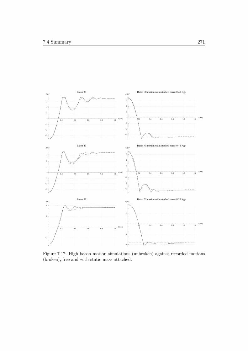
7.4 Summary 271
0.2 0.4 0.6 0.8 1.0t HsecL
-3
-2
-1
1
2
3
Θ3HtL °Baton 38
0.2 0.4 0.6 0.8 1.0 1.2t HsecL
-3
-2
-1
1
2
3
Θ3HtL °Baton 38 motion with attached mass H0.48 KgL
0.2 0.4 0.6 0.8 1.0t HsecL
-3
-2
-1
1
2
3
Θ3HtL °Baton 45
0.2 0.4 0.6 0.8 1.0 1.2t HsecL
-3
-2
-1
1
2
3
Θ3HtL °Baton 45 motion with attached mass H0.48 KgL
0.2 0.4 0.6 0.8 1.0t HsecL
-2
2
4
Θ3HtL °Baton 52
0.2 0.4 0.6 0.8 1.0 1.2t HsecL
-4
-2
2
Θ3HtL °Baton 52 motion with attached mass H0.28 KgL
Figure 7.17: High baton motion simulations (unbroken) against recorded motions(broken), free and with static mass attached.

Chapter 8
Conclusion and Future Work
8.1 Conclusion
8.1.1 The Carillon as a Public Instrument
The prototype haptic carillon developed in this thesis is designed to accom-modate the carillon’s unique status as a public instrument. Particularly out-side of North America, carillons are built and supported by local authorities,and fulfil several social functions ahead of their musical function. Moderncarillons continue to perform a public service in much the same way theyhave for the past five hundred years: marking the passing of time, augment-ing important social and religious events, alongside regular musical recitals.Modern carillonneurs also continue a tradition of mixed roles: every carillonhas the position of head carillonneur which is very much a public service andis maintained alongside any professional touring career the individual mayhave as a concert carillonneur. This creates an interesting and ever-presentdynamic between the carillonneur and their instrument; it is never reallytheir instrument, but rather permanently on loan.
Bell and carillon structures, particularly those built in modern times, arepublic monuments in themselves; the three carillons performed by membersof the Australian Carillon Society in Canberra, Sydney and Wellington (NewZealand), are officially the National Carillon, the War Memorial Carillon andthe National War Memorial Carillon [94]. This trend is not limited to the
8.1 Conclusion 273
antipodes: out of a total of the one-hundred and seventy-eight carillons inNorth America, one-hundred and twelve are either named after someone,memorialised to someone or their family [134].
Carillon performance schedules are another manifestation of the publicnature of the carillonneur’s art. In North America, carillons tend to markthe time with automated chimes, but feature regular (typically weekly) per-formances; carillons associated with academic institutions are also listed toperform at commencement and graduation ceremonies. The majority of car-illons attached to religious entities are performed at least several times aweek, typically augmenting an associated religious practice [134]. The Na-tional Carillon has thrice-weekly performances, increasing to each carillon-neur performing at least once a week during the summer months.
Heavy performance schedules in turn require significant amounts of reper-toire to be developed and mastered; the ability to rehearse in private is animportant factor in determining a carillonneur’s capacity to fulfil performanceduties.
Towards a Viable Rehearsal Instrument
As described in Chapter 1, almost all concert carillons feature a rehearsalinstrument along with the clavier for the actual instrument in the clavierroom. This rehearsal instrument will have the same physical dimensionsas the real clavier, but creates neither the acoustic feedback nor the hapticfeedback that a carillonneur can expect from a real instrument. The soundof the rehearsal instrument is typically generated by a felt-tipped hammer,connected to the vertical transmission rod by a revolute joint, which hits axylophone mounted within the keyboard frame. The touch of a rehearsalinstrument is typically generated by a helical spring connecting the verticalrod to the frame, providing a restoring force linearly related to the baton’sposition.
The literature on haptic interaction and motor skill acquisition reviewedin Chapter 2 justifies the efforts of 19th century carillonneurs like Jef Denynwho eschewed technological adaptations to the carillon mechanism which

8.1 Conclusion 274
removed the variation in force-feedback across the instrument. The exper-imental research also demonstrates the importance of reliable haptic cueswhen learning and refining physical gestures in scenarios that require preci-sion timing and efficient gesture execution; this research clearly supports thewidely-held perception that existing rehearsal instruments are largely ineffec-tual. A baton’s heaviness is a cue to the acoustic strength of its tone — theanalysis of baton keyfall and mechanical advantage between sharp and natu-ral keys in Chapter 3 illustrates how a modern carillon designer like TimothyHurd creates an acoustically-balanced instrument with careful mediation offorce-feedback.
The technological developments presented in this thesis towards a viablerehearsal instrument are founded in a respect for the efforts made by carillondesigners to present carillonneurs with an instrument capable of fulfilling themusical and cultural missions of the carillon.
8.1.2 Dynamic Models
A detailed mechanical model of the mechanism for bell 4 was presented inthe first half of Chapter 3. Each of the rotational systems were analysedindependently, and parametised equations describing dynamic and kinematicrelationships between them were developed that that allow the modellingof any other bell’s mechanism where accurate measurements can be taken.This accounts for the fact that physical characteristics of the mechanismvary across the range of the instrument. The final section of this chapterspecifically shows that many of the kinematic relationships can be modelledas linear equations; it ends by demonstrating that the variables in theseequations encapsulate physical properties, and are linearly related over therange of the instrument.
In Chapter 4 the mechanical model was used to develop two dynamic mod-els of bell 4; models for mechanical impacts between the baton and clavier,and the clapper and bell, were also developed. The first dynamic modelassumed uniform velocity between rotating systems based on fixed-length,massless rods connecting the systems; the model was linearised to yield a

8.1 Conclusion 275
second-order equation of motion for the baton, suitable for later system iden-tification and parameter fitting based on dynamic data collected at the baton.This generalised model accounts for inertia, friction and position-dependentforces which include springs and gravity acting on a clapper’s mass. Thisgeneralised model accounts for the dynamics of clappers without a preciseknowledge of their physical properties or kinematic arrangement. The seconddynamic model implemented the cables connecting rotating systems as stiffsprings that exert force only when expanded. This more accurate model iscapable of simulating the complex behaviour associated with linkage cableslosing tension during impacts, and the significant dynamic consequences ofslight changes in the turnbuckle length.
8.1.3 The Haptic Signature and Variation in Physical
Parameters
Haptic Signature
The deficiencies in the haptic feedback of rehearsal instruments are mostevident when considered in the context of a carillon’s haptic signature, de-veloped in Chapter 6. The haptic signature is designed along the lines ofWeir’s ‘haptic profile’ [129], and is expanded to include dynamic measure-ments of free motion and motion under static load, and the changing staticforce-feedback across the entire instrument. Unlike the haptic profile, a car-illon’s haptic signature is intended both as a data source for model fitting,and a conceptual aid for the consideration of haptic feedback across the in-strument.
Evidence of variation in haptic feedback is contained in the static force-feedback measurements taken across the instrument’s range. These show thevariation in static force required to hold the baton at different points in itsstroke, and that these forces do not exhibit much variation in bells 20–55.Variation in the haptic sensation in this range is dominated by changes inthe extent to which a clapper’s mass, and forward or return springs influencea baton’s dynamics.
Variation in the lower bells is determined by the dramatic changes in

8.1 Conclusion 276
clapper mass, with forward springs implemented specifically to mediate theincrease in force-feedback associated with gravity acting on these masses.Crucially, the forward springs do not shield the carillonneur from the inertiaassociated with the large masses for lower bells; the modern bell-crank mech-anism owes its popularity to the balance it provides between an appreciationfor the physical reality of the mechanism and ease of playability.
The haptic signature also gives an indication of the types of variation indynamic behaviour that develop in a carillon mechanism over time. Ideally,batons would exhibit similar free motion across the range of the instrument,with allowance for the massively greater inertia in low bells compared tohigher bells. The standard method of evaluating this similarity is to depressall the batons then release them at the same time: they should return andbounce at roughly the same rate. The data presented in Chapter 6 showsthat this was not the case during the period over which measurements foruse in this thesis were taken at the National Carillon; the free motion plotsshow significant variation between bells across the instrument’s range, andeven within narrow sets of neighbouring batons.
The dynamic force profiles, showing force as a function of position andvelocity during repeated downward and upward strokes for batons 1–15, alsodemonstrate a high degree of variation. These arise from the natural varia-tion in physical parameters, along with subtle and not-so-subtle mechanicaldefects or changes in configuration that occur over time.
Variation in Physical Parameters
These idiosyncrasies make it difficult to predict precisely the behaviour of anunknown carillon, however, the body of literature on the design of carillonbells provides a solid basis for predicting variation in physical parameters ofthe clapper across the range of a modern carillon.
In the first half of Chapter 6, statistical relationships were developedthat allowed the prediction of all clapper properties relevant to its dynamicbehaviour. The most important of these was the distance from the pointwhere the clapper is mounted to the ceiling of the bell to the point where it
8.1 Conclusion 277
is attached to a couple linking it to the crank. This property was stronglycorrelated with a bell’s height, which is itself predicted by its fundamentalfrequency according to the well-established literature and practice of carillonbell design. In turn, clapper length formed the basis of a model for predictingclapper mass and total clapper rotation. The length and rotation values areextended for use in predicting kinematic relationships between the clapperand crank at the end of Chapter 3.
Generalised Model Fitting
Using linear model fitting methods in Chapter 6, the generalised model withKarnopp friction was shown to satisfactorily simulate the dynamic force com-ponent of the haptic signature for several low bells. This indicates that therotational ranges of the heaviest bell’s clappers are small enough to be mod-elled as linear, therefore linearising the effect of gravity acting on clappermasses rotating about their pivots in the z-axis. These early validationsconfirmed the modelling approach thus far.
Modelling Mechanical Detents
However, the force profile for baton 7 showed a significant discontinuityaround halfway down the stroke. This was not unanticipated, as earlierdiscussions with carillonneurs had indicated that dealing with such defects isa regular part of carillon playing. Detailed analysis of the measured strokesrevealed a correlation between the velocity of a stroke and the smoothnessof the detent, with slower strokes experiencing larger detents.
This presented an opportunity to implement nonlinear modelling basedon the Discrete Wavelet Transform (DWT). A method was developed forthe realtime synthesise of a function describing force as a nonlinear func-tion of baton position, with baton velocity determining the smoothness ofthe function by modulating DWT coefficients. This approach yielded ex-cellent simulation results, but has not yet been perceptually evaluated —the mechanical detent was removed from the National Carillon in the periodbetween data collection and re-visiting for user-evaluations.
8.1 Conclusion 278
8.1.4 The Haptic Model
Chapter 5 described the design and construction of a prototype haptic deviceto evaluate the analytical work in the rest of this thesis. A key considera-tion was to design an interface that could easily be implemented in existingrehearsal carillons. A linear actuator was selected on the basis that it wouldbe a straightforward replacement for the helical springs currently used. Al-though this has not been tested in a rehearsal instrument, the prototype de-sign uses exactly the same parts as the rehearsal instrument at the NationalCarillon. This was demonstrated vividly when a part on the prototype failedduring user-evaluations, and Timothy Hurd was able to replace it directlyfrom the actual instrument.
On the basis of the literature reviewed in Chapter 2, an admittance con-trol scheme was chosen for controlling the actuator. This scheme was selectedfor its superior behaviour compared to an impedance control scheme when auser is not in contact with the baton. An admittance display requires someway of sensing carillonneur-applied force, and a sensor-less method based onobserving current commanded to an actuator from a position-control servocontroller was implemented. This noisy signal was filtered using a multi-sensor fusion technique based on the Kalman estimator, and system identifi-cation of the structure and parameters of the servo controller.
8.1.5 Validation
Finally, Chapter 7 presents a validation of the haptic model, and the com-putational models developed over the course of this thesis. This validationwas performed in two parts: offline simulations, and by user-evaluations.
Offline simulations were performed using the specialised models with acombination of predicted values based on bell scaling, and manually adjustedparameters relating to friction and spring force. These were evaluated againstrecorded motion, and were shown to be capable of generating the wide rangeof dynamic force and motion behaviours measured at the National Carillon.The intuitive nature of the dynamic model, based as it is on the actual mech-anism, suggests that this kind of parameter adjustment for individual batons
8.2 Future Work 279
could be performed by a carillonneur without the assistance of an engineer.In tuning the parameters for offline simulation, it was overwhelmingly theturnbuckle length and spring offset that determined the dynamic behaviourof the baton — both of these properties are well-known to carillonneurs.
The user-evaluations were performed using the generalised linear model,with inertia and friction parameters determined by the predicted values frombell scaling, and position-related force parameters automatically fit from thestatic force measurements. This model proved capable of simulating the mag-nitude and variation in haptic feel across the range of the National Carillon,even if it did not model idiosyncrasies particular to individual batons.
This result indicates that a linear dynamic model with parameters pop-ulated from predictive relationships and easily-obtained static force mea-surements at the baton is sufficient to satisfy the perceptual demands of apracticing carillonneur.
8.2 Future Work
The experimental results have shown that the linear dynamic model is capa-ble of simulating the haptic feedback of a relatively well-maintained carillon;these results form a basis upon which to evaluate the performance of themodel at older instruments that may be less well-maintained. In such in-struments, the additional degrees of freedom granted by the virtual springmodel may be utilised to replicate more complex behaviour. This thesis pre-sented an algorithm for augmenting the linear model with DWT synthesis;combining the DWT method with the virtual spring model to simulate thehaptic feedback of instruments that exhibit significantly deviant behaviouris a promising extension to this work. Such evaluations were not possible inthis thesis due to financial constraints associated with evaluations at othercarillons that might exhibit such behaviour. For the same reason, the nonlin-ear modelling method based on the DWT was not evaluated in a perceptualcontext.
Further evaluations would be aided by the development of a user-friendly,purpose-built device for measuring the haptic signature of a baton. Such a

8.2 Future Work 280
device would allow highly-automated model fitting, and facilitate the devel-opment of an international database of carillon dynamics, ready for simula-tion on an electro-mechanical rehearsal instrument. The algorithmic natureof the nonlinear modelling procedure developed in this thesis makes it suitedto automation with little user intervention.
Lastly, the haptic prototype was designed to be retrofitted to an existingrehearsal instrument. The sensor-less force-sensing method based on systemidentification and Kalman filtering developed in this thesis can be adaptedfor different actuator and control systems, as well as different mechanicalconfigurations. This opens the door to using several types of actuators andcontrollers within a single rehearsal instrument, making use of cheaper ormore readily-available hardware. The sensor-less force-sensing method canalso be used in other haptics applications which might otherwise be con-strained by a lack of appropriate force-sensors, particularly where the physi-cal region where the user interacts with the manipulandum is not limited toa single point.
Bibliography
[1] Richard J. Adams and Blake Hannaford. Stable Haptic Interactionswith Virtual Environments. IEEE Transactions on Robotics and Au-tomation, 15(3):465–474, 1999.
[2] Richard J. Adams, Manuel R. Moreyra, and Blake Hannaford. Stabilityand Performance of Haptic Displays: Theory and Experiments. InProceedings ASME International Mechanical Engineering Congress andExhibition, pages 227–34, 1998.
[3] Waskito Adi and Suziah Sulaiman. Haptic Texture Rendering Basedon Visual Texture Information: A Study to Achieve Realistic HapticTexture Rendering. In Halimah Badioze Zaman, Peter Robinson, MariaPetrou, Patrick Olivier, Heiko Schröder, and Timothy Shih, editors,Visual Informatics: Bridging Research and Practice, volume 5857 ofLecture Notes in Computer Science, pages 279–287. Springer Berlin /Heidelberg, 2009.
[4] Waskito Adi and Suziah Sulaiman. Using Wavelet Extraction for Hap-tic Texture Classification. In Proceedings of the 1st International VisualInformatics: Bridging Research and Practice, pages 314–325, 2009.
[5] Brian Armstrong and C. Canudas de Wit. Friction Modeling and Com-pensation. In William S. Levine, editor, The Control Handbook. CRCPress, 1996.
[6] H. Bagot. The Bell — Where Do We Stand Today? In Proceedings ofthe Fifth International Congress on Sound and Vibration, 1997.
BIBLIOGRAPHY 282
[7] James. A. Ballas. Self-produced Sound: Tightly Binding Haptics andAudio. In Haptic and Audio Interaction Design, pages 1–8, 2007.
[8] Tim Beamish, Karen Maclean, and Sidney Fels. Designing the HapticTurntable for Musical Control. In Proceedings of the 11th Symposiumon Haptic Interfaces for Virtual Environment and Teleoperator Systems(HAPTICS’03), pages 327–336, Vienna, Austria, 2003.
[9] E. Berdahl, G. Niemeyer, and J. O. Smith III. Using Haptics to AssistPerformers in Making Gestures to a Musical Instrument. In Proceedingsof New Interfaces for Musical Expression, 2009.
[10] E. Berdahl, B. Verplank, J. O. Smith, and G. Niemeyer. A Physically-Intuitive Haptic Drumstick. In Proceedings of the International Com-puter Music Conference, August 2007.
[11] Jonathan Berfer and Charles Nichols. Brahms at the Piano: An Analy-sis of Data from the Brahms Cylinder. Leonardo Music Journal, 4(23–30), 1994.
[12] A. L. Bigelow. The Acoustically Balanced Carillon. Princeton Univer-sity Press, 1961.
[13] David M. Birnbaum. Musical Vibrotactile Feedback. Master’s thesis,Schulich School of Music, McGill University, 2007.
[14] Albert Boggess and Francis J. Narcowich. A First Course in Waveletswith Fourier Analysis. Prentice-Hall, New Jersey, 2001.
[15] Florian Bömers. Wavelets in Real Time Digital Audio Processing:Analysis and Sample Implementations. Master’s thesis, University ofMannheim, 2000.
[16] Bert Bongers. The Use of Active Tactile and Force Feedback in TimbreControlling Musical Instruments. In Proceedings of International MusicConference, pages 171–174, 1994.

BIBLIOGRAPHY 283
[17] D. K. Brown. The Frictional Properties of Wool Felts. Wear, 6(1):22–29, 1963.
[18] Michael J. Brown and Edward J. Colgate. Passive Implementation ofMultibody Simulations for Haptic Display. In Proceedings of the 1997ASME International Mechanical Engineering Congress and Exhibition,pages 85–92, 1997.
[19] Michael J. Brown and Edward J. Colgate. Minimum Mass for HapticDisplay Simulations. In Proceedings of the 1998 ASME InternationalMechanical Engineering Congress and Exhibition, 1998.
[20] Claude Cadoz. Instrument Gesture and Musical Composition. In Pro-ceedings of the International Computer Music Conference, pages 1–12,1988.
[21] Claude Cadoz, A. Luciana, and Jean-Loup Florens. Responsive InputDevices and Sound Synthesis by Simulation of Instrumental Mecha-nisms: The Cordis System. Computer Music Journal, 8(3):60–73, 1984.
[22] Claude Cadoz, A. Luciana, and Jean-Loup Florens. CORDIS-ANIMA:A Modeling and Simulation System for Sound and Image Synthesis —The General Formalism. Computer Music Journal, 17(1):19–29, 1993.
[23] Craig R. Carignan and Kevin R. Cleary. Closed-loop Force Controlfor Haptic Simulation of Virtual Environments. Haptics-e, 1(2):1–14,2000.
[24] Chris Chafe. Tactile Audio Feedback. In Proceedings of InternationalMusic Conference, 1993.
[25] Manning Clark. A Short History of Australia. Penguin Books Australia,1986.
[26] Leszek Lisowski Claude Cadoz and Jean-Loup Florens. A ModularFeedback Keyboard Design. Computer Music Journal, 14(2):47–51,1990.

BIBLIOGRAPHY 284
[27] Albert Cohen and Jean-Pierre D’Ales. Nonlinear Approximation ofRandom Functions. SIAM Journal of Applied Mathematics.
[28] Edward J. Colgate and Michael J. Brown. Factors Affecting the Z-Width of a Haptic Display. In Proceedings of the IEEE 1994 Interna-tional Conference on Robotics and Automation, San Diego, CA., pages3205–3210, 1994.
[29] M. B. Colton and J. M. Hollerbach. Identification of Nonlinear PassiveDevices for Haptic Simulations. In WHC, pages 363–368, 2005.
[30] M. B. Colton and J. M. Hollerbach. Reality-Based Haptic Force Modelsof Buttons and Switches. In Proceedings of the 2007 IEEE InternationalConference on Robotics and Automation, pages 497–502, Roma, Italy,2007.
[31] Keyboard Committee. Consensus on Technical Norms for a WorldStandard Carillon Keyboard. Word Carillon Federation, 2006.
[32] Rod Cross. The Bounce of a Ball. The American Journal of Physics,67(3):222–227, 1998.
[33] Ingrid Daubechies. Ten Lectures on Wavelets. SIAM, 1992.
[34] Hanifa Dostmohamed and Vincent Hayward. Trajectory of ContactRegion on the Fingerpad Gives the Illusion of Haptic Shape. Experi-mental Brain Research, 164:387–394, 2005.
[35] J. Dunlop. Nonlinear Vibration Properties of Felt Pads. Journal of theAcoustical Society of America, 88(2):911–917, 1990.
[36] Sylvain Durand and Jacques Froment. Artifact Free Signal Denoisingwith Wavelets. In Proceedings of the 2001 International Conference onAcoustics, Speech and Signal Processing, 2001.
[37] Sylvain Durand and Jacques Froment. Reconstruction of Wavelet Co-efficients Using Total Variation Minimization. SIAM Journal on Sci-entific Computing, 24(5):1754–1767, 2003.

BIBLIOGRAPHY 285
[38] Randall L. Eubank. Spline Smoothing and Nonparametric Regression.New York: M. Dekker, 1988.
[39] Ernest Dean Fasse. On the Use and Representation of Sensory Infor-mation of the Arm by Robotics and Humans. PhD thesis, MassachusettsInstitute of Technology, 1992.
[40] Eric L. Faulring, Kevin M. Lynch, J. Edward Colgate, and Michael A.Peshkin. Haptic Display of Constrained Dynamic Systems via Admit-tance Displays. IEEE Transactions on Robotics, 23(1):101–111, 2007.
[41] The World Carillon Federation. Accessed: May, 2009http://www.carillon.org/.
[42] N. H. Fletcher, W. T. McGee, and A. Z. Tarnopolsky. Bell Clapper Im-pact Dynamics and the Voicing of a Carillon. Journal of the AcousticalSociety of America, 111(3):1437–1444, 2002.
[43] Neville Fletcher and Thomas Rossing. The Physics of Musical Instru-ments. New York: Springer, 1998.
[44] J.L. Florens. Expressive Bowing on a Virtual String Instrument:. InGesture-Based Communication in Human-Computer Interaction, Lec-ture Notes in Computer Science, pages 487–496. Springer Berlin / Hei-delberg, 2004.
[45] J. A. Florez and A. Velasquez. Calibration of Force Sensing Resistors(FSR) for Static and Dynamic Applications. In Proceedings of 2010IEEE ANDESCON, pages 1–6, 2010.
[46] A. Frisoli, M. Solazzi, F. Salsedo, and M. Bergamasco. A Finger-tip Haptic Display for Improving Curvature Discrimination. Presence,17(6):550–561, 2008.
[47] Shinichi Furuya and Hiroshi Kinoshita. Organization of the UpperLimb Movement for Piano Key-Depression Differs Between Expert Pi-anists and Novice Players. Journal of Experimental Brain Research,185:581–593, 2008.
BIBLIOGRAPHY 286
[48] Dennis Gabor. Acoustical Quanta and the Theory of Hearing. Nature,159(4044):591–594, 1947.
[49] Hong-Ye Gao. Wavelet Shrinkage Denoising Using the Non-NegativeGarrote. Journal of Computational and Graphical Statistics, 7(4):469–488, 1998.
[50] James M. Gere. Mechanics of Materials. Thomson, sixth edition, 2006.
[51] Sylvie Gibet and Jean-Loup Florens. Instrumental Gesture Modelingby Identification with Time-Varying Mechanical Models. In Proceedingsof 1990 International Music Conference, Köln, pages 28–40, 1990.
[52] Brent Gillespie. Dynamical Modeling of the Grand Piano Action. InProceedings of the International Computer Music Conference, 1992.
[53] Brent Gillespie. Haptic Display of Systems with Changing KinematicConstraints: The Virtual Piano Action. PhD thesis, Stanford Univer-sity, 1996.
[54] R. Brent Gillespie, Bo Yu, Robert Grijalva, and Shorya Awtar. Char-acterizing the Feel of the Piano Action. Computer Music Journal,35(1):43–57, 2011.
[55] Werner Goldsmith. Impact. Dover, 2001.
[56] John Gordon. Notes on the Art of Carillon Playing: A Guide forStudents. Number 3 in Sydney University War Memorial Carillon MusicSeries. Sydney: University of Sydney, 1939.
[57] John Gouwens. Playing the Carillon: An Introductory Method. TheGuild of Carillonneurs in North America, 2002.
[58] Mohinder S. Grewal and Angus P. Andrews. Kalman Filtering: Thoeryand Practice Using MATLAB. John Wiley & Songs, 2001.

BIBLIOGRAPHY 287
[59] Dong Guangbo, Xie Guihai, and Sun Zengqi. Real-time Audio De-noising DSP System Based on Wavelet Analysis and Pattern Recog-nition. In Proceedings of the International Conference on Neural Net-works and Brain, pages 826–830, 2005.
[60] D. Gugan. Inelastic Collision and the Hertz Theory of Impact. Amer-ican Journal of Physics, 68(10):920–924, 2000.
[61] Eric Gunther. Eric Gunther, Tactile Design. Accessed Januray, 2011http://www.ericgunther.info/tactile.html.
[62] Eric Gunther and Sile O’Modhrain. Cutaneous Grooves: Composingfor the Sense of Touch. Journal of New Music Research, 32(4):369–381,2003.
[63] Donald E. Hall and Anders Askenfelt. Piano String Excitation V: Spec-tra for Real Hammers and Strings. Journal of the Acoustical Society ofAmerica, 83(4):1627–1638, 1988.
[64] Rick S. Hall, Geoffrey T. Desmoulin, and Theodore E. Milner. A Tech-nique for Conditioning and Calibrating Force-sensing Resistors for Re-peatable and Reliable Measurement of Compressive Force. Journal ofBiomechanics, 41:3492–3495, 2008.
[65] Eiji Hayashi, Masami Yamane, and Hajime Mori. Behaviour of Piano-action in a Grand Piano. I. Analysis of the Motion of the HammerPrior to String Contact. Journal of the Acoustical Society of America,105(6):3534–3544, 1999.
[66] Vincent Hayward and Karen E. MacLean. Do It Yourself Haptics: PartI. IEEE Robotics and Automatic Magazine, 2007.
[67] Wilmar Hernández. Improving the Responses of Several AccelerometersUsed in a Car Under Performance Tests by Using Kalman Filtering.Sensors, 1:38–52, 2001.

BIBLIOGRAPHY 288
[68] William A. Hibbert. The Quantification of Strike Pitch and Pitch Shiftin Church Bells. PhD thesis, Faculty of Mathematica, Computing andTechnology, The Open University, 2008.
[69] M. C. Hirschkorn. Dynamic Model of a Piano Action Mechanism.Master’s thesis, University of Waterloo, 2004.
[70] Martin Hirschkorn, John McPhee, and Stephen Birkett. Dynamic Mod-eling and Experimental Testing of a Piano Action Mechanism. Journalof Computational and Nonlinear Dynamics, 1(1):47–55, 2006.
[71] G. Huang, D. Metaxas, and M. Govindaraj. Feel the "Fabric": AnAudio-Haptic Interface. In D. Breen and M. Lin, editors, Proceedings ofEurographics/SIGGRAPH Symposium on Computer Animation, 2003.
[72] Timothy Hurd. Chasing Creativity. Technical report, Carillon Societyof Australia, April 2008.
[73] Timothy Hurd. ‘WCF standard keyboard, baton lengths’. In emailconversation, 2010.
[74] Adel Izadbakhsh, John McPhee, and Stephen Birkett. Dynamic Mod-eling and Experimental Testing of a Piano Action Mechanism Witha Flexible Hammer Shank. Journal of Computational and NonlinearDynamics, 3(3):1–10, 2008.
[75] Matti Karjalainen, Paulo A. A. Esquef, and Vesa Välimäki. Making ofa Computer Carillon. In Proceedings of the Stockholm Music AcousticsConference, pages 1–4, 2003.
[76] Thorsten A. Kern, editor. Engineering Haptic Devices: A Beginner’sGuide for Engineers. Springer, 2009.
[77] Andre Lehr. A General Bell Formula. Acustica, 2:35–38, 1952.
[78] Andre Lehr. The Art of the Carillon in the Low Countries. Tielt(Belgium): Lannoo, 1991.

BIBLIOGRAPHY 289
[79] Sompong Lertpolpairoj, Thavida Maneewarn, Siam Charoenseang, andDjitt Laowattana. The Effect of Static Virtual Couplings on RealisticPerformance of Haptic Systems. In Asian Conference on Robotics andits Applications, pages 57–63, 2001.
[80] Shih-Tin Lin. Force Sensing Using Kalman Filtering Techniques forRobot Compliant Motion Control. Journal of Intelligent and RoboticSystems, 18:1–16, 1997.
[81] F.B. Llewellyn. Some Fundamental Properties of Transmission Sys-tems. Proceedings of the IRE, 40(3):271–283, 1952.
[82] Bing Lim Luk. Robot Force Sensing Using Stochastic Monitoring of theActuator Current. PhD thesis, Portsmouth Polytechnic, 1991.
[83] Yangyu Luo, Dangziao Wang, and Yuru Zhang. Stable Boundary ofVirtual Mass For a Haptic Admittance Display System. In Proceedingsof Eurohaptics, pages 242–252, 2003.
[84] Karen E. Maclean. The Haptic Camera: A Technique for Character-ising and Playing Back Haptic Properties of Real Environments. InProceedings of the International Mechanical Engineering Congress andExposition, 1996.
[85] Neil McLaclan and Densil Cabrera. Calculated Pitch Sensations forNew Musical Bell Designs. In Proceedings of the 7th InternationalConference on Music Perception and Cognition, Sydney, pages 600–603, 2002.
[86] Sebastian Merchel and Ercan M. Altinsoy. Vibratory and AcousticalFactors in Multimodal Reproduction of Concert DVDs. In Haptic andAudio Interaction Design, Lecture Notes in Computer Science, pages119–127, Berlin, Germany, 2009. Springer.
[87] Brian E. Miller and J. E. Colgate. Using a Wavelet Network to Char-acterize Real Environments for Haptic Display. In ASME InternationalMechanical Engineering Congress and Exposition, pages 257–264, 1998.
BIBLIOGRAPHY 290
[88] Brian E. Miller, J. Edward Colgate, and Randy A. Freeman. Guaran-teed Stability of Haptic Systems with Nonlinear Virtual Environments.IEE Transactions on Robotics and Automation, 16(6):712–719, 2000.
[89] Fazel Naghdy, Bing Lam Luk, and John Billingsley. Stochastic Com-pliance in a Robot-based Assembly. In Proceedings of InternationalConference on Control, pages 462–467, April 1988.
[90] Terumi Narushima. Composing for Carillon: Exploring the Relation-ship Between Tuning and Timbre. Master’s thesis, Sydney Conserva-torium of Music, University of Sydney, 2003.
[91] Tiffany Ng. The Development of the Organ and Carillon in the LowCountries to the Eighteenth Century. Unpublished Academic Paper,2006.
[92] Charles Nichols. The vBow: A Virtual Violin Bow Controller for Map-ping Gesture to Synthesis with Haptic Feedback. Organised SoundJournal, 7:215–220, 2002.
[93] Robert Oboe. A Multi-Instrument, Force-Feedback Keyboard. Com-puter Music Journal, 30(3):38–52, 2006.
[94] Carillon Society of Australia. Carillon Society of Australia.http://www.carillon.org.au/ Accessed: May, 2009.
[95] Allison M. Okamura, Matthew W. Hage, Mark R. Cutkosky, andJack Tigh Dennerlein. Improving Reality-Based Models for VibrationFeedback. Proceedings Haptic Interfaces for Virtual Environment andTeleoperator Systems Symposium, ASME, IMECE-2000, 69(2):1117–24, 2000.
[96] H. Olsson, K.J. Astrom, C. Canudas de Wit, M. Gafvert, andP. Lischinksly. Friction Models and Friction Compensastion. Euro-pean Journal of Control, 4(3):176–195, 1998.

BIBLIOGRAPHY 291
[97] Sile O’Modhrain. Playing by Feel: Incorporating Haptic Feedback intoComputer-Based Musical Instruments. PhD thesis, Stanford University,2000.
[98] Sile O’Modhrain. A Framework for the Evaluation of Digital MusicalInstruments. Computer Music Journal, 35(1):28–42, 2011.
[99] Sile O’Modhrain and Chris Chafe. The Performer-Instrument Interac-tion: a Sensory Motor Perspective. In Proceedings of the InternationalComputer Music Conference, Berlin, Germany, 2000.
[100] Dinesh K. Pai and L. M. Reissell. Haptic Interaction with Multireso-lution Image Curves. Computer and Graphics, 21:405–411, 1997.
[101] R. Perrin and T. Charnley. Normal Modes of the Modern EnglishChurch Bell. Journal of Sound and Vibration, 90:20–49, 1983.
[102] A. Pervozvanski and C. Canudas de Wit. Vibration Smoothingin Systems With Dynamic Friction. Technical report, Laboratoired’Automatique de Grenoble, 1997.
[103] Thao Tran Phuong, Chowarit Mitsantisuk, and Kiyoshi Ohishi. Multi-sensor Fusion in Kalman-filter for High Performance Force Sensing. InProceedings of the IEEE International Conference on Industrial Tech-nology (ICIT), pages 393–398, 2011.
[104] William H. Press, Saul A. Teukolsky, William T. Vetterling, andBrian P. Flannery. Numerical Recipes: The Art of Scientific Com-puting. Cambridge University Press, 3rd edition, 2007.
[105] Christopher Richard. On the Identification and Haptic Display of Fric-tion. PhD thesis, Stanford University, 2000.
[106] Louis B. Rosenberg and Bernard D. Adelstein. Perceptual Decomposi-tion of Virtual Haptic Surfaces. In Proceedings of IEEE 1993 Sympo-sium on Research Frontiers in Virtual Reality, San Jose, CA., 1993.

BIBLIOGRAPHY 292
[107] Thomas D. Rossing and Robert Perrin. Vibrations of Bells. AppliedAcoustics, 20:41–70, 1987.
[108] Joseph Rovan and Vincent Hayward. Typology of Tactile Soundsand Their Synthesis in Gesture-Driven Computer Music Performance,pages 297–320. IRCAM, 2000.
[109] Leonid I. Rudin, Stanley Osher, and Emad Fatemi. Nonlinear TotalVariation Based Noise Removal Algorithms. Physica D, 60(259–268),1992.
[110] D. Russell and T. Rossing. Testing the Nonlinearity of Piano HammersUsing Residual Shock Spectra. Acustica, 84(5):967–975, 1998.
[111] Gary Scavone and Andrey da Silva. Frequency Content of BreathPressure and Implications for Use in Control. In Proceedings of the2005 Conference on New Interfaces for Musical Expression (NIME-05), 2005.
[112] Richard A. Schmidt and Timothy D. Lee. Motor Control and Learning:A Behavioral Emphasis - 4th Edition. Human Kinetics Publishers,2005.
[113] S. Serafin, C. Vergez, and X. Rodet. Friction and Application to Real-time Physical Modeling of a Violin. In Proceedings of InternationalMusic Conference, pages 216–219, 1999.
[114] T. Shimono, S. Katsura, and K. Ohnishi. Haptic Motion Control forPhysical Human Support. IEEJ Transactions on Electrical and Elec-tronic Engineering, 4:166–175, 2009.
[115] Eugen Skudrzyk. Simple and Complex Vibratory Systems. Pennsylva-nia State University Press, University Park, PA, 1968.
[116] Nontapol Somrang and Nopporn Chotikakamthorn. Interactive HapticSimulation of Dental Plaque Removal. In International Symposium onCommunication and Information Technology, pages 319–322, 2006.
BIBLIOGRAPHY 293
[117] Colin Swindells and Karen E. MacLean. Capturing the Dynamics ofMechanical Knobs. In WHC ’07: Proceedings of the Second Joint Eu-roHaptics Conference and Symposium on Haptic Interfaces for VirtualEnvironment and Teleoperator Systems, pages 194–199, Washington,DC, USA, 2007. IEEE Computer Society.
[118] Yoshiyuki Tanaka, Tatsuya Abe, Toshio Tsuji, and Hideki Miyaguchi.Motion Dependence of Impedance Perception Ability in Human Move-ments. In Proceedings of the First International Conference on ComplexMedical Engineering, 2005.
[119] P. M. Taylor and D. M. Pollet. Low-Force Dynamic Lateral Compres-sion of Fabrics. Textile Research Journal, 72(10):845–853, 2002.
[120] Toshio Tsuji, Yusaku Takeda, and Yoshiyuki Tanaka. Analysis of Me-chanical Impedance in Human Arm Movements Using a Virtual TennisSystem. Journal of Biological Cybernetics, 91:295–305, 2004.
[121] E. W. van Heuven. Acoustical Measurements of Church Bells and Car-illons. De Gebroeders van Cleef, Hague, 1949.
[122] Bill Verplank, Michael Gurevich, and Max Mathews. The Plank: De-signing a Simple Haptic Controller. In Proceedings of New Interfacesfor Musical Expression (NIME-02), Dublin, Ireland, 2002.
[123] Bill Verplank, Max Mathews, and Robert Shaw. Scanned Synthesis.In Proceedings of the International Computer Music Conference, 2000.
[124] Ronald T. Verrillo. Vibration Sensation in Humans. Music Perception,9(3):281–302, 1992.
[125] Chandrika P. Vyasarayani. Transient Dynamics of Continuous Systemswith Impact and Friction, with Applications to Musical Instruments.PhD thesis, University of Waterloo, 2009.
[126] Chandrika P. Vyasarayani, Stephen Birkett, and John McPhee. Model-ing the Dynamics of a Compliant Piano Action Mechanism Impacting
BIBLIOGRAPHY 294
an Elastic Stiff String. Journal of the Acoustical Society of America,125(6):4034–4042, 2009.
[127] Jiegao Wang, Clment M. Gosselin, and Li Cheng. Modeling and Simu-lation of Robotic Systems with Closed Kinematic Chains Using the Vir-tual Spring Approach. Multibody System Dynamics, 7:145–170, 2002.
[128] D. W. Weir, M. Peshkin, J. E. Colgate, P. Buttolo, J. Rankin, andM. Johnston. The Haptic Profile: Capturing the Feel of Switches.In IEEE Proceedings of the 12th International Symposium on HapticInterfaces for Virtual Environment and Teleoperator Systems, pages186–193, March 2004.
[129] David Weir. Switch Characterization and the Haptic Profile. Master’sthesis, Northwestern University, 2003.
[130] Greg Welch and Gary Bishop. An Introduction to the Kalman Filter.Technical Report TR 95-041, University of North Carolina at ChapelHill, 2006.
[131] Xiaoping Yun and Eric R. Bachmann. Design, Implementation, andExperimental Results of a Quaternion-Based Kalman Filter for HumanBody Motion Tracking. IEEE Transactions on Robotics, 22(6):1216–1227, 2006.
[132] Xiang Zang and Loc Vu-Quoc. Modeling the Dependence of the Coeffi-cient of Restitution on the Impact Velocity in Elasto-plastic Collisions.International Journal of Impact Engineering, 27:317–341, 2002.
[133] Y. Zhang, G. Liu, and A.A. Goldenberg. Friction Compensation withEstimated Velocity. In Proceedings of the 2002 IEEE InternationalConference on Robotics and Automatic, volume 3, pages 2650–2655,2002.
[134] Carl Scott Zimmerman. Carillons of the World - The Guild of Car-illonneurs in North America. Accessed: May, 2009 (Updated, 2007)http://www.gcna.org/data/Hardcopy.html.

Appendices
Appendix A
Sensor Calibration
The force data used in this thesis was recorded using a force-sensing resis-tor (FSR) attached to the playing tip of the baton, and the baton rotationdata was recorded using the Xsens MTx orientation sensor shown earlier inFigure 6.8 on page 209. The FSR was fixed at the baton tip, where the userconducting the testing applied force directly to it, and the orientation sensorwas fixed to the baton close to the the pivot point in order to minimise itscontribution to inertia or torque. The reaction force felt by the carillonneurand the position of the baton was recorded at 512 Hz by a laptop runningMatlab/Simulink.
A.1 Force-sensing Resistor Calibration
FSRs suffer from two main sources of error: drift during long periods ofapplied load; and, hysteresis which results in different readings during loadingand unloading stages. The Interlink Electronics 402 Round FSR used in thisthesis was calibrated for dynamic force-sensing using the procedure developedby Hall et al. [64] and verified by Florez et al. [45].
Drift compensation was implemented by taking the derivative in time ofthe output voltage and ignoring any values below a certain threshold (ex-perimentally determined to be 0.15V/sec, close to Florez et al.’s 0.2V/sec).This method ignores any change in voltage that is unlikely to represent an

A.2 Orientation Sensor 297
actual change in load.Hysteresis was compensated for by taking into account the loading history
of the sensor, represented as a moving integral. This moving integral iscalculated as the linearly-increasing weighted sum of voltage samples takenfrom the previous 0.5 seconds [64]. Hall et al. [64] and Florez et al. [45]show that the fourth-order polynomial expression for force F as a functionof sampled voltage V and calculated moving integral I
F = a0 + a1V + a2V2 + a3V
3 + a4V4 + b1I + b2I
2 + b3I3 + b4I
4 (A.1)
is appropriate for accurately measuring force reading from an individual In-terlink 402 FSR, although each sensor must be individually calibrated.
Data was collected for the calibration by fixing the FSR to a fixed sur-face, fixing a hand-held force sensor to the FSR, and repeatedly loading andunloading force whilst recording the force sensor’s time-stamped data. Forcesamples (F) were recorded from the force sensor, and voltage samples (V)from the FSR; integral samples I were calculated from V. These sampleswere then used to fit the coefficients a0−4 and b1−4 using the Mathematicafunction LinearModelFit.
A.2 Orientation Sensor
The Xsens MTx reports its orientation in 3-DOF at a sampling rate of 512 Hzand within 0.05 Degree accuracy. Data was recorded using the Xsens SDK,which records time-stamped orientation and acceleration data. The orien-tation data is filtered on-board the sensor itself using an Extended KalmanFilter (XKF) before it is recorded.
The SDK allows the user to select from a number of preset usage scenarios,which calibrate the XKF for a particular application. We chose a balancedscenario which accounts for the relatively low velocity of baton motion, ahigh level of accuracy because of the limited rotational range, and stabilityduring impacts in order to not be overly-perturbed when the baton hits theupper and lower wooden beams.

A.2 Orientation Sensor 298
A smoothing spline [38] was used to filter recorded rotational data. Thismethod fits a spline to the data based on a roughness factor that is applied tothe second derivative of the data, so the fidelity of data used for velocity andacceleration when identifying the haptic signature in Chapter 6 was finelycontrolled.