Dynamic Drawing Guidance via Electromagnetic Haptic ...

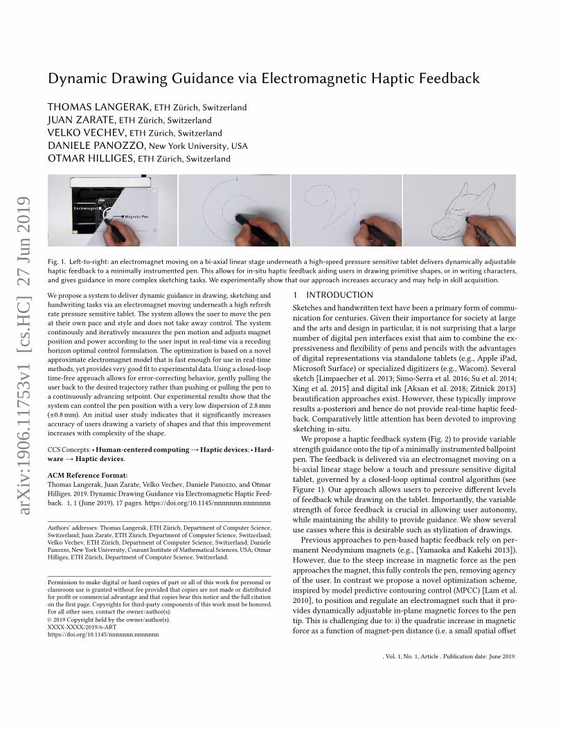
Dynamic Drawing Guidance via Electromagnetic Haptic Feedback

THOMAS LANGERAK, ETH Zürich, SwitzerlandJUAN ZARATE, ETH Zürich, SwitzerlandVELKO VECHEV, ETH Zürich, SwitzerlandDANIELE PANOZZO, New York University, USAOTMAR HILLIGES, ETH Zürich, Switzerland

Fig. 1. Left-to-right: an electromagnet moving on a bi-axial linear stage underneath a high-speed pressure sensitive tablet delivers dynamically adjustablehaptic feedback to a minimally instrumented pen. This allows for in-situ haptic feedback aiding users in drawing primitive shapes, or in writing characters,and gives guidance in more complex sketching tasks. We experimentally show that our approach increases accuracy and may help in skill acquisition.

We propose a system to deliver dynamic guidance in drawing, sketching andhandwriting tasks via an electromagnet moving underneath a high refreshrate pressure sensitive tablet. The system allows the user to move the penat their own pace and style and does not take away control. The systemcontinously and iteratively measures the pen motion and adjusts magnetposition and power according to the user input in real-time via a recedinghorizon optimal control formulation. The optimization is based on a novelapproximate electromagnet model that is fast enough for use in real-timemethods, yet provides very good fit to experimental data. Using a closed-looptime-free approach allows for error-correcting behavior, gently pulling theuser back to the desired trajectory rather than pushing or pulling the pen toa continuously advancing setpoint. Our experimental results show that thesystem can control the pen position with a very low dispersion of 2.8mm(±0.8mm). An initial user study indicates that it significantly increasesaccuracy of users drawing a variety of shapes and that this improvementincreases with complexity of the shape.

CCSConcepts: •Human-centered computing→Haptic devices; •Hard-ware → Haptic devices.

ACM Reference Format:Thomas Langerak, Juan Zarate, Velko Vechev, Daniele Panozzo, and OtmarHilliges. 2019. Dynamic Drawing Guidance via Electromagnetic Haptic Feed-back. 1, 1 (June 2019), 17 pages. https://doi.org/10.1145/nnnnnnn.nnnnnnn

Authors’ addresses: Thomas Langerak, ETH Zürich, Department of Computer Science,Switzerland; Juan Zarate, ETH Zürich, Department of Computer Science, Switzerland;Velko Vechev, ETH Zürich, Department of Computer Science, Switzerland; DanielePanozzo, New York University, Courant Institute of Mathematical Sciences, USA; OtmarHilliges, ETH Zürich, Department of Computer Science, Switzerland.

Permission to make digital or hard copies of part or all of this work for personal orclassroom use is granted without fee provided that copies are not made or distributedfor profit or commercial advantage and that copies bear this notice and the full citationon the first page. Copyrights for third-party components of this work must be honored.For all other uses, contact the owner/author(s).© 2019 Copyright held by the owner/author(s).XXXX-XXXX/2019/6-ARThttps://doi.org/10.1145/nnnnnnn.nnnnnnn

1 INTRODUCTIONSketches and handwritten text have been a primary form of commu-nication for centuries. Given their importance for society at largeand the arts and design in particular, it is not surprising that a largenumber of digital pen interfaces exist that aim to combine the ex-pressiveness and flexibility of pens and pencils with the advantagesof digital representations via standalone tablets (e.g., Apple iPad,Microsoft Surface) or specialized digitizers (e.g., Wacom). Severalsketch [Limpaecher et al. 2013; Simo-Serra et al. 2016; Su et al. 2014;Xing et al. 2015] and digital ink [Aksan et al. 2018; Zitnick 2013]beautification approaches exist. However, these typically improveresults a-posteriori and hence do not provide real-time haptic feed-back. Comparatively little attention has been devoted to improvingsketching in-situ.

We propose a haptic feedback system (Fig. 2) to provide variablestrength guidance onto the tip of a minimally instrumented ballpointpen. The feedback is delivered via an electromagnet moving on abi-axial linear stage below a touch and pressure sensitive digitaltablet, governed by a closed-loop optimal control algorithm (seeFigure 1). Our approach allows users to perceive different levelsof feedback while drawing on the tablet. Importantly, the variablestrength of force feedback is crucial in allowing user autonomy,while maintaining the ability to provide guidance. We show severaluse casses where this is desirable such as stylization of drawings.Previous approaches to pen-based haptic feedback rely on per-

manent Neodymium magnets (e.g., [Yamaoka and Kakehi 2013]).However, due to the steep increase in magnetic force as the penapproaches the magnet, this fully controls the pen, removing agencyof the user. In contrast we propose a novel optimization scheme,inspired by model predictive contouring control (MPCC) [Lam et al.2010], to position and regulate an electromagnet such that it pro-vides dynamically adjustable in-plane magnetic forces to the pentip. This is challenging due to: i) the quadratic increase in magneticforce as a function of magnet-pen distance (i.e. a small spatial offset

, Vol. 1, No. 1, Article . Publication date: June 2019.

arX

iv:1

906.

1175

3v1

[cs

.HC

] 2

7 Ju

n 20

19

https://doi.org/10.1145/nnnnnnn.nnnnnnn

https://doi.org/10.1145/nnnnnnn.nnnnnnn

2 • T. Langerak et al.

Fig. 2. Hardware overview.

can significantly increase the perceived force), ii) the fast pen mo-tion compared to the speed of the linear stage, and iii) the hard topredict behavior of the user. These challenges enforce a very tightcomputational budget from pen motion to magnet actuation, thatis, we need an efficient numerical solution to design a system witha low overall latency.To this end we propose an approximate, yet accurate, model of

the electromagnetic force field that can be evaluated analyticallyand is hence suitable for online control. This model is combinedwith an MPCC-like optimization scheme that iteratively predicts thepen motion and adjusts magnet position and power accordingly. Incontrast to simpler control schemes such as MPC [Faulwasser et al.2009] or PID [Åström and Hägglund 1995] control, our approachdoes not require a timed reference and hence allows users to drawat their desired speed. Furthermore, the optimization scheme allowsfor error-correcting force feedback, gently pulling the user back tothe desired trajectory rather than pushing or pulling the pen to acontinuously advancing setpoint on the trajectory.To assess the proposed feedback mechanism and control algo-

rithm, we performed an user-study with 12 participants. In ourexperiment we focus on drawing primitives such as circles, spirals,and more complex curves. Our results indicate that the haptic feed-back increases both accuracy and precision quantitatively, reducesdrift (i.e., error over time), and that users qualitatively appreciate thesystem. We furthermore, illustrate a number of potential use-casesfor the proposed method such as a support tool for hand drawnsketching and writing, or as in-situ feedback tool for inking, under-and overpainting.

To foster adoption of our technique, and to encourage industrialminiaturization of our device, we will release our reference softwareimplementation and hardware blueprints.

2 RELATED WORKHaptics in touch and pen-based interaction is widely researched. Weprovide a brief overview of the most closely related work, coveringsketching, pen-based interfaces, and magnetic actuation.

Sketching Guidance and Beautification. A number of systems havebeen proposed to provide varying levels of support during sketching,ranging from basic visual guidance to automatic stroke-refinementand vectorization. ShadowDraw guides users by continually updat-ing a shadow underneath their sketch [Lee et al. 2011]. The shadowis generated by first edge-extracting images from a large database,and then analyzing and combining the closest matches to the cur-rent sketch. Limpaecher et al. [2013] improve sketches by replacingstrokes automatically by strokes extracted from drawings stemmingfrom a large database. The authors report that this reduces undo andother correction operations. When tracing images using a techniquecalled underpainting, Su et al. [2014] leverage the underlying imageto perform stroke-refinement in real-time to better fit the gradientinformation underneath. They perform optimization both locallyon a single stroke, and semi and fully globally by considering theinteraction between multiple strokes when no close matches arefound. Xing et al. [2015] perform global similarity analysis acrossmultiple frames to assist during animation tasks and to suggeststrokes that beautify single frames based on past frames.

Inking refers to the process of simplifying sketches and line draw-ings for improved clarity. Several approaches leverage vectorization[Favreau et al. 2016; Hilaire and Tombre 2006], stroke aggregation[Liu et al. 2018], and more recently, convolutional neural networks[Simo-Serra et al. 2018b, 2016] and generative adversarial networks[Simo-Serra et al. 2018a] for this task. Our system is orthogonaland complementary to these approaches, providing active physicalsupport during sketching. We argue that our system is a prime can-didate to be combined with such existing systems to re-enforce theintended or corrected stroke of the user, so that the user not onlyattains a beautified stroke, but also feels the dynamics of creating it.

Haptic Feedback for Pen-Based Interfaces. Haptic feedback has beenstudied in the domain of stylus and tablet interfaces. Poupyrev et al.[2004] used a display instrumented with piezoelectric actuators toprovide tactile feedback and report that users were significantlymore precise in continuous interaction tasks such as sketching. Leeet al. [2004] propose an active stylus containing embedded actuatorsto provide personalized haptic feedback in collaborative settings.Withana et al. [2010] embed a linear actuator inside the pen to con-vey a sense of depth of the screen. Digital rubbing employs a similarsystem, however, for the purpose of tracing over digital images onreal paper [Kim et al. 2008]. The technique requires a solenoid toactivate when the pen passes over a part of the underlying sketch.Because of the delay between measurement and actuation, a simpledead-reckoning movement predictor was applied resulting in signif-icantly better alignment between digital and analog tracings. Somecombined haptic feedback with visual guidance [Portillo et al. 2005].This also promoted research into evaluating visuohaptic systems[Yang et al. 2008].

Haptic interfaces have also been used to increase the accessibilityof GUIs by providing Braille-like feedback on the side of the penduring interaction tasks [Kyung et al. 2008, 2009]. RealPen [Cho et al.2016] increases the realism of sliding over surfaces by mimickingaudio-tactile properties of materials like paper. Pen based input wasalso combined with a 3-DOF device (Phantom Omni) as a handwrit-ing aid for stroke patients [Mullins et al. 2005]. However, since the


Dynamic Drawing Guidance via Electromagnetic Haptic Feedback • 3

user writes in air, the realism of writing on paper is lost. Similarly,there has been some work on tools [Peng et al. 2015; Zoran andParadiso 2013; Zoran et al. 2014].While the benefits of haptic feedback in tablet and pen-based

interfaces have been demonstrated [Cho et al. 2016; Kyung et al.2009; Poupyrev et al. 2004], we argue that a tight adaptive controlloop is necessary to improve perception, accuracy and utility ofsuch approaches (cf. [Kim et al. 2008]). We therefore propose aMPCC-like optimization approach to provide programmable real-time haptic feedback to the user with the aim of increasing accuracyand aesthetic output, without removing user agency.

Magnetic Actuation. Providing magnetically-driven haptic feedbackon tabletops is desirable as the force can be exerted through thesurface without affecting the display. A common approach is usingarrays of controllable electromagnets, combined with permanentmagnets embedded in objects on the surface [Pangaro et al. 2002;Weiss et al. 2011; Yoshida et al. 2006]. Fingerflux byWeiss et al. [2011]provide near-surface haptic feedback before the finger touches thescreen to guide users to appropriate screen locations. Pangaro et al.[Pangaro et al. 2002] model the force-field of each electromagnetand combine these using standard aliasing techniques, allowingdirected movement of multiple objects on the surface. However,moving objects smoothly across the surface is problematic due tothe low resolution of the grid, and the interaction of forces betweenmultiple electromagnets. Furthermore magnets are modeled using asimplification of the Gilbert model, considering attraction betweensingle point poles. In sketching and writing tasks, accuracy is ofthe utmost importance, and thus, we employ a printer-like setup,allowing for smooth movement across a 2D plane and contribute amore accurate EM model based on oriented dipoles.dePENd by Yamaoka and Kakehi [2013] is perhaps the closest

prior research to our system. They move a permanent Neodymiummagnet on a two-axis setup to control the pen of a user. They makeuse of the ferromagnetic feature of the metal tip of regular ballpointpens to attract it. Ourwork differs significantly in the type ofmagnet,its mathematical model and the control strategy, resulting in adifferent user experience and system capabilities. The neodymiummagnet in their work “forces”, rather than guides, the user to followa predefined path. In Yamaoka and Kakehi [2013] the pen is nottracked which results necessitates an open-loop control strategyand little to no user autonomy. The user is allowed to deviate fromthe stroke only slightly by lifting or moving the pen. However, thisinput does not alter the behavior of the magnet. In comparison, oursystem allows the user to move at their own pace through a drawing,and reacts in real-time to user input by altering the position andstrength of the magnet to compensate for user input, thus providingan haptic guidance of the location of the reference path, withoutprescribing a set velocity along the guidance path and not entirelycontrolling the user motion.

Online Path Following. Optimal reference following given real worldinfluences is studied in depth in the control theory literature. Meth-ods like MPC [Faulwasser et al. 2009] optimize the reference pathand the actuator inputs simultaneously based on the system state.MPC is wildly applied to many robotics (e.g., [Mueller and D’Andrea2013]) and graphics applications [Da Silva et al. 2008]. However,

Algorithm 1: Closed Loop Haptic Feedback Control.Function MPCC(x0,w, pp, parameters)[Cl ,Cc ,Cθ ,C Ûθ ] ←compute lag and contour error ▷ Sec 5.2[Cf ,Cd ,Cα ] ←compute force error ▷ Sec 4 & Sec 5.3Jk ← sum(Cl ,Cc ,Cθ ,C Ûθ ,Cf ,Cd ,Cα )[x, u] ←minimize(Jk ) ▷ Sec 5.4

return [x, u]

x0, w← initializewhile drawing not finished do

pp ←Measure pen positionpp,k ← KalmanFilter (pp) ▷ Sec 5.1x0 ← update system states, from sensor dataparameters← update MPCC parameters[xt=1..n, ut=1...n] ←MPCC(x0,w, p, params) ▷ Sec 5x0 ← x1apply(u0)

end

[Aguiar et al. 2008] show that the tracking error for following timed-trajectories can be larger than if following a geometric path only.To address this issue Model Predictive Contouring Control (MPCC)[Lam et al. 2013] has been proposed to follow a time-free reference,optimizing system control inputs for time-optimal progress. MPCCapproaches have been successfully applied in industrial contouring[Lam et al. 2013] and RC racing [Liniger et al. 2014] and in dronecinematography [Nägeli et al. 2017]. We also pose our optimiza-tion problem in the MPCC framework. However, to the best of ourknowledge we are the first to do so in the context of haptic feedbacksystems where one has to consider both a controllable (i.e., the linearstage) and non-controllable (i.e., the user) system. Furthermore, wecontribute a fast approximate electromagnet (EM) model, that givesgood experimental fit, for use in iterative optimization schemes.

3 OVERVIEWThe goal of our work is to provide an integrated software-hardwaresolution that can provide dynamically adjustable force feedback toa regular ballpoint or digital pen. Importantly, we argue that useragency is crucial. This is defined as the user staying in control oftheir actions and the system playing only a supportive role. Hencethe system should never control the user’s motion but only providefeedback. In particular, the user may maintain personal speed andstyle of drawing.

We propose the MagPen system, shown in Figure 2. MagPen con-sists of a high speed pressure sensitive tablet under which an elec-tromagnet is moved on a bi-axial linear stage. The electromagnetdelivers adjustable force feedback to a mostly unmodified pen – weonly attach a small permanent magnet to an otherwise passive ball-point pen. Our proposed optimization scheme (summarized in Alg.1) allows us to adjust the magnet position and strength such thatit gently pulls the pen tip towards a desired stroke, while allowingusers to draw at their desired speed and without fully taking overcontrol. Here we assume that the user traces a known trajectory.



This already enables a number of applications such as practice sup-port in writing of characters or sketching, or as active support ininking or underpainting. We leave integration with a full predictivemodel (e.g., [Aksan et al. 2018]) for future work.

At each time step, we minimize a cost functional over a recedingtime horizon in order to find optimized values for system states xand inputs u. The cost function, here given as high-level abstraction,

minimizex,u

∑Cpath(x, u)︸︷︷︸Eq. 18 & 19

+Cprogress(x, u)︸︷︷︸Eq. 20 & 21

+ Cforce(x, u)︸︷︷︸Eq. 23, 24 & 25

, (1)

serves three main purposes: 1) ensuring that the user stays close tothe desired path, 2) makes progress along it and 3) the user perceiveshaptic feedback of dynamically adjustable force.We first introduce the hardware platform in Sec. 4, including a

novel approximate model of the electromagnet that can be evaluatedin closed form and hence is usable within an iterative optimizationmethod. We then introduce our closed-loop control formulation inSec. 5 that leverages the force behavior model to compute controlinputs for the bi-axial linear stage and for the electromagnet.

4 HARDWAREIn designing the MagPen hardware (Figure 2) we balanced severalimportant aspects. First, the magnetic force must be controlled in afine-grained manner to allow for user agency, essentially ruling outthe use of permanent Neodynium magnets. Second, very small pendisplacement can lead to undesired snapping of the pen tip unless themagnet is adjusted almost instantaneously, due to the quadratic risein magnet attraction as a function of the pen magnet distance (seeaccompanying video for an illustration). This requires low-latencysensing hardware and control software. We chose a display-lesspressure-sensitive tablet since it provides a high framerate. Finally,modeling electromagnetic fields is highly involved and typicallyrequires FEM simulation which would not lend itself for use initerative optimization schemes. This problem is intensified if EMfields overlap and interact, such as in a grid of electromagnets (cf.[Pangaro et al. 2002]). Therefore we move a single electromagneton a bi-axial linear stage and contribute an approximate model ofthe EM field. We leave miniaturization into a tablet form-factor forfuture work but argue that the current form-factor already is aninteresting solution for tracing tables or digital whiteboards.

4.1 Sensing and ActuationOne of our design goals is to provide users with an as unencumberedas possible experience, staying close to the experience of sketchingon pen and paper but allowing for in-situ haptic force feedback.

InMagPen users draw on normal paper with a minimally modifiedballpoint pen. The strokes are recorded by a Sensel Morph (https://sensel.com/) pressure sensitive touch pad. We chose the Senselboard for it’s high spatial resolution (6502DPI), high speed (500Hz)and low latency (2ms). Since the board is designed to be used incombination with different overlays, the sketching surface does notinterfere with the input recognition. Users draw with a 3D printedballpoint pen with a permanent ring magnet mounted in the shaft(see Figure 5).

To deliver haptic feedback to the pen, we move a programmat-ically controlled electromagnet on a bi-axial linear stage directlyunderneath the input sensor. Our implementation leverages the bi-axial system and motors from a Makerbot Replicator 2X 3D printer.We replaced the printer head with an electromagnet (Intertec ITS-MS-5030-12VDC, diameter = 5 cm, height=3 cm, 12 V 11W)mountedon a heatsink and cooled by a fan. The choice of the electromagnetis non-trivial: we need a strong enough electromagnet, fitting inour hardware setup which limits size and heat dissipation, whilenot being too heavy for the linear stage. We employ FEM analysisto make an informed choice with regard to the electromagneticcharacteristics. Our system allows up to 488mN of lateral force (at11 W), with only 2.8mm of point dispersion (see Sec 6.3)

The stepper motors are controlled via a Sparkfun EasyDrivermotor-shield and an Arduino Uno, allowing for micro stepping (afull step is .2mm, we use quarter stepping) of the motors whichincreases the smoothness and accuracy of the magnet motion. Theelectromagnet is controlled via pulse-width modulation (PWM) andan H-Bridge. While allowing for both repulsive and attractive forces,we only use attraction for simplicity.

4.2 Electromagnetic Force ModelWith the hardware platform in place, we require a mathematicalmodel of the electromagnet to compute the attraction force betweenmagnet and pen as a function of their distance. Here we face asignificant challenge: modeling the full EM field, with the help ofa FEM analysis, is not computational feasible in real-time; yet werequire a physically accurate description of the force behavior atevery iteration of our optimization procedure. One of our maincontributions is an approximate model that is efficient to evaluateand provides a very good fit to empirical data. Herewe briefly discussits derivation and we refer to Appendix B and C for additional detailsand for a full validation of the model.The electromagnet core is made of a non-linear ferromagnetic

material. Thus, calculating the physical correct force behavior wouldinvolve pre-computation of a volumetric map of the EM field Bm viaFEM simulation for all levels of the electrical current. The actuationforce on the pen Fp is then given by integrating over the volume ofthe permanent magnet in the pen:

Fp =∭

∇(Mp · Bm(·)

)dxdydz, (2)

where Mp is the magnetization of pen magnet and Bm(·) is the EMfield evaluated at the pen position. Intuitively this can be read asthe force response corresponding to the gradient of the EM fieldevaluated within the volume of the pen magnet. Since this is toocostly to evaluate in real-time, we propose an approximate modelthat is consistent with the underlying physical phenomena.

We make the following two assumptions in our derivations: 1) theelectromagnet and the permanent magnet can be approximated asdipoles (i.e., oriented point magnets), and 2) for the smaller dipole(the permanent magnet in the pen) the out-of-plane vector compo-nent is much larger than the in-plane counterpart. This allows us touse only the vertical component in the calculation of the force. Notethat these simplifications lead only to a small approximation error.Compared to an angle dependent formulation (see Appendix C Eq.


https://sensel.com/

https://sensel.com/


Fig. 3. Illustration of the model to compute the force Fp on dipole mp dueto dipolemm (see Eq. 3). In Eq. 10 we describe the actuation force under theupright pen approximation (β = 0), while in Appendix C we report a moregeneral model for small tilt angles (β ≤ 30◦).

55), a tilt of up to β = 30◦ leads to a max error in our model (Eq.10) equivalent to shifting the distance d by ±3 [mm] (see Figure 4).This uncertainty in d is comparable with the in-plane positioningerror of our overall system (Sec. 6.3). Furthermore, we found thatusers can not perceive a difference in strength when tilting the penin-place.The first approximation allows us to follow the formulation in

[Yung et al. 1998] and to model the force Fp exerted by the electro-magnet dipole mm onto the pen dipole mp (see Figure 3) as:

Fp =3µ0

4πr5mp

[ (⟨mp, rmp⟩

)mm +

(⟨mm, rmp⟩

)mp +

(⟨mp,mm⟩

)rmp −

5(⟨mp, rmp⟩

) (⟨mm, rmp⟩

)r2mp

rmp

], (3)

where µ0 is a constant (see Table 1) and rmp is the 3D vector betweenthe centers of the electromagnet and pen dipoles. The electromagnetcan be seen as magnetic dipole with variable strength, controlledby the dimensionless scalar α ∈ [0, 1].The three vectors needed to compute Eq. 3 can be expressed in

the coordinate system of Figure 3 as

mm = α mm ez, (4)mp = −(mp sin β cosγ ) ed

+(mp sin β sinγ ) et+(mp cos β) ez, (5)

rmp = −(d + hp sin β cosγ ) ed+(hp sin β sinγ ) et+(h − (1 − cos β)hp ) ez. (6)

While providing us with an analytic and differentiable expression,this leads to an equation for the actuation force Fp that depends onthe tilt of the pen through the angles β and γ . With our hardwarethese data are non-trivial to attain. We now leverage our secondassumption by rewriting Eq. 3 with an equivalent pen dipole m̃p,obtained by applying the small tilting angle approximation (cos β ≃

−2 −1.5 −1 −0.5 0 0.5 1 1.5 2

−1

−0.75

−0.5

−0.25

0

0.25

0.5

0.75

1

Fig. 4. In-plane magnetic force as function of position. The horizontal dis-placement between curves (each denoting a different pen-tilt) is the ap-proximation error induced by the upright pen (purple) assumption (anglesdefined in Figure 3).

1 and sin β ≃ 0) to Eq. 5,

m̃p =mp ez , (7)

where the scalar magnetization is given by mp = BrV /µ0. Br isthe residual magnetization of the permanent magnet and V its vol-ume and ez is the z-unit vector. This approximation removes therequirement for tracking the pen tilt. More importantly it drasticallysimplifies the force equation since both dipoles now only have a zcomponent and thus the actuation only depends on the distance dbetween pen and magnet (not on β nor γ ). This provides a simplifiedversion of the 3D distance vector,

r̃mp = −d ed + h ez, (8)

where the vertical distance, h = hm + hp , is constant. Note that thein-plane distance d = ∥pp − pm∥ is one of the variables we seekto control, given the projections of the pen position (pm) and theelectromagnet position (pp) onto the paper plane.

The electromagnet dipole (mm) is mounted in a fixed upright po-sition. Therefore it can be expressed via Eq. 4, without incurring anyapproximation error. The magnetization value of the full-strengthdipolemm , which approximates the electromagnet, can be derivedexperimentally. For this purpose we scan the magnetic field gen-erated by the electromagnet, setting α = 1 and using a hall sensorand adjust the parameters of EM field equation to give a good fit.The full procedure and derivations can be found in Appendix B.Table 1 reports the values ofmm ,mp and h that were used in ourexperiments.

The total force acting on the pen (Eq. 3) can now be decomposedinto the in-plane and vertical force components:

Fp = Fa ed + Fz ez . (9)

Here Fa = Fa ed represents the quantity we seek to control. Bysubstituting the results form Eq. 4, 7 and 8 into Eq. 3 and main-taining only the in-plane contributions (ed direction), we obtainthe expression for the actuation force as function of pen-magnet



Table 1. List of electromagnet model and hardware parameters

Name Value Description

µ0 4π 10−7 [H/m] Vacuum permeabilityBr 1.3 [T] Pen magnet type (NIB N42)V 0.66 [cm3] Pen magnet volumemp 0.683 [A m2] pen dipole (= BrV /µ0)mm 1.286 [A m2] electromagnet dipole (see App. B)h 2.71 [cm] z-distance mm to mp (see App. B)hp 1.40 [cm] height pen-tip to magnet (see Fig. 3)F0 0.488 [N] force factor in Eq. 10), F0 =

3µ0mpmm

4πh4

Fig. 5. Illustration of actuation force Fa, desired force Fθ , and the forcecost-term Cf associate with the difference between those two forces.

separation:

Fa = α F0

©«d

(4 − d2

h2

)h

(1 + d2

h2

) 72

ª®®®¬ ed, (10)

where F0 is a constant force parameter given by the expression,

F0 =3 µ0 mp mm

4 π h4. (11)

Fig. 4 illustrates how the dimensionless ratio within parenthesesin Eq. 10 governs the force strength as function of distance d = ∥rd∥.The actuation force Fa is zero if the two magnets are aligned withone another (d = 0), it has a maximum Fmax

a = 0.9F0 at d = 0.39h,and we can assume there is no more attraction for distances d > 2h.In Table 1 we report the value of F0 we obtained for our setup.We note that the vertical force component Fz from Eq. 9 pulls

the pen downwards. However, during our experiments there wasno significant change in ink thickness or perceived friction whencomparing the drawings with and without electromagnet (i.e., withor without Fz ). For this reason we do not actively optimize forFz in our optimization. Finally, we provide an angle dependentformulation of our model in Appendix C for future use in caseswhere the pen angle is tracked.

5 CLOSED-LOOP CONTROLWith the force behavior model from Eq. 10 we can now deriveour control strategy, such that a force Fa of desired strength is

t=1

t=2

t=3

t=1

t=2

t=3

t=1...n

Set Point

Open-Loop

PenElectromagnet Shortest Distance to Set Point

Time-Dependant Closed-Loop

Time-Independant Closed-Loop

Fig. 6. Overview of different control strategies and their theoretical behav-ior. For sake of simplicity the user is kept at a constant position for alltime-steps. In the case of Open-Loop, the position of the electromagnet isidentical to the setpoint. The setpoint is defined per timestep. For MPC thesetpoint is still defined per timestep, however the EM is at an optimizedposition between the setpoint and the pen. MPCC, on the other hand, alsooptimizes the setpoint based on the pen position (hence, in this station-ary case, the setpoint is also stationary). In a time-dependent setting theelectromagnet might not be close to the pen (open-loop) or in the wrongdirection (time-dependant closed loop). These problems are not present in atime-independent closed loop approach.

exerted onto the pen, in order to keep the user close to the desiredpath. The known path s is parametrized by θ ∈ [0,L], where Lis the length of the path. Note that we do not want to prescribehow fast the user draws the shape and hence for each given penposition pp we first need to establish the closest position on the pathparametrized by s(θ ). Furthermore, we seek to find optimized valuesfor the electromagnet intensity α and the in-plane electromagnetposition pm . We phrase this problem in the MPCC framework [Lamet al. 2013]. Solving the error functional given in Eq. (26) at eachtimestep, yields optimized values for system states x and inputs u.

From a high level perspective, Model Predictive Contour Controlis a closed-loop time-independent control strategy that minimizes acost-function over a fixed receding horizon. As is commonly done inMPC(C), the system is initialized from measurements at t = 0. Thesystem state is then propagated over the horizon with the help of thesystem dynamics (Eq 12). The state vector x contains only variablesthat are controlled by the algorithm (cf. Eq. 13). Only the first ofthe optimized inputs (u0) is then applied to the physical system,transitioning the system state to x1, before iteratively repeating theprocess. This allows for iterative correction of noisy predictions dueto modelling errors.

There are several advantages in using a time-independent closed-loop controls strategy, such as MPCC, over open-loop or time-dependent strategies. First, closed-loop control allows the systemto react to user-input, whereas open-loop control removes all useragency. Both MPC andMPCC are closed-loop control strategies. Themain difference is that MPC tracks a timed reference, prescribing afixed velocity, whereas MPCC follows a time-free trajectory, whichallows the user to progress at the desired speed. Figure 6 illustratesthe expected behavior for a closed-loop versus a timed and time-freestrategy respectively, given that the user decides to slow down orstop moving the pen.



5.1 Dynamics ModelTo control linear stage and electromagnet we require a model f (x, u)describing the system dynamics given its states x and inputs u.

Ûx = f (x, u). (12)

We model the electromagnet with its position pm and magnetintensity α and include a path progress θ .

x = [pm , Ûpm ,α ,θ ] ∈ R6. (13)

The inputs to the system consist of the in-plane electromagnetaccelerations Üpm , and velocities Ûα and Ûθ for magnet intensity andthe spline progress respectively:

u = [Üpm , Ûα , Ûθ ] ∈ R4. (14)

Note that we empirically found that magnet accelerations yieldsmoother motion than using velocities. The state and inputs in themodel are in SI-units. However, the acceleration is converted tostepper motor increments before they are send to the EM controller.

The system model is given by the non-linear ordinary differentialequations using first and second derivatives as inputs:

Üpm = vm , Ûα = vα and Ûθ = vθ , (15)

where v(·) are the external inputs. The continuous dynamics modelÛx = f (x, u) is discretized using a standard forward Euler approach:xt+1 = f (xt , ut ) [Gibbs 2011].

We derive the sets of admissible states χ and inputs ζ empiricallyto conform to the physical hardware constraints of the linear stageand EM specifications (e.g. max voltage). These will be used in thecontrained optimization problem solved in Eq. 27.

The pen position is propagated via a standard linear Kalman filter[Gibbs 2011]. While not an accurate user model, it works well inpractice since the states are recalculated at every timestep.

5.2 Path FollowingWe continuously optimize the EM parameters with the goal of keep-ing the distance between the desired path and the pen minimal.However, we cannot rely on a timed trajectory as is commonly donefor example in MPC formulations (e.g., [Faulwasser et al. 2009]),since we want to give the user freedom in deciding their drawingspeed. To achieve this trade-off, we first need to find the referencepoint s(θ ) itself. Finding the closest point on the path is an op-timization problem itself and hence can not be used within ouroptimization. Similar to recent work in MAV trajectory generation[Gebhardt et al. 2018; Nägeli et al. 2017] we decompose the distanceto the closest point into a contouring and lag error.

We define rθ as the distance between the pen pp and a point s(θ )on the spline, and n as the normalized tangent vector to the splineat that point:

rθ = s(θ ) − pp , (16)

n =s′

∥s′∥ , (17)

with s′ = ∂s(θ )∂θ . The vector rθ can now be decomposed into a

lag error and a contour error (see Figure 7). The lag-error Cl is

Fig. 7. Illustration of lag- and contouring error decomposition.

computed as the projection of rθ on the tangent of s(θ ), while thecontour-error Cc is the component of rθ orthogonal to the normal:

Cl (pp,θ ) = ∥⟨rθ ,n⟩∥2, (18)

Cc (pp,θ ) = ∥rθ − (⟨rθ ,n⟩)n∥2. (19)

Separating lag from contouring error allows us, for example, todifferentiate howwe penalize a deviation outside the path (Cc ), fromencouraging the user to progress forward (Cl ). We furthermoreinclude cost terms to ensure the magnet stays ahead of the pen(Cθ (θ )) and to encourage smooth progress (C Ûθ ( Ûθ )):

Cθ (θ ) = −θ , (20)

C Ûθ ( Ûθ ) = ( Ûθt − Ûθt−1)2. (21)

Finally, we optimize the progress variable θ so that s(θ ) is a com-bination between the closest point and ensuring that the magneteventually does progress to indicate to the user in which directionto continue.

5.3 EM Force ControlLeveraging our physical model for the electromagnetic force Fa (Eq.10), we propose a residual for the desired force Fθ (see Figure 5).The desired force, Fθ pulls the pen towards the target point s(θ ).The cost is modeled with a spring-like behaviour, so that it linearlyincreases with the distance rθ :

Fθ (rθ ) = c F0rθh

erθ , (22)

where c is a scalar that regulates the stiffness of the spring, F0 ascaling of the EM force and h the distance between dipoles in z(set manually). Although simple, this formulation ensures that thehaptic guidance is strong under large deviation from the path whilevanishing as the user approaches the target path (rθ → 0). Notethat the EM force saturates at Fmax

a . Using the expressions for theactuation force Fa (Eq. 10) and desired force (Eq 22) we formulate aquadratic cost term to penalize the difference:

Cf (pm, pp,α) = ∥ Fθ (rθ ) − Fa(d) ∥2. (23)

Since the actuation force Fa declines rapidly with distance, thegradient of Cf goes to 0 for large values ofd causing the optimization



0 50 100 150 2000

20

40

60

80

100

120

PenElectromagnet Reference

x (mm)

y (m

m)

(a) On-path behavior.

0 50 100 150 2000

20

40

60

80

100

120

x (mm)y

(mm

)

(b) Sudden jump in pen position.

0 50 100 150 2000

20

40

60

80

100

120

x (mm)

y (m

m)

(c) Smooth correction.

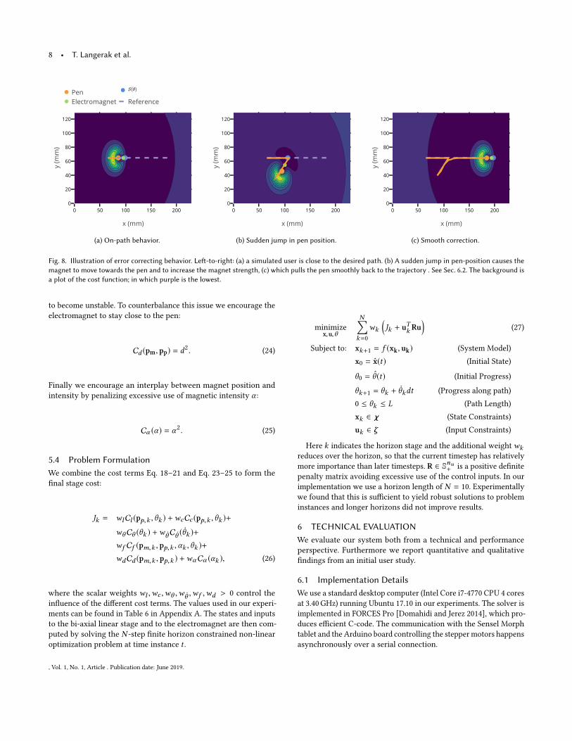
Fig. 8. Illustration of error correcting behavior. Left-to-right: (a) a simulated user is close to the desired path. (b) A sudden jump in pen-position causes themagnet to move towards the pen and to increase the magnet strength, (c) which pulls the pen smoothly back to the trajectory . See Sec. 6.2. The background isa plot of the cost function; in which purple is the lowest.

to become unstable. To counterbalance this issue we encourage theelectromagnet to stay close to the pen:

Cd (pm, pp) = d2. (24)

Finally we encourage an interplay between magnet position andintensity by penalizing excessive use of magnetic intensity α :

Cα (α) = α2. (25)

5.4 Problem FormulationWe combine the cost terms Eq. 18–21 and Eq. 23–25 to form thefinal stage cost:

Jk = wlCl (pp,k ,θk ) +wcCc (pp,k ,θk )+wθCθ (θk ) +w ÛθC Ûθ ( Ûθk )+wf Cf (pm,k , pp,k ,αk ,θk )+wdCd (pm,k , pp,k ) +wαCα (αk ), (26)

where the scalar weights wl ,wc ,wθ ,w Ûθ ,wf ,wd > 0 control theinfluence of the different cost terms. The values used in our experi-ments can be found in Table 6 in Appendix A. The states and inputsto the bi-axial linear stage and to the electromagnet are then com-puted by solving the N -step finite horizon constrained non-linearoptimization problem at time instance t .

minimizex,u,θ

N∑k=0

wk

(Jk + u

Tk Ru

)(27)

Subject to: xk+1 = f (xk, uk) (System Model)x0 = x̂(t) (Initial State)

θ0 = θ̂ (t) (Initial Progress)

θk+1 = θk + Ûθkdt (Progress along path)0 ≤ θk ≤ L (Path Length)xk ∈ χ (State Constraints)uk ∈ ζ (Input Constraints)

Here k indicates the horizon stage and the additional weightwkreduces over the horizon, so that the current timestep has relativelymore importance than later timesteps. R ∈ Snu+ is a positive definitepenalty matrix avoiding excessive use of the control inputs. In ourimplementation we use a horizon length of N = 10. Experimentallywe found that this is sufficient to yield robust solutions to probleminstances and longer horizons did not improve results.

6 TECHNICAL EVALUATIONWe evaluate our system both from a technical and performanceperspective. Furthermore we report quantitative and qualitativefindings from an initial user study.

6.1 Implementation DetailsWe use a standard desktop computer (Intel Core i7-4770 CPU 4 coresat 3.40 GHz) running Ubuntu 17.10 in our experiments. The solver isimplemented in FORCES Pro [Domahidi and Jerez 2014], which pro-duces efficient C-code. The communication with the Sensel Morphtablet and the Arduino board controlling the steppermotors happensasynchronously over a serial connection.



6.2 Error-correcting behaviorAn important design goal is to provide guidance to the user, es-pecially under deviation from the path. Here we analyze how thealgorithm responds to various types of erroneous situations. To thisend we simulate a cooperative user, always following the guidance,but initialize the pen position pp at different off-path positions. Weupdate the pen position via a simple constant velocity model:

pt+1p = ptp +vc

(wv

ptv∥ptv ∥

+wmed

), (28)

where the pen-position pt+1p at timestep t + 1 is updated via theprevious position and a weighted sum of the normalized velocityptv , the exerted force direction ed and a constant velocity factor vc .We analyze a typical but difficult to handle path deviation: a y-

offset in combination with an offset in the direction of negativeθ (backwards). Figure 8 illustrates that our algorithm handles theerror gracefully. In particular the magnet is controlled such that itgently pulls the pen back to the path, rather than pulling directlytowards either the closest point on the path or a steadily advancingsetpoint, as would be the case in traditional control methods.

6.3 Positional dispersionWe now analyze the positional accuracy of the system while iso-lating the user contribution. Note that in the context of drawingthe interesting aspect is not the accuracy of the position of theelectromagnet (stepper motors are discrete and accurate), but theinfluence of the magnet on the pen. To assess this we moved theelectromagnet to random locations and then always back to thecenter of the drawing surface. With a pen being held fully uprightand the magnet at full strength (α = 1) and the user following themagnet passively, this allows us to measure the system’s positionaldispersion. We collected data from 300 repetitions, resulting in amean offset from the target of 2.8mm with a standard deviation(SD) of 0.8mm, indicating that the system can control the pen well.One of the factors that contribute to this dispersion is the vanishingof the actuation force Fa as d → 0. This can lead to the pen motionstopping slightly before it reaches the target.

6.4 LatencyDue to the steepness of the electromagnetic force Fp and the poten-tially fast pen motion, runtime and latency are crucial performancemetrics. The optimization algorithm contributes to both, whereaslatency is dominated by the hardware and I/O. The mean solvetime for a problem instance is 7.4ms (± 3.0ms). Since we do notmanipulate the system state space and pen input is the only mea-surement input this can be expected to be mostly constant. Thehardware and overall system latency adds to the solve time. Weemploy a high-speed camera (1000 fps) to establish the motion (pen)to motion (magnet) latency. This yields an approximate latency of~10ms. Given the combined latency envelope of ~20ms, we did notexperience any abrupt pen snapping in our experiments.

7 USER EVALUATION - CONTROL STRATEGIESWe first conduct a preliminary experiment to validate the choice ofa time-free closed-loop optimization strategy. For this purpose we

PenElectromagnet

Fig. 9. Overview of the different metrics for the preliminary user evaluation.

compare our implementation to a simpler MPC variant and an open-loop strategy (our implementation of dePENd [Yamaoka and Kakehi2013]). The main difference in ours is that s(θ ) is an optimizationvariable itself, whereas MPC used a setpoint that progresses alongthe reference at a predetermined speed.

7.1 ProcedureIn this experiment we asked participantes (N = 12) to draw onecomplex shape (Fig. 11e) in three different conditions: Open-Loop(OL), time-dependent closed loop (MPC), and time-free closed loop(ours). The order of the trials was counterbalanced via a latin-squaredesign.

7.2 MeasuresWe analyze three measures; i) The mean distance from the pen tothe path, ii) the mean distance from the pen position projected ontothe path and s(θ ) along the path and iii) the mean distance fromthe pen to the electromagnet. Taking the mean of the error termsover subjects we ensure equal numbers of datapoints, accountingfor differences in speed. Note that here we assume that the userroughly maintains a constant speed.1 We also gathered qualitativefeedback in the form of a semi-structured interview.A one-way ANOVA with Kruskal-Wallis test was performed for

data analysis.

7.3 ResultsQuantitative. Table 2 summarizes our quantitative findings. Notsurprisingly, the distance from the electromagnet to the pen for (OL)is significant. Since the force exerted on the pen falls off quadraticallywith distance, participants often lost any haptic guidance early on,confirmed via user comments such as “I don’t feel anything” (P3)and “Is the system on?” (P6). Similarly, we see that d(pen, s(θ )) islarger compared to ours by a factor of six.While MPC reduces the distance from the pen to the magnet

(and hence always provides haptic feedback), it does not optimize

1In our full implementation and haptic feedback experiments this assumption is notnecessary. However, the metric used here assumes time-independent datapoints.



0 0.2 0.4 0.6 0.8 1

0

100

200

300

400

500

Open Loop MPC MPCC

Time

Dis

tanc

e(m

m)

(a) Path distance pen-s(θ )

0 0.2 0.4 0.6 0.8 1

2

4

6

8

10

12

Time

Distance(mm)

(b) The euclidean distance from pen-magnet

Fig. 10. Comparison of error over time for a single participant (P1). In 10a there is the inverse u-shape that illustrates that the s(θ ) moves at a different speedthan the user for OL and MPC. Sub-figure 10b show how the EM is relatively close and constant to the pen with MPC and MPCC. With OL the magnet movesaway from the pen. The data is smoothed to increase readability.

Table 2. Mean distance in mm from 1) the pen to the closest point on thepath, 2) distance from pen to s(θ ) along the path, 3) the pen to the electro-magnet and 4) the fraction of the measurements where the electromagnetis more than 15 mm away from the pen (based on Figure 4). All units aregiven in mm.

|pen-path| d(pen, s(θ )) |pen-em|

OL 4.1(±0.7) 38.0(±56.9) 38.2(±25.1)MPC 3.9(±1.3) 45.0(±50.8) 8.6(±1.6)MPCC 2.0(±0.6) 6.2(±0.8) 4.6(±0.9)

for the progress along the path and hence may pull the pen intoundesired directions. For example, MPC produces extreme cornercutting behavior to catch up to the setpoint.Finally, ours has the highest accuracy (H(2)=20.76, p<.001). Fur-

thermore, the setpoint s(θ ) (H(2)=7.362, p <.05) and the electromag-net (H(2)=27.12, p <.001) are closest to the pen. Thus our time-freeformulation overcoms both problems of wrong setpoints (MPC) anda run-away electromagnet, as can happen with strategies proposedin prior-work [Yamaoka and Kakehi 2013].Figure 10 shows that both the distance along the path and the

pen-magnet distance accumulate over time if OL or MPC controlstrategies are employed. Note that this is not the case with ourimplementation (MPCC) and both errors remain low over the entirepath length.

Standard Deviation. Note that for OL and MPC the standard devi-ation is high. This is likely due to the absence of direct couplingbetween user feedback and path progress, which makes it possiblefor the user to lag behind the setpoint significantly (albeit at the costof reduced force feedback). In our implementation the path progressis adjusted to the user’s drawing speed, drastically reducing thestandard deviation and in consequence ensuring delivery of forcefeedback throughout the drawn path.

Qualitative. From our observations we saw that s(θ ) was either infront or behind the user for MPC. This was also confirmed in ourinterview, where people especially commented on the MPC strategy:“The system tries to push me in the wrong direction” (P2) and “It iscounteracting me” (P11). This also resulted in the MPC being theleast preferred option. In contrast with our formulation the magnetremains always slightly ahead of the pen, resulting in users ratingthe MPCC as the most preferred condition. In the words of onesubject this is: “since I still had control” (P9).

Taking both the quantitative and qualitative results into account,we see that our MPCC formulation performs best overall. Open-Loop causes numerous problems, including users not perceiving anyhaptic feedback. This is especially troublesome in settings whereautonomy is desired. In MPC the haptic feedback is perceived, butcan be erroneous. This is especially evident when users do notconform the expected behavior. We therefore only report resultsfrom the MPCC formulation in all further evaluations.

8 USER EVALUATION - HAPTIC FEEDBACKThe impact on task performance and user perception is potentiallythe most important aspect of any haptic feedback system. To assessthese factors we ran an initial controlled user study. In this study,we investigate the overall performance of our MPCC formulationin more detail. To this end we conduct experiments with severaldifferent shapes, and compare to a no-feedback baseline. A firstimpression of the results can be found in Figure 12.

8.1 ProcedureWe invited 12 participants (M=8; F=4, Age=28.2 ± 2.2) into our lab.All subjects were right-handed and did not have any professionaldrawing experience. Before commencing the experiment, users weregiven an introduction to the system functionality and got to experi-ence the system in a self-timed training phase. Only once partici-pants were reasonably confident in the system we continued withthe experiment.



(a) Circle (b) Line (c) Spiral

(d) Sinusoidal (e) Dog (f) Ellipse

Fig. 11. Shapes used in our user tests. Note that the drawing surface onlycontained sparse visual references (shown in blue) and starting positions(orange).

0 50 100 150 2000

20

40

60

80

100

120

x (mm)

y (m

m)

(a) Line

0 50 100 150 2000

20

40

60

80

100

120

x (mm)

y (m

m)

(b) Ellipse

0 50 100 150 2000

20

40

60

80

100

120

x (mm)

y (m

m)

(c) Circle

0 50 100 150 2000

20

40

60

80

100

120

x (mm)

y (m

m)

(d) Spiral

0 50 100 150 2000

20

40

60

80

100

120

x (mm)

y (m

m)

(e) Sinusoidal

0 50 100 150 2000

20

40

60

80

100

120

x (mm)

y (m

m)

(f) Dog

Fig. 12. Selected experimental results. Each shape drawn by different partic-ipants with (orange) and without (blue) guidance, compared to the reference(dotted). Sinusoidal is different from the one in Figure 13a

During the experiment we asked each participant to draw sixbasic shapes, illustrated in Figure 11. Each participant drew eachshape with and without haptic feedback once. The presentationorder of shapes and interface condition was counterbalanced. Thedrawing surface only contained a starting point and, in the caseof more complex shapes, additional visual guidance (shown in redin Figure 11). Furthermore, the participants were shown a scaledversion during task execution (scaled to prevent 1:1 copying).

8.2 Results

Quantitative Results. We first analyze the results quantitatively. Weuse a Hausdorff-like distance [Rockafellar and Wets 2009] as errormetric. To make the metric robust to drawing speed, we re-samplethe drawn path and the reference equidistantly.We then compute thedistance from all re-sampled points to the closest point on the refer-ence. To ensure fairness we also compute the distance from referenceto the drawn path. A Kolmogorov-Smirnov test [Kolmogorov 1933]indicates that both sets are the same and we report uni-directionaldistances.Figure 13a compares the reference (dotted-line) to a sinusoidal

drawn without (blue) and with haptic feedback (orange) by one ofour participants. The path drawn with guidance clearly stays closerto the reference and drifts less. Plotting the error over time confirmsthis observation (Figure 13b), where the error with guidance staysmore or less constant and the guidance-free error continuouslyincreases. Figure 13c, plots the error histogram for both conditionsshowing a longer tail without haptic assistance. This trend holds forall users as can be seen in 14, plotting the pen-reference distancesfor all users.

We conducted a two-way ANOVA on the mean error (computedover all users), as metric for accuracy. Results show a main effect forthe feedback type (F=46.187, p<.001) and for the shapes (F=11.771,p<.001). Post-hoc analysis reveals that the line is statistically sig-nificantly different from all other shapes and we report its resultsseparately. Mean accuracy per shape and significance levels are sum-marized in in Table 3, showing that haptic feedback significantlyimproves accuracy across shapes to 1.871mm (p<.001). While thereis no significant difference for the line, even when including it, weattain a significant accuracy improvement by 1.537mm (p<.001).

Table 3. Mean accuracy in mm. Percentage of error: avg(with)/avg(without)– lower is better. Significance values set to: *p<0.05, **p<0.01, ***p<0.005

With Without

Scenario Mean SD Mean SD Err %

Circle* 2.19 0.90 4.26 2.39 0.51Line 1.18 0.80 1.03 0.84 1.15Spiral*** 2.55 0.75 4.38 1.64 0.58Sinus*** 2.53 0.70 5.08 2.19 0.50Dog*** 2.31 0.54 3.81 1.32 0.60Ellipse*** 2.40 0.56 3.84 1.22 0.62

Qualitative Results. A brief exit interview (see Table 4) shows thatusers subjectively rate the system favourably in terms of accuracy,speed, force and overall performance on a 5-point Likert scale.

Finally, we qualitatively show the effect of using haptic feedbackin Figure 12 using different shapes drawn by different participants.The more complex the shape, the more pronounced the differencebetween the conditions (cf. circle, spiral, dog).

9 ADDITIONAL RESULTSTo further demonstrate the capabilities of our system we illustratepotential use-cases including applications in learning to draw, inoutlining and in inking.



0 50 100 150 2000

20

40

60

80

100

120

x (mm)

y (m

m)

(a) Sinusoidal

0 0.2 0.4 0.6 0.8 1

0

5

10

15

20

Progress along path

Erro

r (m

m)

(b) Error over time

0

0.25

0.5

0.75

1

0 1 2 3 4 5 6 7 8 9 10 11 12 13 14 15 16 17 18 19 20

1

0.75

0.5

0.25

0

Distance (mm)

(c) Pen to reference error histogram.

Fig. 13. Accuracy comparison for a single participant. a reference shape (dotted line) overlaid by path drawn by the same user with (orange) and without(blue) haptic guidance. The absolute error increases over time without error correction b. Error histogram reveals more compact distribution skewed towardslow errors.

Circle Line Spiral Sinusoidal Dog Ellipse

0

2

4

6

8

10

12

With Without

Dis

tanc

e (m

m)

Fig. 14. Distribution of pen to reference distances. All subjects combined.The entries have been trimmed for 10% on both the upper and lower limitin order to increase readability.

Table 4. Survey results. Likert scale: 1=Not Accurate/Slow/Weak/No Im-provement. 5=Very Accurate/Fast/Strong/Much Improvement.

Question Accuracy Speed Force Improvement

Mean 4.33 4.00 3.50 4.50SD 0.62 0.91 0.86 0.90

Calligraphy: Figure 15b and Figure 15d illustrate writing of flour-ished characters, with only minimal visual guidance (single startingpoint). Although an offset from the reference path remains, the linesare smooth and the overall shape is close to the desired characters.

Drawing teaching aid: Connect-the-dots exercises are often used toteach children motor skills as well as stroke ordering. Figure 15fshows results from a similar exercise performed with our system,yet using much fewer dots as visual guidance than a paper version.

Outlining & inking: Figure 17 illustrates the effect of two core capabil-ities of the proposed approach. Here we first outline the proportionsof the dragon head and then use different pens to ink-in the details.

(a)

0 50 100 150 2000

20

40

60

80

100

120

x (mm)

y (m

m)

(b)

(c)

0 50 100 150 2000

20

40

60

80

100

120

x (mm)

y (m

m)

(d)

(e)

0 50 100 150 2000

20

40

60

80

100

120

x (mm)

y (m

m)

(f)

Fig. 15. Overview of use cases: calligraphy (15b and 15d) and drawingexercises (15f). Figures 15a, 15c, 15e show the guidance given during theexperiment.

Note that the system provides haptic guidance but allows the user todraw the shape in different styles and with varying high-frequencydetail, while maintaining similarity to the reference shape. This is adirect consequence of using time-free closed loop control approach,as is alluded to in Sec. 7. In this case, all four variants were drawnwithout changes to the system or desired path.

10 DISCUSSIONFrom a technical perspective we can we can conclude our time-independent closed-loop control formulation, provides qualitativelyand quantitatively better results than simpler approaches. Open-loop control might lead to complete loss of feedback due to differ-ences in speed. This is solved in a closed-loop setting. However,



time-dependent implementations can maintain haptic feedback butthe perceived direction of the feedback maybe wrong. This is solvedby our time-independent implementation, where s(θ ) is part of theoptimization problem.Our haptic feedback experiments indicate that the proposed ap-

proach indeed increases accuracy in drawing tasks and that usersrate the system favorably. We did not find a significant differencefor the straight line. This may be explained by user feedback, thatthe maximum speed of the linear stage is a limiting factor in thecurrent implementation. We leave faster magnet positioning forfuture work.

Two aspects from the exit interviews are noteworthy. First, thereis a high standard deviation in how users rated the perceived force.We hypothesize that this is due to the way users operate the pen,with some leveraging the full arm and others rely more on thewrist. We note that our palm rejection implementation is simple andmay have contributed to this. Furthermore, some users indicatedthat they had the feeling that their drawings without feedback weremore accurate once they experienced the haptic guidance, indicatingthe possibility of short-term muscle memory. Long-term learninghowever is difficult to evaluate experimentally and goes beyond thescope of this paper.Finally, during our experiments we noticed a tendency to cut

corners, well illustrated in the case of the sinusoidal (see Figure 13a,12e). To unpack this issue further, we performed an experiment insimulation, with the user model from Eq. 28, tracing references withincreasingly sharp angles (see Figure 16). The plot clearly showsan increase in error with increase in curvature. It has been shownthat humans trade-off speed and accuracy in tracing tasks and thatthey slow down when tracing high-curvature paths [Accot and Zhai1997]. Currently our implementation does not take curvature of thereference into account but it would be straightforward to penalizethe progress θ along the reference according to its curvature.

11 LIMITATIONS & FUTURE WORKThere are, of course, some limitations to our current approach. First,the maximum speed of the linear stage we used is relatively slow.This causes users to slow down their drawing speed. This could beovercome via a faster bi-axial linear stage, which are commerciallyavailable but expensive. A potentially more interesting and scalabledirection would be to extend the proposed magnet model towards agrid of electromagnets. However, the interaction between severaloverlapping EM fields with a moving permanent magnet are non-trivial to model and would require significant research.Once the hardware-induced speed limitation is overcome, effi-

cient closed-loop control approaches become an interesting direc-tion for future work, since faster pen motion would also tightenthe latency and accuracy budget. In the context of sensing it wouldbe interesting to incorporate a mechanism to reconstruct the tilt ofthe pen. This could be achieved for example via an accelerometerbuilt into the pen or via a grid of hall-sensors underneath the sur-face. Information on the pen tilt could then be combined with theangle dependent formulation of our EM model (see Appendix B).Furthermore, we believe there are many research opportunities incombining our approach with other sketch and ink beautification

−50 0 5050

60

70

80

90

100

110

x (mm)

y (m

m)

(a) 36.9 ◦

−50 0 5050

60

70

80

90

100

110

x (mm)

y (m

m)

(b) 46.1◦

−50 0 5050

60

70

80

90

100

110

x (mm)

y (m

m)

(c) 57.1◦

−50 0 5050

60

70

80

90

100

110

x (mm)

y (m

m)

(d) 73.3◦

−0.4 −0.2 0 0.2 0.4

0

2.5

5

7.5

0.0 6.9 13.9 21.1 28.7 36.9 46.1 57.173.7

Progress along path

Erro

r (m

m)

Fig. 16. Curvature dependent error. Insets a-c show increasingly sharpcornered references (dotted lines) and the resulting pen trajectory (in simu-lation). x-axis is normalized for cord length, so that all angles can be directlycompared. Bottom: error over 9 different levels of curvature (in degrees).

approaches (e.g., [Simo-Serra et al. 2018a, 2016; Xing et al. 2015]).Particularly interesting would be to leverage fully predictive models(e.g., [Aksan et al. 2018]) in order to overcome the need for a knownreference.Another interesting direction of research is connected to the

observation that different users perceive the feedback at differentstrength levels. This could be due to grip strength, or movementfrom the shoulder rather than wrist. A stronger (i.e., bigger) electro-magnet could increase the dynamic range. However, this would haveto be carefully counterbalanced with weight and heat dissipationconcerns as well as with a loss in accuracy towards the center ofthe electromagnet (the force goes to zero as rd → 0).

We believe that it could be an interesting direction for future workto combine our approach with different types of haptic feedback,either environment mounted or body-worn. Moreover, we have sofar focused our attention towards drawing applications. However,electromagnetic feedback in combination with spatial actuationmaybe interesting in other settings. For example, a magnet mountedto a robotic arm could deliver contact-less feedback in VR scenarios.



Fig. 17. Different variants of the same dragon, drawn with identical systemsettings by a novice. Each pair of drawings used with different tools. Firsta pencil for proportions and a fine-liner (top) or pencil (bottom) to ink-in details. Multi-stroke lines are achieved by approaching each seperateinstance as a new figure, the system is trigger by a pen lift.

It would also be interesting to investigate how to best exploit thesystem capabilities in the context of motor memory and learning.

12 CONCLUSIONSWe have proposed MagPen, a system that delivers dynamically ad-justable guidance in drawing and sketching tasks. We have detailedour hardware setup and discussed a novel model of the electro-magnetic interactions in the system. The proposed model can beevaluated analytically and is hence suitable for iterative, real-timeoptimization approaches. We have furthermore demonstrated thatthe assumptions of dipole magnets and an upright pen lead onlyto a small approximation error. However, we have included a an-gle dependent formulation that maybe used in future work, wherepen-tilt information is available.We have also discussed a novel optimization scheme based on

the MPCC framework that leverages the EM model, in order tooptimize the system states and its inputs over a receding horizon viasolving a stochastic optimal control problem at each timestep. Ourformulation has been designed to provide dynamically adjustableforces and automatically adjusts magnet position and strength.

Our experiments have shown that the proposed hardware-softwaresolution is effective in improving accuracy and in guiding users ina variety of drawing tasks, without taking away agency and controlfrom the user. We believe this is an interesting first step towardsmany exciting applications of electromagnetic haptic feedback. In or-der to foster future research we will release all hardware schematicsand software source code to the public.

ACKNOWLEDGMENTSThis work was supported in part the Hasler Foundation (Switzer-land), ERC (OPTINT StG-2016-717054) NSF (IIS-CAREER 1652515

and OAC:1835712), a gift from nTopology, and a gift from AdobeResearch. We thank all participants for taking part in our experi-ments.

REFERENCESJohnny Accot and Shumin Zhai. 1997. Beyond Fitts’ law: models for trajectory-based

HCI tasks. In Proceedings of the ACM SIGCHI Conference on Human factors in com-puting systems. ACM, 295–302.

A. Pedro Aguiar, Joao P. Hespanha, and Petar V. Kokotovic. 2008. Performance limita-tions in reference tracking and path following for nonlinear systems. Automatica44, 3 (2008), 598 – 610. https://doi.org/10.1016/j.automatica.2007.06.030

Emre Aksan, Fabrizio Pece, and Otmar Hilliges. 2018. DeepWriting: Making Digital InkEditable via Deep Generative Modeling. In SIGCHI Conference on Human Factors inComputing Systems (CHI ’18). ACM, New York, NY, USA.

Karl Johan Åström and Tore Hägglund. 1995. PID controllers: theory, design, and tuning.Vol. 2. Instrument society of America Research Triangle Park, NC.

Youngjun Cho, Andrea Bianchi, Nicolai Marquardt, and Nadia Bianchi-Berthouze. 2016.RealPen: Providing Realism in Handwriting Tasks on Touch Surfaces using Auditory-Tactile Feedback. In Proceedings of the 29th Annual Symposium on User InterfaceSoftware and Technology. ACM, 195–205.

M. Da Silva, Y. Abe, and J. PopoviÄĞ. 2008. Simulation of Human MotionData using Short-Horizon Model-Predictive Control. Computer Graphics Fo-rum 27, 2 (2008), 371–380. https://doi.org/10.1111/j.1467-8659.2008.01134.xarXiv:https://onlinelibrary.wiley.com/doi/pdf/10.1111/j.1467-8659.2008.01134.x

Alexander Domahidi and Juan Jerez. 2014. FORCES Professional. embotech GmbH(http://embotech. com/FORCES-Pro).

T. Faulwasser, B. Kern, and R. Findeisen. 2009. Model predictive path-following forconstrained nonlinear systems. In Proceedings of the 48h IEEE Conference on Decisionand Control (CDC). 8642–8647. https://doi.org/10.1109/CDC.2009.5399744

Jean-Dominique Favreau, Florent Lafarge, and Adrien Bousseau. 2016. Fidelity vs.simplicity: a global approach to line drawing vectorization. ACM Transactions onGraphics (TOG) 35, 4 (2016), 120.

Christoph Gebhardt, Stefan Stevsic, and Otmar Hilliges. 2018. Optimizing for Aestheti-cally Pleasing Quadrotor CameraMotion. ACMTransactions on Graphics (Proceedingsof ACM SIGGRAPH) 37, 4, Article 90 (2018), 11 pages.

Bruce P Gibbs. 2011. Advanced Kalman filtering, least-squares and modeling: a practicalhandbook. John Wiley & Sons.

Xavier Hilaire and Karl Tombre. 2006. Robust and accurate vectorization of linedrawings. IEEE Transactions on Pattern Analysis and Machine Intelligence 28, 6 (2006),890–904.

Hyunjung Kim, Seoktae Kim, Boram Lee, Jinhee Pak, Minjung Sohn, Geehyuk Lee,and Woohun Lee. 2008. Digital rubbing: playful and intuitive interaction techniquefor transferring a graphic image onto paper with pen-based computing. In CHI’08Extended Abstracts on Human Factors in Computing Systems. ACM, 2337–2342.

Andrey Kolmogorov. 1933. Sulla determinazione empirica di una lgge di distribuzione.Inst. Ital. Attuari, Giorn. 4 (1933), 83–91.

Ki-Uk Kyung, Jun-Young Lee, and Junseok Park. 2008. Haptic stylus and empiricalstudies on braille, button, and texture display. BioMed Research International 2008(2008).

Ki-Uk Kyung, Jun-Young Lee, and Mandayam A Srinivasan. 2009. Precise manipulationof GUI on a touch screen with haptic cues. In EuroHaptics conference, 2009 andSymposium on Haptic Interfaces for Virtual Environment and Teleoperator Systems.World Haptics 2009. Third Joint. IEEE, 202–207.

Denise Lam, Chris Manzie, and Malcolm Good. 2010. Model predictive contouringcontrol. In Decision and Control (CDC), 2010 49th IEEE Conference on. IEEE, 6137–6142.

Denise Lam, Chris Manzie, and Malcolm C Good. 2013. Model predictive contouringcontrol for biaxial systems. IEEE Transactions on Control Systems Technology 21, 2(2013), 552–559.

Johnny C Lee, Paul H Dietz, Darren Leigh, William S Yerazunis, and Scott E Hudson.2004. Haptic pen: a tactile feedback stylus for touch screens. In Proceedings ofthe 17th annual ACM symposium on User interface software and technology. ACM,291–294.

Yong Jae Lee, C Lawrence Zitnick, and Michael F Cohen. 2011. Shadowdraw: real-timeuser guidance for freehand drawing. In ACM Transactions on Graphics (TOG), Vol. 30.ACM, 27.

Alex Limpaecher, Nicolas Feltman, Adrien Treuille, and Michael Cohen. 2013. Real-timedrawing assistance through crowdsourcing. ACM Transactions on Graphics (TOG)32, 4 (2013), 54.

Alexander Liniger, Alexander Domahidi, and Manfred Morari. 2014. Optimization-based autonomous racing of 1:43 scale RC cars. Optimal Control Applications andMethods (2014). https://doi.org/10.1002/oca.2123

Chenxi Liu, Enrique Rosales, and Alla Sheffer. 2018. StrokeAggregator: consolidatingraw sketches into artist-intended curve drawings. ACM Transactions on Graphics


https://doi.org/10.1016/j.automatica.2007.06.030

https://doi.org/10.1111/j.1467-8659.2008.01134.x

http://arxiv.org/abs/https://onlinelibrary.wiley.com/doi/pdf/10.1111/j.1467-8659.2008.01134.x

https://doi.org/10.1109/CDC.2009.5399744

https://doi.org/10.1002/oca.2123


(TOG) 37, 4 (2018), 97.M.W. Mueller and R. D’Andrea. 2013. A model predictive controller for quadrocopter

state interception. In Proceedings of the European Control Conference (ECC), 2013.1383–1389. http://ieeexplore.ieee.org/xpls/abs_all.jsp?arnumber=6669415

James Mullins, Christopher Mawson, and Saeid Nahavandi. 2005. Haptic handwritingaid for training and rehabilitation. In Systems, Man and Cybernetics, 2005 IEEEInternational Conference on, Vol. 3. IEEE, 2690–2694.

Tobias Nägeli, Lukas Meier, Alexander Domahidi, Javier Alonso-Mora, and OtmarHilliges. 2017. Real-time Planning for Automated Multi-View Drone Cinematogra-phy. ACM Transactions on Graphics (Proceedings of ACM SIGGRAPH).

Gian Pangaro, DanMaynes-Aminzade, and Hiroshi Ishii. 2002. The actuated workbench:computer-controlled actuation in tabletop tangible interfaces. In Proceedings of the15th annual ACM symposium on User interface software and technology. ACM, 181–190.

Huaishu Peng, Amit Zoran, and François V Guimbretière. 2015. D-Coil: A Hands-onApproach to Digital 3D Models Design. In Proceedings of the 33rd Annual ACMConference on Human Factors in Computing Systems. ACM, 1807–1815.

O Portillo, Carlo Alberto Avizzano, Mirko Raspolli, and Massimo Bergamasco. 2005.Haptic desktop for assisted handwriting and drawing. In ROMAN 2005. IEEE In-ternational Workshop on Robot and Human Interactive Communication, 2005. IEEE,512–517.

Ivan Poupyrev, Makoto Okabe, and Shigeaki Maruyama. 2004. Haptic feedback for pencomputing: directions and strategies. In CHI’04 extended abstracts on Human factorsin computing systems. ACM, 1309–1312.

R Tyrrell Rockafellar and Roger J-B Wets. 2009. Variational analysis. Vol. 317. SpringerScience & Business Media.

Edgar Simo-Serra, Satoshi Iizuka, and Hiroshi Ishikawa. 2018a. Mastering sketching:adversarial augmentation for structured prediction. ACM Transactions on Graphics(TOG) 37, 1 (2018), 11.

Edgar Simo-Serra, Satoshi Iizuka, and Hiroshi Ishikawa. 2018b. Real-time data-driveninteractive rough sketch inking. ACM Transactions on Graphics (TOG) 37, 4 (2018),98.

Edgar Simo-Serra, Satoshi Iizuka, Kazuma Sasaki, and Hiroshi Ishikawa. 2016. Learningto simplify: fully convolutional networks for rough sketch cleanup. ACM Transac-tions on Graphics (TOG) 35, 4 (2016), 121.

Qingkun Su, Wing Ho Andy Li, Jue Wang, and Hongbo Fu. 2014. EZ-sketching: three-level optimization for error-tolerant image tracing. ACM Transactions on Graphics33, 4 (2014).

Malte Weiss, Chat Wacharamanotham, Simon Voelker, and Jan Borchers. 2011. Finger-Flux: near-surface haptic feedback on tabletops. In Proceedings of the 24th annualACM symposium on User interface software and technology. ACM, 615–620.

Anusha Withana, Makoto Kondo, Yasutoshi Makino, Gota Kakehi, Maki Sugimoto, andMasahiko Inami. 2010. ImpAct: Immersive haptic stylus to enable direct touch andmanipulation for surface computing. Computers in Entertainment (CIE) 8, 2 (2010),9.

Jun Xing, Li-Yi Wei, Takaaki Shiratori, and Koji Yatani. 2015. Autocomplete hand-drawnanimations. ACM Transactions on Graphics (TOG) 34, 6 (2015), 169.

Junichi Yamaoka and Yasuaki Kakehi. 2013. dePENd: augmented handwriting systemusing ferromagnetism of a ballpoint pen. In Proceedings of the 26th annual ACMsymposium on User interface software and technology. ACM, 203–210.

Xing-Dong Yang, Walter F Bischof, and Pierre Boulanger. 2008. Validating the perfor-mance of haptic motor skill training. In 2008 Symposium on Haptic Interfaces forVirtual Environment and Teleoperator Systems. IEEE, 129–135.

Shunsuke Yoshida, Haruo Noma, and Kenichi Hosaka. 2006. Proactive desk II: Develop-ment of a new multi-object haptic display using a linear induction motor. In VirtualReality Conference, 2006. IEEE, 269–272.

Kar W Yung, Peter B Landecker, and Daniel D Villani. 1998. An analytic solution for theforce between two magnetic dipoles. Physical Separation in Science and Engineering9, 1 (1998), 39–52.

C Lawrence Zitnick. 2013. Handwriting beautification using token means. ACMTransactions on Graphics (TOG) 32, 4 (2013), 53.

Amit Zoran and Joseph A Paradiso. 2013. FreeD: a freehand digital sculpting tool. InProceedings of the SIGCHI Conference on Human Factors in Computing Systems. ACM,2613–2616.

Amit Zoran, Roy Shilkrot, Pragun Goyal, Pattie Maes, and Joseph A Paradiso. 2014.The wise chisel: The rise of the smart handheld tool. IEEE Pervasive Computing 13,3 (2014), 48–57.

A NOTATION AND VARIABLESWe summarize the notations used in this paper in Table 5. Pleaserefer to Table 6 for all weights, constants and parameters used inour implementation.

Table 5. List of notations used on this work.

Symbol Description

xt State of the system at time tut Input to the system at time tC(·) Cost term for optimization problemw(·) Weight for the optimization cost termsJk Cost function (=

∑wiCi ) for the k-time prediction

χ Set of state constraintsζ Set of input constraintsdt Sampling timemm Magnetic dipole of the electromagnetmp Magnetic dipole of the pen magnetm̃p Approx. of mp, with only ez component and cos β ≃ 1rmp 3D Vector distance from mm to mpr̃mp 3D Vector distance from mm to m̃ppp Pen tip positionpm Center of electromagnet, projected into paper planerd in-plane vector rd = pm − pped unity vector that goes from ed = rd/∥rd∥d in-plane separation between pp and pm, i.e d = ∥rd∥h = hm + hp , i.e vertical distance between mp and m̃pα intensity of the electromagnet (PWM input)Fa Actuation force on the pen, from pp to pmθ Control parameter to progress along the desired paths(θ ) Current desired point in the pathrθ in-plane vector rθ = s(θ ) − pmFθ Desired force on the pen, from pp to s(θ )n The normalized tangent at s(θ )

Table 6. List of variables and optimization weights used in this work.

Variable N wl wc wθ w Ûθ wf

Value 10 1.5 1.5 10. 0.1 10.

cont.Variable wd wα c wv wm vC

Value 0.05 7. 5. 1. 1. 0.1

B ELECTROMAGNET DIPOLE EQUIVALENTHere we describe the experimental validation of the dipole modelfor our electromagnet, that allows us to compute the force thatthe electromagnet exerts onto the permanent magnet on the pen.This interaction is minimal at distance h, when the electromagnetand pen are located directly above each other (See Figure 5). Themagnetic field generated by a dipole mm (electromagnet) at theposition of dipole mp (pen) can be written as,

Bm(rmp,mm) =µ04π

(3rmp

(mm · rmp

)r5mp

− mm

r3mp

)(29)

where the vector rmp is the vector that goes from mm to mp (seeFigure 3). The magnetic field Bm is well described in a cylindrical


http://ieeexplore.ieee.org/xpls/abs_all.jsp?arnumber=6669415


0 2 4 6 8 10

0

0.002

0.004

0.006

0.008

0.01

0.012

Data Fit

x (cm)

Bz,

m (

T)

Fig. 18. 3D overview of all data points. The x,y axis are position and thez-axis is B(z)2

system centered on the dipole and with the z-axis aligned on thedirection of mm. Taking only the z component on Eq. 29 and usingthe definitions of rmp (Eq. 8) and mm (Eq. ??) we arrive at,

Bm,z (d) =µ0αmm

4π©« 2h2 − d2(d2 + h2

) 5 2ª®¬ (30)

We measure the z-component of the magnetic field generated bythe electromagnet to compare it with the dipole prediction of Eq.30. We use a hall sensor (Allegro A1324, sensitivity is 5 mV/G)2 tomeasure the z-magnetic flux at a fix height hm , where the magnet ofthe pen would be. Setting the electromagnet to α = 1 and moving itin a grid we attain multiple readings of the hall sensor for differentelectromagnet positions pm. We present the obtained magnetic fieldplotted in Figure 18, top.

Due to symmetry over the z-axis we expect for Bm,z , we re-plot allpoints as a function of distance ds = ∥ps − pm∥, with ps = (0, 0) thein-plane position of the hall sensor. In turn, Eq. 30 can be expressed

2http://www.farnell.com/datasheets/1538021.pdf

in the form,

Bm,z (ds ) = C12C2

2 − d2s(

d2s +C22

)5/2 (31)

where we have defined two parameters used for the fitting,

C1 =µ0αmm

4π(32)

C2 = h (33)

The bottom plot of Figure 18 shows the measured data for mag-netic flux Bm,z (ds ) and the fitting to Eq. 31, from which we obtainedC1 = −1.276 10−07 and C2 = 2.713 10−02. By replacing these valuesin equations 32 and 33, we observe that our system can be describedby the valuesmm = 1.286 [A m2] and h = 2.71 [cm]. We want toemphasize the excellent agreement in Figure 18 between the experi-mental values and the proposed dipole model for the electromagnet.However, we should note that the experimental points show a flat-tening of Bm,z (x) for values of x < 3 [mm], that translates intosmaller values of forces in that region, as Fa ∝ ∇Bm,z . This experi-mental behaviour may explain the position dispersion results wereport in Section 6.3.

C ANGLE AWARE DIPOLE-DIPOLE MODELIn this section we describe the derivation of the dipole-dipole modelfor the in-plane actuation force, in the case of considering a pentilt β of the pen. Please refer to the schematic Figure 3 for vectornotations we use in this section. The coordinate system is given by,

ed =pm − pp| |pm − pp | |

(34)

ez = [0, 0, 1]T (35)et = ed × ez (36)

with ed the in-paper-plane distance from the pen contact point tothe electromagnet center projection, ez the vertical out-of-planedirection and et the orthogonal vector to the former two.The dipole-dipole expression for the force acting on mp due to

mm and separated by rmp is given by Eq. 3), repeated here:

Fp =3µ0

4πr5mp

[ (⟨mp, rmp⟩

)mm +

(⟨mm, rmp⟩

)mp +

(⟨mp,mm⟩

)rmp −

5(⟨mp, rmp⟩

) (⟨mm, rmp⟩

)r2mp

rmp

], (37)

The two dipoles and the vector distance between them can beexpressed in the proposed coordinate system as,

mm = α mm ez (38)mp = −(mp sin β cosγ ) ed

+(mp sin β sinγ ) et+(mp cos β) ez (39)

rmp = −(d + hp sin β cosγ ) ed+(hp sin β sinγ ) et+(h − (1 − cos β)hp ) ez (40)


http://www.farnell.com/datasheets/1538021.pdf


and the three scalar products of equation 37,

⟨mm, rmp⟩ = α mm [h − (1 − cos β)hp ] (41)⟨mp, rmp⟩ = mp [− sin β cosγ (d + hp sin β cosγ )

+ sin β2 sinγ 2hp + cos β(h − hp (1 − cos β))](42)⟨mm,mp⟩ = αmmmp cos β (43)

We continue the deduction of Fp by substituting Eq. 38—43 intothe main expression Eq. 37. However, by following that path wewouldn’t necessarily attain information on how strong the actuationforce depends on the tilting angles β and γ . Here we take a differentpath. Based on the geometry of our system, we consider the caseswhere the pen is tilted by only a small angle (β < 30o ). We introducethis small-angle approximation by keeping only the first order termsin β ,

sin β ≈ β (with β in radians) (44)cos β ≈ 1 (45)

As an indication of what this approximation means, for an angleβ = 30◦, the difference between using sin β or cos β or their approx-imations forms (Eq. 44 and 45) is 5% and 15 %, respectively. Underthe small-β approximation, the dipoles’ vectors are,

mm = α mm ez (46)mp ≃ −mpβ cosγed +mpβ sinγet +mp ez (47)

and the distance between dipoles,

rmp ≃ −(d + hpβ cosγ ) ed + hpβ sinγ et + h ez (48)

with the length of that distance, at first order on β ,

rmp ≃ d2 + h2 + 2dhpβ cosγ (49)

In turn, the scalar products (Eq. 41—43) can be written as,

⟨mm, rmp⟩ ≃ α mmh (50)⟨mp, rmp⟩ ≃ mp [−β cosγd + h] (51)⟨mm,mp⟩ ≃ α mmmp (52)

We can now substitute these expressions into the main forceequation 37. As we do in Section 4.2, we consider only the termsthat contribute to the component ed of the force. Keeping only theseterms that contain β up to the first order,

F(d)p =3µ0αmmmp

4πr5mp

[−d + 5dh2

r2mp− hβ cosγ − hpβ cosγ+

+5h2hpβ cosγ

r2mp− 5hd2β cosγ

r2mp

]ed (53)

=3µ0αmmmp

4π (h2 + d2)5/2

[−d(d2 + h2) + 5dh2

(h2 + d2)+

β cosγ

(−h − hp +

5(h2hp − hd2)(h2 + d2)

−5d2h2hp(h2 + d2)2

)]ed

(54)

F(d)p = α F0 [ f0(d) + β cosγ f1(d) ] ed (55)

where we define,

F0 =3 µ0 mp mem

4 π h4. (56)

f0(d) =d

(4 − d2

h2

)h

(1 + d2

h2

) 72

(57)

f1(d) =1 + hp

h(1 + d2

h2

) 52+5(hph +

d2

h2

)(1 + d2

h2

) 72−5(hph

) (d2

h2

)(1 + d2

h2

) 92

(58)

Note that by considering the case β = 0 in Eq. 55, we recoverwhat we obtain in the Sec. 4.2 for Fa. That means that the equationfor F(d)p we obtained in this Appendix subsumes the cases of thepen being tilted by a small angles, and it can be used in future EMactuated systems which may be able to track β and γ .


Dynamic Drawing Guidance via Electromagnetic Haptic ...

Documents

Transcript of Dynamic Drawing Guidance via Electromagnetic Haptic ...