Algorithms: Matrix-Matrix Multiplication - University of Illinois

Riemann–Hilbert Problems, Matrix OrthogonalPolynomials and Discrete Matrix Equations with
Singularity Confinement
By G.A. Cassatella-Contra and M. Manas∗
In this paper, matrix orthogonal polynomials in the real line are described interms of a Riemann–Hilbert problem. This approach provides an easy derivationof discrete equations for the corresponding matrix recursion coefficients. Thediscrete equation is explicitly derived in the matrix Freud case, associatedwith matrix quartic potentials. It is shown that, when the initial condition andthe measure are simultaneously triangularizable, this matrix discrete equationpossesses the singularity confinement property, independently if the solutionunder consideration is given by the recursion coefficients to quartic Freudmatrix orthogonal polynomials or not.
1. Introduction
The study of singularities of the solutions of nonlinear ordinary differentialequations and, in particular, the quest of equations whose solutions are freeof movable critical points, the so called Painleve property, lead, more than100 years ago, to the Painleve transcendents, see [1] (and [2] for a recentaccount of the state of the art in this subject). The Painleve equations arerelevant in a diversity of fields, not only in Mathematics but also, for example,in Theoretical Physics and in particular in 2D Quantum Gravity and TopologicalField Theory, see for example, [2].
∗Address for correspondence: M. Manas, Departamento de Fısica Teorica II, Universidad Compltense,28040-Madrid, Spain; e-mail: [email protected]
DOI: 10.1111/j.1467-9590.2011.00541.x 252STUDIES IN APPLIED MATHEMATICS 128:252–274C© 2011 by the Massachusetts Institute of Technology

Riemann–Hilbert Problems and Singularity Confinement 253
A discrete version of the Painleve property, the singularity confinementproperty, was introduced for the first time by Grammaticos et al. in 1991 [3],when they studied some discrete equations, including the dPI equation (discreteversion of the first Painleve equation), see also the contribution of theseauthors to [2]. For this equation they realized that if eventually a singularitycould appear at some specific value of the discrete independent variable itwould disappear after performing few steps or iterations in the equation.This property, as mentioned previously, is considered by these authors as theequivalent of the Painleve property [1] for discrete equations. Ramani et al.also derived some discrete versions of the other five Painleve equations [4, 5].See also the interesting papers [6] and [7].
Freud orthogonal polynomials in the real line [8] are associated to the weight
wρ(x) = |x |ρe−|x |m , ρ > −1, m > 0.
Interestingly, for m = 2, 4, 6 it has been shown [9] that from the recursionrelation
xpn(x) = an+1 pn+1(x) + bn pn(x) + an pn−1(x),
the orthogonality of the polynomials leads to a recursion relation satisfiedby the recursion coefficients an . In particular, for m = 4 Van Assche obtainsfor an the discrete Painleve I equations, and therefore its singularities areconfined. For related results see also [10]. For a modern and comprehensiveaccount of this subject see the survey [11].
In 1992, it was found [12] that the solution of a 2 × 2 Riemann–Hilbertproblem can be expressed in terms of orthogonal polynomials in the realline and its Cauchy transforms. Later on this property has been used in thestudy of certain properties of asymptotic analysis of orthogonal polynomialsand extended to other contexts, for example, for the multiple orthogonalpolynomials of mixed type [13].
Orthogonal polynomials with matrix coefficients on the real line have beenconsidered in detail first by Krein [14, 15] in 1949, and then were studiedsporadically until the last decade of the twentieth century. These are somepapers of this subject: Berezanskii (1968) [16], Geronimo (1982) [17], andAptekarev and Nikishin (1984) [18]. In the last paper they solved the scatteringproblem for a kind of discrete Sturm–Liouville operators that are equivalent tothe recurrence equation for scalar orthogonal polynomials. They found thatpolynomials that satisfy a recurrence relation of the form
x Pk(x) = Ak Pk+1(x) + Bk Pk(x) + A∗k−1 Pk−1(x), k = 0, 1, . . . ,
are orthogonal with respect to a positive definite measure. This is a matricialversion of Favard’s theorem for scalar orthogonal polynomials. Then, in the 1990sand the 2000s some authors found that matrix orthogonal polynomials (MOP)satisfy in certain cases some properties that satisfy scalar valued orthogonal
254 G. A. Cassatella-Contra and M. Manas
polynomials; for example, Laguerre, Hermite and Jacobi polynomials, that is,the scalar-type Rodrigues’ formula [19–21] and a second-order differentialequation [22–24].
Later on, it has been proven [25] that operators of the formD = ∂2 F2(t) + ∂1 F1(t) + ∂0 F0 have as eigenfunctions different infinite familiesof MOP’s. Moreover, in [24] a new family of MOP’s satisfying second-orderdifferential equations whose coefficients do not behave asymptotically as theidentity matrix was found. See also [26].
The aim of this paper is to explore the singularity confinement propertyin the realm of MOP. For that aim following [12] we formulate thematrix Riemann–Hilbert problem associated with the MOP’s. From theRiemann–Hilbert problem it follows not only the recursion relations but also,for a type of matrix Freud weight with m = 4, a nonlinear recursion relation,Equation (58), for the matrix recursion coefficients, that might be considered amatrix version—non-Abelian—of the discrete Painleve I. Finally, we provethat this matrix equation possesses the singularity confinement property,and that after a maximum of 4 steps the singularity disappears. Thishappens when the quartic potential V and the initial recursion coefficient aresimultaneously triangularizable. It is important to notice that the recursioncoefficients for the matrix orthogonal Freud polynomials provide solutions toEquation (58) and therefore the singularities are confined. A relevant fact forthis solution is that the collection of all recursion coefficients is an Abelian setof matrices. However, not all solutions of Equation (58) define a commutativeset; nevertheless, the singularity confinement still holds. In this respect wemust stress that our singularity confinement proof do not rely in MOP theorybut only on the analysis of the discrete equation. This special feature is notpresent in the scalar case previously studied elsewhere.
The layout of this paper is as follows. In Section 2 the Riemann–Hilbertproblem for MOP is derived and some of its consequences studied. In Section 3a discrete matrix equation, for which the recursion coefficients of the FreudMOP’s are solutions, is derived and it is also proven that its singularities areconfined. Therefore, it might be considered as a matrix discrete Painleve Iequation.
2. Riemann–Hilbert problems and matrix orthogonal polynomials in thereal line
2.1. Preliminaries on monic matrix orthogonal polynomials in the real line
A family of MOP’s in the real line [11] is associated with a matrix-valuedmeasure μ on R; that is, an assignment of a positive semi-definite N × NHermitian matrix μ(X ) to every Borel set X ⊂ R which is countably additive.

Riemann–Hilbert Problems and Singularity Confinement 255
However, in this paper we constraint ourselves to the following case: given anN × N Hermitian matrix V (x) = (Vi, j (x)), we choose dμ = ρ(x)dx , beingdx the Lebesgue measure in R, and with the weight function specifiedby ρ = exp(−V (x)) (thus ρ is a positive semi-definite Hermitian matrix).Moreover, we will consider only even functions in x , V (x) = V (−x); in thissituation the finiteness of the measure dμ is achieved for any set of polynomialsVi, j (x) in x2. Associated with this measure we have a unique family {Pn(x)}∞n=0of monic MOP
Pn(z) = IN zn + γ (1)n zn−1 + · · · + γ (n)
n ∈ CN×N ,
such that ∫R
Pn(x)x jρ(x)dx = 0, j = 0, . . . , n − 1. (1)
Here IN denotes the identity matrix in CN×N .
In terms of the moments of the measure dμ,
mj :=∫
R
x jρ(x)dx ∈ CN×N , j = 0, 1, . . . ,
we define the truncated moment matrix
m(n) := (mi, j ) ∈ CnN×nN ,
with mi, j = mi+ j and 0 ≤ i, j ≤ n − 1. Invertibility of m(n), that is, det m(n) �= 0,is equivalent to the existence of a unique family of monic MOP. In fact, wecan write Equation 1 as
⎛⎜⎜⎝
m0 · · · mn−1
......
mn−1 · · · m2n−2
⎞⎟⎟⎠⎛⎜⎜⎜⎝
γ(n)n
...
γ(1)n
⎞⎟⎟⎟⎠ =
⎛⎜⎜⎝
−mn
...
−m2n−1
⎞⎟⎟⎠, (2)
and hence uniqueness is equivalent to det m(n) �= 0. From the uniqueness andevenness we deduce that
Pn(z) = IN zn + γ (2)n zn−2 + γ (4)
n zn−4 + · · · + γ (n)n , (3)
where γ(n)n = 0 if n is odd.
The Cauchy transform of Pn(z) is defined by
Qn(z) := 1
2π i
∫R
Pn(x)
x − zρ(x)dx, (4)

256 G. A. Cassatella-Contra and M. Manas
which is analytic for z ∈ C\R. Recalling 1z−x = 1
z
∑n−1j=0
x j
z j + 1z
( xz )n
1− xz
and
Equation 1 we get
Qn(z) = − 1
2π i
1
zn+1
∫R
Pn(x) xn
1 − x
z
ρ(x) dx, (5)
and consequently
Qn(z) = c−1n z−n−1 + O(z−n−2), z → ∞, (6)
where we have introduced the coefficients
cn :=(
− 1
2π i
∫R
Pn(x)ρ(x)xndx
)−1
, (7)
relevant in the sequel of the paper.
PROPOSITION 1. We have that cn satisfies
detcn = −2π idet(m(n))
det(m(n+1)). (8)
Proof . To prove it just define m := (mn, . . . , m2n−1), consider the identity(m(n)−1
0
0 IN
)m(n+1) =
(InN m(n)−1
m
mt m2n
),
and apply the Gauss elimination method to get
det(m(n+1))
det(m(n))= det(m2n − mt m(n)−1
m) �= 0;
from Equation (2) we conclude m2n − mt m(n)−1m = ∫
RPn(x)xnρ(x)dx . �
The evenness of V leads to Qn(z) = (−1)n+1 Qn(−z), so that
Qn(z) = c−1n z−n−1 +
∞∑j=2
a(2 j−1)n z−n−2 j+1, z → ∞. (9)
In particular,
Q0(z) = c−10 z−1 + c−1
1 z−3 + O(z−5), z → ∞. (10)
Finally, if we assume that Vi, j are Holder continuous we get the Plemelj formulae
(Qn(z)+ − Qn(z)−)|x∈R = Pn(x)ρ(x), (11)
with Qn(x)+ = Qn(z)|z=x+i0+ and Qn(x)− = Qn(z)|z=x+i0− . �
Riemann–Hilbert Problems and Singularity Confinement 257
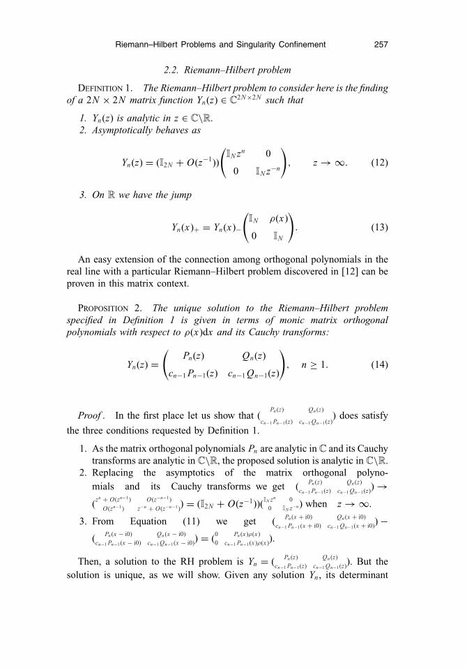
2.2. Riemann–Hilbert problem
DEFINITION 1. The Riemann–Hilbert problem to consider here is the findingof a 2N × 2N matrix function Yn(z) ∈ C
2N×2N such that
1. Yn(z) is analytic in z ∈ C\R.2. Asymptotically behaves as
Yn(z) = (I2N + O(z−1))
(IN zn 0
0 IN z−n
), z → ∞. (12)
3. On R we have the jump
Yn(x)+ = Yn(x)−
(IN ρ(x)
0 IN
). (13)
An easy extension of the connection among orthogonal polynomials in thereal line with a particular Riemann–Hilbert problem discovered in [12] can beproven in this matrix context.
PROPOSITION 2. The unique solution to the Riemann–Hilbert problemspecified in Definition 1 is given in terms of monic matrix orthogonalpolynomials with respect to ρ(x)dx and its Cauchy transforms:
Yn(z) =(
Pn(z) Qn(z)
cn−1 Pn−1(z) cn−1 Qn−1(z)
), n ≥ 1. (14)
Proof . In the first place let us show that (Pn (z) Qn (z)
cn−1 Pn−1(z) cn−1 Qn−1(z)) does satisfy
the three conditions requested by Definition 1.
1. As the matrix orthogonal polynomials Pn are analytic in C and its Cauchytransforms are analytic in C\R, the proposed solution is analytic in C\R.
2. Replacing the asymptotics of the matrix orthogonal polyno-mials and its Cauchy transforms we get ( Pn (z) Qn (z)
cn−1 Pn−1(z) cn−1 Qn−1(z)) →(zn + O(zn−1) O(z−n−1)
O(zn−1) z−n + O(z−n−1)) = (I2N + O(z−1))(IN zn 0
0 IN z−n) when z → ∞.
3. From Equation (11) we get ( Pn (x + i0) Qn (x + i0)cn−1 Pn−1(x + i0) cn−1 Qn−1(x + i0)) −
( Pn (x − i0) Qn (x − i0)cn−1 Pn−1(x − i0) cn−1 Qn−1(x − i0)) = (0 Pn (x)ρ(x)
0 cn−1 Pn−1(x)ρ(x)).
Then, a solution to the RH problem is Yn = ( Pn (z) Qn (z)cn−1 Pn−1(z) cn−1 Qn−1(z)). But the
solution is unique, as we will show. Given any solution Yn , its determinant

258 G. A. Cassatella-Contra and M. Manas
det Yn(z) is analytic in C\R and satisfies
detYn(x)+ = det
(Yn(x)−
(IN ρ(x)
0 IN
))= detYn(x)−det
(IN ρ(x)
0 IN
)
= detYn(x)−.
Hence, det Yn(z) is analytic in C. Moreover, Definition 1 implies that
detYn(z) = 1 + O(z−1), z → ∞,
and Liouville theorem ensures that
detYn(z) = 1, ∀z ∈ C. (15)
From Equation (15) we conclude that Y −1n is analytic in C\R. Given two
solutions Yn and Yn of the RH problem we consider the matrix YnY −1n , and
observe that from property 3 of Definition 1 we have (YnY −1n )+ = (YnY −1
n )−, andconsequently YnY −1
n is analytic in C. From Definition 1 we get YnY −1n → I2N
as z → ∞, and Liouville theorem implies that YnY −1n = I2N ; that is, Yn = Yn
and the solution is unique. �
DEFINITION 2. Given the matrix Yn we define
Sn(z) := Yn(z)
(IN z−n 0
0 IN zn
). (16)
PROPOSITION 3.
1. The matrix Sn has unit determinant:
detSn(z) = 1. (17)
2. It has the special form
Sn(z) =(
An(z2) z−1 Bn(z2)
z−1Cn(z2) Dn(z2)
). (18)
3. The coefficients of Sn admit the asymptotic expansions
An(z2) = IN + S(2)n,11z−2 + O(z−4), Bn(z2) = S(1)
n,12 + S(3)n,12z−2 + O(z−4),
Cn(z2) = S(1)n,21 + S(3)
n,21z−2 + O(z−4), Dn(z2) = IN + S(2)n,22z−2 + O(z−4),
for z → ∞. (19)
Proof .
1. Is a consequence of Equations (15) and (16).2. It follows from the parity of Pn and Qn .
Riemann–Hilbert Problems and Singularity Confinement 259
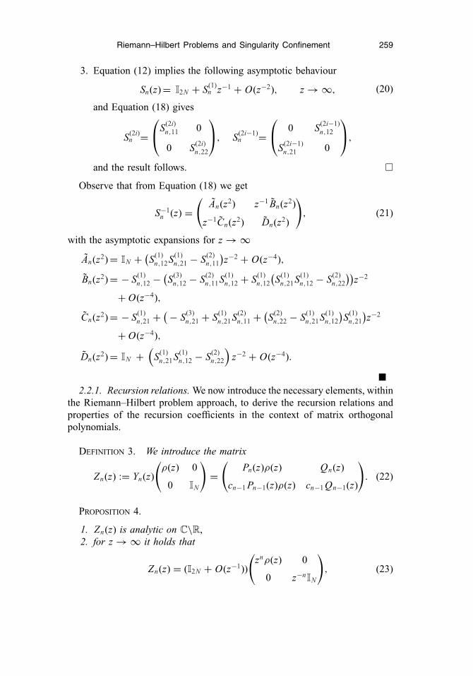
3. Equation (12) implies the following asymptotic behaviour
Sn(z) = I2N + S(1)n z−1 + O(z−2), z → ∞, (20)
and Equation (18) gives
S(2i)n =
⎛⎝S(2i)
n,11 0
0 S(2i)n,22
⎞⎠, S(2i−1)
n =⎛⎝ 0 S(2i−1)
n,12
S(2i−1)n,21 0
⎞⎠,
and the result follows. �Observe that from Equation (18) we get
S−1n (z) =
(An(z2) z−1 Bn(z2)
z−1Cn(z2) Dn(z2)
), (21)
with the asymptotic expansions for z → ∞An(z2) = IN + (
S(1)n,12S(1)
n,21 − S(2)n,11
)z−2 + O(z−4),
Bn(z2) = − S(1)n,12 − (
S(3)n,12 − S(2)
n,11S(1)n,12 + S(1)
n,12
(S(1)
n,21S(1)n,12 − S(2)
n,22
))z−2
+ O(z−4),
Cn(z2) = − S(1)n,21 + ( − S(3)
n,21 + S(1)n,21S(2)
n,11 + (S(2)
n,22 − S(1)n,21S(1)
n,12
)S(1)
n,21
)z−2
+ O(z−4),
Dn(z2) = IN +(
S(1)n,21S(1)
n,12 − S(2)n,22
)z−2 + O(z−4).
�2.2.1. Recursion relations. We now introduce the necessary elements, within
the Riemann–Hilbert problem approach, to derive the recursion relations andproperties of the recursion coefficients in the context of matrix orthogonalpolynomials.
DEFINITION 3. We introduce the matrix
Zn(z) := Yn(z)
(ρ(z) 0
0 IN
)=
(Pn(z)ρ(z) Qn(z)
cn−1 Pn−1(z)ρ(z) cn−1 Qn−1(z)
). (22)
PROPOSITION 4.
1. Zn(z) is analytic on C\R,2. for z → ∞ it holds that
Zn(z) = (I2N + O(z−1))
(znρ(z) 0
0 z−nIN
), (23)
260 G. A. Cassatella-Contra and M. Manas
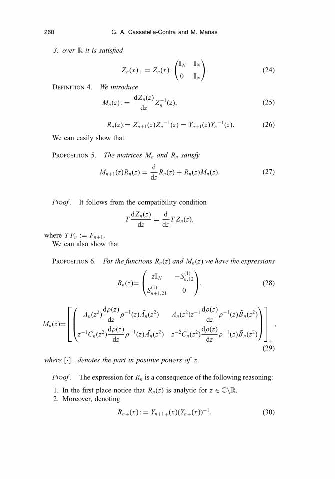
3. over R it is satisfied
Zn(x)+ = Zn(x)−
(IN IN
0 IN
). (24)
DEFINITION 4. We introduce
Mn(z) : = dZn(z)
dzZ−1
n (z), (25)
Rn(z):= Zn+1(z)Zn−1(z) = Yn+1(z)Yn
−1(z). (26)
We can easily show that
PROPOSITION 5. The matrices Mn and Rn satisfy
Mn+1(z)Rn(z) = d
dzRn(z) + Rn(z)Mn(z). (27)
Proof . It follows from the compatibility condition
TdZn(z)
dz= d
dzT Zn(z),
where T Fn := Fn+1.We can also show that
PROPOSITION 6. For the functions Rn(z) and Mn(z) we have the expressions
Rn(z)=⎛⎝ zIN −S(1)
n,12
S(1)n+1,21 0
⎞⎠, (28)
Mn(z)=
⎡⎢⎢⎣⎛⎜⎜⎝
An(z2)dρ(z)
dzρ−1(z) An(z2) An(z2)z−1 dρ(z)
dzρ−1(z)Bn(z2)
z−1Cn(z2)dρ(z)
dzρ−1(z) An(z2) z−2Cn(z2)
dρ(z)
dzρ−1(z)Bn(z2)
⎞⎟⎟⎠⎤⎥⎥⎦
+
,
(29)
where [·]+ denotes the part in positive powers of z.
Proof . The expression for Rn is a consequence of the following reasoning:
1. In the first place notice that Rn(z) is analytic for z ∈ C\R.2. Moreover, denoting
Rn+(x) : = Yn+1+(x)(Yn+(x))−1, (30)
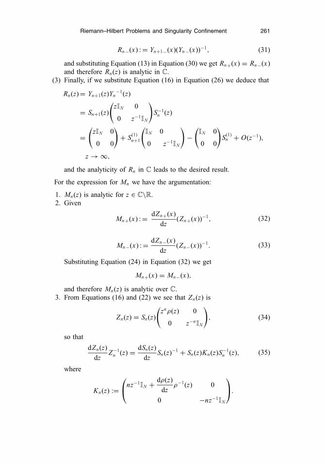
Riemann–Hilbert Problems and Singularity Confinement 261
Rn−(x) : = Yn+1−(x)(Yn−(x))−1, (31)
and substituting Equation (13) in Equation (30) we get Rn+(x) = Rn−(x)and therefore Rn(z) is analytic in C.
(3) Finally, if we substitute Equation (16) in Equation (26) we deduce that
Rn(z) = Yn+1(z)Yn−1(z)
= Sn+1(z)
(zIN 0
0 z−1IN
)S−1
n (z)
=(
zIN 0
0 0
)+ S(1)
n+1
(IN 0
0 z−1IN
)−
(IN 0
0 0
)S(1)
n + O(z−1),
z → ∞,
and the analyticity of Rn in C leads to the desired result.
For the expression for Mn we have the argumentation:
1. Mn(z) is analytic for z ∈ C\R.2. Given
Mn+(x) : = dZn+(x)
dz(Zn+(x))−1, (32)
Mn−(x) : = dZn−(x)
dz(Zn−(x))−1. (33)
Substituting Equation (24) in Equation (32) we get
Mn+(x) = Mn−(x),
and therefore Mn(z) is analytic over C.3. From Equations (16) and (22) we see that Zn(z) is
Zn(z) = Sn(z)
(znρ(z) 0
0 z−nIN
), (34)
so that
dZn(z)
dzZ−1
n (z) = dSn(z)
dzSn(z)−1 + Sn(z)Kn(z)S−1
n (z), (35)
where
Kn(z) :=⎛⎝nz−1
IN + dρ(z)
dzρ−1(z) 0
0 −nz−1IN
⎞⎠.

262 G. A. Cassatella-Contra and M. Manas
Finally, as Mn(z) is analytic over C, Equation (35) leads to
Mn(z) = dZn(z)
dzZ−1
n (z) =[
Sn(z)
⎛⎝dρ(z)
dzρ−1(z) 0
0 0
⎞⎠S−1
n (z)
]+. (36)
Observe that the diagonal terms of Mn are odd functions of z while the offdiagonal are even functions of z. Now we give a parametrization of the firstcoefficients of S in terms of cn . �
PROPOSITION 7. The following formulae hold true
S(1)n,12 = c−1
n , S(1)n,21 = cn−1,
S(2)n,11 = −
n∑i=1
c−1i ci−1 + c−1
n cn−1, S(2)n,22 =
n∑i=1
ci−1c−1i ,
S(3)n,21 = −cn−1
n−1∑i=1
c−1i ci−1 + cn−2, S(3)
n,12 = c−1n
n+1∑i=1
ci−1c−1i .
Proof . Equating the expressions for Yn(z) provided by Equation (14) andEquation (16) we get
Yn(z) =(
Pn(z) Qn(z)
cn−1 Pn−1(z) cn−1 Qn−1(z)
)
=(
znIN 0
0 z−nIN
)(I2N + S(1)
n z−1 + S(2)n z−2 + S(3)
n z−3 + O(z−4)),
z → ∞.
Expanding the right hand side we get
S(1)n,21 = cn−1, S(1)
n,12 = c−1n ,
S(2)1,11 = 0,
S(3)1,21 = S(3)
2,21 = 0, S(3)n,21 = cn−1S(2)
n−1,11, n ≥ 2,
S(3)n,12 = c−1
n S(2)n+1,22,
(37)
where we have used that
S(2)1,22 = c0c−1
1 , (38)

Riemann–Hilbert Problems and Singularity Confinement 263
which can be proved from Equation (10). Introducing Equation (37) intoEquation (28) we get
Rn(z) =(
zIN −c−1n
cn 0
), (39)
and Equations (16) and (39) lead to
Sn+1(z) =(
zIN −c−1n
cn 0
)Sn(z)
(z−1
IN 0
0 zIN
),
so that
S(2)n+1,11 − S(2)
n,11 = −c−1n cn−1, (40)
S(3)n,12 − c−1
n S(2)n,22 = c−1
n+1, (41)
where we have used Equation (37). From Equations (37) and (41) we get
S(2)n+1,22 − S(2)
n,22 = cnc−1n+1. (42)
Summing up in n in Equations (40) and (42) we deduce
n−1∑i=1
(S(2)
i+1,11 − S(2)i,11
)= −n−1∑i=1
c−1i ci−1,
n−1∑i=1
(S(2)
i+1,22 − S(2)i,22
)=n−1∑i=1
ci c−1i+1,
which leads to
S(2)n,11 = −
n∑i=1
c−1i ci−1 + c−1
n cn−1, (43)
S(2)n,22 =
n∑i=1
ci−1c−1i , (44)
where we have used Equations (37) and (38). Finally Equations (37), (43) and(44) give
S(3)n,21 = −cn−1
n−1∑i=1
c−1i ci−1 + cn−2, (45)
valid for n ≥ 2, and
S(3)n,12 = c−1
n
n+1∑i=1
ci−1c−1i . (46)

264 G. A. Cassatella-Contra and M. Manas
Notice that Equation (37) gives
S(3)1,21 = 0. (47)
�
PROPOSITION 8. Matrix orthogonal polynomials Pn (and its Cauchytransforms Qn) are subject to the following recursion relations
Pn+1(z) = z Pn(z) − 1
2βn Pn−1(z), (48)
with the recursion coefficients βn given by
βn : = 2c−1n cn−1, n ≥ 1, β0 := 0. (49)
Proof . Observe that Equation (26) can be written as
Yn+1(z) = Rn(z)Yn(z). (50)
Then, if we replace Equations (14) and (39) into Equation (50) we get the result.We now show some commutative properties of the polynomials and the
recursion coefficients. �
PROPOSITION 9. Let f (z) : C → CN×N such that [V (x), f (z)] = 0
∀(x, z) ∈ R × C, then
[cn, f (z)] = [βn, f (z)] = 0, n ≥ 0, ∀z ∈ C,
[Pn(z′), f (z)] = 0, n ≥ 0, ∀z, z′ ∈ C.
Proof . Let us suppose that for a given m ≥ 0 we have
[Pm(x), f (z)] = [Pm−1(x), f (z)] = 0. (51)
Then, recalling Equation (7) these expressions give
[cm, f (z)] = [cm−1, f (z)] = 0, (52)
respectively. Therefore, using the recursion relations Equations (48) and (49)we obtain
[Pm+1(x), f (z)] = x[Pm(x), f (z)] − [c−1
m cm−1 Pm−1(x), f (z)] = 0.
This means that
[cm+1, f (z)] = 0. (53)
Hypothesis Equation (51) holds for m = 1, consequently [cn, f (z)] = 0for n = 0, 1, . . . and Equation (49) implies [βn, f (z)] = 0. Finally, as the

Riemann–Hilbert Problems and Singularity Confinement 265
coefficients of the matrix orthogonal Pn(z) are polynomials in the β’s weconclude that [Pn(z′), f (z)] = 0 for all z, z′ ∈ C. �
COROLLARY 1. Suppose that [V (x), V (z)] = 0 for all x ∈ R and z ∈ C,then
[Pn(z), Pm(z′)] = 0, ∀n, m ≥ 0, z, z′ ∈ C, (54)
[cn, cm] = 0, (55)
[βn, βm]= 0. (56)
Proof . Applying Proposition 9 to f = V we deduce that [Pn(z′), V (z)]= 0, so that it allows to use again Proposition 9 but now with f = Pn and getthe stated result. From Equations (7) and (54) we deduce Equations (55) andusing Equation (49) we get Equation (56). �
3. A discrete matrix equation, related to Freud matrix orthogonalpolynomials, with singularity confinement
We will consider the particular case when
V (z) = αz2 + IN z4, α = α†. (57)
Observe that [V (z), V (z′)] = 0 for any pair of complex numbers z, z′. Hence,in this case the corresponding set of MOP {Pn}∞n=0, that we refer as matrixFreud polynomials, is an Abelian set. Moreover, we have
[cn, cm] = [βn, βm] = [cn, α] = [βn, α] = 0, ∀n, m = 0, 1, . . . .
In this situation, we have
THEOREM 1. The recursion coefficients βn Equation (49) for the Freudmatrix orthogonal polynomials determined by Equation (57) satisfy
βn+1 = nβ−1n − βn−1 − βn − α, n = 1, 2, . . . , (58)
with β0 := 0.
Proof . We compute now the matrix Mn , for which we have
Mn(z) =[(−An(z2)
(2αz + 4z3
IN
)An(z2) −An(z2)
(2α + 4z2
IN
)Bn(z2)
− Cn(z2)(2α + 4z2
IN
)An(z2) −Cn(z2)
(2αz−1 + 4zIN
)Bn(z2)
)]+,
(59)

266 G. A. Cassatella-Contra and M. Manas
and is clear that
Mn(z) = M (3)n z3 + M (2)
n z2 + M (1)n z + M (0)
n , (60)
with
M (3)n =
(−4IN 0
0 0
), M (2)
n =⎛⎝ 0 4S(1)
n,12
−4S(1)n,21 0
⎞⎠,
M (1)n =
⎛⎝−2α − 4S(1)
n,12S(1)n,21 0
0 4S(1)n,21S(1)
n,12
⎞⎠,
M (0)n =
⎛⎜⎜⎜⎜⎜⎜⎝
02αS(1)
n,12 + 4S(3)n,12
+ 4S(1)n,12
(S(1)
n,21S(1)n,12 − S(2)
n,22
)−2S(1)
n,21α − 4S(3)n,21
+ 4S(1)n,21S(2)
n,11 − 4S(1)n,21S(1)
n,12S(1)n,21
0
⎞⎟⎟⎟⎟⎟⎟⎠
.
Replacing Equations (37)–(46) into Equation (60) we get
M (3)n =
(−4IN 0
0 0
), M (2)
n =(
0 4c−1n
−4cn−1 0
),
M (1)n =
(−2α − 4c−1n cn−1 0
0 4cn−1c−1n
),
(61)
M (0)1 =
(0 4c−1
2 + 4c−11 c0c−1
1 + 2αc−11
−4c0c−11 c0 − 2c0α 0
), (62)
M (0)n =
(0 4c−1
n+1 + 4c−1n cn−1c−1
n + 2αc−1n
−4cn−2 − 4cn−1c−1n cn−1 − 2cn−1α 0
),
n ≥ 2. (63)
The compatibility condition Equation (27) together with Equations (39) and(60)–(63) gives
4(c−1
n+2cn + c−1n+1cnc−1
n+1cn − c−1n cn−1c−1
n cn−1 − c−1n cn−2
) + 2αc−1n+1cn
− 2c−1n cn−1α = IN ,

Riemann–Hilbert Problems and Singularity Confinement 267
for n ≥ 2 and
4(c−1
3 c1 + c−12 c1c−1
2 c1 − c−11 c0c−1
1 c0) + 2αc−1
2 c1 − 2c−11 c0α = IN ,
which can be written as
βn+2βn+1 + β2n+1 − β2
n − βnβn−1 + αβn+1 − βnα = IN (64)
for n ≥ 2 and
β3β2 + β22 − β2
1 + αβ2 − β1α = IN , (65)
respectively. Using the Abelian character of the set of β’s we arrive to
βn+2βn+1 + β2n+1 − β2
n − βnβn−1 + α(βn+1 − βn) = IN , n=2, 3, . . . ,(66)
β3β2 + β22 − β2
1 + α(β2 − β1) = IN . (67)
Summing up in Equation (66) from i = 2 up to i = n we obtainn∑
i=2
[βi+2βi+1 + β2
i+1 − β2i − βiβi−1 + α(βi+1 − βi )
] =n∑
i=2
IN , (68)
and consequently we conclude that
βn+2βn+1 + βn+1βn + βn+12 + αβn+1 = nIN + k, n ≥ 1, (69)
where
k := β2β1 + β3β2 + β22 + αβ2 − IN = β2β1 + β2
1 + β1α, (70)
where we have used Equation (67). We now proceed to show that k = IN .Equation (25) implies, for n = 1 and z = 0,
Z ′1(0) = M (0)
1 Z1(0), (71)
with M (0)1 given in Equation (62). This leads to(
P ′1(0)
c0 P ′0(0)
)= M (0)
1
(P1(0)
c0 P0(0)
). (72)
Now, using Equation (3) we deduce that(IN
0
)= M (0)
1
(0
c0
), (73)
which allows us to immediately deduce that
β2β1 + β21 + β1α = IN , (74)
and consequently k = IN . Finally, we get
βn+2βn+1 + βn+1βn + βn+12 + αβn+1 = nIN + IN . (75)
268 G. A. Cassatella-Contra and M. Manas
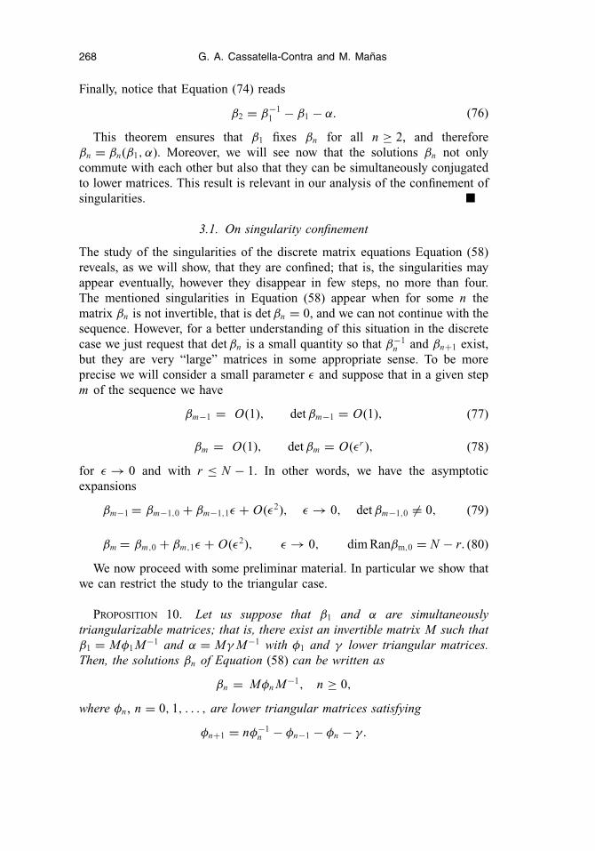
Finally, notice that Equation (74) reads
β2 = β−11 − β1 − α. (76)
This theorem ensures that β1 fixes βn for all n ≥ 2, and thereforeβn = βn(β1, α). Moreover, we will see now that the solutions βn not onlycommute with each other but also that they can be simultaneously conjugatedto lower matrices. This result is relevant in our analysis of the confinement ofsingularities. �
3.1. On singularity confinement
The study of the singularities of the discrete matrix equations Equation (58)reveals, as we will show, that they are confined; that is, the singularities mayappear eventually, however they disappear in few steps, no more than four.The mentioned singularities in Equation (58) appear when for some n thematrix βn is not invertible, that is det βn = 0, and we can not continue with thesequence. However, for a better understanding of this situation in the discretecase we just request that det βn is a small quantity so that β−1
n and βn+1 exist,but they are very “large” matrices in some appropriate sense. To be moreprecise we will consider a small parameter ε and suppose that in a given stepm of the sequence we have
βm−1 = O(1), det βm−1 = O(1), (77)
βm = O(1), det βm = O(εr ), (78)
for ε → 0 and with r ≤ N − 1. In other words, we have the asymptoticexpansions
βm−1 = βm−1,0 + βm−1,1ε + O(ε2), ε → 0, det βm−1,0 �= 0, (79)
βm = βm,0 + βm,1ε + O(ε2), ε → 0, dim Ranβm,0 = N − r. (80)
We now proceed with some preliminar material. In particular we show thatwe can restrict the study to the triangular case.
PROPOSITION 10. Let us suppose that β1 and α are simultaneouslytriangularizable matrices; that is, there exist an invertible matrix M such thatβ1 = Mφ1 M−1 and α = Mγ M−1 with φ1 and γ lower triangular matrices.Then, the solutions βn of Equation (58) can be written as
βn = Mφn M−1, n ≥ 0,
where φn , n = 0, 1, . . . , are lower triangular matrices satisfying
φn+1 = nφ−1n − φn−1 − φn − γ.
Riemann–Hilbert Problems and Singularity Confinement 269
Moreover, let us suppose that for some integer m the matrices βm+1, βm
and α are simultaneously triangularizable, then all the sequence {βn}∞n=0 issimultaneously triangularizable.
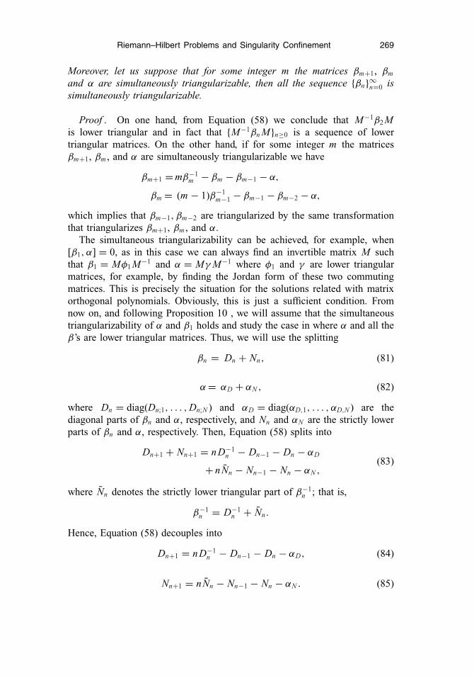
Proof . On one hand, from Equation (58) we conclude that M−1β2 Mis lower triangular and in fact that {M−1βn M}n≥0 is a sequence of lowertriangular matrices. On the other hand, if for some integer m the matricesβm+1, βm , and α are simultaneously triangularizable we have
βm+1 = mβ−1m − βm − βm−1 − α,
βm = (m − 1)β−1m−1 − βm−1 − βm−2 − α,
which implies that βm−1, βm−2 are triangularized by the same transformationthat triangularizes βm+1, βm , and α.
The simultaneous triangularizability can be achieved, for example, when[β1, α] = 0, as in this case we can always find an invertible matrix M suchthat β1 = Mφ1 M−1 and α = Mγ M−1 where φ1 and γ are lower triangularmatrices, for example, by finding the Jordan form of these two commutingmatrices. This is precisely the situation for the solutions related with matrixorthogonal polynomials. Obviously, this is just a sufficient condition. Fromnow on, and following Proposition 10 , we will assume that the simultaneoustriangularizability of α and β1 holds and study the case in where α and all theβ’s are lower triangular matrices. Thus, we will use the splitting
βn = Dn + Nn, (81)
α = αD + αN , (82)
where Dn = diag(Dn;1, . . . , Dn;N ) and αD = diag(αD,1, . . . , αD,N ) are thediagonal parts of βn and α, respectively, and Nn and αN are the strictly lowerparts of βn and α, respectively. Then, Equation (58) splits into
Dn+1 + Nn+1 = nD−1n − Dn−1 − Dn − αD
+ nNn − Nn−1 − Nn − αN ,(83)
where Nn denotes the strictly lower triangular part of β−1n ; that is,
β−1n = D−1
n + Nn.
Hence, Equation (58) decouples into
Dn+1 = nD−1n − Dn−1 − Dn − αD, (84)
Nn+1 = nNn − Nn−1 − Nn − αN . (85)
270 G. A. Cassatella-Contra and M. Manas
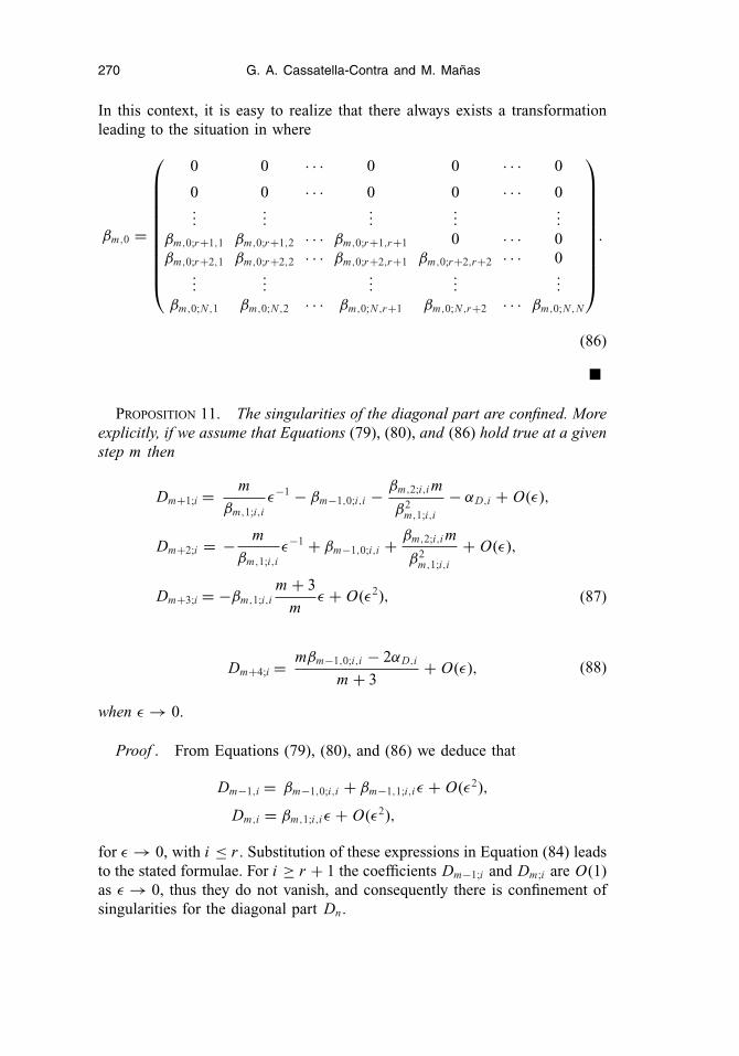
In this context, it is easy to realize that there always exists a transformationleading to the situation in where
βm,0 =
⎛⎜⎜⎜⎜⎜⎜⎜⎜⎜⎜⎝
0 0 · · · 0 0 · · · 0
0 0 · · · 0 0 · · · 0...
......
......
βm,0;r+1,1 βm,0;r+1,2 · · · βm,0;r+1,r+1 0 · · · 0βm,0;r+2,1 βm,0;r+2,2 · · · βm,0;r+2,r+1 βm,0;r+2,r+2 · · · 0
......
......
...βm,0;N ,1 βm,0;N ,2 · · · βm,0;N ,r+1 βm,0;N ,r+2 · · · βm,0;N ,N
⎞⎟⎟⎟⎟⎟⎟⎟⎟⎟⎟⎠
.
(86)
�
PROPOSITION 11. The singularities of the diagonal part are confined. Moreexplicitly, if we assume that Equations (79), (80), and (86) hold true at a givenstep m then
Dm+1;i = m
βm,1;i,iε−1 − βm−1,0;i,i − βm,2;i,i m
β2m,1;i,i
− αD,i + O(ε),
Dm+2;i = − m
βm,1;i,iε−1 + βm−1,0;i,i + βm,2;i,i m
β2m,1;i,i
+ O(ε),
Dm+3;i = −βm,1;i,im + 3
mε + O(ε2), (87)
Dm+4;i = mβm−1,0;i,i − 2αD,i
m + 3+ O(ε), (88)
when ε → 0.
Proof . From Equations (79), (80), and (86) we deduce that
Dm−1,i = βm−1,0;i,i + βm−1,1;i,iε + O(ε2),
Dm,i = βm,1;i,iε + O(ε2),
for ε → 0, with i ≤ r . Substitution of these expressions in Equation (84) leadsto the stated formulae. For i ≥ r + 1 the coefficients Dm−1;i and Dm;i are O(1)as ε → 0, thus they do not vanish, and consequently there is confinement ofsingularities for the diagonal part Dn .

Riemann–Hilbert Problems and Singularity Confinement 271
In what follows we will consider asymptotic expansions taking values in theset of lower triangular matrices
T : ={T0 + T1ε + O(ε2), ε → 0, Ti ∈ tN }, tN := {T = (Ti, j ) ∈ CN×N ,
Xi, j = 0 when i > j}, (89)
where tN is the set of lower triangular N × N matrices. The reader shouldnotice that this set T = tN [[ε]] is a subring of the ring of C
N×N -valuedasymptotic expansions; in fact is a subring with identity, the matrix IN . Wewill use the notation
Ti : =(
Ti,11 0
Ti,21 Ti,22
), i ≥ 1, (90)
where Ti,11 ∈ tr , Ti,22 ∈ tN−r , and Ti,21 ∈ C(N−r )×r . We consider two sets of
matrices determined by Equation (86), namely
k : ={
K0 =(
0 0
K0,21 K0,22
), K0,21 ∈ C
(N−r )×r , K0,22 ∈ tN−r
},
l := {L−1 =(
L−1,11 0
L−1,21 0
), L−1,11 ∈ tr , L−1,21 ∈ C
(N−r )×r},
and the related sets
K : = {K = K0 + K1ε + O(ε2) ∈ T, K0 ∈ k
}, (91)
L : = {L = L−1ε
−1 + L0 + L1ε + O(ε2) ∈ ε−1T, L−1 ∈ l
}, (92)
which fulfill the following important properties. �
PROPOSITION 12.
1. Both K and εL are subrings of the ring with identity T, however thesetwo subrings have no identity.
2. If an element X ∈ K with r = r0 is such that det X = O(εr0 ) for ε → 0,then X−1 ∈ L, and reciprocally if X ∈ L with r = r0 is such thatdet X = O(ε−r0 ) for ε → 0, then X−1 ∈ K.
3. The subrings εL and K are bilateral ideals of T; that is, L · T ⊂ L,T · L ⊂ L, T · K ⊂ K, and K · T ⊂ K.
4. We have L · K ⊂ T.
THEOREM 2. If β1 and α are simultaneously triangularizable matrices thenthe singularities of Equation (58) are confined. More explicitly, if for a givenstep m the conditions Equations (79), (80) and (86) are satisfied then
βm+1, βm+2∈ L, βm+3 ∈ K, βm+4 ∈ T, det βm+4 = O(1), ε → 0.

272 G. A. Cassatella-Contra and M. Manas
Proof . From Equations (80) and (86) we conclude that βm ∈ K andconsequently β−1
m ∈ L. Taking into account this fact, Equation (58) impliesthat βm+1 ∈ L. Therefore, β−1
m+1 ∈ K and Equation (58), as βm+1 ∈ L, giveβm+2 ∈ L and consequently β−1
m+2 ∈ K. Iterating Equation (58) we get
βm+3 = βm − (m + 1)β−1m+1 + (m + 2)β−1
m+2. (93)
Using the just derived facts, β−1m+1, β
−1m+2 ∈ K, and that βm ∈ K, we deduce
βm+3 ∈ K which implies β−1m+3 ∈ L. Finally, Equation (58) gives βm+4 as
βm+4 = (m + 3)β−1m+3 − βm+2 − βm+3 − α. (94)
We conclude that there are only two possibilities:
1. βm+4 = O(1) for ε → 0, or2. βm+4 ∈ L.
Let us consider both possibilities separately.
1. Recalling that the diagonal part has singularity confinement, seeProposition 11, in the first case we see that det βm+4 = O(1) whenε → 0, as desired.
2. In this second case we write βm+4 as
βm+4 = β−1m+3 A + O(1), ε → 0, A := (m + 3)I − βm+3βm+2. (95)
Observe that the repeated use of Equation (58) leads to the followingexpressions:
A = I + [(m + 1)β−1
m+1 − βm
]βm+2
= k + I − [(m + 1)β−1
m+1 − βm
]βm+1
= k − mI + βmβm+1
= k − βm(βm + βm−1 + α),
where
k := [(m + 1)β−1
m+1 − βm
][(m + 1)β−1
m+1 − βm − α].
From these formulae, as β−1m+1, βm ∈ K we deduce that k ∈ K and also
that βm(βm + βm−1 + α) ∈ K. Hence, we conclude that A ∈ K and fromEquation (95) and Proposition 12 we deduce that βm+4 = O(1) whenε → 0. Consequently, we arrive to a contradiction, and only possibility1) remains. �

Riemann–Hilbert Problems and Singularity Confinement 273
Acknowledgments
The authors thanks economical support from the Spanish Ministerio de Cienciae Innovacion, research project FIS2008-00200. GAC acknowledges the supportof the grant Universidad Complutense de Madrid. Finally, MM reckonsilluminating discussions with Dr. Mattia Cafasso in relation with orthogonalityand singularity confinement, and both authors are grateful to Prof. GabrielAlvarez Galindo for several discussions and for the experimental confirmation,via MATHEMATICA, of the existence of the confinement of singularities in the2 × 2 case.
References
1. P. PAINLEVE, LECONS sur la theorie analytique des equations differentielles (Lecons deStockholm, delivered in 1895), Hermann, Paris, 1897. Reprinted in Œvres de PaulPainleve, vol. I, Editions du CNRS, Paris, 1973.
2. R. CONTE (Ed.), The Painleve Property, One Century Later, Springer Verlag, New York,1999.
3. B. GRAMMATICOS, A. RAMANI, and V. PAPAGEORGIOU, Do integrable mappings have thePainleve property? Phys. Rev. Lett. 67:1825–1828 (1991).
4. B. GRAMMATICOS, A. RAMANI, and J. HIETARINTA, Discrete versions of the Painleveequations, Phys. Rev. Lett. 67:1829–1832 (1991).
5. A. RAMANI, D. TAKAHASHI, B. GRAMMATICOS, and Y. OHTA, The ultimate discretisationof the Painleve equations, Physica D 114:185–196 (1998).
6. J. HIETARINTA and C. VIALLET, Discrete Painleve I and singularity confinement inprojective space, Chaos, Solitons and Fractals 11:29–32 (2000).
7. S. LAFORTUNE and A. GORIELY, Singularity confinement and algebraic integrability, J.Math. Phys. 45:1191–1208 (2004).
8. G. FREUD, On the coefficients in the recursion formulae of orthogonal polynomials,Proc. R. Irish Acad. A76:1–6 (1976).
9. W. VAN ASSCHE, Discrete Painleve equations for recurrence coefficients of orthogonalpolynomials, in Proceedings of the International Conference on Difference Equations,special Functions and Orthogonal Polynomials, pp. 687–725, World Scientific, Hackensack,NJ (2007).
10. A. P. MAGNUS, Freud’s equations for orthogonal polynomials as discrete Painleveequations, in Symmetries and Integrability of Difference Equations (Canterbury, 1996),London Math. Soc. Lecture Note Ser., 255, pp. 228–243, Cambridge University PressCambridge, UK (1999).
11. D. DAMANIK, A. PUSHNITSKI, and B. SIMON, The analytic theory of matrix orthogonalpolynomials, Surv. Approx. Theory 4:1–85 (2008).
12. A. S. FOKAS, A. R. ITS, and A. V. KITAEV, The isomonodromy approach to matrixmodels in 2D quantum gravity, Commun. Math. Phys. 147:395–430 (1992).
13. E. DAEMS and A. B. J. KUIJLAARS, Multiple orthogonal polynomials of mixed type andnon-intersecting Brownian motions, J. Approx. Theory 146:91–114 (2007).
14. M. G. KREIN, Infinite J-matrices and a matrix moment problem, Dokl. Akad. Nauk. SSSR69:125–128 (1949).
274 G. A. Cassatella-Contra and M. Manas
15. M. G. KREIN, Fundamental Aspects of the Representation Theory of Hermitian Operatorswith Deficiency Index (m,m), AMS Translations, Series 2, Vol. 97, pp. 75–143, Providence,Rhode Island, 1971.
16. YU. M. BEREZANSKII, Expansions in eigenfunctions of self-adjoint operators, Transl.Math. Monographs 17, Amer. Math. Soc. Providence, RI, 1968.
17. J. S. GERONIMO, Scattering theory and matrix orthogonal polynomials on the real line,Circ. Syst. Sig. Proc. 1:471–495 (1982).
18. A. I. APTEKAREV and E. M. NIKISHIN, The scattering problem for a discrete Sturm–Liouvilleoperator, Math. USSR-Sb. 49:325–355 (1984).
19. A. J. DURAN and F. J. GRUNBAUM, Orthogonal matrix polynomials, scalar-type Rodrigues’formulas and Pearson equations, J. Approx. Theory 134:267–280 (2005).
20. A. J. DURAN and F. J. GRUNBAUM, Structural formulas for orthogonal matrix polynomialssatisfying second order differential equations, I, Constr. Approx. 22:255–271 (2005).
21. R. D. COSTIN, Matrix valued polynomials generated by the scalar-type Rodrigues’formulas, J. Approx. Theory 161:693–705 (2009).
22. A. J. DURAN, Matrix inner product having a matrix symmetric second order differentialoperator, Rocky Mount. J. Math. 27:585–600 (1997).
23. A. J. DURAN and F. J. GRUNBAUM, Orthogonal matrix polynomials satisfying secondorder differential equations, Int. Math. Res. Notices 10:461–484 (2004).
24. J. BORREGO, M. CASTRO, and A. J. DURAN, Orthogonal matrix polynomials satisfyingdifferential equations with recurrence coefficients having non-scalar limits, IntegralTransforms and Special Functions 1–16 (2011).
25. A. J. DURAN and M. D. DE LA IGLESIA, Second order differential operators havingseveral families of orthogonal matrix polynomials as eigenfunctions, Int. Math. Res.Not., Article ID rnn084, 24 p. (2008).
26. M. J. CANTERO, L. MORAL, and L. VELAZQUEZ, Differential properties of matrix orthogonalpolynomials, J. Concrete Appl. Math. 3:313–334 (2005).
UNIVERSIDAD COMPLUTENSE DE MADRID
(Received June 14, 2011)

Copyright of Studies in Applied Mathematics is the property of Wiley-Blackwell and its content may not be
copied or emailed to multiple sites or posted to a listserv without the copyright holder's express written
permission. However, users may print, download, or email articles for individual use.
Copyright © 2022 FDOKUMEN