Singularity analysis of planar parallel manipulators

Pergamon Mech. Math. Theory Vol. 30, No. 5, pp. 665-678, 1995

Copyright © 1995 Elsevier Science Ltd 0094-114X(94)00071-9 Printed in Great Britain. All rights reserved

0094-114X/95 $9.50 + 0.00

SINGULARITY ANALYSIS OF PLANAR PARALLEL MANIPULATORS

H. R. MOHAMMADI DANIALI, P. J. ZSOMBOR-MURRAY and J. ANGELES McGill Centre for Intelligent Machines & Department of Mechanical Engineering, McGill University,

817 Sherbrooke Street West, Montreal, Canada H3A 2K6

(Received 3 January 1994; in revised form 22 August 1994; received for publication 7 December 1994)

Abstract--With regard to planar parallel-manipulators, a general classification of singularities into three groups is introduced. The classification scheme relies on the properties of the Jacobian matrices of the manipulator at hand. The Jacobian matrices of two classes of planar parallel manipulators are derived and the three types of singularities are identified for them. The first class contains 20 manipulators constructed with three different combinations of legs of the PRR, PPR, RRR and RPR types, P and R representing prismatic and revolute pairs, respectively. The second class consists of 4 manipulators constructed with three legs of the PRP and RRP types. Finally, one example for each class is included. Contrary to earlier claims, we show that the third type of singularity is not necessarily architecture- dependent.

1, I N T R O D U C T I O N

For many years the positioning accuracy of manipulators has been a major concern. Accuracy can be characterized using some properties of the associated Jacobian matrices. Germane to accuracy is the concept of singularity, which has been extensively studied in the realm of serial manipulators [1-8], but less so with regard to manipulators having kinematic loops, where work is rather recent [9-13].

In [10], a classification of the singularities pertaining to manipulators with kinematic loops was suggested. This classification is based on the singularities of the two Jacobian matrices that relate the input rates with the Cartesian speeds. However, this classification is formulation- dependent, an analysis of purely kinematic singularities remaining as yet to be reported. In I11], another classification of singularities into three groups was given, namely, formulation singularities, configuration singularities and architecture singularities. To the authors' knowledge, no other classification of singularities for general kinematic chains with multiple loops has been reported in the literature, which motivated the research work presented in this paper.

A general class of planar parallel manipulator consists of two elements, namely the base (:~) and moving (~t') plates, connected by three legs, Fig. 1. The degree of freedom (dof) 1 of the manipulator is determined by means of the Chebyshev-Griibler-Kutzbach formula, namely,

l = 3(n - 1) - 2p (1)

where n and p are, respectively, the numbers of links and elementary revolute (R) or prismatic (P) pairs.

For the manipulator of Fig. 1 we have n = 8 and p = 9, and hence, the dof of the manipulator is

l = 3 × 7 - 2 x 9 = 3 (2)

We can build several 3-dof manipulators with three legs, each leg containing three elementary pairs. These legs are PRR, PRP, PPR, RRR, RRP, RPR and RPP. Since we can choose to actuate any one of three joints of the legs, we have 3 x 7 = 21 different legs and actuation modes. It is convenient, however, to actuate the joints attached to ~ , in order to have stationary motor frames, our choice then becoming limited to seven types of legs and actuation modes. Moreover, we cannot have a full 3-dof device with more than one leg of the RPP type for the whole manipulator.

665

666 H. R. Mohammadi Daniali et al.

le9 1

Fig. 1. The graph of general 3-dof, 3L parallel manipulator.

Let us classify the legs into two categories, based on their third joint. Those legs attached to J / with a revolute joint form the first category, i.e., PRR, PPR, RRR and RPR. We can choose any three combinations of the four legs in which the order of choice is not important. Then, we can build a variety of 3-legged (3L) parallel manipulators with these legs. Let us call these manipulators of class sg. The number in this class is given by

4

n = ~ ( 4 - i + 1 ) i = 2 0 i = 1

Those legs attached to ~ /w i th a prismatic joint form the legs of another 3L parallel manipulator class that will be called class 8 . The joint sequences for the legs are PRP and RRP. Similarly, we can choose any combination of three of these two leg types in which the order of choice is not important. We can thus build

2

n = ~ ( 2 - - i + 1 ) i = 4 i = 1

different manipulators with these legs. Here, we review the classifications of singularities, suggested in [10], encountered in parallel

manipulators and propose an alternative classification into three main types. The three types of singularities will be illustrated for the two classes of manipulators defined above. One example for each class of manipulators is given, and its three types of singularities are identified.

2. JACOBIAN MATRICES

In planar mechanisms, the relationship between actuator coordinates, grouped in the 3-dimensional vector 0, and Cartesian coordinates, grouped in the 3-dimensional vector x, can be written in general as:

f(0, x) = 0 (3)

where f is a 3-dimensional vector function of 0 and x, while 0 is the 3-dimensional zero vector. The underlying differential kinematic relations, in turn, take on the form

J0 + Kt = 0 (4)

where J and K are the two 3 × 3 Jacobian matrices of the manipulator at hand. Moreover, t is the 3-dimensional twist or Cartesian-velocity vector, and 0 is the 3-dimensional joint-velocity vector, defined below as

Of J - (5)

O0

Of K = (6)

dx

Furthermore, co is the scalar angular velocity and ~: is the 2-dimensional velocity vector of the operation point of ~g, respectively.

Singularity analysis of planar parallel manipulators 667

Mi

B i

Fig. 2. The ith leg of a parallel manipulator of class d .

Below we derive expressions for J and K for the two classes of planar manipulators introduced in Section 1.

2.1. Manipulators of class ~¢

In this subsection we will derive the Jacobian matrices of the 20 different manipulators of class d discussed in Section 1. The leg of the manipulator, in general, is depicted in Fig. 2, in which M~ represents the ith motor and C is the operation point of ~ ' . Moreover, joint B~ is a revolute, while joints Mr,. and Ai can be either revolute or prismatic.

The velocity ~ can be written for the ith leg as

= i, + (b, - ~i,) + (~ - b,) (8)

where a~ and b~ are the position vectors of points A~ and B~, respectively. Moreover, we have

ai = 0/El qi (9)

where 0~ is the rate of the ith actuator, q~ is the vector directed from M~ to Ai and E, is defined as

E, if the first joint is revolute

E, = (1/llq~ll)l, if the first joint is prismatic (10)

in which 1 is the 2 x 2 identity matrix and E is the 2 x 2 orthogonal matrix rotating vectors in a plane through an angle of 90 ° counterclockwise, i.e.,

Moreover, we have

b i - ai = }iE:ri + (~iE3ri (11)

where ~ is the rate of the second joint, ri is the vector directed from A~ to B~ and E2 and E3 are defined as

E, if the second joint is revolute E2 = (1/[J r i jr)l, if the second joint is prismatic

E, if the first joint is revolute Es = O, if the first joint is prismatic

(12)

(13)

668 H.R. Mohammadi Daniali et al.

Furthermore, ~ - I~i is given as

- 6i = ~ Esi (14)

with vector s~ directed from B~ to C, as shown in Fig: 2. Substitution of the values of ii, I~ i -ti~ and 6 - b ~ from equations (9), (11) and (14) into

equation (8), and simplification of the expression thus resulting leads to

0iEt q~ + ¢iE2ri + O~E3ri + oJEsi -- ~: --- 0 (15)

where ¢~, being associated with an unactuated joint, should be eliminated. This can be done by multiplication of the above equation by r~rE4, namely,

0~r[E4(Elq~ + E3ri) + cor~rE4Es~- r~rE4 ~ = 0 (16)

in which E4 is given as

1, if the second joint is revolute E4 ~ E, if the second joint is prismatic

Upon writing equation (16) for i = 1, 2, 3, we obtain

Jti + Kt = 0

where t, the twist vector, was defined above, and the 3 x 3 matrices J and K are given as

rTE4(E , q, + E3rt ) 0 0

J = 0 r2TE4(EIq2 + E3r2) 0

0 0 rTE4(Eiq3 + E3r3)

and

(17)

(18)

(19)

K = | r ] E 4 E s 2 - r2rE,/ (20) Lr~E4Es3 - r~E4J

in which EL, E2, E3 and E4 are chosen for each row of the foregoing matrices, separately, based on the corresponding leg, as explained in equations (10), (12), (13) and (17).

fi,

qi

Ai

ei M Fig. 3. The ith leg of a parallel manipulator of class at.


2.2. Manipulators of class In this subsection we will derive the Jacobian matrices of the 4 different manipulators of class discussed in Section 1. The leg of the manipulator, in general, is depicted in Fig. 3, in which

M/ represents the ith motor, fixed to the ground, and C is the operation point of ~¢ of the manipulator at hand. Moreover, A/is a revolute joint, Be is a prismatic joint and Mi can be either a revolute or a prismatic joint.

The velocity 4 can be now written for the ith leg as

6 = ~i/+ ( b , - ~ii) + (4 - I~,) (21)

where a~ and b~ are the position vectors of points di and B e, respectively. Moreover, we have

where Oi is the rate of the ith actuator and e~

{ E, ~ (1/lle,[I)l,

Moreover, we have

l~i- ae = coEqe

where ~/is the rate of the second joint and q/is the vector directed from Ae to B/. Furthermore, 6 - I~ e is given as

4 - I~, = )~/f/+ co Esi

hi = 0iEI ei (22)

is the vector directed from M~ to Ai and E1 is defined as

if the first joint is revolute (23) if the first joint is prismatic

(24)

(25)

with )~/denoting the rate of the third joint, f~ is a unit vector that represents the direction of the third joint, which is prismatic, and si is the vector directed from Bi to C, as shown in Fig. 3.

Substitution of the values of fi/, I~i- li/ and 4 i - l~i from equations (22), (24) and (25) into equation (21) and simplification of the expression thus resulting leads to

0iE, e~ + 2/fi + co E(qe + se) - 4 = 0 (26)

where ~/, being associated with an unactuated joint, should be eliminated. This can be done by multiplication of the above equation by f~E, namely,

0,f~EE~ e, - ~o fir(qi + si) - fTEe = 0

Upon writing equation (27) for i = 1, 2, 3, we obtain

J/~ + Kt = 0

where matrices J and K are given as

-f~EEi el

J = 0

0

and

K =

o o] f~ EEl e2 0

0 f3rEEi e 3

- - ftr(q, + sl) -- fTE] - f2T(q2 + S2) - f~ E /

- f3T(q3 + S3) -- f~E[

(27)

(28)

(29)

(30)

in which El is chosen for each row of J, separately, based on the corresponding leg, as explained in equation (23).

3. SINGULARITY ANALYSIS

In parallel manipulators, singularities occur whenever J, K or both become singular. Thus, for these manipulators, a distinction can be made between three types of singularities, which have different kinematic interpretations, namely:


(1) The first type of singularity occurs when ] becomes singular but K is invertible, i.e., when

det(J) = 0 and det(K) ~: 0 (31)

This type of singularity consists of the set of points where at least two branches of the inverse kinematic problem meet, this problem being understood here as the computation of the values of the driving-joint variables from given values of the Cartesian variables. Since the nullity of J is not zero, we can find a set of non-zero actuator velocity vectors 0 for which the Cartesian velocity vector t is zero. Then, nonzero Cartesian velocity vectors Kt, those lying in the nullspace of JX, cannot be produced, the manipulator thus losing one or more degrees of freedom at a first-order approximation.

(2) The second type of singularity, occurring only in closed kinematic chains, arises when K becomes singular but J is invertible, i.e., when

det(J) :/: 0 and det(K) = 0 (32)

This type of singularity consists of a point or a set of points whereby different branches of the direct kinematic problem meet, this problem being understood here as the computation of the values of the Cartesian variables from given values of the driving-joint variables. Since the nullity of K is not zero, we can find a set of nonzero Cartesian velocity vectors t for which the actuator velocity vector 0 is zero. Then, the mechanism gains one or more degrees of freedom or, equivalently, cannot resist forces or moments in one or more directions, even if all the actuators are locked.

(3) The third type of singularity occurs when both J and K are simultaneously singular, while none of the rows of K vanishes. Under a singularity of this type, configurations arise for which link ~t' of the manipulator can undergo finite motions even if the actuators are locked or, equivalently, it cannot resist forces or moments in one or more directions over a finite portion of the workspace, even if all the actuators are locked. As well, a finite motion of the actuators produces no motion of ~ ' and some of the Cartesian velocity vectors cannot be produced. This type of singularity, as shown here, is not necessarily architecture-dependent, contrary to an earlier claim [ 10].

Furthermore, depending on the formulation, it can happen that one or more rows of K vanish. It turns out, then, that the corresponding rows of J vanish as well, J and K thus becoming singular simultaneously. In other words, the formulation leads to the third type of singularity. In this case, it is possible to reformulate the problem and the new formulation may lead to any of the three types of singularities. If this is not the case, we do not have a singular configuration at all. Therefore, this type of singularity, which arises merely from the way in which the kinematic relations are formulated, is in fact a formulation singularity.

3.1. Manipulators of class d

In this subsection the three types of singularities discussed above are investigated for the case of manipulators of class ~¢, introduced in Subsection 2.1.

(1) It is recalled that the first type of singularity occurs when the determinant of J vanishes. From equation (19) this condition yields

rirE4(Elqi + E3r/)= 0, for i = ! or 2 or 3 (33)

This type of configuration is reached whenever either E4ri is perpendicular to (Eiqi + E3ri) or El q~ +Ear i = 0, for i = I or 2 or 3. Then, the motion of one actuator does not produce any motion of ~ ' and the manipulator loses 1 dof.

(2) The second type of singularity occurs when the determinant of K vanishes. This type of configuration can be inferred from equation (20) by imposing the linear dependence of the columns or the rows of K.

Let us define v~ r -: r~rE4, for i = 1, 2, 3 (34)

Singularity analysis of planar parallel manipulators

Vs

/3s

Fig. 4. Example of the second type of singularity for the manipulator of class .~¢ in which the three vectors v; intersect at a point.

671

Then, K of equation (20) can be written as

[v, Es, -vT l K - ,71 (35)

Lv~Es~ -v~J By inspection of equation (35), two different cases in which this type of singularity arises can be identified. The first occurs when the three vectors v; are parallel, the second and third columns of K thus becoming linearly dependent. Then, the nullspace of K represents the set of pure translations of J / / a long a direction normal to vi. Platform ~ ' can move along that direction even if the actuators are locked; likewise, a force applied to J / i n that direction cannot be balanced by the actuators.

We claim that the second case in which K is singular occurs when each of the three vectors v; passes through B; and all three intersect at a common point D. Let us call the three vectors t;, the vector directed from K to D for i = 1, 2, 3, as shown in Fig. 4.

Since the three vectors v;, for i = 1, 2, 3, are coplanar, we can express v 3 as a linear combination of the first two, namely,

v3 = ~lvj + ~2v: (36)

The inner product of the foregoing equation by vector Ed leads to

v3 rEd = ~l v~Ed + ~2v~Ed (37)

where d is the vector directed from C to D. But we have

v~Et ;=0 , f o r i = l , 2 , 3

Then, equation (37) can be written as

v3TE(t3 - - d ) = c~, v ~ E ( t , - d ) + ~ 2 v ~ E ( t 2 - d ) ( 3 8 )

which, upon simplification, yields

v3-rEs3 = o~j vTEsl + ~2v~Es: (39)

From equations (36) and (39), it is obvious that we can write the third row of K as a linear combination of the first two rows, the claim thus being made apparent.

Then, the nullspace of K represents the set of pure rotations of , / t ' about the common intersection point D. The platform ~ ' can rotate about that point even if the actuators are locked; likewise, a moment applied to ~ cannot be balanced by the actuators.

(3) The third type of singularity occurs when the determinants of d and K both vanish. Then, we have this type of singularity whenever the two types of singularities converge.

672

A8

H. R. Mohammadi Daniali et aL

M~

r~ Az

A,

q~

M~

q, ~ M , ~ Fixed joint

Fig. 5. Planar 3RRR parallel manipulator.

By inspection of equation (35) it is obvious that the ith row of K vanishes only if v i = 0. In this casewe have degenerate manipulator. Such a manipulator is irrelevant for our study and is thus left aside.

3.1.1. Planar 3-dof 3RRR parallel manipulator. The three types of singularities discussed above are investigated here, for aparticular case of class ~ manipulator, with three identical RRR legs, as shown in Fig. 5. Moreover, all the three motors Mi are fixed to the ground.

It is recalled that the first t y p e of singularity occurs when the determinant of J vanishes. Upon assigning El = E, E3 = E and E 4 --- I , equation (33) yields

r~XEqi=0, f o r i = l or 2 o r 3 (40)

This type of configuration is reached whenever ri and qi, for i = 1 or 2 or 3, are parallel, which means that one or some of the legs are fully extended, Fig. 6(a), or fully folded, Fig. 6(b)t. At each of these configurations the motion of one actuator, that corresponding to the fully extended or fully folded leg, does not produce any motion of J / a l o n g the axis of the corresponding leg.

The second type of singularity occurs when the determinant of K vanishes. Upon assigning E4 = 1, equation (34) yields

v i=r i , for i = 1 , 2 , 3 (41)

Hence, all the reasoning set forth in the second part of Subsection 3.1 applies again if we exchange the roles of v~ and r~. Similarly, this type of singularity can arise in two different cases. The first occurs when the three vectors r t are parallel. Therefore, the second and third columns of K are linearly dependent, and the nullspace of K represents the set of pure translations of ~ along a direction normal to ri, indicated by vector u of Fig. 7(a). The platform ~ ' can move along the direction of u even if the actuators are locked; likewise, a force applied to ~t' in that direction cannot be balanced by the actuators.

The second case in which K is singular occurs when the three vectors ri intersect at a common point D, as shown in Fig. 7(b). Then, the nullspace of K represents the set of pure rotations of ~ about the common intersection point D. The platform de' can rotate about that point even if the actuators are locked; likewise, a moment applied to ~ cannot be balanced by the actuators.

tWhenever a pair of rigid-body lines are overlapping they will be depicted, like in Fig. 6(b), merely close to each other.


oint

Fig. 6. Examples of the first type of singularity for the 3RRR manipulator with (a) one leg fully extended, and (b) one leg fully folded.

® Fixed joint

u

p r ,

Fig. 7. Examples of the second type of singularity for the 3RRR manipulator in which (a) the three vectors ri are parallel, and (b) the three vectors r i intersect at a point.

® Fixed joint

u

Fig. 8. Examples of the third type of singularity for the 3RRR manipulator in which (a) the three vectors ri are parallel, and (b) the three vectors r~ intersect at a point.


The third type of singularity occurs when the determinants of J and K both vanish. We have this type of singularity whenever the three vectors r~ are either parallel or concurrent at a common point and at least one leg is fully extended or fully folded, such that none of the rows of K vanishes. In the case in which one leg is fully extended, the manipulator might be configured as in Fig. 8(a) or, correspondingly, as in Fig. 8(b). At these configurations the motion of at least one actuator does not produce any Cartesian velocity along the corresponding leg axis. As well, J¢ can move freely in one or more directions even if all actuators are locked and some forces or torque applied to J / c a n n o t be balanced by the actuators.

By inspection of Figs 8(a) and 8(b) it is obvious that this type of singularity is not architecture- dependent, because we can change the lengths MiA~ and AiB~ for i = 1, 2, 3, correspondingly, while maintaining the third type of singular posture.

3.2. Manipulators of class

In this subsection the three types of singularities discussed above are investigated for manipulators of class ~ , which were introduced in Subsection 2.2.

(1) It is recalled that the first type of singularity occurs when the determinant of J vanishes. From equation (29) this condition yields

fTEEte~=0, f o r i = l o r 2 o r 3 (42)

This type of configuration is reached whenever f~ is parallel to Ejel, for i = 1 or 2 or 3. Then, the motion of one actuator does not produce any motion of ~t' and the manipulator loses 1 dof.

(2) The second type of singularity occurs when the determinant of K vanishes. This type of configuration can be inferred from equation (30) by imposing the linear dependence of the columns or the rows of K. By inspection of this equation, two different cases for which we have this type of singularity can be identified. The first one occurs when the three vectors fi are parallel. Therefore, the second and third columns of K are linearly dependent, the nullspace of K thus representing the set of pure translations of ~ ' along a direction parallel to fi. Platform ~ can move along that direction even if the actuators are locked; likewise, a force applied to ~ / i n that direction cannot be balanced by the actuators.

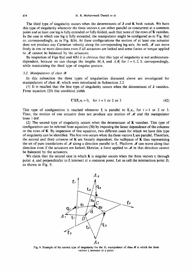
We claim that the second case in which K is singular occurs when the three vectors ti through point A~ and perpendicular to f~ intersect at a common point. Let us call the intersection point D, as shown in Fig. 9.

f'T A 3

s / , q3

Az

f3

Fig. 9. Example of the second type of singularity for the 3L manipulator of class ~t in which the three vectors t~ intersect at a point.


Since the three vectors f~, for i = 1, 2, 3, are coplanar, we can write f3 in terms of the first two, namely,

f3 = 0q fl + e2f2 (43)

Moreover, the inner product of boths sides of equation (43) by vector d, leads to

frd = ~, fTd + ~2f~d (44)

where d is the vector directed from C and D. But we have

f,Tti = 0, for i = 1,2,3

Then, equation (44) can be written as

f]'(d + t3) = e~ fT(d + t~) + e2 f~(d + t:) (45)

Moreover, we have

d + ti = - (qi + si), for i = 1, 2, 3

Substituting the values of d + t~, for i = 1, 2, 3, from the foregoing equation into equation (45), yields

fT(q3 + S3) = el flT(ql + Sl ) + a2 fT(q2 + S2) (46)

Moreover, from equation (43) it is apparent that

fTE = a, fTE + a2f~E (47)

From equations (46) and (47), it is obvious that we can write the third row of K as a linear combination of the first two rows, the claim thus being made apparent.

Then, the nullspace of K represents the set of pure rotations of J / a b o u t the common intersection point D. The platform ~ ' can thus rotate about that point even if the actuators are locked; likewise, a moment applied to J / c a n n o t be balanced by the actuators.

(3) The third type of singularity occurs when the determinants of J and K both vanish. Then, we have this type of singularity whenever the two types of singularities converge.

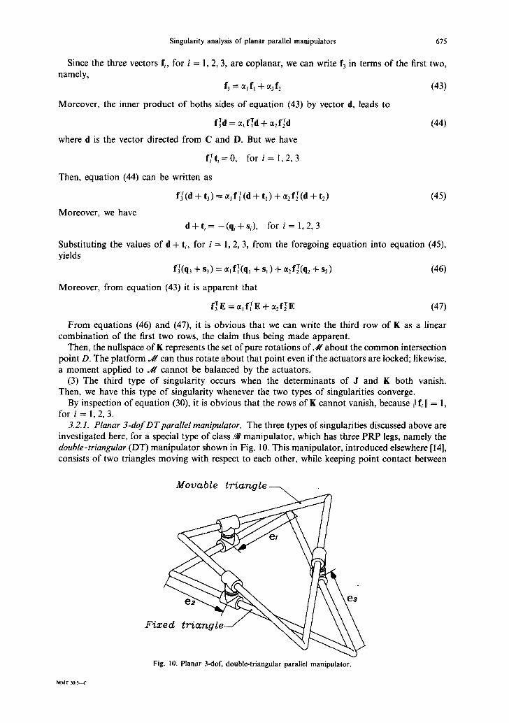
By inspection of equation (30), it is obvious that the rows of K cannot vanish, because JI f~ II = l, for i = l, 2, 3. 3.2.1. Planar 3-dofDTparallel manipulator. The three types of singularities discussed above are investigated here, for a special type of class N manipulator, which has three PRP legs, namely the double-triangular (DT) manipulator shown in Fig. 10. This manipulator, introduced elsewhere [14], consists of two triangles moving with respect to each other, while keeping point contact between

M o v a b l ~ .

Fixed triang ,~

Fig. 10. Planar 3-dof, double-triangular parallel manipulator.

MMT 30/5--C

676 H. R. Mohammadi Daniali et al.

.M (Movable)

~ 2

e a ~ ~ (Fixed)

R, f' Fig. l 1. Example of the first type of singularity for the DT manipulator.

every pair of edges. Moreover, the movable triangle is moved by actuating three prismatic joints along the sides of the fixed triangle, namely {ei}~.

It is recalled that the first type of singularity occurs when the determinant of d vanishes. Upon assigning E~ = (1/lleill)l, equation (42) leads to

1 Ile, llf~Eei=0' f o r i = l or2or 3 (48)

f 2

e ~ ~ B (Fixed)

% Fig. 12, Example of the second type of singularity for the DT manipulator.

.M

Singularity analysis of planar parallel manipulators

e ~ B (Fixed) f \ A

(Movable) ~ ~ ~

-<. Fig. 13. Example of the third type of singularity for the DT manipulator.

677

This type of configuration is reached whenever ei and fi, for i = 1 or 2 or 3, coincide, which means that one or more edges of the triangles coincide, as shown in Fig. 11. At this configuration the motion of the ith actuator does not produce any motion of moving triangle J- /and the manipulator cannot move along a direction perpendicular to the coincident edges.

The second type of singularity occurs when the determinant of K vanishes. As we explained in Subsection 3.2, this type of singularity arises in two cases. The first occurs when the three vectors fi are parallel, but such a manipulator is not a DT manipulator and is thus left aside. The second case in which K is singular occurs when the three vectors t~, perpendicular to f~, intersect at a common point D, as shown in Fig. 12. At this configuration the moving triangle J / / can undergo a finite rotation about D, even if the actuators are locked; likewise, a torque applied to ~ ' cannot be balanced by the actuators.

The third type of singularity occurs when the determinants of J and K both vanish. We have this type of singularity whenever the three perpendiculars to the three edges of the moving triangle intersect at a common point and at least one pair of the edges of the two triangles coincide, as shown in Fig. 13. At this configuration the motion of one actuator does not produce any Cartesian velocity and the manipulator loses I dof. As well, the moving triangle ~/ can undergo a finite rotation about D, even if the actuators are locked; likewise, a torque applied to ~ ' cannot be balanced by the actuators.

Again, for DT manipulators this type of singularity is not architecture-dependent, since we can find one point in the moving triangle d¢ from which we can draw three perpendiculars to the three edges. Let us call the intersection points R~, for i = I, 2, 3, as shown in Fig. 13. It is obvious that any three lines passing through points R~ such that one of them coincides with one of the edges of the moving triangles can form the fixed triangle 8 . Needless to say, such a triangle is not unique. In other words, we can choose the fixed and moving triangles arbitrarily.

4. CONCLUSIONS

The Jacobian matrices of two classes of planar parallel manipulators were derived. The first class consists of 20 different manipulators constructed with three, three-degree-of-freedom legs,


namely PRR, PPR, R R R and RPR, in which P and R represent prismatic and revolute pairs, respectively. The second class consists of 4 different manipu la to rs constructed with three, three- degree-of-freedom legs, namely PRP and RRP. A general classification of para l le l -manipula tor singularities into three groups was described and identified for the two classes of manipula tors . Finally, one example for each class was concluded. Cont ra ry to earlier claims, we have shown that the third type of singulari ty is not necessarily architecture-dependent .

Acknowledgements--This research work was supported by NSERC (Natural Sciences and Engineering Research Council, of Canada) under Grants A4532, A4219, STRGP 205, and EQP00-92729. Support from IRIS, the Institute for Robotics and Intelligent Systems, a network of Canadian centres of excellence, is also acknowledged. The first author was funded by the Ministry of Culture and Higher Education of the Islamic Republic of Iran.

R E F E R E N C E S 1. K. Sugimoto, J. Duffy and K. H. Hunt, Mech. Mach. Theory 17(2), 119-132 (1982). 2. F. L. Litvin and V. Parenti-Castelli, ASME J. Mech. Transmissions Automatn Design 107, 170-178 (1985). 3. F. L. Litvin, V. Parenti-Castelli and C. Innocenti, Int. J. Robotics Res. 5(2), 52-65 (1986). 4. K. H. Hunt, Robotica 4, 171-179 (1986). 5. K. H. Hunt, Robotica 5, 17--22 (1987). 6. Z. C. Lai and D. C. H. Yang, Int. J. Robotics Res. 5(2), 66-74 0986). 7. J. Angeles, K. Anderson, X. Cyril and B. Chen, ASME J. Mech. Transmissions Automatn Design 110, 246-254 0988). 8. T. Shamir, Int. J. Robotics Res. 9(1), 113-121 (1990). 9. J.-P. Merlet, Int. J. Robotics Res. 8(5), 45-56 (1989).

10. C. Gosselin and J. Angeles, IEEE Trans. Robotics Automatn 6(3), 281-290 (1990). ll. O. Ma and J. Angeles, Int. J. Robotics Automatn 7(1), 23-29 (1992). 12. C. M. Gosselin and J. Sefrioui, Proc. of the ASME Mechanisms Conf., 329-335, Phoenix, (1992). 13. H. R. Mohammadi Daniali, P. J. Zsombor-Murray and J. Angeles, Proc. of ASME Conf. on Design Automation,

593-599, New Mexico (1993). 14. H. R. Mohammadi Daniali, P. J. Zsombor-Murray and J. Angeles, Computational Kinematics (J. Angeles, G. Hommel

and P. Kovfics, eds.), pp. 153-164. Kluwer, Dordrecht (1993).

ANALYSE DES SINGULARITIES DES M A N I P U L A T E U R S P A R A L L [ L E S P L A N S

R6smn#--Cet article pr6sente une classification g~n6rale des singularit~s relatives aux manipulateurs parall61es de type plan, bas6e sur les propri6t~s de leurs matrices jacobiennes. Les auteurs ~tudient notamment les matrices jacobiennes de deux cat6gories de manipulateurs parall61es et classent leurs singularit~s dans trois types. La premiere cat~gorie regroupe vingt manipulateurs construits avec trois diff6rentes combinaisons de pattes de types PRR, PPR, RRR et RPR, off Pest un couple prismatique et R, un couple rotoi'de. La deuxi6me cat6gorie rassemble quatre manipulateurs construits avec trois pattes de types PRP et RRP. Enfin, les auteurs donnent des exemples des trois types de singularit~ dans chaque cat6gorie, Contrairement dce qui a 6t6 affirm~ pr6c6demment, les auteurs d6montrent que les singularit6s appartenant au troisi~me type ne d~pendent pas n6cessairement de I'architecture du manipulateur, mais peuvent se retrouver dans des manipulateurs d'architecture arbitraire.

Singularity analysis of planar parallel manipulators

Documents

Transcript of Singularity analysis of planar parallel manipulators