University of Louisville University of Louisville

ThinkIR: The University of Louisville's Institutional Repository ThinkIR: The University of Louisville's Institutional Repository

Electronic Theses and Dissertations

12-2021

Additive manufacturing using robotic manipulators, FDM, and Additive manufacturing using robotic manipulators, FDM, and

aerosol jet printers. aerosol jet printers.

Alexander Curry University of Louisville

Follow this and additional works at: https://ir.library.louisville.edu/etd

Part of the Electrical and Electronics Commons, Electronic Devices and Semiconductor Manufacturing

Commons, Manufacturing Commons, and the Nanotechnology Fabrication Commons

Recommended Citation Recommended Citation Curry, Alexander, "Additive manufacturing using robotic manipulators, FDM, and aerosol jet printers." (2021). Electronic Theses and Dissertations. Paper 3797. Retrieved from https://ir.library.louisville.edu/etd/3797

This Master's Thesis is brought to you for free and open access by ThinkIR: The University of Louisville's Institutional Repository. It has been accepted for inclusion in Electronic Theses and Dissertations by an authorized administrator of ThinkIR: The University of Louisville's Institutional Repository. This title appears here courtesy of the author, who has retained all other copyrights. For more information, please contact thinkir@louisville.edu.

ADDITIVE MANUFACTURING USING ROBOTIC MANIPULATORS, FDM, AND

AEROSOL JET PRINTERS

By

Alex Curry

B.S.E., Murray State University, 2019

A Thesis

Submitted to the Faculty of the

J. B. Speed School of Engineering of the University of Louisville

in Partial Fulfillment of the Requirements

for the Degree of

Master of Science in Electrical Engineering

Department of Electrical & Computer Engineering

University of Louisville

Louisville, Kentucky

December 2021

Copyright 2021 by Alex Curry

All rights reserved

ii

ADDITIVE MANUFACTURING USING ROBOTIC MANIPULATORS, FDM, AND

AEROSOL JET PRINTERS

By

Alexander Thomas Curry

B.S.E., Murray State University, 2019

A Thesis Approved on

November 23, 2021

By the following Thesis Committee:

__________________

Dr. Dan Popa

__________________

Dr. Kevin Walsh

__________________

Dr. John Naber

__________________

Dr. Thad Druffel

iii

DEDICATION

I would like to dedicate this thesis to my mom and dad, whose unwavering

support has given me the freedom to pursue my passions and continually progress as an

individual. I would like to also dedicate this thesis to my committee, many of whom

played a large role in my decision to attend the University of Louisville, my friends that

are constantly pushing me and always there to lend a hand, and my colleagues, who I

have learned far more from than I could have ever imagined.

iv

ACKNOWLEDGMENTS

I would like to thank Dr. Dan Popa for guiding me and giving me the opportunity

to be a part of LARRI, for which I will be forever grateful. I would also like to thank Dr.

Kevin Walsh for introducing me to research at UofL and always giving me great advice

for research and life. I am also grateful to Dr. John Naber for all the learning

opportunities in class and independent projects, as well as Dr. Thad Druffel for all his

help pointing us in the right direction with IPL and NovaCentrix ink. I am also thankful

to all the staff of LARRI, especially Mrs. Johanna Boone and Mrs. Laurie Ann Huelsman

for constantly keeping the research team organized, facilitating meetings, and managing

us so that we could focus on research. Furthermore, I would like to thank the team of

researchers I worked closest with: Andriy Sherehiy, Dilan Ratnayake, Alireza Tofangchi,

Moath Alqatamin, Danming Wei, Scott Nimon, Ola Olowo, Ruoshi Zhang, and Doug

Jackson. Every single one of them welcomed me with open arms when I joined the

research team and each of them have taught me a tremendous amount along the way.

Finally, I want to thank Louisville’s Automation and Robotics Research Institute

(LARRI), the National Nanotechnology Coordinated Infrastructure (NNCI), and the

National Science Foundation (NSF) Awards ECCS-2025075 and ECCS-1828355 for

supporting this research.

v

ABSTRACT

ADDITIVE MANUFACTURING USING ROBOTIC MANIPULATORS, FDM, AND

AEROSOL JET PRINTERS

Alexander Thomas Curry

December 3, 2021

Additive manufacturing has created countless new opportunities for fabrication of

devices in the past few years. Advances in additive manufacturing continue to change the

way that many devices are fabricated by simplifying processes and often lowering cost.

Fused deposition modeling (FDM) is the most common form of 3D printing. It is a well-

developed process that can print various plastic materials into three-dimensional

structures. This technology is used in a lot of industries for rapid prototyping and

sometimes small batch manufacturing. It is very inexpensive, and a prototype can be

created in a few hours, rather than days. This is useful for testing dimensions of designs

without wasting time and money. Recently, a new form of additive manufacturing was

developed known as aerosol jet printing (AJP). This process uses a specially developed

ink with a low viscosity to print a wide range of metals and polymers. These printers

work by atomizing the ink into a mist that is pushed out of a nozzle into a focused beam.

This beam deposits material on the substrate at a standoff distance of 3-5 mm. Since this

is a non-contact printing process, many non-planar surfaces can be printed on quite

easily. AJP also offers very small feature sizes as low as 30 µm. It is useful for printing

conductive traces and printing on unique surfaces. These printed traces often need some

form of post processing to fully cure the ink and remove any solvent. For metals such as

vi

silver, this post processing removes solvent, increases conductivity, and increases

adhesion. Methods for post processing include using an oven, intense pulse light (IPL), or

a laser that follows the traces as they are printed. Of these methods, the IPL offers the

greatest flexibility because it can cure a larger area than the laser and only takes a few

seconds compared to hours in an oven. In this thesis, these two types of additive

manufacturing processes, FDM and AJP, are explored, developed, and integrated with

robotic manipulators in a custom system called the “Nexus”. By integrating these

processes with robotic manipulators, these processes can be automated and combined to

create unique processes and streamlined fabrication. The third chapter covers the

development of the AJP printing and curing processes and integration with the Nexus

system as well as some example devices such as a strain gauge. The fourth chapter goes

over how a custom FDM module was integrated into the Nexus system and how material

extrusion is synchronized with the motion component. Finally, in the second part of the

fourth chapter, an FDM 3D printer is designed and fabricated as an end effector for a

6DOF robotic arm to be used in the Nexus system. To control these processes, G-Code is

used to tell the machines the correct path to take. Methods for generating 5-axis G-Code

are suggested to enable non-planar printing in the future.

vii

TABLE OF CONTENTS

DEDICATION ................................................................................................................... iii

ACKNOWLEDGMENTS ................................................................................................. iv

ABSTRACT ........................................................................................................................ v

CHAPTER I ........................................................................................................................ 1

1.1 Motivation ................................................................................................................. 1

1.2 Challenges ................................................................................................................. 2

1.3 Contributions ............................................................................................................. 3

1.4 Thesis Organization ................................................................................................... 5

CHAPTER II ....................................................................................................................... 7

2.1 FDM 3D Printing ...................................................................................................... 7

2.2 Aerosol Jet Printing ................................................................................................... 8

2.3 Strain Gauges .......................................................................................................... 10

2.4 Intense Pulse Light .................................................................................................. 11

2.5 Nexus System .......................................................................................................... 12

CHAPTER III ................................................................................................................... 14

3.1 Characterizing the conductivity of aerosol jet printed silver features on glass ....... 14

3.2 Clariant Ag Printing Recipe .................................................................................... 14

3.3 Oven Sintering Process ........................................................................................... 16

3.4 Conductivity Measurement using Van Der Pauw Method ...................................... 16

3.5 Predicting Conductivity in the Oven Using a Linear Regression Equation ............ 19

viii

3.6 NovaCentrix Ag Printing Recipe ............................................................................ 22

3.7 Strain Gauge Sintering and Characterization .......................................................... 23

3.8 Results and Discussion ............................................................................................ 24

3.9 Curing printed silver traces using intense pulse light.............................................. 28

3.10 Nexus AJP Manufacturing Sequence .................................................................... 32

3.11 Summary ............................................................................................................... 34

CHAPTER IV ................................................................................................................... 35

4.1 Stationary FDM 3D Printer Module ........................................................................ 35

4.2 Component Selection .............................................................................................. 35

4.3 Design of Custom Extruder Mount and Control Box ............................................. 36

4.4 Control and Synchronization ................................................................................... 38

4.5 Printing Process ....................................................................................................... 40

4.6 Printing Results ....................................................................................................... 41

4.7 FDM End Effector for a Robotic Manipulator ........................................................ 44

4.8 FDM End Effector Design Philosophy ................................................................... 45

4.9 Mechanical Design .................................................................................................. 46

4.10 Electrical Design ................................................................................................... 47

4.11 Fabrication ............................................................................................................. 49

4.12 Software ................................................................................................................ 50

4.13 Installation ............................................................................................................. 53

4.14 Results ................................................................................................................... 55

4.15 Creating 5-Axis G-Code for 6DOF Robotic Tools ............................................... 58

4.16 Summary ............................................................................................................... 61

ix

CHAPTER V .................................................................................................................... 63

REFERENCES ................................................................................................................. 65

APPENDIX A ................................................................................................................... 68

APPENDIX B ................................................................................................................... 71

APPENDIX C ................................................................................................................... 76

CURRICULUM VITAE ................................................................................................... 79

x

LIST OF TABLES

Table 3.1 Conductivity Results from Curing in the Oven................................................ 18

Table 3.2 AJP Printing Recipe for 50 µm Traces Using NovaCentrix Ag ink ................ 22

Table 3.3 Experimental and Theoretical Strain Data ....................................................... 26

Table 3.4 Experimental Data for Printed Strain Gauge ................................................... 27

Table 3.5 IPL Recipe for AJP NovaCentrix Ag Ink ........................................................ 29

Table 3.6 Thickness Data of Strain Gauge Turns Measured Optically ............................ 31

Table 4.1 Pinout of FDM End Effector Connections from ATI ToolChanger ................ 48

xi

LIST OF FIGURES

Figure 2.1 Diagram of a Typical FDM 3D Printer ............................................................ 8

Figure 2.2 Schematic of the Aerosol Jet Printing Process ............................................... 10

Figure 2.3 Nexus System Major Components: (1) 6-DOF positioner, (2) Optomec AJP,

(3) Stationary FDM 3D Printer, (4) PicoPulse Inkjet Printer, (5) IPL, (6) Microscope

Inspection Station.............................................................................................................. 13

Figure 3.2 Van der Pauw Conductivity Measurement Using Four Point Probe Station .. 17

Figure 3.3 Output Data From Linear Regression Algorithm ........................................... 20

Figure 3.4 Residual Analysis to Check for Model Adequacy .......................................... 21

Figure 3.5 (a) Strain Gauge Design, (b) Printed Strain Gauge with Dimensions ............ 23

Figure 3.6 Schematic of the Cantilever Beam with a Strain Gauge ................................ 24

Figure 3.7 (a) Mounted Printed and Reference Strain Gauge on Metal Beam (b) and

Strain Gauge Measuring Setup Using Micrometer ........................................................... 25

Figure 3.8 (∆R/R) vs Strain for Printed Strain Gauge ..................................................... 28

Figure 3.9 Power vs Time of IPL Recipe Step 1 (left) and Step 2 (right) ....................... 29

Figure 3.10 (Left) 700 Ω gauge that was cured successfully using the recipe from Table

3.5 (Right) Gauge with unsuccessful curing – material at the turns is much thicker. ...... 31

Figure 3.11 AJP Printed 4x4 Sensor Array on Kapton .................................................... 33

Figure 4.1 Stationary FDM Module Extruders Mounted in Nexus System..................... 37

Figure 4.2 FDM Module Control Box ............................................................................. 38

Figure 4.3 G-Code Example with Resulting Toolpath Highlighted ................................ 39

xii

Figure 4.4 Flowchart of 3D Printing Process for Nexus System ..................................... 41

Figure 4.5 First Test Print Accidently Mirrored Across Y-Axis ..................................... 42

Figure 4.6 (Left) “UofL” Test Print (Right) CAM vs Positioner Axes Orientation ........ 42

Figure 4.7 3D Print of a 15 mm Tall Cylinder with a Diameter of 25 mm Using PLA .. 43

Figure 4.8 Bowden vs Direct-Drive Extruder [31] .......................................................... 45

Figure 4.9 CAD Design of FDM End Effector ................................................................ 47

Figure 4.10 Mostly Assembled FDM End Effector Prototype ........................................ 50

Figure 4.11 FDM End Effector Positioned on Tool Changer Rack ................................. 54

Figure 4.12 FDM End Effector Picked Up by Denso Robotic Arm ................................ 55

Figure 4.13 FDM End Effector Testing Setup Using Robotic Manipulator .................... 57

Figure 4.14 Measuring Dimensions of Sample Print Using Digital Calipers .................. 57

Figure 4.15 FDM End Effector Printing at a 45° Angle .................................................. 58

Figure 4.16 (Left) Stair-stepping effect from Traditional Printing, (Right) Non-planar

Print [32] ........................................................................................................................... 59

1

CHAPTER I

INTRODUCTION

1.1 Motivation

The main motivation of this work is to contribute to and facilitate advances in

additive manufacturing. Additive manufacturing has been around for a while now, but

some technologies such as Fused Deposition Modeling (FDM) are waiting for the next

big breakthrough. Although the process behind FDM is well explored, the toolpaths to

form three-dimensional objects still have plenty of room for improvement. Future slicing

software for 3D printers will probably be able to print non-planar layers, but in order to

print non-planar layers efficiently, the nozzle of the FDM printer must be able to change

its angle relative to the surface being printed on in order to avoid collisions. This is a

major motivation behind the development of the two FDM modules presented in this

thesis and some thought is also given to how these non-planar toolpaths might be

generated for initial testing of non-planar printing.

As an emerging technology in additive manufacturing and printed electronics,

aerosol jet printing (AJP) is still very new and there are nowhere near as many published

papers on the topic when compared to FDM. Therefore, another motivation of this thesis

is to develop printing recipes for AJP and explore optimal curing methods. Since this

printing process utilizes an ink to print, the curing step after printing is extremely

2

important and cannot be overlooked. Two curing methods, an oven and intense pulse

light (IPL), are mentioned in this thesis and successful recipes are developed using both

methods. However, the IPL has one main advantage over the oven – rapid curing.

Therefore, another motivation is to develop recipes using the IPL that are competitive

with results gained previously using an oven.

1.2 Challenges

The previous section discussed the big picture motivation behind the technologies in

this work, but this section will go through specific challenges associated with those

motivations. The first challenge is integration of all these technologies into the Nexus

system. The Nexus system is explained in detail in chapter 2.5. Every technology in this

thesis began outside of the Nexus system with the intention of integration eventually

taking place. This is a challenge because the Nexus is a custom tool developed at the

University of Louisville and therefore the solutions to integrate each technology into the

system must also be customized.

For the FDM stationary module, the main challenge is synchronization of the

extrusion with the motion of a 6 degree of freedom (DOF) positioner. Normally, a single

controller synchronizes x-y-z motion of the printer with the extrusion of material, but in

this case two separate controllers must be synchronized. The solution to this challenge is

discussed in chapter 4.4.

As for the AJP, several challenges must be solved including developing reliable

printing recipes, successful integration into the Nexus and finding reliable curing recipes.

The manufacturers of AJP inks often give an initial recipe to try, but this recipe must be

tuned to the user’s requirements. The recipe provided began with a trace width of 100

3

µm, but since smaller feature sizes were desired, this recipe was changed until consistent

50 µm lines were developed. Then recipes also must be developed to cure these traces

after printing. Curing using an oven is fairly straightforward, having only two parameters,

time and temperature. However, the IPL has many more parameters to change and the

physics behind the curing is different than the oven. This makes finding a consistent

recipe for the IPL much more difficult.

Finally, the FDM end effector involved many challenges mainly due to the design

constraints. The tool needed to be self-contained with every component of the FDM

system located on the tool itself. This is very challenging due to weight and space

constraints. Also, all signals and power to the tool must be realized using a maximum of

15 wires, since the tool changer the Nexus system uses only has 15 connections.

Furthermore, custom software had to be developed in LabVIEW to control and

synchronize the tool with the motion of a 6-DOF robotic arm. Adding all the constraints

together makes for a very challenging design.

1.3 Contributions

In this thesis, we describe two major contributions to the Nexus multiscale

manufacturing system including 1) The development and integration of custom FDM

systems in the Nexus system, and 2) Process development for manufacturing of tactile

skin sensors on flexible substrates using the AJP, IPL and 6-DOF positioner on the

Nexus.

For the stationary FDM module, custom mounting solutions were designed and

fabricated and the FDM system was installed and wired to a custom electrical control

box. Then, software was developed to ease integration with the Smoothieboard, a 3D

4

printer control board to be used in tandem with the Newport motion controller. This

software was utilized in the main LabVIEW user interface (UI) and synchronization of

the two controllers using G-Code sent simultaneously was proposed.

For the FDM end effector, initial design ideas were discussed with colleagues and

then a preliminary design was completed in CAD. This CAD design was discussed with

colleagues once again and constructive criticism was received to refine the design.

Iterations of this process continued, until the final version of the CAD design (v64) was

completed for the final design of the prototype. The prototype was fabricated as part of

this research and custom software in LabVIEW was developed from scratch to control

the tool. A journal paper is currently being worked on to share the results of this design

and its unique self-containment of all FDM components.

Finally, contributions were made to help facilitate development of printing recipes

for the AJP for two silver inks from Clariant and NovaCentrix. A reliable recipe for 50

µm wide traces was developed with colleagues and major contributions were made to

help realize the generation of printing toolpaths using Fusion 360 to generate G-Code for

the system. A guide to generating G-Code using Fusion 360 can be found in Appendix B.

As an outcome of my research, two conference papers were also published to the

2021 MSEC conference and the 2021 IEEE FLEPS conference. The MSEC paper

develops a model for curing AJP silver traces using an oven and the IEEE FLEPS paper

explores a custom application of AJP by printing a strain gauge on flexible Kapton.

Another journal paper is also being written that will share new curing recipes using the

IPL and more evaluation of printed strain sensors.

5

1.4 Thesis Organization

Chapter 1 begins by covering the motivation behind the research. It goes through

the challenges associated with the different technologies presented and provides some

background on the current state of these technologies. The chapter also covers the

contributions made to the included technologies thus far and papers that have been

published as well as future papers that are being planned. Finally, the chapter ends by

giving an overview how this thesis is organized.

Chapter 2 provides background on several technologies discussed throughout this

thesis. The first technology is fused deposition modeling (FDM). The second technology

is aerosol jet printing (AJP). After AJP, intense pulse light (IPL) is covered since some

form of curing normally follows AJP. Then, the Nexus system is introduced, and some

basic specifications are supplied to give the reader a basic understanding of the system.

Chapter 3 covers the processes developed for the AJP system. A design of

experiment (DOE) is discussed that was developed to characterize the printing and curing

of Clariant silver ink using an oven. Afterwards, another recipe is developed for a new

silver ink from NovaCentrix and a strain gauge is printed and evaluated to compare its

competitiveness to commercial metal-foil strain gauges. Finally, curing using the IPL

instead of the oven is introduced and initial results and a working recipe are shared.

Chapter 4 goes into more detail about the stationary FDM module integrated into

the Nexus system. It begins by covering the components selected and some of the custom

design solutions for the system. Then the realization for control of the printer and

synchronization with the Newport 6-DOF positioner is discussed. This leads into a

flowchart of the printing process from CAD to finished 3D printed part specifically for

6

the Nexus system. Printing results are then shared and the chapter ends with a summary

of the information presented.

The second part of chapter 4 discusses the FDM end effector designed to be

attached to a robotic manipulator. It begins by discussing the ideas behind the design and

constraints that were considered while designing the tool as well as components selected.

Then it covers the main two aspects of the design – the mechanical design of the tool and

then the electrical design of the tool. Afterwards, a prototype is fabricated and software is

developed to control the tool through LabVIEW. Basic functionality of the prototype and

software is tested and a simple test print is performed using G-Code. The chapter

concludes by discussing possible methods of generating 5-axis G-Code that can be used

to achieve non-planar printing with both FDM tools that are integrated into the Nexus

system.

Chapter 5 provides a conclusion to the thesis.

7

CHAPTER II

BACKGROUND

2.1 FDM 3D Printing

One of the most common forms of additive manufacturing and specifically 3D

printing is fused deposition modeling. FDM printing works by taking a polymer and

melting it in order to extrude it into a 3D structure. The technology required to

accomplish this is fairly straightforward. Polymers such as Polylactic Acid (PLA),

PolyCarbonate, Acrylonitrile butadiene styrene (ABS), etc. are processed into very long

strands of 1.75 mm diameter or 3 mm diameter and wound around a roll. This is how

filament is created. This filament is then fed into an extruder, which uses internal gears to

grip the filament and pull it down into the heatblock. The gears inside an extruder are

usually driven by a stepper motor for precise control. The heatblock is heated to some

temperature above the glass transition temperature of the filament. As the filament

reaches the heatblock, it is melted into a molten plastic [1]. A diagram of this process can

be seen in Figure 2.1. As more filament is pushed in, the molten plastic is forced out of a

smaller diameter nozzle, usually 0.4 mm or 0.6 mm. As the molten plastic is extruded, the

motion system of the 3D printer follows a pre-defined toolpath to distribute the molten

plastic one layer at a time. Each layer is built on top of the previous one and the molten

plastic cools and hardens shortly after being deposited. This process continues in order to

8

build a 3D structure. Some prints can take hours or even days depending on the size of

the 3D model.

Figure 2.1 Diagram of a Typical FDM 3D Printer

2.2 Aerosol Jet Printing

The concept of aerosol jet printing (AJP) was developed by a Mesoscale

Integrated Conformal Electronics (MICE) project that was funded by the Defense

Advanced Research Projects Agency (DARPA) in the 1990s [2]. The goal of this funded

project was to develop a process capable of conformally depositing a wide range of

materials on nearly any substrate. AJP is now commercialized by Optomec, Inc., who

holds several patents for their AJP process [3]. A typical AJP system consists of two

9

major components (atomizing the raw materials and depositing focused material), as

shown in Figure 2.2. AJP works by placing ink into either an ultrasonic or pneumatic

atomizer that turns the liquid ink into a dense mist. The mist is routed to the deposition

head where it becomes focused by a controlled sheath gas, usually Nitrogen. As the

aerosol stream and gas pass through the nozzle, they form a tight beam and accelerate.

This high velocity stream remains in tight formation from the nozzle all the way to the

substrate, which is typically 2-5 mm away from the nozzle [4]. The AJP process can print

features as small as 10 microns all the way up to over a millimeter [5, 6]. This is achieved

by utilizing different nozzle sizes.

AJP has an extremely wide range of printable materials. Metals such as gold,

platinum, silver, and copper can be made into inks as well as polymers such as polyimide,

PEDOT, and SU-8 just to name a few [7]. AJP can also print semiconductor materials,

resistors, dielectrics/insulators, carbon, resists, and even carbon nanotubes. Any

substance that can be manufactured into some form of ink is most likely compatible with

the AJP process. Typically, any ink that has a viscosity between 1-1000 cP is printable,

although this range of values changes depending on the type of atomization used. The

quality and composition of the ink is very important to the final morphology and

characteristics of the material after printing. Most materials also require some form of

post processing to finalize their properties. Post processing is usually done by sintering

the material in the oven [8], curing with intense pulse light [9], or sintering with a laser

over the same contours printed. Some materials can also be cured by UV light, although

most printable metals do not fall into this category.

10

Figure 2.2 Schematic of the Aerosol Jet Printing Process

2.3 Strain Gauges

As one of the applications for AJP, a strain gauge is a device whose electrical

resistance changes in proportion to the amount of strain placed on the device [10]. Strain

gauges can be designed using the following equation:

R = ρ*(L/A) (2.1)

Where R is the overall resistance of the strain gauge, L is the composite length of the

meandering trace, A is the cross-sectional area of an individual trace, and ρ is the average

11

resistivity of the material. This equation will be used to design a printable strain gauge in

section 3.6.

As one of the most common form factors of a strain gauge, a metal foil strain

gauge consists of thin wire or foil structured in a back-and-forth serpentine design. These

are often used as sensors in systems to measure forces, moments, and the deformations of

structures and materials. When the metal trace of a strain gauge is stretched with a

parallel force, a dimensional change occurs in the trace, which causes L to increase, A to

decrease, and its overall resistance to consequently increases, according to equation (2.1).

This assumes the material’s resistivity is independent of the strain, as is the case with

most metals. The primary figure of merit of a strain gauge is its “gauge factor” or GF,

which is a measure of how sensitive the device is to a given applied strain. The equation

for GF is provided below [11]:

GF = (∆R/R) / ɛ (2.2)

Where GF is the gauge factor, ε is the applied strain, R is the device’s nominal

resistance under no loading conditions, and ΔR is the measured change in resistance to

the applied strain. As described in equation (2.2), if we know the strain and the

corresponding change in resistance, the GF can be calculated. This will be further

explored later on in section 3.7, with a strain gauge printed using Ag ink with an AJP.

2.4 Intense Pulse Light

IPL is an ideal sintering strategy for metal nanoparticle inks because it promotes

rapid large area curing and can be used with substrates that cannot withstand thermal

curing in the oven. IPL works by using a xenon lamp that emits a wide range of

12

wavelengths from ultraviolet to infrared with the highest intensity wavelengths in the

visible light range. Using a pulse with a duration shorter than the time it takes to reach the

thermal equilibrium of a nanoparticle ink allows the ink to sinter without transferring

very much energy to the substrate [12]. There are three steps that happen during the

sintering of metal nanoparticle inks: evaporation of the solvent, removal of dispersants

and binder materials by thermal decomposition, and neck formation and grain growth

[13]. One major shortcoming of IPL is that it is a top-down sintering method. This means

that thicker traces require more energy to cure all the way through, making it difficult and

sometimes impossible to sinter all the way through. Despite this downfall, IPL is a very

attractive method for post-processing printed metal nanoparticle inks so long as they are

deposited with a uniform thickness and kept fairly thin (< 5 µm). IPL has also been

shown to offer over twice the conductivity than thermal sintering in the oven according to

a study that compared different sintering methods [14].

2.5 Nexus System

The Nexus system is a multi-scale additive manufacturing system that

incorporates several subsystems to combine processes and realize automated assembly of

micro-scale devices [15]. At the time of this writing the Nexus system includes a 6-DOF

Denso robotic arm suspended from an X-Y gantry, a 4-DOF Denso SCARA robot, a

stationary FDM 3D printer, an Optomec Aerosol Jet Printer, a Picopulse Inkjet Printer, a

Xenon Intense Pulse Light Unit, an inspection station, and a 6-DOF positioner that can

move from one station to the next to facilitate novel processes. All of these subsystems

are contained in an extruded aluminum frame measuring 3960 mm x 3530 mm x 2215

mm (L x W x H) [16]. The Nexus system was designed to realize automated assembly of

13

micro-scale devices and facilitate rapid prototyping. Typically, devices such as Micro

Electromechanical Devices (MEMS) are fabricated one step at a time and assembly is

performed manually in a cleanroom. An engineer must perform one process then take the

device to the next machine to perform the next step. This procedure is repeated for the

entire fabrication process until a device is completed. The Nexus system combines many

manufacturing tools into one so that these fabrication processes can be automated. This

also creates the opportunity to invent new novel processes that might not otherwise be

possible using manual assembly. This thesis will focus on the two FDM modules, the

AJP, and IPL.

Figure 2.3 Nexus System Major Components: (1) 6-DOF positioner, (2) Optomec AJP,

(3) Stationary FDM 3D Printer, (4) PicoPulse Inkjet Printer, (5) IPL, (6) Microscope

Inspection Station

2

1

3 4 5 6

14

CHAPTER III

PRECISION SENSOR MANUFACTURING USING THE NEXUS

3.1 Characterizing the conductivity of aerosol jet printed silver features on glass

Section 3.1 through 3.5 contains material that has been published as a conference

paper [17]. The study from this paper used an Aerosol Jet Print Engine with a Decathlon

Print Cassette from Optomec for all printing processes. An ultrasonic atomizer was used

to atomize a silver ink made by Clariant. After printing, the silver ink was cured in an

oven in ambient conditions. The focus of this study was to characterize the response of

the Clariant silver ink in the oven with varying time and temperature and measure the

resulting conductivity. Using these results, a statistical model was developed to show

how the conductivity changed with time and temperature using a linear regression model.

This resulted in an equation that can be used for oven curing to predict the conductivity

of the printed silver traces within the range observed in the study.

3.2 Clariant Ag Printing Recipe

For this experiment, the Optomec Decathlon engine was set to have a flow rate of

25 sccm, a sheath value of 30 sccm, and a divert and boost value of 50 sccm. The

transducer was set to 500 mA and the Ultrasonic Atomizer bath was set to a temperature

of 23 - close to room temperature. These parameters were set using the KEWA

process control software, provided by Optomec. The other parameters used that were set

outside the KEWA software include setting the chiller to 15 and diluting the Clariant

15

silver ink with deionized (DI) water. A ratio of 3:1 DI water to ink was used to lower the

viscosity of the ink to the acceptable range – between 1-10 cP for the ultrasonic

Decathlon print engine. These settings gave an average line width of 150 μm when

examined under the microscope. The line width was always verified under the

microscope before printing samples for the experiment to ensure consistency. All printing

processes done in this study used these parameters and were printed at a speed of 5 mm/s.

Once the print engine was tuned, 3x3 mm Van der Pauw square pads were printed on a 2-

inch glass slide using a shadow mask as shown in Figure 3.1. A shadow mask was used

for this part of the research to improve the perimeter edge quality of the silver pads. A

slightly overlapping serpentine structure was programmed to print the pads by adjusting

the steps in the x-direction of the toolpath to prevent any gaps. After printing, the Van der

Pauw silver pads were sintered in the oven at a wide variety of times and temperatures.

Figure 3.1 Printed Silver Pads Using the Shadow Mask

16

3.3 Oven Sintering Process

Thermal curing using an oven is one of the most reliable curing approaches for

nanoparticle inks. Initial heating of the printed features leads to the evaporation of the

solvent, making the nanoparticles come in contact with each other. Further heating leads

to fusion and causes the material to form a continuous layer. A temperature of

approximately 300°C is typically required to remove most commonly used organic

compounds completely [18]. However, some substrates – such as PCBs cannot be cured

at high temperatures. If the curing temperature is not high enough to remove the solvents

and the other organic compounds, it will lead to an increase in the electrical resistance of

the printed devices [19]. Therefore, it is important to optimize the curing temperature

along with the amount of time cured to reduce the electrical resistance of the printed

material and improve the conductivity. In this study, a design of experiment (DOE) was

developed to optimize the conductivity of the silver printed features on glass wafers using

a Lindberg/Blue M oven.

3.4 Conductivity Measurement using Van Der Pauw Method

The DOE uses the Van Der Pauw Method to determine the conductivity [20]. This

technique was established in 1958 and continues to be used to measure the resistivity of

thin conducting films (film should be much thinner than its width or length). The Van

Der Pauw method employs four probes placed uniformly around the perimeter of the

sample – two probes are used for the supply current, while the remaining two probes are

used for voltage sensing as shown in Figure 3.2. According to the theory, resistivity can

17

be calculated using Equation 3.1 and the conductivity of the material will be the inverse

of the resistivity – calculated with Equation 3.2.

𝝆 =𝝅

𝐥𝐧𝟐𝒉𝑽𝑪𝑫

𝑰𝑨𝑩= 𝟒. 𝟓𝟑𝒉

𝑽𝑪𝑫

𝑰𝑨𝑩 (3.1)

Where h is the thickness of the film.

𝝈 = 𝟏𝝆⁄ (3.2)

Figure 3.2 Van der Pauw Conductivity Measurement Using Four Point Probe Station

A probe station equipped with 4 micromanipulator probes was used to determine

the resistance by supplying 1 mA of current across adjacent pad corners, and then

measuring the voltage in the opposing corners using a high-quality digital multimeter.

The sample was then rotated by 90 degrees and the process repeated until all

combinations were measured. An average reading was then calculated. A Dektak

profilometer was used to find the average thickness of the film.

As discussed in the previous section, the experiment was performed by sintering

printed silver pads in an oven at a wide variety of combinations of time and temperature.

18

The temperatures, in Celsius, used for the experiment were 120, 150, 200 and 250. For

each temperature value, a sample was taken out at the following time values: 0.5, 1, 10,

20 and 40 hours. Resistivity was measured using the probe station and the average

thickness of each pad was determined using a Dektak profilometer. The roughness in the

pad’s top surface profile is due to the slight overlapping of lines in the serpentine

structure. Each sample had three pads and the best two pads were selected out of the three

to find the conductivity. The 40 trials were conducted in random order yielding the data

in Table 3.1 below. Note that the values labelled as “No Response” represent cases where

there was insufficient sintering and zero conductivity was observed.

Table 3.1 Conductivity Results from Curing in the Oven

Run

Order

Temperature

(°C)

Curing Time

(hrs)

Conductivity

Response 1 (Ω-1 m-1)

Conductivity

Response 2 (Ω-1 m-1)

1 120 0.5 NO RESPONSE NO RESPONSE

2 120 1 NO RESPONSE NO RESPONSE

3 120 10 NO RESPONSE NO RESPONSE

4 120 20 1.73E+05 1.84E+05

5 120 40 3.14E+05 3.30E+05

6 150 0.5 NO RESPONSE NO RESPONSE

7 150 1 NO RESPONSE NO RESPONSE

8 150 10 6.69E+05 5.88E+05

9 150 20 5.07E+05 4.85E+05

10 150 40 7.55E+05 6.90E+05

19

11 200 0.5 1.58E+06 1.90E+06

12 200 1 2.09E+06 2.43E+06

13 200 10 2.66E+06 2.70E+06

14 200 20 2.83E+06 2.65E+06

15 200 40 3.12E+06 3.62E+06

16 250 0.5 1.93E+06 2.55E+06

17 250 1 2.03E+06 2.17E+06

18 250 10 3.68E+06 3.20E+06

19 250 20 3.81E+06 3.51E+06

20 250 40 4.61E+06 4.71E+06

3.5 Predicting Conductivity in the Oven Using a Linear Regression Equation

Linear regression modelling reveals that both time (t) and temperature (T) are

highly significant in predicting conductivity. The resulting linear regression equation is

found to be:

σ = -3.62e7 + (2.64e5)(T) + (2.94e5)(t) (3.3)

where T is Temperature () and t is time (hours). Minitab output including the ANOVA

and R-sq values are shown below in Figure 3.3. This equation was verified by performing

four test runs with various time and temperatures to see if the equation would accurately

predict the measured conductivity. We found that the predicted conductivity was within

10% of the measured conductivity.

20

Figure 3.3 Output Data From Linear Regression Algorithm

The high adjusted R-squared value (88.15%) indicates that the model explains a

very high percentage of the overall variation in the data. Values over 70% are typically

considered to be acceptable. The ANOVA output displays p-values for the regression

model and both factors. Because the p-values are well below the usual standard (5%), we

conclude that time and temperature are highly statistically significant at predicting

conductivity. To check for model adequacy, we analyzed the residuals, i.e., the

differences between each observed conductivity value and that predicted by the model.

Basic regression theory assumes these residuals should be normally distributed with a

mean of zero. Using a probability plot of the residuals, we find they are approximately

normally distributed, as indicated by the linearity of the points observed on the

probability plot in Figure 3.4, and are centered at zero. We also see no discernable

patterns in the residuals when plotted versus experimental run order. The residuals

appear to be random over time, i.e., they do not get larger or smaller or form a pattern

over time. This suggests that there was no time-based problem in the model or setup as

the experiment was conducted. In general, we conclude that the model is adequate in

predicting conductivity for values of time ranging from about 10 to 40 hours and

21

temperatures ranging from about 150-250 . Even though the linear regression model

predicts some conductivity at the lower extremes, settings below these ranges will likely

produce only partially sintered material with low or zero conductivity. In general, such

predictive models work best at the center of the data set.

Figure 3.4 Residual Analysis to Check for Model Adequacy

22

3.6 NovaCentrix Ag Printing Recipe

Section 3.6 through 3.8 covers a second conference paper that was published

using a new silver ink to print a strain gauge with comparable performance to commercial

metal foil strain gauges [21]. The ink used is the JS-A426 silver ink from NovaCentrix.

For this strain gauge design, the parameters chosen for the Optomec need to yield

continuous, 50 μm-width lines. To achieve traces this thin, it is necessary to increase the

sheath flow rate to shrink the aerosol beam. The following parameters, shown in Table

3.2, were set in the KEWA process control software to meet the design specifications for

the strain gauge:

Table 3.2 AJP Printing Recipe for 50 µm Traces Using NovaCentrix Ag ink

Sheath Flow Rate 135 sccm Atomizer Current 500 mA

Atomizer Flow Rate 15 sccm Print Speed 10 mm/s

Divert & Boost 30 sccm Ultrasonic Atomizer Bath 23 °C

It is important to note that these parameters are unique to the specific ink chosen -

the JS-A426 silver nanoparticle ink from NovaCentrix. Other inks may require different

settings to yield the same results. Additionally, the ink was diluted with a 2:1 ratio of ink

to DI water. The total volume of ink and DI water used was 3 mL. After the process

stabilized and initial traces were examined using a microscope to be close to 50 µm wide,

the strain gauge design was printed on a Kapton substrate as shown in Figure 3.5 (b).

23

Figure 3.5 (a) Strain Gauge Design, (b) Printed Strain Gauge with Dimensions

3.7 Strain Gauge Sintering and Characterization

For this experiment, thermal curing using an oven was utilized to post-process the

printed silver ink. There are several other methods to sinter printed silver traces;

however, thermal curing using an oven is one of the most reliable and consistent

processes to do so. Thermal curing allows the solvent to evaporate and the silver

nanoparticles to expand and fuse to each other, increasing the conductivity. The

temperature can sometimes be constrained by the substrate choice, but this was not an

issue for the Kapton. The printed strain gauge was cured at 200 ° C for 24 hours.

Let us consider the simple cantilever beam shown in Figure 3.6. When a force F

at the end of the beam is applied, the top of the beam will experience tension and the

bottom of the beam will experience compression. Therefore, the strain gauge on top of

the beam will be stretched, inducing a positive strain and thus a positive ΔR. We will use

this process to determine the strain in the cantilever beam. An equation (given below) can

be used to calculate the theoretical strain on the surface of the beam at the location of the

gauges [22].

ε = (3dL₁t)/2(L₂)ᵌ (3.4)

24

Where d is the deflection of the beam and other parameters in the equation are shown in

Figure 3.6. For additional verification, a calibrated reference strain gauge with known GF

can be positioned next to the device under test (DUT) to confirm the strain.

Figure 3.6 Schematic of the Cantilever Beam with a Strain Gauge

This study uses both methods to determine the strain. A strain gauge

characterization station from VISHAY Research Education was used to setup the metal

beam and the strain gauges. A digital micrometer was used to apply the deflection and a

high-quality digital multimeter was used to find the change in resistance.

3.8 Results and Discussion

To determine the conductivity of the NovaCentrix silver ink, 3x3 mm Van der

Pauw square pads were printed on a 2-inch glass slide using a shadow mask. After

printing, the Van der Pauw silver pads were sintered in the oven at 200 °C for 24 hours.

Resistivity was measured using a probe station equipped with 4 micromanipulator probes

and the average thickness of each pad was determined using a Dektak profilometer.

Afterwards, the conductivity (σ) value was determined using Equation 3.5 and the

resulting value (7.05 x 10^6 S/m) was used to design the strain gauge as discussed

previously [23].

σ = (4.53)(h)(R) (3.5)

25

Where h is the thickness of the pad and R is the average resistance. Next, the

resistance of the printed strain gauge was determined using a high-quality digital

multimeter. The gauge resistance was measured to be 116 Ω - very close to the designed

specification of 110 Ω. After measuring the resistance, the gauge was mounted on a metal

beam and a reference strain gauge with a known GF (2.145) (resistance: 350 Ω) was

mounted directly next to it, as shown in Figure 3.7 (a). Then a digital micrometer was

used to apply a deflection to the end of the metal beam shown in Figure 3.7 (b). Before

starting the experiment, the dimensions of the cantilever beam were measured using a

ruler and a micrometer to calculate the theoretical strain using Equation 3.4. Next, the

metal beam was deflected in 0.25 mm increments using the micrometer until a total

deformation of 2.5 mm was achieved. The changes in resistance corresponding to the

changes in deformation were recorded using the digital multimeter for the reference strain

gauge. Table 3.3 shows the theoretical and experimental strain, and both sets of data

match up very well.

Figure 3.7 (a) Mounted Printed and Reference Strain Gauge on Metal Beam (b) and

Strain Gauge Measuring Setup Using Micrometer

26

Table 3.3 Experimental and Theoretical Strain Data

d (mm) ∆R (ohms) ∆R / R Strain (ɛ): Exp Strain (ɛ): Theory

0.00 0.000 0.000E+00 0.00E+00 0.00E+00

0.25 0.010 2.848E-05 1.33E-05 1.33E-05

0.50 0.020 5.696E-05 2.66E-05 2.65E-05

0.75 0.030 8.545E-05 3.98E-05 3.98E-05

1.00 0.040 1.139E-04 5.31E-05 5.30E-05

1.25 0.050 1.424E-04 6.64E-05 6.63E-05

1.50 0.059 1.680E-04 7.83E-05 7.95E-05

1.75 0.068 1.937E-04 9.03E-05 9.28E-05

2.00 0.078 2.222E-04 1.04E-04 1.06E-04

2.25 0.087 2.478E-04 1.16E-04 1.19E-04

2.50 0.097 2.763E-04 1.29E-04 1.33E-04

Finally, the same procedure was done for our printed strain gauge to determine its

GF. The change in resistance that corresponded to beam deflection was recorded and

compiled in Table 3.4. Since both the experimental and theoretical strain data are very

similar, we decided to use the experimental strain data from Table 3.3 to determine the

GF of the printed strain gauge. Change in resistance with respect to initial resistance vs.

27

strain was plotted as shown Figure 3.8 and the device’s GF was determined using the

gradient of the graph, which was 1.85.

Table 3.4 Experimental Data for Printed Strain Gauge

d (mm) ∆R (ohms) ∆R/R Strain

0.00 0.000 0.000E+00 0.00E+00

0.25 0.004 3.112E-05 1.33E-05

0.50 0.007 5.445E-05 2.66E-05

0.75 0.010 7.779E-05 3.98E-05

1.00 0.013 1.011E-04 5.31E-05

1.25 0.016 1.245E-04 6.64E-05

1.50 0.019 1.478E-04 7.83E-05

1.75 0.022 1.711E-04 9.03E-05

2.00 0.025 1.945E-04 1.04E-04

2.25 0.028 2.178E-04 1.16E-04

2.50 0.031 2.411E-04 1.29E-04

28

Figure 3.8 (∆R/R) vs Strain for Printed Strain Gauge

3.9 Curing printed silver traces using intense pulse light

Although still in development, some progress has been made to develop a reliable

recipe for curing AJP silver using IPL. The IPL is more difficult to characterize than the

thermal curing in the oven because it has four parameters instead of two: voltage, pulse

duration, delay between pulses, and number of pulses. However, this also makes it

possible to be more creative with combinations of these parameters to achieve different

sintering results. For example, a dissertation found that for a printable Perovskite ink,

using short duration pulses to get rid of the solvent followed by longer duration pulses to

promote growth caused the best results [24]. Using this same methodology for the AJP

printed Ag ink showed promising results. A strain gauge printed on a flexible PCB was

cured using the following recipe:

29

Table 3.5 IPL Recipe for AJP NovaCentrix Ag Ink

Voltage Pulse Duration (µs) Delay (ms) Num. of Pulses

1500 100 100 50

1500 250 100 50

Using 50 pulses at a short pulse duration of 100 µs followed by 50 pulses at a

longer duration of 250 µs allowed the strain gauge to be fully cured. The measured

resistance of the strain gauge was 700 Ω after IPL, compared to an identical gauge that

only measured 900 Ω after thermal curing in the oven. The energy of this recipe was

measured using a device placed under the IPL lamp that measured power in Watts. This

power data was graphed over time and the total energy was found to be 5.5 J for the first

step of the recipe followed by 14.19 J for the second step. These values were calculated

by integrating under the curve in MATLAB. Therefore, the total energy during the recipe

would be 29.69 J.

Figure 3.9 Power vs Time of IPL Recipe Step 1 (left) and Step 2 (right)

30

Despite these early successes, several failures using the same recipe have been

observed. Upon further investigation it was found that these failures are likely due to

non-uniform thickness of the silver traces. Depending on the toolpath design of the strain

gauge, a buildup of material can be seen at 90° turns, which causes the thickness of that

area to increase. This thicker area is greater than 1.5 µm and requires more energy to cure

than the recipe from Table 3.5 provides. The difference in thickness of the turns can be

seen in Figure 3.10. This phenomenon can be observed by dragging a fine-tip probe

across the strain gauge turns. The strain gauge with more uniform thickness at the turns is

unaffected by the probe, indicating that it is fully cured. This is confirmed when a

resistance response is measured. However, when a probe is dragged across the turns of

the gauge with material buildup, the silver trace smears – indicating that it has not been

cured and solvent still remains. This is also confirmed when measured with a multimeter

– no resistance can be measured because it is either an open circuit or the resistance is

infinitely high. To confirm this hypothesis, the thickness of the turns was measured

optically in several locations using a microscope. This was done by focusing on the top if

the silver trace and then focusing on the substrate. The focus knob on the microscope has

a dial indicator of the amount the stage moves up and down in microns which can be used

to estimate height. The resulting thicknesses can be seen in Table 3.6. This data shows

that the average thickness of the turns on the uncured gauge was about 9 µm whereas the

thickness of the turns on the cured gauge was about 3 µm. This indicates that the

aforementioned IPL recipe can be used for thicknesses varying from about 1-3.5 µm but

does not supply enough energy for thicknesses over 5 µm. Therefore, it is important for

additive processes to achieve uniform thickness when printing to be properly cured using

31

the IPL. This will allow IPL recipes to achieve more consistent results and become more

reliable.

Figure 3.10 (Left) 700 Ω gauge that was cured successfully using the recipe from Table

3.5 (Right) Gauge with unsuccessful curing – material at the turns is much thicker.

Table 3.6 Thickness Data of Strain Gauge Turns Measured Optically

Measurement # Uncured Thickness

(µm)

Cured Thickness (µm)

1 6 3.1

2 8 2.7

3 8.5 4

4 6.7 3.1

5 6.5 2.9

6 7 4.2

7 9 3.5

8 9.5 3.7

9 12 3.7

10 13 2.9

11 14 2.1

12 11 6.5

32

13 12 4

14 12 2.8

15 6 2.7

16 8 3

17 10 3

18 9 3.6

19 7 2.5

20 9.5 2.6

Average

Thickness

9.235 3.33

3.10 Nexus AJP Manufacturing Sequence

After the AJP was characterized on its own, it was integrated into the Nexus

system. The Newport 6-DOF positioner is used as the motion platform for the printing

and the Javelin valve and Shutter valve control the flow of material through the custom

LabVIEW interface. Designs are created as DXF files and imported into CAM software

to generate G-Code. Fusion 360 or Inkscape can be used to generated G-Code from the

DXF files. To see how to generate G-Code for the AJP using Fusion 360, please see

Appendix B.

The generated G-Code is imported into the LabVIEW interface and is interpreted

into point-to-point coordinates with each movement designated as either a travel or

printing move. The Javelin valve is turned on at the beginning of a print and remains on

for the entire print. The shutter is used to block the flow of material when printing is not

desired. Therefore, when a printing move is designated, the LabVIEW program sends a

signal to move the shutter out of the way allowing the material to flow onto the substrate.

This printing process can then be used in a manufacturing sequence to create devices.

One such device is a 4x4 sensor array to detect pressure at different points. The

manufacturing sequence for this device begins by manually loading a plasma-treated

33

Kapton sheet onto the center of the vacuum chuck attached to the 6-DOF positioner.

Then the sequence moves the positioner to the Optomec AJP where the 4x4 array is

printed as shown in Figure 3.11. After printing, the 6-DOF positioner is moved to the

inspection stage to examine the print under the microscope. If the print looks acceptable,

the user can continue the process and the 6-DOF positioner will move to the IPL station

where the print can be cured immediately. The sequence then moves the 6-DOF

positioner back to the inspection stage to examine the print again after curing. Once done

inspecting, the sequence moves the 6-DOF positioner to the PicoPulse Inkjet Printer

where Pedot:PSS is deposited on the interdigitated fingers of the array. After depositing

the thin-film Pedot:PSS, the printed device is once again inspected and then the

positioner moves back to the load/unload stage where the completely fabricated device

can then be taken off of the vacuum chuck. This whole process takes about 20 minutes

from load to unload, although this time could be significantly reduced with less

inspection steps.

Figure 3.11 AJP Printed 4x4 Sensor Array on Kapton

34

3.11 Summary

This study investigated a new silver ink from NovaCentrix (JS-A426) for its

potential application to be deposited on flexible substrates using AJP. An Optomec

Decathlon print engine was tuned to produce reliable 50 μm width lines of this ink

formulation over a relatively large area. We demonstrated that this process was very

effective for producing both conductive traces and strain gauges. Oven sintering was used

to cure the material at 200 ° C for 24 hours. The Van der Pauw method was used to

characterize the conductivity of the aerosol printed material and the final sintered films

had a conductivity of 7.05 x 10^6 S/m, which is relatively close to that of bulk silver (6.3

x 10^7 S/m). Such a low resistivity allows these films to be used as effective conductive

traces. Finally, we demonstrated that these films could also be used as in-situ potential

strain gauges on flexible substrates. Using the same processing parameters, we designed

miniature strain gauges with 50 μm traces and printed them on flexible Kapton films.

Using a Vishay cantilever beam test setup and a calibrated commercial strain gauge, we

characterized our aerosol printed strain gauge and determined its gauge factor to be 1.85,

thus making printed gauges competitive potential sensors for a variety of unique

applications.

35

CHAPTER IV

ADVANCED ROBOTIC TOOLS FOR FDM 3D PRINTING

4.1 Stationary FDM 3D Printer Module

Of the many technologies the Nexus system integrates, 3D printing is one of the

most well-known processes. In order to integrate 3D printing capabilities into the Nexus

system, the type of 3D printing technology must be considered first. There are various

types of 3D printing technologies including: binding jetting, directed energy deposition,

material extrusion, material jetting, powder bed fusion, sheet lamination and vat

photopolymerization [25]. Of these 3D printing technologies, material extrusion is by far

the most common in the form of Fused Deposition Modeling, or FDM printing. This

process takes a thermoplastic and pushes it into a heated chamber that is then focused

into a nozzle tip. As more thermoplastic is pushed into the heated chamber, it forces the

molten plastic to extrude out of the nozzle [26].

4.2 Component Selection

For the Nexus system, the team decided on a dual extrusion system so that two

different types of filaments could be printed during the same process. This enhances the

abilities of the Nexus system because you can use soluble supports, you can print two

different types of polymers, or even just use two different colors to distinguish different

parts of a design. This dual extrusion FDM module consists of two Diabase extruders and

hotends and is controlled and powered by a Smoothieboard, an open-source 3D printer

36

control board. The Smoothieboard controls the hotend temperatures as well as the stepper

motors that extrude materials. When considering how to control the FDM module, two

main ideas came to mind. The first option was to make everything custom and create a

custom 3D printer firmware that would be integrated into the main LabVIEW UI. The

second option would be to use an existing 3D printer control board to control every

aspect other than the motion and just have the LabVIEW UI send commands to the

control board. The advantage of the off-the-shelf control board is that integration would

be realized much faster since much less time had to be spent designing custom 3D printer

firmware. Since the FDM 3D printer was the first tool to be fully integrated into the

Nexus system, it was important to achieve this without too much hassle to meet deadlines

and continue integration of other subsystems. Therefore, the team decided to integrate

with the Smoothieboard initially and then replace the off-the-shelf board with custom

firmware in LabVIEW later on down the road. This custom firmware is shared by the

FDM End Effector tool and will be highlighted later in this chapter. This firmware was

necessary for the end-effector but can be also be used for the stationary module without

much modification.

4.3 Design of Custom Extruder Mount and Control Box

It was necessary to design a custom mount for the two extruders so that they

could be mounted to the aluminum extrusion of the Nexus system. The design is made to

support the weight of the diabase extruders and two nema 17 stepper motors. The mount

allows for about 20 mm of manual height adjustment; however, the two extruders are

fixed at the same height. The mount also includes space for a part cooling fan on the side

37

for printing processes that require extra cooling. The mount with the attached extruder-

stepper combos can be seen in Figure 4.1 below.

Figure 4.1 Stationary FDM Module Extruders Mounted in Nexus System

The control box was made completely custom and was made to fit a power

supply, the Smoothieboard, and an appropriate fuse as a safety precaution. The

Smoothieboard was mounted using standoffs and all the wiring to the 3D printer’s

components leaves out of the top of the box as seen in Figure 4.2 below.

38

Figure 4.2 FDM Module Control Box

4.4 Control and Synchronization

For the motion component of the 3D printer, the Nexus system utilizes a 6-DOF

positioner that can be synchronized with the deposition of material using G-Code. G-

Code is a widely used computer numeric control programming language used to control

machines such as a CNC or 3D printer. Instead of having to write a program for each

hotend and extruder, G-Code commands are just sent to the Smoothieboard, and the

preconfigured firmware takes care of the rest. The same G-Code commands are

interpreted and translated in LabVIEW for the 6-DOF positioner to understand. They are

sent simultaneously to both controllers and as long as the feedrate of the material

extrusion matches the feedrate of the x-y-z motion, the 3d print will be synchronized.

A G-Code file is usually generated from computer-aided manufacturing (CAM)

software or a 3D slicer. CAM software is often seen used for subtractive manufacturing

39

processes such as CNC machining, plasma cutting or water jetting. 3D slicers are used to

generate G-Code for AM processes such as 3D printers. G-Code is read line-by-line and

can contain information such as coordinates, velocities, and other information such as

temperatures to set. An example of a basic movement sequence and the resulting toolpath

is shown in Figure 4.3.

In this example, the machine first uses a G0 command to travel to the starting

point. Then it uses G1 commands to move to each coordinate specified while printing,

forming a square. This is the fundamental way that all G-Code works and is what CAM

and 3D slicer softwares generate to tell the machine how to move. This process ends up

being a very easy way to generate toolpaths for 2D and 3D structures.

Figure 4.3 G-Code Example with Resulting Toolpath Highlighted

Ideally, control of the entire process would be realized through our own software

but using the Smoothieboard allowed for rapid integration into the Nexus system. As

custom 3D printer software is developed in LabVIEW for the Nexus’ other 3D printing

tool – the FDM End Effector, the same software will be applied to the stationary FDM

40

module and remove the Smoothieboard, providing more control and freedom of the

system. This complete control of the system is necessary for the future development of

non-planar or conformal printing. Using the 6-DOF positioner, the system could achieve

5-axis printing, which can be used to print in new and unique ways.

4.5 Printing Process

The full process flow to develop a 3D print using the Nexus system is shown in

the flowchart in Figure 4.4. Starting with the computer-aided design (CAD) software, a

3D model is created and exported as a stereolithography (STL) file [27]. This STL file is

then imported into a 3D slicer software such as PrusaSlicer. Here, the user can setup

parameters to change printing speeds, temperatures for different filaments and create

different infill settings. The model is then “sliced” and G-Code is generated that reflects

the settings selected. After exporting the G-Code, it is then sent to the Nexus system

LabVIEW program to be printed. For a more detailed description of generating G-Code

for the Nexus system FDM module, see Appendix A.

41

Figure 4.4 Flowchart of 3D Printing Process for Nexus System

4.6 Printing Results

To test the printer and synchronization between the two controllers, two test prints

were created using PLA filament. The first print was a rectangle with the letters “UofL”

popping out of the rectangle. The resulting print is shown in Figure 4.5.

Begin 3D Print

Load Correct Filament

Import G-Code to LabVIEW UI

Slice & Generate G-Code

Import to Slicer & Set Parameters

CAD Design

42

It should be noted that the letters in the print are reversed because they are

mirrored over the y-axis. This is caused because the positive y-axis of the 6-DOF

positioner is the opposite of the CAM software. This difference is illustrated in Figure

4.6.

Figure 4.5 First Test Print Accidently Mirrored Across Y-Axis

Figure 4.6 (Left) “UofL” Test Print (Right) CAM vs Positioner Axes Orientation

To remedy this, all y-axis coordinates should have its sign reversed in the LabVIEW

program so that the axes of the positioner will match the CAM software.

43

The second test was to print a 15 mm tall cylinder with a diameter of 25 mm and

25% infill. A cylinder is a much more difficult object to print because it is made up of

circles, or arcs. In most FDM systems, these arcs are made up of many straight-line

segments although they can be achieved using a G2 command that takes a starting,

ending and center point to define an arc. For now, the Nexus is using straight-line

segments to approximate circles and arcs, although G2 commands will probably be

supported in the future. The resulting print measured 25.3 mm in diameter with a height

of 14.6 mm.

Figure 4.7 3D Print of a 15 mm Tall Cylinder with a Diameter of 25 mm Using PLA

44

4.7 FDM End Effector for a Robotic Manipulator

Robotic arm manipulators offer many benefits over conventional robots that only

move in cartesian planes. They offer greater degrees of freedom and infinite

customization by creating different end effectors for different tasks. Using a robotic arm

for FDM 3d printing creates a lot of possibilities due to the versatility of these

manipulators. To utilize this versatility, a FDM tool designed for a robotic manipulator

can be designed and implemented. There are many different ways this tool could be

designed and often design decisions will come down to the needs of the

individual/company. The design in this paper was inspired by a paper that was published

by some students from the University of Southern California [28]. Our design takes some

of the concepts from their design such as linear actuators to move the nozzles out of the

way but improves and simplifies it by implementing everything on the tool itself. This

paper presents a design that is extremely versatile and can print a wide variety of

filaments. E3D Volcano hotends were chosen because they are widely available and have

a solid record of performing very well. They also have interchangeable nozzles with

multiple sizes for different resolutions and are upgradeable if printing above 300 °C is

desired. For the extruders, Bondtech BMG extruders were chosen because they offer

dual-drive direct extrusion. This means that the gears that push the filament into the

hotend grip the filament on both sides and they both apply a force to push the filament

through [29]. This has many advantages over other extruders. The dual drive allows for

greater precision and less clogs because the filament is less likely to slip inside the

extruder. The direct drive aspect also works much better than Bowden tube extruders for

45

flexible filaments by not allowing them to get clumped up in a ptfe tube on the way to the

hotend. Figure 4.8 shows the difference between Bowden and direct drive extruders.

Figure 4.8 Bowden vs Direct-Drive Extruder [31]

4.8 FDM End Effector Design Philosophy

My goal when designing this tool was to keep it as simple as possible and use off-

the-shelf components when possible. This approach to design is beneficial for several

reasons. First and foremost, it makes the tool easy to repair. If most components used are

widely available, they can be easily replaced by just ordering a new one. Second, it saves

quite a bit of money. If the whole tool consisted of custom machined parts, the total price

for the tool would be astronomically higher. Finally, it saves time by shortening the

design phase. Companies often provide CAD models for their products that save the

design engineer time by just importing them into the assembly for easy integration. The

46

only major downside to this approach to design is that sometimes completely custom

designs can yield superior performance, but that is not the case here.

4.9 Mechanical Design

For the mechanical aspect of the design, the tool needs to be rigid but also

compact and lightweight. Aluminum 6061 is a good choice here because it is cheap,

rigid, but also lightweight and easy to work with. I utilized a 3” x 3” aluminum right

angle bracket as the main frame for the tool. The rest of the components use this piece as

a rigid mounting point. On the top of the aluminum angle, the slave side of the tool-

changer is attached with a spacer to create room to store the tool on the tool changer rack.

On the bottom, a few custom mounts were designed to attach the linear actuators with the

extruders and hotend assemblies. These custom mounts are the only components that

need to be fabricated. Currently, they are 3D printed with a resin 3D printer, but they

could be machined out of aluminum in the future. Metric bolts and locknuts are used to

fix components together. Almost all the bolts are different length M3 bolts, however,

there are a few M4 bolts where necessary. Using the same diameter bolt where possible is

also important for keeping the design as simple as possible. The overall design can be

seen in Figure 4.9 below.

47

Figure 4.9 CAD Design of FDM End Effector

4.10 Electrical Design

3D printers use a lot of electrical components so fitting all of them in a compact

package is quite challenging. Since we are using LabVIEW, we actually do not need a

“brain” for the tool (most printers use a microcontroller for the brains). We just need to

be able to send and receive data from whatever device we have running LabVIEW. In our

case we have a PXI running LabVIEW Real Time. We only need to have a few digital

signals for the stepper motor’s step and direction, a digital signal to turn a MOSFET

on/off for PID control of temperature, and an analog feedback signal to determine the

48

current temperature of the hotends. These signals connect to small individual PCBs

dedicated to each task. These include: 2 TMC 2208 stepper drivers from Trinamic and 2

MOSFET power control modules from Sparkfun. All of the signal wires will reach the

tool through the 10-pin connector pass-through on the Denso robotic arm. The only wires

external to the robotic arm will be 5 wires for 24 V power. This is because the robotic

arm is not designed to pass a lot of power through the internal pass-through. These 15

wires will connect to the slave toolchanger and be distributed to components on the tool

from there. Power and signal distribution could be simplified in the future by designing a

custom pcb that incorporates these individual pcbs into one board. This would also

probably save a good amount of space. A summary of the pinout for the tool can be seen

in Table 4.1.

Table 4.1 Pinout of FDM End Effector Connections from ATI ToolChanger

Pin Number

of

ToolChanger

Function of

PXI

Function of

3D Printer

Color of Wire Pin Number

of PXI

1 Digital Linear

Actuator 1

Red 6.0

2 Digital Linear

Actuator 2

Pink 6.1

3 Digital MOSFET

Control 1

Yellow 6.2

4 Digital MOSFET

Control 2

Grey 6.3

5 Digital Stepper Dir 1 Green 0.6

6 Digital Stepper Dir 2 White 0.7

7 Counter Stepper Ctr 1 Blue CTR2

8 Counter Stepper Ctr 2 Purple CTR3

49

9 Analog Thermistor

Feedback 1

White AI4

10 Analog Thermistor

Feedback 2

Red AI5

11 GND For analog,

counter, and

digital grounds

Black/Brown

12 GND (24V) Black

13 GND (24V) Green

14 +24V White

15 +24V Red

4.11 Fabrication

The tool requires minimal fabrication to complete assembly. The only parts that

are custom are the mounts that can be 3D printed or milled from aluminum. For initial

testing these mounts were printed and then in the future they will possibly be fabricated

out of aluminum for increased rigidity. Additionally, the aluminum angle bracket requires

a few holes to be drilled and tapped for the custom mounts and the toolchanger on the

top.

The 3D printed components shown in Figure 4.10 are designed to hold the

actuators in place at the top and allow them to actuate the extruder-hotend combo at the

bottom. They all use M3 bolts for mounting to each other and to the aluminum angle

bracket and use M4 bolts to mount to the actuators. These were printed using a Formlabs

resin 3D printer.

50

The aluminum angle bracket was cut to the correct width and then 3 mm holes

were drilled and tapped in order to mount the hotend/extruder assembly. Additionally,

four 5 mm holes were drilled to mount the slave toolchanger.

Figure 4.10 Mostly Assembled FDM End Effector Prototype

4.12 Software

The FDM End Effector is controlled by a LabVIEW program running on a

National Instruments PXI. The LabVIEW program consists of a few modules that make

up the whole program. The first module is a PID controller that keeps track of the

51

temperature of each hotend using a thermistor. It takes a voltage reading from the two

analog inputs and converts them to a resistance using Equation 4.1 shown below.

𝑉

𝑉𝑟𝑒𝑓−𝑉× 𝑅 (4.1)

Where V is the measured voltage, VREF is the reference voltage and R is the resistor

selected for the voltage divider to be used with the thermistor.

This resistance is then converted to a temperature in Celsius using Equation 4.2.

Then the PID controller can use this temperature value to determine whether or not to

continue heating. This module is running in a constant loop, so even if a print has not

been initiated, it is still keeping track of the temperature. The program is designed to shut

down if the temperature of one of the hotends ever exceeds 10 °C of the set temperature.

1

𝐴+𝐵 ln(𝑅)+𝐶(ln(𝑅)3− 273 (4.2)

The next module is a sub-VI that instructs the two stepper motors that help the

extruder push material into the hotend. This module takes a length of millimeters as an

input and then performs a calculation to convert the input to the correct number of steps.

The stepper motors being used are 0.9° step motors, meaning that to achieve a full 360°

rotation, 400 steps of 0.9° each are required. However, the stepper drivers being used are

utilizing 1/8 micro-stepping, to allow for more precision. This means it will actually take

3200 steps to achieve one full rotation. Additionally, the size of the gear of the extruder

should also be considered when figuring out how many steps are equivalent to the length

of filament desired. The Bondtech extruders use a 3:1 gear ratio and fortunately Bondtech

provides the amount of extruder steps needed to move 1 mm as 415 steps for a 1.8° motor

52

with 1/16 microstepping. This is equivalent to our setup since we are using 0.9° motor

with 1/8 microstepping. Therefore, the program takes the length of filament to extrude

and multiplies it by 415 to calculate the number of steps necessary. It then rounds to the

closest whole number so that a whole number of steps is given to the stepper driver. The

module then sends these steps in pulses to the stepper driver using the counter module

output of the PXI. This module also incorporates direction, so if the input is a negative

value, the program sends a signal to the direction pin of the stepper driver to command it

to step the opposite direction.

The next module sends movement commands to the Denso robotic arm using

LabVIEW sub-VIs provided by Denso. It takes an input value for X, Y, Z, and feedrate

and uses these values to move to the coordinate specified at the velocity specified by the

feedrate. It is important to note that the speed of the Denso robotic arm is given in a

percentage, with 7600 mm/min being the max speed. So, the supplied feedrate must be

converted to a percentage of 7600 and then sent to the robotic arm.

The final module ties all the others together and is the main module that outputs

commands to the other modules. This module reads a G-Code file and extracts

information based on the designator that starts each line of the file. Then it enters a case

structure based on the designator. Inside this case structure, the rest of the line is

interpreted, and commands are sent to the necessary modules, whether it be temperature,

movement, or extrusion. This module is run in a loop and each loop interprets the next

line of G-Code sequentially, sending out commands as necessary. This setup allows the

program to run through a G-Code file and synchronize movement of the robotic arm with

the extrusion of material while monitoring temperature. This module also extends a

53

hotend using the linear actuators whenever it is printing and pulls it back up when done.

This is useful to help prevent collisions with the hotend that is not currently printing. For

now, the printing movements are kept in Cartesian motions; however, with this tool it is

possible to print with non-planar motions by varying Z height while moving in the X-Y

plane and also rotating the nozzle to prevent collisions if exceeding a threshold angle.

The rotation of the nozzle can be achieved with only two angles of rotation, roll and

pitch. This will be discussed in more detail in section 4.15.

4.13 Installation

After the tool was fabricated and the software was functional, the tool was

installed in the Nexus System onto the toolchanger rack as shown in Figure 4.11. Initial

testing was done here to ensure the tool was functioning correctly before picking the tool

up with the robotic arm. Once all features of the tool were verified to be working, the tool

was picked up with the robotic arm using the ATI tool changer as shown in Figure 4.12.

The features were verified again while powered through the robotic arm.

54

Figure 4.11 FDM End Effector Positioned on Tool Changer Rack

55

Figure 4.12 FDM End Effector Picked Up by Denso Robotic Arm

4.14 Results

Initial testing of the tool was to ensure functionality of all the components. Each

actuator was tested individually and both were controlled up and down using a digital

signal successfully. Then both hotends were tested by setting them to 200 °C. When the

hotends were heated to the set temperature according to the LabVIEW program, the

temperatures were verified using a multi-meter that had a thermocouple attachment.

56

According to the multi-meter, the temperatures were both within 5 °C of the set

temperature. Finally, the stepper motors/extruders were tested by extruding PLA filament

while the hotends were at the set temperature. A pair of digital calipers were used to mark

the filament with a sharpie 100 mm above the extruder inlet. Then the stepper motors

were commanded to extrude 100 mm of material. The material successfully extruded and

the mark was barely visible just inside the inlet of the extruder, indicating that the correct

amount of filament was extruded. This method provides a good estimate to determine if

the multiplication factor for millimeters to steps in the program is correct.

Once functionality of the tool was confirmed, a test print using the Denso 6-DOF

robotic arm was performed. The 3D model used for the test was a single layer 50 mm x

50 mm square pad with a layer height of 0.2 mm. The resulting test print and setup can be

seen in Figure 4.13 & 4.14. After printing, the part was measured using digital calipers to

confirm that the dimensions of the print matched the 3D model designed in CAD. The

pad measured 50.18 mm x 50.13 mm with a thickness of 2.05 mm. Although the length

and width are very close to the desired value of 50 mm, the thickness of the layer was

10x the desired thickness. This is likely caused by the feed rate (speed) of extrusion not

matching perfectly with the feed rate of the robotic arm. The robotic arm’s speed is

programmed using a percentage, rather than mm/sec or mm/min, making it difficult to

synchronize without further testing. Nonetheless, functionality of the tool has been

confirmed and more calibration is needed to determine the proper speed of the robotic

arm relative to the speed of extrusion.

57

Figure 4.13 FDM End Effector Testing Setup Using Robotic Manipulator

Figure 4.14 Measuring Dimensions of Sample Print Using Digital Calipers

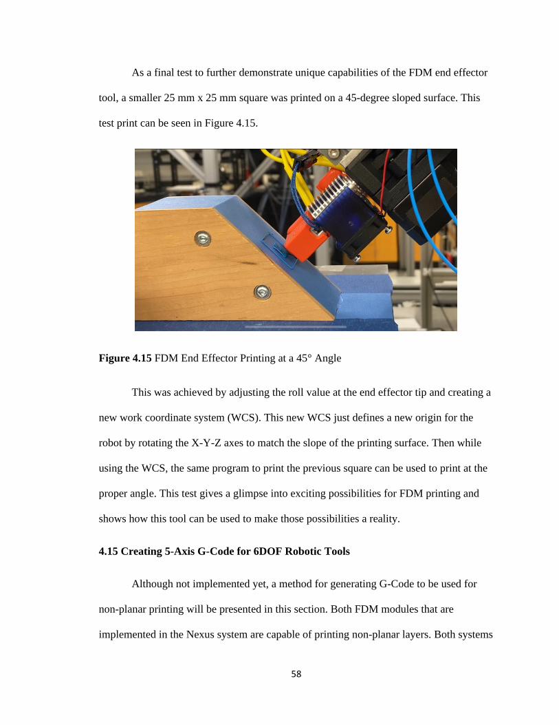
58

As a final test to further demonstrate unique capabilities of the FDM end effector

tool, a smaller 25 mm x 25 mm square was printed on a 45-degree sloped surface. This

test print can be seen in Figure 4.15.

Figure 4.15 FDM End Effector Printing at a 45° Angle

This was achieved by adjusting the roll value at the end effector tip and creating a

new work coordinate system (WCS). This new WCS just defines a new origin for the

robot by rotating the X-Y-Z axes to match the slope of the printing surface. Then while

using the WCS, the same program to print the previous square can be used to print at the

proper angle. This test gives a glimpse into exciting possibilities for FDM printing and

shows how this tool can be used to make those possibilities a reality.

4.15 Creating 5-Axis G-Code for 6DOF Robotic Tools

Although not implemented yet, a method for generating G-Code to be used for

non-planar printing will be presented in this section. Both FDM modules that are

implemented in the Nexus system are capable of printing non-planar layers. Both systems

59

can change the angle between the nozzle and the printing surface, which is key to

avoiding collisions while printing non-planar layers. Traditional printing happens one

layer at a time and the Z-height does not change until the previous layer is complete;

however, non-planar printing can vary the Z-height while moving in the X-Y plane. This

allows 3D prints to have a much smoother, uniform surface compared to the “stair-

stepping” effect that is seen with traditional printing methods. Figure 4.16 shows the

difference in surface finish that can be achieved with non-planar printing when compared

with traditional printing.

Figure 4.16 (Left) Stair-stepping effect from Traditional Printing, (Right) Non-planar

Print [32]

Non-planar printing can actually be realized using Cartesian machines, but it is

not optimized. This is because regular Cartesian 3D printers have no way of changing the

angle between the nozzle and the printing surface. This means that if the toolpath is

climbing or descending a slope too steep, the side of the nozzle will collide with the

already deposited material [30]. The solution to this is to provide a way to rotate the

60

nozzle around two different axes. As mentioned previously, this functionality is available

on both FDM systems developed in this thesis. Since the functionality already exists, the

only remaining problem is software based. The problem to solve now is how to generate

a toolpath that adds rotations.

The method proposed is to continue utilizing G-Code but add rotations of I and J

at the end of each line that contains movement commands. I and J represent the rotations

about the X and Y axis respectively. This format of this G-Code is called “5-Axis G-

Code” and is commonly seen used with CNC machines. This format will make it very

easy to add rotation functionality to the already existing LabVIEW control software that

was created for the FDM End Effector. The only remaining problem to solve is how to

generate G-Code in this format. This requires software that does not exist. A thesis from

the University of Hamburg showed that existing open-source Slicer software can be

modified to generate toolpaths that vary the Z-height when moving along the X-Y plane

in order to print curvilinear surfaces, but these paths did not include rotations and were

only demonstrated on Cartesian machines [31]. It is probably possible to continue this

work and add rotations based on the optimal angle at each coordinate point along the

toolpath. The optimal angle would be some angle that keeps the nozzle tip of the hotend

perpendicular to the printing surface (print bed or previous layer).

Another possible method might be to use software made for CAM that already

has methods of generating 5-Axis G-Code and creating a toolpath and then reversing it.

These toolpaths are made to subtract material from starting material, but it might be

possible to use them in reverse for additive manufacturing.

61

The last possible method would be to use MATLAB to figure out how to generate

optimal toolpaths for the 3D print. An STL file is made up of thousands of small triangles

with coordinates attached to them. Importing these into MATLAB into a large array, a

method could be developed to build a base layer and then analyze the outside surfaces to

determine when to stop printing planar layers, and start printing conformally, so that the

finished print has a smooth, conformal surface.

4.16 Summary

The stationary FDM module was successfully designed and integrated into the

Nexus system. Components were selected to help facilitate integration into the Nexus

system. Dual Diabase extruders were setup with a custom mount to allow them to attach

to the Nexus system’s aluminum extrusions. All controls were wired to a custom control

box that is mounted on the side of the aluminum extrusion profile, right next to the

extruders. A Smoothieboard controls the extrusion process of the 3D printing while the

motion of the printing stage is achieved using a Newport controller in LabVIEW. These

controllers are synchronized in LabVIEW using G-Code. Furthermore, a simple process

was developed to go from CAD to 3D print by importing an STL into the open-source

slicing software, “PrusaSlicer” and then sending the generated G-Code to a custom

LabVIEW program that synchronizes the extrusion of material with the movement of the

6-DOF positioner. In the latter part of the chapter, the principles learned from the

stationary FDM module were applied to develop a more customized 3D printer for a

robotic arm.

A FDM End Effector was designed from the ground up in CAD to be completely

self-contained and a prototype was fabricated and tested. A custom 3D printing firmware

62

was developed in LabVIEW and functionality of the tool and the software was tested

when attached to a robotic arm. All functions worked successfully, and a test print was

performed to further demonstrate the capabilities of the tool. The design incorporates

many desired features for an FDM 3D printer into a small and compact tool that can be

used with any robotic manipulator that uses the same ATI toolchanger. Dual nozzles

allow for multi-material or multi-resolution printing while the direct drive extruders

allow superior performance and can print any filament, flexible or stiff, all the way up to

300 °C. This tool also manages to contain all the components on the tool itself, whereas

most other FDM end effectors do not. The extruders can be individually actuated, so they

can be moved up out of the way when not in use. This will be useful for printing non-

planar layers in the future. Finally, non-planar printing was discussed and three methods

to achieve non-planar 3D printing using the Nexus system were proposed.

63

CHAPTER V

CONCLUSION

The field of additive manufacturing is still making a lot of progress and the Nexus

system offers unique process capabilities by using robotics to automate and combine

additive processes. This work discussed the development of two FDM systems and an

AJP system that are integrated into the Nexus system. Chapter 1 began by introducing the

motivation behind the work and sharing the associated challenges with integrating each

of these systems. It also shared details about the work contributed and a quick overview

of the organization of this thesis. Chapter 2 provided background information on each

technology mentioned in this work including: FDM, AJP, strain gauges, IPL, and the

Nexus system. Chapter 3 is all about the development of AJP processes as well as curing

methods. It begins discussing the first conference paper published that characterized

Clariant ink and curing using an oven. It shares methods of measuring conductivity using

the Van der Pauw four point probe station and then transitions into the second conference

paper published that characterizes NovaCentrix silver ink and shares the development

and analysis of a printable strain gauge. The chapter ends discussing progress made to

transition curing methods from the oven to IPL. Chapter 4 details the work of integrating

the stationary FDM module into the Nexus system as well the process necessary to go

from CAD design to complete 3D print. The remaining part of chapter 4 shares the design

philosophy of the FDM end effector tool and provides details for the mechanical,

electrical, and software portions of the prototype. The chapter also discusses non-planar

64

printing and offers some recommended methods for generating 5-Axis G-Code that can

be used to achieve non-planar printing without collisions.

65

REFERENCES

1. S. Scott Crump, “Apparatus and Method for Creating Three-Dimensional Objects,”

U.S. Patent 5,121,329, Jun. 9, 1992

2. M. Maher, A. Smith, and J. Margiotta, A synopsis of the Defense Advanced Research

Projects Agency (DARPA) investment in additive manufacture and what challenges

remain (SPIE LASE). SPIE, 2014.

3. N. J. Wilkinson, M. A. A. Smith, R. W. Kay, and R. A. Harris, "A review of aerosol jet

printing—a nontraditional hybrid process for micro-manufacturing," The International

Journal of Advanced Manufacturing 6 © 2019 by ASME Technology, vol. 105, no. 11,

pp. 4599-4619, 2019/12/01 2019, doi: 10.1007/s00170-019-03438-2.

4. OPTOMEC, "AEROSOL JET PRINTED ELECTRONICS OVERVIEW."

5. T. Rahman, L. Renaud, D. Heo, M. Renn, and R. Panat, "Aerosol based direct-write

micro-additive fabrication method for sub-mm 3D metal-dielectric structures," Journal of

Micromechanics and Microengineering, vol. 25, no. 10, p. 107002, 2015.

6. K. K. Christenson, J. A. Paulsen, M. J. Renn, K. McDonald, and J. Bourassa, "Direct

printing of circuit boards using Aerosol Jet®," in NIP & Digital Fabrication Conference,

2011, vol. 2011, no. 2: Society for Imaging Science and Technology, pp. 433-436.

7. M. Hedges and A. B. Marin, "3D Aerosol jet printing- Adding electronics functionality

to RP/RM," in DDMC 2012 conference, 2012, pp. 14-15.3.

8. K. Schuetz, J. Hörber, and J. Franke, "Selective light sintering of Aerosol-Jet printed

silver nanoparticle inks on polymer substrates," in AIP Conference Proceedings, 2014,

vol. 1593, no. 1: American Institute of Physics, pp. 732-735.

9. A. Shankar, E. Salcedo, A. Berndt, D. Choi, and J. E. Ryu, "Pulsed light sintering of

silver nanoparticles for large deformation of printed stretchable electronics," Advanced

Composites and Hybrid Materials, vol. 1, no. 1, pp. 193-198, 2018.

10. National Instruments (1998). Strain Gauge Measurement – A Tutorial (Application

Note 078).

11. Beckwith, T.G., Buck, N.L. and Roy, D., Marangoni. 1982. Mechanical

Measurements. Chapter 9.

12. Schroder KA, McCool S Cand Furlan WF 2006 Broadcast photonic curing of metallic

nanoparticle films Proc. NSTI Nanotechnology Conf. (3 May 2006) vol 198 p 201

66

13. Zenou M et al 2014 Laser sintering of copper nanoparticles J. Phys. D: Appl. Phys.

47 025501

14. Ali Roshanghias et al, “Sintering strategies for inkjet printed metallic traces in 3D

printed electronics,” 2017 Flex. Print. Electron. 2 045002

15. Wei, D, Trombley, C, Sherehiy, A, Popa, D. “Precise and Effective Robotic Tool

Change Strategy Using Visual Servoing with RGB-D Camera.” Proceedings of the ASME

2021 International Design Engineering Technical Conferences and Computers and

Information in Engineering Conference. Virtual, Online. August 17-20, 2021. ASME.

16. Wei, D, Tofangchi, A, Sherehiy, A, Saadatzi, MH, Alqatamin, M, Hsu, K, Popa, D.

“Precision Evaluation of Nexus, a Custom Multi-Robot System For MicroSystem

Integration.” Proceedings of the ASME 2021 16th International Manufacturing Science

and Engineering Conference. Volume 2: Manufacturing Processes; Manufacturing

Systems; Nano/Micro/Meso Manufacturing; Quality and Reliability. Virtual, Online. June

21–25, 2021. ASME.

17. Ratnayake, D, Curry, AT, Qu, C, Usher, J, & Walsh, K. "Characterizing the

Conductivity of Aerosol Jet Printed Silver Features on Glass." Proceedings of the ASME

2021 16th International Manufacturing Science and Engineering Conference. Volume 2:

Manufacturing Processes; Manufacturing Systems; Nano/Micro/Meso Manufacturing;

Quality and Reliability. Virtual, Online. June 21–25, 2021. V002T08A007. ASME.

18. A. Kamyshny, J. Steinke, and S. Magdassi, "Metal based inkjet inks for printed

electronics," The Open Applied Physics Journal, vol. 4, no. 1, 2011.

19. L. Makkonen, "On the Methods To Determine Surface Energies," Langmuir, vol. 16,

no. 20, pp. 7669-7672, 2000/10/01 2000, doi: 10.1021/la990815p.

20. O. Philips’Gloeilampenfabrieken, "A method of measuring specific resistivity and

Hall effect of discs of arbitrary shape," Philips Res. Rep, vol. 13, no. 1, pp. 1- 9, 1958.

21. D. Ratnayake, A. Curry and K. Walsh, "Demonstrating a new ink material for aerosol

printing conductive traces and custom strain gauges on flexible surfaces," 2021 IEEE

International Conference on Flexible and Printable Sensors and Systems (FLEPS), 2021,

pp. 1-4, doi: 10.1109/FLEPS51544.2021.9469773.

22. Whitefoot, J., Use of Strain Gages to Determine the Strain in Cantilever Beams.

2018.

23. Philips’ Gloeilampenfabrieken, O., A method of measuring specific resistivity and

Hall effect of discs of arbitrary shape. Philips Res. Rep, 1958. 13(1): p. 1-9.

24. Amir Hossein Ghahremani, “Rapid Annealing of Perovskite Solar Cell Thin Film

Materials Through Intense Pulse Light,” 2021 University of Louisville, Ph.D Dissertation

67

25. N. Shahrubudin, T.C. Lee, R. Ramlan, An Overview on 3D Printing Technology:

Technological, Materials, and Applications, Procedia Manufacturing, Volume 35, 2019,

Pages 1286-1296, ISSN 2351-9789

26. Fawaz Alabdullah, “Fused Deposition Modeling (FDM) Mechansim,” International

Journal of Scientific & Engineering Research, Vol. 7, Issure 5, 2016.

27. V. Surange, P. Gharat, “3D Printing Process Using Fused Deposition Modeling

(FDM),” 2016 Interntational Research Journal of Engineering and Technology (IRJET)

vol 03 issue 03

28. Yoon, YJ, Yon, M, Jung, SE, & Gupta, SK. "Development of Three-Nozzle

Extrusion System for Conformal Multi-Resolution 3D Printing With a Robotic

Manipulator." Proceedings of the ASME 2019 International Design Engineering

Technical Conferences and Computers and Information in Engineering Conference.

Volume 1: 39th Computers and Information in Engineering Conference. Anaheim,

California, USA. August 18–21, 2019. V001T02A024. ASME.

29. BCN3D Technologies (2019). The anatomy of an Extrusion System – How BCN3D

has partnered with industry-leading manufacturers to get the most productive 3D

printers. (Whitepaper).

30. Shembekar, A, Yoon, Y, Kanyuck, A, Gupta, S, “Generating Robot Trajectories for

Conformal Three-Dimensional Printing Using Nonplanar Layers,” Journal of Computing

and Information Science in Engineering, vol 19, Sept. 2019. ASME.

31. Daniel Ahlers, “3D Printing of Nonplanar Layers for Smooth Surface Generation,”

2018 University Of Hamburg, Master’s Thesis.

32. Waktin, Hanna, “Nonplanar 3D Printing Givers Curvy Top Layers”,

https://all3dp.com/4/nonplanar-3d-printing-gives-the-smoothest-top-layers/. 2019

68

APPENDIX A

To generate G-Code to 3D print using the Nexus system, PrusaSlicer is used.

Once open, select File>Import to import an STL file. On the right side, click on Expert to

show all possible settings in the other tabs. First, click on the Printer Settings tab and then

click on General and “Set” next to Bed shape. Select Rectangular and set the size and

origin. Make sure the origin is in the center of the bed.

Figure A-1 PrusaSlicer Print Bed Settings

69

Then click on the Print Settings tab and click on “Speed”. Set all speeds to 30 mm/s.

Figure A-2 Printing Speed Settings

Then under the Filament Settings tab, set the bed temperature to 0 °C and then set the

extruder temperature based off of the filament being used (about 205 °C for PLA). The

remaining settings can determined by the user. Once done click on “Preview” in the

bottom left to slice the model and then on “Export G-Code” in the bottom right.

70

Figure A-3 Slice Model and Export G-Code

71

APPENDIX B

This guide will demonstrate how to generate G-Code for the Nexus system’s

Aerosol Jet Printer using Fusion 360. This guide will use Autodesk’s Fusion 360

Education Version. A sketch can either be created in the “Design” workspace, or

imported from a .DXF file. Remember that each sketch line will represent the center of a

printed trace. Therefore, when creating a design, the desired trace width must be kept in

mind.

Figure B-1 DXF file imported into Fusion 360

72

Once the sketch or .DXF is finalized, switch to the “Manufacture” workspace by clicking

in the top left. Then select “Setup” (just to the right of “Manufacture”) and under

Operation Type select “Cutting”. If the setup did not automatically select the sketch

model, you can select it at the bottom of the setup menu. Once the model is selected,

setup the origin using the Work Coordinate System settings. For the Nexus system, the

center of the design is usually used as the origin, although for some special alignment

cases, this can change.

Figure B-2 Manufacturing Workspace (CAM) Setup For Fusion 360

After the setup is complete, select “Cutting > 2D-profile” from the top toolbar. A menu

should pop-up at this point. Under the first tab, click on “Select tool”. This will open the

Fusion 360 tool library where we will add a tool to use for the Optomec. Click on the +

73

sign in the top toolbar to add a new tool. Scroll down and select “Waterjet” as the type of

tool to add. Under the General tab, put “Optomec 50 um Traces” for the description and

“Optomec” for the Vendor. Under the Cutter tab, select millimeters for the units and put

0.05 mm for the kerf width and 3 mm for the nozzle clearance diameter. Skip over to the

Cutting Data tab and select ‘machine uses feeds” for the quality control. Then for cutting,

lead-in, and lead-out feedrate, set all of them to 600 mm/min. This will correspond to 10

mm/sec necessary for the NovaCentrix ink. Leave all other settings as default and click

accept when you are finished. You only need to create the tool once, next time you will

just select it from your library.

Now that the tool has been created, go to the second tab of the 2D profile,

geometry. Click the box next to contour selection and then select your sketch from the

left browser pane. Then set the remaining tabs to the same settings you see in Figure B-4.

74

Figure B-3 Select the Sketch as the Geometry to Print

Figure B-4 Remaining Settings for Profile

75

Once all settings are selected, click ok to finish. If you ever need to go back and

edit the settings, you can right click the 2D profile under the browser pane on the left and

select edit to return to this menu. Right clicking on the 2D profile also gives the option to

simulate the operation, which should always be done to make sure no mistakes were

made. To export the toolpath as G-Code, select the setup in the left browser pane and

then select “Post Process” from the top toolbar. For the post, select

“DITCNC_RepRapFW.cps”, which can be found on Cardbox. Then click on “Post” to

generate a G-Code file. Finally, open the G-Code file and make sure all feedrates are at

600.

Figure B-5 Post Process to Generate G-Code for Nexus

76

APPENDIX C

This appendix will share screenshots of the LabVIEW 3D Printing Firmware developed

for the FDM End Effector.

Figure C-1 3D Printer UI for FDM End Effector

The LabVIEW VI has three main loops: Denso robot movement, G-Code interpreter, and

a PID controller for the hotend. There is also a sub-VI to move the stepper motor attached

to the extruder

77

Figure C-2 Main-VI Loop to move Denso 6-DOF arm based on G-Code

Figure C-3 Main-VI Loop that Interprets G-Code and Sends Information to Other Loops

78

Figure C-4 Main-VI Loop Containing PID Controller to Control Hotend

Figure C-5 Sub-VI to Control Stepper Motor that Moves Extruder

79

CURRICULUM VITAE

Alexander Thomas Curry

LARRI at University of Louisville

2210 S Brook St, Louisville, KY 40208

DOB

Louisville, Kentucky – February 21, 1997

Education

2015-2019…………………………B.S.E., Engineering Physics, Murray State University

2020-2021………………………....M.S., Electrical Engineering, University of Louisville

Conference Publications

1) Ratnayake, D, Curry, AT, Qu, C, Usher, J, & Walsh, K. "Characterizing the

Conductivity of Aerosol Jet Printed Silver Features on Glass." Proceedings of the ASME

2021 16th International Manufacturing Science and Engineering Conference. Volume 2:

Manufacturing Processes; Manufacturing Systems; Nano/Micro/Meso Manufacturing;

Quality and Reliability. Virtual, Online. June 21–25, 2021. V002T08A007. ASME.

2) D. Ratnayake, A. Curry and K. Walsh, "Demonstrating a new ink material for aerosol

printing conductive traces and custom strain gauges on flexible surfaces," 2021 IEEE

80

International Conference on Flexible and Printable Sensors and Systems (FLEPS), 2021,

pp. 1-4, doi: 10.1109/FLEPS51544.2021.9469773.

Skills

• PCB Design

• C/C++

• Digital/Analog IC Design

• CAD/CAM Design

• Additive Manufacturing

• Machining

• Electrical Testing

Software

• Altium Designer

• LabVIEW

• MATLAB

• Fusion 360 CAD/CAM

• L-Edit

• Xilinx

• Microsoft Office