arX

iv:1

205.

6974

v1 [

cs.IT

] 31

May

201

21

The Porosity of Additive Noise SequencesVinith Misra and Tsachy Weissman,Senior Member, IEEE

Abstract

Consider a binary additive noise channel with noiseless feedback. When the noise is a stationary and ergodic processZ, thecapacity is1−H(Z) (H(·) denoting the entropy rate). It is shown analogously that when the noise is a deterministic sequencez

∞,the capacity under finite-state encoding and decoding is1 − ρ(z∞), whereρ(·) is Lempel and Ziv’s finite-state compressibility.This quantity is termed theporosityσ(·) of an individual noise sequence. A sequence of schemes are presented that universallyachieve porosity for any noise sequence. These converse andachievability results may be interpreted both as a channel-codingcounterpart to Ziv and Lempel’s work in universal source coding, as well as an extension to the work by Lomnitz and Feder andShayevitz and Feder on communication across modulo-additive channels. Additionally, a slightly more practical architecture issuggested that draws a connection with finite-state predictability, as introduced by Feder, Gutman, and Merhav.

Index Terms

Lempel-Ziv, universal source coding, universal channel coding, modulo-additive channel, compressibility, predictability

I. I NTRODUCTION

The “core” results of information theory, starting with Shannon’s source and channel coding theorems, are concernedwith probabilistic systems of a known model: an iid Bernoulli(1/4) source must be compressed, or perhaps bits are to becommunicated across an AWGN channel of known SNR. One may seek additional generality by asking that a coding schemesimultaneously function for an entire class of such probabilistic models. In the case of source coding, Ziv and Lempel [1],[2] and Ziv [3] take this question to its logical extreme and ask that a compressor not only achieve the optimal rate for anyprobabilistic source model, but do so forany individual source sequence. In [2], it is discovered that the traditionally relevantprobabilistic measurement — entropy rate — generalizes into a measure for an individual sequence — compressibility. Inthispaper, an analogous set of questions yield an analogous set of answers in the context of noisy channel coding with feedback.

Historically, far more attention has been paid to the issue of universality in source coding than in channel coding. The sourceof this discrepancy is readily apparent from Figs. 1 and 2. The encoder of Fig. 2 never observes the noise sequence in anyway, and so its codebook cannot be dynamically customized tosuit the channel. The source encoder of Figure 1 on the otherhand has direct access to the source sequence and can therefore adjust to its statistics. As such, the degree of universality thatcan be requested in the classical channel-coding setup is far more restricted than in source coding. Certainly, this does notpreclude discussion of “universality,” but the term must take on a considerably looser meaning, as is discussed in Sec. II.

The playing field is considerably leveled by introducing a noiseless feedback link, as in Fig. 3. In particular, the modulo-additive channel of Fig. 4 allows for a clear and precise analogy to the universal source coding of Lempel and Ziv. To highlightsome of the parallels:

• Individual sequences. In the source coding setting, Lempeland Ziv replace the source random processX∞ with adeterministic sequencex∞. Here, the standard stochastic description of channel noise Z∞ is supplanted by a specificindividual sequencez∞.

• Finite state constraint. Lempel and Ziv ask the question: how well can a source encoder/decoder perform for a specificindividual sequence, if the engineer designing the encoder/decoderknows the sequence ahead of time? Clearly, if theencoder and decoder are unconstrained, this problem trivializes: one may design a decoder that, with absolutely no input

This work was supported in part by the NDSEG fellowship, the Stanford Graduate Fellowship, and the NSF SCOI center.V. Misra (email: vinith@stanford.edu), and T. Weissman (email: tsachy@stanford.edu) are with the Department of Electrical Engineering, Stanford University,

Stanford, CA 94305 USA.

Unknown SourceX∞

E D X∞

Fig. 1. The model for universal source coding. An unknown source is provided to an encoder, which must describe it to the decoder.

Unknown ChannelM∞ E D M∞xi yi

Fig. 2. The model for universal channel coding. A message must be communicated over an unknown channel.

2

Unknown ChannelM∞ E D M∞xi yi

z−1yi−1

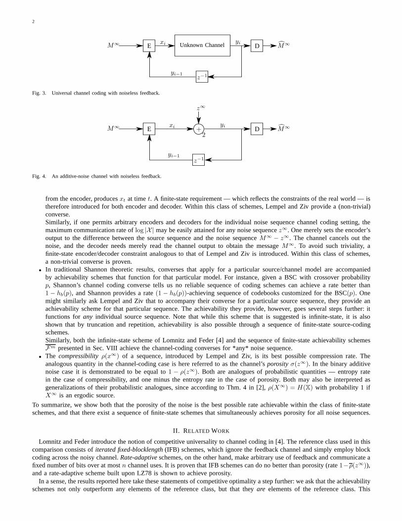
Fig. 3. Universal channel coding with noiseless feedback.

M∞ E D M∞xi yi

z−1yi−1

2

z∞

+

Fig. 4. An additive-noise channel with noiseless feedback.

from the encoder, producesxt at timet. A finite-state requirement — which reflects the constraintsof the real world — istherefore introduced for both encoder and decoder. Within this class of schemes, Lempel and Ziv provide a (non-trivial)converse.Similarly, if one permits arbitrary encoders and decoders for the individual noise sequence channel coding setting, themaximum communication rate oflog |X | may be easily attained for any noise sequencez∞. One merely sets the encoder’soutput to the difference between the source sequence and thenoise sequenceM∞ − z∞. The channel cancels out thenoise, and the decoder needs merely read the channel output to obtain the messageM∞. To avoid such triviality, afinite-state encoder/decoder constraint analogous to thatof Lempel and Ziv is introduced. Within this class of schemes,a non-trivial converse is proven.

• In traditional Shannon theoretic results, converses that apply for a particular source/channel model are accompaniedby achievability schemes that function for that particularmodel. For instance, given a BSC with crossover probabilityp, Shannon’s channel coding converse tells us no reliable sequence of coding schemes can achieve a rate better than1 − hb(p), and Shannon provides a rate(1 − hb(p))-achieving sequence of codebooks customized for the BSC(p). Onemight similarly ask Lempel and Ziv that to accompany their converse for a particular source sequence, they provide anachievability scheme for that particular sequence. The achievability they provide, however, goes several steps further: itfunctions forany individual source sequence. Note that while this scheme that is suggested is infinite-state, it is alsoshown that by truncation and repetition, achievability is also possible through a sequence of finite-state source-codingschemes.Similarly, both the infinite-state scheme of Lomnitz and Feder [4] and the sequence of finite-state achievability schemesFm presented in Sec. VIII achieve the channel-coding converses for *any* noise sequence.

• The compressibilityρ(x∞) of a sequence, introduced by Lempel and Ziv, is its best possible compression rate. Theanalogous quantity in the channel-coding case is here referred to as the channel’sporosityσ(z∞). In the binary additivenoise case it is demonstrated to be equal to1 − ρ(z∞). Both are analogues of probabilistic quantities — entropy ratein the case of compressibility, and one minus the entropy rate in the case of porosity. Both may also be interpreted asgeneralizations of their probabilistic analogues, since according to Thm. 4 in [2],ρ(X∞) = H(X) with probability 1 ifX∞ is an ergodic source.

To summarize, we show both that the porosity of the noise is the best possible rate achievable within the class of finite-stateschemes, and that there exist a sequence of finite-state schemes that simultaneously achieves porosity for all noise sequences.

II. RELATED WORK

Lomnitz and Feder introduce the notion of competitive universality to channel coding in [4]. The reference class used inthiscomparison consists ofiterated fixed-blocklength(IFB) schemes, which ignore the feedback channel and simplyemploy blockcoding across the noisy channel.Rate-adaptiveschemes, on the other hand, make arbitrary use of feedback and communicate afixed number of bits over at mostn channel uses. It is proven that IFB schemes can do no better than porosity (rate1−ρ(z∞)),and a rate-adaptive scheme built upon LZ78 is shown to achieve porosity.

In a sense, the results reported here take these statements of competitive optimality a step further: we ask that the achievabilityschemes not only outperform any elements of the reference class, but that theyare elements of the reference class. This

3

establishes porosity as a channel capacity of sorts. As IFB codes frequently cannot even achieve porosity for a given noisesequencez∞, let alone for the entire set of noise sequences, this requires that the reference class be widened to the class ofall finite-state schemes.

The porosity-achieving rate-adaptive scheme introduced by Lomnitz and Feder does not quite fall into this class, as it consistsof infinite states. One might consider consider truncating and repeating it in order to construct a finite state scheme. While thiscould potentially work, we find it somewhat easier to build from the schemes of Shayevitz and Feder [5], whose performanceguarantees mesh well with the asymptotic performance metrics of interest here.

In [5], Shayevitz and Feder establish the initial results that have sparked much of the subsequent work in this problem. Anextremely general family of channels is considered, but theresults provided are most meaningful when restricting attention tothe individual additive noise sequence setting. Of interest are two things: the construction of variable-rate, fixed-blocklengthschemes expanded from Horner’s coding method, and the strong performance guarantees that are provided. The schemes areshown to achieve for any noise sequence theempirical capacity, or one minus the first-order empirical entropy. By operatingthis coding technique overblocksof channel use, one can potentially generalize to arbitrary-order empirical entropies. Theachievability schemes{Fm} presented in this paper are an extension of this idea.

As with both [4] and [5], Eswaran et al. [6] consider a very broad class of channels with noiseless feedback, but theresults provided are most meaningful in the modulo-additive setting with an individual noise sequence. Extending [5],it isdemonstrated that even when the feedback is asymptoticallyzero-rate, the empirical capacity is still universally achievable.

As previously mentioned, even in the absence of a feedback link questions of universal channel coding can be considered.The principal complication in this setting is that the encoder no longer has any information about the specific channel, and soneither the rate nor the transmission methodology can be adapted.

One may nonetheless ask that thedecoderadapt to the channel. Csiszar and Korner [7] consider the class of memorylessDMC’s that share a common input alphabetX — call this classA(X ). For a randomly generated codebook, a universal decoderfor the entire classA(X ) is constructed and its performance compared to that of a decoder customized for whichever specificchannel happens to appear (maximum likelihood decoder). The universal decoder is not only shown to match the ML decoderin terms of vanishing error, but it is also found to achieve the same error exponent.

Ziv [8] and Lapidoth and Ziv [9] seek to expand such a result into the territory of channels with memory. Each considers afairly specific form of memory: finite-state channels with deterministic state transitions [8] and those with probabilistic statetransitions [9]. Each also demonstrates achievability through decoding schemes that utilize LZ78-style sequence parsing. Federand Lapidoth [10] on the other hand consider the more generalproblem of decoding for a parametric family of channels.

Despite the non-adaptability of the encoder in this feedback-less setting, one may seek to maximize the worst-case rateofcommunication across the channel. The fundamental limit ofperformance in this scenario is thecompound channel capacity,discussed at length in the review article by Lapidoth and Narayan [11].

A generalization of the above is to take a broadcast approach, wherein channel uncertainty is modeled by having the encoderbroadcast across all channels in the class considered. The rate region of this broadcast channel then characterizes therates theencoder may simultaneously achieve for each potential channel. Observe that if this rate region can be specifically determined,it answers all possible questions of universal decoding. Shamai and Steiner [12] leverage this approach for the case of fadingchannels.

III. STRUCTURE OFPAPER

In Sec. IV a precise description is provided of the problem setting, the class of finite-state schemes, and the relevantperformance metrics. Sec. V builds slightly on Lempel and Ziv’s definition of compressibility and establishes certain usefulproperties. Sec. VI states the three theorems that constitute the core results of this work. Sec. VII contains the proof of theconverse theorems, and Sec. VIII proves achievability. Sec. IX introduces a significantly more practical (but sub-optimal) setof schemes that establish a connection between porosity andfinite-state predictability. Sec. X summarizes this paper’s findings.A few lemmas have somewhat distracting proofs that are relegated to the appendices.

IV. PROBLEM SETUP

A deterministic additive noise feedback channel, as depicted in Fig. 4, is defined by a noise sequencez∞ ∈ X∞, whereXis a finite alphabet with a modulo-addition operator. The channel output at any timei is given by the sum of the noise andthe input:yi = xi + zi. Noiseless feedbackui = yi−1 delays the channel output by one time unit before providing it to theencoder. Without loss of generality, we will concern ourselves primarily with the binary-alphabet case, i.e.X = {0, 1}, as theextension to general finiteX is straightforward.

A. Finite-state Schemes

A finite-state (FS) encoder/decoder scheme for an additive noise channel — depicted in Fig. 5 — consists of severalcomponents:

1) An encoder state variables(e)i and decoder state variables(d)

i , each taking values in a finite setS.

4

M1, . . . ,Mpi,Mpi+1, . . . ,Mpi+ℓ︸ ︷︷ ︸,Mpi+ℓ+1, . . .

E D Mpi+Li−1pi

xi yi

z−1yi−1

2

z∞

+

θi

Fig. 5. A finite-state encoding/decoding scheme for a modulo-additive channel.

2) A source pointerpi and a finite lookahead constantℓ.3) An iid common randomness sourceθi ∼ pθ taking values in a finite alphabet.4) An encoding functionxi = e(s(e)

i ,Mpi+ℓpi

, yi, θi) ∈ X .5) A decoding length functionLi = dL(s

(d)i , yi, θi) that also determines the update of the source pointer:pi+1 = pi + Li.

6) A decoding functionMpi+Li−1pi

= dM (s(d)i , yi, θi).

7) State-update functions for both the encoders(e)i+1 = f(e)(s

(e)i ,Mpi+ℓ

pi, yi, θi) and decoders(d)

i+1 = f(d)(s(d)i , yi, θi).

At each time step, the encoding function determines the input xi to the channel, the decoding function estimates the firstLi source symbols that have yet to be estimated (based on the output yi of the channel), and state variables and the sourcepointer location are updated in anticipation of the next transmission.

Observe, first, that this class of schemes is sufficiently general to include the following as special cases:

1) The class of “iterated fixed-length” block schemes, as defined by Lomnitz and Feder [4]. These are simply block codesthat ignore the feedback. The common randomness at encoder and decoder allows for randomly generated block codesas well.

2) Schemes that transmit a variable number of source symbolsover a fixed number of channel uses, before reseting theirstate variables and repeating the operation (defined more precisely in Sec. VIII-A as “Repeated Finite-Extent” schemes).

3) Schemes that transmit a variable (or fixed) number of source symbols over a variable (but bounded) number of channeluses (also known as “rate-adaptive” schemes [4]).

Secondly, notice that without certain restrictions in the definition of class FS, the problem can become trivial:

1) Suppose that the encoder is permitted to be infinite-state. The system designer may then allow the encoder states(e)i

to be the current time indexi. This then allows the encoding function to be a function ofi, which in turn permits theencoding function to be customized for a particular noise sequencez∞: e(i,Mpi

) = Mpi− zi. Sending this through the

channel,zi is canceled out. The decoder needs merely read the channel output to obtain the message at the maximumpossible rate,log |X |.

2) Suppose that the decoder is permitted to be infinite-state. One may reverse the above construction by having the encoderblindly send the message bits through the channele(Mpi

) = Mpiand asking the decoder to cancel out the noise.

Specifically, lettings(d)i = i, the decoding function can be a function of the timei. This allows for a clever system

designer to choosedM (i, yi) = yi − zi, which guarantees thatMpi= Mpi

and thatLi = 1 for any i.3) Finally, suppose that the finite-lookahead requirement is nonexistant — that is, the encoding function can look at theentire

untransmitted message streamxi = e(s(e)i ,M∞

pi, yi, θi). As we will illustrate, this is identical to allowing the encoder an

infinite number of states. IfM∞ is a Bernoulli(1/2) sequence, then with probability one there exists a one-to-one mapbetweenM∞

i andi. The encoder may therefore sende(M∞pi) = Mpi

+ zpias the channel input at timei. The decoder,

as before, simply reads the channel output, achieving the maximum ratelog |X |.

B. Performance metrics

Channel coding typically concerns itself with the tradeoffbetween rate of communication and the frequency of errors. Inthe individual sequence setting of interest to us, we define the instantaneous rate and bit-error rate of an FS scheme at timenas

Rn =1

n

n∑

i=1

Li,

and

ǫn =1

nRn

nRn∑

i=1

1Mi 6=Mi

.

5

We consider two interpretations of these quantities.Best-Case. An FS schemebest-casep-achievesrate/error(R, ǫ) for a noise sequencez∞ if with at least probabilityp there

exists a sequence of points{ni} ∈ Z+ such thatlimi→∞ Rni

≥ R andlimi→∞ ǫni≤ ǫ. In other words, a performance monitor

that observes the system at the “right” times will see it achieve (R, ǫ) with probability at leastp. If p is 1, we say that thescheme simplybest-case achieves(R, ǫ).

Worst-Case. An FS schemeworst-casep-achievesrate/error(R, ǫ) if with at least probabilityp both lim infn→∞ Rn ≥ Rand lim supn→∞ ǫn ≤ ǫ. In other words, a performance monitor observing the systemat any set of sample times will see itachieve(R, ǫ) with probability at leastp. If p is one the scheme is said toworst-case achieve(R, ǫ).

Observe that the randomness in these definitions has two possible sources: the source sequenceM∞ and the common-information sequenceθ∞ used by the FS scheme. Sometimes the sourceM∞ will be a fixed sequence, but this is alwaysmade clear from context.

V. NOTIONS OF“ COMPRESSIBILITY”

The results of this paper connect the operational notions ofachievability to certain long-established individual sequenceproperties, first introduced by Lempel and Ziv [2] in a source-coding context. In this section, these properties are defined andsome useful relations are presented between them.

First, we denote thekth order block-by-block empirical distribution

pk(Xk)[xn] =1

⌊nk ⌋

⌊n/k⌋∑

i=0

1xk(i+1)ki+1 =Xk .

If the empirical distribution is instead computed in a sliding-window manner, we denote

pksw(Xk)[xn] =

1

n− k + 1

n−k+1∑

i=0

1xi+ki+1=Xk .

The argument[xn] is occasionally omitted when the context is clear.Thekth order block-by-block empirical entropy is indicated byHk(xn) = Hpk(Xk). The sliding-windowkth order empirical

entropy is similarly written asHksw(x

n) = Hpksw(Xk).

As shown by Ziv and Lempel [2], the finite-statecompressibilityof a sequencex∞ may be written as

ρ(x∞) = lim supk→∞

lim supn→∞

Hksw(x

n).

An analagous quantity may also be introduced:

ρ(x∞) = lim infk→∞

lim infn→∞

Hksw(x

n).

Operationally, compressibility is the smallest limit supremum compression ratio achievable for a sequence (Theorem 3in [2]).It is not difficult to show that, analogously, the second quantity is the smallest possible limit infimum compression ratio.Informed by this, we refer to the original compressibility quantity as theworst-case compressibilityand the new limit infimumversion as thebest-case compressibility.

The following lemma, proved in Appendix A, demonstrates that both best-case and worst-case compressibilities may becomputed using either block-by-block or sliding-window empirical entropies.

Lemma 1:Let x∞ be a finite-alphabet sequence. Then

ρ(x∞) = limk→∞

lim infn→∞

1

kHk(xn)

and

ρ(x∞) = limk→∞

lim supn→∞

1

kHk(xn).

The porosityof a noise sequencez∞ ∈ Z∞ is defined in best-case

σ(z∞) = log2 |Z| − ρ(z∞)

and worst-caseσ(z∞) = log2 |Z| − ρ(z∞)

varieties as well. Observe the sign changes: while a “good” compressibility is small, a “good” porosity is large. The remainderof this paper clarifies the operational significance of thesequantities.

6

VI. STATEMENT OF RESULTS

The results of this paper may be summarized as follows:

1) A converse that upper-bounds the best-case achievable rate by an FS scheme.2) A converse that upper-bounds the worst-case achievable rate by an FS scheme.3) A sequence of universal FS schemes{Fm}∞m=1 that simultaneously achieve the best-case and worst-case converse bounds

for any noise sequencez∞.

Formally, each of these three statements corresponds to a theorem:Theorem 2:Suppose an FS scheme best-casep-achieves(R, ǫ). If p > 0, then

R ≤ hb(ǫ) + σ(z∞).

Theorem 3:Suppose an FS scheme worst-casep-achieves(R, ǫ). If p > 0, then

R ≤ hb(ǫ) + σ(z∞).

Theorem 4:There exists a sequence of schemesFm, which for an iid Bernoulli(1/2) sourceM∞ and every noise sequencez∞ best-case achieves

σ(z∞)− δm(z∞) , ǫm/(σ(z∞)− δm(z∞)),

and worst-case achievesσ(z∞)− δm(z∞) , ǫm/(σ(z∞)− δm(z∞)),

with probability one, whereǫm, δm, andδm all go to zero.Theorems 2 and 3 are proven in Section VII. In Section VIII, weintroduce the schemes{Fm}∞m=1 and prove Theorem 4.

VII. PROOF OFCONVERSE

A. Definitions and Lemmas

In order to prove the converse theorems, a series of definitions and lemmas is first required.Lemma 5: (Selection Lemma) SupposeX∞ is iid Bernoulli(1/2) andL is a random positive integer with arbitrary conditional

distributionpL|X∞ with respect toX∞. ThenH(XL) ≥ E [L].Proof:

H(XL) =∑

xl

p(XL = xl) log1

p(XL = xl)

(a)

≥∑

xl

p(XL = xl) log1

p(X l = xl)

(b)

≥∑

xl

p(XL = xl)l

= E [L]

where step (a) follows because ifXL = xl thenX l must necessarily equalxl. Step (b) follows from the iid Bernoulli(1/2)distribution ofX∞.

Definition 1: Let {Li}∞i=1 be a bounded sequence of nonnegative integers, and letM∞ and z∞ as usual denote binarysequences. Thek-partition of (M∞, z∞) according to{Li} is the sequence of blocks

(MLi , zk)i = M∑

ij=1 Lj

∑i−1j=1 Lj+1

, zik(i−1)k+1.

In this context,{Li} are referred to as the partition lengths.Definition 2: Let x∞ be a sequence of symbols drawn from a finite alphabetX . If there exists a series of sample points

{ni}∞i=1 such that the sequencep1(x)[xni ] converges to a distributionp(x), p(x) is said to be a limiting distribution forx∞.Observe that for any finite-alphabet sequencex∞ at least one limiting distribution exists:p1(x)[xn] is an infinite sequence ina compact set, so at least one convergent subsequence must exist.

Definition 3: Let z∞ be a finite-alphabet sequence. The setMk(z∞) consists of all binary sequencesM∞ such that there

exist partition lengths{Li}, a resultingk-partition {(MLi, zk)i}, and a limiting distributionp(L,ML, zk) for the sequence{Li, (M

Li, zk)i} such thatE [L]p > Hp(M

L|zk) + 1. (1)

We may interpret the set in the following manner. Suppose first that a “genie” partitions the source sequenceM∞ intoan arbitrary series of variable-length blocks{(MLi)i}. Each block(MLi)i, of length Li, is then source-coded with side

7

information(zk)i at average rate less thanHp(ML|zk)+1. The setMk(z

∞) consists of all source sequences that, in a sense,allow such a genie/side-information-source-coding setupto compress strictly better than one bit per source symbol. One wouldexpect that the occurrence of such a set is a rare event when the source is drawn iid Bernoulli(1/2). This is formalized withthe following lemma.

Lemma 6:Let z∞ be a fixed finite-alphabet sequence, and letM∞ be drawn from an iid Bernoulli(1/2) process. Then theprobability thatM∞ ∈ Mk(z

∞) is zero for allk.Proof: See Appendix B.

We may easily expand this lemma to allow for common randomness.Corollary 7: Let z∞ be a fixed binary sequence, letM∞ be drawn from an iid Bernoulli(1/2) process, and letθ∞ be a

finite-alphabet sequence of arbitrary distribution that isindependent ofM∞. Then the probability thatM∞ ∈ Mk((zi, θi)∞i=1)

is zero for anyk.Proof: First observe that Lemma 6 does not require thatz∞ be a binary sequence — only that it be of a finite alphabet.

As such, for a given sequenceθ∞ we may define the surrogatez-sequencez∞ = (zi, θi)∞i=1.

Applying Lemma 6 for this surrogate sequence, we have that for any fixed z∞ and θ∞, the probability of drawing anelement ofMk((zi, θi)

∞1 ) from a Bernoulli(1/2) process is zero. Sinceθ∞ is independent fromM∞, the corollary follows.

B. Converse Lemma

Although the converse results are presented as two distincttheorems, at their heart is the same argument. We present thiscore result in the following lemma.

Lemma 8:Suppose ans-stateℓ-lookahead FS scheme achieves(R, ǫ) on points{ni} for a specific source sequenceM∞,a specific channel noise sequencez∞, and a specific encoder/decoder common information sequence θ∞. If for somek ∈ Z

+

M∞ is not a member ofMk((zi, θi)∞i=1), and if Hk(zn) + Hk(θn)− Hk((zi, θi)

ni=1) →n→∞ 0, then

R ≤ 2 log s+ ℓ+ 2

k+ hb(ǫ) + 1− lim sup

i→∞

1

kHk(zni).

The general idea in proving this lemma is to turn any given FS scheme into asourceencoding/decoding scheme. Consideran FS decoder that achieves(R, ǫ) on some points{ni}, and ignore the minor complication of common randomnessθ∞. Givenonly the channel outputy∞, the decoder produces an estimate of the source sequenceM∞. Knowing the source sequenceand the channel output, the decoder is technically capable of “simulating” the encoder and thereby obtaining both the channelinput sequencex∞ and the noise sequencez∞. One may therefore interpret the channel outputy∞ as an encoding of the jointsource sequence(M∞, z∞). The following proof utilizes a rigorous argument inspiredby this intuition.

Proof: Let e∞ denote the error indication sequenceei = 1Mi 6=Mi. First, consider thek-partition of (M∞, z∞, θ∞, e∞)

according to the given FS scheme:

(MLi , eLi, zk, θk)∞i=1 =(Mpik+1−1

p(i−1)k+1, epik+1−1

p(i−1)k+1, zik(i−1)k+1, θ

ik(i−1)k+1

)∞i=1

.

In other words, let(MLi , eLi , zk, θk)i enumeratek-blocks of channel noise and common information, along withthe sourcebits that are estimated during each such block and the error indicators for these source bits. LetLi = pik+1−p(i−1)k+1 denotethe partition lengths.

Now define the sequence of points{n∗i } ⊂ {ni} so that

limi→∞

1

kHk(zn

∗

i ) = lim supi→∞

1

kHk(zni), (2)

and letp(ML, eL, zk, θk) be a limiting distribution of(ML, zk, θk)i on these points{n∗i }. Recall from Def. 2 that such a

limiting distribution always exists.Suppose random variables(ML, eL, zk, θk) are distributed according top(ML, zk, θk). We first use the FS scheme given

in the lemma statement to construct a lossless source encoder/decoder for(ML, zk), with θk as side information. By laterrequiring that the rate of this encoding exceedHp(M

L, zk|θk), the lemma may be proven.

E1 Letj ∈ Z+. We construct a codeword for the source block(MLj , zk)j given side information block(θk)j as follows:

1) To reduce clutter, we remove some of the unnecessary indices. Denote the source bits used by the FS encoderduring thisjth block asM ℓ = M

p(j−1)k+1+ℓ−1p(j−1)k+1 . Similarly, let the source bits estimated by the FS decoder be

referred to asML = Mpjk+1−1p(j−1)k+1

and the error indicators aseL = epjk+1−1p(j−1)k+1

. Additionally, let s(e) = s(e)(j−1)k+1

ands(d) = s(d)(j−1)k+1 indicate the initial encoder and decoder states, and letxk = xjk

(j−1)k+1 andyk = yjk(j−1)k+1denote the channel inputs and outputs during the block.

2) Apply a binary Huffman code toeL to create the compressed representationg(eL) ∈ {0, 1}∗. The Huffmancode is designed according to the limiting empirical distribution p(eL).

8

3) Add the codeword(s(e), s(d),ML+ℓL+1 , y

k, g(eL)) to the codebook.4) Observe that(s(e), s(d),ML+ℓ

L+1 , g(eL)) decodes uniquely into(ML, zk)j given side information block(θk)j :

• Simulate the channel decoding operation with initial states(d), common informationθk, and channel outputyk. This yieldsML. Correcting for errors with the correctional information embedded ing(eL), we haveML.

• Simulate the channel encoding operation using initial state se, feedbackyk, common informationθk, sourceML from the previous step, andML+ℓ

L+1 from the codeword. This yields the channel inputxk, which produceszk when modulo-2 added toyk.

Refer to this decoding operation on a codewordc asC−1(c, θk).

E2 Build the codebook by repeating stepE1 for every block(ML, zk, θk)j , j ∈ Z+. Note that each codeword is of

length2 log s+ ℓ+ k + length(g(eL)) and losslessly decodes into its source block. Call this codebook C.E3 Define the codebook encoding functionF of a source sample(ML, zk|θk) as mapping to the shortest codeword in

the set{c ∈ C : C−1(c, θk) = (ML, zk)}.

We now establish the expected length of this code when applied to the probabilistic source(ML, zk|θk). As mentioned instep E2, a given codeword is of length2 log s + ℓ + k + length(g(eL)), whereeL is the error sequence. According to theassumptions of the lemma, the bit error rate on points{n∗

i } is upper-bounded byǫ. From this and fromp(eL) being a limitingdistribution on{n∗

i }, the expected frequency of1 in eL may be upper-bounded byǫ. Therefore, the expected length ofg(eL)is upper-bounded bykhb(ǫ) + 1, and

E[length(F (ML, zk|θk))

]p≤ 2 log s+ ℓ+ k(1 + hb(ǫ)) + 1.

SinceF is a lossless variable-length encoder for sources drawn from p(ML, zk|θk), the expected codeword length mustexceed the conditional entropy according top:

2 log s+ ℓ+ k (1 + hb(ǫ)) + 1 ≥ Hp(ML, zk|θk)

≥ Hp(zk|θk) +Hp(M

L|zk, θk)(a)= Hp(z

k) +Hp(ML|zk, θk)

(b)

≥ Hp(zk) + E [L]p − 1

(c)= lim sup

i→∞Hk(zni) +Rk − 1

where (a) holds because of the final assumption in the theoremstatement, (b) follows from Corollary 7, and (c) is due to both(2) and the lemma’s assumption about rateR being achieved on points{n∗

i }. Rearranging terms proves the lemma.

C. Proof of Converses

Armed with Lemma 8, it is a relatively straightforward matter to prove Theorems 2 and 3.Proof of Theorem 2:We first note that becauseθ∞ is drawn iid andz∞ is fixed,Hk(zn)+ Hk(θn)− Hk((zi, θi)

ni=1) → 0

with probability one for everyk. Furthermore, by Corollary 7,M∞ /∈ Mk((zi, θi)∞i=1) with probability one for every k.

Therefore, if(R, ǫ) is best-case-achieved with positive probability, it must then be achieved for some specific(M∞, θ∞) suchthatM∞ /∈ Mk((zi, θi)

∞i=1 andHk(zn)+ Hk(θn)− Hk((zi, θi)

ni=1) → 0 for everyk. Let {ni} be the subsequence on which

it is achieved.Applying Lemma 8,

R ≤ 2 log s+ ℓ+√k

k+ hb(ǫ) + 1− 1

klim supi→∞

Hk(zni),

for any k.Taking the limit supremum ask → ∞,

R ≤ hb(ǫ) + 1− lim infk→∞

1

klim supi→∞

Hk(zni)

≤ hb(ǫ) + 1− lim infk→∞

1

klim infi→∞

Hk(zni)

≤ hb(ǫ) + 1− lim infk→∞

1

klim infn→∞

Hk(zn)

= hb(ǫ) + 1− ρ(z∞).

9

M1, . . . ,Mpi,Mpi+1, . . . ,Mpi+ℓ︸ ︷︷ ︸,Mpi+ℓ+1, . . .

E D Mpi+Li−1pi

xi yi

pui|yi−1,s(f)ui

2

z∞

+

θi

Fig. 6. A finite-state active feedback scheme for a modulo-additive channel.

Proof of Theorem 3:If (R, ǫ) is worst-case-achieved with positive probabilityp, then it must be worst-case achieved forsome(M∞, θ∞) such thatM∞ /∈ Mk((zi, θi)

∞i=1 (because by Corollary 7 this occurs with probability one) and Hk(zn) +

Hk(θn)− Hk((zi, θi)ni=1) → 0 (because this occurs with probability one whenθ∞ is chosen iid).

We may therefore apply Lemma 8 with{ni} = Z+. For anyk, we have that

R ≤ 2 log s+ ℓ+√k

k+ hb(ǫ) + 1− 1

klim supn→∞

Hk(zn).

Since this holds for arbitraryk, we may take the limit infimum of the expression withk → ∞:

R ≤ lim infk→∞

(2 log s+ ℓ+

√k

k+ hb(ǫ) + 1− 1

klim supn→∞

Hk(zn)

)

= hb(ǫ) + 1− lim supk→∞

1

klim supn→∞

Hk(zn)

= hb(ǫ) + 1− ρ(z∞).

VIII. P ROOF OFACHIEVABILITY

In this section, a sequence of FS schemes is constructed and guaranteed to achieve both the best-case and worst-case boundsfor any channel noise sequencez∞. This “universal achievability” is analogous to the universal source coding achievabilityscheme introduced by Ziv and Lempel [2].

A. Some Classes of Schemes

To begin, several additional classes of schemes are introduced, and their relationships with each other and with class FS areclarified. This will prove useful in constructing the universal achievability schemes.

A finite-state active feedback(FSAF) scheme is a variation of the class FS that allows for active feedback (Fig. 5). It consistsof the following:

1) An encoder state variables(e)i , a decoder state variables(d)

i , and a feedback state variables(f)i , all taking values in a finite

set.2) A source pointerpi and a finite lookahead constantℓ.3) An iid common randomness sourceθi ∼ pθ.4) A finite-state feedback channel whose output at timei is distributed according toUi ∼ pu|y,s(ui|yi, s(f)

i ).5) An encoding functionxi = e(s(e)

i ,Mpi+ℓpi

, θi, ui).6) A decoding length functionLi = dL(s

(d)i , yi, θi, ui) that also determines the update of the source pointer:pi+1 = pi+Li.

7) A decoding functionMpi+Li−1pi

= dM (s(d)i , yi, θi, ui).

8) State-update functions for the encoders(e)i+1 = f(e)(s

(e)i ,Mpi+ℓ

pi, θi, ui), decoders(d)

i+1 = f(d)(s(d)i , yi, θi, ui), and feedback

channels(f)i+1 = f(f)(s

(f)i , yi, θi).

Lemma 9:The class of schemes FSAF is equivalent to class FS.Proof: By settingUi = yi, we find that FS is a special case of FSAF. To show the other direction, first assume we are

given an FSAF scheme. By the arguments that follow, we will construct an FS scheme that simulates it. Quantities relatingtothe constructedFS scheme will be notated with a “hat,” e.g.θ, se

i, etc.First, letU be a random vector with components indexed byy ∈ X ands ∈ S(f) , and let the(y, s)th component be distributed

according toUy,s ∼ pU|y,s, wherepU|y,s is the given FSAF scheme’s feedback channel transition matrix. Furthermore, let thecomponents be independently distributed. We then define theFS scheme’s common randomness asθi = (θi,Ui) distributed

10

M∞ E D MLxi yi

pui|yi−1

ui

2

z∞

+

θ

Fig. 7. A finite-extent scheme.

iid according topθpU , wherepθ is the common randomness distribution for the given FSAF scheme. Let(Uy,s)i denote the(y, s)−th component of thei-th random vectorUi.

The equivalent FS scheme is assigned encoder and decoder state variabless(e)i = (s

(e)i , s

(f)i ) and s

(d)i = (s

(d)i , s

(f)i ), where

s(e)i , s(d)

i , ands(f)i are the state variables for the FSAF scheme. The encoder/decoder update functions are given by

f(e)(s(e)i ,Mpi+ℓ

pi, yi, θi) =

(f(e)(s

(e)i ,Mpi+ℓ

pi, θi, (Uyi,s

(f)i)i), ff(s

(f)i , yi, θi)

),

and

f(d)(s(d)i , yi, θi) =

(f(d)(s

(e)i , yi, θi, (Uyi,s

(f)i)i), ff(s

(f)i , yi, θi)

).

Observe how the randomness of the FSAF scheme’s active feedback channel is simulated by means of the common randomnessθi = (θi,Ui).

In this manner the FSAF encoder/decoder/feedback state machines are simulated by the FS encoder/decoder state machines.The FSAF encoding and decoding functions may be implementedin a similar manner:

e(s(e)i ,Mpi,pi+ℓ, yi, θi) = e(s(e)

i ,Mpi,pi+ℓ, θi, (Uyi,s(f)i)i),

and

dM (s(d)i , yi, θi) = dM (s(d)

i , yi, θi, (Uyi,s(f)i)i).

Since this constructed FS scheme is identical to the given FSAF scheme, FSAF is a special case of FS.A finite-extent(FEex) schemeF for a channel with alphabetX — as depicted in Fig. 7 consists of:

1) A extentn.2) A feedback channel with transition probabilities given by Ui ∼ pui

(ui|ui−1, yi) and taking values inX , for i ∈{1, . . . , n}.

3) A common randomness variableθ drawn from a finite alphabet, independent of the source, and provided to both encoderand decoder.

4) Encoding functionsx1 = e1(M∞, θ), x2 = e2(M

∞, θ, u1), . . . , xn = en(M∞, θ, un−1).

5) A decoding length functionL = dL(yn, θ, un−1), upper bounded byn log |X |.

6) A decoding functionML = dM (yn, θ, un−1).

A repetition schemeis constructed from ann-extent FE schemeF . Let F(M∞, zn) describe the application of schemeFto sourceM∞ and noise blockzn. Then the repetition schemeF consists of repeated independent uses ofF , i.e.

F(M∞, z∞) ≡{F ((Mn

1 , 0∞), zn1 ) ,F

((ML1+n

L1+1 , 0∞), z2nn+1

), . . .

}.

In each block,F is applied to a “virtual source” consisting of the firstn bits of the source that have yet to be transmitted anda string of 0s.

Proposition 10: The class of repetition schemes is a subclass of FSAF schemes(and therefore of FS schemes).This follows directly from two properties of repetition schemes:

• The block-based structure allows for implementation with finite-state machines.• A repetition scheme constructed from ann-extent FE scheme has finite lookahead constantn.

11

B. Universal Scheme Construction

At the core of the achievability scheme is a lemma, introduced and proven by Shayevitz and Feder [5]:Lemma 11:(Shayevitz and Feder, 2009) LetX be a finite alphabet with an addition operation. Then there exists a sequence of

n-extent FE schemesFn(X ) with the following worst-case performance guarantees overall additive noise sequencesz∞ ∈ X∞

and source sequencesM∞ ∈ {0, 1}∞

supzn∈Xn,M∞∈{0,1}∞

P(ML 6= ML

)≤ ǫ(n) (3)

and

infzn∈Xn,M∞∈{0,1}∞

P(L

n> 1− H1(zn)− ǫ(n)

)> 1− ǫ(n), (4)

whereǫ(n) → 0.Note that the only randomness in the above probabilistic statements is due to the randomness in the feedback channel.

Observe that Lemma 11 concerns itself with only the first-order empirical entropyH1(zn). By specializing to binarysequences, this may be replaced by higher-order empirical entropies.

Corollary 12: For binary additive noise channels with feedback, there exists a sequence of finite extent schemesFm withextentsN(m) → ∞ and the following performance guarantees:

supzN(m)∈XN(m),M∞∈{0,1}∞

P(ML 6= ML

)≤ ǫm

and

infzN(m)∈XN(m),M∞∈{0,1}∞

P(

L

N(m)> 1− 1

mHm(zN(m))− ǫm

)> 1− ǫm,

whereǫm → 0.Proof: For a givenm, consider them-tuple supersymbol channel characterized by inputsXi = xim

(i−1)m+1, noiseZi =

zim(i−1)m+1, and outputsYi = (x(i−1)m+1+z(i−1)m+1, x(i−1)m+2+z(i−1)m+2, . . . , xim+zim). Applying Lemma 11 to channelsof this alphabet yields a sequence of schemesFn({0, 1}m) with

ǫn,m →n→∞

0. (5)

Observe thatFn({0, 1}m) may be seen as a finite-extent scheme both for the supersymbolalphabet{0, 1}m additive noisechannel as well as for the (fundamental) binary alphabet{0, 1} additive noise channel.

By (5) we may chooseN(m) so thatǫN(m),m →m→∞

0. DenotingFm = FN(m)({0, 1}m), this proves the lemma.

The sequence of finite-extent schemes{Fm}∞m=1 form the basis of the universal achievability construction.Definition 4: The universal achievability scheme of orderm is the repetition schemeFm formed from theN(m)-extent

schemeFm.We end with an important lemma regarding repetition schemes.Lemma 13:Let F be anN -extent FE scheme and letF be the corresponding repetition scheme. DefineEi be the error

indicator for theith block and defineTi = 1Li≥aiso as to indicate if in theith block the number of bits transmitted exceeds

a fixed thresholdai. Then the Markov relationsEi −MN

(i) − Ei−1 (6)

andTi −MN

(i) − T i−1 (7)

both hold, whereMN(i) ≡ M

∑i−1j=1 Li+N

∑i−1j=1 Li+1

denotes theN source samples used in theith block by the repetition scheme.

Proof: See Appendix C.

C. Proving Achievability (Theorem 4)

Two additional lemmas, regarding the limiting behavior of random binary sequences, are required in order to prove thatFm

achieves the performance promised in Theorem 4.Lemma 14:Suppose{Xi} is a sequence of iid Bernoulli(p) random variables, and suppose{αi} is a bounded sequence of

real numbers. Then with probability one,

lim supn→∞

1

n

n∑

i=1

Xiαi = p lim supn→∞

1

n

n∑

i=1

αi

12

and

lim infn→∞

1

n

n∑

i=1

Xiαi = p lim infn→∞

1

n

n∑

i=1

αi.

Proof: Let Yi = αiXi. Sinceαi is bounded, there exists constantA such that|αi| < A. We then have thatE[Y 2i

]≤ A2 is

bounded and∑∞

k=11k2 varYi ≤ A2

∑∞k=1

1k2 < ∞. These two statements qualify the use of Kolmogorov’s strong law, which

states that1n∑n

i=1 Yi − 1n

∑ni=1 αip →

n→∞0 with probability one. This proves the lemma.

Lemma 15:Let {αi} be a bounded real-valued sequence, and let{Xi} be a random binary process. IfP(Xi = 1|X i−1 = xi−1

)≤

p for anyxi−1 ∈ {0, 1}i−1, then with probability one

lim supn→∞

1

n

n∑

i=1

αiXi ≤ pα (8)

lim infn→∞

1

n

n∑

i=1

αiXi ≤ pα (9)

whereα = lim supn→∞

∑ni=1 αi andα = lim infn→∞

∑ni=1 αi. Similarly, if P

(Xi = 1|X i−1 = xi−1

)≥ p for any xi−1 ∈

{0, 1}i−1,

lim supn→∞

1

n

n∑

i=1

αiXi ≥ pα (10)

lim infn→∞

1

n

n∑

i=1

αiXi ≥ pα (11)

Proof: Let {Yi} be a Bernoulli-p iid process. We will construct correlated binary processes{Xi, Yi} whose marginaldistributions are identical to those of{Xi} and{Yi}, and use these to prove the lemma.

• Let {Ui} be a sequence of independent uniform[0, 1] random variables.• For eachi let

Xi =

{1 if Ui < P

(Xi = 1|X i−1 = X i−1

)

0 otherwise

and

Yi =

{1 if Ui ≤ p0 otherwise

• By Lemma 14,lim supn→∞1n

∑ni=1 αiYi = pα and lim infn→∞

1n

∑ni=1 αiYi = pα.

• Consider the case whereP(Xi = 1|X i−1 = xi−1

)≤ p. Then sinceXi ≤ Yi we have that

lim supn→∞

1

n

n∑

i=1

αiXi ≤ pα

and

lim infn→∞

1

n

n∑

i=1

αiXi = pα

with probability one. Since{Xi} has the same marginal distribution as{Xi}, this proves (8) and (9).• Similarly, in the case whereP

(Xi = 1|X i−1 = xi−1

)≥ p, the relationXi ≥ Yi always holds and we have (10) and (11).

Proof of Theorem 4:SupposeFm is applied to a sourceM∞ and noise sequencez∞. Let {Li} be the number of

source bits decoded in each block. Consider theith block — i.e.F((M

∑i−1j=1 Li+N(m)

∑i−1j=1 Li+1

, 0∞), ziN(m)(i−1)N(m)+1

). Let MN(m)

(i) =

M∑i−1

j=1 Li+N(m)∑i−1

j=1 Li+1indicate the source bits used by the encoder, letMLi

(i) = M∑

ij=1 Li

∑i−1j=1 Li+1

indicate the estimate produced,

let Ri = Li

N(m) indicate the rate of the block, and letzN(m)(i) = z

iN(m)(i−1)N(m)+1 denote the noise of the block. Finally, let

uN(m)(i) = u

iN(m)(i−1)N(m)+1 denote the feedback during the block.

Rate Guarantees

13

Recalling thatǫm denotes the rate-error guarantee in Corollary 12, define the“rate indicator”Ti as the indication of whetherthe rate in theith block exceeds the threshold1− 1

mHm((zN(m)(i) ))− ǫm, i.e.

Ti = 1Ri≥1− 1

mHm((z

N(m)

(i)))−ǫm

. (12)

One may demonstrate that for anyi and anyti−1 ∈ {0, 1}i−1, P(Ti|T i−1 = ti−1

)≥ 1− ǫm:

P(Ti = 1|T i−1 = ti−1

)=

∑

mN(m)∈{0,1}N(m)

[P(Ti = 1|T i−1 = ti−1,M

N(m)(i) = mN(m)

)·

P(M

N(m)(i) = mN(m)|T i−1 = ti−1

)]

(a)=

∑

mN(m)∈{0,1}N(m)

[P(Ti = 1|MN(m)

(i) = mn)

P(M

N(m)(i) = mN(m)|T i−1 = ti−1

)]

(b)

≥ 1− ǫm, (13)

where step (a) follows from the Markov relation (Lemma 13) and step (b) is due to the rate guarantee in Corollary 12.Applying Lemma 15 to{Ti}, (10) bounds the limit supremum rate of the scheme.

lim supk→∞

1

k

k∑

i=1

Ri

(a)

≥ lim supk→∞

1

k

k∑

i=1

RiTi

(b)

≥ lim supk→∞

1

k

k∑

i=1

Ti

(1− Hm(z

N(m)(i) )− ǫm

)

(c)

≥ (1− ǫm) lim supk→∞

1

k

k∑

i=1

(1− Hm(z

N(m)(i) )− ǫm

)w.p.1

(d)

≥ (1− ǫm) lim supk→∞

(1− Hm(zkN(m))− ǫm

)w.p.1

(e)

≥ (1− ǫm)(1 − δm(z∞)− ρ(z∞)) w.p.1, (14)

where step (a) is due toTi ≤ 1, step (b) follows from the definition ofTi, step (c) is an application of (10) from Lemma 15,step (d) comes from the concavity∩ of the entropy function, and step (e) involves the definition

δm(z∞) = ǫm + lim infk→∞

1

mHm(zkN(m))− ρ(z∞).

Sincelim infk→∞ Hm(zkN(m)) = lim infk→∞ Hm(zk) and by Lemma 1ρ(z∞) = limm→∞ lim infk→∞1mHm(zk), we have

that δm(z∞) vanishes with increasingm.A similar line of logic can demonstrate the limit infimum ratebound:

lim infk→∞

1

k

k∑

i=1

Ri

(a)

≥ lim infk→∞

1

k

k∑

i=1

RiTi

≥ lim infk→∞

1

k

k∑

i=1

Ti

(1− Hm(z

N(m)(i) )− ǫm

)

≥ (1− ǫm) lim infk→∞

1

k

k∑

i=1

(1− Hm(z

N(m)(i) )− ǫm

)w.p.1

≥ (1− ǫm) lim infk→∞

(1− Hm(zkN(m))− ǫm

)w.p.1

≥ (1− ǫm)(1− ρ(z∞)− δm(z∞)

)w.p.1, (15)

where in the final step we define

δm(z∞) = ǫm + lim supk→∞

Hm(zkN(m))− ρ(z∞).

As in the infimum case, sincelim supk→∞ Hm(zkN(m)) = lim supk→∞ Hm(zk) and, by Lemma 1,ρ(z∞) = limm→∞ lim supk→∞

1mHm(zk), we have thatδm(z∞) vanishes asm → ∞.

14

Error Guarantees Let Ei indicate the presence of an error in theith block, i.e.Ei = 1M

Li(i)

=MLi(i)

. The limit-supremum

bit-error rate may be written in terms of{Ei} and{Li} as

lim supn→∞

∑ni=1 EiLi∑ni=1 Li

= lim supn→∞

1n

∑ni=1 EiLi

1n

∑ni=1 Li

≤ lim supn→∞1n

∑ni=1 EiLi

lim infn→∞1n

∑ni=1 Li

(a)

≤ lim supn→∞1n

∑ni=1 EiN(m)

lim infn→∞1n

∑ni=1 Li

(b)

≤ N(m) lim supn→∞1n

∑ni=1 Ei

N(m)(1− ρ(z∞)− δm(z∞)

) w.p.1, (16)

where (a) holds becauseLi ≤ N(m) for anN(m)-horizon repetition scheme. (b) follows with probability one from (15).As was done with{Ti}, one may demonstrate that for anyi andei−1 ∈ {0, 1}i−1, the boundP

(Ei = 1|Ei−1 = ei−1

)≤ ǫm

holds:

P(Ei = 1|Ei−1 = ei−1

)=

∑

mN(m)∈{0,1}N(m)

[P(Ei = 1|Ei−1 = ei−1,M

N(m)(i) = mN(m)

)·

P(M

N(m)(i) = mN(m)|Ei−1 = ei−1

)]

(a)=

∑

mN(m)∈{0,1}N(m)

[P(Ei = 1|MN(m)

(i) = mn)

P(M

N(m)(i) = mN(m)|Ei−1 = ei−1

)]

(b)

≤ ǫm, (17)

where step (a) follows from the Markov relation (Lemma 13) and step (b) is due to the error bound in Corollary 12. Thisallows for the application of Lemma 15 to{Ei} with constant weightsαi = 1, establishing that

lim supn→∞

1

n

n∑

i=1

Ei ≤ ǫm. (18)

This in turn may be inserted into (16), proving

lim supn→∞

∑ni=1 EiLi∑ni=1 Li

≤ ǫm

1− ρ(z∞)− δm(z∞)w.p.1.

Therefore schemeFm worst-case (and best-case) achieves bit-error rateǫm.

IX. PREDICTABILITY AND A SIMPLER SUB-OPTIMAL SCHEME

The finite-statepredictability was introduced by Feder et al. in [13] as an analog of compressibility in the context ofuniversal prediction, just as porosity is an analog in the context of modulo-additive channels. We explore the relationshipbetween porosity and predictability, but we do so with fairly pragmatic motivations.

A. Practicality of{Fm}While the achievability schemes{Fm} manage to asymptotically achieve porosity for any sequence, they are not particularly

simple to implement. The complexity ofFm is hidden within the Shayevitz-Feder empirical-capacity-achieving scheme at itscore (Corollary 12). At each time instant, the Shayevitz-Feder decoder is required to compute the posterior of the messagegiven all the channel outputs in the block so far. This computation is linear in the alphabet size, but becauseFm appliesShayevitz-Feder to binarym-tuples (Corollary 12), it is exponential inm.

Although it grows in complexity quite rapidly, this Horstein-based approach of Shayevitz and Feder is actually quite efficientfor small alphabets, e.g. binary. The only reason it is applied tom-tuples in our construction is to account for memory andcorrelation within the noise sequence. Alternatively stated, we seek to achieve themth-order empirical capacity for arbitrarilylargem. The simpler repetition schemes suggested in this section take a layered approach, wherein memory and correlationis first “removed” from the noise sequence, after which the binary-alphabet Shayevitz-Feder scheme is used to communicatewith the decoder.

15

M∞ E D MLxi yi

z−1

−zi

Predictor

22

zi

++

θ

Fig. 8. Block diagram for the schemeGn.

M∞ E D MLxi yi

z−1yi−1

2

zi

+

θ

Fig. 9. An alternative block diagram for schemeGn, where the prediction loop is represented as a surrogate noise sequencez∞.

B. Construction of layered scheme

In defining the more practical repetition schemesGn, we first describe the finite-extent schemes{Gn} at their heart. As shownin Fig. 8, in its inner layerGn consists of a predictor that forms an estimatezi for the noisezi at each timei ∈ {1, . . . , n}. Bysubtracting this prediction from the encoder’s output, a “surrogate” channel is created with “effective” noisezn = (zi− zi)

ni=1.

In other words, the noisezn is replaced by a sequence of error indications for the predictor (Fig. 9). The first-order finite-extentschemeFn({0, 1}) (defined in Lemma 11), which we will refer to simply asFn, is then applied to this surrogate channel.Roughly speaking, the prediction step exploits the memory and correlation inzn in order to reduce its first-order empiricalentropy, which then serves to boost the performance ofFn.

To aid in formally constructing{Gn}, define the following:

• {eFi } refers to the encoding functions forFn.• dFL anddFM refer to the decoding-length and decoding-message functions ofFn.• {pi(ui|ui−1, yi)} is the set of feedback conditional distributions forFn, andθF is the common randomness.• zi = f(zi−1) is the estimation function implemented by the prediction scheme (which has yet to be described).

The prediction-based FE schemeGn can then be defined in terms of the six components listed in thedefinition of FE schemes:

1) The extent isn.2) The feedback channel is a simple delay-one noiseless feedback:ui = yi−1.3) The common randomness is given byθi = (θF , U

(1), U (2), . . . , U (n)). U (i) is a X 22i−1

-valued vector indexed by(yi, ui−1). The (yi, ui−1)-th componentU (i)

yi,ui−1 is distributed according topi(·|yi, ui−1). Note thatU (i) is introducedonly to simulate the feedback channel of schemeFn at both encoder and decoder. This is similar to the techniqueusedin the proof of Lemma 9.

4) To define theith encoding function, first letuFi = U

(i)

yi,ui−1,F be the simulated feedback channel. Note that both encoderand decoder may computeuF

i at the end of theith time step. The encoding functions are then given by

ei(M∞, θ, ui−1) = eFi (M

∞, θF , ui−1,F)− f(yi−1 − xi−1).

5) The decoding length function is unchanged:L = dFL (yn, θ, un−1,F).

6) The decoding function is also unchanged:ML = dFM (yn, θ, un−1,F).

16

The prediction scheme at the heart ofGn is the incremental parsing(IP) algorithm introduced by Feder et al. [13]. This isan elegant and simple algorithm that is based on the same parsing procedure as Lempel and Ziv’s compression scheme. Ratherthan describe its operation in detail, we point the reader towards the exposition in Sec. V of [13].

C. Analysis of performance

The schemes{Gn} have been constructed to simplify the encoding and decodingprocess. Here, this notion is quantified.As a layered scheme,Gn consists of two machines running in parallel: the IP predictor of Feder et al. [13] and the

actual communication schemeFn of Shayevitz and Feder [5]. The operations-per-time-step required byFn do not scaleappreciably withn, so the bottleneck is the prediction operation. Observe that the complexity bottleneck forFm also arisesfrom accounting for the noise sequence’s memory and correlation. As previously mentioned, accounting for memory withFm

requires an exponential number of operations-per-time-step. The IP predictor, on the other hand, requires only a linear numberof operations in order to produce an estimate. Specifically,at each time step the Lempel-Ziv parsing tree must be extended.

The rates achieved by schemesGn however do not quite reach porosity. To illustrate this, we start by repeating the definitionof predictability as given in [13].

Definition 5: The finite-state predictability of a sequencex∞ is the minimum limit-supremum fraction of errors that a finite-state predictor can attain when operating onx∞. Just as with compressibility, one may define a limit infimum version of thisquantity. We term the former the worst-case predictabilityπ and the latter the best-case predictabilityπ.

In Theorem 4 of [13] it is shown that the IP predictor achievesthe worst-case predictabilityπ(x∞) of any sequencex∞.Though it is not stated in the theorem, the proof that is givenalso demonstrates that the IP predictor achieves the best-casepredictabilityπ(x∞). Therefore the limit supremum (or infimum) first-order empirical entropy of the surrogate noise sequenceapproacheshb(π(x

∞)) (or hb(π(x∞))). By applying the FS schemesFn to this noise sequence, the performance approaches

rate1− hb(π(x∞)) (or 1− hb(π(x

∞))) with vanishing error.In Sec. VI of [13], the worst-case predictabilityπ(x∞) is bounded in terms of the compressibility:

h−1b (ρ(x∞)) ≤ π(x∞) ≤ 1

2ρ(x∞).

An identical set of bounds exist between the best-case predictability and best-case compressibility. When a noise sequencesatisfies the lower bound with equality, one may observe thatthe asymptotic performance of{Gn} matches that of{Fm}.However, this is usually not the case, and one must settle forthe guarantee of worst-case rate1− hb(ρ(z

∞)/2) and best-caserate1 − hb(ρ(z

∞)/2). Each falls strictly below worst- and best-case porosity unless the noise sequence is either completelyredundant or incompressible.

X. SUMMARY

In this work, the best-case/worst-case porosityσ(·)/σ(·) of a binary noise sequence is defined as one minus the best-case/worst-case compressibility1 − ρ(·)/1 − ρ(·). Porosity may be seen as an individual sequence property, analogous tocompressibility or predictability, that identifies the ease of communication through a modulo-additive noise sequence. Tworesults regarding porosity are at the core of this work. First, porosity is identified as the maximum achievable rate withinthe class of finite-state communication schemes. Second, itis shown that porosity may be universally achieved within thisclass. Together, these results parallel those of Lempel andZiv in the source coding context [2]. Furthering this analogy, theachievability schemes given here complement those of Lomnitz and Feder [4] in similar manner as the infinite-state andfinite-state schemes of [2].

In addition to the above, a more practical universal communication architecture is introduced, built upon prediction.Rather than communicate using blocks of channel uses — whichcontributes to an exponentially growing complexity —a layered approach is taken. A prediction algorithm first “removes” the memory from the noise, and then a simple first-ordercommunication scheme is employed. While the resulting algorithm is suboptimal, it reduces complexity considerably, and alsodraws an operational connection between predictability and porosity.

APPENDIX APROOF OFLEMMA 1

We show that the distinction between block-by-block and sliding-window empirical entropy computations vanishes in thelimit of large blocks and long blocklengths. First, a few definitions that simplify notation:

Definition 6: A k-block codeC mapsk-tuples from an alphabetX k into binary strings of arbitrary but finite length.Definition 7: The (θ, k)-extension codefor a k-block codeC is a k-block codeCθ whose encoding of a blockX k is given

by

Cθ(Xk) =

(Xθ

1 , C(Xθ+kθ+1 ), . . . , C(X

⌊ k−θk

⌋k+θ

⌊ k−θk

⌋k−k−1+θ), X k

⌊ k−θk

⌋k+θ+1

).

17

The k-extension codeis a k-block code whose encoding is given by

C(X k) = argminCθ(Xk),θ∈{0,...,k−1}

ℓ(Cθ(X

k))

,

whereℓ(·) returns the length of a binary string.In both the k-extension and the(θ, k)-extension, the initial segment ofXθ

1 is referred to as theuncoded prefix, while thepunctuating segmentX k

⌊ k−θk

⌋k+θ+1is theuncoded suffix. The encoded segments in the middle are called theencoded subblocks.

We start by demonstrating that the block-by-block empirical entropy limits exist.Lemma 16:Let x∞ be a finite-alphabet sequence. Then the limits

limk→∞

lim supn→∞

1

kHk(xn)

and

limk→∞

lim infn→∞

1

kHk(xn)

both exist.Proof: Let k > k, and letCn,k denote the k-block Huffman code for the block-by-block empirical distributionp(Xk)[xn].

Observe that by optimality of the Huffman code,

Hk(xn) ≤ E[ℓ(Cn,k(X

k))]p(Xk)[xn]

= E[ℓ(Cn,k(x

kN+kkN+1))

]≤ Hk(xn) + 1 (19)

whereN is distributed uniformly over the set{0, . . . , ⌊nk ⌋ − 1}. Let Cn,k,θ andCn,k be the(θ, k)- and k-extensions ofCn,k.

By expressing the expected length ofCn,k in terms of the expected length ofCn,k, we can show that both limits in thelemma statement exist.

Allowing M to be uniformly distributed over the set{0, . . . , ⌊n

k⌋ − 1}, we have that

H k(xn)(a)

≤ E[ℓ(Cn,k(x

kM+k

kM+1))]

(b)= E

[min

θ∈{0,...,k−1}ℓ(Cn,k,θ(x

kM+k

kM+1))]

(c)

≤ E[ℓ(Cn,k,−Mk mod k(x

kM+k

kM+1))]

(d)

≤ E

2k +

⌊nk⌋−1∑

m=0

ℓ(Cn,k(x

km+kkm+1)

)1km+1≥kM+11km+k≤kM+k

= 2k +

⌊nk⌋−1∑

m=0

P(km+ 1 ≥ kM + 1, km+ k ≤ kM + k

)ℓ(Cn,k(x

km+kkm+1)

)

(e)

≤ 2k +

⌊nk⌋−1∑

m=0

kk

nk − 1

ℓ(Cn,k(x

km+kkm+1)

)

(f)= 2k +

⌊nk

⌋ k

n− kE[ℓ(Cn,k(x

kN+kkN+1))

]

(g)

≤ 2k +⌊nk

⌋ k

n− k

(Hk(xn) + 1

)

Step (a) follows by Shannon’s source coding converse. (b) isfrom the definition ofCn,k. (c): Observe that by settingθ =

−Mk mod k, every encoded subblock withinCn,k,θ is aligned so that it will be of the formCn,k(xk(m+1)km+1 ) for some integer

m. Step (d) involves first upper-bounding the length of the unencoded prefix and suffix components ofCn,k(xk(M+1)kM+1 ) at k

bits each, and then summing the lengths of each of the encodedsubblocks. Note that an encoded subblockCn,k(xkm+kkm+1 )

only appears inCn,k,−Mk mod k(xkM+k

kM+1) if xkm+k

km+1 is fully contained within thek-block being encodedxkM+k

kM+1. The indicator

functions ensure that only these encoded subblocks contribute to the length summation. (e) follows from recognizing thatM takes⌊n/k⌋ values uniformly, and that at mostk/k of these positions satisfy the conditionsmk + 1 ≥ Mk + 1 andmk + k ≤ Mk + k. (f) replaces the summation with an expectation, where the random variableN is uniformly distributedover the set{0, . . . , ⌊n

k ⌋ − 1}. (g) invokes (19).

18

Dividing both sides of this resulting inequality byk and taking the limit supremum with respect ton, we have that

lim supn→∞

1

kH k(xn) ≤ 2k

k+

1

k+ lim sup

n→∞

1

kHk(xn).

Taking the limit supremum of both sides of this expression with k, we have that

lim supk→∞

lim supn→∞

1

kH k(xn) ≤ 1

k+ lim sup

n→∞

1

kHk(xn).

Finally, taking the limit infimum with respect tok,

lim supk→∞

lim supn→∞

1

kH k(xn) ≤ lim inf

k→∞lim supn→∞

1

kHk(xn).

This proves thatlimk→∞ lim supn→∞1k H

k(xn) exists.Repeating this last set of arguments with the limit infimum with respect ton proves thatlimk→∞ lim infn→∞

1k H

k(xn)exists.

Next, we prove that the sliding-window compressibility canbe no greater than the block-by-block compressibility.Lemma 17:Let x∞ be a finite-alphabet sequence. Then the following two statements hold:

ρ(x∞) ≤ limk→∞

lim infn→∞

1

kHk(xn)

and

ρ(x∞) ≤ limk→∞

lim supn→∞

1

kHk(xn).

Proof: As the form of this proof is very similar to that of Lemma 16, exposition will be limited.Let k > k, let Cn,k denote the k-block Huffman code for the block-by-block empirical distribution p(Xk)[xn], and let

Cn,k,θ and Cn,k be the(θ, k)- and k-extensions ofCn,k.

Allowing M to be uniformly distributed over the set{0, . . . , n− k}, we have that

H ksw ≤ E

[ℓ(Cn,k(x

M+kM+1)

)]

= E[

minθ∈{0,...,k−1}

ℓ(Cn,k,θ(x

M+kM+1)

)]

≤ E[ℓ(Cn,k,−M mod k(x

M+kM+1)

)]

≤ E

2k +

⌊nk ⌋−1∑

m=0

ℓ(Cn,k(x

km+kkm+1)

)1km+1≥M+11km+k≤M+k

= 2k +

⌊nk ⌋−1∑

m=0

P(km+ 1 ≥ M + 1, km+ k ≤ M + k

)ℓ(Cn,k(x

km+kkm+1)

)

≤ 2k +

⌊nk ⌋−1∑

m=0

k − k − 1

n− k − 1ℓ(Cn,k(x

km+kkm+1)

)

≤ 2k +⌊nk

⌋ k

n− k − 1E[ℓ(Cn,k(x

kN+kkN+1)

)], N ∼ Unif

{0, . . . ,

⌊nk

⌋− 1}

≤ 2k +n

k

k

n− k − 1

(Hk(xn) + 1

)

Dividing both sides byk and taking the limit supremum inn, we have that

lim supn→∞

1

kH k

sw ≤ 2k

k+

1

k

(Hk(xn) + 1

).

Now taking the limit supremum ink followed by the limit supremum ink, we have that

lim supk→∞

lim supn→∞

1

kH k

sw ≤ lim supk→∞

lim supn→∞

1

kHk. (20)

19

We can identically show (by replacing all limits supremum with limits infimum) that

lim infk→∞

lim infn→∞

1

kH k

sw ≤ lim infk→∞

lim infn→∞

1

kHk. (21)

Equations (20) and (21) prove the lemma.We now prove the opposite direction: that the sliding windowcompressibility can be no smaller than the block-by-block

compressibility.Lemma 18:Let x∞ be a finite-alphabet sequence. Then

ρ(x∞) ≥ limk→∞

lim infn→∞

1

kHk(xn)

and

ρ(x∞) ≥ limk→∞

lim supn→∞

1

kHk(xn).

Proof: Let k > k be two blocklengths, and letCn,k be the optimalk-block Huffman code for thekth-order sliding windowdistribution pksw(X

k)[xn]. Then there must exist a phaseθ∗ ∈ {0, . . . , k − 1} such that

E[ℓ(Cn,k(x

(N+1)k+θ∗

Nk+1+θ∗ ))]

≤ Hksw(x

n) + 1 (22)

whereN is distributed uniformly across the set{0, . . . ,⌊n−θ∗

k

⌋− 1}. This follows from the within-one-bit optimality ofCn,k

over the sliding-window distribution, and because the sliding-window distribution may be expressed as a (nonnegative) linearcombination of the block-by-block distributionspk(Xk)[xn

θ ] computed according to each phaseθ.Define Cn,k,θ andCn,k as the(θ, k)- and k-extensions ofCn,k.A familiar sequence of inequalities may then be applied. AllowingM to be uniformly distributed over the set{0, . . . , ⌊n/k⌋−

1}, we have:

H k(xn)(a)

≤ E[ℓ(Cn,k(x

k(M+1)

kM+1))]

= E[

minθ∈{0,...,k−1}

ℓ(Cn,k,θ(x

k(M+1)

kM+1))]

(b)

≤ E[ℓ(Cn,k,(θ∗−M) mod k(x

k(M+1)

kM+1))]

(c)

≤ E

2k +

⌊n−θ∗

k

⌋−1∑

m=0

ℓ(Cn,k(x

k(m+1)+θ∗

km+1+θ∗ ))1Mk+1≤km+θ∗+11Mk+k≥mk+θ∗+k

≤ 2k +

⌊n−θ∗

k

⌋−1∑

m=0

P(Mk + 1 ≤ km+ θ∗ + 1,Mk + k ≥ mk + θ∗ + k

)ℓ(Cn,k(x

k(m+1+θ∗)km+1+θ∗ )

)

(d)

≤ 2k +

⌊n−θ∗

k

⌋−1∑

m=0

kk

n−θ∗

k − 1ℓ(Cn,k(x

k(m+1+θ∗)km+1+θ∗ )

)

(e)

≤ 2k +n− θ∗

k

k

n− θ∗ − kE[ℓ(Cn,k(x

k(N+1)+θ∗

kN+1+θ∗ ))]

(f)

≤ 2k +n− θ∗

k

k

n− θ∗ − k

(Hk

sw(xn) + 1

)

Step (a) follows from Shannon’s converse and the definition of the k-block empirical entropyH k(xn). (b) setsθ = (θ∗ −M) mod k so that every encoded subblock withinCn,k,θ is of the formCn,k(x

k(m+1)+θ∗

km+1+θ∗ ) for some integerm. (c) upper-bounds the length of an encoding first by bounding the suffix and prefix atk bits each, and then by summing the encod-ing lengths for each contributing encoded subblock. Observe that an encoded subblockCn,k(x

k(m+1+θ∗)km+1+θ∗ ) only appears in

Cn,k,(θ∗−M) mod k(xk(M+1)

kM+1) if x

k(m+1+θ∗)km+1+θ∗ is fully contained within thek-block being encodedxk(M+1)

kM+1. (d) follows from

recognizing thatM takes ⌊(n − θ∗)/k⌋ values uniformly, and that at mostk/k of these positions satisfy the conditionsMk + 1 ≤ km + θ∗ + 1 andMk + k ≥ mk + θ∗ + k. (e) introducesN as a random variable distributed uniformly over{0, . . . ,

⌊n−θk

⌋− 1}, and the sum is replaced by an expectation. Finally, (f) is a direct application of (22).

20

Dividing both sides byk and taking the limit infimum inn, we have that

lim infn→∞

1

kH k(xn) ≤ 2k

k+

1

k

(Hk

sw(xn) + 1

).

Taking the limit infimum ink, followed by the limit infimum ink, we have

lim infk→∞

lim infn→∞

1

kH k(xn) ≤ lim inf

k→∞lim infn→∞

1

kHk

sw(xn). (23)

By repeating these two steps with limits supremum instead oflimits infimum, we find that

lim supk→∞

lim supn→∞

1

kH k(xn) ≤ lim sup

k→∞lim supn→∞

1

kHk

sw(xn). (24)

Lemma 1 now follows from lemmas 16, 17, and 18.

APPENDIX BPROOF OFLEMMA 6

Proof: We begin by defining a functionnM (M∞) that specifies the truncated sourceMnM (M∞).

1) If M∞ /∈ Mk(z∞) then select only the first bitnM (M∞) = 1.

2) SupposeM∞ ∈ Mk(z∞). Then let{Li}, {ni}, and p(ML, zk) be specified so that (1) is satisfied.

Let CM∞ be the optimal conditional Huffman code forp(ML|zk), and letBM∞ be the number of bits required todescribeCM∞ to a decoder.We then choosei(M∞) ∈ Z

+ sufficiently large so that the following three conditions are satisfied:

C1∣∣∣E [L]p − E [L]pni(M∞)

∣∣∣ < δ, wherepniis the empirical distribution of(ML, zk)ni

1 . This can be satisfied because

p is a limiting empirical distribution on the points{ni}.C2 E

[ℓ(C(ML|zk))

]pni(M∞)

≤ Hp(ML|zk) + 1. This is possible since we know thatE

[ℓ(C(ML|zk))

]p

≤Hp(M

L|zk) + 1, and thatpni→ p.

C3 BM∞

ni(M∞)< δ. This is possible simply becauseBM∞ is finite.

Armed with i(M∞) we may define the following:

• n(M∞) = ni(M∞) is the relevant index in the partition sequence{(ML, zk)i}.• nM (M∞) =

∑ni(M∞)

j=1 Lj is the relevant index in the source sequenceM∞.• nz(M

∞) = kni(M∞) is the relevant index in the noise sequencez∞.

We now describe a variable-length source coding scheme for this constructed sourceMnM (M∞)1 with encoder-side-information

M∞nM (M∞)+1:

1) If M∞ /∈ Mk, directly encodeMnM (M∞)1 . Recall that sincenM ((Mk)

C) = 1, this is just the first bitM1.2) If M∞ ∈ Mk: First, specifyCM∞ with the firstBM∞ bits in the encoding. Then, applyCM∞ to each of then(M∞)

blocks in thek-partition (ML, zk)n(M∞)1 .

Call this encoding functionF (MnM(M∞)). By Shannon’s source coding converse, the expected length of this encoding mustexceed the entropy of the sourceMnM (M∞). We demonstrate that for this to holdMk must be of measure zero.

21

0 ≤ E[ℓ(F (M

nM (M∞)1 ))

]−H(M

nM(M∞)1 )

(a)

≤ E[ℓ(F (M

nM (M∞)1 ))

]− E [nM (M∞)]

(b)= P (M∞ /∈ Mk) + P (M∞ ∈ Mk)E

[BM∞ + n(M∞)E

[ℓ(CM∞(ML|zk))

]pn(M∞)

| M∞ ∈ Mk

]

−P (M∞ /∈ Mk)− P (M∞ ∈ Mk)E [nM (M∞) | M∞ ∈ Mk]

= P (M∞ ∈ Mk)E[BM∞ + n(M∞)E

[ℓ(CM∞(ML|zk))

]pn(M∞)

− nM (M∞) | M∞ ∈ Mk

]

(c)

≤ P (M∞ ∈ Mk)E[n(M∞)

(δ + E

[ℓ(CM∞(ML|zk))

]pn(M∞)

)− nM (M∞) | M∞ ∈ Mk

]

(d)

≤ P (M∞ ∈ Mk)E[n(M∞)

(δ + E

[ℓ(CM∞(ML|zk))

]pn(M∞)

)− n(M∞)E [L]pn(M∞)

| M∞ ∈ Mk

]

(e)

≤ P (M∞ ∈ Mk)E[n(M∞)

(δ +Hp(M

L|zk) + 1)− n(M∞)E [L]pn(M∞)

| M∞ ∈ Mk

]

(f)

≤ P (M∞ ∈ Mk)E[n(M∞)

(2δ +Hp(M

L|zk) + 1)− n(M∞)E [L]p | M∞ ∈ Mk

]

0(g)

≤ P (M∞ ∈ Mk)E[n(M∞)

(Hp(M

L|zk) + 1− E [L]p

)| M∞ ∈ Mk

]

Step (a) holds by Lemma 5. Step (b) follows from an expansion of both expectations. (c) is due to conditionC3. The definitionof nM (M∞) yields (d). ConditionC2 implies (e). (f) follows from conditionC1. Becauseδ can be arbitrarily small, (g) holds.Finally, by the definition ofMk in (1), this last inequality can only be satisfied ifP (M∞ ∈ M) is zero.

APPENDIX CPROOF OFLEMMA 13

First, some notational conveniences are defined. Suppose the given repetition schemeF is applied to an iid Bernoulli(1/2)sourceM∞ and fixed noise sequencez∞. Let {Li} be the number of source bits decoded in each block. Consider the ith

block — i.e.F((M

∑i−1j=1 Li+N

∑i−1j=1 Li+1

, 0∞), ziN(i−1)N+1

). Let MN

(i) = M∑i−1

j=1 Li+N∑i−1

j=1 Li+1indicate the source bits used by the encoder,

let MLi

(i) = M∑i

j=1 Li∑i−1

j=1 Li+1indicate the estimate produced, letRi =

Li

N indicate the rate of the block, and letzN(i) = ziN(i−1)N+1

denote the noise of the block. Finally, letuN(i) = uiN

(i−1)N+1 denote the feedback during the block.Observe that thejth block in a repetition scheme can only affect a future blockin one way: by adjustingLj and thereby

changingMN(i) for i > j. As such, for alli > j, the Markov chainuN

(i) −MN(i) − (uN

(j),MN(j)) holds. The joint distribution of

(uN(j), u

N(i),M

N(j),M

N(i)) may then be written as

p(uN(j), u

N(i),M

N(j),M

N(i)

)= p(uN

(j),MN(j))p(M

N(i)|uN

(j),MN(j))p(u

N(i)|MN

(i)).

SinceEi andEj are deterministic functions of(uN(i),M

N(i)) and (uN

(j),M(j)) respectively, we may easily introduce them intothe joint distribution:

p(uN(j), u

N(i),M

N(j),M

N(i), Ei, Ej

)= p

(uN(j),M

N(j)

)p(Ej |uN

(j),MN(j)

)

·p(MN

(i)|uN(j),M

N(j)

)p(uN(i)|MN

(i)

)

·p(Ei|uN

(i),MN(i)

).

This may be rephrased as

p(uN(j), u

N(i),M

N(j),M

N(i), Ei, Ej

)= p

(uN(j),M

N(j), Ej ,M

N(i)

)p(uN(i), Ei|MN

(i)

).

Summing over(uN(j), u

N(i),M

N(j)) this yields

p(Ei, Ej ,M

N(i)

)= p

(Ej ,M

N(i)

)p(Ei|MN

(i)

)= p

(Ej |MN

(i)

)p(Ei|MN

(i)

)p(MN

(i)

),

which proves the Markov relationEi −MN(i) − Ei−1.

The above arguments may be repeated verbatim to show thatTi −MN(i) − T i−1.

22

ACKNOWLEDGMENTS

The authors would like to thank Yuval Lomnitz both for stimulating discussion and for his helpful suggestions for thismanuscript.

REFERENCES

[1] J. Ziv and A. Lempel, “A universal algorithm for sequential data compression,”Information Theory, IEEE Transactions on, vol. 23, no. 3, pp. 337 –343, may 1977.

[2] ——, “Compression of individual sequences via variable-rate coding,”Information Theory, IEEE Transactions on, vol. 24, no. 5, pp. 530 – 536, sep1978.

[3] J. Ziv, “Coding theorems for individual sequences,”Information Theory, IEEE Transactions on, vol. 24, no. 4, pp. 405 – 412, jul 1978.[4] Y. Lomnitz and M. Feder, “Universal communication over modulo-additive individual noise sequence channels,” inInformation Theory Proceedings

(ISIT), 2011, 31 2011-aug. 5 2011, pp. 229 –233.[5] O. Shayevitz and M. Feder, “Achieving the empirical capacity using feedback: Memoryless additive models,”Information Theory, IEEE Transactions

on, vol. 55, no. 3, pp. 1269 –1295, march 2009.[6] K. Eswaran, A. Sarwate, A. Sahai, and M. Gastpar, “Zero-rate feedback can achieve the empirical capacity,”Information Theory, IEEE Transactions on,

vol. 56, no. 1, pp. 25 –39, jan. 2010.[7] I. Csiszar, J. Rner, and J. Korner,Information Theory: Coding Theorems for Discrete Memoryless Systems. Cambridge University Press, 2011.[8] J. Ziv, “Universal decoding for finite-state channels,”Information Theory, IEEE Transactions on, vol. 31, no. 4, pp. 453 – 460, jul 1985.[9] A. Lapidoth and J. Ziv, “On the universality of the LZ-based decoding algorithm,”Information Theory, IEEE Transactions on, vol. 44, no. 5, pp. 1746

–1755, sep 1998.[10] M. Feder and A. Lapidoth, “Universal decoding for channels with memory,”Information Theory, IEEE Transactions on, vol. 44, no. 5, pp. 1726 –1745,

sep 1998.[11] A. Lapidoth and P. Narayan, “Reliable communication under channel uncertainty,”Information Theory, IEEE Transactions on, vol. 44, no. 6, pp. 2148

–2177, oct 1998.[12] S. Shamai and A. Steiner, “A broadcast approach for a single-user slowly fading MIMO channel,”Information Theory, IEEE Transactions on, vol. 49,

no. 10, pp. 2617 – 2635, oct. 2003.[13] M. Feder, N. Merhav, and M. Gutman, “Universal prediction of individual sequences,”Information Theory, IEEE Transactions on, vol. 38, no. 4, pp.

1258 –1270, jul 1992.

test