Random distributions of initial porosity trigger regular necking ...
24
rspa.royalsocietypublishing.org Research Cite this article: N’souglo KE, Srivastava A, Osovski S, Rodríguez-Martínez JA. 2018 Random distributions of initial porosity trigger regular necking patterns at high strain rates. Proc. R. Soc. A 474: 20170575. http://dx.doi.org/10.1098/rspa.2017.0575 Received: 17 August 2017 Accepted: 23 February 2018 Subject Areas: mechanics Keywords: multiple necking, inertia, porous metal, stability analysis, finite-lements Author for correspondence: J. A. Rodríguez-Martínez e-mail: [email protected] Random distributions of initial porosity trigger regular necking patterns at high strain rates K. E. N’souglo 1 , A. Srivastava 2 , S. Osovski 3 , and J. A. Rodríguez-Martínez 1 1 Department of Continuum Mechanics and Structural Analysis, University Carlos III of Madrid, Leganés, Madrid, Spain 2 Department of Materials Science and Engineering, Texas A&M University, College Station, TX, USA 3 Faculty of Mechanical Engineering, Technion - Israel Institute of Technology, Haifa, Israel JAR-M, 0000-0002-9543-2839 At high strain rates, the fragmentation of expanding structures of ductile materials, in general, starts by the localization of plastic deformation in multiple necks. Two distinct mechanisms have been proposed to explain multiple necking and fragmentation process in ductile materials. One view is that the necking pattern is related to the distribution of material properties and defects. The second view is that it is due to the activation of specific instability modes of the structure. Following this, we investigate the emergence of necking patterns in porous ductile bars subjected to dynamic stretching at strain rates varying from 10 3 s −1 to 0.5 × 10 5 s −1 using finite- element calculations and linear stability analysis. In the calculations, the initial porosity (representative of the material defects) varies randomly along the bar. The computations revealed that, while the random distribution of initial porosity triggers the necking pattern, it barely affects the average neck spacing, especially, at higher strain rates. The average neck spacings obtained from the calculations are in close agreement with the predictions of the linear stability analysis. Our results also reveal that the necking pattern does not begin when the Considère condition is reached but is significantly delayed due to the stabilizing effect of inertia. 2018 The Author(s) Published by the Royal Society. All rights reserved. on July 1, 2018 http://rspa.royalsocietypublishing.org/ Downloaded from
-
Upload
khangminh22 -
Category
Documents
-
view
1 -
download
0
Transcript of Random distributions of initial porosity trigger regular necking ...

rspa.royalsocietypublishing.org
ResearchCite this article: N’souglo KE, Srivastava A,Osovski S, Rodríguez-Martínez JA. 2018Random distributions of initial porosity triggerregular necking patterns at high strain rates.Proc. R. Soc. A 474: 20170575.http://dx.doi.org/10.1098/rspa.2017.0575
Received: 17 August 2017Accepted: 23 February 2018
Subject Areas:mechanics
Keywords:multiple necking, inertia, porous metal,stability analysis, finite-lements
Author for correspondence:J. A. Rodríguez-Martíneze-mail: [email protected]
Random distributions of initialporosity trigger regularnecking patterns at high strainratesK. E. N’souglo1, A. Srivastava2, S. Osovski3, and
J. A. Rodríguez-Martínez1
1Department of ContinuumMechanics and Structural Analysis,University Carlos III of Madrid, Leganés, Madrid, Spain2Department of Materials Science and Engineering, Texas A&MUniversity, College Station, TX, USA3Faculty of Mechanical Engineering, Technion - Israel Institute ofTechnology, Haifa, Israel
JAR-M, 0000-0002-9543-2839
At high strain rates, the fragmentation of expandingstructures of ductile materials, in general, starts by thelocalization of plastic deformation in multiple necks.Two distinct mechanisms have been proposed toexplain multiple necking and fragmentation processin ductile materials. One view is that the neckingpattern is related to the distribution of materialproperties and defects. The second view is that itis due to the activation of specific instability modesof the structure. Following this, we investigate theemergence of necking patterns in porous ductilebars subjected to dynamic stretching at strain ratesvarying from 103 s−1 to 0.5 × 10⁵ s−1 using finite-element calculations and linear stability analysis. Inthe calculations, the initial porosity (representative ofthe material defects) varies randomly along the bar.The computations revealed that, while the randomdistribution of initial porosity triggers the neckingpattern, it barely affects the average neck spacing,especially, at higher strain rates. The average neckspacings obtained from the calculations are in closeagreement with the predictions of the linear stabilityanalysis. Our results also reveal that the neckingpattern does not begin when the Considère conditionis reached but is significantly delayed due to thestabilizing effect of inertia.
2018 The Author(s) Published by the Royal Society. All rights reserved.
on July 1, 2018http://rspa.royalsocietypublishing.org/Downloaded from
2
rspa.royalsocietypublishing.orgProc.R.Soc.A474:20170575
...................................................
1. IntroductionThe first mechanism behind the fragmentation of expanding structures of ductile materials at highloading rates was proposed nearly 70 years ago by N. F. Mott. With World War II as backdrop,Mott theoretically described the process of fragmentation resulting from the explosive rupture ofcylindrical structures. Mott’s ideas on fragmentation were embodied in several classified reportsfor the Ministry of Supply of the UK between January and May 1943 [1–4]. In Mott’s words, inthis series of works a tentative theory was given to account for the mean fragment sizes of certain typesof bomb and shell, and for the relative numbers of large and small fragments. Between August 1943 andDecember 1944, Mott issued additional classified reports that provided a re-examination of theavailable experimental data on the break-up of shell and bomb casings based on his proposedmechanism and theory [5,6]. The first open publication that collected the core of Mott’s theory offragmentation came to light in 1947 in the Proceedings of the Royal Society [7].
Mott’s theory of fragmentation is essentially a statistical one-dimensional model that considersthe onset of fractures as random processes that respond to the inherent variability in the strain tofracture of ductile materials. To support this assumption, he relied on experimental observationsof fracture in notched-bar specimens (tested quasi-statically) which showed that the reductionin the cross-sectional area of different specimens of the same material, varied from specimen tospecimen. In particular, Mott discussed the scatter of ±1% in the reduction in area of notchedsteel specimens at fracture. Mott proposed that the statistical nature of the fracture process, i.e.the scatter in the strain to fracture, determined the characteristic fragment size as well as thedistribution in fragment sizes. He postulated that fracture begins, as in brittle materials, at one ofa number of “weak points" distributed throughout the material. While he stated that his theory wasapplicable only to casings which expand plastically before rupture, he did not consider explicitlythe plastic localization patterns that usually appear in ductile materials prior to fracture. He,however, stated that the fracture energy was not significant and fractures were assumed to occurinstantaneously. Following Mott’s theory of fragmentation, when instantaneous fracture occursat one point, stress waves (or the Mott’s waves) propagate away from the fracture releasing thestress in the neighbourhood. The unstressed regions spread with a velocity that depends on thematerial density, the strain rate and the yield stress at failure. Within the regions of the specimensubjected to the action of the release waves, the material does not continue to stretch and thusfailure is precluded. The size of the fragments is then determined by the distance travelled by theMott’s wave. A more complete and detailed chronological description of the work of Mott can befound in the book by Grady [8].
Over the past three decades, Grady and co-workers further popularized Mott’s theory offragmentation. In a series of papers, Grady and collaborators [9–11] modified and enriched theoriginal theory of Mott to account for the dissipation of energy associated with the fractureprocess. Grady argued that some degree of work must be expended, and some fracture energy overcome,in opening the cracks delineating the fragment boundaries produced in the fragmentation event [8]. Thisextended the stress release analysis developed by Mott to calculate the time history of plasticrelease waves emanating from sites of fracture, and thus the average fragment size. Nevertheless,the specific deformation mechanisms (necking, shear banding, etc.) prior to fragmentation thatlead to dissipation and fracture growth were only addressed tangentially. The authors did,however, acknowledge the influence of such deformation mechanisms on the fragmentationcharacteristics. The works [12–14] made apparent that the fragmentation characteristics and thedistribution of fragment size depend on the specific localization mechanism and pattern thatdevelops before final fracture.
More recently, Zhang & Ravi-Chandar [12–14] performed a series of experiments usingaluminium and copper rings and cylinders expanded radially at strain rates ranging from5 × 103 s−1 to 1.5 × 10⁴ s−1. The nominal wall thickness of the specimens in these experimentswas 0.5 mm. For all the tests performed, several fractures occurred in the specimens that werepreceded by the development of multiple necks. The authors carefully measured the distancebetween the necks and the number of fragments. In all the cases, the number of necks was greater
on July 1, 2018http://rspa.royalsocietypublishing.org/Downloaded from
3
rspa.royalsocietypublishing.orgProc.R.Soc.A474:20170575
...................................................
than that of fracture sites. The experimental results were interpreted using Mott’s theory, whichallowed the authors to conclude that the number of necks are dictated by statistical distributionof material property and local microstructure. They also stated that, in all the experiments, thenecks nucleated at the Considère strain, independent of the applied loading rate, at least, forthe materials investigated. With the aim of explaining these experimental observations, Ravi-Chandar & Triantafyllidis [15] developed a one-dimensional numerical model to analyse thetime-dependent response to strain perturbations of ductile bars subjected to dynamic stretching.The mechanical behaviour of the bar was described using a nonlinear elastic constitutive law.The authors tracked the evolution of the strain perturbations during the loading process andshowed that the perturbations travel along the bar, at a speed that decreases with strain, untilthe Considère strain is reached; thereafter the perturbations are arrested at specific locations inthe specimen. These locations were assumed to control the positions where the necks nucleate,leading to multiple necking and fragmentation observed in the experiments. Furthermore,Dequiedt [16] suggested that the potential sites of fracture, instead of being determined by arandom distribution of point defects as in the classical fragmentation analyses, could be linked tozones of strain concentration that develop due to the activation of specific instability modes (e.g.necking) in the specimen/structure.
The existence of unstable modes that determine the localization patterns preceding thefragmentation of ductile materials was first suggested by Molinari and co-workers [17–22] andFreund and co-workers [23,24], and later by others [25–27]. Using linear stability analysis, inwhich a small perturbation is added to the fundamental solution of the problem, previous authorsdetermined the loading conditions and material behaviours for which a neck-like deformationfield can develop in problems representative of axially symmetric structures (e.g. rings, tubes,hemispheres) subjected to dynamic expansion. The existence of growing instability modes wasshown to be a result of the combined effects of inertia, stress state and constitutive behaviour ofthe material. The mode that grows the fastest, at each time, is referred to as the critical mode, andit is assumed to dictate the average neck spacing in the multiple localization pattern. In such asense, the linear stability analyses approach argues for the inclusion of a deterministic componentto the mechanism behind multiple necking and fragmentation process.
In summary, the past efforts to address multiple necking (or strain localization) andfragmentation process have led to two proposed mechanisms: (i) the localization and fracturesites at high strain rates are related to the statistical distribution of material property andmicrostructural heterogeneities; (ii) the localization and fracture sites are determined by theactivation of specific instability modes in the structure rather than the random distributionof defects. Following this, we have carried out three-dimensional finite-element calculationsof porous ductile cylindrical bars subjected to dynamic stretching. In the bars, the initialporosity (representative of initial material defects) varies statistically along the bar and themechanical behaviour of the porous ductile material is described using an elastic-viscoplasticconstitutive relation for a progressively cavitating ductile solid. The numerical calculations mimicthe experiments that form the basis of the first proposed mechanism of multiple necking andfragmentation. In addition, we have developed a linear stability analysis for porous ductilematerials following the ideas of Molinari and co-workers [17–22], and Freund and co-workers[23,24] that form the basis of second proposed mechanism of multiple necking and fragmentation.To the best of the authors’ knowledge, the linear stability analysis for porous ductile materialbased on elastic-viscoplastic constitutive relation for a progressively cavitating solid has not beenattempted before.
The results presented in this paper show a good agreement between the predictions ofanalytical model (linear stability analysis) and three-dimensional finite-element calculations forapplied strain rates ranging from 103 s−1 to 0.5 × 10⁵ s−1. The agreement between the predictionsof the analytical model and numerical calculations over two decades of applied strain rateprovides a better understanding of the multiple necking process. For example, we show that whilethe statistical distribution of initial porosity (statistical distribution of material defects) acts as atrigger for the localization of plastic deformation, it barely affects the average neck spacing of the
on July 1, 2018http://rspa.royalsocietypublishing.org/Downloaded from

4
rspa.royalsocietypublishing.orgProc.R.Soc.A474:20170575
...................................................
localization pattern that emerges in the bar at large strains, especially, for the higher strain ratesinvestigated. The results presented here also reveal that the (full) localization pattern does notbegin when the Considère condition is reached. On the contrary, owing to the stabilizing effect ofinertia, the formation of the final necking pattern is delayed until the strain level in the bar reachesvalues that, for the strain rates considered, can be several times greater than the Considère strain.We also compare our results (both analytical and numerical) with the numerical simulationsreported by Guduru & Freund [28] for smooth bars of aluminium and copper with homogeneousdistribution of the initial porosity (instead of varying statistically). In [28], the localization wastriggered by the numerical perturbations introduced by the finite-element code; nevertheless, agood qualitative agreement between their results and ours, in terms of localization strain andaverage neck spacing, has been found for a wide range of strain rates.
An outline of the paper is as follows. In §2, we describe the basic equations of theelastic-viscoplastic constitutive model for a progressively cavitating solid used to describe themechanical behaviour of the porous ductile materials. Sections 3 and 4 show, respectively, theanalytical and numerical models developed to calculate the average neck spacing of the multiplelocalization patterns that develop in cylindrical bars subjected to dynamic stretching. Section 5presents the numerical results that are then compared with the analytical predictions in §6. Finally,§7 provides a brief summary of the paper and the main conclusions derived from this work.
2. Constitutive frameworkThe constitutive framework used to model the dynamic response of porous cylindrical bars is themodified Gurson constitutive relation [29–32] with the flow potential having the following form:
Φ(Σh, Σe, σ , f ∗) =(
Σe
σ
)2+ 2q1f ∗ cosh
(3q2Σh
2σ
)− 1 − (q1f ∗)2, (2.1)
where f ∗ is the effective porosity (see equation (2.10)), q1 and q2 are material parameters and σ isthe matrix flow strength given as
σ = Ψ (εp, ˙εp, T) = σ0
(1 + εp
ε0
)n ( ˙εp
ε0
)m
G(T), (2.2)
with, εp = ∫t0
˙εp(τ ) dτ , where ˙εp is the effective plastic strain rate in the matrix material, σ0 is thereference yield stress, n is the strain-hardening exponent, m is the rate-sensitivity exponent, ε0 isthe reference strain and ε0 is the reference strain rate. The temperature-dependence of the matrixflow strength is given by
G(T) = 1 + b exp(−c[T0 − 273]){exp(−c[T − T0]) − 1}, (2.3)
where b and c are material parameters, and T0 is the reference temperature. In equation (2.1), Σhand Σe are the macroscopic hydrostatic and effective stresses, respectively, given as
Σh = 13 Σ : 1; Σe =
√32 Σ ′Σ ′ and Σ ′ = Σ − Σh : 1. (2.4)
In equation (2.4), Σ is the macroscopic Cauchy stress tensor and 1 is the unit second-ordertensor. The macroscopic rate of deformation tensor E is decomposed as the sum of an elastic Ee
and a plastic part Ep:E = Ee + Ep. (2.5)
The relation between the macroscopic elastic strain rate and the macroscopic stress rate is givenby the following hypo-elastic law:
Σ = C : Ee, (2.6)
where Σ is the Jaumann rate of Cauchy stress and C is the tensor of isotropic elastic moduli givenby:
C = 2GI′ + K1 ⊗ 1 (2.7)
on July 1, 2018http://rspa.royalsocietypublishing.org/Downloaded from

5
rspa.royalsocietypublishing.orgProc.R.Soc.A474:20170575
...................................................
with G being the elastic shear modulus, K being the bulk modulus and I′ the unit deviatoricfourth-order tensor.
Assuming that the rate of macroscopic plastic work is equal to the rate of equivalent plasticwork in the matrix material, it follows that
Σ : Ep = (1 − f )σ ˙εp, (2.8)
where f is the void volume fraction.The plastic part of the rate of macroscopic deformation follows the direction normal to the flow
potential:
Ep = λ∂Φ
∂Σ, (2.9)
where λ is the plastic flow proportionality factor. The function f ∗ introduced in [32] is given by
f ∗ =
⎧⎪⎪⎪⎨⎪⎪⎪⎩
f if f < fc
fc + (fu − fc)(f − fc)(ff − fc)
if fc ≤ f ≤ ff
fu if f > fu
(2.10)
where fc is the void volume fraction at which voids coalesce, ff is the void volume fraction atfracture of the material and fu = 1/q1 is the ultimate void volume fraction.
The initial void volume fraction is f0 and, assuming the incompressibility of the matrixmaterial, the evolution of the void volume fraction is defined as
f = (1 − f )Ep : 1. (2.11)
Assuming adiabatic conditions of deformation (no heat flux) and considering that plastic workis the only source of heating, we obtain:
ρCp∂T∂t
= βΣ : Ep, (2.12)
with ρ being the current density, Cp the specific heat and β the Quinney–Taylor coefficient.According to the principle of mass conservation, the current density is
ρ = ρ0
det(F), (2.13)
where ρ0 is the initial density and F is the deformation gradient tensor.The above formulation is complemented with the loading/unloading Kuhn–Tucker
conditions:λ ≥ 0; Φ ≤ 0 and λΦ = 0 (2.14)
and the consistency condition during plastic loading
Φ = 0. (2.15)
Table 1 shows the parameters used in the stability analysis and the finite-element calculations.A similar set of parameters were used in [33]. Most material parameters, such as elastic constantsand reference yield stress, are representative of aluminium alloys. The initial density, however, istaken to be greater than that for aluminium to increase the stable time increment in the dynamiccalculations. Nevertheless, we note that the material density is an important parameter becausethe inertial resistance to motion, H−1 ∝ √
ρ0 (see the parameter H−1 introduced just after equation(3.28)).
3. One-dimensional analytical modelIn this section, we develop a one-dimensional linear perturbation analysis to model neckinginstabilities in Gurson-type (porous) metallic bars subjected to dynamic stretching. To the best ofour knowledge, this is the first analytical model developed to study dynamic necking instabilities
on July 1, 2018http://rspa.royalsocietypublishing.org/Downloaded from

6
rspa.royalsocietypublishing.orgProc.R.Soc.A474:20170575
...................................................
Table 1. Parameters used in the finite-element calculations and the linear stability analysis.
symbol property and units value
ρ0 initial density (kg m−3), equation (2.13) 7600
Cp specific heat (J kg−1 K), equation (2.12) 465. . . . . . . . . . . . . . . . . . . . . . . . . . . . . . . . . . . . . . . . . . . . . . . . . . . . . . . . . . . . . . . . . . . . . . . . . . . . . . . . . . . . . . . . . . . . . . . . . . . . . . . . . . . . . . . . . . . . . . . . . . . . . . . . . . . . . . . . . . . . . . . . . . . . . . . . . . . . . . . . . . . . . . . . . . . . . . . . . . . . . . . . . . . . . . . . . . . . . . . . . .
G elastic shear modulus (GPa), equation (2.7) 26.9
K bulk modulus (GPa), equation (2.7) 58.3. . . . . . . . . . . . . . . . . . . . . . . . . . . . . . . . . . . . . . . . . . . . . . . . . . . . . . . . . . . . . . . . . . . . . . . . . . . . . . . . . . . . . . . . . . . . . . . . . . . . . . . . . . . . . . . . . . . . . . . . . . . . . . . . . . . . . . . . . . . . . . . . . . . . . . . . . . . . . . . . . . . . . . . . . . . . . . . . . . . . . . . . . . . . . . . . . . . . . . . . . .
q1 material parameter, equation (2.1) 1.25
q2 material parameter, equation (2.1) 1.0
σ0 reference yield stress (MPa), equation (2.2) 300
n strain-hardening sensitivity parameter, equation (2.2) 0.1
m strain rate sensitivity parameter, equation (2.2) 0.01
b temperature sensitivity parameter, equation (2.3) 0.1406
c temperature sensitivity parameter (K−1), equation (2.3) 0.00793
ε0 reference strain, equation (2.2) 0.00429
ε0 reference strain rate (s−1), equation (2.2) 1000
T0 reference temperature (K), equation (2.3) 293. . . . . . . . . . . . . . . . . . . . . . . . . . . . . . . . . . . . . . . . . . . . . . . . . . . . . . . . . . . . . . . . . . . . . . . . . . . . . . . . . . . . . . . . . . . . . . . . . . . . . . . . . . . . . . . . . . . . . . . . . . . . . . . . . . . . . . . . . . . . . . . . . . . . . . . . . . . . . . . . . . . . . . . . . . . . . . . . . . . . . . . . . . . . . . . . . . . . . . . . . .
〈f0〉 average initial void volume fraction 0.01
fc void volume fraction at which voids coalesce, equation (2.10) 0.12
ff void volume fraction at final fracture, equation (2.10) 0.25
fu ultimate void volume fraction, equation (2.10) 0.8. . . . . . . . . . . . . . . . . . . . . . . . . . . . . . . . . . . . . . . . . . . . . . . . . . . . . . . . . . . . . . . . . . . . . . . . . . . . . . . . . . . . . . . . . . . . . . . . . . . . . . . . . . . . . . . . . . . . . . . . . . . . . . . . . . . . . . . . . . . . . . . . . . . . . . . . . . . . . . . . . . . . . . . . . . . . . . . . . . . . . . . . . . . . . . . . . . . . . . . . . .
β Taylor–Quinney coefficient, equation (2.12) 0.9. . . . . . . . . . . . . . . . . . . . . . . . . . . . . . . . . . . . . . . . . . . . . . . . . . . . . . . . . . . . . . . . . . . . . . . . . . . . . . . . . . . . . . . . . . . . . . . . . . . . . . . . . . . . . . . . . . . . . . . . . . . . . . . . . . . . . . . . . . . . . . . . . . . . . . . . . . . . . . . . . . . . . . . . . . . . . . . . . . . . . . . . . . . . . . . . . . . . . . . . . .
in porous materials. The model includes the effect of inertia and uses the Bridgman’s correctionfactor to account for the multiaxial stress state that develops inside the necked region.
(a) Governing equationsWe consider a cylindrical bar with initial length L0 and mechanical behaviour described by theconstitutive framework presented in §2. The specimen is subjected to constant stretching velocityon both ends and it is assumed that this loading condition is always satisfied. Also the elasticdeformations are neglected so that the macroscopic plastic strain equals the macroscopic totalstrain.
The fundamental equations governing the problem are as follows:
— Kinematic relationsThe macroscopic axial true (logarithmic) strain E and strain rate E are defined as
E = ln[(
∂x∂X
)t
]and E = ∂E
∂t, (3.1)
where X is the Lagrangian axial coordinate (−L0/2 ≤ X ≤ L0/2) and x the Eulerian axialcoordinate. These are related as x = X + ∫t
0 v(X, τ ) dτ , where the current axial velocity v isrelated to E and E through the continuity equation:
∂v
∂X= EeE. (3.2)
The strain and strain rate in the matrix material, and their relations, were defined in §2.
on July 1, 2018http://rspa.royalsocietypublishing.org/Downloaded from

7
rspa.royalsocietypublishing.orgProc.R.Soc.A474:20170575
...................................................
— Momentum balance in the axial direction
ρA0∂v
∂t= ∂(AΣavg)
∂X, (3.3)
where A0 = πR20 and A = πR2 are the initial and current cross-section areas of the bar,
and R0 and R are the initial and current cross-section radii, respectively. In equation (3.3),Σavg is the average axial macroscopic stress defined as
Σavg = B(θ )Σ , (3.4)
where Σ is the uniform axial macroscopic stress and B(θ ) is the correction factorintroduced by Bridgman [34] to take into account that, in a necked section, the local axialstress is enhanced by hydrostatic stresses. The correction factor is defined as
B(θ ) = (1 + θ−1) ln(1 + θ ), (3.5)
with
θ = 12
R
(∂2R∂x2
). (3.6)
While the Bridgman approximation for necking was developed for elastic-perfectlyplastic material response under quasi-static loading conditions, several works [25,35]have demonstrated the capacity of this approach to model the stress state in a neckedsection for strain-rate sensitive materials under dynamic conditions. In particular, Vaz-Romero et al. [35] have recently compared a one-dimensional linear stability analysis ofthe kind developed here with the three-dimensional approach developed by Mercier &Molinari [19], and a good agreement between the two models was found. The estimationof stress state inside a necked region by the Bridgman correction in our one-dimensionalanalytical model precludes the development of short necks, as demonstrated in [17,26].The comparison between the predictions of the linear stability analysis and the finite-element results presented in §6 further justifies the use of Bridgman correction to describethe multiaxial stress state that develops inside the necked region of a dynamically loadedbar.The integration of equation (2.11) allows us to obtain the following relation between thecurrent and the initial cross-section areas:
A = A0
(1 − f01 − f
)e−E, (3.7)
with
Err = Eθθ = −12
ln(
A0
A
)(3.8)
and
det(F) = 1 − f01 − f
, (3.9)
where Err and Eθθ are the radial and circumferential true macroscopic strains,respectively.
— Mass conservationUnder uniaxial stress conditions, using equation (3.9), equation (2.13) can be rewritten as
ρ = ρ0
(1 − f1 − f0
). (3.10)
— Conservation of energyUnder uniaxial stress conditions, equation (2.12) can be rewritten as
ρCp∂T∂t
= βΣavgE. (3.11)
on July 1, 2018http://rspa.royalsocietypublishing.org/Downloaded from

8
rspa.royalsocietypublishing.orgProc.R.Soc.A474:20170575
...................................................
— Flow strength of the matrix materialThe matrix flow strength according to equation (2.2) is rewritten as
σ = Ψ (ε, ˙ε, T), (3.12)
where εp and ˙εp are replaced by ε and ˙ε, respectively.— Work-conjugacy relation
Under uniaxial stress conditions, equation (2.8) can be rewritten as
ΣavgE = (1 − f )σ ˙ε. (3.13)
— Flow potentialUnder uniaxial stress conditions, equation (2.1) can be rewritten as
Φ(Σ , Σavg, σ , f ∗) =(
Σ
σ
)2+ 2q1f ∗ cosh
(q2Σ
avg
2σ
)− 1 − (q1f ∗)2. (3.14)
Note, for the one-dimensional case we take, Σe = Σ , where Σ is the uniform axialmacroscopic stress, and Σh = Σavg/3, where Σavg is the average axial macroscopic stressin the neck region as estimated using the Bridgman’s correction factor, equation (3.5).
— Flow ruleUnder uniaxial stress conditions, equation (2.9) can be rewritten as
E = λ∂Φ
∂Σavg , (3.15)
where∂Φ
∂Σavg = 1B(θ )
2Σ
σ 2 + q1q2f ∗
σsinh
(q2Σ
avg
2σ
). (3.16)
— Evolution of void volume fractionUsing equation (2.9), equation (2.11) can be rewritten as
f = (1 − f )λ3q1q2f ∗
σsinh
(q2Σ
avg
2σ
). (3.17)
Note that, in order to consider the axial, radial and circumferential strains of the bar,previous expression is derived using the three-dimensional relations presented in §2.
Considering the domain [−L0/2, L0/2], the above-mentioned set of equations are to be solvedunder the following initial and boundary conditions which are formulated in Lagrangiancoordinate system:
— Initial conditions
σ (X, 0) = σ0; ε(X, 0) = 0; E(X, 0) = 0
and v(X, 0) = E0X; f (X, 0) = f0; T(X, 0) = T0,
}(3.18)
where the constant E0 is the initial macroscopic strain rate in the bar. It should be notedthat the initial values of Σ , ˙ε and λ are obtained by solving equations (3.13)–(3.15) withthe initial values provided in (3.18). Note also that during the homogeneous deformation,before necking, B(θ ) = 1 and therefore Σavg = Σ .
— Boundary conditions
v
(L0
2, t)
= −v
(−L0
2, t)
= E0L0
2(3.19)
on July 1, 2018http://rspa.royalsocietypublishing.org/Downloaded from
9
rspa.royalsocietypublishing.orgProc.R.Soc.A474:20170575
...................................................
(b) Linear stability analysisThe fundamental time-dependent solution S(X, t), at time t, of previous problem is obtained byintegration of equations (3.1)–3.17 satisfying the initial and boundary conditions given by (3.18)–(3.19). The solution at t = t1 is
S1(X, t1) = (v1, ε1, ˙ε1, E1, E1, σ1, Σ1, Σavg1 , θ1, A1, R1, ρ1, T1, λ1, f1)T. (3.20)
Then, a small perturbation δS given by
δS(X, t)t1 = δS1 eiξX+η(t−t1) (3.21)
is superposed on the fundamental solution, where
δS1 = (δv, δε, δ ˙ε, δE, δE, δσ , δΣ , δΣavg, δθ , δA, δR, δρ, δT, δλ, δf )T (3.22)
is the perturbation amplitude, ξ is the wavenumber and η is the growth rate of the perturbationat time t1. Here, ξ and η are considered time independent (frozen coefficients method).
The perturbed solution is given by
S = S1 + δS (3.23)
and the physical solution is the real part of the perturbed solution with |δS| � |S1|. By substitutingequation (3.23) into the governing equations and keeping only the first-order terms, linearizedequations are obtained. To scale the problem and bring to light the key variables that control theloading process, we introduce the following non-dimensional groups:
v = v
R0E1; ˆε = ε; ˆε =
˙εE1
; E = E; ˆE = E
E1; ˆσ = σ
σ0;
Σ = Σ
σ0; Σavg = Σavg
σ0; θ = θ ; A = A
A0; R = R
R0; ρ = ρ
ρ0
and T = TT0
; ˆλ = λ
σ0E1; f = f ; Λ = e−E1 ; η = η
E1; ξ = R0ξ ,
⎫⎪⎪⎪⎪⎪⎪⎪⎪⎬⎪⎪⎪⎪⎪⎪⎪⎪⎭
(3.24)
that yield to the following linearized equations.
— Kinematic relationsLinearization of the macroscopic strain rate and the strain rate in the matrix materialyield:
δ ˆE − ηδE = 0 (3.25)
and δ ˆε − ηδ ˆε = 0 (3.26)
The continuity equation, equation (3.2), leads to
δv + iξ−1 1Λ
δE + iξ−1 1Λ
δ ˆE = 0. (3.27)
— Momentum balance in the axial directionLinearization of equation (3.3) yields
1
H2ρ1ηδv − iξ A1δΣ
avg − iξ Σavg1 δA = 0. (3.28)
The dimensionless parameter H−1 =√
ρ0E21R2
0/σ0 is the inertial resistance to motion[25,27,36] and is the key parameter in the linear stability analysis [25,26]. The linearizedaverage macroscopic axial stress, Bridgman’s correction factor and current cross-section
on July 1, 2018http://rspa.royalsocietypublishing.org/Downloaded from

10
rspa.royalsocietypublishing.orgProc.R.Soc.A474:20170575
...................................................
area, equations (3.4)–(3.6)–(3.7), are as follows:
δΣavg − δΣ − 12Σ1δθ = 0, (3.29)
δθ + 12ξ2Λ2R1δR = 0 (3.30)
and δA − A1
1 − f 1δf + A1δE = 0, (3.31)
where the current cross-section radius is
δR − 1
2√
A1
δA = 0. (3.32)
— Mass conservationLinearization of equation (3.10) leads to
δρ + 11 − f0
δf = 0. (3.33)
— Conservation of energyLinearization of equation (3.11) leads to
ρ1cηδT − βΣavg1 δ ˆE − βδΣavg = 0, (3.34)
where c = Cpρ0T0/σ0 is the non-dimensional specific heat.— Flow strength of the matrix material
Linearization of equation (3.12) leads to
δ ˆσ − P1δ ˆε − P2δˆε − P3δT = 0, (3.35)
where P1 = (1/σ0)(∂Ψ /∂ε)|t1 , P2 = (E1/σ0)(∂Ψ /∂ ˙ε)|t1 and P3 = (T0/σ0)(∂Ψ /∂T)|t1 are thedimensionless strain, strain rate and temperature sensitivities of the matrix material,respectively.
— Work-conjugacy relationLinearization of equation (3.13) leads to
Σavg1 δ ˆE + δΣavg − ˆσ1(1 − f 1)δ ˆε − ˆε1(1 − f 1)δ ˆσ + ˆσ1
ˆε1δf = 0. (3.36)
— Flow potentialLinearization of equation (3.14) leads to
Q1δΣ + Q2δΣavg + Q3δ ˆσ + Q4δf = 0, (3.37)
where Q1 = σ0(∂Φ/∂Σ)|t1 , Q2 = σ0(∂Φ/∂Σavg)|t1 , Q3 = σ0(∂Φ/∂σ )|t1 and Q4 = ∂Φ/∂f |t1
are the dimensionless derivatives of the flow potential with respect to the uniformmacroscopic stress, the average macroscopic stress, the flow strength of the matrixmaterial and the porosity, respectively.
— Flow ruleLinearization of equation (3.18) leads to
δ ˆE − M1δˆλ − M2δΣ − M3δΣ
avg − M4δ ˆσ − M5δf − M6δθ = 0, (3.38)
where M1 = σ0(∂E/∂λ)|t1 , M2 = (σ0/E1)(∂E/∂Σ)|t1 , M3 = (σ0/E1)(∂E/∂Σavg)|t1 , M4 =(σ0/E1)(∂E/∂σ )|t1 , M5 = (1/E1)(∂E/∂f )|t1 and M6 = (1/E1)(∂E/∂θ )|t1 are the dimensionlessderivatives of the macroscopic axial strain rate with respect to the plastic flowproportionality factor, the uniform macroscopic axial stress, the average macroscopicaxial stress, the flow strength of the matrix material, the porosity and the temperature,respectively.
on July 1, 2018http://rspa.royalsocietypublishing.org/Downloaded from

11
rspa.royalsocietypublishing.orgProc.R.Soc.A474:20170575
...................................................
— Evolution of void volume fractionLinearization of equation (3.17) leads to
(η − S1)δf − S2δˆλ − S3δΣ
avg − S4δ ˆσ = 0, (3.39)
where S1 = (1/E1)(∂ f/∂f )|t1 , S2 = σ0(∂ f/∂λ)|t1 , S3 = (σ0/E1)(∂ f/∂Σavg)|t1 and S4 = (σ0/E1)(∂ f/∂σ )|t1 are the dimensionless derivatives of the porosity rate with respect to theporosity, the plastic flow proportionality factor, the average macroscopic axial stress andthe flow strength of the matrix material, respectively.
A non-trivial solution for δS1 can be obtained only if the determinant of the system of linearalgebraic equations (3.25)–(3.39) is equal to zero. Application of this condition leads to a fourth-degree polynomial in η with time-dependent coefficients that also depend on the dimensionlesswavenumber ξ :
B4(S1, ξ )η4 + B3(S1, ξ )η3 + B2(S1, ξ )η2 + B1(S1, ξ )η + B0(S1, ξ ) = 0. (3.40)
For the sake of brevity, B4(S1, ξ ), B3(S1, ξ ), B2(S1, ξ ), B1(S1, ξ ) and B0(S1, ξ ) are not shownexplicitly. Equation (3.40) has four roots in η, two real and two complex conjugates. The requisitefor unstable growth of δS1 is given by Re(η) > 0 and hence the root that has the greater positivereal part, η+, is considered for the analysis. Note that the perturbation growth represents thefirst stage of the necking pattern. The stabilizing effect of inertia and stress multiaxiality on smalland large wavenumbers, respectively, promotes the growth of intermediate modes [18–21]. Themode that grows the fastest is referred to as the critical wavenumber ξc, and it is assumed todetermine the average distance between the necks in the localization pattern [26,37]. The criticalwavenumber evolves with the strain during the post-uniform deformation regime. Zaera et al. [27]have shown that, under dynamic tension, the critical wavenumber increases with the strain in thebar. For dynamic uniaxial tension, the post-uniform regime lies in between the Considère strain,and the strain at which the full localization process is triggered (see §6). As further discussed in§6, the critical wavenumber at the strain that determines the end of the post-uniform regime (orprior to full localization) enables us to calculate the average spacing between the necks in thelocalization pattern [35].
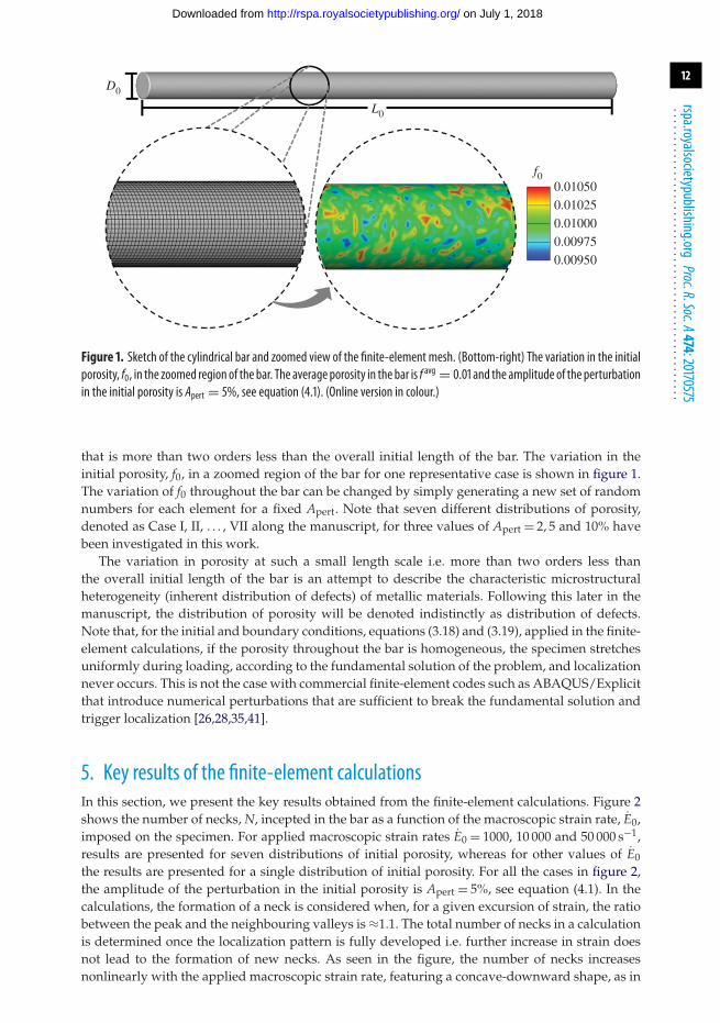
4. Three-dimensional finite-element modelThree-dimensional finite-element calculations are carried out to model the response of porouscylindrical bars subjected to initial and boundary conditions given in equations (3.18) and (3.19),respectively. The initial aspect ratio of the cylindrical bars analysed, figure 1, is, L0/D0 = 20, whereD0 = 2R0 = 2 mm is the initial cross-section diameter of the bar. The finite-element mesh of thecylindrical bar consists of 161 600 twenty-node brick elements with initial element dimensionsalong the axis of the bar being equal to L0/400. The three-dimensional finite-element calculationsare based on the dynamic principle of virtual work using a finite deformation Lagrangianconvected coordinate formulation, the constitutive framework detailed in §2, and the constitutiveparameters listed in table 1. A more detailed description of the finite-element formulation andimplementation of the same with additional references is given in [33,38–40].
Recall from the introduction that, in the classical statistical theories used to approach themultiple necking problem, distributions of material defects are assumed to be responsible for thedistributions of neck sizes in the localization pattern. In the calculations here, the initial porosityor the void volume fraction, f0, is randomly perturbed in the bar following,
f0 = f avg(1 + Apert × Rrand), (4.1)
where f avg = 〈f0〉 is the average initial void volume fraction, Apert is the amplitude of theperturbation and −1.0 ≤ Rrand ≤ 1.0 is a random number. The value of Rrand is generated for eachfinite-element in the bar, thus the porosity in the bar varies at the length scale of the finite-element
on July 1, 2018http://rspa.royalsocietypublishing.org/Downloaded from
12
rspa.royalsocietypublishing.orgProc.R.Soc.A474:20170575
...................................................
0.01050f0
L0
D0
0.009500.009750.010000.01025
Figure 1. Sketch of the cylindrical bar and zoomed view of the finite-element mesh. (Bottom-right) The variation in the initialporosity, f0, in the zoomed region of the bar. The average porosity in the bar is f avg = 0.01 and the amplitude of the perturbationin the initial porosity is Apert = 5%, see equation (4.1). (Online version in colour.)
that is more than two orders less than the overall initial length of the bar. The variation in theinitial porosity, f0, in a zoomed region of the bar for one representative case is shown in figure 1.The variation of f0 throughout the bar can be changed by simply generating a new set of randomnumbers for each element for a fixed Apert. Note that seven different distributions of porosity,denoted as Case I, II, . . . , VII along the manuscript, for three values of Apert = 2, 5 and 10% havebeen investigated in this work.
The variation in porosity at such a small length scale i.e. more than two orders less thanthe overall initial length of the bar is an attempt to describe the characteristic microstructuralheterogeneity (inherent distribution of defects) of metallic materials. Following this later in themanuscript, the distribution of porosity will be denoted indistinctly as distribution of defects.Note that, for the initial and boundary conditions, equations (3.18) and (3.19), applied in the finite-element calculations, if the porosity throughout the bar is homogeneous, the specimen stretchesuniformly during loading, according to the fundamental solution of the problem, and localizationnever occurs. This is not the case with commercial finite-element codes such as ABAQUS/Explicitthat introduce numerical perturbations that are sufficient to break the fundamental solution andtrigger localization [26,28,35,41].
5. Key results of the finite-element calculationsIn this section, we present the key results obtained from the finite-element calculations. Figure 2shows the number of necks, N, incepted in the bar as a function of the macroscopic strain rate, E0,imposed on the specimen. For applied macroscopic strain rates E0 = 1000, 10 000 and 50 000 s−1,results are presented for seven distributions of initial porosity, whereas for other values of E0the results are presented for a single distribution of initial porosity. For all the cases in figure 2,the amplitude of the perturbation in the initial porosity is Apert = 5%, see equation (4.1). In thecalculations, the formation of a neck is considered when, for a given excursion of strain, the ratiobetween the peak and the neighbouring valleys is ≈1.1. The total number of necks in a calculationis determined once the localization pattern is fully developed i.e. further increase in strain doesnot lead to the formation of new necks. As seen in the figure, the number of necks increasesnonlinearly with the applied macroscopic strain rate, featuring a concave-downward shape, as in
on July 1, 2018http://rspa.royalsocietypublishing.org/Downloaded from

13
rspa.royalsocietypublishing.orgProc.R.Soc.A474:20170575
...................................................
30
0 5 × 1041 × 104 2 × 10⁴ 3 × 10⁴ 4 × 10⁴
initial macroscopic strain rate, E·0 (s–1)
5
10
15
20
no. n
ecks
, N
25
fitted curve: N = 0.455(E·0)0.365
Figure 2. Finite-element results. Number of necks N versus applied macroscopic strain rate E0. For E0 = 1000, 10 000 and50 000 s−1 results are presented for seven distributions of initial porosity, whereas for other values of E0 results are presented fora single distribution of initial porosity. For all the cases, the amplitude of the perturbation in the initial porosity is Apert = 5%,see equation (4.1). The numerical results have been fitted with the curve N= 0.455(E0)0.365. (Online version in colour.)
1.4
0.8
0.9
1.0
1.1
1.2
1.3
norm
aliz
ed n
umbe
r of
nec
ks, N
/Nav
g
10%
average
I II III IVinitial porosity distribution
V VI VII
10%
E·0 = 1000 s–1
E·0 = 10 000 s–1
E·0 = 50 000 s–1
Figure 3. Finite-element results. Normalized number of necks N/Navg for three applied macroscopic strain rates E0 = 1000,10 000 and 50 000 s−1, and seven distributions of initial porosity. For all the cases, the amplitude of the perturbation in theinitial porosity is Apert = 5%, see equation (4.1). (Online version in colour.)
the experiments and numerical simulations reported for various ductile materials in [25,26,42–44].The numerical results have been fitted with the power law N = 0.455(E0)0.365.
The influence of the initial porosity distribution on the number of necks is further investigatedin figure 3 which shows the normalized number of necks N/Navg for seven distributions ofinitial porosity (denoted as I, II, . . . , VII) for three applied macroscopic strain rates (1000, 10 000and 50 000 s−1). Here, Navg is the average number of necks incepted in the bar considering theseven porosity distributions. For all the porosity distributions, the amplitude of the perturbationin the initial porosity is Apert = 5%, see equation (4.1). As seen in the figure, for E0 = 1000 s−1
there is a variation in the number of necks incepted, for example, N/Navg is 1.2 for the porositydistribution III and 0.85 for the porosity distribution VII. For E0 = 10 000 s−1, the variation in thenumber of necks for the various initial porosity distributions decreases and N/Navg lies withinthe range 0.9 ≤ N/Navg ≤ 1.1 for all seven distributions considered. At even higher loading rate,E0 = 50 000 s−1, the maximum variation in the N/Navg ratio is ≈ 5%. On the one hand, the factthat the number of necks in the bar increases with increasing applied strain rate contributes todecrease the variation of the N/Navg ratio with increasing E0. On the other hand, the results
on July 1, 2018http://rspa.royalsocietypublishing.org/Downloaded from

14
rspa.royalsocietypublishing.orgProc.R.Soc.A474:20170575
...................................................
7654321
180
0
30
60
90
150
120
10
0 7654normalized Lagrangian neck spacing, Lneck/D0 normalized Lagrangian neck spacing, Lneck/D0
normalized Lagrangian neck spacing, Lneck/D0
321 7654321
2
4
6
8
60
0
10
20
30
40
50no
. nec
ks, N
no. n
ecks
, N
E·0 = 1000 s–1
Case I
Case VIICase VICase VCase IVCase IIICase II
E·0 = 10 000 s–1
E·0 = 50 000 s–1
(a) (b)
(c)
Figure 4. Finite-element results. Histograms showing the number of necks N as a function of the normalized Lagrangian neckspacing Lneck/D0 for three applied macroscopic strain rates: (a) E0 = 1000 s−1, (b) E0 = 10 000 s−1 and (c) E0 = 50 000 s−1.The results corresponding to seven distributions of initial porosity (seven cases) are included in each histogram. The height of acoloured block within a bar of the histogram marks the number of necks with fixed Lneck/D0 for a given case. For all the cases,the amplitude of the perturbation in the initial porosity is Apert = 5%, see equation (4.1). For interpretation of the references tocolour in the text, the reader is referred to the web version of this article. (Online version in colour.)
in figure 3 also suggest that the increase in the applied strain rate reduces the influence of theporosity distribution (i.e. statistical variation in the material defect) on the number of necks thatdevelop in the bar. This can be attributed to the increasing role of inertia at high strain rates as in[26], which promotes the development of some specific wavelengths that play an important rolein controlling the neck spacing.
Next, histograms of number of necks, N, as a function of the normalized Lagrangian neckspacing, Lneck/D0, for the three applied strain rates investigated in figure 3 are presented infigure 4. The Lagrangian neck spacing, Lneck, is the distance between the central sections of twoconsecutive necks. For all the cases, the amplitude of the perturbation in the initial porosityis Apert = 5%. The results corresponding to seven distributions of initial porosity are includedin each histogram and each porosity distribution is plotted with a different colour (black, red,dark blue, etc.). As shown in figure 4a, for E0 = 1000 s−1 the distribution of neck spacings is veryheterogeneous and the normalized Lagrangian spacing varies in the range 1.9 ≤ Lneck/D0 ≤ 5.7,with an average value of 3.4. Hence, the neck spacings for E0 = 1000 s−1 are sensitive to the initialporosity distribution. For instance, for the porosity distribution III (dark blue) the neck spacingsvary from 1.9 to 3.7, while for the porosity distribution VI (light blue) they vary from 4.2 to 5.5. ForE0 = 10 000 s−1 (figure 4b), the distribution of neck spacings becomes less heterogeneous and thenormalized Lagrangian spacings vary from 0.8 to 2.3, with an average value of 1.7. Note that 68%of the neck spacings lie within the interval 1.5 ≤ Lneck/D0 ≤ 2. For E0 = 50 000 s−1 (figure 4c), thenormalized Lagrangian neck spacings vary from 0.4 to 1.1, with an average value of 0.8. Note that
on July 1, 2018http://rspa.royalsocietypublishing.org/Downloaded from

15
rspa.royalsocietypublishing.orgProc.R.Soc.A474:20170575
...................................................
t = 299 mst = 332 ms
2.5 1.8
0.6
0.8
1.0
1.2
1.4
1.6ra
tio b
etw
een
the
curr
ent a
ndth
e ba
ckgr
ound
cir
cum
fere
ntia
ltr
ue s
trai
n, E
qq/E
b qq
ratio
bet
wee
n th
e cu
rren
t and
the
back
grou
nd c
ircu
mfe
rent
ial
true
str
ain,
Eqq
/Eb qq
0.5
0.75
1.50
1.25
1.00
–0.50 0.500.25normalized axial coordinate, X
––0.25 0
1.0
1.5
2.0
–0.50 0.500.25normalized axial coordinate, X
––0.25 0
–0.50 0.500.25normalized axial coordinate, X
––0.25 0
t = 199 mst = 265 ms
Case V Case IVE·0 = 1000 s–1 E
·0 = 10 000 s–1
Case I
E·0 = 50 000 s–1
t = 53 mst = 60 ms
t = 66 mst = 73 ms
t = 40 mst = 26 mst = 33 ms
splits upinto 2 necks
splits upinto 2 necks
(a) (b)
(c)
Figure 5. Finite-element results. Time evolution of the ratio of the current and the background circumferential logarithmicstrain Eθθ /Ebθθ along the normalized axial coordinate X = X/L0 for three applied macroscopic strain rates: (a) E0 = 1000 s−1,(b) E0 = 10 000 s−1 and (c) E0 = 50 000 s−1. For all the cases, the amplitude of the perturbation in the initial porosity isApert =5%, see equation (4.1). (Online version in colour.)
the neck spacings are smaller than those obtained in the simulations presented in [26] for the samestrain rate using an ideal incompressible perfectly plastic material model. While the difference is,most likely, due to the plastic compressibility of the material considered in this paper, furtherresearch is still needed to clarify this point. Note that for E0 = 50 000 s−1, 88% of the neck spacingslie within a narrow interval of 0.75 ≤ Lneck/D0 ≤ 1. Hence, the distribution of neck spacings forE0 = 50 000 s−1 is nearly insensitive to the initial distribution of the porosity considered. In otherwords, at sufficiently high strain rates, the statistical variation in the material properties or defectsseems to have a smaller effect on the multiple necking patterns. The narrowing of the distributionof neck spacing and shifting to smaller lengths with increasing loading rate is in agreement withthe experimental observations of Zhang & Ravi-Chandar [12].
The fact that the increase in the applied strain rate reduces the influence of the statisticalvariation in the material defect on the number and pattern of necks that develop in the barseems to be reinforced by the results presented in figure 5. This graph shows the time evolution ofthe ratio of the current and the background circumferential logarithmic strain Eθθ /Eb
θθ along thenormalized axial coordinate X = X/L0 of the bar for the three applied strain rates investigatedin figures 3 and 4. The background strain, Eb
θθ = − 12 ln(A0/A), is the homogeneous strain,
equation (3.8).For E0 = 1000 s−1 (figure 5a), four different loading times are included in the graph to show
the onset and development of the necking pattern in the bar with the initial porosity distributionV. At t = 199 µs, which corresponds to an axial background strain E ≈ 0.18, equation (3.1), thecircumferential strain throughout the bar is very similar to the fundamental solution. At thispoint, the Considère strain (Econsidère = 0.08) has been exceeded, but the fluctuations in thecircumferential strain field are almost negligible and cannot be observed in the plot. As further
on July 1, 2018http://rspa.royalsocietypublishing.org/Downloaded from
16
rspa.royalsocietypublishing.orgProc.R.Soc.A474:20170575
...................................................
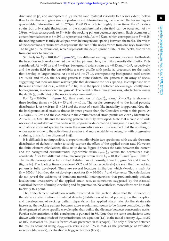
discussed in §6, and anticipated in §3, inertia (and material viscosity to a lesser extent) delaysflow localization and gives rise to a post-uniform deformation regime in which the bar undergoesquasi-stable deformation. At t = 265 µs, E ≈ 0.23 which is roughly three times the Considèrestrain, but only slight fluctuations in the circumferential strain field can be observed. At t =299 µs, which corresponds to E ≈ 0.26, the necking pattern becomes apparent. Each excursion ofcircumferential strain at t = 299 µs represents a neck. At t = 332 µs, which corresponds to E ≈ 0.28,the necking pattern is fully developed with heterogeneous spacing between the necks. The widthof the excursions of strain, which represents the size of the necks, varies from one neck to another.The height of the excursions, which represents the depth (growth rate) of the necks, also variesfrom one neck to another.
Similarly for E0 = 10 000 s−1 (figure 5b), four different loading times are considered to illustratethe inception and development of the necking pattern. Here, the initial porosity distribution IV isconsidered. At t = 53 µs and t = 60 µs, background axial strains are ≈0.43 and ≈0.47, respectively,and the strain field in the bar exhibits a wavy profile with peaks as precursors for the necksthat develop at larger strains. At t = 66 and t = 73 µs, corresponding background axial strainsare ≈0.51 and ≈0.55, the necking pattern is quite evident. The pattern is an array of necks,suggesting that there are finite wavelengths that determine the neck spacing. In comparison withthe results presented for E0 = 1000 s−1 in figure 5a, the spacing between necks is significantly morehomogeneous, as also shown in figure 4b. The height of the strain excursions, which characterizesthe depth (growth rate) of the necks, is also more uniform.
For E0 = 50 000 s−1 (figure 5c), time evolution of Eθθ /Ebθθ along X = X/L0 is shown at
three loading times: t = 26, t = 33 and t = 40 µs. The results correspond to the initial porositydistribution I. At t = 26 µs, E ≈ 0.84 and the onset of a neck-like instability is apparent. Note thatthe background axial strain is almost 10 times greater than the Considère strain at this point. Att = 33 µs, E ≈ 0.98 and the excursions in the circumferential strain profile are clearly identifiable.At t = 40 µs, E ≈ 1.10, and the necking pattern has fully developed. Note that a couple of widenecks split up into two narrow necks with progressive deformation giving rise to a regular patternwith almost constant spacing between the consecutive necks. It is assumed that the splitting ofwider necks is due to the activation of smaller and more unstable wavelengths with progressivestraining, this is further discussed in §6.
It is difficult, if not impossible, to experimentally obtain two specimens with exactly the samedistribution of defects in order to solely capture the effect of the applied strain rate. However,the finite-element calculations allow us to do so. Figure 6 shows the ratio between the currentand the background circumferential logarithmic strain Eθθ /Eb
θθ versus the normalized axialcoordinate X for two different initial macroscopic strain rates: E0 = 1000 s−1, and E0 = 10 000 s−1.The results correspond to two initial distributions of porosity, Case I (figure 6a) and Case VI(figure 6b). The loading times considered (332 and 66 µs, respectively) are such that the neckingpattern is fully developed. There are several locations in the bar which develop a neck forE0 = 1000 s−1 but they do not develop a neck for E0 = 10 000 s−1 and vice versa. The calculationsdo not reveal the existence of dominant material heterogeneities that predominantly activatelocalizations irrespective of the applied strain rate, as sometimes suggested by the classicalstatistical theories of multiple necking and fragmentation. Nevertheless, more efforts can be madeto clarify this point.
The finite-element calculation results presented in this section show that the influence ofthe statistical distribution of material defects (distribution of initial porosity) on the inceptionand development of necking pattern depends on the applied strain rate. As the strain rateincreases, the necking pattern becomes more regular, and seems to be (more) controlled by thedevelopment of some specific wavelengths that define the distance between consecutive necks.Further substantiation of this conclusion is pursued in §6. Note that the same conclusions weredrawn with the amplitude of the perturbation, see equation (4.1), in the initial porosity, Apert = 2%or 10%, instead of 5% (results for which are presented in this paper). The only difference betweenthe results obtained using Apert = 5% versus 2 or 10% is that, as the percentage of variationincreases (decreases), localization is triggered earlier (later).
on July 1, 2018http://rspa.royalsocietypublishing.org/Downloaded from

17
rspa.royalsocietypublishing.orgProc.R.Soc.A474:20170575
...................................................
–0.50
1.6
0.500.25normalized axial coordinate, X
––0.25 0 –0.50 0.500.25
normalized axial coordinate, X–
–0.25 0
ratio
bet
wee
n th
e cu
rren
t and
the
back
grou
nd c
ircu
mfe
rent
ial
true
str
ain,
Eqq
/Eb qq
0.6
0.8
1.0
1.2
1.4
Case I Case VI
0.6
2.0
1.8
1.6
1.4
1.2
1.0
0.8
E·0 = 1000 s–1
E·0 = 10 000 s–1
(a) (b)
Figure 6. Finite-element results. Variation in the ratio of the current and the background circumferential logarithmic strainEθθ /Ebθθ along the normalized axial coordinate X = X/L0 for two applied macroscopic strain rates: E0 = 1000 s−1 at theloading time t = 332µs, and E0 = 10 000 s−1 at the loading time t = 66µs. Two initial distributions of porosity (a) CaseI and (b) Case VI are considered. For all the cases, the amplitude of the perturbation in the initial porosity is Apert = 5%, seeequation (4.1). (Online version in colour.)
6. Comparison between linear stability analysis and finite-element resultsThe axial force F versus the macroscopic true strain averaged over the entire specimen Eavg, for thethree strain rates considered in figures 3–5, and three initial porosity distributions are comparedwith the fundamental solution, equation (3.20), in figure 7. The amplitude of the perturbationin the initial porosity for the finite-element calculations is Apert = 5% . As seen in figure 7, forall the applied strain rates, the force obtained from the finite-element calculations compareswell with the fundamental solution until the end of the post-critical regime. This suggests thatthe unloading waves emanating from the necks only influence the axial force after the post-critical regime (full localization). The notable oscillations in the axial force obtained from thefinite-element calculations in figure 7b,c around the maximum force are primarily due to thefact that the initial values of the field variables, equation (3.18), are not the exact fundamentalsolution of the problem. Therefore, the imposed velocity boundary conditions generate stresswaves resulting in the oscillations in the axial force. Nevertheless, these oscillations do not affectthe onset of the full localization because in our finite-element calculations necking does not occurin the absence of heterogeneous distribution of the initial porosity, §4. Also the oscillations vanishwithin the post-critical regime as seen in figure 7. The extent of the post-critical regime is stronglydependent on the applied strain rate but is unaffected by the initial distribution of the porosity. ForE0 = 1000 s−1, the post-critical regime ranges from the Considère strain (strain at maximum force)to the macroscopic strain level, E ≈ 0.26, at which the force decreases rapidly. For E0 = 10 000 s−1
and E0 = 50 000 s−1 the extent of the post-critical deformation regime is significantly greater,≈0.39 (figure 7b) and ≈ 0.90 (figure 7c), respectively. The current and the background strains arevirtually coincident in all sections of the bar during the post-critical regime (figure 5) because fulllocalization has not occurred yet.
Next, we compare the localization strain and average neck spacing obtained from the finite-element calculations and the predictions of the linear stability analysis. To this end, following[18,22,45], we introduce the concept of cumulative instability index defined as I = ∫t
tconsidère η+ dt,where tconsidère corresponds to the time at maximum force (onset of post-critical regime).Unlike the instantaneous perturbation growth η+, the cumulative index—which integrates thedimensional growth rate of the perturbation–tracks the history of the growth rate of all thegrowing modes during the post-critical deformation process and, as such, provides a moreaccurate description of the dominant necking modes which determine the localization patternfor each level of strain [22,35]. The reader is referred to the paper of Vaz-Romero et al. [35] tosee a comparison between the results obtained with the instantaneous perturbation growth and
on July 1, 2018http://rspa.royalsocietypublishing.org/Downloaded from

18
rspa.royalsocietypublishing.orgProc.R.Soc.A474:20170575
...................................................
maximum forceEavg = 0.08
0.4 0.80.70.60.50.40.30.2
2.0
1.51.20.90.60.3
0.10.3average macroscopic true strain, Eavg average macroscopic true strain, Eavg
average macroscopic true strain, Eavg
0.20.1
0
0.5
1.0
1.5
2.0ax
ial f
orce
, F (
kN)
axia
l for
ce, F
(kN
)0
0.5
1.0
1.5
2.0
0
0.5
1.0
1.5maximum force
Eavg = 0.08force dropEavg = 0.26
post-critical regime
E·0 = 50 000 s–1
E·0 = 1000 s–1 E
·0 = 10 000 s–1
post-critical regime
force dropEavg = 0.47
post-critical regime
maximum forceEavg = 0.08
force dropEavg = 0.98
fundamental solutionfinite elements: Case VIfinite elements: Case IVfinite elements: Case II
fundamental solutionfinite elements: Case VIfinite elements: Case IIfinite elements: Case I
fundamental solutionfinite elements: Case Vfinite elements: Case IIfinite elements: Case I
(a) (b)
(c)
Figure 7. Finite-element results. Axial force F versus average macroscopic true strain Eavg for three applied macroscopic strainrates: (a) E0 = 1000 s−1, (b) E0 = 10 000 s−1 and (c) E0 = 50 000 s−1. For each applied strain rate, finite-element results areshown for three initial distribution of porosity. The amplitude of the perturbation in the initial porosity is Apert = 5%, seeequation (4.1). The fundamental solution given by equation (3.20) is represented by the solid lines. (Online version in colour.)
the cumulative instability index for the problem of a nonlinear elastic bar subjected to dynamicstretching. The key point is the calibration of the cumulative index in such a manner that thepredictive capabilities of the stability analysis can be exploited. For this, we rely on the finite-element calculations corresponding to the lowest strain rate investigated E0 = 1000 s−1. Recallthat the linear stability analysis is only valid to describe the first stages of the necking patterndevelopment (as anticipated in §3). In other words, it is valid only when the neck-like deformationfield shows only a small deviation from the background strain (figure 5). In that case, the forceexerted on the bar is close to the fundamental solution (figure 7). The calculation for E0 = 1000 s−1
predicts that the drop of the force, i.e. the end of the post-critical regime and thus the upper boundof strain at which the stability analysis can be applied, occurs at t = 299 µs (which corresponds tomacroscopic axial strain E = 0.26). Inserting this value in the upper limit of the integral, whichdefines the cumulative index, we obtain I as a function of the normalized Lagrangian neckingwavelength Lneck/D0, calculated as Lneck/D0 = π/ξ (see [26]).
The I − Lneck/D0 curve for E = 0.26 is shown in figure 8a. Short wavelengths are dampeddue to stress multiaxiality effects and long wavelengths due to inertia, such that the curveI − Lneck/D0 shows a maximum for a given necking wavelength, called the critical neckingwavelength, denoted as (Lneck/D0)c. The corresponding value of the cumulative index, calledthe critical cumulative index, is denoted as Ic. For E0 = 1000 s−1 we have that (Lneck/D0)c = 3.89and Ic = 6.72. The critical wavelength determines the necking mode that grows the fastest anddefines the average neck spacing in the localization pattern. Next, we consider cases with appliedmacroscopic strain rates varying from 2500 to 50 000 s−1. This range of strain rates correspondsto values of the inertia parameter within the range 0.0126 ≤ H−1 ≤ 0.251. For each strain rate,
on July 1, 2018http://rspa.royalsocietypublishing.org/Downloaded from
19
rspa.royalsocietypublishing.orgProc.R.Soc.A474:20170575
...................................................
10
0
2
4
cum
ulat
ive
inst
abili
ty in
dex,
I
6
8
10
0
2
4
6
8
10
0
2
4
cum
ulat
ive
inst
abili
ty in
dex,
I
6
8
E·0 = 1000 s–1
E = 0.26
t = 299 msIc = 6.72
(L/D0)c = 3.98
Ic = 6.72
E·0 = 10 000 s–1
E = 0.43
t = 54 ms
(L/D0)c = 1.66
7654normalized Lagrangian necking wavelength, Lneck/D0
321 7654normalized Lagrangian necking wavelength, Lneck/D0
321
7654normalized Lagrangian necking wavelength, Lneck/D0
321
E·0 = 50 000 s–1
E = 0.89
t = 29 msIc = 6.72
(L/D0)c = 0.94
(a) (b)
(c)
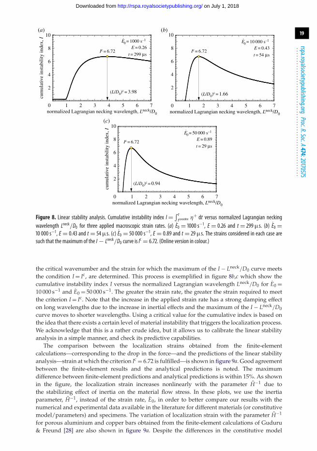
Figure 8. Linear stability analysis. Cumulative instability index I= ∫ttconsidère η
+ dt versus normalized Lagrangian neckingwavelength Lneck/D0 for three applied macroscopic strain rates. (a) E0 = 1000 s−1, E = 0.26 and t = 299µs. (b) E0 =10 000 s−1, E = 0.43 and t = 54µs. (c) E0 = 50 000 s−1, E = 0.89 and t = 29µs. The strains considered in each case aresuch that the maximum of the I − Lneck/D0 curve is Ic = 6.72. (Online version in colour.)
the critical wavenumber and the strain for which the maximum of the I − Lneck/D0 curve meetsthe condition I = Ic, are determined. This process is exemplified in figure 8b,c which show thecumulative instability index I versus the normalized Lagrangian wavelength Lneck/D0 for E0 =10 000 s−1 and E0 = 50 000 s−1. The greater the strain rate, the greater the strain required to meetthe criterion I = Ic. Note that the increase in the applied strain rate has a strong damping effecton long wavelengths due to the increase in inertial effects and the maximum of the I − Lneck/D0curve moves to shorter wavelengths. Using a critical value for the cumulative index is based onthe idea that there exists a certain level of material instability that triggers the localization process.We acknowledge that this is a rather crude idea, but it allows us to calibrate the linear stabilityanalysis in a simple manner, and check its predictive capabilities.
The comparison between the localization strains obtained from the finite-elementcalculations—corresponding to the drop in the force—and the predictions of the linear stabilityanalysis—strain at which the criterion Ic = 6.72 is fulfilled—is shown in figure 9a. Good agreementbetween the finite-element results and the analytical predictions is noted. The maximumdifference between finite-element predictions and analytical predictions is within 15%. As shownin the figure, the localization strain increases nonlinearly with the parameter H−1 due tothe stabilizing effect of inertia on the material flow stress. In these plots, we use the inertiaparameter, H−1, instead of the strain rate, E0, in order to better compare our results with thenumerical and experimental data available in the literature for different materials (or constitutivemodel/parameters) and specimens. The variation of localization strain with the parameter H−1
for porous aluminium and copper bars obtained from the finite-element calculations of Guduru& Freund [28] are also shown in figure 9a. Despite the differences in the constitutive model
on July 1, 2018http://rspa.royalsocietypublishing.org/Downloaded from

20
rspa.royalsocietypublishing.orgProc.R.Soc.A474:20170575
...................................................
finite elements–current worklinear stability–analysisfinite elements–aluminium. Guduru & Freund [28]
15%
15%
finite elements–current worklinear stability analysisfinite elements–aluminium. Guduru & Freund [28]finite elements–copper. Guduru & Freund [28]experiments–aluminium. Grady & Benson [46]experiments–copper. Grady & Benson [46]
finite elements–copper. Guduru & Freund [28]
1.4
0 0.300.250.200.150.100.05 0.300.25inertia parameter, H
– –1 inertia parameter, H– –1
0.200.150.100.05
0.2calibration data for the linear stability analysis
fitted curve: Eneck = 0.2145 + 1.8001 (H– –1)0.014678
fitted curve: Lneck /D0 = 0.57425(H– –1)–0.356
0.4
0.6
0.8
1.0
1.2
8
7
6
5
4
3
2
1
0
loca
lizat
ion
stra
in, E
neck
norm
aliz
ed L
agra
ngia
n ne
ck s
paci
ng,
Lne
ck/D
0
(a) (b)
Figure 9. Comparison between finite-element calculations performed here (current work), finite-element calculationsreported in Guduru & Freund [28], experiments reported in Grady & Benson [46] for aluminium and copper, and linear stabilityanalysis. In our finite-element calculations, the amplitude of the perturbation in the initial porosity is Apert = 5%, see equation(4.1). (a) Localization strain Eneck versus inertia parameter H−1. The linear stability results have been fitted with the curveEneck = 0.2145 + 1.8001(H−1)0.014678. (b) Average normalized Lagrangian neck spacing Lneck/D0 versus H−1. The linear stabilityresults have been fitted with the curve Lneck/D0 = 0.57425(H−1)−0.356. (Online version in colour.)
parameters used, and the fact that the numerical perturbations triggered localization in thecalculations of [28], a good qualitative agreement between their and our results is noted fromfigure 9a. The comparison between the average neck spacing obtained from the finite-elementcalculations and the critical wavelength predicted by the linear stability analysis—neckingwavelength for which the criterion Ic = 6.72 is fulfilled—is shown in figure 9b. The agreementbetween the numerical predictions and the analytical predictions is excellent. It shows that thelinear stability analysis, calibrated using a reference value for the cumulative index, can be usedto predict the average necks spacing in the bar for a wide range of values of H−1 (i.e. a wide rangeof applied strain rates). This is remarkable, especially taking into account the simplicity of theanalytical model which includes a series of hypotheses (wave effects neglected, one-dimensionalcharacter, linear nature, frozen perturbation coefficients, Bridgman correction, etc.) to make itmathematically tractable. In figure 9b, we also compare the variation of average neck spacing withH−1 for aluminium and copper bars obtained from the finite-element calculations of Guduru &Freund [28] and experiments of Grady & Benson [46] with our results. A good qualitativeagreement between our results and that of Guduru & Freund [28] is noted. In the experiments of[46], only a limited range of values of H−1 was covered, nevertheless, the experimental data showa decrease in Lneck/D0 with increasing H−1, in line with our results. The quantitative differencesin figure 9b is likely due to the differences in the constitutive model parameters considered hereand in [28], and the fact that the constitutive parameters used here were not calibrated to describethe mechanical response of the materials tested in [46].
Furthermore, the linear stability analysis allows us to explain the increasing (decreasing)scatter in the necks sizes obtained from the calculations as the applied strain rate decreases(increases) (figure 4). Figure 8 shows that the maximum of the I − Lneck/D0 curve becomes weaker(stronger) as the strain rate decreases (increases). In other words, the prevalence of the criticalnecking wavelength over the other wavelengths is weaker (stronger) as the strain rate decreases(increases). For the lower strain rates considered, the distribution of defects/porosities includedin the model can easily favour necking wavelengths different from the critical one that couldgrow faster, leading to the distribution of neck sizes reported in figure 4a. For the higher strainrates considered, the necking wavelengths close to the dominant one show a clear prevalence overother wavelengths, and the distributions of defects do not seem to promote the development ofany necking wavelength which is not near the critical one, as shown in figure 4c. These resultsshow that, as the strain rate increases, the spacing between necks in the localization patternbecomes more deterministic as they are more controlled by the inertial effects than the random
on July 1, 2018http://rspa.royalsocietypublishing.org/Downloaded from

21
rspa.royalsocietypublishing.orgProc.R.Soc.A474:20170575
...................................................
distribution of the material defects, (at least) for a given constitutive behaviour of the material.Recall that the linear stability results are obtained for strains for which, based on the finite-elementcalculations, the field variables in the bar remain close to the fundamental solution.
7. Summary and conclusionThis paper examines the inception and development of multiple necking patterns in porousmetallic bars subjected to dynamic tensile stretching at strain rates varying from 103 s−1 to0.5 × 105 s−1 using finite-element calculations and linear stability analysis. In the finite-elementcalculations, the initial porosity (representative of material defects) is varied randomly along thebar. The constitutive framework employed in the finite-element calculations includes many of thehardening and softening mechanisms that are characteristics of ductile metallic materials, suchas strain hardening, strain rate hardening, thermal softening and damage-induced softening. Thelinear stability analysis developed here, to the best of our knowledge, is the first of its kind forprogressively cavitating elastic-viscoplastic materials. The linear stability analysis also takes intoaccount the effects of inertia and stress multiaxiality. The key findings of this work are as follows:
— For the lower strain rates considered, the numerical results show that the distribution ofneck spacings is heterogeneous and is sensitive to the initial distribution of the porosity.In addition, different necks in the bar have markedly different sizes and growth rates. Arational explanation to these results stems from the linear stability analysis which showsthat, due to the limited contribution of inertia to the loading process, the critical neckingwavelength has a weak prevalence over other growing modes. This seems to be exploitedby the defect included in the calculations to favour necking wavelengths different fromthe critical one that could grow faster.
— For the higher strain rates considered, the numerical results show that the distributionof necks spacings is homogeneous and largely independent of the initial distribution ofthe porosity. In addition, different necks in the bar have similar growth rates and sizes.The linear stability analysis shows that, at high strain rates, with the increase in inertiaeffects, the critical necking wavelength has a strong prevalence over the other growingmodes. Hence, the heterogeneous distributions of the porosity do not promote neckingwavelengths which are not close to the critical one.
— The linear stability analysis, despite several simplifying assumptions, shows remarkablecapacity to predict the localization strain and the average neck spacings in the porousbar for the range of applied strain rates considered. To this end, the calibration of thelinear stability analysis using the cumulative instability index is the key, which wecarried out using the numerical results for the lowest applied strain rate. The qualitativeand quantitative agreement between linear stability analysis and finite-element resultssuggests that the analytical model captures many of the relevant mechanisms that controlthe emergence of the multiple necking patterns in the specimens.
In summary, the most important message of this paper is that the random distribution ofmaterial porosity triggers regular necking patterns at high strain rates. At high strain rates, inertiaeffects become important and the necking pattern seems not to be determined by the initialdistribution of the porosity. Here, we also show that at high applied strain rates, necking is notincepted at the maximum load (or Considère strain) but is followed by an extended post-criticalregime due to the stabilizing effects of inertia. The end of the post-critical regime corresponds tofull localization and at this point the load decreases rapidly. The extent of the post-critical regimeis found to increase with increasing applied strain rate. The extent of the post-critical regime isalso affected by the amplitude of the perturbation in the initial porosity. An increase (decrease)in the amplitude of the perturbation results in slight decrease (increase) in the extent of thepost-critical regime but does not affect significantly the necking pattern for a given distributionand loading rate. The post-critical regime will most likely be also affected by, the constitutive
on July 1, 2018http://rspa.royalsocietypublishing.org/Downloaded from

22
rspa.royalsocietypublishing.orgProc.R.Soc.A474:20170575
...................................................
behaviour of the material as suggested for fully dense materials in [19,20,26,47] and micro-inertiaeffects for porous materials [48–50]. The concerted numerical and analytical tool developed herecan now be used for future research needed to analyse the role of individual hardening/softeningmechanisms on the inception and development of multiple necking patterns in porous metallicbars subjected to dynamic tensile stretching. In addition, we note that with the advent of newadditive manufacturing techniques for metals, it will soon be possible to manufacture specimenswith controlled levels of porosity to fully validate our numerical and analytical results.
Data accessibility. This article has no additional data. All analytical and computational results are reproducible.Authors’ contributions. All authors contributed equally to this work.Competing interests. We declare we have no competing interests.Funding. K.E.N., S.O. and J.A.R.-M. acknowledge the support from the European Union’s Horizon2020Programme (Excellent Science, Marie-Sklodowska-Curie Actions) under REA grant agreement no. 675602(Project OUTCOME). J.A.R.-M. is also thankful to the Ministerio de Economía y Competitividad de España(Project no. EUIN2015-62556) for the financial support that partly supported this work.Acknowledgements. The authors acknowledge the fruitful discussions with Dr Guadalupe Vadillo (UniversityCarlos III of Madrid), Dr Alan Needleman (Texas A&M University, College Station), Dr Alain Molinari(University of Lorraine, Metz), Dr Sébastien Mercier (University of Lorraine, Metz) and Dr KrishnaswamyRavi-Chandar (University of Texas, Austin). The finite-element calculations reported on were carried outusing high performance research computing resources provided by Texas A&M University (http://www.hprc.tamu.edu).
References1. Mott NF, Linfoot EH. 1943 A theory of fragmentation. AC3348. London, UK: Ministry of Supply.2. Mott NF. 1943 Fragmentation of H. E. shells: a theoretical formula for the distribution of weights of
fragments. AC3642. London, UK: Ministry of Supply.3. Mott NF. 1943 A theory of the fragmentation of shells and bombs. AC4035. London, UK: Ministry
of Supply.4. Mott NF. 1943 Fragmentation of shell casings and the theory of rupture in metals. AC4613. London,
UK: Ministry of Supply.5. Mott NF. 1944 A theory of fragmentation. Application to wire wound bombs such as the American 20
lb. F. AC6338. London, UK: Ministry of Supply.6. Mott NF, Wilkinson JH, Wise TH. 1944 Fragmentation of service projectiles. AC6338. London,
UK: Ministry of Supply.7. Mott NF. 1947 Fragmentation of shell cases. Proc. R. Soc. A 189, 300–308. (doi:10.1098/
rspa.1947.0042)8. Grady D. 2006 Fragmentation of rings and shells the legacy of N. F. Mott, 1st edn. Berlin, Germany:
Springer.9. Grady DE, Kipp ME, Benson DA. 1984 Energy and statistical effects in the dynamic
fragmentation of metal rings. In Mechanical properties at high strain rates (ed. J Harding), pp.315–320. Bristol, UK: Institute of Physics.
10. Kipp ME, Grady DE. 1985 Dynamic fracture growth and interaction in one dimension. J. Mech.Phys. Solids 33, 399–415. (doi:10.1016/0022-5096(85)90036-5)
11. Grady D. 2002 Fragmentation of expanding cylinders and the statistical theory of N. F. Mott.In Shock compression of condensed matter - 2001 (eds MD Furnish, NN Thadhani, Y Horie), pp.799–802. College Park, MD: American Institute of Physics.
12. Zhang H, Ravi-Chandar K. 2006 On the dynamics of necking and fragmentation.I. Real-time and post-mortem observations in Al 6061-O. Int. J. Fract. 142, 183–217.(doi:10.1007/s10704-006-9024-7)
13. Zhang H, Ravi-Chandar K. 2008 On the dynamics of necking and fragmentation - II. Effectof material properties geometrical constraints and absolute size. Int. J. Fract. 150, 3–36.(doi:10.1007/s10704-008-9233-3)
14. Zhang H, Ravi-Chandar K. 2010 On the dynamics of localization and fragmentation. IV.Expansion of Al 6061-O tubes. Int. J. Fract. 163, 41–65. (doi:10.1007/s10704-009-9441-5)
15. Ravi-Chandar K, Triantafyllidis N. 2015 Dynamic stability of a bar under high loadingrate: response to local perturbations. Int. J. Solids Struct. 58, 301–308. (doi:10.1016/j.ijsolstr.2014.09.015)
on July 1, 2018http://rspa.royalsocietypublishing.org/Downloaded from
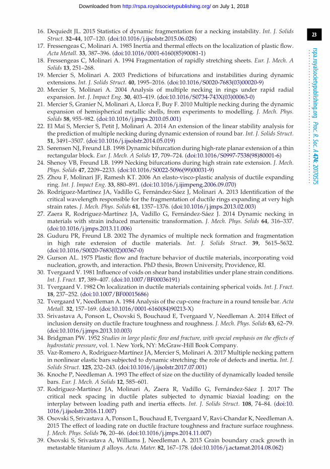
23
rspa.royalsocietypublishing.orgProc.R.Soc.A474:20170575
...................................................
16. Dequiedt JL. 2015 Statistics of dynamic fragmentation for a necking instability. Int. J. SolidsStruct. 32–44, 107–120. (doi:10.1016/j.ijsolstr.2015.06.028)
17. Fressengeas C, Molinari A. 1985 Inertia and thermal effects on the localization of plastic flow.Acta Metall. 33, 387–396. (doi:10.1016/0001-6160(85)90081-1)
18. Fressengeas C, Molinari A. 1994 Fragmentation of rapidly stretching sheets. Eur. J. Mech. ASolids 13, 251–268.
19. Mercier S, Molinari A. 2003 Predictions of bifurcations and instabilities during dynamicextensions. Int. J. Solids Struct. 40, 1995–2016. (doi:10.1016/S0020-7683(03)00020-9)
20. Mercier S, Molinari A. 2004 Analysis of multiple necking in rings under rapid radialexpansion. Int. J. Impact Eng. 30, 403–419. (doi:10.1016/S0734-743X(03)00063-0)
21. Mercier S, Granier N, Molinari A, Llorca F, Buy F. 2010 Multiple necking during the dynamicexpansion of hemispherical metallic shells, from experiments to modelling. J. Mech. Phys.Solids 58, 955–982. (doi:10.1016/j.jmps.2010.05.001)
22. El Maï S, Mercier S, Petit J, Molinari A. 2014 An extension of the linear stability analysis forthe prediction of multiple necking during dynamic extension of round bar. Int. J. Solids Struct.51, 3491–3507. (doi:10.1016/j.ijsolstr.2014.05.019)
23. Sørensen NJ, Freund LB. 1998 Dynamic bifurcation during high-rate planar extension of a thinrectangular block. Eur. J. Mech. A Solids 17, 709–724. (doi:10.1016/S0997-7538(98)80001-6)
24. Shenoy VB, Freund LB. 1999 Necking bifurcations during high strain rate extension. J. Mech.Phys. Solids 47, 2209–2233. (doi:10.1016/S0022-5096(99)00031-9)
25. Zhou F, Molinari JF, Ramesh KT. 2006 An elasto-visco-plastic analysis of ductile expandingring. Int. J. Impact Eng. 33, 880–891. (doi:10.1016/j.ijimpeng.2006.09.070)
26. Rodríguez-Martínez JA, Vadillo G, Fernández-Sáez J, Molinari A. 2013 Identification of thecritical wavelength responsible for the fragmentation of ductile rings expanding at very highstrain rates. J. Mech. Phys. Solids 61, 1357–1376. (doi:10.1016/j.jmps.2013.02.003)
27. Zaera R, Rodríguez-Martínez JA, Vadillo G, Fernández-Sáez J. 2014 Dynamic necking inmaterials with strain induced martensitic transformation. J. Mech. Phys. Solids 64, 316–337.(doi:10.1016/j.jmps.2013.11.006)
28. Guduru PR, Freund LB. 2002 The dynamics of multiple neck formation and fragmentationin high rate extension of ductile materials. Int. J. Solids Struct. 39, 5615–5632.(doi:10.1016/S0020-7683(02)00367-0)
29. Gurson AL. 1975 Plastic flow and fracture behavior of ductile materials, incorporating voidnucleation, growth, and interaction. PhD thesis, Brown University, Providence, RI.
30. Tvergaard V. 1981 Influence of voids on shear band instabilities under plane strain conditions.Int. J. Fract. 17, 389–407. (doi:10.1007/BF00036191)
31. Tvergaard V. 1982 On localization in ductile materials containing spherical voids. Int. J. Fract.18, 237–252. (doi:10.1007/BF00015686)
32. Tvergaard V, Needleman A. 1984 Analysis of the cup-cone fracture in a round tensile bar. ActaMetall. 32, 157–169. (doi:10.1016/0001-6160(84)90213-X)
33. Srivastava A, Ponson L, Osovski S, Bouchaud E, Tvergaard V, Needleman A. 2014 Effect ofinclusion density on ductile fracture toughness and roughness. J. Mech. Phys. Solids 63, 62–79.(doi:10.1016/j.jmps.2013.10.003)
34. Bridgman PW. 1952 Studies in large plastic flow and fracture, with special emphasis on the effects ofhydrostatic pressure, vol. 1. New York, NY: McGraw-Hill Book Company.
35. Vaz-Romero A, Rodríguez-Martínez JA, Mercier S, Molinari A. 2017 Multiple necking patternin nonlinear elastic bars subjected to dynamic stretching: the role of defects and inertia. Int. J.Solids Struct. 125, 232–243. (doi:10.1016/j.ijsolstr.2017.07.001)
36. Knoche P, Needleman A. 1993 The effect of size on the ductility of dynamically loaded tensilebars. Eur. J. Mech. A Solids 12, 585–601.
37. Rodríguez-Martínez JA, Molinari A, Zaera R, Vadillo G, Fernández-Sáez J. 2017 Thecritical neck spacing in ductile plates subjected to dynamic biaxial loading: on theinterplay between loading path and inertia effects. Int. J. Solids Struct. 108, 74–84. (doi:10.1016/j.ijsolstr.2016.11.007)
38. Osovski S, Srivastava A, Ponson L, Bouchaud E, Tvergaard V, Ravi-Chandar K, Needleman A.2015 The effect of loading rate on ductile fracture toughness and fracture surface roughness.J. Mech. Phys. Solids 76, 20–46. (doi:10.1016/j.jmps.2014.11.007)
39. Osovski S, Srivastava A, Williams J, Needleman A. 2015 Grain boundary crack growth inmetastable titanium β alloys. Acta. Mater. 82, 167–178. (doi:10.1016/j.actamat.2014.08.062)
on July 1, 2018http://rspa.royalsocietypublishing.org/Downloaded from

24
rspa.royalsocietypublishing.orgProc.R.Soc.A474:20170575
...................................................
40. Srivastava A, Osovski S, Needleman A. 2017 Engineering the crack path by controlling themicrostructure. J. Mech. Phys. Solids 100, 1–20. (doi:10.1016/j.jmps.2016.12.006)
41. Rusinek A, Zaera R. 2007 Finite element simulation of steel ring fragmentation under radialexpansion. Int. J. Impact Eng. 34, 799–822. (doi:10.1016/j.ijimpeng.2006.01.003)
42. Grady DE, Kipp ME. 1985 Mechanisms of dynamic fragmentation: factors governing fragmentsize. Mech. Mater. 4, 311–320. (doi:10.1016/0167-6636(85)90028-6)
43. Altynova M, Hu X, Daehn GS. 1996 Increased ductility in high velocity electromagnetic ringexpansion. Metall. Trans. A 27, 1837–1844. (doi:10.1007/BF02651933)
44. Grady DE, Olsen ML. 2003 A statistics and energy based theory of dynamic fragmentation.Int. J. Impact Eng. 29, 293–306. (doi:10.1016/j.ijimpeng.2003.09.026)
45. Petit J, Jeanclaude V, Fressengeas C. 2005 Breakup of copper shaped-charge jets:experiments, numerical simulations, and analytical modeling. J. Appl. Phys. 98, 123521.(doi:10.1063/1.2141647)
46. Grady DE, Benson DA. 1983 Fragmentation of metal rings by electromagnetic loading. Exp.Mech. 12, 393–400. (doi:10.1007/BF02330054)
47. Sørensen NJ, Freund LB. 2000 Unstable neck formation in a ductile ring subjected to impulsiveradial loading. Int. J. Solids Struct. 37, 2265–2283. (doi:10.1016/S0020-7683(98)00315-1)
48. Molinari A, Mercier S. 2001 Micromechanical modelling of porous materials under dynamicloading. J. Mech. Phys. Solids 49, 1497–1516. (doi:10.1016/S0022-5096(01)00003-5)
49. Sartori C, Mercier S, Jacques N, Molinari A. 2015 Constitutive behavior of porousductile materials accounting for micro-inertia and void shape. Mech. Mater. 80B, 324–339.(doi:10.1016/j.mechmat.2013.12.006)
50. Jacques N, Mercier S, Molinari A. 2015 A constitutive model for porous solids takinginto account microscale inertia and progressive void nucleation. Mech. Mater. 80B, 311–323.(doi:10.1016/j.mechmat.2014.01.008)
on July 1, 2018http://rspa.royalsocietypublishing.org/Downloaded from