Predicting porosity, permeability, and tortuosity of ... - Nature

1

Vol.:(0123456789)

Scientific Reports | (2020) 10:21488 | https://doi.org/10.1038/s41598-020-78415-x

www.nature.com/scientificreports

Predicting porosity, permeability, and tortuosity of porous media from images by deep learningKrzysztof M. Graczyk* & Maciej Matyka

Convolutional neural networks (CNN) are utilized to encode the relation between initial configurations of obstacles and three fundamental quantities in porous media: porosity ( ϕ ), permeability (k), and tortuosity (T). The two-dimensional systems with obstacles are considered. The fluid flow through a porous medium is simulated with the lattice Boltzmann method. The analysis has been performed for the systems with ϕ ∈ (0.37, 0.99) which covers five orders of magnitude a span for permeability k ∈ (0.78, 2.1× 10

5) and tortuosity T ∈ (1.03, 2.74) . It is shown that the CNNs can be used to predict the porosity, permeability, and tortuosity with good accuracy. With the usage of the CNN models, the relation between T and ϕ has been obtained and compared with the empirical estimate.

Transport in porous media is ubiquitous: from the neuro-active molecules moving in the brain extracellular space1,2, water percolating through granular soils3 to the mass transport in the porous electrodes of the Lithium-ion batteries4 used in hand-held electronics. The research in porous media concentrates on understanding the connections between two opposite scales: micro-world, which consists of voids and solids, and the macro-scale of porous objects. The macroscopic transport properties of these objects are of the key interest for various indus-tries, including healthcare5 and mining6.

Macroscopic properties of the porous medium rely on the microscopic structure of interconnected pore space. The shape and complexity of pores depend on the type of medium. Indeed, the pores can be elongated and interwoven showing a high porosity and anisotropy like in fibrous media7,8. On the other hand, the medium can be of low porosity with a tight network of twisted channels. For instance, in rocks and shales, as a result of erosion or cracks, large fissures can be intertwined in various ways6.

Porosity ( ϕ ), permeability (k), and tortuosity (T) are three parameters that play an important role in the description and understanding of the transport through the porous medium. The porosity is the fundamental number that describes the fraction of voids in the medium. The permeability defines the ability of the medium to transport fluid. Eventually, the tortuosity characterizes the paths of particles transported through the medium9,10. The porosity, permeability, and tortuosity are related by the Carman-Kozeny11 law, namely,

where S is the specific surface area of pores and c is the shape factor. The tortuosity is defined as the elongation of the flow paths in the pore space12,13:

where Leff is an effective path length of particles in pore space and L is a sample length ( L < Leff and thus, T > 1 ). The T is calculated from the velocity field obtained either experimentally or numerically. There are experimental techniques for particle path imaging in a porous medium, like particle image velocimetry14. However, they have limitations due to the types of the porous medium. There are two popular numerical approaches for estimation of T. In the first, the particle paths are generated by the integration of the equation of motion of fluid particles11,12. In the other, used in this work, T is calculated directly from the velocity field by averaging its components11,15. Indeed, the tortuosity is given by the expression

(1)k = ϕ3

cT2S2,

(2)T = Leff

L,

OPEN

Institute of Theoretical Physics, Faculty of Physics and Astronomy, University of Wrocław, pl. M. Borna 9, 50-204 Wrocław, Poland. *email: [email protected]

http://crossmark.crossref.org/dialog/?doi=10.1038/s41598-020-78415-x&domain=pdf

2

Vol:.(1234567890)


www.nature.com/scientificreports/

where 〈u〉 is the average of the magnitude of fluid velocity and 〈ux〉 is the average of its component along macro-scopic direction of the flow15. The pedagogical review of the approach is given by Matyka and Koza16, where the main features of the approach are explained in Figs. 3 and 5.

Calculating the flow in the real porous medium, with the complicated structure of pores, requires either a special procedure for grid generation in the standard Navier-Stokes solvers17 or usage of a kind of mesoscopic lattice gas-based methods18. Nevertheless of the type of solver used for the computation, the simulation procedure is time and computer resource consuming. Thus we propose the convolutional neural networks (CNN) based approach to simplify and speed up the process of computing the basic properties of a porous medium.

The deep learning (DL)19 is a part of the machine learning and artificial intelligence methods. It allows one to analyze or describe complex data. It is useful in optimizing the complicated numerical models. Eventually, it is a common practice to use the DL in problems not described analytically. The DL finds successful applications to real-life problems20 like automatic speech recognition, visual-image recognition, natural language processing, medical image analysis, and others. The DL has become an important tool in science as well.

Recently, the number of applications of the DL methods to problems in physics and material science grows exponentially21. One of the standard applications is to use the machine learning models to analyze the experi-mental data22. The deep neural networks are utilized to study the phase structure of the quantum and classical matters23. The DL is applied to solve the ordinary differential equations24–26. There are applications of the DL approaches to the problems of fluid dynamics. Here, the main idea is to obtain the relations between the system represented by the picture and the physical quantities, like velocities, pressure, etc.

The DL is one of the tools considered in the investigation of the transport in a porous medium. For instance, the neural networks are used to obtain porous material parameters from the wave propagation27. The perme-ability is evaluated using the multivariate structural regression28. It is obtained directly from the images29 too. The fluid flow field predictions by CNNs, based on the sphere packing input data, are given by Santos et al.30. The advantages of the usage of the machine learning techniques over physical models, in computing permeability of cemented sandstones, are shown by Male et al.31. The predictions of the tortuosity, for unsaturated flows in porous media, based on the scanning electron microscopy images, have been given by Zhang et al.32. Eventually, the diffusive transport properties have been investigated with CNNs, which take for the input the images of the media geometry only33.

Our goal is to find the dependence between the configurations of obstacles, represented by the picture, and the porosity, permeability, and tortuosity. The relation is going to be encoded by the convolutional neural network, which for the input takes the binary picture with obstacles and it gives, as an output, the vector (ϕ, k,T) . To auto-mate, simplify, and optimize the process we use the state of the art of CNNs and DL techniques combined with the geometry input and fluid solver based outputs. Namely, to train the networks, we consider a large number of synthetic, random, porous samples with controllable porosity. From various models and types of complex phenomena related to porous media flow like multi-phase18, multi-scale34, regular35, irregular7 or even granular36 media we chose the model of single-phase fluid flow through randomly deposited overlapping quads—the single-scale porous media model with controllable porosity. The training data set contains the porous media geometries with corresponding numerical values of the porosity, permeability, and tortuosity. The two latter variables are obtained from the flow simulations done with the lattice Boltzmann solver.

As a result of the analysis, we obtain two CNN models which predict the porosity, permeability, and tortuos-ity with good accuracy. The relative difference between the predictions and the ’true’ values, for our best model, does not exceed 6% . Eventually, we generate a blind set of geometry data for which we make predictions of the tortuosity and porosity. The obtained T(ϕ) dependence is in qualitative agreement with the empirical fits.

The paper is organized as follows: in “Lattice Boltzmann method” section the lattice Boltzmann method is introduced, “Deep learning approach” section describes the CNN approach and the method of the data genera-tion, whereas “Results and summary” section contains the discussion of the numerical results and summary.

Lattice Boltzmann methodThe data set consists of the rectangular pictures of the configuration of obstacles with corresponding quantities (labels): ϕ , k, and T, which are calculated from the lattice Boltzmann method (LBM) flow simulations.

The LBM has confirmed its capability to solve complex flows in complicated porous geometries37. It is based on the density distribution function, which is transported according to the discrete Boltzmann equation. In the single relaxation time approximation the transport equation reads:

where f (�r, t) is the density distribution function, �v is the macroscopic velocity, τ is the relaxation time and g is the Maxwell-Boltzmann distribution function at given velocity and density (see Duda et al.15 and He and Lu38).

The LBM solver provides information about the time evolution of the density function, which is used to evaluate the velocity field. We consider the pore-scale approach—the obstacles are completely solid, while the pores are completely permeable. Hence the velocity field is solved at the pore space. Each simulation starts with the zero velocity condition. The sample is exposed to an external gravity force that pushes the flow. Notice that we keep the number of iterations larger than 10,000 and less than 1,000,000. For the steady-state condition, we take the sum of the relative change of the velocity field in the pore space:

(3)T = �u��ux�

,

(4)∂f

∂t+ �v · ∇f = − 1

τ(f − g),

3

Vol.:(0123456789)



where u is the local velocity at the current time step (taken at nodes i,j), and u′ is the velocity at time step 500 times steps earlier. The local change of the velocity is monitored to verify if the steady-state is achieved. The exemplary velocity field resulting from the above procedure is shown in Fig. 1.

Deep learning approachConvolutional neural networks. The convolutional neural networks are used to code the information about the dependence between the initial configuration of obstacles, represented by the picture, and the porosity, tortuosity as well as permeability. The CNN is a type of deep neural network designed to analyze multi-channel pictures. It has been successfully applied for the classification39 and the non-linear regression problems40.

The CNN consists of a sequence of convolutional blocks and fully connected layers. In the simplest scenario, a single block contains a convolutional layer with several kernels. Usually, the pooling layer follows on the con-volutional layer, while in the hidden layer, the rectified linear units (ReLU)40 are considered, as the activation functions. The theoretical foundations of the convolutional networks are given by Goodfellow et al.41.

A kernel extracts a single feature of the input. The first layer of the CNN collects the simplest objects (features) such as edges, corners, etc. The next layers relate extracted features. The role of the pooling layer is to amplify the signal from the features as well as to reduce the size of the input. Usually, a sequence of fully connected layers follows on the section of the convolutional blocks.

The CNNs considered in this work contain the batch normalization layers42. This type of layer has been pro-posed to maintain the proper normalization of the inputs. It has been shown that having the batch normalization layers improves the network performance on the validation set. Moreover, it is a method of regularization, which is an alternative to the dropout technique43.

Data. We consider the random deposition model of a porous medium. It is the popular method for generat-ing porous structures for numerical solvers44,45. The samples are build of overlapping quad solids laying on the two-dimensional surface.

A total number of 100,000 one-channel figures with obstacles and predicted values of the porosity, tortuos-ity, and permeability have been prepared. A given figure, see Fig. 2, is the binary picture of the size 800× 400 . It includes two vertical margins of the width 200 (pixels) each. The margins are kept to reduce the influence of boundaries on the calculations of the porosity, tortuosity, and permeability. But, for the CNN analysis, they do

(5)c =∑

i,j

(ui,j − u′i,j)2

u2i,j,

Figure 1. The exemplary pore-scale velocity magnitude in the fluid flow calculated using the LBM based on configurations from Fig. 2—brighter the color larger velocity. Contrast and brightness are adjusted to visualize the structure of emerged flow paths.

Figure 2. Exemplary random porous samples at porosity ϕ = 0.95, 0.8 and 0.5 (from left to right), size 800× 400 . Black blocks represent obstacles for the flow, while the interconnected light gray area is the pore space filled by fluid. Black clusters, visible for ϕ = 0.5 , are the effect of the filling-gap algorithm used for prepossessing of the data, after generating with random deposition procedure. The gaps are not accessible for the fluid and, thus, we fill them before they are provided to the fluid solver and neural network.

4

Vol:.(1234567890)



not contain the information. Hence in the training and inference process, the picture without margins is taken as an input for the network. Effectively, the input has the size 400× 400.

Each figure consists of 400× 400 nodes, which are either free or blocked for the fluid flow. The periodic boundary condition is set at sides with margins, whereas two remaining sides are considered no-slip boundary condition. To generate the medium at given porosity, we start with an empty system and systematically add 4× 4 quad obstacles at random positions in the porous region. The margins are excluded from this deposition proce-dure. We do not consider blocking of sites, thus, obstacles may overlap freely. Each time an obstacle is placed, we update current porosity and stop, if the desired value is reached. In the next step of the generation of figures, we use the simple flood-filling algorithm to eliminate all the non-physical islands from each sample—Island is the pore volume completely immersed in solids. The exemplary porous samples, at three different porosity values, are shown in Fig. 2. Having the binary images of the pore space, the LBM solver calculates the velocity distribution from which the quantities of interest: the porosity, tortuosity, and permeability are obtained.

The success of the training of the network is determined by the quality of the data, its representative ability. The data should uniformly cover the space of label parameters. The ranges of the porosity, permeability, and tor-tuosity, for the systems discussed in our analysis, are given in Table 1. In the initial stage of the system generation procedure, the porosity of samples has been chosen from the uniform distribution. However, some of the samples have been not permeable. Therefore we notice the skewed character of the porosity distribution (see Fig. 3, left). As a consequence, the tortuosity distribution is skewed as well, with most of the systems at T < 1.5 . We found a few systems with T > 2.0 at low permeability, but they have been rejected from the final analysis because the predictions of the LBM solver are uncertain in this range. Moreover, to improve the learning process for higher porosity values, we generated additional samples with porosity ϕ > 0.85 . As a result, an important fraction of the samples belongs to the tail of the distributions. Training the network with such distributed data leads to the model with excellent performance on the data from the peak of distribution, and with the low predictive ability, for the systems from the tail of the distribution. We partially solve this problem by considering the re-weighted distribution of samples, namely,

• the data are binned in the two-dimensional histogram in the permeability and tortuosity;• for every bin we calculate the weight given by the ratio of the total number of samples to the number of

samples in a given bin;• the ratios form the re-weighted distribution of the samples;• during the training, labeled figures in the mini-batch, are sampled from the re-weighted distribution.

Table 1. The ranges of the porosity, permeability, and tortuosity obtained for the ensemble of 100,000 samples of the systems generated within the fluid flow simulation procedure.

Porosity Permeability Tortuosity

Min 0.37 0.78 1.03

Max 0.99 2.1× 105 2.74

Figure 3. The distribution of the generated samples (training and validation data sets together) with respect to porosity, permeability, and tortuosity.

5

Vol.:(0123456789)



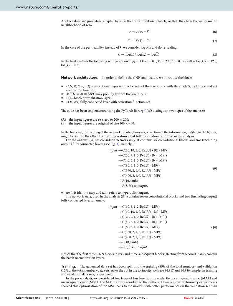
Another standard procedure, adapted by us, is the transformation of labels, so that, they have the values on the neighborhood of zero.

In the case of the permeability, instead of k, we consider log of k and do re-scaling:

In the final analyses the following settings are used: ϕs = 1.0 , ϕ = 0.5 , Ts = 2.8 , T = 0.5 as well as log(ks) = 12.3 , log(k) = 0.5 .

Network architecture. In order to define the CNN architecture we introduce the blocks:

• C(N, K, S, P, act) convolutional layer with: N kernels of the size K × K with the stride S, padding P and act - activation function;

• MP(K = 2) ≡ MP() max pooling layer of the size K × K;• B()—batch normalization layer;• F(M, act) fully connected layer with activation function act.

The code has been implemented using the PyTorch library47. We distinguish two types of the analyses:

(A) the input figures are re-sized to 200× 200;(B) the input figures are original of size 400× 400.

In the first case, the training of the network is faster, however, a fraction of the information, hidden in the figures, might be lost. In the other, the training is slower, but full information is utilized in the analysis.

For the analysis (A) we consider a network netA . It contains six convolutional blocks and two (including output) fully connected layers (see Fig. 4), namely:

where id is identity map and tanh refers to hyperbolic tangent.The network, netB , used in the analysis (B), contains seven convolutional blocks and two (including output)

fully connected layers, namely:

Notice that the first three CNN blocks in netA and three subsequent blocks (starting from second) in netB contain the batch normalization layers.

Training. The generated data set has been split into the training ( 85% of the total number) and validation ( 15% of the total number) data sets. After the cut in the tortuosity, we have 84,917 and 14,986 samples in training and validation data sets, respectively.

In the pre-analysis, we considered two types of loss functions, namely, the mean absolute error (MAE) and mean square error (MSE). The MAE is more sensitive to the outliers. However, our preliminary experiments showed that optimization of the MSE leads to the models with better performance on the validation set than

(6)ϕ →ϕ/ϕs − ϕ

(7)T →T/Ts − T .

(8)k → log(k)/ log(ks)− log(k).

(9)

input →C(10, 10, 1, 0, ReLU) · B() ·MP()

→C(20, 7, 1, 0, ReLU) · B() ·MP()

→C(40, 5, 1, 0, ReLU) · B() ·MP()

→C(80, 3, 1, 0, ReLU) ·MP()

→C(160, 2, 1, 0, ReLU) ·MP()

→C(400, 2, 1, 0, ReLU) ·MP()

→F(10, tanh)

→F(3, id) = output,

(10)

input →C(10, 5, 1, 2, ReLU) ·MP()

→C(10, 10, 1, 0, ReLU) · B() ·MP()

→C(20, 7, 1, 0, ReLU) · B() ·MP()

→C(40, 5, 1, 0, ReLU) · B() ·MP()

→C(80, 3, 1, 0, ReLU) ·MP()

→C(160, 2, 1, 0, ReLU) ·MP()

→C(400, 2, 1, 0, ReLU) ·MP()

→F(10, tanh)

→F(3, id) = output

6

Vol:.(1234567890)



the models optimized with the MAE. Therefore, the final analysis has been run with the MSE loss. During each epoch step, we calculate the error on the validation data set. The model with the smallest error value is saved.

The stochastic gradient descent (SGD) algorithm, in the mini-batch version, has been utilized for the training48,49. The mini-batch contains 250 (analysis (A)) and 65 (analysis (B)) samples, respectively. SGD is one of the simplest learning algorithms. But it is known that it regularizes naturally the networks. As a result, the obtained models work better on the validation data set20,50,51.

Results and summaryOne of the difficulties in the DL analyses is a proper choice of the hyperparameters, such as the size of the mini-batch, the optimization algorithm parameters, number of the CNN blocks, the size of the kernels, etc. We experimented with various configurations of the hyperparameters. Eventually, we established the final settings, namely, the SGD algorithm is run with the momentum 0.9 and the initial value of the learning rate 0.1. The lat-ter parameter is reduced by 10% every 50 epoch of the training. The sizes of the mini-batches as well as network architectures are reported in the previous section.

Both network architectures are constructed so that the number of filters in the CNN increases, while the size of the inputs of the subsequent layers reduces with the depth of the network. The kernels in the first layer of the netB are relatively large ( K = 10 ). In the subsequent layers, the kernels are smaller. The nB is the network netA with an additional input layer. In the case of the netA , instead of the layer with K = 10 , the input is re-sized. In both network schemes, (A) and (B), the output of the last CNN layer is a vector of the length 400.

The best model is the one with the smallest error on the validation set. Figs. 5 and 6 present the results for model netA , whereas Figs. 7 and 8 show the results for the analysis (B). In each figure, the predictions of the

Table 2. The mean of R and √Var(R) computed from the predictions of networks netA and netB. R is defined

by Eq. (11).

ϕ k T

netA

Training set

R − 5.27e−04 − 8.63e−04 − 1.65e−04

√Var(R) 9.40e−03 7.54e−02 2.47e−03

Validation set

R − 5.83e−04 − 8.88e−04 − 1.37e−04

√Var(R) 9.33e−03 5.55e−02 2.45e−03

netB

Training set

R − 2.64e−04 − 1.91e−04 2.81e−06

√Var(R) 7.44e−03 3.35e−02 2.01e−03

Validation set

Mean − 3.64e−04 − 1.48e−03 − 1.70e−05

√Var(R) 7.31e−03 6.28e−01 2.07e−03

Figure 4. The network netA architecture. It contains six convolutional blocks and two (including output) fully connected layers. Each convolutional block contains the max pooling layer. The first three convolutional blocks consist of the batch normalization layers. The graph was drawn using NN-SVG46.

7

Vol.:(0123456789)



porosity, permeability, and tortuosity versus the ‘true’ (as obtained from the LBM solver) values are plotted. Additionally, each figure contains the histograms of ratio

where R is computed for the porosity, permeability and tortuosity. More quantitative description of the histo-grams is given in Table 2, in which the mean ( R ) and variance

√Var(R) computed for all presented histograms

are given. The variable R is more informative than the standard metrics MSE or MAE, which give only qualitative information about goodness of fit. Notice that we present the network predictions for the training and valida-tion data sets.

The agreement between the network’s predictions and ‘true’ values seems to be pretty good. The performance of both networks is comparable. However, netA , with the resized input, seems to work better on the validation data set. Both models predict porosity well. The difficulties appeared in modeling the permeability and tortuosity.

(11)R = 1− predicted

true,

Figure 5. Predictions of the porosity, permeability, and tortuosity by the CNN versus ‘true‘ data (upper row). In the bottom row, the histograms of R, see Eq. (11), are plotted. The results are obtained for analysis (A) and the training data set. Solid line, in the top row, represents predicted = true equality.

Figure 6. Caption the same as in Fig. 5 but the predictions are made for the validation data set.

8

Vol:.(1234567890)



Indeed, it was difficult to obtain accurate model predictions for the low permeability and the tortuosity T > 1.75 . The re-weighting procedure described above, allowed to partially solve this problem. Another improvement is given by including the batch normalization layers in the network architecture.

In the analysis (A), for a large fraction of samples the relative difference between the network response and the ’true’ value is smaller than 6% . The most accurate predictions are obtained for the porosity and tortuosity. Indeed, the difference between ’true’ and predicted is smaller than 1% . Model netB computes the porosity and tortuosity with similar accuracy as the model netA , but the predictions of the permeability are rather uncertain in this case. The fact that the performance of both models is comparable shows that, in the case of porous media studied here, re-sizing of the input in the analysis (A) reduces only a small amount of information about the system. Moreover, model (A) has better performance on the validation data set than model (B). Hence, in our analysis, the re-sizing of the input figures works as a regularization of the model.

Both data sets, training, and validation are used in the optimization process. Hence to examine the quality of obtained models we generated the third set of the data. It contains 1, 300 unlabelled samples. This data set

Figure 7. Predictions of porosity, permeability, and tortuosity by CNN versus ‘true‘ data (upper row). In the bottom row, the histograms of R, see Eq. (11), are plotted. The results are obtained for analysis (B) and the training data set. Solid line, in the top row, represents predicted = true equality.

Figure 8. Caption the same as in Fig. 7 but the predictions are made for the validation data set.

9

Vol.:(0123456789)



is used to reconstruct the dependence between porosity and tortuosity, see Fig. 9). The obtained T(ϕ) relation agrees with the empirical fit from the analysis of the fluid flow12 on qualitative level. Indeed, tortuosity grows with ϕ → ϕc , where ϕc is the percolation threshold ( ϕ ≈ 0.4 for overlapping quads model52). Due to the finite size of the considered system, the actual percolation threshold is not sharp, and tortuosity around ϕc is underestimated in this area. The origin of the drop in the tortuosity below ϕc is the finite size of samples.

To summarize, we have shown that the convolutional neural network technique is a good method for pre-dicting the fundamental quantities of the porous media such as the porosity, permeability, and tortuosity. The predictions are made base on the analysis of the pictures representing the two-dimensional systems. The two types of networks have been discussed. In the first, the input pictures were resized, in the other, the input had the original size. We obtained good accuracy of predictions for all three quantities. The network models reproduce the empirical dependence between the tortuosity and porosity obtained in the previous studies12.

Received: 16 July 2020; Accepted: 17 November 2020

References 1. Rusakov, D. A. & Kullmann, D. M. Geometric and viscous components of the tortuosity of the extracellular space in the brain.

Proc. Natl. Acad. Sci. 95, 8975–8980 (1998). 2. Syková, E. & Nicholson, C. Diffusion in brain extracellular space. Physiol. Rev. 88, 1277–1340 (2008). 3. Nguyen, T. T. & Indraratna, B. The role of particle shape on the hydraulic conductivity of granular soils captured through Kozeny-

Carman approach. Géotechnique Lett. 10, 398–403 (2020). 4. Hossain, M. S. et al. Effective mass transport properties in lithium battery electrodes. ACS Appl. Energy Mater. 3, 440–446 (2019). 5. Suen, L., Guo, Y., Ho, S., Au-Yeung, C. & Lam, S. Comparing mask fit and usability of traditional and nanofibre n95 filtering

facepiece respirators before and after nursing procedures. J. Hosp. Infect. (2019). 6. Huaqing, X. et al. Effects of hydration on the microstructure and physical properties of shale. Petrol. Explor. Dev. 45, 1146–1153

(2018). 7. Koponen, A. et al. Permeability of three-dimensional random fiber webs. Phys. Rev. Lett. 80, 716 (1998). 8. Shou, D., Fan, J. & Ding, F. Hydraulic permeability of fibrous porous media. Int. J. Heat Mass Transf. 54, 4009–4018 (2011). 9. Backeberg, N. R. et al. Quantifying the anisotropy and tortuosity of permeable pathways in clay-rich mudstones using models

based on x-ray tomography. Sci. Rep. 7, 1–12 (2017). 10. Niya, S. R. & Selvadurai, A. A statistical correlation between permeability, porosity, tortuosity and conductance. Transp. Porous

Media 121, 741–752 (2018). 11. Koponen, A., Kataja, M. & Timonen, J. Permeability and effective porosity of porous media. Phys. Rev. E 56, 3319 (1997). 12. Matyka, M., Khalili, A. & Koza, Z. Tortuosity-porosity relation in porous media flow. Phys. Rev. E 78, 026306 (2008). 13. Ghanbarian, B., Hunt, A. G., Ewing, R. P. & Sahimi, M. Tortuosity in porous media: A critical review. Soil Sci. Soc. Am. J. 77,

1461–1477 (2013). 14. Morad, M. R. & Khalili, A. Transition layer thickness in a fluid-porous medium of multi-sized spherical beads. Exp. Fluids 46, 323

(2009). 15. Duda, A., Koza, Z. & Matyka, M. Hydraulic tortuosity in arbitrary porous media flow. Phys. Rev. E Stat. Nonlinear Soft Matter Phys.

84, 036319 (2011). 16. Matyka, M. & Koza, Z. How to calculate tortuosity easily? In AIP Conference Proceedings 4, Vol. 1453, 17–22 (American Institute

of Physics, 2012). 17. Boccardo, G., Crevacore, E., Passalacqua, A. & Icardi, M. Computational analysis of transport in three-dimensional heterogeneous

materials: an openfoamR©-based simulation framework. Comput. Vis. Sci. https ://doi.org/10.1007/s0079 1-020-00321 -6 (2020). 18. Bakhshian, S., Hosseini, S. A. & Shokri, N. Pore-scale characteristics of multiphase flow in heterogeneous porous media using the

lattice Boltzmann method. Sci. Rep. 9, 1–13 (2019). 19. LeCun, Y., Bengio, Y. & Hinton, G. Deep learning. Nature 521, 436EP (2015). 20. Rumelhart, D. E., Hinton, G. E. & Williams, R. J. Learning representations by back-propagating errors. Nature 323, 533–536. https

://doi.org/10.1038/32353 3a0 (1986).

Figure 9. Tortuosity versus porosity: solid line represents empirical relation T(ϕ) = 1− 0.77 log(ϕ) obtained within classical fluid flow approach12. The points are obtained from the unlabelled data set.

https://doi.org/10.1007/s00791-020-00321-6

https://doi.org/10.1038/323533a0

https://doi.org/10.1038/323533a0

10

Vol:.(1234567890)



21. Mehta, P. et al. A high-bias, low-variance introduction to machine learning for physicists. Phys. Rep. 810, 1–124. https ://doi.org/10.1016/j.physr ep.2019.03.001 (2019).

22. Graczyk, K. M. & Juszczak, C. Proton radius from Bayesian inference. Phys. Rev. C 90, 054334. https ://doi.org/10.1103/PhysR evC.90.05433 4 (2014) (1408.0150).

23. Carrasquilla, J. Machine Learning for Quantum Matter arXiv :2003.11040 (2020). 24. Lagaris, I., Likas, A. & Fotiadis, D. Artificial neural network methods in quantum mechanics. Comput. Phys. Commu. 104, 1–14.

https ://doi.org/10.1016/S0010 -4655(97)00054 -4 (1997). 25. Özbay, A. G., Laizet, S., Tzirakis, P., Rizos, G. & Schuller, B. Poisson CNN: Convolutional neural networks for the solution of the

Poisson equation with varying meshes and Dirichlet boundary conditions arXiv preprint arXiv :1910.08613 (2019). 26. Pannekoucke, O. & Fablet, R. Pde-netgen 1.0: from symbolic pde representations of physical processes to trainable neural network

representations. arXiv preprint arXiv :2002.01029 (2020). 27. Lähivaara, T., Kärkkäinen, L., Huttunen, J. M. & Hesthaven, J. S. Deep convolutional neural networks for estimating porous mate-

rial parameters with ultrasound tomography. J. Acoust. Soc. Am. 143, 1148–1158 (2018). 28. Andrew, M. Permeability prediction using multivariant structural regression. In E3S Web of Conferences, vol. 146, 04001 (EDP

Sciences, 2020). 29. Wu, J., Yin, X. & Xiao, H. Seeing permeability from images: fast prediction with convolutional neural networks. Sci. Bull. 63,

1215–1222 (2018). 30. Santos, J. E. et al. Poreflow-net: a 3d convolutional neural network to predict fluid flow through porous media. Adv. Water Resour.

138, 103539. https ://doi.org/10.1016/j.advwa tres.2020.10353 9 (2020). 31. Male, F., Jensen, J. L. & Lake, L. W. Comparison of permeability predictions on cemented sandstones with physics-based and

machine learning approaches. J. Nat. Gas Sci. Eng. 77, 103244 (2020). 32. Zhang, S., Tang, G., Wang, W., Li, Z. & Wang, B. Prediction and evolution of the hydraulic tortuosity for unsaturated flow in actual

porous media. Microporous Mesoporous Mater. 298, 110097 (2020). 33. Wu, H., Fang, W.-Z., Kang, Q., Tao, W.-Q. & Qiao, R. Predicting effective diffusivity of porous media from images by deep learning.

Sci. Rep. 9, 1–12 (2019). 34. Sabet, S., Mobedi, M. & Ozgumus, T. A pore scale study on fluid flow through two dimensional dual scale porous media with small

number of intraparticle pores. Polish J. Chem. Technol. 18, 80–92 (2016). 35. Ozgumus, T., Mobedi, M. & Ozkol, U. Determination of Kozeny constant based on porosity and pore to throat size ratio in porous

medium with rectangular rods. Eng. Appl. Comput. Fluid Mech. 8, 308–318 (2014). 36. Sobieski, W., Matyka, M., Gołembiewski, J. & Lipiński, S. The path tracking method as an alternative for tortuosity determination

in granular beds. Granular Matter 20, 72 (2018). 37. Succi, S. The Lattice Boltzmann Equation: For Fluid Dynamics and Beyond (Oxford University Press, Oxford, 2001). 38. He, X. & Luo, L.-S. Theory of the lattice Boltzmann method: From the Boltzmann equation to the lattice Boltzmann equation.

Phys. Rev. E 56, 6811 (1997). 39. Lecun, Y., Bottou, L., Bengio, Y. & Haffner, P. Gradient-based learning applied to document recognition. Proc. IEEE 86, 2278–2324

(1998). 40. Nair, V. & Hinton, G. E. Rectified linear units improve restricted boltzmann machines. In Proceedings of the 27th International

Conference on Machine Learning (ICML-10) (eds Fürnkranz, J. & Joachims, T.), 807–814 (2010). 41. Goodfellow, I., Bengio, Y. & Courville, A. Deep Learning (MIT Press, London, 2016). 42. Ioffe, S. & Szegedy, C. Batch normalization: Accelerating deep network training by reducing internal covariate shift arXiv preprint

arXiv :1502.03167 (2015). 43. Srivastava, N., Hinton, G., Krizhevsky, A., Sutskever, I. & Salakhutdinov, R. Dropout: A simple way to prevent neural networks

from overfitting. J. Mach. Learn. Res. 15, 1929–1958 (2014). 44. Chueh, C., Bertei, A., Pharoah, J. & Nicolella, C. Effective conductivity in random porous media with convex and non-convex

porosity. Int. J. Heat Mass Transf. 71, 183–188 (2014). 45. Li, Z., Galindo-Torres, S., Yan, G., Scheuermann, A. & Li, L. A lattice Boltzmann investigation of steady-state fluid distribution,

capillary pressure and relative permeability of a porous medium: Effects of fluid and geometrical properties. Adv. Water Resour. 116, 153–166 (2018).

46. LeNail, A. Nn-svg: Publication-ready neural network architecture schematics. J. Open Source Softw. 4, 747 (2019). 47. Paszke, A. et al. Pytorch: An imperative style, high-performance deep learning library. In Advances in Neural Information Processing

Systems 32, 8024–8035 (Curran Associates, Inc., 2019). 48. Bottou, L. Stochastic Gradient Descent Tricks 421–436 (Springer, Berlin, 2012). 49. Sutskever, I., Martens, J., Dahl, G. & Hinton, G. On the importance of initialization and momentum in deep learning. In Proceed-

ings of the 30th International Conference on Machine Learning, vol. 28 of Proceedings of Machine Learning Research (eds Dasgupta, S. & McAllester, D.) 1139–1147 (PMLR, Atlanta, 2013).

50. Bishop, C. M. Training with noise is equivalent to Tikhonov regularization. Neural Comput. 7, 108–116. https ://doi.org/10.1162/neco.1995.7.1.108 (1995).

51. Keskar, N. S., Mudigere, D., Nocedal, J., Smelyanskiy, M. & Tang, P. T. P. On large-batch training for deep learning: Generalization gap and sharp minima arXiv preprint arXiv :1609.04836 (2016).

52. Koza, Z., Matyka, M. & Khalili, A. Finite-size anisotropy in statistically uniform porous media. Phys. Rev. E Stat. Nonlinear Soft Matter Phys. 79, 066306 (2009).

AcknowledgementsThe publication was partially financed by the Initiative Excellence–Research University program for University of Wroclaw.

Author contributionsK.G. and M.M. conceived and conducted the project. K.G. designed and performed the deep learning analysis. M.M. designed and performed fluid flow simulations. K.G. and M.M. wrote and reviewed the manuscript.

Competing interests The authors declare no competing interests.

Additional informationCorrespondence and requests for materials should be addressed to K.M.G.

Reprints and permissions information is available at www.nature.com/reprints.

https://doi.org/10.1016/j.physrep.2019.03.001

https://doi.org/10.1016/j.physrep.2019.03.001

https://doi.org/10.1103/PhysRevC.90.054334

https://doi.org/10.1103/PhysRevC.90.054334

http://arxiv.org/abs/2003.11040

https://doi.org/10.1016/S0010-4655(97)00054-4



https://doi.org/10.1016/j.advwatres.2020.103539


https://doi.org/10.1162/neco.1995.7.1.108

https://doi.org/10.1162/neco.1995.7.1.108


www.nature.com/reprints

11

Vol.:(0123456789)



Publisher’s note Springer Nature remains neutral with regard to jurisdictional claims in published maps and institutional affiliations.

Open Access This article is licensed under a Creative Commons Attribution 4.0 International License, which permits use, sharing, adaptation, distribution and reproduction in any medium or

format, as long as you give appropriate credit to the original author(s) and the source, provide a link to the Creative Commons licence, and indicate if changes were made. The images or other third party material in this article are included in the article’s Creative Commons licence, unless indicated otherwise in a credit line to the material. If material is not included in the article’s Creative Commons licence and your intended use is not permitted by statutory regulation or exceeds the permitted use, you will need to obtain permission directly from the copyright holder. To view a copy of this licence, visit http://creat iveco mmons .org/licen ses/by/4.0/.

© The Author(s) 2020

http://creativecommons.org/licenses/by/4.0/

Predicting porosity, permeability, and tortuosity of ... - Nature

Documents

Transcript of Predicting porosity, permeability, and tortuosity of ... - Nature