Predicting Epileptic Seizures in Advance

Predicting Epileptic Seizures in AdvanceNegin Moghim*, David W. Corne

Heriot-Watt University, Edinburgh, United Kingdom

Abstract

Epilepsy is the second most common neurological disorder, affecting 0.6–0.8% of the world’s population. In thisneurological disorder, abnormal activity of the brain causes seizures, the nature of which tend to be sudden. AntiepilepticDrugs (AEDs) are used as long-term therapeutic solutions that control the condition. Of those treated with AEDs, 35%become resistant to medication. The unpredictable nature of seizures poses risks for the individual with epilepsy. It is clearlydesirable to find more effective ways of preventing seizures for such patients. The automatic detection of oncomingseizures, before their actual onset, can facilitate timely intervention and hence minimize these risks. In addition, advanceprediction of seizures can enrich our understanding of the epileptic brain. In this study, drawing on the body of work behindautomatic seizure detection and prediction from digitised Invasive Electroencephalography (EEG) data, a predictionalgorithm, ASPPR (Advance Seizure Prediction via Pre-ictal Relabeling), is described. ASPPR facilitates the learning ofpredictive models targeted at recognizing patterns in EEG activity that are in a specific time window in advance of a seizure.It then exploits advanced machine learning coupled with the design and selection of appropriate features from EEG signals.Results, from evaluating ASPPR independently on 21 different patients, suggest that seizures for many patients can bepredicted up to 20 minutes in advance of their onset. Compared to benchmark performance represented by a mean S1-Score (harmonic mean of Sensitivity and Specificity) of 90.6% for predicting seizure onset between 0 and 5 minutes inadvance, ASPPR achieves mean S1-Scores of: 96.30% for prediction between 1 and 6 minutes in advance, 96.13% forprediction between 8 and 13 minutes in advance, 94.5% for prediction between 14 and 19 minutes in advance, and 94.2%for prediction between 20 and 25 minutes in advance.

Citation: Moghim N, Corne DW (2014) Predicting Epileptic Seizures in Advance. PLoS ONE 9(6): e99334. doi:10.1371/journal.pone.0099334

Editor: Alice Y. W. Chang, Kaohsiung Chang Gung Memorial Hospital, Taiwan

Received November 12, 2013; Accepted May 14, 2014; Published June 9, 2014

Copyright: � 2014 Moghim, Corne. This is an open-access article distributed under the terms of the Creative Commons Attribution License, which permitsunrestricted use, distribution, and reproduction in any medium, provided the original author and source are credited.

Funding: This project was supported by a SICSA prize studentship (http://www.sicsa.ac.uk/) for the timespan of 09/2009-03/2013. This study was also part-supported by the Department of Computer Science, Heriot-Watt University (http://www.macs.hw.ac.uk/departments/computer-science.htm) for the timespan of09/2009 - 03/2013. The funders had no role in study design, data collection and analysis, decision to publish, or preparation of the manuscript.

Competing Interests: The authors have declared that no competing interests exist.

* E-mail: [email protected]

Introduction

Epilepsy is a neurological disorder, which affects 50 million

people worldwide. It can be managed in some patients using

prescription drugs. The remaining 20–30%, however, are likely to

have a relapse after the initial remission, and some may develop

drug resistant epilepsy [1]. Patients with uncontrolled epilepsy can

be affected by accidents caused by unforeseen seizures as well as

sudden unexpected death. They may also suffer from a multitude

of other unwanted side effects such as memory loss, depression and

other psychological disorders [2].

Despite the design of new anti-epileptic drugs, drug resistant

epilepsy still lacks an ultimate solution [1]. Resective surgery,

where the part of the brain that causes the seizures is removed [3],

can only be applied to a small fraction of drug-resistant patients,

the outcome of which is highly unpredictable. Additionally, the

cause of drug-resistance is unknown. Resistance to the traditional

AEDs in addition to the lack of effective seizure management

treatments for this large population of patients demands newer,

more effective seizure control therapies.

Electroencephalography (EEG) records electrical activity along

the scalp, via the placement on the scalp of multiple electrodes; it

measures voltage fluctuations resulting from ionic current flows

within the brain. The time series of such voltage fluctuations

(signals) recorded by the EEG is believed to correspond to neural

activity, and, by comparing and contrasting EEG records from

multiple patients, the EEG can therefore assist in discovering and

characterizing abnormal activity in the brain [4]. The EEG is a

very powerful diagnostic tool for many neurological disorders,

epilepsy in particular. It can be used to distinguish between

epileptic and non-epileptic seizures, via expert analysis of EEG to

find patterns corresponding to ‘inter-ictal epileptiform discharges’

that are prevalent in epileptic patients but rare otherwise [3]. EEG

can provide information about the location of the brain where the

abnormality is created, and also can be used for identifying the

type of epilepsy syndrome [4].

In most diagnostic and treatment-monitoring settings, the non-

invasive EEG is used in the form of a scalp EEG. This form of

EEG is however susceptible to low resolution of recordings and as

a result may miss out on underlying epileptic patterns. Invasive

EEG is used when non-invasive methods result in poor localisation

[5]. One setting in which an invasive EEG serves to be more

informative is pre-surgery evaluation for accurate localisation of

the seizure-focus [5].

With the wide use of digital EEG recording tools, these kinds of

data are becoming increasingly accessible for electronic manipu-

lation. While EEGs were formerly used as a diagnosis and

treatment specification tool for patients, access to the digitised

form of this information has helped generate new fields of

research, from neonatal seizure detection to understanding how

the seizure unfolds in the epileptic brain.

PLOS ONE | www.plosone.org 1 June 2014 | Volume 9 | Issue 6 | e99334

http://creativecommons.org/licenses/by/4.0/

http://crossmark.crossref.org/dialog/?doi=10.1371/journal.pone.0099334&domain=pdf

In recent years, there has been growing research interest in

seizure detection and prediction from EEG recordings. Being able

to predict seizures, and couple this information with state of the art

technology, will allow patients to take action prior to the

occurrence of the seizure, minimizing potential risk [4].

Prior to the occurrence of seizures, a number of clinical

symptoms have been shown to exist. These symptoms include

increases in oxygen availability, cerebral blood flow, blood-

oxygen-level-dependent signals, and changes in heart rate [6–9].

In addition to these changes, it is believed that an increased

number of critical interactions among the neurons in the focal

region unfold over time. This concept has allowed researchers to

study EEGs in an alternative way, in order to find correlates of

such processes and identify the pre-ictal (pre-seizure) state.

The main question researchers have been addressing is whether

characteristic features can be extracted from an EEG which

correlate with the occurrence (and time of the occurrence) of

seizures. In that case, treatments could move from therapeutic and

long-term preventive plans to on-demand strategies (i.e. immedi-

ately before the seizure occurs). In this context, Stein et al. [10]

have envisioned the use of fast-acting anticonvulsant substances,

while Fisher [11] has proposed deep-brain stimulation technology

in order to reset the brain as soon as seizure activity is detected, to

avoid the occurrence of seizures.

There is also the question of how a seizure occurs: is it a result of

a sudden transition, or a gradual change, in the dynamics of the

brain? The latter can be predicted through dynamics and is more

likely the case for focal epilepsies, whereas the former is impossible

to predict through dynamics and is more likely to be the case in

general epilepsy [12].

The first attempts at seizure detection and prediction were

carried out by Viglione and Walsh [13] in order to find seizure

precursors using linear approaches for absence seizure EEGs (an

‘absence seizure’ is a category of seizure associated with brief loss

of consciousness). Rogowski et al. [14] and later Salant et al. [15]

were able to find changes 6 seconds before seizure onset, using an

autoregressive model of the neuronal activity. Siegel et al. [16]

found changes among 1-minute epochs prior to the seizure, and

conducted further analysis on the spike occurrence rates in the

EEG, indicating decreased focal spike-rate along with an increased

rate of bilateral spikes before the seizure. This was followed by Le

Van Quyen et al. [17] who compared pre-seizure dynamic

variations to those of inter-ictal (between seizures) EEG and

discovered a dynamical similarity index which seemed to decrease

before seizures. Another groundbreaking discovery was made by

Iaesemidis et al. [18] using the Lyapunov exponent and an open

window analysis, revealing chaotic behaviour in invasive EEG and

a decrease in this behaviour before the seizure.

Litt et al. [19] conducted a controlled experiment on continuous

multi-day EEG recordings of a population of 5 patients evaluated

for epilepsy surgery. This study reported that quantitative signal

changes were detected 7 hours, 2 hours and 50 minutes prior to

the seizure onset, with an increase in accumulated energy 50

minutes prior to the seizure onset, suggesting that the cascade of

electrophysiological events, which have evolved from several hours

before the onset, can be identified as a reliable and timely

indication of seizures. The optimistic findings of this study were,

however, not reproducible in later studies [20]. Moreover, the

analytical approach used in this study did not lend itself to the

development of a potential automated prediction-based treatment.

Some other studies used an algorithmic approach on similar multi-

day EEG recordings. Iasemidis et al. [21] reported, on unseen test

data, Sensitivity 81% and Specificity 78%, for an average of 45.3

minutes in advance, on a dataset of only two patients. The method

used in Iademidis et al’s study is an algorithmic real-time statistical

method which continuously calculates only a single feature (the

short-term maximum Lyapunov exponent) and monitors T-index

curves of this measure, and produces an alarm, if and when the

measure exceeds a threshold. The same research group reported

(in Chaovalitwongse et al. [22]) a Sensitivity of 68% and a

Specificity of 85% for an average prediction window of 72 minutes

in advance of seizures, when the same algorithm was tested on a

population of 10 patients; the low Sensitivity of 68% had a large

standard deviation of 24.42%, indicating that the method

performed poorly on 20% of the patients The methods proposed

by these studies, when tested on a larger dataset, led to poor results

and were deemed unsuitable for real-life implementation.

Costa et al. [23] have tested various neural networks for

classifying EEG records into one of four classes: ictal, pre-ictal,

inter-ictal, and post-ictal. Ictal corresponds to the seizure activity,

pre-ictal corresponds to the 300 seconds leading up to the

occurrence of a seizure, post-ictal corresponds to the 300 seconds

immediately following a seizure, and inter-ictal to the period

between post-ictal and pre-ictal. They used 14 features for

classifying the EEG signals, based on signal energy attributes,

wavelet transforms and non-linear system dynamics. They carried

out their study on EEG recordings of two patients from the

Freiburg EEG Database [24].

Costa et al.’s study [23] reported Sensitivity 98.5%, Specificity

99.5% and Accuracy 98.5%; such high values in comparison with

previous work arguably highlight the value of feature engineering

and machine learning algorithms in individualised seizure

classification. However, this experiment was only run on a small

population of two patients, with limited independent repeats, and

insufficient detail to allow full replication, so the generalisability of

this level of performance in seizure classification is therefore still to

be assessed.

It is helpful to distinguish seizure detection studies from seizure

prediction studies. Seizure detection refers to the automatic

recognition of seizures shortly before or after the actual onset,

commonly in a short prediction window of a few seconds long.

Seizure prediction represents the automatic recognition of seizures

well in advance of the actual onset where the prediction window

can be several minutes long [1]. The distinction between the two is

important because their target application scenarios, and hence,

the potential treatment strategies facilitated, are likely to be

different. The results reported for detection are typically, and

understandably, higher than those reported for prediction; this is

simply because detecting an imminent seizure is easier than

predicting it several minutes in advance.

A related distinction can be made in terms of the focus of a

study. There are broadly two types: analysis-oriented, and

prediction-oriented. In analysis-oriented studies, the focus is on

analyzing the statistical properties of seizures. Typically, distinct

characteristics of the EEG are evaluated in a retrospective

manner, for their capability to discriminate between known ictal

(seizure) and non-ictal (non-seizure) states of the brain. These

studies are mainly aimed at exploratory analysis of the seizure

state, involving the quantification of various statistical and other

metrics of EEG that correlate with seizures [25,26]. In prediction-

oriented studies, the focus is on developing a predictive algorithm

that might be a candidate for intervention-based treatment. In

such studies, more attention is therefore paid to the use of features

that can be quickly computed from streaming EEG data, and to

the design of predictive algorithms [21,22,23]. The present study

draws from analysis-oriented studies with regard to choosing

features which are associated with good discrimination of the

seizure state, and follows other prediction-oriented studies in terms

Predicting Epileptic Seizures in Advance


of standards and protocols for method and evaluation. However,

the present work goes beyond other prediction-oriented studies in

terms of the coupling of a relatively long advance-prediction

window (20 to 25 minutes) with validation of our approach over a

relatively large sample (21 patients).

In this study, an advance prediction algorithm, ASPPR

(Advance Seizure Prediction via Pre-Ictal Relabeling), is described.

To use ASPPR for a specific patient, an initial data procurement

and annotation stage is necessary, whereby at least 24 hrs of EEG

data are recorded for that patient. A clinical expert then annotates

the data, and ASPPR is employed to learn predictive models from

that data; depending on the available computing hardware,

learning the predictive models may take 1 or 2 hours. The

resulting predictive models will be capable of operating in

microseconds, and can be used for real-time intervention on that

patient (provided it is installed on an appropriate device capturing

data from sensors worn by that patient). ASPPR learns several

distinct predictive models for a given patient, each associated with

a ‘time-in-advance’ parameter t, indicating that the model

attempts to predict that seizure onset will occur between t and

t+5 minutes from now. In this study, results are reported for the 21

models (from t = 0 to t = 20 minutes, in steps of 1 minute).

Independent applications of ASPPR are conducted on data from

each of 21 patients in the Freiburg EEG database [24]. Following

procurement of a patient’s data and the subsequent annotation of

‘ictal’ regions in the data by a suitable expert, the ASPPR method

comprises three main components: i) The feature selection

component, which selects 14 out of 204 features for each patient,

according to the ranking criteria of the ReliefF [27] feature

selection algorithm. (The reason for selecting 14 in this study is

given later in the ‘ReliefF’ subsection); ii) a simple data preparation

step is performed to generate a separate dataset for training each

specific ‘time-in-advance’ predictive model. iii) each individual

‘time-in-advance’ predictive model is trained, using a multi-class

Support Vector Machine (multi-class SVM) [28]; in the present

study, this training employs 10-fold cross validation on a randomly

identified 70% of the an individual patient’s data; the reported

results indicate performance on the remaining 30% not used in

training. Further, results for each individual patient are averaged

over ten independent repeats, each involving a different random-

ized 70%/30% split.

Results are reported regarding the performance of this

algorithm on each of the 21 patients represented in the Freiburg

EEG dataset [24], and contrasted with benchmark performance

measures obtained for each of the 21 patients by using Costa et al’s

[23] proposed 14 features to predict seizure onset (i.e. using

ASPPR for the t = 0 ‘time-in-advance’ model only, and omitting

the feature selection component). The ASPPR method consistently

outperforms the benchmark (which has an S1-Score – harmonic

mean of Sensitivity and Specificity - of 90.6% for predicting

seizure onset between 0 and 300 seconds in advance), and achieves

mean S1-Scores ranging from a minimum of 93.79% (for

prediction between 10 and 15 minutes in advance) to a maximum

of 96.30% (for prediction between 1 and 6 minutes in advance),

and above 94% for several other ‘time-in-advance’ regimes,

including: 96.13% for prediction between 8 and 13 minutes in

advance; and 94.2% for prediction between 20 and 25 minutes in

advance.

Materials and Methods

Source DatasetThe Freiburg EEG Database is one of the most cited resources

used in modern seizure detection and prediction experiments. It is

also one of the few publicly available invasive EEG datasets. The

database contains 24 hour-long continuous pre-surgical invasive

EEG recordings of 21 patients suffering from epilepsy, during

which time several seizures are triggered and recorded. The

patients vary widely in age, seizure type and seizure locality, but all

suffer from focal medically intractable epilepsy and were admitted

for pre-surgical evaluation at the Epilepsy Centre of the University

Hospital of Freiburg, Germany. The retrospective evaluation of

data received prior approval by the Ethics committee, Medical

Faculty, University of Freiburg. Informed consent was obtained

from each patient [24,29].

Prior to public release, the Freiburg team prepared the data as

follows. The data were recorded at a 256 Hz sampling rate, using

the Neurofile NT digital EEG over 128 channels. From these

electrodes, 6 channels were extracted by visual analysis of EEG

experts, 3 of which were in the epilepsy focal area of the brain.

The channels were labelled from 1–6, where channels 1–3

corresponded to focal recording and 4–6 comprised extra-focal

recordings. The locations of these channels varied for each patient.

Two types of signal files were prepared per patient: Ictal and Inter-

ictal. Each Ictal files contain an hour of EEG signals per patient.

There are typically three or four Ictal files per patient, each

representing a one-hour window straddling a single seizure event.

Hence, Ictal files hold ictal signals (corresponding to the seizure

itself, typically around 180 seconds) as well as pre-ictal (signals

from the 300 seconds immediately preceding a seizure), post-ictal

signals (from the 300 seconds immediately following an ictal

section) and inter-ictal signals (signals from all other time windows

– i.e. not within a seizure or within 300 seconds either before or

after a seizure).

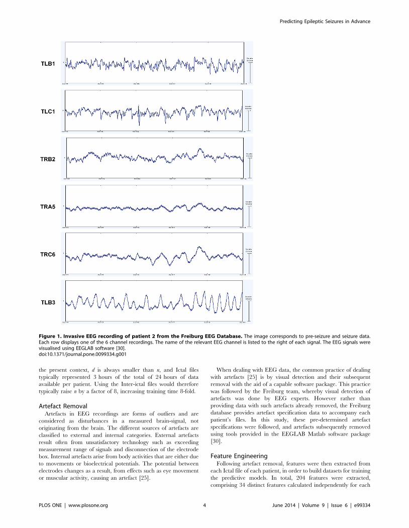
The data files are in ASCII format and contain the EEG time

series signals for 6 channels. The dataset comes with information

on electrode specifications of the 6 channels and seizure onset and

offset markers for all patients. Figure 1 displays EEG signals for

Patient 2 from the Freiburg EEG Database.

Data PreparationThis section clarifies how the Ictal files from the Freiburg

database were treated to produce datasets for use in the ASPPR

experiments. In short: (i) to reduce the time needed to build

predictive models, only Ictal files were used (omitting between 19

and 22 hours of data available per patient that contained only

EEG data further than 30 minutes from a seizure event); (ii)

artefacts in the data were handled precisely as described in the

notes accompanying the Freiburg database; (iii) a total of 204

feature time series were extracted for each patient (34 distinct

features for each of the 6 EEG channels), using EEGLAB [30]; (iv)

datasets were prepared comprising a time series of feature vectors

for each patient, with each data instance (at a given time point)

labeled appropriately as either ictal, pre-ictal, inter-ictal or post-ictal.

The final prepared datasets for all patients from the Freiburg

database can be accessed at https://code.google.com/p/asppr/.

Fuller detail on the data preparation steps are provided next.

Data SamplingIn the Freiburg EEG Database, both ‘Ictal’ and ‘Inter-ictal’ files

are provided. Only data from the time-periods represented by the

Ictal files were used. The Inter-ictal files only include non-seizure

data and hence may not contain traces of seizure activity. By using

only the data from the Ictal files, computational expense was

significantly reduced without omitting pre-ictal and ictal data. The

complexity of Support Vector Machine (SVM) learning is

O(max(n,d):min(n,d)2) [31], where n is the number of instances

in the training set and d is the number of features per instance. In



the present context, d is always smaller than n, and Ictal files

typically represented 3 hours of the total of 24 hours of data

available per patient. Using the Inter-ictal files would therefore

typically raise n by a factor of 8, increasing training time 8-fold.

Artefact RemovalArtefacts in EEG recordings are forms of outliers and are

considered as disturbances in a measured brain-signal, not

originating from the brain. The different sources of artefacts are

classified to external and internal categories. External artefacts

result often from unsatisfactory technology such as exceeding

measurement range of signals and disconnection of the electrode

box. Internal artefacts arise from body activities that are either due

to movements or bioelectrical potentials. The potential between

electrodes changes as a result, from effects such as eye movement

or muscular activity, causing an artefact [25].

When dealing with EEG data, the common practice of dealing

with artefacts [25] is by visual detection and their subsequent

removal with the aid of a capable software package. This practice

was followed by the Freiburg team, whereby visual detection of

artefacts was done by EEG experts. However rather than

providing data with such artefacts already removed, the Freiburg

database provides artefact specification data to accompany each

patient’s files. In this study, these pre-determined artefact

specifications were followed, and artefacts subsequently removed

using tools provided in the EEGLAB Matlab software package

[30].

Feature EngineeringFollowing artefact removal, features were then extracted from

each Ictal file of each patient, in order to build datasets for training

the predictive models. In total, 204 features were extracted,

comprising 34 distinct features calculated independently for each

Figure 1. Invasive EEG recording of patient 2 from the Freiburg EEG Database. The image corresponds to pre-seizure and seizure data.Each row displays one of the 6 channel recordings. The name of the relevant EEG channel is listed to the right of each signal. The EEG signals werevisualised using EEGLAB software [30].doi:10.1371/journal.pone.0099334.g001



of the 6 EEG channels. Extraction of a feature from an Ictal file

corresponded to generating a time series of feature values, where

the feature value at time t was calculated for each feature in the

way described below, from the signal values within a time window

ending at t. Following feature extraction, these 204 time series

were converted into a dataset by exporting the vector of feature

values for each time t starting from t = 5 seconds and continuing in

steps of 5 seconds until the end of the ictal file was reached. Hence,

for example, one hour of EEG data corresponded to 720 such data

instances, each with 204 features. The first 14 features, used only

for experiments to establish benchmark results, were drawn from

the feature-engineering approach taken by EPILAB [33,34] and

also by Costa et al. [23]. Additional features were then extracted

(an additional 20 features per channel) to support ASPPR’s

construction of more effective predictive models via feature

selection from a richer feature set.

The 14 features used in Costa et al. [23] are divided into three

general categories: signal energy, wavelet transform and non-

linear dynamics.

Features based on Signal EnergySignal energy and accumulated energy are commonly employed

features in EEG studies. A signal energy feature is typically the

mean of signal energy over a given period [35], which can be

expressed as in equation (1).

Energy(t,w)~1

w:Xi~t

i~t{w

s(i)2 ð1Þ

where s(i)denotes the signal’s amplitude at time-point i, and the

signal values are sampled in sequence starting at time-point 1 and

ending at time-point w.

Figure 2 displays the Signal Energy of patient 2 from the

Freiburg EEG Database, captured from all 6 channels. From

Figure 2, it can be observed that the signal energy produced by

each channel is particularly variable during the seizure.

Accumulated Energy (AE) is another powerful means of finding

abnormal behaviour in the brain, and commonly employed in

prediction-oriented seizure studies. AE in this article is the sum of

successive values of signal energy from a series of moving windows,

as expressed in equation (2),

AE(q)~1

100

Xt~q

t~1

Energy(t,w) ð2Þ

where AE(q) indicates the accumulated energy at time-point q,

calculated from successive values of signal energy via equation (1).

Figure 3 displays the changes in accumulated energy of patient 2,

calculated for each of the 6 EEG channels. The image displays

similar trends of accumulated energy through different seizure-

states for most channels. Channel 3 however displays a noticeably

different trend for both signal energy (as seen in Figure 2) and

accumulated energy. In potential intervention-based therapy, the

AE value would be regularly reset by the recording device in use,

most likely following a seizure episode, so that AE correlates with

the energy accumulated since the most recent seizure. Since AE

values are therefore not precisely known for the chronologically

first seizure of each patient in the Freiburg database (24% of the

seizures in the database), it is sensible to avoid bias by adding a

suitable random constant (a different constant per file) to the AE

values in each Ictal file (further details are provided with the

engineered dataset available at the link indicated above).

In this study, ‘Signal energy’ (also called ‘signal level’ in Costa et

al. [23]) was calculated for w = 1280, corresponding to 5 seconds at

the 256 Hz sampling rate of the raw data. Following Costa et al.

[23], two further signal energy features were also extracted,

corresponding to signal energy (equation (1)) averaged over

different windows. These were short-term energy (STE), where

w = 2304 (9 seconds), and long-term energy (LTE) where

w = 46080 (180 seconds).

Features based on Discrete Wavelet TransformsA Discrete Wavelet Transform (DWT) decomposes a signal, as

does a Fourier Transform, but in a way that is able to reflect both

frequency and temporal location properties of the signal, thereby

potentially capturing characteristics that may have been missed by

other features [36]. In particular, Fourier transforms are less able

to capture temporal localization properties. The DWT is done

with reference to a ‘mother wavelet’, which essentially controls the

fine detail of the composition. In feature extraction for EEG,

DWT is typically used to extract the signal energy component of a

specific frequency band over a specific time-window. Following

Costa et al. [23], we extracted eight features based on the DWT,

corresponding to the signal energy for four frequency bands at

each of two time windows. Once a component was extracted for a

specific frequency band, equation (1) was applied to this signal

component for a specific time window. The frequency bands

extracted were 0 Hz–12.5 Hz, 12.5 Hz–25 Hz, 25 Hz–50 Hz

and 50 Hz–100 Hz, and the time windows were ‘STE’, where

w = 2304 (9 seconds), and ‘LTE’, where w = 46080 (180 seconds).

The Daubechies mother wavelet [37] was used, with decompo-

sition level 4 using the EEGLAB tool [30].

Features based on non-linear dynamicsNon-linear features have had mixed review in the EEG signal-

processing community. In some studies they have been suggested

to be superior in performance in comparison to the linear features

due to the aperiodic and unpredictable behaviour of seizures

[17,18], while other studies suggest that linear attributes perform

as well, if not better than non-linear dynamics [25]. Non-linear

features are drawn from the theory of dynamical systems [38–40]

in contrast to the direct derivation of linear methods from the

time-series signal. Non-linear dynamical systems can represent

chaos, a perceivably unpredictable behaviour that is fundamen-

tally deterministic. Dynamical systems capture the behaviour of a

system in different states in time through fixed deterministic rules,

and the states at any given time are derived from a state space. In

this article, we used two features based on non-linear dynamics,

namely the maximum Lyapunov exponent and the correlation

dimension.

Lyapunov exponents [41,42] formally relates to the rate of

separation of infinitesimally, close trajectories in the phase space

(i.e. the space where all possible states of the system are

represented). Essentially they characterize the chaotic dynamics

of a system, and the ‘maximal Lyapunov exponent’ serves as a

surrogate measure for the stability of the system.

The correlation dimension [43] provides an alternative measure

related to stability; it is an estimate of the number of active degrees

of freedom of random points within a state space, and is calculated

using the correlation integral [44]. Extraction of both the maximal

Lyapunov exponent and the correlation dimension was done in

this work by using the corresponding functionality in TSTOOL (a

software package for analysing time-series data) [45], parameter-

ized to sample each of these in windows of length 1280 (5 seconds).



Additional Features: Moments, Spectral Band andSpectral Frequency

In addition to the 14 features above (used for recent prediction-

oriented seizure studies and consequently underpinning our

benchmark comparison), a further 20 distinct features were

extracted per EEG channel. The first 6 of these further 20

features comprised the standard statistical measures of mean,

skewness, and kurtosis of the raw signal value, averaged over STE

and LTE windows (9 seconds and 180 seconds respectively). These

represent the first, third and fourth standard statistical moments;

note that the existing ‘signal energy’ feature already captures

variance, which is the second moment.

A further ten features were extracted based on Spectral Band

Power (SBP). SBP is simply the signal energy in a specific

frequency range, as calculated via a Fourier transform. The ten

SBP features used in this study correspond to the ten combinations

arising from five frequency bands and the familiar two windows,

STE (9 seconds) and LTE (180 seconds). The five frequency bands

are chosen according to their common usage in analysis of

neuronal signals since they seem to capture useful information

[25], and are 0.5 Hz–4 Hz, 4 Hz–8 Hz, 8 Hz–13 Hz, 13 Hz–

30 Hz, and 30 Hz–48 Hz; these bands are respectively termed a,

b, c, d, and e. SBP feature extraction was implemented using SBP

functions In EEGLAB [30].

Finally, four features were extracted relating to Spectral Edge

Frequency (SEF) [32]. SEF is a measure that characterises the

signal’s energy distribution in terms of how signal power is

concentrated in the frequency spectrum. The measure SEF-X

measure indicates the lowest frequency F such that X% of the

spectral power is contained within the frequency band 0.5 Hz–F

Hz. In this paper we use four features that comprise SEF-90 and

SEF-50 (also called the median frequency), each measured over

both the 9-seconds STE and 180-seconds LTE windows, and

implemented using SEF functions available in EEGLAB [30].

Labeling of Data InstancesFollowing the feature extraction phase, each data instance

(recall: a data instance is a vector of features associated with a

specific time-point) was labeled as one of the following states:

Ictal. This labels the seizure activity in the brain and is marked

precisely by EEG experts. It is of varying length but is typically

close to 3 minutes long.

pre-ictal. pre-ictal is marked as the 5 minutes immediately prior

to the seizure onset and is believed to hold predictive markers of

seizure activity [46,47].

post-ictal. post-ictal is marked as brain activity following the

seizure offset for a duration of 5 minutes. Abnormal excitement in

the signals may be observed in this state, particularly as patients

are recovering from the seizures.

Figure 2. Signal Energy over 6 EEG channels for patient 2 from the Freiburg EEG Database. There is ictal activity from seconds 5 through35. SE stands for Signal Energy.doi:10.1371/journal.pone.0099334.g002



inter-ictal. non-seizure data preceding the pre-ictal state and

proceeding the post-ictal state are marked as inter-ictal, where

studies have traced early predictors of future seizure activity [48–

50].

Figure 4 further illustrates the signal divisions of the EEG signals

of a patient from the Freiburg EEG database. These labels were

manually set according to the seizure onset and end markers

provided in the Freiburg EEG Database notes. In training the

predictive models, we use 4 states rather than 2 states as practiced

in [23], since intuition suggests that distinguishing the activity

among the four states will benefit the learning process, and

facilitate a more even balance that avoids dominance of the inter-

ictal states over ictal activity. When reporting test set results,

however, these are always calculated on a 2-state basis (the

‘positive’ state being associated with a specific time-period in

advance of a seizure).

Finally, the data labeling step described here was used to

produce the dataset for training the ‘t = 0’ predictive models – in

other words, models that attempt to distinguish pre-ictal instances

from others, where a pre-ictal instance corresponds precisely to the

expectation that seizure onset will occur between 0 and 5 minutes

in the future. To produce training data for the ‘t = N’ predictive

models, where N ranged from 1 minute to 20 minutes in steps of 1

minute, specific and simple manipulation was applied to the ‘t = 0’

dataset, which is detailed later.

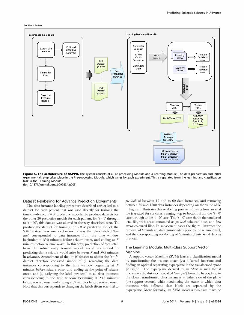
Advance Prediction Experiments: ASPPRIn total, 441 ‘advance prediction’ experiments are summarized

in this article. Following a feature selection stage for each

individual patient (see Figure 5), these experiments comprise the

training and evaluation of 21 distinct ‘time-in-advance’ predictive

models (from ‘t = 0’ to ‘t = 20’) for each of the 21 distinct patients

represented in the Freiburg EEG database. Each of these

experiments comprised ten independent trials, each of which

was identical except for a different random split of the data into a

training-set (70% of the instances) and a test set (30% of the

instances). Experiments were parallelised over a cluster of thirty 8-

core 64bit CentOS machines using Matlab parallel pooling [51].

ReliefFReliefF [27] is a feature estimator algorithm, used for feature

selection within ASPPR. ReliefF is a multi-class version of the

original and well-known Relief algorithm [52]. ReliefF starts by

assigning a weight of zero to each feature, and then works by

iterating the following: a random data instance is sampled, and a

sample of the closest data instances from the same class, and the

closest data instances from other classes, are found. Calculations

Figure 3. Accumulated Energy over 6 EEG channels for patient 2 from the Freiburg EEG Database. There is ictal activity from seconds 5through 35. AE stands for Accumulated Energy.doi:10.1371/journal.pone.0099334.g003



are then applied to adjust the feature weights, serving to enhance

the relative weights of features that seem more important for

discrimination between classes. A clear description of the ReliefF

algorithm may be found in Robnik-Sikonja and Kononenko [53].

The output of ReliefF is a vector of feature weights, which is then

used straightforwardly to rank the features in order of importance.

ReliefF is stochastic, and therefore every time feature ranking is

performed it is repeated ten times independently, and the overall

feature ranking is based on the mean weights emerging from these

ten trials. The computational complexity of ReliefF is suitable for

large datasets, being O(n6f ) [53], where n is the number of data

instances and f is the number of features.

For each patient, prior to building the predictive models for that

patient, ReliefF is used to find the 14 highest-ranked from the total

of 204 extracted features; this set of 14 features is taken forward

into the Learning module (Figure 5). The extraction of feature-sets

of size 14 was done to facilitate comparison with benchmark

results, which use a specific 14-feature subset from a previous

study. In this way, better (or worse) performance can clearly be

attributed to the choice of features themselves, rather than a

function of the size of the feature set. However, without this

constraint, optimized feature sets for different patients may well be

of varying size; this is a topic for future work.

It was found that this set of 14 features varied both within and

between patients; that is, for an individual patient, the top-14

features tended to vary across the ten independent trials of the

feature selection stage. Similarly, feature-sets would typically be

different for different patients. These observations are further

discussed later in this article.

Figure 4. An annotated epoch of the Invasive EEG of an epileptic seizure. All four states of ictal, pre-ictal, ictal, post-ictal and inter-ictal arecolour coded. EEG signals belong to patient 2 from the Freiburg EEG Database and were visualised using the EEGLAB software [30].doi:10.1371/journal.pone.0099334.g004



Dataset Relabeling for Advance Prediction ExperimentsThe data instance labeling procedure described earlier led to a

dataset for each patient that was used directly for training the

time-in-advance ‘t = 0’ predictive models. To produce datasets for

the other 20 predictive models for each patient, for ‘t = 1’ through

to ‘t = 20’, this dataset was altered in the way described next. To

produce the dataset for training the ‘t = N’ predictive model, the

‘t = 0’ dataset was amended in such a way that data labeled ‘pre-

ictal’ corresponded to data instances from the time window

beginning at N+5 minutes before seizure onset, and ending at N

minutes before seizure onset. In this way, prediction of ‘pre-ictal’

from the subsequently trained model would correspond to

predicting that a seizure would arise between N and N+5 minutes

in advance. Amendment of the ‘t = 0’ dataset to obtain the ‘t = N’

dataset therefore consisted simply of (i) removing the data

instances corresponding to the time window beginning at N

minutes before seizure onset and ending at the point of seizure

onset, and (ii) assigning the label ‘pre-ictal’ to all data instances

corresponding to the time window beginning at N+5 minutes

before seizure onset and ending at N minutes before seizure onset.

Note that this corresponds to changing the labels (from inter-ictal to

pre-ictal) of between 12 and to 60 data instances, and removing

between 60 and 1200 data instances depending on the value of N.

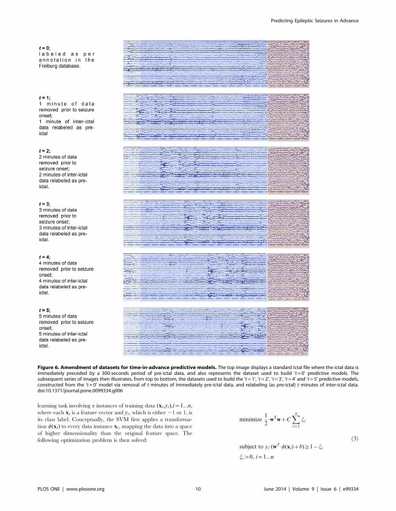
Figure 6 illustrates this relabeling process, showing how an ictal

file is treated for six cases, ranging, top to bottom, from the ’t = 0’

case through to the ‘t = 5’ case. The ‘t = 0’ case shows the unaltered

ictal file, with areas annotated as pre-ictal coloured blue, and ictal

areas coloured lilac. In subsequent cases the figure illustrates the

removal of t minutes of data immediately prior to the seizure onset,

and the corresponding re-labeling of t minutes of inter-ictal data as

pre-ictal.

The Learning Module: Multi-Class Support VectorMachine

A support vector Machine (SVM) learns a classification model

by transforming the instance-space (via a kernel function) and

finding an optimal separating hyperplane in the transformed space

[28,54,55]. The hyperplane derived by an SVM is such that it

maximizes the distance (so-called ‘margin’) from the hyperplane to

the closest transformed data instances at either side of the plane

(the support vectors), while maximizing the extent to which data

instances with different class labels are separated by the

hyperplane. More formally, an SVM solves a two-class machine

Figure 5. The architecture of ASPPR. The system consists of a Pre-processing Module and a Learning Module. The data preparation and initialexperimental setup takes place in the Pre-processing Module, which varies for each experiment. This is separated from the learning and classificationtask in the Learning Module.doi:10.1371/journal.pone.0099334.g005



learning task involving n instances of training data (xi,yi),i~1:::n,

where each xi is a feature vector and yi, which is either 21 or 1, is

its class label. Conceptually, the SVM first applies a transforma-

tion w(xi) to every data instance xi, mapping the data into a space

of higher dimensionality than the original feature space. The

following optimization problem is then solved:

minimize1

2:wTwzC

Xn

i~1

ji

subject to yi:(wT :w(xi)zb)§1{ji

jiw0, i~1:::n

ð3Þ

Figure 6. Amendment of datasets for time-in-advance predictive models. The top image displays a standard Ictal file where the ictal data isimmediately preceded by a 300-seconds period of pre-ictal data, and also represents the dataset used to build ‘t = 0’ predictive models. Thesubsequent series of images then illustrates, from top to bottom, the datasets used to build the ‘t = 1’, ‘t = 2’, ‘t = 3’, ‘t = 4’ and ‘t = 5’ predictive models,constructed from the ‘t = 0’ model via removal of t minutes of immediately pre-ictal data, and relabeling (as pre-ictal) t minutes of inter-ictal data.doi:10.1371/journal.pone.0099334.g006



where w is weight vector in the transformed space, b is a scalar (the

equation wT :w(x)zb~0 defines the desired hyperplane), C is a

regularisation parameter, and the ji,are non-negative ‘slack

variables’. Without the slack variables (equivalently, with all the

slack variables set at zero), the SVM is termed ‘hard-margin’, and

the constraint in equation (3) forces all instances with label 1 to be

mapped to one side of the hyperplane, and all instances with label

21 to be mapped to the other side. With slack variables allowed to

be nonzero, the SVM is denoted ‘soft-margin’, and the formula-

tion can cope with misclassifications (that is, the constraint can be

satisfied for some collection of ji, values). Minimization of the

upper expression in equation (3) promotes generalization perfor-

mance by keeping weight values low, and also minimizes the

degree to which misclassified instances are on the wrong side of the

hyperplane. The transformation w(xi)is ‘conceptual’ in the sense

that it is never directly applied. Instead, a kernel function K is used,

such that:

K(xi,xj)~w(xi)Tw(xj) ð4Þ

By using the kernel function directly, and exploiting the fact that

the optimization process only requires the calculation of dot-

products between transformed instances, SVM training can be

done with reasonable computational cost despite relying on

potentially very-high dimensional transformations.

ASPPR uses a Multi-class SVM classifier, implemented here by

using the MC-SVM function from the LIBSVM software package

for Matlab [28,56]. MC-SVM incorporates a soft-margin

approach, and uses a ‘one-against-one’ strategy [57,58] to build

a predictive model for a multi-class problem. Given a task with m

classes (where m.2), the ‘one-against-one’ strategy simply

constructs m(m{1)=2 classifiers, one for each distinct pair of

class labels, each learned with a soft-margin SVM. The resulting

collection of m(m{1)=2 trained SVMs then operate as a single

classifier via a simple voting strategy: to classify a data instance,

each individual SVM is applied to the instance and the resulting

class prediction counts as a ‘vote’ for that class – the predicted class

is that which received the most votes, and ties are broken in favour

of the class with highest frequency in the training set.

Since datasets in this field are typically unbalanced, with, for

example, many more inter-ictal instances than pre-ictal instances, the

ASPPR approach assigns a weight value to each class, and these

weight values are exploited in the ‘one-against-one’ soft-margin

SVM algorithm in the way described by Chang and Lin [28]. For

a given dataset D, the weight values used for classes inter-ictal, pre-

ictal, ictal and post-itcal were, respectively: 1, interD/preD, interD/ictalD,

and interD/postD, where interD denotes the number of inter-itcal, preD

denotes the number of pre-itcal instances, ictalD denotes the number

of ictal instances, and postD denotes the number of post-ictal

instances in D. These relative weightings effectively normalize the

overall influence of each class on the predictive model.

The kernel function used in the experiments reported here was

the Radial Basis Function (RBF) kernel:

K(xi,xj)~exp({c: xi{xj

�� 2),cw0 ð5Þ

where c is a parameter. The RBF kernel is the most commonly

employed Gaussian kernel in SVM applications; Gaussian kernels

tend to be more effective than the alternative linear or polynomial

kernels [59], and the RBF kernel is the default setting in the

LIBSVM package [28]. Preliminary experiments were done to

seek confirmation or otherwise that an RBF kernel was the

appropriate choice, by building ‘t = 0’ predictive models for each

of the 21 patients. The mean accuracies (with standard deviations

in parenthesis) were 78.7% (11.7%), 96.5% (3.8%) and 97.5%

(3.0%) respectively for linear, polynomial, and RBF kernels. The

parameter C (the regularization parameter used by the SVM -

equation (3)) and the parameter c (characterizing the RBF kernel

in equation (5)) are both ‘hyper-parameters’ in this context,

controlling the behavior of the learning algorithm. It is customary

to tune hyper-parameters in a preliminary stage. In the ASPPR

method, this tuning was done separately for each individual

experiment (part of the learning module in Figure 5) as described

next, following the approach suggested by Chang and Lin [28]. At

the start of each individual experiment (for a given patient and

given time-in-advance dataset), tuning is accomplished via a grid

search of combinations of (C, c) settings. Each such combination is

evaluated by the Accuracy figure returned by a ten-fold cross

validation run. The combination of parameters that emerge with

the best performance are then used as the SVM parameters to

build the predictive models. The co-ordinates of the (C, c) search

grid were defined as follows, after preliminary testing to identify

good overall regions. C ranged through the three values 28, 212,

216, while c ranged through the six values, 20, 22, 24, 26, 28, and

210. Representative experience indicates that performance (for the

RBF kernel) varies widely across this range of combinations (e.g.

from ,85% to ,99% Accuracy), however the performance

surface is smooth around the optimal region (e.g. for a typical

patient, being always above 98.5% for the lower two values of c,

irrespective of the value of C). Following hyperparameter selection

and construction of the Multi-class SVM, the trained predictive

model is then tested on the unseen test data. The results on the test

data are reported in terms of Accuracy, Sensitivity and Specificity,

and a further summary S1-score measure, as explained next.

Evaluation MeasuresASPPR learns a predictive model that attempts to classify an

unseen data instance as one of four classes: ictal, pre-ictal, inter-ictal,

and post-ictal. To facilitate definition of the evaluation measures,

the following notation will be useful. Referring to data instances in

a test set S containing |S| instances in total, let Nc1c2 denote the

number of data instances in S of class c1 that were predicted to be

of class c2, and let Ncdenote the total number of instances in S that

were predicted (whether correctly or not) to be in class c. Hence,

for example, Npre{ictalpre{ictal indicates the number of correctly identified

pre-ictal instances, while Nictalpost{ictal is the number of ictal instances

that were misclassified as post-ictal, while Npre{ictal is the total

number of instances from S predicted to be pre-ictal. The Accuracy

figure that is reported from a single trial of ASSPR is the

straightforward percentage of correct classifications on the test set.

That is, Accuracy is:

Nictalictal zN

pre{ictalpre{ictal zNinter{ictal

inter{ictal zNpost{ictalpost{ictal

DSD

!|100 ð6Þ

In common with the majority of prediction-oriented seizure

studies, Sensitivity and Specificity are also reported, both of which

are focused on the predictive model’s ability to correctly classify

the pre-ictal class. Sensitivity is calculated as follows, measuring the

percentage of the pre-ictal class predictions that were correctly

identified:



Npre{ictalpre{ictal

Npre{ictal

!|100 ð7Þ

Equation (7) is equivalent to the standard definition of

Sensitivity in terms of true positives (TP) and false negatives

(FN), 1006TP/(TP+FN), where TP counts the number of

correctly identified pre-ictals and FN counts the number of

instances from all other classes that were incorrectly identified as

pre-ictals. Meanwhile, Specificity is the percentage of the non pre-ictal

predictions that emerged from non pre-ictal instances:

(NictalzNinter{ictalzNpost{ictal ){(Npre{ictalictal zN

pre{ictalinter{ictalzN

pre{ictalpost{ictal )

NictalzNinter{ictalzNpost{ictal

!

|100

ð8Þ

Equation (8) is equivalent to the standard definition of

Specificity in terms of true positives (TN) and false positives (FP),

1006TN/(TN+FP), where TN counts the number of truly non pre-

ictal instances that were not predicted to be pre-ictal, and FN counts

the number of pre-ictal instances that were predicted to be from one

of the non pre-ictal classes.

To simplify discussion of results, an S1-score is calculated, which

is the harmonic mean of Sensitivity and Specificity, that is:

S1~2|Sensitivity|Specificity

SensitivityzSpecificity

� �ð9Þ

where Sensitivity and Specificity are as defined above. For

consistency, this measure is also reported as a percentage. This

measure serves as a fair single-value summary of Sensitivity and

Specificity, conservatively favouring the smaller of the two. It is

similar in spirit to the F1 measure that is commonly used in the

field of information retrieval, which is the harmonic mean of

precision and recall (where recall is equivalent to sensitivity, however

precision differs from specificity).

Finally, results from a variety of baseline and ‘random

predictors’ are also provided. Prediction-oriented seizure studies

often omit comparison against such a baseline, despite the fact that

high levels of Sensitivity and Accuracy are achievable by simple

predictors under certain circumstances. For example, Winter-

halder et al. [60], commenting on Chtaovalitwongse et al. [22],

calculate that the majority of reported results on test patients in

that study would be outperformed by a random predictor; in this

case, this arises in part since the wide time horizons used by

Chtaovalitwongse et al. [22] lend themselves to high Sensitivity. As

a reference point for the results of ASPPR experiments in the

present study, baseline predictors and random predictors are

considered. The baselines are respectively predictors that always

predict pre-ictal (indicating an advance prediction of seizure), and

that always predict non pre-ictal. The random predictor predicts

pre-ictal with a probability p, and is ‘lucky’, or unduly well-

informed, in that p is set to the correct frequency for pre-ictal

instances. In addition, a further ‘lucky’ random predictor, which

predicts each of the four classes with the appropriate frequency, is

also referred to as a baseline for Accuracy values. For these

baseline and random predictors, the frequency values used for

each class (in line with the frequencies in the test data) are as

follows: pre-ictal (p) = 0.08333, ictal = 0.05, inter-ictal = 0.7833, and

post-ictal = 0.08333. These values are used as the basis for

comparative values of Accuracy, Sensitivity, Specificity, and S1-

score.

Results

In this section, the performance of ASPPR is characterized by

reporting the results of 21 separate experiments, one for each of

the 21 patients represented in the Freiburg EEG database. In

addition, benchmark results were obtained by applying ASPPR to

each patient, to learn the ‘t = 0’ predictive model, without the

feature selection step, with the features instead fixed to be the 14

features used by Costa et al. [23]. Sensitivity is the primary

performance measure of interest. Sensitivity values indicate

precisely the ability to detect oncoming seizures – for example,

Sensitivity of 90% for an individual patient reported on unseen

data for that patient suggests that, in intervention, 90% of the

seizures that will actually occur will be detected, and 10% of them

will be missed. Deficit in Sensitivity therefore correlates with

potential dangers for the patient. In contrast, deficits in Specificity

mean high rates of false alarms; this is more acceptable than deficit

in Sensitivity, since the intervention measure triggered by a false

alarm (for example, ‘sit down for 30 minutes’) will likely be low

cost and benign. Nevertheless, ideally false alarms should be

minimized (hence, Specificity should be maximized) to avoid

undue disruption to the patient’s lifestyle. Finally, the S1-score

provides a convenient summary value that simplifies comparison

of results in the context of multiple patients and multiple ‘time-in-

advance’ prediction regimes.

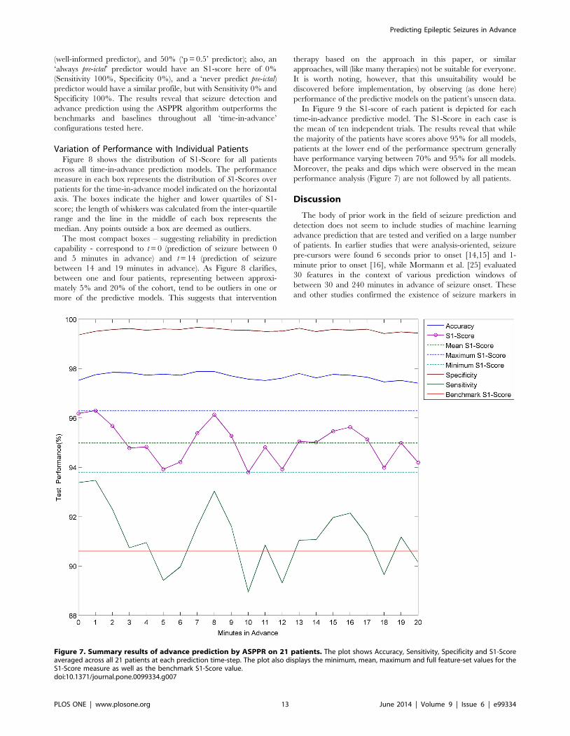
Mean Performance AnalysisSummary statistics for the performance of ASPPR are plotted in

Figure 7 and also shown in Table 1. Figure 7 shows, for each of the

21 ‘time in advance’ predictive models (from ‘t = 0’ to ‘t = 20’), the

mean values over the 21 patients of Accuracy, Specificity,

Sensitivity and S1-score, along with the benchmark performance

measure, and the overall minimum, maximum and mean of S1-

score. Accuracy and Specificity lay respectively in the ranges

[97.41%, 97.88%] and [99.36%, 99.67%], which are well above

the benchmark. The most well-informed random predictor would

achieve Accuracy of 63.0% and Specificity of 91.67%, represent-

ing the best of the baseline and random predictors (for example,

the ‘always pre-ictal’ predictor would achieve 5% Accuracy).

Sensitivity and S1-score also exhibit values that appear promising

with respect to further development towards intervention treat-

ments; however there is prominent variation between time-steps,

which is discussed later. Sensitivity is within the range [88.95%,

93.47%], with a standard deviation of 1.29%. S1-Score is within

the range [93.79%, 96.30%], with a lower standard deviation of

0.77%. In contrast, the Sensitivity of the well-informed random

predictor would be 8.33% (with Specificity 91.67% as above, and

S1-Score 15.2%); additionally, the Sensitivity of a ‘p = 0.5’ random

predictor would be 50%, but with Specificity dropping to 50%

(and S1-Score also at 50%). The S1-Score curve starts at t0 with

96.18% and rises a little at t = 1 to 96.30%, which is so far, the

highest observed value for advance prediction, and suggests that

prediction between 1 and 6 minutes in advance is more readily

achievable than prediction between 0 and 5 minutes in advance.

S1-score then decreases until it hits a trough at t = 5 with 93.92%,

rises to 96.13% at t = 8, and then dips to its lowest value at t = 10,

93.79%. It remains at or above 95% for t = 13, 14, 15, and

continues to stay above 94%. The red line in Figure 7 marks the

benchmark S1-score of 90.6% which was produced using the

default feature-set from the Costa et al. study [23]. Recall also that

baseline random predictor benchmarks for S1-score are 15.2%

(8)



(well-informed predictor), and 50% (‘p = 0.5’ predictor); also, an

‘always pre-ictal’ predictor would have an S1-score here of 0%

(Sensitivity 100%, Specificity 0%), and a ‘never predict pre-ictal)

predictor would have a similar profile, but with Sensitivity 0% and

Specificity 100%. The results reveal that seizure detection and

advance prediction using the ASPPR algorithm outperforms the

benchmarks and baselines throughout all ‘time-in-advance’

configurations tested here.

Variation of Performance with Individual PatientsFigure 8 shows the distribution of S1-Score for all patients

across all time-in-advance prediction models. The performance

measure in each box represents the distribution of S1-Scores over

patients for the time-in-advance model indicated on the horizontal

axis. The boxes indicate the higher and lower quartiles of S1-

score; the length of whiskers was calculated from the inter-quartile

range and the line in the middle of each box represents the

median. Any points outside a box are deemed as outliers.

The most compact boxes – suggesting reliability in prediction

capability - correspond to t = 0 (prediction of seizure between 0

and 5 minutes in advance) and t = 14 (prediction of seizure

between 14 and 19 minutes in advance). As Figure 8 clarifies,

between one and four patients, representing between approxi-

mately 5% and 20% of the cohort, tend to be outliers in one or

more of the predictive models. This suggests that intervention

therapy based on the approach in this paper, or similar

approaches, will (like many therapies) not be suitable for everyone.

It is worth noting, however, that this unsuitability would be

discovered before implementation, by observing (as done here)

performance of the predictive models on the patient’s unseen data.

In Figure 9 the S1-score of each patient is depicted for each

time-in-advance predictive model. The S1-Score in each case is

the mean of ten independent trials. The results reveal that while

the majority of the patients have scores above 95% for all models,

patients at the lower end of the performance spectrum generally

have performance varying between 70% and 95% for all models.

Moreover, the peaks and dips which were observed in the mean

performance analysis (Figure 7) are not followed by all patients.

Discussion

The body of prior work in the field of seizure prediction and

detection does not seem to include studies of machine learning

advance prediction that are tested and verified on a large number

of patients. In earlier studies that were analysis-oriented, seizure

pre-cursors were found 6 seconds prior to onset [14,15] and 1-

minute prior to onset [16], while Mormann et al. [25] evaluated

30 features in the context of various prediction windows of

between 30 and 240 minutes in advance of seizure onset. These

and other studies confirmed the existence of seizure markers in

Figure 7. Summary results of advance prediction by ASPPR on 21 patients. The plot shows Accuracy, Sensitivity, Specificity and S1-Scoreaveraged across all 21 patients at each prediction time-step. The plot also displays the minimum, mean, maximum and full feature-set values for theS1-Score measure as well as the benchmark S1-Score value.doi:10.1371/journal.pone.0099334.g007



advance of the actual onset, but did not attempt to (or failed to)

show notable predictive performance for a patient’s unseen EEG

data. Later prediction-oriented studies reported 68% Sensitivity

and 85% specificity for predictions up to 72 minutes prior to

seizure onset [22] trained and tested on 3–14 day recordings of 10

patients, and, for seizures up to 78 minutes in advance, 91%

Sensitivity and 85% specificity on the continuous EEG of only two

patients [21].

In this paper, ASPPR learns predictive models that are targeted

directly at recognizing patterns that occur in a specific 5-minute

window in advance of seizure onset. For each of 21 patients, 21

such models were learned, targeted respectively at ‘0 to 5 minutes

in advance’, ‘1 to 6 minutes in advance’, and so on up to the ’20 to

25 minutes in advance’ window. Feature selection (based on the ‘0

to 5 minutes in advance’ dataset for the specific patient) was done

prior to building these models, to extract the best 14 features for

that patient from a total of 204 features, and these 14 were then

used to build each individual predictive model via a Multi-Class

Support Vector Machine, incorporating an initial hyper-param-

eter selection phase.

The results suggest that all of the predictive models built by

ASPPR outperform both the benchmark feature set and baseline

predictors. Highlights include Sensitivity of 90.15% and Specificity

of 99.44% for prediction of seizure between 20 and 25 minutes in

advance (means taken over unseen data for each of the 21

patients), only a small amount less accurate than the Sensitivity of

93.38% and Specificity of 99.36% for prediction of seizure onset

between 0 and 5 minutes in advance.

With the summary S1-score performance measure for time-in-

advance predictive models t = 5 and t = 18 representing relatively

low points, and time-in-advance points t = 1 and t = 8 and t = 16

exhibiting local peaks, the findings revealed an intriguing apparent

periodicity with a wavelength between 7 and 8 minutes. This

periodicity could be related to infraslow oscillations that are

believed to be associated with sleep (which state we can tentatively

assume accounts for approximately one-third of the activity

recorded in the Freiburg data) and epilepsy. Vanhatalo et al.

[61] demonstrated large-scale infraslow oscillations during sleep in

the human cortex at wavelengths up to 50 seconds; these were

observed in widespread cortical regions, and strongly synchronized

with faster activities, as well as with inter-ictal epileptic events.

Related recent findings include those of Ren et al. [62] who

identified oscillations with wavelengths from 40 seconds to 120

seconds in three patients with refractory epilepsy occurring up to

22 minutes prior to clinical seizure onset, reflecting a dynamic

process during the pre-ictal state. Ren et al termed this process

‘very low frequency oscillation’ (VLFO), and suggested it may

render new insight into epileptogenesis and provide additional

information concerning the seizure prediction. Meanwhile, Parri

and Crunelli [63] reported calcium oscillations as slow as

0.003 Hz (corresponding to a wavelength approaching 6 minutes)

generated by thalamic astrocytes. Kaiser [64] suggests that, since

the astrocyte network manages energy and excitability in the

thalamus, this thalamic process may influence the thalamocortical

network and allow detection of corresponding infraslow frequen-

cies in the EEG. While the oscillatory behaviour observed in

Sensitivity and S1-score in Figures 7 and 8 may be partly artefact,

it could arise in part from a combination of infraslow oscillatory

processes (known to have large amplitude [61]), in at least some of

the patients, that interact to cause complex low-frequency-

dominated oscillations in the salience of signal patterns that are

discriminative in the context of the predictive models.

A further issue of interest is variation in the feature-sets

extracted for each patient in the first stage of building a predictive

Ta

ble

1.

Sum

mar

yo

fA

SPP

Ro

n2

1p

atie

nts

.

AC

C(%

)t

SP

(%)

tS

S(%

)t

S1

(%)

t

min

97

.41

20

99

.36

08

8.9

51

09

3.7

91

0

ma

x9

7.8

87

99

.67

79

3.4

71

96

.30

1

t=

09

7.5

20

99

.36

09

3.3

80

96

.18

0

t=

20

97

.41

20

99

.44

20

90

.15

20

94

.20

20

me

an

97

.68

99

.55

91

.14

94

.98

me

dia

n9

7.7

39

9.5

69

1.0

79

5.0

1

mo

de

97

.41

99

.36

88

.95

93

.79

std

0.1

40

.08

1.2

90

.77

ran

ge

0.4

70

.31

4.5

22

.51

Th

em

inim

um

(min

),m

axim

um

(max

),m

ean

,me

dia

n,m

od

e,s

tan

dar

dd

evi

atio

n(s

td)

and

ran

ge

of

the

fou

rm

eas

ure

so

fA

ccu

racy

(AC

C),

Spe

cifi

city

(SP

),Se

nsi

tivi

ty(S

S),S

1-S

core

(S1

)ar

elis

ted

.Ad

dit

ion

ally

,th

efo

ur

me

asu

res

atth

ese

izu

reo

nse

t(t

=0

)an

dat

the

larg

est

pre

dic

tio

nw

ind

ow

(t=

20

)h

ave

be

en

liste

d.T

he

‘t’c

olu

mn

for

eac

hm

eas

ure

lists

the

tim

ep

oin

to

fth

eco

rre

spo

nd

ing

stat

isti

calm

eas

ure

inm

inu

tes.

E.g

.th

em

inim

um

valu

efo

rA

ccu

racy

isat

tim

ep

oin

t2

0w

ith

valu

e9

7.4

1%

.d

oi:1

0.1

37

1/j

ou

rnal

.po

ne

.00

99

33

4.t

00

1



model for that patient. Variation in electrode placement,

individuals, and many other conditions during the data-procure-

ment process, make it difficult to expect high levels of overlap in

the feature sets for different patients. Indeed this was seen to be the

case. For example, the patient with the best mean S1-score at

‘t = 20’ (99.55%) was patient 9, whose feature-set comprised four

instances (from different channels) of SEF measured over the LTE

window, five instances of SBP features (at both STE and LTE

windows), along with three Skewness (LTE) and three Mean (LTE)

features. In contrast, patient 1 achieved the highest S1-Score

(99.61%) for the ‘t = 0’ predictive model, with a feature set

comprising (unlike patient 9), three of the Costa et al [23] features

(two signal energy STE and one signal energy LTE) along with

two instances of SEF features, six instances of SBP features, one

Skewness and two instances of Kurtosis. A core of three individual

features were however most common among the individual feature

sets; these were SEF (LTE), Accumulated Energy, and Skewness

(LTE), accounting respectively for 16.3%, 10.2% and 5.8% of the

204 ‘slots’ in the ‘top-14’ feature sets of the 21 patients. Meanwhile

STE features were clearly of lower predictive value than LTE

features, respectively accounting for 29.9% and 57.1% of slots,

while the feature categories of SBP and SEF respectively

accounted for 25.85% and 23.81% of slots. The two nonlinear

dynamics features took only 1.7% of slots.

The outcome of this study contributes further evidence of

advance seizure predictability. Further advances in performance

may well be available in future work that explores other ways to

extract discriminatory features from the EEG signals. For

example, the features we use are essentially univariate and

predominantly linear filters, but multivariate and other non-linear

filters may have advantages in this context. It should also be noted

that the feature-selection part of the comparative experiments

reported here was constrained to select a feature subset of size 14,

facilitating fair comparison with the benchmark. This is however

unlikely to be the optimal feature-subset size, and more successful

results for individual patients may well be achievable by allowing

the feature-subset size to vary in an unconstrained feature selection

step. This may, for example, lead to more favourable outcomes for

the 20% of individuals for whom the results are currently poor. It

is also worth examining the possibility of a different feature

selection stage for each separate time-in-advance model (rather

than, as here, one feature-set per patient). Meanwhile, we note

that the promising levels of Sensitivity and Specificity in our

results, combined with the fact that these results are obtained from

test data in the context of relatively large numbers of both

experiments and patients (in comparison with previous prediction-

oriented studies), arguably bodes well for future real-world

applications exploiting this technology for the benefit of epilepsy

patients.

Figure 8. Distribution of S1-scores over individual patients for each time-in-advance prediction model. The boxes at each intervaldisplay the distribution of average S1-Score of each of the 21 patients at each advance prediction time-step.doi:10.1371/journal.pone.0099334.g008



Acknowledgments

We are grateful to the Freiburg EEG Database [24] for making their data

available to the public and to EPILAB [34] for sharing their code with us.

Author Contributions

Conceived and designed the experiments: NM DWC. Performed the

experiments: NM. Analyzed the data: NM DWC. Contributed reagents/

materials/analysis tools: NM. Wrote the paper: NM DWC.

References

1. Mormann F, Andrzejak RG, Elger CE, Lehnertz K (2007) Seizure prediction:

the long and winding road. Brain 130: 314–333. doi:10.1093/brain/awl241.

2. Reynolds EH, Elwes R, Shorvon SD (1983) Why does epilepsy becomeintractable?: prevention of chronic epilepsy. The Lancet 322: 952–954.

3. Elger CE, Schmidt D (2008) Modern management of epilepsy: A practical

approach. Epilepsy & Behavior 12: 501–539. doi:10.1016/j.yebeh.2008.01.003.

4. Niedermeyer E, da Silva FHL (2005) Electroencephalography. Lippincott

Williams & Wilkins. 1 pp.

5. Noachtar S, Remi J (2009) The role of EEG in epilepsy: a critical review.

Epilepsy Behav 15: 22–33. doi:10.1016/j.yebeh.2009.02.035.

6. Baumgartner C, Serles W, Leutmezer F, Pataraia E, Aull S, et al. (1998) PreictalSPECT in temporal lobe epilepsy: regional cerebral blood flow is increased prior

to electroencephalography-seizure onset.

7. Adelson PD, Nemoto E, Scheuer M, Painter M, Morgan J, et al. (1999)Noninvasive Continuous Monitoring of Cerebral Oxygenation Periictally Using

Near-Infrared Spectroscopy: A Preliminary Report. Epilepsia 40: 1484–1489.

doi:10.1111/j.1528–1157.1999.tb02030.x.

8. Federico P (2005) Functional MRI of the pre-ictal state. Brain 128: 1811–1817.

doi:10.1093/brain/awh533.

9. Kerem DH, Geva AB (2005) Forecasting epilepsy from the heart rate signal.

Med Biol Eng Comput 43: 230–239. doi:10.1007/BF02345960.

10. Stein AG, Eder HG, Blum DE, Drachev A, Fisher RS (2000) An automateddrug delivery system for focal epilepsy. Epilepsy Research 39: 103–114.

11. Theodore WH, Fisher RS (2004) Brain stimulation for epilepsy. The Lancet

Neurology 3: 111–118. doi:10.1016/S1474-4422(03)00664-1.

12. da Silva FL, Blanes W, Kalitzin SN, Parra J, Suffczynski P, et al. (2003)

Epilepsies as Dynamical Diseases of Brain Systems: Basic Models of the

Transition Between Normal and Epileptic Activity. Epilepsia 44: 72–83.

doi:10.1111/j.0013-9580.2003.12005.x.

13. Viglione SS, Walsh GO (1975) Proceedings: Epileptic seizure prediction.

Electroencephalogr Clin Neurophysiol 39: 435–436.

14. Rogowski Z, Gath I, Bental E (1981) On the prediction of epileptic seizures. Biol

Cybern 42: 9–15. doi:10.1007/BF00335153.

15. Salant Y, Gath I, Henriksen O (1998) Prediction of epileptic seizures from two-

channel EEG. Med Biol Eng Comput 36: 549–556. doi:10.1007/BF02524422.

16. Siegel A, Grady CL, Mirsky AF (1982) Prediction of spike-wave bursts in

absence epilepsy by EEG power-spectrum signals. Epilepsia 23: 47–60.

17. Le Van Quyen M, Martinerie J, Baulac M, Varela F (1999) Anticipating

epileptic seizures in real time by a non-linear analysis of similarity between EEG

recordings. Neuroreport 10: 2149–2155.

18. Iasemidis LD, Sackellares JC, Zaveri HP, Williams WJ (1990) Phase space

topography and the Lyapunov exponent of electrocorticograms in partial

seizures. Brain Topogr 2: 187–201.

19. Litt B, Esteller R, Echauz J, D9Alessandro M, Shor R, et al. (2001) Epileptic

seizures may begin hours in advance of clinical onset: a report of five patients.

Neuron 30: 51–64. doi:10.1016/S0896-6273(01)00262-8.

20. Harrison MAF, Frei MG, Osorio I (2005) Accumulated energy revisited. Clinical

Neurophysiology 116: 527–531. doi:10.1016/j.clinph.2004.08.022.

Figure 9. Mean S1-Score of the ASPPR algorithm for 21 patients. The legend orders the patients in ascending order of their S1-Scoreaveraged over all time-steps.doi:10.1371/journal.pone.0099334.g009



21. Iasemidis LD, Shiau DS, Pardalos PM, Chaovalitwongse W, Narayanan K, et

al. (2005) Long-term prospective on-line real-time seizure prediction. ClinicalNeurophysiology 116: 532–544. doi:10.1016/j.clinph.2004.10.013.

22. Chaovalitwongse W, Iasemidis LD, Pardalos PM, Carney PR, Shiau DS, et al.

(2005) Performance of a seizure warning algorithm based on the dynamics ofintracranial EEG. Epilepsy Research 64: 93–113. doi:10.1016/j.eplepsyres.

2005.03.009.23. Costa RP, Oliveira P, Rodrigues G, Leitao B, Dourado A (2008) Epileptic

seizure classification using neural networks with 14 features: 281–288.

24. Epilepsy.uni-freiburg.de (2007) EEG Database — Seizure Prediction ProjectFreiburg. Available: https://epilepsy.uni-freiburg.de/freiburg-seizure-

prediction-project/eeg-database.25. Mormann F, Kreuz T, Rieke C, Andrzejak RG, Kraskov A, et al. (2005) On the

predictability of epileptic seizures. Clinical Neurophysiology 116: 569–587.doi:10.1016/j.clinph.2004.08.025.

26. Mormann F, Elger CE, Lehnertz K (2006) Seizure anticipation: from algorithms

to clinical practice. Current Opinion in Neurology 19: 187–193.27. Kononenko I (1994) Estimating attributes: analysis and extensions of RELIEF

Springer-Verlag New York, Inc.28. Chang C-C, Lin C-J (2011) LIBSVM: a library for support vector machines.

ACM Transactions on Intelligent Systems and Technology (TIST) 2: 27.

29. Uniklinik-freiburg.de (2013) Section for Epileptology, University Medical CenterFreiburg. Available: http://www.uniklinik-freiburg.de/epilepsie.html. Accessed

2014 May 18.30. EEGLAB (2011) EEGLAB - Open Source Matlab Toolbox for Electrophysi-

ological Research. Available: http://sccn.ucsd.edu/eeglab/. Accessed 2014 May18.

31. Chapelle O (2007) Training a support vector machine in the primal. Neural

Comput 19: 1155–1178. doi:10.1162/neco.2007.19.5.1155.32. Hand D, Mannila H, Smyth P (2001) Principles of data mining. Cambridge,

Mass.: MIT Press.33. Teixeira CA, Direito B, Feldwisch-Drentrup H, Valderrama M, Costa RP, et al.

(2011) EPILAB: A software package for studies on the prediction of epileptic

seizures. Journal of Neuroscience Methods 200: 257–271. doi:10.1016/j.jneumeth.2011.07.002.

34. Epilepsiae (2013) EPILAB Software - Epilepsiae. Available: http://www.epilepsiae.eu/project_outputs/epilab_software. Accessed 2014 May 18.

35. Prandoni P, Vetterli M (2008) Signal Processing for Communications. CRCPress. 1 pp.

36. Gigola S, Ortiz F, D9Attellis CE, Silva W, Kochen S (2004) Prediction of

epileptic seizures using accumulated energy in a multiresolution framework.Journal of Neuroscience Methods 138: 107–111. doi:10.1016/j.jneumeth.

2004.03.016.37. Daubechies I, Sweldens W (1998) Factoring wavelet transforms into lifting steps.

Journal of Fourier analysis and applications.

38. Schuster HG, Just W (2006) Deterministic Chaos. John Wiley & Sons. 1 pp.39. Kantz H, Schreiber T (2004) Nonlinear Time Series Analysis. 1 pp.

40. Ott E (2002) Chaos in Dynamical Systems. Cambridge University Press. 1 pp.41. Rosenstein MT, Collins JJ, De Luca CJ (1993) A practical method for

calculating largest Lyapunov exponents from small data sets. Physica D:Nonlinear Phenomena 65: 117–134. doi:10.1016/0167-2789(93)90009-P.

42. Kantz H (1994) A robust method to estimate the maximal Lyapunov exponent

of a time series. Physics Letters A 185: 77–87. doi:10.1016/0375-9601(94)90991-1.

43. Grassberger P, Schreiber T, Schaffrath C (1991) Nonlinear TimeSequence Analysis. Int J Bifurcation Chaos 01: 521–547. doi:10.1142/

S0218127491000403.

44. Grassberger P, Procaccia I (1983) Characterization of strange attractors. Phys

Rev Lett.

45. TSTOOL (2009) TSTOOL - Software packages for nonlinear time-series analysis.

Available: http://www.physik3.gwdg.de/tstool/. Accessed 2014 May 18.

46. De Clercq W, Lemmerling P, Van Huffel S, Van Paesschen W (2003)

Anticipation of epileptic seizures from standard EEG recordings. The Lancet

361: 971–971. doi:10.1016/S0140-6736(03)12780-8.

47. Martinerie J, Adam C, Le Van Quyen M, Baulac M, Clemenceau S, et al. (1998)

Epileptic seizures can be anticipated by non-linear analysis. Nat Med 4: 1173–

1176. doi:10.1038/2667.

48. Le Van Quyen M, Martinerie J, Navarro V, Baulac And M, Varela FJ (2001)

Characterizing neurodynamic changes before seizures. J Clin Neurophysiol 18:

191–208.

49. Quyen MLV, Navarro V, Martinerie J, Baulac M, Varela FJ (2003) Toward a

Neurodynamical Understanding of Ictogenesis. Epilepsia 44: 30–43.

doi:10.1111/j.0013-9580.2003.12007.x.

50. Chavez M, Le Van Quyen M, Navarro V (2003) Spatio-temporal dynamics

prior to neocortical seizures: amplitude versus phase couplings. IEEE

Transactions on Biomedical Engineering 50(5): 571–583.

51. MATLAB (1994) MATLAB – The Language of Technical Computing.

Available: http://www.mathworks.com/products/matlab. Accessed 2014 May

18.

52. Kononenko I, Simec E, Robnik-Sikonja M (1997) Overcoming the myopia of

inductive learning algorithms with RELIEFF. Applied Intelligence 7(1): 39–55.

53. Robnik-Sikonja M, Kononenko I (2003) Theoretical and empirical analysis of

ReliefF and RReliefF. Machine learning 53(1–2): 23–69.

54. Hsu CW, Chang CC, Lin CJ (2003) A practical guide to support vector

classification. University of National Taiwan.

55. Cortes C, Vapnik V (1995) Support-vector networks. Machine Learning 20(3):

273–297.

56. LIBSVM (2013) LIBSVM — A Library for Support Vector Machines.

Available: http://www.csie.ntu.edu.tw/,cjlin/libsvm/. Accessed 2014 May 18.

57. Knerr S, Personnaz L, Dreyfus G (1990) Single-layer learning revisited: a

stepwise procedure for building and training a neural network Berlin,

Heidelberg: Springer Berlin Heidelberg. pp. 41–50. doi:10.1007/978-3-642-

76153-9_5.

58. Krebel UHG (1999) Pairwise classification and support vector machines. MIT

Press. 14 pp.

59. Ben-Hur A, Weston J (2010) A user’s guide to support vector machines. In Data

mining techniques for the life sciences (pp. 223–239). Humana Press.

60. Winterhalder M, Schelter B, Schulze-Bonhage A, Timmer J (2006) Comment

on:‘‘Performance of a seizure warning algorithm based on the dynamics of

intracranial EEG’’. Epilepsy research 72(1).

61. Vanhatalo S, Palva JM, Holmes MD, Miller JW, Voipio J, et al. (2004) Infraslow

oscillations modulate excitability and interictal epileptic activity in the human

cortex during sleep. Proceedings of the National Academy of Sciences of the

United States of America, 101(14): 5053–5057.

62. Ren L, Terada K, Baba K, Usui N, Umeoka S, et al. (2011) Ictal very low

frequency oscillation in human epilepsy patients. Ann Neurol., 69: 201–206. doi:

10.1002/ana.22158

63. Parri HR, Crunelli V (2001) Pacemaker calcium oscillations in thalamic

astrocytes in situ. Neuroreport 12(18): 3897–3900.

64. Kaiser D (2013) Infralow Frequencies and Ultradian Rhythms. InSeminars in

pediatric neurology (Vol. 20, No. 4, pp. 242–245). WB Saunders.



https://epilepsy.uni-freiburg.de/freiburg-seizure-prediction-project/eeg-database

https://epilepsy.uni-freiburg.de/freiburg-seizure-prediction-project/eeg-database

http://www.uniklinik-freiburg.de/epilepsie.html

http://sccn.ucsd.edu/eeglab/

http://www.epilepsiae.eu/project_outputs/epilab_software

http://www.epilepsiae.eu/project_outputs/epilab_software

http://www.physik3.gwdg.de/tstool/

http://www.mathworks.com/products/matlab

http://www.csie.ntu.edu.tw/~cjlin/libsvm/

Predicting Epileptic Seizures in Advance

Documents

Transcript of Predicting Epileptic Seizures in Advance