Pathological pattern formation and cortical propagation of epileptic seizures

†Author for c

J. R. Soc. Interface (2005) 2, 113–127

doi:10.1098/rsif.2004.0028

Published online 21 February 2005

Received 23 NAccepted 29 J

Pathological pattern formation and corticalpropagation of epileptic seizures

Mark A. Kramer1, Heidi E. Kirsch2 and Andrew J. Szeri1,3,†

1Program in Applied Science and Technology, and 3Department of Mechanical Engineering,University of California, Berkeley, CA 94720-1740, USA

2Department of Neurology, University of California, San Francisco, CA 94143-0114, USA

The stochastic partial differential equations (SPDEs) stated by Steyn-Ross and co-workersconstitute a model of mesoscopic electrical activity of the human cortex. A simplification inwhich spatial variation and stochastic input are neglected yields ordinary differentialequations (ODEs), which are amenable to analysis by techniques of dynamical systemstheory. Bifurcation diagrams are developed for the ODEs with increased subcorticalexcitation, showing that the model predicts oscillatory electrical activity in a large range ofparameters. The full SPDEs with increased subcortical excitation produce travelling wavesof electrical activity. These model results are compared with electrocortical data recorded attwo subdural electrodes from a human subject undergoing a seizure. The model andobservational results agree in two important respects during seizure: (i) the averagefrequency of maximum power, and (ii) the speed of spatial propagation of voltage peaks. Thissuggests that seizing activity on the human cortex may be understood as an example ofpathological pattern formation. Included is a discussion of the applications and limitations ofthese results.

Keywords: mesoscopic cortical dynamics; dynamical systems theory; electrocorticogram;epilepsy; seizures; pattern formation

1. INTRODUCTION

Over 50 million people worldwide suffer from epilepsy, adebilitating condition of chronic unprovoked seizures.There exist many different classifications of seizures(e.g. simple partial seizures, complex partial seizures,generalized seizures), yet all seizures share the generalcharacteristic of inducing ahyperexcitation of the cortex(the outer fewmillimetres of the brain). Themicroscopicbehaviour of individual cortical neurons during thishyperexcitation is well documented and is the basis forsome drug treatments. However, comprehensive micro-scopic recordings are infeasible, especially in humanpatients. Therefore, physicians record the macroscopicelectrical behaviour of the seizing human cortex andcollect the scalp electroencephalogram (EEG) andelectrocorticogram (ECoG). At this macroscopic level,which involves interactions between millions of individ-ual neurons, cortical seizures are less well understood(Quyen et al. 2003).

In this paper, we describe a model of the mesoscopicelectrical behaviour of the seizing human cortex. Weemploy a recently developed continuum model ofcortical electrical activity, which consists of a systemof stochastic partial differential equations (SPDEs;Steyn-Ross et al. 2003). These SPDEs (and the relatedordinary differential equations; ODEs) have beensuccessfully applied to study the electrical properties

orrespondence ([email protected]).

ovember 2004anuary 2005

113

of the anaesthetized human cortex (i.e. the anaestheto-dynamicmodel of cortical function). In a series of papers,Steyn-Ross and colleagues showed that the modelequations predict changes in the scalp EEG of anaes-thetized patients consistent with experimental results(Steyn-Ross et al. 1999, 2001a,b, 2003).

Here, we consider whether these SPDEs can modelthe mesoscopic electrical behaviour recorded from thehuman cortex during a seizure. Our methods differ fromprevious discussions. We do not assume that somevariables equilibrate much faster than others (the slow-membrane or adiabatic approximation; Steyn-Rosset al. 1999), nor do we apply techniques of stochasticcalculus (such as the Ornstein–Uhlenbeck equation) tothe linearized SPDEs (Steyn-Ross et al. 2003). Instead,we approach the SPDEs from a dynamical systemsperspective and employ ideas and tools from bifur-cation theory. We show that in some parameterregimes, the SPDEs predict pathological oscillatorybehaviour—characterized by a bifurcation to a large-amplitude, coherent travelling wave against a back-ground of spatio-temporal fluctuations—in someimportant ways consistent with ECoG recordingsfrom the seizing cortex.

The organization of this paper is as follows. In §2, wediscuss clinical ECoG data recorded at two subduralelectrodes from a human subject during his typicalcomplex partial seizures. In §3, we review the modelequations, the dimensionless SPDEs we use here, andthe variable of principal interest: the excitatory mean

q 2005 The Royal Society

114 Pattern formation and cortical propagation M. A. Kramer and others

soma potential he. In §4, we consider a simplifiedversion of the SPDEs that possesses neither spatialvariance nor stochastic input; we call this system thedimensionless ODEs. In §§4.1 and 4.2, we computebifurcation diagrams for the dimensionless ODEs attwo different parameter values. We show that in bothcases oscillatory activity (as expected during a seizure)occurs. For typical parameter values, the oscillatoryactivity is unstable and short-lived. For other par-ameter values (which may be consistent with theseizing cortex), the oscillatory activity is stable andlong-lived. In §5, we analyse the complete dimension-less SPDEs. We show that results from this systemagree qualitatively with results from the simplerdimensionless ODEs, and that travelling wave solutionsexist. In §6, we compare the model solutions with theexperimental recordings, and in §7, we discuss theseresults.

2. OBSERVATIONAL DATA: ECoG SEIZURERECORDINGS

The cellular mechanisms of a seizure have beenextensively studied and some general microscopiccharacteristics have been deduced (Dichter & Ayala1987). Preceding a seizure, thousands of individualneurons in the seizure focus (the brain region where aseizure begins, also known as the epileptogenic zone)undergo depolarization shifts followed by an after-hyperpolarization. As long as this behaviour is confinedto the seizure focus, there may be no clinical manifes-tation (although this synchronous activity can bedetected as an interictal spike or a sharp wave in theEEG or ECoG). Gradually, as the seizure develops, themagnitude of the afterhyperpolarization decreases andindividual neurons generate nearly continuous actionpotentials. The inhibition surrounding the seizure focusweakens, the seizure spreads to other cortical neurons,and a clinical seizure occurs. Here, we will not considerthis microscopic behaviour of individual neurons, norwill we consider ictogenesis (the initiation of theseizure, which may occur in deeper brain regions).Instead, we investigate the mesoscopic characteristicsof seizure activity on the cortical surface as mademanifest in subdural ECoG recordings.

Large amounts of ECoG data are often recordedfrom the seizing cortex (i.e. ictal data) as part of clinicalcare of patients with intractable epilepsy. Thesepatients whose seizures do not respond well to drugtreatments may undergo surgery to remove a region ofcortex that is believed to contain the seizure focus. Suchresective surgery offers a chance to eliminate orameliorate the seizures. In the process of planningsuch surgery, clinicians must accurately locate theseizure focus, and identify any surrounding areas offunctional cortex that should be preserved to minimizepost-operative deficits. If necessary, to define theseizure focus more precisely with respect to structuraland functional anatomy, clinicians may implant sub-dural electrodes on the brain surface for extended timeperiods (typically one week) to obtain recordingsduring seizures and locate the seizure onset. Theelectrodes are placed over the region of cortex suspected

J. R. Soc. Interface (2005)

to contain the seizure focus based on: (i) semiologicfeatures of the patient’s seizures (i.e. the observablefeatures of the seizure, such as eye deviation or limbjerking), (ii) scalp EEG recordings made during typicalseizures, (iii) abnormalities observed in the ECoGrecorded intraoperatively at the time of electrodeimplantation (i.e. interictal recordings), or (iv)abnormalities seen on brain images. After the electro-des are implanted and the patient experiences his or hertypical seizures, physicians locate the seizure focusthrough visual analysis of the ECoG recordings andformulate the surgical plan.

In this paper, we consider data collected from a49-year-oldmalewhohad electrode implantation as partof his care at the University of California, San Francisco(UCSF) Epilepsy Center. He had medically refractorycomplex partial seizures that began with staring andmanual automatisms and frequently generalized intoconvulsions. Prior scalp EEG recordings had suggestedthat his seizures originated in the right temporal lobe,but MRI showed left mesial temporal sclerosis, raisingthe possibility that his seizures arose from the lefttemporal lobe instead. To better lateralize seizure onset,subdural and depth electrodes were implanted, withsubdural electrode strips placed over the left and rightlateral frontal regions and the left and right subtemporalregions. In addition, bilateral hippocampal depthelectrodes were placed, although we will not discussthese hippocampal recordings here. Each subduralelectrode strip contained six 4 mm diameter platinum–iridium discs arrayed in a single row, embedded in a1.5 mm thick silastic sheet with 2.3 mm diameterexposed surfaces and 10 mm spacing between the discs.After electrode implantation, the patientwas brought tothe video–telemetry unit, where his antiseizure medi-cations were slowly withdrawn. ECoG data wererecorded continuously at 400 Hz from all electrodes for5.5 days. During this time, observations of eight typicalseizures were captured. These recordings were of goodquality andwere determined, based on clinical review byboard-certified clinical neurophysiologists, to showseizure onset from right medial temporal regions, witha pattern characteristic of seizures arising from thisregion. The patient went on to have a right anteriortemporal lobectomy based on these clinical data.

ECoG epochs containing six of the patient’s seizureswere extracted from the clinical record and reviewed forresearch purposes in accordance with UCSF andUniversity of California, Berkeley human subjectsguidelines. (Two of the seizure data files were corruptedand no longer available for extraction.) In figure 1,we show ECoG data leading up to and during a seizurerecorded at two neighbouring subdural electrodesabove the right lateral frontal region. We refer tothe time-series recorded at these two electrodes asX (lower curve) and Y (upper curve). The ECoG datashown in this figure possess three notable features.First, we observe that large-amplitude voltage oscil-lations occur during the seizure (tO17.5 s). Wedetermine the frequency of these oscillations bycomputing the windowed power spectrum (WPS) of Xand Y. To compute the WPS, we partition the 50 s ofdata plotted in figure 1 into 100 overlapping windows of

(a)

(b)

323028

time (s)

262422

0

– 500volta

ge (

µV)

volta

ge (

µV)

0

500

– 500

0

500

10 20 30 40 50

Figure 1. ECoG data recorded at two neighbouring subdural electrodes (separated by 10 mm) located on the surface of the rightlateral frontal lobe. We label the time-series X (lower trace in each figure) and Y (upper trace in each figure). To ease visualcomparison we subtract 400 mV fromX and add 400 mV toY. (a) Here, we show 50 s of ECoG activity recorded at two electrodes.There are three regions of ECoG activity: normal ECoG activity (0 s!t!14 s), followed by voltage suppression (14 s!t!17.5 s), and seizure (tO17.5 s). (b) Here, we show the data from (a) for 22 s!t!32 s. We note that initially oscillations in X andY have the same shape, and that oscillations in X are of larger magnitude and appear to precede those in Y. For tO27 s therelationship between X and Y becomes more complicated.

101

10

20time (s) time (s)

freq

uenc

y (H

z)

30 40 50 10 20 30 40 50

(a) (b)

Figure 2. The windowed power spectra (WPS) for the two ECoG time-series shown in figure 1. Here, subfigures (a) and(b) correspond to the time-series X and Y in figure 1, respectively. The WPS are plotted in logarithmic greyscale with black andwhite denoting regions of high power (greater than 30 mV2) and low power (less than 0.03 mV2), respectively. The vertical line inthe figure at tZ17.5 s denotes the approximate onset of seizure.

Pattern formation and cortical propagation M. A. Kramer and others 115

1.0 s duration and 0.5 s overlap. For example, the firstwindow includes data for 0.0 s%t%1.0 s, the second0.5 s%t%1.5 s, the third 1.0 s%t%2.0 s and so on.We then multiply the data in each window by theHanning function and compute the power spectrum.We plot the WPS results for X and Y in figure 2a,b,respectively. The horizontal axis in each figure corres-ponds to the centre times of the windows, and the solidvertical line to the time of seizure onset. We note, in theseconds preceding the seizure, the suppression of power


at both electrodes for all frequencies. After seizureonset, the regions of largest power occur at frequenciesbetween 1 and 10 Hz. The second notable feature in theobserved data is the abrupt transition from normalECoG activity (for t!14 s) to seizing activity (fortO17.5 s). This can be observed both in the originaltime-series data (figure 1a) and in the WPS (figure 2).Lastly, we find that the oscillations recorded at the twoelectrodes are slightly out of phase. One may deducethis conclusion directly from figure 1b; we note that

��

��

��

�

��

��

��

��

��

��

�

��

Figure 3. The windowed cross-correlation between the two ECoG time-series shown in figure 1. The WCC are plotted in lineargreyscale with regions of strong correlation (greater than 0.8) and anticorrelation (less than K0.8) denoted by black and white,respectively. The vertical line in the figure at tZ17.5 s denotes the approximate onset of seizure. The horizontal line in the figuredenotes the zero lag.


peaks in the oscillations in X (lower trace) appear toprecede those in Y (upper trace) until tz29 s. At thispoint, the relationship between the two time-seriesbecomes more complicated. To determine how thephase relationship between these two electrodeschanges over time, we compute the windowed cross-correlation (WCC). In a manner similar to the WPScalculation, we partition the data into overlappingwindows and compute the cross-correlation between Xand Y in each window. We show the results in figure 3.Following seizure onset (denoted by the vertical line inthe figure), two regions of strong correlation occur:the first from 17.5 s!t!27 s, and the second from28 s!t!50 s. In the first region, X leads Y (i.e. the lagtime is positive) while in the second region, X lags Y(i.e. the lag time is negative but near zero). In §6, wequantify the WPS and WCC results for six seizuresrecorded from the subject. We compare these resultswith the solutions to the SPDEs, discussed in §3.

3. MODEL: DIMENSIONLESS SPDEs

An ideal model of the human cortex would describe theelectrical behaviour of each individual neuron and itssurrounding extracellular environment. This discretemodel—applied over the entire three-dimensionalcortex—would contain over 1010 dynamical variablesand would be intractable. Fortunately, the physiologyof the cortex (e.g. dense local connections) andnumerous experimental results suggest that neuronsact in populations or assemblies (Singer 1993; Singer &Gray 1995). Moreover, most methods for observing thehuman cortex (e.g. the ECoG time-series of interest inthis work) record the summed electrical activity frompopulations of order 105 cortical neurons (Nunez 1995).For these reasons, researchers have developed conti-nuum models of cortical electrical activity.

Such continuum models are not new; some of theearliest were developed by Freeman (1964) and


Wilson & Cowan (1972, 1973). Here, we utilize thesystem of SPDEs stated by Steyn-Ross et al. (2003).These SPDEs were introduced in Steyn-Ross et al.(1999), where the authors included stochastic input tothe system of PDEs first stated by Liley et al. (1999).To develop this model, Liley et al. (2002) considered aspatially averaged approximation to the humancortex. Microscopic elements (like individual neurons)were averaged over columnar volumes (perpendicularto the cortical surface) whose diameter was chosen tolie below the spatial resolution of EEG or ECoGrecordings. The resulting mesoscopic model (with theaddition of stochastic input) consists of 14 coupled,nonlinear SPDEs (Steyn-Ross et al. 2003).

By solving the SPDEs in Steyn-Ross et al. (2003)numerically, one computes solutions for all 14 variablesas functions of space and time. One of these variables,he, is the spatially averaged excitatory soma membranepotential. Researchers have demonstrated that thedeviation of he from rest is proportional to the sign-reversed value of the extracellular local field potential(LFP). Because the ECoG represents the spatiallyaveraged LFP, we assume that he is linearly related tothe ECoG (Liley et al. 2002). In this way, the modelvariable he is related to the observational ECoG data. Inwhat follows, we compare he calculated in numericalsolutions to the SPDEs with ECoG data recordedduring seizure. We show that increasing the subcorticalexcitatory input to the model cortex produces be-haviour in he that mimics ECoG data recorded from theseizing cortex.

In appendix A, we discuss a procedure to non-dimensionalize the SPDEs and associated functions.The main advantage of recasting the equations indimensionless form is a reduction in the number ofparameters. There are 20 parameters in the dimen-sionless SPDEs whereas in the original SPDEs thereare 29. We define each dimensionless variable andparameter in terms of its dimensional counterparts

Table 1. Dynamical variable definitions for the dimensionlessSPDEs neural macrocolumn model.(The dimensionless variables (left column) are defined interms of the dimensional symbols (middle column) found intable 1 of Steyn-Ross et al. (2003). The variables are describedin the right column. Subscripts e and i refer to excitatory andinhibitory.)

symbol definition description

~he;i he,i/hrest population mean soma

dimensional electricpotential

~I ee;ie Iee,iege/(Geexp(1)Smax) total e/e, i/e input

to excitatory synapses~I ei;ii Iei,iigi/(Giexp(1)S

max) total e/i, i/i input toinhibitory synapses

~fe;i fe,i/Smax long range

(corticocortical) inputto e, i populations

~t t/t dimensionless time

~x x=ðt~vÞ dimensionless space


from Steyn-Ross et al. (2003) in tables 1 and 2,respectively. In what follows, we study a simplifiedODE version of the dimensionless model in §4, andcompute numerical solutions to the complete dimen-sionless SPDE model in §5. Readers less interested inthe mathematical details may like to skip to §6 wherewe compare the model solutions and observationalresults.

4. SIMULATIONS: DIMENSIONLESS ODEs

Our goal is to determine whether the dimensionlessSPDEs in equation (A 1a–h) can be used to model themesoscopic electrical activity observed on the seizingcortical surface, as discussed in §2. However, the size ofthe system (14 first-order differential equations and 20parameters), the stochastic input in equation (A 1c–f )and the spatial dependence in equation (A 1g,h) makethis a challenging model. Therefore, to gain whatinsight we can from a simpler model, we ignore for themoment the spatial dependence and stochastic input inequation (A 1a–h). The resulting equations form asystem of ODEs, which we call the dimensionlessODEs. Although there are many tools available forthe study of ODEs, we use AUTO (continuation andbifurcation software for ODEs) to determine fixedpoints, their stability type, limit cycles and bifurcationsin the phase portraits (Doedel et al. 2000).

During a seizure, the cortex typically enters a stateof hyperexcitation, manifest in ECoG data throughlarge-amplitude oscillations (Niedermeyer & DaSilva1999). This activity corresponds to spatially coherentoscillations in the variable he. In this direction, weinvestigate whether oscillations in he occur in thedimensionless ODEs owing to changes in the excitatoryparameters. We note that different types of seizuresproduce different oscillatory patterns in EEG andECoG recordings (Spencer et al. 1992; Ebersole &Pacia 1996). Here, we seek to model the seizing cortexin a qualitative way suggestive of the typical ECoG


data shown in figure 1. Specifically, we require that:(i) the model produces stable oscillations in he, (ii) thefrequency of the oscillations agree (roughly) withclinical observations, and (iii) the transition to oscil-latory behaviour occurs abruptly.

The general statement that increased excitation (ordecreased inhibition) incites cortical seizure activitymasks the numerous associated physiological changesthat occur in the seizing neuronal assemblies (Dichter &Ayala 1987; Morimoto et al. 2004). At the cellular level,these physiological changes are observed in experimentand can be compared to results computed from detailedcomputational models of a single neuron (Traub et al.2001). It is not clear how the cellular mechanisms orsingle neuron models relate to mesoscopic seizurerecordings or continuum models. Seizures induced inanimal models allow mesoscopic ECoG recordings andsome control over parameters related to continuummodels. For example, Freeman (1992) discusses elec-trocortical data recorded from a seizing animal’solfactory bulb. He compares these recordings with hisKIII model of the olfactory system and finds that aparameter connecting excitatory subsets of the modelmust increase to induce seizures. Analogies betweensuch animal models and human seizure activity can bemade but, as for the cellular models, these relationshipsare not clear.

In our analysis, we vary only two parameters, Pee

and Ge, both related to the excitation of the model. Wechoose these parameters for two reasons. First, asmentioned previously, the general claim that increasedexcitation incites seizures is well known. Thus, weselect two parameters related to the excitation of themodel. Second, an increase in the level of the membranepotential of a neuronal population is thought to be animportant control factor in inducing seizures (Dichter& Ayala 1987; da Silva et al. 2003). We show thatincreases in Ge raise the excitatory mean soma potentialhe of the stable fixed points. A similar result holds forPee but is not shown. We fixed the remaining 18dimensionless parameters at the typical values shownin table 2. In terms of dimensional variables, thedimensionless parameterPee is: (i) directly proportionalto pee (the subcortical excitatory spike input to theexcitatory neurons of the cortex), and (ii) inverselyproportional to Smax (the maximum firing rate inducedby the soma voltage). Thus, an increase in Pee

represents either an increase in the subcortical exci-tation of the cortex or a decrease in the maximum firingrate. To model an increase in excitatory input (from asubcortical region, such as the thalamus) to the cortex,the parameter Pee is increased. The dimensionlessparameter Ge is: (i) directly proportional to Smax andGe (the peak excitatory postsynaptic potential; EPSP),and (ii) inversely proportional to ge (the EPSPneurotransmitter rate constant) and jhreve Khrestj (themagnitude of the difference between the excitatoryreversal and resting potentials). Thus, an increase in Ge

represents either an increase in peak EPSP amplitudeor maximum firing rate, or a decrease in the differencebetween the excitatory reversal and resting potentialsor the EPSP neurotransmitter rate constant. The lattercorresponds to an increase in the EPSP duration. We

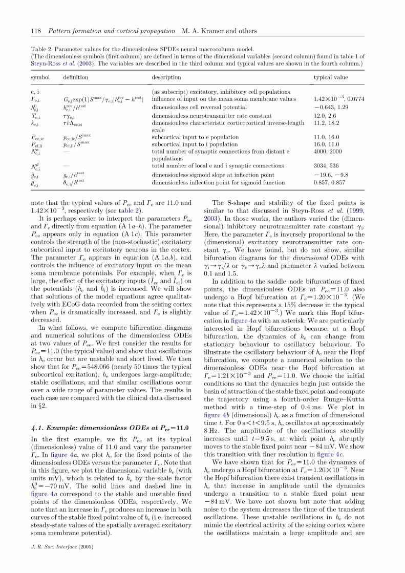
Table 2. Parameter values for the dimensionless SPDEs neural macrocolumn model.(The dimensionless symbols (first column) are defined in terms of the dimensional variables (second column) found in table 1 ofSteyn-Ross et al. (2003). The variables are described in the third column and typical values are shown in the fourth column.)

symbol definition description typical value

e, i (as subscript) excitatory, inhibitory cell populationsGe,i Ge;iexpð1ÞSmax=ge;ijhreve;i Khrestj influence of input on the mean soma membrane values 1.42!10K3, 0.0774

h0e;i hreve;i =hrest dimensionless cell reversal potential K0.643, 1.29

Te,i tge,i dimensionless neurotransmitter rate constant 12.0, 2.6le,i t~vLee;ei dimensionless characteristic corticocortical inverse-length

scale11.2, 18.2

Pee,ie pee,ie/Smax subcortical input to e population 11.0, 16.0

Pei,ii pei,ii/Smax subcortical input to i population 16.0, 11.0

Nae;i — total number of synaptic connections from distant e

populations4000, 2000

Nbe;i

— total number of local e and i synaptic connections 3034, 536

~ge;i ge,i/hrest dimensionless sigmoid slope at inflection point K19.6, K9.8

~qe;i qe,i/hrest dimensionless inflection point for sigmoid function 0.857, 0.857


note that the typical values of Pee and Ge are 11.0 and1.42!10K3, respectively (see table 2).

It is perhaps easier to interpret the parameters Pee

and Ge directly from equation (A 1a–h). The parameterPee appears only in equation (A 1c). This parametercontrols the strength of the (non-stochastic) excitatorysubcortical input to excitatory neurons in the cortex.The parameter Ge appears in equation (A 1a,b), andcontrols the influence of excitatory input on the meansoma membrane potentials. For example, when Ge islarge, the effect of the excitatory inputs (~I ee and ~I ei) onthe potentials (~he and ~hi) is increased. We will showthat solutions of the model equations agree qualitat-ively with ECoG data recorded from the seizing cortexwhen Pee is dramatically increased, and Ge is slightlydecreased.

In what follows, we compute bifurcation diagramsand numerical solutions of the dimensionless ODEsat two values of Pee. We first consider the results forPeeZ11.0 (the typical value) and show that oscillationsin he occur but are unstable and short lived. We thenshow that for PeeZ548.066 (nearly 50 times the typicalsubcortical excitation), he undergoes large-amplitude,stable oscillations, and that similar oscillations occurover a wide range of parameter values. The results ineach case are compared with the clinical data discussedin §2.

4.1. Example: dimensionless ODEs at PeeZ11.0

In the first example, we fix Pee at its typical(dimensionless) value of 11.0 and vary the parameterGe. In figure 4a, we plot he for the fixed points of thedimensionless ODEs versus the parameter Ge. Note thatin this figure, we plot the dimensional variable he (withunits mV), which is related to ~he by the scale factorh0eZK70 mV. The solid lines and dashed line infigure 4a correspond to the stable and unstable fixedpoints of the dimensionless ODEs, respectively. Wenote that an increase in Ge produces an increase in bothcurves of the stable fixed point value of he (i.e. increasedsteady-state values of the spatially averaged excitatorysoma membrane potential).


The S-shape and stability of the fixed points issimilar to that discussed in Steyn-Ross et al. (1999,2003). In those works, the authors varied the (dimen-sional) inhibitory neurotransmitter rate constant gi.Here, the parameter Ge is inversely proportional to the(dimensional) excitatory neurotransmitter rate con-stant ge. We have found, but do not show, similarbifurcation diagrams for the dimensional ODEs withgi/gi/l or ge/gel and parameter l varied between0.1 and 1.5.

In addition to the saddle–node bifurcations of fixedpoints, the dimensionless ODEs at PeeZ11.0 alsoundergo a Hopf bifurcation at GeZ1.20!10K3. (Wenote that this represents a 15% decrease in the typicalvalue of GeZ1.42!10K3.) We mark this Hopf bifur-cation in figure 4a with an asterisk. We are particularlyinterested in Hopf bifurcations because, at a Hopfbifurcation, the dynamics of he can change fromstationary behaviour to oscillatory behaviour. Toillustrate the oscillatory behaviour of he near the Hopfbifurcation, we compute a numerical solution to thedimensionless ODEs near the Hopf bifurcation atGeZ1.21!10K3 and PeeZ11.0. We choose the initialconditions so that the dynamics begin just outside thebasin of attraction of the stable fixed point and computethe trajectory using a fourth-order Runge–Kuttamethod with a time-step of 0.4 ms. We plot infigure 4b (dimensional) he as a function of dimensionaltime t. For 0 s!t!9.5 s, he oscillates at approximately8 Hz. The amplitude of the oscillations steadilyincreases until tZ9.5 s, at which point he abruptlymoves to the stable fixed point nearK84 mV. We showthis transition with finer resolution in figure 4c.

We have shown that for PeeZ11.0 the dynamics ofhe undergo a Hopf bifurcation at GeZ1.20!10K3. Nearthe Hopf bifurcation there exist transient oscillations inhe that increase in amplitude until the dynamicsundergo a transition to a stable fixed point nearK84 mV. We have not shown but note that addingnoise to the system decreases the time of the transientoscillations. These unstable oscillations in he do notmimic the electrical activity of the seizing cortex wherethe oscillations maintain a large amplitude and are

0 0 2 4 6 8 10 12–100

–80

–60

–40

–20

0.002 0.004

Ge

h e (m

V)

0.006 0.008

t (s)

(a) (b)

–100

–80

–60

–40

–20

h e (m

V)

(c)

t (s)8.0 8.5 9.0 9.5 10.0 10.5 11.0

Figure 4. (a) Bifurcation diagram for the dimensionless ODEs at PeeZ11.0. As the dimensionless parameter Ge is varied, thestable (solid lines) and unstable (dashed line) fixed points in he of the dimensionless ODEs are shown. The asterisk denotes theHopf bifurcation. There are two saddle–node bifurcations also visible in the figure. (b) Numerical solution to the dimensionlessODEs at GeZ1.21!10K3 and PeeZ11.0, near the Hopf bifurcation shown in (a). Dimensional he is plotted as a function ofdimensional time t. The oscillations in he increase in amplitude until the oscillations cease and he/K84 mV. (c) The transitionfrom transient oscillatory motion in he to the fixed point at finer resolution.


necessarily stable to incessant perturbations from othercortical, as well as deeper, brain regions.

4.2. Example: dimensionless ODEsat PeeZ548.066

Here, we consider an example more closely related tothe seizing cortex. To increase the excitation of themodel cortex, we fix PeeZ548.066 (nearly 50 times thetypical value). This can be interpreted as increasedexcitatory input from deeper brain regions to thecortex, say. As in §4.1, we vary the parameter Ge andplot in figure 5a the bifurcation diagram in he for thedimensionless ODEs. The solid lines and dashed line infigure 5a correspond to stable and unstable fixed pointsof the dimensionless ODEs, respectively, and theasterisks to Hopf bifurcations. We note that an increasein Ge produces an increase in both curves of stablefixed points of he.

There are additional curves in figure 5a absent fromfigure 4a. These curves indicate the extremal values andstability type of the limit cycles born in the Hopfbifurcations. The dash–dot lines in figure 5a representthe maxima and minima of he achieved during a stable


limit cycle. The dotted lines represent the maxima andminima of he achieved during an unstable limit cycle.Thus, for 0.67!10K3!Ge!0.96!10K3, the dynamicsof he feature a stable limit cycle of large amplitude. Wenote that a 32% decrease in the typical value ofGeZ1.42!10K3 is required to enter this range. Thestable, oscillatory behaviour of he satisfies one of ourcriteria for modelling the seizing cortex.

To illustrate the stable oscillations in he for 0.67!10K3!Ge!0.96!10K3, we compute a numerical sol-ution to the dimensionless ODEs at GeZ0.96!10K3

and PeeZ548.066 using the fourth-order Runge–Kuttamethod with a time-step of 0.4 ms. In figure 5b, we plothe (with dimensions mV) as a function of dimensionaltime t. After an initial transient, he is entrained by alarge-amplitude limit cycle with a dominant frequencynear 7.5 Hz. We note that these oscillations arenot sinusoidal. The frequency of the he oscillationsis qualitatively consistent with the clinical observationsfrom a seizing patient shown in figure 1.

The true environment of the human cortex iscontinually changing, for example, in response tosensory stimuli. Therefore, any model of the seizingcortex must behave properly over a broad range of

0–100

–80

–60

–40

–20

–100

–80

–60

–40

–20

0.0005 0.0010

Ge

t (s)

h e (m

V)

h e (m

V)

0.0015

0 0.5 1.0 1.5 2.0 2.5 3.0

(a)

(b)

Figure 5. (a) Bifurcation diagram for the dimensionless ODEsat PeeZ548.066. The parameter Ge is varied and the stable(solid lines) and unstable (dashed line) fixed points in he areshown. The asterisks denote the two Hopf bifurcations.The dash–dot lines denote the maximum and minimumvalues of he achieved during a stable limit cycle. The dottedlines denote the maximum andminimum values of he achievedduring an unstable limit cycle. The branch of limit cycles isborn and dies in two subcritical Hopf bifurcations; twosaddle–node bifurcations of limit cycles lead to large-amplitude stable oscillations with sudden onset. (b) Numeri-cal solution to the dimensionless ODEs at GeZ0.96!10K3

and PeeZ548.066, near the rightmost Hopf bifurcation in (a).Dimensional he is plotted as a function of dimensional time t.The oscillations in he occur at a frequency near 7.5 Hz and arestable to perturbations.

0.0006

200

400

600

800

1000

0.0008Ge

Pee

0.0010 0.0012

Figure 6. The difference between the maximum and minimumachieved by (the dimensional) he in solutions of thedimensionless ODEs for parameters Pee and Ge. The differenceis plotted in linear greyscale with white representing a 0 mVdifference and black representing a 50 mV difference. Thedark region corresponds to stable oscillations of he andbroadens as Pee is increased. The parameter values used tocreate figure 5b (GeZ0.96!10K3 and PeeZ548.066) are nearthe centre of this figure.


parameter values. Here, we require that oscillatoryactivity in he occur over extended regions of theparameters Pee and Ge. To confirm this, we computenumerical solutions to the dimensionless ODEs for11.0!Pee!1000.0 and 0.5!10K3!Ge!1.4!10K3

using the fourth-order Runge–Kutta method with atime-step of 0.4 ms. We then determine the differencebetween the maximum and minimum achieved by thesolution he after transient behaviour has decayed. Ifhe approaches a fixed point, then the maximum andminimum are nearly equal and their differenceapproaches zero. However, if he is entrained by a limitcycle (e.g. figure 5b), then the difference between themaximum and minimum achieved by he is non-zero.In figure 6, we plot the difference between the maximum


and minimum achieved by he as a function of theparameters Pee and Ge. The difference is plotted ingreyscale with white representing a 0 mV difference andblack representing a 50 mV difference. We find thatoscillations in he (represented by the dark regions infigure 6) extend over a broad range of parameter valuesbeginning near PeeZ250.0 and GeZ1.3!10K3. Theseregions of oscillatory activity in he illustrate theparameter values at which the dimensionless ODEs‘seize’. We have found that the Hopf bifurcation (andthus the oscillatory activity) is born in a codimensiontwo bifurcation of the Takens–Bogdanov type atPeeZ53.2 and GeZ2.98!10K3 (Kramer 2005). Wenote that increasing Pee, and thus raising the sub-cortical excitatory input to the model cortex, enlargesthe region of Ge over which oscillations in he occur.

5. SIMULATION: DIMENSIONLESS SPDEs

We have considered in some detail the dimensionlessODEs. There is no direct conclusion that the analysis ofthis simplified system allows one to draw for the fulldimensionless SPDEs. The stochastic inputs or thespatially distributed dynamics may destroy the inter-esting features we observed in the dimensionless ODEs.We have shown in §4.2 that the dimensionless ODEsundergo a Hopf bifurcation near PeeZ548.066 and

GeZ0.96!10K3, and that oscillations in he persist overa broad region of parameter values. Here, we shallexamine whether the full dimensionless SPDEsexhibit similar oscillatory behaviour. We will considerthree examples. For each example, we computenumerical solutions to the dimensionless SPDEs usingthe Euler–Maruyama algorithm with fixed steps inspace and time, 14 mm and 0.1 ms, respectively(Higham 2001). We consider only one spatial dimension~x; the system can now be visualized as describing a lineof closely spaced electrodes, such as the strip of

x (mm) x (mm)

2500

3000

2000

1500t (m

s)

1000

500

00 100 200 300 400 500 600 0 100 200 300 400 500 600

(a) (b)

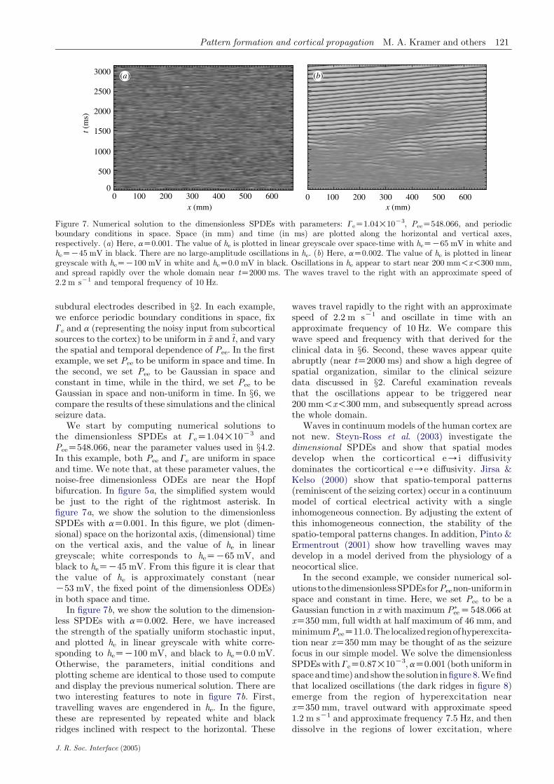
Figure 7. Numerical solution to the dimensionless SPDEs with parameters: GeZ1.04!10K3, PeeZ548.066, and periodicboundary conditions in space. Space (in mm) and time (in ms) are plotted along the horizontal and vertical axes,respectively. (a) Here, aZ0.001. The value of he is plotted in linear greyscale over space-time with heZK65 mV in white andheZK45 mV in black. There are no large-amplitude oscillations in he. (b) Here, aZ0.002. The value of he is plotted in lineargreyscale with heZK100 mV in white and heZ0.0 mV in black. Oscillations in he appear to start near 200 mm!x!300 mm,and spread rapidly over the whole domain near tZ2000 ms. The waves travel to the right with an approximate speed of2.2 m sK1 and temporal frequency of 10 Hz.


subdural electrodes described in §2. In each example,we enforce periodic boundary conditions in space, fixGe and a (representing the noisy input from subcorticalsources to the cortex) to be uniform in ~x and ~t, and varythe spatial and temporal dependence of Pee. In the firstexample, we set Pee to be uniform in space and time. Inthe second, we set Pee to be Gaussian in space andconstant in time, while in the third, we set Pee to beGaussian in space and non-uniform in time. In §6, wecompare the results of these simulations and the clinicalseizure data.

We start by computing numerical solutions tothe dimensionless SPDEs at GeZ1.04!10K3 andPeeZ548.066, near the parameter values used in §4.2.In this example, both Pee and Ge are uniform in spaceand time. We note that, at these parameter values, thenoise-free dimensionless ODEs are near the Hopfbifurcation. In figure 5a, the simplified system wouldbe just to the right of the rightmost asterisk. Infigure 7a, we show the solution to the dimensionlessSPDEs with aZ0.001. In this figure, we plot (dimen-sional) space on the horizontal axis, (dimensional) timeon the vertical axis, and the value of he in lineargreyscale; white corresponds to heZK65 mV, andblack to heZK45 mV. From this figure it is clear thatthe value of he is approximately constant (nearK53 mV, the fixed point of the dimensionless ODEs)in both space and time.

In figure 7b, we show the solution to the dimension-less SPDEs with aZ0.002. Here, we have increasedthe strength of the spatially uniform stochastic input,and plotted he in linear greyscale with white corre-sponding to heZK100 mV, and black to heZ0.0 mV.Otherwise, the parameters, initial conditions andplotting scheme are identical to those used to computeand display the previous numerical solution. There aretwo interesting features to note in figure 7b. First,travelling waves are engendered in he. In the figure,these are represented by repeated white and blackridges inclined with respect to the horizontal. These


waves travel rapidly to the right with an approximatespeed of 2.2 m sK1 and oscillate in time with anapproximate frequency of 10 Hz. We compare thiswave speed and frequency with that derived for theclinical data in §6. Second, these waves appear quiteabruptly (near tZ2000 ms) and show a high degree ofspatial organization, similar to the clinical seizuredata discussed in §2. Careful examination revealsthat the oscillations appear to be triggered near200 mm!x!300 mm, and subsequently spread acrossthe whole domain.

Waves in continuum models of the human cortex arenot new. Steyn-Ross et al. (2003) investigate thedimensional SPDEs and show that spatial modesdevelop when the corticortical e/i diffusivitydominates the corticortical e/e diffusivity. Jirsa &Kelso (2000) show that spatio-temporal patterns(reminiscent of the seizing cortex) occur in a continuummodel of cortical electrical activity with a singleinhomogeneous connection. By adjusting the extent ofthis inhomogeneous connection, the stability of thespatio-temporal patterns changes. In addition, Pinto &Ermentrout (2001) show how travelling waves maydevelop in a model derived from the physiology of aneocortical slice.

In the second example, we consider numerical sol-utions to thedimensionlessSPDEsforPeenon-uniforminspace and constant in time. Here, we set Pee to be aGaussian function in x with maximum P�

eeZ548:066 atxZ350 mm, full width at half maximum of 46 mm, andminimumPeeZ11.0.The localizedregionofhyperexcita-tion near xZ350 mm may be thought of as the seizurefocus in our simple model. We solve the dimensionlessSPDEswithGeZ0.87!10K3,aZ0.001 (both uniform inspace and time) and showthe solution infigure 8.Wefindthat localized oscillations (the dark ridges in figure 8)emerge from the region of hyperexcitation nearxZ350 mm, travel outward with approximate speed1.2 m sK1 and approximate frequency 7.5 Hz, and thendissolve in the regions of lower excitation, where

0

500

1000

1500

2000

2500

3000

100 200 300x (mm)

t (m

s)

400 500 600

Figure 8. Numerical solution to the dimensionless SPDEs withparameters: GeZ0.87!10K3, aZ0.001, Pee a Gaussian func-tion in space with maximum 548.066 at xZ350 mm and fullwidth at half maximum 46 mm, and periodic boundaryconditions in space. Space (in mm) and time (in ms) areplotted along the horizontal and vertical axes, respectively.Thevalue ofhe is plotted in linear greyscalewithheZK100 mVin white and heZ0.0 mV in black. Waves in he travel outwardfrom the region of hyperexcitation near xZ 350 mm withapproximate speed 1.2 m sK1 and approximate frequency7.5 Hz.


Pee/11.0. This localized oscillatory activity is morerepresentative of a localized seizure than the globaloscillations illustrated in figure 7b.

In the final example, we compute numerical solutionsto the dimensionless SPDEs for Pee non-uniform inspace and time. As in the previous example, we fixGeZ0.87!10K3andaZ0.001(bothuniforminspaceandtime).However,unlikethepreviousexample,wevaryPee

in time. At tZ{0, 5000} ms, we fix PeeZ11.0 uniform inspace. For 500 ms!t!5000 ms, we set Pee to bea Gaussian function in x with maximum P�

ee atxZ350 mm, full width at half maximum of 46 mm, andminimum Pee/11.0. At tZ{500, 1000, 1500, 2000,2500} ms, we increase P�

ee in steps of 100 so thatP�eeZf110; 210; 310; 410; 510g, respectively. These

increases are marked by the solid vertical lines infigure 9a. We then decrease P�

ee in steps of100 so that for tZ{3000, 3500, 4000, 4500} ms,P�eeZf410; 310; 210; 110g, respectively. These decreases

are marked by the dashed lines in figure 9b. We show infigure 9 that localized oscillations in he (the dark ridges)begin at tZ1900 ms, where P�

eeZ310. The frequency ofthese oscillations increaseswhenwe increaseP�

ee to 510attZ2500 ms. Then, as we decrease P�

ee between3000 ms!t!5000 ms, the oscillations in he decrease infrequency and eventually disappear.

This simple example provides a crude model for theevolution of the seizing cortex. At normal levels ofsubcortical excitation (PeeZ11.0) there exist onlydisorganized spatio-temporal fluctuations in he and nopathological oscillatory activity. Only when P�

ee exceedsa threshold level do localized oscillations in he appear.As the subcortical excitation is increased further, the


frequency of the oscillations increases. Then, as P�ee is

decreased, the oscillations slow and eventuallydisappear.

6. RESULTS

In §2, we showed ECoG data recorded at twoneighbouring electrodes during seizure, and in §§3–5,we computed numerical solutions to a continuummodelof cortical electrical activity. Here, we compare theobserved ECoG data with the model solutions for he.Specifically, we compute two quantities: (i) the averagefrequency at which the power spectrum achieves itsmaximum during seizure, and (ii) the average speed atwhich the voltage peaks propagate between twosubdural electrodes during seizure. We denote thesequantities f0 (the peak frequency) and v (the propa-gation speed), respectively. We show that f0 and v,computed from the model solutions and the ECoGseizure data, are roughly in agreement.

In our determination of f0, we consider data collectedat the same two subdural electrodes (e.g. X and Y ) foreach of six seizures from the same patient. Part of onesuch seizure is shown in figure 1. To compute f0, we firstlow pass filter the ECoG dataX andY below 55 Hz, andthen compute the WPS. For example, in figure 2a weshow the WPS for the time-series X recorded during atypical seizure. In this case, the maximum power occursbetween 1 and 10 Hz following seizure onset (attz17.5 s). To determine f0, we calculate the averagefrequency of maximum power in the WPS for theduration of the seizure (here, for 17.5 s!t!50 s). Welist f0 and its standard deviation over the duration of theseizure for both electrodes (i.e. X and Y ) and eachseizure in table 3. For reference, we label the seizures S1to S6, where S1 corresponds to the data discussed in §2.We also compute the average of f0 over the six seizuresforX andY and find 4.1G0.8 and 5G1 Hz, respectively.

Propagating waves of electrical activity have beenobserved in numerous mammalian systems and duringseizures in rats and in cats (Chervin et al. 1988; Connors& Amitai 1993; Pinto & Ermentrout 2001). Here, weassume that, during each seizure, voltage peaks propa-gate between the two neighbouring subdural electrodes(with time-series X and Y ). That this assumption isvalid can be inferred from the data shown in figure 1b.We note for 17.5 s!t!27 s the similarity of the waveforms inX andY and that peaks inX precede peaks inY.To determine the average propagation speed v of thesevoltage peaks, we first low pass filter the time-seriesbelow 55 Hz.We then compute theWCCbetweenX andY, as shown in figure 3 for S1. At each time in theWCC, amaximum correlation occurs for some lag time. Forexample, at tZ20 s, the maximum correlation occurs ata lag of approximately 25 ms. We compute this lag atwhich the maximum correlation occurs for the durationof the seizure.We find that, in general, the lag values areconsistent over two temporal intervals.Thefirst interval(I1) includes the time of seizure onset and the 10 s thatfollow. The second interval (I 2) includes all later times(i.e. all times 10 s after the seizure onset until seizuretermination). For example, in S1 the two time-intervalsover which the lag of maximum correlation is consistentare: I 1Z17.5 s!t!27 s and I 2Z28 s!t!50 s. Such

Table 3. The peak frequency f0 for the ECoG time-series data recorded at electrodes X (first row) and Y (second row) for each ofsix seizures and the average over the six seizures.(For each seizure, we write the mean and the standard deviation of the mean. To compute the uncertainty in the average, weassume the uncertainties in f0 for each seizure are independent and random and propagate the uncertainties in the standard way.)

seizure label S1 S2 S3 S4 S5 S6 average

f0 of X (Hz) 3.9G0.2 3.6G0.2 3.1G0.3 4.3G0.3 4.3G0.3 5.4G0.6 4.1G0.8f0 of Y (Hz) 5.1G0.5 3.8G0.3 3.9G0.3 4.6G0.4 5.3G0.4 6.2G0.5 5G1

Table 4. The speed v at which excitation propagates during two time-intervals I 1 (immediately following seizure onset) and I 2(the later portion of the seizure) for each of six seizures.(The averages are computed in interval I 1 using seizures S1 to S5, and in interval I 2 using seizures S1, S2, S4 and S5. For eachseizure, we write the mean and the standard deviation of the mean. To compute the uncertainty in the average, we assume theuncertainties in v for each seizure are independent and random and propagate the uncertainties in the standard way.)

seizure label S1 S2 S3 S4 S5 S6 average

v in I 1 (m sK1) 0.42G0.02 0.49G0.03 0.75G0.06 0.45G0.02 0.63G0.7 — 0.5G0.1v in I 2 (m sK1) K2.6G0.2 K5G1 N K4.3G0.8 0.51G0.03 — K3G1

3000

x (m

m)

3500 4000

t (ms)t (ms)

4500 5000250020001500100050000

100

200

300

400

500

600

(a) (b)

Figure 9. Numerical solution to the dimensionless SPDEs with parameters GeZ0.87!10K3, aZ0.001, and periodic boundaryconditions in space. At tZ{0, 5000},PeeZ11.0 uniform in space. For 500 ms!t!5000 msPee is a Gaussian function in space withmaximum P�

ee at xZ350 mm and full width at half maximum 46 mm. In subfigure (a), the maximum P�eeZf110:0; 210:0; 310:0;

410:0; 510:0g at tZ{500, 1000, 1500, 2000, 2500} ms, respectively. These increases in P�ee are denoted by the solid vertical lines. In

subfigure (b), the maximum P�eeZf410:0; 310:0; 210:0; 110:0g at tZ{3000, 3500, 4000, 4500} ms, respectively. These decreases in

P�ee are denoted by the dashed vertical lines. Space (in mm) and time (in ms) are plotted along the vertical and horizontal axes,

respectively. The value of he is plotted in linear greyscale with heZK100 mV in white and heZ0.0 mV in black. Waves in he arelocalized in space and time to the region of hyperexcitation near xZ350 mm for 1800 ms!t!3800 ms.


intervals can be chosen for each seizure except S6. Forthis seizure, the lag values of maximum correlation arenear zero for all times following seizure onset. Therefore,we do not include S6 in our analysis of v. We determine vin each interval by dividing the known electrodeseparation (10 mm) by the average lag in each interval.We list v and its standard deviation in each interval andfor each seizure in table 4. We note that for S3 theaverage lag is 0 ms in I 2 and therefore v is infinite. Wecompute the average and standard deviations of v in I 1(over S1 to S5) and I 2 (over S1, S2, S4 and S5) to find0.5G0.1 and K3G1 m sK1, respectively. We note thattravelling waves of electrical activity on animal corticeshave been reported with speeds of 0.06–0.09 m sK1

(Chervin et al. 1988).


To compare these observational results with themodel results, we compute f0 and v from the numericalsolutions to the model cortex for the variable he.We tabulate the results in table 5 for the dimensionlessODEs simulation shown in figure 5a, and the dimen-sionless SPDEs simulations shown in figures 7b and 8.We note that the results of the simulations agree withthe observed data for f0 (within a factor of 2) and v in I 1(within a factor of 5).

7. DISCUSSION

Our aim was to consider the potential of the SPDEsto provide a model of the mesoscopic electrical activityon the seizing cortex. In our analysis of the dimensionless

Table 5. The peak frequency f0 and wave speed v determinedfor the model solutions of he.

simulation f0 (Hz) v

ODE (figure 5b) 7.5 —PDE (figure 7b) 10.0 2.2 m sK1

PDE (figure 8) 7.5 1.2 m sK1


ODEs, we have shown that there do exist limit cycles inhe associated with Hopf bifurcations in the dynamics.We have also shown that the simpler dimensionlessODEs suggest behaviour in the complicated dimension-less SPDEs that is consistent with the clinical seizuredata. Specifically, we have shown that at typicalparameter values GeZ1.42!10K3 and PeeZ11.0, areduction in Ge (to GeZ1.20!10K3) produced oscil-latory behaviour in he. However, this oscillatorybehaviour was transient and did not produce the large-amplitude, stable oscillations characteristic of theseizing cortex. Moreover, this oscillatory behaviouroccurred at a single value of Ge. Thus, the parametervalues of the model cortex would have to be carefullytuned to reach this point.

To increase the excitability of the model cortex andmake it ‘seize’, we increased Pee. We show in figures 5aand 6 that for PeeO250.0 there exist stable, large-amplitude limit cycles in he over a wide range of Ge. Wesuggest in §5 that these oscillations are associated withtravelling wave dynamics in the dimensionless SPDEs.Thus to produce behaviour in he consistent with thatobserved in the seizing cortex, we must: (i) increase Pee,and (ii) decrease Ge in the dimensionless SPDEs. Indimensional terms, we must increase the subcorticalexcitation pee or decrease the maximum firing rateSmax, and we must increase the EPSP neurotransmitterrate constant ge or the difference between the reversaland resting potentials jhreve Khrestj or decrease the peakexcitatory postsynaptic potential Ge or S

max.That we must decrease Ge to induce a seizure seems

counterintuitive. We expect that an increase in thestrength of excitatory inputs would promote seizingactivity. However, the decrease in Ge, from 1.42!10K3

to 0.87!10K3 used to create figure 9, represents only a39% change. The change in Pee required to induce aseizure is much larger. We show in figure 9 that thisparameter must increase by at least 2700%. We mayinterpret the changes in these two parameters requiredfor seizure induction following the models in da Silvaet al. (2003). Alterations of the epileptic brain, owing togenetic or environmental (e.g. injury) effects, forexample, predispose it to seizures. In modelling theepileptic cortex, we may interpret this predisposition asa permanent (model I) or a gradual (model II or modelIII) change of a model parameter. The results shown infigure 9 illustrate the latter case; with Ge fixed, agradual increase in Pee induces seizing activity in he.Because the change in Pee is gradual and affects thedynamics of he we could try to anticipate these types ofseizures. We may also interpret these results followingthe model I framework. For example, consider apermanent increase in Pee from 11.0 to 310.0. When


modelling the cortical activity of any individual (eitherhealthy or epileptic), we may assume that the modelparameters undergo routine fluctuations in theirnormal values. In healthy individuals (with the typicalparameter value PeeZ11.0), a small negative fluctu-ation in the model parameter Ge may induce a harmless,transient oscillation (like that shown in figure 4) butnot a seizure. This same fluctuation in Ge will causethe predisposed epileptic cortex to seize. In this case,the increased value of Pee allows the dynamics to crossthe separatrix (or boundary) between the normal andseizing states (Robinson et al. 2002). Thus, only a smallchange in Ge is necessary to produce pathologicaloscillations in he. Because a random fluctuation inGe induces the seizure, these types of seizures cannot beanticipated. From the results presented here, wesuggest a large change in Pee and a small change inGe may provide a model of the seizing cortex.

In tables 3–5 we compute two results, the averagepeak frequency f0 and the average propagation speed v,derived from clinical ECoG recordings and solutions tothe SPDEs. We find that the values derived from theobservational and model data approximately agree(f0 within a factor of 2 and v in I 1 within a factor of 5),but note the following important issues. First, thesubdural electrode strips used in the clinical recordingsconsist of six electrodes each separated by 10 mm.Thus, the spatial sampling of the cortex is poor and wecannot observe detailed wave behaviour in the voltage.It may be true that electrodes X and Y lie on eitherside of a sulcus (a groove or furrow in the cortex); theprecise locations are not known. It may also be truethat a wave in electrical potential is propagatingobliquely with respect to the shortest path betweenelectrodes X and Y. Future recordings that utilizehigh-density electrode grids with small interelectrodespacing would provide better results to compare withthe theory. Second, the lead/lag relationships deter-mined from the WCC are ambiguous. For example, weshowed in figure 3 that for 17.5 s!t!27 s, theoscillations at electrode X lead the oscillations atelectrode Y by approximately 25 ms. During thisinterval, these time-series are nearly sinusoidal witha well-defined frequency near 4 Hz; see the data infigure 1b or the WPS in figure 2. The cross-correlationof two sinusoids is itself a sinusoid, and thereforeambiguous; although we suggest X leads Y byapproximately 25 ms, it is also true that Y leadsX by approximately 225 ms (the period of the 4 Hzcycle minus 25 ms). We chose the case X leads Y fortwo reasons: (i) the amplitude of oscillations in X isbigger than in Y, and (ii) a correlation at 25 msbetween two closely spaced electrodes is more reason-able than a correlation of 225 ms. It does not seempossible to resolve this ambiguity of the cross-correlation. Third, we have assumed that the samevoltage wavefront passes through both electrodes. Ifthe wave source lies between the two electrodes, thenthis assumption is incorrect. Smaller electrode spacingmay help locate the wave source more accurately.Fourth, given such a complicated model (14 nonlinearfirst-order stochastic differential equations and 20parameters), we could potentially produce any desired


behaviour in he by properly tuning the parameters.Here, we chose to adjust two parameters, both relatedto the excitation of the model cortex. In this way, weused the physiology of the seizing cortex to constrainthe adjustable parameters in the model. Finally, we donot mean to suggest that the SPDEs provide anaccurate model of all human cortical seizure activity.Here, we have only compared the model results withdata collected from a single subject, and shown thatthe model and observational data agree in anapproximate way.

Although confounding factors exist both in themodel and observations, these results still illustratean important use of the SPDEs and other continuummodels: establishing links between the known ECoGdata and unknown cortical physiology. Traditionally,neurophysiologists visually analyse ECoG datarecorded from a seizing patient. No attempt is madeto link the changes observed in these time-series withcorresponding changes in cortical physiology. Conti-nuum models of cortical electrical activity allow one toconsider such links in a quantitative way. This isespecially important for human cortical data, whereinvasive procedures are inappropriate. For example,Robinson et al. (2002) consider an ODE model of thecorticothalamic network. Unlike the SPDEs modelpresented here, these models explicitly include theinteractions of cortical neurons with the thalamus. Theauthors show that the model can produce the 3 Hz spikewave characteristic of absence seizures and how themodel parameters relate to the period of the seizures. Acorticothalamic model is used to study other types ofepilepsy in da Silva et al. (2003). In this work, we relatethe emergence of pathological oscillations in themeasured cortical voltage to changes in two par-ameters: a small decrease in Ge and a large increase inPee. In this way, we suggest a link between the ECoGdata and the physiology of the cortex.

Measures of dynamical quantities may also becomputed from observed and simulated time-seriesand compared. For example, the correlation dimension,largest Lyapunov exponent (LLE), and synchroniza-tion have been shown in observations to decreasepreceding a seizure (Quyen et al. 2003; Iasemidis 2003).Such quantities are calculable from the modelequations. Dafilis et al. (2001) vary two dimensionalparameters (pee and pei) and compute the LLE andKaplan–Yorke dimension for the dimensional ODEsmodel from Liley et al. (1999). A similar analysis maybe performed in which one varies the parameters Pee

and Ge of the dimensionless ODEs model presentedhere. Although the dimension and LLE determinedfrom noisy ECoG data are of limited accuracy, acomparison of the theoretical and observational resultsmay provide verification or suggest improvements tothe model (Freeman 1992).

Understanding both the ECoG patterns of corticalictal activity and the related changes in corticalphysiology may help shape new strategies for seizuredetection and focus location. This, in turn, may allowclinicians to deliver abortive seizure therapy that istargeted both in time and in space. For example,experimental methods such as focal cooling, brief pulse


cortical electrical stimulation and local drug delivery alldepend on reliable algorithms for the detection andprediction of seizures (Eder et al. 1997; Lesser et al.1999; Yang et al. 2002). The combination of parametersone can change in a well-motivated, physiologicallyrelevant model to simulate these dynamics may suggeststrategies for therapeutic intervention.

APPENDIX A.

Here, we non-dimensionalize the SPDEs fromSteyn-Ross et al. (2003). To do so we replace eachdynamical variable, as well as space x and time t, withits dimensionless counterpart. For example, we replacehe (the population mean soma voltage in Steyn-Rosset al. 2003) with h0e ~he, where h

0eZhreste ZK70 mV and ~he

is dimensionless. The main advantage of recastingthe equations in dimensionless form is a reduction in thenumber of parameters. There are 20 parameters inthe dimensionless SPDEs; in the original SPDEs thereare 29. We find for the dimensionless SPDEs:

v~hev~t

Z1K~heCGeðh0eK~heÞ~I eeCGiðh0i K~heÞ~I ie; (A1a)

v~hiv~t

Z1K~hiCGeðh0eK~hiÞ~I eiCGiðh0i K~hiÞ~I ii; (A1b)

1

Te

v

v~tC1

� �2

~I eeZNbe~Se½~he�C~feCPeeC~G1; (A1c)

1

Te

v

v~tC1

� �2

~I eiZNbe~Se½~he�C~fiCPeiC~G2; (A1d)

1

Ti

v

v~tC1

� �2

~I ieZNbi~S i½~hi�CPieC~G3; (A1e)

1

Ti

v

v~tC1

� �2

~I iiZNbi~S i½~hi�CPiiC~G4; (A1f )

1

le

v

v~tC1

� �2

~feZ1

l2e

v2~fe

v~x2

C1

le

v

v~tC1

� �Na

e~Se½~he�; (A1g)

1

li

v

v~tC1

� �2

~fiZ1

l2i

v2~fi

v~x2

C1

li

v

v~tC1

� �Na

i~Se½~he�: (A1h)

The eight dynamical variables in this system (~he, ~hi,~I ee, ~I ei, ~I ie, ~I ii, ~fe and ~fi) are functions of dimensionlessspace and time, ~x and ~t, respectively. We illustrate theconnections between these dynamical variables infigure 10. The dimensionless variables and parametersare defined in tables 1 and 2, respectively. Eachvariable and parameter is expressed in terms of itsdimensional counterparts from Steyn-Ross et al.(2003). In these tables, we have made the notationalsimplifications in agreement with the values used inSteyn-Ross et al. (2003): teZtiZt, Smax

e ZSmaxi ZSmax

and hreste Zhresti Zhrest. The dynamical variable heZh0e ~heis the key observable and related to the scalp EEGorECoG signal (Liley et al. 2002).

he hi

Iee Iei Iie

fe

fi

Pee Pei Pie Pii

Iii

Figure 10. A schematic of the eight dynamical variables(boxed) and the four subcortical inputs (Pee, Pei, Pie, Pii). Thevariables are defined in table 1; they appear in the dynamicalequations (A 1a–h). We indicate the interactions between thevariables using arrows. A schematic of the cortical macro-column may be found in fig. 2 of Liley et al. (1999).


We also define the dimensionless sigmoid transferfunctions:

~Se½~he�Z1

1Cexp½K~geð~he K ~qeÞ�; (A 2a)

~S i½~hi�Z1

1Cexp½K~gið~hi K ~qiÞ�; (A 2b)

and the dimensionless stochastic input terms:

~G1 Zaee

ffiffiffiffiffiffiffiPee

px1½~x; ~t� (A 3a)

~G2 Zaei

ffiffiffiffiffiffiPei

px2½~x; ~t� (A 3b)

~G3 Zaie

ffiffiffiffiffiffiPie

px3½~x; ~t� (A 3c)

~G4 Zaii

ffiffiffiffiffiffiPii

px4½~x; ~t�: (A 3d)

The terms in equations (A 3a–d ) represent the noisethat arises from subcortical inputs to the cortex. Here,the xk are Gaussian distributed white noise sources withzero mean and d-function correlations. In numericalsimulations, the xk are approximated as

xk½~x; ~t�ZRðm;nÞffiffiffiffiffiffiffiffiffiffiffiD~xD~t

p ; (A 4)

where ~xZmD~x and ~tZnD~t, (m, n integers), specifyspace and time coordinates on a lattice with (dimen-sionless) grid spacings, D~x and D~t, respectively. Here,we set aeeZaeiZaieZaiiZa as in the stochasticsimulations of the spatio-adiabatic one-dimensionalcortex in Steyn-Ross et al. (2003).

M.A.K. would like to acknowledge the support of a GraduateFellowship from the U.S. National Science Foundation, and aBerkeley Fellowship from the University of California. Theauthors are grateful to Nicholas M. Barbaro, MD, forelectrode placement and surgical management.


REFERENCES

Chervin, R. D., Pierce, P. A. & Connors, B. W. 1988Periodicity and directionality in the propagation ofepileptiform discharges across neocortex. J. Neurophysiol.60, 1695–1713.

Connors, B. W. & Amitai, Y. 1993 Generation of eliptiformdischarge by local circuits of neurocortex.. In Epilepsy:models,mechanisms,andconcepts (ed.P.A.Schwartkroin),pp. 388-423. Cambridge: Cambridge University Press.

Dafilis, M. P., Liley, D. T. J. & Cadusch, P. J. 2001 Robustchaos in a model of the electroencephalogram: implicationsfor brain dynamics. Chaos 11, 474–478.

da Silva, F. L., Blanes, W., Kalitzin, S. N., Parra, J.,Suffczynski, P. & Velis, D. N. 2003 Epilepsies as dyna-mical diseases of brain systems: basic models of the tran-sition between normal and epileptic activity. Epilepsia 44,72–83.

Dichter, M. A. & Ayala, G. F. 1987 Cellular mechanisms ofepilepsy: a status report. Science 237, 157–164.

Doedel, E., Paffenroth, R., Champneys, A., Fairgrieve, T.,Kuznetsov, Y. A., Sandstede, B. & Wang, X. 2000 AUTO

2000: continuation and bifurcation software for ordinarydifferential equations (with homcont. See http://source-forge.net/projects/auto2000/.

Ebersole, J. S. & Pacia, S. V. 1996 Localization of temporallobe foci by ictal eeg patterns. Epilepsia 37, 386–399.

Eder, H. G., Stein, A. & Fisher, R. S. 1997 Interictal and ictalactivity in the rat cobalt/pilocarpine model of epilepsydecreased by local perfusion of diazepam. Epilepsy Res.29, 17–24.

Freeman, W. J. 1964 A linear distributed feedback model forprepyriform cortex. Exp. Neurol. 10, 525–547.

Freeman, W. J. 1992 Tutorial in neurobiology: from singleneurons to brain chaos. Int. J. Bifurcat. Chaos 2, 451–482.

Higham, D. J. 2001 An algorithmic introduction to numericalsimulation of stochastic differential equations. SIAM Rev.43, 525–546.

Iasemidis, L. D. 2003 Epileptic seizure prediction and control.IEEE Trans. Biomed. Eng. 50, 549–558.

Jirsa, V. K. & Kelso, J. A. S. 2000 Spatiotemporal patternformation in neural systems with heterogeneous connec-tion topologies. Phys. Rev. E 62, 8462–8465.

Kramer, M. A. 2005 Nonlinear dynamics and neural systems:synchronization and modeling. PhD dissertation,University of California, Berkeley.

Lesser, R. P., Kim, S. H., Beyderman, L., Miglioretti, D. L.,Webber, W. R. S., Bare, M., Cysyk, B., Krauss, G. &Gordon, B. 1999 Brief bursts of pulse stimulationterminate afterdischarges caused by cortical stimulation.Neurology 53, 2073–2081.

Liley, D. T. J., Cadusch, P. J. & Wright, J. J. 1999A continuum theory of electro-cortical activity. Neuro-computing 26–27, 795–800.

Liley, D. T. J., Cadusch, P. J. & Dafilis, M. P. 2002A spatially continuous mean field theory of electrocorticalactivity. Network Comput. Neural Syst. 13, 67–113.

Morimoto, K., Fahnestock, M. & Racine, R. J. 2004 Kindlingand status epilepticus models of epilepsy: rewiring thebrain. Prog. Neurobiol. 73, 1–60.

Niedermeyer, E. & DaSilva, F. L. 1999 Electroencephalogra-phy: basic principles, clinical applications, and relatedfields. New York: Lippincott Williams and Wilkins.

Nunez, P. L. 1995 Neocortical dynamics and human EEGrhythms. New York: Oxford University Press.

Pinto, D. J. & Ermentrout, G. B. 2001 Spatially structuredactivity in synaptically coupled neuronal networks.I. Traveling fronts and pulses. SIAM J. Appl. Math.62, 206–225.

http://sourceforge.net/projects/auto2000/

http://sourceforge.net/projects/auto2000/


Quyen, M. L. V., Navarro, V., Martinerie, J., Baulac, M. &Varela, F. J. 2003 Toward a neurodynamical under-standing of ictogenesis. Epilepsia 44, 30–43.

Robinson, P. A., Rennie, C. J. & Rowe, D. L. 2002 Dynamicsof large-scale brain activity in normal arousal states andepileptic seizures. Phys. Rev. E 65, 041924.

Singer, W. 1993 Synchronization of cortical activity and itsputative role in information processing and learning.Annu. Rev. Physiol. 55, 349–374.

Singer, W. & Gray, C. M. 1995 Visual feature integration andthe temporal correlation hypothesis. Annu. Rev. Neurosci.18, 555–586.

Spencer, S. S., Guimaraes, P., Katz, A., Kim, J. & Spencer, D.1992 Morphological patterns of seizures recorded intracra-nially. Epilepsia 33, 537–545.

Steyn-Ross, M. L., Steyn-Ross, D. A., Sleigh, J. W. & Liley,D. T. J. 1999 Theoretical electroencephalogram stationaryspectrum for a white-noise-driven cortex: evidence for ageneral anesthetic-induced phase transition. Phys. Rev. E60, 7299–7311.

Steyn-Ross, M. L., Steyn-Ross, D. A., Sleigh, J. W. &Wilcocks, L. C. 2001a Toward a theory of the general-anesthetic-induced phase transition of the cerebralcortex. I. A thermodynamics analogy. Phys. Rev. E64, 011917.


Steyn-Ross, D. A., Steyn-Ross, M. L., Wilcocks, L. C. &Sleigh, J. W. 2001b Toward a theory of the general-anesthetic-induced phase transition of the cerebral cortex.II. Numerical simulations, spectral entropy, and corre-lation times. Phys. Rev. E 64, 011918.

Steyn-Ross, M. L., Steyn-Ross, D. A., Sleigh, J. W. &Whiting, D. R. 2003 Theoretical predictions for spatialcovariance of the electroencephalographic signal duringthe anesthetic-induced phase transition: increased corre-lation length and emergence of spatial self-organization.Phys. Rev. E 68, 021902.

Traub, R. D., Whittington, M. A., Buhl, E. H., LeBeau,A. B. F. E. N., Boyd, S., Cross, H. & Baldeweg, T. 2001A possible role for gap junctions in generation of very fasteeg oscillations preceding the onset of, and perhapsinitiating, seizures. Epilepsia 42, 153–170.

Wilson, H. R. & Cowan, J. D. 1972 Excitatory and inhibitoryinteractions in localized populations of model neurons.Biophys. J. 12, 1–24.

Wilson, H. R. & Cowan, J. D. 1973 A mathematical theory ofthe functional dynamics of cortical and thalamic nervoustissue. Kybernetik 13, 55–80.

Yang, X. F., Duffy, D. W., Morley, R. E. & Rothman, S. M.2002 Neocortical seizure termination by focal cooling:temperature dependence and automated seizure detection.Epilepsia 43, 240–245.

Pathological pattern formation and cortical propagation of epileptic seizures

Documents

Transcript of Pathological pattern formation and cortical propagation of epileptic seizures