REVIEW ARTICLEpublished: 03 December 2013doi: 10.3389/fphy.2013.00024

Robust stability at the Swallowtail singularityOleg N. Kirillov1* and Michael L. Overton2

1 Magneto-Hydrodynamics Division, Institute of Fluid Dynamics, Helmholtz-Zentrum Dresden-Rossendorf, Dresden, Germany2 Courant Institute of Mathematical Sciences, New York University, New York, NY, USA

Edited by:

Pantelis Damianou, University ofCyprus, Cyprus

Reviewed by:

Pantelis Damianou, University ofCyprus, CyprusPetre Birtea, West University ofTimisoara, Romania

*Correspondence:

Oleg N. Kirillov,Magneto-Hydrodynamics Division,Institute of Fluid Dynamics,Helmholtz-Zentrum Dresden-Rossendorf, PO Box 510119,D-01314 Dresden, Germanye-mail: o.kirillov@hzdr.de

Consider the set of monic fourth-order real polynomials transformed so that the constantterm is one. In the three-dimensional space of the coefficients describing this set,the domain of asymptotic stability is bounded by a surface with the Whitney umbrellasingularity. The maximum of the real parts of the roots of these polynomials is globallyminimized at the Swallowtail singular point of the discriminant surface of the setcorresponding to a negative real root of multiplicity four. Motivated by this example, wereview recent works on robust stability, abscissa optimization, heavily damped systems,dissipation-induced instabilities, and eigenvalue dynamics in order to point out someconnections that appear to be not widely known.

Keywords: abscissa, optimization, overdamping, asymptotic stability, Whitney umbrella, Swallowtail, caustic,

eigenvalue dynamics

1. INTRODUCTION. ZIEGLER-BOTTEMA DESTABILIZATIONPHENOMENON

In 1956, motivated by the paradoxical effect of dissipation on thethreshold of oscillatory instability of mechanical structures undernon-conservative loadings [1], Bottema [2] studied the domainof asymptotic stability1 of a fourth-order real polynomial

q(μ) = μ4 + b1μ3 + b2μ

2 + b3μ + b4. (1)

He observed that the necessary and sufficient conditions

b1 > 0, b2 > 0, b3 > 0, b4 > 0, b2 >b2

1b4 + b23

b1b3(2)

for the polynomial to be Hurwitz, i.e., to have all its roots inthe left half of the complex plane, are not changed by the trans-formation μ = cλ, where c = 4

√b4 > 0. Indeed, after denoting

ai = bic−i, i = 1, 2, 3, 4, (3)

the inequalities (2) are equivalent to the conditions

a1 > 0, a3 > 0, a2 > 2 + (a1 − a3)2

a1a3> 0 (4)

1An equilibrium of a dynamical system is said to be Lyapunov stable if allthe solutions starting in its vicinity remain in some neighborhood of theequilibrium in the course of time. For asymptotic stability, the solutions arerequired, additionally, to converge to the equilibrium as time tends to infin-ity. The first (indirect) method of Lyapunov reduces the study of asymptoticstability of an autonomous (time-independent) system to the problem of loca-tion in the complex plane of eigenvalues of the operator of its linearization.In a finite-dimensional case the eigenvalues are roots of a polynomial char-acteristic equation. Localization of all the roots in the open left half of thecomplex plane is a necessary and sufficient condition for asymptotic stabilityof a linearization, which usually implies asymptotic stability of the originalnon-linear system.

that are necessary and sufficient for the polynomial

p(λ) = λ4 + a1λ3 + a2λ

2 + a3λ + 1 (5)

to be Hurwitz. The domain (4) was plotted by Bottema in the(a1, a3, a2)-space; see Figure 1.

Bottema realized that the boundary � of the asymptotic sta-bility domain (4) is a ruled surface 2 generated by straight linesa3 = ra1, a2 = r + 1/r, where r ∈ (0, ∞). The boundary � has aself-intersection along the ray a2 ≥ 0 of the a2-axis. Two genera-tors pass through each point of the ray; they coincide at a2 = 2(r = 1), and for a2 → ∞ their directions tend to those of thea1- and a3-axis (r = 0, r = ∞). Remarkably [2, 3], the point(a1, a3, a2) = (0, 0, 2) is on �, but if one tends to the a2-axisalong the line a3 = ra1 the coordinate a2 has the limit r + 1/r > 2except for r = 1, when a2 = 2. The point (0, 0, 2) marked by thediamond symbol in Figure 1 is the Whitney umbrella singularity[4]. The surface defined by the equation

a2 = 2 + (a1 − a3)2

a1a3(6)

is just another representation of a standard crosscap surfacefstd(u, v) = (u, uv, v2) : R

2 → R3, which also bears the name of

the Whitney umbrella [5].For given a1 = a1,0 and a2 = a2,0 > 2, exactly two points cor-

respond at the crosscap (6) with the third coordinate determinedfrom the equation

a3,0 = 1

2

(a2,0 ±

√a2

2,0 − 4

)a1,0, (7)

2A surface is ruled if every one of its points lies on a line that belongs to thesurface; the ruled surface is literally swept out by these lines. Familiar examplesinclude a conical surface or a hyperboloid of one sheet.

www.frontiersin.org December 2013 | Volume 1 | Article 24 | 1

PHYSICS

Kirillov et al. Robust stability at the Swallowtail singularity

FIGURE 1 | A singular boundary � of the domain of asymptotic

stability (4) of the polynomial (5) with the Whitney umbrella

singularity at the point (a1, a3, a2) = (0, 0, 2), marked by the

diamond symbol. Inside the domain of asymptotic stability a part ofthe discriminant surface of the polynomial is situated with theSwallowtail singularity at the point (4, 4, 6) marked as an open circle.Inside the spike bounded by the discriminant surface all the roots ofthe polynomial (5) are real and negative. The green planar sector is thetangent cone (10) to the domain of asymptotic stability at the Whitneyumbrella singularity.

where each sign is associated with one of the two sheets of thecrosscap that intersect along the interval a2 ≥ 2; see Figure 1.Writing the equations for the tangent planes at these points

a1

(a2,0 ±

√a2

2,0 − 4

)− 2a3 =

a1,0

(a2,0 ±

√a2

2,0 − 4)2

a22,0 ± a2,0

√a2

2,0 − 4 − 4(a2 − a2,0)

(8)

we find that approaching the singular point (0, 0, 2) along thea2-axis, i.e., assuming a1,0 = 0 in (8) and then letting a2,0 tendto 2, results in the collapse of the two planes into one defined bythe equality

a1 = a3. (9)

The limit (9) of the tangent planes is the tangent cone to the cross-cap at the Whitney umbrella singularity [5]. A part of the plane(9) that lies inside the domain of asymptotic stability (4) consti-tutes a set of all directions leading from the point (0, 0, 2) to thestability region

{(a1, a3, a2) : a1 = a3, a1 > 0, a2 > 2} . (10)

The tangent cone (10) to the domain of asymptotic stability atthe Whitney umbrella singularity, which is shown in green inFigure 1, is degenerate in the (a1, a3, a2)-space because it selects a

set of measure zero on a unit sphere with the center at the singularpoint [6–8].

In 1971, Arnold [4] considered parametric families of realmatrices and studied which singularities on the boundary of theasymptotic stability domain in the space of parameters are notdestroyed by small perturbation of the family, i.e., are structurallystable or generic singularities. He composed a list of generic sin-gularities in parameter spaces of low dimension which revealed,in particular, that the Whitney umbrella persists on the stabilityboundary of a real matrix of arbitrary dimension if the num-ber of parameters is not less than three, i.e., the singularity is ofcodimension 3.

The singular point (a1, a3, a2) = (0, 0, 2) corresponds to adouble complex conjugate pair of roots λ = ±i of the polyno-mial (5).

At the line of self-intersection of the Whitney umbrella formedby the ray a2 > 2 of the a2-axis there are two distinct com-plex conjugate pairs of imaginary roots [2] indicating Lyapunov(marginal) stability. However, the threshold of stability a2 = 2 isextremely sensitive to the coefficients a1 and a3 as is seen from (6).

Indeed, fix a1 �= a2 and let a1 = εa1 and a3 = εa3 (where 0 <

ε � 1). Then, using (6), we find that the increment to the criticalvalue of the coefficient a2 is

�a2(ε) := a2 − 2 = (a1 − a3)2

a1a3∼ O(1). (11)

In other words, the stability threshold acquires a finite increment�a2 > 0 even if the perturbation of the coefficients a1 and a3 isinfinitesimally small for almost all combinations of a1 and a3,except in the case a1 = a3. The minimal threshold of marginalstability a2 = 2 at a1 = 0 and a3 = 0 corresponding to the doubleimaginary root is thus structurally unstable: generic combina-tions of the parameters a1 and a3 at a2 = 2 lie in the domain ofinstability [1–3, 9]. Therefore, looking for extremal values of aparameter (a2 in our case) at the boundary of asymptotic stabilitymay lead to structurally unstable stability thresholds at the sin-gular points of the stability boundary corresponding to multipleroots.

The more basic fact that multiple roots of a polynomialare sensitive to perturbation of the coefficients is a phe-nomenon that was studied already by Isaac Newton, whointroduced the so-called Newton polygon to determine theleading terms of the perturbed roots as fractional powers ofa perturbation parameter. It follows that, in matrix analy-sis, eigenvalues are in general not locally Lipschitz at pointsin matrix space with non-semi-simple eigenvalues3 [10–13],and, in the context of dissipatively perturbed Hamiltoniansystems, [9, 14, 15]. Thus, it has been well-understood fora long time that perturbation of multiple roots or multiple

3Those whose algebraic multiplicity exceeds their geometric multiplicity (thenumber of linearly independent associated eigenvectors) and that are there-fore associated with Jordan blocks of size 2 or higher in the Jordan canonicalform of the matrix.

Frontiers in Physics | Mathematical Physics December 2013 | Volume 1 | Article 24 | 2

Kirillov et al. Robust stability at the Swallowtail singularity

eigenvalues on or near the stability boundary is likely to lead toinstability4.

Because of the sensitivity of multiple roots and eigenvalues toperturbation, in engineering and control-theoretical applicationsa natural desire is to “cut the singularities off” by construct-ing convex inner approximations to the domain of asymptoticstability [17, 18]. Nevertheless, multiple roots per se are not unde-sirable. Indeed, multiple roots also occur deep inside the domainof asymptotic stability. Although it might seem paradoxical at firstsight, such configurations are actually obtained by minimizing theso-called polynomial abscissa in an effort to make the asymptoticstability of a linear system more robust, as we now explain.

2. ABSCISSA MINIMIZATION AND MULTIPLE ROOTSThe abscissa 5 of a polynomial p is the maximal real part of itsroots:

a(p) = max{Re λ : p(λ) = 0}. (12)

We restrict our attention to monic polynomials with real coeffi-cients and fixed degree n: since these have n free coefficients, thisspace is isomorphic to R

n. On this space, the abscissa is a continu-ous but non-smooth, in fact non-Lipschitz, as well as non-convex,function whose variational properties have been extensively stud-ied using non-smooth variational analysis [21–24].

Now set n = 4, consider the set of polynomials p(λ) defined in(5), and consider the restricted set of coefficients

{(a1, a3, a2) : a1 = a3, a2 = 2 + a2

1

4

}. (13)

For these coefficients, the abscissa a(p) is shown as a function ofa1 by the bold red curve in Figure 2. The roots are

λ1 = λ2 = −a1

4− 1

4

√a2

1 − 16, λ3 = λ4 = −a1

4+ 1

4

√a2

1 − 16.

(14)When 0 ≤ a1 < 4 (a1 > 4), the roots λ1,2 and λ3,4 are complex(real) with each pair being double, that is with multiplicity two. Ata1 = 4 there is a quadruple real eigenvalue −1. So, we refer to theset (13) as a set of exceptional points6 (abbreviated as the EP-set).

When a1 > 0, the EP-set (13) (shown by the red curve inFigure 3) lies within the tangent cone (10) to the domain ofasymptotic stability at the Whitney umbrella singularity (0, 0, 2).The points in the EP-set all define polynomials with two doubleroots (denoted EP2) except (a1, a3, a2) = (4, 4, 6), at which p hasa quadruple root and is denoted EP4; see Figure 3.

4In fact, even simple eigenvalues of non-Hermitian (more specifically, non-normal) matrices are often highly sensitive to perturbation, and when thisis the case, eigenvalues may not be a useful tool for studying system behav-ior, as they model only asymptotic behavior of linear systems, not transientor non-linear behavior. See [16] for further discussion of non-normalityand how alternatives to eigenvalues, notably pseudospectra, may be used tomodel physical systems; a particularly well-studied example is the transitionto turbulence in high Reynolds number fluid flows.5The contour plot of the abscissa in the plane of two parameters is known alsoas the decrement diagram [19, 20].6In the sense of T. Kato [15, 25, 26].

FIGURE 2 | The real parts of the roots of the polynomial (5) with the

coefficients in the set (13) and (shown by the bold red curve) the

abscissa (12).

FIGURE 3 | The discriminant surface (gray) and the tangent cone

(green) to the domain of asymptotic stability. Inside the tangent cone(10) the red curve marks the EP-set (13). The part of the EP-set above theSwallowtail singularity at the point (4, 4, 6) forms a line of self-intersectionof the discriminant surface. The bold black curves are cuspidal edges of thediscriminant surface corresponding to triple negative real roots.

Let us consider how the roots move in the complex planewhen a1 and a3 coincide and are set to specific values and a2

increases from zero, as shown by black curves in Figure 4. Whena1 = a3 < 4, the roots that initially have positive real parts andthus correspond to unstable solutions move along the unit cir-cle to the left, cross the imaginary axis at a2 = 2 and mergewith another complex conjugate pair of roots at a2 = 2 + a2

1/4,i.e., at the EP-set. Further increase in a2 leads to the splitting ofthe double eigenvalues, with one conjugate pair of roots mov-ing back toward the imaginary axis. By also considering the casea1 = a3 > 4, it is clear that when a1 and a3 coincide, the choicea2 = 2 + a2

1/4 minimizes the abscissa, with the polynomial p on

www.frontiersin.org December 2013 | Volume 1 | Article 24 | 3

Kirillov et al. Robust stability at the Swallowtail singularity

the EP-set, see Figure 5. Furthermore, when a1 = a3 is increasedtoward 4 from below, the coalescence points (EP2) move aroundthe unit circle to the left. This conjugate pair of coalescencepoints merges into the quadruple real root λ = −1 (EP4) whena1 = a3 = 4 and hence a2 = 6, as is visible in Figure 6. If a1 = a3

is increased above 4 the quadruple point EP4 splits again intotwo exceptional points EP2, one of them inside the unit circle,Figure 5.

Thus, all indications are that the abscissa is minimized by theparameters corresponding to EP4, with a quadruple root at −1. Infact, application of the following theorem shows that the abscissaof (5) is globally minimized by the EP4 parameters.

FIGURE 4 | Trajectories of roots of the polynomial (5) when a2

increases from 0 to 15 and: a1 = a3 = 3.7 (black); a1 = 3.7, a3 = 3.6

(red); a1 = 3.6, a3 = 3.7 (green).

FIGURE 5 | Trajectories of roots of the polynomial (5) when a2

increases from 0 to 15 and: a1 = a3 = 5 (black); a1 = 5, a3 ≈ 4.621 (red);

a1 ≈ 4.621, a3 = 5 (green), indicating that although three roots

coalesce into a triple negative real root (EP3) with Reλ < −1, there is

another simple negative real root with Reλ > −1.

Theorem [27, Theorems 7 and 14]7. Let F denote either the realfield R or the complex field C. Let b0, b1, . . . , bn ∈ F be given (withb1, . . . , bn not all zero) and consider the following family of monicpolynomials of degree n subject to a single affine constraint on thecoefficients:

P = {λn + a1λn − 1 + . . . + an − 1λ + an : b0

+n∑

j = 1

bjaj = 0, ai ∈ F}.

Define the optimization problem

a∗ := infp ∈ P

a(p). (15)

Let

h(λ) = bnλn + bn − 1

(n

n − 1

)λn − 1 + . . . + b1

(n

1

)λ + b0.

First, suppose F = R. Then, the optimization problem (15) has theinfimal value

a∗ = − max{ζ ∈ R : h(i)(ζ) = 0 for some i ∈ {0, . . . , k − 1}

},

where h(i) is the i-th derivative of h and k = max{j : bj �= 0}.Furthermore, the optimal value a∗ is attained by a minimizing poly-nomial p∗ if and only if −a∗ is a root of h (as opposed to one of itsderivatives), and in this case we can take

p∗(λ) = (λ − γ)n ∈ P, γ = a∗.

FIGURE 6 | Trajectories of roots of the polynomial (5) when a2

increases from 0 to 15 and: a1 = a3 = 4 (black); a1 = 4, a3 = 3.9 (red);

a1 = 3.9, a3 = 4 (green). The global minimum of the abscissa is attainedwhen all the roots coalesce into the quadruple root λ = −1 (EP4).

7As explained in [27], most of this result when F = R was established by R.Chen in a 1979 Ph.D. thesis.

Frontiers in Physics | Mathematical Physics December 2013 | Volume 1 | Article 24 | 4

Kirillov et al. Robust stability at the Swallowtail singularity

Second, suppose F = C. Then, the optimization problem (15)always has an optimal solution of the form

p∗(λ) = (λ − γ)n ∈ P, Re γ = a∗,

with −γ given by a root of h (not its derivatives) with largest realpart.

In our case, F = R, n = 4 and the affine constraint on thecoefficients of p is simply a4 = 1. So, the polynomial h is given by

h(λ) = λ4 − 1.

Its real root with largest real part is 1, and its derivatives haveonly the zero root. So, the infimum of the abscissa a over thepolynomials (5) is −1, and this is attained by

p∗(λ) = (λ + 1)4 = λ4 + 4λ3 + 6λ2 + 4λ + 1, (16)

that is, with the coefficients at the exceptional point EP4. There isnothing special about n = 4 here; if we replace 4 by n we find thatthe infimum is still −1 and is attained by p∗(λ) = (λ + 1)n.

3. SWALLOWTAIL SINGULARITY AS A GLOBAL MINIMIZEROF THE ABSCISSA

Let us look at the dynamics of the roots of the polynomial (5)in the complex plane, when a1 �= a3, i.e., when the variation ofa2 happens at a distance from the tangent cone (10). If a1 ≤ 4and a3 ≤ 4 (as in Figures 4, 6) the complex roots do not coa-lesce at EP2 or EP4 but instead some of them turn back towardthe imaginary axis before reaching the unit circle. Such parameterconfigurations are therefore not optimal. However, when a1 > 4or a3 > 4 other scenarios of the root movement are possible: forexample, formation of triple negative real roots as in Figure 5.Note, however, that even when the triple negative real root occursat Re λ < −1, there is another negative real root inside the unitcircle. Therefore, in accordance with the above Theorem, configu-rations with triple roots are not global minimizers of the abscissaof the polynomial (5). Nevertheless, it is instructive to understandthe set in the (a1, a3, a2)-space where the roots of the polynomialare real and negative, but not necessarily simple.

Consider the discriminant8 � of the polynomial (5) and equateit to zero:

� := 16a42 − 4(a2

1 + a23)a3

2 + (a21a2

3 − 80a1a3 − 128)a22

+ 18(a1a3 + 8)(a21 + a2

3)a2 + 256 − 27a43

− 27a41 − 6a2

1a23 − 192a1a3 − 4a3

1a33 = 0. (17)

In the (a1, a3, a2)-space, the polynomial (5) has at least one mul-tiple root at the points of the set given by (17). For example, inthe plane a1 = a3

� = (a2 + 2 + 2a3)(a2 + 2 − 2a3)(4a2 − 8 − a23)

2,

8The discriminant is a function of the coefficients of a polynomial which van-ishes if and only if the polynomial has a repeated (real or complex) root. Whenthe discriminant of a real polynomial changes its sign, a complex conjugatepair of roots either originates or disappears.

and the equation � = 0 yields the straight line a2 = 2(a3 − 1)

and parabola a2 = 2 + a23/4 that touch each other at a3 = 4 and

a2 = 6, which corresponds to the EP4 point in Figure 3. This cor-responds to the quadruple negative real root −1 of the polynomial(5), which is a global minimum of its abscissa.

Plotting the discriminant surface (17), we see in Figure 3 thatit has a self-intersection along the part of the EP-set (13) selectedby the inequality a2 ≥ 6 and two cuspidal edges defined in theparametric form as

a1 =a2

2 ± a2

√a2

2 − 36 − 12(a2 ±

√a2

2 − 36

)3/2

√6,

a3 =a2

2 ± a2

√a2

2 − 36 + 36

3

√6a2 ± 6

√a2

2 − 36

, a2 ≥ 6.

At the cuspidal edges the polynomial (5) has a triple negative realroot and a simple negative real root. For example, at the points(

289

√3, 4

√3, 10

)and

(4√

3, 289

√3, 10

)we have, respectively,

λ1 = −√

3

9, λ2, 3, 4 = −√

3, and

λ1 = −3√

3, λ2, 3, 4 = −√

3

3. (18)

At the point EP4 with the coordinates (4, 4, 6) in the (a1, a3, a2)-space the discriminant surface has the Swallowtail singularity,which is a generic singularity of bifurcation diagrams in three-parameter families of real matrices [19, 28]; see Figure 3.

Therefore, the coefficients of the globally minimizing poly-nomial (16) are exactly at the Swallowtail singularity of thediscriminant surface of the polynomial (5).

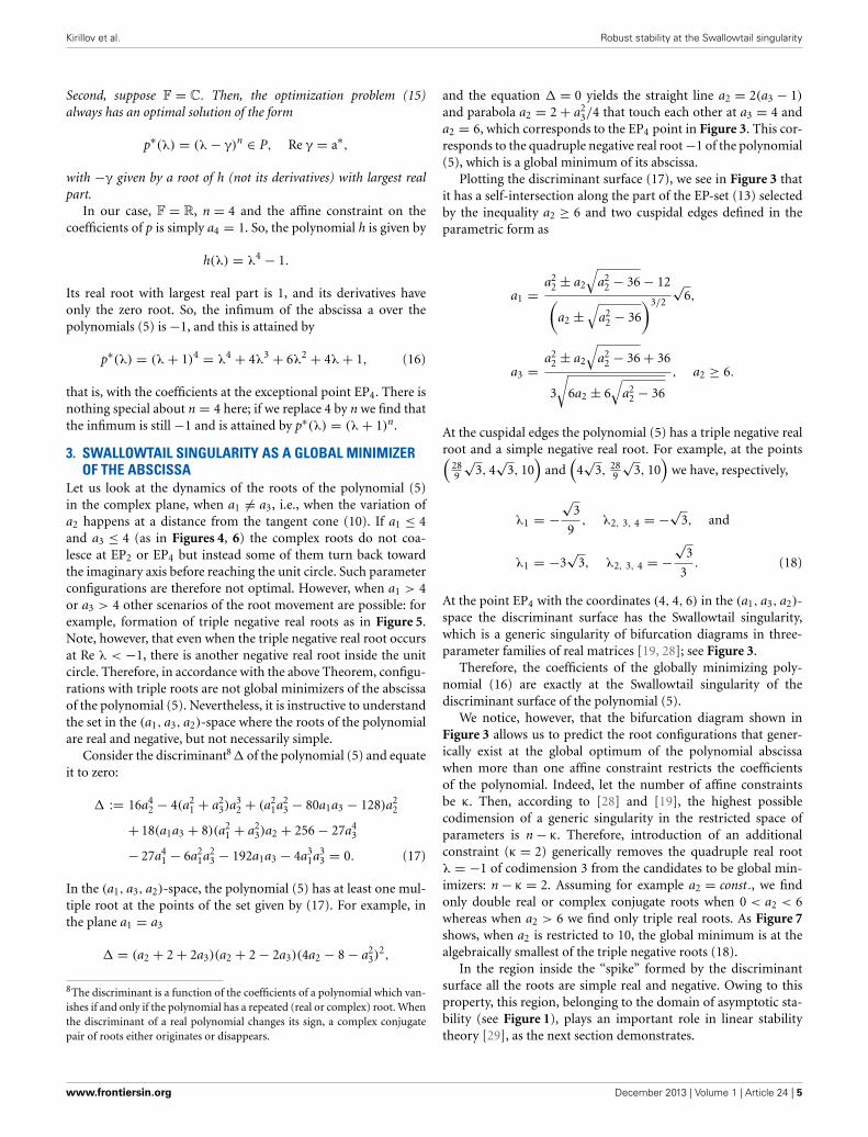
We notice, however, that the bifurcation diagram shown inFigure 3 allows us to predict the root configurations that gener-ically exist at the global optimum of the polynomial abscissawhen more than one affine constraint restricts the coefficientsof the polynomial. Indeed, let the number of affine constraintsbe κ. Then, according to [28] and [19], the highest possiblecodimension of a generic singularity in the restricted space ofparameters is n − κ. Therefore, introduction of an additionalconstraint (κ = 2) generically removes the quadruple real rootλ = −1 of codimension 3 from the candidates to be global min-imizers: n − κ = 2. Assuming for example a2 = const., we findonly double real or complex conjugate roots when 0 < a2 < 6whereas when a2 > 6 we find only triple real roots. As Figure 7shows, when a2 is restricted to 10, the global minimum is at thealgebraically smallest of the triple negative roots (18).

In the region inside the “spike” formed by the discriminantsurface all the roots are simple real and negative. Owing to thisproperty, this region, belonging to the domain of asymptotic sta-bility (see Figure 1), plays an important role in linear stabilitytheory [29], as the next section demonstrates.

www.frontiersin.org December 2013 | Volume 1 | Article 24 | 5

Kirillov et al. Robust stability at the Swallowtail singularity

FIGURE 7 | When a2 is restricted to 10, the abscissa of (5) reaches its

minimum at the triple negative real root −√

33

when a1 = 4√

3 and

a3 = 289

√3. The red curve is a cross-section of the discriminant surface (17)

by the plane a2 = 10.

4. HEAVILY DAMPED SYSTEMS IN MECHANICS ANDPHYSICS

Consider a linear mechanical system described by the equa-tion [29]

x + Dx + Kx = 0, (19)

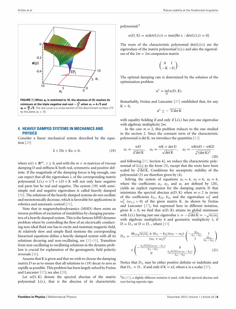
where x(t) ∈ IRm, t ≥ 0, and with the m × m matrices of viscousdamping D and stiffness K both real, symmetric and positive def-inite. If the magnitude of the damping forces is big enough, onecan expect that all the eigenvalues λ of the corresponding matrixpolynomial L(λ) = λ2I + λD + K will not only have negativereal parts but be real and negative. The system (19) with semi-simple real and negative eigenvalues is called heavily damped[30]. The solutions of the heavily damped systems do not oscillateand monotonically decrease, which is favorable for applications inrobotics and automatic control [31].

Note that in magnetohydrodynamics (MHD) there exists aninverse problem of excitation of instabilities by changing parame-ters of a heavily damped system. This is the famous MHD dynamoproblem where by controlling the flow of an electrically conduct-ing non-ideal fluid one has to excite and maintain magnetic field.At relatively slow and simple fluid motions the correspondinglinearized equations define a heavily damped system with all itssolutions decaying and non-oscillating, see [32–35]. Transitionfrom non-oscillating to oscillating solutions in the dynamo prob-lem is crucial for explanation of the geomagnetic field polarityreversals [36].

Assume that K is given and that we wish to choose the dampingmatrix D so as to ensure that all solutions to (19) decay to zero asrapidly as possible. This problem has been largely solved by Freitasand Lancaster [37]; see also [29].

Let α(D, K) denote the spectral abscissa of the matrixpolynomial L(λ), that is the abscissa of its characteristic

polynomial:9

α(D, K) = a(det(L(λ)) = max{Re λ : det(L(λ)) = 0}.

The roots of the characteristic polynomial det(L(λ)) are theeigenvalues of the matrix polynomial L(λ) and also the eigenval-ues of the 2m × 2m companion matrix

(0 I

−K −D

).

The optimal damping rate is determined by the solution of theoptimization problem

α∗ = infD

α(D, K).

Remarkably, Freitas and Lancaster [37] established that, for anyK > 0,

α∗ ≥ − 2m√

det K

with equality holding if and only if L(λ) has just one eigenvaluewith algebraic multiplicity 2m.

In the case m = 2, this problem reduces to the one studiedin the section 2. Since the constant term of the characteristicpolynomial is det K, we introduce the quantities [15]

a1 = trD4√

det K, a2 = trK + det D√

det K, a3 = trKtrD − trKD

4√

(det K)3

(20)and following [37, Section 4], we reduce the characteristic poly-nomial of L(λ) to the form (5), except that the roots have beenscaled by 4

√det K. Conditions for asymptotic stability of the

polynomial (5) are therefore given by (4).Solving the system of equations a1 = 4, a2 = 6, a3 = 4,

where the coefficients a1, a2, and a3 are defined by (20),yields an explicit expression for the damping matrix D thatminimizes the spectral abscissa α(D, K) when m = 2 in termsof the coefficients k11, k22, k12 and the eigenvalues ω2

1 andω2

2 (ω1,2 > 0) of the given matrix K. As shown by Freitasand Lancaster [37], but expressed here in different notation,given K > 0, we find that α(D, K) attains its global minimumwith L(λ) having just one eigenvalue λ = − 4

√det K = −√

ω1ω2

with algebraic multiplicity 4 and geometric multiplicity 1, ifD = D+ or D = D−, where [15]

D± = 4k12√

ω1ω2 ± (k11 − k22)(ω1 − ω2)

(ω1 + ω2)2

(− 2k12

k11 − k221

1 2k12k11 − k22

)

+(

− 4√

ω1ω2(ω1ω2 − k11)

k11 − k220

04√

ω1ω2(ω1ω2 − k22)

k11 − k22

). (21)

Notice that D± may be either positive definite or indefinite andthat D+ = D− if and only if K = κI, where κ is a scalar [37].

9In [37], a slightly different notation is used, with their spectral abscissa andours having opposite sign.

Frontiers in Physics | Mathematical Physics December 2013 | Volume 1 | Article 24 | 6

Kirillov et al. Robust stability at the Swallowtail singularity

Now we can give the following interpretation of the stabilitydiagram of Figure 1. The dissipative system (19) is asymptoti-cally stable inside the domain (4) with the coefficients a1, a2,and a3 defined by (20). The boundary of the domain (4) has theWhitney umbrella singular point at a1 = 0, a3 = 0, and a2 = 2.The domain corresponding to heavily damped systems of theform (19) is confined between three hypersurfaces of the discrim-inant surface (17) and has a form of a trihedral spike with theSwallowtail singularity at its cusp at a1 = 4, a2 = 6, and a3 = 4;see Figure 3. The Whitney umbrella and the Swallowtail sin-gular points are connected by the EP-set given by (13). At theSwallowtail singularity of the boundary of the domain of heav-ily damped systems, the abscissa of the characteristic polynomialof the damped potential system (19) attains its global minimum.

Therefore, by minimizing the spectral abscissa one finds pointsat the boundary of the domain of heavily damped systems.Furthermore, the sharpest singularity at this boundary corre-sponding to a quadruple real eigenvalue λ = − 4

√det K < 0 with

the Jordan block of order four is the very point where all themodes of the system (19) with m = 2 are decaying to zero asrapidly as possible when t → +∞.

5. DISCUSSIONTypical singularities of the contour plots of the abscissa (or decre-ment diagrams) in the plane of two parameters were listed alreadyby Arnold [19]. Let us have a closer look at the decrementdiagram of the polynomial (5) shown in Figure 8. The addi-tional constraint (a2 = 10) removes the quadruple real root fromthe generic singularities; hence, the minimizer of the abscissa is

the EP3 point corresponding to the triple root λ = −√

33 (see

Figure 7, which shows the graph of the abscissa in three dimen-sions). The lower (curved) contours in Figure 8 correspond to thereal parts of a complex-conjugate pair. The upper contours are

FIGURE 8 | The gray curves show the contour plot (decrement

diagram) of the abscissa a of the polynomial (5) when a2 is restricted

to 10. The green circle at the cusp of the red discriminant curve (17) marksthe location of the EP3 singularity, where the abscissa reaches its minimumin this case.

straight lines and correspond to a simple negative real root. Thecontours cross either at the points of the discriminant set (17)corresponding to the double negative real roots (the lower partof the red cuspidal curve in Figure 8) or at the points where bothcomplex conjugate roots and the real root have the same real part;see [19].

What are the relationships among the decrement diagram, sta-bility boundary, discriminant set, and abscissa minimization? Fora detailed answer it is simpler to consider a two-parameter cubicanalog of the polynomial family (5)

p(λ) := λ3 + a1λ2 + a2λ + 1 (22)

and to look closely not only at the active roots, that is those whosereal parts coincide with the abscissa a(p), but also at the remaininginactive roots, whose real part is algebraically smaller than a(p).

The polynomial (22) is Hurwitz if and only if

a1a2 > 1, a1 > 0, a2 > 0. (23)

The discriminant curve of the polynomial (22)

(a1a2 + 9)2 − 4(a31 + a3

2 + 27) = 0 (24)

bounds the domain of real roots in the (a1, a2) plane. It has a cuspsingularity at a1 = a2 = 3; see Figure 9. In accordance with the

FIGURE 9 | The green curves show the contour plot (decrement

diagram) of the abscissa a of the cubic polynomial (22) with contour

plots of the real parts of the inactive roots superimposed (red and gray

curves). The open circle marks the location of the EP3 singularity of thebifurcation diagram, where the abscissa reaches its minimum. Thecontours corresponding to simple real roots are straight lines that sweepout the cuspidal area confined between the boundaries of the bifurcationdiagram. In the limit, these contours are tangent to the black cuspidal curveand may be viewed as rays forming a caustic [19, 42, 44]. The curved greencontours correspond to real parts of a complex conjugate pair ofeigenvalues. The black hyperbola marks the stability boundary with thestable region above it and to the right. Along the stability boundary, a few(negative) gradient vectors of the real part of the complex conjugate pair ofactive eigenvalues are marked at a1 = 0.25, a1 = 1, and a1 = 4.

www.frontiersin.org December 2013 | Volume 1 | Article 24 | 7

Kirillov et al. Robust stability at the Swallowtail singularity

Theorem of section 2 the polynomial abscissa a(p) has its globalminimum at the singular EP3 point of the discriminant curvecorresponding to a triple root λ = −1.

Denotex = (a1, a2), y = Re(∇xλ), (25)

where the gradient of a root is given by the expression

∇xλ = −∇xp

∂λp. (26)

For example, taking into account that at the points of the stabilityboundary (a1a2 = 1) the roots are

λ1, 2 = ±i

√a1

a1, λ3 = −a1,

we find that the gradient of the real part of the complex-conjugatepair is

y(λ1, 2) = −1

2

(1

1 + a31

,a2

1

1 + a31

). (27)

Figure 9 is plotted in the (a1, a2) parameter space. The blackhyperbola shows the stability boundary, with the stable region(23) above and to the right. The small black strokes drawn atright angles to the hyperbola indicate some of the (negative)gradients (27).

The green curves and line segments in Figure 9 show the con-tours of the maximum of the real parts of the three roots of (22),i.e., they comprise a contour plot of the polynomial abscissa (thedecrement diagram). More specifically, the green curves in the sta-ble region correspond to a complex conjugate pair of active roots;in this region, as well as in the unstable region, the contours of theremaining inactive simple real root are shown by gray line seg-ments. The green line segments appearing in the top part of thefigure correspond to a simple real active root; in this region thecontours of the real part of the complex conjugate pair of inactiveroots are marked by the red curves.

Inside the cuspidal area whose boundary is exactly the discrim-inant curve given by (24), all three roots are real: the contours ofthe active root are marked by green segments, while the contoursof the two inactive real roots are shown by red and gray line seg-ments. In fact, the rays defined by the green, gray, and red linesegments shown in the figure sweep out the cuspidal area. Theboundary of the region of real roots can thus be viewed as a caus-tic or an evolute of the rays defining the contours of the negativereal roots [19]. The open circle at the cusp is the EP3 singularity,where the abscissa reaches its global minimum with all three rootsequal to −1.

10For example, movement of eigenvalues in parametric families of real sym-metric and Hermitian matrices possesses physical interpretation as dynamicsof Pechukas-Yukawa gas [45] which is an integrable multidimensional system;the latter fact in its turn is used for analysis and design of numerical algorithmsfor eigenvalue computation [46–49]. Notice also that computation of multi-ple roots and eigenvalues is nowadays an important applied problem relatedto the so-called “physics of exceptional points” [25, 26] in systems describedby non-Hermitian Hamiltonians [50–52].

Despite the lack of smoothness and convexity of the abscissaand spectral abscissa functionals, numerical methods have beendeveloped that are quite practical for finding local minimizersfor arbitrary polynomial and matrix parameterizations—evenwhen these minima correspond to multiple roots or multipleeigenvalues—provided the number of variables and the optimalmultiplicities are not too large [38–41]. It may be interesting tointerpret these or related methods in terms of rays and wavefronts propagating in the parameter space. Then, the powerfulformalism of the theory of caustics and wave front singulari-ties [42–44] could give a geometrical and even physical10 insightto the remarkable fact that globally minimizing the abscissaor spectral abscissa typically leads to multiple roots or multi-ple eigenvalues. Such an interpretation of polynomial root andmatrix eigenvalue optimization algorithms as dynamical systemscould be a line of research that is mutually fruitful for numericalanalysis, stability theory, and mathematical physics.

ACKNOWLEDGMENTSFUNDINGThe second author was supported in part by the U.S. NationalScience Foundation under grant DMS-1317205.

REFERENCES1. Ziegler H. Die Stabilitätskriterien der elastomechanik. Arch Appl Mech. (1952)

20:49–56. doi: 10.1007/BF005367962. Bottema O. The Routh-Hurwitz condition for the biquadratic equation.

Indagationes Mathematicae (1956) 18:403–6.3. Kirillov ON, Verhulst F. Paradoxes of dissipation-induced destabilization or

who opened Whitney’s umbrella? Z Angew Math Mech. (2010) 90:462–88. doi:10.1002/zamm.200900315

4. Arnold VI. On matrices depending on parameters. Russ Math Surv. (1971)26:29–43. doi: 10.1070/RM1971v026n02ABEH003827

5. Bruce JW, West JM. Functions on a crosscap. Math Proc Camb Philos Soc.(1998) 123:19–39.

6. Levantovskii LV. The boundary of a set of stable matrices. Russ Math Surv.(1980) 35:249–50. doi: 10.1070/RM1980v035n02ABEH001651

7. Levantovskii LV. On singularities of the boundary of a stability region. MoscUniv Math Bull. (1980) 35:19–22.

8. Burke JV, Lewis AS, Overton ML. Variational analysis of the abscissa map-ping for polynomials via the Gauss-Lucas theorem. J Global Optim. (2004)28:259–68. doi: 10.1023/B:JOGO.0000026448.63457.51

9. Krechetnikov R, Marsden JE. Dissipation-induced instabilities in finitedimensions. Rev Mod Phys. (2007) 79:519–53. doi: 10.1103/RevModPhys.79.519

10. Vishik M, Lyusternik L. The solution of some perturbation problems for matri-ces and selfadjoint or non-selfadjoint differential equations I. Russ Math Surv.(1960) 15:1–74. (Uspekhi Math. Nauk. 15 (1960). 3–80).

11. Lidskiı VB. On the theory of perturbations of nonselfadjoint operators. USSRComput Math Math Phys. (1966) 6:73–85. (Z. Vycisl. Mat. i Mat. Fiz. 6:52–60(1966)).

12. Baumgärtel H. Analytic Perturbation Theory for Matrices and Operators(Operator Theory: Advances and Applications), Vol. 15. Basel: Birkhäuser Verlag(1985).

13. Moro J, Burke JV, Overton ML. On the Lidskii-Vishik-Lyusternik perturba-tion theory for eigenvalues of matrices with arbitrary Jordan structure. SIAMJ Matrix Anal Appl. (1997) 18:793–817. doi: 10.1137/S0895479895294666

14. Maddocks JH, Overton ML. Stability theory for dissipatively perturbedHamiltonian-systems. Commun Pure Appl Math. (1995) 48:583–610. doi:10.1002/cpa.3160480602

15. Kirillov ON. Nonconservative Stability Problems of Modern Physics (De GruyterStudies in Mathematical Physics), volume 14. Berlin, Boston: De Gruyter(2013). Available online at: http://www.degruyter.com/viewbooktoc/product/179816. doi: 10.1515/9783110270433

Frontiers in Physics | Mathematical Physics December 2013 | Volume 1 | Article 24 | 8

Kirillov et al. Robust stability at the Swallowtail singularity

16. Trefethen LN, Embree M. Spectra and Pseudospectra: The Behavior ofNonnormal Matrices and Operators. Princeton, NJ: Princeton University Press(2005).

17. Henrion D, Peaucelle D, Arzelier D, Sebek M. Ellipsoidal approximation of thestability domain of a polynomial. IEEE Trans Autom Contr. (2003) 48:2255–9.doi: 10.1109/TAC.2003.820161

18. Henrion D, Lasserre J-B. Inner approximations for polynomial matrix inequal-ities and robust stability regions. IEEE Trans Autom Contr. (2012) 57:1456–67.doi: 10.1109/TAC.2011.2178717

19. Arnold VI. Lectures on bifurcations in versal families. Russ Math Surv. (1972)27:54–123. doi: 10.1070/RM1972v027n05ABEH001385

20. Troger H, Zeman K. Zur korrekten modellbildung in der dynamik diskretersysteme. Ingenieur-Archiv (1981) 51:31–43. doi: 10.1007/BF00535953

21. Burke JV, Overton ML. Variational analysis of the abscissa map-ping for polynomials. SIAM J Contr Optim. (2001) 39:1651–76. doi:10.1137/S0363012900367655

22. Burke JV, Lewis AS, Overton ML. Optimizing matrix stability. Proc Am MathSoc. (2001) 129:1635–42.

23. Lewis AS. The mathematics of eigenvalue optimization. Math Program B(2003) 97:155–76. doi: 10.1007/s10107-003-0441-3

24. Burke JV, Lewis AS, Overton ML. Variational analysis of functions of the rootsof polynomials. Math Program. (2005) 104:263–92. doi: 10.1007/s10107-005-0616-1

25. Berry MV. Physics of nonhermitian degeneracies. Czechoslovak J Phys. (2004)54:1039–47.doi: 10.1023/B:CJOP.0000044002.05657.04

26. Heiss WD. The physics of exceptional points. J Phys A Math Theor. (2012)45:444016. doi: 10.1088/1751-8113/45/44/444016

27. Blondel VD, Gürbüzbalaban M, Megretski A, Overton ML. Explicit solutionsfor root optimization of a polynomial family with one affine constraint. IEEETrans. Autom. Control (2012) 57:3078–89. doi: 10.1109/TAC.2012.2202069

28. Galin DM. Real matrices depending on parameters. Uspekhi MatematicheskihNauk, (1972) 27:241–2.

29. Veselic K. Damped Oscillations of Linear Systems (Lecture Notes inMathematics), Vol. 2023, Heidelberg: Springer (2011). Availableonline at: http://www.springer.com/mathematics/applications/book/978-3-642-21334-2

30. Bulatovic RM. On the heavily damped response in viscously damped dynamicsystems. J Appl Mech. (2004) 71:131–4. doi: 10.1115/1.1629108

31. Barkwell L, Lancaster P. Overdamped and gyroscopic vibrating systems. J ApplMech. (1992) 59:176–81. doi: 10.1115/1.2899425

32. Arnold VI, Korkina EI. The growth of a magnetic field in a three-dimensionalsteady incompressible flow. Mosc Univ Math Bull. (1983) 38:50–4.

33. Kirillov ON, Günther U, Stefani F. Determining role of Krein signature forthree-dimensional Arnold tongues of oscillatory dynamos. Phys Rev E (2009)79:016205. doi: 10.1103/PhysRevE.79.016205

34. Giesecke A, Stefani F, Gerbeth G. Spectral properties of oscillatory and non-oscillatory α2-dynamo. Geophys Astrophys Fluid Dyn. (2012) 107:45–57. doi:10.1080/03091929.2012.668543

35. Bouya I, Dormy E. Revisiting the ABC flow dynamo. Phys Fluids (2013)25:037103. doi: 10.1063/1.4795546

36. Stefani F, Gerbeth G. Asymmetric polarity reversals, bimodal field distribu-tion, and coherence resonance in a spherically symmetric mean-field dynamomodel. Phys Rev Lett. (2005) 94:184506. doi: 10.1103/PhysRevLett.94.184506

37. Freitas P, Lancaster P. On the optimal value of the spectral abscissa for a sys-tem of linear oscillators. SIAM J Matrix Anal Appl. (1999) 21:195–208. doi:10.1137/S0895479897331850

38. Burke JV, Henrion D, Lewis AS, Overton ML. Stabilization via nonsmooth,nonconvex optimization. IEEE Trans Automat Control (2006) 51:1760–9. doi:10.1109/TAC.2006.884944

39. Burke JV, Lewis AS, Overton ML. A robust gradient sampling algorithm fornonsmooth, nonconvex optimization. SIAM J Optim. (2005) 15:751–79. doi:10.1137/030601296

40. Lewis AS, Overton ML. Nonsmooth optimization via quasi-Newton methods.Math Progr. (2013) 141:135–63. doi: 10.1007/s10107-012-0514-2.

41. Overton ML. “Stability optimization for polynomials and matrices,” inNonlinear Physical Systems: Spectral Analysis, Stability and Bifurcations,Chap. 16, eds ON Kirillov, and DE Pelinovsky. London: Wiley-ISTE, (2014).p. 351–75.

42. Arnold VI. Singularities of Caustics and Wave Fronts (Mathematics and ItsApplications), Vol. 62. Dordrecht: Kluwer (1990).

43. Nye JF. Natural Focusing and Fine Structure of Light: Caustics and WaveDislocations. Bristol: Institute of Physics Publishing (1999).

44. Ehlers J, Newman ET. The theory of caustics and wave front singularities withphysical applications. J Math Phys. (2000) 41:3344–78. doi: 10.1063/1.533316

45. Yukawa T. Lax form of the quantum mechanical eigenvalue problem. Phys LettA (1986) 116:227–30. doi: 10.1016/0375-9601(86)90138-6

46. Bloch A. Steepest descent, linear programming, and Hamiltonian flows.Contemp Math. (1990) 114:77–88. doi: 10.1090/conm/114

47. Brockett R. Dynamical systems that sort lists, diagonalize matrices, andsolve linear programming problems. Lin Alg Appl. (1991) 146:79–91. doi:10.1016/0024-3795(91)90021-N

48. Iserles A, Munthe-Kaas HZ, Nørsett SP, Zanna A. Lie-group methods. ActaNumerica (2000) 9:215–365.

49. Chu MT. Linear algebra algorithms as dynamical systems. Acta Numerica(2008) 17:1–86. doi: 10.1017/S0962492904

50. Moiseyev N. Non-Hermitian Quantum Mechanics. Cambridge, UK:Cambridge University Press (2011). Available online at: http://www.cam-bridge.org/us/academic/subjects/physics/quantum-physics-quantum-information–and-quantum-computation/non-hermitian-quantum-mechanics

51. Dietz B, Harney HL, Kirillov ON, Miski-Oglu M, Richter A, Schaefer F.Exceptional points in a microwave billiard with time-reversal invariance viola-tion. Phys Rev Lett. (2011) 106:150403. doi: 10.1103/PhysRevLett.106.150403

52. Kokoouline V, Wearne A, Lefebvre R, Atabek O. Laser-controlled rotationalcooling of Na2 based on exceptional points. Phys Rev A (2013) 88:033408. doi:10.1103/PhysRevA.88.033408

Conflict of Interest Statement: The authors declare that the research was con-ducted in the absence of any commercial or financial relationships that could beconstrued as a potential conflict of interest.

Received: 08 October 2013; paper pending published: 29 October 2013; accepted: 13November 2013; published online: 03 December 2013.Citation: Kirillov ON and Overton ML (2013) Robust stability at the Swallowtailsingularity. Front. Physics 1:24. doi: 10.3389/fphy.2013.00024This article was submitted to Mathematical Physics, a section of the journal Frontiersin Physics.Copyright © 2013 Kirillov and Overton. This is an open-access article distributedunder the terms of the Creative Commons Attribution License (CC BY). The use,distribution or reproduction in other forums is permitted, provided the originalauthor(s) or licensor are credited and that the original publication in this jour-nal is cited, in accordance with accepted academic practice. No use, distribution orreproduction is permitted which does not comply with these terms.

www.frontiersin.org December 2013 | Volume 1 | Article 24 | 9