Robust analysis of phylogenetic tree space

Copyedited by: YS MANUSCRIPT CATEGORY: Systematic Biology

[22:03 18/1/2022 Sysbio-OP-SYSB210100.tex] Page: 1 1–16

Point of View

Syst. Biol. 0(0):1–16, 2022© The authors 2021. Published by Oxford University Press. This is an Open Access article distributed under the terms of the Creative Commons Attribution License(http://creativecommons.org/licenses/by/4.0/), which permits non-commercial re-use, distribution, and reproduction in any medium, provided the original work is properly cited.For commercial re-use, please contact [email protected]://doi.org/10.1093/sysbio/syab100Advance Access publication December 28, 2021

Robust Analysis of Phylogenetic Tree SpaceMARTIN R. SMITH∗

Department of Earth Sciences, Durham University, Durham, UK∗Correspondence to be sent to: Department of Earth Sciences, Durham University, Lower Mountjoy, Durham DH1 3LE, UK;

E-mail: [email protected].

Received 2 October 2020; reviews returned 3 December 2021; accepted 23 December 2021Associate Editor: Sebastian Hoehna

Abstract.—Phylogenetic analyses often produce large numbers of trees. Mapping trees’ distribution in “tree space” canilluminate the behavior and performance of search strategies, reveal distinct clusters of optimal trees, and expose differencesbetween different data sources or phylogenetic methods—but the high-dimensional spaces defined by metric distances arenecessarily distorted when represented in fewer dimensions. Here, I explore the consequences of this transformation inphylogenetic search results from 128 morphological data sets, using stratigraphic congruence—a complementary aspectof tree similarity—to evaluate the utility of low-dimensional mappings. I find that phylogenetic similarities betweencladograms are most accurately depicted in tree spaces derived from information-theoretic tree distances or the quartetdistance. Robinson–Foulds tree spaces exhibit prominent distortions and often fail to group trees according to phylogeneticsimilarity, whereas the strong influence of tree shape on the Kendall–Colijn distance makes its tree space unsuitable formany purposes. Distances mapped into two or even three dimensions often display little correspondence with true distances,which can lead to profound misrepresentation of clustering structure. Without explicit testing, one cannot be confident thata tree space mapping faithfully represents the true distribution of trees, nor that visually evident structure is valid. Myrecommendations for tree space validation and visualization are implemented in a new graphical user interface in the“TreeDist” R package. [Multidimensional scaling; phylogenetic software; tree distance metrics; treespace projections.]

Phylogenetic analysis seeks to reconstruct historicalrelationships between evolving lineages, such as species,languages, or cell lines. Such analyses often identifymany candidate trees, making it difficult to encapsulatethe underlying phylogenetic signal. Single summarytrees generated through consensus, compromise, orcentroid methods (Wilkinson 1994; Nixon and Carpenter1996) cannot communicate information about the “land-scape” (Bastert et al. 2002) that trees occupy, such asthe existence of tightly defined but potentially dissimilar“islands” or “terraces” (Maddison 1991).

The structure of “tree space”—formally, the metricspace defined by the distances between each pair oftrees in a set—can help to establish the progress of treesearches; to produce more informative summary trees; toreveal relationships within a set of optimal trees obtainedfrom different data sets or methods; and to illuminate theposterior distribution of trees resulting from Bayesiananalysis (Amenta and Klingner 2002; Stockham et al.2002; Hillis et al. 2005; Holmes 2006; Chakerian andHolmes 2012; Whidden and Matsen 2015; Willis and Bell2018; Wright and Lloyd 2020).

To appreciate this structure, a tree space that mayhave many intrinsic dimensions must be mapped intofewer: ideally two or three. However, dimensionalityreduction discards information: mapping into too fewdimensions will misrepresent spatial relationships. Fewpublished studies evaluate whether a mapped treespace meaningfully depicts true tree-to-tree distances—perhaps because such distortion is deemed a theoreticalrather than practical concern.

Alongside the dimensionality of a mapping, otherfactors known to influence the nature and utility of treespace include the method of dimensionality reduction;

the means of calculating distances between trees; thespecific trees used to generate the tree space; and howclusters (“islands”) of trees are identified (Hillis et al.2005; Huang and Li 2013; Wilgenbusch et al. 2017). Themethods implemented in the popular “TreeSetVis” and“treespace” software packages (Amenta and Klingner2002; Jombart et al. 2017) are frequently used, but thereotherwise seems to be little consensus as to how amethod should be selected.

Here, I evaluate the behavior of eight distance metrics,four clustering approaches, and six mapping methodsin the construction and interrogation of tree spacesfrom 128 sets of stratigraphically calibrated cladograms(Lloyd and Wright 2020). I explore the degree to whichmethodological decisions can materially impact theanalysis and interpretation of tree space, and identifyrecommendations for best practice.

MATERIALS AND METHODS

Wright and Lloyd (2020) used a selection of 128morphological data sets to demonstrate how tree spaceanalysis can facilitate the interpretation of phylogeneticresults. They estimated Bayesian trees under the Mkmodel of morphological evolution (Lewis 2001), parti-tioning data sets according to the number of observedtokens per character, and using four rate categoriesto describe the speed of morphological change, witheach category’s mean rate drawn from the quartilesof a gamma distribution. A single MCMC run wasexecuted in “RevBayes” (Höhna et al. 2016) for 300,000generations. To minimize the risk of artifacts due to non-convergence of chains, I conservatively discard the first

1

Dow

nloaded from https://academ

ic.oup.com/sysbio/advance-article/doi/10.1093/sysbio/syab100/6486431 by guest on 12 February 2022

[email protected]

https://orcid.org/0000-0001-5660-1727



2 SYSTEMATIC BIOLOGY

50% of Bayesian trees as burn-in, and sample 2500 ofthe remaining trees at uniform intervals to represent theposterior distribution.

Wright and Lloyd (2020) identified most parsimonioustrees using TNT (Goloboff and Catalano 2016) underequal-weights parsimony, using exhaustive searches fordata sets with <25 leaves, and heuristic searches forlarger data sets. I include all most parsimonious treesreported, with an upper limit of 1000 trees for eachdata set.

I treat all trees as cladograms, discarding branchlength information in order to focus exclusively onthe evolutionary relationships contained within eachtree. The underlying paleontological data sets contain4–88 (median: 15) terminal taxa and 8–540 (median:57) morphological characters, address a broad range ofvertebrate and invertebrate taxa, and are each associatedwith stratigraphic occurrence data from the fossil record(Lloyd and Wright 2020). This broad suite of treesets with disparate properties helps to illuminate, ifincompletely, the nature of tree spaces constructed fromtypical morphological data sets.

Molecular data sets are not added to this samplebecause they cannot be directly integrated with strati-graphic information from the fossil record. Besidesdata type, the character of tree space may also dependon factors such as the method of inference, the sig-nal:noise ratio, or the number of sites per taxon. Whileacknowledging that certain details of the results mighttherefore be particular to these specific data sets, thisstudy documents the degree to which methodologicaldecisions have the potential to influence tree spaceanalysis.

DistancesThis study considers distances that purport to

quantify the similarity of relationships between clado-grams: the Robinson–Foulds (RF), matching splitinformation (MS), phylogenetic information (PI), clus-tering information (CI), path (Pt), Kendall–Colijn (KC),and quartet (Q) metrics, and a new metric (SV) derivedfrom vector representations of trees.

The RF (symmetric partition) distance (Robinsonand Foulds 1981) counts the number of splits (looselyequivalent to edges or nodes) that occur in one tree butnot the other, making no allowance for the existenceof splits that may be almost—but not quite—identical.This distance is crude: it has a low resolution, is readilysaturated, and is sensitive to the relocation of a singlegroup within a tree (Steel and Penny 1993).

Information-theoretic distances (Smith 2020a) gen-eralize the RF distance to account for the differinginformation content of differently sized splits, and toacknowledge similarities between pairs of splits that arenot quite identical. These metrics construct a “matching”that pairs splits between two trees so as to maximizethe amount of information that all paired splits hold incommon; the amount of information not held in common

gives the distance. The clustering, phylogenetic, ormatching split concepts of information capture subtlydifferent aspects of similarity between relationships.

The quartet distance (Estabrook et al. 1985) countswhether the relationships between each possible com-bination of four leaves are the same or different betweentwo trees; it has a similar objective to information-theoretic distances but is slower to calculate.

Euclidian vector-based tree distances are the squareroot of the sum of squared differences between explicitvector representations of trees. The path distance (Steeland Penny 1993) constructs a vector such that for eachpair of leaves {i,j}, the entry of the vector eij is the numberof edges between i and j. For the KC (Kendall and Colijn2016) distance with �=0 (which discards branch lengthinformation), eij denotes the number of edges separatingthe common ancestor of i and j from the root; taxawhose most recent common ancestor is further fromthe root belong to a smaller taxonomic group. Settingeij to the number of leaves in the smallest bipartitionsplit containing both i and j provides an alternativemeasure of the size of a taxonomic group that is definedfor unrooted trees; the Euclidian distance between suchvectors defines a metric that I term the split size vector(SV) metric.

The KC metric is the only metric examined that assignssignificance to the position of the root of a tree. Toestablish the degree to which annotating the positionof the root influences the properties of tree space, allexperiments with the CI distance are repeated with andwithout the root node labeled.

I do not consider distances that incorporate branchlength information (e.g., Billera et al. 2001; Speyer andSturmfels 2004; Garba et al. 2018), while acknowledgingthat these can produce “natural” tree spaces withdesirable properties (Gori et al. 2016; Monod et al. 2018;Garba et al. 2021). Neither do I include “edit”-baseddistances, which are difficult to calculate exactly, andwhose approximations exhibit undesirable properties(Smith 2020a). Other distances, which capture otheraspects of tree similarity, might also be used as thebasis for tree space construction: leaf-to-leaf distances(e.g., Leigh et al. 2011) emphasize branch lengths overrelationships; shape metrics (e.g., Mir et al. 2013; Colijnand Plazzotta 2018) consider aspects of tree shape butnot relationship information. As these distances do notdenote the similarity in the evolutionary relationshipsimplied by cladograms in any straightforward sense, Ido not consider them further.

I have previously evaluated a number of tree distancemetrics in their ability to assign higher distances tocladograms that denote increasingly different evolution-ary relationships (Smith 2020a). In summary, these testsevaluate whether tree distances exhibit the followingdesirable properties: moving a single subtree a greaterdistance results in a greater distance to the resulting tree(“length of move”); moving a small subtree represents asmaller change than moving a larger subtree the samedistance (“number of leaves moved”); few pairs of trees

Dow





2021 SMITH—ANALYSIS OF PHYLOGENETIC TREE SPACE 3

exhibit the maximum possible distance (“saturation”);few pairs of trees are allocated identical distance values(“sensitivity”); tree shape is not correlated with treedistance (“shape independence”); simulated clusters oftrees can be recovered (“cluster recovery”); trees inferredfrom progressively more degraded data sets are furtherfrom the reference topology used to generate the pristinedata set, whether data sets are degraded by subsamplingcharacters (“bullseye subsampling”) or by switchingcharacter states between leaves (“bullseye miscoding”);trees separated by more subtree pruning and regraftingrearrangements tend to exhibit greater distances (“SPRrearrangement”); and random tree pairs exhibit a con-sistent score (“random distances interquartile range”).

The present study evaluates the KC and SV met-rics against these criteria (detailed in full in Smith(2020a)), and against a new benchmark designed toexplore the sensitivity of metrics to differences intree balance. This new “balance independence” testuses 10,000 pairs of 25-leaf trees drawn from a uni-form distribution. I calculate the distance betweeneach pair of trees using each distance metric, andthe degree of balance for each tree using thetotal cophenetic index (TCI, Mir et al. 2013), usingR functionTreeTools::TotalCopheneticIndex()(Smith 2019a). Low TCI values denote a balanced tree, inwhich the left and right children of each node exhibitan equal number of descendants. A lack of correlation(r2) between a metric distance and the difference in TCIvalues indicates that a metric is independent of treebalance.

ClusteringI identify clusters of unique tree topologies using:

• the Hartigan–Wong K-means algorithm (Hartiganand Wong 1979, R function kmeans()), with 3random starts and up to 42 iterations;

• partitioning around medoids (cluster::pam(),Maechler et al. 2019), using 3 random starts and thealgorithmic shortcuts of Schubert and Rousseeuw(2021);

• hierarchical clustering with minimax linkage(Murtagh 1983) (protoclust::protoclust(),Bien and Tibshirani 2011) (chosen after outper-forming other linkage methods in initial informalanalyses); and

• spectral clustering (using custom functionTreeDist::SpectralEigens() alongsidecluster::pam()).

I use silhouette coefficients to calculate the optimalclustering method and number of clusters for eachanalysis (after Kaufman and Rousseeuw 1990). Thesilhouette value of a given tree compares its cohesion—its distance from each other tree within its cluster—with

its separation—its distance from each tree that is notwithin its cluster. Values close to +1 denote a highproximity to other trees within its cluster; values closeto −1 indicate proximity to trees in other clusters. Thesilhouette coefficient is the mean silhouette value ofall trees. Following Kaufman and Rousseeuw (1990),I interpret silhouette coefficients >0.7 as representing“strong” structure; >0.5 as “reasonable” structure; >0.25as “weak structure that may not be genuine”; and <0.25as lacking clustering structure.

Clusterings (i.e., assignments of trees to clusters) arecompared using their variation of information (VI, Meila2007). Similar clusterings exhibit a low VI: the cluster towhich a tree belongs in one clustering strongly predictswhich cluster it belongs to in the other. The VI of twoclusterings that each divide objects into two equallysized clusters will range from zero to two bits; themaximum possible VI decreases if clusters are unevenin size, and increases where more clusters are present ina clustering.

To evaluate whether clustering structure is preservedafter mapping to two dimensions, I consider all treesets with “reasonable” clustering structure (silhouettecoefficient > 0.5). I selected two mapping approaches—principal coordinates analysis (PCoA) and t-distributedstochastic neighbor embedding (t-SNE)—for detailed(and computationally expensive) investigation on thebasis of preliminary analyses. After computing clus-terings from distances mapped into two dimensions,I record any change to the number of clusters, andcalculate the VI between clusterings computed fromoriginal and mapped distances.

MappingDistances are calculated using the R (R Core Team

2021) packages “TreeDist” (Smith 2020b) and “Quartet”(Sand et al. 2014; Smith 2019b) and mapped into 1–12dimensions using a suite of multidimensional scaling(MDS) approaches: PCoA (also termed classical MDS)(Gower 1966; R function stats::cmdscale(), RCore Team 2021); non-metric MDS with a Kruskal-1stress function (Kruskal 1964) (MASS::isoMDS(),Venables and Ripley 2002); Sammon’s (1969) metricnon-linear mapping (MASS::sammon(), Venablesand Ripley 2002); curvilinear components analysis(CCA) (Demartines and Herault 1997; Sun et al.2013) (ProjectionBasedClustering::CCA(),Thrun and Ultsch 2021), another metric MDSmethod; diffusion mapping (Coifman and Lafon2006) (diffusionMap::diffuse(), Richards andCannoodt 2019); Laplacian eigenmapping (Belkin andNiyogi 2003) (dimRed::embed(), Kraemer et al.2018), a kernel eigenmap method; and t-SNE (vander Maaten and Hinton 2008; van der Maaten 2014)(Rtsne::Rtsne(), Krijthe 2015).

PCoA is a simple approach, which essentially rotatesa high-dimensional space such that as much of thevariance of the data as possible falls within the plotted

Dow






dimensions (Thrun 2018). PCoA requires Euclidean dis-tances, and converting distances between phylogenetictrees into a Euclidean space entails a loss of information(Nye 2011). To make the distances Euclidian, I follow thestandard practice of adding a constant to each distance(Cailliez 1983; Jombart et al. 2017), while noting thatthis might distort the relative magnitude of individualdistances.

Kruskal-1 and Sammon MDS mappings minimize thenormalized difference between original and mappeddistances, each using a separate stress function toquantify the normalized difference. In the usual casewhere tree distances are metrics, Sammon MDS isexpected to closely resemble PCoA (Ekman and Blaalid2011)—though it can emphasize accuracy in shorterrather longer distances (van der Maaten et al. 2009),providing a clearer depiction of local geometric featuressuch as separation between clusters (Thrun 2018).

CCA uses a stress function that implicitly assignspoints in a high number of dimensions to locationson a “manifold” that can be readily represented infewer dimensions—akin to reconstructing original two-dimensional distances on a sheet of paper that hassince been crumpled into a three-dimensional ball. Thisis accomplished with a stress function that penalizesdistortion in distances that are short when mapped(contra short original distances, as in the Sammonstress function), allowing longer distances to deformmore readily. The length scale that qualifies as “short”decreases as the mapping is refined.

Diffusion mapping is a different manifold-learningapproach. Rather than minimizing a stress function,trees are represented as nodes on a graph, with eachnode connected to others by edges whose lengths area function of the distances between trees. A Markovchain constructed over this graph generates a transitionmatrix; treating the eigenvectors of this Markov matrixas coordinates results in a low-dimensional space that,when successful, captures the main structure of thedata, in particular preserving the spatial relationshipsof near neighbors (Coifman and Lafon 2006). Laplacianeigenmapping is a special case of diffusion mappingthat emphasizes the influence of local density on themapping, in part by connecting trees only to a number(here, 50) of their nearest neighbors in the initial graph; itis considered particularly appropriate when data containmeaningful clusters (Belkin and Niyogi 2003).

Finally, t-SNE constructs a probability distributionwhereby trees that lie close to a specified tree are moreprobable. A low-dimensional mapping is selected inorder that the equivalent treatment of mapped distancesreplicates this probability distribution as closely aspossible.

DistortionTo evaluate the susceptibility of a tree space to distor-

tion on mapping, I calculate its correlation dimension(Camastra and Vinciarelli 2002), a measure of its intrinsicdimensionality—that is, the number of dimensions

necessary in order to reproduce all the structure presentin the tree space. I evaluate the distortion present inmappings using the product of the trustworthiness andcontinuity metrics (Venna and Kaski 2001; Kaski et al.2003), calculated using R package “dreval” with k =10nearest neighbors. Trustworthiness measures the degreeto which points that are nearby in a mapping are trulyclose neighbors; continuity, the extent to which pointsthat are truly nearby retain their close spatial proximitywhen mapped. Their product gives a composite scorethat encapsulates both aspects of quality. I also calculatethe strength of correlation (Pearson’s r2 and Kendall’s�) between original and mapped distances, whichcorresponds to the goodness of fit of a Shepard (1962)plot. Pearson’s r2 measures the degree to which theoriginal distance can be predicted from the magnitude ofthe mapped distance: it will be zero if mapped distancesare random with respect to original distance, and onewhere the ratio between any two distances is identicalbefore and after mapping. Kendall’s � considers onlythe ranking of distances; where �=1, tree pairs will beranked in the same sequence whether sorted by originalor mapped distances. The adequacy of PCoA mappingscan be further evaluated by calculating the proportionof variation retained, or through visual examination ofscree plots (Jolliffe 2002); these approaches were notsystematically applied in this study.

I graphically depict stress by plotting the minimumspanning tree (MST, Gower and Ross 1969)—the shortestpath connecting all trees—for 350 trees uniformlyselected from the list of all Bayesian and parsimonyresults. Tortuous paths indicate distortion in a mapping(Anderson 1971). To quantify the distortion thus shown,I calculate the “MST extension factor,” which I define asthe ratio between the mapped length of the MST andthe shortest length possible for each mapping (i.e., thelength of the MST calculated from mapped distances);in the absence of distortion, this ratio will be unity.

Stratigraphic CongruenceThe distribution of fossil taxa in the stratigraphic

record is independent of their morphology, exceptinsofar as both represent a single historical recordof evolution (Sansom et al. 2018). The stratigraphiccongruence of trees ought therefore to be reflected inthe structure of any space that fully reflects the natureof the evolutionary histories implied by its constituenttrees, even where the data used to assess stratigraphic fitare not used to construct the space.

Wright and Lloyd (2020) quantified stratigraphiccongruence with the minimum implied gap (MIG)statistic, calculated using fossil occurrence data fromthe Paleobiology Database after rooting each tree on amanually specified outgroup taxon. A “gap” in the fossilrecord is a period of time in which a taxon is inferred toexist but is not represented by fossils. The MIG is thesum of gaps across all edges, when each node is situatedat the time that minimizes gaps. A small MIG denotes a

Dow






good fit with the stratigraphic record, and by implicationan increased likelihood that a tree faithfully representsevolutionary history. To establish the extent to whichmappings of tree space portray stratigraphic structure, Icalculate the cumulative proportion of variance (adjus-ted r2) of stratigraphic consistency predicted by the first1–12 dimensions of each mapping.

RESULTS

Six-dimensional mappings for each data set, treedistance method, and mapping method, with evaluationof clusterings and depiction of stratigraphic fit, areprovided in the Supplementary Material available onDryad at http://dx.doi.org/10.5061/dryad.kh1893240(Smith 2021). Results obtained under the CI distancewhen trees were rooted do not materially differ fromthose when trees are treated as unrooted (Smith 2021).

Tree Distance MetricThe results of the tests devised to compare tree

distances by Smith (2020a), plus the new “balanceindependence” test, are presented in Table 1. Of themetrics examined, only the quartet and information-theoretic tree distances consistently reflect differencesin the evolutionary relationships within trees (Table 1).Relative to these distances, Euclidian vector-baseddistances—the path, KC, and sv metrics—do a poor jobof representing pre-defined structures in sets of trees.They are less effective at identifying known clusters oftrees (Table 1, “cluster recovery”), and more often failto assign greater distances to trees that are increasinglyfar from a reference tree (Table 1, “length of move,”“bullseye,” and “SPR rearrangement” tests).

The KC metric places a particular emphasis ondifferences in tree shape (r2 =0.35 for eight-leaf trees;see Table 1, “shape independence”), and thus downplaysdifferences in the relationships between labeled leaves;38% of the variation in the KC score between pairs of 25-leaf trees can be attributed to differences in the degree

of balance (Table 1, “balance independence”), comparedto <3% for all other studied distances. The sensitivityof the KC metric to properties of trees that take noaccount of which leaf is which curtails its ability todiscriminate trees based on the evolutionary relation-ships they imply, reducing its relevance to phylogeneticquestions. The SV metric outperforms the KC metricagainst all but two of the examined benchmarks, butstill performs poorly relative to the quartet distance andinformation-theoretic distances (Table 1). As such, it isdifficult to see a clear case for using Euclidian vector-based distances, whose values have no straightforwardinterpretation, to measure the phylogenetic similarityof trees.

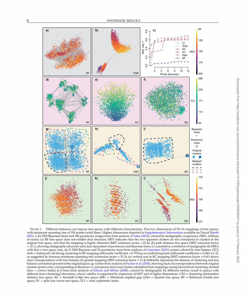
Because different metrics capture different aspects oftree similarity, the tree spaces they define can exhibitvery different properties. The strong connection betweentree shape and the KC distance means that differencesin the degree of tree balance are often the primaryfeature of KC tree spaces, but do not characterizespaces constructed using other metrics (e.g., Fig. 1d–f).Mappings of RF spaces often stand out as particularlydifferent to those of other spaces; in many cases, theunderlying RF space lacks structures, such as clustersand correlation with stratigraphic fit, which are presentin all other tree metric spaces (Fig. 1a–c, g–l; Smith 2021);though in other cases (e.g., Fig. 1d), RF mappings exhibitstructure that is not evident in other spaces.

ClustersIf a data set displays genuine clustering structure, then

it is desirable for clusters to be clearly distinguished. Treespaces constructed on the quartet, KC, and SV metricsexhibit the most prominent clusters, whereas clusteringis least defined in RF tree spaces (Fig. 2a). Better-definedclusters exhibit a higher silhouette coefficient, increasingthe number of cases in which “reasonable” clusteringstructure (silhouette coefficient > 0.5) can be identified(Fig. 2c). For tree spaces that exhibit “reasonable”clustering, the clustering solution identified is verysimilar (VI ≤ 0.01 bits) under all distance metrics except

TABLE 1. Performance of selected tree distance metrics against tests of tree distance behavior

Ranking Best 2 3 4 5 Worst

Length of move: mis-orderings (0–545) RF (0) CID (8) QD (94) Path (126) SV (188) KC (360)No. leaves moved: inconsistent cases (0–289) = CID (0) = Path (0) SV (2) KC (11) QD (17) RF (289)Saturation: 11-leaf trees with max score (1–100,000) = CID (1) = QD (1) = Path (1) = SV (1) KC (3) RF (86,336)Sensitivity: distinct values (100,000–1) CID (28,939) KC (581) SV (541) Path (302) QD (200) RF (6)Shape independence: r2 (0–1) QD (10−4) CID (0.0079) RF (0.024) SV (0.055) KC (0.35) Path (0.48)Balance independence: r2 (0–1) RF (0.0001) QD (0.0007) CID (0.0014) SV (0.004) Path (0.027) KC (0.375)Cluster recovery: mean rank (1–25) CID (7.2) QD (9.8) RF (10.9) KC (14.1) Path (16.3) SV (16.9)Bullseye subsampling successes (1000–0) CID (650) Path (633) QD (626) SV (588) KC (573) RF (410)Bullseye miscoding successes (1000–0) CID (941) QD (809) RF (781) SV (709) Path (704) KC (598)SPR rearrangement: Kendall’s � (1–0) CID (0.771) RF (0.744) QD (0.739) SV (0.608) Path (0.536) KC (0.482)Random distances interquartile range (% of median) QD (1.6) CID (1.6) SV (2.2) Path (18.8) KC (35.2) RF (n/a*)

Note: Parentheses denote range of possible scores for each measure (best to worst). Note that random tree pairs obtain the maximum possibleRF distance, resulting in a zero interquartile range (*). Full details and results in Smith (2020a) and Smith (2021).CID = clustering information distance; KC = Kendall–Colijn distance; QD = quartet distance; RF = Robinson–Foulds distance; SV = split sizevector distance.

Dow



https://academic.oup.com/sysbio/article-lookup/doi/10.1093/sysbio/syab100#supplementary-data

http://dx.doi.org/10.5061/dryad.kh1893240




a)

RF

b)

Path 2 4 6 8 10 12

0.0

0.2

0.4

0.6

0.8

PCoA dimension

MIG

, Adj

. r²

c)

CIQ'tetKCSVPathRF

MIG:

305

175

150

128

66

d)

RF

e)

KC

f)

QD

TCI:

56

114

171

228

286

g)

RF

h)

SSV

i)

QD

Bayesiantrees

Parsimonytrees

Originalclusters

Mappedclusters

j)

RF

k)

KC

l)

QD

MIG:

231

165

158

153

120

FIGURE 1. Different distances can impose tree spaces with different characteristics. First two dimensions of PCoA mappings of tree spaces,with minimum spanning tree of 350 points (solid lines). Higher dimensions depicted in Supplementary Information available on Dryad (Smith2021). a, b) 2500 Bayesian (dots) and 100 parsimony (rings) trees from analysis of Yates (2003), colored by stratigraphic congruence (MIG, millionsof years); (a) RF tree space does not exhibit clear structure; MST indicates that the two apparent clusters do not correspond to clusters in theoriginal tree space, and that the mapping is highly distorted (MST extension factor =22.4); (b) path distance tree space (MST extension factor=12.1), showing stratigraphic structure and clear separation of parsimony and Bayesian trees; (c) cumulative correlation of stratigraphic fit (MIG)with first n tree space axes; (d–f) 2500 Bayesian and 54 parsimony trees from analysis of Carpenter (2001); points colored by tree balance (TCI;dark = balanced): (d) strong clustering in RF mapping (silhouette coefficient =0.70) has no underlying basis (silhouette coefficient =0.040�0.2),as suggested by tortuous minimum spanning tree (extension factor =33.3); (e) vertical axis in KC mapping (MST extension factor =9.61) showsclear correspondence with tree balance; (f) quartet mapping (MST extension factor =13.4) faithfully represents the absence of clustering and treebalance correlation present in the original space; (g–i) trees from analysis of Fischer et al. (2016), showing (lack of) correspondence between originalclusters (point color, corresponding to Bayesian vs. parsimony trees) and clusters identified from mappings (using hierarchical clustering; dashedlines = convex hulls); (j–l) trees from analysis of Schoch and Milner (2008), colored by stratigraphic fit; different metrics result in spaces withdifferent (non-clustering) structures, whose validity is supported by inspection of MST and of higher dimensions. CID = clustering informationdistance tree space; KC = Kendall–Colijn tree space; MIG = Minimum implied gap; Q’tet = Quartet tree space; RF = Robinson–Foulds treespace; SV = split size vector tree space; TCI = total cophenetic index.

Dow







the quartet, KC, and SV metrics (VI with each othermetric ≥ 0.03, ≥ 0.02, and ≥ 0.01 bits, respectively)(Fig. 2e).

The highest silhouette coefficients are typicallyobtained with hierarchical clustering (Fig. 2g,h). Where“reasonable” structure is present, K-means and parti-tioning around medoids (PAM) tend to produce similarresults to each other (VI =0.0094 bits) and to hierarchicalclustering (VI =0.011 bits) (Fig. 2f). Spectral clusteringtends to resolve clusterings that are somewhat differentfrom those of other methods (VI ≥ 0.021 bits) (Fig. 2f),often with lower silhouette coefficients; these clustersoften fall below the threshold for “reasonable” structure,even in some instances where “strong” structure (silhou-ette coefficient > 0.7) is recovered by other methods.

Effects of MappingThe degree of clustering is often exaggerated in two-

dimensional mappings of tree space. Silhouette coeffi-cients on clusterings calculated from mapped distancesare typically higher by around 0.25 (Fig. 2a–d), withthe effect that “weak” structure in the original treespace often appears “reasonable” when mapped, and“reasonable” structure often appears “strong” (for anextreme example see Fig. 1d, noting how the MST hints ata discrepancy between mapped and original distances).This said, the existence of “reasonable” structure in theoriginal tree space does not guarantee that clusteringwill be evident in a two-dimensional mapping. Ofthe 116 tree spaces (11% of 128 data sets × eightdistance metrics) with at least “reasonable” clusteringstructure, 19 two-dimensional PCoA mappings and66 two-dimensional t-SNE mappings display no morethan “weak” structure, meaning that genuine clusterscannot be distinguished. Even where clustering structureexists in both the original tree space and its two-dimensional mapping (97 PCoA mappings; 50 t-SNEmappings), dimensionality reduction often changes thecomposition of clusters markedly (VI > 0.25 bits in 39%of PCoA and 94% of t-SNE mappings) (Fig. 1g–i).Clusterings are identical in only 53% of PCoA and6% of t-SNE mappings (Fig. 3a,b). Changes in clustercomposition are particularly pronounced in mappingsof the Euclidian vector-based and quartet distances, andin PCoA mappings of RF distances (Fig. 3a,b).

More broadly, tree spaces defined by different metricshave different propensities for mapping. Mappings of RFtree spaces exhibit greater distortion than mappings ofother spaces, reflected by lower trustworthiness and con-tinuity metrics, higher stress, more extended MSTs, andless correlation with original distances (Fig. 3c–e).To obtain a trustworthy and continuous mapping ofRF distances, it is often necessary to plot at leastone dimension more than with other distance metrics(Fig. 3c). Conversely, KC tree space, and to a lesserextent the quartet, path, and SV spaces, can be mappedin a more trustworthy and continuous fashion thaninformation-theoretic tree spaces, often attaining the

same degree of distortion with one or even two fewerdimensions (Fig. 3c)—reflected by lower stress, lessextension of the MST, and a higher correlation betweenoriginal and mapped distances (Fig. 3c–e). Thoughmappings of KC, SV, and quartet tree spaces are the mostfaithful to the original distances, these mappings tendto exhibit a lower intrinsic dimensionality (Fig. 3g) and,for the SV and quartet spaces, a correspondingly weakercorrelation with stratigraphic congruence (Fig. 3f)—suggesting that the improved mapping may reflect asimpler original tree space that fails to represent certainaspects of tree similarity.

Mapping MethodIn most cases, PCoA, Kruskal-1, and Sammon map-

pings of tree space differ only in small details, a recurrenttheme being that Sammon maps often contain outliersplotted far from the majority of trees (Smith 2021). Thesemethods consistently attain the highest correlation withthe original distances and stratigraphic congruence, andhigh levels of trustworthiness and continuity (Fig. 4),indicating that these methods map the original tree spacewith the least distortion.

The lower correlation between other methods andoriginal distances reflects their different motivations—for example, contraction of large distances may be seenas justified if it allows a clearer mapping of spatialrelationships on a more local scale. In the case of t-SNE, this trade-off results in mappings with highertrustworthiness and continuity and with less-extendedMSTs. The opposite is true for Laplacian eigenmapping,diffusion mapping, or CCA. t-SNE, Laplacian eigenmap-ping, and diffusion mapping each exhibit prominentand idiosyncratic structure (which may or may notcorrespond to structure in the original tree space),whereas a typical CCA map simply depicts a separate,approximately hyperspherical cloud corresponding toeach “reasonable” cluster, with no clear evidence of anyfurther structure (Smith 2021).

Number of DimensionsRF, path, and information-theoretic tree spaces have

particularly high intrinsic dimensionalities (median ≈5; Fig. 3g). Correspondingly, in the great majority ofdata sets considered herein, two-dimensional mappingsexhibit low (�0.95) trustworthiness and continuityvalues. Mapping additional dimensions depict distancesmore accurately and often reveals additional structure(Figs 4 and 5): it is not uncommon for a single highdimension of tree space to account for 50% of thevariance in stratigraphic fit (Fig. 5). In contrast, the lowerdimensionalities of quartet (3.8), KC (2.7), and SV (2.5)tree spaces indicate that these spaces might often bemapped to three or even two dimensions with littledistortion. But even with these metrics, two dimensionsare enough to produce mappings with high values(>0.95) of trustworthiness and continuity only wherethe number of distinct tree topologies within the tree

Dow






Cluster definition

Best

silh

ouet

te c

oeffi

cien

t0.

00.

20.

40.

60.

8 2D PCoA cluster defn.

Best

silh

ouet

te c

oeffi

cien

t0.

00.

20.

40.

60.

8

RF MS PI CI Pt KC SV Q

Number of clusters

Tree distance metric

Num

ber o

f stu

dies

040

8012

0

1 1 1 1 1 1 1 1

2 2 2 2 2 2 2


2D PCoA clusters

Tree distance metricN

umbe

r of s

tudi

es0

4080

120

11 1 1 1

1

11

2

2 2 2 22

2

2

3 3

3

34 4

Diff by tree distance

Variation of information / mbits

6

6

8

8

2

2

8

8

2

2

0

0

11

11

6

6

3

3

3

3

16

16

19

19

21

21

21

21

18

18

21

21

15

15

13

13

13

13

10

10

26

26

36

36

30

30

28

28

28

28

32

32

49

49

28

28

RF

MS

PI

CI

Pt

KC

SV

Q

Diff by cluster method

Variation of information / mbits

9.38

9.38

11.8

11.8

11.4

11.4

26.8

26.8

20.9

20.9

28.5

28.5

K−mns

PAM

Hier.

Spec.

Cluster definition

Clustering method

Silh

ouet

te c

oeffc

ient

K−mns PAM Hier. Spec.

−0.2

0.2

0.6

K−mns PAM Hier. Spec.

Best clustering method

Clustering method

Num

ber o

f tre

e sp

aces

020

6010

0

a) b)

c) d)

e) f)

g) h)

FIGURE 2. Methods for optimal clusterings. a, b) Strength of clustering (silhouette coefficient) across all 128 tree sets under each tree distancemetric in (a) original tree space; (b) 2D PCoA mapping. Box plots denote median and interquartile range; strong evidence that medians differexists where notches do not overlap. c, d) Number of clusters in optimal clustering under each tree distance method, calculated from (c) originaldistances; (d) 2D PCoA mapping. Tree sets lacking “reasonable” structure (i.e., silhouette coefficients < 0.5) are taken to exhibit a single cluster.e, f) Mean difference (variation of information) between optimal clusterings obtained under (e), each tree distance metric (f), each clusteringmethod, from data sets exhibiting at least “reasonable” clustering structure. Brighter colors represent greater differences. g) Definition (silhouettecoefficient) of optimal clustering obtained under each clustering method, summarized for all distances and tree sets. Bars denote medians andinterquartile ranges. h) Method obtaining clustering with highest silhouette coefficient, across all tree spaces with at least “reasonable” clusteringstructure (silhouette coefficient > 0.5).

Dow






Varia

tion

of in

form

atio

n / b

its


01

23

42D PCoA

Varia

tion

of in

form

atio

n / b

itsRF MS PI CI Pt KC SV Q

01

23

4

2D t−SNE Dim

. whe

re tr

ust.

& co

nt. >

0.9

5


24

68

1012

MST

ext

ensi

on fa

ctor


12

510

3D PCoA

2 4 6 8 10 12

0.0

0.2

0.4

0.6

0.8

1.0

Dimension

True

dis

tanc

e, A

djus

ted

r²

Mean1 Std. Dev.

Dimension

MIG

, Adj

uste

d r²

0.0

0.2

0.4

0.6

0.8

1.0

1 3 5 7 9 11

RFMSIPI

CIPathKC

SVQ'tet

Tree distance metric

Intri

nsic

dim

ensi

onal

ity


05

1015

a) b) c) d)

e) f) g)

FIGURE 3. Quality of tree space mappings based on underlying tree distance method. a, b) Difference between original and mappedclusterings, in tree spaces that contain at least “reasonable” clustering structure (silhouette coefficient > 0.5); (c) number of dimensions wheretrustworthiness and continuity are each > 0.95; (d) length of minimum spanning tree relative to shortest possible in 3D PCoA mappings;increasing values indicate more distorted mappings; (e, f) cumulative correlation coefficient (r2) between Sammon mapping axes and (e) originaltree distance; (f) stratigraphic congruence (MIG); (g) correlation dimension of tree spaces. Box and whisker plots depict medians and interquartileranges; where notches do not overlap, strong evidence exists that medians differ.

2 4 6 8 10 12

0.5

0.6

0.7

0.8

0.9

1.0

Dimension

Trus

tw. ×

con

tinui

ty

2 4 6 8 10 12

105

21

Dimension

MST

ext

ensi

on fa

ctor

2 4 6 8 10 12

0.0

0.2

0.4

0.6

0.8

1.0

Dimension

Cor

r. w

/ tru

e di

stan

ce

2 4 6 8 10 12

0.0

0.2

0.4

0.6

0.8

1.0

Dimension

Cor

rela

tion

with

MIG

t−SNE PCoA Sammon CCA Dif. map Lap. Eig.

a) b) c) d)

FIGURE 4. Effectiveness of mapping methods. a) Trustworthiness × continuity; (b) minimum spanning tree extension factor; (c) correlationwith original distances (adjusted r2); and (d) correlation with stratigraphic congruence (MIG, adjusted r2). Lines depict median and interquartilerange. Kruskal-1 mappings (omitted for clarity) behave equivalently to PCoA. t-SNE mapping results only available for first three dimensions.

space is minimal (<30). A third dimension is enoughto attain these values only in a minority of cases, andnever in data sets containing trees with twenty or moreleaves; the majority of analyses require at least fourto five dimensions for a trustworthy and continuousrepresentation (Figs 3c and 4a).

The intrinsic dimensionality of a space also reflectsproperties of the data sets under examination. Underall distance metrics, it is negatively correlated with thelog ratio of the number of characters to the number of

taxa (r2 =0.1−0.24,P<10−3; Supplementary Fig. S1).Dimensionality correlates positively with the totalnumber of taxa in RF space (r2 ≈0.1,P<10−3), andnegatively in quartet space (r2 ≈0.1,P<10−3), butdisplays no significant correlation in other metricspaces. Tree space dimensionality is positivelycorrelated with the number of unique trees underthe RF (r2 =0.24,P<10−3) and information-theoretic(r2 =0.11−0.14,P<10−3) distances, and (more weakly)

Dow








831

652

584

574

528R

&D M

IG

Xu et al. MIG

530

382

320

292

200

Russell & Dong 1993Xu

et a

l. 20

18

Dimension 1

Dimension 2

Dimension 4

Dimension 5

Xu et al.Russell & Dong

Dimension

Adj.

r²

1 2 3 4 5 6

0.0

0.3

0.7

1.0

FIGURE 5. Structure “hidden” in higher dimensions. First six dimensions of phylogenetic information distance PCoA tree space, showing 2500Bayesian trees (dots) and single most parsimonious tree (circles). Results from: bottom left, Russell and Dong (1993); top right, Xu et al. (2018).Structural features evident in higher dimensions are not apparent within the first two dimensions (top left corner), particularly with regard tostratigraphic congruence, which is strongly correlated with higher dimensions of tree space (bottom right).

the path and KC distances (r2 <0.03,P=0.03−0.04);but no such correlation exists under the SV and quartetdistances.

DISCUSSION

When analyzing the distribution of phylogenetic trees,three decisions prove highly consequential: the distance

metric used to construct a tree space; how clusters areidentified; and how tree space is visualized.

Distance MetricTree spaces are defined with reference to an under-

pinning distance metric. Fundamentally, a distancemetric should afford smaller distances to trees thatare more similar with respect to the properties under

Dow






consideration—different metrics can impose profoundlydifferent tree spaces (Fig. 1), so a tree space will onlybe illuminating if its underlying metric is relevant to itsapplication.

Robinson–Foulds spaces.—The properties of the RF dis-tance that produce poor performance in a range ofpractical settings [Table 1; Steel and Penny (1993); Smith(2020a)] are particularly relevant to the constructionof tree spaces: its low resolution imposes an over-quantized and thus “gappy” space; its ready saturationmeans that even quite similar trees can be assigned themaximum distance; and its sensitivity to the relocation ofa single group or leaf means that a subset of otherwisesimilar trees will be allocated unrepresentatively largedistances. In part, the high intrinsic dimensionality ofRF tree spaces (Fig. 3g) reflects the distortions necessaryto accommodate these phenomena. Correspondingly,the RF mappings analyzed in this study often containartifacts, fail to depict structures that are apparent underother metrics, recover weaker clustering structure, andare highly distorted (Figs 1–3). As such, it is difficultto be confident that interpretations of RF tree spacesaccurately represent any meaningful aspect of treesimilarity.

Euclidian vector-based spaces.—At first blush, tree spacesdefined on Euclidian vector-based metrics look likepromising alternatives—particularly with regard to thehigh fidelity of their low-dimensional mappings (Figs 1–3). The particularly low intrinsic dimensionalities of theKC and SV metrics (Fig. 3g) allow the majority of theirtree space structure to be represented in three or eventwo dimensions (Fig. 3c, e). These two metrics also standout for the clear definition of their clustering structure(Fig. 2a–d), even if this maps less faithfully into fewdimensions (Fig. 3a, b).

However, such clustering structure often fails tocorrespond to artificial structure known to character-ize the true distribution of trees (Table 1, “clusterrecovery”). Lower intrinsic dimensionalities seem to beaccomplished by downplaying phylogenetic differencesbetween trees, resulting in simplistic spaces whosestructures emphasize the contribution of tree shape. Asubstantial proportion of the variance in KC distancesreflects the degree of tree balance (Table 1), meaningthat KC tree spaces are often dominated by a singledimension that discriminates balanced from unbalancedtrees (as in Fig. 1e), independently from how leaveshappen to be labeled. The contribution of tree shape tothe path and SV metrics, though more nuanced, results incomparable behavior. Because the relative contributionsof phylogenetic and shape-based factors are not explicitin the definition of these vector-based metrics, it isdifficult to disentangle their contribution to the structureof tree space. Consequently, Euclidian vector-based treedistances, and the KC metric in particular, are poorlysuited to questions of evolutionary relationships.

Quartet and information-theoretic metrics.—Thougheach have subtly different emphases, quartet andinformation-theoretic distances increase monotonicallyas tree topologies undergo increasing amounts ofdeformation (Table 1), making them inherently relevantto questions concerning the similarity of evolutionaryrelationships between cladograms (Smith 2020a). TheMS, PI, and CI distances produce broadly similartree spaces with similar clustering, dimensionality,and mapping characteristics (Figs. 1–3), so are treatedtogether here. Quartet tree spaces exhibit a morepronounced clustering structure (Fig. 2a–d) and a lowerintrinsic dimensionality (Fig. 3g) than information-theoretic tree spaces, meaning that they can producemore information-rich maps using fewer dimensions(Fig. 3).

In many cases, being able to obtain a tree spacethat discriminates clusters more readily and whichrequires one fewer dimension to obtain a given levelof trustworthiness and continuity will more than offsetthe slightly poorer performance of the quartet metricagainst the benchmarks of Smith (2020a) and Table 1,and justify its significantly greater running time—measured in hours rather than minutes for many of thedata sets examined here. On the other hand, clustersobtained using information-theoretic distances are typ-ically rendered more faithfully in mappings. Confidencethat interpreted structure genuinely characterizes theunderlying trees will be greatest if its presence can bedemonstrated in both quartet and information-theoretictree spaces, which offer complementary views on thephylogenetic similarity of trees.

ClustersOne motivation for tree space analysis is the identifica-

tion of subsets of trees that are more similar with respectto the evolutionary histories they imply. This objectiveis most readily met when the distance from whichclusters are calculated measures that property directly.Clusters identified through the visual inspection oftwo-dimensional tree space mappings will group treesaccording to mapped distances, which are an opaquefunction of original tree-to-tree distances, distorted ina manner that is particular to each mapping techniqueand influenced by all other tree-to-tree distances underconsideration. Such clusters thus have no straight-forward interpretation in their own right, except asapproximations to the clustering structure imposed bythe original, undistorted distances.

My results show that clusters derived from mappeddistances are poor approximations to clusters based onmeasured distances. In the majority of RF, SV, and quar-tet tree spaces in which “reasonable” or better structureis present in both original and mapped spaces, clustersderived from original versus mapped distances differsubstantially in their constitution (median VI > 0.2 bits;Fig. 3a). Mapping a tree space into two dimensions usingPCoA consistently exaggerates clustering structure,

Dow






causing a mean increase in silhouette coefficient of 0.3(Fig. 2a,b)—enough that maps may depict “reasonable”or even “strong” structure where original, undistorteddistances exhibit only “weak” structure that “may notbe genuine.” Correspondingly, many mappings depictmultiple clusters that lack “reasonable” support inthe underlying tree space (Fig. 2c,d). It is thereforeinadvisable to assume that clusters interpreted fromtwo-dimensional mappings represent genuine structure.Even if such clusters sometimes happen to group treeswith certain characteristics in common, it is difficult tosee how they would be preferable to a clustering derivedfrom a direct and explicit measure of those specificcharacteristics.

Where a tree space does exhibit clustering structure,a secondary objective is to assign trees to clustersin a fashion that minimizes overlap between clusters,thus maximizing the silhouette coefficient. Hierarch-ical clustering usually performs best against this cri-terion (Fig. 2h), though partitioning around medoidsand K-means clustering occasionally produce the best-defined clustering. Differences between the clusteringsrecovered by different methods tend to be relativelysmall (Fig. 2f), and which method is most appropriatewill depend on the specific structure within a givendata set and the emphases of the particular clusteringmethods: for example, K-means and PAM are veryeffective when clusters are consistent shapes or sizes, butcan produce unexpected results when this assumptionis violated (MacKay 2003; Hastie et al. 2009). Suchfactors may contribute to the poor performance ofspectral clustering in these data sets (Fig. 2f–h), despiteits accurate recovery of pre-defined clusters of treesin other settings (Gori et al. 2016): the geometry ofthese artificial tree spaces may align better with thestrengths of spectral clustering. Though the use of asingle clustering method is unlikely to mislead, theapplication of multiple methods provides additionalopportunities to maximize the silhouette coefficient, andthus to better appreciate the clustering structure of a treeset.

Visualizing Tree SpacesDifferent mapping techniques have different motiv-

ations, and thus differ markedly in the structure theydepict. Mapping has an order of magnitude more impacton the clustering structures perceived—the easiestaspect of structure to quantify—than the measurementof tree distance or the method of cluster detection(Figs 2e–f and 3a,b).

PCoA, Sammon, and Kruskal-1 mappings have asimilar philosophy: they seek to minimize the stressinduced by a mapping by minimizing a measure ofdistortion that penalizes mismatches between originaland mapped distances. Interpretation of such mappingsis straightforward: mapped distances are approximatelyproportional to the true distances between trees. (Thisdoes not mean that mapped areas are proportional to

original hypervolumes—see Mammola (2019).) In linewith this common principle, and despite the poten-tial shortcomings of PCoA (Lee and Verleysen 2007),these methods often result in very similar mappings—consistent with some other results from simulated andreal data sets (van der Maaten et al. 2009; Ekman andBlaalid 2011). As PCoA is significantly faster to calculate,its status as the most widely used mapping methodseems justified.

CCA mapping likewise seeks to minimize stress—butthe cost function employed aims not to faithfully reflectoriginal distances, but rather to produce a “revealing rep-resentation” of the data, with an emphasis on facilitatingthe visual recognition of clustering (Demartines andHerault 1997). The clear depiction of clustering structureseems here to be obtained by largely discarding otheraspects of tree space structure. In contrast to the resultsof Wilgenbusch et al. (2017), CCA-mapped distancesexhibited lower correlation with original distances, andCCA mappings exhibited lower trustworthiness andcontinuity than PCoA, Sammon, and Kruskal-1 map-pings (Fig. 4). This difference may reflect idiosyncrasiesof the tree sets being examined: for example, theWilgenbusch et al. (2017) tree sets cluster according to thegene from which trees had been inferred, so emphasizingthe distinction between clusters captures relatively moreof the variation in tree-to-tree distances than in data setswith weak clustering structure.

Diffusion mappings and Laplacian eigenmappingsattempt to identify a lower-dimensional manifold thatunderlies the high-dimensional space; the poor perform-ance of explicitly manifold-learning methods relative toother mapping techniques (Fig. 4) suggests that the setsof optimal trees examined herein are not associated withany manifold, or sample the manifold at too low a densityfor its inferred structure to improve mapping (Vennaet al. 2010).

Finally, t-SNE obtains very high levels of trustworthi-ness and continuity, at the expense of a weak correlationbetween mapped and original distances (Fig. 4). As such,the interpretation of t-SNE mappings is not intuitive:distances between clusters, and the sizes of clusters,may not be representative; and t-SNE mappings candisplay apparent structure in data sets known to behomogeneous (Wattenberg et al. 2016). These proper-ties characterize many of the t-SNE maps generatedherein (see for example studies 20, 36, 89 in Smith2021), meaning that the capacity of t-SNE mapping torepresent local structure must be weighed against thedanger of misinterpretation. This risk can be reducedby exploring different values of the “perplexity” and“epsilon” parameters that govern the structure of t-SNEmappings, and comparing results to a PCoA mapping.

Dimensionality.— Tree spaces inherently exist in manydimensions. More trees tend to produce more com-plicated structure with more intrinsic dimensions, aspreviously noted by Wilgenbusch et al. (2017), andobserved here under the RF and information-theoreticdistances. Tree sets derived from data sets with a

Dow






low character:taxon ratio also tend to exhibit higherdimensionalities, perhaps because matrices containingfewer characters constrain relationships less decisively:a broader posterior distribution of tree topologies willencompass a larger region of tree space and thusencounter more distortion when mapped (just as a mapof the globe is more distorted than a cartographic mapof a smaller region).

The dimensionality of tree space is also influencedby the choice of distance metric (Fig. 3). Whereas treespaces with more intrinsic dimensions have the capacityto contain more sophisticated and instructive structure,they are harder to faithfully depict in few dimensions.This trade-off does not have a natural optimum, as theutility of a tree space is not a simple function of itsdimensionality. KC and SV tree spaces obtain a lowdimensionality by downplaying phylogenetic aspectsof tree similarity. Although mappings produced afterdiscarding relevant features of tree space may be lessdistorted, this is unlikely to compensate for the concom-itant loss of information: at the extreme, a dimensionalityof zero can be obtained by a metric that assigns all pairsof trees a distance of zero. On the other hand, the merefact that more dimensions are present need not makea tree space more instructive: a metric that assigns allpairs of trees a unit distance can produce a meaninglesstree space with many dimensions. Analogously, thelow sensitivity and rapid saturation of the RF distance(Table 1) mean that it allocates many tree pairs identicalscores, potentially increasing the number of dimensionsnecessary to map RF spaces without distortion (Fig. 3c–e) without a corresponding gain in utility. In contrast, thelower dimensionality of quartet tree space relative to treespaces defined by information-theoretic distances seemsnot to reflect a substantial difference in how well the met-rics measure the phylogenetic similarity of cladograms(Table 1). Consequently, the lower amount of distortionintroduced when quartet spaces are mapped (Fig. 3c–f) is a reason to prefer this distance for visualization,so long as examination of higher dimensions of bothquartet and information-theoretic spaces confirms thata low-dimensional mapping adequately summarizesstructure.

Even under the quartet distance, however, the majorityof data sets require more than 3 (median: 5) dimensionsto attain levels of trustworthiness and continuity greaterthan 0.95 (Fig. 3c). Humans are less able to perceivemetric distances in three-dimensional visualizationsthan in two dimensions (Kjellin et al. 2010), and three-dimensional displays are ineffective for estimating relat-ive positions (Tory et al. 2006). Mappings that requiremultiple dimensions may thus fail in their objectiveof making distances easier to visualize. Wilgenbuschet al. (2017) take the more optimistic position thattwo-dimensional mappings capture the most importantaspects of tree space structure, including clustering. Inpractice, I suspect that individual data sets each occupytheir own position between these extremes. Althoughtwo-dimensional maps tend to exaggerate the degree ofclustering—leading to the misidentification of clusters

(Figs 1d, 2a–d, and 3a,b), and in some cases, the failure todepict aspects of tree space structure that are relevant tointerpretation (Fig. 5)—whatever structure is portrayedby a two-dimensional plot can at least by decipheredat a glance, in contrast to more cognitively taxingportrayals of higher-dimensional space, which must stillultimately be perceived through the two dimensions ofthe retina. The potential for misinterpretation can bereduced by plotting the MST (e.g., Fig. 1d), by markingclusters that are statistically supported by the originaldistances, by evaluating how well a low-dimensionalmapping conveys tree-to-tree distances, and by carefullyexamining higher dimensions for evidence of additionalstructure.

RecommendationsIn summary, commonly used practices are generally

inadequate for the interpretation of the phylogenetictree spaces explored herein. The KC and RF metrics donot directly measure trees’ phylogenetic similarity; theirassociated tree spaces are poorly suited to phylogeneticquestions. Clusters identified by visual inspection ofmappings are likely to misrepresent the true structureof a tree set. Two dimensions are seldom sufficientto convey the full structure of tree space, and two-dimensional mappings should be viewed with suspicionunless shown to exhibit high values of continuity andtrustworthiness; a low correlation between original andmapped distances indicates that the interpretation of amapping may require additional care.

The 128 tree sets studied herein include multipleexamples where standard practice would lead to invalidconclusions. For instance, Wright and Lloyd (2020)correctly interpret the RF space of trees from Yates (2003)(Fig. 1a; cf. fig. 1C in Wright and Lloyd (2020)) as exhib-iting no relationship with stratigraphic congruence—yet a strong relationship is present in all other metricspaces (see Fig. 1b and Smith (2021)). Similarity, two-dimensional mappings of Russell and Dong (1993) orXu et al. (2018) tree spaces (Fig. 5) contain no hint ofthe significant correlation with stratigraphic congruencethat exists in higher dimensions. Strong clustering inthe mapped RF space of trees from Fischer et al. (2016)is entirely an artifact of mapping: no correspondingstructure exists in the original distance matrix. Theseare not isolated instances, but examples that illustraterecurrent patterns evident across all examined studies;and there is no obvious reason that the tree setsanalyzed here should be particularly intractable to treespace analysis. With the caveat that “landscapes” oftrees selected using different optimality criteria or fromdifferent sources of data may exhibit different properties,these results raise serious concerns over the validity ofprevious presentations of tree spaces.

To minimize artifacts when analyzing the distributionof cladograms, I recommend that tree space analysisemploys the CI or quartet distances—ideally, both. Thesedistances are sensitive to differences in the evolution-ary relationships implied by cladograms, but not to

Dow






factors such as tree shape that are irrelevant to mostphylogenetic questions. Information-theoretic distances(particularly the CI distance) measure the similaritybetween cladograms more effectively than the quartetdistance and have a higher intrinsic dimensionality.Insofar as this higher dimensionality denotes a moreinformation-rich tree space, the CI distance is well suitedto the identification of clusters of trees; moreover, theseclusters tend to retain their identity when mapped. Onthe other hand, the lower dimensionality of quartet treespace means that it suffers less distortion when mapped.Structure evident in both metric spaces might warrantadditional confidence.

Except where clustering is conducted for a separatepurpose (Gori et al. 2016)—for instance, when usingclusterings to generate summary trees (Stockham et al.2002)—clusters should be identified objectively fromoriginal tree distances. The clustering with the highestsilhouette coefficient can be considered the best repres-entation of the underlying structure, provided that thiscoefficient is high enough to indicate that the structureis meaningful (>0.5). Hierarchical clustering often findsthe best clustering, but as the optimal method dependson the nature of clustering structure, I encourage theuse of multiple clustering methods. Depicting the bestclustering on mappings (as in Fig. 1g–i) reduces thepotential for misinterpretation where mappings do notreflect the structure of the original tree space.

The optimal mapping method will depend on thepurpose of the visualization. PCoA maps—which tendto closely resemble Sammon and Kruskal mappings, butare much faster to compute—tend to reproduce originaltree-to-tree distances most faithfully, making them easyto interpret, while also depicting structure consist-ently (high trustworthiness and continuity); as such,they are an obvious choice for instructive mappings.Alternatively, t-SNE maps emphasize local structuralrelationships, though their interpretation can be counter-intuitive; whereas CCA maps depict cluster membershipwhile downplaying other structural features.

Whichever mapping method is employed, it is import-ant to evaluate the quality of the mapping: high (>0.95)values of the trustworthiness and continuity measuresare desirable, as is a good correlation with originaldistance metrics. Even if MSTs can help to visually assessthe degree of distortion, it is not possible to be confidentthat any apparent structure is genuine unless the qualityof a mapping is explicitly documented. Of course, thesemetrics will be invalid, and distances misrepresented,unless plotting software is configured to plot x and yaxes to the same scale.

These recommendations are drawn from a limitedsample of morphological data sets; it is likely that treesets obtained from different data sets using differentmethods will occupy tree spaces with different prop-erties. Nevertheless, the degree to which methodolo-gical decisions can influence the interpretation of treespace represents a strong argument for conducting anddocumenting basic checks to establish that presented

results truly represent the underlying structure of thehigh-dimensional tree space.

To facilitate best practice in the construction,evaluation, and interpretation of tree space, I haveproduced a “point-and-click” graphical interfacewithin R—installed using install.packages(’TreeDist’) and launched by executing thecommand TreeDist::MapTrees(). This softwareallows users to upload trees, select tree distance,mapping and clustering methods, and generate high-dimensional mappings, with real-time evaluationsof mapping and clustering quality to ensure thatinterpretations truly reflect the underlying distributionof phylogenetic trees.

SUPPLEMENTARY MATERIAL

Data available from the Dryad Digital Repository:http://dx.doi.org/10.5061/dryad.kh1893240.

ACKNOWLEDGMENTS

Reviews from Michelle Kendall and four anonymousreferees, comments from editor Sebastian Höhna, anddiscussions with Andrew Millard, Matthias Sinnesael,and April Wright, stimulated the research and improvedthe manuscript. Nura Kawa provided scripts for spectralclustering.

CONFLICT OF INTEREST

I disclose no conflicts of interest.

REFERENCES

Amenta N., Klingner J. 2002. Case study: visualizing sets of evolution-ary trees. In: Wong P.C., and Andrews K., editors. IEEE symposiumon information visualization, 2002. Los Alamitos (CA): INFOVIS2002. p. 71–74.

Anderson A.J.B. 1971. Ordination methods in ecology. J. Ecol. 59:713–726.

Bastert O., Rockmore D., Stadler P.F., Tinhofer G. 2002. Landscapes onspaces of trees. Appl. Math. Comput. 131:439–459.

Belkin M., Niyogi P. 2003. Laplacian eigenmaps for dimensionalityreduction and data representation. Neural Comput. 15:1373–1396.

Bien J., Tibshirani R. 2011. Hierarchical clustering with prototypes viaminimax linkage. J. Am. Stat. Assoc. 106:1075–1084.

Billera L.J., Holmes S.P., Vogtmann K. 2001. Geometry of the space ofphylogenetic trees. Adv. Appl. Math. 27:733–767.

Cailliez F. 1983. The analytical solution of the additive constantproblem. Psychometrika. 48:305–308.

Camastra F., Vinciarelli A. 2002. Estimating the intrinsic dimension ofdata with a fractal-based method. IEEE Trans. Pattern Anal. Mach.Intell. 24:1404–1407.

Carpenter K. 2001. Phylogenetic analysis of the Ankylosauria. TheArmored Dinosaurs. Bloomington: Indiana University Press. p.455–483.

Chakerian J., Holmes S. 2012. Computational tools for evaluatingphylogenetic and hierarchical clustering trees. J. Comput. Graph.Stat. 21:581–599.

Coifman R.R., Lafon S. 2006. Diffusion maps. Appl. Comput. HarmonicAnal. 21:5–30.

Dow



http://dx.doi.org/10.5061/dryad.kh1893240




Colijn C., Plazzotta G. 2018. A metric on phylogenetic tree shapes. Syst.Biol. 67:14.

Demartines P., Herault J. 1997. Curvilinear component analysis: a self-organizing neural network for nonlinear mapping of data sets. IEEETrans. Neural Netw. 8:148–154.

Ekman S., Blaalid R. 2011. The devil in the details: interactions betweenthe branch-length prior and likelihood model affect node supportand branch lengths in the phylogeny of the Psoraceae. Syst. Biol.60:541–561.

Estabrook G.F., McMorris F.R., Meacham C.A. 1985. Comparison ofundirected phylogenetic trees based on subtrees of four evolution-ary units. Syst. Zool. 34:193–200.

Fischer V., Bardet N., Benson R.B.J., Arkhangelsky M.S., FriedmanM. 2016. Extinction of fish-shaped marine reptiles associated withreduced evolutionary rates and global environmental volatility. Nat.Commun. 7:10825.

Garba M.K., Nye T.M.W., Boys R.J. 2018. Probabilistic distances betweentrees. Syst. Biol. 67:320–327.

Garba M.K., Nye T.M.W., Lueg J., Huckemann S.F. 2021. Informationgeometry for phylogenetic trees. J. Math. Biol. 82:19.

Goloboff P.A., Catalano S.A. 2016. TNT version 1.5, including a fullimplementation of phylogenetic morphometrics. Cladistics. 32:221–238.

Gori K., Suchan T., Alvarez N., Goldman N., Dessimoz C. 2016.Clustering genes of common evolutionary history. Mol. Biol. Evol.33:1590–1605.

Gower J.C. 1966. Some distance properties of latent root andvector methods used in multivariate analysis. Biometrika.53:325–338.

Gower J.C., Ross G.J.S. 1969. Minimum spanning trees and singlelinkage cluster analysis. J. R. Stat. Soc. Ser. C Appl. Stat.18:54–64.

Hartigan J.A., Wong M.A. 1979. Algorithm AS 136: a K-meansclustering algorithm. J. R. Stat. Soc. Ser. C Appl. Stat. 28:100–108.

Hastie T., Tibshirani R., Friedman J. 2009. The elements of statisticallearning: data mining, inference, and prediction. 2nd ed. New York:Springer-Verlag.

Hillis D.M., Heath T.A., St. John K. 2005. Analysis and visualization oftree space. Syst. Biol. 54:471–482.

Holmes S. 2006. Visualising data. Statistical problems in particlephysics, astrophysics and cosmology. In: Lyons L., Karagöz ÜnelM., editors. Proceedings of PHYSTAT05. London: Imperial CollegePress. p. 197–208.

Höhna S., Landis M.J., Heath T.A., Boussau B., Lartillot N., MooreB.R., Huelsenbeck J.P., Ronquist F. 2016. RevBayes: Bayesianphylogenetic inference using graphical models and an interactivemodel-specification language. Syst. Biol. 65:726–736.

Huang H., Li Y. 2013. MASTtreedist: Visualization of tree space basedon maximum agreement subtree. J. Comput. Biol. 20:42–49.

Jolliffe I.T. 2002. Principal component analysis. New York: Springer-Verlag.

Jombart T., Kendall M., Almagro-Garcia J., Colijn C. 2017. Treespace:statistical exploration of landscapes of phylogenetic trees. Mol. Ecol.Resour. 17:1385–1392.

Kaski S., Nikkilä J., Oja M., Venna J., Törönen P., Castrén E. 2003.Trustworthiness and metrics in visualizing similarity of geneexpression. BMC Bioinformatics. 4:48.

Kaufman L., Rousseeuw P.J. 1990. Partitioning around medoids(Program PAM). Finding groups in data: an introduction to clusteranalysis. Hoboken (NJ): John Wiley & Sons, Ltd. p. 68–125.

Kendall M., Colijn C. 2016. Mapping phylogenetic trees to revealdistinct patterns of evolution. Mol. Biol. Evol. 33:2735–2743.

Kjellin A., Pettersson L.W., Seipel S., Lind M. 2010. Evaluating 2D and3D visualizations of spatiotemporal information. ACM Trans. Appl.Percept. 7:1–23.

Kraemer G., Reichstein M., Mahecha M.D. 2018. dimRed andcoRanking—unifying dimensionality reduction in R. R J. 10:342–358.

Krijthe J.H. 2015. Rtsne: t-distributed stochastic neighbor embeddingusing a Barnes–Hut implementation. Comprehensive R ArchiveNetwork. Available from: https://github.com/jkrijthe/Rtsne.Accessed January 10, 2022.

Kruskal J.B. 1964. Multidimensional scaling by optimizing goodnessof fit to a nonmetric hypothesis. Psychometrika. 29:1–27.

Lee J.A., Verleysen M. 2007. Nonlinear dimensionality reduction. NewYork (NY): Springer Science & Business Media.

Leigh J.W., Schliep K., Lopez P., Bapteste E. 2011. Let them fall wherethey may: congruence analysis in massive phylogenetically messydata sets. Mol. Biol. Evol. 28:2773–2785.

Lewis P.O. 2001. A likelihood approach to estimating phylo-geny from discrete morphological character data. Syst. Biol.50:913–925.

Lloyd G.T., Wright A.M. 2020. Data from: Bayesian analyses inphylogenetic palaeontology: interpreting the posterior sample.Dryad, Dataset, doi:10.5061/dryad.zs7h44j4w.

MacKay D.J.C. 2003. Information theory, inference, and learningalgorithms. Cambridge: Cambridge University Press.

Maddison D.R. 1991. The discovery and importance of multiple islandsof most-parsimonious trees. Syst. Biol. 40:315–328.

Maechler M., Rousseeuw P., Struyf A., Hubert M., Hornik K.2019. Cluster: cluster analysis basics and extensions. Compre-hensive R Archive Network. Available from: https://CRAN.R-project.org/package=cluster.

Mammola S. 2019. Assessing similarity of n-dimensional hyper-volumes: which metric to use? J. Biogeogr. 46:2012–2023.

Meila M. 2007. Comparing clusterings—an information based distance.J. Multivar. Anal. 98:873–895.

Mir A., Rosselló F., Rotger L.A. 2013. A new balance index forphylogenetic trees. Math. Biosci. 241:125–136.

Monod A., Lin B., Yoshida R., Kang Q. 2018. Tropical geometry ofphylogenetic tree space: a statistical perspective. arXiv.:1805.12400.

Murtagh F. 1983. A survey of recent advances in hierarchical clusteringalgorithms. Comput. J. 26:354–359.

Nixon K.C., Carpenter J.M. 1996. On consensus, collapsibility, andclade concordance. Cladistics. 12:305–321.

Nye T.M.W. 2011. Principal components analysis in the space ofphylogenetic trees. Ann. Stat. 39:2716–2739.

R Core Team. 2021. R: A language and environment for statistical com-puting. Vienna (Austria): R Foundation for Statistical Computing.Available from: https://www.R-project.org/.

Richards J., Cannoodt R. 2019. diffusionMap: Diffusionmap. Comprehensive R Archive Network. Available from:https://github.com/rcannood/diffusionMap.

Robinson D.F., Foulds L.R. 1981. Comparison of phylogenetic trees.Math. Biosci. 53:131–147.

Russell D.A., Dong Z.-M. 1993. The affinities of a new theropod fromthe Alxa Desert, Inner Mongolia, People’s Republic of China. Can.J. Earth Sci. 30:2107–2127.

Sammon J.W. 1969. A nonlinear mapping for data structure analysis.IEEE Trans. Comput. C-18:401–409.

Sand A., Holt M.K., Johansen J., Brodal G.S., Mailund T., PedersenC.N.S. 2014. tqDist: a library for computing the quartet and tripletdistances between binary or general trees. Bioinformatics. 30:2079–2080.

Sansom R.S., Choate P.G., Keating J.N., Randle E. 2018. Parsimony,not Bayesian analysis, recovers more stratigraphically congruentphylogenetic trees. Biol. Lett. 14:20180263.

Schoch R.R., Milner A.R. 2008. The intrarelationships and evolutionaryhistory of the temnospondyl family Branchiosauridae. J. Syst.Palaeontol. 6:409–431.

Schubert E., Rousseeuw P.J. 2021. Fast and eager k-medoids clustering:O(k) runtime improvement of the PAM, CLARA, and CLARANSalgorithms. Inf. Syst. 101:101804.

Shepard R.N. 1962. The analysis of proximities: multidimensionalscaling with an unknown distance function. II. Psychometrika.27:219–246.

Smith M.R. 2019a. TreeTools: create, modify and analysephylogenetic trees. Comprehensive R Archive Network.doi:10.5281/zenodo.3522725.

Smith M.R. 2019b. Quartet: comparison of phylogenetic trees usingquartet and split measures. Comprehensive R Archive Network.doi:10.5281/zenodo.2536318.

Smith M.R. 2020a. Information theoretic Generalized Robinson–Fouldsmetrics for comparing phylogenetic trees. Bioinformatics. 36:5007–5013.

Dow






Smith M.R. 2020b. TreeDist: distances between phylogenetic trees.Comprehensive R Archive Network. doi:10.5281/zenodo.3528123.

Smith M.R. 2021. Six-dimensional tree space projectionsof Wright and Lloyd (2020) datasets. Dryad, Dataset.doi:10.5061/dryad.kh1893240.

Speyer D., Sturmfels B. 2004. The tropical Grassmannian. Adv. Geom.4:389–411.

Steel M.A., Penny D. 1993. Distributions of tree comparison metrics—some new results. Syst. Biol. 42:126–141.

Stockham C., Wang L.-S., Warnow T. 2002. Statistically based post-processing of phylogenetic analysis by clustering. Bioinformatics.18:S285–S293.

Sun J., Crowe M., Fyfe C. 2013. Incorporating visualisation qual-ity measures to curvilinear component analysis. Inf. Sci. 223:75–101.

Thrun M.C. 2018. Methods of projection. Projection-based clusteringthrough self-organization and swarm intelligence. Wiesbaden:Springer Fachmedien Wiesbaden. p. 33–42.

Thrun M.C., Ultsch A. 2021. Using projection-based clustering to finddistance- and density-based clusters in high-dimensional data. J.Classif. 38:280—312.

Tory M., Kirkpatrick A.E., Atkins M.S., Moller T. 2006. Visualizationtask performance with 2D, 3D, and combination displays. IEEETrans. Vis. Comput. Graph. 12:2–13.

van der Maaten L.J.P. 2014. Accelerating t-SNE using tree-basedalgorithms. J. Mach. Learn. Res. 15:3221–3245.

van der Maaten L.J.P., Hinton G.E. 2008. Visualizing high-dimensionaldata using t-SNE. J. Mach. Learn. Res. 9:2579–2605.

van der Maaten L.J.P., Postma E., van den Herik J. 2009. Dimen-sionality reduction: a comparative review. J. Mach. Learn. Res. 10:66–71.

Venables W.N., Ripley B.D. 2002. Modern applied statistics with S. NewYork: Springer.

Venna J., Kaski S. 2001. Neighborhood preservation in nonlinearprojection methods: an experimental study. In: Dorffner G., BischofH., Hornik K., editors. Artificial Neural Networks, ICANN 2001.Berlin Heidelberg: Springer-Verlag (Lecture Notes in ComputerScience). p. 485–491.

Venna J., Peltonen J., Nybo K., Aidos H., Kaski S. 2010. Informationretrieval perspective to nonlinear dimensionality reduction for datavisualization. J. Mach. Learn. Res. 11:40.

Wattenberg M., Viégas F., Johnson I. 2016. How to use t-SNE effectively.Distill. doi:10.23915/distill.00002.

Whidden C., Matsen F.A. 2015. Quantifying MCMC exploration ofphylogenetic tree space. Syst. Biol. 64:472–491.

Wilgenbusch J.C., Huang W., Gallivan K.A. 2017. Visualizing phylo-genetic tree landscapes. BMC Bioinformatics. 18:85.

Wilkinson M. 1994. Common cladistic information and its consensusrepresentation: Reduced Adams and reduced cladistic consensustrees and profiles. Syst. Biol. 43:343–368.

Willis A., Bell R. 2018. Uncertainty in phylogenetic tree estimates. J.Comput. Graph. Stat. 27:542–552.

Wright A.M., Lloyd G.T. 2020. Bayesian analyses in phylogeneticpalaeontology: interpreting the posterior sample. Palaeontology.63:997–1006.

Xu X., Tan Q., Gao Y., Bao Z., Yin Z., Guo B., Wang J., Tan L., Zhang Y.,Xing H. 2018. A large-sized basal ankylopollexian from East Asia,shedding light on early biogeographic history of Iguanodontia. Sci.Bull. 63:556–563.

Yates A.M. 2003. The species taxonomy of the sauropodomorphdinosaurs from the Löwenstein Formation (Norian, Late Triassic)of Germany. Palaeontology. 46:317–337.

Dow



Robust analysis of phylogenetic tree space

Documents

Transcript of Robust analysis of phylogenetic tree space