Robust Real-Time Face Detection

International Journal of Computer Vision 57(2), 137–154, 2004c© 2004 Kluwer Academic Publishers. Manufactured in The Netherlands.

Robust Real-Time Face Detection

PAUL VIOLAMicrosoft Research, One Microsoft Way, Redmond, WA 98052, USA

[email protected]

MICHAEL J. JONESMitsubishi Electric Research Laboratory, 201 Broadway, Cambridge, MA 02139, USA

[email protected]

Received September 10, 2001; Revised July 10, 2003; Accepted July 11, 2003

Abstract. This paper describes a face detection framework that is capable of processing images extremely rapidlywhile achieving high detection rates. There are three key contributions. The first is the introduction of a newimage representation called the “Integral Image” which allows the features used by our detector to be computedvery quickly. The second is a simple and efficient classifier which is built using the AdaBoost learning algo-rithm (Freund and Schapire, 1995) to select a small number of critical visual features from a very large set ofpotential features. The third contribution is a method for combining classifiers in a “cascade” which allows back-ground regions of the image to be quickly discarded while spending more computation on promising face-likeregions. A set of experiments in the domain of face detection is presented. The system yields face detection perfor-mance comparable to the best previous systems (Sung and Poggio, 1998; Rowley et al., 1998; Schneiderman andKanade, 2000; Roth et al., 2000). Implemented on a conventional desktop, face detection proceeds at 15 frames persecond.

Keywords: face detection, boosting, human sensing

1. Introduction

This paper brings together new algorithms and insightsto construct a framework for robust and extremely rapidvisual detection. Toward this end we have constructeda frontal face detection system which achieves detec-tion and false positive rates which are equivalent tothe best published results (Sung and Poggio, 1998;Rowley et al., 1998; Osuna et al., 1997a; Schneidermanand Kanade, 2000; Roth et al., 2000). This face detec-tion system is most clearly distinguished from previ-ous approaches in its ability to detect faces extremelyrapidly. Operating on 384 by 288 pixel images, facesare detected at 15 frames per second on a conventional700 MHz Intel Pentium III. In other face detectionsystems, auxiliary information, such as image differ-

ences in video sequences, or pixel color in color im-ages, have been used to achieve high frame rates. Oursystem achieves high frame rates working only withthe information present in a single grey scale image.These alternative sources of information can also be in-tegrated with our system to achieve even higher framerates.

There are three main contributions of our face detec-tion framework. We will introduce each of these ideasbriefly below and then describe them in detail in sub-sequent sections.

The first contribution of this paper is a new imagerepresentation called an integral image that allows forvery fast feature evaluation. Motivated in part by thework of Papageorgiou et al. (1998) our detection sys-tem does not work directly with image intensities. Like

138 Viola and Jones

these authors we use a set of features which are rem-iniscent of Haar Basis functions (though we will alsouse related filters which are more complex than Haarfilters). In order to compute these features very rapidlyat many scales we introduce the integral image repre-sentation for images (the integral image is very similarto the summed area table used in computer graphics(Crow, 1984) for texture mapping). The integral im-age can be computed from an image using a few op-erations per pixel. Once computed, any one of theseHaar-like features can be computed at any scale or lo-cation in constant time.

The second contribution of this paper is a simpleand efficient classifier that is built by selecting a smallnumber of important features from a huge library of po-tential features using AdaBoost (Freund and Schapire,1995). Within any image sub-window the total num-ber of Haar-like features is very large, far larger thanthe number of pixels. In order to ensure fast classifi-cation, the learning process must exclude a large ma-jority of the available features, and focus on a smallset of critical features. Motivated by the work of Tieuand Viola (2000) feature selection is achieved usingthe AdaBoost learning algorithm by constraining eachweak classifier to depend on only a single feature. As aresult each stage of the boosting process, which selectsa new weak classifier, can be viewed as a feature selec-tion process. AdaBoost provides an effective learningalgorithm and strong bounds on generalization perfor-mance (Schapire et al., 1998).

The third major contribution of this paper is a methodfor combining successively more complex classifiersin a cascade structure which dramatically increases thespeed of the detector by focusing attention on promis-ing regions of the image. The notion behind focusof attention approaches is that it is often possible torapidly determine where in an image a face might oc-cur (Tsotsos et al., 1995; Itti et al., 1998; Amit andGeman, 1999; Fleuret and Geman, 2001). More com-plex processing is reserved only for these promisingregions. The key measure of such an approach is the“false negative” rate of the attentional process. It mustbe the case that all, or almost all, face instances areselected by the attentional filter.

We will describe a process for training an extremelysimple and efficient classifier which can be used as a“supervised” focus of attention operator.1 A face de-tection attentional operator can be learned which willfilter out over 50% of the image while preserving 99%of the faces (as evaluated over a large dataset). This

filter is exceedingly efficient; it can be evaluated in 20simple operations per location/scale (approximately 60microprocessor instructions).

Those sub-windows which are not rejected by theinitial classifier are processed by a sequence of classi-fiers, each slightly more complex than the last. If anyclassifier rejects the sub-window, no further processingis performed. The structure of the cascaded detectionprocess is essentially that of a degenerate decision tree,and as such is related to the work of Fleuret and Geman(2001) and Amit and Geman (1999).

The complete face detection cascade has 38 classi-fiers, which total over 80,000 operations. Neverthelessthe cascade structure results in extremely rapid averagedetection times. On a difficult dataset, containing 507faces and 75 million sub-windows, faces are detectedusing an average of 270 microprocessor instructionsper sub-window. In comparison, this system is about15 times faster than an implementation of the detectionsystem constructed by Rowley et al. (1998).2

An extremely fast face detector will have broad prac-tical applications. These include user interfaces, im-age databases, and teleconferencing. This increase inspeed will enable real-time face detection applicationson systems where they were previously infeasible. Inapplications where rapid frame-rates are not necessary,our system will allow for significant additional post-processing and analysis. In addition our system can beimplemented on a wide range of small low power de-vices, including hand-helds and embedded processors.In our lab we have implemented this face detector on alow power 200 mips Strong Arm processor which lacksfloating point hardware and have achieved detection attwo frames per second.

1.1. Overview

The remaining sections of the paper will discuss theimplementation of the detector, related theory, and ex-periments. Section 2 will detail the form of the featuresas well as a new scheme for computing them rapidly.Section 3 will discuss the method in which these fea-tures are combined to form a classifier. The machinelearning method used, a application of AdaBoost, alsoacts as a feature selection mechanism. While the classi-fiers that are constructed in this way have good compu-tational and classification performance, they are far tooslow for a real-time classifier. Section 4 will describe amethod for constructing a cascade of classifiers which

Robust Real-Time Face Detection 139

together yield an extremely reliable and efficient facedetector. Section 5 will describe a number of experi-mental results, including a detailed description of ourexperimental methodology. Finally Section 6 containsa discussion of this system and its relationship to re-lated systems.

2. Features

Our face detection procedure classifies images basedon the value of simple features. There are many moti-vations for using features rather than the pixels directly.The most common reason is that features can act to en-code ad-hoc domain knowledge that is difficult to learnusing a finite quantity of training data. For this systemthere is also a second critical motivation for features:the feature-based system operates much faster than apixel-based system.

The simple features used are reminiscent of Haarbasis functions which have been used by Papageorgiouet al. (1998). More specifically, we use three kinds offeatures. The value of a two-rectangle feature is thedifference between the sum of the pixels within tworectangular regions. The regions have the same sizeand shape and are horizontally or vertically adjacent(see Fig. 1). A three-rectangle feature computes thesum within two outside rectangles subtracted from thesum in a center rectangle. Finally a four-rectangle fea-ture computes the difference between diagonal pairs ofrectangles.

Given that the base resolution of the detector is24 × 24, the exhaustive set of rectangle features is

Figure 1. Example rectangle features shown relative to the enclos-ing detection window. The sum of the pixels which lie within thewhite rectangles are subtracted from the sum of pixels in the greyrectangles. Two-rectangle features are shown in (A) and (B). Figure(C) shows a three-rectangle feature, and (D) a four-rectangle feature.

quite large, 160,000. Note that unlike the Haar basis,the set of rectangle features is overcomplete.3

2.1. Integral Image

Rectangle features can be computed very rapidly usingan intermediate representation for the image which wecall the integral image.4 The integral image at locationx, y contains the sum of the pixels above and to the leftof x, y, inclusive:

i i(x, y) =∑

x ′≤x,y′≤y

i(x ′, y′),

where i i(x, y) is the integral image and i(x, y) is theoriginal image (see Fig. 2). Using the following pair ofrecurrences:

s(x, y) = s(x, y − 1) + i(x, y) (1)

i i(x, y) = i i(x − 1, y) + s(x, y) (2)

(where s(x, y) is the cumulative row sum, s(x, −1) =0, and i i(−1, y) = 0) the integral image can be com-puted in one pass over the original image.

Using the integral image any rectangular sum can becomputed in four array references (see Fig. 3). Clearlythe difference between two rectangular sums can becomputed in eight references. Since the two-rectanglefeatures defined above involve adjacent rectangularsums they can be computed in six array references,eight in the case of the three-rectangle features, andnine for four-rectangle features.

One alternative motivation for the integral im-age comes from the “boxlets” work of Simard et al.

Figure 2. The value of the integral image at point (x, y) is the sumof all the pixels above and to the left.

140 Viola and Jones

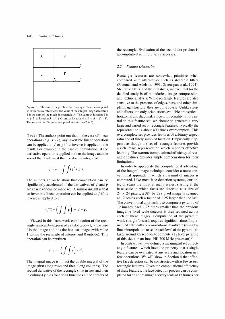
Figure 3. The sum of the pixels within rectangle D can be computedwith four array references. The value of the integral image at location1 is the sum of the pixels in rectangle A. The value at location 2 isA + B, at location 3 is A + C , and at location 4 is A + B + C + D.The sum within D can be computed as 4 + 1 − (2 + 3).

(1999). The authors point out that in the case of linearoperations (e.g. f · g), any invertible linear operationcan be applied to f or g if its inverse is applied to theresult. For example in the case of convolution, if thederivative operator is applied both to the image and thekernel the result must then be double integrated:

f ∗ g =∫ ∫

( f ′ ∗ g′).

The authors go on to show that convolution can besignificantly accelerated if the derivatives of f and gare sparse (or can be made so). A similar insight is thatan invertible linear operation can be applied to f if itsinverse is applied to g:

( f ′′) ∗( ∫ ∫

g

)= f ∗ g.

Viewed in this framework computation of the rect-angle sum can be expressed as a dot product, i ·r , wherei is the image and r is the box car image (with value1 within the rectangle of interest and 0 outside). Thisoperation can be rewritten

i · r =( ∫ ∫

i

)· r ′′.

The integral image is in fact the double integral of theimage (first along rows and then along columns). Thesecond derivative of the rectangle (first in row and thenin column) yields four delta functions at the corners of

the rectangle. Evaluation of the second dot product isaccomplished with four array accesses.

2.2. Feature Discussion

Rectangle features are somewhat primitive whencompared with alternatives such as steerable filters(Freeman and Adelson, 1991; Greenspan et al., 1994).Steerable filters, and their relatives, are excellent for thedetailed analysis of boundaries, image compression,and texture analysis. While rectangle features are alsosensitive to the presence of edges, bars, and other sim-ple image structure, they are quite coarse. Unlike steer-able filters, the only orientations available are vertical,horizontal and diagonal. Since orthogonality is not cen-tral to this feature set, we choose to generate a verylarge and varied set of rectangle features. Typically therepresentation is about 400 times overcomplete. Thisovercomplete set provides features of arbitrary aspectratio and of finely sampled location. Empirically it ap-pears as though the set of rectangle features providea rich image representation which supports effectivelearning. The extreme computational efficiency of rect-angle features provides ample compensation for theirlimitations.

In order to appreciate the computational advantageof the integral image technique, consider a more con-ventional approach in which a pyramid of images iscomputed. Like most face detection systems, our de-tector scans the input at many scales; starting at thebase scale in which faces are detected at a size of24 × 24 pixels, a 384 by 288 pixel image is scannedat 12 scales each a factor of 1.25 larger than the last.The conventional approach is to compute a pyramid of12 images, each 1.25 times smaller than the previousimage. A fixed scale detector is then scanned acrosseach of these images. Computation of the pyramid,while straightforward, requires significant time. Imple-mented efficiently on conventional hardware (using bi-linear interpolation to scale each level of the pyramid) ittakes around .05 seconds to compute a 12 level pyramidof this size (on an Intel PIII 700 MHz processor).5

In contrast we have defined a meaningful set of rect-angle features, which have the property that a singlefeature can be evaluated at any scale and location in afew operations. We will show in Section 4 that effec-tive face detectors can be constructed with as few as tworectangle features. Given the computational efficiencyof these features, the face detection process can be com-pleted for an entire image at every scale at 15 frames per


second, about the same time required to evaluate the 12level image pyramid alone. Any procedure which re-quires a pyramid of this type will necessarily run slowerthan our detector.

3. Learning Classification Functions

Given a feature set and a training set of positive andnegative images, any number of machine learning ap-proaches could be used to learn a classification func-tion. Sung and Poggio use a mixture of Gaussian model(Sung and Poggio, 1998). Rowley et al. (1998) use asmall set of simple image features and a neural net-work. Osuna et al. (1997b) used a support vector ma-chine. More recently Roth et al. (2000) have proposeda new and unusual image representation and have usedthe Winnow learning procedure.

Recall that there are 160,000 rectangle features as-sociated with each image sub-window, a number farlarger than the number of pixels. Even though eachfeature can be computed very efficiently, computingthe complete set is prohibitively expensive. Our hy-pothesis, which is borne out by experiment, is that avery small number of these features can be combinedto form an effective classifier. The main challenge is tofind these features.

In our system a variant of AdaBoost is used bothto select the features and to train the classifier (Freundand Schapire, 1995). In its original form, the AdaBoostlearning algorithm is used to boost the classificationperformance of a simple learning algorithm (e.g., itmight be used to boost the performance of a simple per-ceptron). It does this by combining a collection of weakclassification functions to form a stronger classifier. Inthe language of boosting the simple learning algorithmis called a weak learner. So, for example the percep-tron learning algorithm searches over the set of possibleperceptrons and returns the perceptron with the lowestclassification error. The learner is called weak becausewe do not expect even the best classification function toclassify the training data well (i.e. for a given problemthe best perceptron may only classify the training datacorrectly 51% of the time). In order for the weak learnerto be boosted, it is called upon to solve a sequence oflearning problems. After the first round of learning, theexamples are re-weighted in order to emphasize thosewhich were incorrectly classified by the previous weakclassifier. The final strong classifier takes the form of aperceptron, a weighted combination of weak classifiersfollowed by a threshold.6

The formal guarantees provided by the AdaBoostlearning procedure are quite strong. Freund andSchapire proved that the training error of the strongclassifier approaches zero exponentially in the numberof rounds. More importantly a number of resultswere later proved about generalization performance(Schapire et al., 1997). The key insight is that gen-eralization performance is related to the margin of theexamples, and that AdaBoost achieves large marginsrapidly.

The conventional AdaBoost procedure can be eas-ily interpreted as a greedy feature selection process.Consider the general problem of boosting, in which alarge set of classification functions are combined usinga weighted majority vote. The challenge is to associatea large weight with each good classification functionand a smaller weight with poor functions. AdaBoost isan aggressive mechanism for selecting a small set ofgood classification functions which nevertheless havesignificant variety. Drawing an analogy between weakclassifiers and features, AdaBoost is an effective pro-cedure for searching out a small number of good “fea-tures” which nevertheless have significant variety.

One practical method for completing this analogy isto restrict the weak learner to the set of classificationfunctions each of which depend on a single feature.In support of this goal, the weak learning algorithm isdesigned to select the single rectangle feature whichbest separates the positive and negative examples (thisis similar to the approach of Tieu and Viola (2000) inthe domain of image database retrieval). For each fea-ture, the weak learner determines the optimal thresholdclassification function, such that the minimum num-ber of examples are misclassified. A weak classifier(h(x, f, p, θ )) thus consists of a feature ( f ), a thresh-old (θ ) and a polarity (p) indicating the direction of theinequality:

h(x, f, p, θ ) ={

1 if p f (x) < pθ

0 otherwise

Here x is a 24 × 24 pixel sub-window of an image.In practice no single feature can perform the classifi-

cation task with low error. Features which are selectedearly in the process yield error rates between 0.1 and0.3. Features selected in later rounds, as the task be-comes more difficult, yield error rates between 0.4 and0.5. Table 1 shows the learning algorithm.

The weak classifiers that we use (thresholded singlefeatures) can be viewed as single node decision trees.

142 Viola and Jones

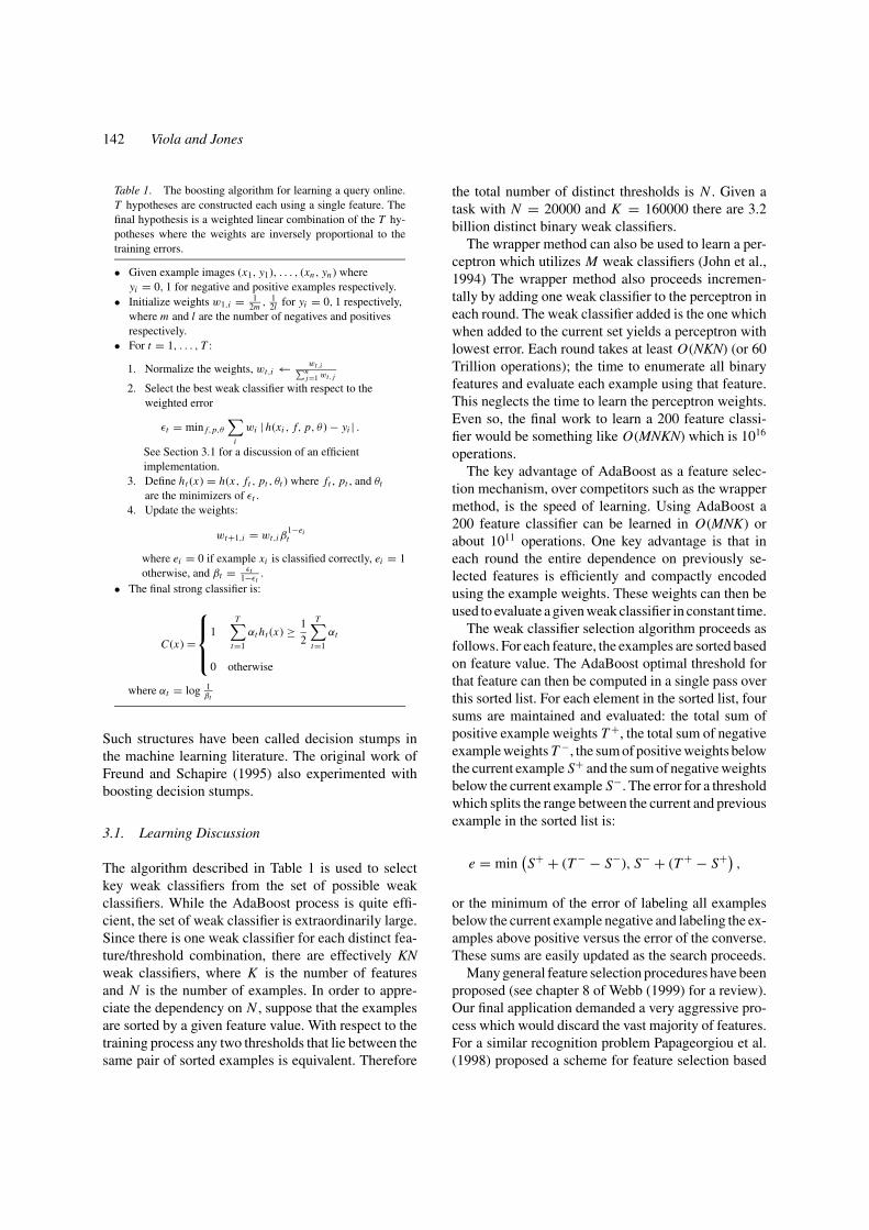
Table 1. The boosting algorithm for learning a query online.T hypotheses are constructed each using a single feature. Thefinal hypothesis is a weighted linear combination of the T hy-potheses where the weights are inversely proportional to thetraining errors.

• Given example images (x1, y1), . . . , (xn, yn) whereyi = 0, 1 for negative and positive examples respectively.

• Initialize weights w1,i = 12m , 1

2l for yi = 0, 1 respectively,where m and l are the number of negatives and positivesrespectively.

• For t = 1, . . . , T :

1. Normalize the weights, wt,i ← wt,i∑nj=1 wt, j

2. Select the best weak classifier with respect to theweighted error

εt = min f,p,θ

∑i

wi | h(xi , f, p, θ ) − yi | .See Section 3.1 for a discussion of an efficientimplementation.

3. Define ht (x) = h(x, ft , pt , θt ) where ft , pt , and θt

are the minimizers of εt .4. Update the weights:

wt+1,i = wt,i β1−eit

where ei = 0 if example xi is classified correctly, ei = 1otherwise, and βt = εt

1−εt.

• The final strong classifier is:

C(x) =

{1

T∑t=1

αt ht (x) ≥ 1

2

T∑t=1

αt

0 otherwise

where αt = log 1βt

Such structures have been called decision stumps inthe machine learning literature. The original work ofFreund and Schapire (1995) also experimented withboosting decision stumps.

3.1. Learning Discussion

The algorithm described in Table 1 is used to selectkey weak classifiers from the set of possible weakclassifiers. While the AdaBoost process is quite effi-cient, the set of weak classifier is extraordinarily large.Since there is one weak classifier for each distinct fea-ture/threshold combination, there are effectively KNweak classifiers, where K is the number of featuresand N is the number of examples. In order to appre-ciate the dependency on N , suppose that the examplesare sorted by a given feature value. With respect to thetraining process any two thresholds that lie between thesame pair of sorted examples is equivalent. Therefore

the total number of distinct thresholds is N . Given atask with N = 20000 and K = 160000 there are 3.2billion distinct binary weak classifiers.

The wrapper method can also be used to learn a per-ceptron which utilizes M weak classifiers (John et al.,1994) The wrapper method also proceeds incremen-tally by adding one weak classifier to the perceptron ineach round. The weak classifier added is the one whichwhen added to the current set yields a perceptron withlowest error. Each round takes at least O(NKN) (or 60Trillion operations); the time to enumerate all binaryfeatures and evaluate each example using that feature.This neglects the time to learn the perceptron weights.Even so, the final work to learn a 200 feature classi-fier would be something like O(MNKN) which is 1016

operations.The key advantage of AdaBoost as a feature selec-

tion mechanism, over competitors such as the wrappermethod, is the speed of learning. Using AdaBoost a200 feature classifier can be learned in O(MNK) orabout 1011 operations. One key advantage is that ineach round the entire dependence on previously se-lected features is efficiently and compactly encodedusing the example weights. These weights can then beused to evaluate a given weak classifier in constant time.

The weak classifier selection algorithm proceeds asfollows. For each feature, the examples are sorted basedon feature value. The AdaBoost optimal threshold forthat feature can then be computed in a single pass overthis sorted list. For each element in the sorted list, foursums are maintained and evaluated: the total sum ofpositive example weights T +, the total sum of negativeexample weights T −, the sum of positive weights belowthe current example S+ and the sum of negative weightsbelow the current example S−. The error for a thresholdwhich splits the range between the current and previousexample in the sorted list is:

e = min(S+ + (T − − S−), S− + (T + − S+)

,

or the minimum of the error of labeling all examplesbelow the current example negative and labeling the ex-amples above positive versus the error of the converse.These sums are easily updated as the search proceeds.

Many general feature selection procedures have beenproposed (see chapter 8 of Webb (1999) for a review).Our final application demanded a very aggressive pro-cess which would discard the vast majority of features.For a similar recognition problem Papageorgiou et al.(1998) proposed a scheme for feature selection based


on feature variance. They demonstrated good results se-lecting 37 features out of a total 1734 features. Whilethis is a significant reduction, the number of featuresevaluated for every image sub-window is still reason-ably large.

Roth et al. (2000) propose a feature selection processbased on the Winnow exponential perceptron learningrule. These authors use a very large and unusual featureset, where each pixel is mapped into a binary vector of ddimensions (when a particular pixel takes on the valuex , in the range [0, d − 1], the x-th dimension is set to1 and the other dimensions to 0). The binary vectorsfor each pixel are concatenated to form a single binaryvector with nd dimensions (n is the number of pixels).The classification rule is a perceptron, which assignsone weight to each dimension of the input vector. TheWinnow learning process converges to a solution wheremany of these weights are zero. Nevertheless a verylarge number of features are retained (perhaps a fewhundred or thousand).

3.2. Learning Results

While details on the training and performance of thefinal system are presented in Section 5, several sim-ple results merit discussion. Initial experiments demon-

Figure 4. Receiver operating characteristic (ROC) curve for the 200 feature classifier.

strated that a classifier constructed from 200 featureswould yield reasonable results (see Fig. 4). Given adetection rate of 95% the classifier yielded a false pos-itive rate of 1 in 14084 on a testing dataset. This ispromising, but for a face detector to be practical forreal applications, the false positive rate must be closerto 1 in 1,000,000.

For the task of face detection, the initial rectanglefeatures selected by AdaBoost are meaningful and eas-ily interpreted. The first feature selected seems to focuson the property that the region of the eyes is often darkerthan the region of the nose and cheeks (see Fig. 5). Thisfeature is relatively large in comparison with the detec-tion sub-window, and should be somewhat insensitiveto size and location of the face. The second feature se-lected relies on the property that the eyes are darkerthan the bridge of the nose.

In summary the 200-feature classifier provides ini-tial evidence that a boosted classifier constructed fromrectangle features is an effective technique for face de-tection. In terms of detection, these results are com-pelling but not sufficient for many real-world tasks. Interms of computation, this classifier is very fast, re-quiring 0.7 seconds to scan an 384 by 288 pixel im-age. Unfortunately, the most straightforward tech-nique for improving detection performance, adding

144 Viola and Jones

Figure 5. The first and second features selected by AdaBoost. Thetwo features are shown in the top row and then overlayed on a typ-ical training face in the bottom row. The first feature measures thedifference in intensity between the region of the eyes and a regionacross the upper cheeks. The feature capitalizes on the observationthat the eye region is often darker than the cheeks. The second featurecompares the intensities in the eye regions to the intensity across thebridge of the nose.

features to the classifier, directly increases computationtime.

4. The Attentional Cascade

This section describes an algorithm for constructing acascade of classifiers which achieves increased detec-tion performance while radically reducing computationtime. The key insight is that smaller, and therefore moreefficient, boosted classifiers can be constructed whichreject many of the negative sub-windows while detect-ing almost all positive instances. Simpler classifiers areused to reject the majority of sub-windows before morecomplex classifiers are called upon to achieve low falsepositive rates.

Stages in the cascade are constructed by trainingclassifiers using AdaBoost. Starting with a two-featurestrong classifier, an effective face filter can be obtainedby adjusting the strong classifier threshold to mini-mize false negatives. The initial AdaBoost threshold,12

∑Tt=1 αt , is designed to yield a low error rate on the

training data. A lower threshold yields higher detec-tion rates and higher false positive rates. Based on per-formance measured using a validation training set, thetwo-feature classifier can be adjusted to detect 100% ofthe faces with a false positive rate of 50%. See Fig. 5 fora description of the two features used in this classifier.

The detection performance of the two-feature clas-sifier is far from acceptable as a face detection system.Nevertheless the classifier can significantly reduce the

number of sub-windows that need further processingwith very few operations:

1. Evaluate the rectangle features (requires between 6and 9 array references per feature).

2. Compute the weak classifier for each feature (re-quires one threshold operation per feature).

3. Combine the weak classifiers (requires one multiplyper feature, an addition, and finally a threshold).

A two feature classifier amounts to about 60 mi-croprocessor instructions. It seems hard to imaginethat any simpler filter could achieve higher rejectionrates. By comparison, scanning a simple image tem-plate would require at least 20 times as many operationsper sub-window.

The overall form of the detection process is that ofa degenerate decision tree, what we call a “cascade”(Quinlan, 1986) (see Fig. 6). A positive result fromthe first classifier triggers the evaluation of a secondclassifier which has also been adjusted to achieve veryhigh detection rates. A positive result from the secondclassifier triggers a third classifier, and so on. A negativeoutcome at any point leads to the immediate rejectionof the sub-window.

The structure of the cascade reflects the fact thatwithin any single image an overwhelming majority ofsub-windows are negative. As such, the cascade at-tempts to reject as many negatives as possible at theearliest stage possible. While a positive instance will

Figure 6. Schematic depiction of a the detection cascade. A seriesof classifiers are applied to every sub-window. The initial classifiereliminates a large number of negative examples with very little pro-cessing. Subsequent layers eliminate additional negatives but requireadditional computation. After several stages of processing the num-ber of sub-windows have been reduced radically. Further processingcan take any form such as additional stages of the cascade (as in ourdetection system) or an alternative detection system.


trigger the evaluation of every classifier in the cascade,this is an exceedingly rare event.

Much like a decision tree, subsequent classifiers aretrained using those examples which pass through allthe previous stages. As a result, the second classifierfaces a more difficult task than the first. The exampleswhich make it through the first stage are “harder” thantypical examples. The more difficult examples facedby deeper classifiers push the entire receiver operat-ing characteristic (ROC) curve downward. At a givendetection rate, deeper classifiers have correspondinglyhigher false positive rates.

4.1. Training a Cascade of Classifiers

The cascade design process is driven from a set of de-tection and performance goals. For the face detectiontask, past systems have achieved good detection rates(between 85 and 95 percent) and extremely low falsepositive rates (on the order of 10−5 or 10−6). The num-ber of cascade stages and the size of each stage mustbe sufficient to achieve similar detection performancewhile minimizing computation.

Given a trained cascade of classifiers, the false pos-itive rate of the cascade is

F =K∏

i=1

fi ,

where F is the false positive rate of the cascaded clas-sifier, K is the number of classifiers, and fi is the falsepositive rate of the i th classifier on the examples thatget through to it. The detection rate is

D =K∏

i=1

di ,

where D is the detection rate of the cascaded classifier,K is the number of classifiers, and di is the detectionrate of the i th classifier on the examples that get throughto it.

Given concrete goals for overall false positive anddetection rates, target rates can be determined for eachstage in the cascade process. For example a detectionrate of 0.9 can be achieved by a 10 stage classifier ifeach stage has a detection rate of 0.99 (since 0.9 ≈0.9910). While achieving this detection rate may soundlike a daunting task, it is made significantly easier by thefact that each stage need only achieve a false positiverate of about 30% (0.3010 ≈ 6 × 10−6).

The number of features evaluated when scanningreal images is necessarily a probabilistic process. Anygiven sub-window will progress down through the cas-cade, one classifier at a time, until it is decided thatthe window is negative or, in rare circumstances, thewindow succeeds in each test and is labelled positive.The expected behavior of this process is determinedby the distribution of image windows in a typical testset. The key measure of each classifier is its “positiverate”, the proportion of windows which are labelled aspotentially containing a face. The expected number offeatures which are evaluated is:

N = n0 +K∑

i=1

(ni

∏j<i

p j

)

where N is the expected number of features evaluated,K is the number of classifiers, pi is the positive rate ofthe i th classifier, and ni are the number of features in thei th classifier. Interestingly, since faces are extremelyrare, the “positive rate” is effectively equal to the falsepositive rate.

The process by which each element of the cascadeis trained requires some care. The AdaBoost learningprocedure presented in Section 3 attempts only to min-imize errors, and is not specifically designed to achievehigh detection rates at the expense of large false positiverates. One simple, and very conventional, scheme fortrading off these errors is to adjust the threshold of theperceptron produced by AdaBoost. Higher thresholdsyield classifiers with fewer false positives and a lowerdetection rate. Lower thresholds yield classifiers withmore false positives and a higher detection rate. It isnot clear, at this point, whether adjusting the thresholdin this way preserves the training and generalizationguarantees provided by AdaBoost.

The overall training process involves two types oftradeoffs. In most cases classifiers with more featureswill achieve higher detection rates and lower false pos-itive rates. At the same time classifiers with more fea-tures require more time to compute. In principle onecould define an optimization framework in which

• the number of classifier stages,• the number of features, ni , of each stage,• the threshold of each stage

are traded off in order to minimize the expected num-ber of features N given a target for F and D. Unfortu-nately finding this optimum is a tremendously difficultproblem.

146 Viola and Jones

Table 2. The training algorithm for building a cascaded detector.

• User selects values for f , the maximum acceptable falsepositive rate per layer and d, the minimum acceptable detectionrate per layer.

• User selects target overall false positive rate, Ftarget .• P = set of positive examples• N = set of negative examples• F0 = 1.0; D0 = 1.0• i = 0• while Fi > Ftarget

– i ← i + 1– ni = 0; Fi = Fi−1

– while Fi > f × Fi−1

∗ ni ← ni + 1∗ Use P and N to train a classifier with ni features using

AdaBoost∗ Evaluate current cascaded classifier on validation set to

determine Fi and Di .∗ Decrease threshold for the i th classifier until the current

cascaded classifier has a detection rate of at leastd × Di−1 (this also affects Fi )

– N ← ∅– If Fi > Ftarget then evaluate the current cascaded detector on

the set of non-face images and put any false detections intothe set N

In practice a very simple framework is used to pro-duce an effective classifier which is highly efficient.The user selects the maximum acceptable rate for fi

and the minimum acceptable rate for di . Each layer ofthe cascade is trained by AdaBoost (as described inTable 1) with the number of features used being in-creased until the target detection and false positive ratesare met for this level. The rates are determined by test-ing the current detector on a validation set. If the overalltarget false positive rate is not yet met then another layeris added to the cascade. The negative set for trainingsubsequent layers is obtained by collecting all false de-tections found by running the current detector on a setof images which do not contain any instances of faces.This algorithm is given more precisely in Table 2.

4.2. Simple Experiment

In order to explore the feasibility of the cascade ap-proach two simple detectors were trained: a mono-lithic 200-feature classifier and a cascade of ten20-feature classifiers. The first stage classifier in thecascade was trained using 5000 faces and 10000 non-face sub-windows randomly chosen from non-face im-ages. The second stage classifier was trained on the

same 5000 faces plus 5000 false positives of the firstclassifier. This process continued so that subsequentstages were trained using the false positives of the pre-vious stage.

The monolithic 200-feature classifier was trained onthe union of all examples used to train all the stagesof the cascaded classifier. Note that without referenceto the cascaded classifier, it might be difficult to se-lect a set of non-face training examples to train themonolithic classifier. We could of course use all possi-ble sub-windows from all of our non-face images, butthis would make the training time impractically long.The sequential way in which the cascaded classifier istrained effectively reduces the non-face training set bythrowing out easy examples and focusing on the “hard”ones.

Figure 7 gives the ROC curves comparing the per-formance of the two classifiers. It shows that there islittle difference between the two in terms of accuracy.However, there is a big difference in terms of speed.The cascaded classifier is nearly 10 times faster sinceits first stage throws out most non-faces so that they arenever evaluated by subsequent stages.

4.3. Detector Cascade Discussion

There is a hidden benefit of training a detector as a se-quence of classifiers which is that the effective numberof negative examples that the final detector sees can bevery large. One can imagine training a single large clas-sifier with many features and then trying to speed upits running time by looking at partial sums of featuresand stopping the computation early if a partial sum isbelow the appropriate threshold. One drawback of suchan approach is that the training set of negative exam-ples would have to be relatively small (on the order of10,000 to maybe 100,000 examples) to make trainingfeasible. With the cascaded detector, the final layers ofthe cascade may effectively look through hundreds ofmillions of negative examples in order to find a set of10,000 negative examples that the earlier layers of thecascade fail on. So the negative training set is muchlarger and more focused on the hard examples for acascaded detector.

A notion similar to the cascade appears in the facedetection system described by Rowley et al. (1998).Rowley et al. trained two neural networks. One networkwas moderately complex, focused on a small region ofthe image, and detected faces with a low false positiverate. They also trained a second neural network which


Figure 7. ROC curves comparing a 200-feature classifier with a cascaded classifier containing ten 20-feature classifiers. Accuracy is notsignificantly different, but the speed of the cascaded classifier is almost 10 times faster.

was much faster, focused on a larger regions of theimage, and detected faces with a higher false positiverate. Rowley et al. used the faster second network toprescreen the image in order to find candidate regionsfor the slower more accurate network. Though it isdifficult to determine exactly, it appears that Rowleyet al.’s two network face system is the fastest existingface detector.7 Our system uses a similar approach, butit extends this two stage cascade to include 38 stages.

The structure of the cascaded detection process isessentially that of a degenerate decision tree, and assuch is related to the work of Amit and Geman (1999).Unlike techniques which use a fixed detector, Amit andGeman propose an alternative point of view where un-usual co-occurrences of simple image features are usedto trigger the evaluation of a more complex detectionprocess. In this way the full detection process need notbe evaluated at many of the potential image locationsand scales. While this basic insight is very valuable,in their implementation it is necessary to first evaluatesome feature detector at every location. These featuresare then grouped to find unusual co-occurrences. Inpractice, since the form of our detector and the fea-tures that it uses are extremely efficient, the amortizedcost of evaluating our detector at every scale and lo-

cation is much faster than finding and grouping edgesthroughout the image.

In recent work Fleuret and Geman (2001) have pre-sented a face detection technique which relies on a“chain” of tests in order to signify the presence of aface at a particular scale and location. The image prop-erties measured by Fleuret and Geman, disjunctionsof fine scale edges, are quite different than rectanglefeatures which are simple, exist at all scales, and aresomewhat interpretable. The two approaches also differradically in their learning philosophy. Because Fleuretand Geman’s learning process does not use negativeexamples their approach is based more on density es-timation, while our detector is purely discriminative.Finally the false positive rate of Fleuret and Geman’sapproach appears to be higher than that of previous ap-proaches like Rowley et al. and this approach. In thepublished paper the included example images each hadbetween 2 and 10 false positives. For many practicaltasks, it is important that the expected number of falsepositives in any image be less than one (since in manytasks the expected number of true positives is less thanone as well). Unfortunately the paper does not reportquantitative detection and false positive results on stan-dard datasets.

148 Viola and Jones

5. Results

This section describes the final face detection system.The discussion includes details on the structure andtraining of the cascaded detector as well as results ona large real-world testing set.

5.1. Training Dataset

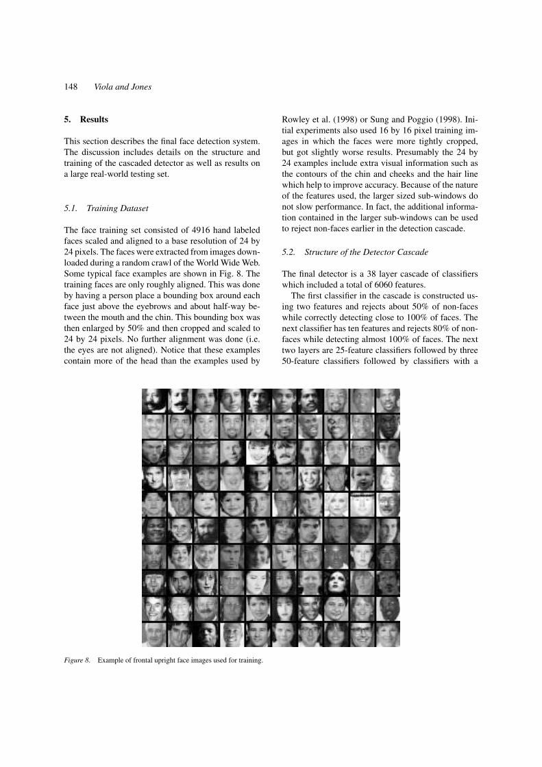
The face training set consisted of 4916 hand labeledfaces scaled and aligned to a base resolution of 24 by24 pixels. The faces were extracted from images down-loaded during a random crawl of the World Wide Web.Some typical face examples are shown in Fig. 8. Thetraining faces are only roughly aligned. This was doneby having a person place a bounding box around eachface just above the eyebrows and about half-way be-tween the mouth and the chin. This bounding box wasthen enlarged by 50% and then cropped and scaled to24 by 24 pixels. No further alignment was done (i.e.the eyes are not aligned). Notice that these examplescontain more of the head than the examples used by

Figure 8. Example of frontal upright face images used for training.

Rowley et al. (1998) or Sung and Poggio (1998). Ini-tial experiments also used 16 by 16 pixel training im-ages in which the faces were more tightly cropped,but got slightly worse results. Presumably the 24 by24 examples include extra visual information such asthe contours of the chin and cheeks and the hair linewhich help to improve accuracy. Because of the natureof the features used, the larger sized sub-windows donot slow performance. In fact, the additional informa-tion contained in the larger sub-windows can be usedto reject non-faces earlier in the detection cascade.

5.2. Structure of the Detector Cascade

The final detector is a 38 layer cascade of classifierswhich included a total of 6060 features.

The first classifier in the cascade is constructed us-ing two features and rejects about 50% of non-faceswhile correctly detecting close to 100% of faces. Thenext classifier has ten features and rejects 80% of non-faces while detecting almost 100% of faces. The nexttwo layers are 25-feature classifiers followed by three50-feature classifiers followed by classifiers with a


variety of different numbers of features chosen accord-ing to the algorithm in Table 2. The particular choicesof number of features per layer was driven througha trial and error process in which the number of fea-tures were increased until a significant reduction in thefalse positive rate could be achieved. More levels wereadded until the false positive rate on the validation setwas nearly zero while still maintaining a high correctdetection rate. The final number of layers, and the sizeof each layer, are not critical to the final system perfor-mance. The procedure we used to choose the numberof features per layer was guided by human intervention(for the first 7 layers) in order to reduce the training timefor the detector. The algorithm described in Table 2 wasmodified slightly to ease the computational burden byspecifying a minimum number of features per layer byhand and by adding more than 1 feature at a time. Inlater layers, 25 features were added at a time beforetesting on the validation set. This avoided having totest the detector on the validation set for every singlefeature added to a classifier.

The non-face sub-windows used to train the firstlevel of the cascade were collected by selecting ran-dom sub-windows from a set of 9500 images whichdid not contain faces. The non-face examples used totrain subsequent layers were obtained by scanning thepartial cascade across large non-face images and col-lecting false positives. A maximum of 6000 such non-face sub-windows were collected for each layer. Thereare approximately 350 million non-face sub-windowscontained in the 9500 non-face images.

Training time for the entire 38 layer detector was onthe order of weeks on a single 466 MHz AlphaStationXP900. We have since parallelized the algorithm tomake it possible to train a complete cascade in about aday.

5.3. Speed of the Final Detector

The speed of the cascaded detector is directly relatedto the number of features evaluated per scanned sub-window. As discussed in Section 4.1, the number of fea-tures evaluated depends on the images being scanned.Since a large majority of the sub-windows are dis-carded by the first two stages of the cascade, an av-erage of 8 features out of a total of 6060 are eval-uated per sub-window (as evaluated on the MIT +CMU (Rowley et al., 1998). On a 700 Mhz PentiumIII processor, the face detector can process a 384 by288 pixel image in about .067 seconds (using a starting

scale of 1.25 and a step size of 1.5 described below).This is roughly 15 times faster than the Rowley-Baluja-Kanade detector (Rowley et al., 1998) and about 600times faster than the Schneiderman-Kanade detector(Schneiderman and Kanade, 2000).

5.4. Image Processing

All example sub-windows used for training were vari-ance normalized to minimize the effect of differentlighting conditions. Normalization is therefore neces-sary during detection as well. The variance of an imagesub-window can be computed quickly using a pair ofintegral images. Recall that σ 2 = m2 − 1

N

∑x2, where

σ is the standard deviation, m is the mean, and x isthe pixel value within the sub-window. The mean of asub-window can be computed using the integral image.The sum of squared pixels is computed using an integralimage of the image squared (i.e. two integral imagesare used in the scanning process). During scanning theeffect of image normalization can be achieved by postmultiplying the feature values rather than operating onthe pixels.

5.5. Scanning the Detector

The final detector is scanned across the image at multi-ple scales and locations. Scaling is achieved by scalingthe detector itself, rather than scaling the image. Thisprocess makes sense because the features can be eval-uated at any scale with the same cost. Good detectionresults were obtained using scales which are a factor of1.25 apart.

The detector is also scanned across location. Sub-sequent locations are obtained by shifting the windowsome number of pixels �. This shifting process is af-fected by the scale of the detector: if the current scale iss the window is shifted by [s�], where [] is the round-ing operation.

The choice of � affects both the speed of the de-tector as well as accuracy. Since the training imageshave some translational variability the learned detectorachieves good detection performance in spite of smallshifts in the image. As a result the detector sub-windowcan be shifted more than one pixel at a time. However,a step size of more than one pixel tends to decrease thedetection rate slightly while also decreasing the numberof false positives. We present results for two differentstep sizes.

150 Viola and Jones

5.6. Integration of Multiple Detections

Since the final detector is insensitive to small changesin translation and scale, multiple detections will usuallyoccur around each face in a scanned image. The sameis often true of some types of false positives. In practiceit often makes sense to return one final detection perface. Toward this end it is useful to postprocess thedetected sub-windows in order to combine overlappingdetections into a single detection.

In these experiments detections are combined in avery simple fashion. The set of detections are first par-titioned into disjoint subsets. Two detections are in thesame subset if their bounding regions overlap. Eachpartition yields a single final detection. The corners ofthe final bounding region are the average of the cornersof all detections in the set.

In some cases this postprocessing decreases the num-ber of false positives since an overlapping subset offalse positives is reduced to a single detection.

5.7. Experiments on a Real-World Test Set

We tested our system on the MIT + CMU frontal facetest set (Rowley et al., 1998). This set consists of 130

Figure 9. ROC curves for our face detector on the MIT + CMU test set. The detector was run once using a step size of 1.0 and starting scaleof 1.0 (75,081,800 sub-windows scanned) and then again using a step size of 1.5 and starting scale of 1.25 (18,901,947 sub-windows scanned).In both cases a scale factor of 1.25 was used.

images with 507 labeled frontal faces. A ROC curveshowing the performance of our detector on this testset is shown in Fig. 9. To create the ROC curve thethreshold of the perceptron on the final layer classifieris adjusted from +∞ to −∞. Adjusting the threshold to+∞ will yield a detection rate of 0.0 and a false positiverate of 0.0. Adjusting the threshold to −∞, however,increases both the detection rate and false positive rate,but only to a certain point. Neither rate can be higherthan the rate of the detection cascade minus the finallayer. In effect, a threshold of −∞ is equivalent to re-moving that layer. Further increasing the detection andfalse positive rates requires decreasing the thresholdof the next classifier in the cascade. Thus, in order toconstruct a complete ROC curve, classifier layers areremoved. We use the number of false positives as op-posed to the rate of false positives for the x-axis ofthe ROC curve to facilitate comparison with other sys-tems. To compute the false positive rate, simply divideby the total number of sub-windows scanned. For thecase of � = 1.0 and starting scale = 1.0, the numberof sub-windows scanned is 75,081,800. For � = 1.5and starting scale = 1.25, the number of sub-windowsscanned is 18,901,947.

Unfortunately, most previous published results onface detection have only included a single operating


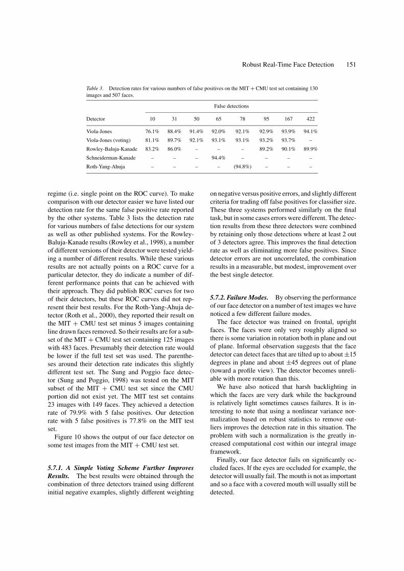
Table 3. Detection rates for various numbers of false positives on the MIT + CMU test set containing 130images and 507 faces.

False detections

Detector 10 31 50 65 78 95 167 422

Viola-Jones 76.1% 88.4% 91.4% 92.0% 92.1% 92.9% 93.9% 94.1%

Viola-Jones (voting) 81.1% 89.7% 92.1% 93.1% 93.1% 93.2% 93.7% –

Rowley-Baluja-Kanade 83.2% 86.0% – – – 89.2% 90.1% 89.9%

Schneiderman-Kanade – – – 94.4% – – – –

Roth-Yang-Ahuja – – – – (94.8%) – – –

regime (i.e. single point on the ROC curve). To makecomparison with our detector easier we have listed ourdetection rate for the same false positive rate reportedby the other systems. Table 3 lists the detection ratefor various numbers of false detections for our systemas well as other published systems. For the Rowley-Baluja-Kanade results (Rowley et al., 1998), a numberof different versions of their detector were tested yield-ing a number of different results. While these variousresults are not actually points on a ROC curve for aparticular detector, they do indicate a number of dif-ferent performance points that can be achieved withtheir approach. They did publish ROC curves for twoof their detectors, but these ROC curves did not rep-resent their best results. For the Roth-Yang-Ahuja de-tector (Roth et al., 2000), they reported their result onthe MIT + CMU test set minus 5 images containingline drawn faces removed. So their results are for a sub-set of the MIT + CMU test set containing 125 imageswith 483 faces. Presumably their detection rate wouldbe lower if the full test set was used. The parenthe-ses around their detection rate indicates this slightlydifferent test set. The Sung and Poggio face detec-tor (Sung and Poggio, 1998) was tested on the MITsubset of the MIT + CMU test set since the CMUportion did not exist yet. The MIT test set contains23 images with 149 faces. They achieved a detectionrate of 79.9% with 5 false positives. Our detectionrate with 5 false positives is 77.8% on the MIT testset.

Figure 10 shows the output of our face detector onsome test images from the MIT + CMU test set.

5.7.1. A Simple Voting Scheme Further ImprovesResults. The best results were obtained through thecombination of three detectors trained using differentinitial negative examples, slightly different weighting

on negative versus positive errors, and slightly differentcriteria for trading off false positives for classifier size.These three systems performed similarly on the finaltask, but in some cases errors were different. The detec-tion results from these three detectors were combinedby retaining only those detections where at least 2 outof 3 detectors agree. This improves the final detectionrate as well as eliminating more false positives. Sincedetector errors are not uncorrelated, the combinationresults in a measurable, but modest, improvement overthe best single detector.

5.7.2. Failure Modes. By observing the performanceof our face detector on a number of test images we havenoticed a few different failure modes.

The face detector was trained on frontal, uprightfaces. The faces were only very roughly aligned sothere is some variation in rotation both in plane and outof plane. Informal observation suggests that the facedetector can detect faces that are tilted up to about ±15degrees in plane and about ±45 degrees out of plane(toward a profile view). The detector becomes unreli-able with more rotation than this.

We have also noticed that harsh backlighting inwhich the faces are very dark while the backgroundis relatively light sometimes causes failures. It is in-teresting to note that using a nonlinear variance nor-malization based on robust statistics to remove out-liers improves the detection rate in this situation. Theproblem with such a normalization is the greatly in-creased computational cost within our integral imageframework.

Finally, our face detector fails on significantly oc-cluded faces. If the eyes are occluded for example, thedetector will usually fail. The mouth is not as importantand so a face with a covered mouth will usually still bedetected.

152 Viola and Jones

Figure 10. Output of our face detector on a number of test images from the MIT + CMU test set.

6. Conclusions

We have presented an approach for face detectionwhich minimizes computation time while achievinghigh detection accuracy. The approach was used to con-struct a face detection system which is approximately15 times faster than any previous approach. Preliminaryexperiments, which will be described elsewhere, showthat highly efficient detectors for other objects, such aspedestrians or automobiles, can also be constructed inthis way.

This paper brings together new algorithms, represen-tations, and insights which are quite generic and maywell have broader application in computer vision andimage processing.

The first contribution is a new a technique for com-puting a rich set of image features using the integralimage. In order to achieve true scale invariance, almostall face detection systems must operate on multipleimage scales. The integral image, by eliminating theneed to compute a multi-scale image pyramid, reducesthe initial image processing required for face detection


significantly. Using the integral image, face detectionis completed in almost the same time as it takes for animage pyramid to be computed.

While the integral image should also have immedi-ate use for other systems which have used Haar-likefeatures such as Papageorgiou et al. (1998), it can fore-seeably have impact on any task where Haar-like fea-tures may be of value. Initial experiments have shownthat a similar feature set is also effective for the taskof parameter estimation, where the expression of aface, the position of a head, or the pose of an object isdetermined.

The second contribution of this paper is a simpleand efficient classifier built from computationally ef-ficient features using AdaBoost for feature selection.This classifier is clearly an effective one for face detec-tion and we are confident that it will also be effective inother domains such as automobile or pedestrian detec-tion. Furthermore, the idea of an aggressive and effec-tive technique for feature selection should have impacton a wide variety of learning tasks. Given an effectivetool for feature selection, the system designer is free todefine a very large and very complex set of features asinput for the learning process. The resulting classifieris nevertheless computationally efficient, since only asmall number of features need to be evaluated duringrun time. Frequently the resulting classifier is also quitesimple; within a large set of complex features it is morelikely that a few critical features can be found whichcapture the structure of the classification problem in astraightforward fashion.

The third contribution of this paper is a technique forconstructing a cascade of classifiers which radicallyreduces computation time while improving detectionaccuracy. Early stages of the cascade are designed toreject a majority of the image in order to focus subse-quent processing on promising regions. One key pointis that the cascade presented is quite simple and ho-mogeneous in structure. Previous approaches for at-tentive filtering, such as Itti et al. (1998) propose amore complex and heterogeneous mechanism for fil-tering. Similarly Amit and Geman (1999) propose ahierarchical structure for detection in which the stagesare quite different in structure and processing. A ho-mogeneous system, besides being easy to implementand understand, has the advantage that simple tradeoffscan be made between processing time and detectionperformance.

Finally this paper presents a set of detailed exper-iments on a difficult face detection dataset which has

been widely studied. This dataset includes faces undera very wide range of conditions including: illumina-tion, scale, pose, and camera variation. Experiments onsuch a large and complex dataset are difficult and timeconsuming. Nevertheless systems which work underthese conditions are unlikely to be brittle or limited to asingle set of conditions. More importantly conclusionsdrawn from this dataset are unlikely to be experimentalartifacts.

Acknowledgments

The authors would like to thank T.M. Murali, Jim Rehg,Tat-Jen Cham, Rahul Sukthankar, Vladimir Pavlovic,and Thomas Leung for the their helpful comments.Henry Rowley was extremely helpful in providing im-plementations of his face detector for comparison withour own.

Notes

1. Supervised refers to the fact that the attentional operator is trainedto detect examples of a particular class.

2. Henry Rowley very graciously supplied us with implementationsof his detection system for direct comparison. Reported resultsare against his fastest system. It is difficult to determine fromthe published literature, but the Rowley-Baluja-Kanade detectoris widely considered the fastest detection system and has beenheavily tested on real-world problems.

3. A complete basis has no linear dependence between basis ele-ments and has the same number of elements as the image space,in this case 576. The full set of 160,000 features is many timesover-complete.

4. There is a close relation to “summed area tables” as used in graph-ics (Crow, 1984). We choose a different name here in order to em-phasize its use for the analysis of images, rather than for texturemapping.

5. The availability of custom hardware and the appearance of spe-cial instruction sets like Intel MMX can change this analysis.It is nevertheless instructive to compare performance assumingconventional software algorithms.

6. In the case where the weak learner is a perceptron learning al-gorithm, the final boosted classifier is a two layer perceptron. Atwo layer perceptron is in principle much more powerful than anysingle layer perceptron.

7. Among other published face detection systems some are poten-tially faster. These have either neglected to discuss performancein detail, or have never published detection and false positive rateson a large and difficult training set.

References

Amit, Y. and Geman, D. 1999. A computational model for visualselection. Neural Computation, 11:1691–1715.

154 Viola and Jones

Crow, F. 1984. Summed-area tables for texture mapping. In Proceed-ings of SIGGRAPH, 18(3):207–212.

Fleuret, F. and Geman, D. 2001. Coarse-to-fine face detection. Int.J. Computer Vision, 41:85–107.

Freeman, W.T. and Adelson, E.H. 1991. The design and use of steer-able filters. IEEE Transactions on Pattern Analysis and MachineIntelligence, 13(9):891–906.

Freund, Y. and Schapire, R.E. 1995. A decision-theoretic generaliza-tion of on-line learning and an application to boosting. In Com-putational Learning Theory: Eurocolt 95, Springer-Verlag, pp.23–37.

Greenspan, H., Belongie, S., Gooodman, R., Perona, P., Rakshit, S.,and Anderson, C. 1994. Overcomplete steerable pyramid filtersand rotation invariance. In Proceedings of the IEEE Conferenceon Computer Vision and Pattern Recognition.

Itti, L., Koch, C., and Niebur, E. 1998. A model of saliency-basedvisual attention for rapid scene analysis. IEEE Patt. Anal. Mach.Intell., 20(11):1254-–1259.

John, G., Kohavi, R., and Pfeger, K. 1994. Irrelevant features andthe subset selection problem. In Machine Learning ConferenceProceedings.

Osuna, E., Freund, R., and Girosi, F. 1997a. Training supportvector machines: An application to face detection. In Proceed-ings of the IEEE Conference on Computer Vision and PatternRecognition.

Osuna, E., Freund, R., and Girosi, F. 1997b. Training support vectormachines: an application to face detection. In Proceedings of theIEEE Conference on Computer Vision and Pattern Recognition.

Papageorgiou, C., Oren, M., and Poggio, T. 1998. A general frame-work for object detection. In International Conference on Com-puter Vision.

Quinlan, J. 1986. Induction of decision trees. Machine Learning,1:81–106.

Roth, D., Yang, M., and Ahuja, N. 2000. A snowbased face detector.In Neural Information Processing 12.

Rowley, H., Baluja, S., and Kanade, T. 1998. Neural network-basedface detection. IEEE Patt. Anal. Mach. Intell., 20:22–38.

Schapire, R.E., Freund, Y., Bartlett, P., and Lee, W.S. 1997. Boost-ing the margin: A new explanation for the effectiveness of votingmethods. In Proceedings of the Fourteenth International Confer-ence on Machine Learning.

Schapire, R.E., Freund, Y., Bartlett, P., and Lee, W.S. 1998. Boost-ing the margin: A new explanation for the effectiveness of votingmethods. Ann. Stat., 26(5):1651–1686.

Schneiderman, H. and Kanade, T. 2000. A statistical method for3D object detection applied to faces and cars. In InternationalConference on Computer Vision.

Simard, P.Y., Bottou, L., Haffner, P., and LeCun, Y. (1999). Boxlets:A fast convolution algorithm for signal processing and neural net-works. In M. Kearns, S. Solla, and D. Cohn (Eds.), Advancesin Neural Information Processing Systems, vol. 11, pp. 571–577.

Sung, K. and Poggio, T. 1998. Example-based learning for view-based face detection. IEEE Patt. Anal. Mach. Intell., 20:39–51.

Tieu, K. and Viola, P. 2000. Boosting image retrieval. In Proceedingsof the IEEE Conference on Computer Vision and Pattern Recog-nition.

Tsotsos, J., Culhane, S., Wai, W., Lai, Y., Davis, N., and Nuflo,F. 1995. Modeling visual-attention via selective tuning. ArtificialIntelligence Journal, 78(1/2):507–545.

Webb, A. 1999. Statistical Pattern Recognition. Oxford UniversityPress: New York.

Robust Real-Time Face Detection

Documents

Transcript of Robust Real-Time Face Detection