© 2010 IEEE. Personal use of this material is permitted. Permission from IEEE must be obtained for all other uses, in any current or future media, including reprinting/republishing this material for advertising or promotional purposes, creating new collective works, for resale or redistribution to servers or lists, or reuse of any copyrighted component of this work in other works. Pre-print of article that appeared at IECON 2010. The published article can be accessed from: http://ieeexplore.ieee.org/xpl/freeabs_all.jsp?arnumber=5675537

Single Image Deblurring for a Real-Time FaceRecognition System

Brian Heflin⇤†, Brian Parks†, Walter Scheirer⇤†, and Terrance Boult⇤†⇤Securics Inc.

†University of Colorado at Colorado SpringsColorado Springs, CO 80918

Abstract—Blur due to motion and atmospheric turbulence isa variable that impacts the accuracy of computer vision-basedface recognition techniques. However, in images captured in thewild, such variables can hardly be avoided, requiring methodsto account for these degradations in order to achieve accurateresults in real time. One such method is to estimate the blur andthen use deconvolution to negate or, at the very least, mitigate theeffects of blur. In this paper, we describe a method for estimatingmotion blur and a method for estimating atmospheric blur.Unlike previous blur estimation methods, both methods are fullyautomated, allowing integration into a real-time facial recognitionpipeline. We show experimentally, on datasets processed toinclude synthetic and real motion and atmospheric blur, thatthese techniques improve recognition more than prior work.At multiple levels of blur, our results demonstrate significantimprovement over related works and our baseline on data derivedfrom both the FERET (fairly constrained data) and LabeledFaces in the Wild (fairly unconstrained data) sets.

I. INTRODUCTION

Facial recognition technology allows for a convenient andnon-invasive way to recognize an unknown subject. However,the task of unconstrained face recognition still remains achallenging problem because of its fundamental difficultiesconcerning various factors in the real world such as pose(in-plane and out-plane rotation), illumination changes, facialexpressions, and atmospheric and motion blur. The first threeissues are primarily properties of the face in three-dimensions,whereas blur is a variable at the image level. That is to say thatuntil an image is captured, no concrete notion of blur existsbetween target object and observing body. As soon as the sceneis captured, an artifact representing changing environmentalconditions over the course of the integration time is apparent.One approach to solving the greater problem of unconstrainedenvironments involves reducing the set of gallery and probeimages so that it approximates a constrained environment facerecognition problem. This approach lends itself rather well tothe case of blurred images, since blur is an artifact at theimage level and thus can be reversed (theoretically) simplyby manipulating the image. This, then, raises the question ofhow to manipulate the image such that the recorded blur isreversed or, at the very least and far more likely, mitigated.

Many previous works on the difficulties in facial recognitiondue to various factors in the real world have focused on poseand illumination variations, but only a few have focused on theissue of motion blur and atmospheric blur. The focus of thispaper is automatic motion and atmospheric blur estimation and

deblurring for a real-time facial recognition system. Motionand atmospheric deblurring is a highly ill-posed problemwhere the observed image g(x, y) is the convolution of theoriginal image f(x, y) and the unknown blur kernel d(x, y)

plus additive noise n(x, y).

g(x, y) = f(x, y)⌦ d(x, y) + n(x, y) (1)

To combat motion blur, many methods using multipleimages to perform motion blur estimation have been proposed.They seek to utilize correlation among blurred images, basedon the observation that all blur observations come fromthe same latent image [1]. However, for a real-time facialrecognition system this assumption is not satisfied since therecan be multiple faces in the image with different levels ofblur and there is no guarantee that the same face will befound in subsequent frames. One method using a blur/noisypair [2] shows good estimation and deblurring results butrequires an exposure bracketing function that is not availableon most cameras, thereby limiting the application range of thisalgorithm. Other current methods are focused on space-variantmotion blur estimation, nonparametric blur kernel estimation,and blind deconvolution for motion [3], [4], [5]. However,the computational complexity and processing time of thesealgorithms does not fit into the constraints of a real-time facialrecognition system with today’s hardware.

Our motion work is based on the previous work of using asingle image to estimate the motion or atmospheric blur pointspread function (PSF) and then use a deconvolution filter suchas a Wiener filter to recover the image. These approaches arebased on the fact that some of the blur PSFs have periodiczeros in the frequency domain that can be used to estimatethe blur length and direction [6]. Although this approach issomewhat sensitive to noise, it does provide a reasonabletradeoff between algorithm performance, computational com-plexity, and processing time and is the basis for our currentmotion blur estimation and compensation algorithm.

On the topic of atmospheric blur, the distortion caused bythermal aberrations in the atmosphere, there has been extensiveresearch on blind deconvolution algorithms over the past 20years [7], [8]. Blind deconvolution algorithms can be generallycategorized into two methods. The first method, which ouratmospheric work is based on, separates the atmospheric blurPSF identification as a separate procedure from restoration andis usually a non-iterative process. For example, [9] proposes to

Blurred Image

FaceDetector

Atmospheric or Motion

Blur Estimation

DeblurringFace

Recognition

Fig. 1. An overview of the complete face recognition system described inthis paper, including atmospheric or motion deblurring.

estimate the PSF directly from the image using automatic beststep-edge detection and then use this information to computethe atmospheric modulation transfer function (MTF) to restorethe image.

The second method combines the PSF estimation andrestoration into one process, and it is usually an iterativeprocess. This method formulates a parametric model for boththe atmospheric blur and image at each stage of the processand then uses these models in the subsequent iteration ofthe algorithm. An isotropic 2D Gaussian function is normallyused to model the atmospheric PSF [10], [11], [12]. However,the quality of the restored image and the speed at which thealgorithms converge is based on the initial guess of the atmo-spheric PSF parameters. More recently, a blind deconvolutionalgorithm that is based on kurtosis minimization has beendescribed in [13]. Using a set choice of blur parameters, theatmospheric blurred image is restored and then a statisticalcriterion, the minimum kurtosis, is used as a quality metric toselect the best restored image.

It is from this perspective of blur reversal or mitigation thatthe current study treats the effect of motion and atmosphericblur on the face recognition problem. Figure 1 shows theproposed deblurring and facial recognition system frameworkconsisting of 4 blocks: face detection, atmospheric and motionblur PSF estimation, a deblurring block implying deconvolu-tion using the estimated blur PSF and a Wiener filter, and aV1 based recognition core [14].

We organize the rest of the paper as follows: Sections IIand III outline the motion and atmospheric blur estimationtechniques used in both the preprocessing and recognitionphases of testing. Section IV provides further details on thestructure and implementation of our recognition pipeline, andpresents results from our experiments on both synthetic andreal data. We conclude in Section V.

II. IMAGE AND MOTION BLUR MODEL

Motion blur is caused by the relative motion between thecamera and the scene during the integration time of the image.The lost spatial frequencies in motion blurred images can berecovered by image deconvolution, provided that the motionis at least locally shift-invariant. The first step to recover animage degraded by motion blur is to determine the originalmotion function or point spread function (PSF) precisely aspossible. More accurately, given a motion blurred image andassuming a linear motion blur, we need to estimate the angle ofthe motion blur ⇥ and the blur length L. We consider a linearmotion model not because it is the most accurate model of

motion (it isn’t), but because it is straightforward to work withalgorithmically, and yields excellent results when deblurringfor face recognition. According to Equation 1, in order torecover the original image, f(x, y), we need to estimate themotion blur PSF, d(x, y), and convolve the degraded image,g(x, y), with the inverse of the PSF, in addition to estimatingthe additive noise n(x, y). Since the noise function is usuallystochastic, we can just estimate the magnitude or the signal-to-noise ratio (SNR). Assuming a linear motion blur, the PSF canbe formulated using the motion blur angle ⇥ and the motionblur length L using the following equation:

d(x, y) =

(1L

if 0 |x| L cos ⇥; y = L sin⇥

0, otherwise(2)

The frequency response of d(x, y) is a sinc function and isgiven by the following equation.

D(wx

, wy

) = sinc (⇡L(wx

cos⇥ + wy

sin⇥)) (3)

As shown in Equation 3, the motion blur angle ⇥ and themotion blur length L are also preserved in the frequencydomain representation of the motion blur PSF. The sinc

function has periodic zeros according to the blur length Land at an orientation that corresponds to the blur angle ⇥.Therefore, we can identify blur parameters by detecting theperiod and direction of the periodic zeros in the sinc function.

A. Motion Blur Parameter Identification using the Cepstrumof the Image

A method for identifying these periodic zeros in the sinc

function, and thus the motion blur parameters, is to usethe two-dimensional Cepstrum of the blurred image [6]. TheCepstrum of the blurred image g(x, y) is given by the formula:

C(g(x, y)) = F�1(log |F (g(x, y))|) (4)

where F is the Fourier transform.An interesting aspect of the Cepstrum is that it adheres to

the property of additivity under convolution. If we disregardthe additive noise, then:

C(g(x, y)) = C(f(x, y)) + C(d(x, y)) (5)

Biemond et al. show in [15] that C(d(x, y)) =

F�1(logkD(x, y)k), where D(x, y) is the Fourier transform

of d(x, y), has two large negative spikes at a distance L fromthe origin which can be used to estimate the motion blurlength. However, the motion blur direction must be estimatedfirst.

B. Motion Blur Direction IdentificationThe identification of blur direction is based on the fact that

the Cepstrum of a non-blurred original image is isotropic,and the Cepstrum of a motion blurred image is anisotropicas shown in Figure 2. It can be seen from Figure 2 that theanisotropy in the Cepstrum is perpendicular to the motion blurangle (in this example, 45

�). The Hough transform can be usedto detect the orientation of the anisotrophy in the Cepstrum.

(a) Original Image (b) Cepstrum of original im-age

(c) Motion blur at 45� (d) Cepstrum of motionblurred image reflectingblur angle.

Fig. 2. Images and corresponding Cepstrums.

To reduce the computational time of the Hough transform,the Cepstrum is converted to a binary image by thresholdingusing the most maximum value of the Cepstrum divided by128, which can be accomplished using a shift operation.

The Hough transform returns an accumulator array in whichthe maximum value should correspond to the blur direction.However, our experiments have shown that when the maxi-mum value does not exactly correspond to the blur direction,the 2

nd � 5

th entry does correspond to the blur direction.Therefore, we return up to 5 angle estimates to increase theaccuracy of the system. The inaccurate angle estimates areeliminated during the image restoration phase of the algorithm.

C. Motion Blur Length Identification

Once the candidate motion directions have been determined,the Cepstrum is rotated in the direction opposite to the motiondirection. As noted in Section II-A, the Cepstrum of a blurredimage will contain two significant negative peaks at a distanceL from the origin.

To reduce the noise in the 2D Cepstrum and provide a moreaccurate estimation we are collapsing the 2D Cepstrum intoa 1D signal. The 1D Cepstrum also contains two pronouncednegative peaks corresponding to the motion blur length. Mostmotion blur length estimations that use the Cepstrum for thelength estimation either use the location of the largest negativepeak, global minimum method, [6], [16] or the position ofthe first negative value or zero, first crossing method, as thelength estimate [17], [18]. However, we have experimentallydetermined that both estimates can be used to provide moreaccurate motion blur length estimations. Our research hasshown that for blur lengths less than 12 pixels the first negativevalue or zero for the length estimate is more accurate, while,

0

500

1000

1500

2000

2500

3000

3500

4000

4500

5000

5 10 15 20 25 30 35 40 45 50

Tota

l Est

imat

ion

Erro

r for

� =

0 -

180

degr

ees

Blur Length

First CrossingGlobal Min

Combination

Fig. 3. Results of our Length Estimation Experiments on Motion BlurredImages. Curves express estimation error.

for motion blur lengths greater than 12 pixels the locationof the largest negative peak is more accurate as the motionblur length estimation. An extensive review of the motionblur compensation literature did not produce any papers thatdocumented this fact. Figure 3 shows the results of our lengthestimation experiments on motion blurred images.

For every motion blur length, ⇥ was iterated from 0

� to180

� and 5 length estimates were generated using both the firstcrossing and global minimum methods for each ⇥ value. Thelength estimate that was the closest to the real blur length wasused as the estimation error. For example, if the blur lengthwas 5 and the estimated blur length was 4 or 6 then the erroris 1. From Figure 3 it can be seen that using both techniquesto estimate the motion blur length significantly reduces theerror in estimating the motion blur length. The use of bothestimates leads to up to 10 total estimates: 5 angle estimateswith 2 length estimates per angle estimate. However, all but2 complete estimates consisting of 1 angle and 1 motion blurlength estimate will be eliminated during the image restorationphase of the algorithm.

D. Image Restoration

A Hanning window is applied to the image before restora-tion to reduce the frequency effects or ringing in the outputimage due to discontinuities at the edge of the image. AWiener Filter can be used to perform the image deconvolutiononce the motion blur angle and length have been estimated.Equation 6 below shows the Wiener Filter formula.

RWiener

(u, v) =

H⇤(u, v)

|H(u, v)|2 +

1SNR

(6)

An alternative to the Wiener filter is the Constrained LeastSquares (CLS) filter as presented in [19]. The CLS filterreplaces the power Cepstrum ratio or 1

SNR

parameter witha function that varies with frequency. The CLS filter helpseliminate some of the oscillations or “waves” in the output

Fig. 4. The effects of motion blur (top row) and deblurring using the firstcrossing (middle row) and global min (bottom row) techniques on blurs of 10pixels (left column), 15 pixels (middle column), and 20 pixels (right column)

image by including a smoothing criterion. The CLS filterformula is shown below in Equation 7:

RCLS

(u, v) =

H⇤(u, v)

|H(u, v)|2 + �|P (u, v)|2 (7)

where � controls how much low-pass filtering occurs andP (u, v) is the Fourier transform of the smoothness criterionfunction.

Currently, we are using Laplacian cross mask as our smooth-ness criterion function. The Laplacian cross mask correspondsto a high pass filter; however, since it appears in the denomi-nator of the Wiener filter formula, it acts as a low pass filter.We make use of the SNR-estimation technique presented in[20]. Finally, to eliminate the processing of up to 10 recoveredimages, we use a computationally effective image metric [21]to select the two “best” images or the images deblurred withthe PSF that was closest to the PSF of the blurring function.The two “best” images are then sent to the facial recognitioncore. The final recognition result comes from the image thatproduced the highest rank 1 score. Figure 4 shows the effect ofmotion blur and the results of deblurring using the presentedmethods.

III. ATMOSPHERIC BLUR MODEL AND RESTORATION

Atmospheric disturbances that can be attributed to thescattering and absorption of particles in the atmosphere andoptical turbulence can also have significant impact on facialrecognition performance. Our approach for atmospheric blurcompensation is a linear systems approach in which a prede-termined atmospheric modulation transfer function (AMTF) isdeconvolved with the original image. The AMTF that we areusing to model the atmospheric blur is based on a PSF that

Fig. 5. The effect of moderately severe atmospheric blur (left) and deblurringusing our technique (right)

is within the Levy “stable” density family [22] whose Fouriertransform is defined by:

F{h}(u, v) = e��(u2+v

2)⌘;

(u, v) 2 R2,� > 0,

0 < ⌘ 1

(8)

where u and v are the frequency variables, � controls theseverity of the blur, and the value of ⌘ is an experimentallydetermined constant [22]. As the value of � increases, the blurbecomes stronger and when � = 0 there is no blur. We are usingmultiple perturbations of the atmospheric parameters. For eachblurred input image we are generating 10 deblurred estimatesby perturbing the � parameter. The images are recovered usingthe Wiener filter in Equation 6 and the estimated SNR. Finally,to eliminate the processing of all perturbed images, we usethe same image metric described in Section II-D to select the“best” image or the image deblurred with the � that was closestto the � of the blurring function. A single image statistic,minimum kurtosis, as presented in [13], was also evaluated,however our image metric proved to be a more robust andaccurate estimator of the � parameter. Finally, in [13], therange of atmospheric parameters is set by the user and therange is usually computed by trial and error. The advantageof our algorithm is that the range of � is recomputed basedon the � of the “best” image, thereby providing an adaptiveatmospheric deblurring filter. Figure 5 shows an example ofdeblurring on an atmospherically blurred image.

IV. RESULTS AND SIGNIFICANCE

A. Facial RecognitionThe deblurring methodology described above can be used

as a pre-processing module for any facial recognition system.Here we briefly describe the facial recognition approach usedto evaluate the impact of blur and our subsequent applicationof the deblurring algorithms. All images, both probe andgallery, were first geometrically normalized and the facesextracted from the surrounding images using the preprocessingmodule from the CSU Face Identification Evaluation Toolkitversion 5.0 [23]. This resulted in face chips of uniformsizes with uniform orientation to reduce the variation betweengallery and probe images due to factors other than those wewere testing. For our synthetic data experiments, to blur the

probe images, each face chip was convolved with a filtersynthesizing the effects of motion or atmospherics (dependingon the test). This final image then became the input to thedeblurring phase. The methods proposed in this study wereimplemented in a high-level prototyping language and runprior to decomposing each image into features to train or testa Support Vector Machine (SVM) classifier. Given a set ofblur parameters and an associated model, a deconvolution filterwas generated as described in Sections II and III. Each blurredimage was then convolved with the filter (a multiplication infrequency space) resulting in a deblurred image. This finalimage was used as input to the recognition core.

The recognition technique utilized is an augmented form ofthe technique published by Pinto et al. in [14]. Each galleryimage is first filtered by an array of 96 Gabor filters, generatinga large array of feature vectors. PCA is used to reduce thedimensionality of these feature vectors prior to using them totrain a multiclass SVM. Due to the nature of this method ofclassification, several gallery images were used for each classso as to increase the accuracy of the SVM’s convergence. Inthe model of Pinto et al., the probe images are treated the exactsame way, with each resulting feature vector classified by thetrained SVM. It is in this stage or prior where the authorsdeblur the probe image before feeding it into the recognitionpipeline. This reduces our problem to the same problem as in[14]. This algorithm was chosen for its relative simplicity andexcellent baseline performance on popular data sets.

B. Experiments with Synthetic BlurUsing blurred images as probes in a facial recognition

situation presents a serious issue that is known to have adverseeffects. Several recent studies [24], [25] in facial recognitionhave treated this issue from various perspectives. Our per-spective involves estimating the degree to which the blur hasaffected the original image and attempting to reverse theseeffects, as detailed in Sections II and III. These methods arecompletely automated, requiring no additional human inter-action, and demonstrate significant improvement over relatedworks and our baseline, which attempts to match blurred facesagainst a clean gallery.

To test these deblurring methods, we employed a com-plete experiment-oriented facial recognition pipeline (shownin Figure 1). The tests were set up such that sets of cleangallery images from public datasets were used to train multi-class SVMs. For each data set, a set of images was chosento be unique from all gallery images. These images weresynthetically blurred as described below. These processedimages were then used as probes to test the trained classifierand generate results indicative of the performance of ourdeblurring methods.

To determine recognition metrics, subsets of two publicdatasets, FERET [26] and Labeled Faces in the Wild (LFW)[27], were employed. Each was prepared in such a way asto provide the maximum comparability to both the originalintent of the dataset as well as with each other. Both datasetswere geometrically normalized, but otherwise left unperturbed,

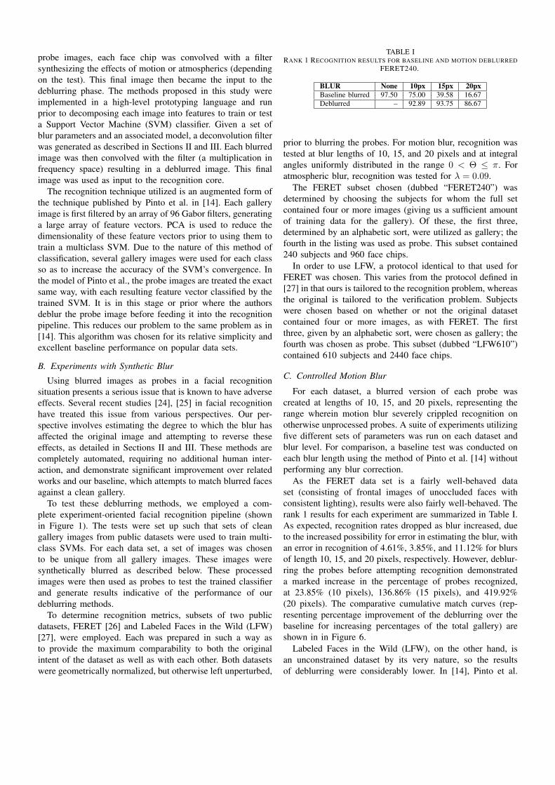
TABLE IRANK 1 RECOGNITION RESULTS FOR BASELINE AND MOTION DEBLURRED

FERET240.

BLUR None 10px 15px 20pxBaseline blurred 97.50 75.00 39.58 16.67Deblurred – 92.89 93.75 86.67

prior to blurring the probes. For motion blur, recognition wastested at blur lengths of 10, 15, and 20 pixels and at integralangles uniformly distributed in the range 0 < ⇥ ⇡. Foratmospheric blur, recognition was tested for � = 0.09.

The FERET subset chosen (dubbed “FERET240”) wasdetermined by choosing the subjects for whom the full setcontained four or more images (giving us a sufficient amountof training data for the gallery). Of these, the first three,determined by an alphabetic sort, were utilized as gallery; thefourth in the listing was used as probe. This subset contained240 subjects and 960 face chips.

In order to use LFW, a protocol identical to that used forFERET was chosen. This varies from the protocol defined in[27] in that ours is tailored to the recognition problem, whereasthe original is tailored to the verification problem. Subjectswere chosen based on whether or not the original datasetcontained four or more images, as with FERET. The firstthree, given by an alphabetic sort, were chosen as gallery; thefourth was chosen as probe. This subset (dubbed “LFW610”)contained 610 subjects and 2440 face chips.

C. Controlled Motion Blur

For each dataset, a blurred version of each probe wascreated at lengths of 10, 15, and 20 pixels, representing therange wherein motion blur severely crippled recognition onotherwise unprocessed probes. A suite of experiments utilizingfive different sets of parameters was run on each dataset andblur level. For comparison, a baseline test was conducted oneach blur length using the method of Pinto et al. [14] withoutperforming any blur correction.

As the FERET data set is a fairly well-behaved dataset (consisting of frontal images of unoccluded faces withconsistent lighting), results were also fairly well-behaved. Therank 1 results for each experiment are summarized in Table I.As expected, recognition rates dropped as blur increased, dueto the increased possibility for error in estimating the blur, withan error in recognition of 4.61%, 3.85%, and 11.12% for blursof length 10, 15, and 20 pixels, respectively. However, deblur-ring the probes before attempting recognition demonstrateda marked increase in the percentage of probes recognized,at 23.85% (10 pixels), 136.86% (15 pixels), and 419.92%(20 pixels). The comparative cumulative match curves (rep-resenting percentage improvement of the deblurring over thebaseline for increasing percentages of the total gallery) areshown in in Figure 6.

Labeled Faces in the Wild (LFW), on the other hand, isan unconstrained dataset by its very nature, so the resultsof deblurring were considerably lower. In [14], Pinto et al.

0

50

100

150

200

250

300

350

400

450

0.4 0.8 1.2 1.7 2.1 2.5 2.9 3.3 3.8 4.2

Perc

ent I

mpr

ovem

ent

Percent of Gallery

10 pixels15 pixels20 pixels

Fig. 6. Comparative cumulative match curves showing percent improvementfor our deblurring applied to images from the FERET240 set at three differentlevels of blur. Note the increasing improvement as the blur levels increase.

TABLE IIRANK 1 RECOGNITION RESULTS FOR BASELINE AND MOTION DEBLURRED

LFW610.

BLUR None 10px 15px 20pxBaseline blurred 41.64 19.34 10.33 5.08Deblurred – 33.11 24.26 16.89

treat the set from the perspective of a 1-to-1 face verificationproblem, using a protocol similar to that laid out in [27]. Thisprotocol is designed to test the problem of whether or not twofaces presented are of the same person. Using this technique,they demonstrate a 79.35% rate of success. This result is quitegood, considering that chance for the verification protocol is50%.

However, this paper approaches the dataset from the per-spective of a recognition problem, testing the problem of

20

40

60

80

100

120

140

160

180

200

220

240

0.2 0.3 0.5 0.7 0.8 1.0 1.1 1.3 1.5 1.6

Perc

ent I

mpr

ovem

ent

Percent of Gallery

10 pixels15 pixels20 pixels

Fig. 7. Comparative cumulative match curves showing percent improvementfor our deblurring applied to images from the LFW610 set at three differentlevels of blur. Note the increasing improvement as the blur levels increase.

TABLE IIIRANK 1 RECOGNITION RESULTS ON ATMOSPHERIC DEBLURRED SETS.

� = 0.09 IN EQUATION 8, REPRESENTING MODERATELY SEVERE BLUR.

No Blur Blurred DeblurredFERET240 97.50 37.08 90.68LFW610 41.64 9.34 37.54

classifying a picture as having been taken of a particularsubject (out of a gallery of several). Thus, the problem isconsiderably harder; chance for recognition is 1 in N , whereN is the number of subjects in the gallery. As LFW isconsidered to be one of the hardest set of faces for recognition,it is expected that recognition rates will be considerablylower than those obtained on other, more constrained, datasets.Thus, the numbers presented may appear low compared tothe FERET240 results (fulfilling expectations), but are, infact, demonstrative of a marked performance increase due todeblurring.

Table II summarizes the results obtained from attemptinga recognition-style experimental protocol on LFW610. Asdescribed above, recognition on a clean copy of the datasetis 41.64%, which is quite a bit lower than the 97.50%obtained on FERET240. However, as the effect of blur furtherreduces this rank 1 recognition rate, it can easily be seen thatdeblurring provides a considerable increase in recognition ratesat 71.2% for a blur of 10 pixels, 134.85% at 15 pixels, and232.48% at 20 pixels. Due to the difficulty of the dataset,it is not surprising that the recognition error due to blur andsubsequent estimation error is 20.49% (10 pixels), 41.74% (20pixels), and 59.44% (20 pixels), which is considerably greaterthan the respective numbers for FERET240. The comparativecumulative match curves are shown in Figure 7.

D. Controlled Atmospheric Blur

For each dataset, the atmospheric blur correction techniquewas tested with moderately severe synthetic atmospheric blur(� = 0.09 in Equation 8). Two sets of tests were performed:one on synthetically blurred probes to establish a baseline andone on deblurred versions of these probes. The rank 1 resultsare summarized, along with the results of recognition on cleanprobes, in Table III.

On FERET240, the atmospheric deblurring technique pre-sented demonstrated a relatively minimal recognition error dueto blur at a mere 7%, while exhibiting a drastic 144.55%increase in recognition rate over that of the blurred probes.The results for LFW610 were also very strong with a 301.93%increase in recognition rate over the blurred probes, while onlysuffering a 10.92% error due to the blur. Figure 8 presentscomparative cumulative match curves for the atmospheric blurexperiments for each of the two datasets.

E. Experiments with Real Blur

In order to further validate our approach, we processedseveral videos of subjects in motion in an outdoor settingat 100M. In total, three different videos were processed,

0

50

100

150

200

250

300

350

0.4/0.2 0.8/0.3 1.2/0.5 1.7/0.7 2.1/0.8 2.5/1.0 2.9/1.1 3.3/1.3 3.8/1.5 4.2/1.6

Perc

ent I

mpr

ovem

ent

Percent of Gallery (FERET240 / LFW610)

FERET240LFW610

Fig. 8. Comparative cumulative match curves showing percent improvementfor atmospheric blur experiments.

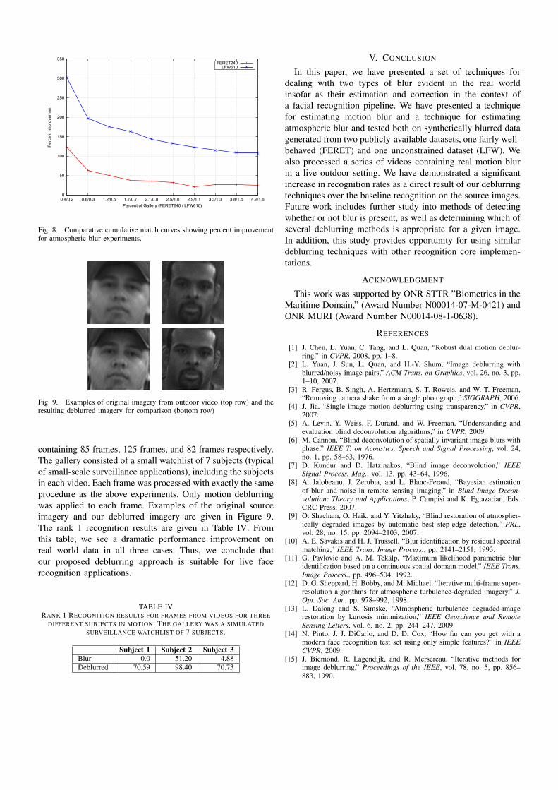
Fig. 9. Examples of original imagery from outdoor video (top row) and theresulting deblurred imagery for comparison (bottom row)

containing 85 frames, 125 frames, and 82 frames respectively.The gallery consisted of a small watchlist of 7 subjects (typicalof small-scale surveillance applications), including the subjectsin each video. Each frame was processed with exactly the sameprocedure as the above experiments. Only motion deblurringwas applied to each frame. Examples of the original sourceimagery and our deblurred imagery are given in Figure 9.The rank 1 recognition results are given in Table IV. Fromthis table, we see a dramatic performance improvement onreal world data in all three cases. Thus, we conclude thatour proposed deblurring approach is suitable for live facerecognition applications.

TABLE IVRANK 1 RECOGNITION RESULTS FOR FRAMES FROM VIDEOS FOR THREE

DIFFERENT SUBJECTS IN MOTION. THE GALLERY WAS A SIMULATEDSURVEILLANCE WATCHLIST OF 7 SUBJECTS.

Subject 1 Subject 2 Subject 3Blur 0.0 51.20 4.88Deblurred 70.59 98.40 70.73

V. CONCLUSION

In this paper, we have presented a set of techniques fordealing with two types of blur evident in the real worldinsofar as their estimation and correction in the context ofa facial recognition pipeline. We have presented a techniquefor estimating motion blur and a technique for estimatingatmospheric blur and tested both on synthetically blurred datagenerated from two publicly-available datasets, one fairly well-behaved (FERET) and one unconstrained dataset (LFW). Wealso processed a series of videos containing real motion blurin a live outdoor setting. We have demonstrated a significantincrease in recognition rates as a direct result of our deblurringtechniques over the baseline recognition on the source images.Future work includes further study into methods of detectingwhether or not blur is present, as well as determining which ofseveral deblurring methods is appropriate for a given image.In addition, this study provides opportunity for using similardeblurring techniques with other recognition core implemen-tations.

ACKNOWLEDGMENT

This work was supported by ONR STTR ”Biometrics in theMaritime Domain,” (Award Number N00014-07-M-0421) andONR MURI (Award Number N00014-08-1-0638).

REFERENCES

[1] J. Chen, L. Yuan, C. Tang, and L. Quan, “Robust dual motion deblur-ring,” in CVPR, 2008, pp. 1–8.

[2] L. Yuan, J. Sun, L. Quan, and H.-Y. Shum, “Image deblurring withblurred/noisy image pairs,” ACM Trans. on Graphics, vol. 26, no. 3, pp.1–10, 2007.

[3] R. Fergus, B. Singh, A. Hertzmann, S. T. Roweis, and W. T. Freeman,“Removing camera shake from a single photograph,” SIGGRAPH, 2006.

[4] J. Jia, “Single image motion deblurring using transparency,” in CVPR,2007.

[5] A. Levin, Y. Weiss, F. Durand, and W. Freeman, “Understanding andevaluation blind deconvolution algorithms,” in CVPR, 2009.

[6] M. Cannon, “Blind deconvolution of spatially invariant image blurs withphase,” IEEE T. on Acoustics, Speech and Signal Processing, vol. 24,no. 1, pp. 58–63, 1976.

[7] D. Kundur and D. Hatzinakos, “Blind image deconvolution,” IEEESignal Process. Mag., vol. 13, pp. 43–64, 1996.

[8] A. Jalobeanu, J. Zerubia, and L. Blanc-Feraud, “Bayesian estimationof blur and noise in remote sensing imaging,” in Blind Image Decon-volution: Theory and Applications, P. Campisi and K. Egiazarian, Eds.CRC Press, 2007.

[9] O. Shacham, O. Haik, and Y. Yitzhaky, “Blind restoration of atmospher-ically degraded images by automatic best step-edge detection,” PRL,vol. 28, no. 15, pp. 2094–2103, 2007.

[10] A. E. Savakis and H. J. Trussell, “Blur identification by residual spectralmatching,” IEEE Trans. Image Process., pp. 2141–2151, 1993.

[11] G. Pavlovic and A. M. Tekalp, “Maximum likelihood parametric bluridentification based on a continuous spatial domain model,” IEEE Trans.Image Process., pp. 496–504, 1992.

[12] D. G. Sheppard, H. Bobby, and M. Michael, “Iterative multi-frame super-resolution algorithms for atmospheric turbulence-degraded imagery,” J.Opt. Soc. Am., pp. 978–992, 1998.

[13] L. Dalong and S. Simske, “Atmospheric turbulence degraded-imagerestoration by kurtosis minimization,” IEEE Geoscience and RemoteSensing Letters, vol. 6, no. 2, pp. 244–247, 2009.

[14] N. Pinto, J. J. DiCarlo, and D. D. Cox, “How far can you get with amodern face recognition test set using only simple features?” in IEEECVPR, 2009.

[15] J. Biemond, R. Lagendijk, and R. Mersereau, “Iterative methods forimage deblurring,” Proceedings of the IEEE, vol. 78, no. 5, pp. 856–883, 1990.

[16] W. Fawwaz A M, T. Shimahashi, M. Matsubara, and S. Sugimoto, “PSFestimation and image restoration for noiseless motion blurred images,”in SSIP, 2008, pp. 1–7.

[17] R. Lokhande, K. Arya, and P. Gupta, “Identification of parametersand restoration of motion blurred images,” in ACM. Symp. on AppliedComputing, 2006, pp. 301–315.

[18] S. Wu, Z. Lu, E. Ong, and W. Lin, “Blind image blur identification incepstrum domain,” in ICCCN, 2007, pp. 1166–1171.

[19] K. Rajeswari, K. Krishna, V. Naveen, and A. Vamsidhar, “Performancecomparison of wiener filter and cls filter on 2d signals,” in ITNG, 2009,pp. 1244–1249.

[20] J. Thong, K. Sim, and J. Phang, “Single-image signal to noise ratioestimation,” Scanning, vol. 23, pp. 328–336, 2001.

[21] T. Boult and W. Scheirer, “Long range facial image acquisition andquality,” in Handbook of Remote Biometrics, M. Tistarelli, S. Li, andR. Chellappa, Eds. Springer, 2009.

[22] P. Qiu, “A nonparametric procedure for blind image deblurring,” Com-putational Statistics and Data Analysis, vol. 52, pp. 4828–4841, 2008.

[23] D. Bolme, R. Beveridge, M. Teixeira, and B. Draper, “The CSU FaceIdentification Evaluation System: Its purpose, features and structure,” inICVS, 2003, pp. 304–311.

[24] Q. Han, M. Zhang, C. Song, Z. Wang, and X. Niu, “A face imagedatabase for evaluating out-of-focus blur,” in ISDA, vol. 2, 2008, pp.277–282.

[25] M. Nishiyama, H. Takeshima, J. Shotton, T. Kozakaya, and O. Yam-aguchi, “Facial deblur inference to improve recognition of blurred faces,”in CVPR, 2009, pp. 1115–1122.

[26] P. J. Phillips, H. Moon, P. J. Rauss, and S. Rizvi, “The FERET evaluationmethodology for face recognition algorithms,” IEEE TPAMI, vol. 22,no. 10, 2000.

[27] G. Huang, M. Ramesh, T. Berg, and E. Learned-Miller, “Labeled facesin the wild: A database for studying face recognition in unconstrainedenvironments,” University of Massachusetts, Amherst, Tech. Rep. 07-49,2007.