
Towards non-conventional face recognition
169
THESE pour obtenir le grade de DOCTEUR DE L’ECOLE CENTRALE DE LYON Spécialité: Informatique Towards Non-Conventional Face Recognition: Shadow Removal and Heterogeneous Scenario dans le cadre de l’Ecole Doctorale InfoMaths présentée et soutenue publiquement par Wuming Zhang 17 Juillet 2017 Directeur de thèse: Prof. Jean-Marie MORVAN Co-directeur de thèse: Prof. Liming CHEN JURY Prof. Stan Z. Li Institute of Automation Rapporteur (Chinese Academy of Sciences) Prof. Stefano Berretti University of Florence Rapporteur DR1. Isabelle E. Magnin Créatis & Recherche Inserm Examinateur Dr. Séverine Dubuisson ISIR (UPMC) Examinateur Dr. Stéphane Gentric Morpho (Safran) Examinateur Prof. Jean-Marie Morvan Université Lyon 1 & KAUST Directeur de thèse Prof. Liming CHEN Ecole Centrale de Lyon Co-directeur de thèse
-
Upload
khangminh22 -
Category
Documents
-
view
1 -
download
0
Transcript of Towards non-conventional face recognition

THESE
pour obtenir le grade de
DOCTEUR DE L’ECOLE CENTRALE DE LYON
Spécialité: Informatique
Towards Non-Conventional Face Recognition:Shadow Removal and Heterogeneous Scenario
dans le cadre de l’Ecole Doctorale InfoMaths
présentée et soutenue publiquement par
Wuming Zhang
17 Juillet 2017
Directeur de thèse: Prof. Jean-Marie MORVAN
Co-directeur de thèse: Prof. Liming CHEN
JURY
Prof. Stan Z. Li Institute of Automation Rapporteur(Chinese Academy of Sciences)
Prof. Stefano Berretti University of Florence RapporteurDR1. Isabelle E. Magnin Créatis & Recherche Inserm ExaminateurDr. Séverine Dubuisson ISIR (UPMC) ExaminateurDr. Stéphane Gentric Morpho (Safran) ExaminateurProf. Jean-Marie Morvan Université Lyon 1 & KAUST Directeur de thèseProf. Liming CHEN Ecole Centrale de Lyon Co-directeur de thèse

2

For Li,
the love of my life.


Acknowledments
First and foremost, I would like to express my sincere and deep gratitude to my
advisors, Prof. Jean-Marie Morvan and Prof. Liming Chen. From affording me an
opportunity to work in their research team in 2011, to reviewing and proofreading
my thesis recently in 2017, they have been a constant source of wisdom and cre-
ativity. Working with these knowledgeable, enthusiastic and open-minded persons
has truly strengthened my passion for science.
I would like to thank the members of my PhD thesis committee: Prof. Stan Z.
Li, Prof. Stefano Berretti, DR1. Isabelle E. Magnin, Dr. Séverine Dubuisson and
Dr. Stéphane Gentric for accepting to evaluate this work and for their meticulous
evaluations and valuable comments.
A special thanks to Prof. Dimitris Samaras and Prof. Yunhong Wang for
their guidance and insightful remarks with respect to my paper organization and
submission. I would also like to express my thanks to my co-authors Dr. Di Huang,
Dr. Xi Zhao for their collaboration, thoughtful advise and significant help on the
writing and proofreading of our papers.
In addition, I am also grateful to all the colleagues and friends in Lyon (too many
to list all of them), including: Dr. Huanzhang Fu, Dr. Chao Zhu, Dr. Boyang Gao,
Dr. Huibin Li, Dr. Yuxing Tang, Dr. Yang Xu, Dr. Dongming Chen, Dr. Huiliang
Jin, Dr. Xiaofang Wang, Dr. Huaxiong Ding, Dr. Ying Lu, Dr. Chen Wang, Dr.
Yinhang Tang, Dr. Md Abul Hasnat, Wei Chen, Fei Zheng, Zehua Fu, Qinjie Ju,
Haoyu Li, Xiangnan Yin and Richard Marriott. The six-year life in Lyon will not
be so colorful and memorable without all happy times I’ve spent with you.
Last but most importantly, great thanks to my parents and all my family mem-
bers for their constant care and encouragement. Specifically, I would like to dedicate
this thesis to Li, my girlfriend, for being there with me through every step on our
journey from Beijing to Lyon, from Phuket to St. Petersburg, and from Lofoten to

0. Acknowledments
Canary Islands. As an answer to all my questions, a remedy to all my ailments and
a solution to all my problems, she is the best thing that ever happened to me.
iv

Abstract
In recent years, biometrics have received substantial attention due to the ever-
growing need for automatic individual authentication. Among various physiolog-
ical biometric traits, face offers unmatched advantages over the others, such as
fingerprints and iris, because it is natural, non-intrusive and easily understand-
able by humans. Nowadays conventional face recognition techniques have attained
quasi-perfect performance in a highly constrained environment wherein poses, illu-
minations, expressions and other sources of variations are strictly controlled. How-
ever these approaches are always confined to restricted application fields because
non-ideal imaging environments are frequently encountered in practical cases. To
adaptively address these challenges, this dissertation focuses on this unconstrained
face recognition problem, where face images exhibit more variability in illumination.
Moreover, another major question is how to leverage limited 3D shape information
to jointly work with 2D based techniques in a heterogeneous face recognition system.
To deal with the problem of varying illuminations, we explicitly build the un-
derlying reflectance model which characterizes interactions between skin surface,
lighting source and camera sensor, and elaborate the formation of face color. With
this physics-based image formation model involved, an illumination-robust repre-
sentation, namely Chromaticity Invariant Image (CII), is proposed which can sub-
sequently help reconstruct shadow-free and photo-realistic color face images. Due
to the fact that this shadow removal process is achieved in color space, this ap-
proach could thus be combined with existing gray-scale level lighting normalization
techniques to further improve face recognition performance. The experimental re-
sults on two benchmark databases, CMU-PIE and FRGC Ver2.0, demonstrate the
generalization ability and robustness of our approach to lighting variations.
We further explore the effective and creative use of 3D data in heterogeneous
face recognition. In such a scenario, 3D face is merely available in the gallery set

0. Abstract
and not in the probe set, which one would encounter in real-world applications.
Two Convolutional Neural Networks (CNN) are constructed for this purpose.
The first CNN is trained to extract discriminative features of 2D/3D face im-
ages for direct heterogeneous comparison, while the second CNN combines an
encoder-decoder structure, namely U-Net, and Conditional Generative Adversarial
Network (CGAN) to reconstruct depth face image from its counterpart in 2D.
Specifically, the recovered depth face images can be fed to the first CNN as well for
3D face recognition, leading to a fusion scheme which achieves gains in recognition
performance. We have evaluated our approach extensively on the challenging
FRGC 2D/3D benchmark database. The proposed method compares favorably to
the state-of-the-art and show significant improvement with the fusion scheme.
Keywords: face recognition, shadow removal, lighting normalization, deep
learning, convolutional neural networks, depth recovery
vi

Résumé
Ces dernières années, la biométrie a fait l’objet d’une grande attention en rai-
son du besoin sans cesse croissant d’authentification d’identité, notamment pour
sécuriser de plus en plus d’applications enlignes. Parmi divers traits biométriques,
le visage offre des avantages compétitifs sur les autres, e.g., les empreintes digitales
ou l’iris, car il est naturel, non-intrusif et facilement acceptable par les humains.
Aujourd’hui, les techniques conventionnelles de reconnaissance faciale ont atteint
une performance quasi-parfaite dans un environnement fortement contraint où la
pose, l’éclairage, l’expression faciale et d’autres sources de variation sont sévère-
ment contrôlées. Cependant, ces approches sont souvent confinées aux domaines
d’application limités parce que les environnements d’imagerie non-idéaux sont très
fréquents dans les cas pratiques. Pour relever ces défis d’une manière adaptative,
cette thèse porte sur le problème de reconnaissance faciale non contrôlée, dans lequel
les images faciales présentent plus de variabilités sur les éclairages. Par ailleurs, une
autre question essentielle vise à profiter des informations limitées de 3D pour colla-
borer avec les techniques basées sur 2D dans un système de reconnaissance faciale
hétérogène.
Pour traiter les diverses conditions d’éclairage, nous construisons explicitement
un modèle de réflectance en caractérisant l’interaction entre la surface de la peau,
les sources d’éclairage et le capteur de la caméra pour élaborer une explication de la
couleur du visage. A partir de ce modèle basé sur la physique, une représentation
robuste aux variations d’éclairage, à savoir Chromaticity Invariant Image (CII),
est proposée pour la reconstruction des images faciales couleurs réalistes et sans
ombre. De plus, ce processus de la suppression de l’ombre en niveaux de couleur
peut être combiné avec les techniques existantes sur la normalisation d’éclairage en
niveaux de gris pour améliorer davantage la performance de reconnaissance faciale.
Les résultats expérimentaux sur les bases de données de test standard, CMU-PIE

0. Résumé
et FRGC Ver2.0, démontrent la capacité de généralisation et la robustesse de notre
approche contre les variations d’éclairage.
En outre, nous étudions l’usage efficace et créatif des données 3D pour la
reconnaissance faciale hétérogène. Dans un tel scénario asymétrique, un enrôle-
ment combiné est réalisé en 2D et 3D alors que les images de requête pour la
reconnaissance sont toujours les images faciales en 2D. A cette fin, deux Réseaux
de Neurones Convolutifs (Convolutional Neural Networks, CNN) sont construits.
Le premier CNN est formé pour extraire les descripteurs discriminants d’images
2D/3D pour un appariement hétérogène. Le deuxième CNN combine une structure
codeur-décodeur, à savoir U-Net, et Conditional Generative Adversarial Network
(CGAN), pour reconstruire l’image faciale en profondeur à partir de son homologue
dans l’espace 2D. Plus particulièrement, les images reconstruites en profondeur
peuvent être également transmise au premier CNN pour la reconnaissance faciale
en 3D, apportant un schéma de fusion qui est bénéfique pour la performance en
reconnaissance. Notre approche a été évaluée sur la base de données 2D/3D de
FRGC. Les expérimentations ont démontré que notre approche permet d’obtenir
des résultats comparables à ceux de l’état de l’art et qu’une amélioration significa-
tive a pu être obtenue à l’aide du schéma de fusion.
Mots-clés: reconnaissance faciale, suppression des ombres, normalisation
d’éclairage, apprentissage profond, réseaux de neurones convolutionnels, recon-
struction de profondeur
viii

Contents
Acknowledments iii
Abstract v
Résumé vii
1 Introduction 1
1.1 Background . . . . . . . . . . . . . . . . . . . . . . . . . . . . . . . . 2
1.1.1 Biometrics: Changes in the Authentication Landscape . . . . 2
1.1.2 Face: Leading Candidate in Biometrics . . . . . . . . . . . . 5
1.2 2D & 3D Face Recognition: Successes and Challenges . . . . . . . . 7
1.2.1 2D Face Recognition: Overview . . . . . . . . . . . . . . . . . 8
1.2.2 Challenges for 2D Face Recognition . . . . . . . . . . . . . . 12
1.2.3 3D: Opportunity or Challenge? . . . . . . . . . . . . . . . . . 16
1.2.4 2D/3D Heterogeneous Face Recognition . . . . . . . . . . . . 19
1.3 Approaches and Contributions . . . . . . . . . . . . . . . . . . . . . 19
1.3.1 Improving Shadow Suppression for Illumination Invariant
Face Recognition . . . . . . . . . . . . . . . . . . . . . . . . . 20
1.3.2 Heterogeneous Face Recognition with Convolutional Neural
Networks . . . . . . . . . . . . . . . . . . . . . . . . . . . . . 20
1.4 Outline . . . . . . . . . . . . . . . . . . . . . . . . . . . . . . . . . . 21
2 Literature Review 23
2.1 2D Face Recognition Techniques . . . . . . . . . . . . . . . . . . . . 24
2.1.1 Holistic feature based methods . . . . . . . . . . . . . . . . . 24
2.1.2 Local feature based methods . . . . . . . . . . . . . . . . . . 25
2.1.3 Hybrid methods . . . . . . . . . . . . . . . . . . . . . . . . . 27
2.1.4 Deep learning based methods . . . . . . . . . . . . . . . . . . 27
2.2 Illumination Insensitive Approaches . . . . . . . . . . . . . . . . . . 30

Contents
2.2.1 Image Enhancement based Approaches . . . . . . . . . . . . . 30
2.2.2 Illumination Insensitive Feature based Approaches . . . . . . 31
2.2.3 Illumination Modeling based Approaches . . . . . . . . . . . 36
2.2.4 3D Model based Approaches . . . . . . . . . . . . . . . . . . 38
2.3 2D/3D Heterogeneous Face Recognition . . . . . . . . . . . . . . . . 40
2.3.1 Common subspace learning . . . . . . . . . . . . . . . . . . . 40
2.3.2 Synthesis Methods . . . . . . . . . . . . . . . . . . . . . . . . 44
2.4 Conclusion . . . . . . . . . . . . . . . . . . . . . . . . . . . . . . . . 47
3 Improving Shadow Suppression for Illumination Robust Face
Recognition 49
3.1 Introduction . . . . . . . . . . . . . . . . . . . . . . . . . . . . . . . . 50
3.2 Skin Color Analysis . . . . . . . . . . . . . . . . . . . . . . . . . . . 53
3.2.1 Reflectance Model: Lambert vs. Phong . . . . . . . . . . . . 53
3.2.2 Specular Highlight Detection . . . . . . . . . . . . . . . . . . 54
3.2.3 Skin Color Formation . . . . . . . . . . . . . . . . . . . . . . 56
3.3 Chromaticity Invariant Image . . . . . . . . . . . . . . . . . . . . . . 58
3.3.1 Skin Model in Chromaticity Space . . . . . . . . . . . . . . . 58
3.3.2 Chromaticity Invariant Image Generation . . . . . . . . . . . 59
3.3.3 Entropy based Lighting Normalization . . . . . . . . . . . . . 62
3.3.4 Global Intensity Regularization . . . . . . . . . . . . . . . . . 64
3.4 Shadow-free Color Face Recovery . . . . . . . . . . . . . . . . . . . . 64
3.4.1 In-depth Analysis of 1D Chromaticity Image . . . . . . . . . 64
3.4.2 Shadow-Specific Edge Detection . . . . . . . . . . . . . . . . 66
3.4.3 Full Color Face Image Reconstruction . . . . . . . . . . . . . 67
3.5 Experimental Results . . . . . . . . . . . . . . . . . . . . . . . . . . . 69
3.5.1 Databases and Experimental Settings . . . . . . . . . . . . . 69
3.5.2 Visual Comparison and Discussion . . . . . . . . . . . . . . . 73
3.5.3 Identification Results on CMU-PIE . . . . . . . . . . . . . . . 77
3.5.4 Verification Results on FRGC . . . . . . . . . . . . . . . . . . 80
3.6 Conclusion . . . . . . . . . . . . . . . . . . . . . . . . . . . . . . . . 83
x

Contents
4 Improving 2D-2.5D Heterogeneous Face Recognition with Condi-
tional Adversarial Networks 85
4.1 Introduction . . . . . . . . . . . . . . . . . . . . . . . . . . . . . . . . 86
4.2 Baseline Cross-encoder Model . . . . . . . . . . . . . . . . . . . . . . 88
4.2.1 Background on Autoencoder . . . . . . . . . . . . . . . . . . 89
4.2.2 Discriminative Cross-Encoder . . . . . . . . . . . . . . . . . . 91
4.2.3 Multi-Criterion Mechanism . . . . . . . . . . . . . . . . . . . 94
4.2.4 Heterogeneous Face Recognition . . . . . . . . . . . . . . . . 96
4.3 CGAN based HFR Framework . . . . . . . . . . . . . . . . . . . . . 96
4.3.1 Background on CGAN . . . . . . . . . . . . . . . . . . . . . . 97
4.3.2 CGAN Architecture . . . . . . . . . . . . . . . . . . . . . . . 99
4.3.3 Heterogeneous Face Recognition . . . . . . . . . . . . . . . . 101
4.4 Experimental Results . . . . . . . . . . . . . . . . . . . . . . . . . . . 104
4.4.1 Dataset Collection . . . . . . . . . . . . . . . . . . . . . . . . 104
4.4.2 Implementation details . . . . . . . . . . . . . . . . . . . . . . 107
4.4.3 Reconstruction Results . . . . . . . . . . . . . . . . . . . . . . 108
4.4.4 2D-3D Asymmetric FR . . . . . . . . . . . . . . . . . . . . . 110
4.5 Conclusion . . . . . . . . . . . . . . . . . . . . . . . . . . . . . . . . 113
5 Conclusion and Future Work 115
5.1 Contributions . . . . . . . . . . . . . . . . . . . . . . . . . . . . . . . 116
5.1.1 Improving Shadow Suppression for Illumination Robust Face
Recognition . . . . . . . . . . . . . . . . . . . . . . . . . . . . 116
5.1.2 Improving Heterogeneous Face Recognition with Conditional
Adversarial Networks . . . . . . . . . . . . . . . . . . . . . . 117
5.2 Perspective for Future Directions . . . . . . . . . . . . . . . . . . . . 117
5.2.1 Pose Invariant Heterogeneous Face Recognition . . . . . . . . 117
5.2.2 Transfer to Other Heterogeneous Face Recognition Scenarios 118
5.2.3 Integration of Unconstrained Face Recognition Techniques . . 118
6 List of Publications 119
xi

Contents
Bibliography 121
xii

List of Tables
1.1 A brief comparison of biometric traits . . . . . . . . . . . . . . . . . 5
1.2 List of commonly used constrained 2D face databases. E: expression.
I: illumination. O: occlusion. P: pose. T: time sequences. . . . . . . 9
1.3 List of large-scale unconstrained 2D face databases . . . . . . . . . . 9
1.4 The confusion matrix created by the prediction result of the face
recognition system (S) and ground truth condition. I: provided au-
thentication proof. C: claimed identity. T: true. F: false. P: posi-
tive. N: negative. R: rate. . . . . . . . . . . . . . . . . . . . . . . . . 11
1.5 List of commonly used 3D face databases . . . . . . . . . . . . . . . 17
3.1 Overview of database division in our experiments . . . . . . . . . . . 71
3.2 Rank-1 Recognition Rates (Percent) of Different Methods on CMU-
PIE Database . . . . . . . . . . . . . . . . . . . . . . . . . . . . . . . 79
3.3 Verification Rate (Percent) at FAR = 0.1% Using Different Methods
on FRGC V2.0 Exp.4 . . . . . . . . . . . . . . . . . . . . . . . . . . 81
4.1 Database overview. E and I are short for expressions and illumina-
tions, respectively. . . . . . . . . . . . . . . . . . . . . . . . . . . . . 105
4.2 Comparison of recognition accuracy on FRGC under different pro-
tocols. Note that some blank numbers are reported in this table
because we strictly follow the protocol defined in each related lit-
erature, e.g. the gallery set in [Wang et al. 2014] solely contains
depth images, when compared with their work, our experiment will
subsequently exclude 2D based matching to respect this protocol. . . 112
4.3 2D/2.5D HFR accuracy of cGAN-CE with varying λ under protocol
of [Huang et al. 2012]. . . . . . . . . . . . . . . . . . . . . . . . . . . 113


List of Figures
1.1 Examples of commonly used biometric traits . . . . . . . . . . . . . 4
1.2 Human face samples captured under different modalities. . . . . . . 6
1.3 General workflow of a face recognition system . . . . . . . . . . . . . 8
1.4 A person with the same pose and expression under different illumina-
tion conditions. Images are extracted from the CMU-PIE database
[Sim et al. 2003]. . . . . . . . . . . . . . . . . . . . . . . . . . . . . . 12
1.5 Photographs of David Beckham with varying head poses . . . . . . . 13
1.6 Photographs of Yunpeng Yue with varying facial expressions . . . . 14
1.7 Photographs of Queen Elizabeth II at different ages . . . . . . . . . 14
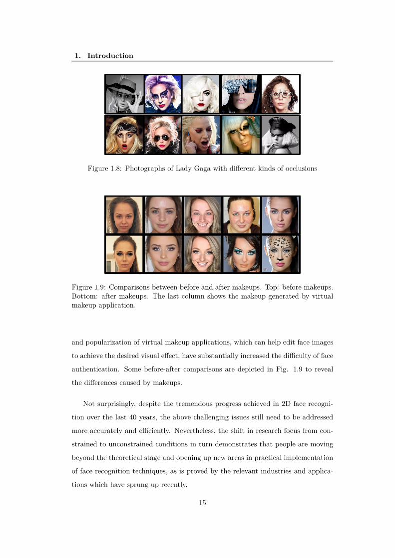
1.8 Photographs of Lady Gaga with different kinds of occlusions . . . . . 15
1.9 Comparisons between before and after makeups. Top: before make-
ups. Bottom: after makeups. The last column shows the makeup
generated by virtual makeup application. . . . . . . . . . . . . . . . 15
1.10 Examples of data corruption in captured 3D samples. Corruption
conditions include missing parts, spikes and noise observed in [Lei
et al. 2016] and [Bowyer et al. 2006]. . . . . . . . . . . . . . . . . . . 18
2.1 Eigenfaces scheme. . . . . . . . . . . . . . . . . . . . . . . . . . . . . 25
2.2 Schema of LBP operator. (a) An example of LBP encoding schema
with P = 8. (b) Examples of LBP patterns with different numbers
of sampling points and radius. [Huang et al. 2011] . . . . . . . . . . 26
2.3 The first convolutional neural network for face recognition [Lawrence
et al. 1997]. . . . . . . . . . . . . . . . . . . . . . . . . . . . . . . . . 29
2.4 Outline of the Deepface architecture proposed in [Taigman et al. 2014]. 29
2.5 Visual comparison for face images normalized with different illumi-
nation preprocessing methods on databases with controlled and less-
controlled lighting [Han et al. 2013]. . . . . . . . . . . . . . . . . . . 36
2.6 Patch based CCA for 2D-3D matching proposed in [Yang et al. 2008]. 41

List of Figures
2.7 The 2D-3D face recognition framework proposed in [Wang
et al. 2014]. (a): Illustration of training and testing scheme. (b):
Illustration of principal components of the scheme. . . . . . . . . . . 43
2.8 Intuitive explanation of the Multiview Smooth Discriminant Analysis
based Extreme Learning Machines (ELM) approach [Jin et al. 2014]. 44
2.9 Overview of the reference 3D-2D face recognition system with illu-
mination normalization between probe and gallery textures [Toderici
et al. 2010]. . . . . . . . . . . . . . . . . . . . . . . . . . . . . . . . . 45
3.1 An example of varying lighting conditions for the same face. (a)
Front lighting; (b) Specular highlight due to glaring light coming
from right side; (c) Soft shadows and (d) hard-edged cast shadow. . 51
3.2 Overview of the chromaticity space based lighting normalization pro-
cess and shadow-free color face recovery process. . . . . . . . . . . . 52
3.3 Specular highlight detection results on images under various lighting
conditions. First row and third row: original images; second row and
fourth row: detected highlight masks. . . . . . . . . . . . . . . . . . 56
3.4 Linearity of chromaticity image pixels in log space. (a) Original
image. (b) chromaticity pixel values in 3D log space. (c) Pixels of
forehead area in projected plane. (d) Pixels of nose bridge area in
projected plane. . . . . . . . . . . . . . . . . . . . . . . . . . . . . . . 61
3.5 Overview of chromaticity invariant image generation. Left column:
original face image and its chromaticity points in 2D log space; mid-
dle column: entropy diagram as a function of projection angle, the
arrows in red indicate projection directions at that point; right col-
umn: generated chromaticity images with different angle values. . . . 63
xvi

List of Figures
3.6 Overview of edge mask detection and full color face recovery. (a)
and (f) are raw and recovered face image; (b), (c) and (d) depict
respectively 1D/2D chromaticity images and edge maps, note that
in each figure the upper row refers to shadow-free version and the
lower row is shadow-retained version; (e) is the final detected edge
mask. . . . . . . . . . . . . . . . . . . . . . . . . . . . . . . . . . . . 69
3.7 Cropped face examples of the first subject in the (a): CMU-PIE
database; (b): FRGC database. . . . . . . . . . . . . . . . . . . . . . 71
3.8 Holistic and local shadow removal results on hard-edged shadows
(left) and soft shadows (right). . . . . . . . . . . . . . . . . . . . . . 74
3.9 Illustration of illumination normalization performance of two sam-
ples in (a) CMU-PIE and (b) FRGC database. For each sample,
three lighting conditions are considered, from top to bottom are the
image with frontal lighting, image with soft shadows and image with
hard-edged shadows.The columns represent different lighting nor-
malization techniques to be fused with original color image or CII
recovered color image. Green framed box: a comparison sample pair
with soft shadows. Red framed box: a comparison sample pair with
hard-edged shadows. . . . . . . . . . . . . . . . . . . . . . . . . . . . 75
3.10 Faces in the wild before (top) and after (bottom) shadow removal.
From left to right we choose images with a gradual decrease (left:
strong, middle two: moderate, right: weak) in shadow intensity. . . . 77
3.11 Several ROC curves for different gray-scale methods. (a) No gray-
scale method, (b) GRF, (c) DOG, (d) WEB, (e) SQI, (f) TT. Note
that only (a) contains ROC curves for VGG-Face model because it
requires RGB images as model input. . . . . . . . . . . . . . . . . . . 82
xvii

List of Figures
4.1 The proposed baseline model takes one single RGB face image as
input and serves two purposes: (i) extract discriminative feature
through well-trained encoder and (ii) reconstruct a 2.5D range image
after decoder. The dual output will be used in the final fusion phase
of face recognition. . . . . . . . . . . . . . . . . . . . . . . . . . . . . 89
4.2 Architecture and training process of the proposed cross-encoder
framework. A 3×98×98 2D image is fed into the system with its
corresponding 2.5D image as the target. The kernel sizes of C1 is
6×6, and its stride is 3. C3 and C5 own the same kernel size 3×3
and the same stride 1. All convolutional layers in red, i.e. C2, C4
and C6, keep the kernel size as 2×2 and stride as 2, in this way they
play the role of pooling layers in other networks. The output vec-
tor representation of each fully connected layer is 4096-dimension.
The structure of decoder is omitted here because it simply reverses
the structure of encoder. All convolultional layers are followed by a
PReLU layer and a batch normalization layer. . . . . . . . . . . . . 92
4.3 The difference of processing method between a conventional max-
pooling layer and a pooling-like convolutional layer with kernel size
2×2 and stride 2. . . . . . . . . . . . . . . . . . . . . . . . . . . . . . 92
4.4 The comparison of outputs with and without the checkerboard ar-
tifacts. The left two images which benefit from well-adapted con-
volutional kernel size and gradient loss presents a smoother surface
with invisible checkerboard effect compared with the right-hand side
images which results from a conventional CNN. . . . . . . . . . . . . 93
4.5 Overview of the proposed CNN models for heterogeneous face recog-
nition. Note that (1) depth recovery is conducted only for testing;
(2) the final joint recognition may or may not include color based
matching, depending on the specific experiment protocol. . . . . . . 97
4.6 The mechanism of cGAN. . . . . . . . . . . . . . . . . . . . . . . . . 99
xviii

List of Figures
4.7 The architectures of Generator and Discriminator in our cGAN
model. In Fig. 4.7a, the noise variable z presents itself under the
the form of dropout layers, while the black arrows portray the skip
connections between encoder layer and decoder layer that are on the
’same’ level. All convolution and deconvolution layers are with filter
size 4×4 and 1-padding, n and s represent the number of output
channels and stride value, respectively. (Best view in color) . . . . . 100
4.8 Training procedure of the cross-modal CNN model. Models in the
dashed box are pre-trained using 2D and 2.5D face images individu-
ally. . . . . . . . . . . . . . . . . . . . . . . . . . . . . . . . . . . . . 103
4.9 Some face examples of 2D texture and 3D depth image in the FRGC
Ver2.0 face database. Top: 2D texture samples. Center: 3D depth
images before preprocessing. Bottom: 3D depth images after filling
holes and face region cropping. Note that the texture images shown
above are correspondingly preprocessed following the same rule with
depth images. . . . . . . . . . . . . . . . . . . . . . . . . . . . . . . . 106
4.10 Qualitative reconstruction results of FRGC samples with varying il-
luminations and expressions. . . . . . . . . . . . . . . . . . . . . . . 108
4.11 Several wrongly reconstructed samples. . . . . . . . . . . . . . . . . . 110
xix

1
Introduction
Contents1.1 Background . . . . . . . . . . . . . . . . . . . . . . . . . . . . . . 2
1.1.1 Biometrics: Changes in the Authentication Landscape . . . . 2
1.1.2 Face: Leading Candidate in Biometrics . . . . . . . . . . . . 5
1.2 2D & 3D Face Recognition: Successes and Challenges . . . . 7
1.2.1 2D Face Recognition: Overview . . . . . . . . . . . . . . . . . 8
1.2.2 Challenges for 2D Face Recognition . . . . . . . . . . . . . . 12
1.2.3 3D: Opportunity or Challenge? . . . . . . . . . . . . . . . . . 16
1.2.4 2D/3D Heterogeneous Face Recognition . . . . . . . . . . . . 19
1.3 Approaches and Contributions . . . . . . . . . . . . . . . . . . 19
1.3.1 Improving Shadow Suppression for Illumination Invariant Face
Recognition . . . . . . . . . . . . . . . . . . . . . . . . . . . . 20
1.3.2 Heterogeneous Face Recognition with Convolutional Neural
Networks . . . . . . . . . . . . . . . . . . . . . . . . . . . . . 20
1.4 Outline . . . . . . . . . . . . . . . . . . . . . . . . . . . . . . . . 21
“...On the other hand, when processing complex natural images such
as faces, the situation is complicated still further. There is such a wide
variety in the input images that measurement of features must be adaptive
to each individual image and relative to other feature measurements. We
shall be dealing with photographs of one full face with no glasses or beard.
We assume that the face in a photo may have tilt, forward inclination, or
be backward bent to a certain degree, but is never turned to one side.”
– Takeo Kanade, Doctoral Dissertation, 1973

1. Introduction
Back in 1973, when T. Kanade described the challenges and constraints for face
recognition in his doctoral dissertation [Kanade 1973], which is also publicly known
as the first paper talking about face recognition, he might not have foreseen the per-
vasive growth and striking development of this technique after more than 40 years.
Questions then naturally arise: Why is face recognition playing an increasingly im-
portant role in person identification? How does it work conceptually? What are
the main challenges? In this chapter we answer these questions and give a detailed
demonstration of how my thesis work is motivated and organized. Unless otherwise
specified, all images in this chapter are taken from public domain websites.
1.1 Background
1.1.1 Biometrics: Changes in the Authentication Landscape
The problem of authentication - verifying that someone is who he/she claims to be -
has existed since the beginning of human history. Unless it is answered satisfactorily,
identification is incomplete and no authorization can or should take place.
Our ancestors living in a primitive society were far less concerned with this issue
because their ordinary life was limited to a small community where everybody knew
each other. Basically, this means that the most original factors used to authenti-
cate an individual are something the user is, i.e. some inherent physical traits or
characteristics: face, voice, etc.
Along with social changes and technological developments, human activities
have been largely enhanced and an explosive growth of authentication cases and
patterns have emerged. At this stage, the factors for authenticating someone have
gradually shifted to something the person knows. This could be a reusable pass-
word, a personal identification number (PID) or a fact likely to be known only to
this person, such as his favorite movie; or something the person has, which could be
a key, a magnetic-stripe card, a smart card or a specialized authentication device
(called a security token) that generates a one-time password or a specific response to
a challenge presented by the server. Due to their ease of use and low cost, a variety
of productions based on both factors are widely used nowadays as authentication
2

1. Introduction
measures. However, these mechanisms have apparent drawbacks: password authen-
tication is vulnerable to a password “cracker”, another nightmare, who uses brute
force attack while managing multiple passwords for different systems: keys, smart
cards or other security tokens provide a relatively easier and safer authentication
mode, but there is the risk of their being lost or faked.
To further cope with these drawbacks, a stronger and securer authentication pro-
cess is needed. Thanks to the widespread use of data acquisition devices (e.g. dig-
ital cameras, scanners, smartphones) and the never-ending progress in algorithms,
biometrics have made a public return with a totally new look.
Biometric authentication involves the use of biological statistics to compute
the probability of two people having identical biological characteristics. Compared
with other authentication factors as mentioned above, biometrics are advantageous
across a series of attributes, including but not limited to:
1. User-Friendly: Users will no longer need to memorize a long list of passwords
or carry a set of keys. All they need to do is to present their biometrics and
let the system handle the rest.
2. Understandability: Identifying people by intrinsic biometrics such as face and
voice is essentially a human instinctive habit, which makes biometric authen-
tication easy to understand and interpret.
3. Security: Unlike passwords and keys, biometric authentication has been
widely regarded as the hardest to forge or spoof.
4. Accuracy: Higher level identification accuracy can be maximally ensured by
integrating multi-modal biometrics.
As a constant necessity, biometrics are used to identify authorized people based
on specific physiological or behavioral features. Examples of behavioral characteris-
tics are gait, signature and voice. Physical characteristics include: DNA, ear, face,
fingerprint, hand geometry, iris and retina. Some popular biometrics are illustrated
in Fig. 1.1. These biometrics are selected based on seven main criteria as proposed
in [Jain et al. 2006]:
3

1. Introduction
Figure 1.1: Examples of commonly used biometric traits
1. Uniqueness: Most importantly, each biometric should be sufficiently unique
for distinguishing one person from another.
2. Universality: Each person, irrespective of any external factors, should possess
his/her own biometric trait during an authentication process.
3. Permanence: To preserve the robustness of selected biometrics, the trait
should be invariant with one individual over a long period.
4. Collectability: A proper method or device can be easily applied to measure or
capture the biometric trait quantitatively.
5. Acceptability: The aforesaid collection pattern or the measurement mode of
the trait can be widely accepted by the public.
6. Circumvention: The vulnerability level of the underlying biometric system
with the given trait is acceptable under fraudulent attacks.
7. Performance: Both the accuracy and processing speed of the system involving
the trait are sufficiently satisfactory for the authentication requests.
4

1. Introduction
Table 1.1: A brief comparison of biometric traits
Biometric Trait
Face
Han
dV
eins
Fin
gerp
rint
Iris
Voi
ce
DN
A
Pal
mpr
int
Ear
Gai
t
Ret
ina
Sign
atur
e
Uniqueness M H H H L H H M L H L
Universality H H M H M H M M M H L
Permanence M H H H L H H H L M L
Collectability H M M M M L M M H L H
Acceptability H M M L H L M H H L H
Circumvention H M M L H L M M M L H
Performance H M H H L H H M L H L
1.1.2 Face: Leading Candidate in Biometrics
Among all biometric traits used for person identification, face based analysis has
recently received a great deal of attention due to the enormous developments in
the field of image processing and machine learning. Over and beyond its scientific
interest, when compared with other biometrics such as fingerprint and iris, face
offers a number of unmatched advantages for a wide variety of potential applications
in commerce and law enforcement. To intuitively demonstrate the advantages and
disadvantages of face and other biometric traits, in Table 1.1 we list a comparison
based on seven parameters in [Jain et al. 2006]. In this table, high, medium and
low are denoted by H, M and L, respectively.
From this table we can infer that face is superior to other biometrics due to the
following reasons:
- Non-intrusive process. Instead of requiring users to place their hand or fingers
on a reader (a process not acceptable in some cultures as well as being a source
of disease transfer) or to precisely position their eye in front of a scanner, face
recognition systems unobtrusively take photos of people’s faces at a distance.
No intrusion or delay is needed, and in most cases the users are entirely
5

1. Introduction
Figure 1.2: Human face samples captured under different modalities.
unaware of the capture process. They do not feel their privacy has been
invaded or ”under surveillance”. Moreover, identifying a person based on
his/her face is one of the oldest and most basic types of human behavior,
which also makes it naturally accepted by the public.
- Ease of implementation. Unlike most biometric traits which necessitate pro-
fessional equipment during their implementation (e.g. digital reader and scan-
ner for fingerprints, palm prints, iris and retina), face data can be easily cap-
tured via digital cameras, cameras on PCs or even the widespread use of
smartphones.
- Various modalities. In contrast with other biometric traits which are nor-
mally unimodal (mostly color/grayscale images), face data can be captured
and stored under a variety of modalities. Different modalities are exploited
in different face recognition scenarios according to their own characteristics.
Color images are sufficient for normal recognition tasks, depth images and
3D scans are more robust against lighting variations, face sketches are widely
used in the investigation of serious crimes by police, just to name a few.
Specifically, the collaboration between 2D images and 3D models markedly
improves face recognition performance. Several commonly used modalities
are illustrated in Fig. 1.2.
- Performance boost. Up to the first decade of this century, identification per-
formance based on face was relatively poor when compared with performance
based on other strong traits such as iris and retina [Jain et al. 2004]. The
main reason lies in the restricted ability of distinguishing a person in an
6

1. Introduction
unconstrained environment as face representations can be more sensitive to
variations in lighting, pose, expression, etc. However, over the last few years,
the performance of unconstrained face recognition has progressed consider-
ably with the emergence of deep learning. For instance, the state-of-the-art
image-unrestricted verification results on the challenging Labeled Faces in the
Wild (LFW) benchmark [Huang et al. 2007b] have been largely improved from
84.45% [Cao et al. 2010] to 99.53% [Schroff et al. 2015] over a period of four
years.
Besides the above-mentioned merits and other advantages, for example there is
no association with crime as with fingerprints (few people would object to looking at
a camera) and many existing systems already store face images (such as police mug
shots), face recognition also shows no weak points in any aspects as demonstrated
in Table 1.1, making it stably and reasonably accepted as a leading candidate in all
biometric traits. Nowadays, face recognition technology is becoming an ever closer
part of people’s daily lives in the form of relevant applications, including but not
limited to access control, suspect tracking, video surveillance and human computer
interaction.
1.2 2D & 3D Face Recognition: Successes and Chal-
lenges
The face recognition pipeline involves not only comparing two face images, but also
includes a complicated system dealing with a series of questions: Which databases
are required? Do we need any pre-processing methods? What kind of metric
should be used for performance evaluation? In this section, we start by describing
the principal mechanism and main drawbacks of 2D face recognition, followed by
an extended discussion of 3D face recognition technology. This section ends with
an introduction of 2D/3D heterogeneous face recognition.
7

1. Introduction
Figure 1.3: General workflow of a face recognition system
1.2.1 2D Face Recognition: Overview
The term ”face recognition” encompasses five main procedures, namely data prepa-
ration, pre-processing, feature extraction, pattern classification and performance
evaluation in a logical sequential order. Other steps might be optionally involved
depending on system requirements and algorithm properties, such as the use of
training samples for model learning. Fig. 1.3 depicts the general pipeline of a stan-
dard face recognition process. In this section, we accordingly provide below a brief
review for each procedure to enable comprehensive understanding.
Data preparation. Beyond all questions, accurate and appropriate data col-
lection is apparently a cornerstone of all face recognition research. The history
of 2D face database construction passes through two stages: first, conventional
face databases merely contain images under constrained conditions, which are nor-
mally guaranteed by data acquisition in a specified environment during the same
period; then people attempt to gather as many face images as possible to address
the unconstrained face recognition problem. The emergence and progress of deep
learning-based methods greatly foster the transition between these two stages. To
provide an intuitive overview, in Table 1.2 and 1.3 we list the most popular con-
strained and unconstrained 2D benchmark face databases, respectively.
Pre-processing. Quality of image plays a crucial role in increasing face recog-
nition performance. A good quality image yields a better recognition rate than
noisy or badly aligned images. To overcome problems occurring due to bad qual-
8

1. Introduction
Table 1.2: List of commonly used constrained 2D face databases. E: expression. I:illumination. O: occlusion. P: pose. T: time sequences.
Face Database Year # of subjects # of images Variations
ORL 1992-1994 40 400 E,I,O
Feret 1993-1997 1,199 14,126 E,I,P,T
Yale 1997 15 165 E,I,O
JAFFE 1998 10 213 E
AR 1998 126 >4,000 E,I,O
Yale-B 2001 10 5,850 I,P
CMU-PIE 2000 68 >40,000 E,I,P
CAS-PEAL 2005 1,040 99,594 E,I,O,P
Multi-PIE 2008 337 >750,000 E,I,P
Table 1.3: List of large-scale unconstrained 2D face databasesFace Database Year # of subjects # of images
LFW 2007 5,749 13,233
PubFig 2009 200 58,797
Youtube Faces 2011 1,595 3,425 videos
FaceScrub 2014 530 106,863
CACD2000 2014 2,000 >160,000
CASIA-Webface 2014 10,575 494,414
IJB-A 2015 500 5,712 images + 2,085 videos
CelebA 2015 10,177 202,599
MS-Celeb-1M 2016 99,952 10,490,534
MegaFace 2016 672,057 4,753,520
9
1. Introduction
ity, a variety of pre-processings are optional before extracting features from the
image. Generally, these techniques can be categorized into two classes: 1) spatial
transformations. An intuitive way to preprocess images for easier comparison is to
make them alike. To achieve this goal, several traditional and straightforward pre-
processing methods are provided: face detection and cropping, face resizing, face
alignment, etc. 2) image normalization. These methods are usually employed to re-
duce the effect of noise or different global lighting conditions, including illumination
normalization, image de-noising and smoothing, etc.
Feature extraction. This is the most important part in the whole processing
chain because the discriminative representations of faces are embedded at this stage.
A literature review related to the representative 2D face features will be provided
in the next chapter.
Pattern classification. Once features of all face images have been extracted,
face recognition systems, especially those aiming at face identification, compare
each probe feature with all gallery features to determine the identity of this probe,
which is essentially a classification problem. Known as the simplest and default clas-
sification strategy, k-Nearest Neighbors (KNN) [Altman 1992] is a non-parametric
classifier that computes distances between probe features and gallery features di-
rectly without training. Apart from KNN, there are other powerful and widely
used classifiers for more accurate classification, such as Support Vector Machine
(SVM) [Cortes & Vapnik 1995], Adaboost [Freund & Schapire 1995], Decision Tree
(DT) [Quinlan 1986] and Random Forest (RF) [Breiman 2001].
Performance evaluation. Last but not least, to quantitatively evaluate and
compare the effectiveness of different face recognition techniques, the appropriate
evaluation standards are required. First, general face recognition systems fall into
two categories: 1) Face verification. This scenario, also known as face authentica-
tion, performs a one-to-one matching to either accept or reject the identity claimed
based on the face image. 2) Face identification. On the contrary, this scenario
performs a one-to-many matching to determine the identity of the test image which
is labeled as that of the registered subject with the minimal distance from the test
image. With these caveats, we can recapitulate the fundamental evaluation tools
10

1. Introduction
Table 1.4: The confusion matrix created by the prediction result of the face recog-nition system (S) and ground truth condition. I: provided authentication proof.C: claimed identity. T: true. F: false. P: positive. N: negative. R: rate.
S gives access or not?
Yes No TPR/FPR FNR/TNR
I belongs to
C or not?
Yes TP FN TPR=∑
TP∑TP+FN FNR=
∑FN∑
TP+FN
No FP TN FPR=∑
FP∑FP+TN TNR=
∑TN∑
FP+TN
for each scenario. With regard to the face verification task, four possible outcomes
produced by the dual results of both ground truth and system prediction are de-
fined in Table 1.4, the two evaluation tools thus include: 1) Receiver Operating
Characteristics (ROC). The ROC curve is created by plotting the true positive
rate (TPR) against the false positive rate (FPR) at various threshold settings. The
ROC analysis provides tools to select possibly optimal models and to discard sub-
optimal ones independently from (and prior to specifying) the cost context or the
class distribution. 2) Detection Error Tradeoff (DET) graph. As an alternative to
the ROC curve, the DET graph plots the false negative rate (FNR) against the
false positive rate (FPR) on non-linearly transformed x- and y-axes. Accordingly,
for the face identification task, two other metrics for performance evaluation are: 1)
Cumulative Match Characteristic (CMC). The CMC curve plots the identification
rate at rank-k. A probe (or test sample) is given rank-k when the actual subject is
ranked in position k by an identification system, while the identification rate is an
estimate of the probability that a subject is identified correctly at least at rank-k.
2) Rank-1 Recognition Rate (RORR). This term simply calculates the percentage
of correctly identified samples against all samples: rank-1 implies that only the
nearest neighbor registered image is considered to identify a probe.
1.2.2 Challenges for 2D Face Recognition
Nowadays, conventional 2D face recognition methods have attained quasi-perfect
performance in a highly constrained environment wherein the sources of variations,
11

1. Introduction
Figure 1.4: A person with the same pose and expression under different illuminationconditions. Images are extracted from the CMU-PIE database [Sim et al. 2003].
such as pose and lighting, are strictly controlled. However, these approaches suffer
from a very restricted range of application fields due to the non-ideal imaging en-
vironments frequently encountered in practical cases: users may present their faces
without a neutral expression, or human faces come with unexpected occlusions such
as sunglasses, or in some cases images are even captured from video surveillance
which can combine all the difficulties such as low resolution images, pose changes,
lighting condition variations, etc. In order to provide a detailed overview of these
challenges, we summarize and illustrate the most related issues as follows.
Illumination conditions. The effect of lighting on face images can be easily
understood because a 2D face image essentially reflects the interaction between
different lighting and facial skins. Any lighting variations can generate large changes
in holistic pixel values and make it far more difficult to remain robust for many
appearance-based face recognition techniques. It has been argued convincingly that
the variations between the images of the same face due to illumination and viewing
directions are almost always greater than image variations due to change in face
identity [Adini et al. 1997]. As is evident from Fig. 1.4, the same person with a
frontal pose and neutral expression can appear strikingly different when light source
direction and lighting intensity vary.
Head pose. One of the major challenges encountered by face recognition tech-
niques lies in the difficulties of handling varying poses, i.e. recognition of faces in
arbitrary in-depth rotations. This problem of pose variations has specially arisen in
12

1. Introduction
Figure 1.5: Photographs of David Beckham with varying head poses
connection with increasing demands on unconstrained face recognition in real appli-
cations, e.g. video surveillance. In these cases, humans may present their faces in
all poses while registered faces are mostly frontal images, thus greatly augmenting
the differences between them. See Fig. 1.5 for an intuitive illustration of how pose
variations impinge upon face images of the same identity.
Facial expression. Instead of varying physical conditions during imaging for-
mation, facial expressions affect recognition accuracy from a biological perspective.
Generally, face is considered as an amalgamation of bones, facial muscles and skin
tissues. When these muscles contract accordingly in connection with different emo-
tions, deformed facial geometries and features are produced, which creates vague-
ness for face recognition. According to the statement in [Chin & Kim 2009], facial
expression acts as a rapid signal that varies with contraction of facial features such
as eyebrows, lips, eyes, cheeks, etc. In Fig. 1.6 we group some photos of a famous
Chinese comedian with a variety of expressions.
Age. With increasing age, human appearance also changes mainly with respect
to skin color, face shape and wrinkles. Specifically, unlike the other challenging
issues which can be manually controlled, the problem of age difference between a
registered face image and a query face image is considered to be practically un-
solvable during data acquisition. Therefore, age-invariant face recognition study
13

1. Introduction
Figure 1.6: Photographs of Yunpeng Yue with varying facial expressions
Figure 1.7: Photographs of Queen Elizabeth II at different ages
remains a ubiquitous requirement in real applications. Fig. 1.7 shows Queen Eliz-
abeth II at different ages.
Occlusions. Even in many ideal imaging environments where pose and illumi-
nation are well controlled, the captured face information would still be quite lossy
due to all kinds of occlusions, such as glasses, hair, masks and gestures (see Fig.
1.8). Compared with varying poses, occlusions not only hide the useful facial part,
but also introduce irregular noises which are always difficult to detect and discard,
resulting in extra burdens for face recognition systems.
Makeup. More recently, this interesting issue has been analyzed and empha-
sized in face recognition. Color cosmetics and fashion makeup might make people
look good, but lipstick and eyeshadow can also play havoc on facial recognition
technology, which poses novel challenges for related research. Moreover, the spread
14
1. Introduction
Figure 1.8: Photographs of Lady Gaga with different kinds of occlusions
Figure 1.9: Comparisons between before and after makeups. Top: before makeups.Bottom: after makeups. The last column shows the makeup generated by virtualmakeup application.
and popularization of virtual makeup applications, which can help edit face images
to achieve the desired visual effect, have substantially increased the difficulty of face
authentication. Some before-after comparisons are depicted in Fig. 1.9 to reveal
the differences caused by makeups.
Not surprisingly, despite the tremendous progress achieved in 2D face recogni-
tion over the last 40 years, the above challenging issues still need to be addressed
more accurately and efficiently. Nevertheless, the shift in research focus from con-
strained to unconstrained conditions in turn demonstrates that people are moving
beyond the theoretical stage and opening up new areas in practical implementation
of face recognition techniques, as is proved by the relevant industries and applica-
tions which have sprung up recently.
15

1. Introduction
1.2.3 3D: Opportunity or Challenge?
Among all the challenging issues, illumination variations and makeup can easily
change the pixel values of the same face, while different head poses generate totally
different 2D projections of face texture. 2D face recognition technology becomes far
less robust while dealing with these nuisance factors since its performance is solely
dependent on pixel values. Faced with such a predicament, the idea naturally
arises that the ’hidden’ dimension might help grant us more opportunities. As a
matter of fact, exploitation of 3D data in face recognition has never ceased since
the 1990s [Lee & Milios 1990]. Related research has proven that opportunities and
challenges actually coexist by using 3D: they are detailed and discussed respectively
as follows.
Opportunities. People are showing increasing interest in 3D face recognition
as it is commonly considered to be pose-invariant and illumination-invariant. For
example, Hesher et al. stated in [Hesher et al. 2003]: ”Range images have the
advantage of capturing shape variation irrespective of illumination variabilities”.
A similar statement was also made by Medioni and Waupotitsch in [Medioni &
Waupotitsch 2003]: ”Because we are working in 3D, we overcome limitations due to
viewpoint and lighting variations”. Indeed, compared with 2D texture and intensity
information which are sensitive to lighting and viewpoint changes, face shape can
generate features which lack the ”intrinsic” weaknesses of 2D approaches.
Furthermore, in recent years the development of data capture devices has en-
abled a faster and cheaper 3D capturing process. Table 1.5 lists the most popular
3D face databases, together with their main characteristics. Specifically, not only
the number of subjects and scans, but also the variety of 3D data types has greatly
increased. To date, researchers can choose the most appropriate 3D data, such as
depth image, point cloud or triangle mesh, with respect to their system requirements
and algorithm properties.
Challenges. It is undeniable that 3D face models offer more information and
advantages than 2D face images in unconstrained face recognition scenarios. Nev-
ertheless, when we review recent achievements in real face recognition applications,
16

1. Introduction
Table 1.5: List of commonly used 3D face databasesFace Database Year # of subjects # of scans Variations
FRGC v1.0 2003 275 943 -FRGC v2.0 2004 466 4,007 EGavabDB 2004 61 549 E,P
CASIA-3D 2004 123 4,624 E,I,O,PBU-3DFE 2006 100 2,500 EFRAV3D 2006 106 1,696 E,PBU-4DFE 2008 101 60,600 E,TBosphorus 2008 105 4,666 E,O,P
PHOTOFACE 2008 453 3,187 E,TBFM 2009 200 600 E,I
CurtinFaces 2011 52 4,784 E,I,O,PFaceWareHouse 2012 150 3,000 E
Lock3DFace 2016 509 5,711 E,I,O,P,T
3D-based technology still occupies a relatively small portion compared to 2D-based
systems. We now analyze and present the challenges encountered while using 3D
information as follows.
Data acquisition. A simple comparison between Table 1.2, Table 1.3 and Ta-
ble 1.5 creates the impression that the overall scale of 3D face databases always
falls far behind 2D-based ones, while 2D databases possess a much faster expansion
speed. This observation suggests that acquisition of 3D faces continues to be an
issue. More specifically, most 3D scanners require the subject to be at a certain
distance from the sensor, and laser scanners further require a few seconds of com-
plete immobility, while a traditional camera can capture images from a distance
without any cooperation from the subjects. So far, large-scale 3D face collection in
the wild remains a bottleneck, which hinders popularization of 3D face recognition
technology in real applications.
Data processing. Besides the data collection difficulties, processing of 3D data
may not be as convenient as expected because 3D sensor technology is currently
not as mature as 2D sensors. For example, as noted earlier, one advantage of
3D often asserted is that it is ”illumination invariant”, whereas 2D images can be
17

1. Introduction
Figure 1.10: Examples of data corruption in captured 3D samples. Corruptionconditions include missing parts, spikes and noise observed in [Lei et al. 2016]and [Bowyer et al. 2006].
easily affected by lighting conditions. However, skin edges and oily parts of the face
with high reflectance may introduce artifacts depending on 3D sensor technology.
Fig. 1.10 illustrates some 3D scans presenting data corruptions. Furthermore, the
inconsistency between 3D models generated by different devices creates far more
problems than 2D images during data processing.
Computational load. Apparently, exploitation of depth information significantly
increases computation cost, making 3D-based technology less efficient than 2D-
based technology. On the other hand, while current 2D face recognition tech-
niques barely require high-resolution images, the performance of 3D techniques
varies largely across different resolutions. Therefore, the contradiction between
computational efficiency and recognition accuracy in terms of 3D model resolution
becomes another unsolved problem.
In brief, depth information per se is obviously advantageous for strengthening
the robustness of face recognition systems against pose and lighting variations.
However, the above analyzed drawbacks severely restrict the extensive use of 3D
data.
18
1. Introduction
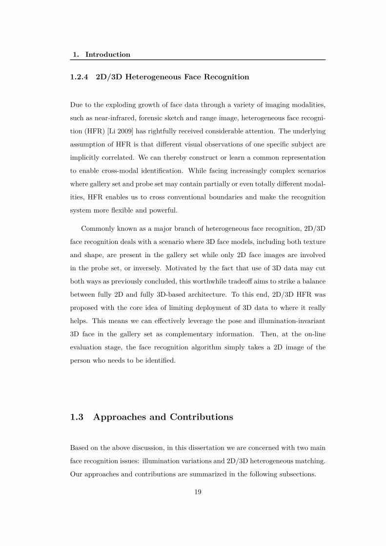
1.2.4 2D/3D Heterogeneous Face Recognition
Due to the exploding growth of face data through a variety of imaging modalities,
such as near-infrared, forensic sketch and range image, heterogeneous face recogni-
tion (HFR) [Li 2009] has rightfully received considerable attention. The underlying
assumption of HFR is that different visual observations of one specific subject are
implicitly correlated. We can thereby construct or learn a common representation
to enable cross-modal identification. While facing increasingly complex scenarios
where gallery set and probe set may contain partially or even totally different modal-
ities, HFR enables us to cross conventional boundaries and make the recognition
system more flexible and powerful.
Commonly known as a major branch of heterogeneous face recognition, 2D/3D
face recognition deals with a scenario where 3D face models, including both texture
and shape, are present in the gallery set while only 2D face images are involved
in the probe set, or inversely. Motivated by the fact that use of 3D data may cut
both ways as previously concluded, this worthwhile tradeoff aims to strike a balance
between fully 2D and fully 3D-based architecture. To this end, 2D/3D HFR was
proposed with the core idea of limiting deployment of 3D data to where it really
helps. This means we can effectively leverage the pose and illumination-invariant
3D face in the gallery set as complementary information. Then, at the on-line
evaluation stage, the face recognition algorithm simply takes a 2D image of the
person who needs to be identified.
1.3 Approaches and Contributions
Based on the above discussion, in this dissertation we are concerned with two main
face recognition issues: illumination variations and 2D/3D heterogeneous matching.
Our approaches and contributions are summarized in the following subsections.
19

1. Introduction
1.3.1 Improving Shadow Suppression for Illumination InvariantFace Recognition
We propose a novel approach for improving lighting normalization to facilitate
illumination-invariant face recognition. To this end, we first build the underlying
reflectance model which characterizes interactions between skin surface, lighting
source and camera sensor, and elaborates the formation of face color appearance.
Specifically, the proposed illumination processing pipeline enables generation of a
Chromaticity Intrinsic Image (CII) in a log chromaticity space which is robust to
illumination variations. Moreover, as an advantage over most prevailing methods,
a photo-realistic color face image is subsequently reconstructed, eliminating a wide
variety of shadows whilst retaining color information and identity details. Experi-
mental results under different scenarios and using various face databases show the
effectiveness of the proposed approach in dealing with lighting variations, including
both soft and hard shadows, in face recognition.
1.3.2 Heterogeneous Face Recognition with Convolutional NeuralNetworks
With the goal of enhancing 2D/3D heterogeneous face recognition, a cross-modal
deep learning method, acting as an effective and efficient workaround, is developed
and discussed. We begin with learning two convolutional neural networks (CNNs) to
extract 2D and 2.5D face features individually. Once trained, they can serve as pre-
trained models for another two-way CNN which explores the correlated part between
color and depth for heterogeneous matching. Compared with most conventional
cross-modal approaches, our method additionally conducts accurate depth image
reconstruction from single color images with Conditional Generative Adversarial
Nets (cGAN), and further enhances recognition performance by fusing multi-modal
matching results. Through both qualitative and quantitative experiments on a
benchmark FRGC 2D/3D face database, we demonstrate that the proposed pipeline
outperforms state-of-the-art performance on heterogeneous face recognition and
ensures a drastically efficient on-line stage.
20

1. Introduction
1.4 Outline
The remainder of this dissertation is organized as follows:
In Chapter 2 we review the representative literature with regard to our re-
search topic. Specifically, the literature covers the fundamentals and approaches
of face recognition with respect to pose variations, lighting variations and 2D/3D
heterogeneous matching.
In Chapter 3 we present our processing pipeline for improving shadow sup-
pression on face images across varying lighting conditions.
In Chapter 4 we present our deep learning-based method for training CNN
models for both realistic depth face reconstruction and effective heterogeneous face
recognition.
In Chapter 5 we conclude this dissertation and propose the perspectives for
future works.
Finally, in Chapter 6 we list our publications.
21

2
Literature Review
Contents2.1 2D Face Recognition Techniques . . . . . . . . . . . . . . . . . 24
2.1.1 Holistic feature based methods . . . . . . . . . . . . . . . . . 24
2.1.2 Local feature based methods . . . . . . . . . . . . . . . . . . 25
2.1.3 Hybrid methods . . . . . . . . . . . . . . . . . . . . . . . . . 27
2.1.4 Deep learning based methods . . . . . . . . . . . . . . . . . . 27
2.2 Illumination Insensitive Approaches . . . . . . . . . . . . . . . 30
2.2.1 Image Enhancement based Approaches . . . . . . . . . . . . . 30
2.2.2 Illumination Insensitive Feature based Approaches . . . . . . 31
2.2.3 Illumination Modeling based Approaches . . . . . . . . . . . 36
2.2.4 3D Model based Approaches . . . . . . . . . . . . . . . . . . 38
2.3 2D/3D Heterogeneous Face Recognition . . . . . . . . . . . . 40
2.3.1 Common subspace learning . . . . . . . . . . . . . . . . . . . 40
2.3.2 Synthesis Methods . . . . . . . . . . . . . . . . . . . . . . . . 44
2.4 Conclusion . . . . . . . . . . . . . . . . . . . . . . . . . . . . . . 47
Both tasks of this dissertation, i.e. face recognition under lighting variations and
heterogeneous scenarios, involve addressing additional challenges specific to their
particular conditions as well as tackling conventional face recognition problems.
Due to the enormous potential of unconstrained face recognition in real-world ap-
plications, these specific issues have been extensively studied and discussed in many
previous researches, offering plenty of inspiration and guidance for our work.
In this chapter, we provide a comprehensive review of the literature on the
related work. We start by introducing the basic and representative 2D based face

2. Literature Review
recognition techniques. Next, we systematically review the illumination-insensitive
approaches and 2D/3D heterogeneous face recognition methods in Section 2.2 and
in Section 2.3, respectively. Finally, some discussions and conclusions are given in
2.4.
2.1 2D Face Recognition Techniques
As previously stated, a large number of 2D feature extraction techniques have been
successfully developed to fulfill the changing requirements in face recognition. Here
we briefly review the most representative methods in four categories: holistic feature
based methods, local feature based methods, hybrid methods and deep learning
based methods.
2.1.1 Holistic feature based methods
In these methods, which are also called appearance-based methods, face images
are globally treated, i.e. no extra effort is needed to define feature points or fa-
cial regions (mouth, eyes, etc. ). The whole face is fed into the FR system as
a pixel matrix and outputs holistic features which lexicographically convert each
image into a high-level representation and learn a feature subspace to preserve the
statistical information of raw image. The two most representative holistic feature
based methods are Eigenfaces related Principal Component Analysis (PCA) [Turk &
Pentland 1991] and Fisherfaces related Linear Discriminative Analysis (LDA) [Bel-
humeur et al. 1997]. It is argued in Eigenfaces that each face image can be ap-
proximated as a linear combination of basic orthogonal eigenvectors computed by
PCA on a training image set (see Fig. 2.1 for details). Motivated from the fact that
Eigenfaces do not leverage the identity information due to the unsupervised learning
with PCA, Fiserfaces was proposed to improve recognition accuracy by maximizing
extra-class variations between images belonging to different people while minimizing
the intra-class variations between those of the same person.
Other holistic feature based methods include the extended version of Eigenfaces
and Fisherfaces, such as 2D-PCA [Yang et al. 2004], Independent Component Anal-
24

2. Literature Review
Figure 2.1: Eigenfaces scheme.
ysis (ICA) [Hérault & Ans 1984] and some of their nonlinear variants, such as Kernel
PCA (KPCA) [Hoffmann 2007] and Kernel ICA (KICA) [Bach & Jordan 2002].
Though these features are easy to implement and can work reasonably well with
good quality images captured under strictly controlled environments, they are quite
sensitive to noise and variations in lighting and expression because even slight local
variations will cause global intensity distributions.
2.1.2 Local feature based methods
Instead of treating face image as a unity, the local feature based methods separate
the whole face into sub-regions and analyze the patterns individually in order to
avoid the local interference. The most commonly used local characteristics are Local
Binary Pattern (LBP) and its variants [Huang et al. 2011].
Initially proposed as a powerful descriptor for texture classification problem,
LBP [Ojala et al. 2002] has rapidly been developed as one of the most popular fea-
tures in face recognition systems. In original face-specific LBP [Ahonen et al. 2006],
25

2. Literature Review
(a)
(b)
Figure 2.2: Schema of LBP operator. (a) An example of LBP encoding schemawith P = 8. (b) Examples of LBP patterns with different numbers of samplingpoints and radius. [Huang et al. 2011]
every pixel of an input image is assigned with a decimal number (called LBP la-
bel) which is computed by binary thresholding its gray level with its P neighbors
sparsely located on a circle of radius R centered at the pixel itself. Using a circular
neighborhood and bilinearly interpolating values at non-integer pixel coordinates
allow any radius and number of pixels in the neighborhood. This encoding scheme is
called LBP operator and denoted as LBP(P,R). Fig. 2.2 show several examples of
LBP encoding patterns. The histogram of these 2P different labels over all pixels in
the face image can then be used as a facial descriptor. More specifically, it has been
shown in [Ojala et al. 2002] that certain patterns contain more information than
others, hence normally only a subset of 2P binary patterns, namely uniform pat-
terns, are used to describe the image. Based on the above LBP methodology, plenty
of its variations have been developed for improved performance in face recognition,
such as Extended LBP [Huang et al. 2007a], Multi-Block LBP [Liao et al. 2007]
and LBP+SIFT [Huang et al. 2010b].
There are also some other approaches that are built upon different local fea-
tures extracted from local components, such as Gabor coefficients [Brunelli & Pog-
26

2. Literature Review
gio 1993], Haar wavelets [Viola & Jones 2004], Scale-Invariant Feature Transform
(SIFT) [Lowe 2004], Local Phase Quantization (LPQ) [Ojansivu & Heikkilä 2008]
and Oriented Gradient Maps (OGM) [Huang et al. 2012]. Due to their additional
information on local regions, local feature based approaches have greatly improved
the performance of holistic feature based face recognition while retaining the ease of
implementation and are widely adopted in most current face recognition systems.
2.1.3 Hybrid methods
This category reasonably leverages the advantages of both holistic and local fea-
tures by using them simultaneously. For example, Cho et al. [Cho et al. 2014]
proposed a coarst-to-fine framework which first applys PCA to identify a test im-
age and then transmits the top candidate images with high degree of similarity
to the next recognition step where Gabor filters are used. This hybrid processing
has certain advantages. First, it can refine the recognition accuracy of PCA-based
global method by introducing a more discriminative local feature. In addition, it
can efficiently filter the images of top candidates with PCA to avoid the heavy
computational load caused by processing all images with Gabor filters.
The other representative methods include SIFT-2D-PCA [Singha et al. 2014],
Multilayer perceptron-PCA-LBP [Sompura & Gupta 2015] and Local Directional
Pattern (LDP) [Kim et al. 2013]. These hybrid methods can effectively improve
the recognition ability by combining both the global and local information of faces.
However, it becomes much more difficult in terms of their implementation when
compared with the two previous approaches.
2.1.4 Deep learning based methods
In recent years, deep learning based methods such as Convolutional Neural Networks
(CNN) have achieved significant progress due to their remarkable ability to learn
concepts with minimal feature engineering and in a purely data driven fashion.
Typically, a CNN is composed of a stack of layers that perform feature extraction
in different ways, e.g. the convolutional layers convolve the input image with filters,
27

2. Literature Review
the rectified linear units layers apply non-linear transformations on filter responses
and the pooling layers spatially pool the resulting values. Each layer goes through a
function to transform itself from one volume of activation to another, this function
is required to be differentiable in order that the weights and bias could be updated
according to the gradient during the back-propagation. CNNs and ordinary neural
networks (NN) are quite alike since they both consist of neurons that have learnable
weights and biases, but they differ from NNs in two ways: (1) CNNs use convolution
instead of general matrix multiplication in at least one of their layers, (2) the number
of parameters in CNNs is significantly reduced in comparison with fully connected
NNs due to weights sharing.
The application of CNN in face recognition can date back to the 90s, Lawrence
et al. [Lawrence et al. 1997] first implemented a basic CNN architecture, as illus-
trated in Fig. 2.3, to address the face recognition problem. However, very few
attempts have been made to improve the use of CNN for a long period, this slow
development is in relation with three problems: 1) Lack of enough training sam-
ples. A CNN architecture usually contains a large amount of parameters, hence
adequate training samples are required for an accurate model fitting, which were
hardly available before the collection of large-scale databases in recent years. For
example, in [Lawrence et al. 1997] the network is trained on the ORL dataset which
only contains 200 training images. 2) Limited computational power. The numerous
parameters in CNN not only cause high demand for data, but also pose challenges
for hardwares. The investigation of deep CNNs would not be feasible with low-
performance computational resources. 3) Immature technology. The complexity of
CNN makes it highly sensitive to architecture details and training techniques, e.g.
the choice of activation function and the problem of overfitting.
Not surprisingly, as the large-scale datasets and high-performance graphic cards
become increasingly popular, the capacities of CNNs to learn spatially local correla-
tion from raw images and to compose lower-level features into higher-level ones are
immediately recalled. Moreover, the improvements in CNN training techniques, e.g.
using rectified linear unit (ReLU) instead of traditional Sigmoid function for non
linearity [Nair & Hinton 2010] and implementing dropout layers to avoid overfit-
28

2. Literature Review
Figure 2.3: The first convolutional neural network for face recognition [Lawrenceet al. 1997].
Figure 2.4: Outline of the Deepface architecture proposed in [Taigman et al. 2014].
ting [Srivastava et al. 2014], have made the CNN-based approaches more powerful.
The extraordinary success was first achieved in 2012 on the ImageNet object clas-
sification challenge [Russakovsky et al. 2015] by famous CNN architectures [Gu
et al. 2015], such as AlexNet, VGGNet, GoogleNet, ResNet, etc. As for the ap-
plication of CNNs in face recognition, 2014 was a breakthrough year which has
witnessed the emergence of three famous CNN architectures, i.e. Deepface [Taig-
man et al. 2014], DeepID [Sun et al. 2014b] and DeepID2 [Sun et al. 2014a]. On
the Labeled Faces in the Wild (LFW) benchmark which contains 13,233 images
from 5,749 identities, these three CNN based methods achieved 97.35%, 97.45%
and 99.15% for face verification task, respectively. Fig. 2.4 illustrates an example
of the Deepface architecture. Comparing the two architectures in Fig. 2.3 and Fig.
2.4, we can infer that modern CNNs can reasonable extract more discriminative
high-level representations from numerous face images with larger size by learning
a deep network with a large number of parameters (more than 120 millions in
Deepface).
29

2. Literature Review
Currently, the state-of-the-art results on LFW was achieved by FaceNet [Schroff
et al. 2015] (99.63%) and some commercial systems such as Baidu [Liu et al. 2015]
(99.77%). These researches generally combined various techniques to improve the
classification ability of their networks, e.g. training dataset with larger scale, multi-
CNNs based on different facial regions and more effective metric learning such as
triplet loss [Schroff et al. 2015]. Meanwhile, there are also several methods focusing
on improving the CNNs from other perspectives, such as using sparse networks
with fewer parameters instead of the dense ones [Sun et al. 2016] and efficiently
enhancing the discriminative power of CNNs with center loss [Wen et al. 2016].
2.2 Illumination Insensitive Approaches
Over the years, a surge of qualitative and quantitative studies on illumination in-
variant research have been put forward by reason of their suitability and efficacy
in face analysis. These techniques could be roughly divided into three categories
according to their diverse theoretical backgrounds: image enhancement based meth-
ods, invariant feature extraction methods and 3D model based methods.
2.2.1 Image Enhancement based Approaches
The image enhancement based pre-processing methods used to be common in early
algorithms. They attempt to globally or locally redistribute some specific charac-
teristics of the original face image, e.g. the dynamic range of the intensity values
and the shape of the histogram, in a predefined representation. These tasks are gen-
erally achieved by applying simple gray-scale intensity adjustments to compensate
the illumination variations.
Histogram Equalization (HE) and Histogram Matching (HM) [Pizer et al. 1987]
initiated these methods by adopting different image processing methods at the
histogram level: HE increases the global contrast by flattening the histogram while
HM matches the histogram of target image to a specified histogram. Adini Shan et
al. [Shan et al. 2003] developed Gamma Intensity Correction (GIC) for normalizing
the overall image intensity at the given illumination level by introducing an intensity
30

2. Literature Review
mapping: G(x, y) = cI(x, y)1/γ where c is a gray stretch parameter and γ is the
Gamma coefficient. Instead of normalizing the illumination globally, Xie and Lam
[Xie & Lam 2006] proposed a novel local normalization (LN) method to effectively
and efficiently eliminate the effect of uneven illumination. In this method, a human
face is treated as a combination of a sequence of small and flat facets, LN then
processes the image in order that the intensity value is of zero mean and with unit
variance within each facet.
Notwithstanding their ease of implementation and the apparent beneficial effects
on lighting normalization, these methods fail to further satisfy the more and more
rigorous demands on accuracy because they do not take into account the in-depth
image formation principles, which means that they simply average the distribution
of intensities or histograms and thus remain prone to complicated lighting condi-
tions, e.g. soft shadows, hard shadows or highlights.
2.2.2 Illumination Insensitive Feature based Approaches
In view of the deficiency of photometric normalization based approaches, the illu-
mination invariant feature extraction methods have been extensively investigated.
To be more specific, as stated in [Chen et al. 2000] that there are no strictly
illumination-invariant features for objects with a Lambertian surface, these methods
can more appropriately be termed as illumination insensitive as opposed to illumina-
tion invariant. Known as a mainstream solution against lighting variations which is
widely employed in most current face recognition systems, the related approaches
can be further categorized into three classes: image gradient based approaches,
Retinex theory based approaches and frequency domain based approaches.
Image gradient based approaches. The principle of image gradient or edge
based approaches is to extract the gray-level gradients or edges from the face image
and study their lighting-insensitive characteristics. This is theoretically plausible
because the gradients or edges effectively emphasize high-frequency information
instead of low-frequency one which is easily sensitive to global lighting variations
[Chen et al. 2000]. Furthermore, the gradient domain explicitly reflects the local
relationships between neighboring pixels, which makes it capable of highlighting the
31

2. Literature Review
underlying intrinsic structure of images [Makwana 2010].
In [Kanade 1977], Kanade first started the analysis of how different edge-
detection operators, including the Laplacian operator, the Robertz operator and the
maximum of differences for 3×3 window, impact on face recognition performance.
Some early methods [Duc et al. 1999,Lyons et al. 1999,Liu & Wechsler 2001] con-
volved facial images with Gabor-like filters in order to enhance edges. Line Edge
Map (LEM) [Gao & Leung 2002] was proposed to group edge pixels into line seg-
ments, and a revised Hausdorff Distance is introduced to perform the similarity
measurement between two edge maps. While achieving significant improvement
compared with traditional methods such as Eigenface, the line edge map based
methods inevitably lack the information encoded in the intensity shade and suffer
from generating similar results for different faces. Therefore, gradient-based meth-
ods were studied in order to retain more identity-specific information. Wei and
Lai [Wei & Lai 2004] proposed the relative image gradient feature RIG(x, y) for
robust face recognition, which is defined as:
RIG(x, y) =|∇I(x, y)|
max(u,v)∈W (x,y)
|∇I(u, v)|+ c(2.1)
where I(x, y) is the image intensity function, the notation ∇ denotes the gradient
operator that takes the partial differentiation along x and y directions, W (x, y) is
a local window centered at the location (x, y), and c is a positive constant used to
avoid dividing by zero. More recently, Zhang et al. [Zhang et al. 2009b] proposed a
novel illumination-insensitive feature GF , namely Gradientfaces, by computing the
ratio between gradients of a smoothed image I in the x, y directions:
GF (x, y) = arctan(Iy−gradient(x, y)
Ix−gradient(x, y)
), G(x, y) ∈ [0, 2π) (2.2)
Similar processing could be seen in Weberface proposed in [Wang et al. 2011], which
instead computes the ratio of the local intensity variation to the background of a
given image to obtain illumination invariant representations. Given a face image
32

2. Literature Review
I(x, y), the corresponding Weberface, denoted by WF , can be formulated as follows:
WF (x, y) = arctan
α∑i∈A
∑j∈A
I(x, y)− I(x− i∆x, y − j∆y)
I(x, y)
(2.3)
in which A = −1, 0, 1 and α is a parameter for adjusting (magnifying or shrinking)
the intensity difference between neighboring pixels.
Despite the improvement of performance by using these methods, Adini et
al. [Adini et al. 1997] have demonstrated that Gabor-like filters, edge maps and
image derivatives are insufficient to overcome the illumination problem because
such processes mainly take place in the primary visual cortex and remain sensitive
to lighting directions and noise.
Retinex theory based approaches. The term retinex was the theory of hu-
man color vision proposed by Land and McCann [Land & McCann 1971] which tries
to explain the basic principles governing the process of image formation. According
to the retinex theory, an image I(x, y) can be decomposed into two components,
which are the luminance L(x, y) and the reflectance R(x, y), as shown in Eq. 2.4:
I(x, y) = R(x, y)L(x, y) (2.4)
Here, the luminance L(x, y) varies according to the different illuminations , while
the reflectance R(x, y) relates to the characteristics of the face and is dependent
on the reflectivity (or albedo) of the face skin. It is therefore obvious that the
R(x, y) acts as an illumination invariant feature of the face image. Furthermore, as
evidenced in [Land & McCann 1971], the luminance is assumed to change slowly
across a face image, which implies that it can be estimated as a smoothed version of
the image. To this end, a number of smooth filters and methods have been proposed
in the literature.
Jobson et al. [Jobson et al. 1997a] developed the single scale retinex (SSR)
algorithm which applied a single Gaussian function F (x, y) to smooth the image
33

2. Literature Review
and estimated the reflectance RSSR(x, y) in the log space:
RSSR(x, y) = log(I(x, y))− log(I(x, y) ∗ F (x, y)), F (x, y) = C exp(−x2 + y2
2σ2)
(2.5)
where C is a normalization factor and σ denotes the filter standard deviation.
However, the choice of the right scale σ for F (x, y) is crucial and difficult in SSR
algorithm. To avoid this problem, the authors [Jobson et al. 1997b] extended their
smooth filter in SSR to a multi scale form, i.e. multi-scale retinex (MSR), where
the output reflectance RMSR(x, y) is a weighted sum of several SSR outputs with
different Gaussian filters:
RMSR(x, y) =N∑
n=1
ωnRn =N∑
n=1
ωn[log(I(x, y))− log(I(x, y) ∗ Fn(x, y))] (2.6)
where N is the number of scales, ωn is the weight of each scale, Fn(x, y) relates to
a specific F (x, y) in Eq. 2.5 with Cn and σn.
Based on the assumption of treating face as an ideal class of object, i.e. different
faces share the same shape but differ in the skin albedo, Shashua and Riklin-Raviv
[Shashua & Riklin-Raviv 2001] proposed a novel approach called quotient image
(QI). The quotient image is defined as the ratio between one face image and a linear
combination of three prototype images based on the Lambertian model and is proved
to be illumination free. However, the computation of QI requires a bootstrap set and
assumes a similar shape for faces, which remain strong constraints for its broader
use in robust face recognition. Then, Wang et al. [Wang et al. 2004] developed a
self quotient image (SQI) based method to improve the QI method by replacing the
prototype images with a smoothed version of test image itself. Additionally, instead
of using isotropic smoothing as in MSR [Jobson et al. 1997b], anisotropic smoothing
filter is applied in SQI to avoid the halo effect around edge region. This method
is simple and requires no image registration, however, the weighed Gaussian filter
they used has trouble keeping sharp edges in low frequency illumination fields. To
enhance the edge preserving capacity, Chen et al. [Chen et al. 2005] proposed the
total variation based quotient image (TVQI) by introducing the idea of TV + L1
34

2. Literature Review
model: minimizing the total variation of the output cartoon while subject to an L1-
norm fidelity term. In this approach, the estimation of luminance u was achieved
by minimizing the following function:
u = arg minu
∫Ω|∇u(x)|+ λ|f(x)− u(x)|dx (2.7)
where f is the original face image and Ω covers all pixels in f . Once u is optimized,
the TVQI can be represented by TV QI = f/u.
Frequency domain based approaches. According to the previously adopted
assumption, the lighting condition changes slowly except for hard shadows and
specularities on the face. Consequently, illumination variations mainly lie in the
low-frequency band, leading to these methods which involve compensating lighting
variations in specific domains related to frequency transformations.
Du and Ward [Du & Ward 2005] used wavelet decomposition to transform an
image into its low/high frequency domains and then manipulated different band
coefficients separately, a normalized image was finally obtained from the modified
coefficients by inverse wavelet transform. Compared with aforementioned histogram
equalization, this approach has the advantage of taking into account both contrast
and edge enhancement simultaneously. Similarly, Zhang et al. [Zhang et al. 2009a]
proposed the multiscale facial structure representation (MFSR) to reduce the effect
of illumination by wavelet-based denoising techniques and soft thresholding. Chen
et al. [Chen et al. 2006b] performed a discrete cosine transform (DCT) in the log-
arithm domain, the illumination variations under different lighting conditions are
significantly reduced after truncating an appropriate number of low-frequency DCT
coefficients.
Besides the above methods based on various processing principles, the reason-
able combination of different pre-processing methods likewise remains a solution.
The most representative fusion strategy is the integrative pre-processing chain per-
formed by Tan and Triggs (TT) [Tan & Triggs 2010] which successively merged
Gamma correction, Difference of Gaussian filtering, optional masking and contrast
equalization. According to the results of comparative study in [Han et al. 2013],
35

2. Literature Review
Figure 2.5: Visual comparison for face images normalized with different illuminationpreprocessing methods on databases with controlled and less-controlled lighting[Han et al. 2013].
this simple and efficient image pre-processing chain effectively outperformed most
lighting processing methods, demonstrating the robustness of this fusion scheme.
Fig. 2.5 qualitatively compare the illumination normalization quality of different
preprocessing methods on two benchmark face databases, i.e. Yale B extended and
FRGC Ver2.0 face databases.
All these illumination insensitive feature based approaches achieved impres-
sive performance on normalizing global illuminations and removing soft shadows,
yet encountered problems with hard-edged cast shadows especially caused by self-
occlusion as in the area of nasal alar. Meanwhile, these techniques can not be
extended to color space, resulting in limited applications in real world.
2.2.3 Illumination Modeling based Approaches
Other than extracting the illumination insensitive features from facial images, an-
other train of thought is to model face images under varying lighting conditions.
Given the training images with different illuminations, the conventional statistical
methods such as PCA and LDA treat lighting as an intra-class variance and learn
a subspace to cover possible lighting variations. Moreover, various physical models
36

2. Literature Review
have been proposed to achieve more illumination-specific modeling. We categorize
and present these methods as follows.
Subspace-based approaches aim to construct a linear subspace which covers
the variations of possible illumination. This concept was first investigated by Halli-
nan [Hallinan et al. 1994] who has shown empirically that there exists a reasonably
good 5-dimensional approximation of the face images under varying lighting con-
ditions. To obtain these basis images, this method densely sampled images under
different point light sources I(θ, ϕ) where θ and ϕ denote the longitude and the
latitude respectively, the basis images Sk are then computed by PCA in order that
cI(θi, ϕj) ≈∑
k αijkSk with a scale factor c.
Shashua [Shashua 1997] proposed the photometric alignment method to con-
struct a 3D linear subspace. Assume that a face is Lambertian, given three pictures
of one identity I1, I2, I3 from linearly independent light source directions s1, s2, s3,
this method is then based on a result that any other image I of the face taken from
a novel setting of light sources can be simply represented by a linear combination
of the three pictures, i.e. I = α1I1+α2I2+α3I3. The photometric problem of face
recognition is therefore reduced to the problem of determining the linear coefficients
α1, α2, α3 for each enrolled identity. Once the coefficients are solved, if I is of the
same identity, then I and the synthesized image I ′ = α1I1 + α2I2 + α3I3 should
perfectly match. Shashua claimed that attached shadows in the novel image, or
shadows in general in the model images, do not have significant adverse effects on
the photometric alignment scheme. However, the cast shadows cannot be modeled
in this framework.
Through analyzing the reflectance function of the convex Lambertian surface
in spatial-frequency domain, Basri and Jacob [Basri & Jacobs 2003] proved that
a convex Lambertian object obtained under a large variety of lighting conditions
can be approximated by a 9D linear subspace based on a spherical harmonic rep-
resentation. To be more precise, the lighting function l can be written as sum of
37
2. Literature Review
spherical harmonics as in Eq. 2.8.
l =2∑
n=0
n∑m=−n
lnmYnm (2.8)
where lnm is amplitude of light at order n and Ynm is an nth order harmonic. This
conclusion was contemporarily made by Ramamoorthi and Hanrahan [Ramamoor-
thi & Hanrahan 2001].
Illumination cone was proposed by Belhumeur and Kriegman [Belhumeur &
Kriegman 1996] which takes both pose variations and illumination variations into
account. The basic thought behind this approach is that all images of a convex
object from a fixed viewpoint but illuminated by an arbitrary number of distant
point sources form a convex illumination cone in Rn where n denotes the number
of pixels in the image. Hence each human face could be regarded as the collection
of illumination cones under different poses. Theoretically, a single illumination
cone can be constructed from as few as three images of an object under varying
illuminations. Georghiades [Georghiades et al. 2001] exploited the illumination cone
technique to implicitly recover the shape and albedo from seven images per person
captured under controlled lighting. The effectiveness in face recognition task of this
photometric stereo algorithm has been validated on the Yale face dataset B.
Inspired by the analytic results achieved in this theory, some extensive researches
have been carried out to further enhance the performance. For example, Lee et
al. [Lee et al. 2001] combined the spherical harmonics and the illumination cone
to find nine optimal point lights for the construction of basis images. However,
despite its outstanding performance in face recognition task, the application of
illumination cone based methods is greatly limited by their specific requirements
for training images.
2.2.4 3D Model based Approaches
With the ever-advancing development of 3D data acquisition and application tech-
nologies, many researchers turned their attention to 3D aided lighting processing
methods due to their potential capabilities to overcome the inherent limitations and
38

2. Literature Review
drawbacks of 2D based approaches.
Proposed as an analysis-by-synthesis framework, 3D statistical model provides
a sophisticated solution to the issue of face shape estimation by leveraging the prior
information collected on registered faces. The best known work in this field is the
3D morphable model (3DMM) of Blanz and Vetter [Blanz & Vetter 1999,Blanz &
Vetter 2003]. The 3DMM fitting algorithm argued that both shape and texture of
any realistic human face could be constructed by a linear combination of a set of
examples. The challenge of fitting statistical model to unseen images essentially
amounts to solving a highly complex nonlinear minimization problem which re-
quires estimation of various parameters shape coefficients, texture coefficients and
22 rendering parameters with respect to imaging environment. The performance of
3DMM was tested on the publicly available CMU-PIE database and the recognition
rate varies from 89.0% to 95% for front, side and profile view.
Other 3D model based methods are subsequently investigated to account for
the lighting variations in face recognition. For example, a publicly available 3D
morphable face model containing 200 textured 3D scans - the Basel Face Model
(BFM) [Paysan et al. 2009] - was constructed to facilitate the widespread use of
3DMM. Zhang and Samaras [Zhang & Samaras 2006] have shown that the combina-
tion of a morphable model and spherical harmonic illumination representation [Basri
& Jacobs 2003] facilitates recognition for images with variations of both pose and
illumination. This idea was further strengthened and extended in the Spherical
Harmonic Basis Morphable Model (SHBMM) [Wang et al. 2009] for face relight-
ing from a single Image under arbitrary unknown lighting conditions. Based on
physical lighting models, Zhao et al. [Zhao et al. 2014] decomposed lighting effects
using ambient, diffuse, and specular lighting maps and estimated the albedo for
face images with drastic lighting conditions.
3D based lighting independent methods are powerful and accurate compared
with 2D based ones. However they are easily confined to data acquisition and
the unavoidable high computational cost. Even we can compromise by considering
only 2D images and normalizing their lightings using 3D models, data registration
between 2D and 3D remains likewise an inconvenience.
39

2. Literature Review
2.3 2D/3D Heterogeneous Face Recognition
The main challenge of matching two modalities with underlying correlation yet
large appearance differences lies in the search of common matching domain. Over
the past decade, a few attempts have been made to propose impressive 2D/3D
heterogeneous face recognition algorithms. These methods, categorized by how the
common space is constructed, are recapitulated below.
2.3.1 Common subspace learning
Learning a common subspace is a conventional and classical approach to address the
cross domain recognition problem. The core idea is to find a discriminative common
feature space where the mapped representations of both 2D and 3D modalities could
be directly compared. To ensure the correlation between these modalities, several
projection techniques have been proposed, among which the canonical correlation
analysis is one of the best known.
Canonical Correlation Analysis (CCA) [Hotelling 1936] is a suitable and domi-
nant multivariate analysis method especially useful for exploring the relationships
among these variables. Generally, this technique relates two sets of variables by
maximizing the correlation between them in the CCA subspace. Given N pairs
of samples (xi, yi) of (X,Y ), i = 1, ..., N , where X ∈ Rm, Y ∈ Rn with the mean
value of zero, the goal of CCA is to find two sets of projection directions, ωx and
ωy to maximize the correlation between the two projections ωTxX and ωT
y Y where
T denotes the transpose. In the context of CCA, these two projections are also
referred as canonical variants. Formally, the two directions can be estimated by
maximizing:
ρ =E[ωT
xXYTωy]√
E[ωTxXX
Tωx]E[ωTy Y Y
Tωy](2.9)
where E[·] denotes the empirical expectation. Note that the covariance matrix of
(X,Y ) can be written as:
C(X,Y ) = E
[(X
Y
)(X
Y
)T]= E
[(Cxx
Cxy
)(Cyx
Cyy
)T]
(2.10)
40

2. Literature Review
Figure 2.6: Patch based CCA for 2D-3D matching proposed in [Yang et al. 2008].
where Cxx and Cyy are within-sets covariance matrices, Cxy and Cyx are between-
sets covariance matrices with Cxy = CyxT . Therefore, the objective function ρ could
be rewritten as:
ρ =ωTxCxyωy√
ωTxCxxωxωT
y Cyyωy
(2.11)
the maximum canonical correlation is the maximum of ρ with respect to ωx and
ωy. Once ωx and ωy are learnt, to test new pairs of variables X ′ and Y ′, we first
map them into CCA subspace with x′ = ωTxX
′ and y′ = ωTy Y
′, the similarity score
can then be computed as:
Score(x′, y′) =x′ · y′
∥x′∥ · ∥y′∥(2.12)
CCA has been widely used in heterogeneous matching due to its high efficiency
and robustness. These methods differ from each other mainly in terms of their
extracted features before the mapping into common subspace. Yang et al. [Yang
et al. 2008] initiated the use of CCA regression in 2D-3D face recognition between
eigenfaces of 2D texture images and 2.5D range images. Additionally, they further
investigated a patch based extension of this framework, which is illustrated in Fig.
2.6.
Inspired by the above work, Huang et al. [Huang et al. 2009,Huang et al. 2010a]
first extracted LBP histograms for texture images and range images respectively, a
41

2. Literature Review
linear CCA was then introduced to learn the mapping between the LBP faces from
two modalities. This work was subsequently extended in [Huang et al. 2012] by
proposing an illumination-robust representation, namely Oriented Gradient Map
(OGM), which is computed by Eq. (2.13)
ρR(x, y) = [ρR1 (x, y), ..., ρRO(x, y)]
t, (2.13)
where ρRo (x, y) is the gradient norm within the radius of the given neighborhood
area R of the input image in a direction o at every pixel location (x, y). The
OGM features are advantageous over eigenfaces and LBP descriptors in that they
simulates the response of complex neurons to gradient information within a given
neighborhood, and are able to describe both local texture changes and local ge-
ometry variations from 2D/2.5D image pairs. The experiments were performed on
the FRGC v2.0 database with a gallery of 466 scans and a probe of 3541 images.
The proposed 2D-3D face matching achieved a recognition accuracy of 94.04% in
contrast to 93.90% with 2D-2D matching method, highlighting the effectiveness of
this heterogeneous pipeline. Moreover, after fusing these two scenarios in the score
level, the result has been increased considerably to 95.37%.
The success of applying CCA in cross-modality matching naturally motivates
the exploitation of its variants with more powerful ability to learn good projections.
Wang et al. [Wang et al. 2014] adopted a single-layer network based on Gaussian
Restricted Boltzmann Machines (GRBM) to extract latent features over two dif-
ferent modalities (see Fig. 2.7). More importantly, several different correlation
schemes for learning the common subspace are further evaluated, including CCA,
the regularized CCA and the regularized kernel CCA [Hardoon et al. 2004]. Specif-
ically, the regularized CCA (rCCA) adds the regularization coefficients λx, λy to
each data set to stabilize the solution, the Eq. 2.11 then becomes:
ρ =ωTxCxyωy√
ωTx (Cxx + λxI)ωxωT
y (Cyy + λyI)ωy
(2.14)
Furthermore, considering that CCA may not be extract useful descriptors of the
42

2. Literature Review
(a) (b)
Figure 2.7: The 2D-3D face recognition framework proposed in [Wang et al. 2014].(a): Illustration of training and testing scheme. (b): Illustration of principal com-ponents of the scheme.
data because of its linearity, the regularized kernel CCA (rKCCA) offers an alterna-
tive solution by first projecting the data into a higher dimensional feature space by
introducing kernel functions. The experimental results on the FRGC v2.0 database
proved the superiority of using rKCCA instead of CCA and rCCA.
Besides the numerous studies based on CCA and its variants, some other com-
mon subspace learning methods are investigated as well. By adding the Laplacian
penalty constraint for the multiview feature learning, Jin et al. [Jin et al. 2014]
first proposed the Multiview Smooth Discriminant Analysis (MSDA) to find a com-
mon discriminative feature space which can fully utilize the underlying relationship
of features from different views. Then a recent popular algorithm named Extreme
Learning Machine (ELM) is adopted in training the single hidden layer feed-forward
neural networks (SLFNs) to speed up the learning phase of the classifier. The com-
prehensive framework is shown in Fig. 2.8.
The common subspace learning based methods can successfully construct dis-
criminative common feature space by using a variety of projection techniques. How-
ever, most of these transformations are linear and shallow, which therefore makes
them partially restricted for nonlinear and complicated representations in real case.
43

2. Literature Review
Figure 2.8: Intuitive explanation of the Multiview Smooth Discriminant Analysisbased Extreme Learning Machines (ELM) approach [Jin et al. 2014].
2.3.2 Synthesis Methods
Unlike constructing a discriminative common subspace, the synthesis methods offer
a more intuitive solution by synthesizing one modality based on the other. The syn-
thesized results can then be directly used in conventional single modality matching.
These approaches are relatively straightforward and easily comparable, yet critically
dependent on the fidelity and robustness of the synthesis method.
As illustrated in Fig. 2.9, Toderici et al. [Toderici et al. 2010] leveraged the
3D mesh and 2D texture in the gallery set to synthesize 2D images which can be
matched directly with the 2D images in the probe. Specifically, the synthesized
gallery texture and the probe texture are required to be consistent in the lighting
conditions for better performance. A novel method for bidirectional relighting in
3D-2D face recognition under large illumination changes is therefore presented in
this paper. To achieve this, in the enrollment phase they fit an Annotated Face
Model (AFM) [Kakadiaris et al. 2007] to the raw 2D+3D data using a subdivision-
based deformable framework and represent the fitted AFM as a geometry image. In
the recognition phase, the enrolled AFM is first registered to the 2D probe image
for pose alignment and visibility map computation. Then the enrolled 2D gallery
44

2. Literature Review
Figure 2.9: Overview of the reference 3D-2D face recognition system with illumi-nation normalization between probe and gallery textures [Toderici et al. 2010].
texture is bidirectionally relighted to match the 2D probe texture. The matching
score is eventually computed using the relit gallery texture and the probe texture.
This approach was further extended and refined in [Zhao et al. 2014, Kakadiaris
et al. 2016].
Zhang et al. [Zhang et al. 2014] rendered images in various poses by transforming
the 3D mesh and lifting the 2D texture in the gallery set. These generated images
serve as input with labels to supervise the learning of a random forest (RF) for
head pose estimation. For an unseen probe image, the estimated pose value from
the trained RF is considered as a reasonable initialization for 3DMM which will
normalize the head pose to frontal view. The matching can thus be conducted
between frontal gallery images and normalized probe images.
Note that the above methods can be roughly categorized into two classes: one
renders the 2D+3D data in gallery to synthesize images which are close to probe
images while another normalizes the imaging conditions, e.g. pose and illumination,
to make both views look similar. An interesting study [Wu et al. 2016] was recently
released to present an extensive evaluation of these two frameworks. Specifically, the
pose normalization and pose rendering based methods are compared in an empirical
manner. The authors concluded that the rendering-based methods perform better
than the normalization-based methods when a face has a large deviation from frontal
pose while the latter can achieve better alignment of facial texture.
45

2. Literature Review
Compared with the various methods on synthesizing 2D images from 3D face
models, very few attempts have been made in a reverse way, i.e. by matching 3D
galley face with reconstructed 3D face from the 2D probe texture. This is mainly
due to the assumption that the gallery contains both 2D and 3D data. Under this
assumption, synthesizing 2D images is straightforward and simple, while the shape
reconstruction from a single 2D image remains an ill-posed problem. However, in
many practical cases the gallery may only contain 3D face shape without texture
information, therefore highlighting the importance of shape reconstruction, or depth
estimation.
A number of prevailing approaches have been devoted to address this problem
based on shape-subspace projections, where a set of 3D prototypes are fitted by
adjusting corresponding parameters to a given 2D image. Most of them, e.g. [Pi-
otraschke & Blanz 2016] and [Roth et al. 2016], are derived from 3DMM [Blanz
& Vetter 2003] and Active Appearance Models [Matthews et al. 2007]. Alternative
models were afterwards proposed as well which follow the similar processing pipeline
by fitting 3D models to 2D images through various face collections or prior knowl-
edge. For example, Gu and Kanade [Gu & Kanade 2006] fit surface 3D points and
related textures together with the pose and deformation estimation. Kemelmacher-
Shlizerman et al. [Kemelmacher-Shlizerman & Basri 2011] considered the input
image as a guide with a single reference model to achieve 3D reconstruction. In
recent work of Liu et al. [Liu et al. 2016], two sets of cascaded regressors are im-
plemented and correlated via a 3D-2D mapping iteratively to solve face alignment
and 3D face reconstruction simultaneously. Likewise, using generic model remains
a decent solution as well for 3D face reconstruction from stereo videos, as presented
in [Chowdhury et al. 2002,Fidaleo & Medioni 2007,Park & Jain 2007]. Given ade-
quate and appropriate 3D prototypes, the strikingly accurate reconstruction results
have been reported in the above researches.
It is worth noticing that among all these 2D-3D heterogeneous face recogni-
tion researches, some take complete 3D face model [Toderici et al. 2010, Zhang
et al. 2014, Kakadiaris et al. 2016], such as dense point cloud and vertex-
face mesh, while the others only process pseudo-3D [Huang et al. 2012, Jin
46
2. Literature Review
et al. 2014, Wang et al. 2014], also known as 2.5D image, for heterogeneous com-
parison with ordinary photographic image. In recent years, some RGB-D databases
[Min et al. 2014, Goswami et al. 2014] and corresponding approaches [Goswami
et al. 2016,Boutellaa et al. 2015,Song et al. 2015,Cardia Neto & Marana 2015] have
been proposed as well, but the performance are greatly limited by the low resolu-
tion images captured in RGB-D devices like Kinect. Using full 3D model could be
advantageous to handle pose variations other than frontal pose due to its capacity
of transforming face model in 3D space to fit the real pose. Nevertheless, 2.5D
based methods hold advantage with its ease of implementation and outstanding
performance when dealing with frontal pose scenarios as considered in many large
3D face datasets, such as FRGC, BU3D and Bosphorus. In addition to its effi-
ciency and effectiveness, the fact that 2.5D still retains the characteristic of acting
as an image endows 2.5D based methods with more flexibility and attractiveness
for combination with other powerful 2D based techniques.
2.4 Conclusion
Through this chapter, an up-to-date literature review of both illumination process-
ing approaches and 2D-3D heterogeneous face recognition approaches is extensively
conducted. For each research topic, the most representative approaches and their
corresponding performance have been presented and discussed.
Other than analyzing the advantages and drawbacks of these methods, we also
provide the main concepts behind our own work in this thesis, which are:
• Building a comprehensive imaging formation model with respect to the source
lighting, skin surface and camera sensor. Suppressing shadows based on this
physical model to improve the face recognition performance against illumina-
tion variations.
• Combining common subspace learning method and synthesis method to build
a multi-modality matching framework for 2D-3D heterogeneous face recogni-
tion.
47

2. Literature Review
• Applying the powerful convolutional neural networks to extract discriminative
facial descriptors and to reconstruct depth images from texture images.
48

3
Improving Shadow Suppression
for Illumination Robust Face
Recognition
Contents3.1 Introduction . . . . . . . . . . . . . . . . . . . . . . . . . . . . . 50
3.2 Skin Color Analysis . . . . . . . . . . . . . . . . . . . . . . . . . 53
3.2.1 Reflectance Model: Lambert vs. Phong . . . . . . . . . . . . 53
3.2.2 Specular Highlight Detection . . . . . . . . . . . . . . . . . . 54
3.2.3 Skin Color Formation . . . . . . . . . . . . . . . . . . . . . . 56
3.3 Chromaticity Invariant Image . . . . . . . . . . . . . . . . . . . 58
3.3.1 Skin Model in Chromaticity Space . . . . . . . . . . . . . . . 58
3.3.2 Chromaticity Invariant Image Generation . . . . . . . . . . . 59
3.3.3 Entropy based Lighting Normalization . . . . . . . . . . . . . 62
3.3.4 Global Intensity Regularization . . . . . . . . . . . . . . . . . 64
3.4 Shadow-free Color Face Recovery . . . . . . . . . . . . . . . . 64
3.4.1 In-depth Analysis of 1D Chromaticity Image . . . . . . . . . 64
3.4.2 Shadow-Specific Edge Detection . . . . . . . . . . . . . . . . 66
3.4.3 Full Color Face Image Reconstruction . . . . . . . . . . . . . 67
3.5 Experimental Results . . . . . . . . . . . . . . . . . . . . . . . . 69
3.5.1 Databases and Experimental Settings . . . . . . . . . . . . . 69
3.5.2 Visual Comparison and Discussion . . . . . . . . . . . . . . . 73
3.5.3 Identification Results on CMU-PIE . . . . . . . . . . . . . . . 77

3. Improving Shadow Suppression for Illumination Robust FaceRecognition
3.5.4 Verification Results on FRGC . . . . . . . . . . . . . . . . . . 80
3.6 Conclusion . . . . . . . . . . . . . . . . . . . . . . . . . . . . . . 83
3.1 Introduction
Face analysis has received a great deal of attention due to the enormous devel-
opments in the field of biometric recognition and machine learning. Beyond its
scientific interest, face analysis offers unmatched advantages for a wide variety of
potential applications in commerce and law enforcement as compared to other bio-
metrics, such as easy access or avoidance of explicit cooperation from users [Zhao
et al. 2003]. Nowadays conventional cases have attained quasi-perfect performance
in a highly constrained environment wherein poses, illuminations, expressions and
other non-identity factors are strictly controlled. However these approaches suffer
from a very restricted range of application fields due to non-ideal imaging environ-
ments frequently encountered in practical cases: the users may present their faces
not with a neutral expression, or human faces come with unexpected occlusions such
as sunglasses, or even the images are captured from video surveillance which can
gather all the difficulties such as low resolution images, pose changes, lighting con-
dition variations, etc. In order to be adaptive to these challenges in practice, both
academic and industrial research understandably shift their focus to unconstrained
real-scene face images.
Compared with other nuisance factors such as pose and expression, illumination
variation impinges more upon many conventional face analysis algorithms which as-
sume a normalized lighting condition. As depicted in Fig. 3.1, the lighting condition
can be fairly complicated due to numerous issues: the intensity and direction of the
lighting, the overexposure and underexposure of the camera sensor, just to name
a few. Not only that, but it has already been proven that in face recognition, dif-
ferences caused by lighting changes could be even more significant than differences
between individuals [Adini et al. 1997]. Therefore, lighting process, either light-
ing reconstruction (re-lighting) or lighting normalization (de-lighting), turns out to
50

3. Improving Shadow Suppression for Illumination Robust FaceRecognition
(a) (b) (c) (d)
Figure 3.1: An example of varying lighting conditions for the same face. (a) Frontlighting; (b) Specular highlight due to glaring light coming from right side; (c) Softshadows and (d) hard-edged cast shadow.
be crucially important for exploring illuminant-invariant approaches. Considering
that the reconstruction of differing lighting normally requires 3D face models as
prototypes [Toderici et al. 2010,Wen et al. 2003,Zhang et al. 2005a], which leads to
extra burdens and challenges, most prevailing methods concentrate on the removal
of lighting effects [Chen et al. 2006a,Tan & Triggs 2010], resulting in the appearance
of research on intrinsic images.
In order to describe the underlying intrinsic characteristics of objects, the con-
cept of intrinsic image was first propounded and studied by Barrow and Tenen-
baum [Barrow & Tenenbaum 1978]. Thereafter, a large amount of effort has been
made to extend and perfect this concept in the contexts of object recoloring and
shadow removal [Beigpour & van de Weijer 2011, Finlayson et al. 2006, Maxwell
et al. 2008]. An intrinsic image substantially reflects the innate physical properties
which are independent of extrinsic changes. FR using intrinsic images is preferable
to many conventional computer vision methods due to its robustness in dealing
with unforeseen image features such as shadows and color changes. Theoretically, a
series of intrinsic images could be generated from one single image, each displaying
a specific characteristic such as distance, orientation, illumination or reflectance.
Here, we lay emphasis on the estimation of the reflectance-related intrinsic image
in chromaticity space which is insensitive to illumination variations, and we hope
that the proposed method will inspire other advanced techniques for shadow-free
color face recovery.
In this chapter, we propose to prioritize all possible difficulties and first de-
51

3. Improving Shadow Suppression for Illumination Robust FaceRecognition
Figure 3.2: Overview of the chromaticity space based lighting normalization processand shadow-free color face recovery process.
tect specular-reflected highlight regions; then the approximations of Lambertian
surfaces and Planckian lighting could be made to investigate the image formation
rules; a pixel-level transformation in log space which aims at pursuing a chromatic-
ity invariant representation is afterwards constructed; the final step is to extend
this property of chromaticity invariance to color space through taking into account
the shadow edge detection. An overview of the proposed processing method is il-
lustrated in Fig. 3.2. Ultimately the experiments are carried out based on lighting
normalized images and favorable experimental results have been achieved on the
CMU-PIE and the FRGC face database. Our specific contributions are listed as
follows.
1. We introduce and develop a chromaticity-based physical interpretation for
modeling the face imaging process, which takes highlight detection as prepro-
cessing and is able to separate the effect of illumination from intrinsic face
reflectance.
2. We present a novel application of chromaticity invariant image for shadow-free
color face reconstruction rather than gray-scale level de-lighting, demonstrat-
ing the potential to recover photo-realistic face image while eliminating the
lighting effect.
3. We evaluate the proposed method on two benchmarking datasets across illu-
52

3. Improving Shadow Suppression for Illumination Robust FaceRecognition
mination variations and demonstrate that it can help improve performance of
state-of-the-art methods especially on hard shadows, both qualitatively and
quantitatively.
The remainder of this chapter is structured as follows: Section 3.2 describes the
color formation principles of human faces in RGB space while Section 3.3 details an
illumination-normalized intrinsic image formation algorithm in chromaticity space;
in Section 3.4 this invariance is further studied to enable full color shadow-free face
image recovery; promising experimental results and conclusions are given respec-
tively in Section 3.5 and Section 3.6.
3.2 Skin Color Analysis
In this section, we formulate a physics-based reflectance model for approximating
pixel based face skin colors. To begin with, we recapitulate the definition and
properties of the two most commonly used reflectance models, then a non-negative
matrix factorization (NMF) based method is implemented to locate the highlighted
facial region which is less informative for precise model formulation. A product-
form representation which could account for diffuse color is finally proposed as the
cornerstone for our approach.
3.2.1 Reflectance Model: Lambert vs. Phong
Despite the appearance of several more comprehensive and more accurate BRDF
models such as Oren-Nayar [Oren & Nayar 1994] and Hanrahan-Krueger [Hanrahan
& Krueger 1993] in recent years, they are practically constrained by computational
burden and become heavily ill-posed with respect to inverse estimation of material
reflectance which greatly restricts their application in general lighting normalization
tasks. Instead, classical models like Lambert and Phong [Phong 1975] still occupy
a prime position in this field due to their ease of implementation.
As a common assumption, Lambert and Phong both adopt the concept of ideal
matte surface obeying Lambert’s cosine law where the incident lighting arriving
53
3. Improving Shadow Suppression for Illumination Robust FaceRecognition
at any point of object surface is uniformly diffused in all observation directions.
Furthermore, Phong’s model extends Lambertian reflectance mainly by adding a
specular highlight modelisation term which is merely dependent on the object’s geo-
metric information and lighting direction at each surface point. The representation
of the Lambertian model and Phong’s model could be formulated by Eq. (3.1) and
Eq. (3.2), respectively,
Ldiffuse = SdEd(n · l) (3.1)
Ldiffuse + Lspecular = SdEd(n · l) + SsEs(v · r)γ (3.2)
where Sd and Ss denote the diffuse and specular reflection coefficients; Ed and Es
represent the diffuse and specular lighting intensities; n, v, l and r = 2(n · l)n− l
refer to the direction of normal vector, the viewer direction, the direction of incident
light and the direction of the perfectly reflected ray of light for each surface point;
γ is a shininess constant.
Despite the fact that the human face is neither pure Lambertian (as it
does not account for specularities) nor entirely convex, the simplifying Lamber-
tian assumption is still widely adopted in face recognition studies [Belhumeur
& Kriegman 1998, Basri & Jacobs 2003, Ramamoorthi & Hanrahan 2001, Wen
et al. 2003,Zhang et al. 2005a] as the face skin is mostly a Lambertian surface [Kee
et al. 2000]. Nevertheless, premising the work on this assumption would be sub-
optimal because the specular highlight is widely occurring in practice and could
not be ignored in face images due to the inevitable existence of the oil coating and
semi-transparent particles in the skin surface. To address this problem, we decide
to first detect the highlight region on each face image using Phong-type model; the
classical Lambertian reflectance will then be applied afterwards to the skin color
analysis for the non-highlighted region.
3.2.2 Specular Highlight Detection
Following the principal idea of Phong’s model in Eq. (3.2), Dichromatic Reflection
Model (DRM) [Shafer 1985] separates the reflection effect into body (or diffuse,
represented by symbol b) reflection and surface (or specular, represented by s)
54

3. Improving Shadow Suppression for Illumination Robust FaceRecognition
reflection, as formulated in Eq. (3.3). Moreover, both body reflection and surface
reflection are divided into a chromatic term (symbolized by c) and an achromatic
term m which stands for the magnitude of reflection as a function of geometric
parameters. Here, x denotes the spatial coordinates across which m varies.
L(x, λ) = mb(x)cb(λ) +ms(x)cs(λ) (3.3)
As was proven in [Madooei & Drew 2015], the variations in density and distri-
bution of skin pigments, such as melanin and hemoglobin, simply scales the skin
reflectance function, i.e. Sd(x, λ) = β(x)Sd(λ). Furthermore, as stated in [Stan &
Anil 2005], spectrum of surface-reflected light for specular spots in face skin can be
considered to be equal to the spectrum of source lighting, i.e. Ss = 1, otherwise
Ss = 0 for non-highlighted regions. With these caveats in mind, Phong’s model
could thus be equally represented in DRM’s form as follows:
L(x, λ) = (n · l)β(x)Ed(λ) + (v · h)γSs(x)Es(λ) (3.4)
More specifically, the RGB responses could be rewritten as spatial coordinates
determined by geometrical dependency in space spanned by the color of light and
the color of surface: R(x)
G(x)
B(x)
=
Rd Rs
Gd Gs
Bd Bs
×
kd(x)ks(x)
(3.5)
where the first term of the right-hand side is a 3×2 matrix representing RGB channel
magnitudes for diffuse and specular reflection while the second achromatic term is
a 2×N matrix (N denotes the number of pixels) containing diffuse and specular
coefficients.
Remarkably, all these matrices are non-negative and ks(x) is sparse due to the
fact that only a small portion of face contains specularity. It then becomes natural
to consider the use of Non-negative Matrix Factorization (NMF) [Hoyer 2004] for
solving such a V = W ·H problem. The implementation is easy: we set the inner
55

3. Improving Shadow Suppression for Illumination Robust FaceRecognition
Figure 3.3: Specular highlight detection results on images under various lightingconditions. First row and third row: original images; second row and fourth row:detected highlight masks.
dimension of factorization to 2 and apply a sparse constraint for ks(x) by restricting
its L1 norm while fixing its L2 norm to unity as a matter of convenience.
As demonstrated in Fig. 3.3, the performance of highlight detection using
the proposed method for face images under different illumination environments
is proved to be robust irrespective of lighting intensity and lighting direction.
3.2.3 Skin Color Formation
After successfully separating the surface-reflected region from body-reflected re-
gion, our focus will be to investigate the skin color formation on the dominant
non-highlighted area using Lambertian reflectance model. Conceptually, there exist
three primary factors which may be involved in a comprehensive image formation
scene: source lighting, object surface and imaging sensor. Physical modeling for
each factor is made from which the definitive color representation will be straight-
56

3. Improving Shadow Suppression for Illumination Robust FaceRecognition
forwardly derived.
First, we assume that the source illuminations are Planckian which could
cover most lighting conditions such as daylight and LED lamps, i.e. the spec-
tral radiance of lighting could be formulated by B(λ, T ) = 2hc2
λ51
ehc/λkBT−1where
h = 6.626× 10⁻³⁴J · s and kB = 1.381× 10⁻²³J · k−1 are the Planck constant and
the Boltzmann constant, respectively; λ characterizes the lighting spectrum; tem-
perature T represents the lighting color and c = 3×10⁸m·s−1 gives the speed of light
in the medium. Additionally, since the visible spectrum for the human eye always
falls on high frequencies where hc/λ≫ kBT , the spectral power distribution E(λ, T )
of illumination with an overall intensity I tends to Wien’s approximation [Wyszecki
& Stiles 2000]:
E(λ, T ) ≃ Ik1λ5e−
k2λT (3.6)
where k1 = 2hc2 and k2 = hckB
refer to first and second radiation constants. More-
over, as proven in [Finlayson et al. 2009], the Planckian characteristic can be ap-
proximately considered linear which allows us to generalize this assumption to a
bi-illuminant or multi-illuminant scene.
The assumption for skin surface is already made, i.e. the skin is a Lambertian
surface and it follows the reflection rule specified in Eq. (3.1). With the sensor
response curve Fi(λ) corresponding to three color channels, the spectral reflectance
function of skin surface S(λ) and aforementioned spectral power distribution E(λ),
the final output of camera sensors in RGB channels C = R,G,B could be repre-
sented as an integral of their product over the spectrum:
Ci =
∫Fi(λ)E(λ)S(λ)(nk · l)dλ, i = 1, 2, 3 (3.7)
where (nk · l) describes the inner product between surface normal and illumination
direction. Given a specific scene and geometry, this product value for each surface
point is fixed to a constant α.
A widely used assumption in computer graphics, which is subsequently adopted
here, is that camera sensors are sharp enough and that their spectral sensibility
could be characterized by Dirac delta function Fi(λ) = fiδ(λ− λi), which satisfies
57
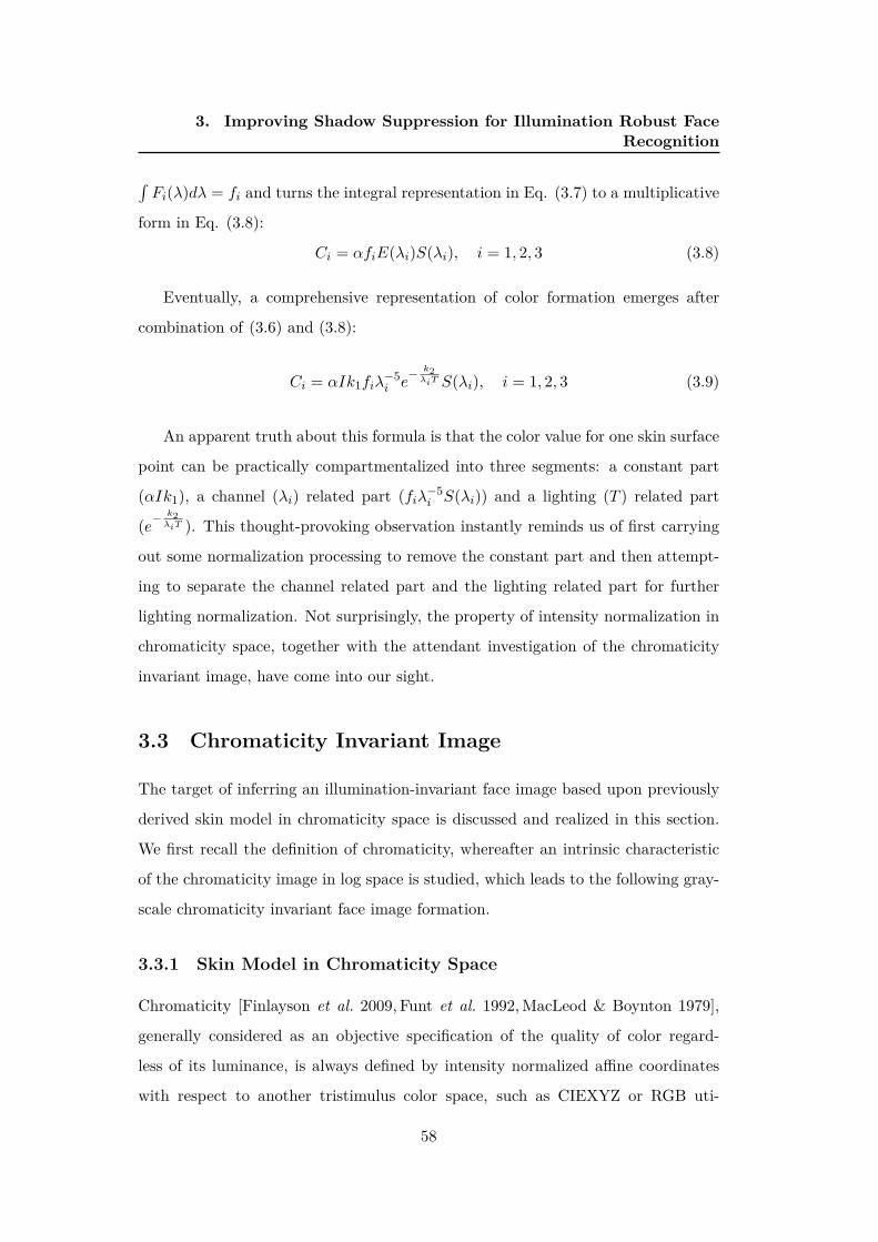
3. Improving Shadow Suppression for Illumination Robust FaceRecognition
∫Fi(λ)dλ = fi and turns the integral representation in Eq. (3.7) to a multiplicative
form in Eq. (3.8):
Ci = αfiE(λi)S(λi), i = 1, 2, 3 (3.8)
Eventually, a comprehensive representation of color formation emerges after
combination of (3.6) and (3.8):
Ci = αIk1fiλ−5i e
− k2λiT S(λi), i = 1, 2, 3 (3.9)
An apparent truth about this formula is that the color value for one skin surface
point can be practically compartmentalized into three segments: a constant part
(αIk1), a channel (λi) related part (fiλ−5i S(λi)) and a lighting (T ) related part
(e−k2λiT ). This thought-provoking observation instantly reminds us of first carrying
out some normalization processing to remove the constant part and then attempt-
ing to separate the channel related part and the lighting related part for further
lighting normalization. Not surprisingly, the property of intensity normalization in
chromaticity space, together with the attendant investigation of the chromaticity
invariant image, have come into our sight.
3.3 Chromaticity Invariant Image
The target of inferring an illumination-invariant face image based upon previously
derived skin model in chromaticity space is discussed and realized in this section.
We first recall the definition of chromaticity, whereafter an intrinsic characteristic
of the chromaticity image in log space is studied, which leads to the following gray-
scale chromaticity invariant face image formation.
3.3.1 Skin Model in Chromaticity Space
Chromaticity [Finlayson et al. 2009, Funt et al. 1992, MacLeod & Boynton 1979],
generally considered as an objective specification of the quality of color regard-
less of its luminance, is always defined by intensity normalized affine coordinates
with respect to another tristimulus color space, such as CIEXYZ or RGB uti-
58

3. Improving Shadow Suppression for Illumination Robust FaceRecognition
lized in our case. The normalization mapping mainly contains two modalities:
L1-normalization: c = r, g, b = R,G,B/(R + G + B) or geometric mean nor-
malization: c = r, g, b = R,G,B/ 3√R ∗G ∗B, in both normalization methods,
all colors are regularized to equiluminous ones in this space which helps to attenuate
the effect of the intensity component.
For computational efficiency and further extension, the geometric-mean-
normalized chromaticity is implemented as a processing pipeline for skin color in
Eq. (3.9). The c = r, g, b values in chromaticity space are given as follows:
ci =fiλ
−5i S(λi)
(3∏
j=1fjλ
−5j S(λj))
13
e− k2
λiT
e
13
3∑j=1
− k2λjT
, i = 1, 2, 3 (3.10)
Within this chromaticity representation, all constant terms are normalized. The
remaining two terms consist of a channel-related one and a lighting-related one. If
we switch our focus back to the process of highlight detection in the previous section
which aims at separating specular reflection from diffuse reflection, the explanation
could be sufficiently given: only under the assumption of the Lambertian model can
we be capable of normalizing the constant terms benefiting from the multiplicative
representation of skin color.
So far, we solidify and parametrize an exhaustive color formation model in a
concise form. More specifically, this representation could be naturally considered as
an aggregation of a lighting-invariant part and another lighting-related part, which
grants us the opportunity to further explore the illumination invariant components.
3.3.2 Chromaticity Invariant Image Generation
When investigating the characteristics of the skin model in chromaticity space, both
its multiplicative form and the exponential terms easily guide us to the logarithm
processing, which is capable of transforming Eq. (3.10) to:
ψi = log(ci) = log Wi
W+ (−k2
λi− 1
3
3∑j=1
−k2λj
)/T, (3.11)
59

3. Improving Shadow Suppression for Illumination Robust FaceRecognition
with the lighting-invariant components Wi = fiλ−5i S(λi) and W =
(3∏
j=1fiλ
−5j S(λj))
13 .
It is noticeable that all three chromaticity color channels in log space are charac-
terized by the identical lighting color T which implies the potential linear correlation
among these values. Let’s consider another fact: c1 ∗ c2 ∗ c3 = 1 since they are geo-
metric mean normalized values, hence it could be equally inferred that in log space
we have ψ1+ψ2+ψ3 = 0, illustrating that all chromaticity points ψ = (ψ1, ψ2, ψ3)
in 3D log space actually fall onto a specific plane perpendicular to its unit normal
vector u = 1/√3(1, 1, 1).
Up to now, the dimensionality of target space has been reduced to 2. It becomes
reasonable to bring in a 3D-2D projection in order to make the geometric significance
more intuitive. Derived from the projector P⊥u = I−uTu = UTU onto this plane,
U = [u1;u2] is a 2 × 3 orthogonal matrix formed by two nonzero eigenvectors of
the projector which is able to transform the original 3D vector ψ to 2D coordinates
ϕ within this plane. This transformation process is portrayed in Eq. (3.12).
ϕ = UψT = [u1 · ψT ;u2 · ψT ], (3.12)
with u1 = [ 1√2,− 1√
2, 0],u2 = [ 1√
6, 1√
6,− 2√
6].
Along with the substitution of Eq. (3.11) in Eq. (3.12), we are able to derive
the 2D coordinates of chromaticity image pixels analytically as follows:
ϕ =
ϕ1ϕ2
=
√22 (d1 + (− k2
λ1+ k2
λ2)/T )
√66 (d2 + (− k2
λ1− k2
λ2+ 2k2
λ3)/T )
(3.13)
with d1 = log(W1W2
), d2 = log(W1W2
W 23
).
The property of linearity in the projected plane could be straightforwardly de-
duced through a further analysis of (3.13):
ϕ2 =
√3
3
λ1(λ2 − λ3) + λ2(λ1 − λ3)
(λ1 − λ2)λ3ϕ1 + d (3.14)
where d is an offset term determined by W1,W2,W3. Considering thatWi depends
60

3. Improving Shadow Suppression for Illumination Robust FaceRecognition
(a) (b)
(c) (d)
Figure 3.4: Linearity of chromaticity image pixels in log space. (a) Original image.(b) chromaticity pixel values in 3D log space. (c) Pixels of forehead area in projectedplane. (d) Pixels of nose bridge area in projected plane.
merely on object surface reflectance and remains constant for a given geometry even
under varying lighting conditions, the points projected onto this plane should take
the form of straight lines with the same slope. Moreover, points belonging to
the same material should be located on the same line and the length of each line
shows the variation range of lighting with respect to this material. Accordingly, the
distance between each pair of parallel lines reflects the difference between different
object surface properties behind them.
The above inference is evidenced and supported by illustrations in Fig. 3.4.
Firstly, Fig. 3.4b shows that all chromaticity image points fall onto the same plane
of which the normal vector, depicted with a fine blue line, is u = 1/√3(1, 1, 1);
then, we choose two sub-regions in the original image for the linearity study since
the whole image contains excessive points for demonstration. Fig. 3.4c and Fig.
3.4d respectively represent the projected 2D chromaticity pixels in forehead and
nose bridge rectangles where two approximately parallel line-shaped clusters can be
61

3. Improving Shadow Suppression for Illumination Robust FaceRecognition
obviously observed. In particular, the chosen nose bridge area bears more lighting
changes while there is only unchanged directional lighting in the forehead area for
comparative analysis. Correspondingly, the straight line in Fig. 3.4c holds a smaller
range than that in Fig. 3.4d.
3.3.3 Entropy based Lighting Normalization
Note that all 2D chromaticity image pixels are scattered into line-shaped clusters
differentiated by their corresponding surface attributes. To estimate the intrinsic
property of different materials in chromaticity images, we would like to further
reduce the dimensionality of chromaticity space.
According to [Barron & Malik 2015], global parsimony priors on reflectance
could hold as a soft constraint. Under this assumption, only a small number of
reflectances are expected in an object-specific image, and we reasonably extend this
assumption to our own work which implies that lighting normalization substantially
decreases the probability distribution of disorder in a human face image. Within this
pipeline, we seek for a projection direction, parametrized by angle θ, which should
be exactly perpendicular to the direction of straight lines formed on the projected
plane. Inasmuch as points of the same material across various illuminations fall
on the same straight line, the 2D-1D projection of them onto a line with angle θ
will result in an identical value which could be literally treated as an intrinsic value
of this material. During this 2D-1D projection formulated in (3.15), chromaticity
image is finally transformed to a 1D gray-scale image.
χ = ϕ1 cos θ + ϕ2 sin θ (3.15)
With this in mind, the most appropriate projection direction could be found
by minimizing the entropy of projected data. To begin with, we adopt Freedman-
Diaconis rule [Freedman & Diaconis 1981] for the purpose of deciding the bin width
as h = 2Q(χ)
n1/3 , here n refers to the number of projected points. Compared with the
commonly used Scott’s rule, Freedman-Diaconis rule replaces the standard deviation
of data by its interquartile range, denoted by Q(χ), which is therefore more robust
62
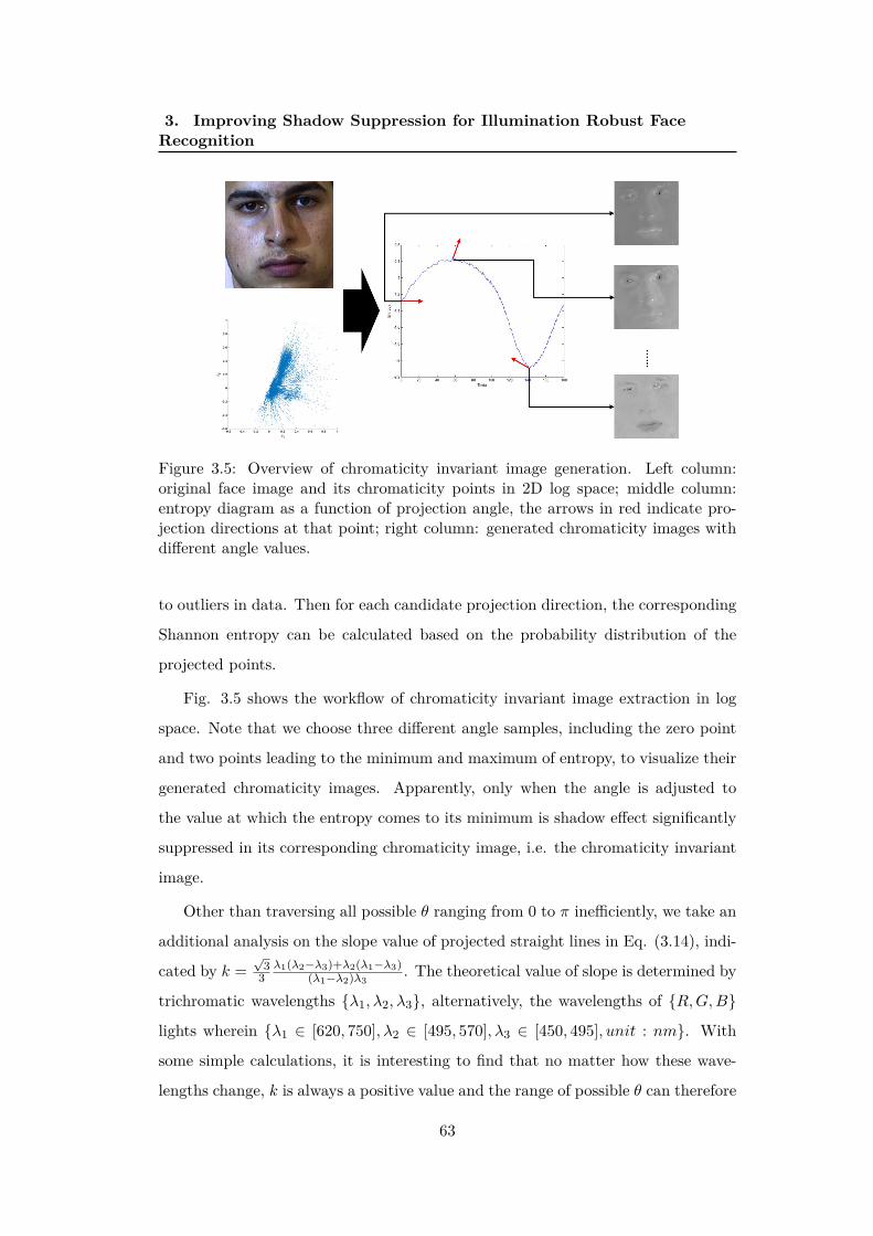
3. Improving Shadow Suppression for Illumination Robust FaceRecognition
Figure 3.5: Overview of chromaticity invariant image generation. Left column:original face image and its chromaticity points in 2D log space; middle column:entropy diagram as a function of projection angle, the arrows in red indicate pro-jection directions at that point; right column: generated chromaticity images withdifferent angle values.
to outliers in data. Then for each candidate projection direction, the corresponding
Shannon entropy can be calculated based on the probability distribution of the
projected points.
Fig. 3.5 shows the workflow of chromaticity invariant image extraction in log
space. Note that we choose three different angle samples, including the zero point
and two points leading to the minimum and maximum of entropy, to visualize their
generated chromaticity images. Apparently, only when the angle is adjusted to
the value at which the entropy comes to its minimum is shadow effect significantly
suppressed in its corresponding chromaticity image, i.e. the chromaticity invariant
image.
Other than traversing all possible θ ranging from 0 to π inefficiently, we take an
additional analysis on the slope value of projected straight lines in Eq. (3.14), indi-
cated by k =√33
λ1(λ2−λ3)+λ2(λ1−λ3)(λ1−λ2)λ3
. The theoretical value of slope is determined by
trichromatic wavelengths λ1, λ2, λ3, alternatively, the wavelengths of R,G,B
lights wherein λ1 ∈ [620, 750], λ2 ∈ [495, 570], λ3 ∈ [450, 495], unit : nm. With
some simple calculations, it is interesting to find that no matter how these wave-
lengths change, k is always a positive value and the range of possible θ can therefore
63

3. Improving Shadow Suppression for Illumination Robust FaceRecognition
be restricted to [π/2, π] which helps to greatly reduce the computational load.
3.3.4 Global Intensity Regularization
Notwithstanding the illumination normalization, projected shadow-free images may
suffer from global intensity differences across images caused by original lighting
conditions and by outliers. A final global regularization module is consequently
integrated in order to overcome this drawback. In this step, the most dominant
intensity of the resulting image is first approximated by a simple strategy:
µ = (mean(χ(x, y)m))m (3.16)
where m is a regularization coefficient which considerably decreases the impact of
large values. We take m = 0.1 by default following the setup in the work of Tan et
al. [Tan & Triggs 2010]. Next, this reference value is chosen to represent the color
intensity of most face skin area and is scaled to 0.5 in a double-precision gray-scale
image with data in the range [0,1]. The same scale ratio is then applied to all pixels
to gain the final image.
3.4 Shadow-free Color Face Recovery
Though the representation of the 1D chromaticity invariant image contains suc-
cessfully normalized lighting variations across the whole face image, it is flawed due
to the loss of textural details during the process of dimensionality reduction which
leads to low contrast images as depicted in Fig. 3.5. A full color image reconstruc-
tion module is therefore required to both improve the realism of generated images
and improve the performance of our method in face analysis.
3.4.1 In-depth Analysis of 1D Chromaticity Image
Given a chromaticity invariant image and all projection matrices, a general idea
to reconstruct its color version is to project reversely its 1D lighting-normalized
points to 2D/3D space in steps. However, this solution is virtually impracticable
64

3. Improving Shadow Suppression for Illumination Robust FaceRecognition
due to two facts: 1) the recovery of overall intensity in each color band is an ill-
posed problem since the shadow removal method is designed only for chromaticity
values, 2) considerable textural features, such as the mustache and the eyebrow,
are undesirably eliminated or wrongly recognized as being skin during the forward
2D/1D projection. Thus an extra analysis on representation of RGB channels in
log space is conducted.
Derived from equation Eq. (3.9), the logarithmic representation of RGB values,
denoted by Li, could be written as a two-component addition:
Li = log(αIk1fiλ−5i S(λi))−
k2λiT
, i = 1, 2, 3 (3.17)
It is worth noting that the first additive component in the above equation
consists of spatially varying factors while the second additive term is lighting-
dependent. Given an illumination-invariant region, the gradients at pixel (x,y)
are then computed during inference:
∇xLi(x, y, T ) =Li(x+∆x, y, T )− Li(x, y, T )
∆x
∇yLi(x, y, T ) =Li(x, y +∆y, T )− Li(x, y, T )
∆y
(3.18)
Based on evidence in [Finlayson et al. 2006] and [Land & McCann 1971], lighting
conditions change slowly across a face image except for shadow edges. Consequently,
for the partial derivative of the log-image with respect to x at any pixel (x, y) which
appears out of shadow edges we have:
∇xLi(x, y, T1) = ∇xLi(x, y, T2), ∀(T1, T2) (3.19)
where T1 and T2 refer to different lighting conditions such as illuminated part and
shadow part and this property holds equally for the partial derivative with respect
to y.
To summarize, lighting conditions across a log-image are mainly changed on the
boundary of shadow area, i.e. for any pixel inside or outside this boundary, the
spatial gradient is practically lighting-invariant. Motivated by this, we will derive
65

3. Improving Shadow Suppression for Illumination Robust FaceRecognition
a shadow-specific edge detection method analytically.
3.4.2 Shadow-Specific Edge Detection
The ability to separate out shadow-specific edges from edges between different fa-
cial parts is crucial. To achieve this aim, we trace back the generation of the 1D
chromaticity invariant image, where the shadow edges are removed by an orthog-
onal projection. Note that this projection was determined by an angle θmin which
minimizes the entropy of Eq. (3.15). Conversely, a ’wrong’ projection angle would
retain or even highlight the shadow edge.
More specifically, we seek a novel direction θmax along which the projection
of chromaticity pixels to 1D tends to clearly preserve the chaos caused by vary-
ing lighting conditions. The θmax could be estimated by maximizing the entropy.
Theoretically, the freshly projected 1D image contains edges caused by both fa-
cial features and lighting variations, thus would be considered to be different from
the chromaticity invariant image in order to obtain the shadow-specific edge mask
M(x, y).
Furthermore, considering that lighting effects could be specially enhanced in one
of the two dimensions described in Eq. (3.13), we define M(x, y) as follows while
combining comparisons in both re-projected ϕmin1 , ϕmin
2 and ϕmax1 , ϕmax
2 :
M(x, y) =
1 if ∥ϕ′min∥ < τ1 & ∥ϕ′
max∥ > τ2
0 otherwise(3.20)
where ∥ϕ′min∥ = max(∥∇ϕmin
1 ∥, ∥∇ϕmin2 ∥), ∥ϕ′
max∥ = max(∥∇ϕmax1 ∥, ∥∇ϕmax
2 ∥)
and τ1, τ2 are two pre-defined thresholds.
It is worth mentioning that all 2D chromaticity images derived from both θmax
and θmin are preprocessed by guided filter [He et al. 2010] to facilitate the gradient
calculation on a smoother version. As regards the choice of guided filter, we use
matrix of ones for the chromaticity invariant image to average the intensity. Con-
versely, the chromaticity image with shadows will take itself for guided filtering to
enforce the gradient map.
66
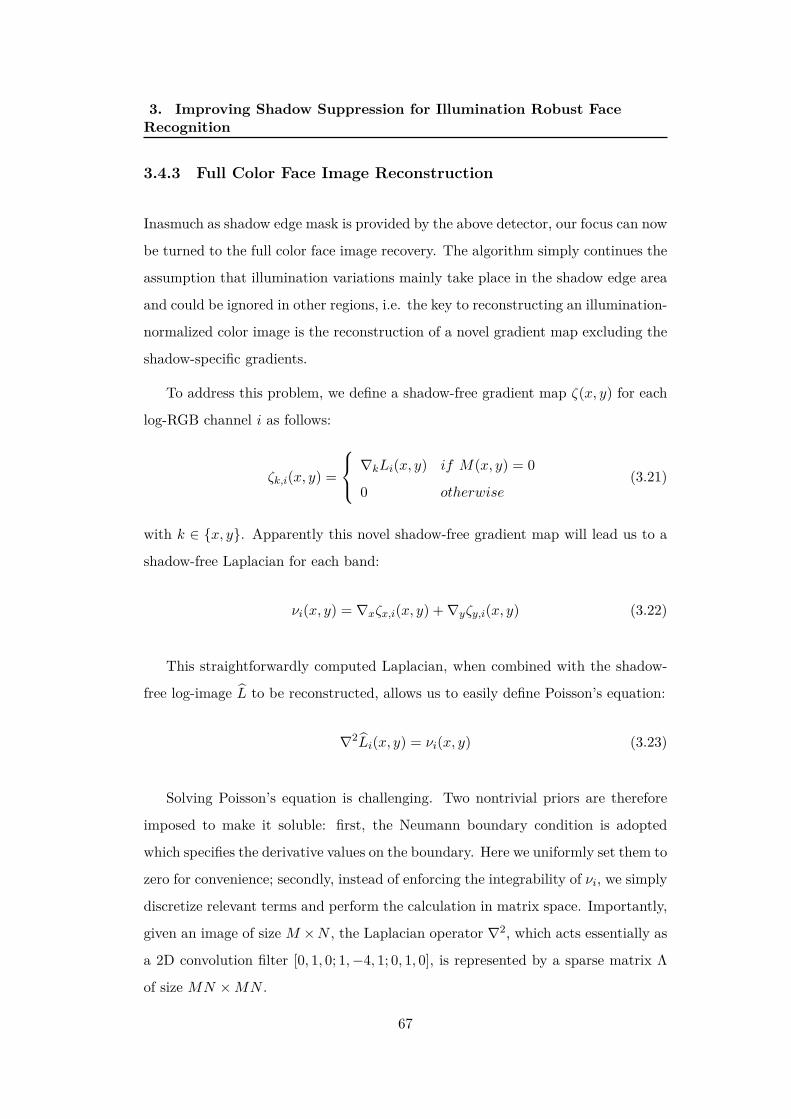
3. Improving Shadow Suppression for Illumination Robust FaceRecognition
3.4.3 Full Color Face Image Reconstruction
Inasmuch as shadow edge mask is provided by the above detector, our focus can now
be turned to the full color face image recovery. The algorithm simply continues the
assumption that illumination variations mainly take place in the shadow edge area
and could be ignored in other regions, i.e. the key to reconstructing an illumination-
normalized color image is the reconstruction of a novel gradient map excluding the
shadow-specific gradients.
To address this problem, we define a shadow-free gradient map ζ(x, y) for each
log-RGB channel i as follows:
ζk,i(x, y) =
∇kLi(x, y) if M(x, y) = 0
0 otherwise(3.21)
with k ∈ x, y. Apparently this novel shadow-free gradient map will lead us to a
shadow-free Laplacian for each band:
νi(x, y) = ∇xζx,i(x, y) +∇yζy,i(x, y) (3.22)
This straightforwardly computed Laplacian, when combined with the shadow-
free log-image L to be reconstructed, allows us to easily define Poisson’s equation:
∇2Li(x, y) = νi(x, y) (3.23)
Solving Poisson’s equation is challenging. Two nontrivial priors are therefore
imposed to make it soluble: first, the Neumann boundary condition is adopted
which specifies the derivative values on the boundary. Here we uniformly set them to
zero for convenience; secondly, instead of enforcing the integrability of νi, we simply
discretize relevant terms and perform the calculation in matrix space. Importantly,
given an image of size M ×N , the Laplacian operator ∇2, which acts essentially as
a 2D convolution filter [0, 1, 0; 1,−4, 1; 0, 1, 0], is represented by a sparse matrix Λ
of size MN ×MN .
67

3. Improving Shadow Suppression for Illumination Robust FaceRecognition
Let
D =
−4 1 0 0 0 · · · 0
1 −4 1 0 0 · · · 0
0 1 −4 1 0 · · · 0...
......
...... . . . ...
0 · · · 0 1 −4 1 0
0 · · · 0 0 1 −4 1
0 · · · 0 0 0 1 −4
(3.24)
and I denotes an M ×M unit matrix. We have
Λ =
D I 0 0 0 · · · 0
I D I 0 0 · · · 0
0 I D I 0 · · · 0...
......
...... . . . ...
0 · · · 0 I D I 0
0 · · · 0 0 I D I
0 · · · 0 0 0 I D
(3.25)
Each row of Λ corresponds to a sparse full-size filter for one pixel, and Li could
be accordingly solved by a left division:
Li = Λ \ νi (3.26)
After exponentiating Li, a multiplicative scale factor per channel, which is com-
puted by retaining the intensity of brightest pixels in raw image, will be finally
applied to ensure that not only color but also intensity information is properly re-
covered. See Fig. 3.6 for a demonstration of shadow-specific edge detection and
color face recovery results.
68

3. Improving Shadow Suppression for Illumination Robust FaceRecognition
Figure 3.6: Overview of edge mask detection and full color face recovery. (a) and(f) are raw and recovered face image; (b), (c) and (d) depict respectively 1D/2Dchromaticity images and edge maps, note that in each figure the upper row refersto shadow-free version and the lower row is shadow-retained version; (e) is the finaldetected edge mask.
3.5 Experimental Results
To quantitatively evaluate the universality and robustness of the proposed method,
experiments for face recognition were carried out on several publicly available face
databases, which incorporate a great deal of variety in terms of illumination envi-
ronments. For each database, we adopt the standard evaluation protocols reported
in the face analysis literature and present how the proposed approach improves FR
performance.
3.5.1 Databases and Experimental Settings
Databases. In light of the fact that our method aims to normalize and recover
illumination in RGB color space, two criteria need to be fulfilled in selecting a
database: that it includes face images taken with various lighting conditions; and
that all images are provided with full color information. The two selected databases
are as follows:
69

3. Improving Shadow Suppression for Illumination Robust FaceRecognition
• The CMU-PIE database [Sim et al. 2003] has been very influential and
prevalent in robust face recognition across pose, illumination and expression
variations. It contains 41368 images from 68 identities, including 13 different
poses, 43 different illumination conditions and 4 expressions. Here we restrict
our attention merely to geometrically aligned frontal face views with neutral
expression across illumination variations, wherein the experimental protocol
in [Han et al. 2013] is adopted.
• The Face Recognition Grand Challenge (FRGC) ver2.0 database [Phillips
et al. 2005] is a well-known face database designed for multitask 2D/3D FR
evaluations. There are 12,776 still images and 943 3D scans from 222 identities
in the training set. Accordingly, 4,007 3D scans and more than 22,000 images
from 466 identities are stored in the validation set. Specifically, this database
contains various scale and image resolutions as well as expression, lighting and
pose variations. The standard protocol of Exp.4 defined in [Phillips et al. 2005]
targeting at lighting relevant tasks is used in our FR experiments.
For the first subject of each database, Fig. 3.7 gives an illustration of some im-
age samples across varying illumination environments. Note that all facial images
are cropped and the resolution is 180×180. As can be visualized from these figures,
CMU-PIE database contains well-controlled illuminations and strictly unchanged
pose for one subject while FRGC database contributes more to the variations on
illumination and pose, which makes our evaluation process comprehensive and reli-
able.
Table 3.1 gives detailed structure as well as experimental protocol for each
database. According to commonly used protocols, two different tasks are pro-
posed for these two databases: 1-v-n face identification for CMU-PIE and 1-v-1
face verification for FRGC, which will be further detailed in upcoming subsections.
Features. To evaluate performance robustness under different feature extraction
algorithms, we have experimented with four popular descriptors in face recognition,
including Local Binary Pattern (LBP), Local Phase Quantization (LPQ), Local
Gabor Binary Pattern (LGBP) and deep CNN based face descriptor (VGG-Face),
70

3. Improving Shadow Suppression for Illumination Robust FaceRecognition
(a)
(b)
Figure 3.7: Cropped face examples of the first subject in the (a): CMU-PIEdatabase; (b): FRGC database.
Table 3.1: Overview of database division in our experiments
Database PersonTarget Set Query Set
Lighting Images Lighting Images
CMU-PIE 68 3 204 18 1,224FRGC 466 controlled 16,028 uncontrolled 8,014
71

3. Improving Shadow Suppression for Illumination Robust FaceRecognition
the parameter settings for each of them are detailed as follows:
• LBP [Ahonen et al. 2006]: For each face image a 59-dimensional uniform LBP
histogram feature is extracted. For the LBP computation we set the number of
sample points as 8 and radius as 2. Chi-square distance is computed between
two LBP histogram features to represent their dissimilarity.
• LPQ [Ahonen et al. 2008]: We set size of the local uniform window as 5
and the correlation coefficient ρ as 0.9. Accordingly, the α for the short-time
Fourier transform equals the reciprocal of window size, i.e. α = 0.2. With
the process of decorrelation, the output feature for each image is a 256D
normalized histogram of LPQ codewords and Chi-square distance is applied
as well in our experiments as a matching criterion.
• LGBP [Zhang et al. 2005b]: For each face image, 4 wavelet scales and 6 filter
orientations are considered to generate 24 Gabor kernels. Similarly to LBP,
holistic LGBP features are extracted for test images, resulting in 1,416D fea-
ture vectors. A simple histogram-intersection-matching described in [Zhang
et al. 2005b] is used as similarity measurement.
• VGG-Face [Parkhi et al. 2015a]: The VGG-Face descriptors are computed
based on the VGG-Very-Deep-16 CNN architecture in [Parkhi et al. 2015a]
which achieves state-of-the-art performance on all popular FR benchmarks.
Here we simply take the well learned model provided by the authors and
replace the last Softmax layer by identity module in order to extract 4,096D
features for test images.
Methods. The main contributions of our method are to remove shadows and
recover illumination-normalized color face images instead of de-lighting in gray-scale
like all other existing methods do. To better present the effectiveness and necessity
of the proposed method, we implement it as a preprocessing followed by other
gray-scale level lighting normalization techniques to test the fusion performance
compared with the results obtained without using our method. As an exception to
the above, for VGG-Face model which requires RGB images as input, we conduct
72

3. Improving Shadow Suppression for Illumination Robust FaceRecognition
the comparison only between original images and shadow-free recovered images with
no gray-scale level lighting normalization.
For this comparative study, a bunch of gray-scale space based approaches are in-
cluded, including basic methods such as Gaussian filter based normalization (DOG),
Gradient faces based normalization (GRF) [Zhang et al. 2009b], wavelet based
normalization (WA) [Du & Ward 2005], wavelet-based denoising (WD) [Zhang
et al. 2009a], single-scale and multi-scale retinex algorithms (SSR and MSR) [Job-
son et al. 1997a,Jobson et al. 1997b], and state-of-art methods such as logarithmic
discrete cosine transform (DCT) [Chen et al. 2006b], single-scale and multi-scale
self-quotient image (SQI and MSQ) [Wang et al. 2004], single-scale and multi-scale
Weberfaces normalization (WEB and MSW) [Wang et al. 2011], additionally, a well-
known fusing preprocessing chain (TT) [Tan & Triggs 2010] is also experimented.
Thankfully, an off-the-shelf implementation provided by Štruc and Pavešić [Štruc
& Pavešic 2011, Štruc & Pavešić 2009], namely INface Toolbox, grants us the op-
portunity to achieve our target efficiently and accurately.
3.5.2 Visual Comparison and Discussion
Shadows. First , a comparison of shadow removal results on soft and hard shadows
is conducted and depicted in Fig. 3.8. We can make two observations from these
results:
1. From a holistic viewpoint, our proposed method handles well the removal of
both hard and soft edge shadows. In both cases, the lighting intensity across
the whole image is normalized and the effects of shadows are eliminated.
2. Specified in dashed-red and dashed-blue rectangles respectively, the two mid-
dle image patches show us the differences while processing different shadows.
Despite visually similar results, for face images on the left with a hard-edged
shadow, shadow removal performance is actually more robust than for the im-
age on the right with soft shadows because more facial details are smoothed
for soft shadows where shadow edges are difficult to define. This drawback
may also affect the performance of face recognition which will be detailed in
73
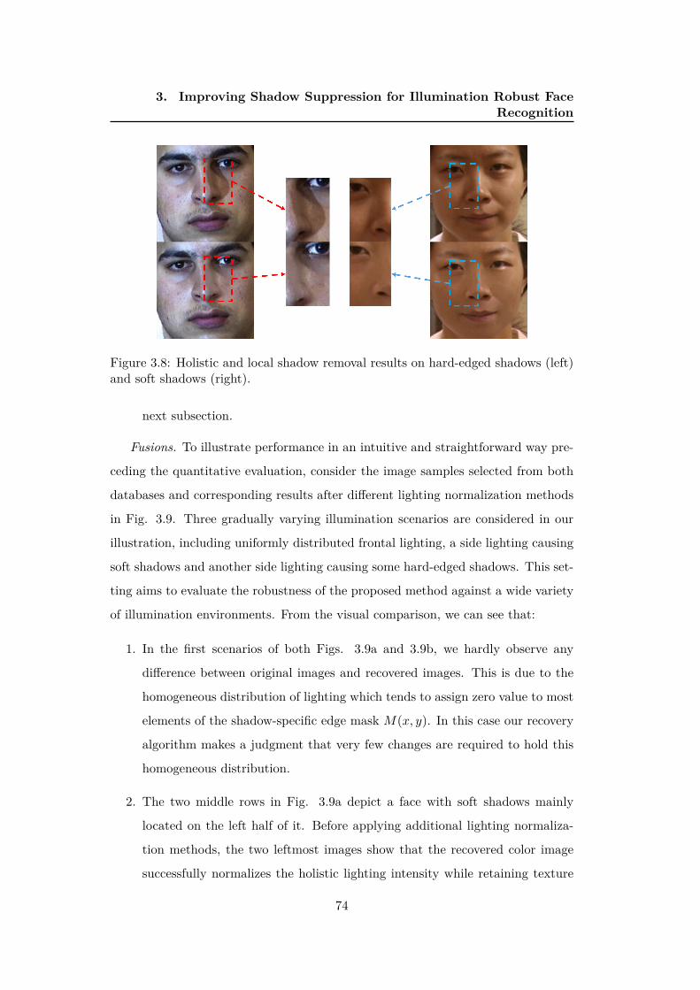
3. Improving Shadow Suppression for Illumination Robust FaceRecognition
Figure 3.8: Holistic and local shadow removal results on hard-edged shadows (left)and soft shadows (right).
next subsection.
Fusions. To illustrate performance in an intuitive and straightforward way pre-
ceding the quantitative evaluation, consider the image samples selected from both
databases and corresponding results after different lighting normalization methods
in Fig. 3.9. Three gradually varying illumination scenarios are considered in our
illustration, including uniformly distributed frontal lighting, a side lighting causing
soft shadows and another side lighting causing some hard-edged shadows. This set-
ting aims to evaluate the robustness of the proposed method against a wide variety
of illumination environments. From the visual comparison, we can see that:
1. In the first scenarios of both Figs. 3.9a and 3.9b, we hardly observe any
difference between original images and recovered images. This is due to the
homogeneous distribution of lighting which tends to assign zero value to most
elements of the shadow-specific edge mask M(x, y). In this case our recovery
algorithm makes a judgment that very few changes are required to hold this
homogeneous distribution.
2. The two middle rows in Fig. 3.9a depict a face with soft shadows mainly
located on the left half of it. Before applying additional lighting normaliza-
tion methods, the two leftmost images show that the recovered color image
successfully normalizes the holistic lighting intensity while retaining texture
74

3. Improving Shadow Suppression for Illumination Robust FaceRecognition
(a)
(b)
Figure 3.9: Illustration of illumination normalization performance of two samples in(a) CMU-PIE and (b) FRGC database. For each sample, three lighting conditionsare considered, from top to bottom are the image with frontal lighting, image withsoft shadows and image with hard-edged shadows.The columns represent differentlighting normalization techniques to be fused with original color image or CII recov-ered color image. Green framed box: a comparison sample pair with soft shadows.Red framed box: a comparison sample pair with hard-edged shadows.
75

3. Improving Shadow Suppression for Illumination Robust FaceRecognition
details on the left half of the face. This property can also be evidenced by
contrast after fusion with a diverse range of lighting normalization methods.
Note that most of these techniques could handle perfectly the removal of soft
shadows such as DCT, SQI, SSR and TT. For these techniques visually in-
distinguishable results are obtained on both original images and recovered
images. On the other hand, for techniques which are less robust to soft shad-
ows such as WA (visualized in green boxes), taking the recovered image as
input enables a globally normalized lighting intensity where dark regions, es-
pecially the area around eyes, are brightened. Compared with the original
image, this process gives a better visualization result. Different from the first
subject in CMU-PIE, we choose a female face from FRGC with a more compli-
cated illumination condition where shadows are more scattered, even though
certain shadows still remain around mouth with the proposed method. we can
nevertheless perceive the improvement of shadow suppression on the upper
half of the face.
3. The two bottom rows in Fig. 3.9a and 3.9b focus on hard-edged shadows
caused by occlusion by the nose and glasses against the lighting direction,
respectively. Under this scenario, resulting images generated by adopting
the proposed recovery method as preprocessing show distinct advantages over
those generated from the original image. This kind of shadow edge is difficult
to remove for existing lighting normalization methods, including the state-of-
art algorithm TT (visualized in red boxes), because these methods can hardly
distinguish shadow edges from the intrinsic facial texture.
To summarize, according to the results of visual comparison, our shadow-free
color face image recovery algorithm could (1) provide intuitively identical results
to original images when illumination is homogeneously distributed everywhere; (2)
normalize holistic lighting in color space when soft shadows occur and could be
further fused with other methods in gray scale space; (3) be performed as a supple-
mentary measure specifically to remove hard-edged shadows before applying other
lighting normalization approaches.
76

3. Improving Shadow Suppression for Illumination Robust FaceRecognition
Figure 3.10: Faces in the wild before (top) and after (bottom) shadow removal.From left to right we choose images with a gradual decrease (left: strong, middletwo: moderate, right: weak) in shadow intensity.
Faces in the wild. To further analyze the effectiveness and limitation of
our approach, we conduct additional experiments on natural face images in the
wild with a far wider range of lighting conditions. The first row of Fig. 3.10
illustrates four face images with a gradual decrease in shadow intensity. As can be
seen on the bottom row images after shadow removal, our method can effectively
handle faces under moderate lighting conditions (middle two images) quite well.
However, it will fail when holistic lighting is poor with intense shadows (first image),
or when holistic lighting is too bright with soft shadows (last image). In both
cases, lighting conditions are saturated (pixel values are limited by either 0 or 255)
and, accordingly, our assumption of linearity in chromaticity space becomes much
weaker.
3.5.3 Identification Results on CMU-PIE
A rank-1 face identification task is generally described as a 1-to-n matching system,
where n refers to the number of recordings in the target set, which aims to find a
single identity in the target set best fitting the query face image through similarity
measurement. In this scenario, closed-set identification is performed on various
77

3. Improving Shadow Suppression for Illumination Robust FaceRecognition
recognition algorithms to evaluate the robustness of our method.
Table 3.2 tabulates the identification rate for different features. For each feature
and each gray-scale lighting normalization method, we compare the results before
and after taking the CII recovery algorithm as preprocessing. The higher accuracy
is highlighted for each comparison pair. Several observations could be made from
these results:
1. Generally, fusing our proposed method in the preprocessing chain helps im-
prove performance on this identification task with different gray-scale lighting
normalization approaches and different features. This is because our method
emphasizes the removal of shadow edges while all other methods suffer from
retaining such unwanted extrinsic features.
2. Without other gray-scale methods (N/A in the Table) or even with gray-scale
methods such as WA which are relatively less robust to lighting variations,
the results based on the CII recovered color image significantly boost the
performance compared with using other methods. This observation implies
that besides the effect of shadow edge removal, our method also provides us
with holistic lighting normalization as well.
3. For some gray-scale methods like SQI and MSQ, our method causes slight yet
unpleasant side effects with LBP and LPQ features. This is probably due to
the phenomenon previously observed in visual comparison that the proposed
method will smooth the region detected as shadow edges, SQI and MSQ may
become more sensitive to this unrealistic smoothness because images would be
further divided by their smoothed version. Nevertheless, with LGBP features
the proposed method still achieves better results with SQI and MSQ because
the introduction of 24 Gabor filters helps alleviate the effect of the smoothed
region.
4. The fusion of our method and TT failed to gain performance improvement. As
a preprocessing sequence itself, TT has been carefully adjusted to the utmost
extent so it is difficult to combine it with other preprocessing.
78

3. Improving Shadow Suppression for Illumination Robust FaceRecognition
Tabl
e3.
2:R
ank-
1R
ecog
nitio
nR
ates
(Per
cent
)of
Diff
eren
tM
etho
dson
CM
U-P
IED
atab
ase
Feat
ure
Prep
roce
ssin
gG
ray-
Scal
eLi
ghtin
gN
orm
aliz
atio
nM
etho
ds
N/A
GR
FW
DW
AD
CT
DO
GW
EBM
SWSQ
IM
SQSS
RM
SRT
T
LBP
Orig
inal
44.0
32.8
20.8
39.2
72.6
65.4
59.2
58.9
61.4
71.8
66.8
67.7
67.7
CII
Rec
over
y48
.334
.123
.045
.675
.366
.059
.861
.061
.370
.968
.869
.865
.6
LPQ
Orig
inal
58.0
34.7
37.9
49.6
85.2
79.1
73.9
77.6
74.0
80.2
84.4
84.8
82.4
CII
Rec
over
y62
.635
.135
.555
.386
.681
.075
.775
.173
.177
.188
.387
.482
.3
LGBP
Orig
inal
75.5
67.8
84.6
67.2
97.4
91.3
99.0
99.4
99.5
99.2
98.0
97.8
97.9
CII
Rec
over
y77
.674
.684
.872
.198
.093
.699
.499
.799
.699
.499
.598
.496
.7
VG
G-F
ace
Orig
inal
99.7
--
--
--
--
--
--
CII
Rec
over
y10
0-
--
--
--
--
--
-
79

3. Improving Shadow Suppression for Illumination Robust FaceRecognition
5. The VGG-Face model largely outperforms the other conventional features,
showing its impressive capacity in discriminative feature extraction and its
robustness against holistic lighting variations. Even in this case, the imple-
mentation of the proposed method is able to further perfect the performance
by dealing with the cast shadows.
3.5.4 Verification Results on FRGC
Notwithstanding its one-to-one characteristic, face verification in the FRGC
database is always considered as a much more challenging task when compared
with face identification on CMU-PIE. This is due to the fact that a large number
of face images in FRGC are captured in uncontrolled thus complicated illumination
environments with sensor or photon noise as well. For each preprocessing combina-
tion and each feature, we conduct a 16,028 × 8,014 pair matching and then compute
the verification rate based on this similarity/distance matrix. The experimental re-
sults are evaluated by Receiving Operator Characteristics (ROC), which represents
the Verification Rate (VR) varying with False Acceptance Rate (FAR).
Similarly to the previous experimental setting, we list the performance of dif-
ferent methods on the ROC value for FAR at 0.1% in Table 3.3. Moreover, corre-
sponding ROC curves for each gray-scale method are illustrated in Fig. 3.11. We
make our observations from these results:
1. Using the recovered color image is generally an effective way to improve the
performance on this verification task with different gray-scale methods and
features. Compared with the identification task on CMU-PIE, this effective-
ness is enhanced here since our method helps improve the verification rate at
FAR = 0.1% for almost all gray-scale methods with different features, vali-
dating the superiority of the proposed method.
2. A similar fact as in CMU-PIE is encountered again: the VGG-Face model can
greatly increase performance when compared with the other features, while
adding the proposed shadow removal preprocessing leads to a relatively slight
(1.1%) yet important improvement on this deep CNN model.
80

3. Improving Shadow Suppression for Illumination Robust FaceRecognition
Tabl
e3.
3:Ve
rifica
tion
Rat
e(P
erce
nt)
atFA
R=
0.1%
Usin
gD
iffer
ent
Met
hods
onFR
GC
V2.
0Ex
p.4
Feat
ure
Prep
roce
ssin
gG
ray-
Scal
eLi
ghtin
gN
orm
aliz
atio
nM
etho
ds
N/A
GR
FW
DW
AD
CT
DO
GW
EBM
SWSQ
IM
SQSS
RM
SRT
T
LBP
Orig
inal
1.0
12.8
3.5
1.1
6.0
14.5
18.5
17.7
18.5
12.3
3.8
3.9
15.7
CII
Rec
over
y1.
314
.85.
31.
56.
218
.823
.323
.125
.618
.05.
35.
920
.4
LPQ
Orig
inal
1.4
14.2
7.4
2.0
6.6
15.3
18.3
18.8
13.4
12.0
6.2
7.5
21.4
CII
Rec
over
y2.
017
.67.
52.
56.
714
.919
.119
.716
.815
.27.
38.
120
.2
LGBP
Orig
inal
13.0
31.0
18.8
12.7
28.2
37.0
37.9
35.7
29.1
30.9
27.2
28.2
38.8
CII
Rec
over
y16
.733
.225
.914
.329
.642
.438
.437
.031
.033
.129
.429
.944
.4
VG
G-F
ace
Orig
inal
92.5
--
--
--
--
--
--
CII
Rec
over
y93
.6-
--
--
--
--
--
-
81

3. Improving Shadow Suppression for Illumination Robust FaceRecognition
(a) (b) (c)
(d) (e) (f)
Figure 3.11: Several ROC curves for different gray-scale methods. (a) No gray-scalemethod, (b) GRF, (c) DOG, (d) WEB, (e) SQI, (f) TT. Note that only (a) containsROC curves for VGG-Face model because it requires RGB images as model input.
82
3. Improving Shadow Suppression for Illumination Robust FaceRecognition
3. The performance variance for different gray-scale methods is not totally con-
sistent with our previous observation on the CMU-PIE database. Unlike be-
fore, GRF, DOG and WEB achieve better results than DCT and SSR, which
implies that these methods are more robust while dealing with uncontrolled
and arbitrary lighting conditions.
3.6 Conclusion
In this chapter, we have presented a novel pipeline in chromaticity space for improv-
ing the performance on illumination-normalized face analysis. Our main contribu-
tions consist of: (1) introducing the concept of chromaticity space in face recognition
as a remedy to illumination variations, (2) achieving an intrinsic face image extrac-
tion processing and (3) realizing a photo-realistic full color face reconstruction after
shadow removal. Overall, the proposed approach explores physical interpretations
for skin color formation and is proven to be effective by improving performance for
FR across illumination variations on different databases. Meanwhile, it shows a
promising potential in practical applications for its photo-realism and extensibility.
Further efforts in developing this work will include synthesizing face images under
different illumination conditions and combining pose invariant techniques in order
to address face analysis problems in the wild.
83

4
Improving 2D-2.5D
Heterogeneous Face
Recognition with Conditional
Adversarial Networks
Contents
4.1 Introduction . . . . . . . . . . . . . . . . . . . . . . . . . . . . . 86
4.2 Baseline Cross-encoder Model . . . . . . . . . . . . . . . . . . 88
4.2.1 Background on Autoencoder . . . . . . . . . . . . . . . . . . 89
4.2.2 Discriminative Cross-Encoder . . . . . . . . . . . . . . . . . . 91
4.2.3 Multi-Criterion Mechanism . . . . . . . . . . . . . . . . . . . 94
4.2.4 Heterogeneous Face Recognition . . . . . . . . . . . . . . . . 96
4.3 CGAN based HFR Framework . . . . . . . . . . . . . . . . . . 96
4.3.1 Background on CGAN . . . . . . . . . . . . . . . . . . . . . . 97
4.3.2 CGAN Architecture . . . . . . . . . . . . . . . . . . . . . . . 99
4.3.3 Heterogeneous Face Recognition . . . . . . . . . . . . . . . . 101
4.4 Experimental Results . . . . . . . . . . . . . . . . . . . . . . . . 104
4.4.1 Dataset Collection . . . . . . . . . . . . . . . . . . . . . . . . 104
4.4.2 Implementation details . . . . . . . . . . . . . . . . . . . . . . 107
4.4.3 Reconstruction Results . . . . . . . . . . . . . . . . . . . . . . 108
4.4.4 2D-3D Asymmetric FR . . . . . . . . . . . . . . . . . . . . . 110
4.5 Conclusion . . . . . . . . . . . . . . . . . . . . . . . . . . . . . . 113

4. Improving 2D-2.5D Heterogeneous Face Recognition withConditional Adversarial Networks
4.1 Introduction
For decades, face recognition (FR) from color images has achieved substantial
progress and forms part of an ever-growing number of real world applications, such
as video surveillance, people tagging and virtual/augmented reality systems [Zhao
et al. 2003,Stan & Anil 2005,Tan et al. 2006,Abate et al. 2007,Azeem et al. 2014].
With the increasing demand for recognition accuracy under unconstrained condi-
tions, the weak points of 2D based FR methods become apparent: as an imaging-
based representation, color image is quite sensitive to numerous external factors,
such as lighting variations and makeup patterns. Therefore, 3D based FR tech-
niques [Scheenstra et al. 2005, Bowyer et al. 2006, Abate et al. 2007, Ding &
Tao 2016,Corneanu et al. 2016] have recently emerged as a remedy because they take
into consideration the intrinsic shape information of faces which is more robust while
dealing with these nuisance factors. Moreover, the complementary strengths of color
and depth data allow them to jointly work and gain further improvement [Husken
et al. 2005,Chang et al. 2005,Bowyer et al. 2006,Mian et al. 2007,Zhou et al. 2014].
Note that some 3D based techniques take the complete 3D face models as the shape
information while the other methods merely adopt range images (i.e. 2.5D images)
to provide depth values. The 3D models are advantageous in dealing with pose
variations, yet encounter problems with landmark localization and computational
cost. As a comparison, the 2.5D based methods can achieve state-of-the-art per-
formance with low cost on nearly frontal faces, furthermore, they can be combined
with other image-based techniques to enhance the flexibility.
However, 3D data is not always accessible in real-life conditions due to its special
requirements for optical instruments and acquisition environment. Likewise, other
challenges remain as well, including the real-time registration and preprocessing for
3D faces. An important question then naturally arises: can we design a recognition
pipeline where 3D faces are only registered in gallery while still providing signifi-
86

4. Improving 2D-2.5D Heterogeneous Face Recognition withConditional Adversarial Networks
cant information for the identification of unseen color images? To cope with this
problem, 2D-3D heterogeneous face recognition (HFR) [Toderici et al. 2010,Huang
et al. 2012,Zhao et al. 2013,Jin et al. 2014,Kakadiaris et al. 2016] has been proposed
as a reasonable workaround. As a worthwhile trade-off between purely 2D and 3D
based method, HFR adopts both color and depth data for training and gallery set
while the online probe set will simply contains color images. Under this mechanism,
a HFR framework can take full advantage of both color and depth information at
the training stage to reveal the correlation between them. Once learned, this cross-
modal correlation makes it possible to conduct heterogeneous matching between
preloaded depth images in gallery and color images digitally captured in real time.
Among the numerous attempts which have been made to propose impressive asym-
metric 2D/3D FR algorithms, either common subspace learning based methods or
synthesis methods are exploited to conduct the heterogeneous matching. However,
most current work relies on linear and shallow mapping strategies (e.g. CCA) to
construct common subspaces, which can hardly meet the demand of more compli-
cated situations.
Motivated by the considerations described above, in our work we resort to one
of the most representative and frontier technology, the deep CNN for driving ad-
vances. Note that all difficulties, which hinder us from availing ourselves of depth
information in probe set, come from the acquisition and registration of 3D data.
Intuitively, these problems can be immediately solved if we can reconstruct depth
images from color images accurately and efficiently. Therefore, as a preliminary
step, we first learn a baseline encoder-decoder network, namely Cross-encoder, for
depth estimation. This network takes a 2D image as input and the corresponding
2.5D as the reconstruction objective. The reconstructed 2.5D enables a straight-
forward 2.5D/2.5D comparison in the evaluation stage, meanwhile a discriminative
objective function is integrated which aims to generate an intermediate feature out-
put for 2D/2D FR. The dual FR phases would be ultimately combined to compute
a fusion score between gallery and probe.
Beyond the above synthesis-based mechanism, we take a further look at the
possibility of combining synthesis method and common subspace learning method.
87

4. Improving 2D-2.5D Heterogeneous Face Recognition withConditional Adversarial Networks
Thanks to the extremely rapid development of generative models, especially the
Generative Adversarial Network (GAN) [Goodfellow et al. 2014] and its conditional
variation (cGAN) [Mirza & Osindero 2014] which are introduced quite recently,
we implement a novel end-to-end depth face recovery framework with cGAN to
enforce the realistic image generation. In addition, another two-stream CNN model
is learnt to construct a discriminative common subspace which can jointly work
with the cGAN model to improve the HFR performance.
We list our contributions in this chapter as follows:
• A multi-task CNN baseline based on Auto-encoder which can reconstruct
depth face images from color face images and extract 2D discriminative fea-
tures simultaneously.
• A novel depth face recovery method based on cGAN and Auto-encoder with
skip connections which greatly improves the quality of reconstructed depth
images.
• We first train two discriminative CNNs individually for a two-fold purpose: to
extract features of color image and depth image, and to provide pre-trained
models for the cross-modal 2D/2.5D CNN model.
• A novel heterogeneous face recognition pipeline which fuses multi-modal
matching scores to achieve state-of-the-art performance.
4.2 Baseline Cross-encoder Model
In this section, we elaborate an integrated 2D/3D asymmetric FR system (see Fig.
4.1). The main contribution of this work lies in the construction of discriminative
Cross-encoder which is derived from the widely used Auto-encoder. To begin with,
we first recapitulate the framework of AutoEncoder (AE) upon which our network
is based. Then we demonstrate the details of how implementing an end-to-end
CNN could solve a heterogeneous FR problem. Inspired by some up-to-the-minute
work, a bunch of weighted loss functions are specifically defined for the dual tasks,
followed by some discussions.
88

4. Improving 2D-2.5D Heterogeneous Face Recognition withConditional Adversarial Networks
Figure 4.1: The proposed baseline model takes one single RGB face image as inputand serves two purposes: (i) extract discriminative feature through well-trainedencoder and (ii) reconstruct a 2.5D range image after decoder. The dual outputwill be used in the final fusion phase of face recognition.
4.2.1 Background on Autoencoder
Generally considered as an efficient coding algorithm for dimensionality reduction, a
conventional auto-encoder framework is composed of two main parts: encoder f and
decoder g. Given an input x ∈ Rd, a single-layer encoder f defines a deterministic
mapping Rd → Rd′ :
y = f(x) = s(Wx+ b) (4.1)
where y ∈ Rd′ denotes the d′-dimension coding representation in hidden layer, s is
the nonlinear activation function, W ∈ Rd′×d and b ∈ Rd′ stand for weight matrix
and bias term, respectively. A multi-layer encoder simply stacks the mapping of
(4.1) according to the number of layers. Not surprisingly, the newly generated y
normally falls in low dimensional vector space which helps avoid the curse of dimen-
sionality compared with using directly the original data, moreover, this compression
could help eliminate noise factors as well. To ensure that y retains the latent char-
acteristics of x, the decoder g, inversely, re-map the hidden representation into
89

4. Improving 2D-2.5D Heterogeneous Face Recognition withConditional Adversarial Networks
Rd:
z = g(y) = s(W ′y + b′) (4.2)
where z ∈ Rd denotes the output of network, and similarly, W ′ ∈ Rd×d′ and b′ ∈ Rd
are weight matrix and bias term respectively for decoder. Auto-encoder then sets
the target of network output exactly the same as input, which implies that the
obtained feature y is highly correlated with input x. The training process is thus
entirely unsupervised by minimizing the reconstruction error throughout the whole
training set x1, x2, ..., xn:
W , b, W ′, b′ = arg minW,b,W ′,b′
n∑i=1
∥xi − zi∥2 (4.3)
More recently, a surge of variants of AE have emerged to help improve con-
ventional AE for learning more informative representations. Masci et al. [Masci
et al. 2011] develop convolutional auto-encoder which targets specifically 2D im-
age structure in order to benefit from local correlation in an image. Sparse auto-
encoder [Le 2013] imposes sparsity on hidden layers by adding a penalty term in loss
function, similarly, contractive auto-encoder [Rifai et al. 2011] introduces another
regularizer which enables the learned model to be robust against slight variations
of input data.
Despite of its effectiveness in dimensionality reduction, the self-reconstruction
characteristic of auto-encoder is always neglected, the decoding phase serves more
as a regularization term in order that data are compressed without losing the prin-
ciple components. The explanations are twofold: i) conventional auto-encoder aims
to reconstruct an output which is exactly the same as input, making it meaningless
to make use of reconstruction result due to duplication, ii) like all other dimension-
ality reduction approaches, auto-encoder is inevitably lossy, thus suffers from low
resolution and noise.
Fortunately, some researches take a further step. Vincent et al. [Vincent
et al. 2008] first proposed the concept of denoising auto-encoder (DAE) for re-
constructing an image from its corrupted version. The emergence of multi-layer
90

4. Improving 2D-2.5D Heterogeneous Face Recognition withConditional Adversarial Networks
deconvolution network [Zeiler & Fergus 2014,Zeiler et al. 2011] provided a powerful
tool for projecting feature activation in a certain layer back to the input pixel space,
which is actually helpful for improving convolutional auto-encoder capacity other
than self-reconstruction. In the next subsections, we will introduce our heteroge-
neous ’auto-encoder’, namely cross-encoder, which reconstructs a 2.5D face image
from its related 2D color image.
4.2.2 Discriminative Cross-Encoder
Intuitively, 2D and 3D representations could be regarded as two views of human
face. To be more specific, a color face image is essentially a rendering upon its shape
with other components, such as skin reflectance and lighting. As a result, one can
easily establish a connection in mind between a photographic image and its cor-
responding 3D model simply through visual observation. Inspired by this internal
correspondence and the reconstruction ability of auto-encoder, we are encouraged
to build an end-to-end learning pipeline which could achieve a unidirectional and
straightforward transfer from 2D to 2.5D.
Following the main idea of conventional auto-encoder, the cross-encoder stacks
a bank of filters at its encoder stage, and symmetrically project the low dimensional
feature representation back to an image of the original size step-by-step at its de-
coder stage. As detailed in Fig. 4.2, our framework differs from existing AE and
its variants in three respects:
1. Initially proposed as a data compression algorithm, auto-encoder is inevitably
lossy. This shortcoming is partly neglected for compression task since the
reconstruction quality would not be further considered, whereas it becomes
significantly crucial and needs to be carefully remedied in our 2.5D recon-
struction task. To avoid huge information loss, we construct alternative con-
volution layers which function as pooling layers in other networks, the feasi-
bility of taking this step was evidenced by Springenberg et al. [Springenberg
et al. 2014] which supported that pooling operations do not always improve
performance on CNNs and could be simply replaced by fully convolutions. In
91
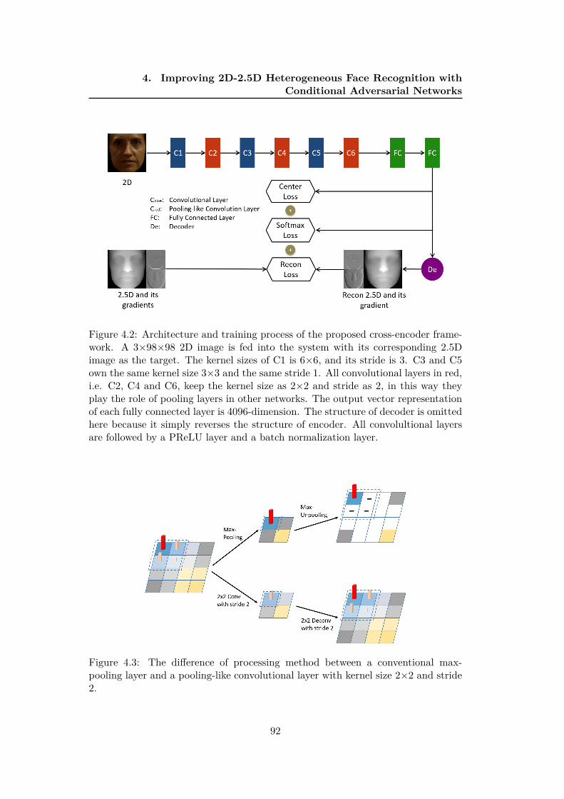
4. Improving 2D-2.5D Heterogeneous Face Recognition withConditional Adversarial Networks
Figure 4.2: Architecture and training process of the proposed cross-encoder frame-work. A 3×98×98 2D image is fed into the system with its corresponding 2.5Dimage as the target. The kernel sizes of C1 is 6×6, and its stride is 3. C3 and C5own the same kernel size 3×3 and the same stride 1. All convolutional layers in red,i.e. C2, C4 and C6, keep the kernel size as 2×2 and stride as 2, in this way theyplay the role of pooling layers in other networks. The output vector representationof each fully connected layer is 4096-dimension. The structure of decoder is omittedhere because it simply reverses the structure of encoder. All convolultional layersare followed by a PReLU layer and a batch normalization layer.
Figure 4.3: The difference of processing method between a conventional max-pooling layer and a pooling-like convolutional layer with kernel size 2×2 and stride2.
92

4. Improving 2D-2.5D Heterogeneous Face Recognition withConditional Adversarial Networks
Figure 4.4: The comparison of outputs with and without the checkerboard arti-facts. The left two images which benefit from well-adapted convolutional kernelsize and gradient loss presents a smoother surface with invisible checkerboard effectcompared with the right-hand side images which results from a conventional CNN.
our work, we use convolutional layer which helps to effectively learn a better
downsampling/upsampling pattern than pooling layer, especially in the up-
sampling stage. A conceptual illustration of how a pooling-like convolutional
layer differs from conventional max-pooling layer is shown in Fig. 4.3.
2. A common observation occurs lately in connection with the ever-advancing
development of feature visualization and other CNN based image genera-
tion techniques: the checkerboard artifacts [Odena et al. 2016]. This strange
pattern seems unfortunately to be a default drawback for all deconvolution
work, however, the effect could be alleviated to a certain extent by some
workarounds. First, to avoid the uneven overlap which is prone to the checker-
board artifact, we carefully design our network to be sure that the kernel
size in each convolutional layer could be divided by the stride and then the
neighboring pixels after upsampling are supposed to be equally rendered. We
subsequently take into account of not only the recovered range image itself
but also its gradient when evaluating the reconstruction performance. With
this step we are capable to impose a smooth prior within this framework
by minimizing the difference between gradient maps of reconstructed 2.5D
and ground truth 2.5D. This additional prior, conjointly with aforementioned
pooling-like convolutional layer, helps to attenuate the checkerboard artifacts
and make the output image naturally smoother, this effect could be intuitively
perceived in right side of Fig. 4.4.
3. Until quite recently, the trend of using deep CNN focus mainly on maximizing
inter-class differences since it was originally designed and optimized for classi-
93
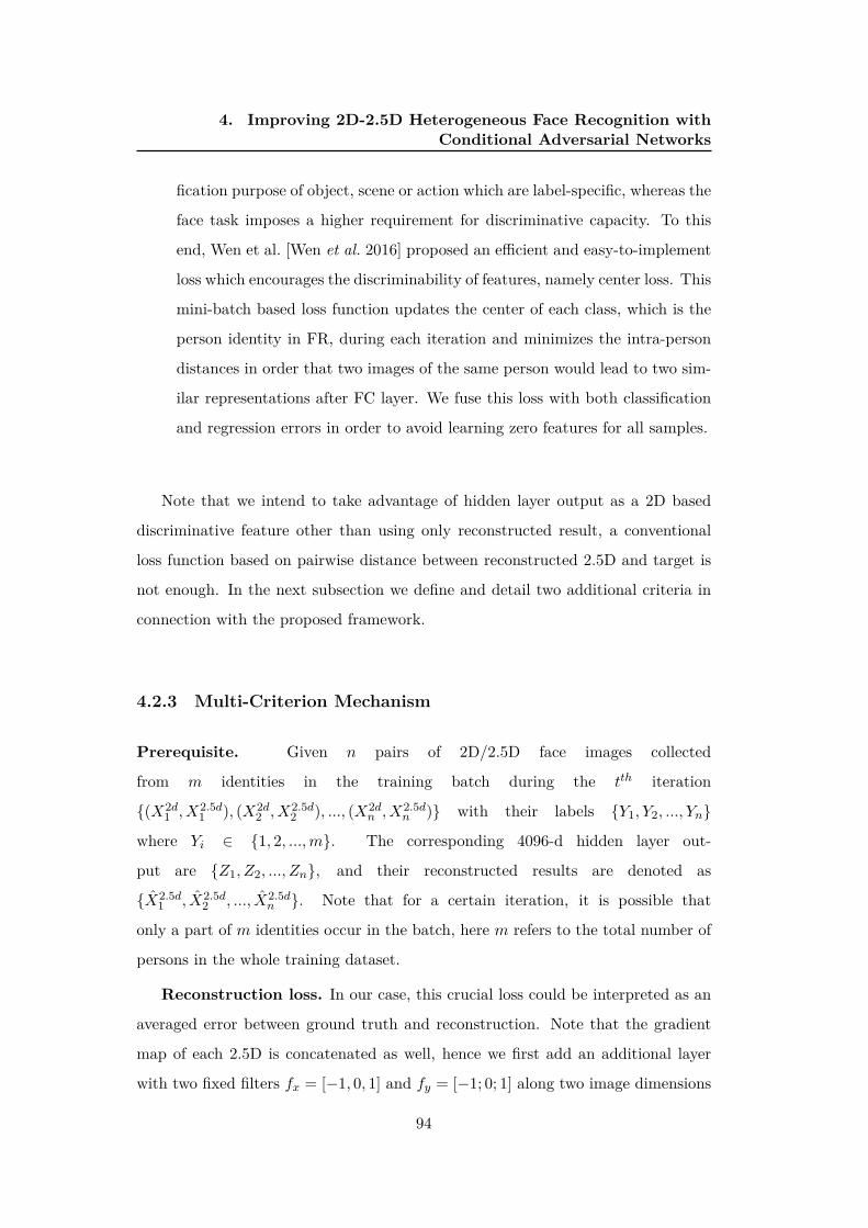
4. Improving 2D-2.5D Heterogeneous Face Recognition withConditional Adversarial Networks
fication purpose of object, scene or action which are label-specific, whereas the
face task imposes a higher requirement for discriminative capacity. To this
end, Wen et al. [Wen et al. 2016] proposed an efficient and easy-to-implement
loss which encourages the discriminability of features, namely center loss. This
mini-batch based loss function updates the center of each class, which is the
person identity in FR, during each iteration and minimizes the intra-person
distances in order that two images of the same person would lead to two sim-
ilar representations after FC layer. We fuse this loss with both classification
and regression errors in order to avoid learning zero features for all samples.
Note that we intend to take advantage of hidden layer output as a 2D based
discriminative feature other than using only reconstructed result, a conventional
loss function based on pairwise distance between reconstructed 2.5D and target is
not enough. In the next subsection we define and detail two additional criteria in
connection with the proposed framework.
4.2.3 Multi-Criterion Mechanism
Prerequisite. Given n pairs of 2D/2.5D face images collected
from m identities in the training batch during the tth iteration
(X2d1 , X2.5d
1 ), (X2d2 , X2.5d
2 ), ..., (X2dn , X2.5d
n ) with their labels Y1, Y2, ..., Yn
where Yi ∈ 1, 2, ...,m. The corresponding 4096-d hidden layer out-
put are Z1, Z2, ..., Zn, and their reconstructed results are denoted as
X2.5d1 , X2.5d
2 , ..., X2.5dn . Note that for a certain iteration, it is possible that
only a part of m identities occur in the batch, here m refers to the total number of
persons in the whole training dataset.
Reconstruction loss. In our case, this crucial loss could be interpreted as an
averaged error between ground truth and reconstruction. Note that the gradient
map of each 2.5D is concatenated as well, hence we first add an additional layer
with two fixed filters fx = [−1, 0, 1] and fy = [−1; 0; 1] along two image dimensions
94
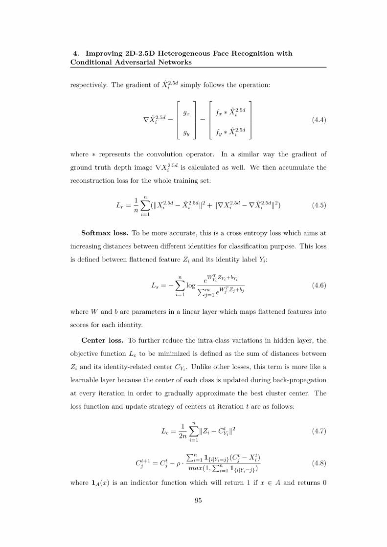
4. Improving 2D-2.5D Heterogeneous Face Recognition withConditional Adversarial Networks
respectively. The gradient of X2.5di simply follows the operation:
∇X2.5di =
gx
gy
=
fx ∗ X2.5di
fy ∗ X2.5di
(4.4)
where ∗ represents the convolution operator. In a similar way the gradient of
ground truth depth image ∇X2.5di is calculated as well. We then accumulate the
reconstruction loss for the whole training set:
Lr =1
n
n∑i=1
(∥X2.5di − X2.5d
i ∥2 + ∥∇X2.5di −∇X2.5d
i ∥2) (4.5)
Softmax loss. To be more accurate, this is a cross entropy loss which aims at
increasing distances between different identities for classification purpose. This loss
is defined between flattened feature Zi and its identity label Yi:
Ls = −n∑
i=1
log eWT
YiZYi
+bYi∑mj=1 e
WTj Zj+bj
(4.6)
where W and b are parameters in a linear layer which maps flattened features into
scores for each identity.
Center loss. To further reduce the intra-class variations in hidden layer, the
objective function Lc to be minimized is defined as the sum of distances between
Zi and its identity-related center CYi . Unlike other losses, this term is more like a
learnable layer because the center of each class is updated during back-propagation
at every iteration in order to gradually approximate the best cluster center. The
loss function and update strategy of centers at iteration t are as follows:
Lc =1
2n
n∑i=1
∥Zi − CtYi∥2 (4.7)
Ct+1j = Ct
j − ρ ·∑n
i=1 1i|Yi=j(Ctj −Xt
i )
max(1,∑n
i=1 1i|Yi=j)(4.8)
where 1A(x) is an indicator function which will return 1 if x ∈ A and returns 0
95

4. Improving 2D-2.5D Heterogeneous Face Recognition withConditional Adversarial Networks
otherwise, ρ denotes the learning rate for updating centers which counteracts the
negative effect of mislabeled samples and outlier data.
The final representation of our loss function combines the above three criteria:
L = Lr + λsLs + λcLc (4.9)
where λs and λc are multipliers for Softmax loss and center loss. The algorithm of
mini-batch gradient descent is further applied to minimize this joint loss.
4.2.4 Heterogeneous Face Recognition
As illustrated in Fig. 4.1, once the proposed discriminative cross-encoder is well
trained, we can extract 2D-based features in the latent feature space while obtaining
reconstructed depth face images with the decoder. To highlight the effectiveness of
this method, we adopt the cosine similarity of 4096-d hidden layer features as 2D-
2D matching scores, the LBP histogram features are extracted from depth images
and Chi-square distance between them is computed as 2.5D-2.5D matching scores.
As for the score fusion stage, all scores are normalized to [0,1] and fused by a simple
sum rule.
4.3 CGAN based HFR Framework
The Cross-encoder is an analysis-by-synthesis approach which can realize the 2D
feature extraction and 2.5D reconstruction simultaneously. Nevertheless, the recon-
struction quality and embedding performance will inevitably impact on each other
while optimizing the joint loss. Moreover, this model requires that both texture and
depth information are provided in the gallery, which is not always fulfilled in real
applications. Hence in this section two novel CNN architectures are proposed to deal
with the reconstruction issue and the HFR issue, respectively. More specifically,
we first formulate our reconstruction problem by adapting it to the background of
cGAN, followed by the detailed cGAN architecture design. Then a two-way CNN
is constructed to map both color image and depth image into a common subspace
96

4. Improving 2D-2.5D Heterogeneous Face Recognition withConditional Adversarial Networks
Figure 4.5: Overview of the proposed CNN models for heterogeneous face recogni-tion. Note that (1) depth recovery is conducted only for testing; (2) the final jointrecognition may or may not include color based matching, depending on the specificexperiment protocol.
for heterogeneous matching. An overview of the proposed approach is given in Fig.
4.5.
4.3.1 Background on CGAN
First proposed in [Goodfellow et al. 2014], Generative Adversarial Network (GAN)
has achieved impressive results in a wide variety of generative tasks. The core idea of
GAN is to train two neural networks, which respectively represent the generator G
and the discriminator D, to proceed a game-theoretic tussle between one another.
Given the samples x from the real data distribution pdata(x) and random noise
z sampled from a noise distribution pz(z), the discriminator aims to distinguish
between real samples x and fake samples which are mapped from z by the generator,
while the generator is tasked with maximally confusing the discriminator. The
objective can thus be written as:
LGAN (G,D) = Ex∼pdata(x)[logD(x)] + Ez∼pz(z)[log(1−D(G(z)))] (4.10)
where E denotes the empirical estimate of expected value of the probability. To
optimize this loss function, we aim to minimize its value for G and maximize it for
97

4. Improving 2D-2.5D Heterogeneous Face Recognition withConditional Adversarial Networks
D in an adversarial way, i.e. minG maxD LGAN (G,D).
The advantage of GAN is that realistic images can be generated from noise
vectors with random distribution, which is crucially important for unsupervised
learning. However, note that in our face recovery scenario, training data contains
image pairs x, y where x and y refer to the depth and color faces respectively with
a one-to-one correspondence between them. The fact that y can be involved in the
model as a prior for generative task leads us to the conditional variant of GAN,
namely cGAN [Mirza & Osindero 2014]. Specifically, we condition the observations
y on both the discriminator and the generator, the objective of cGAN extends Eq.
(4.10) to:
LcGAN (G,D) = Ex,y∼pdata(x,y)[logD(x, y)]+Ez∼pz(z),y∼pdata(y)[log(1−D(G(z|y), y))]
(4.11)
A conceptual working model is illustrated in Fig. 4.6 to help us intuitively un-
derstand how forward-propagation and back-propagation are realized in our cGAN
framework.
Moreover, to ensure the pixel-wise similarity between image generation outputs
G(z|y) and the supervisory signals (ground truth) x, we subsequently impose a
reconstruction constraint on the generator in the form of L1 distance between them:
LL1(G) = Ex,y∼pdata(x,y),z∼pz(z)[∥x−G(z|y)∥1] (4.12)
Here, we adopt the L1 norm instead of the L2 norm for evaluating the reconstruction
error. Despite its popularity as the most commonly used data fidelity constraint in
machine learning, L2 norm arises from the Gaussian assumption of the distribution
and remains easy to solve because it is smooth and convex. However, the L2 norm
fails when dealing with large outliers because it bloats the distance between the
estimate and the outliers. In contrast, as an absolute distance based measure, the
L1 norm is more robust to outliers and has been in use in many recent studies [Wang
et al. 2006,Mehta et al. 2016].
The comprehensive objective is formulated with a minmax value function on the
98
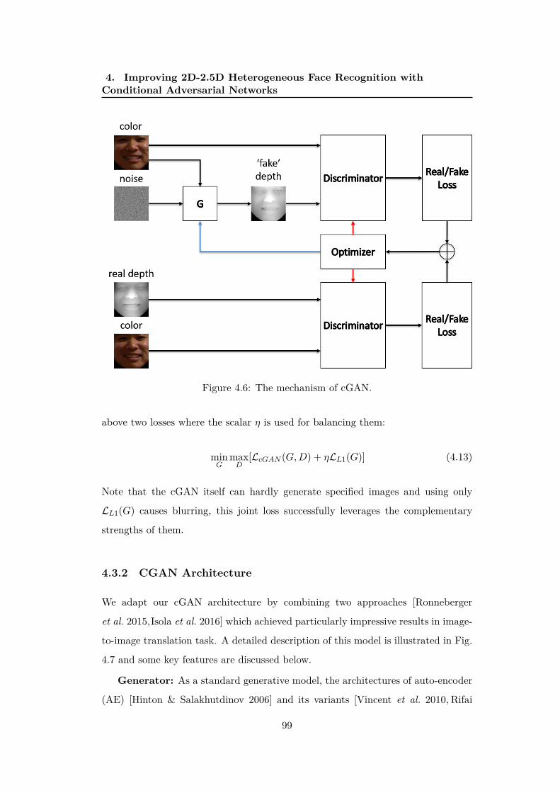
4. Improving 2D-2.5D Heterogeneous Face Recognition withConditional Adversarial Networks
Figure 4.6: The mechanism of cGAN.
above two losses where the scalar η is used for balancing them:
minG
maxD
[LcGAN (G,D) + ηLL1(G)] (4.13)
Note that the cGAN itself can hardly generate specified images and using only
LL1(G) causes blurring, this joint loss successfully leverages the complementary
strengths of them.
4.3.2 CGAN Architecture
We adapt our cGAN architecture by combining two approaches [Ronneberger
et al. 2015,Isola et al. 2016] which achieved particularly impressive results in image-
to-image translation task. A detailed description of this model is illustrated in Fig.
4.7 and some key features are discussed below.
Generator: As a standard generative model, the architectures of auto-encoder
(AE) [Hinton & Salakhutdinov 2006] and its variants [Vincent et al. 2010, Rifai
99

4. Improving 2D-2.5D Heterogeneous Face Recognition withConditional Adversarial Networks
(a)
(b)
Figure 4.7: The architectures of Generator and Discriminator in our cGAN model.In Fig. 4.7a, the noise variable z presents itself under the the form of dropoutlayers, while the black arrows portray the skip connections between encoder layerand decoder layer that are on the ’same’ level. All convolution and deconvolutionlayers are with filter size 4×4 and 1-padding, n and s represent the number ofoutput channels and stride value, respectively. (Best view in color)
100

4. Improving 2D-2.5D Heterogeneous Face Recognition withConditional Adversarial Networks
et al. 2011, Kingma & Welling 2013] are widely adopted as G for past cGANs.
However, the drawback of conventional AEs is obvious: due to their dimension-
ality reduction capacity, a large portion of low-level information, such as precise
localization, is compressed when an image passes through layers in the encoder. To
cope with this lossy compression problem, we follow the idea of U-Net [Ronneberger
et al. 2015] by adding skip connections which forwards directly the features from
encoder layers to decoder layers that are on the same ’level’, as shown in Fig. 4.7a.
The transfer of feature maps at different levels maximally retains the compressed
information during downsampling processes and is therefore capable to produce
precise localizations.
Discriminator: Consistent with Isola et al. [Isola et al. 2016], we adopt
PatchGAN for the discriminator. Within this pattern, no fully connected layers
are implemented and D outputs a 2D image where each pixel represents the predic-
tion result with respect to the corresponding patch on original image. All pixels are
then averaged to decide whether the input image is ’real’ or ’fake’. Compared with
pixel-level prediction, PatchGAN efficiently concentrates on local patterns while
the global low-frequency correctness is enforced by L1 loss in Eq. (4.12).
Optimization: The optimization for cGAN is performed by following the stan-
dard method [Goodfellow et al. 2014]: the mini-batch SGD and the Adam solver
are applied to optimize G and D alternately (as depicted by arrows with different
colors in Fig. 4.6).
4.3.3 Heterogeneous Face Recognition
The reconstruction of depth faces from color images enables us to maximally lever-
age shape information in both gallery and probe, which means we can individually
learn a CNN model to extract discriminative features for depth images and trans-
form the initial cross-modal problem into a multi-modal one. However, the hetero-
geneous matching remains another challenge in our work, below we demonstrate
how this problem is formulated and tackled.
Unimodal learning. The last few years witnessed a surge of interest and
success in FR with deep learning [Taigman et al. 2014, Sun et al. 2015, Parkhi
101

4. Improving 2D-2.5D Heterogeneous Face Recognition withConditional Adversarial Networks
et al. 2015b]. Following the basic idea of stacking convolution-convolution-pooling
(C-C-P) layers, we train from scratch two CNNs for color and grayscale images on
CASIA-WebFace [Yi et al. 2014] and further fine-tune the grayscale based model
with our own depth images. These two models serve two purposes: to extract
2D and 2.5D features individually, and to offer pre-trained models for the ensuing
cross-modal learning.
Cross-modal learning. Once a pair of unimodal models for both views are
trained, the modal-specific representations, X,Y , can be obtained after the last
fully connected layers. Note that each input for the two-stream cross-modal CNN
is a 2D+2.5D image pair with identity correspondence, it is thus reasonable to have
an intuition that X and Y share common patterns which help to classify them
as the same class. This connection essentially reflects the nature of cross-modal
recognition, and was investigated in [Wang et al. 2016, Huang et al. 2012, Wang
et al. 2014].
In order to explore this shared and discriminative feature, a joint supervision
is required to enforce both correlation and distinctiveness simultaneously. For this
purpose, we apply two linear mappings following X and Y , denoted by MX and
MY . First, to ensure the correlation between new features, they are enforced to be
as close as possible, which is constrained by minimizing their distance in feature
space:
Lcorr =
n∑i=1
∥MXXi −MY Yi∥2F (4.14)
where n denotes the size of mini-batch and ∥ · ∥F represents the Frobenius norm.
If we only use the above loss supervision signal, the model will simply learn zero
mappings for MX and MY because the correlation loss will stably be 0 in this case.
To avoid this tricky situation, we average the two outputs to obtain a new feature
on which the classification loss is computed. The ultimate objective function is
102

4. Improving 2D-2.5D Heterogeneous Face Recognition withConditional Adversarial Networks
Figure 4.8: Training procedure of the cross-modal CNN model. Models in thedashed box are pre-trained using 2D and 2.5D face images individually.
formulated as follows:
Lhfr = Lsoftmax + λLCorr
= −n∑
i=1
log eWTci(MXXi+MY Yi)/2+bci∑m
j=1 eWT
j (MXXi+MY Yi)/2+bj+ λ
n∑i=1
∥MXXi −MY Yi∥2F
where ci represents the ground truth class label of ith image pair, the scalar λ
denotes the weight for correlation loss. Fig. 4.8 depicts the above-described training
procedure, including the network details and the joint loss, of the proposed cross-
modality CNN framework. Note that in our work, we will address the 1-N face
identification problem on the FRGC database instead of the 1-1 face verification
problem in other databases such as LFW and Youtube Faces. Hence we decide to
follow the conventional face identification pipeline by adopting a softmax classifier.
There are three main reasons for this decision: 1) softmax is straightforward in
this 1-N identification scenario; 2) it avoids the tricky sampling of image pairs
or triplets as required in some matric learning methods, e.g., triplet loss; 3) to
overcome the over-specialization problem caused by softmax, we do fine-tune the
pre-trained model on the FRGC training set.
Fusion. Being consistent with the previously described HFR pipeline, we adopt
the cosine similarity of 4096-d feature representations as matching scores for 2D-
based, 2.5D-based and 2D/2.5D-based face recognition according to their corre-
sponding networks. All scores are normalized to [0,1] and fused by a simple sum
103

4. Improving 2D-2.5D Heterogeneous Face Recognition withConditional Adversarial Networks
rule.
4.4 Experimental Results
To intuitively demonstrate the effectiveness of the proposed method, we conduct
extensive experiments for 2D/2.5D HFR on the benchmark 2D/2.5D face database.
The evaluations and discussions are not only carried out on the proposed base-
line cross-encoder (hereinafter referred to as baseline-CE) and the cGAN based
framework (hereinafter referred to as cGAN-CE), but also in connection with sev-
eral state-of-the-art methods. The experimental results demonstrated that, while
successfully performing the task of 2.5D depth image recovery, our method also
achieves state-of-the-art performance for 2D/3D HFR.
4.4.1 Dataset Collection
Collecting 2D/2.5D image pairs presents itself as a primary challenge when con-
sidering deep CNN as a learning pipeline. Unlike the tremendous boost in dataset
scale of 2D face images, massive 3D face data acquisition still remains a bottleneck
for the development and practical application of 3D based FR techniques, from
which our work is partly motivated.
Databases: As listed in Table 4.1, three large scale and publicly available 3D
face databases are gathered as training set and the performance is evaluated on
another dataset, which implies that there was no overlap between training and
test set and the generalization capacity of the proposed method is evaluated as
well. Note that the attribute values only concern the data used in our experiments,
for example, scans with large pose variations in CASIA-3D are not included here.
Considering the significance of face alignment and adequate training data, we detail
the preprocessing step and data augmentation method along with the database
overview.
BU3D: BU3D [Yin et al. 2006] was originally constructed for analyzing facial
expressions in 3D space. It contains 2500 two-views’ texture images and 2500
geometric shape models, correspondingly, from 100 female and male subjects with
104
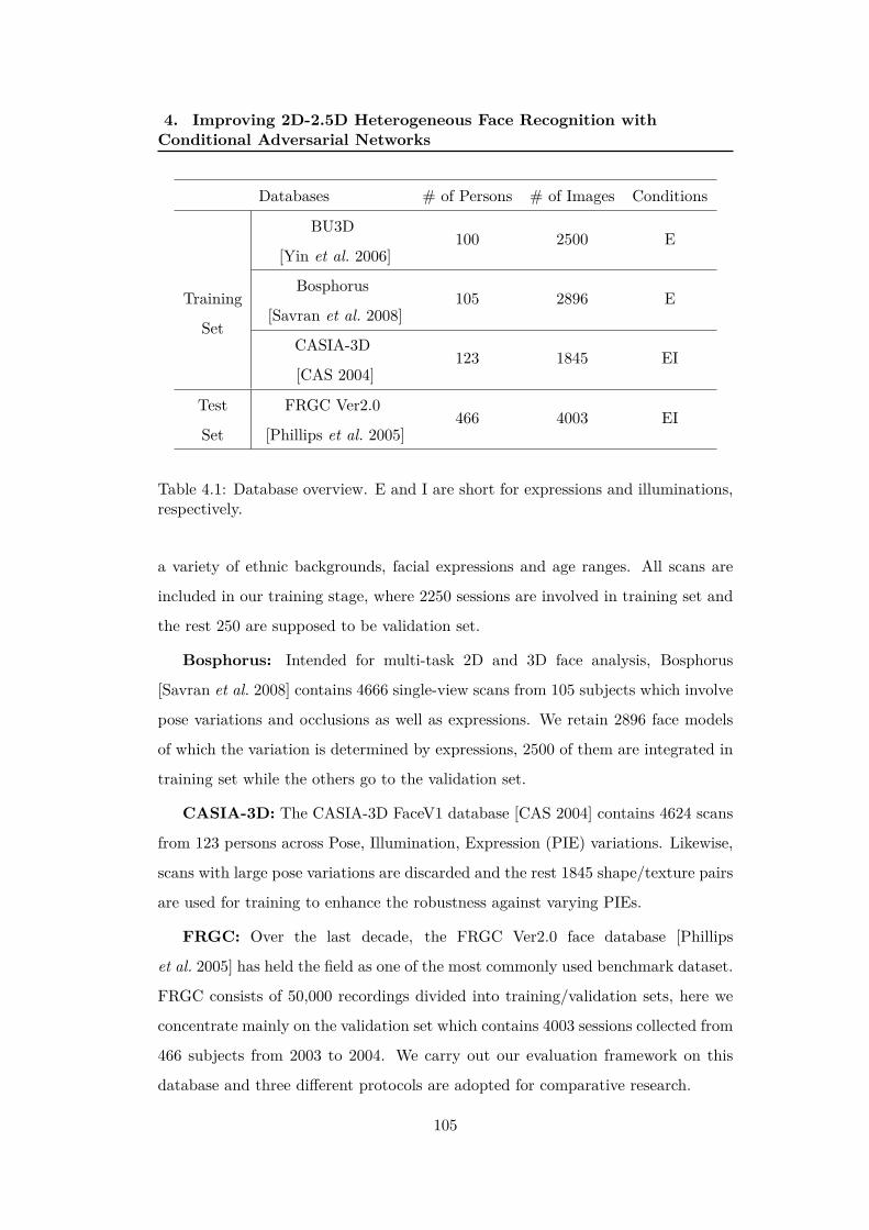
4. Improving 2D-2.5D Heterogeneous Face Recognition withConditional Adversarial Networks
Databases # of Persons # of Images Conditions
Training
Set
BU3D
[Yin et al. 2006]100 2500 E
Bosphorus
[Savran et al. 2008]105 2896 E
CASIA-3D
[CAS 2004]123 1845 EI
Test
Set
FRGC Ver2.0
[Phillips et al. 2005]466 4003 EI
Table 4.1: Database overview. E and I are short for expressions and illuminations,respectively.
a variety of ethnic backgrounds, facial expressions and age ranges. All scans are
included in our training stage, where 2250 sessions are involved in training set and
the rest 250 are supposed to be validation set.
Bosphorus: Intended for multi-task 2D and 3D face analysis, Bosphorus
[Savran et al. 2008] contains 4666 single-view scans from 105 subjects which involve
pose variations and occlusions as well as expressions. We retain 2896 face models
of which the variation is determined by expressions, 2500 of them are integrated in
training set while the others go to the validation set.
CASIA-3D: The CASIA-3D FaceV1 database [CAS 2004] contains 4624 scans
from 123 persons across Pose, Illumination, Expression (PIE) variations. Likewise,
scans with large pose variations are discarded and the rest 1845 shape/texture pairs
are used for training to enhance the robustness against varying PIEs.
FRGC: Over the last decade, the FRGC Ver2.0 face database [Phillips
et al. 2005] has held the field as one of the most commonly used benchmark dataset.
FRGC consists of 50,000 recordings divided into training/validation sets, here we
concentrate mainly on the validation set which contains 4003 sessions collected from
466 subjects from 2003 to 2004. We carry out our evaluation framework on this
database and three different protocols are adopted for comparative research.
105

4. Improving 2D-2.5D Heterogeneous Face Recognition withConditional Adversarial Networks
Figure 4.9: Some face examples of 2D texture and 3D depth image in the FRGCVer2.0 face database. Top: 2D texture samples. Center: 3D depth images beforepreprocessing. Bottom: 3D depth images after filling holes and face region crop-ping. Note that the texture images shown above are correspondingly preprocessedfollowing the same rule with depth images.
Preprocessing: To generate 2.5D range image from original 3D shape, we ei-
ther proceed a direct projection if the point cloud is pre-arranged in grids (Bospho-
rus/FRGC) or adopt a simple Z-buffer algorithm (BU3D/CASIA3D). Furthermore,
to ensure that all faces are of the similar scale, we resize and crop the original im-
age pairs to 98× 98 for baseline-CE and 128× 128 for cGAN-CE while fixing their
inter-ocular distance to a certain value. Especially, to deal with the missing holes
and unwanted body parts (shoulder for example) in raw data of FRGC, we first
locate the face based on 68 automatically detected landmarks [Asthana et al. 2014],
and then apply a linear interpolation to approximate the default value of each hole
pixel by averaging its non-zero neighboring points. Some face samples in FRGC
Ver2.0 before and after preprocessing are illustrated in Fig. 4.9.
106

4. Improving 2D-2.5D Heterogeneous Face Recognition withConditional Adversarial Networks
Data augmentation: Though three mainstream 3D face datasets are gathered
in preparation stage, they are still too few to fit a deep CNN as proposed in our
work. Therefore the data augmentation approach is applied to approximate samples
and thus increase the variability of the original dataset. In this work, we take a few
simple transformations to achieve this goal: 1) horizontal flipping. Each 2D/2.5D
pair is equally flipped in the left-right direction. 2) small amount of shifting. We
iteratively carry out 3×3 1-pixel shiftings around the center area of the image.
4.4.2 Implementation details
All images are normalized before being fed to the network by subtracting from each
channel its mean value over all training data. The baseline-CE and the cGAN-CE
are trained with the architectures as per Section 4.2 and Section 4.3. With regards
to the choice of hyperparameters, unless otherwise specified, we adopt the following
settings:
• In baseline-CE, the learning rate µ begins with 1 and is divided by 5 every
10 epochs, although we found that µ = 1 may cause the loss to explode while
dealing with raw FRGC training set, the preprocessing pipeline solves the
problem perfectly; the momentum m is initially set as 0.5 until it is increased
to 0.9 at the 10th epoch; the weights for Softmax loss λs and center loss λcare respectively set to 0.02 and 0.0001 with the learning rate for updating
class centers ρ = 0.3.
• In cGAN-CE, the learning rate µcGAN is set to 0.0001 and the weight for
L1 norm η is 500; in cross-modal CNN model, the learning rate for training
from scratch µpt begins with 1 and is divided by 5 every 10 epochs while the
learning rate during fine-tuning µft is 0.001; the weight for correlation loss λ
is set to 0.6.
• For all models, the momentum m is initially set as 0.5 until it is increased
to 0.9 at the 10th epoch. Moreover, we adopt Leaky ReLU as the activation
function and implement batch normalization after each convolution layer and
fully connected layer.
107

4. Improving 2D-2.5D Heterogeneous Face Recognition withConditional Adversarial Networks
Figure 4.10: Qualitative reconstruction results of FRGC samples with varying illu-minations and expressions.
4.4.3 Reconstruction Results
The reconstruction results obtained for color images in FRGC are illustrated in Fig.
4.10. Samples from different subjects across expression and illumination variations
are shown from left to right. They thereby give hints on the generalization ability
of the proposed method. For each sample we first portray the original color image
with its ground truth depth image, followed by the reconstructed results with two
proposed methods whereby we demonstrate the effectiveness and necessity of each
constraint in the joint objective.
108

4. Improving 2D-2.5D Heterogeneous Face Recognition withConditional Adversarial Networks
From this figure we can infer that:
1. While being consistently similar with the ground truth, the reconstruction
quality in baseline-CE is far from perfect because a large portion of high-
frequency information is compressed, such as edges and textural details.
2. Compared with the baseline-CE, the cGAN-CE can achieve highly photo-
realistic and accurate reconstruction results, intuitively demonstrating that
the edge-preserving ability of cGAN and the L1-norm data fidelity are effec-
tively integrated in cGAN-CE.
3. The recovered depth faces hold their accuracy and realistic property irrespec-
tive of lighting and expression variations in the original RGB images.
4. A closer examination of results in 3rd and 4th rows provides a further evidence
that the implementation of loss with regard to gradient of 2.5D is beneficial
for obtaining a natural output with few checkerboard artifacts. Meanwhile,
the boundaries between different textures, such as lips, become more consist
with the ground truth.
5. Furthermore, when we take an observation of the two reconstruction results
in 5th and 6th rows, the comparison implies that: 1) using only L1 loss will
lead to blurry results because the model tends to average all plausible values,
especially for regions containing high-level information like edges; 2) using
only cGAN loss can achieve slightly sharper results, but suffers from noise.
These results provide an evidence that the implementation of joint loss is beneficial
and important for obtaining a ’true’ and accurate output.
In addition, some samples with low reconstruction quality in cGAN-CE are
depicted in Fig. 4.11 as well. Obviously, the proposed method encounters some
problems while dealing with extreme cases, such as thick beard, wide opened mouth
and extremely dark shadows as displayed in Fig. 4.11. The errors are principally
due to few training samples with these cases.
109

4. Improving 2D-2.5D Heterogeneous Face Recognition withConditional Adversarial Networks
Figure 4.11: Several wrongly reconstructed samples.
4.4.4 2D-3D Asymmetric FR
We conduct the quantitative experiments on FRGC which has held the field as one
of the most commonly used benchmark dataset over the last decade. In contrast
with unimodal FR experiments, very few attempts have been made on 2D/3D
asymmetric FR. For convenience of comparison, three recent and representative
protocols reported respectively in [Jin et al. 2014], [Huang et al. 2012] and [Wang
et al. 2014] are followed. These protocols mainly differ in gallery and probe settings,
including splitting and modality setup, which are detailed as follows:
• In [Jin et al. 2014], 285 subjects with more than 6 samples are picked out
among which 5 samples of each person are selected for training and the rest
for testing. In the testing phase, the 2D photos are utilized as the gallery set
and their corresponding 3D range images are used as the probe set.
• In [Huang et al. 2012], the first 3D face model with a neutral expression from
each subject formed a gallery set of 466 samples. The remaining texture faces
(4007-466=3541) were treated as probes.
• In [Wang et al. 2014], 300 subjects from FRGCv2.0 are randomly chosen.
110

4. Improving 2D-2.5D Heterogeneous Face Recognition withConditional Adversarial Networks
For each subject, two visible texture images and two corresponding 3D range
images are selected. The whole database is divided into two parts, training
set and testing set. The training set contains the 2D-3D pairs of 225 subjects,
and the testing set includes other 75 subjects.
The comparison results are shown in Table 4.2, through which we could gain
the following observations:
1. The baseline-CE fails to achieve the state-of-the-art performance, especially
when 2D texture images are not given in the gallery set as in the protocols
of [Jin et al. 2014] and [Wang et al. 2014]. This is mainly due to the twofold
objective of this method which attempts to impose constraints on embedding
learning and image generation simultaneously. However, the fusion result in
the protocol of [Huang et al. 2012] shows the effectiveness of cross-encoder
architecture in this specific scenario.
2. The proposed cGAN-CE outperforms state-of-the-art performance while fus-
ing 2.5D matching into HFR with reconstructed depth image further helps
improve the performance effectively. Moreover, the proposed method is ad-
vantageous in its 3D-free reconstruction capacity. To the best of our knowl-
edge, this is the first time to investigate a 2.5D face recovery approach which
is free of any 3D prototype models.
3. Generally, in our proposed cGAN-CE, 2D/2.5D cross-modality matching per-
forms better than 2.5D-based matching, yet achieves slightly lower recogni-
tion accuracy than 2D-based matching. Nevertheless, this does not imply
that cross-modality matching is meaningless compared with 2D-based match-
ing. First, as proven in this table, the heterogeneous matching can be rea-
sonably fused with single modality based matching to further improve the
performance. Then the cross-modality matching can specifically handle the
scenarios where totally different modalities are presented in the gallery and
the probe, which remains an insoluble problem for single modality based ap-
proaches.
111

4. Improving 2D-2.5D Heterogeneous Face Recognition withConditional Adversarial Networks
ProtocolM
ethodsR
ank-1R
ecognitionA
ccuracy
2D2.5D
2D/2.5D
Fusion
Jinet
al.[Jinetal.2014]
MSD
A+
ELM[Jin
etal.2014]-
-0.9680
0.9680
baseline-CE
-0.8849
-0.8849
cGA
N-C
E-
0.95730.9603
0.9698
Wang
etal.[W
angetal.2014]
GR
BM+
rKC
CA
[Wang
etal.2014]-
-0.9600
0.9600
baseline-CE
-0.9115
-0.9115
cGA
N-C
E-
0.95290.9714
0.9745
Huang
etal.[H
uangetal.2012]
OG
M[H
uangetal.2012]
0.9390-
0.94040.9537
baseline-CE
0.94290.9177
-0.9562
cGA
N-C
E0.9755
0.96090.9688
0.9792
Table4.2:
Com
parisonofrecognition
accuracyon
FRG
Cunder
differentprotocols.
Note
thatsom
eblank
numbers
arereported
inthis
tablebecause
westrictly
followthe
protocoldefinedin
eachrelated
literature,e.g.the
galleryset
in[ W
angetal.2014]solely
containsdepth
images,w
hencom
paredw
iththeir
work,ourexperim
entw
illsubsequentlyexclude
2Dbased
matching
torespect
thisprotocol.
112

4. Improving 2D-2.5D Heterogeneous Face Recognition withConditional Adversarial Networks
λ 0 0.2 0.4 0.6 0.8 1 1.2
Accuracy 0.9245 0.9481 0.9600 0.9688 0.9577 0.8851 0.7333
Table 4.3: 2D/2.5D HFR accuracy of cGAN-CE with varying λ under protocolof [Huang et al. 2012].
In addition, despite nearly 20 hours for the whole training and fine-tuning proce-
dure, it takes only 1.6 ms to complete an online forward pass per image on a single
NVIDIA GeForce GTX TITAN X GPU and is therefore capable of satisfying the
real-time processing requirement.
Effect of hyperparameter λ. An extended analysis is made to explore the role
of softmax loss and correlation loss in cGAN-CE. We take the protocol in [Huang
et al. 2012] as a standard and vary the weight for correlation loss λ each time. As
shown in Table 4.3, the performance will remain largely stable across a range of λcbetween 0.4 and 0.8. When we set λ = 0 instead of 0.6, which means correlation
loss is not involved while training, the network can still learn valuable features
with a recognition rate decrease of 4.43%. However, along with the increase of λ,
the performance drops drastically, which implies that a too strong constraint on
correlation loss could lead to side effect by causing a negative impact on softmax
loss.
4.5 Conclusion
In this chapter, we have presented two novel framework for 2D/2.5D heteroge-
neous face recognition together with depth face reconstruction. The first ap-
proach (baseline-CE) extends the Auto-encoder architecture to different input-
output modalities while enforcing the discriminative embedding learning. The sec-
ond approach (cGAN-CE) further combines the generative capacity of conditional
GAN and the discriminative feature extraction of deep CNN for cross-modality
learning. The extensive experiments have convincingly evidenced that the proposed
methods successfully reconstruct realistic 2.5D from single 2D while being adaptive
and sufficient for HFR. Moreover, the cGAN-CE architecture could hopefully be
113

4. Improving 2D-2.5D Heterogeneous Face Recognition withConditional Adversarial Networks
generalized to other heterogeneous FR tasks, such as visible light vs. near-infrared
and 2D vs. forensic sketch, which provides an interesting and promising prospect.
114

5
Conclusion and Future Work
Contents
5.1 Contributions . . . . . . . . . . . . . . . . . . . . . . . . . . . . 116
5.1.1 Improving Shadow Suppression for Illumination Robust Face
Recognition . . . . . . . . . . . . . . . . . . . . . . . . . . . . 116
5.1.2 Improving Heterogeneous Face Recognition with Conditional
Adversarial Networks . . . . . . . . . . . . . . . . . . . . . . 117
5.2 Perspective for Future Directions . . . . . . . . . . . . . . . . 117
5.2.1 Pose Invariant Heterogeneous Face Recognition . . . . . . . . 117
5.2.2 Transfer to Other Heterogeneous Face Recognition Scenarios 118
5.2.3 Integration of Unconstrained Face Recognition Techniques . . 118
while conventional face recognition techniques have achieved quasi-perfect per-
formance in most constrained scenarios, they rely heavily on the strictly controlled
imaging conditions, such as frontal pose, neutral expression, normalized lightings
and homogeneous matching modalities. Unconstrained face recognition is therefore
attracting more and more attention to generalize its exploitation in real-life applica-
tions. In this dissertation we have focused on two main problems in unconstrained
face recognition: illumination variations and heterogeneous matching. With respect
to the illumination processing, we propose to leverage the image formation model
in order to derive a shadow-free representation in chromaticity space, this repre-
sentation can further be used to recover color face images with shadow removal.
To deal with the 2D/3D heterogeneous face recognition problem, we proposed two
approaches based on convolutional neural networks: (i) We present an end-to-end

5. Conclusion and Future Work
network architecture which can learn discriminative feature extraction in the latent
space and reconstruct depth image simultaneously. (ii) We refine the first base-
line framework by separating the reconstruction part and embedding part into two
individual tasks, where the reconstruction task is addressed by introducing the pow-
erful conditional Generative Adversarial Network (cGAN) and the cross-modality
embedding is achieved by another CNN with joint loss. In the last chapter, we
conclude this thesis and list the perspectives of our future works.
5.1 Contributions
5.1.1 Improving Shadow Suppression for Illumination Robust FaceRecognition
In Chapter 3, we proposed a novel shadow removal pipeline in chromaticity space
for improving the performance on illumination-normalized face analysis. This ap-
proach is built upon the Lambertian assumption and explicitly deduce a shadow-free
image presentation. The main contributions consist of: (1) introducing the concept
of chromaticity space in face recognition as a remedy to illumination variations, (2)
achieving an intrinsic face image extraction processing in chromaticity space and (3)
realizing a photo-realistic full color face reconstruction with shadow removal. Over-
all, the proposed approach explores physical interpretations for skin color formation
and extracts illumination-insensitive components which are robust to hard-edged
shadows. Furthermore, the shadow-free image reconstruction in color space enables
us to combine this method with other gray-scale level based lighting processing
techniques. Through both qualitative and quantitative experiments, the proposed
approach is proven to be effective by improving performance for face recognition
across illumination variations on different databases. Meanwhile, it shows a promis-
ing potential in practical applications for its photo-realism and extensibility.
116

5. Conclusion and Future Work
5.1.2 Improving Heterogeneous Face Recognition with ConditionalAdversarial Networks
In Chapter 4, we have presented two novel frameworks for 2D/2.5D heterogeneous
face recognition together with depth face reconstruction. The first method, which
was afterwards considered as a CNN baseline, generalizes the self-reconstruction
ability of Auto-encoder to cross-modality inference. Meanwhile it enforces the la-
tent feature space after the encoder phase to be identity-discriminative. Then, the
second approach combines the generative capacity of conditional GAN and the dis-
criminative feature extraction of deep CNN for cross-modality learning. In contrast
to the baseline cross-encoder method, we first add skip connections between encoder
and decoder layers to preserve low-level image details, then a discriminator serves
as an supervision to ensure the photo-realism of generated depth faces, finally an
individual two-stream cross-modality CNN is learnt to construct a discriminative
common subspace for texture and depth images. The extensive experiments have
convincingly evidenced that the proposed method successfully reconstructs realis-
tic 2.5D from single 2D while being adaptive and sufficient for heterogeneous face
recognition. The main advantages of our proposed methods include: (1) they can
adapt to different scenarios with varying modalities in gallery and probe, (2) the
depth reconstruction ability can transform the cross-modality problem into a multi-
modality one which results in a more flexible recognition stage, (3) the strengths
of CNN are fully leveraged to learn a discriminative embedding for 2D/2.5D pair
input.
5.2 Perspective for Future Directions
In this section, some potential extensive works and future research directions are
presented as follows.
5.2.1 Pose Invariant Heterogeneous Face Recognition
As stated in the introduction of this dissertation, pose variation is another main
challenge as well as lighting variation for current unconstrained face recognition.
117

5. Conclusion and Future Work
Some previous researches have achieved significant progress in pose-invariant 2D
face recognition [Ding et al. 2015,AbdAlmageed et al. 2016] and pose-invariant face
alignment [Zhu et al. 2016,Jourabloo & Liu 2017] while heterogeneous face recogni-
tion across pose variations remains an unsolved issue. Considering that faces with
all possible poses can be synthesized using generic face models, a possible solu-
tion inspired by our proposed CNN model is to construct an end-to-end framework
which aims to learn the mapping from a color face under arbitrary pose to its frontal
counterpart in depth space.
5.2.2 Transfer to Other Heterogeneous Face Recognition Scenarios
In our opinion, the proposed 2D/3D asymmetric face recognition architecture is def-
initely not over-specialized for heterogeneous matching between texture images and
depth images. The abilities of cross-modality reconstruction and common subspace
construction could hopefully be generalized to other heterogeneous face recogni-
tion tasks as well, e.g. visible light images vs. near-infrared images and digital
photographs vs. forensic sketches. Furthermore, a comparative study can be con-
ducted to explore the differences and correlations between varying matching pat-
terns, which provides an interesting and promising prospect.
5.2.3 Integration of Unconstrained Face Recognition Techniques
Up until now, our researches on lighting-insensitive face recognition and 2D/3D
heterogeneous face recognition are independent of each other. Meanwhile, it is
worth mentioning that both our lighting processing method and the proposed HFR
framework can be implemented with computational efficiency at the online stage.
Therefore, further efforts in developing this work may include the design of a com-
prehensive framework or a processing chain which can deal with various uncon-
strained conditions in order to address more complicated face analysis problems in
the wild.
118

6
List of Publications
International peer-reviewed conference:
1. Wuming Zhang and Liming Chen. CrossEncoder: Towards 3D-Free Depth
Face Recovery and Fusion Scheme for Heterogeneous Face Recognition. In
Proceedings of the International Workshop on Representation, analysis and
recognition of shape and motion FroM Image data (RFMI), Savoie, 2017.
(Oral)
2. Wuming Zhang, Xi Zhao, Di Huang, Jean-Marie Morvan, Yunhong Wang
and Liming Chen. Illumination-Normalized Face Recognition Using Chro-
maticity Intrinsic Image. In Proceedings of the IEEE International Confer-
ence on Biometrics (ICB), Phuket, 2015. (Oral)
3. Wuming Zhang, Di Huang, Dimitris Samaras, Jean-Marie Morvan, Yun-
hong Wang and Liming Chen. 3D Assisted Face Recognition via Progressive
Pose Estimation. In Proceedings of the IEEE International Conference on
Image Processing (ICIP), Paris, 2014. (Oral)
4. Xi Zhao, Wuming Zhang, Georgios Evangelopoulos, Di Huang, Shishir K.
Shah, Yunhong Wang, Ioannis A. Kakadiaris and Liming Chen. Benchmark-
ing Asymmetric 3D-2D Face Recognition Systems. In Proceedings of 3D Face
Biometrics Workshop, in conjunction with IEEE International Conference on
Automatic Face and Gesture Recognition (FG), Shanghai, 2013.
Submitted papers under review:

6. List of Publications
1. Wuming Zhang, Xi Zhao, Jean-Marie Morvan, and Liming Chen. Improving
Shadow Suppression for Illumination Robust Face Recognition. Submitted to
IEEE Transactions on Pattern Analysis and Machine Intelligence (TPAMI).
2. Wuming Zhang and Liming Chen. CrossEncoder: Towards 3D-Free Depth
Face Reconstruction and Fusion Scheme for Heterogeneous Face Recognition.
Submitted to IEEE Conference on Automatic Face and Gesture Recognition
(FG).
120

Bibliography
[Abate et al. 2007] Andrea F Abate, Michele Nappi, Daniel Riccio and Gabriele
Sabatino. 2D and 3D face recognition: A survey. Pattern recognition letters,
vol. 28, no. 14, pages 1885–1906, 2007. 86
[AbdAlmageed et al. 2016] Wael AbdAlmageed, Yue Wu, Stephen Rawls, Shai
Harel, Tal Hassner, Iacopo Masi, Jongmoo Choi, Jatuporn Lekust, Jungyeon
Kim, Prem Natarajanet al. Face recognition using deep multi-pose represen-
tations. In Applications of Computer Vision (WACV), 2016 IEEE Winter
Conference on, pages 1–9. IEEE, 2016. 118
[Adini et al. 1997] Yael Adini, Yael Moses and Shimon Ullman. Face recognition:
The problem of compensating for changes in illumination direction. Pattern
Analysis and Machine Intelligence, IEEE Transactions on, vol. 19, no. 7,
pages 721–732, 1997. 12, 33, 50
[Ahonen et al. 2006] Timo Ahonen, Abdenour Hadid and Matti Pietikainen. Face
description with local binary patterns: Application to face recognition. Pat-
tern Analysis and Machine Intelligence, IEEE Transactions on, vol. 28,
no. 12, pages 2037–2041, 2006. 25, 72
[Ahonen et al. 2008] Timo Ahonen, Esa Rahtu, Ville Ojansivu and Janne Heikkila.
Recognition of blurred faces using local phase quantization. In Pattern Recog-
nition, 2008. ICPR 2008. 19th International Conference on, pages 1–4. IEEE,
2008. 72
[Altman 1992] Naomi S Altman. An introduction to kernel and nearest-neighbor
nonparametric regression. The American Statistician, vol. 46, no. 3, pages
175–185, 1992. 10
[Asthana et al. 2014] Akshay Asthana, Stefanos Zafeiriou, Shiyang Cheng and
Maja Pantic. Incremental face alignment in the wild. In Proceedings of

Bibliography
the IEEE Conference on Computer Vision and Pattern Recognition, pages
1859–1866, 2014. 106
[Azeem et al. 2014] Aisha Azeem, Muhammad Sharif, Mudassar Raza and Mar-
ryam Murtaza. A survey: Face recognition techniques under partial occlu-
sion. Int. Arab J. Inf. Technol., vol. 11, no. 1, pages 1–10, 2014. 86
[Bach & Jordan 2002] Francis R Bach and Michael I Jordan. Kernel independent
component analysis. Journal of machine learning research, vol. 3, no. Jul,
pages 1–48, 2002. 25
[Barron & Malik 2015] Jonathan T Barron and Jitendra Malik. Shape, illumina-
tion, and reflectance from shading. Pattern Analysis and Machine Intelli-
gence, IEEE Transactions on, vol. 37, no. 8, pages 1670–1687, 2015. 62
[Barrow & Tenenbaum 1978] H.G. Barrow and J.M. Tenenbaum. Recovering in-
trinsic scene characteristics from images. Computer Vision Systems, vol. 2,
pages 3–26, 1978. 51
[Basri & Jacobs 2003] Ronen Basri and David W Jacobs. Lambertian reflectance
and linear subspaces. Pattern Analysis and Machine Intelligence, IEEE
Transactions on, vol. 25, no. 2, pages 218–233, 2003. 37, 39, 54
[Beigpour & van de Weijer 2011] Shida Beigpour and Joost van de Weijer. Object
recoloring based on intrinsic image estimation. In ICCV, IEEE International
Conference on, pages 327–334. IEEE, 2011. 51
[Belhumeur & Kriegman 1996] Peter N Belhumeur and David J Kriegman. What
is the set of images of an object under all possible lighting conditions? In
Computer Vision and Pattern Recognition, 1996. Proceedings CVPR’96,
1996 IEEE Computer Society Conference on, pages 270–277. IEEE, 1996.
38
[Belhumeur & Kriegman 1998] Peter N Belhumeur and David J Kriegman. What
is the set of images of an object under all possible illumination conditions?
122
Bibliography
International Journal of Computer Vision, vol. 28, no. 3, pages 245–260,
1998. 54
[Belhumeur et al. 1997] Peter N. Belhumeur, João P Hespanha and David J. Krieg-
man. Eigenfaces vs. fisherfaces: Recognition using class specific linear pro-
jection. IEEE Transactions on pattern analysis and machine intelligence,
vol. 19, no. 7, pages 711–720, 1997. 24
[Blanz & Vetter 1999] Volker Blanz and Thomas Vetter. A morphable model for
the synthesis of 3D faces. In Proceedings of the 26th annual conference
on Computer graphics and interactive techniques, pages 187–194. ACM
Press/Addison-Wesley Publishing Co., 1999. 39
[Blanz & Vetter 2003] Volker Blanz and Thomas Vetter. Face recognition based on
fitting a 3D morphable model. IEEE Transactions on pattern analysis and
machine intelligence, vol. 25, no. 9, pages 1063–1074, 2003. 39, 46
[Boutellaa et al. 2015] Elhocine Boutellaa, Abdenour Hadid, Messaoud Bengherabi
and Samy Ait-Aoudia. On the use of Kinect depth data for identity, gender
and ethnicity classification from facial images. Pattern Recognition Letters,
vol. 68, pages 270–277, 2015. 47
[Bowyer et al. 2006] Kevin W Bowyer, Kyong Chang and Patrick Flynn. A survey
of approaches and challenges in 3D and multi-modal 3D+ 2D face recogni-
tion. Computer vision and image understanding, vol. 101, no. 1, pages 1–15,
2006. xv, 18, 86
[Breiman 2001] Leo Breiman. Random forests. Machine learning, vol. 45, no. 1,
pages 5–32, 2001. 10
[Brunelli & Poggio 1993] Roberto Brunelli and Tomaso Poggio. Face recognition:
Features versus templates. IEEE transactions on pattern analysis and ma-
chine intelligence, vol. 15, no. 10, pages 1042–1052, 1993. 26
123

Bibliography
[Cao et al. 2010] Zhimin Cao, Qi Yin, Xiaoou Tang and Jian Sun. Face recognition
with learning-based descriptor. In Computer Vision and Pattern Recognition
(CVPR), 2010 IEEE Conference on, pages 2707–2714. IEEE, 2010. 7
[Cardia Neto & Marana 2015] João Baptista Cardia Neto and Aparecido Nilceu
Marana. 3DLBP and HAOG fusion for face recognition utilizing Kinect as
a 3D scanner. In Proceedings of the 30th Annual ACM Symposium on
Applied Computing, pages 66–73. ACM, 2015. 47
[CAS 2004] CASIA-3D FaceV1 database. http://biometrics.idealtest.org/,
2004. 105
[Chang et al. 2005] Kyong I Chang, Kevin W Bowyer and Patrick J Flynn. An
evaluation of multimodal 2D+ 3D face biometrics. IEEE transactions on
pattern analysis and machine intelligence, vol. 27, no. 4, pages 619–624,
2005. 86
[Chen et al. 2000] Hansen F Chen, Peter N Belhumeur and David W Jacobs. In
search of illumination invariants. In Computer Vision and Pattern Recog-
nition, 2000. Proceedings. IEEE Conference on, volume 1, pages 254–261.
IEEE, 2000. 31
[Chen et al. 2005] Terrence Chen, Wotao Yin, Xiang Sean Zhou, Dorin Comani-
ciu and Thomas S Huang. Illumination normalization for face recognition
and uneven background correction using total variation based image mod-
els. In Computer Vision and Pattern Recognition, 2005. CVPR 2005. IEEE
Computer Society Conference on, volume 2, pages 532–539. IEEE, 2005. 34
[Chen et al. 2006a] Terrence Chen, Wotao Yin, Xiang Sean Zhou, Dorin Comaniciu
and Thomas S Huang. Total variation models for variable lighting face
recognition. Pattern Analysis and Machine Intelligence, IEEE Transactions
on, vol. 28, no. 9, pages 1519–1524, 2006. 51
[Chen et al. 2006b] Weilong Chen, Meng Joo Er and Shiqian Wu. Illumination
compensation and normalization for robust face recognition using discrete
124

Bibliography
cosine transform in logarithm domain. Systems, Man, and Cybernetics,
Part B: Cybernetics, IEEE Transactions on, vol. 36, no. 2, pages 458–466,
2006. 35, 73
[Chin & Kim 2009] Seongah Chin and Kyoung-Yun Kim. Emotional intensity-based
facial expression cloning for low polygonal applications. IEEE Transactions
on Systems, Man, and Cybernetics, Part C (Applications and Reviews),
vol. 39, no. 3, pages 315–330, 2009. 13
[Cho et al. 2014] Hyunjong Cho, Rodney Roberts, Bowon Jung, Okkyung Choi and
Seungbin Moon. An efficient hybrid face recognition algorithm using PCA
and GABOR wavelets. International Journal of Advanced Robotic Systems,
vol. 11, no. 4, page 59, 2014. 27
[Chowdhury et al. 2002] A Roy Chowdhury, Rama Chellappa, Sandeep Krishna-
murthy and Tai Vo. 3D face reconstruction from video using a generic
model. In Multimedia and Expo, 2002. ICME’02. Proceedings. 2002 IEEE
International Conference on, volume 1, pages 449–452. IEEE, 2002. 46
[Corneanu et al. 2016] Ciprian Adrian Corneanu, Marc Oliu Simón, Jeffrey F Cohn
and Sergio Escalera Guerrero. Survey on rgb, 3d, thermal, and multimodal
approaches for facial expression recognition: History, trends, and affect-
related applications. IEEE transactions on pattern analysis and machine
intelligence, vol. 38, no. 8, pages 1548–1568, 2016. 86
[Cortes & Vapnik 1995] Corinna Cortes and Vladimir Vapnik. Support-vector net-
works. Machine learning, vol. 20, no. 3, pages 273–297, 1995. 10
[Ding & Tao 2016] Changxing Ding and Dacheng Tao. A comprehensive survey on
pose-invariant face recognition. ACM Transactions on intelligent systems
and technology (TIST), vol. 7, no. 3, page 37, 2016. 86
[Ding et al. 2015] Changxing Ding, Chang Xu and Dacheng Tao. Multi-task pose-
invariant face recognition. IEEE Transactions on Image Processing, vol. 24,
no. 3, pages 980–993, 2015. 118
125

Bibliography
[Du & Ward 2005] Shan Du and Rabab Ward. Wavelet-based illumination normal-
ization for face recognition. In Image Processing, 2005. ICIP 2005. IEEE
International Conference on, volume 2, pages II–954. IEEE, 2005. 35, 73
[Duc et al. 1999] Benoit Duc, Stefan Fischer and Josef Bigun. Face authentication
with Gabor information on deformable graphs. IEEE Transactions on Image
Processing, vol. 8, no. 4, pages 504–516, 1999. 32
[Fidaleo & Medioni 2007] Douglas Fidaleo and Gérard Medioni. Model-assisted 3d
face reconstruction from video. In International Workshop on Analysis and
Modeling of Faces and Gestures, pages 124–138. Springer, 2007. 46
[Finlayson et al. 2006] Graham D Finlayson, Steven D Hordley, Cheng Lu and
Mark S Drew. On the removal of shadows from images. Pattern Analy-
sis and Machine Intelligence, IEEE Transactions on, vol. 28, no. 1, pages
59–68, 2006. 51, 65
[Finlayson et al. 2009] Graham D Finlayson, Mark S Drew and Cheng Lu. Entropy
minimization for shadow removal. International Journal of Computer Vision,
vol. 85, no. 1, pages 35–57, 2009. 57, 58
[Freedman & Diaconis 1981] David Freedman and Persi Diaconis. On the histogram
as a density estimator: L 2 theory. Probability theory and related fields,
vol. 57, no. 4, pages 453–476, 1981. 62
[Freund & Schapire 1995] Yoav Freund and Robert E Schapire. A desicion-
theoretic generalization of on-line learning and an application to boosting.
In European conference on computational learning theory, pages 23–37.
Springer, 1995. 10
[Funt et al. 1992] Brian V Funt, Mark S Drew and Michael Brockington. Recovering
shading from color images. In ECCV, pages 124–132. Springer, 1992. 58
[Gao & Leung 2002] Yongsheng Gao and Maylor KH Leung. Face recognition using
line edge map. IEEE transactions on pattern analysis and machine intelli-
gence, vol. 24, no. 6, pages 764–779, 2002. 32
126

Bibliography
[Georghiades et al. 2001] Athinodoros S. Georghiades, Peter N. Belhumeur and
David J. Kriegman. From few to many: Illumination cone models for face
recognition under variable lighting and pose. IEEE transactions on pattern
analysis and machine intelligence, vol. 23, no. 6, pages 643–660, 2001. 38
[Goodfellow et al. 2014] Ian Goodfellow, Jean Pouget-Abadie, Mehdi Mirza, Bing
Xu, David Warde-Farley, Sherjil Ozair, Aaron Courville and Yoshua Bengio.
Generative adversarial nets. In Advances in neural information processing
systems, pages 2672–2680, 2014. 88, 97, 101
[Goswami et al. 2014] Gaurav Goswami, Mayank Vatsa and Richa Singh. RGB-D
face recognition with texture and attribute features. IEEE Transactions on
Information Forensics and Security, vol. 9, no. 10, pages 1629–1640, 2014.
47
[Goswami et al. 2016] Gaurav Goswami, Mayank Vatsa and Richa Singh. Face
recognition with RGB-D images using Kinect. In Face Recognition Across
the Imaging Spectrum, pages 281–303. Springer, 2016. 47
[Gu & Kanade 2006] Lie Gu and Takeo Kanade. 3d alignment of face in a single
image. In 2006 IEEE Computer Society Conference on Computer Vision and
Pattern Recognition (CVPR’06), volume 1, pages 1305–1312. IEEE, 2006.
46
[Gu et al. 2015] Jiuxiang Gu, Zhenhua Wang, Jason Kuen, Lianyang Ma, Amir
Shahroudy, Bing Shuai, Ting Liu, Xingxing Wang and Gang Wang. Recent
advances in convolutional neural networks. arXiv preprint arXiv:1512.07108,
2015. 29
[Hallinan et al. 1994] Peter W Hallinanet al. A low-dimensional representation of
human faces for arbitrary lighting conditions. In CVPR, volume 94, pages
995–999, 1994. 37
127

Bibliography
[Han et al. 2013] Hu Han, Shiguang Shan, Xilin Chen and Wen Gao. A comparative
study on illumination preprocessing in face recognition. Pattern Recognition,
vol. 46, no. 6, pages 1691–1699, 2013. xv, 35, 36, 70
[Hanrahan & Krueger 1993] Pat Hanrahan and Wolfgang Krueger. Reflection from
layered surfaces due to subsurface scattering. In Proceedings of the 20th
annual conference on Computer graphics and interactive techniques, pages
165–174. ACM, 1993. 53
[Hardoon et al. 2004] David R Hardoon, Sandor Szedmak and John Shawe-Taylor.
Canonical correlation analysis: An overview with application to learning
methods. Neural computation, vol. 16, no. 12, pages 2639–2664, 2004. 42
[He et al. 2010] Kaiming He, Jian Sun and Xiaoou Tang. Guided image filtering.
In Computer Vision–ECCV 2010, pages 1–14. Springer, 2010. 66
[Hérault & Ans 1984] Jeanny Hérault and Bernard Ans. Réseau de neurones à
synapses modifiables: Décodage de messages sensoriels composites par ap-
prentissage non supervisé et permanent. Comptes rendus des séances de
l’Académie des sciences. Série 3, Sciences de la vie, vol. 299, no. 13, pages
525–528, 1984. 25
[Hesher et al. 2003] Curt Hesher, Anuj Srivastava and Gordon Erlebacher. A novel
technique for face recognition using range imaging. In Signal processing and
its applications, 2003. Proceedings. Seventh international symposium on,
volume 2, pages 201–204. IEEE, 2003. 16
[Hinton & Salakhutdinov 2006] Geoffrey E Hinton and Ruslan R Salakhutdinov.
Reducing the dimensionality of data with neural networks. science, vol. 313,
no. 5786, pages 504–507, 2006. 99
[Hoffmann 2007] Heiko Hoffmann. Kernel PCA for novelty detection. Pattern
Recognition, vol. 40, no. 3, pages 863–874, 2007. 25
[Hotelling 1936] Harold Hotelling. Relations between two sets of variates.
Biometrika, vol. 28, no. 3/4, pages 321–377, 1936. 40
128

Bibliography
[Hoyer 2004] Patrik O Hoyer. Non-negative matrix factorization with sparseness
constraints. The Journal of Machine Learning Research, vol. 5, pages 1457–
1469, 2004. 55
[Huang et al. 2007a] Di Huang, Yunhong Wang and Yiding Wang. A robust method
for near infrared face recognition based on extended local binary pattern.
Advances in Visual Computing, pages 437–446, 2007. 26
[Huang et al. 2007b] Gary B. Huang, Manu Ramesh, Tamara Berg and Erik
Learned-Miller. Labeled Faces in the Wild: A Database for Studying Face
Recognition in Unconstrained Environments. Rapport technique 07-49, Uni-
versity of Massachusetts, Amherst, October 2007. 7
[Huang et al. 2009] Di Huang, Mohsen Ardabilian, Yunhong Wang and Liming
Chen. Asymmetric 3D/2D face recognition based on LBP facial representa-
tion and canonical correlation analysis. In Image Processing (ICIP), 2009
16th IEEE International Conference on, pages 3325–3328. IEEE, 2009. 41
[Huang et al. 2010a] Di Huang, Mohsen Ardabilian, Yunhong Wang and Liming
Chen. Automatic asymmetric 3D-2D face recognition. In Pattern Recog-
nition (ICPR), 2010 20th International Conference on, pages 1225–1228.
IEEE, 2010. 41
[Huang et al. 2010b] Di Huang, Guangpeng Zhang, Mohsen Ardabilian, Yunhong
Wang and Liming Chen. 3D face recognition using distinctiveness enhanced
facial representations and local feature hybrid matching. In Biometrics:
Theory Applications and Systems (BTAS), 2010 Fourth IEEE International
Conference on, pages 1–7. IEEE, 2010. 26
[Huang et al. 2011] Di Huang, Caifeng Shan, Mohsen Ardabilian, Yunhong Wang
and Liming Chen. Local binary patterns and its application to facial image
analysis: a survey. IEEE Transactions on Systems, Man, and Cybernetics,
Part C (Applications and Reviews), vol. 41, no. 6, pages 765–781, 2011. xv,
25, 26
129

Bibliography
[Huang et al. 2012] Di Huang, Mohsen Ardabilian, Yunhong Wang and Liming
Chen. Oriented gradient maps based automatic asymmetric 3D-2D face recog-
nition. In 2012 5th IAPR International Conference on Biometrics (ICB),
pages 125–131. IEEE, 2012. xiii, 27, 42, 46, 87, 102, 110, 111, 112, 113
[Husken et al. 2005] Michael Husken, Michael Brauckmann, Stefan Gehlen and
Christoph Von der Malsburg. Strategies and benefits of fusion of 2D and 3D
face recognition. In Computer Vision and Pattern Recognition-Workshops,
2005. CVPR Workshops. IEEE Computer Society Conference on, pages 174–
174. IEEE, 2005. 86
[Isola et al. 2016] Phillip Isola, Jun-Yan Zhu, Tinghui Zhou and Alexei A Efros.
Image-to-image translation with conditional adversarial networks. arXiv
preprint arXiv:1611.07004, 2016. 99, 101
[Jain et al. 2004] Anil K Jain, Arun Ross and Salil Prabhakar. An introduction to
biometric recognition. IEEE Transactions on circuits and systems for video
technology, vol. 14, no. 1, pages 4–20, 2004. 6
[Jain et al. 2006] Anil Jain, Ruud Bolle and Sharath Pankanti. Biometrics: per-
sonal identification in networked society, volume 479. Springer Science &
Business Media, 2006. 3, 5
[Jin et al. 2014] Yi Jin, Jiuwen Cao, Qiuqi Ruan and Xueqiao Wang. Cross-
modality 2D-3D face recognition via multiview smooth discriminant analysis
based on ELM. Journal of Electrical and Computer Engineering, vol. 2014,
page 21, 2014. xvi, 43, 44, 46, 87, 110, 111, 112
[Jobson et al. 1997a] Daniel J Jobson, Z-U Rahman and Glenn A Woodell. Proper-
ties and performance of a center/surround retinex. Image Processing, IEEE
Transactions on, vol. 6, no. 3, pages 451–462, 1997. 33, 73
[Jobson et al. 1997b] Daniel J Jobson, Zia-ur Rahman and Glenn A Woodell. A
multiscale retinex for bridging the gap between color images and the human
130

Bibliography
observation of scenes. Image Processing, IEEE Transactions on, vol. 6, no. 7,
pages 965–976, 1997. 34, 73
[Jourabloo & Liu 2017] Amin Jourabloo and Xiaoming Liu. Pose-Invariant Face
Alignment via CNN-Based Dense 3D Model Fitting. International Journal
of Computer Vision, pages 1–17, 2017. 118
[Kakadiaris et al. 2007] Ioannis A Kakadiaris, Georgios Passalis, George Toderici,
Mohammed N Murtuza, Yunliang Lu, Nikos Karampatziakis and Theoharis
Theoharis. Three-dimensional face recognition in the presence of facial ex-
pressions: An annotated deformable model approach. IEEE Transactions on
Pattern Analysis and Machine Intelligence, vol. 29, no. 4, 2007. 44
[Kakadiaris et al. 2016] Ioannis A Kakadiaris, George Toderici, Georgios Evan-
gelopoulos, Georgios Passalis, Dat Chu, Xi Zhao, Shishir K Shah and Theo-
haris Theoharis. 3D-2D Face Recognition with Pose and Illumination Nor-
malization. Computer Vision and Image Understanding, 2016. 45, 46, 87
[Kanade 1973] Takeo Kanade. Picture processing system by computer complex
and recognition of human faces. Doctoral dissertation, Kyoto University,
vol. 3952, pages 83–97, 1973. 2
[Kanade 1977] Takeo Kanade. Computer recognition of human faces, volume 47.
Birkhäuser Basel, 1977. 32
[Kee et al. 2000] Seok Cheol Kee, Kyoung Mu Lee and Sang Uk Lee. Illumina-
tion invariant face recognition using photometric stereo. IEICE TRANSAC-
TIONS on Information and Systems, vol. 83, no. 7, pages 1466–1474, 2000.
54
[Kemelmacher-Shlizerman & Basri 2011] Ira Kemelmacher-Shlizerman and Ronen
Basri. 3d face reconstruction from a single image using a single reference
face shape. IEEE Transactions on Pattern Analysis and Machine Intelligence,
vol. 33, no. 2, pages 394–405, 2011. 46
131

Bibliography
[Kim et al. 2013] Dong-Ju Kim, Sang-Heon Lee and Myoung-Kyu Sohn. Face recog-
nition via local directional pattern. International Journal of Security and Its
Applications, vol. 7, no. 2, pages 191–200, 2013. 27
[Kingma & Welling 2013] Diederik P Kingma and Max Welling. Auto-encoding
variational bayes. arXiv preprint arXiv:1312.6114, 2013. 99
[Land & McCann 1971] Edwin H Land and John J McCann. Lightness and retinex
theory. JOSA, vol. 61, no. 1, pages 1–11, 1971. 33, 65
[Lawrence et al. 1997] Steve Lawrence, C Lee Giles, Ah Chung Tsoi and Andrew D
Back. Face recognition: A convolutional neural-network approach. IEEE
transactions on neural networks, vol. 8, no. 1, pages 98–113, 1997. xv, 28,
29
[Le 2013] Quoc V Le. Building high-level features using large scale unsupervised
learning. In 2013 IEEE international conference on acoustics, speech and
signal processing, pages 8595–8598. IEEE, 2013. 90
[Lee & Milios 1990] John C Lee and Evangelos Milios. Matching range images of
human faces. In Computer Vision, 1990. Proceedings, Third International
Conference on, pages 722–726. IEEE, 1990. 16
[Lee et al. 2001] Kuang-Chih Lee, Jeffrey Ho and David Kriegman. Nine points of
light: Acquiring subspaces for face recognition under variable lighting. In
Computer Vision and Pattern Recognition, 2001. CVPR 2001. Proceedings
of the 2001 IEEE Computer Society Conference on, volume 1, pages I–I.
IEEE, 2001. 38
[Lei et al. 2016] Yinjie Lei, Yulan Guo, Munawar Hayat, Mohammed Bennamoun
and Xinzhi Zhou. A Two-Phase Weighted Collaborative Representation for
3D partial face recognition with single sample. Pattern Recognition, vol. 52,
pages 218–237, 2016. xv, 18
[Li 2009] Stan Z Li. Encyclopedia of biometrics: I-z., volume 1. Springer Science
& Business Media, 2009. 19
132

Bibliography
[Liao et al. 2007] Shengcai Liao, Xiangxin Zhu, Zhen Lei, Lun Zhang and Stan Li.
Learning multi-scale block local binary patterns for face recognition. Advances
in biometrics, pages 828–837, 2007. 26
[Liu & Wechsler 2001] Chengjun Liu and Harry Wechsler. A Gabor feature classi-
fier for face recognition. In Computer Vision, 2001. ICCV 2001. Proceedings.
Eighth IEEE International Conference on, volume 2, pages 270–275. IEEE,
2001. 32
[Liu et al. 2015] Jingtuo Liu, Yafeng Deng, Tao Bai, Zhengping Wei and Chang
Huang. Targeting ultimate accuracy: Face recognition via deep embedding.
arXiv preprint arXiv:1506.07310, 2015. 30
[Liu et al. 2016] Feng Liu, Dan Zeng, Qijun Zhao and Xiaoming Liu. Joint face
alignment and 3D face reconstruction. In European Conference on Computer
Vision, pages 545–560. Springer, 2016. 46
[Lowe 2004] David G Lowe. Distinctive image features from scale-invariant key-
points. International journal of computer vision, vol. 60, no. 2, pages 91–110,
2004. 27
[Lyons et al. 1999] Michael J Lyons, Julien Budynek and Shigeru Akamatsu. Au-
tomatic classification of single facial images. IEEE Transactions on Pattern
Analysis and Machine Intelligence, vol. 21, no. 12, pages 1357–1362, 1999.
32
[MacLeod & Boynton 1979] Donald IA MacLeod and Robert M Boynton. Chro-
maticity diagram showing cone excitation by stimuli of equal luminance.
JOSA, vol. 69, no. 8, pages 1183–1186, 1979. 58
[Madooei & Drew 2015] Ali Madooei and Mark S Drew. Detecting specular high-
lights in dermatological images. In Image Processing (ICIP), 2015 IEEE
International Conference on, pages 4357–4360. IEEE, 2015. 55
133

Bibliography
[Makwana 2010] Ramji M Makwana. Illumination invariant face recognition: a
survey of passive methods. Procedia Computer Science, vol. 2, pages 101–
110, 2010. 32
[Masci et al. 2011] Jonathan Masci, Ueli Meier, Dan Cireşan and Jürgen Schmid-
huber. Stacked convolutional auto-encoders for hierarchical feature extrac-
tion. In International Conference on Artificial Neural Networks, pages 52–59.
Springer, 2011. 90
[Matthews et al. 2007] Iain Matthews, Jing Xiao and Simon Baker. 2D vs. 3D
deformable face models: Representational power, construction, and real-
time fitting. International journal of computer vision, vol. 75, no. 1, pages
93–113, 2007. 46
[Maxwell et al. 2008] Bruce A Maxwell, Richard M Friedhoff and Casey A Smith.
A bi-illuminant dichromatic reflection model for understanding images. In
Computer Vision and Pattern Recognition, IEEE Conference on, pages 1–8.
IEEE, 2008. 51
[Medioni & Waupotitsch 2003] Gérard Medioni and Roman Waupotitsch. Face
modeling and recognition in 3-D. In Analysis and Modeling of Faces and
Gestures, 2003. AMFG 2003. IEEE International Workshop on, pages 232–
233. IEEE, 2003. 16
[Mehta et al. 2016] Janki Mehta, Kavya Gupta, Anupriya Gogna, Angshul Ma-
jumdar and Saket Anand. Stacked Robust Autoencoder for Classification. In
International Conference on Neural Information Processing, pages 600–607.
Springer, 2016. 98
[Mian et al. 2007] Ajmal Mian, Mohammed Bennamoun and Robyn Owens. An
efficient multimodal 2D-3D hybrid approach to automatic face recognition.
IEEE transactions on pattern analysis and machine intelligence, vol. 29,
no. 11, 2007. 86
134

Bibliography
[Min et al. 2014] Rui Min, Neslihan Kose and Jean-Luc Dugelay. KinectFaceDB:
A Kinect Database for Face Recognition. Systems, Man, and Cybernetics:
Systems, IEEE Transactions on, vol. 44, no. 11, pages 1534–1548, Nov 2014.
47
[Mirza & Osindero 2014] Mehdi Mirza and Simon Osindero. Conditional generative
adversarial nets. arXiv preprint arXiv:1411.1784, 2014. 88, 98
[Nair & Hinton 2010] Vinod Nair and Geoffrey E Hinton. Rectified linear units
improve restricted boltzmann machines. In Proceedings of the 27th inter-
national conference on machine learning (ICML-10), pages 807–814, 2010.
28
[Odena et al. 2016] Augustus Odena, Vincent Dumoulin and Chris Olah. De-
convolution and Checkerboard Artifacts. http://distill.pub/2016/deconv-
checkerboard/, 2016. 93
[Ojala et al. 2002] Timo Ojala, Matti Pietikainen and Topi Maenpaa. Multiresolu-
tion gray-scale and rotation invariant texture classification with local binary
patterns. Pattern Analysis and Machine Intelligence, IEEE Transactions on,
vol. 24, no. 7, pages 971–987, 2002. 25, 26
[Ojansivu & Heikkilä 2008] Ville Ojansivu and Janne Heikkilä. Blur insensitive tex-
ture classification using local phase quantization. In International conference
on image and signal processing, pages 236–243. Springer, 2008. 27
[Oren & Nayar 1994] Michael Oren and Shree K Nayar. Generalization of Lam-
bert’s reflectance model. In Proceedings of the 21st annual conference on
Computer graphics and interactive techniques, pages 239–246. ACM, 1994.
53
[Park & Jain 2007] Unsang Park and Anil K Jain. 3D model-based face recogni-
tion in video. In International Conference on Biometrics, pages 1085–1094.
Springer, 2007. 46
135

Bibliography
[Parkhi et al. 2015a] O. M. Parkhi, A. Vedaldi and A. Zisserman. Deep Face Recog-
nition. In British Machine Vision Conference, 2015. 72
[Parkhi et al. 2015b] Omkar M Parkhi, Andrea Vedaldi and Andrew Zisserman.
Deep Face Recognition. In BMVC, volume 1, page 6, 2015. 101
[Paysan et al. 2009] Pascal Paysan, Reinhard Knothe, Brian Amberg, Sami Romd-
hani and Thomas Vetter. A 3D face model for pose and illumination invari-
ant face recognition. In Advanced video and signal based surveillance, 2009.
AVSS’09. Sixth IEEE International Conference on, pages 296–301. IEEE,
2009. 39
[Phillips et al. 2005] P Jonathon Phillips, Patrick J Flynn, Todd Scruggs, Kevin W
Bowyer, Jin Chang, Kevin Hoffman, Joe Marques, Jaesik Min and William
Worek. Overview of the face recognition grand challenge. In 2005 IEEE
Computer Society Conference on Computer Vision and Pattern Recognition
(CVPR’05), volume 1, pages 947–954. IEEE, 2005. 70, 105
[Phong 1975] Bui Tuong Phong. Illumination for computer generated pictures.
Communications of the ACM, vol. 18, no. 6, pages 311–317, 1975. 53
[Piotraschke & Blanz 2016] Marcel Piotraschke and Volker Blanz. Automated 3d
face reconstruction from multiple images using quality measures. In Proceed-
ings of the IEEE Conference on Computer Vision and Pattern Recognition,
pages 3418–3427, 2016. 46
[Pizer et al. 1987] Stephen M Pizer, E Philip Amburn, John D Austin, Robert Cro-
martie, Ari Geselowitz, Trey Greer, Bart ter Haar Romeny, John B Zimmer-
man and Karel Zuiderveld. Adaptive histogram equalization and its varia-
tions. Computer vision, graphics, and image processing, vol. 39, no. 3, pages
355–368, 1987. 30
[Quinlan 1986] J. Ross Quinlan. Induction of decision trees. Machine learning,
vol. 1, no. 1, pages 81–106, 1986. 10
136

Bibliography
[Ramamoorthi & Hanrahan 2001] Ravi Ramamoorthi and Pat Hanrahan. On the
relationship between radiance and irradiance: determining the illumination
from images of a convex Lambertian object. JOSA A, vol. 18, no. 10, pages
2448–2459, 2001. 38, 54
[Rifai et al. 2011] Salah Rifai, Pascal Vincent, Xavier Muller, Xavier Glorot and
Yoshua Bengio. Contractive auto-encoders: Explicit invariance during fea-
ture extraction. In Proceedings of the 28th international conference on ma-
chine learning (ICML-11), pages 833–840, 2011. 90, 99
[Ronneberger et al. 2015] Olaf Ronneberger, Philipp Fischer and Thomas Brox. U-
net: Convolutional networks for biomedical image segmentation. In Inter-
national Conference on Medical Image Computing and Computer-Assisted
Intervention, pages 234–241. Springer, 2015. 99, 101
[Roth et al. 2016] Joseph Roth, Yiying Tong and Xiaoming Liu. Adaptive 3D face
reconstruction from unconstrained photo collections. In Proceedings of the
IEEE Conference on Computer Vision and Pattern Recognition, pages 4197–
4206, 2016. 46
[Russakovsky et al. 2015] Olga Russakovsky, Jia Deng, Hao Su, Jonathan Krause,
Sanjeev Satheesh, Sean Ma, Zhiheng Huang, Andrej Karpathy, Aditya
Khosla, Michael Bernstein, Alexander C. Berg and Li Fei-Fei. ImageNet
Large Scale Visual Recognition Challenge. International Journal of Com-
puter Vision (IJCV), vol. 115, no. 3, pages 211–252, 2015. 29
[Savran et al. 2008] Arman Savran, Neşe Alyüz, Hamdi Dibeklioğlu, Oya Çeliktu-
tan, Berk Gökberk, Bülent Sankur and Lale Akarun. Bosphorus database
for 3D face analysis. In European Workshop on Biometrics and Identity
Management, pages 47–56. Springer, 2008. 105
[Scheenstra et al. 2005] Alize Scheenstra, Arnout Ruifrok and Remco Veltkamp. A
survey of 3D face recognition methods. In Audio-and Video-Based Biometric
Person Authentication, pages 325–345. Springer, 2005. 86
137

Bibliography
[Schroff et al. 2015] Florian Schroff, Dmitry Kalenichenko and James Philbin.
Facenet: A unified embedding for face recognition and clustering. In Proceed-
ings of the IEEE Conference on Computer Vision and Pattern Recognition,
pages 815–823, 2015. 7, 30
[Shafer 1985] Steven A Shafer. Using color to separate reflection components. Color
Research & Application, vol. 10, no. 4, pages 210–218, 1985. 54
[Shan et al. 2003] Shiguang Shan, Wen Gao, Bo Cao and Debin Zhao. Illumination
normalization for robust face recognition against varying lighting conditions.
In Analysis and Modeling of Faces and Gestures, IEEE International Work-
shop on, pages 157–164. IEEE, 2003. 30
[Shashua & Riklin-Raviv 2001] Amnon Shashua and Tammy Riklin-Raviv. The
quotient image: Class-based re-rendering and recognition with varying illumi-
nations. IEEE Transactions on Pattern Analysis and Machine Intelligence,
vol. 23, no. 2, pages 129–139, 2001. 34
[Shashua 1997] Amnon Shashua. On photometric issues in 3D visual recognition
from a single 2D image. International Journal of Computer Vision, vol. 21,
no. 1, pages 99–122, 1997. 37
[Sim et al. 2003] Terence Sim, Simon Baker and Maan Bsat. The CMU pose, illumi-
nation, and expression database. Pattern Analysis and Machine Intelligence,
IEEE Transactions on, vol. 25, no. 12, pages 1615–1618, 2003. xv, 12, 70
[Singha et al. 2014] M Singha, Daizy Deb and Sudipta Roy. Hybrid feature extrac-
tion method for partial face recognition. Int. J. Emerg. Technol. Adv. Eng.
Website, vol. 4, pages 308–312, 2014. 27
[Sompura & Gupta 2015] Mithila Sompura and Vinit Gupta. An efficient face
recognition with ANN using hybrid feature extraction methods. International
Journal of Computer Applications, vol. 117, no. 17, 2015. 27
[Song et al. 2015] Shuran Song, Samuel P Lichtenberg and Jianxiong Xiao. Sun
rgb-d: A rgb-d scene understanding benchmark suite. In Proceedings of the
138
Bibliography
IEEE conference on computer vision and pattern recognition, pages 567–576,
2015. 47
[Springenberg et al. 2014] Jost Tobias Springenberg, Alexey Dosovitskiy, Thomas
Brox and Martin Riedmiller. Striving for simplicity: The all convolutional
net. arXiv preprint arXiv:1412.6806, 2014. 91
[Srivastava et al. 2014] Nitish Srivastava, Geoffrey Hinton, Alex Krizhevsky, Ilya
Sutskever and Ruslan Salakhutdinov. Dropout: A simple way to prevent
neural networks from overfitting. The Journal of Machine Learning Research,
vol. 15, no. 1, pages 1929–1958, 2014. 29
[Stan & Anil 2005] Z Li Stan and K Jain Anil. Handbook of face recognition.
Springer, 2005. 55, 86
[Štruc & Pavešic 2011] Vitomir Štruc and Nikola Pavešic. Photometric normaliza-
tion techniques for illumination invariance. Advances in Face Image Analy-
sis: Techniques and Technologies, IGI Global, pages 279–300, 2011. 73
[Sun et al. 2014a] Yi Sun, Yuheng Chen, Xiaogang Wang and Xiaoou Tang. Deep
learning face representation by joint identification-verification. In Advances
in neural information processing systems, pages 1988–1996, 2014. 29
[Sun et al. 2014b] Yi Sun, Xiaogang Wang and Xiaoou Tang. Deep learning face
representation from predicting 10,000 classes. In Proceedings of the IEEE
Conference on Computer Vision and Pattern Recognition, pages 1891–1898,
2014. 29
[Sun et al. 2015] Yi Sun, Ding Liang, Xiaogang Wang and Xiaoou Tang. Deepid3:
Face recognition with very deep neural networks. arXiv preprint
arXiv:1502.00873, 2015. 101
[Sun et al. 2016] Yi Sun, Xiaogang Wang and Xiaoou Tang. Sparsifying neural net-
work connections for face recognition. In Proceedings of the IEEE Conference
on Computer Vision and Pattern Recognition, pages 4856–4864, 2016. 30
139

Bibliography
[Taigman et al. 2014] Yaniv Taigman, Ming Yang, Marc’Aurelio Ranzato and Lior
Wolf. Deepface: Closing the gap to human-level performance in face veri-
fication. In Proceedings of the IEEE Conference on Computer Vision and
Pattern Recognition, pages 1701–1708, 2014. xv, 29, 101
[Tan & Triggs 2010] Xiaoyang Tan and Bill Triggs. Enhanced local texture feature
sets for face recognition under difficult lighting conditions. Image Processing,
IEEE Transactions on, vol. 19, no. 6, pages 1635–1650, 2010. 35, 51, 64, 73
[Tan et al. 2006] Xiaoyang Tan, Songcan Chen, Zhi-Hua Zhou and Fuyan Zhang.
Face recognition from a single image per person: A survey. Pattern recog-
nition, vol. 39, no. 9, pages 1725–1745, 2006. 86
[Toderici et al. 2010] George Toderici, Georgios Passalis, Stefanos Zafeiriou, Geor-
gios Tzimiropoulos, Maria Petrou, Theoharis Theoharis and Ioannis A Kaka-
diaris. Bidirectional relighting for 3D-aided 2D face recognition. In Computer
Vision and Pattern Recognition (CVPR), 2010 IEEE Conference on, pages
2721–2728. IEEE, 2010. xvi, 44, 45, 46, 51, 87
[Turk & Pentland 1991] Matthew Turk and Alex Pentland. Eigenfaces for recog-
nition. Journal of cognitive neuroscience, vol. 3, no. 1, pages 71–86, 1991.
24
[Vincent et al. 2008] Pascal Vincent, Hugo Larochelle, Yoshua Bengio and Pierre-
Antoine Manzagol. Extracting and composing robust features with denoising
autoencoders. In Proceedings of the 25th international conference on Ma-
chine learning, pages 1096–1103. ACM, 2008. 90
[Vincent et al. 2010] Pascal Vincent, Hugo Larochelle, Isabelle Lajoie, Yoshua Ben-
gio and Pierre-Antoine Manzagol. Stacked denoising autoencoders: Learning
useful representations in a deep network with a local denoising criterion.
Journal of Machine Learning Research, vol. 11, no. Dec, pages 3371–3408,
2010. 99
140

Bibliography
[Viola & Jones 2004] Paul Viola and Michael J Jones. Robust real-time face detec-
tion. International journal of computer vision, vol. 57, no. 2, pages 137–154,
2004. 27
[Štruc & Pavešić 2009] Vitomir Štruc and Nikola Pavešić. Gabor-Based Kernel
Partial-Least-Squares Discrimination Features for Face Recognition. Infor-
matica (Vilnius), vol. 20, no. 1, pages 115–138, 2009. 73
[Wang et al. 2004] Haitao Wang, Stan Z Li and Yangsheng Wang. Generalized quo-
tient image. In Computer Vision and Pattern Recognition, IEEE Computer
Society Conference on, volume 2, pages II–498. IEEE, 2004. 34, 73
[Wang et al. 2006] Li Wang, Michael D Gordon and Ji Zhu. Regularized least ab-
solute deviations regression and an efficient algorithm for parameter tuning.
In Data Mining, 2006. ICDM’06. Sixth International Conference on, pages
690–700. IEEE, 2006. 98
[Wang et al. 2009] Yang Wang, Lei Zhang, Zicheng Liu, Gang Hua, Zhen Wen,
Zhengyou Zhang and Dimitris Samaras. Face relighting from a single image
under arbitrary unknown lighting conditions. Pattern Analysis and Machine
Intelligence, IEEE Transactions on, vol. 31, no. 11, pages 1968–1984, 2009.
39
[Wang et al. 2011] Biao Wang, Weifeng Li, Wenming Yang and Qingmin Liao. Illu-
mination normalization based on Weber’s law with application to face recog-
nition. Signal Processing Letters, IEEE, vol. 18, no. 8, pages 462–465, 2011.
32, 73
[Wang et al. 2014] Xiaolong Wang, Vincent Ly, Rui Guo and Chandra Kamb-
hamettu. 2d-3d face recognition via restricted boltzmann machines. In
Computer Vision Theory and Applications (VISAPP), 2014 International
Conference on, volume 2, pages 574–580. IEEE, 2014. xiii, xvi, 42, 43, 46,
102, 110, 111, 112
141

Bibliography
[Wang et al. 2016] Ziyan Wang, Ruogu Lin, Jiwen Lu, Jianjiang Fenget al. Corre-
lated and individual multi-modal deep learning for RGB-D object recognition.
arXiv preprint arXiv:1604.01655, 2016. 102
[Wei & Lai 2004] Shou-Der Wei and Shang-Hong Lai. Robust face recognition under
lighting variations. In Pattern Recognition, 2004. ICPR 2004. Proceedings
of the 17th International Conference on, volume 1, pages 354–357. IEEE,
2004. 32
[Wen et al. 2003] Zhen Wen, Zicheng Liu and Thomas S Huang. Face relighting with
radiance environment maps. In Computer Vision and Pattern Recognition.,
volume 2, pages II–158. IEEE, 2003. 51, 54
[Wen et al. 2016] Yandong Wen, Kaipeng Zhang, Zhifeng Li and Yu Qiao. A Dis-
criminative Feature Learning Approach for Deep Face Recognition. In Eu-
ropean Conference on Computer Vision, pages 499–515. Springer, 2016. 30,
94
[Wu et al. 2016] Yuhang Wu, Shishir K Shah and Ioannis A Kakadiaris. Rendering
or normalization? An analysis of the 3D-aided pose-invariant face recog-
nition. In Identity, Security and Behavior Analysis (ISBA), 2016 IEEE
International Conference on, pages 1–8. IEEE, 2016. 45
[Wyszecki & Stiles 2000] G. Wyszecki and W.S. Stiles. Color science: Concepts and
methods, quantitative data and formulae. Wiley Series in Pure and Applied
Optics. Wiley, 2000. 57
[Xie & Lam 2006] Xudong Xie and Kin-Man Lam. An efficient illumination nor-
malization method for face recognition. Pattern Recognition Letters, vol. 27,
no. 6, pages 609–617, 2006. 31
[Yang et al. 2004] Jian Yang, David Zhang, Alejandro F Frangi and Jing-yu Yang.
Two-dimensional PCA: a new approach to appearance-based face represen-
tation and recognition. IEEE transactions on pattern analysis and machine
intelligence, vol. 26, no. 1, pages 131–137, 2004. 24
142

Bibliography
[Yang et al. 2008] Weilong Yang, Dong Yi, Zhen Lei, Jitao Sang and Stan Z Li. 2D–
3D face matching using CCA. In Automatic Face & Gesture Recognition,
2008. FG’08. 8th IEEE International Conference on, pages 1–6. IEEE, 2008.
xv, 41
[Yi et al. 2014] Dong Yi, Zhen Lei, Shengcai Liao and Stan Z Li. Learning face
representation from scratch. arXiv preprint arXiv:1411.7923, 2014. 102
[Yin et al. 2006] Lijun Yin, Xiaozhou Wei, Yi Sun, Jun Wang and Matthew J
Rosato. A 3D facial expression database for facial behavior research. In 7th
international conference on automatic face and gesture recognition (FGR06),
pages 211–216. IEEE, 2006. 104, 105
[Zeiler & Fergus 2014] Matthew D Zeiler and Rob Fergus. Visualizing and un-
derstanding convolutional networks. In European Conference on Computer
Vision, pages 818–833. Springer, 2014. 91
[Zeiler et al. 2011] Matthew D Zeiler, Graham W Taylor and Rob Fergus. Adaptive
deconvolutional networks for mid and high level feature learning. In 2011
International Conference on Computer Vision, pages 2018–2025. IEEE, 2011.
91
[Zhang & Samaras 2006] Lei Zhang and Dimitris Samaras. Face recognition from a
single training image under arbitrary unknown lighting using spherical har-
monics. IEEE Transactions on Pattern Analysis and Machine Intelligence,
vol. 28, no. 3, pages 351–363, 2006. 39
[Zhang et al. 2005a] Lei Zhang, Sen Wang and Dimitris Samaras. Face synthesis
and recognition from a single image under arbitrary unknown lighting using a
spherical harmonic basis morphable model. In Computer Vision and Pattern
Recognition., volume 2, pages 209–216. IEEE, 2005. 51, 54
[Zhang et al. 2005b] Wenchao Zhang, Shiguang Shan, Wen Gao, Xilin Chen and
Hongming Zhang. Local gabor binary pattern histogram sequence (lgbphs):
A novel non-statistical model for face representation and recognition. In
143

Bibliography
Computer Vision, 2005. ICCV 2005. Tenth IEEE International Conference
on, volume 1, pages 786–791. IEEE, 2005. 72
[Zhang et al. 2009a] Taiping Zhang, Bin Fang, Yuan Yuan, Yuan Yan Tang,
Zhaowei Shang, Donghui Li and Fangnian Lang. Multiscale facial struc-
ture representation for face recognition under varying illumination. Pattern
Recognition, vol. 42, no. 2, pages 251–258, 2009. 35, 73
[Zhang et al. 2009b] Taiping Zhang, Yuan Yan Tang, Bin Fang, Zhaowei Shang and
Xiaoyu Liu. Face recognition under varying illumination using gradientfaces.
Image Processing, IEEE Transactions on, vol. 18, no. 11, pages 2599–2606,
2009. 32, 73
[Zhang et al. 2014] Wuming Zhang, Di Huang, Dimitris Samaras, Morvan Jean-
Marie, Yunhong Wang and Liming Chen. 3D assisted face recognition via
progressive pose estimation. In Image Processing (ICIP), IEEE International
Conference on, pages 728–732, 2014. 45, 46
[Zhao et al. 2003] Wenyi Zhao, Rama Chellappa, P Jonathon Phillips and Azriel
Rosenfeld. Face recognition: A literature survey. ACM computing surveys
(CSUR), vol. 35, no. 4, pages 399–458, 2003. 50, 86
[Zhao et al. 2013] Xi Zhao, Wuming Zhang, Georgios Evangelopoulos, Di Huang,
Shishir K Shah, Yunhong Wang, Ioannis A Kakadiaris and Liming Chen.
Benchmarking asymmetric 3D-2D face recognition systems. In Automatic
Face and Gesture Recognition, IEEE International Conference and Work-
shops on, pages 1–8. IEEE, 2013. 87
[Zhao et al. 2014] X Zhao, G Evangelopoulos, D Chu, S Shah and IA Kakadiaris.
Minimizing Illumination Differences for 3D to 2D Face Recognition Using
Lighting Maps. IEEE transactions on cybernetics, vol. 44, no. 5, pages 725–
736, 2014. 39, 45
[Zhou et al. 2014] Hailing Zhou, Ajmal Mian, Lei Wei, Doug Creighton, Mo Hossny
and Saeid Nahavandi. Recent advances on singlemodal and multimodal face
144

Bibliography
recognition: A survey. IEEE Transactions on Human-Machine Systems,
vol. 44, no. 6, pages 701–716, 2014. 86
[Zhu et al. 2016] Xiangyu Zhu, Zhen Lei, Xiaoming Liu, Hailin Shi and Stan Z Li.
Face alignment across large poses: A 3d solution. In Proceedings of the IEEE
Conference on Computer Vision and Pattern Recognition, pages 146–155,
2016. 118
145


Bibliography
147