Face Recognition with Multilevel B-Splines and SupportVector Machines

Manuele BicegoDipartimento di Informatica

University of VeronaStrada Le Grazie 1537134 Verona - Italia

bicego@sci.univr.it

Gianluca IaconoDipartimento di Informatica

University of VeronaStrada Le Grazie 1537134 Verona - Italia

iacono@sci.univr.it

Vittorio MurinoDipartimento di Informatica

University of VeronaStrada Le Grazie 1537134 Verona - Italia

vittorio.murino@univr.it

ABSTRACTThis paper presents a new face recognition system, basedon Multilevel B-splines and Support Vector Machines. Theidea is to consider face images as heightfields, in which theheight relative to each pixel is given by the correspond-ing gray level. Such heightfields are approximated usingMultilevel B-Splines, and the coefficients of approximationare used as features for the classification process, which isperformed using Support Vector Machines. The proposedapproach was thoroughly tested, using ORL, Yale, Stirlingand Bern face databases. The obtained results are very en-couraging, outperforming traditional methods like eigenface,elastic matching or neural-networks based recognition sys-tems.

Categories and Subject DescriptorsI.5.2 [Pattern Recognition]: Design Methodology—clas-sifier design and evaluation; I.4.9 [Image Processing andComputer Vision]: Applications

General TermsDesign, Performance

KeywordsFace recognition, Support Vector Machines, Multi Level B-splines

1. INTRODUCTIONFace recognition is undoubtedly an interesting research

area, of increasing importance in recent years, due to its ap-plicability as a biometric system in commercial and securityapplications. These systems could be used to prevent unau-thorized access or fraudulent use of ATMs, cellular phones,

Permission to make digital or hard copies of all or part of this work forpersonal or classroom use is granted without fee provided that copies arenot made or distributed for profit or commercial advantage and that copiesbear this notice and the full citation on the first page. To copy otherwise, torepublish, to post on servers or to redistribute to lists, requires prior specificpermission and/or a fee.WBMA’03,November 8, 2003, Berkeley, California, USA.Copyright 2003 ACM 1-58113-779-6/03/00011 ...$5.00.

smart cards, desktop PCs, workstations, and computer net-works. The face recognition system has the appealing char-acteristic of not being an invasive control tool, as comparedwith fingerprint or iris biometric systems.

A large literature is available on this topic: the first ap-proaches, in the 70’s, were based on geometric features [10].In [3], features-based matching and template matching meth-ods were compared. One of the best known face recognitionmethod is the so-called Eigenface method [26, 28, 20, 2, 30],which uses the Principal Component Analysis [8] to projectfaces into a low-dimensional space, where every face can beexpressed as a linear combination of the eigenfaces. Thismethod is not robust against variations of the face orienta-tion and one solution was given by the view-based eigenspacemethod introduced in [22]. Another important approach isElastic Matching [30, 14, 27, 13], introduced to obtain in-variance against expression changes. The idea is to builda lattice on image faces (rigid matching stage), and calcu-late at each point of the lattice a bank of Gabor filters.In case of variations of expression, this lattice can warp toadapt itself to the face (elastic matching stage). Many othermethods have been proposed in the last decade, using dif-ferent techniques, such as Neural Networks [5, 18, 16], orHidden Markov Models [12, 24, 21, 6]. Recently, Indepen-dent Component Analysis was used to project faces into alow-dimensional space, similar to Eigenfaces [29]. Koh etal. [11] use a radial grid mapping centered on the nose toextract a feature vector: in correspondence of each point ofthe grid, the mean value of a circular local patch is calcu-lated and forms an element of the feature vector. Then, thefeature vector is classified by a radial basis function neuralnetwork. Ayinde et al. [1] apply Gabor filters of differentsizes and orientations on face images using rank correlationfor classification.

In this paper, a different approach is proposed. We con-sider the face image as a heightfield, in which the height rel-ative to each pixel is given by the corresponding gray level.This surface is approximated using Multilevel B-Splines [17],an interpolation and approximation technique for scattereddata. The resulting approximation coefficients were used asfeatures for the classification, carried out by the SupportVector Machines (SVM) [4]. This classifier has already beenapplied to the face recognition problem [7], in order to clas-sify Principal Components of faces, obtaining very promisingresults. Moreover, the use of the Support Vector Machinesin the context of face authentication has been investigated

in [9].The reasons underlying the choice of using Multilevel B-

Splines and Support Vector Machines are the following: fromone hand, Multilevel B-Splines coefficients have been chosenfor their approximation capabilities, able to manage slightchanges in facial expression. On the other hand, even ifa considerable dimensionality reduction is obtained by thistechnique with respect to considering the whole image, theresulting space is still large. Standard classifiers could beaffected by the so called curse of dimensionality problem;SVMs, instead, are well suited to work in very high dimen-sional spaces (see for example [23]).

The proposed approach was thoroughly tested using mostpopular databases, such as ORL, Yale, Stirling and Bern1,and compared with several different approaches. As shownin the experimental section, results obtained are very en-couraging, outperforming traditional methods like eigenface,elastic matching and neural-networks based recognition sys-tem. Classification accuracies of our approach also outper-form those proposed in [7], where SVMs are used with PCAcoefficients as features, showing that Multilevel B-splines arevery effective and accurate features, able to properly char-acterize face images.

The rest of the paper is organized as follows. Section 2contains theoretical background about Multilevel B-Splinesand Section 3 is dedicated to Support Vector Machines de-scription. In Section 4 the proposed strategy is detailed andexperimental results, including a comparative analysis withdifferent methods and several face databases, are reportedin Section 5. In Section 6 conclusions are finally drawn.

2. MULTILEVEL B-SPLINESThe Multilevel B-Splines [17] represent an approximation

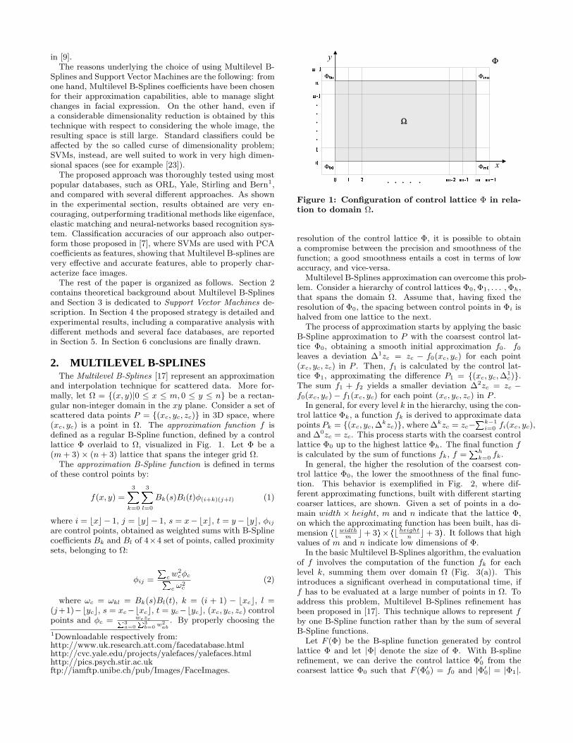
and interpolation technique for scattered data. More for-mally, let Ω = (x, y)|0 ≤ x ≤ m, 0 ≤ y ≤ n be a rectan-gular non-integer domain in the xy plane. Consider a set ofscattered data points P = (xc, yc, zc) in 3D space, where(xc, yc) is a point in Ω. The approximation function f isdefined as a regular B-Spline function, defined by a controllattice Φ overlaid to Ω, visualized in Fig. 1. Let Φ be a(m + 3)× (n + 3) lattice that spans the integer grid Ω.

The approximation B-Spline function is defined in termsof these control points by:

f(x, y) =

3Xk=0

3Xl=0

Bk(s)Bl(t)φ(i+k)(j+l) (1)

where i = bxc− 1, j = byc− 1, s = x−bxc, t = y−byc, φij

are control points, obtained as weighted sums with B-Splinecoefficients Bk and Bl of 4×4 set of points, called proximitysets, belonging to Ω:

φij =

Pc w2

cφcPc ω2

c

(2)

where ωc = ωkl = Bk(s)Bl(t), k = (i + 1) − bxcc, l =(j+1)−bycc, s = xc−bxcc, t = yc−bycc, (xc, yc, zc) controlpoints and φc = wczcP3

a=0P3

b=0 w2ab

. By properly choosing the

1Downloadable respectively from:http://www.uk.research.att.com/facedatabase.htmlhttp://cvc.yale.edu/projects/yalefaces/yalefaces.htmlhttp://pics.psych.stir.ac.ukftp://iamftp.unibe.ch/pub/Images/FaceImages.

Figure 1: Configuration of control lattice Φ in rela-tion to domain Ω.

resolution of the control lattice Φ, it is possible to obtaina compromise between the precision and smoothness of thefunction; a good smoothness entails a cost in terms of lowaccuracy, and vice-versa.

Multilevel B-Splines approximation can overcome this prob-lem. Consider a hierarchy of control lattices Φ0, Φ1, . . . , Φh,that spans the domain Ω. Assume that, having fixed theresolution of Φ0, the spacing between control points in Φi ishalved from one lattice to the next.

The process of approximation starts by applying the basicB-Spline approximation to P with the coarsest control lat-tice Φ0, obtaining a smooth initial approximation f0. f0

leaves a deviation ∆1zc = zc − f0(xc, yc) for each point(xc, yc, zc) in P . Then, f1 is calculated by the control lat-tice Φ1, approximating the difference P1 = (xc, yc, ∆

1c).

The sum f1 + f2 yields a smaller deviation ∆2zc = zc −f0(xc, yc)− f1(xc, yc) for each point (xc, yc, zc) in P .

In general, for every level k in the hierarchy, using the con-trol lattice Φk, a function fk is derived to approximate datapoints Pk = (xc, yc, ∆

kzc), where ∆kzc = zc−Pk−1

i=0 fi(xc, yc),and ∆0zc = zc. This process starts with the coarsest controllattice Φ0 up to the highest lattice Φh. The final function fis calculated by the sum of functions fk, f =

Phk=0 fk.

In general, the higher the resolution of the coarsest con-trol lattice Φ0, the lower the smoothness of the final func-tion. This behavior is exemplified in Fig. 2, where dif-ferent approximating functions, built with different startingcoarser lattices, are shown. Given a set of points in a do-main width × height, m and n indicate that the lattice Φ,on which the approximating function has been built, has di-mension

bwidthm

c+ 3× bheight

nc+ 3

. It follows that high

values of m and n indicate low dimensions of Φ.In the basic Multilevel B-Splines algorithm, the evaluation

of f involves the computation of the function fk for eachlevel k, summing them over domain Ω (Fig. 3(a)). Thisintroduces a significant overhead in computational time, iff has to be evaluated at a large number of points in Ω. Toaddress this problem, Multilevel B-Splines refinement hasbeen proposed in [17]. This technique allows to represent fby one B-Spline function rather than by the sum of severalB-Spline functions.

Let F (Φ) be the B-spline function generated by controllattice Φ and let |Φ| denote the size of Φ. With B-splinerefinement, we can derive the control lattice Φ′0 from thecoarsest lattice Φ0 such that F (Φ′0) = f0 and |Φ′0| = |Φ1|.

Figure 2: Examples of Multilevel B-Splines approx-imation, using different resolutions (m and n) of thefirst control lattice Φ0.

Then, the sum of functions f0 and f1 can be represented bycontrol lattice Ψ1 which results from the addition of eachcorresponding pair of control points in Φ′0 and Φ1. That is,F (Ψ1) = g1 = f0 + f1, where Ψ1 = Φ′0 + Φ1.

In general, let gk =Pk

i=0 fi be the partial sum of func-tions fi up to level k in the hierarchy. Suppose that func-tion gk−1 is represented by a control lattice Ψk−1 such that|Ψk−1| = |Φk−1|. In the same manner as we computed Ψ1

above, we can refine Ψk−1 to obtain Ψ′k−1 , and add Ψ′k−1

to Φk to derive Ψk such that F (Ψk) = gk and |Ψk| = |Φk|. That is, Ψk = Ψ′k−1 + Φk . Therefore, from g0 = f0 andΨ0 = Φ0 , we can compute a sequence of control latticesΨk to progressively derive control lattice Ψh for the finalapproximation function f = gh. A scheme of this procedureis shown in Fig. 3(b).

3. SUPPORT VECTOR MACHINESSupport Vector Machines [4] are binary classifiers, able to

separate two classes through an optimal hyperplane. Theoptimal hyperplane is the one maximizing the “margin”,defined as the distance between the closest examples of dif-ferent classes. To obtain a non-linear decision surface, it ispossible to use kernel functions, in order to project data in ahigh dimensional space, where a hyperplane can more easilyseparate them. The corresponding decision surface in theoriginal space is not linear.

The rest of this section details the theoretical and practi-cal aspects of Support Vector Machines: firstly, linear SVMsare introduced, for both linearly and not linearly separabledata. Subsequently, we introduce non linear SVMs, able toproduce non linear separation surfaces. A very useful andintroductory tutorial on Support Vector Machines for Pat-tern Recognition can be found in [4].

In the case of linearly separable data, let D = (xi, yi), i =1 . . . `, yi ∈ −1, +1,xi ∈ <d be the training set of theSVMs. D is linearly separable if exists w ∈ <d and b ∈ <,such that:

yi(xi ·w + b) ≥ 1 for i = 1, . . . , ` (3)

H : w · x + b = 0 is called the “separating hyperplane”.Let d+(d−) be the minimum distance of the separating hy-perplane from the closest positive (negative) point. Let usdefine the “margin” of the hyperplane as d+ +d−. Different

Φ0

Φ1

Φ2

Φ3

Approximateresidues

Approximateresidues

Approximateresidues

First coarsest approximation

Originalimage

refine

refine

refine

+

+

+

=

Ψ0

Ψ1

Ψ2

Ψ3

evaluate

=

=

=

Finalapproximation

function f

(a)Hierarchyof control

lattices

Sequence of B-Splinefunctions

Φ0

Φ1

Φ2

Φ3

f 0

f 1

f 2

f 3

Finalapproximation

function f

+

+

+

=

Approximateresidues

Approximateresidues

Approximateresidues

First coarsest approximation

Originalimage

evaluate

evaluate

evaluate

evaluate

(b)

Figure 3: Description of MBA algorithm: (a) basicversion; (b) MBA with refinement.

Origin

W

H2

H1

Margin|| Wb−

Figure 4: Geometric interpretation of SVMs. A hy-perplane separates black points from white points.The hyperplane is obtained as a linear combinationof the circled points, called support vectors, and isdefined by a direction vector W and a distance-from-origin scalar b.

separating hyperplanes exist. SVMs find the one that max-imizes the margin. Let us define H1 : w · x + b = +1 andH2 : w · x + b = −1. The distance of a point of H1 from

H : w ·x+b = 0 is |w·x+b|‖w‖ = 1

‖w‖ , and the distance between

H1 and H2 is 2‖w‖ . So, to maximize the margin, we must

minimize ‖w‖ = wT w, with the constraints that no pointslie between H1 and H2.

It can be proven [4] that the problem of training a SVMis reduced to the solution of the following Quadratic Pro-gramming (QP) problem:

max−1

2αT Bα +

Xi=1

αi (4)

Xi=1

yiαi = 0 and αi ≥ 0 (5)

where αi are Lagrange coefficients and B is a ` × ` matrixdefined as:

Bij = yiyjxi · xj (6)

The optimal hyperplane is determined with w =P`

i=1 αiyixi,and the classification of a new point x is obtained by calcu-lating sgn(w · x + b). It is important to observe that onlythose xi whose corresponding Lagrange coefficients αi arenot null contribute to the sum that defines the separatinghyperplane. For this reason, these points are called supportvectors and, geometrically, lie along the two hyperplanes H1

and H2 (see the Fig. 4). When data points are not linearlyseparable, slack variables are introduced, in order to allowpoints to exceed margin borders:

yi(xi ·w + b) ≥ 1− ξi (7)

The idea is to permit such situations, by controlling themby the introduction of a cost parameter C. This parame-ter determines the sensibility of the SVM to classificationerrors: a high value of C strongly penalizes errors, also atthe cost of a narrow margin, while a low value of C permitssome classification errors. Intermediate values of C result ina compromise between the minimization of the number of

errors and maximization of the margin. Finally, the trainingprocess results in the solution of the following QP problem:

maxX

i

αi − 1

2

Xi,j

αiαjyiyjxi · xj (8)

Xi=1

yiαi = 0 and 0 ≤ αi ≤ C (9)

The SVM approach could also be generalized to the casewhere the decision function is not a linear function of thedata: in this case we have the so-called non-linear SVM. Theidea under nonlinear SVMs is to project data points into ahigh, even huge, dimensional Hilbert space H, by using afunction Ξ such that:

Ξ : <d → H

x → z(x) = z(ξ1(x), ξ2(x), . . . , ξn(x))

and then separate projected data points through a hyper-plane.

First of all, notice that the only way in which the dataappear in the training problem is in the form of inner prod-ucts xi · xj. When projecting points x in Ξ(x), the trainingprocess will still depend on the inner product of projectedpoints Ξ(xi) ·Ξ(xj). Then, to solve the problem of nonlineardecision surfaces, it is sufficient to modify the training andclassification algorithms, substituting the inner product be-tween data points of the training set with a kernel functionK, such that:

K(xi,xj) = Ξ(xi) · Ξ(xj) (10)

To be a kernel, a function must verify Mercer conditions[4]. Some examples of kernel are polynomial functions likeK(x, y) = ((x ·y)+1)d, exponential radial basis function andmulti-layer perceptron. In this way, data points are projectedin a higher dimensional space, where a hyperplane could besufficient to separate the problem properly. It is importantto notice that, by the use of this “kernel trick”, the non lineardecision surface is obtained in roughly the same amount oftime needed to build a linear SVM.

4. THE STRATEGYIn this section, the proposed strategy is detailed: features

are extracted using Multilevel B-Splines, and successivelyclassified using Support Vector Machines.

First, the face image should be sampled, in order to obtaina set of points to approximate. This set is obtained by thefusion of two subsets: firstly, a Canny filter is applied to ex-tract edges from the image faces. Therefore, the first subsetof control points to approximate is P1 = (xc1 , yc1 , zc1), withxc1 , yc1 coordinates of the edges and zc1 the correspondinggray levels. The second subset of control points is given byP2 = (xc2 , yc2 , zc2), with xc2 , yc2 coordinates correspondingto a sub-sampling carried out on the image. Finally, the setof control points to approximate is given by P = P1 ∪ P2,as shown in Fig. 5(b) as an example. Subsequently, the ap-proximation algorithm is applied to this set of points, con-sidering the control lattice coefficients as features. Once ex-tracted, the control lattice is linearized into a feature vector,using the standard raster scan.

Face recognition is a multi-class classification problem,but Support Vector Machines are binary classifiers. To ex-

Figure 5: Feature extraction stage. Original faceimage and used control points.

tend SVMs to the multi-class case, we adopted the strategyof binary decision trees proposed by Verri et al. [23], alsocalled strategy of the tennis tournament, also adopted byGuo et al. in their paper [7].

Let us assume to have c classes. The training stage con-sists in building up all possible SVMs 1-vs-12, combiningall the available classes. The number of possible (not or-

dered) pairs of classes is c(c−1)2

. In this way, c(c−1)2

SVMsare trained. In the classification stage, a binary decisiontree is built, starting from the leaves, in which each pair ofbrother nodes represent a SVM. Given a test image, recog-nition was performed following the rules of a tennis tourna-ment. Each class is regarded as a player, and in each matchthe system classifies the test images according to the deci-sion of the SVM of the pair of players involved in the match.The winner identities, proposed by each SVM, will be prop-agated to the upper level of the tree, playing again. Theprocess continues until the root is reached. Finally, the rootwill be labelled with the identity of the classified subject.Because it is a priori impossible to know which SVM willdefine the various levels of the tree, the necessity of trainingall possible SVMs 1-vs-1 is now clear.

In Fig. 6, an example of this classification rule is proposed.In principle, different choices of the starting configuration,regarding SVMs inserted as leaves, could lead to differentresults. Nevertheless, in practice, preliminary experimentsshowed that averaged accuracies do not depend from thestarting configuration.

If c does not equal to the power of 2, we can decompose cas: c = 2n1 +2n2 + . . .+2nI , where n1 ≥ n2 ≥ . . . ≥ nI . If cis an odd number, nI = 0; otherwise, nI > 0. Then, we canbuild I trees, the first with n1 leaves, the second with n2 andso on. Finally, starting from the I roots, we can build thefinal tree (or, if necessary, recursively decompose I again inpowers of 2). Even if this decomposition is not unique, thenumber of comparisons in the classification stage is alwaysc− 1.

5. EXPERIMENTAL RESULTSIn this section, experimental results are proposed. We

preliminary studied three different types of approximationcoefficients as features, regarding three different methods

2We call this kind of SVMs 1-vs-1, in order to distinguishthem from SVMs 1-vs-all, that were trained to classify be-tween faces of one class and faces of all other classes.

1 2 43 5 6 7 8

1 3 6 7

1 6

1

Figure 6: An example of multi-class classifica-tion.The subject to be recognized belongs to classnumber 1. First, it is classified by the SVM relativeto classes 1-2, 3-4, 5-6, 7-8. The winners of this firstset of classifications will define the upper level of thetree, constituted by SVMs relative to pairs 1-3 and6-7. Finally, the final SVM relative to classes 1 and6 establishes the winner.

Database N.subj N.training N.testingORL 40 5 5Yale 15 5 6

Stirling 32 3 3Bern 30 5 5

Combined 117 Variable Variable

Table 1: Description of the databases used for ex-periments: number of subjects, photos per subjectused for training and for testing.

to approximate points: B-splines, Multilevel B-splines, andMultilevel B-splines with refinement. The features we inves-tigated were therefore: the φij ’s calculated with the B-Splineapproximation method under different resolutions, the φij ’sof the control lattice hierarchy calculated with the Multi-level B-Splines algorithm, and the ψij ’s calculated with theMultilevel B-Splines algorithm with refinement. This lastalgorithm obtained the best results, in terms of recognitionrate: therefore, in the following, only results regarding thisalgorithm are proposed.

About the kernel used in Support Vector Machine, af-ter several experimental tests, the best performance wasreached by the Exponential Radial Basis Function, whichprovided the most stable results. In our experiments the pa-rameters of the SVMs were set to C = 100 and σ = 20, withσ the kernel variance, being the results stable for C ≥ 100and σ ≥ 20.

We used different face databases to test the proposed sys-tem. Databases, number of subjects and photos per subjectsused in the training and testing set, are shown in Table 1.Moreover, in this table, “combined” means a database ob-tained by the fusion of all other databases. We tested dif-ferent random combinations of training and testing sets andresults were averaged. All face images were resized to thedimensions of ORL databases photos, i.e. 92× 112 pixel.

Some comments about the databases used: ORL databasecontains a high within-class variance, like illumination changes,facial expressions, glasses/no glasses, and scale. Subjectsin the Yale database are characterized by high illumination

Level MBA-REF BA32 4.25% 4.25%16 2.75% 3.13%8 3.75% 4%4 3.88% 4.25%2 4.13% 4.13%

Database ErrorsYale 1.11%

Stirling 1.04%Bern 4.67%

Combined 3.3%

(a) (b)

Table 2: Recognition error rates: (a) on ORLdatabase, with different resolutions of the controllattice used as features vector. MBA-REF stands forMultilevel B-Splines approximation with refinementand BA stands for basic B-Splines approximation;(b) on other databases, with Multilevel B-Splineswith refinement and level 16.

changes, presence and absence of glasses, and variations infacial expressions. Stirling database contains subjects in var-ious poses and expressions (smiling and speaking). Finally,Bern database presents photos under partially controlled il-lumination conditions, but with different poses.

In Table 2(a), classification error rates calculated on ORLface database are shown. With the aim of understandinghow to exploit the multi-level nature of the described algo-rithms, the system performances on this database are pro-posed for different levels of resolution of the control lattice.We recall that “level n” means dimensionality of the con-trol lattice Φ equal to

bheightn

c+ 3× bwidth

nc+ 3

, where

height and width are relative to image dimensions. More-over, in Table 2(a) a comparison between coefficients of Mul-tilevel B-Splines with refinement and basic B-Spline approx-imation as features is shown. It can be noticed how theformers obtain a better performance.

One can note that results are very satisfactory, confirmingthat our approach is accurate and effective. It can also benoticed how, after level 16, performances get worse, proba-bly due to a problem of over-fitting, and the same behaviorhas been noted also on other databases, even if results arenot reported here.

With 92×112 pixel photos, the dimensionality of the con-trol lattice, corresponding to the level 16, equals to

b 9216c+ 3

×b 11216c+ 3

= 80.Considering that images contain 92×112 =

10304 pixels, level 16 permits a really noticeable dimension-ality reduction, equal to about two orders of magnitude,precisely 99,22%.

The recognition error rates computed on Yale, Stirling,Bern and combined databases are shown in Table 2(b), onlyfor resolution level equal to 16 (best results). Also in thiscase, errors rates are very low, nearly to a perfect classifica-tion for the Yale and Stirling databases.

Some comparative results on the ORL database are re-ported in Table 3, where our method is named MBA+SVM.We can note that our approach is highly competitive: onlytwo results are substantially better than ours, obtained fromthe two approaches using HMM and DCT coefficients [12,6]. Our method outperforms standard approaches like eigen-faces, neural network and elastic matching. Also the methodthat uses SVM with PCA features [7] is outperformed, show-ing that Multilevel B-splines coefficients are effective andaccurate features, able to properly model faces. MoreoverMultilevel B-Splines coefficients show a better discrimina-

Method Error Ref. YearTop-down HMM + gray tone features 13% [25] 1994Eigenface 9.5% [28] 1994Pseudo 2D HMM + gray tone features 5.5% [24] 1994Elastic matching 20.0% [30] 1997PDNN 4.0% [18] 1997Continuous n-tuple classifier 2.7% [19] 1997Top-down HMM + DCT coef. 16% [21] 1998Point-matching and correlation 16% [15] 1998Ergodic HMM + DCT coef. 0.5% [12] 1998Pseudo 2D HMM + DCT coef. 0% [6] 1999SVM + PCA coef. 3% [7] 2001Indipendent Component Analysis 15% [29] 2002Gabor filters + rank correlation 8.5% [1] 2002SVM + MBA coef. 2.75% 2003

Table 3: Comparative results on ORL database.SVM + MBA stands for our method.

Method ErrorEigenface 13%Elastic Matching 7%Back Propagation Neural Networks 57%MBA+SVM 4.67%

Table 4: Comparative results on Bern databases.

tion accuracy when coupled with SVMs that, we recall,in high-discriminating feature spaces suffer the problem ofover-training.

Other comparative results are obtained on Bern databasefrom [30], regarding eigenfaces, elastic matching and neuralnetworks. The comparison is shown in Table 4: also in thiscase our method reached better results.

In Fig. 7, some photos of typical misclassified subjectsare shown. It is interesting to note that the subjects in theFig. show a certain degree of similarity, for the presence, forexample, of the beard or glasses.

It has been observed that, when a misclassification occurs,the correct identity tends to go up in the decision tree, upto levels close to the root. Quantitatively, in 82% of theerroneous situations on the ORL database experiment, thecorrect identity was found in the second level of the decisiontree, i.e. as children of the root. The query of the databaseaimed to obtain the k identities closest to the root could fur-ther increase the probability of obtaining the right identity

Figure 7: Examples of misclassified subjects. Forevery pair, the face to be recognized is shown on theleft, an example image belonging to the erroneousclass stated by the system is shown on the right.

Training Time

0

100

200

300

400

500

600

700

10 20 30 40 50 60 70 80 90 100

Number of Subjects

Tim

e (s

ec.)

Classification Time

0

2

4

6

8

10

12

10 20 30 40 50 60 70 80 90 100

Number of Subjects

Tim

e (s

ec.)

Figure 8: Training and classification times.

in output.The computational cost of the training and classification

procedures requirements are shown in Fig. 8, in function ofthe number of classes. These rates have been calculated on aIntel Celeron 850 Mhz with 256 Mb RAM, using MATLAB5.2 routines. We think that better results should be obtainedwith an optimized implementation in C language. As canbe noticed, in a 100 classes problem the time required fortraining is about 10 minutes; for classification it is about 10seconds. The time complexity of the training task is O(n2)and of the classification task is O(n), where n is the numberof subjects.

6. CONCLUSIONSIn this paper, we proposed a new approach to the face

recognition problem, based on Multilevel B-splines and Sup-port Vector Machines. Considering the face image as anheightfield, we propose to use as features the control lat-tices of the Multilevel B-Splines approximation of the facesurface. We showed that such features are really discrimi-nating, and operate a remarkable reduction of data dimen-sionality. The performances we reached, compared to manyothers recognition systems in the literature, proved the su-periority of our approach with respect to well-known stan-dard methods, like eigenfaces, elastic matching and neuralnetworks.

7. REFERENCES[1] O. Ayinde and Y. Yang. Face recognition approach

based on rank correlation of gabor-filtered images.Pattern Recognition, 35(6):1275–1289, 2002.

[2] P. Belhumeur, J. Hespanha, and D. Kriegman.Eigenfaces vs. fisherfaces: Recognition using classspecific linear projection. IEEE Trans. on PatternAnalysis and Machine Intelligence, 19(7):711–720,July 1997.

[3] R. Brunelli and T. Poggio. Face recognition: Featuresversus template. IEEE Trans. on Pattern Analysis

and Machine Intelligence, 15(10), October 1993.

[4] C. Burges. A tutorial on support vector machine forpattern recognition. Data Mining and KnowledgeDiscovery, 2:121–167, 1998.

[5] G. W. Cottrell and M. Fleming. Face recognitionusing unsupervised feature extraction. In Proc. Int.Neural Network Conf., volume 1, pages 322–325,Paris,France, July 1990.

[6] S. Eickeler, S. Mller, and G. Rigoll. Recognition ofjpeg compressed face images based on statisticalmethods. Image and Vision Computing, 18:279–287,March 2000.

[7] G. Guo, S. Z. Li, , and C. Kapluk. Face recognition bysupport vector machines. Image and VisionComputing, 19(9-10):631–638, 2001.

[8] I. Jollife. Principal component analysis. SpringerVerlag, New York, 1986.

[9] K. Jonsson, J. Kittler, Y. P. Li, and J. Matas.Support vector machines for face authentication. InProc. of Brit. Machine Vision Conf., Nottingham,UK, pages 543–553, 1999.

[10] T. Kanade. Picture processing system by computercomplex and recognition of human faces, November1973. doctoral dissertation, Kyoto University.

[11] L. Koh, S. Ranganath, and Y. Venkatesh. Anintegrated automatic face detction and recognitionsystem. Pattern Recognition, 35(6):1259–1273, 2002.

[12] V. V. Kohir and U. B. Desai. Face recognition usingDCT-HMM approach. In Workshop on Advances inFacial Image Analysis and Recognition Technology(AFIART), Freiburg, Germany, June 1998.

[13] C. Koutropoulos, A. Tefas, and I. Pitas.Morphological elastic graph matching applied tofrontal face authentication under well-controlled andreal conditions. In International Conference onMultimedia Computing and Systems, volume 2, pages934–938, 1999.

[14] M. Lades, J. Vorbruggen, J. Buhmann, J. Lange,C. Malsburg, and R. Wurtz. Distortion invariantobject recognition in the dinamic link architecture.IEEE Trans. on Computers, 42(3):300–311, 1993.

[15] K. M. Lam and H. Yan. An analytic-to-holisticapproach for face recognition on a single frontal view.IEEE Trans. on Pattern Analysis and MachineIntelligence, 20(7):673–686, 1998.

[16] S. Lawrence, C. L. Giles, A. C. Tsoi, and A. D. Back.Face recognition: a convolutional neural networkapproach. IEEE Trans. on Neural Networks,8(1):98–113, November 1997.

[17] S. Lee, G. Wolberg, and S. Y. Shin. Scattered datainterpolation with multilevel b-splines. IEEE Trans.on Visualization and Computer Graphics,3(3):228–244, July-September 1997.

[18] S. Lin, S. Kung, and L. Lin. Facerecognition/detection by probabilistic decision-basedneural network. IEEE Trans. on Neural Networks,8(1):114–131, January 1997.

[19] S. M. Lucas. Face recognition with the continuousn-tuple classifier. In Proceedings of British MachineVision Conference, September 1997.

[20] B. Moghaddam, W. Wahid, and A. Pentland. Beyond

eigenfaces: Probabilistic matching for face recognition.In The 3rd IEEE International Conference onAutomatic Face and Gesture Recognition, Nara,Japan, April 1998.

[21] A. V. Nefian and M. H. Hayes. Hidden Markov modelsfor face recognition. In Proceedings IEEE InternationalConference on Acoustics, Speech and Signal Processing(ICASSP), pages 2721–2724, Seattle, May 1998.

[22] A. Pentland, B. Moghaddam, and T. Starner.View-based and modular eigenspaces for facerecognition. Computer Vision and PatternRecognition, pages 84–91, 1994.

[23] M. Pontil and A. Verri. Support vector machines for3-d object recognition. IEEE Trans. on PatternAnalysis and Machine Intelligence, 20:637–646, 1998.

[24] F. Samaria. Face recognition using Hidden MarkovModels. PhD thesis, Engineering Department,Cambridge University, October 1994.

[25] F. Samaria and A. Harter. Parameterisation of astochastic model for human face identification. InProceedings of IEEE Workshop on Applications ofComputer Vision, Sarasota, Florida, December 1994.

[26] L. Sirovich and M. Kirby. Low dimentional procedurefor the caracterization of human face. J. Opt. Soc.Am. A, 4(3):519–524, March 1987.

[27] A. Tefas, C. Kotropoulos, and I. Pitas. Using supportvector machines to enhance the performance of elasticgraph matching for frontal face authentication. IEEETrans. on Pattern Analysis and Machine Intelligence,23(7), July 2001.

[28] M. Turk and A. Pentland. Eigenfaces for recognition.Journal of Cognitive Neuroscience, 3(1):71–86, 1991.

[29] P. C. Yuen and J. H. Lai. Face representation usingindipendent component analysis. Pattern Recognition,35(6):1247–1257, 2002.

[30] J. Zhang, Y. Yan, and M. Lades. Face recognition:eigenface, elastic matching and neural nets.Proceedings of the IEEE, 85(9), September 1997.