Robust Regression - and Outlier Detection
347
-
Upload
khangminh22 -
Category
Documents
-
view
2 -
download
0
Transcript of Robust Regression - and Outlier Detection


Robust Regression and Outlier Detection

Robust Regression and Outlier Detection
PETER J. ROUSSEEUW
Dept. of Mathematics and Computing Universitaire Instelling Antwerpen Universiteitsplein 1 B-2610 Antwerp, Belgium [email protected]
ANNICK M. LEROY
Bristol-Myers-Squibb B-1170 Brussels, Belgium
JOHN WILEY & SONS
New York 0 Chichester 0 Brisbane 0 Toronto 0 Singapore

A NOTE TO THE READER: Tlus book has been electronically reproduced from digital information stored at John Wdey & Sons, Inc. We are pleased that the use of this new technology will enable us to keep works of enduring scholarly value in print as long as there is a reasonable demand for them. The content of t h i s book is identical to previous printings.
Copyright @ 1987 by John Wiley & Sons, Inc.
All rights reserved. Published simultaneously in Canada.
Reproduction or translation of any part of this work beyond that permitted by Section 107 or 108 of the 1976 United States Copyright Act without the permission of the copyright owner is unlawful. Requests for permission or further information should be addressed to the Permissions Department, John Wiley & Sons, Inc.
Librmp of Congress Ccr*Joging in Pub&&n Du&:
Rousseeuw, Peter J. Robust regression and outlier detection.
(Wiley series in probability and mathematical statistics. Applied probability and statistics, ISSN 0271-6356)
Bibliography: p. Includes index. 1. Regression analysis. 2. Outliers (Statistics)
3. Least squares. I. Leroy, Annick M. 11. Title. 111. Series. QA278.2.R68 1987 519.5'36 87-8234 ISBN 0471-85233-3
Printed in the United States of America
10 9

If among these errors are some which appear too large to be admissible, t h n those observations which produced these errors will be rejected, as coming from too faulty experiments, and the unknowns will be determined by means of the other observations, which will then give much smaller errors.
Legendre in 1805, in the first publication on least squares
This idea, however, from its nature, involves something vague. . . and clearly innumerable different principles can be proposed. . . . But of all these principles ours is the most simple; by the others we shall be led into the most complicated calculations.
Gauss in 1809, on the least squares criterion
The method of Least Squares is seen to be our best course when we have thrown overboard a certain portion of our data- sort of sacrifice which has often to be made by those who sail upon the stormy sea of Prob- ability.
Edgeworth in 1887
(Citations collected by Plackett 1972 and Stigler 1973, 1977.)

Preface
Regression analysis is an important statistical tool that is routinely applied in most sciences. Out of many possible regression techniques, the least squares (LS) method has been generally adopted because of tradition and ease of computation. However, there is presently a widespread awareness of the dangers posed by the occurrence of outliers, which may be a result of keypunch errors, misplaced decimal points, recording or transmission errors, exceptional phenomena such as earthquakes or strikes, or mem- bers of a different population slipping into the sample. Outliers occur very frequently in real data, and they often go unnoticed because now- days much data is processed by computers, without careful inspection or screening. Not only the response variable can be outlying, but also the explanatory part, leading to so-called leverage points. Both types of outliers may totally spoil an ordinary LS analysis. Often, such influential points remain hidden to the user, because they do not always show up in the usual LS residual plots. To remedy this problem, new statistical techniques have been de-
veloped that are not so easily affected by outliers. These are the robust (or resistant) methods, the results of which remain trustworthy even if a certain amount of data is contaminated. Some people think that robust regression techniques hide the outliers, but the opposite is true because the outliers are far away from the robust fit and hence can be detected by their large residuals from it, whereas the standardized residuals from ordinary LS may not expose outliers at all. The main message of this book is that robust regression is extremely useful in identifying outliers, and many examples are given where all the outliers are detected in a single blow by simply running a robust estimator.
An alternative approach to dealing with outliers in regression analysis is to construct outlier diagnostics. These are quantities computed from
vii

viii PREFACE
the data with the purpose of pinpointing influential observations, which can then be studied and corrected or deleted, followed by an LS analysis on the remaining cases. Diagnostics and robust regression have the same goal, but they proceed in the opposite order: In a diagnostic setting, one first wants to identify the outliers and then fit the good data in the classical way, whereas the robust approach first fits a regression that does justice to the majority of the data and then discovers the outliers as those points having large residuals from the robust equation. In some applica- tions, both approaches yield exactly the same result, and then the dif- ference is mostly subjective. Indeed, some people feel happy when switching to a more robust criterion, but they cannot accept the deletion of “true” observations (although many robust methods will, in effect, give the outliers zero influence), whereas others feel that it is all right to delete outliers, but they maintain that robust regression is “arbitrary” (although the combination of deleting outliers and then applying LS is itself a robust method). We are not sure whether this philosophical debate serves a useful purpose. Fortunately, some positive interaction between followers of both schools is emerging, and we hope that the gap will close. Personally we do not take an “ideological” stand, but we propose to judge each particular technique on the basis of its reliability by counting how many outliers it can deal with. For instance, we note that certain robust methods can withstand leverage points, whereas others cannot, and that some diagnostics allow us to detect multiple outliers, whereas others are easily masked.
In this book we consider methods with high breakdown point, which are able to cope with a large fraction of outliers. The “high breakdown” objective could be considered a kind of third generation in robustness theory, coming after minimax variance (Huber 1964) and the influence function (Hampel 1974). Naturally, the emphasis is on the methods we have worked on ourselves, although many other estimators are also discussed. We advocate the least median of squares method (Rousseeuw 1984) because it appeals to the intuition and is easy to use. No back- ground knowledge or choice of tuning constants are needed: You just enter the data and interpret the results. It is hoped that robust methods of this type will be incorporated into major statistical packages, which would make them easily accessible. As long as this is not yet the case, you may contact the first author (PJR) to obtain an updated version of the program PROGRESS (Program for Robust reGRESSion) used in this book. PROGRESS runs on IBM-PC and compatible machines, but the structured source code is also available to enable you to include it in your own software. (Recently, it was integrated in the ROBETH library in Lausanne and in the workstation package S-PLUS of Statistical Sciences,

PREFACE ix
Inc., P.O. Box 85625, Seattle WA 98145-1625.) The computation time is substantially higher than that of ordinary LS, but this is compensated by a much more important gain of the statistician’s time, because he or she receives the outliers on a “silver platter.” And anyway, the computation time is no greater than that of other multivariate techniques that are commonly used, such as cluster analysis or multidimensional scaling.
The primary aim of our work is to make robust regression available for everyday statistical practice. The book has been written from an applied perspective, and the technical material is concentrated in a few sections (marked with *), which may be skipped without loss of understanding. No specific prerequisites are assumed. The material has been organized for use as a textbook and has been tried out as such. Chapter 1 introduces outliers and robustness in regression. Chapter 2 is confined to simple regression for didactic reasons and to make it possible to include robust- ness considerations in an introductory statistics course not going beyond the simple regression model. Chapter 3 deals with robust multiple regression, Chapter 4 covers the special case of one-dimensional location, and Chapter 5 discusses the algorithms used. Outlier diagnostics are described in Chapter 6, and Chapter 7 is about robustness in related fields such as time series analysis and the estimation of multivariate location and covariance matrices. Chapters 1-3 and 6 could be easily incorporated in a modem course on applied regression, together with any other sections one would like to cover. It is also quite feasible to use parts of the book in courses on multivariate data analysis or time series. Every chapter contains exercises, ranging from simple questions to small data sets with clues to their analysis,
PETER J. ROUSSEEUW ANNICK M. LEROY
October 1986

Acknowledgments
We are grateful to David Donoho, Frank Hampel, Werner Stahel, and many other colleagues for helpful suggestions and stimulating discussions on topics covered in this book. Parts of the manuscript were read by Leon Kaufman, Doug Martin, Elvezio Ronchetti, Jos van Soest, and Bert van Zomeren. We would also like to thank Beatrice Shube and the editorial staff at John Wiley & Sons for their assistance.
We thank the authors and publishers of figures, tables, and data for permission to use the following material:
Table 1, Chapter 1; Tables 6 and 13, Chapter 2: Rousseeuw et al. (1984a), @ by North-Holland Publishing Company, Amsterdam.
Tables 1, 7, 9, and 11, Chapter 2; Tables 1, 10, 13, 16, 23, Chapter 3; Table 8, Chapter 6: @ Reprinted by permission of John Wiley & Sons, New York.
Tables 2 and 3, Chapter 2; Tables 19 and 20, Chapter 3: Rousseeuw and Yohai (1984), by permission of Springer-Verlag, New York.
Tables 4 and 10, Chapter 2: @ 1967, 1979, by permission of Academic Press, Orlando, Florida.
Table 6, Chapter 2; data of (3.1), Chapter 4: 0 Reprinted by permission of John Wiley & Sons, Chichester.
Figure 11, Chapter 2; Tables 5, 9, 22, 24, Chapter 3; data of (2.2) and Exercise 11, Chapter 4; Table 8, Chapter 6; first citation in Epigraph: By permission of the American Statistical Association, Washington, DC.
Figure 12 and Tables 5 and 12, Chapter 2: Rousseeuw et al. (1984b), 0 by D. Reidel Publishing Company, Dordrecht, Holland.
Table 2, Chapter 3: 0 1977, Addison-Wesley Publishing Company, Inc., Reading, MA.
xi

xii ACKNOWLEDGMENTS
Table 6, Chapter 3: 0 1983, Wadsworth Publishing Co., Belmont, CA Table 22, Chapter 3: Office of Naval Research, Arlington, VA. Data of Exercise 10, Chapter 4; second citation in Epigraph: 0 1908,
Third citation in Epigraph: Stigler (1977), by permission of the Institute
Figure 3, Chapter 5: By permission of B. van Zomeren (1986). Table 1, Chapter 7: By permission of Prof. Arnold Zellner, Bureau of the
Data in Exercise 15, Chapter 7: Collett (1980), by permission of the
1972, by permission of the Biometrika Trustees.
of Mathematical Statistics.
Census.
Royal Statistical Society.

Contents
1. Introduction
1. Outliers in Regression Analysis 2. The Breakdown Point and Robust Estimators Exercises and Problems
2. Simple Regression
1. Motivation 2. Computation of the Least Median of Squares Line 3. Interpretation of the Results 4. Examples 5. An Illustration of the Exact Fit Property 6. Simple Regression Through the Origin *7. Other Robust Techniques for Simple Regression Exercises and Problems
3. Multiple Regression
1. Introduction 2. Computation of Least Median of Squares Multiple
Regression 3. Examples
*4. Properties of the LMS, the LTS, and S-Estimators 5 . Relation with Projection Pursuit
*6. Other Approaches to Robust Multiple Regression Exercises and Problems
1
1 9
18
21
21 29 39 46 60 62 65 71
75
75
84 92
112 143 145 154
xiii

XiV CONTENTS
4. The Special Case of One-Dimensional Location
1. Location as a Special Case of Regression 2. The LMS and the LTS in One Dimension 3. Use of the Program PROGRESS
*4. Asymptotic Properties *5. Breakdown Points and Averaged Sensitivity Curves Exercises and Problems
5. Algorithms
1. Structure of the Algorithm Used in PROGRESS *2. Special Algorithms for Simple Regression *3. Other High-Breakdown Estimators *4. Some Simulation Results Exercises and Problems
6. Outlier Diagnostics
1. Introduction 2. The Hat Matrix and LS Residuals 3. Single-Case Diagnostics 4. Multiple-Case Diagnostics 5. Recent Developments 6. High-Breakdown Diagnostics Exercises and Problems
7. Related Statistical Techniques
1. Robust Estimation of Multivariate Location and Covariance Matrices, Including the Detection of Leverage Points
2. Robust Time Series Analysis 3. Other Techniques Exercises and Problems
References
Table of Data Sets
Index
158
158 164 174 178 183 194
197
197 204 206 208 214
216
216 217 227 234 235 237 245
248
248 273 284 288
292
311
313

Robust Regression and Outlier Detection

C H A P T E R 1
Introduction
1. OUTLIERS IN REGRESSION ANALYSIS
The purpose of regression analysis is to fit equations to observed vari- ables. The classical linear model assumes a relation of the type
y i = xilel + - - + xipep + ei for i = 1,. . . , n , (1.1)
where n is the sample size (number of cases). The variables xi], . . . , xip are called the explanatory variables or carriers, whereas the variable yi is called the response variable. In classical theory, the error term ei is assumed to be normally distributed with mean zero and unknown stan- dard deviation o. One then tries to estimate the vector of unknown parameters
from the data:
Variables
Robust Regression and Outlier Detection Peter J. Rousseeuw, Annick M. Leroy
Copyright 0 1987 John Wiley & Sons, Inc. ISBN: 0-471-85233-3

2 INTRODUCTION
Applying a regression estimator to such a data set yields A
r = [ ;1, where the estimates 4 are called the regression coeficients. (Vectors and matrices will be denoted by boldface throughout.) Although the actual $ are unknown, one can multiply the explanatory variables with these 4 and obtain
where f i is called the predicted or estimated value of y i . The residual ri of the ith case is the difference between what is actually observed and what is estimated:
ri = yi - yi . (1.6)
The most popular regression estimator dates back to Gauss and Legendre (see Plackett 1972 and Stigler 1981 for some historical discus- sions) and corresponds to
Minimize 2 r: . 6 i -1
The basic idea was to optimize the fit by making the residuals very small, which is accomplished by (1.7). This is the well-known least squares (LS) method, which has become the cornerstone of classical statistics. The reasons for its popularity are easy to understand: At the time of its invention (around 1800) there were no computers, and the fact that the LS estimator could be computed explicitly from the data (by means of some matrix algebra) made it the only feasible approach. Even now, most statistical packages still use the same technique because of tradition and computation speed, Also, in the one-dimensional situation the LS cnter- ion (1.7) yields the arithmetic mean of the observations, which at that time seemed to be the most reasonable location estimator. Afterwards, Gauss introduced the normal (or Gaussian) distribution as the error distribution for which LS is optimal (see the citations in Huber 1972, p. 1042, and LA Cam 1986, p. 79), yielding a beautiful mathematical theory. Since then, the combination of Gaussian assumptions and LS has become a standard mechanism for the generation of statistical techniques

OUTLIERS IN REGRESSION ANALYSIS 3
(e.g., multivariate location, analysis of variance, and minimum variance clustering).
More recently, some people began to realize that real data usually do not completely satisfy the classical assumptions, often with dramatic effects on the quality of the statistical analysis (see, e.g., Student 1927, Pearson 1931, Box 1953, and Tukey 1960).
As an illustration, let us look at the effect of outliers in the simple regression model
yi = @,xi + e, + e, (1.8)
in which the slope 0, and the intercept & are to be estimated. This is indeed a special case of (1.1) with p = 2 because one can put xil := xi and xi2 := 1 for all i = 1, . . . , n. (In general, taking a carrier identical to 1 is a standard trick used to obtain regression with a constant term.) In the simple regression model, one can make a plot of the (x i , yi), which is sometimes called a scatterplot, in order to visualize the data structure. In the general multiple regression model (1.1) with large p, this would no longer be possible, so it is better to use simple regression for illustrative purposes.
Figure 14 is the scatterplot of five points, (xl, y l ) , . . . , ( x 5 , y 5 ) , which almost lie on a straight line. Therefore, the LS solution fits the data very well, as can be seen from the LS line 9 = ilx + & in the plot. However, suppose that someone gets a wrong value of y4 because of a copying or transmission error, thus affecting, for instance, the place of the decimal point. Then (x4, y4) may be rather far away from the “ideal” line. Figure lb displays such a situation, where the fourth point has moved up and away from its original position (indicated by the dashed circle). This point is called an outlier in the y-direction, and it has a rather large influence on the LS line, which is quite different from the LS line in Figure la. This phenomenon has received some attention in the literature because one usually considers the y i as observations and the x i l , . . . , x j p as fixed numbers (which is only true when the design has been given in advance) and because such “vertical” outliers often possess large positive or large negative residuals. Indeed, in this example the fourth point lies farthest away from the straight line, so its ri given by (1.6) is suspiciously large. Even in general multiple regression (1.1) with large p , where one cannot visualize the data, such outliers can often be discovered from the list of residuals or from so-called residual plots (to be discussed in Section 4 of Chapter 2 and Section 1 of Chapter 3).
However, usually also the explanatory variables x i l , . . . , xi,, are ob- served quantities subject to random variability. (Indeed, in many applica- tions, one receives a list of variables from which one then has to choose a

4
4.00
u) .-
f
INTRODUCTION
l l , l , l l 1 1 1 1 1 1 1 , I l l 1 1 1 '
- -
-
4.00
u) x .- f
response variable and some explanatory variables.) Therefore, there is no reason why gross errors would only occur in the response variable yi. In a certain sense it is even more likely to have an outlier in one of the explanatory variables xil , . . . , xip because usually p is greater than 1, and hence there are more opportunities for something to go wrong. For the effect of such an outlier, let us look at an example of simple regression in Figure 2.
- l l , l , l l ~ r l l l ~ l , l l ~ l I l l ~ l l
0 - 4 - - - - - - LS I
2.00 - 1
2 0 3 - f> -
0 - 5 - - - O . O O ~ , ~ I I I I ~ , , , , ~ , , , , ~ I -

OUTLJERS IN REGRESSION ANALYSIS 5
x-axis
(bl Figure 2. (a) Original data with five points and their least squares regression line. (6) Same data as in part (a), but with one outlier in the x-direction (“leverage point”).
Figure 2a contains five points, (xl, y,), . . . , ( x 5 , y 5 ) , with a well- fitting LS line. If we now make an error in recording x, , we obtain Figure 2b. The resulting point is called an outlier in the x-direction, and its effect on the least squares estimator is very large because it actually tilts the LS line. Therefore the point ( x , , y,) in Figure 2b is called a leverage point, in analogy to the notion of leverage in mechanics. This large “pull” on the

6 INTRODUCTION
LS estimator can be explained as follows. Because x1 lies far away, the residual r , from the original line (as shown in Figure 2a) becomes a very large (negative) value, contributing an enormous amount to EfZl r; for that line. Therefore the original line cannot be selected from a least squares perspective, and indeed the line of Figure 2b ssesses the smallest Zfml r: because it has tilted to reduce that large r r even if the other four terms, r2, . . . , r:, have increased somewhat.
In general, we call an observation ( x k , yk) a leverage point whenever x k lies far away from the bulk of the observed xi in the sample. Note that this does not take Y k into account, so the point ( x k , y k ) does not necessarily have to be a regression outlier. When ( x k , y k ) lies close to the regression line determined by the majority of the data, then it can be considered a “good” leverage point, as in Figure 3. Therefore, to say that ( x k , yk) is a leverage point refers only to its potential for strongly affecting the regression coefficients 4, and 6j (due to its outlying compo- nent x k ) , but it does not necessarily mean that ( x k , yk) will actually have a large influence on 8l and 4, because it may be perfectly in line with the trend set by the other data. (In such a situation, a leverage point is even quite beneficial because it will shrink certain confidence regions.)
In multiple regression, the (xi,, . . . , x ip ) lie in a space with p dimen- sions (which is sometimes called the factor space). A leverage point is then still defined as a point ( x k l , . . . , x k p , yk) for which ( x k l , . . . , x k p ) is outlying with respect to the (xil , . . . , x i p ) in the data set. As before, such
2
- - - - - - m - x - .-
- - - - - -
1 1 1 1 1 1 1 1 1 1 1 1 1 1 ,
x-axis
Figure 3. The point ( x k , y t ) is a leverage point because xt is outlying. However, ( x t , y k ) is not a regression outlier because it matches the linear pattern set by the other data points.

OUTLIERS IN REGRESSION ANALYSIS 7
leverage points have a potentially large influence on the LS regression coefficients, depending on the actual value of y,. However, in this situation it is much more difficult to identify leverage points, because of the higher dimensionality. Indeed, it may be very difficult to discover such a point when there are 10 explanatory variables, which we can.no longer visualize. A simple illustration of the problem is given in Figure 4, which plots x, versus xil for some data set. In this plot we easily see two leverage points, which are, however, invisible when the variables xil and xi* are considered separately. (Indeed, the one-dimensional sample {xI1, x 2 , , . . . , x n l } does not contain outliers, and neither does {x12, xZ2, . . . , xn2} . ) In general, it is not sufficient to look at each variable separately or even at all plots of pairs of variables. The identifi- cation of outlying (x i , , . . . , x i p ) is a difficult problem, which will be treated in Subsection Id of Chapter 7. However, in this book we are mostly concerned with regression outliers, that is, cases for which (xi], . . . , xip, y i ) deviates from the linear relation followed by the ma- jority of the data, taking into account both the explanatory variables and the response variable simultaneously.
Many people will argue that regression outliers can be discovered by looking at the least squares residuals. Unfortunately, this is not true when the outliers are leverage points. For example, consider again Figure 2b. Case 1, being a leverage point, has tilted the LS line so much that it is now quite close to that line. Consequently, the residual r , = y , - j1 is a
xi 1
Fire 4. Plot of the explanatory variables (x i , , x i * ) of a regression data set. There are two leverage points (indicated by the dashed circle), which are not outlying in either of the coordinates.

8 INTRODUCTION
small (negative) number. On the other hand, the residuals rz and rs have much larger absolute values, although they correspond to “good” points. If one would apply a rule like “delete the points with largest LS residuals,” then the “good” points would have to be deleted first! Of course, in such a bivariate data set there is really no problem at all because one can actually look at the data, but there are many multi- variate data sets (like those of Chapter 3) where the outliers remain invisible even through a careful analysis of the LS residuals.
To conclude, regression outliers (either in x or in y) pose a serious threat to standard least squares analysis. Basically, there are two ways out of this problem. The first, and probably most well-known, approach is to construct so-called regression diugnostics. A survey of these techniques is provided in Chapter 6. Diagnostics are certain quantities computed from the data with the purpose of pinpointing influential points, after which these outliers can be removed or corrected, followed by an LS analysis on the remaining cases. When there is only a single outlier, some of these methods work quite well by looking at the effect of deleting one point at a time. Unfortunately, it is much more difficult to diagnose outliers when there are several of them, and diagnostics for such multiple outliers are quite involved and often give rise to extensive computations (e.g., the number of all possible subsets is gigantic). Section 5 of Chapter 6 reports on recent developments in this direction, and in Section 6 of Chapter 6 a new diagnostic is proposed which can even cope with large fractions of outliers.
The other approach is robust regression, which tries to devise es- timators that are not so strongly affected by outliers. Many statisticians who have vaguely heard of robustness believe that its purpose is to simply ignore the outliers, but this is not true. On the contrary, it is by looking at the residuals from a robust (or “resistant”) regression that outliers may be identified, which usually cannot be done by means of the LS residuals. Therefore, diagnostics and robust regression really have the same goals, only in the opposite order: When using diagnostic tools, one first tries to delete the outliers and then to fit the “good” data by least squares, whereas a robust analysis first wants to fit a regression to the majority of the data and then to discover the outliers as those points which possess large residuals from that robust solution.
The following step is to think about the structure that has been uncovered. For instance, one may go back to the original data set and use subject-matter knowledge to study the outliers and explain their origin. Also, one should investigate if the deviations are not a symptom for model failure, which could, for instance, be repaired by adding a quadratic term or performing some transformation.

THE BRFAKDOWN POINT AND ROBUST ESTIMATORS 9
There are almost as many robust estimators as there are diagnostics, and it is necessary to measure their effectiveness in order to differentiate between them. In Section 2, some robust methods will be compared, essentially by counting the number of outliers that they can deal with. In subsequent chapters, the emphasis will be on the application of very robust methods, which can be used to analyze extremely messy data sets as well as clean ones.
2. THE BREAKDOWN POINT AND ROBUST ESTIMATORS
In Section 1 we saw that even a single regression outlier can totally offset the least squares estimator (provided it is -far away). On the other hand, we will see that there exist estimators that can deal with data containing a certain percentage of outliers. In order to formalize this aspect, the breukdown point was introduced. Its oldest definition (Hodges 1967) was restricted to one-dimensional estimation of location, whereas Hampel (1971) gave a much more general formulation. Unfortunately, the latter definition was asymptotic and rather mathematical in nature, which may have restricted its dissemination. We prefer to work with a simple finite-sample version of the breakdown point, introduced by Donoho and Huber (1983). Take any sample of n data points,
and let T be a regression estimator. This means that applying T to such a sample 2 yields a vector of regression coefficients as in (1.4):
T ( 2 ) = e . (2.2)
Now consider all possible corrupted samples 2’ that are obtained by replacing any m of the original data points by arbitrary values (this allows for very bad outliers). Let us denote by bias@; T, 2) the maximum bias that can be caused by such a contamination:
bias (m; T , Z ) = sup 11 T ( 2 ‘ ) - T(Z)ll , (2.3) Z’
where the supremum is over all possible 2‘. If bias(m; T, 2) is infinite, this means that m outliers can have an arbitrarily large effect on T, which may be expressed by saying that the estimator “breaks down.” Therefore, the (finite-sample) breakdown point of the estimator T at the sample 2 is defined as

10 INTRODUCTION
E:(T, 2) = min [ m ; bias (m; T, 2) is infinite] n (2.4)
In other words, it is the smallest fraction of contamination that can cause the estimator T to take on values arbitrarily far from T(2). Note that this definition contains no probability distributions!
For least squares, we have seen that one outlier is sufficient to carry T over all bounds. Therefore, its breakdown point equals
which tends to zero for increasing sample size n, so it can be said that LS has a breakdown point of 0%. This again reflects the extreme sensitivity of the LS method to outliers.
A first step toward a more robust regression estimator came from Edgeworth (1887), improving a proposal of Boscovich. He argued that outliers have a very large influence on LS because the residuals ri are squared in (1.7). Therefore, he proposed the least absolute values regres- sion estimator, which is determined by
n
Minimize 2 lril . 6 i -1
(This technique is often referred to as L, regression, whereas least squares is L2.) Before that time, Laplace had already used the same criterion (2.6) in the context of one-dimensional observations, obtaining the sample median (and the corresponding error law, which is now called the double exponential or Laplace distribution). The L, regression es- timator, like the median, is not completely unique (see, e.g., Harter 1977 and Gentle et al. 1977). But whereas the breakdown point of the univariate median is as high as 50%, unfortunately the breakdown point of L, regression is still no better than 0%. To see why, let us look at Figure 5 .
Figure 5 gives a schematic summary of the effect of outliers on L, regression. Figure 5a shows the effect of an outlier in the y-direction, in the same situation as Figure 1. Unlike least squares, the L, regression line is robust with respect to such an outlier, in the sense that it (approximate- ly) remains where it was when observation 4 was still correct, and still fits the remaining points nicely. Therefore, L, protects us against outlying yi and is quite preferable over LS in this respect. In recent years, the L , approach to statistics appears to have gained some ground (Bloomfield

THE BREAKDOWN POINT AND ROBUST ESTIMATORS
7 l ~ 1 1 1 1 ~ 1 1 1 1 ~ 1 1 1 1 ~ 1 1 l l ~ l l ~ - - -
0 4.00 - 4 -
- -
ul x .- -
: -
11
, ( I 1 I I I I I I I I
- - 4.00 - 0 5 -
-
0.00
and Steiger 1980, 1983; Narula and Wellington 1982; Devroye and Gyorfi 1984). However, L, regression does not protect against outlying x, as we can see from Figure 56, where the effect of the leverage point is even stronger than on the LS line in Figure 2. It turns out that when the leverage point lies far enough away, the L, line passes right through it (see exercise 10 below). Therefore, a single erroneous observation can
- - - - - - . I I I I 1 1 1 1 I l l

12 INTRODUCTlON
totally offset the L, estimator, so its finite-sample breakdown point is also equal to l ln .
The next step in this direction was the use of M-estimators (Huber 1973, p. 800; for a recent survey see Huber 1981). They are based on the idea of replacing the squared residuals r: in (1.7) by another function of the residuals, yielding
” Minimize p ( r i ) ,
8 i = l
where p is a symmetric function [i.e., p( - t ) = p(t ) for all t] with a unique minimum at zero. Differentiating this expression with respect to the regression coefficients 4 yields
n 2 $(ri)xi = 0 , i = 1
where JI is the derivative of p, and xi is the row vector of explanatory variables of the ith case:
x i = ( X i l , . . . , X i P )
o = (0,. , . , O ) .
Therefore (2.8) is really a system of p equations, the solution of which is not always easy to find: In practice, one uses iteration schemes based on reweighted LS (Holland and Welsch 1977) or the so-called H-algorithm (Huber and Dutter 1974, Dutter 1977, Marazzi 1980). Unlike (1.7) or (2.6), however, the solution of (2.8) is not equivariant with respect to a magnification of the y-axis. (We use the word “equivariant” for statistics that transform properly, and we reserve “invariant” for quantities that remain unchanged.) Therefore, one has to standardize the residuais by means of some estimate of a, yielding
n c q/(ri/&)xi = 0 , i= 1
(2.10)
where G must be estimated simultaneously. Motivated by minimax asymptotic variance arguments, Huber proposed to use the function
$( t ) = min (c , max (t, -c)) . (2.11)
M-estimators with (2.11) are statistically more efficient (at a model with

THE BREAKDOWN POINT AND ROBUST ESTIMATORS 13
Gaussian errors) than L, regression, while at the same time they are still robust with respect to outlying yi. However, their breakdown point is again l / n because of the effect of outlying x i .
Because of this vulnerability to leverage points, generalized M- estimators (GM-estimators) were introduced, with the basic purpose of bounding the influence of outlying xi by means of some weight function w. Mallows (1975) proposed to replace (2.10) by
whereas Schweppe (see Hill 1977) suggested using
X w(xi)+(ri/(w(xi)G))xi = 0 . n
i = l
(2.12)
(2.13)
These estimators were constructed in the hope of bounding the influence of a single outlying observation, the effect of which can be measured by means of the so-called influence function (Hampel 1974). Based on such criteria, optimal choices of + and w were made (Hampel 1978, Krasker 1980, Krasker and Welsch 1982, Ronchetti and Rousseeuw 1985, and Samarov 1985; for a recent survey see Chapter 6 of Hampel et al. 1986). Therefore, the corresponding GM-estimators are now generally called bounded-influence estimators. It turns out, however, that the breakdown point of all GM-estimators can be no better than a certain value that decreases as a function of p, where p is again the number of regression coefficients (Maronna, Bustos, and Yohai 1979). This is very unsatisfac- tory, because it means that the breakdown point diminishes with increas- ing dimension, where there are more opportunities for outliers to occur. Furthermore, it is not clear whether the Maronna-Bustos-Yohai upper bound can actually be attained, and if it can, it is not clear as to which GM-estimator can be used to achieve this goal. In Section 7 of Chapter 2, a small comparative study will be performed in the case of simple regression ( p = 2), indicating that not all GM-estimators achieve the same breakdown point. But, of course, the real problem is with higher dimensions.
Various other estimators have been proposed, such as the methods of Wald (1940), Nair and Shrivastava (1942), Bartlett (1949), and Brown and Mood (1951); the median of pairwise slopes (Theil 1950, Adichie 1967, Sen 1968); the resistant line (Tukey 1970/1971, Velleman and Hoaglin 1981, Johnstone and Velleman 1985b); R-estimators (Jureckovl 1971, Jaeckel 1972); L-estimators (Bickel 1973, Koenker and Bassett
INTRODUCTION 14
1978); and the method of Andrews (1974). Unfortunately, in simple regression, none of these methods achieves a breakdown point of 30%. Moreover, some of them are not even defined for p > 2.
All this raises the question as to whether robust regression with a high breakdown point is at all possible. The affirmative answer was given by Siege1 (1982), who proposed the repeated median estimator with a 50% breakdown point. Indeed, 50% is the best that can be expected (for larger amounts of contamination, it becomes impossible to distinguish between the “good” and the “bad” parts of the sample, as will be proven in Theorem 4 of Chapter 3). Siegel’s estimator is defined as follows: For any p observations
one computes the parameter vector which fits these points exactly. The jth coordinate of this vector is denoted by q ( i l , . . . , i,). The repeated median regression estimator is then defined coordinatewise as
4 = med (. . . (med (med t$(il, . . . , i,,))) . . .) . il ‘p-1 ‘p
(2.14)
This estimator can be computed explicitly, but requires consideration of all subsets of p observations, which may cost a lot of time. It has been successfully applied to problems with small p . But unlike other regression estimators, the repeated median is not equivariant for linear transforma- tions of the x i , which is due to its coordinatewise construction.
Let us now consider the equivariant and high-breakdown regression methods that form the core of this book. To introduce them, let us return to (1.7). A more complete name for the LS method would be least sum of squares, but apparently few people have objected to the deletion of the word “sum”-as if the only sensible thing to do with n positive numbers would be to add them. Perhaps as a consequence of its historical name, several people have tried to make this estimator robust by replacing the square by something else, not touching the summation sign. Why not, however, replace the sum by a median, which is very robust? This yields the least median of squares (LMS) estimator, given by
Minimize mpd r t (2.15) e
(Rousseeuw 1984). This proposal was essentially based on an idea of Hampel (1975, p. 380). It turns out that this estimator is very robust with respect to outliers in y as well as outliers in x . It will be shown in Section

THE BREAKDOWN POINT AND ROBUST ESTIMATORS 15
4 of Chapter 3 that its breakdown point is 50%, the highest possible value. The LMS is clearly equivariant with respect to linear transforma- tions on the explanatory variables, because (2.15) only makes use of the residuals. In Section 5 of Chapter 3, we will show that the LMS is related to projection pursuit ideas, whereas the most useful algorithm for its computation (Section 1 of Chapter 5) is reminiscent of the bootstrap (Diaconis and Efron 1983). Unfortunately, the LMS performs poorly from the point of view of asymptotic efficiency (in Section 4 of Chapter 4, we will prove it has an abnormally slow convergence rate).
To repair this, Rousseeuw (1983, 1984) introduced the least trimmed squares (LTS) estimator, given by
h
Minimize (r2) i :n , (2.16)
where ( r2) , :n I - - 5 (r'),,:" are the ordered squared residuals (note that the residuals are first squared and then ordered). Formula (2.16) is very similar to LS, the only difference being that the largest squared residuals are not used in the summation, thereby allowing the fit to stay away from the outliers. In Section 4 of Chapter 4, we will show that the LTS converges at the usual rate and compute its asymptotic efficiency. Like the LMS, this estimator is also equivariant for linear transformations on the xi and is related to projection pursuit. The best robustness properties are achieved when h is approximately n / 2 , in which case the breakdown point attains 50%. (The exact optimal value of h will be discussed in Section 4 of Chapter 3.)
Both the LMS and the LTS are defined by minimizing a robust measure of the scatter of the residuals. Generalizing this, Rousseeuw and Yohai (1984) introduced so-called S-estimators, corresponding to
@ i = l
Minimize S(0) , (2.17)
where S(0) is a certain type of robust M-estimate of the scale of rhe residuals r , ( f l ) , . . . , r,,(0). The technical definition of S-estimators will be given in Section 4 of Chapter 3, where it is shown that their breakdown point can also attain 50% by a suitable choice of the constants involved. Moreover, it turns out that S-estimators have essentially the same asymptotic performance as regression M-estimators (see Section 4 of Chapter 3). However, for reasons of simplicity we will concentrate primarily on the LMS and the LTS.
Figure 6 illustrates the robustness of these new regression estimators with respect to an outlier in y or in x. Because of their high breakdown
@

16 INTRODUCTION
4.00
u) X .-
2.00 x
0.00
2.00 4.00 x-axis
fb)
Figon 6. Robustness of LMS regression with respect to (a) an outlier in the y-direction, and (b) an outlier in the x-direction.
point, these estimators can even cope with several outliers at the same time (up to about n/2 of them, although, of course, this will rarely be needed in practice). This resistance is also independent of p, the number of explanatory variables, so LMS and LTS are reliable data analytic tools that may be used to discover regression outliers in such multivariate situations. The basic principle of LMS and LTS is to fit the majority of the

THE BREAKDOWN POINT AND ROBUST ESTIMATORS 17
data, after which outliers may be identified as those points that lie far away from the robust fit, that is, the cases with large positive or large negative residuals. In Figure 6a, the 4th case possesses a considerabIe residual, and that of case 1 in Figure 66 is even more apparent.
However, in general the yi (and hence the residuals) may be in any unit of measurement, so in order to decide if a residual ri is “large” we need to compare it to an estimate 3 of the error scale. Of course, this scale estimate (3 has to be robust itself, so it depends only on the “good” data and does not get blown up by the outlier@). For LMS regression, one could use an estimator such as
C?=C,&$, (2.18)
where ri is the residual of case i with respect to the LMS fit. The constant C, is merely a factor used to achieve consistency at Gaussian error distributions. (In Section 1 of Chapter 5, a more refined version of 6 will be discussed, which makes a correction for small samples.) For the LTS, one could use a rule such as
(2.19)
where C, is another correction factor. In either case, we shall identify case i as an outlier if and only if lri/&l is large. (Note that this ratio does not depend on the original measurement units!)
This brings us to another idea. In order to improve on the crude LMS and LTS solutions, and in order to obtain standard quantities like f-values, confidence intervals, and the like, we can apply a weighted least squares analysis based on the identification of the outliers. For instance, we could make use of the €allowing weights:
1 if Iri/Gl 1 2 . 5 wi = 0 if lr,/Sl> 2.5 . (2.20)
This means simply that case i will be retained in the weighted LS if its LMS residual is small to moderate, but disregarded if it is an outlier. The bound 2.5 is, of course, arbitrary, but quite reasonable because in a Gaussian situation there will be very few residuals larger than 2 . 5 2 Instead of ‘hard” rejection of outliers as in (2.20), one could also apply “smooth” rejection, for instance by using continuous functions of 1ri/61, thereby allowing for a region of doubt (e.g., points with 2 s l r i / 6 1 5 3 could be given weights between 1 and 0). Anyway, we then apply

18 INTRODUCTION
weighted least squares defined by
(2.21)
which can be computed fast. The resulting estimator still possesses the high breakdown point, but is more efficient in a statistical sense (under Gaussian assumptions) and yields all the standard output one has become accustomed to when working with least squares, such as the coefficient of determination (R') and a variance-covariance matrix of the regression coefficients .
The next chapter treats the application of robust methods to simple regression. It explains how to use the program PROGRESS, which yields least squares, least median of squares, and reweighted least squares, together with some related material. Several examples are given with their interpretation, as well as a small comparative study. Chapter 3 deals with multiple regression, illustrating the use of PROGRESS in identifying outliers. Chapter 3 also contains the theoretical robustness results. In Chapter 4 the special case of estimation of one-dimensional location is covered. Chapter 5 discusses several algorithms for high-breakdown regression, and also reports on a small simulation study. Chapter 6 gives a survey of outlier diagnostics, including recent developments. Chapter 7 treats the extension of the LMS, LTS, and S-estimators to related areas such as multivariate location and covariance estimation, time series, and orthogonal regression.
EXERCISES AND PROBLEMS
Seetion 1
1. Take a real data set with two variables (or just construct one artificially, e.g., by taking 10 points on some line). Calculate the corresponding LS fit by means of a standard program. Now replace the y-value of one of the points by an arbitrary value, and recompute the LS fit. Repeat this experiment by changing an x-value, and try to interpret the residuals.
2. Why is one-dimensional location a special case of regression? Show that the LS criterion, when applied to a one-dimensional sample yl, . . . , yn , becomes
Minimize 2 ( yi - 6)* 0 i = l
and yields the arithmetic mean 8 = (1 /n) ,Zy=l yi.

EXERCISES AND PROBLEMS 19
3. Find (or construct) an example of a good leverage point and a bad leverage point. Are these points easy to identify by means of their Ls residuals?
section 2
4. Show that least squares and least absolute deviations are M- estimators.
5. When all yi are multiplied by a nonzero constant, show that the least squares (1.7) and least absolute deviations (2.6) estimates, as well as the LMS (2.15) and LTS (2.16) estimates, are multiplied by the same factor.
6. Obtain formula (2.8) by differentiating (2.7) with respect to the coefficients t., keeping in mind that ri is given by (1.6).
7. In the special case of simple regression, write down Siegel’s repeated median estimates of slope and intercept, making use of (2.14). What does this estimator reduce to in a one-dimensional location setting?
8. The following real data come from a large Belgian insurance com- pany. Table 1 shows the monthly payments in 1979, made as a result of the end of period of life-insurance contracts. (Because of company rules, the payments are given as a percentage of the total amount in that year.) In December a very large sum was paid, mainly because of one extremely high supplementary pension.
Table 1. Monthly Payments in 1979
Month Payment (XI t Y )
1 2 3 4 5 6 7 8 9
10 11 12
3.22 9.62 4.50 4.94 4.02 4.20
11.24 4.53 3.05 3.76 4.23
42.69
Source: Rousseeuw et al. (1984a)

20 INTRODUCTION
(a) Make a scatterplot of the data. Is the December value an outlier in the x-direction or in the y-direction? Are there any other outliers?
(b) What is the trend of the good points (of the majority of the data)? Fit a robust line by eye. For this line, compute Cy.=, ti, EySl lril, and med, r:.
(c) Compute the LS line (e.g., by means of a standard statistical program) and plot it in the same figure. Also compute Zy=, ti , EySl Itit, and med, r: for this line, and explain why the lines are so different.
(d) Compute both the Pearson product-moment correlation coeffici- ent and the Spearman rank correlation coefficient, and relate them to (b) and (c).
9. Show that the weighted least squares estimate defined by (2.21) can be computed by replacing all ( x i , y,) by (w;’*x,, wf”yi) and then applying ordinary least squares.
10. (E. Ronchetti) Let X be the average of all x, in the data set {(xl, yl), . . . , (x,,, y,,)}. Suppose that x1 is an outlier, which is so far away that all remaining xi lie on the other side of X (as in Figure 5b). Then show that the L, regression line goes right through the leverage point (xl, yl). (Hint: assume that the L, line does not go through ( x , , y , ) and show that Ey=l lril will decrease when the line is tilted about X to reduce It, I .)
2
2

C H A P T E R 2
Simple Regression
1. MOTIVATION
The simple regression model
yi = e,x, + 4 + e, ( i = 1, . . . , n) (1.1)
has been used in Chapter.1 for illustrating some problems that occur when fitting a straight line to a two-dimensional data set. With the aid of some scatterplots, we showed the effect of outliers in the y-direction and of outliers in the x-direction on the ordinary least squares (LS) estimates (see Figures 1 and 2 of Chapter 1). In this chapter we would like to apply high-breakdown regression techniques that can cope with these problems. We treat simple regression separately for didactic reasons, because in this situation it is easy to see the outliers. In Chapter 3, the methods will be generalized to the multiple regression model.
The phrase “simple regression” is also sometimes used for a linear model of the type
(1.2) yi = 6,x, + ei (i = 1,. . . , n) ,
which does not have a constant term. This model can be used in applications where it is natural to assume that the response should become zero when the explanatory variable takes on the value zero. Graphically, it corresponds to a straight line passing through the origin. Some examples will be given in Section 6.
The following example illustrates the need for a robust regression technique. We have resorted to the so-called Pilot-Plant data (Table 1) from Daniel and Wood (1971). The response variable corresponds to the
21
Robust Regression and Outlier Detection Peter J. Rousseeuw, Annick M. Leroy
Copyright 0 1987 John Wiley & Sons, Inc. ISBN: 0-471-85233-3

22
Table 1. Pilot-Plant Data Set
SIMPLE REGRESSION
Observation Extraction Titration (i) ( X i ) ( Y J
1 123 76 2 109 70 3 62 55 4 104 71 5 57 55 6 37 48 7 44 50 8 100 66 9 16 41
10 28 43 11 138 82 12 105 68 13 159 88 14 75 58 15 88 64 16 164 88 17 169 89 18 167 88 19 149 84 20 167 88
Source: Daniel and Wood (1971).
acid content determined by titration, and the explanatory variable is the organic acid content determined by extraction and weighing. Yale and Forsythe (1976) also analyzed this data set.
The scatterplot (Figure 1) suggests a strong statistical relationship between the response and the explanatory variable. The tentative as- sumption of a linear model such as (1.1) appears to be reasonable.
The LS fit is
y = 0.322~ + 35.458 (dashed line) .
The least median of squares (LMS) line, defined by formula (2.15) of Chapter 1, corresponds to
y = 0.311% + 36.519 (solid line) .
In examining the plot, we see no outliers. As could be expected in such

MOTIVATION 23
Figure 1. Pilot-Plant data with LS fit (dashed line) and LMS fit (solid line).
a case, only marginal differences exist between the robust estimates and those based on least squares.
Suppose now that one of the observations has been wrongly recorded. For example, the x-value of the 6th observation might have been registered as 370 instead of 37. This error produces an outlier in the x-direction, which is surrounded by a dashed circle in the scatterplot in Figure 2.
What will happen with the regression coefficients for this contaminated sample? The least squares result
y^ = 0.081x + 58.939
corresponds to the dashed line in Figure 2. It has been attracted very strongly by this single outlier, and therefore fits the other points very badly. On the other hand, the solid line was obtained by applying least median of squares, yielding
y^ = 0.314~ + 36.343.
This robust method has succeeded in staying away from the outlier, and

24 SIMPLE REGRESSION
80
C 0 .- Y e i= Y
60
40
100 200 300 Extraction
Figare 2. Same data set as in Figure 1, but with one outlier. The dashed line corresponds to the LS fit. The solid LMS line is surrounded by the narrowest strip containing half of the points.
yields a good fit to the majority of the data. Moreover, it lies close to the LS estimate applied to the original uncontaminated data. It would be wrong to say that the robust technique ignores the outlier. On the contrary, the LMS fit exposes the presence of such points.
The LMS solution for simple regression with intercept is given by
Minimize mpd ( y , - g1x, - 4)‘ . 4.4
Geometrically, it corresponds to finding the narrowest strip covering half ofthe observations. (To be precise, by “half” we mean [n /2 ] + 1, where [n /2 ] denotes the integer part of n/2 . Moreover, the thickness of this strip is measured in the vertical direction.) The LMS line lies exactly at the middle of this band. (We will prove this fact in Theorem 1 of Chapter 4, Section 2.) Note that this notion is actually much easier to explain to most people than the classical LS definition. For the contaminated Pilot-Plant data, this strip is drawn in Figure 2.
The outlier in this example was artificial. However, it is important to realize that this kind of mistake appears frequently in real data. Outlying

MOTIVATION 25
20
cn m 0
- -
data points can be present in a sample because of errors in recording observations, errors in transcription or transmission, or an exceptional occurrence in the investigated phenomenon. In the two-dimensional case (such as the example above), it is rather easy to detect atypical points just by plotting the observations. This visual tracing is no longer possible for higher dimensions. So in practice, one needs a procedure that is able to lessen the impact of outliers, thereby exposing them in the residual plots (examples of this are given in Section 3). In addition, when no outliers occur, the result of the alternative procedure should hardly differ from the L!3 solution. It turns out that LMS regression does meet these requirements.
Let us now look at some real data examples with outliers. In the Belgian Statistical Survey (published by the Ministry of Economy), we found a data set containing the total number (in tens of millions) of international phone calls made. These data are listed in Table 2 and plotted in Figure 3.
The plot seems to show an upward trend over the years. However, this time series contains heavy contamination from 1964 to 1969. Upon inquiring, it turned out that from 1964 to 1969, another recording system
- l l l l ' l ' l ' l l ' l l l l l l l ' l l l l _ - -
0 - - - 0 - - 0 - - 0 - - 0. -

26 SIMPLE REGRESSION
Table 2. Number of International Calls from Belgium
Year Number of Calls" ( X i ) ( Y i )
50 0.44 51 0.47 52 0.47 53 0.59 54 0.66 55 0.73 56 0.81 57 0.88 58 1.06 59 1.20 60 1.35 61 1.49 62 1.61 63 2.12 64 11.90 65 12.40 66 14.20 67 15.90 68 18.20 69 21.20 70 4.30 71 2.40 72 2.70 73 2.90
'In tens of millions.
was used, giving the total number of minutes of these calls. (The years 1963 and 1970 are also partially affected because the transitions did not happen exactly on New Year's Day, so the number of calls of some months were added to the number of minutes registered in the remaining months!) This caused a large fraction of outliers in the y-direction.
The ordinary LS solution for these data is given by 9 = 0 . 5 0 4 ~ - 26.01 and corresponds to the dashed line in Figure 3. This dashed line has been affected very much by the y values associated with the years 1964-1969. As a consequence, the LS line has a large slope and does not fit the good or the bad data points. This is what one would obtain by not looking critically at these data and by applying the LS method in a routine way. In fact, some of the good observations (such as the 1972 one) yield even larger LS residuals than some of the bad values! Now let us apply the

MOTIVATION 27
LMS method. This yields y^ = 0.115~ - 5.610 (plotted as a solid line in Figure 3), which avoids the outliers. It corresponds to the pattern one sees emerging when simply looking at the plotted data points. Clearly, this line fits the majority of the data. (This is not meant to imply that a linear fit is necessarily the best model, because collecting more data might reveal a more complicated kind of relationship.)
Another example comes from astronomy. The data in Table 3 form the Hertzsprung-Russell diagram of the star cluster CYG OB1, which con- tains 47 stars in the direction of Cygnus. Here x is the logarithm of the effective temperature at the surface of the star (Te) , and y is the logarithm of its light intensity (LlL,). These numbers were given to us by C. Doom (personal communication), who extracted the raw data from Humphreys (1978) and performed the calibration according to Vansina and De Greve (1982).
Table 3. Data for the Hertzsprung-Russell Diagram of the Star Cluster CYG OB1 ~~ ___ ~
Index of Star log T, log [LIL,] ( i ) (xi ) (Yi)
1 4.37 5.23 2 4.56 5.74 3 4.26 4.93 4 4.56 5.74 5 4.30 5.19 6 4.46 5.46 7 3.84 4.65 8 4.57 5.27 9 4.26 5.57
10 4.37 5.12 11 3.49 5.73 12 4.43 5.45 13 4.48 5.42 14 4.01 4.05 15 4.29 4.26 16 4.42 4.58 17 4.23 3 9 4 18 4.42 4.18 19 4.23 4.18 20 3.49 5.89 21 4.29 4.38 22 4.29 4.22 23 4.42 4.42 24 4.49 4.85
Index of Star log T, log [LIL,] ( i ) (xi) ( Y i )
25 26 27 28 29 30 31 32 33 34 35 36 37 38 39 40 41 42 43 44 45 46 47
4.38 4.42 4.29 4.38 4.22 3.48 4.38 4.56 4.45 3.49 4.23 4.62 4.53 4.45 4.53 4.43 4.38 4.45 4.50 4.45 4.55 4.45 4.42
5.02 4.66 4.66 4.90 4.39 6.05 4.42 5.10 5.22 6.29 4.34 5.62 5.10 5.22 5.18 5.57 4.62 5.06 5.34 5.34 5.54 4.98 4.50

28 SIMPLE RJXRESSION
The Hertzsprung-Russell diagram itself is shown in Figure 4. It is the scatterplot of these points, where the log temperature x is plotted from right to left. In the plot, one sees two groups of points: the majority, which seems to follow a steep band, and the four stars in the upper right corner. These parts of the diagram are well known in astronomy: The 43 stars are said to lie on the main sequence, whereas the four remaining stars are called giants. (The giants are the points with indices 11, 20, 30, and 34.)
Application of our LMS estimator to these data yields the solid line 9 = 3.898~ - 12.298, which fits the main sequence nicely. On the other hand, the LS solution j? = -0.409~ + 6.78 corresponds to the dashed line in Figure 4, which has been pulled away by the four giant stars (which it does not fit well either). These outliers are leverage points, but they are not errors: It would be more appropriate to say that the data come from two different populations. These two groups can easily be distinguished on the basis of the LMS residuals (the large residuals correspond to the giant stars), whereas the Ls residuals are rather homogeneous and do not allow us to separate the giants from the main-sequence stars.
0
0 - 0 0
4.0 - 3.5 -
5.0 4.8 4.6 4.4 4.2 4.0 3.8 3.6 3.< Log temperature
pirun 4. Hemprung-Russell diagram of the star cluster CYG OB1 with the LS (dashed line) and LMS fit (solid line).

COMPUTATION OF THE LEAST MEDIAN OF SQUARES LINE 29
2. COMPUTATION OF THE LEAST MEDIAN OF SQUARES LINE
The present section describes the use of PROGRESS, a program imple- menting LMS regression. (Its name comes from Program for Robust reGRESSion.) The algorithm itself is explained in detail in Chapter 5 . Without the aid of a computer, it would never have been possible to calculate high-breakdown regression estimates. Indeed, one does not have an explicit formula, such as the one used for LS. It appears there are deep reasons why high-breakdown regression cannot be computed chea- ply. [We are led to this assertion by means of partial results from our own research and because of some arguments provided by Donoho (1984) and Steele and Steiger (1986).] Fortunately, the present evolution of compu- ters has made robust regression quite feasible.
PROGRESS is designed to run on an IBM-PC or a compatible microcomputer. At least 256K RAM must be available. The boundaries of the arrays in the program allow regression analysis with at most 300 cases and 10 coefficients. PROGRESS starts by asking the data specifica- tions and the options for treatment and output. This happens in a fully interactive way, which makes it very easy to use the program. The user only has to answer the questions appearing on the screen. No knowledge of informatics or computer techniques is required. Nevertheless, we will devote this section to the input. [The mainframe version described in Leroy and Rousseeuw (1984) was written in very portable FORTRAN, so it was not yet interactive.] We will treat the Pilot-Plant example (with outlier) of the preceding section. The words typed by the user are printed in italics to distinguish them from the words or lines coming from PROGRESS.
The first thing to do, of course, is to insert the diskette containing the program. In order to run PROGRESS, the user only has to type A:PROGRESS in case the program is on drive A. (Other possibilities would be drive B or hard disk C.) Then the user has to press the ENTER key. Having done this, the program generates the following screen:
* * * * * * * * * * * * * * * * * PROGRESS * * * * * * * * * * * * * * * * *
ENTER THE NUMBER OF CASES PLEASE: 20
The user now has to enter the number of cases he or she wants to handle in the analysis. Note that there are limits to the size of the data

30 SIMPLE REGRESSION
sets that can be treated. (This restriction is because of central memory limitations of the computer.) Therefore, PROGRESS gives a warning when the number of cases entered by the user is greater than this limit. When PROGRESS has accepted the number of cases, the following question appears:
DO YOU WANT A CONSTANT TERM IN THE REGRESSION? PLEASE ANSWER YES OR NO: YES
When the user answers YES to this question, PROGRESS performs a regression with a constant term. Otherwise, the program yields a regres- sion through the origin. The general models for regression with and without a constant are, respectively,
y i = nilel + . - + ~ ~ , ~ - ~ e ~ - ~ + ep + e, (i = 1, . . . , n) (2.1)
and
yi = xil el + - - + xi,+ - ep- + xipep + e, (i = 1, . . . , n) . (2.2)
In (2.2) the estimate of y i is equal to zero when all xij ( j = 1, . . . , p) are zero. [Note that (2.1) is a special case of (2.2), obtained by putting the last explanatory variable x,+ equal to 1 for all cases.]
It may happen that the user has a large data set, consisting of many more variables than those he or she wishes to insert in a regression model. PROGRESS allows the user to select some variables out of the entire set. Furthermore, for each variable in the regression, PROGRESS asks for a label in order to facilitate the interpretation of the output. Therefore the user has to answer the following questions:
WHAT IS THE TOTAL NUMBER OF VARIABLES IN YOUR DATA SET?
PLEASE GIVE A NUHBER BETWEEN 1 AND SO: 5 .........................................
WHICH VARIABLE DO YOU CHOOSE AS RESPONSE VARIABLE?
OUT OF THESE 5 GIVE ITS POSITION: 4 .....................................
GIVE A LABEL FOR THIS VARIABLE (AT MOST 10 CHARACTERS): TITRATION
HOW MANY EXPLANATORY VARIABLES DO YOU WANT TO USE IN THE ANALYSIS?
(AT MOST 4): 1 .................................................
The answer to each question is verified by PROGRESS. This means that a message is given when an answer is not allowed. For example,

COMPUTA'ITON OF THE LEAST MEDIAN OF SQUARES LINE 31
when the user answers 12 to the question
WHICH VARIABLE DO YOU CHOOSE AS RESPONSE VARIABLE?
OUT OF THESE 5 GIVE ITS POSITION: 12 .....................................
the following prompt will appear:
NOT ALLOWED! ENTER YOUR CHOICE AGAIN: 4
Also, the program checks whether the number of cases is more than twice the number of regression coefficients (including the constant term if there is one). If there are fewer cases, the program stops.
The question
HOW MANY EXPLANATORY VARIABLES DO YOU WANT TO USE IN THE ANALYSIS?
(AT MOST 4 ) :
may be answered with 0. In that situation the response variable is analyzed in a one-dimensional way, yielding robust estimates of its location and scale. (More details on this can be found in Chapter 4.)
When the number of explanatory variables is equal to the number of remaining variables (this means, all but the response variable) in the data set, the user has to fill up a table containing one line for each explanatory variable. Each of these variables is identified by means of a label of at most 10 characters. These characters have to be typed below the arrows. On the other hand, when the number of explanatory variables is less, the user also has to give the position of the selected variable in the data set together with the corresponding label. For our example, this table would be
.................................................
EXPLANATORY VARIABLES : POSITION LABEL (AT MOST 10 CHARACTERS)
" B E R 1 : 2 EXTRACTION 1111--1111111111------------ --------------------__I
An option concerning the amount of output can be chosen in the following question:
HOW MUCH OUTPUT DO YOU WANT?
O=sUALL OUTPUT : LIMITED TO BASIC RESULTS ..................... l=MEDIUw-SIZED OUTPUT: ALSO INCLUDES A TABLE WITH THE OBSERVED VALUES OF Y,
THE ESTIMATES OF Y, THE RESIDUALS AND THE WEIGHTS 2=LARGE OUTPUT : ALSO INCLUDES TtIE DATA ITSELF ENTER YOUR CHOICE: 2

32 SIMPLE REGRESSION
If the user types 0, the output is limited to the basic results, namely the LS, the LMS, and the reweighted least squares (RLS) estimates, with their standard deviations (in order to construct confidence intervals around the estimated regression coeifidents) and t-values. The scale estimates are also given. In the case of regression with one explanatory variable, a plot of y versus x is produced. This permits us to detect a pattern in the data.
Setting the print option at 1 yields more information: a table with the observed values of y, the estimated values of y, the residuals, and the residuals divided by the scale estimate (which are called standardized residuals); and for reweighted least squares, an additional column with the weight (resulting from LMS) of each observation. Apart from the output produced with print option 1, print option 2 also lists the data itself.
A careful analysis of residuals is an important part of applied regres- sion. Therefore we have added a plot option that permits us to obtain a plot of the standardized residuals versus the estimated value of y (this is performed when the plot option is set at 1) or a plot of the standardized residuals versus the index i of the observation (which is executed when the plot option is set at 2). If the plot option is set at 3, both types of plots are given. If the plot option is set at 0, the output contains no residual plots. The plot option is selected by means of the following question:
W YOU W A N T TO LOOK AT THE RESIDUALS?
O=NO RESIDUAL PLOTS l=PLOT OF THE STANDARDIZED RESIDUALS VERSUS THE ESTIMATED VALUE OF Y ?=PLOT OF THE STANDARDIZED RESIDUALS VERSUS THE INDEX OF THE OBSERVATION 3=PERFORMS BOTH TYPES OF RESIDUAL PLOTS ENTER YOUR CHOICE: 0
...........................
When the following question is answered with YES, the program yields some outlier diagnostics, which will be described in Chapter 6.
W YOU WANT TO COMPUTE OUTLIER DIAGNOSTICS? PLEASE ANSWER YES OR NO: NO
When the data set has already been stored in a file, the user only has to give the name of that file in response to the following question. If such a file does not already exist, the user still has the option of entering his or her data by keyboard in an interactive way during a PROGRESS session. In that case the user has to answer KEY. The entered data set has to contain as many variables as mentioned in the third question of the

COMPUTATION OF THE LEAST MEDIAN OF SQUARES LINE 33
interactive input. The program then picks out the response and the explanatory variables for the analysis.
GIVE THE NAME OF THE FILE CONTAINING THE DATA (e.g. TYPE A:EXAEIPLE.DAT), or TYPE KEY IF YOU PREFER TO ENTER THE DATA BY KEYBOARD. WHAT DO YOU CHOOSE? K&’Y
Moreover, PROGRESS enables the user to store the data (in case KEY has been answered) by means of the following dialogue:
DO YOU WANT TO SAVE YOUR DATA IN A FILE? PLEASE ANSWER YES OR NO: YES
IN WHICH FILE DO YOU WANT TO SAVE YOUR DATA? (WARNING: IF THERE ALREADY EXISTS A FILE WITH THE SAME NAME,
THEN THE OLD FILE WILL BE OVERWRITTEN.) TYPE e.g. B:SAVE.DAT : B:PILOT.DAT
The whole data set will be stored, even those variables that are not used right now. This enables the user to perform another analysis afterwards, with a different combination of variables.
Depending on the answer to the following question, the output provided by PROGRESS will be written on the screen, on paper, or in a file.
WHERE DO YOU WANT YOUR OUTPUT? ----______---_-------- TYPE CON IF YOU WANT IT ON THE SCREEN
or TYPE PRN IF YOU WANT IT ON THE PRINTER or TYPE THE NAME OF A FILE (e.g. B:EXAMPLE.OUT) (WARNING: IF TRERE ALREADY EXISTS A FILE WITII THE SAME NAME,
l” THE OLD FILE WILL BE OVERWRITTEN.) WHAT DO YOU CXiOOSE? PRh’
We would like to give the user a warning concerning the latter two questions. The name of a DOS file is unique. This means that if the user enters a name of a file that already exists on the diskette, the old file will be overwritten by the new file.
The plots constructed by PROGRESS are intended for a printer using 8 lines per inch. (Consequently, on the screen these plots are slightly stretched out.) It is therefore recommended to adapt the printer to 8 lines per inch. For instance, this can be achieved by typing the DOS command “MODE LPT1:80,8” before running PROGRESS.
Next, PROGRESS requests a title, which will be reproduced on the output. This title should consist of at most 60 characters. When the user

34 SIMPLE REGRESSION
enters more characters, only the first 60 will be read:
The answer to the following question tells PROGRESS the way in which the data has to be read. Two possibilities are available. The first consists of reading the data in free format, which is performed by answering YES to:
DO YOU WANT TO READ THE DATA IN FREE FORMAT?
THIS MEANS THAT YOU ONLY HAVE TO INSERT BLANK(S) BETWEEN NUMBERS. (WE ADVISE USERS WITHOUT KNOWLEDGE OF FORTRAN FORMATS TO ANSUER YES.) MAKE YOUR CHOICE (YESNO): YES
In order to use the free format, it suffices that the variables for each case be separated by at least one blank. On the other hand, when the user answers NO to the above question, PROGRESS requests the FORTRAN format to be used to input the data. The program expects the format necessary for reading the total number of variables of the data set (in this case 5) . The program will then select the variables for actual use by means of the positions chosen above. The FORTRAN format has to be set between brackets, and it should be described in at most 60 characters (including the brackets). The observations are to be processed as real numbers, so they should be read in F-formats and/or E-formats. The formats X and / are also allowed.
Because the execution time for large data sets may be quite long, the user has the option of choosing a faster version of the algorithm in that case. In other cases it is recommended to use the extensive search version because of its greater precision. (More details about the algorithm will be provided in Chapter 5.)
WICH VERSION OF THE ALGORITIlM WOULD YOU LIKE TO USE? ....................................... Q-QUICK VERSION E=FXTENSIVE SEARCH ENTER YOUR CHOICE PLEASE (Q OR E): E
PROGRESS also allows the user to deal with missing values. How- ever, we shall postpone the discussion of these options until Section 2 of Chapter 3.

COMPUTATION OF THE LEAST MEDIAN OF SQUARES LINE 35
CHOOSE AN OPTION FOR THE TREATMENT OF MISSING VALUES
O=THERE ARE NO MISSING VALUES IN THE DATA 1-ELIMINATION OF THE CASES FOR WHICH AT LEAST ONE VARIABLE IS MISSING 2=ESTIMATES ARE FILLED IN FOR UNOBSERVED VALUES ENTER YOUR CHOICE: 0
.......................................
Finally, PROGRESS gives a survey of the options that were selected. . . . . . . . . . . . . . . . . . . . . . . . . . . . . . . . . . . . . . . . . . . . . . . . . . . * PROGRESS WILL PERFORM A REGRESSION WITH CONSTANT TERM * . . . . . . . . . . . . . . . . . . . . . . . . . . . . . . . . . . . . . . . . . . . . . . . . . .
THE NUMBER OF CASES EQUALS THE NUMBER OF EXPLANATORY VARIABLES EQUALS TITRATION IS THE RESPONSE VARIABLE. THE DATA WILL BE READ FROM THE K E Y B O W . THE DATA WILL BE SAVED IN FILE: B:PILOT.DAT
THE DATA WILL BE READ IN FREE FORMAT. LARGE OUTPUT IS WANTED. NO RESIDUAL PLOTS ARE WANTED. THE EXTENSIVE SEARCH VERSION WILL BE USED. THERE ARE NO MISSING VALUES. YOUR OUTPUT WILL BE WRITTEN ON: PRN
ARE ALL THESE OPTIONS OK? YES OR NO: YES
20 1
TITLE FOR OUTPUT: PILOT-PLANT DATA SET WITH ONE LEVERAGE POINT
When the data have to be read from the keyboard, the user has to type the measurements for each case. For the example we are working with, this would look as follows:
ENTER YOUR DATA FOR EACH CASE.
THE DATA FOR CASE NUMBER THE DATA FOR CASE NUMBER THE DATA FOR CASE NUMBER THE DATA FOR CASE NUMBER THE DATA FOR CASE NUMBER THE DATA FOR CASE NUMBER THE DATA FOR CASE NUMBER THE DATA FOR CASE NUMBER THE DATA FOR CASE NUMBER THE DATA FOR CASE NUMBER THE DATA FOR CASE NUMBER THE DATA FOR CASE NUMBER THE DATA FOR CASE NUMBER THE DATA FOR CASE NUMBER THE DATA FOR CASE NUMBER THE DATA FOR CASE NUMBER THE DATA FOR CASE NUMBER THE DATA FOR CASE NUMBER THE DATA FOR CASE NUMBER THE DATA FOR CASE NUMBER
1: 2: 3: 4: 5: 6: 7: 8: 9:
10: 11: 12: 13: 14: 15: 16: 17: 18: 19: 20:
1 123 0 76 28 2 109 0 70 23 3 62 1 55 29 4 I04 1 71 28 5 57 0 55 27 6 370 0 48 35 7 44 I 50 26 8 100 I 66 23 9 16 0 41 27 10 28 I 43 29 1 1 138 0 82 21 12 105 0 68 28 13 159 1 88 24 I4 75 I 58 26 15 88 0 64 26 16 164 0 88 26 17 I69 1 89 23 18 167 I 88 36 19 149 0 84 24 20 167 I 88 21

36 SIMPLE REGRESSION
Out of these five variables, we only use two. (In fact, in this example the other three variables are artificial, because they were added to illustrate the program.)
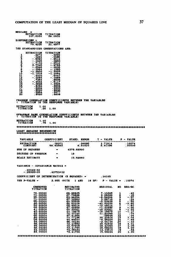
The output file corresponding to this example is printed below, and is followed by a discussion of the results in Section 3. ............................................. ROBUST REGRESSIOI VITH A C 0 I F T A . r TERX. * . . . . . . . . . . . . . . . . . . . . . . . . . . . . . . . . . . . . . . . . . . .
NI[BEROFCASES- 20 " B E R OF COEFPICIEITS CIYCLUDIIO COBSTAIT TERN) .I 2 TRE BXT-IVE SEARCH VRRSIOY VILL BE USED. DATA SET PILOT-PLAlT DATA SET VITH 0.E LEVERAGE POIIT
THE- ARE RO NISSIYG VALUES. LARGE OUTPUT IS VAITED.
THE OB8BRVATIO.S ARE:
1 2 3 4 5 6 7 6 9 10 11 12 13 14 15 16 17 18 19 20
62.0000 104.0000 57.0000 370.0000 44.0000 100.0000 16.0000 28.0000 138.0000 10s. 0000 159.0000 7s. 0000 88.0000 164.0000 169.0000 167.0000 140.0000 167.0000
TI
1
1
1
1 1
PIlof-PLm DATA SET VITH 0.8 LEVERAGE WIIT
I I-+ ---- + ---- +----+ ---- + ---- + ---- +----+ ---- + ---- + ---- +- I I I I I I I 1 I I 1 I + I I
I I
1 I I I I I 1 I I I I I I I I I I I I I 1 I I I I I 1 I
I I I 11 I I I I I I 1 I I I I 1 1 1 I I I I 1 I I I I I
.4100E+02 + 1 + I I x-+----+----+----+----+----+----+----+----+----+----+-x
.1600E+02 .3?008+03
.8000E+02 + 23
+
I
+
+
+
OBSERVED BXTRACTIOI
COMPUTATION OF THE LEAST MEDIAN OF SQUARES LINE 37
NEDIAIS - EXTRACTIOI TITRATIOI
107.0000 89.0000
DISPBRSIOIS - EXTRACTIOI TITRATIOI
70.4235 21.4977
THE STAIDARDIZED OESERVATIOIS ARE: TITRATIOI
.3256
. O M 5 -. 6512
.0930 -. 6512 - .9768 -. 8838 -. 1395 -1.3025 -1.2094
.6047 -. 0465
.a838 -.5117 - .2326
.8838 ,9303
I .8838 .6977
I .8838
PEARS01 CORRELATIOI COBPPICIBITS BBTYBEI THE VARIABLES C TITRATIOI IS THE RBswllw VARIABLE) EITRACTIOI 1.00 TITRATIOI .38 1.00
GPBARUI R A S CORRELATIOI COEFPICIBITS BBTVBBI THE VARIABLES < TITRATIOXI IS THE RBSWISJJ VARIABLE) BITRACTIOI 1.00
. . . . . . . . . . . . . . . . . . . . . . . . . . . . . . . . . . . . . . . . . . . . . . . . . . . . . . . . . . . . . . . . . . . . . . . . . . . . . . LEAST SQUARES R B G W I O X I ........................
TITRATIOI .76 1.00
VARIABLE COBFFICIEII STAID. ERROR T - VALUE P - VALUE EXTRACTIOI .08071 ,04695 1.71914 .lo274
COISTAIT 58.93883 6.61420 8.91096 . 00000
......................................................................
SVX OF SQUARES I 4379.69300
DEGREES OF FRXEDOX = 18
SCALE ESTIMTE I 15.59860
VARIAICE - COVARIABCE MTRIX = .22040-02 - .2638Dt00 .4375D+02
COEFFICIBIT OF DETERNIIIATIOII (R SQUARED) - .14103
TEE F-VALUE 2.955 WITH 1 A I D 18 DF) P - VALUE = .lo274
OBSERVED TI TRATI 01 76.00000 70.00000 55.00000 71.00000 55.00000 48.00000 50.00000 66.00000 41.00000 43.00000 82.00000 68.00000 88.00000 58.00000 64.00000 88.00000 89.00000 88.00000 84.00000 88.00000
ESTIUTED T ITRAT I01
RESIDUAL m RES/SC
7.13365 2.26362
-8.94294 3.86718
-8.53938 -40.80209 -12.49014
-1.00998 -19.23021 -18.19875
11.92298 .58646
16.22804 -6.99220 -2.04144 15.82448 16.42092 15.58234 13.03516 IS. 58234
8 9
10 11 12 13 14 .15 16 17 18 19 20
.40
. I S -. 57
.24 -.55
-2.62 -. 80 -. 06 -1.23 -1.17
.76
.04 1.04 -.45 -. 13 1.01 1.05 1.00
. 84 1.00
. . . . . . . . . . . . . . . . . . . . . . . . . . . . . . . . . . . . . . . . . . . . . . . . . . . . . . . . . . . . . . . . . . . . . . . . . . . . . .

38 SIMPLE REGRESSION
LEAST KBDIAY OF SQUARES REGRBS8IOl ...................................
OBSERVED ESTIlUTED RESIDUAL .O REWSC T I TRATI OK TITRAT 10.
1.00000 -. 60000 - .a2857 1.97144 .74286
.104.62860 -. 17143 -1.77142 -.37143 -2.14286 2.28572 -1.34285 1.68571 -1.91428 . 00000
, 11429 -.45714 - .a2857 .a2850 - .a2857
1 .75 2 -.45 3 -.62 4 1.48 5 .56 6 -78.50 7 -.13 8 -1.33 9 -.28 10 -1.61 11 1.71 12 -1.01 13 2.26 14 -1.44
1 15 .OO I 16 .09
17 -.34 18 -.62
I 19 .62 20 -.62
*************************%**************************************************%* REVEIGHTED LEAST SQUARES BASED OH THE L B . . . . . . . . . . . . . . . . . . . . . . . . . . . . . . . . . . . . . . . . . . . .
VARIABLE COEFFICIEllT STAXD. ERROR T - VALUE P - VALUE EXTRACT Ion .32261 .00595 54.21467 .ooooo COIISTAUT 35.31744 .69617 50.73091 . 00000
......................................................................
WEIGHTED SUII OF SQUARES - 26.75224 DEGREES OF FREEDOX = 17
SCALE ESTXIUTE I 1.25446
VARIAXE - COVARIAUCE X&TRIX - .3541D-O4 - ,37723)-02 .4847D+OO
COEFFICIEFT OF DETERllIUATIOII CR SQUARED) - .99425
THE F-VALUE = 2939.231 CVITH 1 A I D 17 DF) P - VALUE = .OOOOO
THERE ARE 19 WIXTS VITH KOU-ZERO "EIGHT. AVERAGE VEIGHT - .95000
OBSERVED ESTIIUTED RESIDUAL XO REWSC YBIGIiT TITRATIOB T ITRAT IOII
1.00116 - .482221 -. 319421 2.13081 1.29362
-106.66420 .48759 - 1.57874 .52075
-1.35061 2.16197 -1.19180 1.38710 -1.5 1341 .29262 - .22597 -. 83904
-1.19380 .el323
-1.19360
9 10 11 12 13 14 15 16 17 18 19 20
. 60 -.38 -.25 1.70 1. 03
-85.04 .39
-1.26 .42
-1.08 1.72 -.95 1.11
-1.21 .23 -. 18 -. 67 -. 95 .4* -. 95
1.0 1.0 1.0 1.0 1.0
. o 1.0 1.0 1.0 1.0 1.0 1.0 1.0 1.0 1.0 1.0 1.0 1.0 1.0 1.0

INTERPRETATION OF THE RESULTS 39
3. INTERPRETATION OF' THE RESULTS
The output provided by PROGRESS starts with some general informa- tion about the data set. In the above example, the data were two- dimensional so they could be plotted. A point in the scattergram is represented by a digit. This digit corresponds to the number of points having approximately the same coordinates. When more than nine points coincide, an asterisk (*) is printed in that position. In simple regression, such a plot reveals immediately which points may exert a strong influence on the LS estimates.
The program then prints the median mi of each variable j. In the Pilot-Plant output displayed above, the median extraction value is 107 and the median titration value equals 69. On the next line, the dispersion sj of each variable is given, which can be considered as a robust version of its standard deviation (the exact definition will be given in Section 1 of Chapter 4). When large output has been requested, the program then provides a list of the standardized observations, in which each measure- ment xii is replaced by
xii - mj ' i
(the response variable is standardized in the same way). The columns of the resulting table each have a median of 0 and a dispersion of 1. This enables us to identify outliers in any single variable. Indeed, if the absolute value of a standardized observation is large (say, larger than 2.5) then it is an outlier for that particular variable. In the Pilot-Plant output we discover in this way that case 6 has an unusually large extraction measurement, because its standardized value is 3.73. (Sometimes the standardized values can tell us that the distribution in a column is skewed, thereby suggesting data transformation.) The standardization is per- formed differently when there is no constant term in the regression, as we shall see in Section 6.
Next, PROGRESS provides the Pearson (product-moment) correla- tion coefficients between the variables, as well as the nonparametric Spearman correlation coefficients.
Before giving the robust estimates, PROGRESS starts with the classi- cal LS results. A table is printed with the estimated coefficients, along with their standard error. The standard error of the jth LS regression coefficient is the square root of the jth diagonal element of 'the variance- covariance matrix of the LS regression coefficients, given by a2(XrX)-',

40 SIMPLE REGRESSION
where the matrix X is given by
...
...
...
The ith row of X equals the vector xi consistin of the p explanatory variables of the ith observation. The unknown cr is estimated by !
where ri = yi - f i is the ith residual. The estimated variance-covariance matrix s2(X'X)-' is also contained in the output. (Because this matrix is symmetric, only its lower triangular part is given, including the main diagonal.) For simple regression, p = 1 when there is no intercept term, and p = 2 otherwise. In the output, the quantity indicated by SCALE
To construct confidence intervals for the parameters 9, one has to assume that the errors e, are independently normally distributed with mean zero and variance t~*. Under these conditions, it is well known that each of the quantities
ESTIMATE is s = V7.
A 9-3 j = 1 , . . . , p v q ' (3.3)
has a Student distribution with n - p degrees of freedom. Let us denote the 1- a / 2 quantile of this distribution by tn-p,l-a,2. Then a (1 - a) x 100% confidence interval for 9 is given by
for each j = 1, . . . , p. The same result can also be used for testing the significance of any regression coefficient, such as 4. The hypotheses are
(3.5) H,: f$ = 0 (null hypothesis) Hl : 62. # 0 (alternative hypothesis) .

INTERPRETATION OF THE RESULTS 41
Such a test may be helpful in determining if the jth variable might be deleted from the model. If the null hypothesis in (3.5) is accepted (for a certain value of a), then this indicates that the jth explanatory variable does not contribute much to the explanation of the response variable. The test statistic for this hypothesis is
This ratio corresponds to “T-VALUE’ in the output of PROGRESS. The null hypothesis will be rejected at the level a when the absolute value of “T-VALUE’ is larger than tn-p,l-p,z (in this case we will say that the jth regression coefficient is significantly different from zero).
In the present example, n = 20 and p = 2. The 97.5% quantile (since we use a = 5%) of the Student distribution with n - p = 18 degrees of freedom equals 2.101. Therefore, one can conclude that the LS slope is not significantly different from zero, because its associated t-value equals 1.719. On the other hand, the intercept t-value equals 8.911, which is quite significant.
Next to each t-value, PROGRESS also prints the corresponding (two-sided) “p-value” or “significance level.” This is the probability that a Student-distributed random variable with n - p degrees of freedom becomes larger in absolute value than the t-value that was actually obtained. In order to compute this probability, we used the exact formulas of Lackritz (1984) as they were implemented by van Soest and van Zomeren (1986, personal communication). When the p-value is smaller than 0.05, then the corresponding regression coefficient is signific- ant at the 5% level. In the above output, the p-value of the LS slope equals 0.10274 so it is not significant, whereas the p-value of the LS intercept is given as 0.00000, which makes it significant (even at the 0.1% level). The printed p-values make hypothesis testing very easy, because probability tables are no longer necessary.
However, (3.6) has to be used with caution because it is not robust at all. The distribution theory of this statistic only holds when the errors really follow a Gaussian distribution, which is rarely fulfilled in practice. It is therefore advisable to look first at the robust fit in order to be aware of the possible presence of outliers. In Section 4, we will give some guidelines based on the residuals resulting from the robust fit for identify- ing the harmful observations. When it appears that the data set contains influential points, then one has to resort to the t-values of the RLS solution, which will be presented below.

42 SIMPLE REGRESSION
In order to obtain an idea of the strength of the linear relationship between the response variable and the explanatory variable(s), the coef- ficient of determination (R') is displayed in the output. R2 measures the proportion of total variability explained by the regression. For the exact formula one has to distinguish between regression with and without a constant term. For LS regression, RZ can be calculated as
in the model without constant term SSE SST
R Z = l - -
and as
in the model with constant term, SSE SST,
R Z = l - -
where
SSE = residual error sum of squares n
= i: ( y i -jg, i = l
SST = total sum of squares
and
SST, = total sum of squares corrected for the mean
where
In the case of simple regression with constant term, the coefficient of determination equals the square of the Pearson correlation coefficient between x and y, which explains the notation R'.
For the Pilot-Plant data (with outlier), the R2 value corresponding to LS equals 0.141. This means that only 14.1% of the variability in y is explained by the simple regression model.

INTERPRETATION OF THE RESULTS 43
One can also consider testing the hypothesis that R2 equals zero. Formally,
(3.7) H,: R2 = 0 (null hypothesis) H,: R2 # 0 (alternative hypothesis) .
These hypotheses are equivalent to testing whether the whole vector of regression coefficients (except for the constant term if the model has one) equals the zero vector, that is, (3.7) is equivalent to
(3.8) H,: All nonintercept 9's are together equal to zero H,: Ho is not true.
This is quite different from the above t-test on an individual regression coefficient, because here the coefficients are considered together. If the ei are normally distributed, then the following statistics have an F- distribution:
(SST, - SSE)/( p - 1) SSE/(n - p) - Fp-1."-p
R2/(p-1) - - (1 - R 2 ) / ( n - p )
for regression with a constant, and
otherwise. R 'Ip - - (SST - SSE) l p
(1 - R 2 ) / ( n - p) SSEI(n - p) FP*n-P
If the calculated value of the appropriate statistic is less than the (1- a)th quantile of the associated F-distribution, then H, can be accepted. If not, H, may be rejected. To facilitate this test, PROGRESS prints the p-value of the F-statistic. This p-value (again computed accord- ing to Lackritz 1984) is the probability that an F-distributed random variable with the proper degrees of freedom exceeds the actual F-value.
For the contaminated Pilot-Plant data we obtain an F-value of 2.955, with 1 and 18 degrees of freedom. The corresponding p-value is 0.103, so we have no significance at the 5% level. Consequently, one can say that it appears from the LS estimates that the explanatory variable does not really "explain" the response in a significant way, since one cannot reject
The interpretation of t-test, R2, and F-test is still valid for the multidimensional data sets that will be considered in Chapter 3.
When intermediate or large output is requested, the program con- tinues by listing, for each observation, the actual value of the response
HO.

44 SIMPLE REGRESSION
( y i ) , the estimated response ( yl i ) , the residual (ri = yi - f i ) , and the standardized residual (ri /s) . This table allows us to identify outlying residuals. However, because case 6 has attracted the LS line so strongly (see Figure 2), and has also blown up s, its standardized residual is merely -2.62, which is perhaps slightly conspicuous but in no way dramatic.
The results for LMS regression are printed below the output for LS. First the estimates of the regression parameters are given, together with a corresponding scale estimate. This scale estimate is also defined in a robust way. For that purpose a preliminary scale estimate so is calculated, based on the value of the objective function, multiplied by a finite sample correction factor dependent on n and p:
so = 1.4826(1+ -&-) JmedrT .
With this scale estimate, the standardized residuals ri/so are computed and used to determine a weight wi for the ith observation as follows:
1 if Iri/sol 5 2.5 0 otherwise.
wi =
The scale estimate for the LMS regression is then given by
(3.9)
(3.10)
Note that u* also has a 50% breakdown point, which means that it does not explode (u*-- ,m) or implode (u*+O) for less than 50% of contami- nation. More details on this scale estimate will be given in Chapter 5 . In the present example, u* = 1.33, which is much smaller than the LS scale s = 15.6 computed in the beginning.
The LMS also possesses a measure to determine how well the fitted model explains the observed variability in y. In analogy to the classical one, we called it also RZ or coefficient of determination. In the case of regression with constant term, it is defined by
(3.11)

INTERPRETATION OF THE RESULTS
and by
45
(3.12)
when the model has no intercept term. Here, the abbreviation “mad” stands for median absolute deviation, defined as
mad ( Y i ) = med {I Yi - m ~ d Yj I I *
Independent of our work, formula (3.11) was also proposed by Kvalseth (1985). In the Pilot-Plant output the robust coefficient of determination equals 0.996, which means that the majority of the data fits a linear model quite nicely.
Also for the LMS, a table with observed y i , estimated Y i , residual ri , and standardized residual ri/u* is given. It now shows clearly that case 6 is an outlier, because r6/u* equals the enormous value of -78.50.
The last part of the output is about reweighted least squares (RLS) regression. This corresponds to minimizing the sum of the squared residuals multiplied by a weight wi:
n
MiniFize E w i r t . (3.13) @ i - 1
The weights wi are determined from the LMS solution as in (3.9), but with the final scale estimate u* (3.10) instead of so. The effect of the weights, which can only take the values 0 or 1, is the same as deleting the cases for which wi equals zero. The scale estimate associated with (3.13) is given by
C. wir? s = i = l
I n (3.14)
(One finds again the scale estimate for ordinary LS when putting wi = 1 for all cases.) Therefore, the RLS can be seen as ordinary LS on a “reduced” data set, consisting of only those observations that received a nonzero weight. Because this reduced data set does not contain regres- sion outliers anymore, the statistics and inferences are more trustworthy than those associated with LS on the whole data set. The underlying

46 SIMPLE REGRESSION
distribution theory is no longer entirely exact (because the weights depend on the data in a complicated way), but is still useful as a good approximation, as was confirmed by means of some Monte Car10 trials.
In the present example all wi are equal to 1, except for case 6, which indeed was the outlier we had produced. The regression coefficients obtained by RLS strongly resemble those determined in the first step by LMS. Note that, without the outlier, the slope estimate becomes signific- antly different from zero.
The determination coefficient for the RLS is defined in an analogous way as for LS, but all terms are now multiplied by their weight wi. In this example it is highly significant, because the F-value becomes very large and hence the corresponding p-value is close to zero. To end this section, we would like to warn the reader about a common
misunderstanding. When the LS and the RLS results are substantially different, the right thing to do is to identify the outliers (by means of the RLS residuals) and to study them. Instead, some people are inclined to think they have to choose between the LS and the RLS output, and typically they will prefer the estimates with the most significant r-values or F-value, often assuming that the highest R2 corresponds to the “best” regression. This makes no sense, because the LS inference is very sensitive to outliers, which may affect R2 in both directions. Indeed, the least squares R2 of any data set can be made arbitrarily close to 1 by means of a sequential approach to detect outliers via stepwise deletion. the outliers that were responsible for a high R“ and correctly comes to the conclusion that the R2 of the majority is not so high at all (or it may find that some t$ are no longer significantly different from zero).
4. EXAMPLES
In this section we will further explain the results provided by PROGRESS, by means of some real-data examples appearing in the literature.
Example 1:
This two-dimensional data set comes from Mickey et al. (1967) and has been widely cited. The explanatory variable is the age (in months) at which a child utters its first word, and the response variable is its Gesell adaptive score. These data (for 21 children) appear in Table 4, and they are plotted in Figure 5 .
Mickey et al, (1967) decided that observation 19 is an outlier, by means of a sequential approach to detect outliers via stepwise regression. Andrews and Pregibon (1978), Draper and John (1981), and Paul (1983)
First Word-GeseU Adaptive Score Data

Table 4. First Word-Gesell Adaptive Score Data
Child Age in Months Gesell Score (i) (xi ) (Yi) 1 2 3 4 5 6 7 8 9
10 11 12 13 14 15 16 17 18 19 20 21
15 26 10 9
15 20 18 11 8
20 7 9
10 11 11 10 12 42 17 11 10
95 71 83 91
102 87 93
100 104 94
113 96 83 84
102 100 105 57
121 86
100
Source: Mickey et al. (1967).
.- 9 c, P (D 'p (D
Figure
P 1 I I I I I I 1 1 I I ) I I I I ( I 4 - - -
0 - - 19 120 - - - - - - - - - - - - - -
60 - - - - I I I I I I I I I I I I I I I I
- 10 20 30 40
Age at first word (months) 5. Scatterplot of Gesell adaptive score versus age at first word.
47

48 SIMPLE REGRESSION
applied outlier diagnostics to this data set. (The use of such diagnostics will be discussed in Chapter 6.) The most important results of our own analysis are given below.
AGE CIODSTH) -1.12699 .31017 -3.63343 COXSTAFT 109.87380 5.06780 21.68077
SUU OF SQUARES I 2308.58600
DECREES OF PREEWN L 19
SCALE BGTIMTE L 11.02291
VARIMCE - COVARINCE NATRIX .9621D-01 -. 1384Dt01 .2568D+02
WEFPICIEST OF DETERNISATIOB (R SQUARED) = .40997
THE P-VALW - 13.202 WITH 1 A I D 19 DF) P - VALUE OBSERVED ESTIIUTED RESIDUAL SO
GBGELL SC. GESELL sc. 95.00000 71.00000 83.00000 91.00000 102.00000 87.00000 93.00000 100.00000 104.00000 94.00000 113.00000 96.00000 83.00000 84.00000 102.00000 100.00000 105.00000 57.00000 121.00000 86.00000 100.00000
92.96901 80.57213 98.60395 99.73094 92.96901 67.33406 89.58804 97.47696 100.85790 87.33406 101.98490 99.73094 98.60395 97.47696 97.47696 98.60395 96.34998 62.54031 90.71503 97.47696 98.60395
.00177
.ooooo
.00177
PEWSC
. 18 -. 87 -1.42 -. 79 .82 -. 03 .31 .23 .29 .60 1.00 - .34 -1.42 -1.22 .41 .13 .78
- .50 2.75 -1.04 .13
VARIABLE WEPPICIEST ACE <NOSTH> -1.50000
WSSTAIT 119.75000
..............................
FIBAL SCALE ESTINATE - 8.83928
COEFFICIEYT OF DETERNIBATIOS - .44460
OBSERVED GBSBLL SC. 95. 00000 71.00000 83.00000 91.00000 102.00000 87.00000 93.00000 100.00000 104.00000 94.00000 113.00000 96.00000 83.00000 84.00000 102.00000 100.00000 105.00000 57.00000 121.00000 86.00000 100.00000
S T I X A T E D CBWLL sc. 97.25000 80.75000 104.75000 106.25000 97.25000 69.75000 92.75000 103.25000 107.75000 89.75000 109.25000 106.25000 104.75000 103.25000 103.25000 104.75000 101.75000 56.75000 94.2SOOO 103.25000 104.75000
RESIDUAL YO RBS/SC
-2.25000 -9.75000 -21.75000 -15.25000 4.75000 -2.75000
.25000 -3.25000 -3.75000 4.25000 3.75000
-10.25000 -21.75000 -19.25000 -1.25000 -4.75000 3.25000
.25000 26.75000 -17.25000 -4.75000
1 2 3 4 5 6 7 8 9 10 11 12 13 14 15 16 17 18 19 20 21
-.25 -1.10 -2.46 -1.73 .54 -. 31 .03 -. 37 -. 42 .48 .42
-1.16 -2.46 -2.18 -. 14
-.54 .37 .03 3.03 -1.95 -. 54

EXAMPLES 49
REVBIGHTED LEAST SQUARES BASED OU THE LXS ......................................... VAR I ABLE COEFPICIEUT S T A I D . ERROR T - VALUE P - VALUE AGE(U0ETH) -1.19331 .2434a -4,90100 .00012
COUSTAXT 109.30470 3.96997 27.53290 . 00000
......................................................................
WEIGHTED SUX OF SQUARES = 1340.02400
DEGREES OF FREEWX - i a SCALE ESTIMATE = 8.62820
VARIMCE - COVARIANCE NATRIX .5928D-01
- . ~ ~ ~ B D + o o .157833+02
COEFFICIEUT OF DETERNIWATIOE (R SQUARED) = .57163
THE F-VALUE = 24.020 WITH i AUD i a DF) P - VALUE - .00012
THERE ARE 20 WIXTS WITH EOB-ZERO VEIGHT. AVERAGE WIGHT I .9523a
OBSERVED GESELL SC.
95.00000 71.00000 83. ooooo 91.00000
102.00000 87. ooooo 93.00000
100.00000 104.00000 94.00000
113.00000 96.00000
102.00000 100.00000 105.00000 57.00000
121.00000
100.00000
a3. ooooo 84. ooooo
86. ooooo
ESTINATED GHSBLL SC.
RESIDUAL
3.59498
-14.37157 -7.27860
-7.50ma 10.59498 1.50151
4 .24 ia i a.56154
12.04~19 -2 .5aaa
-12.17a26 5.azi72 2 . 0 2 ~ 3
-2.10563 31.9amo
-10. 17826 2. a2843
5.17491 3.82174
- 14.37 157
10.01505
EO RES/SCVElGXl
1 2 s 4 5 6 7
9 10 11 12 13 14 15
a
:$ i a 19 20 21
.42
-1.67 -.a8 1.23
.44
.49 I99
1.40 - .30
-1.67 -1.41
.67
.30 1.16 - .25 3.71
.30
-.a4
. ia . ao
-1. ia
1 . 0 1 .0 1 .0 1 .0 1 . 0 1 .0 1 .0 1 .0 1 . 0 1 . 0 1 . 0 1 .0 1 . 0 1 .0 1 . 0 1 . 0 1 . 0 1 .0
. o 1 . 0 1 . 0
Because medium-sized output was requested, PROGRESS gives for each estimator a table with the observed response variable ( y i ) , its estimated value ( F i ) , the residual (ri), and the standardized residual (denoted by “RES I SC”) . The standardized residuals for each regression are obtained by dividing the raw residuals by the scale estimate of the fit. A supplementary column with weights is added to the table for RLS regression. (These weights are determined from the LMS solution, as described in Section 3.) In this example, the case with index 19 received a zero weight. Indeed, this case has been identified as outlying because it has a large residual from the LMS fit. The equations of the LS and the RLS do not differ very much for this data set. The pair of points 2 and 18 has pulled the LS in the “good” direction. These points are good leverage points and possess small LMS residuals as well as small LS residuals. (The deletion of one or both of these points would have a considerable effect on the size of the confidence intervals.) One might even say that this data set is not a very good example of linear regression because deleting the leverage points (2 and 18) would not leave much of a linear

50 SIMPLE REGRESSION
relationship between x and y. (We will return to this at the end of Section 6.)
Example 2:
This data set (listed in Table 5 ) shows the trend from 1976 to 1980 of the number of reported claims of Belgian fire-insurance companies (from the annual report of the Belgian Association of Insurance Companies). It is included here to have an example with very few points.
When looking at the scatterplot in Figure 6, one notices a slight upward trend over the years. However, the number for 1976 is extraordi- narily high. The reason lies in the fact that in that year the summer was extremely hot and dry (compared to Belgian standards), causing trees and
Number of Fires in 1976-1980
Table 5. Number of Fire Claims in Belgium from 1976 to 1980
Year Number of fires ( X i 1 ( Y i )
76 16,694 77 12,271 78 12,904 79 14,036 80 13,874
16.000 F----l - -
-
76 77 78 79 80 Year
Figure 6. Number of fire claims in Belgium for the years 1976-1980.

EXAMPLES 51
bushes to catch fire spontaneously. It is striking that the LS y ^ = -387.5~ + 44180.8 (dashed line) and the LMS y^ = 534.3~ - 28823.3 (solid line) are very different. The LS fits the data with a decreasing trend, whereas the LMS line increases. The outlier lies on the outside of the x-range and causes LS to grossly misbehave. It does not even possess the largest LS residual. This example shows again that examination of the LS residuals is not sufficient to identify the outlier(s).
Of course, in such a small data set one cannot draw any strong statistical conclusions, but it does show that one should think carefully about the data whenever LS and LMS yield substantially different results.
Example 3: Annual Rates of Growth of Prices in China
Table 6 contains the annual rates of growth of the average prices in the main cities of Free China from 1940 to 1948 (Simkin 1978). For instance, in 1940 prices went up 1.62% as compared to the previous year. In 1948 a huge jump occurred as a result of enormous government spending, the budget deficit, and the war, leading to what is called hyperinflation.
The LMS regression equation is given by
y = 0.102~ - 2.468 ,
whereas the LS estimate corresponds to
y^ = 24.845~ - 1049.468 ,
Table 6. Annual Rates of Growth of Average Prices in the Main Cities of Free China from 1940 to 1948
Year Growth of Prices Estimated Growth (xi 1 ( Y i ) By LMS By LS
40 1.62 1.61 -55.67 41 1.63 1.71 -30.82 42 1.90 1.82 -5.98 43 2.64 1.92 18.87 44 2.05 2.02 43.71 45 2.13 2.12 68.56 46 1.94 2.22 93.40 47 15.50 2.33 118.25 48 364.00 2.43 143.09
Source: Simkin (1978).

52 SIMPLE REGRESSION
which is totally different. To show which of these lines yields the better fit, Table 6 lists the estimated values by both methods. The LMS provides a fair approximation to the majority of the data, except of course for the last two years, where the observed yi go astray. On the other hand, the LS fit is bad everywhere: The estimated Yi is even negative for the first three years, after which it becomes much too large, except for the 1948 value, which it cannot match either. Least squares smears out the effect (of nonlinearity of the original data) over the whole column, whereas LMS fits the majority of the data (where it is indeed linear) and allows the discrepancy to show up in those two years where actually something went wrong. Applying PROGRESS to this data set yields (among other things) the following output:
B U W B J 3 R O F C A S E S - B IIIHEER OF COEFFICIEFTS <IllCLUDIllG COBSTAET TERM) 2
THE EXTEBSIVE SEARCH VERSIOB VILL BE USED. DATA SET AXIUAL RATES OF GROWA OF PRICES I B CAIEA THERE ARE IID M I S I B G VALUES.
A X I U A L RATES OF GROWH OF PRICES I l l CAIBA
OBSERVED PRICEGROW
.3640E+03
+ + I I 1 I I 1 I I t t I I I I I I I I
1 I I I I I I I t + I I I I I I I I t t 1 I I I I I I I
I I I 1 I
1 1 1 1 1 I I I
.1620E+01 + 1 1 + I I I-+----+----+----+----+----+----+-----+----+----+----+----t-I
.4000B+O2 .4800Et02
OBSERVED YEAR
+ +
+

EXAMPLES 53
=DIMS = YEAR PRICEGROVT
44.0000 2.0500
DISPERSIOW = YEAR PRICEGROVT
2.9652 .6227
THE STAEDARDIZED OBSRRVATIOIS ARE: YEAR PRICEGROVT
1 -1.3490 -.4906 2 -1.0117 -.6?45 3 -.6745 -.2409 4 - .33?2 .9475 5 . 0000 . 0000 6 .3372 .1285 7 .674?i -.1767 8 1.0117 21.5998 9 1.3490 581.2665
PH-I CORRELATIOI COBFFICIH.rs BETVEEI THE VARIABLES ( PRICEGROVT IS THE RESPOISE VARIABLE)
YEAR 1.00 PRICEGROVT .57 1.00
SPEARMI RAEK CORRELATIOI COEFFICIEETS BETVEE. THE VARIABLES < PRICEGROVT IS THE RESPOSSZ VARIABLE)
YEAR 1.00 PRICEGROVT .85 1.00
************************************************************%***%*************
LEAST sQUARES RECRBGSIOY *********a**************
VARIASCE - COVARIMCE HATRIX =
.1870D+03 -. 8227D+04 .3632D+06
COEFFICIEFT OF DETERMISATIOI <R SQUARED) = .32047
THE P-VALUE = 3.301 WITH 1 ABD 7 DF) P - VALUE .11207
ORSBRVED PRICEGROVT
1.62000 1.63000 1.90000 2.44000 2.05000 2.13000 1.94000 15.50000 364.00000
ESTIMTED PR I CEGROVT -55.66766 -30.82269 -5.97766 18.86731 43.71228 68.55737 93.40234 118.24730 143.09230
RESIDUAL m RWSC
57 .28766 32.45269 7.87766
-16.22731 -41.66228 -64.42738 -91.44234 -102.74730 220.90770
8 9
.54
.31 . 07 -. 15 -. 39 -. 63 -. 86 -. 97 2.09

54 SIMPLE REGRESSION
VARIABLE COEFPICIEYT YEAR .lo200
COSSTAIT -2.46800
_______________-_-_-----------
FIIAL SCALE ESTIlUTE - .15475
COEFFICIEBT OF DETERNIYATIOY - .93824
RESIDUAL I0 REG/%
1.62000 1.61200 .00800 1 .05 -.08400 2 -.54 .08400 3 .54 1.63000 1.71400 .72200 4 4.67
1.90000 1.81600 .03000 5 .I9 2.64000 1.91800
2.02000 .00800 6 .05
2.05000 2.13000 2.12200 -.28400 7 -1.84
13.17400 8 85.13 1.04000 2.22400 361.57200 9 2338.42
15.50000 2.32600 364.00000 2.42800

EXAMPLES 55
Note that observations 8 and 9 are outliers in the y-direction, which show up in the second column of the standardized data. Also, the Spearman rank correlation is much higher than the Pearson correlation because the outliers have disturbed the linear relation, whereas they obey the near-monotone relation between both variables.
For this example, we will discuss the residual plots (printed above) provided by PROGRESS. They display the standardized residual versus the estimated value of the response. An index plot is similar, except it contains the standardized residual plotted versus the index of the observa- tion. (This makes it easier to find which observation corresponds to a given point in the plot. The index plot is also useful because the indices often reflect the order in which the observations were measured, so it may reveal sudden changes in the data recording process.) In both plots, a dashed line is drawn through zero, and a horizontal band on the interval [-2.5,2.5] is marked. These lines facilitate the interpretation of the

56 SIMPLE REGRESSION
results. When the observed value yi equals the estimated value pi, then the resulting residual becomes zero. Points in the neighborhood of this zero line are best fitted by the model. If the residuals are normally distributed, then one can expect that roughly 98% of the standardized residuals will lie in the interval [-2.5,2.5]. Thus, observations for which the standardized residuals are situated far from the horizontal band can be identified as outlying.
The first residual plot in the above output shows how the LS fit masks the bad point. The LS has been pulled away by this outlier, and its scale estimate has exploded. The LS residual associated with the outlier even lies within the horizontal band. Because of this effect, the interpretation of a residual plot corresponding to the LS estimator is dangerous. In the residual plot of the LMS, the outlier is very far away from the band. Residual plots corresponding to robust estimators are even more useful in problems with several variables, as will be illustrated in Chapter 3.
These graphical tools are very convenient for spotting the outlying observations. The LS result can be trusted only if the residual plots of both the robust and nonrobust regression methods agree closely.
Besides the identification of outliers, the residual plot provides a diagnostic tool for assessing the adequacy of the fit and for suggesting transformations. An ideal pattern of the residual plot, which indicates an adequate model and well-behaved data, is a horizontal cloud of points with constant vertical scatter. Anomalies in the pattern of residuals can lead to several courses of action. For instance, the plot may indicate that the variance of the residuals increases or decreases with increasing estimated y or with another variable. (See the education expenditure data in Section 3 of Chapter 3 for an illustration.) This is called heteroscedas- ticity, in contrast to the classical model where the errors have a constant variance, in which case we speak of homoscedasticity. This problem may be approached by applying a suitable transformation on either an ex- planatory or the response variable. If this heteroscedasticity appears in an index plot, then one should turn back to the origin of the data in order to look for the cause of the phenomenon. For example, it could be that a time-related variable has to be included in the model.-Also, other model failures may be visible in residual plots. A pattern resembling a horseshoe may be caused by nonlinearity. (See the cloud point data in Section 3 of Chapter 3 for an example.) In such a situation, a transformation on an explanatory or on the response variable, or an additional squared term or a cross-product term in the model, or the addition of an extra explanatory variable may be required. (In many applications of regression, there is a substantial amount of prior knowledge that can be useful in choosing between these possibilities.)

EXAMPLES 57
Exampkk 4: Brain and Weight Dah Table 7 presents the brain weight (in grams) and the body weight (in kilograms) of 28 animals. (This sample was taken from larger data sets in Weisberg 1980 and Jerison 1973.) It is to be investigated whether a larger brain is required to govern a heavier body.
A clear picture of the relationship between the logarithms (to the base 10) of these measurements is shown in Figure 7. This logarithmic
Table 7. Body and Brain Weight for 28 Animals
Index Body Weight" Brain Weightb
1 2 3 4 5 6 7 8 9 10 11 12 13 14 15 16 17 18 19 20 21 22 23 24 25 26 27
Mountain beaver cow Gray wolf Goat Guinea pig Diplodocus Asian elephant Donkey Horse Potar monkey Cat Giraffe Gorilla Human African elephant Triceratops Rhesus monkey Kangaroo Hamster Mouse Rabbit Sheep Jaguar Chimpanzee Brachiosaurus Rat Mole
1.350 465.000 36.330 27.660 1.040
11700.000 2547.000 187.100 521.000 10.000 3.300
529.000 207.000 62.000
6654.000 9400.000
6.800 35.000 0.120 0.023 2.500 55.500 100.000 52.160
87000.000 0.280 0.122
8.100 423.000 119.500 115.000 5.500 50.000
4603.000 419.000 655.000 115.000 25.600 680.000 406.000 1320.000 5712.000 70.000 179.000 56.000 1 .Ooo 0.400 12.100 175.000 157.000 44o.Ooo 154.500 1.900 3.000
28 Pig 192.000 180.000
'In kilograms. *In grams. Source: Weisberg (1980) and Jerison (1973).

58 SIMPLE REGRESSION
- 4.0 -
-
E
3 c 2.0 E n 3
M Q, .-
- .-
1 - - - -
- - , 1 1 1 1 I I I I I I I I 1 I I I m
0.0 2.0 4.0 Log body weight
F i i 7. Logarithmic brain weight versus logarithmic body weight for 28 animals with LS (dashed line) and RLS fit (solid line).
transformation was necessary because plotting the original measurements would fail to represent either the smaller or the larger measurements. Indeed, both original variables range over several orders of magnitude. A linear fit to this transformed data would be equivalent to a relationship of the form
between brain weight (y) and body weight (x). Looking at Figure 7, it seems that this transformation makes things more linear. Another impor- tant advantage of the log scale is that the heteroscedasticity disappears.
The LS fit is given by
log 9 = 0.49601 log x + 1.10957
(dashed line in Figure 7). The standard error associated with the slope equals 0.0782, and that of the intercept term is 0.1794. In Section 3, we explained how to construct a confidence interval for the unknown regres- sion parameters. For the present example, n = 28 and p = 2, so one has to

EXAMPLES 59
use the 97.5% quantile of the t-distribution with 26 degrees of freedom, which equals 2.0555. Using the LS results, a 95% confidence interval for the slope is given by t0.3353; 0.65673. The RLS yields the solid line in Figure 7, which is a fit with a steeper slope:
log j? = 0.75092 log n + 0.86914 . The slope estimated by the RLS technique even falls outside the 95% confidence interval associated with the LS fit! The standard error of the regression coefficients in RLS is reduced remarkably as compared with
Table 8. Standardized LS and RLS Residuals for the Brain and Body Weight Data
Standardized LS Standardized RLS Index Species Residuals Residuals Wi
1 2 3 4 5 6 7 8 9
10 11 12 13 14 15 16 17 18 19 20 21 22 23 24 25 26 27
Mountain beaver COW Gray wolf Goat Guinea pig Diplodocus Asian elephant Donkey Horse Potar monkey cat Giraffe Gorilla Human African elephant Triceratops Rhesus monkey Kangaroo Hamster Mouse Rabbit Sheep Jaguar Chimpanzee Brachiosaurus Rat Mole
-0.40 0.29 0.29 0.36
-0.57 -2.15
1.30 0.58 0.54 0.68 0.06 0.56 0.53 1.69 1.13
-1.86 1-10
-0.19 -0.98 -1.04 -0.34
0.40 0.14 1.02
-2.06 -0.84 -0.27
-0.27 -1.13
0.17 0.50
-0.65 -10.19
1.08 0.21
-0.43 2.02 0.68
-0.37 0.00 4.15 0.08 - -9.20
3.47 - 1.29 -0.81 -0.17 -0.39
0.29 -0.80
2.22 - 10.94 -0.80
1.35
1 1 1 1 1 0 1 1 1 1 1 1 1 0 1 0 0 1 1 1 1 1 1 1 0 1 1
28 Pig 0.02 -1.50 1

60 SIMPLE REGRESSION
the LS, namely 0.0318 for the slope and 0.0618 for the constant term. A 95% confidence interval for the unknown slope is now given by [0.6848; 0.81711, which is narrower than the interval coming from LS. The f-values associated with the RLS regression coefficients are very large, which implies that the slope and intercept are si nificantly different from zero. Moreover, the determination coefficient R , which is a summary measure for overall goodness of fit, increases from 0.608 for LS to 0.964 for RLS. This example shows that not only the LS regression coefficients, but also the whole LS inference, may become doubtful in the presence of outliers.
Table 8 lists the standardized LS and RLS residuals and the w i determined on the basis of the LMS. From the RLS, it is easy to detect unusual observations and to give them special consideration. Indeed, looking at the five cases with zero w i , one can easily understand why they have to be considered as outlying. The most severe (and highly negative) RLS residuals are those of cases 6, 16, and 25, which are responsible for the low slope of the LS fit. These are three dinosaurs, each of which possessed a small brain as compared with a heavy body. In this respect they contrast with the mammals which make up the rest of the data set. The LMS regression also produced a zero weight for cases 14 and 17, namely the human and the rhesus monkey. For them, the actual brain weight is higher than that predicted by the linear model. Unlike the dinosaurs, their residuals are therefore positive. Concluding, one could say that dinosaurs, humans, and rhesus monkeys do not obey the same trend as the one followed by the majority of the data.
5
5. AN ILLUSTRATION OF THE EXACT FIT PROPERTY
The phrase “exact fit” stands for situations where a large percentage of the observations fits some linear equation exactly. For example, in simple regression this happens when the majority of the data lie exactly on a straight line. In such a case a robust regression method should recover that line. At an Oberwolfach Meeting, Donoho (1984) called this the exact fit property. For instance, the repeated median satisfies this property (Siegel 1982), a5 well as the LMS (Rousseeuw 1984). When at least n - [n/2] + 1 of the observations lie on the same line, then the equation of this line will be the LMS solution. More details on the exact fit property and its relation to the breakdown point can be found in Section 4 of Chapter 3.
The data in Table 9 come from Emerson and Hoaglin (1983, p. 139). They were devised by A. Siegel as a counterexample for the resistant line estimator (which will be briefly discussed in Section 7). Looking at the

AN ILLUSTRATION OF THE EXACX FIT PROPERTY 61
Table 9. Siegel's Data Set
i Xi Y i
1 -4 0 2 -3 0 3 -2 0 4 -1 0 5 0 0 6 1 0 7 2 -5 8 3 5 9 12 1
Source: Emerson and Hoaglin (1983).
scatterplot of these data (Figure 8), Emerson and Hoaglin suggest that a line with slope 0 would be a reasonable summary. Indeed, six out of the nine points actually lie on the line with zero slope and zero intercept. By running PROGRESS we see that least median of squares yields this line exactly, unlike least squares.
Exact fit situations also occur in real data. One example has to do with the use of an electron microscope in crystallography. Several discrete variables (such as the number of edges and certain symmetry properties) are observed for a large number of "cells" (consisting of molecules) in a
-4 -5 t 11 l i l l l l l l l l ' l l l r l ' l l
-4 -2 0 2 4 6 8 10 12
Figure 8. Example of exact fit: Scatterplot of Siegel's data set with LS (dashed line) and LMS fit (solid line).

62 SIMPLE REGRESSION
regular lattice. In practice, most of these cells are good (and hence fit exactly), whereas a fraction are damaged by the radiation of the micro- scope itself.
6. SIMPLE REGRESSION THROUGH THE ORIGIN
When it is known in advance that the intercept term is zero, then one has to impose this on the model. This leads to equation (1.2) in Section 1 of this chapter.
Afifi and h e n (1979, p. 125) give an example (copied in Table 10) where such a model is suitable. The data concern the calibration of an instrument that measures lactic acid concentration in blood. One com- pares the true concentration xi with the measured value y,. The explana- tory variable in this data set is designed. This means that its values are tixed in advance. Consequently, such a data set does not contain leverage points. The scatterplot in Figure 9 displays a roughly linear relationship
Table 10. Data 011 the Calibration of an Instrument that Measures Lactic Acid Concentration in Blood
Index True Concentration Instrument (0 (XA ( Y J
1 2 3 4 5 6 7 8 9
10 11 12 13 14 15 16 17 18 19 20
1 .o 1.0 1 .o 1 .o 3.0 3.0 3.0 3.0 3.0 5.0 5.0 5.0
10.0 10.0 10.0 10.0 15.0 15.0 15.0 15.0
1.1 0.7 1.8 0.4 3.0 1.4 4.9 4.4 4.5 7.3 8.2 6.2
12.0 13.1 12.6 13.2 18.7 19.7 17.4 17.1
Source: Afifi and Azen (1979).

SIMPLE REGRESSION THROUGH THE ORIGIN 63
True concentration Figure 9. htterplot of the data in Table 10. A model without intercept term is used. The LS estimator corresponds to the dashed tine and the LMS estimator corresponds to the solid line.
between both variables. Indeed, for this example the LS (dashed line) and the LMS (solid line) almost coincide. However, the literature also contains calibration data with outliers. Massart et al. (1986) apply the LMS to detect outliers and model errors in some real-data examples from analytical chemistry.
Let us now look at data used in Hampel et al. (1986, Chapter 6), which are reproduced here in Table 11. They are measurements of water flow at two different points (Libby, Montana and Newgate, British Columbia) on the Kootenay river in January, for the years 1931-1943. The original data came from Ezekiel and Fox (1959, pp. 57-58), and Hampel et al. changed the Newgate measurement for the year 1934 to 15.7 for illustrative purposes (thereby converting a “good’7 leverage point into a “bad” one).
For each variable j , PROGRESS will now compute another type of dispersion,
sj = 1.4826 med I Ix,I , (6.1)
because it is logical to consider the deviations from zero (and not from some average or median value). For the same reason, the data are

64 SIMPLE REGRESSION
Table 11. Water Flow Measurements in Libby and Newgate on the Kootenay River in January for the Yeam 1931-1943
Libby Newgate Year (x i ) ( Y , )
31 27.1 19.7 32 20.9 18.0 33 33.4 26.1 34 77.6 15.7" 35 37.0 26.1 36 21.6 19.9 37 17.6 15.7 38 35.1 27.6 39 32.6 24.9 40 26.0 23.4 41 27.6 23.1 42 38.7 31.3 43 27.8 23.8
'The original value was 44.9. Source: Ezekiel and Fox (1959).
30.0
8 (0
9) p 20.0 z
10.0
0.0 0.0 20.0 40.0 60.0
Libby Figure 10. Scatterplot of the water flow in Libby and Newgate, with LS (dashed line) and LMS fit (solid line).

OTHER ROBUST TECHNIQUES FOR SIMPLE REGRESSION 65
standardized by replacing each xii by
which is printed when large output was requested. For the Kootenay data, this yields the following output:
DISPERSION OF ABSOLUTE VALUES=
41.2163 34.6928
TEE STANDARDIZED OBSERVATIONS ARE:
1 2 3 4 5 6 7 8 9
10 11 12 13
LIBBY 0.6575 0.5071 0.8104 1.8828
0.5241 0.4270 0.8516 0.1909 0.6308 0.6696 0.9389 0.6745
0.a977
NEWGATE 0.5678 0.5188 0.7523 0.4525 0.7523 0.5736 0.4525 0.7956 0.7177 0.6745 0.6658 0.9022 0.6860
This shows us that case 4 (the year 1934) is a leverage point. Estimating the unknown slope with the LS technique and the LMS
technique gives rise to the dashed and the solid lines in Figure 10. The LS line ( 9 = 0.5816~) is attracted by the leverage point associated
with the year 1934. On the other hand, this contaminated case produces a large standardized residual with respect to the LMS fit given by y = 0.8088~. The coefficient of determination corresponding to this fit is rather large too, namely 0.997, whereas it was only 0.798 for the Ls fit. From the scatterplot in Figure 10, it appears that the LMS fits the good points very closely, whereas the LS fit fails to give a good prediction for the response variable because its slope is too small.
*7. OTHER ROBUST TECHNIQUES FOR SIMPLE REGRESSION
During the past 50 years, many techniques have been proposed for estimating slope and intercept in a simple regression model. Most of them do not attain a breakdown point of 30%, as will be shown by means of the breakdown plot discussed below.
Emerson and Hoaglin (1983) give a historical survey that contains

66 SIMPLE REGRESSION
some explanation about the techniques of Wald (1940), Nair and Shrivas- tava (1942), Bartlett (1949), and Brown and Mood (1951). These regres- sion methods are all based on the idea of splitting up the data set and then defining a summary value in each group. They testify to the concern about the dramatic lack of robustness of least squares regression, but can only be applied to simple regression.
The resistant line method of Tukey (1970/1971) is a variant of some of these first approaches to robust estimation. This “pencil-and-paper” technique for fitting a line to bivariate data starts from a partition of the data set into three parts, as nearly equal in size as possible. This allocation is performed according to the smallest, intermediate, and largest x-values. Tied x-values are assigned to the same group. Then, the resistant slope is determined such that the median of the residuals in the two outermost groups ( L stands for left, and R stands for right) are equal, that is,
med ( yi - a1xi) = med ( y i - 6,xi) , #EL i E R
and the intercept is chosen to make the median residuals of both groups zero. The worst-case bound on the available protection against outliers for this technique is 1/6 because one uses the median, which has a breakdown point of 1/2, in both groups. Velleman and Hoaglin (1981) provide an algorithm and a portable program for finding the resistant line. Some theoretical and Monte Carlo results on this estimator are provided by Johnstone and Velleman (1985b). The Brown and Mood (1951) technique is defined in a similar way, but with two groups instead of three. As a consequence, the breakdown point for this technique increases to 114.
Andrews (1974) developed another median-based method for obtain- ing a straight-line fit. He starts by ordering the x-values from smallest to largest. Then he eliminates a certain number of the smallest and of the largest x-values, and also a certain number of the values in the neighbor- hood of the median x-value. Of the two remaining subsets of x-values, he calculates the medians (medx, and medx,). For the corresponding y-values, the medians are calculated too (med y, and med y,). The slope of the fit is then defined as
A med y, - med y , med x , - med x1 6, =
The breakdown point of this procedure is at most 25% because half of the data in either subset can determine the fitted line. Andrews generalized

OTHER ROBUST TECHNIQUES FOR SIMPLE REGRESSION 67
this technique to multiple regression by applying a so-called “sweep” operator. This means that at each iteration the dependence of one variable on another is removed by adjusting a variable by a multiple (determined in an earlier stage) of another. The same idea has been used to generalize the resistant line (Johnstone and Velieman 1985b, Emerson and Hoaglin 1985).
Another group of simple regression estimators uses the pairwise slopes as building stones in their definition, without splitting up the data set. Theil (1950) proposed as an estimator of 8, the median of all Cx slopes, namely
Yj - Y i
l s i < j s n X . - X i 6, = med -,
I
which possesses a high asymptotic efficiency. Sen (1968) extended this estimator to handle ties among the x i . It turns out that the breakdown point of these techniques is about 29.3%. This value can be explained by the following reasoning: Since the roportion of “good” slopes has to be at least 1/2, one needs that (1 - E) be at least 1 /2, where E is the fraction of outliers in the data. From this it follows that
P
E 5 1 - (1 /2)”* = 0.293 . (7.3)
More recently, Siege1 (1982) increased the breakdown point to 50% by means of a crucial improvement, leading to the repeated median es- timator. In this method, one has to compute a two-stage median of the pairwise slopes instead of a single median such as in (7.2). The slope and intercept are then defined as
A Y j - Y i 0, = med med -
I j + i X . - X i I
a2 = med ( y i - g,xi ) . I
(7.4)
This list of simple regression techniques is not complete. Several other methods will be dealt with in Section 6 of Chapter 3.
In order to compare the fit obtained by different regression methods in the presence of contamination, we considered an artificial example. Thirty “good” observations were generated according to the linear relation
y , = 1 . 0 ~ ~ + 2.0 + ei , (7.5)

68 SIMPLE REGRESSION
where x i is uniformly distributed on [l, 41, and ei is normally distributed with mean zero and standard deviation 0.2. Then a cluster of 20 “bad” observations was added, possessing a spherical bivariate normal distribu- tion with mean (7,2) and standard deviation 0.5. This yielded 40% of contamination in the pooled sample, which is very high. Actually, this amount was chosen to demonstrate what happens if one goes above the breakdown point of most estimators for simple regression. Let us now see which estimator succeeds best in describing the pattern of the majority of the data. The classical least squares method yields = -0.47 and i2 = 5.62: It clearly fails because it tries to suit both the good and the bad points. Making use of the ROBETH library (Marazzi 1980), three robust estimators were applied: Huber’s M-estimator [Chapter 1, equation (2.10)] with +(x) = min (1.5, max (-1.5, x)), Mallows’ generalized M- estimator [Chapter 1, equation (2.12)] with Hampel weights, and Schweppe’s generalized M-estimator [Chapter 1, equation (2.13)] with Hampel-Krasker weights (both Mallows’ and Schweppe’s estimators use the same Huber function). All three methods, however, gave results virtually indistinguishable from the LS solution: the four lines almost coincide in Figure 11.
The repeated median estimator (7.4) yields 8l = 0.30 and G2 = 3.11. If the cluster of “bad” points is moved further down, the repeated median line follows it a little more and then stops. Therefore, this method does not break down, although in this particular example it does not yield a
6.00
4.00
2.00
2.00 4.00 6.00 8.00 Figure 11. Regression lines for the simulated data using six methods (RJS, reweighted least squares based on LMS; LS, least squares; M, Huber’s M-estimator; GM, Mallows’ and Schweppe’s generalized M-estimators; RM, repeated median). Source: Rousseeuw (1984).

OTHER ROBUST TECHNIQUES FOR SIMPLE REGRESSION 69
very good fit. On the other hand, the LMS-based RLS yields i1 =0.97 and 4 = 2.09, which comes quite close to the original values of 6, and 6,. When the cluster of bad points is moved further away, this solution does not change any more. Moreover, the RLS method does not break down even when only 26 “good” points and 24 outliers are used.
The breakdown properties of these estimators were investigated more extensively in a larger experiment. To begin with, we generated 100 “good” observations according to the linear relation (7.5). To these data, we applied the same fitting techniques as in the above example (see Figure 11). Because the data were well behaved, all estimators yielded values of and 4 which were very close to the original 6, and 6,. Then we started to contaminate the data. At each step we deleted one “good” point and replaced it by a “bad” point generated according to a bivariate normal distribution with mean (7,2) and standard deviation 0.5. We repeated this until only 50 “good” points remained. The LS was im- mediately affected by these leverage points, so the estimated slope i, became negative, moving away from the ideal value 6, = 1.0. In Figure 12, the value of J1 is drawn as a function of the percentage of outliers. We call this a breakdown plot.
-0.5 I l l I I I I I I I I I I I l l ) I , ,
0 10 20 30 40 50 Percentage of contamination
Fire 12. Breakdown plot, showing the estimated slope as a function of the percentage of contamination. The estimators are those of Figure 11, applied to a similar data configura- tion. Source: Rousseeuw et al. (1984b).

70 SIMPLE REGRESSION
We see that LS breaks down first and is then followed by the Huber-type M-estimator and the GM-estimators. (The best of those appears to be the Mallows estimator with Hampel weights, which could tolerate slightly over 30% of outliers in this experiment. Note, however, that GM-estimators will break down much earlier in higher dimensions.) The repeated median goes down gradually and becomes negative at about 40%, whereas the RLS holds on until the very end before breaking down.
REMARK. At this point we would like to say something about the interpretation of breakdown. By definition, breakdown means that the bias 11 T(2‘) - T(Z)ll becomes unbounded. For smaller fractions of con- tamination the bias remains bounded, but this does not yet imply that it is small. Although the breakdown point of LMS regression is always 50%, we have found that the effect of outliers may differ according to the quality of the “good” data. For instance, compare the data configurations in Figure 13a and 6. In both situations there is a fraction 1 - E of original data and a percentage E of outliers. Because E < SO%, moving the outliers around does not make the LMS break down in either case. Nevertheless, its maximal bias becomes much larger-though not infinite!-in Figure 136, where the majority of the data is “ball-shaped” with R2 close to 0, than in Figure 13a, where the good data already have a strong linear structure with R2 = 1. It seems to us that this behavior lies in the nature
1-€
Fipn 13. Sketch of two data configurations: (0) the good data possess a strong linear structure so the LMS will have only a small bias, and ( b ) the majority of the points have no linear structure so the effect of outliers will become much larger.

EXERCISES AND PROBLEMS 71
of things. For instance, the data in Figures 2, 3, 4, 6, 7, 10, and 11 are like Figure 13a, whereas the Mickey data (Figure 5 ) are not much better than Figure 136.
EXERCISES AND PROBLEMS
sections 1-4
1. Which is more robust, the Pearson product-moment correlation coefficient or the Spearman rank correlation coefficient? How does this reflect in the correlation coefficients (between extraction and titration) in the PROGRESS output reproduced at the end of Section 2?
2. In the framework of LS regression with intercept, explain why the (one-sided) p-value of the coefficient of determination equals the (one-sided) p-value of the F-statistic. If there is only one explanatory variable apart from the intercept, show that this probability is also equal to the (two-sided) p-value of the t-statistic of the slope and to the (two-sided) p-value of the Pearson correlation coefficient. What happens if we switch to RLS?
3. Making use of the definition of the LMS, can you explain heuristical- ly why it is required that the number of cases be more than twice the number of regression coefficients (i.e., n > 2p)? Apart from this constraint, can you also argue why small n might lead to problems, based on the probability of linear clusters occurring merely by virtue of random fluctuations?
4. Reanalyze the Pilot-Plant data (Table 1) with an outlier in the y-direction. For instance, assume that the y-value of the 19th obser- vation was recorded as 840 instead of 84. Apply PROGRESS to these contaminated data, and compare the effect of the outlier on LS, LMS, and RLS.
5. Find (or construct) an example where the least squares R2 is larger with the outlier included than without it.
6. Apply PROGRESS to the monthly payments data of exercise 8 of Chapter 1. Give a detailed discussion of the results, including the standardized observations, the correlation coefficients, the p-values, the coefficients of determination, and the standardized residuals. Compare the LMS and the RLS with the eye fit. How many outliers are identified?
7. Let us look at an example on Belgian employers’ liability insurance. Table 12 lists the number of reported accidents of people going to or
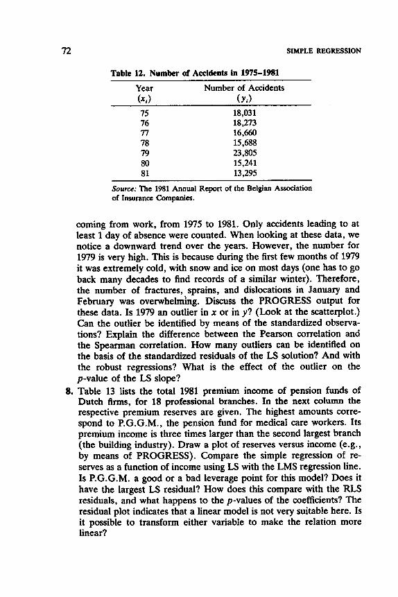
72
Table 12. Number of Accidents in 1975-1981
SIMPLE REGRESSION
Year Number of Accidents (4 ( Y i )
75 18,031 76 18,273 77 16,660 78 15,688 79 23,805 80 15,241 81 13,295
Source: "he 1981 Annual Report of the Belgian Association of Insurance Companies.
coming from work, from 1975 to 1981. Only accidents leading to at least 1 day of absence were counted. When looking at these data, we notice a downward trend over the years. However, the number for 1979 is very high. This is because during the first few months of 1979 it was extremely cold, with snow and ice on most days (one has to go back many decades to find records of a similar winter). Therefore, the number of fractures, sprains, and dislocations in January and February was overwhelmhg. Discuss the PROGRESS output for these data. Is 1979 an outlier in x or in y? (Look at the scatterplot.) Can the outlier be identified by means of the standardized observa- tions? Explain the difference between the Pearson correlation and the Spearman correlation. How many outliers can be identified on the basis of the standardized residuals of the LS solution? And with the robust regressions? What is the effect of the outlier on the p-value of the LS slope?
8. Table 13 lists the total 1981 premium income of pension funds of Dutch Arms, for 18 professional branches. In the next column the respective premium reserves are given. The highest amounts corre- spond to P.G.G.M., the pension fund for medical care workers. Its premium income is three times larger than the second largest branch (the building industry). Draw a plot of reserves versus income (e.g., by means of PROGRESS). Compare the simple regression of re- serves as a function of income using LS with the LMS regression line. Is P.G.G.M. a good or a bad leverage point for this model? Does it have the largest LS residual? How does this compare with the RLS residuals, and what happens to the p-values of the coefficients? The residual plot indicates that a linear model is not very suitable here. Is it possible to transform either variable to make the relation more linear?

EXERCISES AND PROBLEMS 73
Table 13. Pension Funds for 18 Professional Branches
Index Premium Income" Premium Reserves" ~~
1 2 3 4 5 6 7 8 9
10 11 12 13 14 15 16 17 18
10.4 15.6 16.2 17.9 37.8 46.9 52.4 52.9 71.0 73.9 76.3
' 77.0 131.2 151.7 206.1 314.7 470.8
1406.3
272.2 212.9 120.7 163.6 226.1 622.9
1353.2 363.6 951.7 307.2 588.4 952.5
1157.3 2105.6 3581.4 3404.7 4095.3 6802.7
"In millions of guilders. Source: de Wit (1982, p. 52).
Sections 5 and 6
9. Run the exact fit example of Section 5 again as a simple regression through the origin.
10. Look for an example where a line through the origin is more appropriate (from subject-matter knowledge) than with intercept.
11. Repeat exercise 8 (on the pension funds of 18 professions) by means of simple regression without intercept. This makes sense because the RLS intercept was not significantly different from zero. Draw the corresponding lines through the origin. Which transformation do you propose to linearize the data?
Section 7
12. Apply the resistant line (7.1), Theil's estimator (7.2), and the repeated median (7.4) to the monthly payments data (Table 1 of Chapter 1).
13. In the framework of simple regression, Hampel (1975, p. 379) considered the line through (medi x i , medi y i ) which has equal num-

74 SIMPLE REGRESSION
bers of positive residuals on both sides of medj xi . (He then dismissed this estimator by stating that it may lead to a lousy fit.) Simon (1986) proposed the “median star” line, which also goes through (med, x,, medi y j ) and has the slope
i?, = med I ( yi xi - -medxj m7d y7 * I
Show that this is the same estimator. What is its breakdown point? Write a small program and apply it to the situations of Figures 11 and 12. Repeat this for another version of the median star in which the intercept is chosen so that rned, (ri) = 0.
14. (Research problem). Is it possible to construct a standardized version of the breakdown plot, which does not depend on random number generation?

C H A P T E R 3
Multiple Regression
1. INTRODUCTION
In multiple regression, the response variable y i is related to p explanatory variables xil, . . . , xip in the model
yi = xilel + - - - + xipep + ei (i = 1, . . . , 4 .
As in simple regression, the least squares (LS) technique for estimat- ing the unknown parameters e,, . . . , Op is quite sensitive to the presence of outlying points. The identification of such points becomes more difficult, because it is no longer possible to spot the influential points in a scatterplot. Therefore, it is important to have a tool for identifying such points.
In the last few decades, several statisticians have given consideration to robust regression, whereas others have directed their attention to regres- sion diagnostics (see Chapter 6). Both approaches are closely related by two important common aims, namely, identifying outliers and pointing out inadequacies of the model. However, they proceed in a different way. Regression diagnostics first attempt to identify points that have to be deleted from the data set, before applying a regression method. Robust regression tackles these problems in the inverse order, by designing estimators that dampen the impact of points that would be highly influential otherwise. A robust procedure tries to accommodate the majority of the data. Bad points, lying far away from the pattern formed by the good ones, will consequently possess large residuals from the robust fit. So in addition to insensitivity to outliers, a robust regression estimator makes the detection of these points an easy job. Of course, the residuals from LS cannot be used for this purpose, because the outliers
75
Robust Regression and Outlier Detection Peter J. Rousseeuw, Annick M. Leroy
Copyright 0 1987 John Wiley & Sons, Inc. ISBN: 0-471-85233-3

76 MULTIPLE REGRESSION
may possess very small LS residuals as the LS fit is pulled too much in the direction of these deviating points.
Let us look at some examples to illustrate the need for a robust alternative to LS. The first example is the well-known stackloss data set presented by Brownlee (1965). We have selected this example because it is a set of real data and it has been examined by a great number of statisticians (Draper and Smith 1966, Daniel and Wood 1971, Andrews 1974, Andrews and Pregibon 1978, Cook 1979, Dempster and Gasko- Green 1981, Atkinson 1982, Carroll and Ruppert 1985, Li 1985, and many others) by means of several methods. The data describe the operation of a plant for the oxidation of ammonia to nitric acid and consist of 21 four-dimensional observations (listed in Table 1). The stackloss (y) has to be explained by the rate of operation ( x , ) , the cooling water inlet temperature (x2 ) , and the acid concentration ( x 3 ) . Summarizing the findings cited in the literature, it can be said that most
Table 1. Stackloss Data
Index Rate Temperature Acid Concentration Stackloss
1 80 27 89 42 2 80 27 88 37 3 75 25 90 37 4 62 24 87 28 5 62 22 87 18 6 62 23 87 18 7 62 24 93 19 8 62 24 93 20 9 58 23 87 15
10 58 18 80 14 11 58 18 89 14 12 58 17 88 13 13 58 18 82 11 14 58 19 93 12 15 50 18 89 8 16 50 18 86 7 17 50 19 72 8 18 50 19 79 8 19 50 20 80 9 20 56 20 82 15 21 70 20 91 15
(i) (Xt 1 ( x 2 ) (x3 1 (Y)
Source: Brownlee (1965).

INTRODUCTION 77
people concluded that observations 1,3,4, and 21 were outliers. Accord- ing to some people, observation 2 is reported as an outlier too. Least squares regression yields the equation
y^ = 0 . 7 1 6 ~ ~ + 1 . 2 9 5 ~ ~ - 0 . 1 5 2 ~ ~ - 39.9.
The LS index plot is shown in Figure 1. The standardization of the residuals is performed by the division of the raw residuals (ti = yi - 9,) by the scale estimate corresponding to the fit. A horizontal band encloses the standardized residuals between -2.5 and 2.5. In Figure 1, no outliers strike the eye. From the LS index plot, one would conclude that the data set contains no outliers at all because all the standardized LS residuals fall nicely within the band. However, let us now look at Figure 2, the index plot associated with the least median of squares (LMS) fit
F = 0 . 7 1 4 ~ ~ + 0.357~~ + 0.000x3 - 34.5 .
This plot is based on a robust fit, and does indeed reveal the presence of harmful points. From this index plot it becomes immediately clear that

78 MULTIPLE REGRESSION
Figure 2. Stackloss data: Index plot associated with LMS.
the observations 1, 3, 4, and 21 are the most outlying, and that case 2 is intermediate because it is on the verge of the area containing the outliers. This shows how our robust regression technique is able to analyze these data in a single blow, which should be contrasted to some of the earlier analyses of the same data set, which were long and laborious.
This example once more illustrates the danger of merely looking at the LS residuals. We would like to repeat that it is necessary to compare the standardized residuals of both the LS and the robust method in each regression analysis. If the results of the two procedures are in substantial agreement, then the LS can be trusted. If they differ, the robust technique can be used as a reliable tool for identifying the outliers, which may then be thoroughly investigated and perhaps corrected (if one has access to the original measurements) or deleted. Another possibility is to change the model (e.g., by adding squared or cross-product terms and/or transforming the response variable). In this way, Atkinson (1985, pp. 129-136) analyzes the stackloss data by setting up models explaining log(y) by means of xI, x 2 , x1x2, and x:.
The following example comes from the social sciences. The data set contains information on 20 schools from the Mid-Atlantic and New England states, drawn from a population studied by Coleman et al.

INTRODUCTION 79
(1966). Mosteller and Tukey (1977) analyze this sample consisting of measurements on six different variables, one of which will be treated as response. They can be described as follows:
x1 = staff salaries per pupil x2 = percent of white-collar fathers x 3 = socioeconomic status composite deviation: means for family size,
family intactness, father’s education, mother’s education, and home items
x4 = mean teacher’s verbal test score x5 = mean mother’s educational level (one unit is equal to two school
y = verbal mean test score (all sixth graders). years) ’
The data set itself is exhibited in Table 2.
Table 2. Coleman Data Set, Containing Information on 20 Schools from the Mid-Atlantic and New England States
Index
1 2 3 4 5 6 7 8 9
10 11 12 13 14 15 16 17 18 19 20
X1 x2
3.83 28.87 2.89 20.10 2.86 69.05 2.92 65.40 3.06 29.59 2-07 44.82 2.52 77.37 2.45 24.67 3.13 65.01 2.44 9.99 2.09 12.20 2.52 22.55 2.22 14.30 2.67 31.79 2.71 11.60 3.14 68.47 3.54 42.64 2.52 16.70 2.68 86.27 2.37 76.73
~
X , XA X . Y
7.20 -11.71
12.32 14.28 6.31 6.16
12.70 -0.17
9.85 -0.05
-12.86 0.92 4.77
-0.96 -16.04
10.62 2.66
- 10.99 15.03 12.77
26.60 6.19 24.40 5.17 25.70 7.04 25.70 7.10 25.40 6.15 21.60 6.41 24.90 6.86 25.01 5.78 26.60 6.51 28.01 5.57 23.51 5.62 23.60 5.34 24.51 5.80 25.80 6.19 25.20 5.62 25.01 6.94 25.01 6.33 24.80 6.01 25.51 7.51 24.51 6.96
37.01 26.51 36.51 40.70 37.10 33.90 41.80 33.40 41.01 37.20 23.30 35.20 34.90 33.10 22.70 39.70 31.80 31.70 43.10 41.01
Source: Mosteller and Tukey (,1977).

80 MULTIPLE REGRESSION
The ordinary LS regression for all 20 schools is given as
F = -1.79x, +0.044x,+0.556x,+1.11x4-1.81x5+19.9.
Least median of squares regression yields the fit
The left side of Table 3 lists the LS estimates and the associated residuals. These results reveal that the LS equation slightly overestimates the re- sponse for schools 3 and 11 and underestimates it for school 18. By only examining the LS results, the conclusion would be that schools 3, 11, and 18 are furthest away from the linear model. But from the right side of Table 3, it appears that school 11 does not deviate at all from the robust fit.
The robust regression spots schools 3, 17, and 18 as outliers by assigning large standardized residuals to them. Afterwards these standar-
Table 3. Coleman DaW. Estimated Verbal Mean Test Score and the Associated Residuals for the LS Fit and the LMS Fit
LS Results LMS Results
Estimated Standardized Estimated Standardized Index Response Residuals Response Residuals Weights
1 36.661 0.17 38.883 -1.59 1 2 26.860 -0.17 26.527 -0.01 1 3 40.460 -1.90 41.273 -4.04 0 4 41.174 -0.23 42.205 -1.28 1 5 36.319 0.38 37.117 -0.01 1 6 33.986 -0.04 33.917 -0.01 1 7 41.081 0.35 41.628 0.15 1 8 33.834 -0.21 32.922 0.41 1 9 40.386 0.30 41.519 -0.43 1
10 36.990 0.10 34.847 2.00 1 11 25.508 -1.06 23.169 0.11 1 12 33.454 0.84 33.514 1.43 1 13 35.949 -0.51 34.917 -0.01 1 14 33.446 -0.17 32.591 0.43 1 15 24.479 -0.86 22.717 -0.01 1 16 38.403 0.63 40.041 -0.29 1 17 33.240 -0.69 35.121 - -2.82 0 18 26.698 2.41 24.918 _. 5.76 0 19 41.977 0.54 42.662 0.37 1 20 40.747 0.13 41.027 -0.01 1

INTRODUCTION 81
dued residuals are used for computing weights, by giving a weight of 0 to all observations that have an absolute standardized residual larger than 2.5. Doing this for Coleman’s data set gives rise to the last column in Table 3. These weights are then employed for a reweighted least squares (RLS) analysis. This amounts to the same thing as performing LS regression on the reduced data set containing only the 17 points with a weight of 1.
Apart from the fitted equation and the associated residuals, outliers also affect the t-based significance levels. This is important for the construction of confidence intervals and for hypothesis testing about regression coefficients (see also Section 3 of Chapter 2). For the Coleman data set, the significance of the regression coefficients turns out to be quite different in the LS fit and the RLS fit. The t-values in Table 4 test the null hypothesis H,: 9 = 0 against the alternative H,: 9 # 0 for the LS estimates. From this table it is seen that only the variables x g and x , have LS regression coefficients that are significantly different from zero for a = 5%, because their t-values exceed the critical value 2.1448 of the Student distribution with 14 (= n - p) degrees of freedom, and hence their p-values are below 0.05.
Let us now analyze these data with the RLS using the weights of Table 3. This gives rise to the coefficients and t-values on the right side of Table 4. It is striking that for the cleaned data set, all the explanatory variables now have regression coefficients significantly different from zero for a = 5% (because the 97.5% quantile of a t-distribution with 11 degrees of freedom equals 2.2010, so all p-values are less than 0.05).
As in Chapter 2, it must be noted that the opposite can also happen. In many examples, the “significance” of certain LS regression coefficients is only caused by an outlier, and then the corresponding RLS coefficients may no longer be significantly different from zero.
The ordinary LS method is not immune to the masking effect. This means that after the deletion of one or more influential points, another
Table 4. Coleman Data: t-Values Assodated with the LS and the RLS Fit
LS Results RLS Reults
Variable Coefficient t-Value p-Value Coefficient t-Value p-Value
X1 -1.793 -1.454 0.1680 -1.203 -2.539 0.0275 x2 0.044 0.819 0.4267 0.082 4.471 O.ooo9 x3 0.556 5.979 0 . m 0.659 19.422 O.oo00 x4 1.110 2.559 0.0227 1.098 7.289 O.oo00
Constant 19.949 1.464 0.1652 29.750 6.095 0.0001 xs -1.810 -0.893 0.3868 -3.898 -5.177 0.0003

82 MULTIPLE REGRESSION
observation may emerge as extremely influential, which was not visible at first, Therefore, the use of a high-breakdown regression method (such as the LMS) for the determination of the weights is indispensable. As an illustration, let us consider the “Salinity data” (Table 5 ) that were listed by Ruppert and Carroll (19qO). It is a set of measurements of water salinity (i.e., its salt concentration) and river discharge taken in North Carolina’s Pamlico Sound. We will fit a linear model where the salinity is regressed against salinity lagged by two weeks (q), the trend, that is, the number of biweekly periods elapsed since the beginning of the spring
Table 5. Salinity Data
Index Lagged Salinity Trend Discharge Salinity (4 (XI 1 (x1) (x3) ( Y )
1 2 3 4 5 6 7 8 9
10 11 12 13 14 15 16 17 18 19 20 21 22 23 24 25 26 27 28
8.2 7.6 4.6 4.3 5.9 5.0 6.5 8.3
10.1 13.2 12.6 10.4 10.8 13.1 13.3 10.4 10.5 7.7
10.0 12.0 12.1 13.6 15.0 13.5 11.5 12.0 13.0 14.1
4 5 0 1 2 3 4 5 0 1 2 3 4 5 0 1 2 3 0 1 4 5 0 1 2 3 4 5
23.005 23.873 26.417 24.868 29.895 24.200 23.215 21.862 22.274 23.830 25.144 22.430 21.785 22.380 23.927 33.443 24.859 22.686 21.789 22.041 21.033 21.005 25.865 26.290 22.932 21.313 20.769 21.393
7.6 7.7 4.3 5.9 5.0 6.5 8.3 8.2
13.2 12.6 10.4 10.8 13.1 12.3 10.4 10.5 7.7 9.5
12.0 12.6 13.6 14.1 13.5 11.5 12.0 13.0 14.1 15.1
Source: Ruppert and Carroll (1980).

INTRODUCTION 83
season (xz); and the volume of river discharge into the sound (x3) . Carroll and Ruppert (1985) describe the physical background of the data. They indicated that cases 5 and 16 correspond to periods of very heavy discharge. Their analysis showed that the third and sixteenth observations conspire to hide the discrepant number 5. In fact, observation 5 can be recognized as influential only after the deletion of cases 3 and 16. This is a prime example of the masking effect. On the other hand, the LMS is not affected by this phenomenon and identifies 5 and 16 in a single blow. The LS fit is given by
y^ = 0 .777~~ - 0 . 0 2 6 ~ ~ - 0 . 2 9 5 ~ ~ + 9.59 ,
whereas the LMS yields the equation
A residual plot associated with the LS fit is presented in Figure 3. In this figure the standardized residuals are plotted against the estimated response. In Figure 4 such a residual plot is given for the LMS regression. From Figure 3, it appears that there is nothing wrong with the fit. However, one has to keep in mind that leverage points tend to produce small LS residuals simply by virtue of their leverage. On the other hand,
I- 0
Estimated response
Figure 3. Salinity data: Residual plot associated with the LS fit.

84 MULTIPLE REGRESSION
Estimated response
Figure 4. Salinity data: Residual plot associated with the LMS fit.
Figure 4 gives evidence of the presence of outlying observations, because some points fall far from the band. In this example, the LS residual plot cannot be trusted because it differs too much from the one associated with a robust fit.
As we said before, residual plots can also indicate possible defects in the model’s functional form in the direction of the fitted values. A residual plot may, for example, display a variance pattern that is a monotone function of the response. If the functional part of the model is not misspecified, then plotting the standardized LMS residuals versus ji gives rise to a horizontal band of points that look “structureless.” Also, anomalies in the pattern might suggest a transformation of the variables in the model. For example, a curved pattern in a residual plot may lead to replacing the observed yi by some function of y i (log yi or yi raised to some power). In example 2 of Section 3 we will illustrate the use of residual plots to remedy model failures.
2. COMPUTATION OF LEAST MEDIAN OF SQUARES MULTIPLE REGRESSION
The question “How do we run program PROGRESS?” has for the most part been answered in Section 2 of Chapter 2, in the context of simple

COMPUTATION OF LEAST MEDIAN OF SQUARES MULTIPLE REGRESSION 85
regression. The interactive session accompanying a multiple regression analysis is completely identical.
The special treatment of data sets with missing values has not yet been discussed. In that case the interactive input becomes a little bit longer. We will illustrate this situation for part of the “Air Quality” data that originated with the New York State Department of Conservation and the National Weather Service; these data were reported in Chambers et al. (1983). The whole data set consists of daily readings of air quality values from May 1, 1973 to September 30, 1973. We will use only the values for May in our example. The variables are the mean ozone concentration (in parts per billion) from 1300 to 1500 hours at Roosevelt Island (OZONE ppb), solar radiation in Longleys in the frequency band 4000-7700A from 0800 to 1200 hours at Central Park (SOLAR RADI), average wind speed (in miles per hour) between 0700 and lo00 hours at La Guardia Airport (WINDSPEED), and maximum daily temperature (in degrees Fahrenheit) at La Guardia Airport (TEMPERATUR). The data are exhibited in Table 6.
The aim of the analysis is to explain the ozone concentration by means of the other variables. In Table 6, one can observe that the measurements for OZONE ppb and/or SOLAR RADI are not registered for some days. PROGRESS provides two methods for handling such an incomplete data set. One or the other can be chosen by answering 1 or 2 to the question
CHOOSE AN OPTION FOR THE TREATMENT OF MISSING VALUES
O=THERE ARE NO MISSING VALUES IN THE DATA l=ELIMINATION OF THE CASES FOR WHICH AT LEAST ONE VARIABLE IS MISSING P=ESTIMATES ARE FILLED IN FOR UNOBSERVED VALUES ENTER YOUR CHOICE:
.......................................
When the option for missing values is not equal to zero, PROGRESS needs additional information on the missing value codes for each vari- able. First of all, the question
IS THERE A UNIQUE VALUE WHICH IS TO BE INTERPRETED AS A MISSING MEASUREMENT FOR ANY VARIABLE? ANSWER YES OR NO:
must be answered. When the answer is YES, the statement
PLEASE ENTER THIS VALUE:
appears, where the user has to give a value that will be interpreted as the

Table 6. Air Quality Data Set for May 1973"
Index SOLAR RADI WINDSPEED TEMPERATUR OZONE ppb ti) (4 (4 (4 t Y) 1 2 3 4 5 6 7 8 9
10 11 12 13 14 15 16 17 18 19 20 21 22 23 24 25 26 27 28 29 30 31
190 118 149 313
9999 9999 299 99 19
194 9999 256 290 274 65
334 307 78
322 44 8
320 25 92 66
266 9999
13 252 223 279
7.4 8.0
12.6 11.5 14.3 14.9 8.6
13.8 20.1 8.6 6.9 9.7 9.2
10.9 13.2 11.5 12.0 18.4 11.5 9.7 9.7
16.6 9.7
12.0 16.6 14.9 8.0
12.0 14.9 5.7 7.4
67 72 74 62 56 66 65 59 61 69 74 69 66 68 58 64 66 57 68 62 59 73 61 61 57 58 57 67 81 79 76
41 36 12 18
999 28 23 19 8
999 7
16 11 14 18 14 34 6
30 11 1
11 4
32 999 999 999 23 45
115 37
"The values 9999 of x , (solar radiation) indicate missing measurements. Also the numbers 999 of y (ozone ppb) correspond to missing values. Source: Chambers et al. (1983).
86

COMPUTATlON OF LEAST MEDIAN OF SQUARES MULTIPLE REGRESSION 87
missing value code for all the variables in the analysis. Otherwise, the user has to answer the following question for each variable:
I
W E S VARIABLE. . . . . . . . . . CONTAIN MISSING VALUE(S)? ANSUER YES OR NO:
(Instead of the dots, the actual label of the variable concerned will be printed.) If the answer to this question is YES, then the user has to enter the missing value code for this variable:
ENTER TEE VALUE OF THIS VARIABLE WRICH HAS TO BE INTERPRETED AS THE MISSING VALUE CODE:
In both missing value options, the program makes an inventory of the cases with incomplete data, for each variable for which missing values were announced. When there are variables for which more than 80% of the cases have a missing value, the program will terminate (after giving a message). When analyzing the same data again, the user should no longer include these partially observed variables because they do not contain enough information.
Let us now look at the two missing value options provided by PROGRESS. The first avenue open to the researcher is to eliminate the cases for which at least one variable is missing. This can be achieved by setting the missing value option equal to 1. When the print option differs from 0, a complete table is given, where for each case the user of the program can see which variables were missing. The regression analysis is then performed on the remaining cases. (Each case keeps its original number.)
In fact, this option can also be used for another purpose. It may happen that one wishes to perform the analysis only on a part of the data set. For example, in a sample containing attributes of many people, one may want to fit a linear model to the women only. Then one can use the missing value option 1 for the variable associated with the sex of each person. The value corresponding to men then has to be taken as the “missing” value code, in order to eliminate the observations for men.
An alternative treatment, which corresponds to option 2, consists of filling in guesses for unobserved values. This can be necessary in circum- stances where deleting all partially observed cases would result in an extremely small sample (which might even be empty). Nevertheless, even for this option, cases for which the response y is lacking will first be dropped from the data set. Also, cases for which all explanatory variables are missing will be removed. On this reduced data set, missing data will

88 MULTIPLE REGRESSION
be replaced by the median of the corresponding variable. On the resulting data set, the previous methods of estimation can be applied. When the print option is not 0, the output of PROGRESS delivers a complete inventory of the deleted cases and of the missing values that are replaced by medians. Also here, the cases retain the numbering of the original data set.
For the Air Quality data, we encoded the missing values of variable SOLAR RADI by 9999, and those of OZONE ppb by 999. These codes are acceptable because these values have not been observed. Let us now look at a listing of the interactive input for this data set.
D O I W YES OR
VAlT TO m: 10
OUTL I ER DIAGSCSTICB 7
OIVE "HB .AXE OF THE FILE CQlfAIWIIQ THE DATA (0.6. TYPB A:BXAHPLE.DAT ) , ot TYPE ICEY IF YOU PREFER TO EITER THE DATA BY KBYBOARD. VHAT m YOU CHOOSE 7 B: AIRMY. DAT

COMPUTATION OF LEAST MEDIAN OF SQUARES MULTIPLE REGRESSION 89
WIERB DO YOU VAIT YOUR OUTPUT? .............................. TYPE COI IF YOU VAIT IT 01 THE GCBBB.
or TYPB PEU IF YOU VAIT IT O I TRB PRIBTEE or TYPB TfIE IAHB OF A FILB (0.5. B:BXASF%B.OUT) (VMWIIQ : IF THBBB ALREADY EXISTS A FILB VITE THE SANE I A 1 I I I
TEE OLD FILB VILL BE OVERVRITfEI.> VBI? YOU ~80088 B:AIRHAY.RES
VHICH VERSIOI OF THE ALOORlTHJI VOULD YOU LIKE TO USE?
Q = QUICK VERSIOI E - EXTEISIW SEARCH BBTER YOUR CHOICE PLEASE <Q OR E> : E
CEOOSH AS OPT101 W R THE TREATHEIT OF HISSIIC VALUES
0 - THERE ARE HISSIIC VALUES I 1 THE DATA 1 - ELIHIIATIOU OF THE CASES FOR YHICH AT LEAST OBB VARIABLE IS HISSIIC 2 - BSIIIIATES ARE PILLBD 11 FOR UXOBSERVED VALUES H.TBR YOUR CHOICE : 1
.....................................................
....................................................
. . . . . . . . . . . . . . . . . . . . . . . . . . . . . . . . . . . . . . . . . . . . . . . . . . . . . . . . . . . . . . . . * P R 0 0 R E 8 S VILL PRRWRH A RECRESSIOI VITH COBSTAFT TERH * . . . . . . . . . . . . . . . . . . . . . . . . . . . . . . . . . . . . . . . . . . . . . . . . . . . . . . . . . . . . . . . . . THE IIIIIIBER OF CASES EQUALS 31
Ozow ppb YOUR DATA RESIDE OI FILE : B: AIRHAY. DAT TITLE FOR OUTPUT : AIR QUALITY WASURENBSTS FOR .EV YORK THE DATA VILL BE READ I 1 FREE FORHAT. LARGE OUTPUT IS VAlTED. BOTH TYPES OF RESIDUAL PLOTS ARE VMTED. THE EXTEmIVE SEARCH ALOORITHH VILL BE USED. TREATHEIT OF HISSIUC VALUES 1% OPTIOU 1: THIS WAIS THAT A CASH VITH A HISSIIC VALUE FOR AT LEAST OSE VARIABLE VILL BE DELETED. YOUR OUTPUT VILL BE VRITTEI 011 : B:AIR?UY.RBS
ARE ALL THESE OPTIO.6 OK ? YES OR YO : YES
18 THERE A WEIQUE VALUE YHlCB IS TO BE IITERPRETED AS A HISSIIC NEASUREHEBT FOR A Y Y VARIABLE? AmSVER YES OR 10 : UO DOES VARIABLE SOLAR RADX COITAIU HISS110 VALUECS)?
EBTER THE VALUE OF THIS VARIABLE VHICH HAS TO BE IXTERPRETED AS TEE XI88110 VALUE CODE : 9999 DOES VARIABLE VISDSPEED COBTAII NISSIIC VALUE<S>? AIGVBR YES OR YO : I0 DOES VARIABLE TENPERATUR COBTAII HISSIIG VALUE(S>? AISVBR YPS OR .O : BO DOES THE RESPOISB VARIABLB COETAII HISSIBC VALUB(S>? AISVER YES OR 10 : YES BITER THE VALUE OF THIS VARIABLE YHICH HAS TO BE IBTERPRETED AS THE JIISSIIC VALUE CODE : 999
THE MlBER OF EXPLAIATORY VARIABLES EQUALS 3 IS THE RESF'OPSE VARIABLE.
A I ~ R YES OR so : YES

90 MULTIPLE REGRESSION
The treatment of the missing values for this data set appears on the output of PROGRESS as follows:
TREATNEWT OF HISSIBG VALUES IB OPTIOB 1: THIS NEABS THAT A CASE VITH A NISSIBG VALUE FOR AT LEAST ORE VARIABLE VILL BE DELETED.
YOUR DATA RESIDE OB FILE : B: AIRNAY. DAT VARIABLE SOLAR RADI H A S A HISSIBG VALUE FOR 4 CASES. VARIABLE OZOBE ppb H A S A NISSIBG VALUE FOR 5 CASES.
CASE HAS A HISSIBG VALUE FOR VARIABLES (VARIABLE WHBER 5 IS THE RESFQBSE ---_ ----- ---- 5 1 5 6 1
10 5 11 1 25 5 26 5 27 1 5
THERE ARE 24 CASES STAYIBG IB THE ABALYSIS. THE OBSERVATIOBS. AFTER TREATXEBT OF WISSIHG VALUES :
SOLAR RADI VIBDSPEED TEMPERATUR OZOBE ppb 1 2 3 4 7 8 9
12 13 14 15 16 17 18 19 20 21 22 23 24 28 29 30 31
190.0000 118.0000 149.0000 313.0000 299.0000
99.0000 19.0000
256.0000 290.0000 274.0000 65.0000
334.0000 307.0000
78.0000 322.0000
44.0000 8.0000
320.0000 25.0000 92.0000 13.0000
252.0000 223.0000 279.0000
7.4000 8.0000
12.6000 11.5000 8.6000
13. 8000 20.1000
9.7000 9.2000
10.9000 13.2000 11.5000 12.0000 18.4000 11.5000 9.7000 9.7000
16.6000 9.7000
12.0000 12.0000 14.9000 5.7000 7.4000
67.0000 72.0000 74.0000 62.0000 65.0000 59.0000 61.0000 69.0000 66.0000 68.0000 58.0000 64.0000 66.0000 57.0000 68.0000 62.0000 59.0000 73.0000 61.0000 61.0000 67.0000 81.0000 79.0000 76.0000
41.0000 36.0000 12.0000 18.0000 23.0000 19.0000 8.0000
16.0000 11.0000 14.0000 18.0000 14.0000 34.0000
6.0000 30.0000 11.0000
1.0000 11.0000 4.0000
32.0000 23.0000 45.0000
115.0000 37.0000
The least squares analysis of the reduced data set is printed in Table 7. Some of the fitted OZONE ppb values (cases 9 and 18) are negative, which is physically impossible. The strange behavior of this fit is easy to understand when comparing it to the robust analysis in Table 8. First of all, the equations of both fits differ substantially from each other. In the

COMPUTATION OF LEAST MEDIAN OF SQUARES MULTIPLE REGRESSION 91
Table 7. Air Quality Dats: LS Fit with Estimated Response and Standardized Residuals ~ -~ ~~ ~
Variable Coefficient Standard Error t-Value
SOLAR RADI -0.01868 0.03628 -0.51502 WINDSPEED - 1.99577 1.14092 - 1.74926 TEMPERATUR 1.96332 0.66368 2.95823 Constant -79.99270 46.81654 - 1.70864
Index Estimated “OZONE ppb” Standardized Residuals
1 2 3 4 7 8 9
12 13 14 15 16 17 18 19 20 21 22 23 24 28 29 30 31
33.231 43.195 37.362 12.933 24.873 6.452
-0.700 31.334 25.807 26.639 6.321
16.468 19.901
-6.263 24.545 21.552 16.335 24.221 19.944 14.101 27.357 44.591 59.567 49.238
0.43 -0.40 -1.41
0.28 -0.10
0.70 0.48
-0.85 -0.82 -0.70
0.65 -0.14
0.78 0.68 0.30
-0.59 -0.85 -0.73 -0.89
0.99 -0.24
0.02 3.08
-0.68
column comprising the standardized residuals in Table 8, case 30 emerges as an outlier. This single outlier is the cause of the bad LS fit because it has tilted the LS hyperplane in its direction. Because of this, the other points are not well fitted anymore by LS.
Of course, negative predicted values are to be expected whenever a linear equation is fitted. Indeed, when the regression surface is not horizontal, there always exist vectors x for which the corresponding

92 MULTIPLE REGRESSION
Table 8. Air Quality Data: RLS Fit Based on LMS ~~~ ~~ ~~
Variable Coefficient Standard Error r-Value
SOLAR RADI 0.00559 0.02213 0.25255 WINDSPEED - 0.74884 0.71492 - 1.04745 TEMPERATUR 0.99352 0.4292% 2.31438 Constant -37.51613 28.95417 - 1.2957 1
Index Estimated “OZONE ppb” Standardized Residuals
1 24.571 1.52 2 28.686 0.68 3 27.402 -1.42 4 17.220 0.07 7 22.294 0.07 8 11.321 0.71 9 8.143 -0.01
12 25.204 -0.85 13 22.788 -1.09 14 23.413 -0.87 15 10.587 0.69 16 19.325 -0.49 17 20.786 1.22 18 5.772 0.02 19 23.232 0.63 20 17.065 -0.56 21 13.883 -1.19 22 24.369 - 1.24 23 15.965 -1.11 24 14.617 1.61 28 20.137 0.26 29 33.210 1.09 30 37.950 7.13 31 34.010 0.28
predicted 9 is negative. This is still true for robust regression, where one can easily encounter a negative qi in a leverage point xi. However, in the above example the LS predictions are negative in good observations!
3. EXAMPLES
In the preceding sections we have seen that the high-breakdown fits provide much to think about. In particular, the standardized residuals

EXAMPLES 93
associated with a robust fit yield powerful diagnostic tools. For example, they can be displayed in residual plots. These graphics make it easy to detect outlying values and call attention to model failures. Also, the residuals can be used to determine a weight for each point. Such weights make it possible to bound the effect of the outliers by using them for RLS. The fit resulting from this reweighting describes the trend followed by the majority of the data. The statistics associated with this fit, like r- and F-values, are more trustworthy than those calculated from the ordinary LS regression.
Example 1: Hawkins-Bmdu-Kass Data
We shall use the data generated by Hawkins, Bradu, and Kass (1984) for illustrating some of the merits of a robust technique. Such artificial data offer the advantage that at least the position of the bad points is known exactly, which avoids some of the controversies that are inherent in the analysis of real data. In this way, the effectiveness of the technique can be measured. The data set is listed in Table 9 and consists of 75 observations in four dimensions (one response and three explanatory variables). The first 10 observations are bad leverage points, and the next four points are good leverage points (i.e., their xi are outlying, but the corresponding yi fit the model quite well). We will compare the LS with our robust regression. In Hawkins et al. (1984), it is mentioned that M-estimators do not produce the expected results, because the outliers (the bad leverage points) are masked and the four good leverage points appear outlying because they possess large residuals from those fits. This should not surprise us, because M-estimators break down early in the presence of leverage points. A certain version of the “elemental sets” diagnostic of Hawkins et al. locates the outliers, but this technique would not have coped with a larger fraction of contamination. (More details about outlier diagnostics and their breakdown points will be provided in Chapter 6.)
Let us now restrict the discussion to LS and LMS. From the index plot associated with LS (see Figure 3, it appears that observations 11,12, and 13 are outliers because they fall outside the k2.5 band. Unfortunately, from the generation one knows that these are good observations. The bad leverage points have tilted the LS fit totally in their direction. Therefore the first 10 points have small standardized LS residuals. (The index plots associated with M-estimators are very similar to that of LS.) On the other hand, the index plot of the LMS (Figure 6) identifies the
first 10 points as the influential observations. The four good leverage points fall in the neighborhood of the dashed line through 0. This means that these points are well accommodated by the LMS fit. Clearly, the

Table 9. Artificial Data Set of Hawkins, Bradu, and Kass (1984)
Index x , x2 x , Y
1 2 3 4 5 6 7 8 9
10 11 12 13 14 15 16 17 18 19 20 21 22 23 24 25 26 27 28 29 30 31 32 33 34 35 36 37 38
10.1 19.6 28.3 9.5 20.5 28.9
10.7 20.2 31.0 9.9 21.5 31.7
10.3 21.1 31.1 10.8 20.4 29.2 10.5 20.9 29.1 9.9 19.6 28.8 9.7 20.7 31.0 9.3 19.7 30.3
11.0 24.0 35.0 12.0 23.0 37.0 12.0 26.0 34.0 11.0 34.0 34.0 3.4 2.9 2.1 3.1 2.2 0.3 0.0 1.6 0.2 2.3 1.6 2.0 0.8 2.9 1.6 3.1 3.4 2.2 2.6 2.2 1.9 0.4 3.2 1.9 2.0 2.3 0.8 1.3 2.3 0.5 1.0 0.0 0.4 0.9 3.3 2.5 3.3 2.5 2.9 1.8 0.8 2.0 1.2 0.9 0.8 1.2 0.7 3.4 3.1 1.4 1.0 0.5 2.4 0.3 1.5 3.1 1.5 0.4 0.0 0.7 3.1 2.4 3.0 1.1 2.2 2.7 0.1 3.0 2.6 1.5 1.2 0.2
9.7 10.1 10.3 9.5
10.0 10.0 10.8 10.3 9.6 9.9
-0.2 -0.4
0.7 0.1
-0.4 0.6
-0.2 0.0 0.1 0.4 0.9 0.3
-0.8 0.7
-0.3 -0.8 -0.7
0.3 0.3
-0.3 0.0
-0.4 -0.6 -0.7
0.3 -1.0 -0.6
0.9
Index x , x , x , Y
39 40 41 42 43 44 45 46 47 48 49 so 51 52 53 54 55 56 57 58 59 60 61 62 63 64 65 66 67 68 69 70 71 72 73 74 75
2.1 0.0 1.2 0.5 2.0 1.2 3.4 1.6 2.9 0.3 1.0 2.7 0.1 3.3 0.9 1.8 0.5 3.2 1.9 0.1 0.6 1.8 0.5 3.0 3.0 0.1 0.8 3.1 1.6 3.0 3.1 2.5 1.9 2.1 2.8 2.9 2.3 1.5 0.4 3.3 0.6 1.2 0.3 0.4 3.3 1.1 3.0 0.3 0.5 2.4 0.9 1.8 3.2 0.9 1.8 0.7 0.7 2.4 3.4 1.5 1.6 2.1 3.0 0.3 1.5 3.3 0.4 3.4 3.0 0.9 0.1 0.3 1.1 2.7 0.2 2.8 3.0 2.9 2.0 0.7 2.7 0.2 1.8 0.8 1.6 2.0 1.2 0.1 0.0 1.1 2.0 0.6 0.3 1.0 2.2 2.9 2.2 2.5 2.3 0.6 2.0 1.5 0.3 1.7 2.2 0.0 2.2 1.6 0.3 0.4 2.6
-0.7 -0.5 -0.1 -0.7
0.6 -0.7 -0.5 -0.4 -0.9
0.1 0.9
-0.4 0.7
-0.5 0.7 0.7 0.0 0.1 0.7
-0.1 -0.3 -0.9 -0.3
0.6 -0.3 -0.5
0.6 -0.9 -0.7
0.6 0.2 0.7 0.2
-0.2 0.4
-0.9 0.2
94

- I l l l ~ l l l l ~ I l " ~ l l I j
- - 2.5 ' -
(D a z K
-2.5
95
- -
14 0
13
- - '
- 11. - - 12.
- - - - 3
I l l 1 , 1 1 1 I 1 I I I I I l l
LI 1 I I I I I I I I I I 1 I I I I - ,
-
-
- 0)
(D 0
- - - 1" 2 E 8 K 2.5 r m
- - -

96 MULTIPLE REGRESSION
conclusions drawn from the LMS index plot agree with the construction of the data.
The following example illustrates the use of residual plots for model specification.
Example 2: Cloud Point Data
Table 10 shows a set of measurements concerning the cloud point of a liquid (Draper and Smith 1966, p. 162). The cloud point is a measure of the degree of crystallization in a stock and can be measured by the refractive index. The purpose is to construct a model where the percen- tage of 1-8 in the base stock can be used as a predictor for the cloud point. Because the data contain only two variables, it is possible to explore the relation between these variables in a scatterplot. The scatter- plot associated with Table 10 can be found in Figure 7.
The curved pattern in Figure 7 indicates that a simple linear model is not adequate. We will now examine whether the residual plot associated
Table 10. Cloud Point of a Liquid
Index Percentage of 1-8 Cloud Point (9 (4 ( Y )
1 2 3 4 5 6 7 8 9
10 11 12 13 14 15 16 17 18 19
0 1 2 3 4 5 6 7 8 0 2 4 6 8
10 0 3 6 9
22.1 24.5 26.0 26.8 28.2 28.9 30.0 30.4 31.4 21.9 26.1 28.5 30.3 31.5 33.1 22.8 27.3 29.8 31.8
~~ ~~
Source: Draper and Smith (1969, p. 162).

EXAMPLES 97
8 8
8 8
0
0
e 0
20 I I I I I 1 1 1 1 1 1 1 1 1 1 1 1 1 1 1
0.0 2.5 5.0 7.5 10.0 Percentage of 1-8
Figure 7. Cloud point data: Scatterplot.
with the linear fit would have suggested this. From the residual plot of the LS line in Figure 8, it is clear that the straight-line fit is imperfect because the residuals appear not to be randomly distributed about the zero line.
In order to be sure that this pattern is not caused by the presence of outliers, we will compare Figure 8 to the residual plot associated with the RLS line (Figure 9). The departure from linearity is magnified in this plot. The residuals inside the k2.5 band tend to follow a parabolic curve. Those associated with cases 1, 10, and 16 fall outside the band, which indicates that they have large residuals from the RLS line. In spite of the fact that the slopes of both the LS and RLS lines are significantly different from zero (see the t-values in Table ll), the linear model is not appropriate.
Moreover, the value of R2, which is a measure of model adequacy, is high. For LS, R2 equals 0.955. The RLS value of R2 is 0.977, showing that 97.7% of the total variation in the response is accounted for by the explanatory variable. Of course, R2 is only a single number summary. It is not able to characterize an entire distribution or to indicate all possible defects in the functional form of the model. A large R2 does not ensure that the data have been well fitted. On the other hand, the residual plots do embody the functional part of the model. Therefore, inspection of

98

EXAMPLES 99
Table 11. Cloud Point Data: Estimated Slope and Intercept by LS and RLS Regression, with Their Nalues ~~~ ~ ~ ~
LS Results RLS Results
Standard Standard Variable 6 Error r-Value 6 Error r-Value
Percentage of 1-8 1.05 0.055 18.9 0.89 0.036 24.7 Constant 23.35 0.297 78.7 24.37 0.212 115.2
R2 = 0.955 R2 = 0.977
these plots is an indispensable part of regression analysis, even when R2 is large or in the case of significant t-values. When this graphical display reveals an unexpected pattern, one has to remedy the defect by adapting the model. Depending on the anomalies in the pattern of the residuals, it may happen that an additional explanatory variable is necessary, or that some variables in the model have to be transformed. The possible improved models have to be restricted to those that are linear in the coefficients, or else we leave the domain of linear regression. How- ever, several nonlinear functions are linearizable by using a suitable transformation. Daniel and Wood (1971) list various types of useful transformations.
A curved plot such as Figure 9 is one way to indicate nonlinearity. The usual approach to account for this apparent curvature is to consider the use of a quadratic model such as
y = e,x + q x 2 + e, + e . (3.1)
The LS and RLS estimates for this model are given in Table 12, along with some summary statistics.
The R2 values for both the LS and the RLS have increased a little bit, whereas the t-values of the regression coefficients have hardly changed. For both fits, the coefficients are significantly different from zero at a = 5%. Let us now look at the distribution of the residuals associated with LS and RLS, in Figures 10 and 11, respectively.
Examining the LS residual plot, it would appear that the additional squared term has not been completely successful in restoring the distribu- tion of the residuals. The pattern is not entirely neutral. Before deciding to change the model again, let us analyze the information provided by the RLS residual plot. From this plot, some outliers strike the eye. The observations 1, 10, and 15, which have obtained a zero weight from the LMS fit, fall outside the horizontal band. (Notwithstanding their zero

100 MULTIPLE REGRESSION
Table 12. Cloud Point Data: Ls and RLS Estimates for the Quadratic Model along with Summary Values
LS Results RLS Results
Standard Standard Variable 6 Error r-Value 6 Error &Value
Percentage of 1-8 1.67 0.099 16.9 1.57 0.084 18.8
Constant 22.56 0.198 113.7 22.99 0.172 133.7 (Percentage of I-8)2 -0.07 0.010 -6.6 -0.07 0.009 -7.5
R' = 0.988 R2 = 0.993
weights, the outliers are still indicated in the plot.) The presence of these points has affected the LS estimates because LS tries to make all the residuals small, even those associated with outliers, at the cost of an increased estimate of 0,. On the other hand, the outlying observations do not act upon the RLS estimates, at which they obtain a large residual. The residuals inside the band in Figure 11, which corre- spond to the other observations, display no systematic pattern of varia- tion. Summarizing the findings from Figures 10 and 11, one can conclude that the quadratic equation describes a more appropriate fit than the
Estimated response
Figure f0. Cloud point data: LS residual plot for the quadratic model.

EXAMPLES 101
1:;: , , , , , , , , , * 4 Estimated response
Figure 11. Cloud point data: RLS residual plot for the quadratic model.
simple line. Moreover, the residual plot of the RLS quadratic fit locates three observations that were responsible for the deformed pattern in the residual plot of the JS quadratic fit.
The presence of outliers or the choice of an appropriate model are not the only problems in regression analysis. A nearly linear dependence between two or more explanatory variables can also seriously disturb the estimated regression surface or make the regression coefficients uninter- pretable. This phenomenon is called multicollinearity. (The terms col- linearity and ill-conditioning are also employed in the literature.) The ideal situation would be that there is no relation among the variables in the factor space. In that case, it is easy to interpret a regression coefficient as the amount of change in the response when the correspond- ing explanatory variable grows with one unit, while the other explanatory variable(s) remain fixed. When collinearity is present in the data, the contribution of a single explanatory variable to the regression equation is hard to estimate.
The detection of multicollinearity may be very complicated. When there are only two explanatory variables, then collinearity leads to a high absolute value of the Pearson correlation or the alternative (more robust) Spearman rank correlation coefficient. For higher-dimensional factor spaces, the two-by-two correlation coefficients are not always sufficient

102 MULTIPLE REGRESSION
for discovering collinearity , because the collinearity may involve several variables. Therefore, the squared multiple correlation coefficients R; of the regression of xi on the remaining x-variables are possible diagnostics for measuring the degree to which any xi is related to the other explana- tory variables.
Chatterjee and Price (1977), Belsley et al. (1980), Weisberg (1980), and Hocking (1983), among others, report some tools for identifying collinearity. Most of these tools are based on the correlation matrix or its inverse. For example, the so-called Variance Inflation Factor (VIF) is based on the estimated variance of the ith regression coefficient (obtained from LS). There are some debates whether or not the data should be standardized first, because this may have a large effect on the resulting collinearity diagnostics (see the article by Belsley 1984 and its discussion). Another approach to deal with collinearity is ridge regression (Hoerl and Kennard 1970, 1981), based on the principle of using a little bit of all the variables rather than all of some variables and none of the remaining ones (Marquardt and Snee 1975). We will not describe these techniques in further detail here. Unfortunately, most of them are not immune to the presence of contamination, as was also noted by Mason and Gunst (1985) and Ercil(l986). For instance, consider the nonrobustness of the Pearson correlation coefficient, which may be affected a great deal by outliers. This means that the correlation coefficient can be close to zero because of the presence of a single outlier disturbing an otherwise linear relation- ship, thereby hiding collinearity. On the other hand, the correlation coefficient can also be camed arbitrarily close to 1 by means of a far outlier, which appears to create collinearity . Therefore, the identification of linear dependencies in factor space, combined with the detection of outliers, is an important problem of regression analysis. Indeed, col- linearity inflates the variance of the regression coefficients, may be responsible for a wrong sign of the coefficients, and may affect statistical inference in general. Therefore, in cases where the presence of collineari- ty is anticipated, we recommend the use of the classical collinearity diagnostics on both the original data set and on the reweighted one based on LMS, in which the outliers have been removed.
Example 3: Heart Catheterization Data
The “Heart Catheterization” data set of Table 13 (from Weisberg 1980, p. 218 and Chambers et al. 1983, p. 310) demonstrates some of the effects caused by collinearity .
A catheter is passed into a major vein or artery at the femoral region

EXAMPLES 103
Table 13. Heart Catheterization Data"
Index Height Weight Catheter Length (i) (XI) ( x * ) (Y)
1 2 3 4 5 6 7 8 9
10 11 12
42.8 63.5 37.5 39.5 45.5 38.5 43.0 22.5 37.0 23.5 33.0 58.0
40.0 93.5 35.5 30.0 52.0 17.0 38.5 8.5
33.0 9.5
21.0 79.0
37 50 34 36 43 28 37 20 34 30 38 47
~ ~~ - ~~
"Patient's height is in inches, patient's weight in pounds, and catheter length is in centimeters. Source: Weisberg (1980, p. 218).
and moved into the heart. The catheter can be maneuvered into specific regions to provide information concerning the heart function. This tech- nique is sometimes applied to children with congenital heart defects. The proper length of the introduced catheter has to be guessed by the physician. For 12 children, the proper catheter length ( y) was determined by checking with a fluoroscope that the catheter tip had reached the right position, The aim is to describe the relation between the catheter length and the patient's height (xl) and weight (x2). The LS computations, as well as those for RLS, for the model
are given in Table 14. For both regressions, the F-value is large enough to conclude that a1
and together contribute to the prediction of the response. Looking at the r-test for the individual regression coefficients, it follows that the LS estimate for 6, is not significantly different from zero at a = 5%. The same can be said for 4. However, the F-statistic says that the two x-variables viewed en bloc are important. For the RLS fit, 8, is not yet significantly different from zero, which means that the corresponding explanatory variable contributes little to the model. Also, the sign of Gl makes no sense in this context. Such phenomena typically occur in

104 MULTIPLE REGRESSION
Table 14. Heart Catheterization Data: J S and RLS Results
LS Results RLS Results
Variable 5 r-Value p-Value 5 r-Value p-Value
Height 0.211 0.6099 0.5570 -0.723 -2.0194 0.09oO Weight 0.191 1.2074 0.2581 0.514 3.7150 0.09 Constant 20.38 2.4298 0.0380 48.02 4.7929 0.0030
F = 21.267 ( D = O.OOO4) F = 32.086 ( p = O.OOO6)
situations where collinearity is present. Indeed, Table 15 shows the high correlations among the variables, as computed by PROGRESS.
The correlation between height and weight is so high that either variable almost completely determines the other. Morebver, the low r-value for the regression coefficients confirms that either of the explana- tory variables may be left out of the model. For the heart catheterization data, we will drop the variable weight and look at the simple regression of catheter length on height. A scatterplot of this two-dimensional data set is given in Figure 12, along with the LS and RLS fits.
The LS yields the fit 9 = 0.612~ + 11.48 (dashed line in Figure 12). The RLS fit 9 = 0.614~ + 11.11 (which now has a positive 8,) lies close to the Ls. Note that cases 5 , 6, 8, 10, and 11 lie relatively far from the RLS fit. Because they are nicely balanced above and below the RLS line, the LS and RLS fits do not differ visibly for this sample.
The alternative choice would be to use weight instead of height as our predictor. A plot of measurements of catheter length versus the patient’s weight is shown in Figure 13. This scatterplot suggests that a linear model
Table 15. Heart Catheterization Data: Correlations Between the Variables
Pearson Correlation Coefficients
Height 1.00 Weight 0.96 1.00 Catheter length 0.89 0.90 1.00
Height Weight Catheter length
Spearman Rank Correlation Coefficients
Height 1 .00 Weight 0.92 1 .00 Catheter length 0.80 0.86 1.00
Height Weight Catheter length

EXAMPLES 105
50
r: 40
al - ti c, al
0 30
30 40 50 60 Height
Figure 12. Heart catheterization data: Scatterplot of proper catheter length versus height for 12 children, with LS fit (dashed line) and RLS fit (solid line).
is not appropriate here. It is clear that a transformation is required. On physical grounds, one might try to use the cube root of the weight instead of the weight itself in order to obtain linearity.
Even when there is no evidence of multicollinearity, it may happen that the complete set of explanatory variables is too large for using them all in the model. In the first place, too many variables make it hard to understand the described mechanism. This should, however, be combined with the objective of explaining the variability of the response as much as possible, which leads to the consideration of more explanatory variables. But from a statistical point of view, one can sometimes say that the reduction of the number of variables improves the precision of the fit. Indeed, explanatory variables for which the associated regression coeffici- ents are not significantly different from zero may increase the variance of the estimates. Subject-matter knowledge is sometimes sufficient to decide which of the possible equations is most appropriate. Otherwise one has to apply a statistical procedure for finding a suitable subset of the variables. This problem is called vuriuble selection. It is closely linked to the problem of model specification, which we discussed above. Indeed, the problem of variable selection also includes the question, “In which form

106 MULTIPLE REGRESSION
501 0
0
0
0 0 rn
0
20
25 50 75 Weight
Figure 13. Heart catheterization data: Scatterplot of proper catheter length versus weight for 12 children.
should the explanatory variable enter the equation: as the original variable, or as a squared term, or as a logarithmic term, and so on?”. For simplicity, one usually treats these problems separately in order to avoid the ideal, but intractable, approach consisting of a simultaneous treat- ment of both problems. The presence of outliers, either in y or in x, complicates the situation even more. Therefore, we recommend starting the analysis with a high-breakdown regression on the full set of variables in order to determine the weights of the observations. Then, as a first approximation, one can use a classical technique for variable selection on the “cleaned” sample. Such variable selection techniques have been widely investigated in the literature, for instance by Aitkin (1W4), Allen (1974), Diehr and Hoflin (1974), Hill and Hunter (1974), Narula and Wellington (1977, 1979), Snee (1W7), Suich and Derringer (1977, 1980), Ellerton (1978), McKay (1979), Hintze (1980), Rencher and Pun (1980), Weisberg (1981), Wilkinson and Dallal (1981), Baskerville and Toogood (1982), Madsen (1982), and Young (1982). Hocking (1976) reviews the topic of variable selection. We will briefly describe the most widely used techniques.
When the set of candidate variables is not too large, one can consider

EXAMPLES 107
all the possible models starting from this set. This is the so-called all-subsets regression procedure. It leads to
2(number of available explanatory variables)
different models, a number that increases rapidly. Even when attention is focused on LS estimation (or our RLS, assuming that a very robust technique has been executed first), this number becomes computationally infeasible. This has motivated some people to develop more efficient algorithms, which appeal to numerical methods for calcdating the LS estimates for the successive subsets. Usually, these procedures are based on either Gauss-Jordan reduction or a sweep operator (Beaton 1964, Seber 1977). Once the various fitted equations are at one’s disposal, one needs a criterion for judging which subset of variables yields the “best” fit. Hocking (1976) describes different measures for this purpose, includ- ing the mean squared error, the coefficient of determination, and the C, statistic (see also Daniel and Wood 1971 and Mallows 1973 for a thorough treatment of C,). The Furnival and Wilson (1974) algorithm, which is available in the regression program P2R of BMDP, is a branch-and-bound type of procedure that cuts the computation time by searching only in certain promising directions.
Although it is felt that the investigation of all subsets produces the “best” set, it is not the most widely used method because of its computa- tional cost. The so-called stepwise procedures, which consist of either adding or deleting one explanatory variable at a time, have been the favorite methods throughout. One distinguishes forward selection and backward elimination stepwise procedures, and a combination of both. Variations of these types have been implemented in several statistical packages, such as BMDP, SAS, and SPSS.
In forward selection, one starts with a simple regression model in which the explanatory variable is the variable that correlates best with the response. Then, at each subsequent step, one adds one variable to the model. At any step the selected variable xi is the one producing the largest &-ratio among the candidates. This 5-ratio is defined by
where SSE, is the residual error sum of squares corresponding to the model with k terms, and SSE,,,,! is the one corresponding to the model where xi is added. Variable xi will be included in the equation if 5 is

108 MULTIPLE REGRESSION
larger than a prespecified value. This prespecified value is often referred to as the stopping rule. One can choose this value such that the procedure will run the full course. That way one obtains one subset of each size. Moreover, one can then use a criterion for selecting the “best” of these subsets.
In the backward elimination methods, one works in the inverse way, starting from an equation containing all the variables. At each step, one eliminates the “worst” variable. For instance, the variable xi will be a candidate for elimination from the current model (consisting of k terms) if it produces the smallest 4-ratio, where
Again several stopping rules similar to those for forward selection have been suggested (see Hocking 1976). Efroymson (1960) combined both ideas: His method is basically of the forward selection type, but at each step the elimination of a variable is also possible.
Faced with a problem of variable selection, one has to be aware of the weak points of the available techniques. For instance, the stepwise procedures do not necessarily yield the “best” subset of a given size. Moreover, these techniques induce a ranking on the explanatory variables which is often misused in practice. The order of deletion or inclusion is very deceptive, because the first variable deleted in backward elimination (or similarly the first one added in forward selection) is not necessarily the worst (or the best) in an absolute sense. It may, for example, happen that the first variable entered in forward selection becomes unnecessary in the presence of other variables. Also, forward and backward stepwise tech- niques may lead to totally different “best” subsets of variables. Berk ( W 8 ) compares the stepwise procedures with all-subsets regression. He shows that if forward selection agrees with all-subsets regression for every subset size, then backward elimination will also agree with all-subsets regression for every subset size, and inversely. All-subsets regression, however, is not the ideal way to avoid the disadvantages of the stepwise techniques. Indeed, the evaluation of all the possible subsets also largely depends on the employed criterion. Moreover, although the all-subsets procedure produces the “best” set for each subset size, this will not necessarily be the case in the whole population. It is only the “best” in the sample. The observation made by Gorman and Toman (1966) is perhaps suitable to conclude the topic of variable selection: ”It is unlikely that there is a single best subset, but rather several equally good ones.”

EXAMPLES 109
Example 4: Educm-on Expenditure Data
The problem of heteroscedasticity has already been mentioned in Section 4 of Chapter 2, in the discussion on the diagnostic power of residual plots. The following data set, described by Chatterjee and Price (1977, p. 108) provides an interesting example of heteroscedasticity . It deals with educa- tion expenditure variables for 50 U.S. states. The data are reproduced in Table 16. The y-variable in Table 16 is the per capita expenditure on public education in a state, projected for 1975. The aim is to explain y by means of the explanatory variables x , (number of residents per thousand residing in urban areas in 1970), x2 (per capita personal income in 1973), and x,(number of residents per thousand under 18 years of age in 1974).
Often the index i of an observation is time-related. In that case, the pattern of an index plot may point to nonconstancy of the spread of the residuals with respect to time. However, the magnitude of the residuals may also appear to vary systematically with 9; or an explanatory variable, or with another ordering of the cases besides the time ordering. The objective for the present data set is to analyze the constancy of the relationships with regard to a spatial ordering of the cases. The data in Table 16 are grouped by geographic region. One can distinguish four groups: the northeastern states (indices 1-9), the north central states (indices 10-21), the southern states (indices 22-37), and the western states (indices 38-50).
The routine application of least squares to these data yields the coefficients in Table 17, which also contains the results of reweighted least squares based on the LMS. Let us now compare the LS index plot (Figure 14a) with that of RLS (Figure 14b). Their main difference is that the fiftieth case (Alaska) can immediately by recognized as an outlier in the RLS plot, whereas it does not stand out clearly in the LS plot. (It seems that the education expenditure in Alaska is much higher than could be expected on the basis of its population characteristics xl, x2, and xj alone.) On the other hand, both plots appear to indicate that the dispersion of the residuals changes for the different geographical regions. This phenomenon is typical for heteroscedasticity . The defect can be remedied by handling the four clusters separately, but then the number of cases becomes very limited (in this example). Chatterjee and Price (1977) analyze these data by using another type of weighted LS regression. They assign weights to each of the four regions in order to compute a weighted sum of squared residuals. These weights are estimated in a first stage by using the mean (in a certain region) of the squared residuals resulting from ordinary LS. Chatterjee and Price also considered Alaska as an outlier and decided to omit it.

Table 16. Education Expenditure Data
Index State XI x2 XJ Y ME' NH VT MA RI ff NY NJ PA ,
OH ' IN IL MI W I
f MO ND SD NB KS ,
DE ' MD VA wv NC SC GA
TN AL MS AR LA OK Tx. MT' ID WY co NM AZ UT Nv WA OR CA AK
1 2 3 4 5 6 7 8 9
10 11 12 13 14 15 16 17 18 19 20 21 22 23 24 25 26 27 28 29 30 31 32 33 34 35 36 37 38 39 40 41 42 43 44 45 46 47 48 49
Northeastern
* North central
' Southern
8 Western
50 HI 1
508 564 322 846 871 774 856 889 715 753 649 830 738 659 664 572 701 443 446 615 661 722 766 631 390 450 416 603 805 523 588 584 445 500 661 680 797 534 541 605 785 698 7% 804 809 726 671 909 831 484
3944 4578 4011 5233 4780 5889 5663 5759 4894 5012 4908 5753 5439 4634 4921 4869 4672 4782 42% 4827 5057 5540 5331 4715 3828 4120 3817 4243 4647 3967 3946 3724 3448 3680 3825 4189 4336 4418 4323 4813 w46 3764 4504 4005 5560 4989 4697 5438 5309 5613
325 323 328 305 303 307 301 310 300 324 329 320 337 328 330 318 309 333 330 318 304 328 323 317 310 321 342 339 287 325 315 332 358 320 355 306 335 335 344 33 1 324 366 340 378 330 313 305 307 333 386
235 231 270 261 3al 317 387 285 300 221 264 308 379 342 378 232 231 246 230 268 337 344 330 261 214 245 233 250 243 216 212 208 215 221 244 234 269 302 268 323 304 317 332 315 291 312 316 332 311 546
~~ ~
Source: Chatterjee and Price (1977).
110

2.5
0.0
-2.5
Index of the observation (a)
2.5
0.0
-2.5
Index of the observation lb)
F ~ r e 14. Education expenditure data: (0 ) Index plot associated with LS. (b) Index plot associated with LMS-based FUS.
111

112 MULTIPLE REGRESSION
Table 17. LS and RLS Results on Education Expenditure Data: Coefficients, Standard Errors, and t-Values
LS Results RLS Results
Standard Standard Variable 8 Error r-Value 4 Error r-Value
XI -0.004 0.051 -0.08 0.075 0.042 1.76
x3 1.552 0.315 4.93 0.756 0.292 2.59 *2 0.072 0.012 6.24 0.038 0.011 3.49
Constant -556.6 123.2 -4.52 -197.3 117.5 -1.68
*4. PROPERTIES OF THE LMS, T € E LTS, AND S-ESTIMATORS
This section contains some theoretical results and may be skipped by those who are only interested in the application of robust regression and not its mathematical aspects. The first part is about the LMS estimator, given by
Minimize med rf . (4.1) e I
The existence of this estimator will be proven, and its breakdown and exact fit properties are stated. It is also shown that it attains the maximal breakdown point among all regression equivariant estimators. Then some results on one-step M-estimators are presented. Finally, least trimmed squares (LTS) and S-estimators are covered. Most of the material in this section follows Rousseeuw (1984) and Rousseeuw and Yohai (1984).
The n observations ( x i , yi) = (xil , . . . , xip , yi) belong to the linear space of row vectors of dimension p + 1. The unknown parameter 8 is a p-dimensional column vector (el,. . . ,Op)'. The (unperturbed) linear model states that yi = x i @ + e, where ei is distributed according to N(0,o') . Throughout this section it is assumed that all observations with xi = 0 have been deleted, because they give no information on 8. This condition is automatically satisfied if the model has an intercept because then the last coordinate of each x i equals 1. Moreover, it is assumed that in the (p + 1)-dimensional space of the ( x i , y i ) , there is no vertical hyperplane through zero containing more than [n/2] observations. (Such a vertical hyperplane is a p-dimensional subspace that contains (0, . . . , 0) and (0, . . . , 0 , l ) . We call this subspace a hyperplane because its dimen- sion is p, which is one less than the dimension of the total space. The notation [q] stands for the largest integer less than or equal to 4.)

PROPERTIES OF THE LMS, THE LTS, AND S-ESTIMATORS 113
The first theorem guarantees that the minimization in (4.1) always leads to a solution.
Theorem 1. There always exists a solution to (4.1).
Proof. We work in the (p + 1)-dimensional space E of the observations (xi, yi). The space of the xi is the horizontal hyperplane through the origin, which is denoted by ( y = 0) because the y-coordinates of all points in this plane are zero. Two cases have to be considered:
CASE A. This is really a special case, in which there exists a (p - 1)-dimensional subspace V of (y = 0) going through zero and containing at least [n/2] + 1 of the x i . The observations ( x i , yi) corre- sponding to these xi now generate a subspace S of E (in the sense of linear algebra), which is at most p-dimensional. Because it was assumed that E has no vertical hyperplane containing [n/2]+1 observations, it follows that S does not contain (0, . . . , 0,l); hence the dimension of S is at most p - 1. This means that there exists a nonvertical hyperplane H given by some equation y = x8 which includes S. For this value of 0, clearly med, r: = 0, which is the minimal value. This reasoning can be illustrated by taking the value of p equal to 2 and considering a linear model without intercept term. Figure 15 illustrates the positions of the subspaces S and V of E.
CASE B. Let us now assume that we are in the general situation in which case A does not hold. The rest of the proof will be devoted to showing that there exists a ball around the origin in the space of all 0, to which attention can be restricted for finding a minimum of medirf(8). Because the objective function medirf(0) is continuous in 8, this is sufficient for the existence of a minimum. Put
6 = 4 inf { T > 0; there exists a ( p - 1)-dimensional subspace V of ( y = 0) such that V' covers at least [n/2] + 1 of the xi} ,
where V' is the set of all x with distance to V not larger than T. Case A corresponds to 6 = 0, but now S > 0. Denote M := maxi Iyil. Now atten- tion may be restricted to the closed ball around the origin with radius (a+ 1)M/6. Indeed, for any 8 with llOll> (t/z + 1)M/6, it will be shown that
med rf(0) > med yf = med rf(0) , I I

114 MULTIPLE REGRESSION
't
Figure 15. Illustration of the position of the subspaces Sand V in the space E, as defined in the proof of Theorem 1 (Case A). There are 10 observations and p = 2.
so smaller objective functions cannot be found outside the ball. A geometrical construction (illustrated in Figure 16) is needed to prove this. Such a 8 determines a nonvertical hyperplane H given by y = x8. By the dimension theorem of linear algebra,
dim (H n ( y = 0)) = dim (H) +dim (y = 0) - dim (H + (y = 0))
= P + P - ( P + 1)
= p - 1
because llflll> (fi + 1)M/S implies that 8 # 0 and hence H # ( y = 0). Therefore, (H n ( y = O))* contains at most [n /2 ] of the x i . For each of the remaining observations (x i , y i ) , we construct the vertical two-dimen- sional plane Pi through (xi, y i ) , which is orthogonal to (H n ( y = 0)). (This plane does not pass through zero, so to be called vertical, it has to go through both ( x i , yi) and ( x i , y i + l).) We see that
with lxi81> Gltan (a)], where a is the angle in (-1212, 7r/2) formed by H and the horizontal line in Pi. Therefore 1.1 is the angle between the line

PROPERTIES OF THE LMS, THE LTS, AND S-ESTIMATORS 115
F~re 16. Illustration of a geometrical construction in the proof of Theorem 1 (Case B).
orthogonal to H and (0, l), hence
and finally ltan (a)I = 11811. Because llell> (fi + l)M/S, it follows that
so
But then
for at least n - [ n / 2 ] observations. Hence
med r t ( e ) > M 2 2 med ( y f ) .

116 MULTIPLE REGRESSION
So the objective function associated with such a 8 is larger than the one for 8 = 0. Therefore, we only have to search for a solution 8 in the closed ball B(0, (fi+ l)M/6). Because this set is compact and med, rt (0) is continuous in 8, the infimum is a minimum. 0
REMARK. This proof is not constructive. To actually find a solution to (4.1) we use the algorithm described in Chapter 5 .
Let us now discuss some equivariance properties of the LMS. For regression estimators, one can consider three types of equivariance. Ranked from higher to lower priority, there exists regression, scale, and affine equivariance.
An estimator T is called regression equivuriunt if
T({(xi, y, + x,v); i = 1, . . . , n}) = T({(x,, y,); i = 1, . . . , n}) + v , (4.2)
where v is any column vector. Regression equivariance is just as crucial as translation equivariance for a multivariate location estimator, but not as often formulated. It is implicit in the notion of a regression estimator. For instance, many proofs of asymptotic properties or descriptions of Monte Carlo studies begin with the phrase “without loss of generality, let 8 = O”, which assumes that the results are valid at any parameter vector through application of (4.2). On the other hand, note that the coefficient of determination (R2) is not regression invariant, because it depends on the inclination of the regression surface (Barrett 1974).
An estimator T is said to be scale equivuriant if
T({(x , , cy,); i = 1 , . . . , n}) = cT({(x,, yi); i = 1,. . . , n}) (4.3)
for any constant c. It implies that the fit is essentially independent of the choice of measurement unit for the response variable y.
One says that T is ufine equivuriunt if
T({(xiA, y,); i = 1 , . . . , n}) = A-’T({(x,, y,); i = 1 , . . . , n}) (4.4)
for any nonsingular square matrix A. In words, affine equivariance means that a linear transformation of the xi should transform the estimator T accordingly, because 9, = x,T = (x,A)(A-’T). This allows us to use another coordinate system for the explanatory variables, without affecting the estimated 9,.
The LMS satisfies all three equivariance properties:

PROPERTIES OF THE LMS, THE LTS, AND S-ESTIMATORS 117
Lemma 1. The LMS estimator is regression equivariant, scale equivariant, and affine equivariant.
Proof. This follows from
med ( { y , + xiv} - x i { @ + v})’ = med (y, - x i @ ) * ,
med (cy, - x,{Ce})’ = c’ med ( y, - xi8)’ ,
med ( yi - {xiA}{A-’8})’ = med ( yi - xi@)’ ,
I
and I I
1 1
respectively. 0
On the other hand, it may be noted that the repeated median, defined in (2.14) of Chapter 1, is regression and scale equivariant but not af5ne equivariant .
In what follows we shall say the observations are in general position when any p of them give a unique determination of 8. For example, in case p = 2 this means that any pair of observations (xi*, xi’, y,) and (xi,, xi’, y j ) determines a unique nonvertical plane through zero, which implies that (0, 0, 0), ( x i l , xi’, y,), and (nil, xj2 , y j ! may not be collinear. When the observations come from continuous distnbutions, this event has probability one.
As promised in Chapter 1 we will now investigate the breakdown properties of the LMS, using the finite-sample version of the breakdown point introduced by Donoho and Huber (1983). Take any sample 2 of n data points ( x , , y,), . . . , (x,,, yn) and a regression estimator TL This means that applying T to 2 yields a regression estimate 8. Let bias(m; T, 2) be the supremum of l lT(2‘)- T(Z)ll for all corrupted samples Z‘, where any m of the original data points are replaced by arbitrary values. Then the breakdown point of T at 2 is
E:(T, 2) = min { m l n ; bias (m; T, 2) is infinite} . (4.5)
We prefer replacing observations to adding observations, which some authors do, because replacement contamination is simple, realistic, and generally applicable. Indeed, from an intuitive point of view, outliers are not some faulty observations that are added at the end of the sample, but they treacherously hide themselves by replacing some of the data points that should have been observed. Replacement contamination does not cause any formal problems because the contaminated sample has the same size as the original one, so we only have to consider one estimator

118 MULTIPLE REGRESSION
T,, and not several T,,,,. This means that replacement still applies to many situations where adding observations does not make sense (for instance, one cannot just add cells to a two-way table). Therefore, we would like to defend the standard use of the above definition.
Theorem 2. If p > 1 and the observations are in general position, then the breakdown point of the LMS method is
( [ n / 2 ] - p + 2 ) / n . Proof. 1. We first show that E,*(T, 2) 2 ( [ n / 2 ] - p + 2 ) / n for any sample 2 = {(xi, yi); i = 1, . . . , n } consisting of n observations in general posi- tion. By the first theorem, the sample 2 yields a solution 8 of (4.1). We now have to show that the LMS remains bounded when n - ( [n /2 ] - p + 2) + 1 points are unchanged. For this purpose, construct any cormp- ted sample 2’ = {(xi’, y : ) ; i = 1, . . . , n} by retaining n - [n/2] + p - 1 observations of 2, which will be called the “good” observations, and by replacing the others by arbitrary values. It suffices to prove that 118 - 8’11 is bounded, where 8’ corresponds to 2‘. For this purpose, some geometry is needed. We again work in the ( p + 1)-dimensional space E of the observations ( x i , yi) and in its horizontal hyperplane through the origin, denoted by ( y = 0). Put
p = 4 inf { 7 > 0; there exists a ( p - 1)-dimensional subspace V of ( y = 0) through the origin such that V’ covers at least p of the xi} ,
where V‘ is the set of all x with distance to V not larger than 7. Because 2 is in general position, it holds that p > 0. Also, put M := maxi Iril, where ri are the residuals yi - xi8. The rest of the proof of part 1 will be devoted to showing that
which is sufficient because the right member is a finite constant. Denote by H the nonvertical hyperplane given by the equation y = x6, and let H’ correspond in the same way to 8‘. Without loss of generality assume that 8’ # 8, hence H’ # H. By the dimension theorem of linear algebra, the intersection H n H‘ has dimension p - 1. If pr (H n H‘) denotes the vertical projection of H n H‘ on ( y = 0), it follows that at most p - 1 of the good xi can lie on (pr (H n H’))P. Define A as the set of remaining good observations, containing at least n - [n /2 ] + p - 1 - ( p - 1) = n -

PROPERTIES OF THE LMS, THE LTS, AND S-ESTIMATORS 119
[n/2] points. Now consider any (x,, y,) belonging to A, and put r, = y, - x,8 and r: = y, - x,W. Construct the vertical two-dimensional plane P, through (xu, y,) and orthogonal to pr (H n H'). It follows, as in the proof of Theorem 1, that
where a is the angle formed by H and some horizontal line in P, and a' corresponds in the same way to H'. Since
Now the median of the squared residuals of the new sample 2' with respect to the old 8, with at least n - [n/2] +'p - 1 of these residuals being the same as before, is less than or equal to M2. Because 8' is a solution of (4.1) for Z', it follows that also
med ( y f - xf8')' I M2 .
If we now assume that 118' - 811 r2(ll8ll + M / p ) , then for all Q in A it holds that
a contradiction. Therefore,
for any 2'.

120 MULTIPLE REGRESSION
2. Let us now show that the breakdown point can be no larger than the announced value. For this purpose, consider corrupted samples in which only n - [n/2] + p - 2 of the good observations are retained. Start by taking p - 1 of the good observations, which determine a (p - 1)- dimensional subspace L through zero. Now construct any nonvertical hyperplane H‘ through L, which determines some 8’ by means of the equation y = x8’. If all of the “bad” observations are put on H’, then 2’ has a total of
([n/2] - p + 2) + ( p - 1) = [n /2 ] + 1
points that satisfy y : = x;8’ exactly; so the median squared residual of 2’ with respect to 8’ is zero, hence 8’ satisfies (4.1) for 2‘. By choosing H’ steeper and steeper, one can make 118‘ - 011 as large as one wants. 0
Note that the breakdown point depends only slightly on n. In order to obtain a single value, one often considers the limit for n+w (with p fixed), so it can be said that the classical LS has a breakdown point of 0%, whereas the breakdown point of the LMS technique is as high as 50%, the best that can be expected. Indeed, 50% is the highest possible value for the breakdown point, since for larger amounts of contamination it becomes impossible to distinguish between the good and the bad parts of the sample, as will be proved in Theorem 4 below.
Once we know that an estimator does not break down for a given fraction m/n of contamination, it is of interest just how large the bias can be. Naturally, it is hoped that bias (m; T, 2) = sup 11 T(Z’) - T(Z)ll does not become too big. For this purpose, Martin et al. (1987) compute the maximal asymptotic bias of several regression methods and show that the LMS minimizes this quantity among a certain class of estimators. [The same property is much more generally true for the sample median in univariate location, as proved by Huber (1981, p. 74).]
We will now investigate another aspect of robust regression, namely the exact fit property. If the majority of the data follow a linear relation- ship exactly, then a robust regression method should yield this equation. If it does, the regression technique is said to possess the exact fit property. (In Section 5 of Chapter 2, this property was illustated for the case of a straight line fit.) The following example provides an illustration for the multivariate case. We created a data set of 25 observations, which are listed in Table 18. The first 20 observations satisfy the equation
y = XI + 2x, + 3x, + 4x4 9 (4.6)
and five observations fall outside this hyperplane. Applying LS regression

PROPERTIES OF THE LMS, THE LTS, AND S-ESTIMATORS
Table 18. Artifidel Data Set Illustrating the Exact Fit Property"
Index x , x2 x3 x4 Y 1 2 3 4 5 6 7 8 9
10 11 12 13 14 15 16 17 18 19 20 21 22 23 24 25
1 0 0 0 1 1 0 1 1 0 1 1 1 2 1 2 2 2 1 1 1 2 2 1 1
0 1 1 0 1 1 1 0 1 1 0 0 0 0 2 3 0 1 0 1 2 1 2 1 2
0 0 1 1 0 1 1 0 1 0 1 1 2 1 3 1 3 1 2 2 0 0 1 2 3
0 0 0 1 1 0 1 1 1 1 0 1 3 3 0 0 1 3 1 2 1 1 0 2 4
1 2 5 7 7 6 9 5
10 6 4 8
19 17 14 11 15 19 11 17 11 10 15 20 40
121
'The first 20 points lie on the hyperplane y = x , + 2 x , + 3x, + 4x,
without intercept to this data set leads to the fit
9 = OSWx, + 3 . 0 2 ~ ~ + 3 . 0 8 ~ ~ + 4 . 6 5 ~ ~ . Although a large proportion of the points lie on the same hyperplane, the LS does not manage to find it. The outlying points even produce small residuals, some of them smaller than the residuals of certain good points. This is visualized in the LS index plot in Figure 17. On the other hand, the LMS looks for the pattern followed by the
majority of the data, and it yields exactly equation (4.6) as its solution. The 20 points lying on the same hyperplane now have a zero residual (see

122 MULTIPLE REGRESSION
the LMS index plot in Figure 18). Consequently, the scale estimate associated with LMS equals zero. In the index plot, the five outlying points fall far from the line through zero. The magnitude of their residual corresponds to their vertical distance from the hyperplane. In the exact fit case, reweighting on the basis of the LMS residuals is unnecessary, because the reduced data set would contain only the points that lie on the hyperplane.
The following theorem shows that the LMS satisfies the exact fit property-
Theorem 3. If p > 1 and there exists a 8 such that at least n - [n /2 ] + p - 1 of the observations satisfy yi = xiO exactly and are in general position, then the LMS solution equals 8 whatever the other observations are.
Proof. There exists some 8 such that at least n - [ n / 2 ] + p -1 of the observations lie on the hyperplane H given by the equation y = x8. Then 8 is a solution of (4.1), because med,r;(O)=O. Suppose that there is another solution 8' # 8, corresponding to a hyperplane H' # H and yielding residuals ri(@'). As in the proof of Theorem 2, (H f l H') has

PROPERTIES OF THE LMS, THE LTS, AND S-ESTIMATORS 123
Figure 18. LMS index plot for the data in Table 18.
dimension p - 1 and thus contains, at most, p - 1 observations. For all remaining observations in H it holds that r3(8') > 0, and there are at least n - [n/2] of them. Therefore med, r:(8') >0, so 8' cannot be a solution.
0
REMARK 1. It appears that Theorem 3 is a special case of a more general relation between breakdown and exact fit. (This remark was derived from joint work with D. Donoho in 1983.) Let us consider a possible formaliza- tion of this connection, by defining the enact fit point as
Sz(T, 2) = min {rnln; there exists 2' such that T(2 ' ) # 8 ) , (4.7)
where 2 is a sample {(xl, yl), . . . , ( x n , y,)} such that y, = x i@ for all i, and 2' ranges over all corrupted samples where any rn points of 2 are replaced by arbitrary values. The smallest fraction of contamination capable of pulling T away from 8 is the exact fit point. If T is regression and scale equivariant , then

124 MULTIPLE REGRESSION
Indeed, by regression equivariance we may assume that 8 = 0, so all y i = 0. Take any m 2 nli:( T, 2). Then there exists 2‘ = {(xi, y ; ) , (xi, yi), . . . , (x;, y:)} obtained by replacing m points of 2, such that T(Z’)#O. Now construct the sample 2” = {(xl, cy; ) , (xi, cyi) , . . . , (x:, cy:)} , where c is a positive constant. But then
and 2” differs from 2 in at most m points (because at most m of the cyi can be different from zero). By choosing c large we see that T breaks down, so E,*(T, 2) I mln, which proves (4.8). This result becomes particularly useful if T is well behaved so that E,*(T, 2) is the same at most 2 (say, at any 2 in general position), as is the case for LMS.
Unfortunately, the reverse inequality is not generally true, because one can construct counterexamples for which E: is strictly smaller than 6:. Consider, for instance, an estimator (for n = 20 and p = 2) that gives the right answer whenever at least 15 observations are in an exact fit situation, but which is put equal to LS in all other cases. Nevertheless, this example is clearly pathological, and it should be possible to prove E: = S : under some “reasonable” conditions.
REMARK 2. The breakdown point in Theorem 2 is slightly smaller than that of the repeated median, although they are both 50% breakdown estimators. We are indebted to A. Siege1 (personal communication) for a way to overcome this. Instead of taking the median of the ordered squared residuals, consider the hth order statistic (r’),, : and
Minimize (r’),, : n , where h = [n/2] + [( p + 1) /2] . (4.9)
It turns out (analogous to the proof of Theorem 2) that this variant of the LMS has breakdown point equal to ( [ n - p ) / 2 ] + l) /n, which is exactly the same value as for Siegel’s repeated median. In Theorem 4, we shall show that this is the best possible result. Therefore, we actually use this version of the LMS in PROGRESS. For this variant of the LMS, Theorem 3 holds whenever strictly more than 4 (n + p - 1) of the observa- tions are in an exact fit situation. (This can be proven as in Theorem 3, or by making use of Remark 1 above.)
0
REMARK 3. The LMS estimator can be viewed as a special case of a larger family of estimators, namely the least quantize of squares estimators (LQS), which are defined by
(4.10)

PROPERTIES OF THE LMS, THE LTS, AND S-ESTIMATORS 125
where 0 I a I 50%. For a! tending to 50%, (4.10) is asymptotically equivalent to the LMS. The breakdown point of the LQS is equal to a for n-, 03. Putting a = 0% in (4.10), one finds the L, estimator
Minimize m v r:(6) , e I
which is also referred to as minimax regression because the largest (absolute) residual is minimized. This method was already considered by Euler, Lambert, and Laplace (see Sheynin 1966 and Plackett 1972). Unfortunately, it is even less robust than least squares (see exercise 10).
Theorem 4. Any regression equivariant estimator T satisfies
at all samples 2.
Proof. Suppose that the breakdown point is strictly larger than ([(n - p) /2] + 1) In. This would mean that there exists a finite constant b such that T(2‘) lies in the ball B(T(Z), b) for all samples 2’ containing at least n - [(n - p ) 121 - 1 points of 2. Set q = n - [(n - p)/2] - 1, which also equals [(n + p + 1)/2] - 1. Here B(T(Z) , b) is defined as the set of all 8 for which \I T(2) - ell I 6. Now construct a p-dimensional column vector v # O such that xlv= 0,. . . ,X,-~V= 0. If n + p + 1 is even, then 2q - (p - 1) = n; otherwise 2q - (p - 1) = n - 1. In general one can say that 2q - (p - 1) 5 n. Therefore, the first 2q - (p - 1) points of Z can be replaced by
for any r > 0. For this new sample Z’, the estimate T ( 2 ‘ ) belongs to B(T(Z), b), since Z’ contains q points of 2. But looking at 2’ in another way reveals that T(Z‘ ) can also be written as T(Z”) + rv, where T(2”) is in B(T(Z), b). Therefore, T(Z’ ) belongs to B(T(2) + T V , b). This is a contradiction, however, because the intersection of B( T ( Z ) , b) and
0 B( T ( 2 ) + TV, b ) is empty for large enough values of r.
Note that this maximal breakdown point is attained by the repeated
By putting p = 1 and xil = 1 for all i in (4.1), one obtains the special median (Siege1 1982) and the version (4.9) of the LMS.

126 MULTIPLE REGRESSION
case of one-dimensional estimation of a location parameter 8 of the sample ( Y ~ ) , - ~ , . , . , , . The LMS estimator then corresponds to
Minimize med ( y , - 8)2 . (4.11)
This estimator will be investigated more fully in Chapter 4, where it will be shown that the LMS estimate T for 8 corresponds to the midpoint of the “shortest half’ of the sample, because one can prove that
0
T - m, and T + m, are both observations in the sample , (4.12)
where mi = med, ( y i - T ) 2 equals the minimum of (4.11). This property can also be used in the regression model with intercept term, obtained by putting xip = 1 for all i. From (4.12) it follows that for an LMS solution 6, both hyperplanes
and
contain at least one observation. Therefore, the LMS solution corre- sponds to finding the thinnest “hyperstrip” (i.e., the region between two parallel hyperplanes) covering half of the observations. To be exact, the thickness of the hyperstrip is measured in the vertical direction, and it must contain at least [n /2 ] + 1 points.
From previous experience with robustness, it seems natural to replace the square in (4.1) by the absolute value, yielding
Minimize med I ri I . (4.13)
However, it turns out that (4.12) no longer holds for that estimator, because there may be a whole region of solutions with the same objective function (4.13). (This can only happen when n is even, because med, lril is the average of two absolute residuals. An example will be given in Section 2 of Chapter 4.) We will show in Chapter 4 that every solution of (4.1) is also a solution of (4.13), but not vice versa. Things become much more simple when the hth ordered squared residual is to be minimized, as in (4.9) and (4.10), because this is always equivalent to
9 I
Minimize Irl,, : , (4.14) 9
where 1.1, :n I Ir12:, zs - - - I ( T ( ~ : , are the ordered absolute residuals.

PROPERTIES OF THE LMS, THE LTS, AND S-ESTIMATORS 127
Steele and Steiger (1986) also investigated some properties of the estimator defined in (4.14), where they put h = [n /2 ] + 1. This reduces to the median for n odd and to the high median, or larger of the two middle values, if n is even. Their work is restricted to the case of simple regression 9 = Glx + G2. They propose necessary and sufficient conditions for a local minimum of the objective function, which yield necessary conditions for global minimizers. More details on these algorithms are given in Section 2 of Chapter 5.
In order to show that the objective functions of (4.13) and (4.14) satisfy a Lipschitz condition, we need the following lemma.
Lemma 2. Let (a,, a* , . . . ,a , ) and (61, b,, . . . , b,) be any pair of samples with real elements. Then:
(i) For each integer 1 I h 5 n, it holds that
(ii) Also lmed, ai - medj bil 5 mmk lak - bkl. (iii) The sharpest upper bound on (i) and (ii) is
(where 9, is the set of all permutations on { 1, . . . , n}), which is a metric on the set of all samples {al , . . . ,a,} in which the sequence of the observations is disregarded.
proof. (i) Put c:= maxk lak - bkl. we first show that
la,:, - 61 :,I 5 c
(otherwise assume without loss of generality that a, : , + c < b , : ,, but then there can be no element bj such that la, :, - bjl 5 c). Analogously, we can show that la, :, - 6 , : , I s c. For the general case, assume that there exists some 1 < h < n such that a h :, + c < 6, :,. From the definition of c, there exists a permutation f of (1, . . . , n} such that laj: , - 6f( j , :,I s c for all j . However, j I h must imply f( j ) 5 h because otherwise bf, j ) : , - aj :, 2 6 , : , - a h :, > c. Therefore, f( (1, . . . , h } ) = (1,. . . , h}, but this is a contradiction because h itself cannot be attained.
(ii) If n is odd (n = 2h - 1) then the median is simply the hth order

128 MULTIPLE REGRESSION
statistic. If n is even (n = 2h), then
(iii) The inequality 5 is immediate because this combination corre- sponds to a particular choice off, and 2 follows from (i). To see why this is a metric, note that max, (Q,, : - b, :,,I = 0 if and only if ah : ,, = b, : ,, for all h. The symmetry property and triangle inequality are also straightforward. 0
For continuous distribution functions F and G, this metric amounts to
d(F, G) = SUP IF-'(t) - G-'(t)l ,
which gives the right answer at translation families but can easily become infinite.
I
Theorem 5. (i) For each integer 1 5 h I n it holds that
Part (ii) is completely analogous.

PROPERTIES OF THE LMS, THE LTS, AND S-ESTMATORS 129
Note that Theorem 5 implies that Irl,,:“ and med, lril are continuous in
A disadvantage of the LMS method is its lack of efficiency (because of convergence, which is proved in Section 4 of Chapter 4) when
the errors would really be normally distributed. Of course it is possible to take an extreme point of view, wanting to stay on the safe side, even if it costs a lot. After all, saying that the LS method is more efficient at the normal is merely a tautology, because Gauss actually introduced the normal distribution in order to suit that method (Huber 1972, p. 1042). However, it is not so difficult to improve the efficiency of the LMS estimator. One can use the LMS estimates as starting values for comput- ing a one-step M-estimator (Bickel 1975) in the following way: suppose we have the LMS solution (6;, . . . , 0;)‘ and a corresponding scale estimate a*; then the one-step M-estimator (OSM) is defined as
8 (but they are not everywhere differentiable).
its n-113
a*
B(+, @) ’ GOSM = @* + (X‘X)-’X’(+(r; /a*), . . . , +(rnf /a*))’ (4.15)
where
B(+, @) = I +’(u) d@(u) and rr = y i - x i @ *
and X is an n-by-p matrix, the rows of which are the vectors xi. Afterwards a* can be replaced by GOSM, using a M-estimator for scale.
If one uses a redescending +-function in (4.15), that is, a function for which +(x) = 0 whenever 1x1 1 c, the large outliers will not enter the computation. One possible choice is the hyperbolic tangent estimator (Hampel et al. 1981), which possesses maximal asymptotic efficiency subject to certain robustness requirements. It is given by
0 5 1x1 5 d d 5 1x1 s c
1x1 2 c f - 1))”’ tmh { f ( ( k - 1)B2/A)”’(C - I x ~ ) } sgn ( x ) , (4.16)
where 0 C d < c satisfies d = (A(k - 1))”’ tanh { f ((k - 1)B2/A)”’(c - d ) } , A = +2 d@, and B = I +’ d a . (For instance, c = 3.0 and k = 5.0 yields A = 0.680593, B = 0.769313, and d = 1.47.) Another possibility is the biweight #-function (Beaton and Tukey, 1974) corresponding to
(4.17)
In either case, such a one-step M-estimator converges like n-’I2 and possesses the same asymptotic efficiency (for normal errors) as a fully

130 MULTIPLE REGRESSION
iterated M-estimator. This was proven by Bickel(l975) when the starting value is nl" consistent, but in general it even holds when the starting value is better than nl" consistent (Bickel, personal communication, 1983) as is the case for LMS. Formally,
where 8 is the unknown parameter vector, B = GOSM, L = limn-- (X'X/n), and F is the true distribution of the errors. V(&, F) is called the asymptotic variance. When the errors are really normally distributed, then F(t) = O(t/G) and the asymptotic variance can be calcu- lated. Indeed, in that case
= G2V(+, a). (4.18)
For $ defined as in (4.16),
V(+, a) = A / B 2 . (4.19)
Consequently, one can say that the variance-covariance matrix of the estimated regression coefficients is (approximately) equal to the p-by-p matrix
G2V(@, @)(X'x)-l . (4.20)
For the LS estimator, +(r) = t and hence V(+, a) equals 1. Replacing this value in (4.20) one recovers the well-known formula. Furthermore,

PROPERTIES OF THE LMS, THE LTS, AND S-ESTIMATORS 131
expression (4.20) can be used to calculate the asymptotic efficiency e for the combined procedure (LMS + one-step M) in a normal error model, namely
e = l/V($, a).
Hampel et al. (1981, Table 2) give a list of values of e for different constants c and k, as well as the corresponding A, B, and d. For instance, for c = 3 and k = 5 in (4.16), they obtain e = 86.96%.
The diagonal elements of the matrix in (4.20) are the variances of the estimated regression coefficients 4. Therefore, it is possible to construct an approximate (1 - a) confidence interval for each 4, namely
Another possibility for improving the efficiency is to use reweighted least squares. To each observation ( x i , y i ) , one assigns a weight wi that is a function of the standardized LMS residuals ri/q* (in absolute value). For this purpose, one can choose several types of functions. The first kind of weight function that we will consider here is of the form
1 if Iri/a*( s c, 0 otherwise.
wi = (4.22)
This weight function, yielding only binary weights, produces a clear distinction between “accepted” and “rejected” points.
The second type of weight function is less radical. It consists of introducing a linear part that smoothes the transition from weight 1 to weight 0. In that way, far outliers (this means cases with large LMS residuals) disappear entirely and intermediate cases are gradually down- weighted. In the general formula
1 if lri/cr*i 5 c2 wi = (cg - lri/cr*l)/(c3 - c2) if c2 5 Jr i /o* ( I c3 (4.23) I: otherwise
the constants cp and c3 have to be chosen.
tangent function (4.16), namely A third weight function can be defined by means of the hyperbolic
if lr,/u*[ 5 d
otherwise, lo

132 MULTIPLE REGRESSION
where the constants c, k, d , A, and B correspond to those already defined in (4.16).
Once a wei ht function is selected, one replaces all observations ( x i , y i ) by (wi x i , w ; l2y i ) . On these weighted observations, a standard least squares program may be used to obtain the final estimate. The RLS results in PROGRESS are obtained with the weight function (4.22) with cI = 2.5.
Another way to improve the slow rate of convergence of the LMS consists of using a different objective function. Instead of adding all the squared residuals as in LS, one can limit one’s attention to a “trimmed” sum of squares. This quantity is defined as follows: first one orders the squared residuals from smallest to largest, denoted by
1 1 5
Then one adds only the first h of these terms. In this way, Rousseeuw (1983) defined the feast trimmed squares (LTS) estimator
h
Minimize c (r2)i : ,, . 6 i = 1
(4.25)
Putting h = [n/2] + 1, the LTS attains the same breakdown point as the LMS (see Theorem 2). Moreover, for h = [n/2] + [(p + 1)/2] the LTS reaches the maximal possible value for the breakdown point given in Theorem 4. (Note that the LTS has nothing to do with the trimmed least squares estimators described by Ruppert and Carroll 1980.) Before we investigate the robustness properties of the LTS, we will first verify its equivariancc, . Lemma 3. The LTS estimator is regression, scale, and affine equivariant .
Proof. Regression equivariance follows from the identity
for any column vector v. Scale and affhe equivariance are analogous. 0
Theorem 6. The breakdown point of the LTS method defined in (4.25) with h = [n/2] + [(p + 1)/2] equals
&;(T, 2) = ([(n -p)/2] + l)/n .

PROPERTIES OF THE LMS, THE LTS, AND S-ESTIMATORS 133
Proof. In order to prove this theorem we again assume that all observa- tions with ( x i l , . . . , x ip ) = 0 have been deleted and that the observations are in general position.
1. We first show that E,*(T, Z) 5 ([(n - p)/2] + l)/n. Since the sample 2 = { ( x i , y i ) ; i = 1, . . . , n} consists of n points in general position, it holds that
p = f inf { T > 0; there exists a ( p - 1)-dimensional subspace V of ( y = 0) such that I“ covers at least p of the x i }
is strictly positive. Suppose 8 minimizes (4.25) for 2, and denote by H the corresponding hyperplane given by the equation y = x8. We put M = maxi Iril, where ri = yi - xi@. Now construct any contaminated sample Z’ = {(xi, y;); i = 1 , . . . , n} by retaining n - [(n -p)/2] = [(n + p + 1) /2] observations of 2 and by replacing the others by arbitrary values. It now suffices to prove that 118-8’11 is bounded, where 8’ corresponds to 2’. Without loss of generality assume O r # @ , so the corresponding hyperplane H’ is different from H. Repeating now the reasoning of the first part of the proof of Theorem 2, it follows that
where r,, and r: are the residuals associated with H and H‘ corresponding to the point (x,, y,,). Now the sum of the first h squared residuals of the new sample 2’ with respect to the old 0, with at least [(n + p + 1)/2] 1 h of these residuals being the same as before, is less than or equal to hM2. Because 8’ corresponds to 2’ it follows that also
( ( y : - ~ j e ’ ) 2 ) i , , ~ h M 2 . i= l
If we now assume that
then for all a in A it holds that
lr: - 1.1 > P(ll0’ - ell - 211811> 2 fi) 7
so Ir:lZ IrA - 1.1- Ir,l> M(l +a) - M = MV% .
Now note that n - IAI I h - 1. Therefore any set of h of the (x: , yi) must

134 MULTIPLE REGRESSION
contain at least one of the (xa, y,,), so
a contradiction. This implies that
for all such samples 2'.
follows from Theorem 4 and Lemma 3. 2. The opposite inequality E:(T, 2) I ([(n - p)/2] + l)/n immediately
0
REMARK 1. Another way to interpret Theorem 6 is to say that T remains bounded whenever strictly more than f (n + p - 1) observations are un- contaminated.
REMARK 2. The value of h yielding the maximal value of the breakdown point can also be found by the following reasoning based on the proofs of Theorems 2 and 6. On the one hand, the number of bad observations n - IAI must be strictly less than h; on the other hand, IAI + p - 1 must be at least h. The best value of h is then obtained by minimizing IAI over h subject to IAI - 1 2 n - h and IAI - 1 1 h - p , which yields h = [ n / 2 ] + K P + 1)/21.
REMARK 3. In general, h may depend on some trimming proportion a, for instance by means of h = [n(l - a)] + [ a ( p + l)] or h = [n(l - a)] + 1. Then the breakdown point E : is roughly equal to this proportion a. For a tending to 50%, one finds again the LTS estimator, whereas for a tending to 0%, the LS estimator is obtained.
The following corollary shows that also the LTS satisfies the exact fit property.
Corollary. If there exists some 8 such that strictly more than i(n + p - 1) of the observations satisfy yi = xi@ exactly and are in general position, then the LTS solution equals 8 whatever the other observations are.
For instance, in the case of simple regression it follows that whenever
Unlike the slow convergence rate of the LMS, the LTS converges like , with the same asymptotic efficiency at the normal distribution as
11 out of 20 observations lie on one line, this line will be obtained.
n -112

PROPERTIES OF THE LMS, THE LTS, AND S-ESTIMATORS
the M-estimator defined by
135
(4.26)
which is called a Huber-type skipped mean in the case of location (see Chapter 4 for details). The main disadvantage of the LTS is that its objective function requires sorting of the squared residuals, which takes O(n log n) operations compared with only O(n) operations for the median.
REMARK. Until now we have considered the estimators obtained by substituting the sum in the definition of the LS estimator by a median, yielding LMS, and by a trimmed sum, leading to LTS. Another idea would be to replace the sum by a winsorized sum, yielding something that could be called least winsorized squares (LWS) regression, given by
(4.27)
where h may also depend on some fraction a. Like LMS and LTS, this estimator is regression, scale, and affine equivariant, and it possesses the same breakdown point for a given value of h. However, some preliminary simulations have revealed that the LWS is inferior to the LTS.
S-estimators (Rousseeuw and Yohai, 1984) form another class of high-breakdown affine equivariant estimators with convergence rate n . They are defined by minimization of the dispersion of the residuals: -112
Minimize s(rl(6), . . . , rn(6)) , (4.28) e
with final scale estimate
G = s(rl(G), . . . , r,(G)) . The dispersion s(r,(6), . . . , r,(6)) is defined as the solution of
(4.29)
(4.30)
K is often put equal to E,(p], where @ is the standard normal. The function p must satisfy the following conditions:

136 MULTIPLE REGRESSION
(Sl) p is symmetric and continuously differentiable, and p(0) = 0. (S2) There exists c > 0 such that p is strictly increasing on [0, c] and
constant on [ c , ~ ) .
[If there happens to be more than one solution to (4.30), then put s(rl,. . . , r,,) equal to the supremum of the set of solutions; this means s(rl, . . . , r,,) = sup {s; (1 In) 2: p(r,ls) = K}. If there exists no solution to (4.30), then put s(rl, . . . , r,,) -0.1
The estimator in (4.28) is called an S-estimator because it is derived from a scale statistic in an implicit way. (Actually, s given by (4.30) is an M-estimator of scale.) Clearly S-estimators are regression, scale, and affine equivariant.
Because of condition (S2), +(x) = p'(x) will always be zero from a certain value of x on, so 1,6 is redescending. An example is the p-function corresponding to
the derivative of which is Tukey's biweight function defined in (4.17). Another possibility is to take a p corresponding to the hyperbolic tangent estimator (4.16).
In order to show that the breakdown point of S-estimators is also 50% we need a preliminary lemma, in which an extra condition on the function p is needed:
This condition is easy to fulfill. In the case of (4.31) with K = &,[ p ] , it is achieved by taking c = 1.547. Let us now look at the scale estimator s(rI, . . . , r,,), which is defined by (4.30) for any sample ( r , , . . . , r,,).
Lemma 4. For each p satisfying conditions (Sl)-(S3) and for each n, there exist positive constants a and p such that the estimator s given by (4.30) satisfies
a med Iril I s(rl, . . . , rn) 5 B m7d Iril . 1
Here med, lril or s ( r t , . . . , r,,) may even be zero.

PROPERTIES OF THE LMS, THE LTS, AND S-ESTIMATORS 137
Proof. 1 . We first consider the case n odd ( n = 2 m + 1 ) . Put S = s(r,, . . . , r,,) for ease of notation. We will show that
Suppose med, lril > cS. Because med, lril = Irlm+l : n it holds that at least m + 1 of the Ir,l/S are larger than c. Consequently,
which is a contradiction. Therefore, med, lril I cS. Now suppose that med, lril < p-'(p(c) / (n + 1))s. This would imply
that the first m + 1 of the lri l /S are strictly smaller than p-'(p(c) / (n + 1)). Introducing this in ( l / n ) J2:=l p(Ir , l /S) , we find that
= fp (c ) = K ,
which is again a contradiction, so med, lril 2 p- l {p (c ) / (n + 1 ) ) s .
that 2. Let us now treat the case where n is even (n = 2m). We will prove
Suppose first that med, lril>cS. Since n is even, medi lril = ~ { l r l , , , : ~ 1 + I I ) , + ~ : ~ ) . Then, at least m of the Ir,l/S are strictly larger than c, and
1 2 p( !$) > p(c) = $p(c) = K , n i - 1 n

138 MULTIPLE REGRESSION
except when all other Iti\ are zero, but then the set of solutions of (4.30) is the interval (0,2 med, lril / c ] , so S = 2 med, lril/c. In either case, med, Iti] s cS.
Suppose now that med, lril < 4p-'{2p(c)/(n + 2))s. Then Irlm+l : n < p-'{2p(c)/(n + 2 ) ) S . Hence, the first m .f 1 of the Ir,l/S are less than p-'{2p(c)/(n + 2)). Therefore,
m + l 2p(c) m - 1 n n + 2 n + - P ( C )
5 (m/n)p(c) = p(c) / 2 = K . Finally, med, lril 2 fp- ' {2p(c) / (n + 2))s.
3. We will now deal with special cases with zeroes. Let us start with n odd (n = 2m + 1). When med, lril = 0, then the first
m + 1 of the lril are zero, and whatever the value of S, we always have ( l l n ) Z:=, p(lr , l /S)< $p(c). Therefore the set of solutions is empty, so S = 0 by definition.
On the other hand, when med, lril > 0, then there are at least m + 1 nonzero I r, I, hence
Therefore, there exists a strictly positive solution S. Let us now consider n even (n = 2m). When med, lril = 0, then the
first m + 1 of the lril are zero, and whatever the value of S, we have again that ( l l n ) C:,l p(lr,l /S)< $p(c) , so S=O.
When med, lril >0, then we are certain that I r lm+l:n >O too. We shall consider both the case l r lm:n>O and I r ) m : n = O . If lrlm:n is strictly positive, then there are at least m + 1 nonzero lril and one can follow the same reasoning as in the case where n is odd. If on the other hand IrlmZn =0, then we are in the special case where the ordered lril can be written as a sequence of m zeroes and with 2med, lril in the ( m + 1)th position. By definition
S =sup (0,2med lril/c] = 2med )rille > O . I i

PROPERTIES OF THE LMS, THE LTS, AND S-ESTIMATORS 139
We may therefore conclude (for both odd and even n) that med, lr,l is 0 zero if and only if S is zero.
REMARK. Note that Lemma 4 (as well as Theorems 7 and 8) do not rely on the assumption that K = E,[p], which is only needed if one wants (4.30) to yield a consistent scale estimate for normally distributed residuals.
Theorem 7. For any p satisfying (Sl) to (S3), there always exists a solution to (4.28).
Proof. Making use of the preceding lemma, this follows from the proof of Theorem 1, where the result was essentially given for the minimization of med, Iril. 0
Theorem 8. An S-estimator constructed from a function p satisfying (Sl) to (S3) has breakdown point
E ; = ( [ n / 2 ] - p + 2)/n
at any sample {(xi, y i ) ; i = 1, . . . , n} in general position.
Proof, This follows from Theorem 2 by making use of Lemma 4. 0
The breakdown point depends only slightly on n, and for n+w we obtain E* = 50%, the best we can expect. The following result concerns the exact fit property for S-estimators, which again illustrates their high resistance.
Corollary. If there exists some 8 such that at least n - [n/2] + p - 1 of the points satisfy y, = x i 8 exactZy and are in general position, then the S-estimate for the regression vector will be equal to 8 whatever the other observations are.
REMARK 1. If condition (53) is replaced by
where 0 < a I 4, then the corresponding S-estimators have a breakdown point tending to E* = a when n 4 w . If it is assumed that K = E,[p] in order to achieve a consistent scale estimate for normally distributed

140 MULTIPLE REGRESSION
residuals, one can trade a higher asymptotic efficiency against a lower breakdown point.
REMARK 2. Note that S-estimators satisfy the same first-order necessary conditions as the M-estimators discussed in Section 2 of Chapter 1. Indeed, let 8 be any p-dimensional parameter vector. By definition, we know that
Keeping in mind that S(0) satisfies
n
(1ln) E p(ri(e)/s(e))= K i= 1
and that p(u) is nondecreasing in lul, it follows that always n
(1 ln) i: p(r,(e) 13) = K . i =1
At 9 = 3, this becomes an equality. Therefore, 5 minimizp ( l l n ) p(ri(0)/6). (This fact cannot be used for determining 8 in practice, because & is fixed but unknown.) Differentiating with respect to e, we find
n
( l /n) +(rj(6) /3))xi = 0 . i = 1
If we denote p - K by x, we conclude that (3, 5 ) is a solution of the system of equations
(4.32)
(described in Section 2 of Chapter 1) for defining an M-estimator. Unfortunately, these equations cannot be used directly because there are infinitely many solutions (t,b is redescending) and the iteration procedures for the computation of M-estimators easily end in the wrong place if there are leverage points. (This means we still have to minimize (4.28) with brute force in order to actually compute the S-estimate in a practical

PROPERTIES OF THE LMS, THE LTS, AND S-ESTIMATORS 141
situation.] Therefore it would be wrong to say that S-estimators are M-estimators, because their computation and breakdown are completely different, but they do satisfy similar first-order necessary conditions.
Besides their high resistance to contaminated data, S-estimators also behave well when the data are not contaminated. To show this, we will look at the asymptotic behavior of S-estimators at the central Gaussian model, where (xi, y i ) are i.i.d. random variables satisfying
yi =xi@,, + ei , (4.33)
xi follows some distribution H, and ei is independent of xi and distributed like O(e/vo) for some 6, > 0.
Themem 9. Let p be a function satisfying (Sl) and (S2), with derivative p' = Jr. Assume that:
(1) +(u)/u is nonincreasing for u > 0; (2) EH[11x11] < 00, and H has a density.
Let (xi, yi) be i.i.d. according to the model in (4.33), and let 6,, be a solution of (4.28) for the first n points, and I!?,, = s(r,(G,,), . . . , r,,(@.,)). If n+= then
Gn+eo as.
and
Proof. This follows from Theorem 2.2 and 3.1 of Maronna and Yohai (1981), because S-estimators satisfy the same first-order necessary condi-
0 tions as M-estimators (according to Remark 2 above).
Let us now show the asymptotic normality of S-estimators.
Theorem 10. Without loss of generality let 0, = 0 and a, = 1. If the conditions of Theorem 9 hold and
(3) + is differentiable in all but a finite number of points, 151'1 is
(4) E~[x'x] is nonsingular and ~H[llx~13] < 00, then bounded, and +'.dQ, > 0;
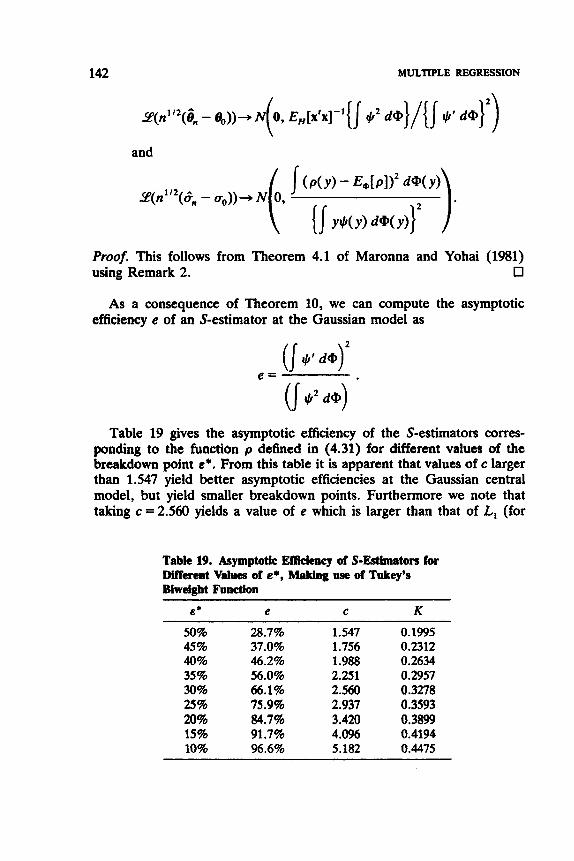
142 MULTIPLE REGRESSION
and
( P ( Y ) - E*[P1)2 d@(Y)
0 Proof. This follows from Theorem 4.1 of Maronna and Yohai (1981) using Remark 2.
1. (I [J Y+(Y) d @ W }
3(n”2(6n - a,))-* N 0,
As a consequence of Theorem 10, we can compute the asymptotic efficiency e of an S-estimator at the Gaussian model as
Table 19 gives the asymptotic efficiency of the S-estimators corres- ponding to the function p defined in (4.31) for different values of the breakdown point E * . From this table it is apparent that values of c larger than 1.547 yield better asymptotic efficiencies at the Gaussian central model, but yield smaller breakdown points. Furthermore we note that taking c = 2.560 yields a value of e which is larger than that of L, (for
Table 19. Asymptotic Efficiency of S-Estimators for Merent Values of E*, Making use of Tukey’s Biweigbt Function
~~
E L e C K 50% 45% 40% 35% 30% 25% 20% 15% 10%
28.7% 37.0% 46.2% 56.0% 66.1% 75.9% 84.7% 91.7% 96.6%
1.547 1.756 1.988 2.251 2.560 2.937 3.420 4.096 5.182
0.1995 0.2312 0.2634 0.2957 0.3278 0.3593 0.3899 0.4194 0.4475

RELATION WITH PROJECTION PURSUIT 143
which e is about 64%), and gains us a breakdown point of 30%. In practice, we do not recommend the estimators in the table with a breakdown point smaller than 25%. It appears to be better to apply the c = 1.547 estimator because of its high breakdown point. From this first solution, one can then compute a one-step M-estimator or a one-step reweighted least squares in order to make up for the initial low efficiency. Such a two-stage procedure inherits the 50% breakdown point from the first stage and inherits the high asymptotic efficiency from the second. An algorithm for computing S-estimators will be described in Chapter 5 .
5. RELATION WITH PROJECTION PURSUIT
The goal of projection pursuit (PP) procedures is to discover structure in a multivariate data set by projecting these data in a lower-dimensional space. Such techniques were originally proposed by Roy (1953). Kruskal (1969), and Switzer (1970). The name “projection pursuit” itself was coined by Friedman and Tukey (1974), who developed a successful algorithm. The main problem is to find “good” projections, because arbitrary projections are typically not very informative. Friedman and Stuetzle (1982) give some examples of point configurations with strong structure, which possess projections in which no structure is apparent. Therefore, PP tries out many low-dimensional projections of a high- dimensional point cloud in search for a “most interesting” one, by numerically optimizing a certain objective function (which is also called a “projection index”). Some important applications are PP classification (Friedman and Stuetzle 1980), PP regression (Friedman and Stuetzle 1981), robust principal components (Ruymgaart 1981), and PP density estimation (Friedman et al. 1984). A recent survey of the field has been given by Huber (1985). The program MACSPIN (D’ Software 1986) enables us to look at two-dimensional projections in a dynamic way.
Let us now show that there is a relation between robust regression and PP. To see this, consider the (p + 1)-dimensional space of the ( x i , yi), where the last component of x i equals 1 in the case of regression with a constant. In this space, linear models are defined by
for some p-dimensional column vector 8. In order to find a “good” i, we start by projecting the point cloud on the y-axis in the direction orthogon- al to (8, -1)‘ for any vector 8. This means that each ( x i , y i ) is projected onto (0, r i (0) ) , where r i ( 0 ) = y i - xi@. Following Rousseeuw (1984, p.
144 MULTIPLE REGRESSION
874) and Donoho et al. (1985), we measure the “interestingness” of any such projection by its dispersion
where the objective s is scale equivariant
s(Tr,, . . . , rr,) = )T(s(r , , . . . , r,) for all T (5.3)
but not translation invariant. The PP estimate 6 is then obtained by minimization of the projection index (5.2). If s(rl, . . . , r , ) = (C;==, rfln)”*, then this “most interesting” 6 is simply the vector of least squares coefficients. Analogously, s (r , , . . . , r , ) = ,T;-, lr,l ln yields the L, estimator, and minimizing ( Z b , Ir,)91n)1’9 gives the L,-estimators (Gen- tleman 1965, Sposito et al. 1977). Using a very robust s brin s us back to our high-breakdown regression estimators: s = (med, r;)”’ yields the LMS, s = (C;=, (r’),:,/n)”’ yields the LTS, and by putting s equal to a robust M-estimator of scale we obtain S-estimators. Note that the minimization of any s satisfying (5.3) will yield a regression estimator that is regression, scale, and affine equivariant (as discussed in Section 4). So any nice s defines a type of regression estimator; by varying s one obtains an entire class of regression estimators belonging to the PP family. Thus the PP principle extends to cover the linear regression problem and to encompass both classical procedures and high-breakdown methods. This notion is best thought of as “PP Linear Regression,” to distinguish it from Friedman and Stuetzle’s (1981) nonlinear and nonrobust “PP Regression.”
It appears that the only affine equivariant high-breakdown regression estimators known so far (the LMS, the LTS, and S-estimators) are related to PP. (GM-estimators do not have high breakdown, and the repeated median is not affine equivariant.) There is a reason for this apparent relation between high breakdown and PP. Indeed, Donoho, Rousseeuw, and Stahel have found that breakdown properties are deter- mined by behavior near situations of exact fit: These are situations where most of the data lie exactly in a regression hyperplane (see Remark 1 following Theorem 3 of Section 4). Such configurations are precisely those having a projection in which most of the data collapse to a point. In other words, high breakdown appears to depend on an estimator’s behavior in those situations where certain special kinds of projections occur. Since PP can, in principle, be used to search for such projections, the usefulness of PP in synthesizing high-breakdown procedures is not surprising.

OTHER APPROACHES TO ROBUST MULTIPLE REGRESSION 145
Table 20. Schematic Overview of Some Affine Equivariant Regression Techniques
Criterion Method Computation E* ~~
Best linear unbiased LS Explicit 0%
Minimax variance M Iterative 0% Bounded influence GM Iterative, Down to 0%
if p with weights on xi (harder) increases
techniques up to 50% High breakdown LMS, LTS, S Projection pursuit Constant,
Note, however, that PP is not necessarily the only way to obtain high-breakdown equivariant estimators, at least not in multivariate loca- tion where Rousseeuw (1983) gives the example of the minimal volume ellipsoid containing at least half the data. Also, not every PP-based affine equivariant estimator is going to have high breakdown (Fill and John- stone 1984).
The relation of our robust regression estimators with PP also gives a clue to their computational complexity. In principle, all possible projec- tions must be tried out (although the actual algorithm in Chapter 5 can exploit some properties to speed things up). This means that the LMS, the LTS, and S-estimators belong to the highly computer-intensive part of statistics,’ just like PP and the bootstrap, to which the algorithm is also related. In Table 20 we have a schematic overview of criteria in affine equivariant regression.
*6. REGRESSION
OTHER APPROACHES TO ROBUST MULTIPLE
We have seen that the conditions under which the LS criterion is optimal are rarely fulfilled in realistic situations. In order to define more robust regression alternatives, many statisticians have exploited the resistance of the sample median to extreme values. For instance, the L , criterion can be seen as a generalization of the univariate median, because the minimization of Zy=, lyi - 61 defines the median of n observations yi. In the regression problem, the L, estimator is given by
n

146 MULTIPLE REGRESSION
The substitution of the square by the absolute value leads to a considerable gain in robustness. However, in terms of the breakdown point, L, is not really better than LS, because the L, criterion is robust with respect to outliers in the yi but is still vulnerable to leverage points. Moreover, Wilson (1978) showed that the efficiency of the L, estimator decreases when n increases. From a numerical point of view, the minimi- zation in (6.1) amounts to the solution of a linear program:
Minimize 2 (ui + v i ) 0 i - 1
under the constraints P
y, = 2 e,x, + ui - vi , ui 2 0, vi 2 0 . k= 1
Barrodale and Roberts (1974) and Sadovski (1977) described algorithms and presented FORTRAN routines for calculating L, regression coef- ficients.
The minimization of an L, norm (for 1s q s 2) of the residuals has been considered by Gentleman (1%5), Forsythe (1972), and Sposito et al. (1977), who presented an algorithm (with FORTRAN code) for the L, fit of a straight line. Dodge (1984) suggested a regression estimator based on a convex combination of the L, and L, norms, resulting in
r2 Minimize (( 1 - 6) $ + S lril) with 0 5 6 5 1 .
8 1-1
Unfortunately, all these proposals possess a zero breakdown point. In Section 7 of Chapter 2, we listed some estimators for simple
regression which are also based on the median. Some of them have been generalized to multiple regression by means of a “sweep” operator (see Andrews 1974).
The idea behind Theil’s (1950) estimator, which consists of looking at the median of all pairwise slopes (see Section 7 of Chapter 2), has also been the source of extensions and modifications. A recent proposal comes from Oja and Niinimaa (1984). For each subset J = {it, i,, . . . , i,} of { 1,2, . . . , n } containing p indices, they define
6, = 6(i,, i,, . . . , i,) (6.2)
as the parameter vector corresponding to the hyperplane going exactly through the p points (xi,, y,,), . . . , (xip, y ip) . They call these 0, pseudo-

OTHER APPROACHES TO ROBUST MULTIPLE REGRESSION 147
observations, and there are Cf: of them. Their idea is now to compute a multivariate location estimator (in p-’dimensional space) of all these 6,. A certain weighted average of the 0J yields LS, but of course they want to insert a robust multivariate estimator. If one computes
4 = myd (OJj for all j = 1,. . . , p (6.3)
(coordinatewise median over all subsets J ) , then one obtains a regression estimator that fails to be affine equivariant. For simple regression, (6.3) indeed yields the Theil-Sen estimator described in Section 7 of Chapter 2. In order to obtain an affine equivariant regression estimator, one has to apply a multivariate location estimator T which is itself affine equivariant, meaning that
T(z,A + b, . . . , z,A + b) = T(z, , . . . , z,)A + b (6.4)
for any sample {z,, . . . , z,} of p-dimensional row vectors, for any nonsingular square matrix A, and for any p-dimensional vector b. For this purpose they propose to apply the generalized median, an ingenious construction of Oja (1983) which is indeed affine equivariant and will be discussed in Section 1 of Chapter 7. Unfortunately, the computation complexity of this generalized median is enormous (and it would have to be applied to a very large set of 0, vectors!). Even when the coordinate- wise median (6.3) is applied, the Oja-Niinimaa regression estimator needs considerable computation time because of the C,P pseudo-observa- tions. In either case the consideration of all 0, is impossible, so it might be useful to consider a random subpopulation of pseudo-observations.
Let us now consider the breakdown point of this technique. We can only be sure that a pseudo-observation 6, = 9(i l , . . . , i,) is “good” when the p points (x i , , y,,), . . . , (xip, y i ) are all good. If there is a fraction E of outliers in the original data, then we can only be certain of a proportion (1 - E)” of “good” pseudo-observations. Therefore, we must have that
because the best possible breakdown point of a multivariate location estimator is 50%, which means that still 50% of “good” pseudo-observa- tions are needed. Formula (6.5) yields an upper bound on the amount of contamination that is allowed in the original data, namely
&* = 1 - ( f )”” . (6.6)

148 MULTIPLE REGRESSION
For p = 2, one finds again the breakdown point of Theil’s estimator. The value of E* in (6.6) decreases very fast with p, as shown in Table 21.
M-estimators (Huber 1973) marked an important step forward in robust estimation. Much research has been concentrated on constructing functions p and t,h (see Chapter 1) such that the associated M-estimators were as robust as possible on the one hand, but still fairly efficient (in the case of a normal error distribution) on the other hand. Note that LS is also an M-estimator with +( t ) = t and that L, regression corresponds to $(t) = sgn (t). Huber (1964) proposed the following t,h function:
if It1 < b = { ‘b sgn (t) if It1 B b ,
where b is a constant. Actually, in a univariate location setting, this estimator was already constructed by the Dutch astronomer Van de Hulst in 1942 (see van Zwet 1985). Asymptotic properties of this estimator are discussed in Huber (1973). Hampel (1974) defined a function that protects the fit even more against strongly outlying observations, by means of
(0 otherwise,
which is called a three-part redescending M-estimator. Figure 19 shows +-functions of both types. In the literature one can find many more +-functions (see Hampel et al. 1986 for a detailed description).
Of course, it is not sufficient to define new estimators and to study their asymptotic properties. Besides that, one has to develop a method for calculating the estimates. The solution of the system of equations (4.32) corresponding to M=estimates is usually performed by an iterative
Table 21. Value of E* = 1 - (4)”’ for Some Values of p
P &* P &*
1 50% 6 11% 2 29% 7 9% 3 21 % 8 8% 4 16% 9 7% 5 13% 10 7%

OTHER APPROACHES TO ROBUST MULTIPLE REGRESSION 149
I
(a)
Figure 19. (a) Huber-type #-function. ( b ) Hampel-type #-function.
procedure. In each step, one has to estimate the coefficients and the scale simultaneously. However, it is very important to start the iteration with a “good” starting value, that is, an estimate which is already sufficiently robust. Without this precaution, one can easily end up in a local minimum that does not correspond at all to the expected robust solution. Dutter (1977) proposed some algorithms for solving the numerical prob- lems associated with M-estimators. The calculation of GM-estimators or bounded-influence estimators [Chapter 1, equation (2.12)] presents simi- lar problems. Dutter (1983a) described a user-oriented and portable computer program (BLINWDR) for calculating these estimates. Marazzi (1986) developed the subroutine library ROBETH, which computes M-estimators and bounded influence estimators. ROBETH also contains robust tests for linear models (Ronchetti 1982) and a variable selection procedure (see also Ronchetti 1985). The corresponding system control program is called ROBSYS (Marazzi 1987). TROLL (Samarov and Welsch 1982, Peters et al. 1982) is a large interactive system for statistical analysis which also includes the computation of bounded influence regres- sion estimators.
Note that the breakdown point of M- and GM-estimators is quite different. Where E* is again 0% for M-estimators because of their vulnerability to leverage points, it becomes nonzero for GM-estimators (Maronna et al. 1979, Donoho and Huber 1983). For p tending to t ~ , the breakdown point of GM-estimators drops to 0% (a small numerical study was performed by Kamber 1985). Yohai (1985) observes that some

150 MULTIPLE REGRESSION
GM-estimators have very low efficiency in the presence of good leverage points. Exact breakdown points of GM-estimators are computed by Martin et al. (1987).
Another approach to robust regression is based on the ranks of the residuals. In the framework of univariate location, these so-called R- esrimurors are due to Hodges and Lehmann (1963). The idea of using rank statistics has been extended to the domain of multiple regression by Adichie (1%7), Jureckovi (1971), and Jaeckel (1972). The proposal of Jaeckel leads to the following definition: If Ri is the rank of ri = yi - xi@, then the objective is to
R
Minimize 2 u, , (Ri )r i , a i - 1
where the scores function a,,(i) is monotone and satisfies Er=, a,,(i) = 0. Some possibilities for the scores a,(i) are:
Wilcoxon scores: a, ( i ) = i - (n + 1)/2
Van der Waerden scores: a,(i) = @-*( i / ( t t + 1))
median scores: a, ( i ) = sgn (i - (n + 1)/2)
bounded normal scores: a,(i) = min(c, max{@>-'(i/(n + l)), - c } ) . (The latter scores were proposed by Rousseeuw 1979 and Ronchetti 1979.) In the case of regression with intercept, one has to estimate the constant term separately, since the objective function is invariant with respect to the intercept. This can be done by using a robust location estimate of the residuals. An important advantage of R-estimators com- pared to M-estimators is that they are automatically scale equivariant, so they do not depend on a simultaneous scale estimator. Nevertheless, Jureckovl(l977) showed that (under certain conditions) R-estimators are asymptotically equivalent to M-estimators. Heiler and Willers (1979) prove the asymptotic normality of R-estimators under weaker conditions than those imposed by JureckovB. Lecher (1980) developed (and im- plemented) an algorithm for R-estimators, in which the minimization (6.9) is carried out by a direct-search algorithm of Rosenbrock (1960). Cheng and Hettmansperger (1983) proposed an iteratively reweighted least squares algorithm for solving (6.9).
The class of L-estimators also plays a prominent role in robust univariate location. They are based on linear combinations of order statistics, and their popularity rests mainly on their simple computation. Bickel (1973) has proposed a class of one-step L-estimators for regres- sion, which depend on a preliminary estimate of 6.

OTHER APPROACHES TO ROBUST MULTIPLE REGRESSION 15 1
Koenker and Bassett ( 1978) formulated another proposal for L- estimators, making use of analogs of sample quantiles for linear regres- sion. They defined the a-regression quanfile (0 < a < 1) as the solution 6, of
n
Minimize p a ( r i ) , e, ; = I
where if ri 2 0
pa(ri)=[T2-i>ri i f r i=O.
(For a =0.5, one obtains the L, estimator.) Koenke: and Bassett then proposed to compute linear combinations of these 6,. Portnoy (1983) proved some asymptotic properties of these estimators. However, note that their breakdown point is still zero.
Also the trimmed least squares estimators of Ruppert and Carroll (1980) are L-estimators. They are counterparts of trimmed means, which are well-known L-estimators of location. (Note that they are not related to the LTS discussed in Section 4.) Ruppert and Carroll proposed two ways to select observations to be trimmed: one of these uses the concept of regression quantiles, whereas the other employs residuals from a preliminary estimator.
Heiler (1981) and Kuhlmeyer (1983) describe the results of a simula- tion study about M-, L-, and R-estimators for linear regression. The behavior of these classes of estimators for different designs and error distributions was compared. It is important to note that the generated samples were rather small, n I 40 and p 5 3, and that no leverage points were constructed. The conclusions from this study can be summarized as follows: LS is very poor, even for mild deviations from normality. M-estimators with redescending $-function turn out to work quite well. R-estimates with Wilcoxon scores, which have the advantage of being scale equivariant (and of being simple to use because no parameter has to be fixed in advance), are a good alternative. L-estimates achieved less satisfactory results.
The first regression estimator with maximal breakdown point is the repeated median due to Siege1 (1982). Like the proposal of Oja and Niinimaa (1984) discussed above, it is based on all subsets of p points. Any p observations (xil, y i l ) , . . . , (xip, y i ) determine a unique parameter vector, the jth coordinate of which is denoted by g ( i , , . . . , i,). The repeated median is then defined coordinatewise as
4 = med (. . . med (med q( i , , . . . , i,))) . . .) . (6.10) 'I ( i,, - I ' p

152 MULTIPLE REGRESSION
This estimator can be calculated explicitly. The fact that the medians are computed sequentially (instead of one median over all subsets) gives the estimator a 50% breakdown point, in which respect it is vastly superior to the Oja-Niinimaa proposal. (The asymptotic efficiency of the repeated median, as well as its influence function, appear to be unknown as yet.) Unfortunately, two disadvantages remain: the absence of affine equivariance and the large number of subsets. However, the second problem might be avoided by selecting some subsets at random instead of using all C,P of them.
Recently, Yohai (1985) introduced a new improvement toward higher efficiency for high-breakdown estimators like LMS and LTS. He called this new class MM-estimators. (Note that they are not related to the MM-estimators considered in Chapter 9 of Rey 1983.) Yohai's estimators are defined in three stages. In the first stage, a high-breakdown estimate 8* is calculated, such as LMS or LTS. For this purpose, the robust estimator does not need to be efficient. Then, an M-estimate of scale sn with 50% breakdown is computcd on the residuals ri(8*) from the robust fit. Finally, the MM-estimator 8 is defined as any solution of
n
which satisfies
where n
s(e) = X p ( r i ( w , , ) . i = l
The function p must be like those used in the construction of S-estimators in Section 4; in particular, it must satisfy conditions (Sl) and (S2). This implies that + = p' has to be properly redescending: Some possibilities are three-part redescenders (6.8), Tukey's biweight (4.17), or the hyper- bolic tangent + (4.16). The trick is that this p may be quite different from that of the scale estimate s, of the second stage, because the first and the second stage must achieve the high breakdown point whereas the third stage is allowed to aim for a high efficiency. Indeed, Yohai showed that MM-estimators inherit the 50% breakdown point of the first stage and that they also possess the exact fit property. Moreover, he proved that MM-estimators are highly efficient when the errors are normally distri- buted. In a small numerical study, he showed that they compare favor- ably with GM-estimators.

OTHER APPROACHES TO ROBUST MULTIPLE REGRESSION 153
In the same spirit of combining high breakdown with high efficiency, Yohai and Zamar (1986) consider “7-estimators” defined by
where again p may be different from that of the scale estimate s,, which is applied to the residuals ri (0) . Asymptotically, a 7-estimator behaves like an M-estimator with a p-function that is a weighted average of the two p-functions used in this construction.
Another possibility, which we have not yet investigated, would be to minimize an objective function of the type
[ n i-1 2 r : (e ) ] A [k’S’(e)] , (6.11)
where A denotes the minimum of two numbers, k > 1, and S(0) is a high-breakdown estimator of scale on the residuals rl(e), . . . , rn(0), which is consistent under normality. For instance, S’((e) may be a multiple of med, r : (e ) or (l ln) E t l (r’(0))i :”, or S(e) may @ a suitable M-estimator of scale. It seems that the minimization (over 0) of (6.11) would combine high asymptotic efficiency with a high breakdown point, because most often the first part (LS) would be used at “good” configura- tions whereas the second part protects from “bad” configurations. How- ever, it remains to be verified whether the actual (finite-sample) behavior of this estimator would be good enough to compete with simple but effective methods like the combination of LMS with a one-step im- provement. REMARK. Suppose that we apply a weighted LS with weights given by
1 if Iri/u*l c c 0 otherwise, wi =
where ri is the LMS residual of yi, and u* is the corresponding LMS scale estimate. For each constant c 2 1, this estimator has breakdown point 50%, whereas for c+ 00 it becomes more and more efficient, and tends to LS. This paradox can be explained by understanding that the breakdown point is only a crude qualitative notion. Indeed, the above estimator with large c will not become unbounded for less than 50% of contamination, but it will not be very good either. [The same is true for the univariate M-estimator of location (6.7) with large b.] One should not forget that the breakdown point is only one out of several robustness criteria, so a

154 MULTIPLE REGRESSION
high breakdown point alone is not a sufficient condition for a good method. We personally consider a good breakdown point as a necessary condition, because we do not want estimators that can become arbitrarily bad as a result of a small fraction of contamination. Indeed, Murphy’s Law guarantees us that such contamination is bound to occur in practice.
EXERClsEs AND PROBLEMS
S & ~ S 1-3 1. Table 22 was taken from Gray (1985). It deals with 23 single-engine
aircraft built over the years 1947-1979. The dependent variable is cost (in units of $loO,O00), and the explanatory variables are aspect
Tabk 22. Aircraft Data
Aspect Lift-to-Drag Index Ratio Ratio Weight Thrust Cost
1 2 3 4 5 6 7 8 9
10 11 12 13 14 15 16 17 18 19 20 21 22 23
6.3 6.0 5.9 3.0 5 .O 6.3 5.6 3.6 2.0 2.9 2.2 3.9 4.5 4.3 4.0 3.2 4.3 2.4 2.8 3.9 2.8 1.6 3.4
1.7 1.9 1.5 1.2 1.8 2.0 1.6 1.2 1.4 2.3 1.9 2.6 2.0 9.7 2.9 4.3 4.3 2.6 3.7 3.3 3.9 4.1 2.5
8,176 6,699 9,663
12,837 10,205 14,890 13,836 11,628 15,225 18,691 19,350 20,638 12,843 13,384 13,307 29,855 29,277 24,651 28,539 8,085
30,328 46,172 17,836
4,500 3,120 6,300 9,800 4,900 6,500 8,920
14,500 14,800 10,900 16,000 16,000 7,800
17,900 10,500 24,500 30,000 24,500 34,000 8,160
35,800 37,000 19,600
2.76 4.76 8.75 7.78 6.18 9.50 5.14 4.76
16.70 27.68 26.64 13.71 12.31 15.73 13.59 51.90 20.78 29.82 32.78 10.12 27.84
107.10 11.19
Source: Office of Naval Research.
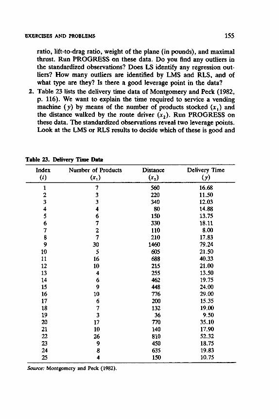
EXERCISES AND PROBLEMS 155
ratio, lift-to-drag ratio, weight of the plane (in pounds), and maximal thrust. Run PROGRESS on these data. Do you find any outliers in the standardized observations? Does LS identify any regression out- liers? How many outliers are identified by LMS and RLS, and of what type are they? Is there a good leverage point in the data?
2. Table 23 lists the delivery time data of Montgomery and Peck (1982, p. 116). We want to explain the time required to service a vending machine (y) by means of the number of products stocked (xl) and the distance walked by the route driver ( x t ) . Run PROGRESS on these data. The standardized observations reveal two leverage points. Look at the LMS or RLS results to decide which of these is good and
Table 23. Delivery Time Data
Index Number of Products Distance Delivery Time
1 7 560 16.68 2 3 220 11.50 3 3 340 12.03 4 4 80 14.88 5 6 150 13.75 6 7 330 18.11 7 2 110 8.00 8 7 210 17.83 9 30 1460 79.24 10 5 605 21.50 11 16 688 40.33 12 10 215 21.00 13 4 255 13.50 14 6 462 19.75 15 9 448 24.00 16 10 776 29.00 17 6 200 15.35 18 7 132 19.00 19 3 36 9.50 20 17 770 35.10 21 10 140 17.90 22 26 810 52.32 23 9 450 18.75 24 8 635 19.83 25 4 150 10.75
(i) ( x , ) (x1) ( Y )
~~ ~ ~ ~ ~~~ ~
Source: Montgomery and Peck (1982).
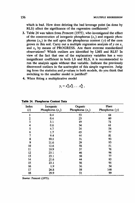
156 MULTIPLE REGRESSION
which is bad. How does deleting the bad leverage point (as done by RLS) affect the significance of the regression coefficients?
3. Table 24 was taken from Prescott (1979, who investigated the effect of the concentration of inorganic phosphorus ( x , ) and organic phos- phorus (xz) in the soil upon the phosphorus content ( y ) of the corn grown in this soil. Carry out a multiple regression analysis of y on x , and x2 by means of PROGRESS. Are there extreme standardized observations? Which outliers are identified by LMS and RLS? In view of the fact that one of the explanatory variables has a very insignificant coefficient in both LS and RLS, it is recommended to run the analysis again without that variable. Indicate the previously discovered outliers in the scatterplot of this simple regression. Judg- ing from the statistics and p-values in both models, do you think that switching to the smaller model is justified?
4. When fitting a multiplicative model
81 s, e yi = xi ,x iz . . . x;; ,
Table 24. Phosphorus Content Data
Index Inorganic Organic Plant (9 Phosphorus ( x , ) Phosphorus ( x z ) Phosphorus ( y)
1 2 3 4 5 6 7 8 9 10 11 12 13 14 15 16 17 18
0.4 0.4 3.1 0.6 4.7 1.7 9.4 10.1 11.6 12.6 10.9 23.1 23.1 21.6 23.1 1.9 26.8 29.9
53 23 19 34 24 65 44 31 29 58 37 46 50 44 56 36 58 51
64 60 71 61 54 77 81 93 93 51 76 96 77 93 95 54 168 99
Source: Prescott (1975).

EXERCISES AND PROBLEMS 157
it is natural to logarithmize the variables. However, in economics it happens that some observations are zero (typically in one of the explanatory variables). It is then customary to put the transformed observation equal to a very negative value. Would you rather use LS or a robust regression method on these transformed data? Why?
5. (Research problem) Is it possible to develop collinearity diagnostics that are not so much affected by outliers?
Sections 4-6
6. Show that the repeated median estimator is regression and scale equivariant, and give a counterexample to show that it is not affine equivariant.
7. (Research problem) It would be interesting to know the asymptotic behavior of the repeated median regression estimator and to obtain its influence function.
8. Show that the variant of the LMS given by formula (4.9) has breakdown point ([(n - p ) / 2 ] + l ) /n .
9. Explain why the breakdown point of the least quantile of squares estimator (4.10) is approximately equal to a. Why doesn’t the breakdown point become higher than 50% when a > i?
10. The L, fit is determined by the narrowest band covering all the data. Consider again some of the simple regression examples of the preceding chapters to illustrate that the L, line is even less robust than LS.
11. Prove that the LWS estimator (4.27) is regression, scale, and affine equivariant, and show that its breakdown point equals the desired value.
12. (Research problem) What is the maximal asymptotic efficiency of an S-estimator defined by means of function p satisfying (Sl), (S2), and (S3) with K = E,[p]?

C H A P T E R 4
The Special Case of One-Dimensional Location
1. LOCATION AS A SPECIAL CASE OF REGRESSION
The estimation of a location and a scale parameter of a single variable can be considered as a particular case of the general regression model, obtained by putting p = 1 and x i = 1 for all i. Then the sample reduces to ( y i ) i = l , , , , . , and the underlying model states
y i = e + ei ,
where 8 is an unknown one-dimensional parameter and e, is normally distributed with mean zero and standard deviation u. In this situation, an estimator T, of 8 is called a univuriute locution estimator, and an estimator S, of u is called a scale estimator.
From the equivariance properties in Section 4 of Chapter 3, which form an integral part of regression estimation, we can derive equivariance and invariance properties for location and scale estimators. First, regres- sion equivariance reduces to so-called locution equivuriunce. Indeed, when a constant u is added to the whole sample, then any reasonable location estimator should be increased by the same amount. More formally, T, is a location (or translation) equivariant estimator if
for any constant u. Also, the scale equivariance of regression estimators can be formulated in the one-dimensional case. Indeed, a location estimator should follow a change of scale of the sample, which is obtained
158
Robust Regression and Outlier Detection Peter J. Rousseeuw, Annick M. Leroy
Copyright 0 1987 John Wiley & Sons, Inc. ISBN: 0-471-85233-3

LOCATION AS A SPECIAL CASE OF REGRESSION 159
by multiplying all the observations by a constant c (not equal to zero). To be precise, a location estimator T,, satisfying
is said to be scale equivariant. A location estimator that is both location and scale equivariant is called ufFne equivariant, because it transforms well when all yi are replaced by cyi + u. (Note that the affine equivariance of regression estimators is different, and it has no counter- part here because we cannot transform any x-variables.)
Let us now look at the behavior of a scale estimator S,, under such transformations. First, adding a constant u to all observations should not change Sn. In other words,
for all u. Any S,, satisfying (1.3) is said to be location invariant. However, S,, does have to follow a change of scale:
that is, S,, is scale equivariant. Note that the absolute value is needed because scale estimators are always positive.
An extensive Monte Carlo study of robust estimators of location has been camed out by Andrews et al. (1972). A recent treatment of one-dimensional estimators can be found in Chapter 2 of Hampel et al. (1986). We will devote some attention to one-dimensional estimation for several reasons. First of all, location estimators can often be used for estimating the constant term of a robust fit when handling a regression model with intercept. Indeed, once g,, . . . , a,,-l are found, it is possible to compute an appropriate as an estimate of location on the sample consisting of all
Furthermore, in any multivariate analysis, it is always useful to be able to study the different variables of the data set in a one-dimensional way before setting up a model. For this purpose, program PROGRESS can list the standardized data. In general, the standardization of a variable is obtained by first subtracting a location estimate of the one-dimensional sample associated with this variable and then by dividing by a scale estimate of the same sample. As such, the standardized data are dimen-
160 THE SPECIAL CASE OF ONE-DIMENSIONAL LOCATION
sionless. Moreover, they possess a zero location and a unit scale (as measured by the same one-dimensional estimators that were used for the standardization). The investigation of these standardized measurements can aid the analyst in discovering some pattern in the distribution of each variable in the data set. For instance, the presence of skewness may be detected. The shape of the observed distribution of a certain variable may then suggest a suitable transformation for this variable, to be applied before carrying out the actual regression.
In PROGRESS, the standardization is performed in a robust way. When there is a constant term in the model, the program starts by subtracting the median of each variable, and then divides this result by the median of absolute deviations from the median (multiplied by the usual correction factor 1 /w1(0.75) = 1.4826). More formally, each ob- servation is transformed to
xii - med xkj
1.4826 med lx, - mfd xkjl ' j = 1 , . . . , p - 1 , (1.5) k zij =
f
and we put zip = x i p = 1 for the intercept term. Moreover, z i ,p+l is the standardized version of the response y i , computed in the same way as in (1.5) but with xij replaced by y i . When there is no intercept term,
X i j 2. . =
'1 1.4826 med IxfjI ' f
j = 1 , . . . , p
and again zi.p+l corresponds to the standardization of the response but with xij replaced by yi in (1.6).
Problems may occur if the denominator of (1.5) or (1.6) equals zero. If this happens, the standardization in (1.5) is substituted by
xii - med xkj
1 " 1.2533 - Ix, - medxkjl
, j = l , . . . , p - 1 (1.7) k 2. . = 11
n f = 1 k
and (1.6) becomes

LOCATION AS A SPECIAL CASE OF REGRESSION 161
where 1.2533 = is another correction factor. (This is because the mean absolute deviation tends to times the standard deviation when the xii are normally distributed.)
A denominator in (1.7) or (1.8) which equals zero would mean that the variable in question is constant over all observations.. When this occurs, the program stops and recommends that the user start the analysis again without that variable, because it does not contain any information.
In Chapter 5 we will explain why standardization is also useful from a numerical point of view.
Finally, standardized observations also provide a simple scheme to diagnose univariate outliers in any single variable (of course, it is supposed here that the standardization has been performed in a robust way). By means of the standardized measurements, one introduces a so-called rejection rule, which consists of identifying all observations with a standardized value larger than some bound. (This is just a special case of looking at the standardized residuals from a robust regression in order to identify regression outliers.) When the target is one-dimensional estimation, one can then estimate location and scale in a classical way on the “cleaned” sample in which the extreme observations are removed. This idea of using rejection as a method of producing a robust estimator has been widely used. Hampel (1985) made a critical study of such rejection rules followed by computing the mean of the remaining data. One of the best rules is X84, corresponding to the removal of observa- tions for which the standardization (1.5) yields an absolute value larger than some bound. This rule leads to a 50% breakdown point. On the other hand, Hampel showed that many classical rejection rules (Barnett and Lewis 1978, Hawkins 1980) yield a low breakdown point, which corresponds to their vulnerability to the masking effect. This is not surprising, because most of these methods are based on classical non- robust estimation.
We will now discuss the one-dimensional versions of some of the regression estimators defined in Chapters 2 and 3. The least squares (LS) estimator reduces to the minimization of
i (Yi - , i = l
which leads to the well-known arithmetic mean. As before, this estimator has a poor performance in the presence of contamination. Therefore, Huber (1964) has lowered the sensitivity of the LS objective function by replacing the square in (1.9) by a suitable function p . This leads to location M-estimators, defined by

162 THE SPECIAL CASE OF ONE-DIMENSIONAL LOCATION
n
Minimize p( y , - 8 ) , (1.10) 0 i = 1
which satisfy the necessary condition n 2 q t ( y , - i ) = O ,
i= 1 (1.11)
where qt is the derivative of p. [Of course (1.10) and (1.11) are not always equivalent.] In order to make an M-estimator scale equivariant, Huber considered the simultaneous estimation of location 6 and scale u by solving the system of equations
(1.12)
These equations have to be solved iteratively. A possible choice of p in (1.10) is the absolute value, yielding the L,-estimator that reduces to the sample median 6 = med, y , . The corresponding scale estimate is obtained by taking x ( y ) = sgn (Iyl - @-' (0.75)) in (1.12), leading to the normal- ized median absolute deviation 6 = 1.4826 medj [ y j - med, y i l . Huber (1964) himself used the functions
y r - k
y > k - k S y S k (1.13)
and
A simplified variant is the one-step M-estimator (Bickel 1975). It results from applying Newton's iterative algorithm for solving (1.12) just once, with initial estimates T o for location and So for scale. This means that the one-step estimate for 8 equals
so. (1.14)
5 qt'{(yi - T o ) / S o } n i = l
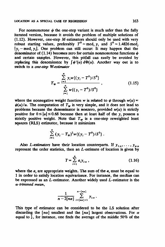
LOCATION AS A SPECIAL CASE OF REGRESSION 163
For nonmonotone t+h the one-step variant is much safer than the fully iterated version, because it avoids the problem of multiple solutions of (1.12). However, one-step M-estimators should only be used with very robust starting values, preferably To = med, y i and So = 1.4826 medj Iy, -medi yi l . One problem can still occur: It may happen that the denominator of (1.14) becomes zero for certain nonmmotone functions # and certain samples. However, this pitfall can easily be avoided by replacing this &nominator by J#'(u)d@(u). Another way out is to switch to a one-step W-estimator
2 y , w { ( y , - T O ) / S O ) T, = (1.15)
2 w { ( y , - T o ) / S o ) i= 1
where the nonnegative weight function w is related to # through w(u) = $(u)/u. The computation of T, is very simple, and it does not lead to problems because the denominator is nonzero, provided w(u) is strictly positive for 0 s 1.1 50.68 because then at least half of the y i possess a strictly positive weight. Note that T, is a one-step reweighted least squares (RLS) estimator, because it minimizes
n
Also L-estimators have their location counterparts. If y l , , , . . . , y,,, represent the order statistics, then an L-estimate of location is given by
n
i= 1 (1.16)
where the ai are appropriate weights. The sum of the ai must be equal to 1 in order to satisfy location equivariance. For instance, the median can be expressed as an L-estimator. Another widely used L-estimator is the a -trimmed mean,
n - [ n u ] 1 2 yi:n * n - 2[nal i = [ n u ] + l
This type of estimator can be considered to be the LS solution after discarding the [na] smallest and the [na] largest observations. For a equal to ), for instance, one finds the average of the middle 50% of the

164 THE SPECIAL CASE OF ONE-DIMENSIONAL LOCATION
order statistics, which is sometimes referred to as the midmean. L- estimators have been investigated by, among others, Bickel and Hodges (1%7), Dixon and Tukey (1968), Jaeckel (1971), Helmers (1980), and Serfling ( 1980).
An R-estimate of location is derived from a rank test statistic in the following way. Consider on the one hand the original sample { y l , . . . , y,} and on the other hand the sample (2T - y , , . . . , 2T - y.} which is obtained by reflecting each y i with respect to some T. Let Ri be the rank of the observation yi in the combined sample. Then an R- estimator of location is defined as the value T, that makes the expression
(1.17)
as close to zero as possible, where J is a scores function satisfying si J ( t ) = 0. This means that the rank test based on the statistic (1.17) sees no shift between the true and the reflected sample. The first such construction made use of the Wilcoxon or Mann-Whitney test given by J ( t ) = t - f , leading to the Hodges-Lehmann (1963) estimator:
Yi + Yj T = med -.
t s i c j s n 2 (1.18)
This estimator equals the median of all pairwise means of the sample, which is analogous to the slope estimator of Sen in the case of simple regression [Chapter 2, equation (7.2)]. By means of the reasoning in formula (7.3) of Chapter 2, we find that its breakdown point is E* = 1 - (4)”’ =0.293.
An estimator that is also worth noting in the framework of robustness is the shorth. This estimator is defined as the arithmetic mean of the shortest subsample with half of the observations. The shorth was intro- duced in the Princeton Robustness Study. Below, we shall see the resemblance between the shorth and the least median of squares (LMS) location estimator. We will also discuss the least trimmed squares (LTS) estimator.
2. THE LMS AND THE LTS IN ONE DIMENSION
In one-dimensional location, the LMS reduces to
Minimize med ( y i - 6)* . e I

THE LMS AND THE LTS IN ONE DIMENSION 165
Before we investigate the properties of this estimator, we will first compare it with some well-known univariate estimators on a real data set. In Rosner (1977) we found a sample containing 10 monthly diastolic blood pressure measurements:
90,93,86,92,95,83,75,40,88,80, (2.2)
which are plotted in Figure 1. A glance at these measurements reveals that 40 stands out compared to the other values.
Figure 1 also contains some location estimates applied to this sample. The arithmetic mean, 82.2, is attracted by the outlier. On the other hand, the robust estimates range from 86.9 to 90.5. Indeed, the sample median equals 87.0, the LMS estimate is 90.5, and the reweighted mean (1.15) with weights based on the LMS becomes 86.9. If the outlier were to move even further away, none of these robust estimates would change any more.
It is striking that the LMS location estimate does not stand in the center of the “good” observations but rather in a position where the points lie very close together. The reason for this phenomenon is that this sample is not symmetric. The LMS looks for a concentration in the sample, which means that it might be considered as some kind of mode estimator. In order to illustrate this, we have sketched a possible underly- ing distribution from which this sample might have been drawn, judging from the observations. This density looks skewed, with the mode situated at the right-hand side in the neighborhood of the LMS location estimate. For such asymmetric samples the LMS lies closer to the mode than do the mean and the median. In fact, a classical measure for skewness is the ratio
mean - mode scale estimate ’
0 -3
I
Mean RLS Med LMS
Feure 1. Rosner data: (above) Ten one-dimensional measurements; (below) some location estimates: Mean, arithmetic mean; Med, median; LMS, least median of squares estimator; RLS, reweighted mean with weights based on the LMS.

166 THE SPECXAL CASE OF ONE-DIMENSIONAL LOCATION
which becomes zero for symmetric situations, positive for skewed den- sities with their tail to the right, and negative if the tail is to the left.
It is important to note that this different behavior of the LMS does not only show up when the sampling distribution is actually skewed, but even when it is symmetric, because experience has taught us that:
Small samples drawn from a symmetric distribution tend to look asymmetric.
This explains the larger variability of mode estimators (such as the LMS). Note that we do not claim that the LMS would be particularly good for
one-dimensional location, and indeed there are many robust estimators with smaller variability in this situation, such as the sample median. However, most of these competitors do not generalize appropriately to multiple regression (such as the usual L , estimator, which is very vulner- able to leverage points). The main motivation for the LMS (and its relatives) comes from the affine equivariant high-breakdown multiple regression setting, where it is not so easy to construct good tools.
Let us now compare the behavior of the objective function of the LMS and the LS on the one-dimensional data set of Rosner. In Figure 2, the dashed line represents the LS objective Zy=, ( y , - t)’ as a function of t, whereas the solid line corresponds to the function med, ( y i - t)’, where { y, , . . . , ylo} is the sample (2.2). The LMS objective function attains its minimum in some T, which equals 90.5 for this sample. The resulting med, ( y i - T)’ is denoted by m:. The LS objective function attains its minimum more to the left, that is, closer to the outlying value 40. The values T- mr and T + mT are also indicated cn the horizontal axis containing the measurements. Since mr equals 4.5, this interval ranges from 86 to 95. Both of these boundary values exactly coincide with an observation. Moreover, it appears that this interval contains half of the sample. These properties are generally true, as stated in Theorem 1 below. We will, however, first show that there exists a solution to (2.1).
Lemma 1. For any univariate sample { y l , y 2 , . . . , y , } , there exists a solution to (2.1).
Proof. Since the convex hull of the sample is compact and the objective function med, ( y i - t)‘ is continuous in t. it follows immediately that there exists a minimum. 0
Theorem 1. If mf : = med, ( yi - T)’ equals min, medi( y i - e)?, then both T - mT and T + mT are observations in the sample { Y I ? Y z . . . . 1 Y , , ) .

THE LMS AND THE LTS IN ONE DIMENSION 167
FEgure 2. Plot of the objective function corresponding to the LS (dashed line) and the LMS (solid line) for the same data set as in Figure 1. These data are also indicated below the plot, which shows that T - mT and T + m, are observed values.
Proof. (a) First suppose that n is odd, with n = 2k - 1. Then the median is reached by the kth squared residual r::@. A residual is the difference between a sample point and the location estimate. Therefore, at least one of the points T - m, or T + mT is an observation in the sample. Without loss of generality, suppose that T + m , is and T - m , is not. There exists a partition of the r;:n in three parts:
2 (k - 1) squared residuals that are sm, ,
1 squared residual that is =m+, and
(k - 1) squared residuals that are Zm, . 2
Suppose yj , , is the smallest observation that is larger than T - m, (choose one if there are several), and define T’ = { ( ( T + m,) + y,,,) and m” = f ( l ( T + m,) - Y ~ : ~ I ) * . It is clear that mr2 < mi. Then there exists a partition of the new residuals (r:)’ = ( yi - T’)2 into

168 THE SPECIAL CASE OF ONE-DIMENSIONAL LOCATlON
(k - 2) squared residuals I m“
(corresponding to the same points as before, except y j z n ) ,
2 squared residuals = m’2
(corresponding to y j , , and T + m7), and
(k - 1) squared residuals 2 m”
(corresponding to the same points as before).
Finally, med, (r:)2 = m” < mi, a contradiction.
denoted by r l z n I * * - 5 rn :n , then ( b ) Suppose that n i s even, with n = 2k. If the ordered squares are
2 2
2 2 mT = ( r k : n + r2k+l:n)/2 *
There is a artition of the squared residuals into (k - 1) squares 5 2 r iZn itself, t k + l : n itself, and (k - 1) squares Zrk+l:n.
If T + mT is an observation and T - mr is not (or conversely), then mi is a squared residual and one can repeat the reasoning of case (a), yielding the desired contradiction. Now su pose that neither T + mT nor T - mT are observations, which implies rk:n < because otherwise r k : n - mT = r k + l : n . Therefore, at least r k + l z n > 0. Now two situations can occur :
4 2 - 2 2 2
(6.1) First Situation: Assume that r i : n = 0. In that case, T coincides with exactly k observations, the nearest other observation (call it y,) being at a distance d = I r ( k + l : n . Putting T’ = (T + y j ) / 2 , however, we find
med ( y , - TO2 = ${( $d)’ + ( = i d 2 < i d 2 = m; ,
a contradiction.
(6 .2 ) Second Situation: Assume that > 0. Denote by y j some observation corresponding to r i : n and by y, some observation correspond- ing to T ~ + , : ~ . If the observations leading to r i : n and r i+ l :n are all larger than Tor a11 smaller than T, one can again repeat the reasoning of case (a). Therefore, one may assume without loss of generality that y j < T < y,. Putting T’ = ( y j + y,) /2, we find
med ( y , - T’)’ = $ { ( y j - T’)2 + ( y , - TI)’} < ;{( y j - T)’ + ( y , - T)’}
2

THE LMS AND THE LTS IN ONE DIMENSION 169
because the function g(t) = (a - t)* + (b - t)* attains its unique minimum 0 at t = (a + b ) / 2 .
Theorem 1 makes it easy to compute the LMS in the location case. One only has to determine the shortest half of the sample. This is done by finding the smallest of the differences
where h = [ n / 2 ] + 1 and y,,, s - - - s ynzn are the ordered observations. The corresponding subsample containing h observations is then called the shortest half because of all the possible subsets with h elements it possesses the shortest range. Then using Theorem 1, T simply equals the midpoint of this shortest interval. (In case there are several shortest halves, which happens with probability zero when the distribution is continuous, one could take the average of their midpoints.) This reminds us of the shorth, where the mean of all observations in the shortest half is taken.
Let us now illustrate the LMS estimate on the sample in (2.2). We first order the observations as follows:
40 75 80 83 86 88 90 92 93 95

170 THE SPECIAL CASE OF ONE-DIMENSIONAL LOCATION
The horizontal lines indicate the halves of the sample. We now consider the differences defined in (2.4), yielding the values 48, 15, 12, 10, 9. The smallest of them corresponds to the distance between 86 and 95. Finally, the midpoint of this interval, namely 90.5, is the LMS estimate of location. Note that the presence of the aberrant value 40 does not affect this result.
REMARK. Note that in the special case of n = 3 the LMS coincides with the mean of the closest pair, Lieblein (1952) investigated the properties of this estimator but concluded that it is not very satisfactory because in such small samples it often happens that two points are very close to each other by chance, making the third one look like an outlier, even when the observations come from a Gaussian distribution. Stefanski and Meredith (1986) recently gave an example in which the mean of the closest pair performs better than the sample median.
We are now in a position to explain why we have considered the median of the squared residuals in (2.1), instead of the median of the absolute residuals, corresponding to
Minimize med I y, - 61 6 1
It turns out that Theorem 1 no longer holds for the latter estimator when n is even. Indeed, consider the sample {1,3,4,6,7,10}. The LMS solution is unique and equals T = 5 with mT = 2. On the other hand, all values of T between 4.5 and 5.5 minimize (2.5) with med, l y i - TI = 2, yielding counterexamples to Theorem 1. Therefore the square in (2.1) is not superfluous. In the general multiple regression model with intercept term (and thus also in the case of location), the following theorem holds.
Theorem 2. Each solution of
Minimize med ( y i - xi,, i1 - - - . - ~ ~ , ~ - ~ 6 ~ - ~ - 4)’ (2.6) e
is a solution of
Minimize e med ly , - ~ , , , 6 ~ - * - - x i , p - l & - l - 6pI * (2.7)
case, med, rt equals the kth squared residual T i z n , where riZn I - - - I rnZn 2 Proof. (a) The implication is obvious when n is odd, n = 2k - 1. In that
are the ordered squared residuals. Since T i Z n = (lrlk:n)’, it follows that rned, (rf) = (rned, Iril)’.

THE LMS AND THE LTS IN ONE DIMENSION 171
(b) When n is even, n can be written as 2k. Let T be a solution to (2.6) and put rn:=(r;:,+ r k + l : n ) / 2 = min,med,(r?). From the proof of Theorem 1, it follows that r;,. = mT = rk+l:n, so
2
2 2
med l r i l = l ( l 4 k : n + I r l k + 1 : n ) = mT
Now suppose that T would not minimize med, Iril. Then there would exist a T' such that
med Ir:\ = mT. < mT .
Repeating case (b) of the proof of Theorem 1, replacing rf by Iril, one can show that there exists a T" such that med, I mr, and lr"lk:n = I r"ik+ Therefore,
1
m?d(<)* = f ( ( j t 2 ) k : n + ( j f 2 ) k + l : n )
I a(mi, + mi,) = m i , < mi ,
which is a contradiction. 0
Let us now look at the LTS estimator in the univariate case, given by
h
where h = [n /2] + 1 and (r2)i:n are the ordered squared residuals.
the following n - h + 1 subsamples: In order to determine the LTS location estimate one has to consider
{ Y 1 : n , - * * 7 Yh:n), { Y 2 : n , * * * 9 yh+l:n}, * ' 7 { Y n - h + l : n t . * ' 9 Y n : n } . (2'9)
Each of these subsamples contains h observations, so we call it a (contiguous) half. For each half, one calculates the mean
and the corresponding sum of squares

172 THE SPECIAL CASE OF ONE-DIMENSIONAL LOCATION
The LTS solution then corresponds to the mean Y ( j ) with the smallest associated sum of squares SQ"!
Proceeding in this way, one has to go twice through the observations of each half. The number of operations can be drastically reduced by using the mean of the preceding half. This means that the mean of the jth half ( j > 1) is determined by the recursive formula
making use of the mean of the ( j - 1)th half. (It is even better to update hf"' in order to avoid rounding errors caused by successive division and multiplication by the factor h.) The sum of squares can also be calculated in a recursive way, namely
Applying this algorithm to the sample (2.2), one finds the value 90.67 for the LTS location estimator, which corresponds to the mean of the half
The least winsorized squares (LWS) estimator in the case of location is { Y S : l O , - - * 7 Y l O l O h
defined by
(2.10)
with h=[n/2]+1. As for the LMS and the LTS, the LWS location estimate can be calculated explicitly.
Lemma 2. The LWS location estimate is given by the midpoint of the contiguous half which leads to the lowest objective function value in (2.10).
Proof. It is obvious that the selected half has to consist of successive observations, since if there were gaps, then one could make the objective

M E LMS AND THE LTS IN ONE DIMENSION 173
function smaller by moving observations. We will now show that the LWS estimate (denoted by T) corresponds to the midpoint of this half. If T < ( y i : n + ~ ~ + , , - , : ~ ) / 2 , then the largest squared residual comes from the observation y i + h - l : n . We are minimizing the sum of n squared residuals, so the objective function will decrease when T is moved in the direction of T', the mean of these n points (in which y i+h- l :n is counted n - h + 1 times):
T' = Y i : n + * + Y i + h - l : n + (n - h)Yi+h-I:n n
- - yi:n + * * * + yi+,t-z:n + ( n - h + l ) Y i + h - l : n
n
If n is even, then n - h + 1 = h - 1 = nl2 , so
( h - 1 ) Y i : n + ( h - l ) Y i + h - , : n - - Y i : n + Y i + h - l : n
2 T ' z
n
If n is odd, it holds that n = 2h - 1 so that
Y i : n + Y i + h - l : n
2 L
In both cases we find T' 2 ( y i : n + ~ ~ + ~ - ~ : , ) / 2 , a contradiction. In an analogous way, one can contradict T > ( y i :n + y i + h - l : n ) 12. Consequent-
0 ly, the LWS estimate equals the midpoint of a half.
However, the selected half is not necessarily the shortest half as in the case of the LMS estimator. Take, for instance, the sample (0, 0, 2, 2 , 3 + E , 4 + 2.9) with E > 0. The midpoint of the shortest half (0, 0 , 2 , 2 } equals 1 and yields the value 6 for the LWS objective function, whereas the midpoint of the half { 2 , 2 , 3 + E , 4 + 2 ~ } is 3 + E , which produces the value 5(1+ E)'. It is possible to make5(1+ E)' smaller than 6, for small values of E. Similar examples with odd sample size can also be con- structed, such as (0, 0, 2 , 2 , 3 + E , 4 + 2 ~ , 4 + 2 e } for n = 7 . But still, Lemma 2 shows that the LWS is more similar to the LMS than to the LTS, and it will often be equal to the LMS. Indeed, for the Rosner data (2 .2) the LWS estimate equals the LMS estimate.

174 THE SPECIAL CASE OF ONE-DIMENSIONAL LOCATION
We will now discuss the S-estimators of location. In Chapter 3, equations (4.28)-(4.30) defined this class of estimators for the multiple regression model. This definition is still valid in the case of location, keeping in mind that 8 becomes one-dimensional and that ri simply equals y i - 8 . Therefore, we want to
Minimize s( y, - 8, . . . , y , - 0 ) , (2.11) 0
where the dispersion s (r l , . . . , r , ) is defined as the solution of
1 " - 2 p ( r i / s ) = K . n i = l
The last formula defines an M-estimator of scale, which is usually computed in an iterative way starting with the initial value
So = 1.4826med l r i l . I
Because of constraints on computation time, it may be appropriate to use a simple and fast approximation of the objective function, such as the one-step estimate
(2.12)
where p may, for instance, be given by formula (4.31) of Chapter 3. One then makes use of a numerical algorithm for minimizing S' as a function of 1
3. USE OF THE PROGRAM PROGRESS
The same program that we used in the previous chapters for the computation of robust regression coefficients also provides one-dirnen- sional estimators. The output of PROGRESS contains the arithmetic mean, the LMS, and the reweighted mean based on the LMS. For each of these location estimates, a corresponding scale estimate is given. As in the multivariate case, the output includes tables of residuals and index plots (at least if the print and plot options are chosen accordingly).
There are two ways to tell PROGRESS to execute the one-dimension- a1 algorithm. The first is to answer 1 to the question

USE OF THE PROGRAM PROGRESS 175
TBE PROBLEM IS REDUCED TO ESTIMATING A LOCATION PARAMETER.
On the other hand, when you want to study the location and scale of a certain variable in a larger data set, you must choose that variable as your response variable, and then the question
must be answered with 0. Once PROGRESS is executing the one-dimensional case, some of the
questions of the interactive part (as discussed in the case of more general regression) no longer apply, so they are not asked. Also, it does not matter whether you have answered YES or NO to the question about whether the regression model contains a constant term.
We will illustrate the program on a one-dimensional data set published by Barnett and Lewis (1978). The sample consists of the numbers
3,4,7,8,10,949,951. (3.1)
Barnett and Lewis used this example for discussing the masking effect when applying outlier tests based on statistics of the type
Y n : n - Y n - l : n
Y n : n - Y 1:n
For the data (3.1), this test does not detect y n Z n as an outlier because of the small difference between y n q I Z n and y,,:,. Repeated application of this single outlier test will not remedy the problem. Also, nonrobust es- timators of location and scale will be strongly affected by these aberrant values. The output of PROGRESS, which is printed below, confirms the need for a robust estimator. Indeed, it appears that the mean (=276) is pulled in the direction of the outliers. Moreover, the standard deviation S is inflated accordingly. The standardized residuals are displayed in an index plot. Note that both outliers fall inside the classical tolerance band, because 6 has exploded! In contrast, the LMS and the LMS-reweighted mean both diagnose the values 949 and 951 as outliers in a very convincing way and provide good estimates for the majority of the data.

176 THE SPECIAL CASE OF ONE-DIMENSIONAL LOCATION
. . . . . . . . . . . . . . . . . . . . . . . . . . . . . . . . . . * ROBUST ESTIMTIOX Of LOCATIOX. % . . . . . . . . . . . . . . . . . . . . . . . . . . . . . . . . . . lWHBEROFCASES- 7
DATA BET = OSS-DI1IHS810SAL DATA 8PT OF BAl.BTT A I D LBVI8 (lP76>
THE DESIRED OUTPUT IS LAROE.
A S ISDEX PLOT VILL BE DRAW. THE OBSERVATIOBS ARE:
1 3.0000 2 4.0000 3 7.0000 4 8.0000 5 10.0000 6 949.0000 7 951.0000
TAE MEDIAB * 8 .0000 THE HAD (+ 1.4826) - 5.9304 ***************a******a******:*******t********************x**************aa*
THE MEAS = 276.0000 STAUDARD DEVIATIOU = 460.4360
OBSERVED RESIDUAL BO REWSC I
3.00000 4.00000 7.00000 a. 00000 10.00000 949.00000 951.00000
1 8 5 7
-.69 -.Be -.sa -.SO -.58 1.46 1.47
Om-DIWUSIOXAL DATA SET OF BARHETT AUD LEVIS (1978)
STAW. RESIDUAL 2.5
0 . 0
1
I I
i I I I I 1
-2.5 tt++ttt++++tt+++t++++t+++tt+++t+++tt+t+tt++++ttt++t++tt 1 I I-t----+----+----+----+----+----+----+----t----+----t-I
1 7 IUDEX OF THE OBSERVATIOX
. . . . . . . . . . . . . . . . . . . . . . . . . . . . . . . . . . . . . . . . . . . . . . . . . . . . . . . . . . . . . . . . . . . . . . . . . . . . . .

USE OF THE PROGRAM PROGRESS 177
I LHS 5.5000 CORRESPOBDIEG SCALE = 6.7952
OESERVED RESIDUAL IVO RES/SC Y
3.00000 4.00000 7.00000 8.00000 10.00000 949.00000 951.00000
-2.50000 1 -.37 -1.50000 2 -.22 1.50000 3 .22 2.50000 4 .37 4.50000 5 .66
943.50000 6 138.85 945.50000 7 139.14
Om-DIHFXSIOYAL DATA SET OF BABWTT A S D LEVIS (1978) - - - L E A S T N E D I A ~ O F S Q U A R E S - - -
+
.............................................................................. REVEIGHTIIG USIIC THE WEIGHTS BASED OX THE LlCS. ............................................... VEIGHTED NEAX I 6.4000 WEIGHTED STASD. DEV. = 2.6810
THERE ABE 5 W I m VITH IDY-ZERO VEIGHT. AVERAGE WEIGHT I .714288
OBSERVED RESIDUAL XO R W S C VBIGHT I
3.00000 -3.40000 1 -1.18 1.0 4.00000 -2.40000 2 -.83 1.0 7.00000 .soooo 3 .21 1.0 8.00000 1.60000 4 .56 1.0 10.00000 3.60000 5 1.25 1.0 949.00000 942.60000 6 327.18 . O 951.00000 944.60000 7 327.88 . O

178 THE SPECIAL CASE OF ONE-DIMENSIONAL LOCATION
OEE-DIXE1161011AL DATA SET OF BAR.ETT AED LEVIS (1978) - - - R E V E I G H T E D L S ( B A S E D 0 1 L H S > - - -
1 I .3279E+03 t 1 1 t
I I I I I I I I * t
I I I
I I I I I t +
I I I I I I
I I t t
I I 1 I 1
I I I t t
I I I I I
I I I t
I I I 1 I I I I t + I I I I
1 I I
I t + I I I 1
2.5 Itt~tttttttttt+tt+ttttt~ttttttttt+ttttttttttttttttttttl 0 . 0 I-l-------l-------l-------l--------l------------------I -2.5 ttttt++tttttttttttttttt*ttttttt**t+ttttttttttttt+tttttt
I -_-- t ---- * -__- t _--_ t ---- .+ ---- t ---- t ---- t _--- t ---- +-I IEDEX OF Ti%% OBSERVATIOE
GTABD. RESIDUAL 1-+----+----+----t----+----+----+----+----t----t----t-I
1 7
................................................................................
REMARK. The scale estimate u* associated with the LMS location estimate is defined as in the regression case [see (3.10) in Chapter 21. This o* is itself a high-breakdown robust estimator, some properties of which are discussed by Rousseeuw and Leroy (1987).
*4. ASYMPTOTIC PROPERTIES
We have seen that the one-dimensional LMS resembles the “shorth” discussed in the Princeton Robustness Study (Andrews et al. 1972; see also Shorack and Wellner 1986, pp. 767-771). Like the shorth, the LMS also converges as n-’13, which is abnormally slow. On the other hand, both the LTS and S-estimators are shown to converge at the usual n-”’ rate. However, the LMS is more easily computable than either the LTS or S-estimators. The fact that the LMS converges like n-I13 does not trouble us very much, because we consider it mainly as a data analytic

ASYMPTOTIC PROPERTIES 179
tool, which may be followed by a one-step improvement to obtain higher efficiency (if necessary).
Theorem 3. If the observations y,, . . . , y,, are i.i.d. according to F( y - (I), where F has a symmetric and strongly unimodal density f, then the distribution of the LMS estimator T,, converges weakly as
2(t1"~(~,, - e))+ q c ~ ) ,
where C = (f( q)f'( q)2/2)-''3, q = F-'(0.75); and T is the random time s for which W(s)+ s attains its minimum, where W(s) is a standard two-sided Brownian motion originating from zero.
Proof. This result is obtained by repeating parts 1, 2, and 3 of the heuristic reasoning of Andrews et al. (1972, p. 51). Using their notation, putting a = 0.25 yields the constant
A = {Gf (F- ' (O .75) ) / - f'(F-'(0.75))}2'3 .
The remaining part of the calculation is slightly adapted. If t^ is the minimizing value of t , then the main asymptotic variability of T,, is given
$[F,'(t^+ 0.75) + F,'(t^+ 0.25)] = t^(F-')'(0.75)
by
= t^/f(F-'(0.75)),
where t ~ " ~ t ^ behaves asymptotically like AT. By putting C:= A / 0 f(F-'(0.75)), we obtain the desired result.
REMARK. In Section 4 of Chapter 3 we considered variants of the LMS where it is not the median of the squared residuals that is minimized, but instead a larger quantile (r'),,:,, (or equivalently Irl,,:,,). One puts h approximately equal to n( 1 - a), where 0 < a < 50%, so we must look for the shortest subsample containing a fraction of (1 - a) of the observa- tions. In this case, Theorem 3 is still valid, but with q = F-'(l- a/2).
The minimization of W(s) + s2 (or equivalently, the maximization of W(s) -s2) occurs in many places in probability and statistics. For in- stance, the distribution of Chernoffs (1964) mode estimator (based on an interval of fixed length, shifted along the line to a position where it contains the highest number of observations) also converges (after stan-
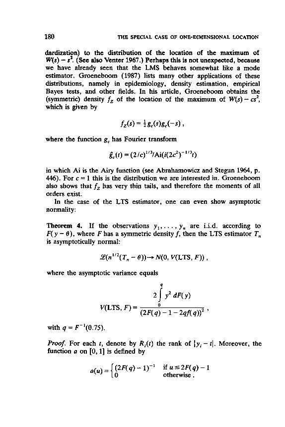
180 THE SPECIAL CASE OF ONE-DIMENSIONAL LOCATION
dardization) to the distribution of the location of the maximum of W(s) - s2. (See also Venter 1967.) Perhaps this is not unexpected, because we have already seen that the LMS behaves somewhat like a mode estimator. Groeneboom (1987) lists many other applications of these distributions, namely in epidemiology, density estimation, empirical Bayes tests, and other fields. In his article, Groeneboom obtains the (symmetric) density fi of the location of the maximum of W(s)-cs2, which is given by
where the function g, has Fourier transform
&( t) = (2 /c)Il3/Ai( i( 2~’)- ‘13t)
in which Ai is the Airy function (see Abrahamowicz and Stegun 1964, p. 446). For c = 1 this is the distribution we are interested in. Groeneboom also shows that fz has very thin tails, and therefore the moments of all orders exist.
In the case of the LTS estimator, one can even show asymptotic normality:
Theorem 4. If the observations y,, . . . , y, are i.i.d. according to F( y - O ) , where F has a symmetric density f, then the LTS estimator T, is asymptotically normal:
.qd’*(~, - e))+ ~ ( o , ~(LTS, F)) ,
where the asymptotic variance equals
with q = F-’(0.75).
Proof. For each t, denote by Ri( t ) the rank of I y i - tl . Moreover, the function Q on [0,1] is defined by
( 2 ~ ( 4) - i ) - I a(u) = if u s 2F( q ) - 1 otherwise.

ASYMPTOTIC PROPERTIES 181
Then the LTS estimator corresponds to the minimization of I$, a(R, (T, ) /n) (y , - t)’. Because there exist only a finite number of points t where Ri(t) changes, we may assume without loss of generality that all Ri(t) are locally constant around the solution t = T,. On this neighborhood (T,, - 6, T,, + 6 ) we put
1 a, = a(&( T,) /n) and S, = - a(Ri( T,,) /n)y , .
n i = l
Now T,, minimizes ,Z7=l ai ( (y i - S,,) + (S, - t))2 = Ey=l ai (y i - S,,)’ + ,Zy=l a,(S, - t)’ for all t in (T,, - 6, T,, + 6 ) . Differentiating this expres- sion with respect to t at T,,, we find that T, = s,,. Therefore T,, is a solution of the equation
1 ” n - z a(Ri( t ) /n)yi = t .
Estimators satisfying this equation with this function a are due to Gnanadesikan and Kettenring (1972). Their asymptotic normality was
0 shown by Yohai and Maronna (1976), giving the desired result.
An immediate consequence of this theorem is that the LTS has the same asymptotic behavior at F as the Huber-type “skipped” mean, which is the M-estimator of location corresponding to the +-function
Y i f l v l s q + ( Y ) = { 0 otherwise.
REMARK. In the previous chapter we also discussed variants of the LTS where approximately n( 1 - a) of the squared residuals are used, for 0 < a < 50%. In this case, Theorem 4 and formula (4.1) can still be applied, but with q = F ’ ( 1 - a/2).
The asymptotic normality of S-estimators at the Gaussian model has already been proven in the general regression case in Chapter 3, Theorems 9 and 10. Of course, these results still hold in the special case of location.
At this point it may be noted that the asymptotic normality of both the LTS and S-estimators basically rests on (variants of) the central limit theorem (CLT). Unfortunately, there exists a fairly widespread misun- derstanding about the interpretation of the CLT, leading some people to claim that “robust statistics are not necessary because data are normally distributed by the central limit theorem.” However, the CLT says

Tab
le 1
. So
me
Stat
istic
s on
the
LM
S, L
WS,
LT
S, a
nd M
edia
n E
stim
ator
s, B
ased
on
500
Gen
erat
ed S
ampl
es fo
r E
ach
n
Mea
n of
St
anda
rd D
evia
tion
of
Intc
rqua
rtile
Ran
ge o
f
n LMS
LWS
LTS
Med
LM
S LW
S L
TS
Med
LM
S LW
S LT
S M
ed
10
20
30
40
50
60
80
100
200
300
400
500
600
800
900
loo0
1 100
IMO
1Mo
1400
IM
O
1600
17
00
m
-0.034
0.005
0.039
0.043
0.00
8 0.005
0.011
0.024
-0.002
0.012
0.015
-0.003
-0.006
-0.0
04
-0.008
-0.004
-0.0
09
-0.003
-0.004
-0.002
-0.002
0.001
-0.003
-0.004
-0.026
0.003
0.030
0.041
0.028
0.00
8 0.011
0.015
0.005
0.013
0.014
0.001
-0.003
-0.002
-0.007
-0.004
-0.005
-0.0
02
-0.003
-0.001
-0.005
-0.004
-0.001
O.O
o0
-0.025
0.00
6 0.030
0.043
0.036
0.034
0.017
0.017
0.00
4 0.010
0.003
O.O
o0
-0.006
0.00
7 0.
004
0.00
2 -0.003
0.00
3 0.
002
0.00
3 0.003
0.00
4 0.
002
0.00
2
-0.027
0.012
0.022
0.020
0.016
0.W
0.010
0.010
0.00
7 0.
005
0.00
2 0.001
0.001
0.00
2 0.
002
0.001
0.001
0.001
0.001
0.001
0.001
0.00
2 0.001
0.001
~ ~
~~
0.48
6 0.491
0.495
0.340
0.669
0.643
0.711
0.463
0.416
0.368
0.348
0.323
0.313
0.284
0.275
0.217
0.195
0.173
0.158
0.150
0.130
0.125
0.124
0.121
0.120
0.115
0.111
0.113
0. I10
0.106
0.098
0.428
0.359
0.353
0.329
0.312
0.28
9 0.267
0.210
0.187
0.162
0.151
0.141
0.125
0.118
0.116
0.115
0.113
0.112
0.105
0.102
0.101
0.09
7 0.
089
0.435
0.371
0.374
0.347
0.327
0.30
9 0.285
0.221
0.185
0.161
0.146
0.140
0.122
0.117
0.114
0.110
0.102
0.100
0.093
0.09
2 0.091
0.08
9 0.080
0.255
0.202
0.186
0.165
0.150
0.136
0.122
0.086
0.071
0.061
a053
0.049
0.042
0.039
0.038
0.036
0.034
0.032
0.031
0.031
0.030
0.030
0.027
0.546
0.485
0.459
0.413
0.412
0.385
0.377
0.290
0.28
0 0.234
0.213
0.208
0.183
0.16
9 0.175
0.166
0.167
0.159
0.153
0.145
0.152
0.146
0.130
0.574
0.468
0.487
0.459
0.418
0.387
0.362
0.283
0.265
0.224
0.216
0.191
0.175
0.162
0.157
0.161
0.155
0.153
0.141
0.138
0.141
0.137
0.119
0.60
2 0.517
0.534
0.499
0.437
0.427
0.405
0.314
0.273
0.219
0.201
0.200
0.179
0. I63
0.166
0.158
0.150
0.137
0.132
0.129
0.131
0.122
0.113
0.358
0.282
0.245
0.219
0.202
0.179
0.169
0.118
0.098
0.079
0.073
0.072
0.057
0.054
0.052
0.04
8 0.047
0.043
0.043
0.04
0 0.041
0.041
0.036

BREAKDOWN POINIS AND AVERAGED SENSlTIVlTY CURVES 183
essentially that most estimators are asymptotically normal. For instance, a robust S-estimator applied to Cauchy-distributed observations will be asymptotically normal, but of course this does not imply that the observa- tions themselves would look at all normal!
Let us now compare these asymptotic properties with simulation results. For different values of n, we generated 500 samples { y,, . . . , y,} from the standard normal distribution. On each sample the LMS, the LWS, the LTS, and the median were calculated. Some statistics on these 500 replications are listed in Table 1. The first column contains the average estimate over the 500 replications and shows that all four estimators approach the true value 0 with more accuracy when the sample size n increases. The standard deviation over the 500 replications is contained in the second column. For most values of n, the LMS possesses the largest standard deviation, followed by the LWS, the LTS, and the median. The same can be said for the interquartile range. Judging from the LMS and LTS columns, the difference between n-’13 and n-’” convergence rates does not yet appear to be visible for n up to 2000.
*5. CURVES
BREAKDOWN POINTS AND AVERAGED SENSITIVITY
The breakdown point E* for affine equivariant estimators of location is at most 50%, just as in the case of general regression models. Indeed, if E*
were larger than 50%, then one could build a configuration of outliers which is just a translation image of the “good” data points.
The sample median enjoys a 50% breakdown point. On the other hand, the arithmetic mean breaks down in the presence of one outlying observation and thus has E* = 0%. Theorems 2, 6, and 8 of Chapter 3 stated that the breakdown points of the LMS, the LTS, and S-estimators for regression (with p > 1) reached 50%. The same can be said for their location counterparts.
Theorem 5. At any univariate sample Y = {y,, . . . , y”}, the breakdown point of the LMS estimator equals
E:( T, Y ) = [ (n + 11/21 n 7
which converges to 50% as n+ 03.
Proof. Without loss of generality, let T(Y) = 0. We put M := maxiIyil. Let us first show that e,*(T, Y) s [ (n + 1 ) / 2 ] / n . For this purpose we

184 THE SPECIAL CASE OF ONE-DIMENSIONAL LOCATION
replace [ (n + 1 ) / 2 ] observations of Y by the same number of points, which are all equal to the value y with I y l > M . This new sample Y‘ then contains only h - 1 of the “good” points, where h = [ n / 2 ] + 1. Therefore, each half of Y’ comprises at least one such large value. Consequently, the midpoint of each half becomes arbitrarily large when I yl - 00, which entails that I T( Y’)l- 00. On the other hand, s,*(T, Y) 2 [(n + 1 ) / 2 ] / n . Indeed, construct a
sample Y” where less than [(n + 1)/2] observations are replaced by arbitrary values. Because there are still at least h “good” points present in Y‘, there exists a “good” half with length at most 2 M . Therefore, the length of the shortest half of Y“ is also at most 2 M . Now suppose that I T(Y‘’)( > 2 M . But then all observations in the shortest half around T(Y”) have absolute values strictly larger than M . This is a contradiction because h > [ ( n + 1 ) / 2 ] - 1, which implies that each half contains at least one “good” point, with absolute value s M . To conclude, we have shown
0 that I T(Y’)l I 2M for any such contaminated data set Y’.
Note that we were not able to apply Theorem 2 of Chapter 3 here because its proof rested on the assumption that p > 1. If we insert p = 1 in the old expression for &,*, we do not find the exact value for the location estimator.
The location counterpart of “exact fit” is a configuration where a certain percentage of the observations in the sample are equal. For the LMS, one finds (as a consequence of the preceding theorem) that if at least [ n / 2 ] + 1 of the observations coincide, then the LMS estimate will also be equal to that value, whatever the other observations are.
Theorem 6. At any univariate sample Y = { yl , . . . , y n } , the breakdown point of the LTS estimator equals
which converges to 50% as n + w.
Proof. We retrace the proof of the preceding theorem. For E;(T, Y ) s [ (n + 1 ) / 2 ] / n , it suffices to note that also the mean of each half of Y’ becomes arbitrarily large when IyI- ,m, and the LTS is just one of those. Also, the proof of E:(T, Y) z [ (n + 1 ) / 2 ] / n looks very much the same. Because there are still at least h “good” points present in Y”, it is clear that C:,( Y “ ’ ) ~ : ~ 5 hM’. Therefore, the residuals ry = yi - T ( Y ) must also satisfy C;=l(r”Z)i:n 5 hMZ. Suppose now that IT(Y”)l> (1 + G ) M .

BREAKDOWN POINTS AND AVERAGED SENSITIVITY CURVES 185
But h > [(n + 1)/2] - 1 implies that each half of Y” contains at least one “good” point, with absolute value 5 M, so that
C f = l ( f ’ 2 ) i : n > ((1 + V X ) M - M}’ = hMZ ,
which is a contradiction. To conclude, we have shown that I T( Y”)lI 0 (1 + a ) M for any contaminated data set Y“.
As a consequence, the LTS estimator of location on a sample where at least [n/2] + 1 of the points are equal will yield that value as its estimate, whatever the other observations are.
The same reasoning as in the proofs of Theorems 5 and 6 can be repeated for the LWS estimator of location. Also, for S-estimators we obtain the same breakdown point by applying Lemma 4 of Chapter 3.
We will now show that this breakdown point is indeed the highest possible value for any location equivariant estimator.
Theorem 7. The breakdown point of any location equivariant estimator satisfies
[(n + 11/21 &,*( T, Y) = n
at any sample Y = { y,, . . . , y,). Proof. Put q = n - [(n + 1)/2], which also equals [n/2]. Suppose that the breakdown point is strictly larger than [(n + 1)/2]/n. This would mean that there exists a finite constant b such that T(Y’) lies in the interval [ T(Y) - b, T( Y) + b] for all samples Y’ containing at least q points of Y. Take, for instance,
Y ’ = { Y ~ , - 9 Yq, Yq+l + u , * * . 7 Y n + v ) 9
which satisfies T( Y’) E [ T(Y) - b, T( Y) + b]. However, note that also the contaminated sample
rr= {yl - u,. . . , Y, - u, y q + l , . - . , Y,}
contains at least q points of Y, so that also T(Y”) E [ T(Y) - b, T(Y) + b]. (Indeed, 2q = n if n is even, and 2q = n - 1 if n is odd, so always 2q I n.) However, Y‘ = Y” + u so by location equivariance we find that T(Y’) = T(Y”) + u, and hence
T(Y‘)€ [T(Y) - b + u, T(Y) + b + u].

186 THE SPECIAL CASE OF ONE-DIMENSIONAL LOCATION
But this is a contradiction, because the intersection of [ T( Y) - 6, T(Y) + b] and [ T(Y) - 6 + u, T(Y) + b + u ] is empty for large enough values of u.
To conclude this discussion, we list some location estimators with their breakdown point in Table 2.
Some other robustness concepts can be found in Hampel et al. (1986). Whereas the breakdown point is a global measure of reliability, they also stress the importance of the influence function (IF), which measures the effect of infinitesimal perturbations on the estimator. The IF of an estimator T at a distribution F is given by
T(( 1 - E)F + &Ay) - T(F) &
IF(y; T,F)=l im e-ro
(5.1)
in those points y of the sample space where the limit exists. (Here Ay is the probability distribution that puts all its mass in the point y.) The IF reflects the bias caused by adding a few outliers at the point y, standar- dized by the amount E of contamination. The IF provides a linear approximation of the estimator at such contaminated distributions:
T((1- E)F + &Ay) = T(F) + E IF ( y ; T, F) . ( 5 4
When working with finite samples we do not use T(F) but rather T(F,,), where F,, is the empirical distribution generated by the sample {yi,. . . , y n } . If we replace one observation by an outlier at y, we find
Table 2. Breakdown Points of Some Loeation Estimators
Estimator Breakdown Point (%)
Mean 0 a-Trimmed mean Median Hodges-Lehmann Shorth LMS, LTS, LWS S-estimators
a 50 29 50 50 50

BREAKDOWN POINTS AND AVERAGED SENSITIVITY CURVES 187
and it is even possible to replace a small fraction E = m/n of observations:
The breakdown point E : provides us with a rough upper bound on the fraction of outliers for which such a linear approximation might be useful.
To understand better the difference between the concepts of break- down point and influence function, let us resort to a physical analogy. Figure 3 was taken from a treatise of Galilei (1638) on applied mech- anics. In this work he considered a beam which is fixed at one end, and to which a stone is attached. To clarify the relation with our statistical subject, we denote the weight of the stone by E and the position where it exerts its force by y. Two questions naturally arise, which are still equally important-and nontrivialln contemporary mechanics, First, how heavy does the stone have to be to make the beam break? (In his treatise, Galilei provided a reasoning showing that this breakdown point is propor-
Figure 3. Illustration taken from Galilei (1638). for showing the difference between the concepts of breakdown point and influence function.

188 THE SPECIAL CASE OF ONE-DIMENSIONAL LOCATION
tional to the width of the beam multiplied by the square of its height.) A second question is, how much does the beam bend for smaller weights? The answer to this question came only around 1825, when Navier gave a mathematical formulation of what is known today as Hooke’s law, stating the proportionality of stress and strain. Nowadays one realizes that Hooke’s law is only a first-order approximation: for small weights E , the deformation of the beam is indeed linear in E . The ratio of deformation divided by weight (or, more accurately, the slope of this relation at E = 0) roughly corresponds to Young’s elasticity modulus. Our influence func- tion is just a plot of the elasticity as a function of y, the position of the external force. For small weights, one can predict the effect by means of a linear approximation such as (5.2). However, the actual computations in present-day mechanics have become much more laborious. As soon as the weight E is larger than “infinitesimal,” the deformations inside the beam become much more complex and Hooke’s law is no longer valid. One resorts to systems of differential equations instead, which are solved by computer simulations (the so-called finite element method). These intricate models give a more accurate description of reality and are necessary to compute the breakdown point of complicated structures such as large buildings or bridges. In the same spirit, the study of influence functions of estimators is more and more being complemented by the consideration of breakdown points and simulations.
All estimators possess a breakdown point, but not all of them have an influence function. However, estimators that do are often asymptotically normal:
where the asymptotic variance is related to the IF through
(see Hampel et al. 1986, Section 2.1). Typical examples of this are M-, L-, and R-estimators.
From Theorem 3, we have learned that the LMS converges merely like n . Therefore, its influence function is not well defined. Nevertheless, we find that statistical efficiency is not the most important criterion. As a data analytic tool, the LMS is very satisfactory. Moreover, it is not so difficult to construct variants with higher efficiency, as has already been discussed in Chapter 3 in the general regression case. In order to get some idea of the local robustness properties of the LMS, we resort to a
- 1 1 3

BREAKDOWN POINTS AND AVERAGED SENSITIVITY CURVES 189
finite-sample version of the IF, namely the stylized sensitivity curve SC, (see Andrews et al. 1972). We start with an artificial sample containing n points
{yi , . . . , y,} = {@- ' ( i / (n + I)); i = I, . . . , n} ,
where Q, is the standard normal cumulative distribution function. Then we plot the curve
for y ranging over an interval containing the points y,. By means of this curve we can also compute
1 " n i= i
v, = - c. [SC,(y,)12 .
If the estimator T, is really asymptotically normal, then the sensitivity curve should converge to the influence function as n + 00, and V, to the asymptotic variance. We have investigated SC, and V, for samples as constructed in (5.6). Some LMS sensitivity curves appear in Figure 4. From this plot, we see that for larger sample sizes the upward and downward peaks become thinner and higher. Combining this information with heuristic arguments, one can conclude that the sensitivity curve of the LMS converges to zero, except in -Q,-'(0.75) and 0-'(0.75) where the function tends to -00 and m.
The values of V, for the LMS are contained in Table 3. For increasing n, the associated values of V, are ever-growing numbers, indicating that n Var(T,) does not tend to a finite limit. In contrast, the quantity V, for the median (last column in Table 3) seems to stabilize around 1.57 for large n. This corresponds to the theoretical asymptotic variance because the influence function of the median at the normal is
IF( y; median, Q,) = sgn (y)/(24(0)) ,
from which it follows that
V (median, Q,) = (24(0))-* = 7r/2 = 1.571 . In Theorem 4 we have seen that the LTS converges like n-'", with the
same asymptotic behavior at the normal distribution as the Huber-type

190 THE SPECIAL CASE OF ONE-DIMENSIONAL LOCATION
15 -
10 -
5 -
0
-
-
-
1.5
-5 -
-10 -
-15 -
Figure 4. Stylized sensitivity curves of the LMS location estimator, for different sample Sizes.
skipped mean [see (4.1)]. The influence function of such M-estimators of location at symmetric distributions F is given by
and their asymptotic variance is therefore
(5.10)
For the LTS, this suggests that

BREAKDOWN POINTS AND AVERAGED SENSlTIMn CURVES 191
Table 3. Value of V, for the LMS, LWS, LTS, and Median (for Different n)
n V, for LMS V, for LWS
10 4.213 5.005 20 13.182 6.247 40 14.373 15.759 100 17.738 20.795 300 38.048 23.178 600 54.074 38.340 loo0 71.546 47.591
V, for LTS V, for Median
10.206 1.578 14.702 1.573 14.588 1.571 14.267 1.571 13.545 1.560 13.596 1.566 13.967 1 S69
(5.11)
which can also be rewritten as
14.021~ if lyl d q otherwise, IF( y; LTS, (P) =
where q = (P-’(0.75) = 0.6745. The central part of this influence function is therefore linear, as is the IF of the arithmetic mean. However, the IF of the LTS becomes exactly zero outside the middle half of the data, because outliers in that region do not have any influence on the LTS. Therefore, the LTS is said to be redescending. Using (5.10) or Theorem 4 we find that the asymptotic variance equals V(LTS, (P) = 14.021, which corresponds to Table 3. This asymptotic variance is very large, but of course we will typically perform a one-step improvement (e.g., re- weighted least squares) which greatly reduces the asymptotic variance, making it smaller than that of the sample median.
An important robustness measure derived from the IF is the gross- error sensitivity ?*, defined as
y* = sup IIF(y; T, F)I . (5.12) Y
This y* describes the maximal effect on the estimate induced by a small contamination. Therefore, one aims for a finite gross-error sensitivity. For instance, the Huber estimator given by (1.13) has maximal asymp- totic efficiency subject to an upper bound on y* (Hampel 1974). It is also the most efficient subject to an upper bound on the so-called change-of- variance sensitivity K * (Rousseeuw 1981). Moreover, the median mini-

192 THE SPECIAL CASE OF ONE-DIMENSIONAL LOCATION
mizes y* among all M-estimators (Hampel 1974), and it also minimizes K * (Rousseeuw 1982). From (5.11), it follows that the LTS gross-error sensitivity is equal to 9.457. This value is again very large, but also diminishes when a one-step improvement is camed out.
Let us now look at the stylized sensitivity curves for the LTS in Figure 5. The different curves present the same characteristic jumps. For large values of n, the peaks are only stretched out, but the jumps do not disappear. We have found that they are a result of the generation of the artificial sample (5.6). For small changes of y the selected half (for calculating the LTS) remains the same, so the estimated location changes as if it was the arithmetic mean on a sample with only n/2 observations. If, however, y changes a little too much, then the selected half changes and jumps to the next yi. The total amount of change in T can roughly be computed as follows: Put D equal to the distance between two of the y j around q = a-'(0.75). Then one has that
8 - 7 - 6 - - 5 - - 4 - - 3 - 2 - 1- -
-
-1.5 -1 -0.5 0 0.5 1 1.5
Figure 5. Stylized sensitivity curves of the LTS location estimator, for different sample sizes.

BREAKDOWN POINTS AND AVERAGED SENSITIVITY CURVES 193
@‘( q) D is approximately equal to 1 ln ,
or that
D is about l l ( n 4 ( q ) ) .
Since the sensitivity curve is n times the difference between T ( { y , } , y) and T( { yi}), it follows that the jump in the sensitivity curve is roughly equal to nD = 1 /4( q) = 3.1, which is independent of n.
This “jump” effect can be avoided by considering the averaged sen- sitivity curves (ASC). These curves are defined as an average of some sensitivity curves as follows:
(5.13)
8 - 7 - - 6 - - 5 - 4 - 3 - 2 - 1 -
-
m=100
- -
-3 -4 - - -5 -6 - - -7 -8 - - -9 -
- -
- -
- -
-1.5 -1 -0.5 0 0.5 1 1.5
Figare 6. The influence function and averaged sensitivity curves (for different sample sizes) of the LTS location estimator.

194 THE SPECIAL CASE OF ONE-DIMENSIONAL LOCATION
where SC?’ is defined as in (5.7), but calculated on a real sample { y:”, . . . , y y ’ } drawn from a standard normal distribution. Such ASC curves of the LTS are shown in Figure 6 for some different sample sizes. Their basic idea is that the expected value E[SC,(y)] over all random samples { y l , . . . , y,} should be fairly close to the IF, and at least the systematic jumps do not occur because the distances between the obser- vations now obey the true random variability. [Another possibility would be to compute the median of the rn values in (5.13).] When both n and rn increase, the ASC approaches the theoretical influence function, which has also been plotted.
EXERCISES AND PROBLEMS
Section 1
1. Assuming that the observations y i are normally distributed with standard deviation a, show that both 1 .&I26 medf I yf - med, y, I and 1.2533 f C;= I yf - med, y, I tend to a when n increases.
2. Show that the minimization of E:=l wi( yi - TW)’ yields the solution
i: wi i = l
which proves that the one-step W-estimator (1.15) is a reweighted least squares procedure.
3. Show that the sum of the ai in (1.16) must be equal to 1 to make the corresponding L-estimator location equivariant . How about scale equivariance? Can the median be written as an L-estimator?
Section 2
4. Generate four random numbers according to the standard normal distribution N(0,l). Does this sample look symmetric? Calculate the arithmetic mean, sample median, and LMS, and compute the classi- cal third moment for testing symmetry.
5. Make a plot of the objective functions of (2.1) and (2.5) as a function of 8 for the sample {1,3,4,6,7,10}.
6. Compute the LTS and the LWS for the Rosner data (2.2).

EXERCISES AND PROBLEMS 195
7. Show that the LMS of three observations equals the midpoint of the closest pair. What happens to the shorth and the LTS in this situation?
8. Show that for any affine equivariant location estimator T, it holds that T( y,) = y, and T( y,, y,) = 4( y, + y,). Things become more interesting when there are three observations (assuming that they are not all equal to the same value). By equivariance, we may assume that y, = -1 and y, = 1, so the whole estimator may be described by means of the univariate function h( y) = T(-1, 1, y). Draw the func- tion h for the arithmetic mean, the sample median, and the LMS.
section 3
9. Analyze the monthly payments of exercise 8 of Chapter 1 (i-e., the response variable of Table 1) in a one-dimensional way by means of PROGRESS. (Motivation: In exercise 6 of Chapter 2 this variable was regressed against time, and the RLS slope was not significantly different from zero.) How many outliers do you find now?
10. Apply PROGRESS to the one-dimensional data set of Cushny and Peebles (1905), first analyzed by Student (1908), consisting of the following 10 observations:
0.0, 0.8, 1.0, 1.2, 1.3, 1.3, 1.4, 1.8, 2.4, 4.6.
Explain why the arithmetic mean is larger than the robust estimates of location. What happens to the standard deviation? Are there any points with standardized LS residuals outside the 22.5 region? Compare this with the residuals of LMS and RLS.
11. Grubbs (1969) considered the following one-dimensional data sets. (a) Strengths of harddrawn copper wire (n = 10):
568, 570, 570, 570, 572, 572, 572, 578, 584, 596
(b) Residuals of observed vertical semidiameters of Venus (n = 15):
-1.40, -0.44, -0.30, -0.24, -0.22, -0.13, -0.05,
0.06, 0.10, 0.18, 0.20, 0.39, 0.48, 0.63, 1.01
(c) Percent elongations of plastic material (n = 10):
2.02, 2.22, 3.04, 3.23, 3.59, 3.73, 3.94, 4.05, 4.11, 4.13

196 THE SPECIAL CASE OF ONE-DIMENSIONAL LOCATION
(d) Ranges of projectiles (n = 8):
4420, 4549, 4730, 4765, 4782, 4803, 4833, 4838 . Analyze these data sets by means of PROGRESS. How many outliers are identified?
seetion 4
12. Write down the proof of Theorem 4 for the variant of the LTS in which n(1- a) of the squared residuals are used, with 0 < a < 50%.
13. (Research problem) In Table 1 it seems that the spread of the LWS lies between the LTS (which is known to converge like n-”2) and the LMS (which converges like n-“’). We do not yet know the converg- ence rate of the LWS estimator.
Section 5
14. Is there a relation between the function h of exercise 8 and sensitivity curves?

C H A P T E R 5
Algorithms
1. STRUCTURE OF THE ALGORITHM USED IN PROGRESS
The computation of the least median of squares (LMS) regression coefficients is not obvious at all. It is probably impossible to write down a straightforward formula for the LMS estimator. In fact, it appears that this computational complexity is inherent to all (known) affine equivariant high-breakdown regression estimators, because they are closely related to projection pursuit methods (see Section 5 of Chapter 3). The algorithm implemented in PROGRESS (Leroy and Rousseeuw 1984) is similar in spirit to the bootstrap (Diaconis and Efron 1983). Some other possible algorithms will be described in Section 2.
The algorithm in PROGRESS proceeds by repeatedly drawing sub- samples of p different observations. (We will use the same notation as in Section 6 of Chapter 3.) For such a subsample, indexed by J = { i l , . . . , ip}, one can determine the regression surface through the p points and denote the corresponding vector of coefficients by 6,. (This step amounts to the solution of a system of p linear equations in p unknowns.) We will call such a solution 6, a trial estimate. For each O,, one also determines the corresponding LMS objective function with respect to the whole data set. This means that the value
med ( y i - xi6,)’ i = l , .... n
is calculated. Finally, one will retain the trial estimate for which this value is minimal. (Note that this algorithm is affine equivariant, as it should be .)
But how many subsamples J , , J 2 , . . . , J,,, should we consider? In principle, one could repeat the above procedure for all possible sub-
197
Robust Regression and Outlier Detection Peter J. Rousseeuw, Annick M. Leroy
Copyright 0 1987 John Wiley & Sons, Inc. ISBN: 0-471-85233-3

198 ALGORITHMS
samples of size p, of which there are C,P. Unfortunately, C,P increases very fast with n and p. In many applications, this would become infeasible. In such cases, one performs a certain number of random selections, such that the probability that at least one of the m subsamples is “good” is almost 1. A subsample is “good” if it consists of p good observations of the sample, which may contain up to a fraction E of bad observations. The expression for this probability, assuming that nlp is large, is
1 - (1 - (1 - &)P)” . (1.2)
By requiring that this probability must be near 1 (say, at least 0.95 or 0.99), one can determine m for given values of p and E . This has been done in Table 1 for p 5 10 and for a percentage of contamination varying between 5% and 50%. For fixed p, the number of subsamples increases with E in order to maintain the same probability (1.2). This permits us to reduce the computation time of PROGRESS in situations where there are reasons to believe that there are at most 25% of bad data. This choice can be made by answering the question:
Table 1. Number rn of Random Subsamples, Determined in Function of p and E
by Requiring That the Probability of at Least One Good Subsample Is 95% or More
Dimension Fraction E of Contaminated Data
P 5% 10% 20% 25% 30% 40% 50%
1 1 2 2 3 3 4 5 2 2 2 3 4 5 7 11 3 2 3 5 6 8 13 23 4 2 3 6 8 11 22 47 5 3 4 8 12 17 38 95 6 3 4 10 16 24 63 191 7 3 5 13 21 35 106 382 8 3 6 17 29 51 177 766 9 4 7 21 36 73 296 1533
10 4 7 27 52 105 494 3067

STRUCTURE OF THE ALGORITHM USED IN PROGRESS 199
The number of subsamples computed from (1.2) becomes tremendous for large p, at least in the most extreme case of about 50% of bad observations. At a certain stage, one can no longer increase the number m of replications, because the computation time must remain feasible. One then incurs a larger risk (the probability of which is known) of not encountering any “good” subsample during the m replications. Table 2 lists the values of m that are used in PROGRESS. For small p we have systematically taken m larger than the value needed in formula (1.2)7 in order to increase the expected number of good subsamples, so the objective function (1.1) may become even smaller.
Several elements of this algorithm can also be found in other statistical techniques. For instance, Oja and Niinimaa (1984) and Hawkins et al. (1985) have used trial estimates such as 0, for different purposes. The idea of drawing many (but not necessarily all) subsamples of the data at hand is related to the bootstrap (Efron 1979), which is, however, mainly concerned with the estimation of bias and variability of existing (point) estimators at the actual data. Formula (1.2) was first used by Stahel
Table 2. Number m of Subsamples That Are Actually Used in the Program PROGRESS, According to the Options “Extensive” or “Quick”
Option “Extensive” Option “Quick”
p = l m=C,P i f n s 5 0 0 m=C,P i f n s 1 5 0 m=500 i fn>500 m = 150 if n > 150
p = 2 m=C,P i f n s 5 0 m=C,P i f n s 2 5 m=1000 ifn>SO m=300 i f n > 2 5
p = 3 m=C,P i f n ~ 2 2 m=C,P i f n r 1 5 m=1500 if n > 2 2 m=400 i f n > 1 5
p = 4 m=C,P i f n s 1 7 m=C,P i f n ~ 1 2 m=2000 i f n > 1 7 m=500 i f n > 1 2
p = 5 m=C,P i f n ~ 1 5 m=C,P i f n s l l m =25M if n > 15 m=600 i f n > 1 1
p = 6 m=C,P i f n s 1 4 m=700 m=3000 i f n > 1 4
p - 7 m=3000 m = 850
p = 8 m=3000 m = 1250
p r 9 m=3000 m = 1500
“The notation rn = C,P means that all subsamples with p elements are being considered.

200 ALGORITHMS
(1981) in the context of robust multivariate location and covariance estimators.
Let us now illustrate the basic idea of the algorithm used in PROGRESS by means of the artificial two-dimensional example in Figure 1. For this data set, n equals 9 and p equals 2. Because n is very small, PROGRESS considers all pairs of points. We will restrict the explanation to only three such combinations, namely ( f, g), ( f , h), and (g, h). Let us start with the points f and g. The regression surface (which is a line here) passing through f and g is found by solving the system of equations
where (xf, yf) and (x,, y,) are the coordinates of the points and resulting trial estimate is (e:, e;)'. Next, the residuals y, - 8 ,x , - 8, from this line are determined for all points i in the sample. The median of the squared residuals is then calculated, and compared with the smallest value found for previous pairs of points. Because we want to minimize this quantity, the trial estimate corresponding to f and g will be retained only when it leads to a strictly lower value. Examining the scatterplot in Figure 1, we see that (f, g) is better than either (f, h) or (g, h). Indeed, the majority of the observations have small residuals with respect to the
sf %*The
X
Figure 1. Illustration of the algorithm used in PROGRESS.

STRUCTURE OF THE ALGOIUTHM USED IN PROGRESS 201
line passing through f and g. Repeating this procedure for each pair of points will finally yield the lowest objective knction.
The entry p = 1 in Table 2 refers to simple regression through the origin (see Section 6 of Chapter 2) in which there is no intercept term. Note that in one-dimensional location we also have p = 1, but then we do not apply the resampling technique because an exact algorithm is avail- able for that situation (see Section 2 of Chapter 4). Moreover, this exact algorithm is very useful in any regression model with intercept, because we can adjust our constant term with it. Indeed, suppose that the resampling algorithm has provided regression coefficients al, . . , , ip. Then we can replace aP by the LMS location estimate of the n numbers
* A
yi - xi,lel - - - - x i , p - l e p - l , i = 1 , . . . ,n
because we are certain that the resulting objective function (1.1) will become smaller, since the one-dimensional algorithm yields the optimal intercept term (conditional on the values of a1, . . . , ap-,). Therefore, this last step has been incorporated in PROGRESS.
This argument also shows us how we could improve the result even further. Instead of adjusting the intercept term once (at the end), we could do the same thing at each replication, so that each trial estimate would contain an optimal intercept term. It follows that this slight modification of the algorithm could only lower the resulting objective function. However, we have decided not to include this version because it would consume more computation time. At present, we evaluate the median of the squared residuals (for each trial estimate) in O(n) opera- tions, whereas we would spend at least O(n log n) if we wanted to apply the one-dimensional algorithm each time. On the other hand, the present evolution of computers might soon allow this refinement.
REMARK. Note that the algorithm can be speeded up enormously by means of parallel computing, because it is very easy to split it up into parts that are camed out simultaneously. Indeed, each processing ele- ment can compute trial estimates 6, and the associated median squared residual (1.1). To try this out, a parallelized version of PROGRESS was implemented on the ]CAP 1 system at the IBM Research Center in Kingston, NY. (This happened in March 1987 in collaboration with Ph. Hopke and L. Kaufman.) This system contains an IBM 3081 host computer and 10 loosely coupled FPS-164 processors. PROGRESS was adapted by adding special statement lines for the precompiler used on the ICAP 1. Two versions of the program were constructed, one with and one without shared memory. In both cases, an important reduction of the

202 ALGORITHMS
computation time was achieved. This speed will, of course, still increase when a larger number of processors is used. Already systems with hundreds of processing elements are being developed (such as the DPP87 system in Delft), so eventually all trial values may be computed at the same time, making the LMS as fast as least squares.
Apart from the regression coefficients, also the scale parameter u (the dispersion of the errors e,) has to be estimated in a robust way. We begin by computing an initial scale estimate so. This so is based on the minimal median and multiplied by a finite-sample correction factor (which de- pends on n and on p) for the case of normal errors:
so = 1.4826(1+ 5 / ( n - p ) ) d a . (1.3)
The factor 1.4826 = 1/@-'(0.75) was introduced because med, Izil/ @-'(0.75) is a consistent estimator of u when the zi are distributed like N ( 0 , a 2 ) . From an empirical study, it appeared that this factor 1.4826 alone was not enough, because the scale estimate became too small in regressions with normal errors, especially for small samples. Indeed, if n is only slightly larger than 2p, then it easily happens that half of the data (which may mean only p + 1 or p + 2 points!) almost lie on a linear structure. As a consequence, also some good points may obtain relatively large standardized residuals. It was not obvious at all to find an appro- priate factor to compensate for this effect. On the one hand, such a factor should not be too small because good points should not possess large standardized raiduals, but on the other hand, a too-large factor would result in neglecting real outliers in contaminated samples. We have studied the behavior of the original scale estimate through simulation, both in normal error situations and in situations where there was contami- nation in the response or in the explanatory variables. It turned out that multiplication with the factor 1 + 5 / ( n - p) gave a satisfactory solution. (Of course, for large n this factor tends to 1.)
This preliminary scale estimate so is then used to determine a weight wi for the ith observation, namely
wi = [ 1 if Iri/soI 42.5 0 otherwise.
By means of these weights, the final scale estimate u* for LMS regression is calculated:
u* = J(i w i r ; ) / ( i wi - p > . i = l r = l

STRUCTURE OF THE ALGORITHM USED IN PROGRESS 203
The advantage of this formula for u* is that outliers do not influence the scale estimate anymore. Moreover, at the classical model, u* would be a consistent estimator of u if the weights wi were independent of the data
Like most regression programs, PROGRESS performs its actual com- putations on standardized data. The main motivation for this is to avoid numerical inaccuracies caused by different units of measurement. For instance, one of the explanatory variables might take values around lo’, whereas another might be of the order of lo-”. Therefore, the program first standardizes the data to make the variables dimensionless and of the same order of magnitude. The standardization used in PROGRESS is described in Section 1 of Chapter 4. The regression algorithm is then applied to these standardized data, but afterwards the results have to be transformed back in terms of the original variables. The regression coefficients of LS, LMS, and RLS are transformed in exactly the same way (by means of the subroutine RTRAN) because all three regression methods satisfy the equivariance properties listed in Section 4 of Chapter 3. For LS and RLS, the variance-covariance matrix between the coeffici- ents is also transformed.
The running time of PROGRESS depends not oaly on the sample size n, the dimension p, and the required probability in (1.2), but, of course, also on the computer processing speed. To give an illustration, Table 3
( X i , Yi).
Table 3. Computation Times on an Olivetti M24 Microcomputer Without 8087 Mathematical Coprocessor, for Some Data Sets Used in Chapters 2 and 3
Computation Time (minutes)
Data Set Option “Extensive” Option “Quick”
Pilot-Plant data 1.37 1.37
Fires data 0.83 0.83 Mickey data 1.32 1.32 Hertzsprung-Russell 3.88 1.93 Telephone data 1.45 1.45 Lactic acid concentration 1.00 1 .oo Kootenay River 0.83 0.83 Stackloss data 7.50 2.58 Coleman data 19.13 5.23 Salinity data 9.72 3.05 Air quality data 8.93 2.18 Hawkins-Bradu-Kass data 16.23 4.77 Education expenditure 12.52 3.87
Hyperinflation in China 0.90 0.90

204 ALGORNMS
lists some typical running times on an IBM-PC compatible microcompu- ter. These times can be reduced substantially by means of an 8087 Mathematical Coprocessor.
*2. SPECIAL ALGORITHMS FOR SIMPLE REGRESSION
In simple regression, one only has to find the slope GI and the intercept 4 of a line determined by n points in the plane. One can, of course, apply the above resampling algorithm, as it is implemented in PROGRESS. However, in this particular situation some other approaches are also possible.
Our oldest algorithm for the LMS and the LTS was of the “scanning” type (Rousseeuw et al. 1984b). As in Section 1, one starts by standardiz- ing the observations. The idea of the algorithm can be understood most easily when writing the definition of the LMS estimator in the following way:
min {min med (( y , - d,x,) - 4)2) . (2.1) 81 h ’
Indeed, one can treat the parts in (2.1) separately. The second portion of the minimization is quite easy, because for any given dl it becomes essentially a one-dimensional problem , which can be solved explicitly as we saw in Chapter 4. (This part even cancels when there is no constant term in the model.) Then one has to find for which
rn2(d,) = min mpd ( (y i - 9,xi) - &)z h
is minimal. This is just the minimization of a one-dimensional function m2(d,), which is continuous but not everywhere differentiable. In order to find this minimum, one goes through all angles a from -1.55 rad to 1.55 rad with a stepsize of 0.02 rad and uses the slope dl =tan a to compute the corresponding value of rnz((el). Then one scans with a precision of 0.001 rad in the two most promising areas (as determined by the local minima of the first step). In this way, the objective function does not have to be calculated too often. In Figure 2, a part of the function m2(el) is plotted for the telephone data in Table 3 of Chapter 2. Such a plot may also be useful in keeping track of local minima. Indeed, a prominent secondary minimum indicates a possible ambiguity in that there may be two lines, each fitting the data reasonably well.
The generalization of this scanning-type algorithm to multivariate models is not feasible. In such situations, the scanning would have to be

SPECIAL ALGORITHMS FOR SIMPLE REGRESSION 205
81 Figure 2. A plot of the function m’(e,) for the telephone data, for 6, between 0.0 rad and 1.5 rad.
performed on higher-dimensional grids, which leads to a tremendous amount of computation.
Yohai (1986, personal communication) is presently experimenting with a multivariate algorithm based on repeated application of the estimate 6 = med, y,lmed, xi for simple regression through the origin. At each step, the variable is selected which minimizes med, rf, and then its effect is swept from the response variable and the remaining carriers. The objective function med, r: is also used to decide how many variables are used within a cycle and as a stopping rule for the iteration of cycles. For such an algorithm it is difficult to prove anything in the way of equivariance or overall breakdown point, but some preliminary ex- perience indicates that the computation time is not too high, and the results have been satisfactory.
Recently, Steele and Steiger (1986) studied the numerical aspects of the LMS estimator in the framework of simple regression with intercept. Their first result states that not only are there two points that possess an LMS residual of +m, (as we have proved in Theorem 1 of Chapter 4) but that there are even three such observations. This property is one out of three (necessary and sufficient) conditions under which a pair (el, 6,) is a local optimizer of the LMS objective function. The two other conditions say that the three residuals of magnitude Am, alternate in sign, and secondly that the number of points with Ir,l > mT is at least one more than the number of points with lri l<mT. As a consequence, this characterization of local minimizers reduces the continuous minimization

206 ALGOIUT?IMS
to a discrete one, in the sense that only lines satisfying the above conditions have to be considered and that the one with the smallest objective function value has to be retained. Indeed, it implies that there exists (at least) one pair of data points such that the line joining them has the same slope as the LMS line. This provides a posteriori justification of the way we work in PROGRESS because it means that our algorithm, at least in the simple regression case and for small n, leads to an exact solution. (For large n, we only use random pairs of points to reduce the computation time.) Furthermore, Steele and Steiger also showed that the LMS objective function can have at most O(n*) local minima, and they provide some ideas on decreasing the computation time. Finally, they stated that the necessary and sufficient conditions for local minimizers can be generalized to p dimensions ( p > 2). This corresponds with our own algorithm for multiple regression, where we consider hyperplanes passing through p points, which are again vertically adjusted by estimating the intercept term in a one-dimensional way.
Souvaine and Steele (1986) provided even more refined algorithms for LMS simple regression, making use of modem tools of numerical analysis and computer science such as heaps and hammocks. Their best computa- tional complexity is again O(n*), and they also stated that everything can be generalized to p dimensions, yielding O(nP). It seems reasonable to conjecture that one can do no better than O(nP) for computing LMS or any other affine equivariant high-breakdown regression estimator.
*3. OTHER HIGH-BREAKDOWN ESTIMATORS
In addition to the LMS estimator, we have also discussed the LTS estimator in Section 2 of Chapter 1 and in Section 4 of Chapter 3. In order to compute the LTS regression coefficients, one only has to change the objective function in either the resampling algorithm of Section 1 or the scanning algorithm described in Section 2. That is, we now have to minimize
h
( r * ) i : n i = l
instead of medir?. Note, however, that the calculation of the LTS objective requires sorting of the squared residuals, which takes more computation time than the LMS goal function.. In a model with a constant term, one also needs the LTS location estimator in order to adjust the intercept. For this purpose, Section 2 of Chapter 4 contains an exact

OTHER HIGH-BREAKDOWN ESTIMATORS 207
algorithm, which again consumes more computation time than its LMS counterpart. Therefore, the overall LTS regression algorithm is somewhat more expensive than the LMS one. This effect is shown in Figure 3, where the computation times of LMS and LTS are plotted for different sample sizes. (Note that, according to Table 2, the number of trial estimates m increases until n = 50 and then remains equal to 1OOO.) Also, analogous changes in the LMS algorithm are sufficient for computing the least winsorized squares (LWS) estimator.
The calculation of S-estimators (Section 4 of Chapter 3) is somewhat more complicated. The objective function now must be replaced by the solution s of the equation
which may be computed in an iterative way. [A possible choice for p is given by (4.31) in Chapter 3.1 The residuals ri in (3.1) correspond to a trial estimate 0, in the resampling algorithm or to a certain slope and
220 200 180
g 160 *zi 140 t .s c, 120 5 100
80 60 40 20 0 10 30 50 70
Sample size Figure 3. Computation times (in CP,seconds on a VAX 111750) of the LMS, the LTS, one-step S-, and tully iterated S-estimators, for p = 2 and sample sizes n = 10, . . . ,70. The resampling algorithm was used, and the running times have been averaged over several simulated data sets. (Data f'rom van Zomeren 1986.)

208 ALGORITHMS
intercept in the scanning algorithm. It is possible to restrict our attention to the first step of the iteration [see (2.12) in Chapter 41 in order to reduce the computation time. The vector $ minimizing s is called an S-estimate of the regression coefficients. The final scale estimate is then given by
A
6 = s(Q(~ ) , . . . , r , ( e ) ) .
From a computational point of view, Figure 3 shows that even the one-step version of the S-estimator is very time-consuming, not to mention the fuEly iterated version. Moreover, some preliminary ex- perience (both for simple and multiple regression) indicates that S- estimators do not really perform better than the LMS, at least from a practical point of view, which is why we have focused our attention to the LMS as the most easily computable member of our high-breakdown family.
*4. SOME SIMULATION RESULTS
In Chapters 2 and 3 we compared the LS and LMS regressions by means of some real data sets. A shortcoming of this approach is that it may lead to disputes, because it is impossible to “prove” which analysis is best. A popular alternative is to carry out a simulation, because then one knows the true parameter values of the generated data.
In the well-known Princeton robustness study (Andrews et al. 1972), a large number of location estimators have been tried out in a variety of situations. This large-scale simulation has provided many new insights, resulting in a significant impact on robustness theory. We hope that, some day, funds may be raised to carry out a similar project devoted to regression estimators. In the meantime there have been some smaller comparative studies, such as Kuhlmeyer’s (1983) investigation of 24 regression estimators of the types M, L , and R, and the article by Johnstone and Velleman (1985b). In the present section we report on some of our own simulation results, which focus on the LMS and its variants.
As a preliminary step, we investigated the scale estimate 6 associated with LMS regression. This was necessary because the naive estimate
1.48264- (4.1)
underestimates D in small-sample situations, as was already explained in

SOME SIMULATION RESULTS 209
Section 1 above. To determine a suitable correction factor, we generated many samples according to the standard linear model. For each choice of n and p we considered 200 samples and compared the resulting values of (4.1) with the true a. [It turned out that (4.1) behaved somewhat differently depending on whether n and p were even or odd. A first attempt to understand this phenomenon was restricted to p = 1, so only the effect of n had to be studied (Rousseeuw and Leroy 1987). The effect of parity-or of mod(n,4)-persisted even in artificial samples of the type {@-'(i /(n + l)), i = 1, . . . , n} and could be traced back by expand- ing @-' by means of Taylor series in the endpoints of the shortest halves.] In order to determine a reasonable overall adjustment factor, we have plotted the average values of (4.1) versus l l (n - p), yielding the factor 1 + 5 / ( n - p ) in (1.3) above.
After this preliminary step, we set up the actual simulation experiment in order to investigate the LS and the LMS, as well as the one-step reweighted least squares (RLS) based on the LMS, and the one-step M-estimator (OSM) based on the LMS. For this purpose, we have resorted to three types of configurations. The first one is the normal situation,
in which e, - N(0,l) and the explanatory variables are generated as xi.i - N(O,100) for j = 1 , . . . , p (if there is no intercept term) or for j = 1 , . . . , p - 1 (if there is an intercept term, and then x i ,p = 1).
In the second situation we construct outliers in the y-direction. For this purpose, we generate samples where 80% of the cases are as in the first situation and 20% are contaminated by using an error term ei - N(10,l).
Finally, in the third situation we introduce outliers in the x-direction. Eighty percent of the cases are again as in the first situation. In the remaining 20% the y, are generated as before, but afterwards the xi,' are replaced by values that are now normally distributed with mean 100 and variance 100.
Figure 4 shows an example of each of these three configurations in the framework of simple regression through the origin, with n = 50.
The purpose of our simulation is to measure to what extent the estimates differ from the true values 0, = . - - = 0, = u = 1. Some sum- mary values over the m = 200 runs are computed, such as the mean estimated value

210
20-
10
0
-10
-20-
ALGORITHMS
1 I I 1
00 .) - 0
0 .
O D - -
..t. .. 0 . 0 .
0 0 - 0 .
0
- 0
.a - 0
I I I A
20
10
0
-10
-20
1 1 1 1 1 1 1 1 1 1 1 1 1 1 '
t - - t . -
0 . -
0 0 a.
.I . 0
0 .
- .r
* -
0
0 0
- 0
0 1 1 1 1 1 1 1 1 1 1 1 1
(bl (el Figure 4. Examples of simulated data with 50 points: (a) normal situation, (b) outliers in y, and (c) outliers in x.
which yields the bias 5 - 4. Also, the mean squared error
1 " MSE (4) = - (By) - 4)'
k-1 (4.3)
is an important quantity, which can be decomposed into a sum of the squared bias and the variance:
The same summary statistics are also computed for the estimates of r.
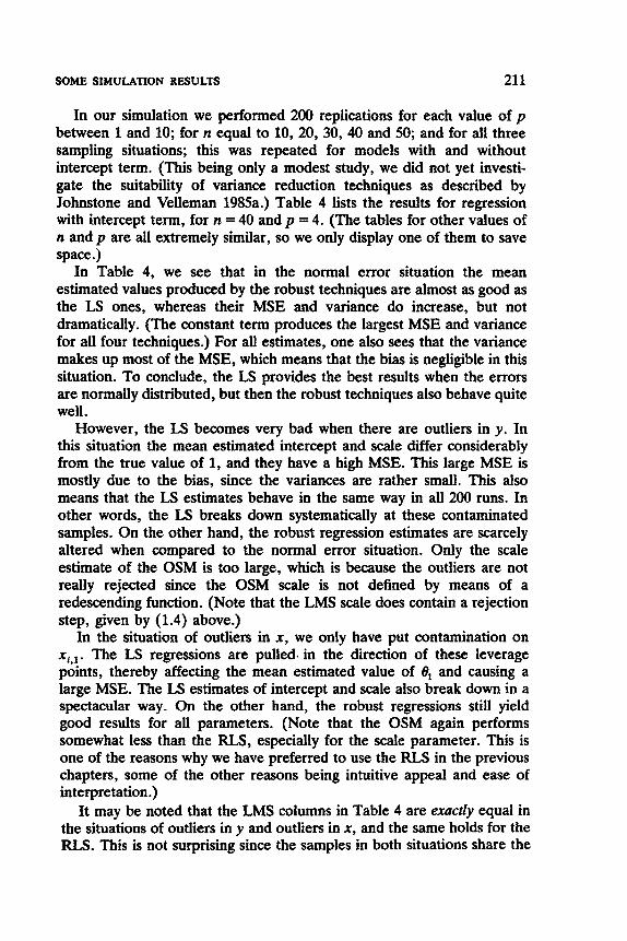
SOME SIMULATION RESULTS 21 1
In our simulation we performed 200 replications for each value of p between 1 and 10; for n equal to 10, 20,30, 40 and 50; and for all three sampling situations; this was repeated for models with and without intercept term. (This being only a modest study, we did not yet investi- gate the suitability of variance reduction techniques as described by Johnstone and Velleman 1985a.) Table 4 lists the results for regression with intercept term, for n = 40 and p = 4. (The tables for other values of n and p are all extremely similar, so we only display one of them to save space .)
In Table 4, we see that in the normal error situation the mean estimated values produced by the robust techniques are almost as good as the LS ones, whereas their MSE and variance do increase, but not dramatically. (The constant term produces the largest MSE and variance for all four techniques.) For all estimates, one also sees that the variance makes up most of the MSE, which means that the bias is negligible in this situation. To conclude, the LS provides the best results when the errors are normally distributed, but then the robust techniques also behave quite well.
However, the LS becomes very bad when there are outliers in y. In this situation the mean estimated intercept and scale differ considerably from the true value of 1, and they have a high MSE. This large MSE is mostly due to the bias, since the variances are rather small. This also means that the LS estimates behave in the same way in all 200 runs. In other words, the LS breaks down systematically at these contaminated samples. On the other hand, the robust regression estimates are scarcely altered when compared to the normal error situation. Only the scale estimate of the OSM is too large, which is because the outliers are not really rejected since the OSM scale is not defined by means of a redescending function. (Note that the LMS scale does contain a rejection step, given by (1.4) above.)
In the situation of outliers in x , we only have put contamination on xi,,. The LS regressions are pulled. in the direction of these leverage points, thereby affecting the mean estimated value of 0, and causing a large MSE. The LS estimates of intercept and scale also break down in a spectacular way. On the other hand, the robust regressions still yield good results for all parameters. (Note that the OSM again performs somewhat less than the RLS, especially for the scale parameter. This is one of the reasons why we have preferred to use the RLS in the previous chapters, some of the other reasons being intuitive appeal and ease of interpretation.)
It may be noted that the LMS columns in Table 4 are exactly equal in the situations of outliers in y and outliers in x , and the same holds for the RLS. This is not surprising since the samples in both situations share the

Tab
le 4
. Si
mul
atio
n R
esul
ts o
f R
egre
ssio
n w
ith I
nter
cept
, fo
r n
= 40 a
nd p
= 4
(Inc
ludi
ng th
e C
onst
ant T
erm
)"
Nor
mal
O
utlie
rs in
y
Out
liers
in x
Para
met
er
LS
LM
S RLS
OSM
Ls
LMS
RLS
OSM
LS
LMS
RLS
OSM
4 1.
0003
65
1.00
1555
l.O
007%
1.
0008
29
0.99
9226
0.
9996
41
0.99
9238
0.
9993
67
0.04
2766
0.
9996
41
0.00
0279
0.
0013
50
0.00
0479
0.
0006
19
0.00
4935
0.
0012
62
0.00
0430
0.
0005
56
0.91
8092
0.
0012
62
0.00
0279
0.
0013
47
0.00
0479
0.
0006
18
0.00
4934
0.
0012
62
0.00
0429
0.
0005
56
0.00
1794
0.
0012
62
1.oo
o884
1.
0(32
744
1.00
1689
1.
0021
17
1.00
4542
1.
0033
53
1.00
12uI
1.
0029
02
1.00
6389
1.
0033
53
O.oo
o268
0.
0013
20
O.o
oo48
1 0.
0005
70
0.00
4563
0.
0016
46
0.00
0533
0.
0007
26
0.02
2725
0.
0016
46
0.00
0267
0.
0013
13
0.00
0478
0.
0005
65
0.00
4542
0.
0016
35
0.00
0532
0.
0007
17
0.02
2684
0.
0016
35
4 0.
9991
25
0.99
6997
0.
998o
Oo
0.99
7707
0.
9975
24
0.99
7381
0.
9975
42
0.99
7274
0.
9873
13
0.99
7381
0.
0003
01
0.00
1598
O
.ooo
625
O.o
oo78
5 0.
0050
07
0.00
1500
0.
0004
92
O.OOO694
0.03
1526
0.
0015
00
0.00
0Mo
0.00
1589
O
.ooo6
21
O.ooo780
0.00
5001
0.
0014
93
O.OOO486
0.00
0687
0.
0313
65
0.00
1493
Con
stan
t 0.
9998
92
1.00
7599
0.
9899
71
0.99
0862
2.
9948
85
0.98
1571
1.
0049
95
0.99
6266
0.
2920
98
0.98
1571
0.
0234
51
0.12
7050
0.
0340
34
0.04
0130
4.
0410
06
0.10
9773
0.
0339
47
0.04
5180
3.
0897
55
0.10
9773
0.
0234
51
0.12
6992
0.
0339
34
0.o4
0046
0.
0614
41
0.10
9434
0.
0339
22
0.04
5166
2.
5886
30
0.10
9434
0
0.99
3785
0.
9375
18
0.86
1388
1.
0298
84
4.15
6255
1.
0945
57
0.93
7264
1.
4424
10
9.68
0913
1.
0945
57
0.01
3573
0.
0435
11
0.04
7492
0.
0384
12
10.0
0501
9 0.
0479
54
0.02
6198
0.
2588
37
76.7
4552
9 0.
0479
54
0.01
3535
0.
0396
07
0.02
8219
0.
0375
19
0.04
3075
0.
0390
12
0.02
2262
0.
0631
10
1.38
7274
0.
0390
12
6
'The
ent
ries
in e
ach
cell
are
the
mea
n es
timat
ed v
alue
, the
mea
n sq
uare
d er
ror,
and
the
var
ianc
e ov
er t
he 2
00 r
uns.
0.99
9238
0.
0004
30
0.00
0429
1.00
1238
0.
0005
33
0.00
0532
0.99
7542
O.ooo492
0.O
0048
6
1.00
4995
0.
0339
47
0.03
3922
0.93
7264
0.
0261
98
0.02
2262
0.99
9365
0.
0012
24
0.00
1223
1 .am95
0.oM
mo
O.o
oo7u
0.99
6846
o.
ooo7
31
0.oQ
oTz1
0.99
7807
0
.m
1
0.01
0867
1.46
1946
0.
2801
85
O.W
KM
l
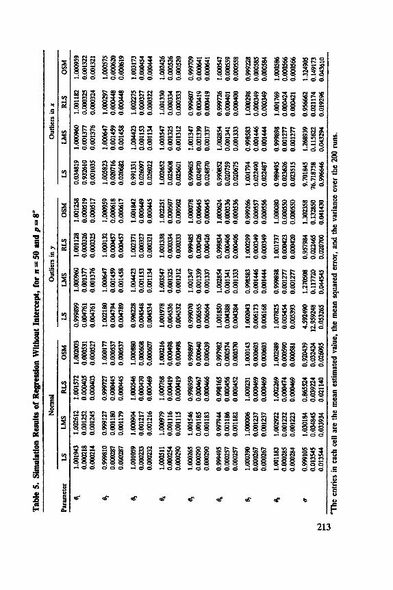
ELI69I'O
S06VzE'I
99WO
99sooo'o 98WI
Wooo'O
s8sooo'o 822666'0
8SS
00'0 6
SW
O
Lpmoo'l
Itr9oOo'O
199ooo'o 6oL666'0
ozsooo'o 9zsooo'o 9Z
puK)'I
PPP000'0 pspooo'0 E
LIE00'I
619000'0 oz9ooo'o S
LSooo'I
IZEIOO
'O
UE
I00'0 6S6000' I
9LIIu)'O
-0
IZ
WO
VzM
N0-0
69LIW
I
6HW
O'O
6pEoO
o'O
862000' I
00P000'0
Iowoo'0
9ZL666'0
61
WO
6
1W
'O
L4XJ666.0
CEEooo'O PEEooo'O
oEEI00'I
ZZEooo'O LZEooo'O
SLZM
O'I
8pw
oo
'O
W0
L6UlO
O.1
9ZEooo'O
SZ
EW
O
281100'1
U9S
II'O
6E68921
uz100'0 U
ZI00'0
868666'0
~1
00
'0
9Ptr100'0 €84366.0
ECE100'0 ItE
100'0 PSBMO'I
LEE100'0 6EE100'0 LV
CI00'I
ZIC100'0
SZEI00'0 L9SE00'1
9E1100'0
CSI100'0
€Z
M'I
8S9100'0
6S9100'0
Lp9ooO.1
9LEIW
O
UE
100'0 096000.1
8SL81C9L
SH
IOC
6
SISEM'O 9
ZW
O
S6
W6
0
L8m4S
O
069220'0 V6L100' I
SL
WO
6S
UTu)'O
zs8066.0
oL89zo'o OLBPZO'O so9666.0
109su)'o 809E
U)'O
Zs97KNJ.I
zmm
o L609U)'O IC
C166'0
z89oU)'o
91LOZWO
EEBW
I
SEOI00'0
019ZWO
618K
OO
OS8z€I~O 8SEM
E' I
ossooo'o ossooo'o 080000'1
9S
SW
0
LSSooo'O
992666'0
9CSooo'O
9Esooo'o X
9000'I
s09000'0 sp
9o
oo
'o
8u)oOo'I
u)sooo'o uK
oo0'0 152200'1
spbooo'o 6-0 zp8100'1
LIwo0.0
819000'0 6S6000' I
LI
WO
61Sooo'O
8SZ100'1
s9blu)'o W
6LS60
OZ
W0
€
ZW
O
Lu.100'1
6t6ooo'O
6K000.0
662oo0'1
90P000'0
9owoo'O
pE8666-0
9Z
WO
9
ZW
O
W666.0
EE
UW
X)'O
PECooo'O 8EE100'1
IZEooo'O
LZEOOO'O ILE
MO
'I
LSpoOo'O
L
SW
O
Z€IOOo'I SZEZEOO'O R
EW
0
8z1100'1
OZLLII'O
80M
)LZI
uz100'0 u
z100'0 868666'0
w100'0
w100'0 €8WO
EEE100'0 IK
100'0 DSBM
O' I
LEE
IWO
6EE100'0 Lpc100'1
ZIC100'0
SZE
100'0 LPSEO
O'I
pcI100'0 ES1100'0 €Zpwo'I
8S9100'0 6S
9100'0 Lp9ooo'I
9LEI00'0
UE
I00'0 096000'1
WZbS
6Z1 06VZ62'9
E6ESWO
PSK
00'0 SZ8KlO
.1
891900'0 EL1900'0 EW
7BO.I
p8
EW
O
88
CW
O
058100'1
P9E
900'0 S
9W
O
ofR666.0
ZE
SW
O
9ES
WO
8L6100'1
VtS
WO
m
W0
8ZZ9E6.0
68
LW
O
116LWO
081200'1
19
LW
O
19
LW
O
668666'0
VzpzEOO
6E
poz6'0
18Sooo'O
06sooo'o 686200'1
-0 E09000'0 E
9Iooo'I
OLSooo'O
9LS
WO
E
BW
O
6SJOW
O
OP9000'0
M8866.0
86
WO
8
6W
O
91u)oo'I
u)9ooo'O 809000'0 088M
O.1
LESooo'O
LESooo'O
UIooo'I
LZSooo'O
ICSooo'O
Eo0U
w)'I
trzz6Eo'O tzzS98'0
69bOOO.O 9
LW
O
69zu
)o'I
69booo'O
69pooo'O
IEzooo'I
ZEpoO
o'O
9S
WO
s91866.0
99woo'O
L9troO
o'O
656866'0
61
WO
6
1W
O
69WOO.O
OL
~O
w
sm
1
sm
0
sm
0
-0
tOP000'0
sowoo'o
zLs100'1
mu)oo'I
S~
O'
O
p81oEOI
€ZZ100'0 Z€ZIO
o'O
zz
6m
I
LEZIOO
'O
LEZ100'0 900000'1
Z81100'0 981100'0 W
WO
€81100'0 s81100'0 9Ps100'1
511100'0 911100'0 6L6o00'1
91ZI00'0 LIZ100'0 W
lWJO
.1
6L1100'0 081100'0 LZ1666-0
S9ZI00'0
ZSZI00'0
Z19MO
'I
SVSEIOO
SOI666'0
t8ZlXUl.O s82ooo'o €81100'1
L9Moo'O
L9zoO
o'O
06Eooo'I
LSzJm
.0 LsuW
)o'O
S6
MO
06uw)o'O
06uw
)o'O
S9ZOOO.1
06u)o'O
9SzJm.O
IIsm
I
zumso
ECU
)OO
'O
6SO
IWI
LBUMO'O
-0 018666'0
V1u)oo'O 81uw
)o'O
€116100'1
214 ALGORITHMS
80% of “good” observations, whereas the 20% of outliers are properly rejected by the LMS and the lUS . This is no longer true for the OSM, because there the outliers still have an (albeit very small) influence.
Table 5 contains the summary statistics for regression without inter- cept, with n = 50 and p = 8. (The results for other choices of n and p are very similar and hence are not listed here,.) For the normal situation we arrive-at the same conclusions as before, the robust techniques behaving almost as well as LS.
In the presence of outliers in the response variable, we find that the LS coefficients are still quite good. This is because the model now forces the fit to go through the origin, so the contamination (as in Figure 4b) cannot move up the fit as in a model with intercept. (Moreover, the contamina- tion happens to be balanced about the origin, so the solution does not even tilt in this experiment.) However, the LS scale estimate clearly breaks down because all points are taken into account, including the bad ones. On the other hand, the robust estimators provide decent estimates of both the 4 and (r. The simulation results also show that the RLS is really an improvement on the LMS as the mean squared errors are decreased even more, particularly that of the scale estimate. This is not true for the OSM, which again overestimates cr because it does not really reject the outliers.
which cause the LS estimate of 0, to break down. As was to be expected, also the corresponding scale estimate explodes. Fortunately, the robust techniques yield satisfactory estimates for all quantities. Moreover, the RLS again constitutes a slight improvement on the LMS results.
The overall conclusion of these simulations is that the LMS indeed achieves the goals for which it was constructed, because it gives reason- able results in the normal situation and is also able to withstand substan- tial amounts of outliers in x and in y.
The last columns of Table 5 deal with the outliers in
EXERCISES AND PROBLEMS
Section 1
1. Illustrate that the LMS algorithm in PROGRESS is regression, scale, and affine equivariant by running one or more example@) in which you transform the data as in (4.2), (4.3), and (4.4) of Section 4 in Chapter 3.
2. Derive the probability (1.2).

EXERCISES AND PROBLEMS 215
3. Write down formulas expressing the regression coefficients 4 in terms of the regression results on the standardized data. Why are these formulas the same for LS, LMS, and RLS regression?
seetion 2
4. Why is it useful to look at more than one local minimum of the objective function (2.2)? Consider both computational and data- analytic aspects.
5. (Research problem) Is it true that one can do no better than O(n”) algorithms for computing affine equivariant high-breakdown regres- sion estimators?
Section 3
6. In Section 3 the computation times of the LMS, the LTS, and S-estimators are discussed. What do you think would be the total cost of a combination of LMS with a subsequent one-step improvement (either a one-step RLS or a one-step M-estimator)? Indicate the computation time of such an estimator in Figure 3.
Section 4
7. (Research problem) Why does the behavior of (4.1) depend on n and p being even or odd?

C H A P T E R 6
Outlier Diagnostics
1. INTRODUCTION
Outlier diagnostics are statistics that focus attention on observations having a large influence on the least squares (LS) estimator, which is known to be nonrobust. Several diagnostic measures have been designed to detect individual cases or groups of cases that may differ from the bulk of the data. The field of diagnostics consists of a combination of numeri- cal and graphical tools.
Many diagnostics are based on the residuals resulting from Ls. How- ever, this starting point may lead to useless results because of the following reason. By definition, LS tries to avoid large residuals. Con- sequently, one outlying case may cause a poor fit for the majority of the data because the LS estimator tries to accommodate this case at the expense of the remaining observations. Therefore, an outlier may have a small LS residual, especially when it is a leverage point (see Figure 2 in Section 1 of Chapter 1). As a consequence, diagnostics based on LS residuals often fail to reveal such points.
Another class of diagnostics is based 2n the principle of deleting one case at a time. For example, denote by O ( i ) the estimate of 8 computed from the sample without the ith case. Then the difference between 6 and @(i) gives the extent to which the presence of the ith case affects the regression coefficients. These are so-called single-case diagnostics, which are computed for each case i. It is possible to generalize this to multiple- case diagnostics for highlighting the simultaneous influence of several cases. Indeed, the deletion of one or more cases seems to be a logical way to examine their impact. However, it is not obvious at all which subset of cases should be deleted. It may happen that some points are jointly influential but the individual points are not! Moreover, the computations
216
Robust Regression and Outlier Detection Peter J. Rousseeuw, Annick M. Leroy
Copyright 0 1987 John Wiley & Sons, Inc. ISBN: 0-471-85233-3

THE HAT MATRIX AND LS RESIDUALS 217
involved are often infeasible because of the large number of subsets that would have to be considered.
Some quantities that occur frequently in classical diagnostics are the diagonal elements of the LS projection matrix H. This matrix is well known under the name of hat marrix, because it puts a hat on the column vector y = ( y,, . . . , y,,)'. This means that f = Hy, where f is the LS prediction for y. In fact, the diagonal elements of the hat matrix are often used as diagnostic tools in their own right. Section 2 is devoted to the hat matrix, because this matrix is a fundamental component of the classical diagnostics treated in Sections 3-5. We will discuss the advantages and disadvantages of these tools, which appear in statistical packages such as SPSS, BMDP, SAS, and others. In Section 6, we propose alternative diagnostics that avoid some shortcomings of the classical ones.
2. THE HAT MATRIX AND LS RESIDUALS
Consider the following situation. Each individual i = 1, . . . , n is observed on p + 1 variables (that is, p explanatory variables and one response variable). The n-by-1 vector of responses is denoted by y = ( y, , . . . , y,,)'. The linear model states that
y=XB+e, (2.1)
where X is the n-by-p matrix
x11 x12 . * .
X = (2.2)
8 is the vector of unknown parameten, and e is the error vector, that is, e = (e,, . . . ,
The hat matrix H mentioned above is defined by
H = X(X'X)-'X' . (2.3)
(We assume that X'X is invertible.) The n-by-n matrix H is called the hat matrix because it transforms the observed vector y into its LS estimate f=€Iy. It can easily be verified that H is idempotent (HH=H) and symmetric (H' = H). From (2.3), it follows that

218 OUTLIER DIAGNOSTICS
traceH=p (i.e., hi, =p) 1 = 1
(2.4)
because trace H = trace [X'X(X'X)-'1 = trace I, = p, where I, is the p-by- p identity matrix. Moreover, the rank of H also equals p. The fact that H is idempotent and symmetric implies that
hi, = (HH),, = C hijhji = C. h,h, , j - 1 j-1
hence
Furthermore, H is invariant under nonsingular linear transformations of the explanatory variables. Indeed, let A be a p-by-p matrix of full rank. If the explanatory variables are transformed as
H=XA, (2.6)
it easily follows that
In particular, it is possible to multiply all variables xi by a constant aj, corresponding to multiplication by the matrix
without affecting H. This is applied in the program PROGRESS in the case of regression through the origin (regression without a constant term), because there each explanatory variable xi is standardized by dividing it by a robust measure of its spread.
In the case of regression with a constant term, the same matrix algebra can be used by means of an artificial explanatory variable x, which is identical to 1. This means that

THE HAT MATRIX AND IS RESIDUALS 219
and H is again defined by (2.3) with this X. Then one can even transform the p - 1 “real” explanatory variables by
xi -+ ujxj + bj
without affecting H, because this amounts to applying (2.6) and (2.7) with the matrix
a, 0 - . * 0 0
0 0 ..- =p-1
0 0 A = (2.10)
b, b2 ..- bP-,
Therefore, the standardization performed in the program PROGRESS (subtracting the median of the xi and dividing by their spread) does not change H. As a consequence, it was rather easy to compute H in PROGRESS. In order to obtain H in the output, one has to answer YES to the question
DO YOU WANT TO COMPUTE OUTLIER DIAGNOSTICS? PLEASE ANSWER YES OR NO:
in the interactive input.
and r=y-fs ince The hat matrix also plays a central role in the covariance matrices of 9
cov(9) = (r2H
cov(r) = a2(I - H) , (2.11)
(2.12)
where r = ( r , , . . . , r,)‘ is the n-by-1 vector of Ls residuals. An intuitive geometric argument reveals a link between the diagonal
elements of H and the location of the points in the space of the explanatory variables. The set of p-dimensional points x (not necessarily observations) that satisfy
h, = x(X‘X)-’x‘ 5 m s hii (2.13)

220 OUTLIER DIAGNOSTICS
determine an ellipsoid (see, e.g., Montgomery and Peck 1982, p. 143). This ellipsoid contains the smallest convex set enclosing the n observa- tions. Consequently, one can say that the point x lies close to the bulk of the space formed by the explanatory variables if h, is small.
The above properties of H are helpful in understanding and interpret- ing its elements h,. From 9 = Hy it follows that the element h, of H has a direct interpretation as the effect exerted by the jth observation on j,.. Especially the diagonal elements hii are of interest, because they equal dy^,/dy,. Therefore, they measure the effect of the ith observation on its own prediction. A diagonal element hii of zero indicates a point with no influence on the fit. From (2.4) it is immediately clear that the avera e
&om which it follows that 0 5 hi, I 1 for all i . These limits are useful for interpreting the size of the effect on the prediction but do not yet tell us when h, is “large.” Most authors (Hoaglin and Welsch 1978, Henderson and Velleman 1981, Cook and Weisberg 1982, Hocking 1983, Paul 1983, Stevens 1984) determine potentially influential points by looking at the h, and paying particular attention to points for which hi,>2pln (some people also use the cut-off value 3pln) .
From (2.5), it follows that hi, = 0 implies h, = 0 for all j, and hii = 1 implies h , = 0 for all i except j. Both extremes can be interpreted in a data analytic way. A simple example of hii = 0 is provided by a point with all explanatory variables equal to zero in a regression model without intercept. The prediction 9, is then fixed at zero and is not affected by y , or by any other y j . O n the other hand, when h, = 1 we have f i equal to y i and consequently ri = 0. In other words, when hii = 1, the ith observation is fitted exactly by the regression hyperplane. When hii is large, that is, near 1, then (2.12) implies that the variance of the ith residual is almost zero. The main cause for this may be that the case in question has an unusually large influence on the LS regression coefficients. However, although the Ls residual is near zero, one cannot identify that case as a bad or a good point.
Let us now investigate the diagnostic power of the hii on some examples. In Table 1, the diagonal elements of the hat matrix are printed for the Hertzsprung-Russell diagram data (see Table 3 of Chapter 2). From the LMS regression, we know that the outliers (the giant stars) correspond to the indices 11, 20, 30, and 34. In Table 1, the hi, for these observations are larger than the cut-off value 2pln (0.085 in this case). Indeed, these stars are the most outlying in x-space.
From the scatterplot of the telephone data (Figure 3 of Chapter 2), it was clear that the responses associated with the years 1964-1969 were contaminated. However, the diagonal elements of the hat matrix (shown
value of the h,, is p ln . Moreover, (2.5) implies that hi, = hi + Cj,,i h,, f

Table 1. Diagonal Elements of the Hat Matrix, Squared Mabplanobis Distance, and Standardized, Studentized, and Jaddurifed LS Residuals for the Hertzspnrag-RusseU Diagram Data” Index h,, MD: ?,IS ti r ( i )
i ( O - O w (3.84) (2.50) (2.50) (2.50) 1 2 3 4 5 6 7 8 9 10 11 12 13 14 15 16 17 18 19 20 21 22 23 24 25 26 27 28 29 30 31 32 33 34 35 36 37 38 39 40 41 42 43 44 45 46 47
0.022 0.037 0.022 0.037 0.021 0.027 0.078 0.038 0.022 0.022 0.195 0.025 0.U29 0.044 0.021 0.024 0.023 0.024 0.023 w 0.021 0.021 0.024 0.030 0.023 0.024 0.021 0.023 0.023 w 0.023 0.037 0.026 u 0.023 0.046 0.034 0.026 0.034 0.025 0.023 0.026 0.031 0.026 0.036 0.026 0.024
0.043 0.738 0.027 0.738 0.001 0.271 2.592 0.783 0.027 0.043 2294 0.171 0.342 1.055 0.005 0.144 0.084 0.144 0.084 u.24 0.005 0.005 0.144 0.383 0.059 0.144 0.005 0.059 0.094 8.031 0.059 0.738 0.232 32.94 0.084 1.134 0.572 0.232 0.572 0.171 0.059 0.232 0.427 0.232 0.681 0.232 0.144
0.44 1.47
-0.18 1.47 0.30 0.90 -0.99 0.64 0.95 0.24 0.67 0.87 0.85 -1.92 -1.35 -0.69 -1.96 -1.40 -1.53 0.95 -1.13 -1.42 -0.97 -0.16 0.06
-0.54 -0.64 -0.15 -1.16 1.24
-1.00 0.34 0.47 1.66
-1.25 1.30 0.32 0.47 0.46 1 .a
-0.64 0.19 0.72 0.68 1.11 0.04
-0.83
0.44 1.50
-0.19 1.50 0.31 0.91
-1.03 0.65 0.96 0.25 0.75 0.88 0.86 -1.96 -1.36 -0.70 -1.98 -1.41 -1.55 1.06
-1.15 -1.43 -0.98 -0.16 0.07
-0.55 -0.65 -0.15 -1.17 1.38
- 1.01 0.34 0.48 1.85
-1.26 1.33 0.32 0.48 0.47 1.10
-0.65 0.19 0.73 0.69 1.13 0.05 -0.84
0.44 1.52
-0.18 1.52 0.31 0.91 -1.03 0.64 0.96 0.24 0.74 0.88 0.86 -2.03 -1.38 -0.69 -2.05 -1.43 -1.58 1.06
-1.15 -1.45 -0.98 -0.16 0.07 -0.55 -0.64 -0.15 -1.18 1.40
-1.01 0.34 0.47 1.91
-1.27 1.35 0.32 0.47 0.46 1.10
-0.65 0.19 0.73 0.69 1.13 0.05 -0.84
‘The c u t 4 value for h,, is 2pln =O0.8S, and that for MD: is x:.~.,, = 3.84. 221

222 OUTLIER DIAGNOSTICS
in Table 2) do not point to outlying observations. This example illustrates that outliers in the y-direction are totally neglected by the hat matrix, because H is only based on the x i . Further on, we will discuss classical diagnostics that were designed especially to detect such outlying observa- tions.
An unfortunate property of the hii diagnostics is their vulnerability to the masking effect. To show this, let us consider the data set generated by Hawkins, Bradu, and Kass (1984), which was reproduced in Table 9 of Chapter 3. Since the cut-off value for the hii is 0.107, we would conclude from Table 3 that the cases with indices 12, 13, and 14 are suspect. However, from the construction of the data it is known that only the first
Table 2. Diagonal Ekments of the Hat Matrix, Quared Mahalambis Distance, and Standardized, Studentized, and Jackknifed LS Residuals for the Telephone Data" Index Year hi, MD;
i X; (0.167) (3.84) r,ls 4 (2.50) (2.50)
r(i) (2.50)
1 2 3 4 5 6 7 8 9 10 11 12 13 14 15 16 17 18 19 20 21 22 23 24
50 51 52 53 54 55 56 57 58 59 60 61 62 63 64 65 66 67 68 69 70 71 72 73
0.157 0.138 0.120 0.105 0.w1 0.078 0.068 0.059 0.052 0.047 0.044 0.042 0.042 0.044 0.047 0.052 0.059 0.068 0.078 0.091 0.105 0.120 0.138 0.157
2.653 2.216 1.802 1.457 1.135 0.836 0.606 0.399 0.238 0.123 0.054 0.008 0.008 0.054 0.123 0.238 0.399 0.606 0.836 1.135 1.457 1.802 2.216 2.653
~~
0.22 0.24 0.14 0.15 0.05 0.05
-0.02 -0.02 -0.10 -0.10 -0.18 -0.18 -0.25 -0.26 -0.33 -0.34 -0.39 -0.40 -0.45 -0.46 -0.51 -0.53 -0.58 -0.59 -0.65 -0.66 -0.65 -0.66 1.00 1.03 1.00 1.03 1.23 1.27 1.45 1.50 1.77 1.84 2.21 2.32
-0.89 -0.94 -1.31 -1.40 -1.35 -1.45 -1.40 -1.53
0.24 0.14 0.05
-0.02 -0.10 -0.18 -0.26 -0.33 -0.39 -0.45 -0.52 -0.58 -0.65 -0.65 1.03 1.03 1.29 1.54 1.95 2.60
-0.93 - 1.43 -1.49 -1.58
The cut-off vaue for hii is 2pln = 0.167, and that for h4D: is &9s = 3.84.

THE HAT MATRIX AND LS RESIDUALS 223
Table 3. Diagonal Elements of the Hat Matrix, Squared Mahalanobis Distance, and Standardized, Studentized, and Jackknifed LS ResiduaIs for the Hawkins- BrPdU-Kass Data"
Index hii MD: rils ti t ( i ) i (0.107) (7.82) (2.50) (2.50) (2.50)
1 0.063 3.674 1 so 1.55 1.57 2 0.060 3.444 1.78 1.83 1.86 3 0.086 5.353 1.33 1.40 1.41 4 0.081 4.971 1.14 1.19 1.19 5 0.073 4.411 1.36 1.41 1.42 6 0.076 4.606 1.53 1.59 1.61 7 0.068 4.042 2.01 2.08 2.13 8 0.063 3.684 1.71 1.76 1.79 9 0.080 4.934 1.20 1.26 1.26
10 0.087 5.445 1.35 1.41 1.42 11 0.094 5.986 - -3.48 -3.66 - -4.03 12 0.144 - 9.662 - -4.16 -4.50 - -5.29
14 - 0.564 40.725 -1.69 - -2.56 -2.67
Only the first 14 cases are listed. The cut-off value for h, is 0.107, and that for MD: is
13 - 0.109 7.088 -2.72 -2.88 - -3.04
x:.0.95 = 7.82.
10 observations are leverage outliers, whereas the next four cases (11,12, 13, and 14) are good leverage points. Therefore, the real outliers are masked by the effect of good leverage points. As far as the hat matrix is concerned, some leverage points may be masked by others.
In the case of regression with a constant, one also measures leverage by means of the MuhuZunobis distance. Let us first split up the x i into the essential part vi and the last coordinate 1:
x i = (xi,l * * * q p - l 1) = (Vi 1) ,
where
vi = ( X i J - * * q p - l )
is a ( p - 1)-dimensional row vector. One computes the arithmetic mean ? and the covariance matrix C of these vi:
1 " n i = l
T = - &

224 OUTLIER DIAGNOSTICS
1 " n - 1 i - 1
C=- 2 (Vi - T)'(Vi - V) .
One then measures how far vi is from T in the metric defined by C, yielding
MD: = (vi - s)c-'(v, - t)' , (2.14)
which is called the s uared Mahalanobis distance of the ith case. The purpose of these MD, is to point to observations for which the explana- tory part lies far from that of the bulk of the data. For this reason, several packages (notably BMDmR, SAS, and SPSS) compute the squared Mahalanobis distance. The values of MD; may be compared with quan- tiles of the chi-squared distribution with p - 1 degrees of freedom (in Tables 1-3, the MD: are compared with the 95% quantiles).
It turns out that there is a one-to-one relationship between the squared Mahalanobis distance and the diagonal elements of the hat matrix, given
9
bY
MD; = (n - 1)[ hii - ;] , (2.15)
which provides another clarification of the meaning of the hii. To prove (2.15), we first note that we may subtract the average of each of the first p - 1 explanatory variables, because this changes neither the hat matrix nor the MD:. Therefore, we may assume without loss of generality that ( l ln) E:,,l xij = 0 for each variable j = 1,. . . , p - 1, hence S = 0. Therefore,

THE HAT MATRIX AND LS RESIDUALS 225
from which it follows that
hi, = xi(x‘x)-’x;
1 n - 1 n M D ~ + - ,
1 =-
which proves (2.15). The hat matrix is useful when the data set contains only a single
observation with outlying xi. However, when there are several such observations, it may easily happen that this does not show up in the corresponding hii. The reason for this is that (2.14) is based on a classical covariance matrix, which is not robust. Therefore, there may be multiple outliers in x which do not show up through the hat matrix. To conclude, we think that it is not appropriate to define “leverage” in terms of h,. Rather, one should say that leverage points are any outliers in x-space (which may be more difficult to identify), because such points have a potentially large influence on the fit. In order to discover such leverage points, it is better to insert a robust covariance estimator in (2.14). More details on this can be found in Section 1 of Chapter 7 (two examples on the identification of leverage points are given in Subsection Id of Chapter 7).
At any rate, examining the hii alone does not suffice when attempting to discover outliers in regression analysis, because they do not take yi into account. For a long time, one has thought that the LS residuals possess all the complementary information. We will restrict our attention to the standardized, the studentized, and the jackknifed residuals. The packages SPSS and SAS provide these statistics in their regression programs. However, these packages do not use a uniform terminology.
In the LS part of the PROGRESS output, we computed the standar- dized residuals defined as
where s2 is given by
(2.16)

226 OUTLIER DIAGNOSTICS
(2.17)
When the measurement errors on yi are independent and normally distributed with mean zero and standard deviation a, it is known that s2 is an unbiased estimator of a’.
Many authors (Cook 1977, Hoaglin and Welsch 1978, Draper and John 1981, Atkinson 1982, Cook and Weisberg 1982, Hocking 1983, Hocking and Pendleton 1983, Paul 1983, Stevens 1984) have taken (2.12) into account for the scaling of the residuals. They recommend the studentized residuals
(2.18)
In the literature these are sometimes called “standardized residuals”. Then, the term “studentized residual” is mostly applied to
r
(2.19)
where s(i) is the estimate of a when the entire regression is run again without the ith case. We will call the t(i) jackknifed residuals. Velleman and Welsch (1981) and Cook and Weisberg (1982) call f , an “internally studentized residual” and t(i) an “externally studentized residual”, whereas Belsley et al. (1980) used the term “RSTUDENT” for qi). Atkinson (1983) referred to (i) as “cross-validatory residual”.
We will now illustrate these diagnostics on the three examples for which we discussed the diagonal elements of the hat matrix earlier. Table 1 gives the squared Mahalanobis distance and the standardized, studen- tized, and jackknifed LS residuals for the Hertzsprung-Russell data. The squared Mahalanobis distance confirms the information that was already apparent from the hii. On the other hand, none of the residuals shows the presence of outliers, as they are all very small (much smaller than 2.5). This phenomenon is typical for data sets containing multiple outliers in the x-direction: neither the standardized residuals nor the transformed residuals detect the outliers because the latter have pulled the LS fit in their direction.
Let us now look at these residuals for the telephone data (Table 2), which is a sample containing outliers in the y-direction. Although at least six observations (the years 1964-1969) contained a wrongly recorded response variable, none of the residuals in Table 2 are really large. This is because s and s(i) explode in the presence of outliers.

SINGLE-CASE DIAGNOSTICS 227
The effectiveness of diagnostics becomes much more important in multiple regression models. Therefore, let us investigate the squared Mahalanobis distance and the standardized, studentized, and jackknifed residuals for the Hawkins-Bradu-Kass data set. Table 3 is restricted to the first 14 observations because these are the interesting ones (all the other cases yield small values anyway). Because of (2.15), the observa- tions with a high MDT also have a high h,. The three types of residuals are small everywhere, except for the observations 11, 12, and 13. Unfortunately, these observations should have small residuals because they were not generated as outliers. None of the table entries indicates the true outliers in this data set.
3. SINGLE-CASE DIAGNOSTICS
In order to assert the influence of the ith observation, it is useful to run the regression both with and without that observation. For this purpose, Cook's squared distance (Cook 1977) measures the change in the regres- sion coefficients that would occur if a case was omitted. It is defined by
(3 - s(i))'M(8 - &i)) C
CD2(i) = 9
where 6 is the LS estimate of 8, and i ( i ) is the LS estimate of 8 on the data set without case i. Usually, one chooses M = X'X and c = ps2. Alternative choices for M and c lead to other diagnostics. In words, CDZ(i) is the squared standardized distance over which 8 moves when estimated without the ith case. A large value of CD2(i) indicates that th_e ith observation has a considerable influence on the determination of 8, An approximate (1 - a ) x 100% confidence ellipsoid for 8 centered at 8 is given by the set of all 8* such that
(3.2) (e* - i)'(x'x)(e* - i)
P S Z
is less than the (1 - a)-quantile of an F-distribution with p and n - p Gegrees of freedom. So, the removal of the ith data point, which yields 8(i), would lead to the shift of the LS estimate to the edge of an (1 - a) x 100% confidence region based on the complete data. However, CD2(i) is not really distributed as an F-statistic. The F-distribution has merely been introduced by analogy to the theory of a confidence region for the LS estimate of 8 because it allows one to assess the magnitude of

228 OUTLIER DIAGNOSTICS
CD’(i). Most authors (Cook and Weisberg 1982, Montgomery and Peck 1982) indicate that a CD’(i) of about 1.0 would generally be considered large.
Making use of 9 = X6, Cook‘s squared distance can also be written as
This equivalent form allows us to say that CD’(i) measures the effect of deleting the ith observation on the fitted value vector. Another revealing form is
1 hi, CD’(i)= - t: - .
p 1- hii (3.4)
From this equation it follows immediately that CD2(i) depends on three relevant quantities, all of which are related to the full data set. These quantities are the number of coefficients the ith studentized residual, and the ratio of the variance of y, [i.e., u hiit see (2.11)] to the variance of the ith residual [i.e., ~‘(1- h,,), see (2.12)l. Thus CD2(i) is made up of a component that reflects how well the model fits y, and a component that measures how far xi is from the rest of the xi. Both may contribute to a large value of CD’(i). Formula (3.4) is very similar to one of the diagnostics of Belsley et al. (1980), namely
P
ri (hi,)“* DFFITS(i) = - - ~ ( i ) 1 - hii
(3.5)
(the only essential difference is the use of s(i) instead of s). In fact, DFFITS(i) originates from the standardization of the ith component of 4 - s(i), so this diagnostic measures the influence on the prediction when an observation is deleted. Observations for which D m T S exceeds 2(pln)”’ should be scrutinized. In an analogous way, Belsley et al. (1980) defined a diagnostic based on the change in the jth regression coefficient, namely
DFBETASj(i) = Cji T i
[C;,, c;~]”’ s(i)(l- hi,) ’
where C = (X’X)-’X‘ is sometimes called the catcher matrix. The cut-off value for DFBETAS is 2 / a . (Polasek 1984 treated an extension to general error structures for the residuals.) Belsley et al. also examine some other quantities in order to investigate whether the conclusions of hypothesis testing could be affected by the deletion of a cast. They

SINGLE-CASE DIAGNOSTICS 229
consider for example the t-statistic (for testing whether the jth regression coefficient is significantly different from zero) and compute
This diagnostic measures the difference between the t-statistic corres- ponding to the whole data set and that corresponding to the data set without case i.
It is worth noting that all these diagnostics are characterized by some function of the LS residuals, the diagonal elements of the hat matrix, and/or elements of the catcher matrix. These building blocks contain two types of information: the LS residuals ri are measures of poor fit, and the hat matrix and the catcher matrix reflect the remoteness of x i in the space of the explanatory variables. Unfortunately, their interpretation is no longer reliable when the data contains more than one outlying case. These diagnostics are susceptible to the masking effect, because two or several outliers can act together in complicated ways to reinforce or to cancel each other's influence. The final result is that these single-case diagnostics often do not succeed in identifying the outliers.
Most standard statistical packages provide single-case diagnostics. From SPSS one can obtain Cook's squared distance, and SAS also yields DFFITS and DFBETAS. Velleman and Welsch (1981) presented a survey of the field and clarified some conflicting terminology. They gave for- mulas for the efficient computation of regression diagnostics and men- tioned statistical programs from which some diagnostics can be obtained.
Let us now apply these single-case diagnostics to the data sets consi- dered above. Cook's squared distance, DFFITS, and DFBETAS appear in Tables 4-6 for the Hertzsprung-Russell data, the telephone data, and Hawkins' data set. The cut-off value for each diagnostic is printed in parentheses at the top of the corresponding column. Values exceeding this cut-off are underlined.
For these data sets, we are well aware of the position of the outliers. This makes it easy to evaluate the information provided by these single- case diagnostics. For the Hertzsprung-Russell data, we see that the outliers are not noticed by CD*(i). The DFFITS and DFBETAS diagnos- tics for the cases 14,20, 30, and 34 (also 11 for DFBETAS) are larger in absolute value than the cut-off value. Apart from 14, these cases were also considered as outlying by least median of squares (LMS) in Chapter 2.
The telephone data seem to be very tough for the single-case diagnos- tics. Cook's squared distance remains below the cut-off value 1.0

Table 4. Outlier Diagnostics (Including the Resistant Diagnostic RD,, which wil l be explained in Section 6) for the Hertzsprung- Russell Diagram Data“
RD, DFBETAS (0.292) Index CD*(i) DFFITS
i (1.Oo0) (0.413) Intercept Slope (2.500)
1 2 3 4 5 6 7 8 9
10 11 12 13 14 15 16 17 18 19 20 21 22 23 24 25 26 27 28 29 30 31 32 33 34 35 36 37 38 39 40 41 42 43 44 45 46 47
0.002 0.044 O.Oo0 0.044 0.001 0.012 0.044 0.008 0.010 0.001 0.068 0.010 0.011 0.089 0.020 0.006 0.046 0.025 0.028 0.137 0.014 0.022 0.012 O.Oo0 O.Oo0 0.004 0.005 O.Oo0 0.016 0.233 0.012 0.002 0.003 0.416 0.019 0.043 0.002 0.003 0.004 0.015 0.005 O.OO0 0.008 0.006 0.024 O.Oo0 0.009
0.066 0.300
-0.027 0.300 0.045 0.151
-0.298 0.128 0.144 0.037 0.366 0.141 0.147
-0.437
-0.109 -0.315 -0.226 -0.242
0 2 -0.170 -0.215 -0.155 -0.028
0.010 -0.087 -0.095 -0.023 -0.182 m
-0.154 0.067 0.078
-0.1% 0.295 0.059 0.078 0.086 0.176
-0.098 0.031 0.129 0.113 0.219 0.007
-0.132
-0.203
-0.009 -0.181 -0.006 -0.181
0.005 -0.061 -0.264 -0.079
0.033 -0.005 0.353
-0.046 -0.066 -0.334 -0.027
0.032 -0.109
0.067 -0.083
0.505 -0.023 -0.029
0.046 0.013
-0.002 0.026
-0.013 0.004
-0.065 m 0.026
-0.041 -0.029 - 0.905
-0.067 -0.202 -0.033 -0.029 -0.048 -0.057
0.017 -0.012 -0.064 -0.043 -0.129 -0.003
0.039
0.014 0.197 0.005 0.197
-0.002 0.071 0.254 0.086
-0.024 0.008
-0.345 0.054 0.075 0.315 0.014
-0.039 0.089
-0.081 0.068
-0.495 0.012 0.014
-0.056 -0.015
0.002 -0.031
0.006 -0.005
0.054 -0.651 -0.037
0.044 0.034
-0.886 0.055 0.216 0.036 0.034 0.052 0.068
-0.023 0.014 0.071 0.050 0.141 0.003
-0.047
0.841 1.111 1.194 1.111 1.189 0.772 rn 0.882 1.885 0.700 rn 0.833 0.769 2.290 1.422 0.m 1.819 1.421 1.553 7.163 1.289 1.467 1.154 0.845 0.599 0.888 0.979 0.650 1.320 - 7.364 1.182 1.000 0.585
1.376 1.108 0.806 0.585 0.725 0.978 0.960 0.516 0.734 0.682 0.947 0.522 1.066
The cutoff value for DFlRTS is 2( pln)”’ = 0.413, and for DFBETAS it is 2lVT = 0.292.
230

SINGLE-CASE DIAGNOSTICS 23 1
Table 5. Outlier Diagnostics (Including the Resistant Diagnostic RD,) for the Telephone Data
mi Index Year CD2(i) DFFITS DFBETAS (0.408)
i xi (1.OOO) (0.577) Intercept Slope (2.500)
1 50 2 51 3 52 4 53 5 54 6 55 7 56 8 57 9 58
10 59 11 60 12 61 13 62 14 63 15 64 16 65 17 66 18 67 19 68 20 69 21 70 22 71 23 72 24 73
0.005 0.002 O.OO0 O.OO0 0.001 0.001 0.002 0.004 0.004 0.005 0.006 0.008 0.010 0.010 0.026 0.029 0.051 0.082 0.144 0.267 0.051 0.134 0.169 0.217
0.101 0.057 0.018
-0.008 -0.032 -0.052 -0.069 -0.083 -0.092 -0.101 -0.111 -0.122 -0.137 -0.139
0.229 0.242 0.324 0.417 0.570 - 0.821
-0.319 -0.530 -0.597 -0.681
0.092 0.051 0.016
-0.007 -0.026 -0.040 -0.049 -0.053 -0.050 -0.045 -0.035 -0.022 -0.006
0.014 -0.053 -0.085 -0.145 -0.221 -0.341 -0.538
0.223 0.391 - 0.458 0.541
-0.087 -0.048 -0.014
0.006 0.024 0.036 0.043 0.046 0.041 0.034 0.023 0.009
-0.010 -0.030
0.078 0.109 0.177 0.259 0.390 - 0.604
-0.247 - -0.428 -0.498 - -0.584
1.054 0.946 0.835 0.731 0.624 0.518 0.472 0.439 0.490 0.584 0.677 0.772 0.867 1.566
34.566 35.879 41.632 47.042 54.502 64.352 - 6.251 1.754 1.835 1.924
everywhere. The contaminated years also go undiscovered by DFFITS and the DFBETAS. Worse still, these diagnostics point to "good" years as being outlying!
The Hawkins-Bradu-Kass data show that also multivariate outliers may be hard to find by means of single-case diagnostics (see Table 6). The cut-off value 1.0 for CD*(i) is only attained by observation 14, which is a good leverage point. Also DFFITS and DFBETAS do not succeed in separating the bad points from the good ones, whereas the LMS residuals did (see Section 3 of Chapter 3).
We will end this section with a discussion of some of the above diagnostics in connection with the data of Mickey et al. (1967) concerning the relation between age at first word and Gesell adaptive score. (We

232 OUTLIER DIAGNOSTICS
Table 6. Outlier Mpgnostics (Including the Resistant Diagnostic RD,) for the First 14 Cam of the Hawkins-Bradu-Kass Data
RD, DFBETAS (0.231) Index CD2(i) DFFITS
i (1,000) (0.462) Constant 8, 4 6, (2.500)
1 0.040 0.407 -0.076 0.116 -0.062 0.039 12.999 2 0.053 - 0.470 0.006 -0.043 0.006 0.092 13.500 3 0.046 0.430 -0.038 0.080 -0.180 0.160 13.911 4 0.031 0.352 0.045 -0.085 -0.070 0.161 13.961 5 0.039 0.399 -0.007 -0.001 -0.090 0.135 13.982 6 0.052 0.459 -0.141 0.201 -0.050 -0.019 13.451 7 0.079 0.575 -0.156 0.189 0.027 -0.055 13.910 8 0.052 - 0.464 -0.034 0.060 -0.108 0.121 13.383 9 0.034 0.372 0.055 -0.086 -0.103 0.191 13.718
10 0.048 0.439 0.098 -0.126 -0.167 0.273 13.535 11 0.348 -1.300 -0.052 0.238 0.174 -0.491 11.730 12 0.851 -2.1% -0.024 -0.025 1.192 -1.262 12.004 13 0.254 -1.065 0.367 -0.257 -0.424 0.359 12.297 14 2.114 -3.030 0.559 0.337 -2.795 1.920 13.674
already treated this example briefly in Chapter 2.) Many articles dealing with diagnostics use this data set as an illustration, but the conclusions are not unanimous. Mickey et al. (1967) themselves indicated observation 19 as an outlier. Andrews and Pregibon (1978) stated that case 18 is most influential and that 19 is not an outlier. On the other hand, Draper and John (1981) maintained that case 19 is an outlier, and they called case 18 an influential point. Dempster and Gasko-Green (1981) found that the pair of points 2 and 18 only extend the domain of the model and that case 19 was an outlier that does not matter. Paul (1983) summarized his analysis by saying that 18 is a high leverage point and that 19 is not an outlier. The hii , LS residuals, CD2(i), DFFITS, DFBETAS, and the weights based on LMS are reproduced in Table 7.
The weights determined by LMS regression are 1 everywhere except for case 19. The diagnostics that are designed to detect leverage focus their attention on observation 18, because it lies farthest away in the factor space (look at h, and CD2(i)). The standardized LS residual exceeds 2.5 (in absolute value) for observation 19 only. This is easy to understand. Since cases 2 and 18 are leverage points, they produce small LS residuals. Their joint position, isolated from the rest of the data, is the reason why the deletion of only one of them will not greatly affect the residuals. The singlecase diagnostic DFFITS points at observation 18
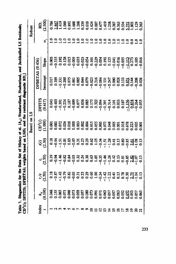
Tab
le 7
. D
iagn
ostic
s fo
r th
e D
ata
Set
of M
icke
y et
al.
[h,,;
Sta
ndar
dize
d, S
tude
ntiz
ed, a
nd J
ackk
nife
d L
S R
esid
uals
; C
D’(I
); D
FFIT
S; D
FBE
TA
S; w
eigh
ts b
ased
on
LMS;
and
the
res
ista
nt d
iagn
ostic
RD
,]
Bas
ed o
n LS
Rob
ust
DFBETAS
(0.4
36)
Inde
x h,
i ri
ls
ti
t(i)
C
D*(
i)
DFF
ITS
RD,
i (0
.190
) (2
.50)
(2
.50)
(2
.50)
(1.
OO
O)
(0.6
17)
Inte
rcep
t Sl
ope
wi
(2.5
00)
1 0.
048
2 0.
155
3 0.
063
4 0.
071
5 0.
048
6 0.
073
7 0.
058
8 0.
057
9 0.
080
10
0.07
3 11
0.
091
12
0.07
1 13
0.
063
14
0.05
7 15
0.
057
16
0.06
3 17
0.
052
18
0.65
2 19
0.
053
20
0.05
7 21
0.
063
0.18
0.
19
0.18
0.
001
-0.8
7 -0
.94
-0.9
4 0.
081
-1.4
2 -1
.46
-1.5
1 0.
072
-0.7
9 -0
.82
-0.8
1 0.
026
0.82
0.
84
0.83
0.
018
-0.0
3 -0
.03
-0.0
3 O.
OO0
0.31
0.
32
0.31
0.
003
0.23
0.
24
0.23
0.002
0.29
0.
30
0.29
0.
004
0.60
0.
63
0.62
0.
015
1 .oo
1.05
1.
05
0.05
5 -0
.34
-0.3
5 -0
.34
0.00
5 -1
.42
-1.4
6 -1
.51
0.07
2 -1
.22
-1.2
6 -1
.28
0.04
8 0.
41
0.42
0.
41
0.00
5 0.
13
0.13
0.
13
0.00
1 0.
78
0.81
0.
80
0.01
8 -0
.50
-0.8
5 -0
.85
0.67
8 2.7
5 &
@
3.61
0.22
3 -1
.04
-1.0
7 -1
.08
0.03
5 0.
13
0.13
0.
13
0.00
1
0.04
1 -0
.403
-0
.391
-0
.224
0.
187
-0.0
09
0.07
7 0.
056
0.08
5 0.
173
0.32
2 -0
.094
-0
.391
-0
.314
0.
101
0.03
3 0.
187
-1.1
56
0.854
-0.2
64
0.03
3
0.01
7 0.
189
-0.3
31
-0.2
00
0.07
5 0.
001
0.00
5 0.044
0.07
9 -0
.023
0.
316
-0.0
84
-0.3
31
-0.2
47
0.08
0 0.
028
0.13
3 0.
831
0.14
4 -0
.208
0.
028
0.00
3 -0
.335
0.
192
0.12
8 0.
015
-0.0
05
0.03
3 -0
.023
-0
.054
0.
101
-0.2
29
0.05
4 0.
192
0.12
5 -0
.041
-0
.016
-0
.055
-1
.113
0.
273
0.10
5 -0
.016
1.0
0.78
6 1.
0 2.8
67
1.0
1.41
9 1.
0 1.O
OO
1.0
0.89
2 1.
0 1.
688
1.0
1.28
8 1.
0 0.
339
1.0
0.61
8 1.
0 1.
624
1.0
0.88
7 1.
0 0.
677
1.0
1.41
9 1.
0 1.
258
1.0
0.38
7 1.
0 0.
363
1.0
0.53
4 1.
0 5.752
0.0
1.80
3 1.
0 1.
129
1.0
0.36
3

234 OUTLIER DIAGNOSTICS
and, to a ksser extent, at 19. DFBETAS is larger than the cut-off value for case 18 only. For this sample, it is hard to draw an overall conclusion from the different diagnostics. This is because of the lack of observations between the pair of leverage points (2 and 18) and the remaining data points.
The present variety of single-case diagnostics appears rather over- whelming. Moreover, the single-case diagnostics, although simple fr6m a computational point of view, often fail to reveal the impact of small groups of cases because the influence of one point could be masked by another.
4. MULTIPLECASE DIAGNOSTICS
Most of the single-case diagnostics of Section 3 can be extended in order to assess the changes caused by the deletion of more than one observation at the same time. These generalizations are called multiple-case diugnos- tics. Because of constraints of computation time, they are less popular than their single-case counterparts. The diagnostics described here are the most widely used.
Cook and Weisberg (1982) generalized formula (3.1) to measure the joint effect of deleting more than one case, yielding
(6 - d(Z))'M(6 - 6(Z)) C
CD2(Z) = 7
yhere I represents the indices corresponding to a subset of cases, and @(I) is the LS estimate of 8 calculated without the cases indexed by I. Again, several possibilities for M and c can be used, such as M = X'X and c = f . The quantity CD2(Z) can be interpreted in an analogous way as CD ( i ) . However, the selection of the cases to include in I is not obvious at all. It may happen that subsets of points are jointly influential but individual points are not. Therefore, single-case diagnostics do not indi- cate which subsets have to be considered. Moreover, the computation for all pairs, triples, and so on, leads to Cr runs, where m = 1, . . . , n/2. This is usually infeasible. This fundamental problem is shared by all diagnos- tics that require consideration of all subsets of cases.
Andrews and Pregibon (1978) proposed the determinantal ratio
det [Z'(Z)Z(Z)] AP(Z) =
det [Z'Z] '

RECENT DEVELOPMENTS 235
where Z is the X matrix with the response variable y appended, that is,
Z(Z) is the part of Z obtained by deleting the rows corresponding to the indices in Z, From (4.2) it is clear that AP(Z) is a dimensionless measure. Geometrically, one can interpret the quantity AP(Z) as a measure of the remoteness of the subset of cases with indices Z. This interpretation is based on the fact that 1 - AP(Z)1’2 corresponds to the relative change in the volume of an ellipsoid produced by Z’Z when the cases corresponding to the index set Z are omitted (Andrews and Pregibon 1978). Hence, it follows that small values of AP(Z) are associated with extreme cases, which may be influential. The conclusions drawn from Cook’s squared distance and the Andrews-Pregibon statistic are not necessarily similar. Little (1985) decomposes AP(Z) into two terms, which shows a relation between the AP statistic and Cook’s statistic. Both CD2(Z) and AP(I) are discussed in Draper and John (1981).
The extension of diagnostics to groups of cases appears to be conceptu- ally straightforward. However, they involve prohibitive computations if all possible subsets of cases are considered. Some strategies exist for approaching the computational problems, but none of them guarantees to identify all the bad cases present in the data set.
5. RECENT DEVELOPMENTS
Recently, Gray and Ling (1984) proposed to perform a k-clustering on the modified hat matrix
H* = Z(Z‘Z)-’Z‘ (5.1)
(where Z is again the X matrix with the y vector appended), in order to identify subsets of cases which are similar with regard to the elements of H*. In particular, they consider the elements of H* as similarity measures between the objects. Then they use the k-clustering algorithm in the hope of discovering a block-diagonal structure in H*. They perform the clustering for several values of the unknown parameter k. These cluster- ings yield (in a very ad hoc way) different candidate subsets that then have to be evaluated by one or more multiple-case diagnostics. The clustering results appear to be rather ambiguous, but in principle this

236 OUTLIER DIAGNOSTICS
approach avoids the treatment of all possible subsets of cases. However, the basic problem with the hat matrix remains: It breaks down easily in the presence of multiple outliers, after which it does not even contain the necessary information on the outliers anymore. Therefore, one cannot be sure that all bad subsets will be discovered.
Another step in the development of diagnostics is the use of the “elemental sets” that have been proposed by Hawkins et al. (1984). The underlying idea resembles the algorithm for the LMS. They also use random subsets J consisting of p observations. They call such a J an elemental set. The estimate determined by these p observations is called the “elemental regression” 0, and is equal to the “pseudo-observation” used by Oja and Niiminaa (see Section 6 of Chapter 3). Then they define the “elemental predicted residuals” ri(O,) resulting from the elemental regression 0, by means of
In order to summarize the information in all subsets, they look at the median of the elemental predicted residuals over all subsets J ,
” ri = med ri(6,) , J (5.3)
for each case i. An observation for which this statistic is large may be identified as outlying. Unfortunately, this technique does not have a very good breakdown point. Indeed, E* decreases fast with the dimension of the problem:
& * = l - ( q ) 1 1lP . (5.4)
This expression for the breakdown point is derived from the condition that the “good” subsets J have to be in the majority in order for the median in (5.3) to be meaningful. More formally, the probability of selecting a subset of p good points out of a sample that may contain a fraction E of contamination must be greater than 50%. This yields
(1 - E ) ~ r 5 0 % ,
which is equivalent to
giving the upper bound on the amount of contamination E that may be

HIGH-BREAKDOWN DIAGNOSTICS 237
tolerated. The same reasoning was already applied to the Theil-Sen estimator [formula (7.3) in Section 7 of Chapter 21 and its generalization due to Oja and Niinimaa [formula (6.6) in Section 6 of Chapter 31. Table 21 in Section 6 of Chapter 3 lists the resulting breakdown point for some values of p.
Hawkins et al. (1984) tested the elemental set method on their artificial data set (which we discussed in Sections 2 and 3 of this chapter). The proportion of outliers in this data set is close to the breakdown point of the elemental set technique. Hawkins et al. applied four iterative algorithms, one of w?lich uncovered the real outliers. On the other hand, we saw in Chapter 3 that the LMS easily finds them.
6. HIGH-BREAKDOWN DIAGNOSTICS
We need diagnostics that are able to cope with multiple outliers, without suffering from the masking effect. That is, we want diagnostics that have high breakdown. One way to formalize this objective would be to compute the breakdown point of the estimator defined by (a) deleting all observations for which the diagnostic exceeds its cutoff, and then (b) applying LS to the remainder. We shall look at two ways to construct such “sturdy” diagnostics.
a. Residuals from Robust Fits
As already indicated in Section 2, the residuals from an LS fit are not very useful as outlier diagnostics. On the other hand, the residuals computed from a very robust estimator embody powerful information for detecting all the outliers present in the data. In particular, one can look at the standardized LMS residuals r j h * (with CT* as defined in Chapters 2 and 5 ) , which are dimensionless. A plot of these standardized residuals versus the estimated value of y j or versus the index i gives a visual portrayal of this quantitative information. Whatever the dimension of the original data set, these plots enable the data analyst to detect the bad points in a simple display. These tools (provided by PROGRESS) have been used extensively for the analysis of various examples in Chapters 2 and 3.
REMARK. While this book was already in press, a paper by Atkinson (1986) appeared in which the LMS residuals are used for the same purpose. Atkinson applies the LMS to “unmask” the outliers (i.e., to identify them), after which he cames out a second stage by means of LS
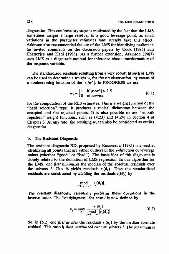
238 OUTLIER DIAGNOSTICS
diagnostics. This confirmatory stage is motivated by the fact that the LMS sometimes assigns a large residual to a good leverage point, as small variations in the parameter estimates may already have this effect. Atkinson also recommended the use of the LMS for identifying outliers in his invited comments on the discussion papers by Cook (1986) and Chatterjee and Hadi (1986). As a further extension, Atkinson (1987) uses LMS as a diagnostic method for inference about transformation of the response variable.
The standardized residuals resulting from a very robust fit such as LMS can be used to determine a weight wi for the ith observation, by means of a nonincreasing function of the lri/v*l. In PROGRESS we use
1 if Iri/a*ls2.5 0 otherwise
wi =
for the computation of the RLS estimates. This is a weight function of the “hard rejection” type. It produces a radical dichotomy between the accepted and the rejected points. It is also possible to use “smooth rejection” weight functions, such as (4.23) and (4.24) in Section 4 of Chapter 3. At any rate, the resulting wi can also be considered as outlier diagnostics.
b. The Resistant JHagnostic
The resistant diagnostic RD, proposed by Rousseeuw (1985) is aimed at identifying all points that are either outliers in the y-direction or leverage points (whether “good” or “bad”). The basic idea of this diagnostic is closely related to the definition of LMS regression. In our algorithm for the LMS, one first minimizes the median of the absolute residuals over the subsets J . This 0, yields residuals ri(@,). Then the standardized residuals are constructed by dividing the residuals r&) by
The resistant diagnostic essentially performs inverse order. The “outlyingness” for case i is
these operations in the now defined by
I ri (0, > I ui = max J med Irj(@,)l ‘
j - 1 . .... n
So, in (6.2) one first divides the residuals ri(@,) by the median absolute residual. This ratio is then maximized over all subsets J . The maximum is

HIGH-BREAKDOWN DIAGNOSTICS 239
taken over a large collection of random subsets J (in order to avoid complete enumeration). The notation is the same as that used in the “elemental sets” technique of Hawkins et al. (1984) in Section 5, but note that the median is now over j instead of J, which makes all the difference for the breakdown behavior. Also note that (6.2) is somewhat related to the outlyingness defined in a multivariate location context by Stahel (1981) and Donoho (1982).
As in the case of standardized LMS residuals, the idea is that observations with a large ui are considered aberrant, or at least suspicious. But how can these ui be computed? The algorithm designed for the LMS (see Chapter 5) permits us to calculate the values lri(8,)l/ medj Irj(8,)l at each replication. No excessive supplementary computa- tions are needed, The only additional storage we need is an array of length n with the current ui values. The preceding value for case i will be updated only if that of the current subset J is larger. Therefore, the ui can be obtained as a relatively cheap by-product of the LMS algorithm.
The ui defined in (6.2) is merely a computable variant of the theoreti- cal formula
lri<e)l ui = sup e med Irj(8)l ’
j = l , ..., n
where the supremum is over all parameter vectors 8. In this general form, the Ui is clearly related to projection pursuit (Section 5 of Chapter 3), but hard to compute exactly. An obvious lower bound is
where R,, minimizes medj lrj(8)l. On the other hand, if we restrict our attention to the computable version (6.2), we can still write
ui lri(eALGO)l’m~d lrj(eALGO)l 9 (6-5)
where is the approximate LMS solution obtained by minimizing medi Irj(8,)l over the same subsets J as those used for computing ui. In either case, it follows that observations with large standardized LMS residuals will also possess large ui or Ui.
Our experience with these ui showed that they may become very large. (Theoretically, Ui may sometimes become infinite.) From an inferential point of view, a data point i might be identified as outlying if its ui is greater than a critical value C,, which could be derived from the distribution of the ui under normality conditions. Unfortunately, this
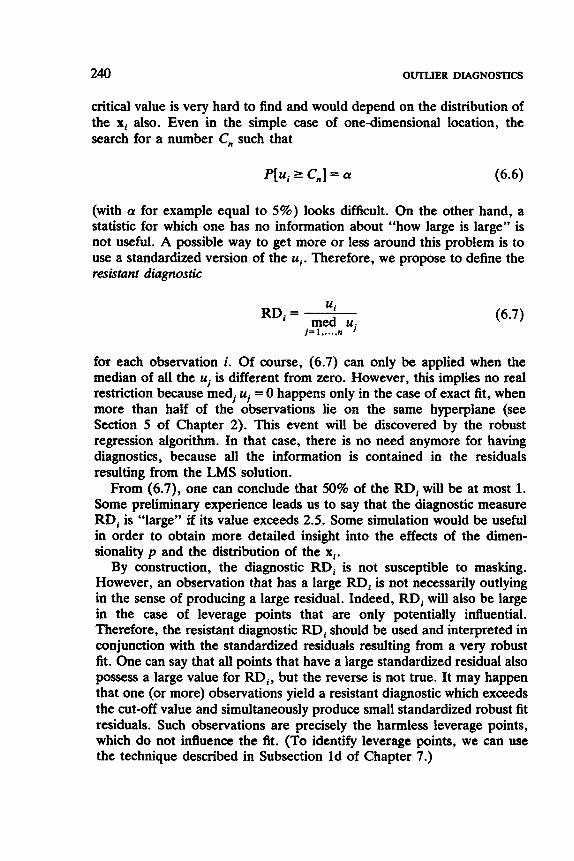
240 OUTLIER DIAGNOSTICS
critical value is very hard to find and would depend on the distribution of the xi also. Even in the simple case of one-dimensional location, the search for a number C,, such that
(with a for example equal to 5%) looks difficult. On the other hand, a statistic for which one has no information about “how large is large” is not useful. A possible way to get more or less around this problem is to use a standardized version of the ui. Therefore, we propose to define the resistant diagnostic
ui RD, = med ui
j-1, ..., n
for each observation i . Of course, (6.7) can only be applied when the median of all the ui is different from zero. However, this implies no real restriction because medj uj = 0 happens only in the case of exact fit, when more than half of the observations lie on the same hyperplane (see Section 5 of Chapter 2). This event will be discovered by the robust regression algorithm. In that case, there is no need anymore for having diagnostics, because all the information is contained in the residuals resulting from the LMS solution.
From (6.7), one can conclude that 50% of the RD, will be at most 1. Some preliminary experience leads us to say that the diagnostic measure RD, is “large” if its value exceeds 2.5. Some simulation would be useful in order to obtain more detailed insight into the effects of the dimen- sionality p and the distribution of the x i .
By construction, the diagnostic RD, is not susceptible to masking. However, an observation that has a large RD, is not necessarily outlying in the sense of producing a large residual. Indeed, RD, will also be large in the case of leverage points that are only potentially influential. Therefore, the resistant diagnostic RD, should be used and interpreted in conjunction with the standardized residuals resulting from a very robust fit. One can say that all points that have a large standardized residual also possess a large value for RD,, but the reverse is not true. It may happen that one (or more) observations yield a resistant diagnostic which exceeds the cut-off value and simultaneously produce small standardized robust fit residuals. Such observations are precisely the harmless leverage points, which do not influence the fit. (To identify leverage points, we can use the technique described in Subsection Id of Chapter 7.)

HIGH-BREAKDOWN DIAGNOSTICS 241
Furthermore, the resistant diagnostic can also be used for determining a weight for each observation by means of a weight function as in (6.1) but with Irila*l replaced by RD,. These weights can then be used for performing a reweighted least squares (RLS). One is sure that at least half of the weights will be 1. In contrast with RLS with weights based on the LMS, this solution will always be unique. A situation where the problem is acute is sketched in Figure 1. The points are generated in the neighborhood of two different lines. Five points satisfy yi = xi + 1 + e,, ei - N(0,l) and the other five points satisfy yi = -xi + 11 + e,, ei - N(0,l). The RLS with weights based on the RD, will yield an inter- mediate but unique solution, which almost bisects the two lines. On the other hand, the LMS will hesitate between both lines and will finally choose one of them. However, the other line also fits about half of the observations. This rather extreme situation in fact poses a new problem. The data set in Figure 1 is not well-fitted by one linear fit but rather by two lines. In this sense it has more to do with cluster analysis (in a framework of linear clusters) than with regression analysis. There exists some literature concerning this so-called two-line regression problem, namely Lenstra et al. (1982) and Kaufman et al. (1983). Because of such ambiguous situations, D. Hoaglin (personal communication) proposed to look also at the second best local minimum of rned,lri(6)l when comput- ing the LMS.
10
9
8
7
6
5
4
3
2
1. Data set illustrating the two-line regression problem.

242 OUTLIER DIAGNOSTICS
The resistant diagnostic is just a by-product of our algorithm for robust regression, so it does not need additional computation time. Therefore, the RD, is also incorporated in PROGRESS and can be obtained by answering yes to the question
W YOU WANT TO COMPUTE OUTLIER DIAGNOSTICS? PLEASE ANSWER YES OR NO:
in the interactive input. The information provided by the resistant diagnostic will now be
illustrated on some examples. The last column of Table 4 contains the RD, values for the Hertzsprung-Russell data. We see that the large RD, values are assigned to the giant stars, which also received a zero weight on the basis of the standardized LMS residuals.
The same observation can be made for the telephone data. In Table 5 we see that the magnitude of RD, is strikingly large for the years 1964-1970.
Table 6 contains the resistant diagnostic values for the first 14 cases of the Hawkins-Bradu-Kass data. (The other cases all possess a small RD, value.) It is not surprising that the 14 printed values are all rather large. The RD, diagnostic measures the outlyingness in x-space as well as the deviation from the fit. Therefore, the good leverage points (11-14) also receive a large RD, value, although they are not regression outliers. From the LMS standardized residuals we know that only the first 10 cases have to be considered as regression outliers.
The RD, for the widely studied Mickey et al. data set are listed in Table 7. Our RD, exceeds the cut-off value 2.50 for the cases 2 and 18. These observations possess small LMS residuals. From both diagnostics together we learn that 2 and 18 are good leverage points. Case 19 (which received a zero weight from LMS) also possesses a relatively large RD, value (1.803) compared to the others.
Let us now briefly compare the diagnostics discussed in this chapter. It seems that an entirely real example with “messy” data might not be completely convincing because we might ecd up with different results without a conclusive way to decide which analysis is best, possibly causing some debates. Therefore, we start with a real data set that is rather well behaved and contaminate it by replacing a few observations. We selected a data set containing 20 points with six parameters to be estimated. The raw data came from Draper and Smith (1966, p. 227) and were used to determine the influence of anatomical factors on wood specific gravity, with five explanatory variables and an intercept. (Draper and Smith conclude that x2 could be deleted from the model, but this matter is not

HIGH-BREAKDOWN DIAGNOSTICS 243
considered for the present purpose.) Table 8 lists a contaminated version of these data, in which a few observations have been replaced by outliers.
A collection of results for these data is given in Table 9. Each column shows a different diagnostic. Entries that exceed a cut-off value (possibly in absolute value) are underlined. Applying LS regression to these data yields
y = 0.4407~, - 1 . 4 7 5 ~ ~ - 0.2612~~ + 0.0208~~ + 0 .1708~~ + 0.4218.
It is not easy to spot the outliers just by looking at the observations, and the standardized LS residuals in Table 9 are of little help. Indeed, the standardized LS residuals look very inconspicuous, except perhaps for observation 11. (Unfortunately, this is a false trail!) Because of this, many people would probably be satisfied with the LS fit (especially when not expecting trouble). The studentized and jackknifed residuals in Table 9 (which are based on LS) also point to case 11. The diagonal elements of the hat matrix are all smaller than the cut-off value 2pln (which equals
Table 8. Modifd Data on Wood Specific Gravity
Index
1 2 3 4 5 6 7 8 9 10 11 12 13 14 15 16 17 18 19 20
X1
0.5730 0.6510 0.6060 0.4370 0.5470 0.4440 0.4890 0.4130 0.5360 0.6850 0.6640 0.7030 0.6530 0.5860 0.5340 0.5230 0.5800 0.4480 0.4170 0.5280
x2
0.1059 0.1356 0.1273 0.1591 0.1135 0.1628 0.1231 0.1673 0.1182 0.1564 0.1588 0.1335 0.1395 0.1114 0.1143 0.1320 0.1249 0.1028 0.1687 0.1057
x3
0.4650 0.5270 0.4940 0.4460 0.5310 0.4290 0.5620 0.4180 0.5920 0.6310 0.5060 0.5190 0.6250 0.5050 0.5210 0.5050 0.5460 0.5220 0.4050 0.4240
0.5380 0.5450 0.5210 0.4230 0.5190 0.4110 0.4550 0.4300 0.4640 0.5640 0.4810 0.4840 0.5190 0.5650 0.5700 0.6120 0.6080 0.5340 0.4150 0.5660
0.8410 0.8870 0.9200 0.9920 0.9150 0.9840 0.8240 0.9780 0.8540 0.9140 0.8670 0.8120 0.8920 0.8890 0.8890 0.9190 0.9540 0.9180 0.9810 0.9090
Y
0.5340 0.5350 0.5700 0.4500 0.5480 0.4310 0.4810 0.4230 0.4750 0.4860 0.5540 0.5190 0.4920 0.5170 0.5020 0.5080 0.5200 0.5060 0.4010 0.5680
Source: Draper and Smith (1966) and Rousseeuw (1984).

Tab
le 9
. D
iagn
ostic
s fo
r the
Dat
a in
Tab
le 8
[h,,;
Squ
ared
Mah
alan
obis
Dis
tanc
e; S
tand
ardi
zed,
Stu
dent
ized
, and
Jac
kkni
fed
LS
Residuals; C
DZ
(i),
DFF
FIIS
, D
FBE
TA
S, S
War
diz
ed L
MS
Res
idua
ls,
and
RD
,]'
~
Bas
ed o
n LS
Rob
ust
r,ls
RD,
DFB
ET
AS (0.447)
Inde
x hi
, M
DT
r,/s
r,
f(i)
C
D2
(i)
DFF
ITS
i (0
.600
) (11.07)
(2.50)
(2.50)
(2.50)
(1.ooO)
(1.095)
Con
st.
8,
4 e,
9, es
(2.50)
(2.500)
1 0.278
4.327
-0.73
-0.85
-0.84
0.047
-0.524
-0.347
-0.004
0.055
0.328
-0.052
0.215
-0.16
0.798
2 0.132
1.552
0.05
0.05
0.05
0.ooO
0.019
-0.o
Cn
0.00
9 0.
W
-0.0
05
0.00
2 O.
Oo0
0.00
0.701
3 0.220
3.224
1.24
1.41
1.46
0.093
0.776
-0.356
-0.651
-0.523
-0.206
-0.429
0.549
0.55
0.577
4 0.258
3.959
0.35
0.41
0.40
0.010
0.236
-0.074
0.035
-0.049
0.015
-0.105
0.118
-14.79
3.9
38
6 0,259
3.974
-0.45
-0.53
-0.51
0.016
-0.302
0.050
-0.053
0.037
0.035
0.130
-0.113
-17.68
4.5
20
8 0.
289
4.536
-0.03
-0.04
-0.04
O.Oo
0 -0.025
-0.005
0.011
-0.012
0.005
-0.005
0.00
6 -1
7.31
4.466
9 0.348
5.665
-0.40
-0.49
-0.48
0.021
-0.348
-0.075
0.052
0.105
-0.224
0.161
0.00
7 -0.73
1.243
10
0.449
7.588
-0.42
-0.56
-0.55
0.043
-0.492
0.257
-0.008
-0.198
-0.256
-0.137
-0.0
29
-0.40
1.267
5 0.223
3.271
1.00
1.14
1.15
0.062
0.615
-0.244
0.286
-0.$17
0.164
-0.388
0.437
1.75
0.605
7 0.530
9.124
0.91
1.32
1.36
0.329
1.448
1.027
-0.9
56
0.424
0.521
0.133
-0.9
64
0.73
1.421
11
0.317
5.075
1.99
2.40
3.(n
0.447
2.059
0.5
21
0.425
0.748
0.198
-0.8
oO
0.00
1.258
12
0.410
6.833
-1.20
-1.56
-1.65
0.281
-1.376
-0.566
-0.597
0.013
o.u6
0.359
0.36
8 -1.88
1.030
13
0.28
7 4.506
-0.49
-0.58
-0.56
0.02
2 -0.356
0.180
-0.098
0.045
-0.251
0.106
-0.121
0.00
1.015
14
0.129
1.5M)
-1.26
-1.35
-1.40
0.045
-0.537
0.021
-0.169
0.22
8 0.178
-0.0
06
-0.103
-1.30
0.66
8 15
0.152
1.945
-0.5
9 -0.64
-0.62
0.012
-0.264
-0.073
0.148
-0.061
-0.011
-0.162
0.108
-0.34
0.465
16
0.52
6 9.049
0.52
0.76
0.75
0.107
0.789
0.122
-0.5
29
-0.0
52
0.745
-0.432
0.00
0.865
17
0.28
9 4.548
-0.25
-0.30
-0.29
0.00
6 -0.187
0.133
-0.019
0.019
-0.044
-0.055
-0.086
0.00
0.80
2 18
0.294
4.637
0.28
0.34
0.33
0.00
8 0.211
-0.002
-0.062
-0.096
0.081
-0.024
0.045
-0.21
0.985
19
0.292
4.599
-1.08
-1.29
-1.32
0.114
-0.849
-0.128
0.195
-0.287
0.231
-0.024
0.07
9 -2
0.84
5.201
20
0.318
5.084
0.S
0.66
0.65
0.034
0.441
0.06
4 0.
092
-0.154
-0.305
0.037
0.04
6 0.00
0.816
The
cut
-off
val
ue f
or h
,, is
Zp
/n =
0.6
00, a
nd fo
r M
Df
it is
9s =
11.
07.

EXERCISES AND PROBLEMS 245
0.6). Also, CD2(i) is less than 1 everywhere. The single-case diagnostics DFFITS, and in part also DFBETAS, point to observations 7, 11, and 12. The cases 3, 5, and 16 also show some values of DFBETAS which are larger than 2/t/7i (which equals 0.447). However, none of these diagnos- tics have succeeded in identifying the actual contaminated cases. Let us now examine the column with the standardized residuals associated with the LMS fit
y^= 0 .2687~~ - 0 . 2 3 8 1 ~ ~ - 0 . 5 3 5 7 ~ ~ - 0 . 2 9 3 7 ~ ~ + 0 . 4 5 1 0 ~ ~ + 0.4347.
These standardized residuals make it easy to spot the four outliers. Indeed, the cases with indices 4, 6, 8, and 19 are the contaminated ones. The resistant diagnostic confirms the conclusions drawn from the standar- dized LMS residuals. In this example, the outliers are bad leverage points that are not outlying in any of the individual variables, as in Figure 4 of Section 1 in Chapter 1. Note that neither the hat matrix nor any other classical diagnostic is able to detect this fact, because they are susceptible to the masking effect (which is just another way of saying that they have a low breakdown point).
Our last example is the stackloss data set (Table 1 of Chapter 3). From Table 10, we see that this is relatively easy, because the different diagnostics lead to more or less the same conclusions. The LS residuals are largest (but not very large) for observations 1, 3, 4, and 21. The DJ?FITS and DFBETAS diagnostics exceed their cut-off values for case 21. The DFFITS value approaches the cut-off for cases 1, 3, and 4. The 17th diagonal element of the hat matrix slightly surpasses 2pln = 0.381, so it may be considered a good leverage point. The outlying cases 1,3,4, and 21 are detected by both the LMS residuals and the resistant diagnos- tic RD,.
EXERCISES AND PROBLEMS
Section 2
1. Show that the hat matrix H defined in (2.3) is idempotent (HH=H) and symmetric (H' = H).
section 3
2. Prove the alternative formulas (3.3) and (3.4) of Cook's squared distance.

Tab
le 1
0. D
iagn
ostic
s A
ssoc
iate
d w
ith t
he S
tack
low
Dat
a [h
,,; S
quar
ed M
ahaJ
anob
is D
ista
nce;
Sta
ndar
dize
d, S
tude
ntiz
ed, a
nd
Jack
knife
d LS R
esid
uals
; CD
'(I);
DFF
ITS;
DFB
ET
AS;
Sta
ndar
dize
d L
MS
Res
idua
ls; RD,]
Bas
ed o
n LS
Rob
ust
rils
R
D,
DF
BE
TA
S (0
.436
) In
dex
h,,
MD
: ri
/s
ti
t(i)
CD
2(i)
D
FFIT
S i
(0.3
81)
(7.8
2)
(2.5
0)
(2.5
0)
(2.5
0)
(1.O
OO
) (0
.873
) C
onst
. 6,
4
0, (2
.50)
(2
.500
)
1
2 3 4 5 6 7 8 9 10
11
12
13
14
15
16
17
18
19
20
21
0.302
0.31
8 0.
175
0.12
9 0.
052
0.07
8 0.
219
0.21
9 0.
140
0.20
0 0.
155
0.21
7 0.
158
0.20
6 0.
191
0.13
1
0.16
1 0.
175
0.08
0
5.07
9 5.
404
2.54
0 1.
618
0.09
2 0.
597
3.43
2 3.
432
1.85
1 3.
049
2.14
8 3.
391
2.19
8 3.
164
2.85
7 1.
669
7.29
0 2.
260
2.53
8 0.
651
1.00
1.
19
1.21
-0
.59
-0.7
2 -0
.71
1.40
1.
55
1.62
1.
76
1.88
2.
05
-0.5
3 -0
.54
-0.5
3 -0
.93
-0.9
7 -0
.96
-0.7
4 -0
.83
-0.8
3 -0
.43
-0.4
9 -0
.47
-0.9
7 -1
.05
-1.0
5 0.
39
0.44
0.
43
0.81
0.
88
0.88
0.
86
0.97
0.
97
-0.4
4 -0
.48
-0.4
7 -0
.02
-0.0
2 -0
.02
0.73
0.
81
0.80
0.
28
0.30
0.
29
-0.4
7 -0
.61
-0.60
-0.1
4 -0
.15
-0.1
5 -0
.18
-0.2
0 -0
.20
0.44
0.
45
0.44
0.15
4 0.060
0.12
6 0.
131
0.00
4 0.
020
0.04
9 0.
017
0.04
5 0.
012
0.03
6 0.
065
0.01
1 O.
OO0
0.03
9 0.
003
0.06
5 0.
001
0.002
0.00
4
0.79
5 -0
.481
0.
744
0.78
8 -0
.125
-0
.279
-0
.438
-0
.251
-0
.423
0.
213
0.37
6 0.
509
-0.2
03
-0.0
09
0.38
8 0.
113
-0.5
02
-0.0
65
-0.0
91
0.13
1
-0.0
85
0.01
3 -0
.188
-0
.122
0.
012
0.03
9 0.
296
0.16
9 0.
077
0.15
3 -0
.068
-0
.011
-0
.119
0.
005
-0.1
16
O.OO
0 -0
.462
-0
.047
-0
.049
0.
085
0.400
-0.2
50
0.39
1 -0
.415
0.
012
0.10
6 0.
268
0.15
4 0.
307
0.12
4 0.
108
0.23
3 -0
.116
-0
.001
-0
.195
-0
.053
0.
020
0.02
3 0.
052
-0.0
11
0.10
3 -0
.061
-0
.005
0.619
-0.0
30
-0.1
69
-0.2
63
-0.1
51
-0.3
28
-0.1
32
-0.2
65
-0.4
27
0.14
1 0.
003
-0.0
29
-0.0
10
-0.0
63
-0.0
13
-0.0
42
0.00
5
-0.2
10
0.16
5 -0
.047
0.
027
-0.007
-0.0
12
-0.2
82
-0.1
62
-0.0
78
-0.1
28
0.15
8 0.
128
0.08
8 -0
.007
0.
247
0.04
2 0.
424
0.03
3 0.
034
-0.0
67
7.7
0-
3.7
4 1.
5%
7.1
43
.04
7
m3.265
0.28
0.
617
0.00
0.
821
0.51
1.m
1.
30
0.89
2 -0
.11
0.86
0 0.
51
1.27
5 0.
51
0.84
2 0.
00
1.04
4 -1
.87
1.01
8 -1
.36
0.90
2 0.
28
0.990
-0.5
1 0.
700
0.00
2.
137
0.00
1.
146
0.51
0.
941
1.87
0.
806
0.28
5 4.
738
-2.2
3 -2
.64
-3.3
3 0.
692
-2.1
00
0.402
-1.6
24
1.64
2 -0
.363
-6
.06
2.854

EXERCISES AND PROBLEMS 247
3. How many outliers does it take to make the diagnostics of Sections 2 and 3 unreliable? Consider the following procedure: First delete all points for which a classical diagnostic exceeds its cut-off, then apply LS on the remaining data. What is the breakdown point of this two-stage estimator?
4. There are basically three kinds of outlier diagnostics: those that aim at identifying outliers in y, those that try to find leverage points (whether they are good or bad), and the combined diagnostics that look for both leverage points and outliers in y. In which category are the hi,, ri/s, MD:, CD2(i) , and DFFITS?
Section 6
5. Try to find the leverage points of the data in Table 8 by making all scatterplots between any two explanatory variables. Do you think it is always possible to discover the leverage points in this way?
6. Consider again the aircraft data listed in Table 22 of Chapter 3. Run PROGRESS with the diagnostics option, and discuss the hii and RD, together with the residuals of Ls, LMS, and RLS to distinguish between good and bad leverage points. Compare these results with the analysis of Gray (1985), who uses diagnostic graphics, and with any other diagnostics that may be available in your local statistical software.
7. Analyze the delivery time data (exercise 2 of Chapter 3) by running PROGRESS with the diagnostics option. For which cases is hi,> 2p/n? Explain the masking effect by comparing with the hi, in the RLS output, where the bad leverage point has been deleted. Also discuss the robustly standardized residuals and the resistant diagnostic RD,.
8. Use the hi, to discover the leverage point in the phosphorus content data (Table 24 of Chapter 3). Should you look at the LS or the LMS residuals to find out whether it is a good or a bad leverage point? Also discuss the resistant diagnostic RD, in this example, as well as any other diagnostics provided by your local software.

C H A P T E R 7
Related Statistical Techniques
The preceding chapters all dealt with high-breakdown methods in regres- sion analysis (including the special case of one-dimensional location). However, the same ideas can also be applied to other statistical proce- dures. In the first section of this chapter we shall focus our attention on multivariate location and covariance, a topic which is itself a key to various statistical techniques. Section 2 is about robust time series analysis, and Section 3 briefly discusses the merits of robustification in other situations.
1. COVARIANCE MATRICES, INCLUDING THE DETECTION OF LEVERAGE POINTS
ROBUST ESTIMATION OF MULTIVARIATE LOCATION AND
Outliers are much harder to identify in multivariate data clouds than in the univariate case. Therefore, the construction of robust techniques becomes more difficult. We shall focus on the estimation of the “center” of a point cloud, in which all variables are treated in the same way (unlike regression analysis, where one tries to “explain” one variable by means of the remaining ones). We are also interested in the dispersion of the data about this “center.”
Suppose we have a data set
x= {XI,. . . , x,}
= {(XI], x12, - - 9 XIp), * * - 9 G , I , X n 2 , * - 7 -GP)} (1.1)
of n points in p dimensions, and we want to estimate its “center.” (We have decided to denote the cases by rows, to keep the notation consistent
248
Robust Regression and Outlier Detection Peter J. Rousseeuw, Annick M. Leroy
Copyright 0 1987 John Wiley & Sons, Inc. ISBN: 0-471-85233-3

ROBUST ESTIMATION OF MULTIVARIATE LOCATION 249
with previous chapters.) For this purpose, we apply a multivariate location estimator, that is, a statistic T which is translation equivuriant,
T(x, + b, . . . , x, + b) = T(xl, . . . , x,) + b , (1.2)
for any p-dimensional vector b. This property is also referred to as location equivuriance. Naturally, T also has to be permutation invariant,
for any permutation w on {1,2, . . . , n } . Of course, not every such Twill be useful, and additional conditions
may be required, depending on the situation. The most well-known estimator of multivariate location is the arithmetic mean
which is the least s uares estimator in this framework because it mini- mizes E:=] llxi - TI1 , where 11 - . - I 1 is the ordinary Euclidean norm. However, it is well known that 5 is not robust, because even a single (very bad) outlier in the sample can move 5 arbitrarily far away. To quantify such effects, we slightly adapt the finite-sample breakdown point of Section 2 in Chapter 1 to the framework of multivariate location. We consider all corrupted samples X' obtained by replacing any m of the original data points by arbitrary values, and we define the maximal bias
4
by
bias (m; T, X ) = sup 11 T ( X ) - T(X)ll (1.5) X'
so the breakdown point
E: (T, X) = min { m/n; bias (m; T , X ) is infinite} (1.6)
is again the smallest fraction of contamination that can cause T to take on values arbitrarily far away. Obviously, the multivariate arithmetic mean possesses a breakdown point of l ln . (Therefore, it is not well suited for the detection of outliers, as will be seen in Subsection d below.) We often consider the limiting breakdown point for n + m , so we say that the multivariate mean has 0% breakdown.
It is clear that no translation equivariant T can have a breakdown point larger than 50%, because one could build a configuration of outliers

250 RELATED STATISTICAL TECHNIQUES
which is just a translation image of the “good” data points, making it impossible for T to choose. In one dimension, this upper bound of 50% can easily be attained, for instance, by the sample median. Therefore, several multivariate generalizations of the median have been con- structed, as well as some other proposals to achieve a certain amount of robustness.
Before listing some of these robust alternatives, we shall distinguish between two classes of location estimators: those that are affine equivariant and those that are not. Indeed, in many situations one wants the estimation to commute with linear transformations (i.e. , a reparamet- rization of the space of the xi should not change the estimate). We say that T is afine equivariant if and only if
T(x,A +by. . . , x,A + b) = T ( x l , . . . , x,)A + b
for any vector b and any nonsingular matrix A. (Because xi and T are denoted by rows, the matrix A has to stand on the right.) For instance, the arithmetic mean does satisfy this property, but not all robust es- timators do. We shall first consider some nonequivariant proposals.
a. Robust Estimators That Are Not Afline Equivariant
The simplest idea is to consider each variable separately. Indeed, for each variable j the numbers x l j , x y r . . . , xnj can be considered as a one- dimensional data set with n points. One may therefore apply a univariate robust estimator to each such “sample” and combine the results into a p-dimensional estimate. This procedure inherits the breakdown point of the original estimator.
For instance, the coordinatewise median is defined as
(med x i , , med xi2 , . . . , med x i p ) 1
and possesses a 50% breakdown point. This estimator is easily computed, but fails to satisfy some “natural” properties. For instance, it does not have to lie in the convex hull of the sample when p 2 3. As an example, consider the p unit vectors ( l , O , . . . ,O), ( O , l , . . . ,O),.. . , (O,O, . . . , l), the convex hull of which is a simplex not containing the coordinatewise median (0, 0, . . . , 0). (However, it does lie in the convex hull when p I 2, as can be shown by a geometrical argument.)
Nath (1971) proposed another coordinatewise technique, in which each component is investigated separately, and a certain fraction of the largest and the smallest observations are not used. This method is very

ROBUST ESTIMATION OF MULTIVARIATE LOCATION 251
simple, but many outliers may go unnoticed because multivariate outliers do not necessarily stick out in any of their components (see Figure 4 of Chapter 1).
Note that the multivariate arithmetic mean, although affine equivariant, can also be computed coordinatewise. However, thib is an exception. Indeed, Donoho (1982, Proposition 4.6) showed that the only (measurable) location estimator that is both affine equivariant and computable as a vector of one-dimensional location estimators is the arithmetic mean.
Sometimes one does not wish equivariance with respect to all affine transformations, but only for those that preserve Euclidean distances, that is, transformations of the t e x--, xi’ + b where r is an orthogonal matrix (this means that I” = r- ). This includes translations, rotations, and reflections. For instance, the L, location estimator, given as the solution T of
YP
is orthogonal equivariant, because the objective function only depends’ on Euclidean distances. In operations research, this estimate is called the Weber point, and it corresponds to the optimal location to build a factory when the customers sit at the xi and the total transportation cost is to be minimized. Several routines are available to compute T. The L, estimator is also a generalization of the univariate median, and its breakdown point is still 50%. (Some people call it the “spatial median” or the “median center.”)
Orthogonal equivariant estimators are often used to estimate the center of a spherically symmetric density
fJx) = d l l x - PII) - (1.10)
This symmetry assumption may be reasonable when the data are points in some physical space (such as the customers in industrial location, or stars in three-dimensional space), but one should be careful when applying such procedures to variables of different types, in which case the choice of measurement units becomes important. For instance, when the vari- ables are height and time, it makes a lot of difference whether these are expressed in feet and minutes or in centimeters and hours. (In such situations, it may be safer to apply either coordinatewise techniques or affine equivariant ones.)
When the spherically symmetric density is Gaussian, the maximum
252 RELATED STATISTICAL TECHNIQUES
likelihood estimator becomes the arithmetic mean. This suggests a (mod- est) generalization of M-estimators, given by
n
Minimize p( llxi - TI]) . ' i=1 (1.11)
Huber (1967) considered the asymptotic behavior of these estimators, and Collins (1982) obtained some results on minimax variance.
b. AflRw Equivariant Estimators
Let us now consider estimators that do satisfy the affine equivariance condition. Such estimators are particularly useful in a model with so- called elliptical symmetry, with density
Pet (A)rdlI (x - P>A-'ll> * (1.12)
This model is obtained when starting from a spherically symmetric density, to which an affine transformation is applied. Unfortunately, the pair ( p, A) is not a suitable parametrization because both A and r A (with orthogonal I') lead to the same distribution. However, the symmetric and positive definite matrix Z = A'A is the same for all A leadin to the same density, because II(x - p)A-'Il= [(x - p)(A'A)-'(x - p)']'! Therefore, we parametrize the model as
f,.,(x) = (det (Z))-"*g([(x - p)Z-'(x - p)']"') . (1.13)
The typical example is the multivariate normal distribution N( p, 8), where Z is the (variance-) covariance matrix. Therefore, 8 is called a (pseudo-) covariance matrix, or scatter matrix, even in the general situation. Both p and P must be estimated. For covariance estimators, affine equivariance means that
C({x,A + b, . . . , x,A + b}) = A'C({x,, . . . , xn})A , (1.14)
where A is any nonsingular p-by-p matrix and b is any vector. At N( p, X), maximum likelihood yields the equivariant estimators
(1.15) 1 "
T ( X ) = Z and C ( X ) = ; 2 (xi - Z)'(xi - Z) i = l
(to obtain an unbiased estimator of 8, the denominator of C(X) must be replaced by n - 1).
ROBUST ESTIMATION OF MULTIVARIATE LOCATION 253
In order to generalize the maximum likelihood approach, Hampel (1973) suggested an affine equivariant iterative procedure to estimate p and 2. Maronna (1976) formally introduced affine equivariant M- estimators of location and scatter, defined as simultaneous solutions of systems of equations of the form
1 " n
1 "
- c UI([(Xi - T)c-'(x, - T)']''*)(Xi - T ) = 0
- c U& - T)c-'(x, - T)')(x, - T)'(x, - T ) = c , (1.16) 1 n i - I
where uI and u2 must satisfy certain assumptions, and he considered the problems of existence, uniqueness, consistency, and asymptotic normali- ty. Huber (1977, 1981) and Stahel (1981) computed influence functions and showed that the breakdown point of all affine equivariant M- estimators is at most l l ( p + l), which is disappointingly low. In a numerical study, Devlin et al. (1981, p. 361) found that M-estimators could tolerate even fewer outliers than indicated by this upper bound. Recently, Tyler (1986) found that the estimated scatter matrix becomes singular (which is a form of breaking down) when the contaminated data lie in some lower-dimensional subspace.
Affine equivariant M-estimators can be computed recursively, for instance by means of ROBETH (Marazzi 1980) or COVINTER (Dutter 1983b). A survey of affine equivariant M-estimators can be found in Chapter 5 of Hampel et al. (1986), and some recent results are given by Tyler (1985a,b).
Donoho (1982) lists some other well known affine equivariant tech- niques and shows that they all have a breakdown point of at most l l(p + 1). These proposals include:
1. Convex Peeling (Barnett 1976, Bebbington 1978; based on an idea of Tukey). This proceeds by discarding the points on the boundary of the sample's convex hull, and this is repeated until a sufficient number of points have been peeled away. On the remaining data, classical es- timators can be applied. This procedure appeals to the intuition, and it is indeed equivariant because the convex hull is preserved by affine trans- formations. However, the breakdown point is quite low (even when the "good" data come from a multivariate normal distribution) because each step of peeling removes at least p + 1 points from the sample, and often only one of these is really an outlier, so the stock of "good" points is being exhausted too fast.
2. Ellipsoidal Peeling (Titterington 1978, Helbling 1983). This is simi-

254 RELATED STATISTICAL TECHNIQUES
lar to convex peeling, but removes all observations on the boundary of the minimum volume ellipsoid containing the data. (Note that the convex hull is also the smallest convex set containing all the points.) Affine transformations x+ xA + b map ellipsoids onto ellipsoids, and the vol- ume of the image is just ldet (A)I times the original volume, so ellipsoidal peeling is again affine equivariant. However, its breakdown point also tends to 1/( p + 1) for the same reasons.
3. Classical Outlier Rejection. The (squared) Mahalanobis distance
MD~(x,, x) = (xi - T(x))c(x)-’(x, - ~ ( x ) ) ‘ (1.17)
is computed for each observation, where T ( X ) is the arithmetic mean and C(X) is the classical covariance estimate (1.15) with denominator n - 1 instead of n. Points for which MD2(x,, X) is large are deleted from the sample, and one processes the “cleaned” data in the usual way. (The result will be affine equivariant because the MD2(xi, X) do not change when the data are subjected to an affine transformation,) This approach works well if only a single outlier is present (Barnett and Lewis “78, David 1981), but suffers from the masking effect otherwise, because one far-away outlier can make all other outliers have small MD2(xi, X). (In other words, the breakdown point is only 2/n.) Therefore, some refine- ments of this technique have been proposed.
4. Iterative Deletion. This consists of finding the most discrepant observation according to (1.17), deleting it, recomputing T ( X ) and C(X) for the remaining data and using it to find the most discrepant xi among those n - 1 points, and so on. Several rules are possible to decide how many observations are to be removed, but at any rate the breakdown point of the mean of the remainder can be no better than I/( p + 1).
5. Iterative Trimming (Gnanadesikan and Kettenring 1972, Devlin et al. 1975). This starts with X ( l ) = X and defines X(’+’) recursively as the set of observations with the (1 - a)n smallest values in {MD2(x,, . . . all have the same number of points.) This iterative process is halted when both T(X‘&)) and C(X‘”) stabilize. By means of a heuristic reasoning, Donoho (1982) concluded that the breakdown point of the final T ( X ) is at most about
6. Depth Trimming. This is based on the concept of depth (Tukey 1974), which provides a kind of “rank statistic” for multivariate data sets. The depth of xi is the smallest number of data points in any half-space containing it. Donoho (1982) defines a depth-trimmed mean as the average of all points with depth at least k. The higher the k , the better
xi E X}. (Note that X‘”,
l l p .

ROBUST ESTIMATION OF MULTIVARIATE LOCATION 255
the resulting breakdown point will be. The trimmed mean with k = maxi depth ( x i ) , which may be called the deepest points estimator, generalizes the univariate sample median. Unfortunately, not all data sets contain very deep points. In fact, Donoho proves that the maximal depth (in any data set) satisfies
[n/( p + l)] 5 maxi depth ( x i ) I [n/2] . Both bounds are sharp. The upper bound is achieved when there is a point about which the sample is centrosymmetric, and then the break- down point of the deepest points estimator is about 1/3. On the other hand, the lower bound is reached when the data are evenly distributed over small clusters on the p + 1 vertices of a simplex, in which case the breakdown point of any depth-trimmed mean is at most 1/( p + 2).
Recently, Oja (1983) has put forward another affine equivariant proposal, which he calls the generalized median. It is defined by minimi- zation of
(1.18)
where the summation is over 1 I i, < - - < i,, 5 n, and A(xi,, . . . , xip, T ) is the volume of the simplex with vertices xi , , . . . , xip and T. Figure 1 illustrates the meaning of (1.18) in two dimensions: Instead of minimizing the total length of the lines linking T to each data point [as in (1.9), the spatial median], we now minimize the total area of all triangles formed by T and any pair of data points.
This is already the fourth generalization of the univariate median that we encounter. Like Donoho’s deepest points estimator, also Oja’s generalized median is affine equivariant. Indeed, any affine transforma- tion x+ xA + b merely multiplies the volumes A(xi,, . . . , xip, T ) by the constant factor ldet (A)I, which is immaterial to the minimization. How- ever, this equivariance costs a lot, because the algorithm mentioned by Oja and Niinimaa (1985) for computing T ( X ) appears to involve the computation of the objective function (1.18), which contains C: terms, in each of
A(xil, . . . , xip , T) ,
c;: candidate estimates. Oja and Niinimaa (1985) showed that the general- ized median is asymptotically normal, with good statistical efficiency. It was recently found that the breakdown point equals 1 /3 in the bivariate case, and it is assumed that in thep-variate case it is I / ( p + 1) (Oja 1986,

256 RELATED STATISTICAL TECHNIQUES
Figure 1. An illustration of Oja’s generalized median, which minimizes the total area of all triangles formed with any pair of observations. (Not all such triangles are drawn.)
personal communication). Brown and Hettmansperger (1985) constructed affine invariant bivariate rank tests based on this estimator. To conclude, all these affine equivariant estimators are facing the
ubiquitous upper bound 1/( p + 1) on their breakdown point. Fortunate- ly, affine equivariant estimators with a higher breakdown point have recently been introduced.
c. Afline Equivariant Methods with High Breakdown Point
The first affine equivariant multivariate location estimator with a 50% breakdown point was obtained independently by Stahel (1981) and Donoho (1982). This estimator, called ourzyingness-weighred mean, is defined as follows. For each observation x i , one looks for a one- dimensional projection leaving it most exposed. This is done by comput- ing the following measure of the “outlyingness” of x i :
ll,.llL1 med ( X k v ‘ - med (xjv‘)/ ’ Ixiv‘ - med (xjv‘)I
(1.19) I ui= sup k I

ROBUST FSTIMATION OF MULTIVARIATE LOCATION 257
where medj (xjv') is the median of the projections of the data points xi on the direction of the vector v, and the denominator is the median absolute deviation of these projections. To compute ui, one must (in principle) search over all possible directions. Then one estimates location by the weighted mean
(1.20)
E w(ui) i = l
where w(u) is a strictly positive and decreasing function of u 1 0 , such that uw(u) is bounded. [The latter bound is dictated by the one- dimensional case, where (1.20) reduces to a one-step W-estimator starting from the median (Hampel et al. 1986, p. 116), the influence function of which is proportional to uw(u).] Analogously, these weights can also be used to compute a robust covariance matrix.
Donoho (1982) motivates (1.19) by noting that the classical (squared) Mahalanobis distance (1.17) can also be written as
which is quite vulnerable to outliers, because they affect
9 (1.21)
both the mean (l /n) C~~l-x,v' and the standard deviation SD (x,v', . . . , x,v') of the projected data. Therefore it seems natural to replace these by robust estimators such as the median and the median absolute deviation, where- as Stahel (1981) proposed to insert also other univariate M-estimators. Points with large ui are unlikely to belong to the "good" data, so their downweighting makes sense. It is shown that (1.20) is affine equivariant, because the ui do not change when the xi are transformed to xiA + b. Donoho (1982) also showed that the breakdown point of (1.20) is high (supposing that n is larger than 2p + 1) and tends to 50% for n + 00. In his proof, he assumed that X is in general position, which, in the context of multivariate location, means that no more than p points of X lie in any ( p - 1)-dimensional affine subspace. (For two-dimensional data, this says that there are no more than two points of X on any line, so any three points of X determine a triangle with nonzero area.) The asymptotic behavior of this estimator has recently been investigated by Donoho (1986, personal communication).

258 RELATED STATISTICAL TECHNIQUES
The Stahel-Donoho estimator downweights any point that is many robust standard deviations away from the sample in some projection. Therefore, it is related to the projection pursuit principle discussed in Section 5 of Chapter 3. The projections are on one-dimensional sub- spaces, and their “interestingness” is measured by the objective function in (1.19). For each point, the corresponding “least favorable” projection must be found, leading to ui.
Rousseeuw (1983, 1984) introduced a second affine equivariant es- timator with maximal breakdown point, by putting
T ( X ) = center of the minimal volume ellipsoid covering (at least) h points of X , (1.22)
where h can be taken equal to [n/2] + 1. This is called the minimum volume ellipsoid estimator (MVE). The corresponding covariance es- timator is given by the ellipsoid itself, multiplied by a suitable factor to obtain consistency. Affine equivariance of the MVE follows from the fact that the image of an ellipsoid through a nonsingular affine transformation x+ xA + b is again an ellipsoid, with volume equal to ldet (A)l times the original volume. Because ldet(A)I is a constant, the relative sizes of ellipsoids do not change under affine transformations.
Themern 1. At any p-dimensional sample X in general position, the breakdown point of the W E estimator equals
which converges to 50% as n + 00.
Proof. Without loss of generality, let T ( X ) = 0. We put M := volume of the smallest ellipsoid with center zero containing all points of X; Because X is in general position, each of its C,P+’ subsets of p + 1 points (indexed by some J = {il, . . . , i , , , } ) determines a simplex with nonzero volume. Therefore, for each such J there exists a bound d , such that any ellipsoid with center llcll> d, and containing { x i , , . . , , xi } has a volume strictly larger than M. Put d := max, d, < 00.
Let us first show that cz (T, X) 2 ([n/2] - p + l ) /n. Take any sample X’ obtained by replacing at most [n/2]-p points of X. Suppose 11 T(X‘)ll> d , and let E be the corresponding smallest ellipsoid con- taining (at least) [n/2] + 1 points of X’. But then E contains at least ( [ n / 2 ] + 1) - ([n/2] - p ) = p + 1 points of X, so volume(E) > M. This is a contradiction, because the smallest ellipsoid with center zero around the
P + l

ROBUST ESTIMATION OF MULTIVARIATE LOCATION 259
n - ( [n /2 ] - p) L [n/2] + 1 “good” points of X’ has a volume of at most M. Therefore, IIT(X’)I(Sd. [Even if T(X‘ ) is not unique, then 11 T(X,)ll I d still holds for all solutions.] On the other hand, EE(T, X) i ( [n/2] -p + l)/n. Indeed, take any p
points of X and consider the ( p - 1)-dimensional affine subspace H they determine. Now replace [n/2] - p + 1 other points of X by points on H. Then H contains [n/2] + 1 points of the new sample X’, so the minimal volume ellipsoid covering these [n/2] + 1 points degenerates to zero volume. Because X is in general position, no ellipsoid covering another subset of [n/2] + 1 points of X’ can have zero volume, so T(X‘) lies on H. Finally, we note that T(X’) is not bounded because the [n/2] - p + 1 contaminated data points on H may have arbitrarily large norms. 0
In most applications it is not feasible to actually consider all “halves” of the data and to compute the volume of the smallest ellipsoid around each of them. As in the case of least median of squares (LMS) regres- sion, we therefore resort to an approximate algorithm not unlike the one described in Section 1 of Chapter 5. We start by drawing a subsample of ( p + 1) different observations, indexed by J = {i l , . . . , ip+,}. For this subsample we determine the arithmetic mean and the corresponding covariance matrix, given by
where C , is nonsingular whenever xi , , . . . ,x i ,+ , are in general position. The corresponding ellipsoid should then be inflated or deflated to contain exactly h points, which corresponds to computing
m; = med (xi - E,)Cil(xi - Z J ) ‘ ( 1.24)
because m, is the right magnification factor. The volume of the resulting ellipsoid, corresponding to m;C J , is proportional to
i = l , . . . . n
(det (m3CJ))1’2 = (det (CJ))1’2(mJ)p . (1.25)
This has to be repeated for many J, after which the one with the lowest objective function (1.25) is retained. We then compute
(1.26)
where ,y~,o.so is the median of the chi-squared distribution with p degrees

260 RELATED STATISTICAL TECHNIQUES
of freedom. (This correction factor is for consistency at multivariate normal data.) The number of random subsamples J that are needed can be determined as in Section 1 of Chapter 5. Indeed, the probability that at least one out of m subsamples consists exclusively of “good” points is approximately
1 - (1 - (1 - & ) P + y (1.27)
when the original data contains a fraction E of outliers. By imposing that this probability exceeds a given value, one obtains the number rn of replications.
The complexity of this algorithm is similar to that of LMS regression, because for each of the m replications a p-by-p matrix C , must be inverted (this can even be done somewhat faster because C , is symmetric and positive definite). Then a median of the n “squared residuals” must be computed in (1.24). Note that the calculation of det (C , ) does not cost extra, because it is obtained as a by-product of the computation of C;’. Also note that this algorithm is itself affine equivariant and that it may easily be parallelized by treating many subsamples simultaneously.
The (approximate) MVE estimates can also be used as initial solutions on which to base a one-step improvement. As in the case of reweighted least squares regression (see Section 2 of Chapter 1) we can assign a weight wI to each observation by means of the rule
where the cut-off value c might be taken equal to x : , ~ . ~ , ~ . Then one can apply the reweighted estimators
n c wixi i= 1 T l ( X ) = -
i = l
and
(1.29)
c, w i - 1 i = l

ROBUST ESTIMATION OF MULTIVARIATE LOCATION 261
which simply means that the classical computations are carried out on the set of points for which wi = 1.
The above algorithm (both MVE and reweighted) has been imple- mented in a program called PROCOVIEV (Rousseeuw and van Zomeren 1987). This abbreviation stands for Program for Robust Covariance and Identification of Extreme Values, indicating its ability to discover multivariate outliers.
Example Let us consider the Hertzsprung-Russell data of Table 3 of Chapter 2. This time we treat both variables (log temperature and log light intensity) in the same way, so we have 47 points in the plane. Figure 2 shows the classical 97.5% tolerance ellipse, obtained from the usual mean and covariance matrix (dashed line). Note that this ellipse is very big, because it is attracted by the four outliers (indeed, the tolerance ellipse tries to engulf them). On the other hand, the tolerance ellipse based on the MVE estimates (solid line) is much smaller and essentially fits the main sequence. The four giant stars, lying far away from this ellipse, can then be identified as not belonging to the same population as the bulk of the
I I I I ' I I I I 1 1 ' 1
- 1 1 1 1 1 1 1 l 1 1 1 1 1 1 1 1 1 1 ,
5.0 4.8 4.6 4.4 4.2 4.0 3.8 3.6 3.4
Figure 2. Hertzsprung-Russell data of Chapter 2, with 97.5% tolerance ellipse obtained from the classical estimator (dashed line) and based on the MVE estimator (solid line).

262 RELATED STATISTICAL TECHNIQUES
data. Note that choosing other measurement units for the variables would yield essentially the same result, because of affine equivariance. Also note that this analysis is basically different from that presented in Figure 4 of Chapter 2, because there the aim was to write the log light intensity as a linear function of the log temperature, and the LMS tried to find the narrowest strip covering half of the data, whereas we now made use of the smallest elZipse covering half of the data. However, we could con- struct another robust regression line of y on x based on this ellipse, by putting
j7 = f ( x ) = midpoint of the intersections of the vertical line through x with the ellipse
in the same way that the LS line is derived from the classical covariance matrix. This could easily be generalized to multiple regression.
For p = 1 (univariate location) the minimum volume ellipsoid reduces to the shortest half, so T ( X ) becomes the one-dimensional LMS discussed in Chapter 4. In particular, Theorem 3 in Section 4 of Chapter 4 shows that this estimator converges as n-1’3, which is abnormally slow. It is assumed that the multivariate MVE will not have a better rate, so it is useful to perform a one-step reweighting [based on formula (1.28) above] to improve its statistical efficiency. (Alternatively, a one-step M-estimator might be applied.)
Another approach would be to generalize the least trimmed squares (LTS) estimator (which converges like n-l’* according to Theorem 4 in Section 4 of Chapter 4) to multivariate location. This yields
T ( X ) = Mean of the h points of X for which the determinant of the covariance matrix is minimal
(1.31)
(Rousseeuw 1983, 1984). We call this the minimum covariance determin- unt estimator (MCD). It corresponds to finding the h points for which the classical tolerance ellipsoid (for a given level) has minimum volume, and then taking its center. This estimator is also affine equivariant because the determinant of the covariance matrix of the transformed data points equals
det (A‘CA) = (det (A))’ det (C) . (1.32)
The MCD has the same breakdown point as the MVE, because of the same reasoning as in Theorem 1 above. Like the MVE, the MCD also

ROBUST ESTIMATION OF MULTIVARIATE LOCATION 263
yields a robust covariance estimate at the same time: One only has to use the (classical) covariance matrix of the selected h observations, multiplied by a constant to obtain consistency in the case of multivariate normality.
Both the MVE and the MCD are very drastic, because they are intended to safeguard against up to 50% of outliers. If one is certain that the fraction of outliers is at most a (where 0 < a 5 4 ), then one can work with the estimators MVE(a) and MCD(a) obtained by replacing h by k(a) = [n(l - a)] + 1 in (1.22) and (1.31). The breakdown point of these estimators is equal to a (for n 4 9 . For a+0, the MVE yields the center of the smallest ellipsoid covering all the data, whereas the MCD tends to the arithmetic mean.
In the regression context, the LMS has been generalized to S- estimators, which are described in Section 4 of Chapter 3. These S- estimators can also be extended to multivariate location and covariance, by adapting formulas (4.28)-(4.30) of Chapter 3. This means that one must find a vector T and a symmetric positive definite matrix C such that
det (C) is minimized subject to
- C p ( { ( x i - T ) C - l ( x i - T ) } 1 r 112 ) = K , (1133) n i = l
t 112 where K is often put equal to the expected value E [ p ( {zz } )] in which z follows a standard multivariate normal distribution N(0, I ) , and where p satisfies the same conditions as before. These S-estimators are obviously affie equivariant, and for well-chosen p their breakdown point is again that of Theorem 1 above (this can be shown by means of a reasoning analogous to Theorem 8 in Section 4 of Chapter 3). Note that the MVE can actually be viewed as a special case of S-estimators, obtained by inserting the discontinuous p-function
(1.34)
and putting K = 4. As in the case of regression analysis, choosing a smooth p-function greatly improves the asymptotic behavior. Davies (1987) indeed proves that S-estimators for multivariate location and covariance, constructed from a smooth p-function, are asymptotically normal, which means that
and

264 RELATED STATISTICAL TECHNIQUES
converge in law to multivariate normal distributions with zero mean. (He writes this down with a function K , which is related to p through K ( U ) = [p@) - p ( f l ) ] / p ( w ) . ) In actual applications, Davies (1987, Sec- tion 5) does not use S-estimators with smooth p-function, for which the computations become too complex. Instead, he applies the original MVE estimator, for which he proposes an algorithm that differs from the one described above in that (a) more than p + 1 points may be drawn at each replication and (b) reweighting is continued as long as the volume of the 50% coverage ellipsoid decreases at each step. He then runs the MVE on a five-dimensional example in which the outliers are not detectable by means of classical methods, not even on the basis of the 10 two- dimensional plots of the projections onto the eigenvectors of the ordinary covariance matrix.
REMARK. Both Davies (1987) and Lopuhai and Rousseeuw (1987) independently found a way to increase the finite-sample breakdown point of the MVE to its best possible value. As in the case of the LMS regression estimator, this is done by letting h depend on the dimensionali- ty. For the MVE (and the MCD), the optimal variant is to consider “halves” containing
h = [ ( n + p + 1 ) / 2 ] (1.35)
observations. The resulting breakdown value (which may be verified as in Theorem 1) is then
(1.36)
Another way to construct affine equivariant estimators with high breakdown point (though usually not 50%) is to make use of the minimum distance principle. In this approach, one assumes that the data are sampled from an unknown member of a parametric family {Fe, 6 E e} of model distributions. Let Y be some kind of distance between probability distributions. For any sample X = {xl,. . . , x,,}, one then constructs the empirical distribution F,, , and the minimum distance estimator T ( X ) is defined as the value of 6 that
Minimizes u(Fn, Fe) . (1.37) e
[Sometimes one does not use F,, but other estimators of the underlying

ROBUST ESTIMATION OF MULTIVARIATE LOCATION 265
density or cumulative distribution function (cdf)]. Minimum distance estimators go back to Wolfowitz (1957), who showed that they are “automatically” consistent. By means of the half-space metric, which is affine invariant, Donoho (1982) constructed an affine equivariant minimum distance estimator with 25% breakdown point. Donoho and Liu (1986) showed that any minimum distance estimator is “automatical- ly” robust over contamination neighborhoods defined by the metric on which the estimator is based. Tamura and Boos (1986) used the minimum Hellinger distance approach to construct affine equivariant estimators of location and covariance, which are asymptotically normal and possess a 25% breakdown point in certain situations. Unfortunately, the minimum distance approach has not yet been developed to the stage where practical algorithms are proposed for multivariate applications.
d. The Detection of Multivariate Outliers, with Application to Leverage Points
It is very important to be able to identify outliers in multivariate point clouds. Such outliers do stick out in certain projections, but this does not make them easy to find because most projections do not reveal anything (like the projections on the coordinate axes in Figure 4 of Chapter 1).
The classical approach to outlier detection (see, e.g., Healy 1968) has been to compute the squared Mahalanobis distance for each observation as in (1.17), based on the arithmetic mean T ( X ) = (l /n) Ey=, xi and the unbiased covariance estimator C ( X ) = (1 /(n - 1)) C%, ( x i - T(X))’(x, - T(X)) . Points with large MD; = M D z ( x i , X) (possibly compared to some x’, quantile) are then considered outliers.
However, as already explained above, this approach suffers from the fact that it is based on exactly those statistics that are most sensitive to outliers. This is particularly acute when there are several outliers forming a small cluster, because they will move the arithmetic mean toward them and (even worse) inflate the classical tolerance ellipsoid in their direction. As in Figure 2, the tolerance ellipsoid will do its best to encompass the outliers, after which their MD: won’t be large at all.
Let us look at the modified wood gravity data in Table 8 of Chapter 6 in order to have a multivariate example. By considering only the explana- tory variables, we obtain a data cloud of n = 20 points in p = 5 dimen- sions. We know that there are four outliers, but they do not show up in any of the coordinates separately. By means of the classical mean and covariance matrix, the squared Mahalanobis distance of each case may be computed. Actually, the values of MD: were already listed in Table 9 of Chapter 6. All MD: are smaller than the 95% quantile of the x i

266 RELATED STATISTICAL TECHNIQUES
distribution, which equals about 11.07. The largest MD: belong to cases 7 and 16, but these are really good observations. An index plot of the
MD, = In other applications it may happen that one (very bad) outlier is
visible, but at the same time masks all the others. For an illustration of the masking effect, let us consider the Hawkins-Bradu-Kass data set described in Section 3 of Chapter 3. If we restrict our attention to the x-part of the data, we obtain 75 paints in three dimensions. By construc- tion, the first 14 points are wtliers. However, the MD; (listed in Table 3 of Chapter 6) do not convey the whole picture. Indeed, the only MD, exceeding d G = 2.8 are those of cases 12 and 14 (and case 13 comes close), whereas the other outliers yield quite inconspicuous values, as can be seen from Figure 4a. Only after the deletion of cases 12, 13, and 14 would the other outliers begin to obtain larger MD,. To overcome this weakness of the classical Mahalanobis distance, it is
necessary to replace T ( X ) and C(X) by robust estimators of location and scatter. A first step toward this goal was the use of affine equivariant M-estimators, as advocated by Campbell (1980), who gives some interest- ing examples. There is no doubt that this proposal constitutes a consider- able improvement over the classical approach, but the low breakdown point of M-estimators limits its applicability. (Indeed, in the modified wood gravity data we have four outliers in a sample of size 20, which is already more than l / ( p + 1) = 16.7%.)
To go any further, we need affine equivariant estimators with a high breakdown point. Therefore, we propose to compute the squared Mahalanobis distance relative to the MVE estimates of location and scatter, that is, to apply (1.17) where T ( X ) and C ( X ) are given by (1.22). In actual computations, one may use the results (1.26) of the resampling algorithm, as implemented in the program PROCOVIEV. For the ex- planatory part of the modified wood gravity data, this yields the robust MD, displayed in Figure 36, in which the four outliers are clearly visible. If we run the same program on the x-part of the Hawkins-Bradu-Kass data, we obtain Figure 46. From this picture (constructed from a single program run!) it is at once evident that there are 14 far outliers. The fact that the robust MD, consume more computer time than their classical counterparts is more than compensated by the reliability of the new method and the resulting gain of the statistician’s time.
It is no coincidence that these examples were connected with regres- sion data sets. Indeed, in regression analysis it is very important to discover leverage points, which are exactly those cases for which the xi-part is outlying. In retrospect, these examples also explain why the diagonal elements hi, of the hat matrix are unable to cope with multiple
is shown in Figure 3a, which looks very regular.

1 1 1 1 1 1 1 1 1 1 1 1 1 1 1 1 1 1 1 1 12 - 11 - 10 - 9 - 8 -
- - - - -
&- 7 - - 6 -
5 -
4 -
3 -
- - - . . * .
2 -* * . * . * * ' . . . * - . * 1 -
1 1 1 1 1 1 1 1 1 1 1 1 1 1 1 1 1 -
-a&
Figure 3. Index plot of Mahalanobis distances MD, = sions: (a) with the classical formula, (6) based on the MVE estimates.
of 20 points in five dimen-
1 1 1 1 1 1 1 1 1 1 1 l l l l l l l ! l . . * 12 - 11 - 10 - 9 - 8 -
- - - - -
b- 7 - - I 6 - -
5 - . 4 -. 2 - .
- -
3 - . . . 0 ... .. . . - 1 -
. - i 1 1 1 1 1 1 1 1 1 1 1 1 1 1 1 I I I I
267
-G

.. I
20 '.r 10
Index i lb)
Figure 4. Index plot of Mahalanobis distances MD, = sions: (a) with the classical formula, (b) based on the MVE estimates.
of 75 points in three dimen-
268

ROBUST ESTIMATION OF MULTIVARIATE LOCATION 269
leverage points. Indeed, these hii are related [through (2.15) of Chapter 61 to the Mahalanobis distance based on the classical estimates with zero breakdown point. An MVE analysis of the explanatory variables is very useful, because robust MD, are more reliable leverage diagnostics than the hii. On the other hand, to know that xi is a leverage point is not enough, because one also has to take the response y i into account in order to find out if (xi, y,) is actually a regression outlier [i.e., whether ( x i , y,) deviates from the linear pattern set by the majority of the data]. Hence, the question of whether x i is a “good” or a “bad” leverage point can only be settled by means of a robust regression technique such as the LMS. Therefore, a combination of LMS and MVE gives more insight into regression data.
Also from a computational point of view, the LMS and the MVE fit together nicely. Indeed, their resampling algorithms are so similar that they could be run at the same time. The number of observations in each LMS subsample equals the number of “real” explanatory variables plus 1 (for the intercept term). This happens to be exactly the number of points that are needed in each MVE subsample. Moreover, the number of subsamples for the MVE can be taken equal to that for the LMS, because the probability of finding at least one “good” subsample is the same for both algorithms. Therefore, the whole resampling scheme is common to LMS and MVE, and the particular computations (finding a median squared residual for LMS, and the volume of a 50% ellipsoid for MVE) could be incorporated in the same program (and even run in a parallel way). Only a slight adaptation is necessary in the case of regression through the origin, because then one must restrict consideration to ellipsoids with center zero.
Gasko and Donoho (1982) provided another robustification of the MD, to be used as a leverage diagnostic. Instead of first computing a robust estimator of location and scatter, they looked at the alternative formula (1.21) for the squared Mahalanobis distance and replaced it by the Stahel-Donoho measure of outlyingness (1.19).
e. Outlook
Multivariate location and covariance matrices are cornerstones of general multivariate statistics. Now that we have robust and affine equivariant estimators of location and scatter at our disposal, we can use them to robustify many classical techniques. There are basically two ways to do this:
(i) One may (in one way or other) insert robust estimators T ( X ) and

270 RELATED STATISTICAL TECHNIQUES
C ( X ) instead of the classical mean and empirical covariance matrices.
(ii) Otherwise, one may first compute the robust estimators in order to identify outliers, which have to be corrected or deleted. After- wards, the usual multivariate analyses may be camed out on the "cleaned" data. For instance, the correlation matrix of these points may be computed.
Maronna (1976), Campbell (1980), and Devlin et al. (1981) proposed to robustify principal component analysis by inserting robust covariance matrices obtained from affine equivariant M-estimators. Campbell (1982) likewise robustified canonical variate analysis. Our own proposal would be to apply the MVE, because of its better breakdown properties. Other fields in which the MVE could take the place of classical normal-theory covariance matrices are cluster undysis and factor analysis.
f. Some Remarks on the Role of A f h e Equivariance
We have already seen that affine equivariance (1.7) is a very natural condition. Nevertheless, it is not so easy to combine with robustness. Indeed, the only affine equivariant multivariate location / covariance es- timators with high breakdown point known so far (the Stahel-Donoho weighted mean and the MVE and it8 relatives) need substantially more amputation time than the classical estimators.
The maximal breakdown point of afine equivariant estimators (1.7) is slightly lower than that of the larger class of translation equivariant estimators (1.2). Indeed, the breakdown point of any translation equivariant estimator of location is at most
(1.38)
which can be proven as in Theorem 7 of Chapter 4 by replacing closed intervals by closed Euclidean balls. Note that this bound does not depend on p , the number of dimensions. Moreover, this bound is sharp because it is attained by the coordinatewise median, the L, estimator (1.9), and the estimator given by
Minimize med llxi - TI!* , (1.39)
which corresponds to the center of the smallest sphere covering at least half of the points (Rousseeuw 1984). If we restrict our attention to the
I
ROBUST ESTIMATION OF MULTIVARIATE LOCATION 271
smaller class of all orthogonal equivariant estimators, the bound (1.38) is still sharp because both the L, estimator and (1.39) are orthogonal equivariant. It is only when we switch to affine equivariance that the best possible breakdown point of any pair (T, C) goes down to
[(n - P + 11/21 n
which is attained by the variants of the MVE and the MCD with h = [(n + p + 1)/2].
Some people have expressed the opinion that it should be very easy to obtain high-breakdown estimators that are affine equivariant, by first rescaling the observations. They proposed the following procedure: Cal- culate the ordinary covariance matrix C given by (1. U), and take a root S (i.e., S'S=C). Transform the _data as Zi =xis-', apply to these gi an easily computable estimator T with E* =50% which is not affine equivariant, and then transform back by putting T = fS. First, _we observe that this construction gives a unique result if and only if T is equivariant for orthogonal transformations, because for any orthogonal matrix I' the product rS is also a root of C. Also, T has to be translation equivariant to ensure affine Zquivariance of T. Therefore, it seems that taking the L, estimator for T will do the job. However, it turns out that its good breakdown behavior does not carry over.
,
Example To show this, consider a two-dimensional example where a fraction (1 - E ) of the data is spherically bivariate normal (we assume that both coordinates follow a standard normal distribution N(0,l) and are in- dependent of each other), and there is a fraction E of outliers that are concentrated at the point with coordinates (0, u). Here, u > O and O< E < i . (This configuration is sketched in Figure 5a.) The (usual) covariance matrix becomes
.=['-/ (1 - &)(1+ O I &U2)
Therefore, we can easily construct a root S of C:
(1 - &)( 1 + E U 2 )
For u tending to 30, the transformed (T,, X;) = ( x , , x2)S-' are situated as in Figure Sb: The (1 - &)-fraction gets concentrated on the ;,-axis with

272
2 2 4
0
RELATED STATISTICAL TECHNIQUES
(0, m=3-’>
N
(IT =(0 ,6 ) m - - Y --
21
univariate normal distribution N(0, (1 - &)-I), and the &-fraction lands at the point (0, ( ~ ( 1 - E ) ) - ” ~ ) .
For any finite value of u, the L, estimate of the transformed data lies on the vertical axis by symmetry, so we may denote it by F = (0, S(u)). Let us now look at the limit 6 = lim”+.,, 6(u). By definition, 6 minimizes the expected value of ll(Zl, 2’) - (0, S)ll, which is denoted by
+- D := E ( ( E ( ~ - &))-,I2 - 6) + (1 - E ) 1. [a2 + x”:]”’ d F ( f 1 ) ,
where F is the normal distribution N(0, (1 - &)-I) . By the substitution z = (1 - ~ ) ~ ” x ” , , the average distance D equals
i m
D = &((&(I. - & ) ) - l I 2 - 6) + (1 - I-., [(l - &)6’ + 223”2 dCP(2) ,
where CP is the standard normal cdf. Because 6 minimizes D, it follows that
2 1 / 2 O = dDld6 = - E + (1 - E ) 1-y ((1 - ~ ) 6 ~ / [ ( 1 - + z I} d@(z) ;
hence
1-r ((1 - &)a2/[(1 - &)a2 + Z 2 ] } ” * d*(z)

ROBUST TIME SERIES ANALYSIS 273
equals the positive constant ~ l ( 1 - E ) . This-cannot happen for 6 = 0, hence 6 >O. As the final estimate T equals TS, we conclude that
tends to infinity for u + ~ . (Note that this effect is caused by the explosion of S!) This means that any fraction E > 0 can make T break down, so E*(T) = 0%.
Therefore, rescaling does not solve our problem unless we could start with a high-breakdown covariance estimator, but that is precisely what we were looking for in the first place.
2. ROBUST TIME SERIES ANALYSIS
Many people are involved in time series analysis and forecasting (e.g., in economics, engineering, and physical sciences). Software packages based on the work of Box and Jenkins (1976) are widely available, but unfortunately they are restricted to the least squares approach and do not provide for handling outliers. Indeed, the field of robust time series analysis has come into existence only fairly recently and has seen most of its activity during the last decade. (For an up-to-date survey, see Martin and Yohai 1984a.) This is partly because one had to wait for the development of robust regression techniques (of which extensive use is made) and also because of the increased difficulty inherent in dealing with dependencies between the observations. In this section, we shall first briefly describe the most commonly used time series models together with two main types of outliers and then consider robust estimation in this framework.
a. Autoregressive Moving Average Models and Types of Outliers
A time series is a sequence of n consecutive univariate observations
measured at regular intervals. Often the observations are fitted by a model
Y, = p + X, ( r = 1,. . . , n) , (2.1)
where p is a location parameter, and X, follows a zero-mean auroregres- sive moving average model, abbreviated ARMA( p, 4). This means that

274 RELATED STATISTICAL TECHNIQUES
X, - a l X l - , - - * - a p x , - p = el + P,e,-, + * - * + P,e,-, , (2.2)
where the e, are distributed like N(0, u2). The unknown parameters are therefore
(Y= [::I, /3=[::], p, and u.
The left-hand side of (2.2) is called the autoregressive part, because XI depends on its previous (lagged) values XI-,, . . . , The right-hand side is referred to as the moving average purr, because the actual error term at time t is a linear combination of the original e l , e , - , , . . . , e l -q which cannot be observed directly.
The general ARMA(p, q) model is rather difficult to deal with numerically because of the moving average part. Fortunately, it is often sufficient to use an AR(p) model, which is much simpler because it contains only the autoregressive part. This model is obtained by putting q = 0 in (2.2), which reduces to
(Such AR(p) models always provide a good approximation to ARMA data if one is willing to switch to a larger value of p . ) In terms of the actually observed values Y, = p + X,, (2.3) becomes
which can be rewritten as
where the intercept term y equals p( 1 - a, - * * - ap). There are n - p complete sets (Y,, Y,-,, . . . , Y f - p ) as t ranges from p + 1 to n, which can be used to estimate a,, . . . , ap, y in (2.4) by means of some regression estimator. Indeed, we now have the linear model
W e do not believe it is useful to add rows with the unobserved

ROBUST TIME SERIES ANALYSIS 275
Yo, Y - l , . . . put equal to zero, because this only leads to outliers as illustrated by Martin (1980, example 2).
A very simple (but frequently used) example is the AR(1) model
Y, = CY,Y,-~ + y + e, . (2.5)
In order for the Y, to be stationary, the absolute value of a, must be less than 1. There are n - 1 complete pairs (Y,, Y,- ,), which may convenient- ly be plotted in a scatterplot of Y, (vertically) versus Y,-l (horizontally). Figure 6a is a graph of a well-behaved AR( 1) time series without outliers, together with the corresponding scatterplot. In such an uncontaminated situation, it is not difficult to estimate the slope aI and the intercept y adequately.
Fox (1972) and Martin (1981) considered two types of outliers that may occur in time series data. The first (and relatively innocent) class is that of innovation outliers, which may be modeled using the original ARMA framework (2.1)-(2.2), except that the distribution of the e, is no longer normal but has heavy tails. This implies that when a certain er0 is outlying, it immediately affects Xr0. Because the model (2.2) still holds, this exceptional value of XI, will then influence X,+,, and then X,o+z, and so on. However, after a while this effect dies out. For real-worid examples of innovation outliers in the area of speech recognition, see Lee and Martin (1987). Figure 6b shows a sample path similar to Figure 6a, but with one innovation outlier at time to.
Let us now look at the corresponding scatterplot in Figure 6b. The innovation outlier first appears at the point A = (Y,o-l , Y,,> which is an outlier in the vertical direction. But afterwards it yields some large (Y,-,, Y,) that do lie close to the original line of slope al. In the scatterplot, the innovation outlier therefore results in one outlier in the response variable and a certain number of “good” leverage points, which have the potential of improving the accuracy of the regression estimate of a,. When least squares is used, these good points tend to compensate for the effect of the one outlier (Whittle 1953). In fact, when the heavy-tailed distribution of e, is symmetric, one may estimate a, with a better precision than in the case of Gaussian e,.
Let us now look at the second type of outlier. Additive outliers occur when contamination is added to the Y, themselves, so the resulting observations no longer obey the ARMA model. To formalize this, we must extend (2.1) to
Y, = p + x, + v, . (2.6)
For most observations V , is zero, but we assume that P(V, f 0) = E where

t
I t0 t
c
I I c t0 t
L c t
* A 0
0
0 0
yt 0 0
0
* ?7 0
* Yl- 1
Figure 6. Sketch of time series with corresponding plot of Y, versus Y,-l for (a) no outliers. ( b ) innovation outlier, (c) isolated additive outlier, and (d) patch of additive outliers.
276

ROBUST TIME SERIES ANALYSIS 277
this fraction of additive outliers is positive and not too large. (This is similar to replacement contamination, which is the basis of the finite- sample breakdown point approach adopted in this book.) According to Martin (1981), many time series with outliers arising in practice have E
between 1% and 25%. Letting the V , be i.i.d. random variables yields a model for “isolated” or “scattered” outliers, occurring independently of each other. On the other hand, certain dependency structures for the V , could be used to describe outliers coming in “patches,” “clumps,” or “bursts.”
Figure 6c provides an example with an isolated additive outlier, as might be caused by a keypunch or transcription error (e.g., a misplaced decimal point) or someone accidentally touching a recording instrument. This one outlying Y,o gives rise to two exceptional points in the scatter- plot, namely B = (Yto-l, YJ, which is an outlier in the response variable, and C = (Y,o, Y,o+,), which is a bad leverage point. [In an AR(p) model, we obtain one outlier in the vertical direction and p leverage points.] Additive outliers are therefore a cause for much greater concern than innovative ones, because the usual least squares (LS) method cannot cope with leverage points and will yield biased parameter estimates. In Figure 6c, the LS estimate of the slope will be biased toward 0.
Figure 6d shows a whole patch of additive outliers, as is not uncom- mon in real data. For instance, weekly sales may be positively affected by a bargain month. Another example is that of industrial production that temporarily decreases because of a strike. The resulting effects in the scatterplot are equally unpleasant, because the leverage points will tend to make the estimated slope biased toward 1.
Additive outliers appear to occur more often than innovation outliers in actual applications, and they are more difficult to deal with because leverage points pose bigger problems than vertical outliers. This indicates the need for reliable robust estimators for time series parameters.
A research area that has recently received a lot of attention is the qualitative robustness of such estimators, generalizing Hampel’s (1971) i.i.d. definition. We shall not treat this topic here, but refer the reader to Martin (1980, p. 237), Papantoni-Kazakos and Gray (1979), Bustos (1981), Cox (1981), Boente et al. (1982), and Papantoni-Kazakos (1984).
b. M- and GM-Estimators
If an ARMA process contains only innovation outliers, then the usual M-estimators for regression (which bound the influence of vertical out- liers) are appropriate. Let us first restrict our attention to AR( p) models (2.4). In this case, classical least squares corresponds to

278 RELATED STATISTICAL TECHNIQUES
This can easily be generalized to M-estimation:
G p y l - p ) , (2.8) Y, - 9 - 2, Y1- 1 - - - - -
I 6 Minjmize c p (
Y . 4
where 6 is a robust estimate of the error scale. This means that any computer program for regression M-estimation may be applied to such data. Finally, a natural estimate of the location parameter p in (2.1) is given by
(2.9) f i = Y
6 P * 1 - Gl -. . . -
Under regularity conditions, 9, &, and f i are consistent and asymptotical- ly normal (Lee and Martin 1982). Their Cramer-Rao bound and efficien- cy robustness can be found in Martin (1982).
In the general ARMA( p , q ) framework, the least squares estimator is given by
Minimize rl(?, Cy f i ) 2 . f.2.B I
(2.10)
Since the residual rl is now a nonlinear function of the parameters, we already face a nonlinear estimation problem in the classical approach (Box and Jenkins 1976). In order to provide for innovation outliers, Martin (1981) proposed to replace (2.10) by an M-estimator
(2.11)
and then to estimate p as in (2.9). This yields essentially the same asymptotic behavior as in the autoregression case, as was proved by Lee and Martin (1982).
However, ordinary M-estimators are not robust for additive outliers, as was pointed out by Martin (1979) in the context of autoregression. Therefore, it seems natural to apply GM-estimators [formulas (2.12) and (2.13) of Chapter 11 instead, because they can also bound the influence of leverage outliers. Some computational aspects and Monte Carlo results concerning the application of GM-estimators to autoregression models can be found in Martin and Zeh (1978), Denby and Martin (1979), and Zeh (1979), and some actual analyses were performed by Martin (1980).

ROBUST TIME SERIES ANALYSIS 279
Bustos (1982) proved consistency and asymptotic normality. Influence functions of GM-estimators in autoregression models were defined by Martin and Yohai (1984b, 1986); see also Kunsch (1984). For the computation of GM-estimators in general ARMA models, Stockinger (1985) constructed an algorithm based on nonlinear regression and car ,d out a small Monte Carlo study with it.
Other methods of estimation involve robust instrumental variables (Martin 1981, Section VI), approximate non-Gaussian maximum likeli- hood (Martin 1981, Section VII; Pham Dinh Tuan 1984), and residual autocovariance estimators (Bustos and Yohai 1986, Bustos et al. 1984). Bruce and Martin (1987) considered multiple outlier diagnostics for time series. Robust tests for time series were considered by Basawa et al. (1985). A summary of robust filtering, smoothing, and spectrum estima- tion can be found in Martin and Thomson (1982), and Kassam and Poor (1985) presented a survey of robust techniques for signal processing.
c. UseoftheLMS
Any attempt to define breakdown points for time series parameter estimators must take the nature of the failure mechanism into account, because breakdown can occur in different ways. Martin (1985) gave breakdown points for some estimators that yield to analytical calcula- tions. Moreover, he constructed maximal bias curves that display the global bias-robustness of an estimator.
At any rate, it appears extremely useful to have a high-breakdown regression method when fitting autoregressive models to time series with outliers. Therefore, we propose to apply the LMS to the AR( p) model (2.4). Indeed, as we saw above, an isolated additive outlier occurs in p + 1 subsequent regression cases (Y,, Yf-l, . . . , Yr-,,), yielding one vertical outlier and p leverage points. This means that the fraction of additive outliers in the original time series may give rise to a much higher fraction of contaminated data when it comes to fitting the autoregression, which is all the more reason for wanting to use a very robust regression estimator. The LMS can be applied to such situations [with n - p cases and p + 1 coefficients, as in (2.4)] as easily as to any other data set. However, further research is necessary before the LMS may be used in general ARMA( p, q) models, because of the nonlinearity caused by the moving average part.
Example Table 1, part (a) lists the monthly time series RESX which originated at Bell Canada. It describes the installation of residential telephone exten-

Tab
le 1
. R
esid
entia
l Ext
ensi
ons
Dat
a
No
v.
Dec
. Ja
n.
Feb.
Mar
. A
pr.
May
June
July
Aug.
Se
p.
Oct
.
1016
5 10
545
1268
9 13
335
1345
3 12
465
1563
7 18
115
380
2144
64
6 11
8 - 9
88
3172
24
78
9279
10
120
1179
1 12
395
1308
6 12
442
1607
4 15
184
841
1671
60
4 69
1 -644
3632
-8
90
(a) O
rigi
nal S
erie
s R
ESX
, fro
m J
anua
ry 1
966
to M
ay 1
973
1093
0 15
876
1648
5 14
075
1416
8 14
535
1536
7 13
396
1187
7 14
752
1693
2 14
123
1477
7 ,1
4943
16
573
1554
8 12
771
1695
2 21
854
1702
8 16
988
1879
7 18
026
1804
5 15
450
1w92
22
301
1826
0 19
427
1897
4 20
180
1839
5 14
340
1W14
20
7%
1818
3 17
981
1770
6 20
923
1838
0 15
448
2140
2 25
437
2081
4 22
066
2152
8 24
418
2085
3 18
422
2732
6 32
883
2430
9 24
998
2599
6 27
583
2206
8 19
832
2759
7 34
256
(b) S
easo
nal D
iffer
ence
s Y
, = R
ESX
,,,, - R
ESX
, fo
r t =
1, . .
. ,77
947
-112
4 44
7 48
609
408
1206
21
52
894
2200
49
22
2905
22
1 1
3854
14
53
2497
26
79
2140
44
7 12
32
2439
17
7 21
54
350
-111
0 62
2 -1
505
-77
-144
6 -1
268
743
- 15
1108
16
88
4641
26
3 1
4085
38
22
3495
24
73
2974
59
24
7446
34
95
2932
44
68
3165
12
15
1410
27
1 13
73
1260
6 12
932
1583
8 14
159
1651
8 14
425
155%
14
778
1734
3 15
416
2067
3 18
746
7534
4 47
365
3232
12
27
680
266
-922
353
1747
63
8 33
30
3330
54
671
2861
9
Sour
ce: M
artin
et
al.
(198
3).

ROBUST TIME SERIES ANALYSIS 281
sions in a fixed geographic area from January 1966 to May 1973, so it contains 89 observations. Looking at these data, it appears that the values for November and December 1972 are extremely large. These outliers have a known cause, namely a bargain month (November) with free installation of residence extensions, and a spillover effect in December because all of November’s orders could not be filled in that month.
When analyzing these data, Brubacher (1974) first performed seasonal differencing, that is, he constructed the series
Y, = RESX,,,, - RESX, , t = 1, . . . ,77 , (2.12)
which is listed in Table 1, part (b) and shown in Figure 7. The outliers are now the observations 71 and 72. Brubacher found that this new series was stationary with zero mean (except for the outliers) and that it could adequately be described by an autoregressive model without intercept. In what follows, we shall first fit an AR(1) model and then an AR(2).
The AR(1) model is given by
Y, = a,Y,-, + e, . (2.13)
I I I I I I I I - t 10 20 30 40 50 60 70
t
Figure 7. Plot of the series Y,, t = 1, . . . ,77.

282 RELATED STATISTICAL TECHNIQUES
This model does not contain an intercept term because the expected value of Y, appears to be about zero, so p = 0 in (2.1) and hence y = p(1- a l ) = 0 in (2.4). The lag-one scatterplot (i,e., the plot of Y, versus Y,-l) is presented in Figure 8 and displays 76 pairs (Y,, Y2), (Y2, Y3) , . . . , (Y7a, Y77). It looks a little bit like Figure 6d, indicating that a (small) patch of two additive outliers would provide a plausible description of the situation. The pair (Y70, Y7,) is a regression outlier in the vertical direction, (Y,, , Y72) is a leverage point that does not lie far away from the linear pattern formed by the majority, and (Y,2, Y73) is a bad leverage point. Applying least squares to this data set yields the upper portion of column 1 in Table 2. The outliers have blown up 5, so the only case with large standardized residual Iri15\ is (Y70, Y71). This means that the December 1972 value is masked in a routine LS analysis. On the other hand, the LMS obtains a higher slope bi, because it is not dragged down by the bad leverage point, and its I? is four times smaller. Consequently, both (Y70, Y7,) and (Y7*, Y73) are now identified by their large Ir,./I?\, whereas (Y71, Y72) has a small LMS residual, which confirms its classification as a good leverage point. The next column of Table 2 shows the LMS-based reweighted least squares (RLS) estimates, which are quite similar.
Yt - (thousands)
Fipn 8. Plot of Y, versus Y,-,.

ROBUST TIME SERIES ANALYSIS 283
Table 2. Parameter Estimates for Y, Series Estimates LS LMS RLS
AR(1) 6, 0.482 0.535 0.546 6 6585 1501 1422
AR(2) &, 0.533 0.393 0.412 4 -0.106 0.674 0.501 6 6636 1162 1111
Let us now consider an AR(2) model
Y, = alY,- l + cy2Yl-, + e l ,
which does not have an intercept term either (for the
(2.14)
me I-ason as before). We try to fit the model (2.14) to the’75 triples (Yl, Y2, Y3), (Y,, Y,, Y4), . . . , (Y7s, Y76, Y77). Now the two outliers Y71 and Y,, affect four regression cases:
Case no. 69: (Yb9, Y70, Y71) is a vertical regression outlier
Case no. 71: (Y71, Y7,, Y73) are leverage points. Case no. 70: (Y7,,, Y7,, Y72)
Case no. 72: (Y7,, Y7,, Y74) I Applying LS to all 75 cases yields the lower portion of column 1 in Table 2. Because the LS fit is attracted by the leverage points and 6 is blown up, only case 69 may be identified through its large lri/61, whereas for all other cases, lri/c?l is very small. The LMS fit in the next column is totally different and possesses a much lower value of 6. The observations with large lri/151 are now 69, 70, 71, and 72. Reweighting on the basis of the LMS yields comparable estimates.
Martin (1980) applied a GM-estimator to these data, yielding GI = 0.51 and &, = 0.38, and the robust filter used by Martin et al. (1983) gives a similar result. Both solutions are close to the estimates obtained by Brubacher (1974) by means of an interpolation technique described in Brubacher and Wilson (1976), which, however, requires that one specify the outlier positions in advance.
For the AR(2) model, all these robust estimators yield a positive G2 and a small 15, which makes them rather distinct from the naive LS fit. Nevertheless, it is somewhat discomforting to see relatively large differ- ences between the various robust estimates (although they all identify the same outliers). A possible explanation may be the high correlation between Y,-l and Yt-2, at least when the outliers are taken out first (this can be seen from the lag-one plot in Figure 8), so we are almost in a

284 RELATED STATISTICAL TECHNIQUES
collinearity situation: Whenever 6, increases, B, will have to decrease. A way to avoid this problem would be to use only one explanatory variable, by sticking to the AR(1) model. However, Martin (1980) found that the AR(2) model is more suitable in this example, by means of a robustified version of Akaike’s AIC function for estimating the order of the autoregression.
Also other people have used the LMS in a time series context. Heiler (1984) gave an example concerning the interest rates of a certain type of bonds. The data were recorded monthly from January l%S to December 1982, so n = 216. He fitted AR(l), AR(2), and AR(3) models by means of both LS and LMS, and showed that the LMS coefficients were much easier to interpret. He further replaced the usual R2 and partial correla- tion coefficients by means of Kendall’s tau, which he then used to select the AR(2) fit. In his diploma thesis, Stahlhut (1985) analyzed the same example, as well as the residential extensions data and one other time series, and found that the LMS and the corresponding RLS yielded more reliable estimates and forecasts than did LS.
3. OTHER TECHNIQUES
In this final section we skim some other statistical topics in which robustification is emerging, and we provide a few supplementary refer- ences. Our selection is, of course, subjective and largely incomplete.
To begin with, there is the area of orthogonal regression, in which the residuals are no longer measured vertically, but instead are measured perpendicular to the regression line or hyperplane. This means that the actual (Euclidean) distances from the observations to the regression hyperplane are computed. This approach is more symmetric, in the sense that it does not matter which variable is selected as the response. On the other hand, standardization of the variables does not preserve or- thogonality, so everything depends very much on the measurement units that are chosen by the user. In classical theory, the sum of the squared orthogonal distances is minimized. It is trivial to generalize the LMS by minimizing the median of the squared orthogonal distances. (Note that the LMS then really corresponds to the narrowest band covering half of the points, because the thickness of the band is now measured in the usual way.) Also from the computational point of view this presents no problems, because we only have to divide the original objective med, r: (with “vertical” r:) by the factor 6: + * * + 6:-, + 1, at each trial esti- mate. By adding a couple of lines of code, we made orthogonal versions of both PROGRESS (described in Section 1 of Chapter 5 ) and the simple

OTHER TECHNIQUES 285
regression program (see Section 2 of Chapter 5). The more general errors in variables model can be dealt with in the same way, as far as LMS is concerned. Recently, Brown (1982) constructed w-estimators in this context, whereas Zamar (1985) extended M-estimators. Kelly (1984) defined influence functions for the errors in variables situation.
Another important field is that of nonlinear regression, which is also useful in time series analysis and generalized linear models. The classical approach is based on the LS criterion and makes use of several iterative methods such as the Gauss-Newton, steepest descent, and Marquardt algorithms. Dutter and Huber (1981) generalized the nonlinear LS algorithm of Nagel and Wolff (1974) to nonlinear robust regression. Ways in which the LMS estimator may be applied to nonlinear problems are presently being investigated.
Nowadays there is a lot of interest in the robustification of analysis of variance. For the approach based on M-estimators we refer to Huber (1981, Section 7.10). Robust tests in general linear models (making use of GM-estimators) can be found in Hampel et al. (1986, Chapter 7). In two-way tables, the median polish provides a robust estimator of row and column effects (for a recent survey, see Hoaglin et al. 1983, 1985). By means of zero-one variables, a two-way table can also be written as a linear model, but it is not always possible to apply the LMS to it because the number of cases (cells) must be larger than twice the number of parameters. On the other hand, the LMS becomes more useful when also interval-scaled covariates occur , which may contain outliers.
Another topic is estimation on the circle and the sphere, corresponding to direcfional data (Watson 1983). On these spaces the worst kind of contamination is of an asymmetric type, when the outliers are 90” away from the “true” direction. KO (1985) used the LMS in this framework and found that it could withstand a high percentage of contamination. For instance, he applied the LMS (which amounts to the “shortest arc” on the circle) to the well-known frog data (Ferguson et al. 1967, Collett 1980), in which the sun compass orientation of 14 frogs was investigated. In this example, the LMS comes close to the true home direction. Recently, KO and Guttorp (1986) considered a standardized version of the gross-error- sensitivity that is tailored to estimators for directional data.
The currently used algorithms for multidimensional scaling are very susceptible to outlying dissimilarities, partly because these methods em- ploy some variant of the classical Young-Householder-Torgerson scaling procedure for their initial estimator. There is a growing awareness of this problem, causing a recent interest in robustness aspects. A type of influence function was defined in this setting by de Leeuw and Meulman (1986), following a suggestion of Kruskal and Wish (1978, pp. 58-60).

286 RELATED STATISTICAL TECHNIQUES
Spence and Lewandowsky ( 1985) proposed a resistant multidimensional scaling method and implemented it in a program called TUFSCAL. Their algorithm is a median-type modification of Newton’s method, and to avoid iteration toward a wrong solution they use a very robust starting configuration based on ranks. The new method was compared to some of the currently employed alternatives in a simulation study, and its break- down value turned out to be quite high (although it is probably hard to summarize in a single number because it depends on the particular pattern of outliers). Influence functions for the principal components problem have been computed recently by Critchley (1989, and influence functions for various forms of correspondence analysis and canonical unalysis can be deduced from Gifi (1981) and de Leeuw (1984).
In biological studies of morphological change, one makes use of shape comparison techniques. Suppose that the first shape is characterized by the points x,, . . . , x, in the plane, and the second is characterized by y , , . . . , y,. The points xi now have to go through a rigid transformation f (composed of rotation, translation, and magnification) such that the images f(xi) come as close as possible to the y i . The classical LS criterion is
Minimize c 11 f ( x i ) - yi 11’ f i = 1
Its nonrobustness causes the effects of large deformations to become smeared out and therefore obscured. Siegel and Benson (1982) use repeated medians to obtain a robust comparison, which succeeds in detecting localized shape differences (e.g., in an example on primate skulls). The method was generalized to three dimensions by Siegel and Pinkerton (1982) and used for protein molecules. By replacing the sum in (3.1) by a median, the LMS could also be applied.
In astronomy, one often has to estimate shifts between stellar spectra. For instance, this happens when studying the orbits of binary star systems, in which the same star may be moving toward us at one point in time, but away from us at another time. This change of velocity may be measured by means of the Doppler effect, which causes the star spectrum to shift to the red or to the blue. To estimate the actual shift between two observed spectra in an automatic way, astronomers have typically used LS or product cross-correlation methods. However, it turns out that these techniques run into trouble in the case of “noisy” spectra, which occur frequently for hot and luminous stars. For this reason, Rousseeuw (1987a) proposed to apply the L, approach, that is, to choose the shift

OTHER TECHNIQUES 287
that minimizes the sum of absolute values of the differences between the intensities g and h:
Minimize 1g( hi) - h( hi + Ah)l . hA i
(3.2)
This method is more robust against inaccuracies in the data, and it appears to be very powerful for analyzing complicated spectra, where asymmetric peaks, as well as a combination of absorption and emission features, may occur. The method was tried out on artificial profiles and on the spectrum of Beta Arietes. In all cases it compared favorably with the classical approach. The reason why L, does so well here is that there can be no leverage points in this one-dimensional framework. Therefore, it does not appear necessary to replace the sum in (3.2) by a median, which would be a lot more expensive in view of the size of astronomical data sets.
A similar situation occurs in cluster analysis, at least in those cases where orthogonal equivariance is sufficient (things become more difficult when affine equivariance is imposed). Indeed, in the social sciences many data sets consist of a collection of subjective distances (or dissimilarities) between entities for which no measurements or coordinates are available. Such entities are not easily represented as points in a linear space, so affine equivariance is not applicable, whereas orthogonal transformations on the original points (when the latter exist) do preserve the collection of distances. In this context, Kaufman and Rousseeuw (1988) apply L,-type methods. For instance, the k-median approach searches for k representa- tive objects (called “medoids”) such that
(3.3)
is minimized, where d(i, m( i ) ) is the distance (or dissimilarity) of object i to the closest medoid, denoted by m(i). Then a partitioning into k clusters is constructed by assigning each object to the nearest medoid. This method is a robust alternative to the classical k-means technique, in which sums of squared distances are minimized. Again, the L , approach is suitable because there exist no leverage points in this situation. Also, graphical methods can be used to discover outliers in such data sets (see, e.g., Rousseeuw 1987b and the references cited therein). Recently, Cooper and Milligan (1985) examined the effect of outliers on hierarchi- cal clustering procedures.

288 RELATED STATISTICAL TECHNIQUS
EXERCISES AND PROBLEMS
Section 1
1. Show that the L, estimator is orthogonal equivariant, and construct a small two-dimensional example to illustrate that it is not affine equivariant for p 1: 2. What happens for p = l?
2. Show that the coordinatewise median lies in the convex hull of the sample when p 4 2.
3. Suppose that T is affine equivariant, A is a nonsingular matrix, b is any vector, and X is any sample of size n. Then show that E,+(T, XA + b) = E:(T, X) by using the fact that affine transforma- tions map bounded sets on bounded sets.
4. (From Donoho 1982.) Show that convex peeling is affine equivariant, and draw the subsequent convex hulls by hand in a two-dimensional example. What is the most harmful configuration of outliers?
5. Show that the outlyingness-weighted mean given by (1.19) and (1.20) is affine equivariant.
6. Construct an approximate algorithm for the outlyingness-weighted mean, by either (a) projecting on lines through pairs of points, as done by Donoho or (b) projecting on lines orthogonal to hyperplanes through p points, as proposed by Stahel. Which algorithm is faster? Show that (b) is affine equivariant but that (a) is not.
7. What happens to the estimators (1.4), (1.8), (1.9), ( l . l l ) , (1.18), (1.20), (1.22), and (1.31) if p = l ? Compare these special cases by means of one of the univariate data sets of Chapter 4.
8. Show that the breakdown point of the MVE estimator becomes exactly (1.36) when h = [(n + p + 1)/2].
9. Use some standard statistical program to compute the principal components of the x-part of the modified wood gravity data, before and after deletion of the outliers identified by the MVE. Repeat this for the x-part of the Hawkins-Bradu-Kass data.
10. Show that the breakdown point of any translation equivariant es- timator of location is at most (1.38), and give an example to show that this bound is sharp.
11. Show that the breakdown point of any affine equivariant covariance estimator is at most [(n - p + 1) /2] /n. (Solution in Davies 1987.)
seetion 2
12. (From Heiler 1984 and Stahlhut 1985.) Use PROGRESS to fit AR(l), AR(2), and AR(3) models to the time series of Table 3.

Tab
le 3
. M
onth
ly I
nter
est
Rat
es of Bonds,
from
Jan
uary
196
5 to
Dec
embe
r 19
82
Yea
r Ja
n.
Feb.
M
ar.
Apr
. M
ay
June
Ju
ly
Aug
. Se
p.
Oct
. N
ov.
Dec
.
1965
6.
3 6.
2 6.
4 6.
6 6.
9 7.
1 7.
2 7.
4 7.
4 7.
4 7.
5 7.
6 19
66
7.6
7.6
7.6
7.7
7.8
8.0
8.3
8.6
8.5
8.1
7.9
7.6
1967
7.
6 7.
5 7.
3 7.
0 6.
8 6.
7 6.
8 6.
8 6.
8 6.
8 6.
7 6.
8 19
68
6.8
6.8
6.8
6.8
6.6
6.5
6.5
6.3
6.3
6.3
6.4
6.4
1969
6.
2 6.
2 6.
3 6.
5 6.
6 6.
8 6.
9 7.
1 7.
1 7.
3 7.
2 7.
1 19
70
7.4
7.8
8.2
8.2
8.1
8.4
8.6
8.5
8.5
8.6
8.6
8.3
1971
7.
9 7.
7 7.
7 7.
8 7.
9 8.
1 8.
3 8.
3 8.
2 8.
0 7.
9 7.
8 19
72
7.8
7.6
7.4
7.6
8.0
8.1
8.2
8.1
8.1
8.1
8.3
8.4
1973
8.
6 8.
5 '8
.5
8.6
9.2
9.8
9.8
9.9
9.6
9.8
9.4
9.5
1974
9.
5 9.
6 10
.3
10.6
10
.6
10.5
10
.6
10.6
10
.3
10.3
10
.2
9.7
1975
9.
4 8.
8 8.
7 8.
6 8.
3 8.
2 8.
3 8.
3 8.
7 8.
7 8.
5 8.
2 19
76
8.2
8.0
7.8
7.7
7.9
8.1
8.2
8.2
8.0
7.9
7.5
7.3
1977
7.
1 6.
9 6.
6 6.
6 6.
3 6.
3 6.
3 6.
0 6.
0 5.
9 5.
9 5.
9 19
78
5.8
5.7
5.5
5.4
5.8
6.0
6.2
6.5
6.3
6.3
6.4
6.5
1979
6.
6 6.
8 6.
9 7.
1 7.
4 7.
9 7.
9 7.
6 7.
6 7.
7 8.
1 7.
9 19
80
7.9
8.2
9.1
9.5
8.7
8.2
8.0
7.8
8.1
8.4
8.8
8.8
1981
9.
0 9.
6 10
.1
10.0
10
.2
10.9
10
.5
11.0
11
.2
10.4
10
.0
9.7
1982
9.
8 9.
7 9.
5 8.
9 8.
7 9.
1 9.
3 9.
0 8.
7 8.
3 8.
2 7.
9
Sour
ce:
Stat
istis
che
Bei
heft
e zu
den
Mon
atsb
eric
hten
der
Deu
tsch
en B
unde
sban
k: R
endi
ten
von
fest
verz
insl
iche
r Wer
tpap
iere
, Neu
emis
sion
en.

290 RELATED STATISTICAL TECHNIQUES
Compare the LS and LMS coefficients. Can you identify outliers? (Also look at a plot of the data.) Which p would you select?
13. Take a time series (from your own experience) that is adequately described by an AR(p) model and analyze it by means of PROG- RESS to compare the LS and LMS estimates. Then throw in a few additive outliers and run the program again to investigate their effect on both estimators.
Section 3
14. Take a simple regression data set (e.g., from Chapter 2). Is the LMS regression of y on x the same as that of x on y? What happens when the orthogonal variant of LMS is used?
15. (From KO 1985.) Ferguson et al. (1967) described an experiment in which 14 frogs were captured, transported to another place, and then released to see if they would find their way back. Taking 0" to be due north, the directions taken by these frogs were
104", 110", 117", 121", 127", 130", 136", 145", 152", 178", 184", 192", 200", 316".
(a) Plot these data on a circle with center 0 and radius 1. Indicate the
(b) Compute the population mean, given by the point approximate position of the "mode" (in a loose sense).
where the xi are the observations on the unit circle. (c) Collett (1980) found that there is some evidence to indicate that
316" is an outlier. Does it make much difference to the popula- tion mean whether this point is deleted? Explain.
(d) Compute (approximately) the spherical median of these data, given by
14
Minimize d(xi, 6) , @ i - 1
where the distance d is measured along the circle.

EXERCISES AND PROBLEMS 291
(e) Compute the LMS estimator, corresponding to the midpoint of the shortest arc containing (at least) eight points. Which points do now appear to be outliers?
(f) Which of these estimates comes closest to the true home direc- tion 122”? Compare the various estimates with the “mode” (a). Which outliers are influential for (b)?
16. How would you generalize the LMS to data on a sphere? 17. Apply a standard multidimensional scaling program to a data set in
which you replace a few dissimilarities by large values.

References
Sections in which a particular reference is cited are given in brackets. The number preceding the decimal point refers to the chapter; the number following the decimal point refers to the section.
Abrahamowia, M., and Stegun, I. A. (1964), Handbook of Mathematical Functions, National Bureau of Standards No. 55, Washington, D.C. [4.4]
Adichie, J. N. (1967), Estimation of regression coefficients based on rank tests, Ann. Math. Stat., 38, 894-904. [1.2,3.6]
Afifi, A. A., and Azen, S. P. (1979), Statistical Analysis, A Computer Oriented Approach, 2nd ed., Academic Press, New York. [2.6]
Aitkin, M. A. (1974), Simultaneous influence and the choice of variable subsets in multipl:: regression, Technometrics, 16, 221-227. [3.3]
Allen, D. M. (1974), The relationship between variable selection and data augmentation and a method for prediction, Technomerrics, 16, 125-127. [3.3]
Andrews, D. F. (1974), A robust method for multiple linear regression, Tech- nometrics, 16, 523-531. [1.2, 2.7, 3.1, 3.61
Andrews, D. F., and Pregibon, D. (1978), Finding the outliers that matter, J. R . Stat. SOC. Ser. B , 40, 85-93. [2.4, 3.1, 6.3, 6.41
Andrews, D. F., Bickel, P. J., Hampe!, F. R., Huber, P. J., Rogers, W. H., and Tukey; J. W. (1972), Robust Estimates of Location: Survey and Advances, Princeton University Press, Princeton, N.J. [4.1, 4.4, 4.5, 5.41
Atkinson, A. C. (1982), Regression diagnostics, transformations and constructed variables, J . R. Stat. SOC. Ser. B , 44, 1-36. [3.1, 6.21
Atkinson, A. C. (1983), Diagnostic regression for shifted power transformations, Technometrics, 25, 23-33. [6.2]
Atkinson, A. C. (1985), Plots, Transformations, and Regression, Clarendon Press, Oxford. [3.1]
Atkinson, A. C. (1986), Masking unmasked, Biometrika, 73, 533-541. [6.6]
292
Robust Regression and Outlier Detection Peter J. Rousseeuw, Annick M. Leroy
Copyright 0 1987 John Wiley & Sons, Inc. ISBN: 0-471-85233-3
REFERENCES 293
Atkinson, A. C. (1987), Transformations unmasked, Technical Report, Depart-
Bamett, V. (1976), The ordering of multivariate data, J . R . Stat. SOC. Ser. A , 138,
Barnett, V., and Lewis, T. (1978), Outliers in Statistical Data, John Wiley & Sons,
Barrett, J. P. (1974), The coefficient of determination-Some limitations, Am.
Barrodale, I., and Roberts, F. D. K. (1975), Algorithm 478: Solution of an overdetermined system of equations in the L , norm [F4], Commun. ACM,
Bartlett, M. S . (1949), Fitting a straight line when both variables are subject to error, Biometrics, 5 , 207-212. [1.2, 2.71
Basawa, I. V., Huggins, R. M., and’ Staudte, R. G. (1985), Robust tests for time series with an application to first-order autoregressive processes, Biometrika,
Baskerville, J. C., and Toogood, J. H. (1982), Guided regression modeling for prediction and exploration of structure with many explanatory variables, Technometrics, 24, 9-17. [3.3]
Beaton, A. E. (1964), The Use of Special Matrix Operators in Statistical Calculus, Research Bulletin RB-64-51, Educational Testing Service, Prince- ton, N.J. [3.3]
Beaton, A. E., and Tukey, J. W. (1974), The fitting of power series, meaning polynomials, illustrated on band-spectroscopic data, Technometrics, 16, 147- 185. (3.41
Bebbington, A. C. (1978), A method of bivariate trimming for estimation of the correlation coefficient, Appf. Stat., 27, 221-226. [7.1]
Belsley, D. A. (1984), Demeaning conditioning diagnostics through centering (with discussion), Am. Srar., 38, 73-93. [3.3]
Belsley, D. A., Kuh, E., and Welsch, R. E. (1980), Regression Diagnostics, John Wiley & Sons, New York. [3.3, 6.2, 6.31
Berk, K. N. (1978), Comparing subset regression procedures, Technometrics, 20,
Bickel, P. J. (19733, On some analogues to linear combination of order statistics
Bickel, P. J. (1975), One-step Huber estimates in the linear model, J. Am. Stat.
Bickel, P. J., and Hodges, J. L. (1967), The asymptotic theory of Galton’s test and a related simple estimate of location, Ann. Math. Stat., 4, 68-85. [4.1]
Bloomfield, P., and Steiger, W. (1980), Least absolute deviations curve-fitting, SIAM J . Sci. Stat. Comput., 1, 290-301. [1.2]
Bloomfield, P., and Steiger, W. L. (1983), Least Absolute Deviations: Theory, Applications, and Algorithms, BirkhIuser Verlag, Boston. t1.2)
ment of Mathematics, Imperial College, London. [6.6]
318-344. [7.1]
New York. 2nd edition: 1985. [4.1, 4.3, 7.11
Stat., 28, 19-20. [3.4]
17(6), 319-320. j3.61
72, 559-571. [7.2]
1-6. [3.3]
in the linear model, Ann. Stat., 1, 597-616. [1.2, 3.61
ASSOC., 70, 428-433. [3.4, 4.11

294 REFERENCES
Boente, G., Fraiman, R., and Yohai, V. J. (1982), Qualitative Robustness for General Stochastic Processes, Technical Report No. 26, Department of Statistics, University of Washington, Seattle. [7.2]
Box, G. E. P. (1953), Non-normality and tests on variances, Biometrika, 40,
Box, G. E. P., and Jenkins, G. M. (1976), Time Series Analysis: Forecasting and Control, 2nd ed., Holden-Day, San Francisco. [7.2]
Brown, M. L. (1982), Robust line estimation with errors in both variables, J. Am. Stat. Assoc., 77, 71-79. [7.3]
Brown, B. M., and Hettmansperger, T. P. (1985), Affine Invariant Rank Methods in the Bivariate Location Model, Technical Report No. 58, Depart- ment of Statistics, Pennsylvania State University. [7.1]
Brown, G. W., and Mood, A. M. (1951), On median tests for linear hypotheses, in Proceedings of the 2nd Berkeley Symposium on Mathematical Statistics and Probability, edited by J. Neyman, University of California Press, Berkeley and Los Angeles, pp. 159-166. [1.2, 2.71
Brownlee, K. A. (1965), Statktical Theory and Methodology in Science and Engineering, 2nd ed., John Wiley & Sons, New York. (3.11
Brubacher, S. R. (1974), Time Series Outlier Detection and Modeling with Interpolation, Bell Laboratories Technical Memo. [7.2]
Brubacher, S. R., and Wilson, G. T. (1976), Interpolating time series with application to the estimation of holiday effects on electricity demand, Appl. Stat., 25, 107-116. [7.2]
Bruce, A., and Martin, R. D. (1987), Leave-k-Out Diagnostics for Time Series, Technical Report, Department of Statistics, University of Washington, Seat- tle. In preparation. [7.2]
Bustos, 0. H. (1981), Qualitative Robustness for General Processes, Informes de Matemitica, SCrie B, No. 002/81, Instituto de Matemhica Pura e Aplicada, Rio de Janeiro, Brazil. [7.2]
Bustos, 0. H. (1982). General M-estimates for contaminated p-th order autoreg- ressive processes: Consistency and asymptotic normality, 2. Wahrsch. Vew. Geb., 59, 491-504. [7.2]
Bustos, 0. H., and Yohai, V. J. (1986), Robust estimates for ARMA models, J . Am. Stat. ASSOC., 81, 155-168. [7.2]
Bustos, 0. H., Fraiman, R., and Yohai, V. J. (1984), Asymptotic behavior of the estimates based on residual autocovariances for ARMA models, in Robust and Nonlinear Time Series Analysis, edited by J. Franke, W. Hardle, and R. D. Martin, Springer Verlag, New York. pp. 26-49. [7.2]
Campbell, N. A. (1980), Robust procedures in multivariate analysis I: Robust covariance estimation, Appl. Stat., 29, 231-237. [7.1]
Campbell, N. A. (1982), Robust procedures in multivariate analysis 11: Robust canonical variate analysis, Appl. Stat., 31, 1-8. [7.1]
Carroll, R. J., and Ruppert, D. (1985), Transformations in regression: A robust analysis, Technometrics, 27, 1-12. [3.1, 6.61
318-335. il.11

REFERENCES 295
Chambers, J. M., Cleveland, W. S., Kleiner, B., and Tukey, P. A. (1983), Graphical Methodr for Data Analysis, Wadsworth International Group, Belmont, CA. [3.2, 3.31
Chatterjee, S., and Hadi, A. S. (1986), Influential observations, high leverage points, and outliers in linear regression (with discussion), Statist. Sci., 1,
Chatterjee, S . , and Price, B. (1977), Regression Analysis by Example, John Wiley, & Sons, New York. [3.3]
Cheng, K. S., and Hettmansperger, T. P. (1983), Weighted least-squares rank estimates, Commun. Szat. (Theory and Methods), 12, 1069-1086. (3.61
Chernoff, H. (1964), Estimation of the mode, Ann. Inst. Stat. Math., 16, 31-41.
Coleman, J., et al. (1966), Equality of Educational Opportunity, two volumes, Office of Education, U.S. Department of Health, Washington, D.C. [3.1]
Collett, D. (1980), Outliers in circular data, Appl. Stat., 29, 50-57. [7.3, 7.exercise 151
Collins, J. R. (1982), Robust M-estimators of location vectors, J . Multivar. Anal.,
Cook, R. D. (1977), Detection of influential observation in linear regression,
Cook, R. D. (1979), Influential observations in regression, J . Am. Stat. Assoc.,
Cook, R. D. (1986), Assessment of local influence (with discussion), J. R. Statist.
Cook, R. D., and Weisberg, S . (1982), Residuals and Influence in Regression, Chapman & Hall, London [6.2, 6.3, 6.41
Cooper, M. C., and Milligan, G. W. (1985), An Examination of the Effect of Outliers on Hierarchical Clustering Procedures, paper presented at the Fourth European Meeting of the Psychometric Society and the Classification Societies, July 2-5, Cambridge, United Kingdom. [7.3]
Cox, D. D. (1981), Metrics on Stochastic Processes and Qualitative Robustness, Technical Report No. 3, Department of Statistics, University of Washington, Seattle. [7.2]
Critchley, F. (1989, Influence in principal components analysis, Biometrika, 72,
Cushny, A. R., and Peebles, A. R. (1905), The action of optical isomers. 11.
D2 Software (1986), MACSPIN Graphical Data Analysis Software for the
Daniel, C., and Wood, F. S. (1971), Fitting Equations to Data, John Wiley &
David, H. A. (1981), Order Statistics, John Wiley & Sons, New York. [7.1] Davies, P. L. (1987), Asymptotic Behavior of S-estimates of multivariate location
379-416. [6.6]
14-41
12, 480-492. [7.1]
Technometrics, 19, 15-18. (6.2, 6.31
74, 169-174. [3.1]
SOC. B, 48, 133-169. [6.6]
627-636. (7.31
Hyoscines, J . Physiol., 32, 501-510. [4.exercise 101
Macintosh, Wadsworth, Belmont, CA. [3.5]
Sons, New York. [2.1, 3.1, 3.31

296 REFERENCES
parameters and dispersion matrices, Technical Report, University of Essen, West-Germany. [7.1, 7.exercise 111
De Leeuw, J. (1984), Statistical properties of multiple correspondence analysis, Technical Report, Department of Data Theory, University of Leiden, The Netherlands. [7.3]
De Leeuw, J., and Meulman, J. (1986), A special jackknife for multidimensional scaling, J. Class., 3, 97-112. (7.31
Dempster, A. P., and Gasko-Green, M. (1981), New tools for residual analysis, Ann. Stat., 9, 945-959. I3.1, 6.31
Denby, L., and Martin, R. D. (1979), Robust estimation of the first-order autoregressive parameter, J. Am. Stat. ASSOC., 74, 140-146. [7.2]
Devlin, S. J., Gnanadesikan, R., and Kettenring, J. R. (1975), Robust estimation and outlier detection with correlation coefficients, Biometrika, 62, 531-545.
Devlin, S. J., Gnanadesikan, R., and Kettenring, J. R. (1981), Robust estimation of dispersion matrices and principal components, J. Am. Stat. Assoc., 76, 354-362. [7.1]
Devroye, L., and Gyorfi, L. (1984), Nonparametric Density Estimation: The L, View, Wiley-Intersdence, New York. [1.2]
De Wit, G. W. (1982), Informatica Statktica, Research Nationale Nederlanden N.V., Rotterdam, The Netherlands. [2.exercise 81
Diaconis, P., and Efron, B. (1983), Computer-intensive methods in statistics, Sci. Amer., 248, 116-130. [1.2, 5.11
Diehr, G., and Hoflin, D. R. (1974). Approximating the distribution of the sample R2 in best subset regressions, Technometrics, 16, 317-320. [3.3]
Dixon, W. J., and Tukey, J. W. (1968), Approximate behavior of the distribution of winsorized t (Trimming/ Winsorization 2), Technometrics, 10, 83-93. [4.1]
Dodge, Y. (1984), Robust estimation of regression coefficients by minimizing a convex combination of least squares and least absolute deviations, Computa- tional Statistics Quarterly, 1, 139-153. [3.6]
Donoho, D. L. (1982), Breakdown Properties of Multivariate Location Es- timators, qualifying paper, Harvard University, Boston, M.A. [6.6, 7.1, 7.exercise 41
Donoho, D. L. (1984), High Breakdown Made Simple, subtalk presented at the Oberwolfach Conference on Robust Statistics, West Germany, 9-15 Septem- ber. [2.2, 2.51
Donoho, D. L., and Huber, P. J. (1983), The notion of breakdown point, in A Festschrift for Erich Lehmann, edited by P. Bickel, K. Doksum, and J. L. Hodges, Jr., Wadsworth, Belmont, CA. [1.2, 3.4, 3.61
Donoho, D. L., and Liu, R. C. (1986), The automatic robustness of minimum distance functionals I, Technical Report. [7.1]
Donoho, D. L., Johnstone, I., Rousseeuw, P. J., and Stahel, W. (1985), Discussion on “Projection Pursuit” of P. Huber, Ann. Stat., 13, 496-500.
l7.11
P.51

REFERENCES 297
Draper, N. R., and John, J. A. (1981), Influential observations and outliers in regression, Technometrics, 23, 21-26. [2.4, 6.2, 6.3, 6.4)
Draper, N. R., and Smith, H. (1966), Applied Regression Analysis, John Wiley & Sons, New York [3.1, 3.3, 6.61
Dutter, R. (1977), Numerical solution of robust regression problems: Computa- tional aspects, a comparison, J. Stat. Comput. Simulation, 5, 207-238. t1.2, 3.61
Dutter, R. (1983a), Computer Program BLINWDR for Robust and Bounded Influence Regression, Research Report No. 8, Institute for Statistics, Tech- nische Universitit Graz, Austria. [3.6]
Dutter, R. (1983b), COVINTER: A Computer Program for Computing Robust Covariances and for Plotting Tolerance Ellipses, Research Report No. 10, Institute for Statistics, Technische Universitat Graz, Austria. [7.1]
Dutter, R., and Huber, P. J. (1981), Numerical methods for the nonlinear robust regression problem, J . Stat. Comput. Simulation, 13, 79-114. [7.3]
Edgeworth, F. Y. (1887), On observations relating to several quantities, Her- mathena, 6, 279-285. t1.21
Efron, B. (1979), Bootstrap methods: Another look at the jackknife, Ann. Stat.,
Efroymson, M. A. (1960), Multiple regression analysis, in Mathematical Methods for Digital Computers, edited by A. Ralston and H. S. Wilf, John Wiley & Sons, New York, pp. 191-203. [3.3]
Ellerton, R. R. W. (1978), Is the regression equation adequate?-A generaliza- tion, Technometrics, 20, 313-315. [3.3]
Emerson, J. D., and Hoaglin, D. C. (1983), Resistant lines for y versus x , in Understanding Robust and Exploratory Data Analysb, edited by D. Hoaglin, F. Mosteller, and J. Tukey, John Wiley & Sons, New York, pp. 129-165. [2.5, 2.71
Emerson, J. D., and Hoaglin, D. C. (1985), Resistant multiple regression, one variable at a time, in Exploring Data Tables, Trends, and Shapes, edited by D. Hoaglin, F. Mosteller, and J. Tukey. John Wiley & Sons, New York, pp.
Ercil, A. (1986), Robust Ridge Regression, paper presented at the Joint Statisti- cal Meetings, Chicago, August 18-21. [3.3]
Ezekiel, M., and Fox, K. A. (1959), Methods of Correlation and Regression Analysis, John Wiley & Sons, New York. [2.6]
Ferguson, D. E., Landreth, H. F. and McKeown, J. P. (1967), Sun compass orientation of the northern cricket frog, Anim. Behav., 15, 45-53. [7.3, 7.exercise 151
Fill, J. A., and Johnstone, I. M. (1984), On projection pursuit measures of multivariate location and dispersion, Ann. Stat., 12, 127-141. [3.5]
Forsythe, A. B. (1972), Robust estimation of straight line regression coefficients by minimizing p-th power deviations, Technometrics, 14, 159-166. [3.6]
7, 1-26. [5.1]
241-279. [2.7]

298 REFERENCES
Fox, A. J. (1972), Outliers in time series, J. R. Stat. SOC. Ser. B, 34, 350-363.
Friedman, J. H., and Stuetzle, W. (1980), Projection pursuit classification, unpublished manuscript. [3.5]
Friedman, J. H., and StueGle, W. (1981), Projection pursuit regression, J. Am. Stat. ASSOC., 76, 817-823. [3.5]
Friedman, J. H., and Stuetzle, W. (1982), Projection pursuit methods for data analysis, in Modern Data Analysis, edited by R. Launer and A. F. Siegel, Academic Press, New York. [3.5]
Friedman, J. H., and Tukey, J. W. (1974), A projection pursuit algorithm for exploratory data analysis, IEEE Trans. Comput., C-23, 881-889. [3.5]
Friedman, I. H., Stuetzle, W., and Schroeder, A. (1984), Projection pursuit density estimation, J . Am. Star. ASSOC., 79, 599-608. [3.5]
Furnival, G. M., and Wilson, R. W., Jr. (1974). Regressions by leaps and bounds, Technometrics, 16, 499-511. [3.3]
Galilei, G. (1638), Dialogues Concerning Two New Sciences, published in Leiden, The Netherlands. [4.5]
Gasko, M., and Donoho, D. (1982), Influential observation in data analysis, in American Statistical Association Proceedings of the Business and Economic Statistics Section, ASA, Washington, D.C., pp. 104-109. [7.1]
Gentle, J. E., Kennedy, W. J., and Sposito, V. A. (1977), On least absolute values estimation, Commun. Stat. (Theory and Methods), 6 , 839-845. [1.2]
Gentleman, W. M. (1965). Robust Estimation of Multivariate Location by Minimizing p-th Power Transformations, Ph.D. dissertation, Princeton Uni- versity, and Bell Laboratories memorandum M65-1215-16. [3.5, 3.61
Gifi, A. (1981), Nonlinear Multivariate Analysis, Department of Data Theory, University of Leiden, The Netherlands. [7.3]
Gnanadesikan, R., and Kettenring, J. R. (1972), Robust estimates, residuals, and outlier detection with multiresponse data, Biometrics, 28, 81-124. [4.4, 7.11
Gorman, J. W., and Toman, R. J. (1966), Selection of variables for fitting equations to data, Technometrics, 8, 27-51. [3.3]
Gray, J. B. (1985), Graphics for Regression Diagnostics, American Statistical Association Proceedings of the Statistical Computing Section, ASA, Washing- ton, D.C., pp. 102-107. [3.exercise 1, 6.exercise 61
Gray, J. B., and Ling, R. F. (1984), K-clustering as a detection tool for influential subsets in regression, Technometrics, 26, 305-330. [6.5]
Groeneboom, P. (1987), Brownian motion with a parabolic drift and airy functions, to appear in J. Probability Theory and Related Fields. [4.4]
Grubbs, F. E. (1969), Procedures for detecting outlying observations in samples, Technometrics, 11, 1-21. [4.exercise 111
Hampel, F. R. (1971), A general qualitative definitiori of robustness, Ann. Math. Stat., 42, 1887-1896. [1.2, 7.21
i7.21

REFERENCES 299
Hampel, F. R. (1973), Robust estimation: A condensed partial survey, 2. Wahrsch. Venv. Geb., 27, 87-104. [7.1]
Hampel, F. R. (1974), The influence curve and its role in robust estimation, J. Am. Stat. ASOC., 69, 383-393. [Preface, 1.2, 3.6, 4.51
Hampel, F. R. (1975), “Beyond location parameters: Robust concepts and methods, Buff. Int. Stat. Inst., 46, 375-382. (1.2, 2.exercise 131
Hampel, F. R. (1978), Optimally bounding the gross-error sensitivity and the influence of position in factor space, in Proceedings of the Statistical Comput- ing Section of the Americun Statistical Association, ASA, Washington, D.C.,
Hampel, F. R. (1985), The breakdown points of the mean combined with some rejection rules, Technometrics, 27, 95-107. (4.11
Hampel, F. R., Rousseeuw, P. J., and Ronchetti, E. (1981), The change-of- variance curve and optimal redescending M-estimators, J. Am. Stat. Assoc.,
Hampel, F. R., Ronchetti, E. M., Rousseeuw, P. J., and Stahel, W. A. (1986), Robust Statistics: The Approach Based on Influence Functions, John Wiley & Sons, New York. (1.2, 2.6, 3.6, 4.1, 4.5, 7.1, 7.31
Harter, H. L. (1977), Nonuniqueness of least absolute values regression, Com- mun. Stat. (Theory and Methods), 6, 829-838. (1.21
Hawkins, D. M. (1980), Identification of Outliers, Chapman & Hall, London.
Hawkins, D. M., Bradu, D., and Kass, G. V. (1984), Location of several outliers in multiple regression data using elemental sets, Technometrics, 26, 197-208. j3.3, 5.1, 6.2, 6.5, 6.61
59-64. (1.21
76, 375, 643-648. [3.4]
14.11
Healy, M. J. R. (1968), Multivariate normal plotting, Appl. Stat., 17, 157-161. (7.11
Heiler, S. (1981), Robust estimates in linear regression-A simulation approach, in Computational Statistics, edited by H. Biining and P. Naeve, De Gruyter, Berlin, pp. 115-136. (3.61
Heiler, S. (1984), Robuste Schiitzung bei Zeitreihen und in dynamischen Okonometrischen Modellen, talk presented at the Statistische Woche (Deutsche Statistische Gesellschaft), October 22-26, Augsburg, West Ger- many. [7.2, 7.exercise 121
Heiler, S., and Willers, R. (1979), Asymptotic Normality of R-Estimates in the Linear Model, Forschungsbericht No. 7916, Universitiit Dortmund, Ger- many. [3.6]
Helbling, J. M. (1983), Ellipsoides minimaux de couverture en statistique mul- tivariee, Ph.D. thesis, Bole Polytechnique FkdCrale de Lausanne, Switzer- land. [7.1]
Helmers, R. (1980), Edgeworth expansions for linear combinations of order statistics with smooth weight function, Ann. Stat., 8, 1361-1374. (4.11

300 REFERENCES
Henderson, H. V., and Velleman, P. F. (1981), Building multiple regression models interactively, Biometrics, 37, 391-411. [6.2]
Hill, R. W. (1977), Robust Regression When There Are Outliers in the Caniers, unpublished Ph.D. dissertation, Harvard University, Boston, MA. [1.2]
Hill, W. J., and Hunter, W. J. (1974), Design of experiments of subsets of parameters, Technometria, 16, 425-434. [3.3]
Hintze, J. L. (1980), On the use of elemental analysis in multivariate variable selection, Technomehics, 22, 609-612. [3.3]
Hoaglin, D. C., and Welsch, R. E. (1978), The hat matrix in regression and ANOVA, Am. Stat., 32, 17-22. [6.2]
Hoaglin, D. C., Mosteller, F., and Tukey, J. W. (1983), Understanding Robust and Exploratory Data Analysis, John Wiley & Sons, New York. [2.5, 2.7, 7-31
Hoaglin, D. C., Mosteller, F., and Tukey, J. W. (1985), Exploring Datu Tables, Trends, and Shapes, John Wiley & Sons, New York. [2.7, 3.1, 7.31
Hocking, R. R. (1976), The analysis and selection of variables in linear regres- sion, Biometrics, 32, 1-49. [3.3]
Hocking, R. R. (1983), Developments in linear regression methodology: 1959- 1982, Technometria, 25, 219-249. [3.3, 6.21
Hocking, R. R., and Pendleton, 0. J. (1983), The regression dilemma, Commun. Star. (Theory and Methods), 12, 497-527. [6.2]
Hodges, J. L., Jr. (1%7), Efficiency in nonnal samples and tolerance of extreme values for some estimates of location, Proc. Fifth Berkeley Symp. Math. Stat.
Hodges, J. L., Jr., and Lehmann, E. L. (1%3), Estimates of location based on rank tests, Ann. Math. Stat., 34, 598-611. [3.6, 4.11
Hoerl, A. E., and Kennard, R. W. (1970), Ridge regression: Biased estimation for non-orthogonal problems, Technometria, 12, 55-67. [3.3]
Hoerl, A. E., and Kennard, R. W. (1981). Ridge regression-1980: Advances, algorithms, and applications, Am. J. Math. Manage. Sci., 1, 5-83. [3.3]
Holland, P. W., and Welsch, R. E. (1977), Robust regression using iteratively reweighted least squares, Commun. Stat. (Theory and Methods), 6 , 813-828.
Huber, P. J. (1964), Robust estimation of a location parameter, Ann. Math. Stat., 35, 73-101. [Preface, 3.6, 4.11
Huber, P. J. (1%7), The behavior of maximum likelihood estimates under non-standard conditions, Proc. Fifth Berkeley Symp. Math. Stat. Probab., 1 ,
Huber, P. J. (1972), Robust statistics: A review, Ann. Math. Stat., 43, 1041-1067.
Huber, P. J. (1973), Robust regression: Asymptotics, conjectures and Monte
Probab., 1, 163-168. [1.2]
[I-21
221-233. [7.1]
[l.l, 3.41
Carlo, Ann. Stur., 1, 799-821. [1.2, 3.61

REFERENCES 301
Huber, P. J. (1977), Robust covariances, in Statistical Decision Theory and Related Topics, Vol. 2., edited by S. S . Gupta and D. S. Moore, Academic Press, New York, pp. 165-191. [7.1]
Huber, P. J. (1981), Robust Statistics, John Wiley & Sons, New York. [1.2, 3.4, 7.1, 7.31
Huber, P. J. (1985), Projection pursuit, Ann. Stat., 13, 435-475. [3.5] Huber, P. J., and Dutter, R. (1974), Numerical solutions of robust regression
problems, in: COMPSTA T 1974, Proceedings in Computational statistics, edited by G. Bruckmann, Physika Verlag, Vienna. [1.2]
Humphreys, R. M. (1978), Studies of luminous stars in nearby galaxies. I. Supergiants and 0 stars in the milky way, Astrophys. 3. Suppl. Ser., 38,
Jaeckel, L. A. (1971), Some flexible estjmates of location, Ann. Math. Stat., 42, 1540-1552. [4.1]
Jaeckel, L. A. (1972), Estimating regression coefficients by minimizing the dispersion of residuals, Ann. Math. Stat., 5 , 1449-1458. [1.2, 3.6)
Jerison, H. J. (1973), Evolution of the Brain and Intelligence, Academic Press, New York. [2.4]
Johnstone, 1. M., and Velleman, P. F. (1985a), Efficient scores, variance decom- positions, and Monte Carlo swindles, J . Am. Star. ASSOC., 80, 851-862. [5.4]
Johnstone, I. M., and Velleman, P. F. (1985b), The resistant line and related regression methods, J . Am. Stat. Assoc., 80, 1041-1059. [1.2, 2.7, 5.41
JureckovZi, J. (1971), Nonparametric estimate of regression coefficients, Ann.
Jureckovi, J. (1977), Asymptotic relations of M-estimates and R-estimates in linear regression model, Ann. Stat., 5 , 364-372. [3.6]
Kamber, R. (1985), Bruchpunktuntersuchungen in Robuster Regression, Dip- loma Thesis, ETH Ziirich, Switzerland. (3.61
Kassam, S. A., and Poor, H. V. (1985), Robust techniques for signal processing: A survey, Proc. ZEEE, 73, 433-481. [7.2]
Kaufman, L., and Rousseeuw, P. J. (1988), Finding Groups in Data: Cluster Analysis with Computer Programs, John Wiley & Sons, New York. (in preparation) [7.3]
Kaufman, L., Leroy, A., Plastria, P., De Donder, M. (1983), Linear Regression in a Non-Homogeneous Population, Research Report No. 183, Centre for Statistics and O.R., University of Brussels, Belgium. [6.6]
Kelly, G. (1984), The influence function in the errors in variables problems, Ann.
KO, D. (1985), Robust Statistics on Compact Metric Spaces, Ph.D. Thesis, Department of Statistics, University of Washington, Seattle. [7.3, 7.exercise
KO, D., and Guttorp, P. (1986), Robustness of Estimators for Directional Data,
309-350. [2.1]
Math. Stat., 42, 1328-1338. [1.2, 3.61
Stat., 12, 87-100. [7.3]
151

302 REFERENCES
preprint, Department of Biostatistics, Virginia Commonwealth University, Richmond. [7.3]
Koenker, R., and Bassett, G. J. (1978), Regression quantiles, Econornetrica, 46,
Krasker, W. S. (1980), Estimation in linear regression models with disparate data points, Economehica, 48, 1333-1346. [1.2]
Krasker, W. S., and Welsch, R. E. (1982), Efficient bounded-influence regression estimation, J . Am. Star. Assoc., 77, 595-604. [1.2]
Kruskal, J. B. (1969), Toward a practical method which helps uncover the structure of a set of multivariate observations by finding the linear transfor- mation which optimizes a new index of condensation, in Stativtical Compuru- tion, edited by R. C. Milton and J. A. Nelder, Academic Press, New York.
Kruskal, J. B., and Wish, M. (1978), Multidimensional Scaling. Sage University Paper Series on Quantitative Applications in the Social Sciences, Series No. 07-011, Sage Publications, Beverly Hills and London. [7.3]
Kiihlmeyer, N. (1983), Das Verhalten Robuster Schgtzer in Linearen Modell und bei Simultanen Gleichungssystemen-Eine Simulationsstudie, Ph.D. Thesis, University of Dortmund, West Germany. [3.6, 5.41
Klinsch, H. (1984), Infinitesimal Robustness for Autoregressive Processes, Ann.
Kvalseth, T. 0. (1985), Cautionary note about R2, Am. Stat., 39, 279-285. [2.3] Lackritz, J. R. (1984), Exact p-values for F and r tests, Am. Srar., 38, 312-314.
Le Cam, L. (1986), The central limit theorem around 1935, Stut. Sci., 1, 78-96.
Lecher, K. (1980), Untersuchung von R-Schatzem im Linearen Modell mit Simulationen, Diplomarbeit, Abt. Statistik, University of Dortmund, West Germany. [3.6]
Lee, C. H., and Martin, R. D. (1982), M-Estimates for ARMA Processes, Technical Report No. 23, Department of Statistics, University of Washing- ton, Seattle. [7.2]
Lee, C. H., and Martin, R. D. (1987), Applications of robust time series analysis, Technical Report, Department of Statistics, University of Washington, Seat- tle. In preparation. [7.2]
Lenstra, A. K., Lenstra, J. K., Rinnooy Kan, A. H. G., and Wansbeek, T. J. (1982), Two lines least squares, Preprint, Mathematisch Centrum, Amster- dam. [6.6]
Leroy, A., and Rousseeuw, P. J. (1984), PROGRESS: A Program for Robust Regression Analysis, Technical Report 201, Center for Statistics and O.R., University of Brussels, Belgium. I2.2, 5.11
Li, G. (1985), Robust regression, in Exploring Darn Tables, Trends, and Shapes, edited by D. Hoaglin, F. Mosteller, and J. Tukey, John Wiley 19 Sons, New York. pp. 281-343. [3.1]
33-50. [1.2, 3.61
[3-51
Stat., 12, 843-863. [7.2]
~ 3 1
P.11

REFERENCES 303
Lieblein, J. (1952), Properties of certain statistics involving the closest pair in a sample of three observations, J. Res. NBS, 48(3), 255-268. [4.2]
Little, J. K. (1985), Influence and a quadratic form in the Andrews-Pregibon statistic, Technomerrics, 27, 13-15. [6.4]
Lopuhal, H. P., and Rousseeuw, P. J. (1987), Breakdown points of affine equivariant estimators of multivariate location and covariance matrices, Technical Report, Faculty of Mathematics and Informatics, Delft University of Technology, The Netherlands. 17.11
Madsen, R. W. (1982), A selection procedure using a screening variate, Tech- nometrics, 24, 301-306. [3.3]
Mallows, C. L. (1973), Some comments on C,, Technometria, 15,661-678. [3.3] Mallows, C. L. (1975), On some topics in robustness, unpublished memorandum,
Bell Telephone Laboratories, Murray Hill, NJ. [1.2] Marazzi, A. (1980), ROBETH, A subroutine library for robust statistical proce-
dures, in COMPSTA T 1980, Proceedings in Computational Statistics, Physica Verlag, Vienna. [1.2, 2.7, 7.11
Marazzi, A. (1986), On the numerical solutions of bounded influence regression problems, in COMPSTAT 1986, Physica-Verlag, Heidelberg, pp. 114-119.
Marazzi, A. (1987), Solving bounded influence regression problems with ROB- SYS, to appear in Statistical Data Analysis Based on the L, Norm and Related Methods, edited by Y. Dodge, North-Holland, Amsterdam/New York. [3.6]
Maronna, R. A. (1976), Robust M-estimators of multivariate location and scatter, Ann. Stat., 4, 51-67. [7.1]
Maronna, R. A., and Yohai, V. J. (1981), Asymptotic behavior of general M-estimates for regression and scale with random carriers, Z . Wahrsch. Verw. Geb., 58, 7-20. 13.41
Maronna, R. A., Bustos, O., and Yohai, V (1979), Bias- and efficiency- robustness of general M-estimators for regression with random camers, in Smoothing Techniques for Curve Estimation, edited by T. Gasser and M. Rosenblatt, Springer Verlag, New York, pp. 91-116. [1.2, 3.61
Marquardt, D. W., and Snee, R. D. (1975), Ridge regression in practice, Am.
Martin, R. D. (1979), Robust estimation for time series autoregressions, in Robustness in Statistics, edited by R. L. Launer and G. N. Wilkinson, Academic Press, New York. [7.2]
Martin, R. D. (1980), Robust estimation of autoregressive models (with discus- sion), in Directions in Time Series, edited by D. R. Brillinger and G. C. Tiao, Institute of Mathematical Statistics Publications, Hayward, CA, pp. 228-254.
Martin, R. D. (1981), Robust methods for time series, in Applied Time Series Analysis N, edited by D. F. Findley, Academic Press, New York, pp.
l3.61
Stat., 29, 3-20. [3.3]
(7.21
683-759. [7.2]

304 REFERENCES
Martin, R. D. (1982), The Cram&-Rao bound and robust M-estimates for autoregressions, Biometrika, 69, 437-442. j7.21
Martin, R. D. (1985), Influence, bias and breakdown points for time series parameter estimates, abtraCt in Inst. Math. Stat. Bull., 14, 289. (7.21
Mirth, R, D., and Thomlon, D. I, (1982), RobuBt4esirtmt spectrum eiltimatlon, Prm. IEEE, 70, 1097-1115. [7.2]
Martin, R. D., and Yohai, V. J. (1984a), Robustness in time series and estimating ARMA models, in Handbook of Statistics, Vol. 5 , edited by E. J. Hannan, P. R. Krishnaiah, and M. M. Rao, Elsevier, Amsterdam/New York, pp.
Martin, R. D., and Yohai, V. J. (1984b), Gross-error sensitivities of GM and RA-estimates, in Robust and Nonlinear Time Series Analysis, edited by J. Franke, W. Hardle, and D. Martin, Springer Verlag, New York, pp. 198- 217. 17.21
Martin, R. D., and Yohai, V. J. (1986), Influence functions for time series (with discussion), Ann. Sfaf., 14, 781-855. [7.2]
Martin, R. D., Samarov, A. and Vandaele, W. (1983), Robust methods for ARIMA models, in Applied Time Series Analysis of Economic Data, edited by A. Zellner, Economic Research Report ER-5, Bureau of the Census, Washington, D.C., pp. 153-177. [7.2]
Martin, R. D., and Zeh, J. E. (1978), Robust Generalied M-estimates for Autoregressive Parameters, Including Small-Sample Behavior, Technical Re- port No. 214, Department of Electrical Engineering, University of Washing- ton, Seattle. [7.2]
Martin, R. D., Yohai, V., and Zamar, R. (1987), Minimax bias robust regression estimation, Technical Report, in preparation. [3.4, 3.61
Mason, R. L., and Gunst, R. F. (1985), Outlier-induced collinearities, Tech- nomerrics, 27, 401-407. [3.3]
Massart, D. L., Kaufman, L., Rousseeuw, P. J., and Leroy, A. (1986), Least median of squares: a robust method for outlier and model error detection in regression and calibration, Anal. Chim. Actn, 187, 171-179. [2.6]
McKay, R. J. (1979), The adequacy of variable subsets in multivariate regression, Technomerrics, 21, 475-479. [3.3]
Mickey, M. R., Dunn, 0. J., and Clark, V. (1%7), Note on the use of stepwise regression in detecting outliers, Comput. Biomed. Res., 1, 105-111. [2.4,6.3]
Montgomery, D. C., and Peck, A. E. (1982), Introduction to Linear Regression Analysis, John Wiley & Sons, New York. [3.exercise 2, 6.2, 6-31
Mosteller, F., and Tukey, J. W. (1977), Data Analysis and Regression, Addison- Wesley, Reading, MA. [3.1]
Nagel, G., and Wolff, W. (1974), Ein Verfahren zur Minimierung einer Quadrat- summe nichtlinearer Funktionen, Biometrische Z . , 16, 431-439. [7.3]
Nair, K. R., and Shrivastava, M. P. (1942), On a simple method of curve fitting, SankhyC, 6, 121-132. [1.2, 2.71
119-155. [7.2]

REFERENCES 305
Narula, S. C., and Wellington, J. F. (1977), Prediction, linear regression and the minimum sum of relative errors, Technometrics, 19, 185-190. [3.3]
Narula, S. C., and Wellington, J. F. (1979), Selection of variables in linear regression using the minimum sum of weighted absolute errors criterion, Technometrics, 21, 299-306. [3.3]
Narula, S. C., and Wellington, J. F. (1982), The minimum sum of absolute errors regression: A state of the art survey, Znt. Stat. Rev., 50, 317-326. [1.2]
Nath, G. B. (1971), Estimation in truncated bivariate normal distributions, Appl.
Oja, H. (1983), Descriptive statistics for multivariate distributions, Stat. Probab. Lett., 1, 327-333. [3.6, 7.11
Oja, H., and Niinimaa, A. (1984), On Robust Estimation of Regression Coeffici- ents, Research Report, Department of Applied Mathematics and Statistics, University of Oulu, Finland. [3.6, 5.11
Oja, H., and Niinimaa, A. (1985), Asymptotic properties of the generalized median in the case of multivariate normality, J. R. Stat. SOC. Ser. B , 47,
Papantoni-Kazakos, P. (1984), Some aspects of qualitative robustness in time series, in Robust and Nonlinear Time Series Analysis, edited by J. Franke, W. Hgrdle, and R. D. Martin, Springer Verlag, New York, pp. 218-230. [7.2]
Papantoni-Kazakos, P., and Gray, R. M. (1979), Robustness of estimators on stationary observations, Ann. Probab., 7 , 989-1002. [7.2]
Paul, S. R. (1983), Sequential detection of unusual points in regression, The Statistician, 32, 417-424. [2.4, 6.2, 6.3)
Pearson, E. S. (1931), The analysis of variance in cases of non-normal variation, Biometrika, 23, 114-133. (1.11
Peters, S. C., Samarov, A., and Welsch, R. E. (1982), Computational Procedures for Bounded-Influence and Robust Regression (TROLL: BIF and BIF- MOD), Technical Report 30, Center for Computational Research in Economics and Management Science, Massachusetts Institute of Technology, Cambridge MA. [3.6]
Pham Dinh Tuan (1984), On robust estimation of parameters for autoregressive moving average models, in Robust and Nonlinear Time Series Analysis, edited by J. Franke, W. Hgrdle, and R. D. Martin, Springer Verlag, New York, pp. 273-286. [7.2]
Plackett, R. L. (1972), Studies in the history of probability and statistics XXIX: The discovery of the method of least squares, Biometrika, 59, 239-251. [Epigraph, 1.1, 3.41
Polasek, W. (1984), Regression diagnostics for general linear regression models, 1. Am. Stat. Assoc., 79, 336-340. [6.3]
Portnoy, S. (1983), Tightness of the sequence of empiric c.d.f. processes defined from regression fractiles, Research Report, Division of Statistics, University of Illinois. 13.6)
Stat., 20, 313-318. [7.1]
372-377. [7.1]

306 REFERENCES
Prescott, P. (1975), An approximate test for outliers in linear models, Technomet-
Rencher, A. C. , and Pun, F. C. (1980), Inflation of R2 in best subset regression,
Rey, W. J. J. (1983), Introduction to Robust and Quasi-Robust Statistical
Ronchetti, E. (1979), Robustheitseigenschaften von Tests, Diploma Thesis, ETH
Ronchetti, E. (1982), Robust Testing in Linear Models: The Infinitesimal Ap-
Ronchetti, E. (1985), Robust model selection in regression, Stat. Probob. Lett.,
Ronchetti, E., and Rousseeuw, P. J. (1985), Change-of-variance sensitivities in regression analysis, 2. Wohrsch. Verw. Geb., 68, 503-519. [1.2]
Rosenbrock, H. H. (lW), An automatic method for finding the greatest or lowest value of a function, Cornput. J., 3, 175-184. [3.6]
Rosner, B. (1977), Percentage points for the RST many outlier procedure, Technornemkv, 19, 307-313. [4.2]
Rousseeuw, P. J. (1979), Optimally robust procedures in the infinitesimal sense, Proceedings of the 42nd Session of the ISI, Manila, pp. 467-470. [3.6]
Rousseeuw, P. J. (1981), A new infinitesimal approach to robust estimation, Z. Wahrsch. vem. Geb., 56, 127-132. [4.5]
Rousseeuw, P. J. (1982), Most robust M-estimators in the infinitesimal sense, 2. Wahrsch. verw. Geb., 61, 541-555. [4.5]
Rousseeuw, P. J. (1983), Multivariate Estimation With High Breakdown Point, paper presented at Fourth Pannonian Symposium on Mathematical Statistics and Probability, Bad Tatzmannsdorf, Austria, September 4-9, 1983. Ab- stract in ZMS Bull. (1983), 12, p. 234. Appeared in (1985), Mathematical Staristics and Applications, Vol. B , edited by W. Grossmann, G. Pflug, I. Vincze, and W. Wertz, Reidel, Dordrecht, The Netherlands, pp. 283-297. [1.2, 3.4, 3.5, 7-11
Rousseeuw, P. J. (1984), Least median of squares regression, J. Am. Stat. ASSOC., 79, 871-880. [Preface, 1.2, 2.5, 2.7, 3.4, 3.5, 6.6, 7.11
Rousseeuw, P. J. (1985), A regression diagnostic for multiple outliers and leverage points, abstract in IMS Bull., 14, p. 399. (6.61
Roussceuw, P. J. (1987a), An application of L, to astronomy, to appear in Statiprlcal Data Analysis Based on the L , Norm and Related Methods, edited by Y. Dodge, North-Holland, Amsterdam/New York. [7.3]
Rousseeuw, P. J. (1987b), Silhouettes: A graphical aid to the interpretation and validation of cluster analysis, to appear in J. Cornput. Appl. Math. [7.3]
Rousseeuw, P. J., and Leroy, A. (1987). A robust scale estimator based on the shortest half, Technical Report, Faculty of Mathematics and Informatics, Delft University of Technology, The Netherlands. [4.3, 5.41
rics, 17, 129-132. [3.exercise 31
Technometrics, 22, 49-53. [3.3]
Methods, Springer-Verlag, Berlin. [3.6]
Ziirich. [3.6]
proach, Ph.D. Thesis, ETH Ziirich. [3.6]
3, 21-23 [3.6]

REFERENCES 307
Rousseeuw, P. J., and van Zomeren, B. C. (1987), Identification of multivariate outliers and leverage points by means of robust covariance matrices, Techni- cal Report, Faculty of Mathematics and Informatics, Delft University of Technology, The Netherlands. [7.1]
Rousseeuw, P. J., and Yohai, V. (1984), Robust regression by means of S- estimators, in Robust and Nonlinear Time Series Analysis, edited by J. Franke, W. Hiirdle, and R. D. Martin, Lecture Notes in Statistics No. 26, Springer Verlag, New York, pp. 256-272. [1.2, 3.41
Rousseeuw, P. J., Daniels, B., and Leroy, A. (1984a), Applying robust regression to insurance, Insur. Math. Econ., 3, 67-72. [I-exercise 81
Rousseeuw, P. J., Leroy, A., and Daniels, B. (1984b), Resistant line fitting in actuarial science, in Premium Calculation in Insurance, edited by F. de Vlder, M. Goovaerts, and J. Haezendonck, Reidel, Dordrecht, The Nether- lands, pp. 315-332. t2.7, 5.21
Roy, S. N. (1953), On a heuristic method of test construction and its use in a multivariate analysis, Ann. Math. Stat., 24, 220-238. [3.5]
Ruppert, D., and Carroll, R. J. (1980), Trimmed least squares estimation in the linear model, J. Am. Stat. ASSOC., 75, 828-838. [3.1, 3.4, 3.61
Ruymgaart, F. H. (1981), A robust principal component analysis, J. Multivar. Anal., 11, 485-497. [3.5]
Sadovski, A. N. (1974), Algorithm AS74. L,-norm fit of a straight line, Appl. Sfat., 23, 244-248. [3.6]
Samarov, A. M. (1985), Bounded-influence regression via local minimax mean square error, J. Am. Stat. Assoc., 80, 1032-1040. [1.2]
Samarov, A., and Welsch, R. E. (1982), Computational procedures for bounded- influence regression, in Compstat 1982, Proceedings in Computational Statis- tics, Physica Verlag, Vienna. [3.6]
Seber, G. A. F. (1977), Linear Regression Analysis, John Wiley & Sons, New York. [3.3]
Sen, P. K. (1%8), Estimates of the regression coefficient based on Kendall's tau, J. Am. Stat. Assoc., 63, 1379-1389. [1.2, 2.71
Serfling, R. A. (1980), Approximation Theorems of Mathematical Statistics, John Wiley & Sons, New York. [4.1]
'
Sheynin, 0. B. (1966), Origin of the theory of errors, Narure, 211, 1003-1004. P.41
Shorack, G. R., and Wellner, J. A. (1986), Empirical Processes with Applications
Siegel, A. F. (1982), Robust regression using repeated medians, Biometrika, 69,
Siegel, A. F., and Benson, R. H. (1982), A robust comparison of biological shapes, Biometrics, 38, 341-350. [7.3]
Siegel, A. F., and Pinkerton, J. R. (1982), Robust Comparison of Three- Dimensional Shapes with an Application to Protein Molecule Configurations,
to Statktics, John Wiley & Sons, New York. [4.4]
242-244. [1.2, 2.5, 2.7, 3.4, 3.61

308 REFERENCES
Technical Report No. 217, Series 2, Department of Statistics, Princeton University. [7.3]
Simkin, C. G. F. (1978), Hyperinflation and Nationalist China, Stabilify and Inflation, A Volume of Essays to Honour the Memory of A . W. H. Phillips, John Wiley 8c Sons, New York. [2.4]
Simon, S. D. (1986), The Median Star: an Alternative to the Tukey Resistant Line, paper presented at the Joint Statistical Meetings, Chicago, 18-21 August. [2.exercise 131
Snee, R. D. (1977), Validation of regression models: Methods and examples, Technometria, 19, 415-428. (3.31
Souvaine, D. L., and Steele, J.M. (1986), Time and space efficient algorithms for least median of squares regression, Technical Report, Princeton University.
Spence, I., and Lewandowsky, S. (1985), Robust Multidimensional Scaling, Technical Report, Department of Psychology, University of Toronto. [7.3]
Sposito, V. A., Kennedy, W. J., and Gentle, J. E. (1977), “LP norm fit of a straight line, Appl. Stat., 26, 114-116. [3.5, 3.61
Stahel, W. A. (1981), Robuste Schiitzungen: Infinitesimale Optimalitit und Schltzungen von Kovarianzmatrizen, Ph.D. Thesis, ETH Zurich, Switzer- land. [5.1, 6.6, 7-11
Stahlhut, R. (1989, Robuste Schiitzungen in Zeitreihenmodellen, Diploma Thesis, Department of Statistics, University of Dortmund, West Germany. [7.2, 7.exercise 121
Steele, J. M., and Steiger, W. L. (1986), Algorithms and complexity for least median of squares regression, Discrete Appl. Math., 14, 93-100. [2.2, 3.4, 5.21
Stefanski, L. A., and Meredith, M. (1986), Robust estimation of location in samples of size three, Commun. Star. (Theory and Methods), IS, 2921-2933.
Stevens, J. P. (1984), Outliers and influential data points in regression analysis,
Stigler, S. M. (1973), Simon Newcomb, Percy Daniell, and the history of robust
Stigler, S. M. (1977), Do robust estimators work with real data?, Ann. Stat., 5,
Stigler, S . M. (1981), Gauss and the invention of least squares, Ann. Stat., 9,
Stockinger, N. (1985), Generalized maximum likelihood type estimation of autoregressive moving average models, Ph.D. Thesis, Technical University Graz, Austria. [7.2]
~ 2 1
[4.21
Psychof. Bull., 95, 334-344. [6.2]
estimation 1885-1920,3. Am. Stat. Assoc., 68, 872-879. [Epigraph]
1055-1098. [Epigraph]
465-474. [ 1.11
~~
Student (1908), The probable emor of a mean, Biometrika, 6, 1-25. [4.exercise 101
Student (1927), Errors of routine analysis, Biometrika, 19, 151-164. [1.1]

REFERENCES 309
Suich, R., and Demnger, G. C. (1977), Is the regression equation adequate?-
Suich, R., and Derringer, G. C. (1980), Is the regression equation adequate?-A
Switzer, P. (1970), Numerical classification, in Geostufistis, Plenum, New York.
Tamura, R. N., and Boos, D. D. (1986), Minimum Hellinger distance estimation for multivariate location and covariance, J . Am. Stat. ASSOC., 81, 223-229.
Theil, H. (1950), A rank-invariant method of linear and polynomial regression analysis (Parts 1-3), Ned. Akad. Wetensch. Proc. Ser. A , 53, 386-392,
Titterington, D. M. (1978). Estimation of correlation coefficients by ellipsoidal trimming, Appl. Stat., 27, 227-234. [7.1]
Tukey, J. W. (1960), A survey of sampling from contaminated distributions, in Contributions to Probability and Statistics, edited by I. Olkin, Stanford University Press, Stanford, CA. [1.1]
Tukey, J. W. (1970/71), Exploratory Data Analysis (Limited Preliminary Edi- tion), Addison-Wesley, Reading, MA. (1.2, 2.71
Tukey, J. W. (1974), T6: Order Statistics, in mimeographed notes for Statistics 411, Princeton University. (7.11
Tyler, D. E. (1985a), A distribution-free M-estimator of multivariate scatter, Technical Report. [7.1]
Tyler, D. E. (1985b), Existence and uniqueness of the M-estimators of mul- tivariate location and scatter, Technical Report. (7.11
Tyler, D. E. (1986), Breakdown properties of the M-estimators of multivariate scatter, Technical Report. Abstract in Inst. Math. Stat. Bull., 15, 116. (7.11
Vansina, F., and De Greve, J. P. (1982), Close binary systems before and after mass transfer, Astrophys. Space Sci., 87, 377-401. (2.11
van Zomeren, B. C. (1986), A comparison of some robust regression estimators, Technical Report, Delft University of Technology. The Netherlands. [5.3]
van Zwet, W. R. (1985), Van de Hulst and robust statistics: A historical note, Stat. Neeriund., 32, 81-95. (3.61
Velleman, P. F., and Hoaglin, D. C. (1981), Applications, Basics, and Computing of Exploratory Data Analysis, Duxbury- Press, Boston. [1.2, 2.71
Velleman, P. F., and Welsch, R. E. (1981), Efficient computing of regression diagnostics, Am. Stat., 35, 234-242. [6.2, 6.31
Venter, J. H. (1%7), On estimation of the mode, Ann. Math. Stat., 38, 1446-1455. (4.41
Wald, A. (1940), The fitting of straight lines if both variables are subject to error, Ann. Math. Stat., 11, 284-300. (1.2, 2.71
Watson, G. S. (1983), Optimal and robust estimation on the sphere, paper presented at the 44th Session of the IS1 (Madrid, September 12-22). t7.3)
One criterion, Technometrics, 19, 213-216. [3.3]
further note, Technometrics, 22, 125-128. [3.3]
(3.51
[7.11
521-525, 1397-1412. (1.2, 2.7, 3.61

310 REFERENCES
Weisberg, S. (1980), Applied Linear Regression, John Wiley & Sons, New York. [2.4, 3.31
Weisberg, S. (1981), A statistic for allocating C, to individual cases, Technorner- rics, 23, 27-31. [3.3]
Whittle, P. (1953), Estimation and information in stationary time series, Arch. Math., 2, 423-434. [7.2]
Wilkinson, L., and Dallal, G. E. (1981), Tests of significance in forward selection regression with an F-to-enter stopping rule, Technornetria, 23, 377-380.
Wilson, H. C. (1978), Least squares versus minimum absolute deviations estima-
Wolfowitz, J. (1957), The minimum distance method, Ann. Math. Stat., 28,
Yale, C. , and Forsythe, A. B. (1976), Winsorized Regression, Technornetria, IS,
Yohai, V. J. (1985), High breakdown-point and high efficiency robust estimates for regression, to appear in Ann. Stat. [3.6]
Yohai, V., and Maronna, R. (1976), Location estimators based on linear combi- nations of modified order statistics, Cornmun. Stat. (Theory and Methods), 5 , 481-486. [4.4]
Yohai, V. and Zamar, R. (1986), High breakdown-point estimates of regression by means of the minimization of an efficient scale, Technical Report No. 84, Department of Statistics, University of Washington, Seattle. [3.6]
Young, A. S. (1982), The bivar criterion for selecting regressors, Technornetria,
Zamar, R. H. (1985), Orthogonal regression M-estimators, Technical Report No. 62, Department of Statistics, University of Washington, Seattle. [7.3]
Zeh, J. E. (1979), Efficiency Robustness of Generalized M-Estimates for Auto- regression and Their Use in Determining Outlier Type, Ph.D. Thesis, Univerisity of Washington, Seattle. [7.2]
13-31
tion in linear models, Decision Sci., 322-335. [3.6]
75-87. [7.1]
291-300. [2.1]
24, 181-189. [3.3]

Table of Data Sets
The following list is an inventory of the data sets contained in this book, along with the page numbers where they occur, the parameters n and p, and the file name under which they are stored on floppy disk.
Page Subject n p File Name
19 22 26 27 47 50 51 57 61 62 64 72 73 76 79 82 86 94 96 103 110 121 154 155
Monthly payments in 1979 Pilot-plant data Number of telephone calls Hemprung-Russell diagram data First word-Gesell adaptive score Number of fire claims 1976-1980 Inflation in China 1940-1948 Body and brain weight for 28 animals Siegel's example Lactic acid concentration Kootenay River data Number of accidents 1975-1981 Pension funds data Stackloss data Coleman data Salinity data Air quality data Hawkins-Bradu-Kass data Cloud point data Heart catheterization data Education expenditure data Example of exact fit Aircraft data Delivery time data
12 20 24 47 21 5 9 28 9 20 13 7 18 21 20 28 31 75 19 12 50 25 23 25
2 2 2 2 2 2 2 2 2 1 1 2 2 4 6 4 4 4 3 3 4 5 5 3
PAYMENT PILOT TELEF STARS MICKEY FIRES CHINA BRAIN SIEGEL LACTIC KOOTENAY ACCIDENT PENSION STACKLOS COLEMAN SALINITY AIRMAY HAWKINS CLOUD HEART EDUCAT EXACT AIRCRAFT DELIVERY
311
Robust Regression and Outlier Detection Peter J. Rousseeuw, Annick M. Leroy
Copyright 0 1987 John Wiley & Sons, Inc. ISBN: 0-471-85233-3

312 TABLE OF DATA SETS
Page Subject n p File Name
156 Phosphorus content data 18 3 PHOSPHOR 165 Diastolic blood pressure 10 1 ROSNER 175 Barnett and Lewis data 7 1 BARNETT 195 Cushny and Peebles data 10 1 CUSHNY 195 Strengths of copper wire 10 1 GRUBBSl 195 Vertical semidiameters of Venus 15 1 GRUBBS2 195 Elongations of plastic material 10 1 GRUBBS3 1% Ranges of projectiles 8 1 GRUBBS4 243 Wood specific gravity data 20 6 WOOD 280 Residential extensions data 77 2 RESX 289 Monthly interest rates of bonds 216 2 BONDS 290 Directional data concerning frogs 14 1 FROGS

Index
Abrahamowicz, 180,292 Additive outliers, 275 Adichie, 13,150,292 Affie equivariance, 14
definition of, 14,116 of LMS, 117 of LTS, 132 of MCD, 262 of MVE, 258 in multivariate location, 147,250,256 nonequivariance of repeated median, 14,
of Oja-Niiiaa estimator, 147 in one-dimensional location, 159 of Sestimators, 136
A f f i 62,292 Aircraft data, 154,311 Air quality data, 85,86,3 11 Airy function, 180 Aitkin, 106,292 Algorithm for LMS, 34, 197
117,152
afthe equivariance of, 197,2 I 4 execution time of, 34,199,203 extensive search, 34,198-199 illustration of, 200 number of operations in, 135,199 number of subsamples, 198 quick version, 34,198-199 relation with bootstrap, 199 =-tyPe,204 of Steele and Steiger, 205 of Yohai, 205
Algorithm for MVE, 259-260
Algorithms for outlyingness-weighted mean,
Allen, 106,292 AlCsubsets regression, 107 Alpha-regression quantile, IS 1 Alpha-Mmmed mean, 163,186 Analysis of variance, 3,285 Andrews, 14,46,66,76,146,159,179,189,
208,232,234,235,292 Arithmetic mean, 2,165,223
288
corresponding error distriiution, 2 influence function, 191 in multivariate location, 249,25 1,259,265 in onedimensional location, 2,18 as special case of least squares, 2,18
ARMA, 273.SeeolsoAutoregressive moving average
Astronomy: Hertzsprung-Russell, 27,221,230,261 shifts between spectra, 286
Asymmetric samples, 165, 166 Asymptotic efficiency, see Efficiency Asymptotic normality, 141,183 of LTS, 180 relation with influence function, 188 of S-estimabn, 141, 181
Asymptotic variance, 130,188 of LTS, 180, 190 of M-estimators, 1 9 0
Atkinson, 76,78.226,237,292.293 Autoregressive moving average, 273-284 Averaged sensitivity curve, 193 Aren, 62,292
3 13
Robust Regression and Outlier Detection Peter J. Rousseeuw, Annick M. Leroy
Copyright 0 1987 John Wiley & Sons, Inc. ISBN: 0-471-85233-3

3 14 INDEX
Backward elimination, 108 Barnett, 161, 175,254,293
Bluntt, 116,293 Barrodale, 146,293 Butlett, 13,66,293 Basawa, 279,293 B&rvillc, 106,293 B m s g 13, 151,302 Beaton, 107,129,293 Bebbia%on, 253,293 Belsley, 102,226,228,293 Benson, 286,307 Be&, 108,293 Best model, 27. See also Transformations;
Variable selection Bias, 9,210
hite but not small, 70 infinite, 9 maximal, 9 minimal, 120
Barnat and Lewis data, 175-178,312
Bickcl, 13,129,130,150,162,164,292,293 Bivariatc data, see Two-dimensional data Biweight psi-function, 129,136,142,152 BLINWDR, 149 Bloomfield, 10.293 Body aad brain weight for28 animals, 57,311 Bante, 277,294 Boos, 265,309 Bootstrap, 15,145,197,199 Boscon'ch, 10 Bounded-influence estimators, see GM-
estimators Box, 3,273,278,294 Brady 93,95,222,299 Brain and weight data, 57,311 Breakdown plot, 65,69
S t d d l Z t d * version, 74 Brealuiownpoinf9
asymptotic dcfiition, 9 of caordinatcwise median, 250 of diryplostics, 237 difknna with intlucna function, 187 fdte-sample defmition, 9,117,249
higb, see High-breakdm regression interprtation of, 70, 134 of least absolute values regression, 10,12,
of least 411arcs regression. 10
of GM-estimators, 149
146
of LMS, 15, 118,183 of LTS, 133,184 of LWS, 185 maximal value of, 14,124,125,134,151, 185
of M - c s ~ ~ I M ~ , 149 of multivariate average, 147, 149 of multivariate location estimatom, 249,
of one-dimensional location estimators,
of pairwise slope estimator, 67 ofregression estimators, 9. 117, 118, 125,
n4ation with exact fit, 60, 123 of repeated median, 14,124 of resistant line, 66 of S-estimators, 136, 185 in simple ngression, 65 inwords, 10
Brillinger, 303 Brown, B.M., 256,294 Brown, G. W., 13,66,294 Brown, M.L., 285,294 Brownianmotion, 179 Brownlee, 76,294 Brubacher, 281,283,294 Bmce, 279,294 B N C ~ ~ U U I , 301 Blining, 299 Bustos, 13,277,279,294.303
Calibration, 62 Campbell, 266,270,294 Canonical variate analysis, 270,286 Carriers, 1.3. See also Explanatory variables Carroll, 76,82,83,132,151,294,307 casls, 1 Catcher matrix, 229 Catheter, 102-106. See a h Heart
c a t h ~ t i o n data Center, 248,251,262.269 Central limit theorem, 181 Central manory limitations, 30 Chambers, 85,102,295 Chattcrjee, 102,109,110,295 Cheng, 150,295 Chernoff, 179,295 ChIsquarcd distriiution, 224,259 Circular data, 285,290
253,264
158, 183,185
132,135,139

INDEX 3 15
Circular meaa, 290 Circular median, see Spherical median Clan, 304 Classical assumptiom, 3 Classical outlier rejection, 254 Classical statistics, 2 Cleveland, 295 Closest pair, 170,195
Clustering, 3,235,241,270,287 Coefficient of determination, 18,42,44.71
Cloud point data, 96-99,311
impactofoutJiersw,46 nobinvariance of, 1 16 relation with Peamu cornlation coefficimt,
significance testing: 42
in LS, 43 in RLS, 45
cafficierlts Coefficients, 2. See a&o Regression
Coleman. 78,295 Coleman data, 79,80,81,311 Collett, 285,290,295 Collinearity, see Multicollinearity Collinearity diagnostics, 102,157 CoUii, 252,295 Comparison of shapes, 286 Computation speed, 2,145
of least median of squares, 197-198,203.
of least squares, 2 Confidence interval:
in presence of outliers, 81 for regression coeficieut, 32,40,58,13 1,
206
227 Consistency, 17, 130 Constant term in regression, 3, 30 Contaminated samples, 9,202 Contamination, 9, 186
adding observations, 1 17 bias caused by, 9 effect of, 10,44.69 fraction of, 10.69, 198,236, 249 replacement contambation, 117,277
of LMS, 15, 134, 178,179, 183, 188 of LTS, 134,178, 183 of LWS. 196 of S-estimators, 178
Convergence rate, 15
Convex peeling, 253
Cook, 76,220,226,227,228,234,295 Cbok’s squared distance, 227 Cooper, 287,295 CoPyinB -9 3 comction factor: for consistency, 17,202-203,259 for finite samples, 44,202-203
effect of multicollinearity on, 101 Pearson, 20,39,42,55,70 mbustness of, 102 Spearman, 20,39,55,70
Comspolldence analysis, 286 Corrupted samples, 9. See also Contaminated
Covariance matrix, 223 robust, 225,259,265
Cox, 277,295 C,,-statistic, 107. See also Variabk selection Critchley, 286,295 Cros~validatory residual, 226 crystal lo graph^, 61 Curved pattern. 96 Cushy, 195,295 Cushy and Peebles data, 195,312 Cut-& value:
Comlation coefficient:
samples
for Cook’s distance, 227 for DFBETAS, 228 for DFFITS, 228 for diagonal elements of hat matrix, 220 for resistant diagnostic, 240 for squared Mahalanobis distance, 224
D2 software, 143,295 Dallal, 106,310 Daniel, 22,76,99, 107,295 Daniels, 307 Data, see also Observations; Real data
listofdatasets, 311-312 reading of, 34 storing of, 33
Data analytic tools, 16,178.188 David, 254,295 Davies, 263,264,288,295 Decimal point, misplaced, 3,23 De Donder, 301 De Greve, 27,309 De Lceuw, 285,286,296 Delivery time data, 155,247,311 Dempster, 76,232,296

3 16 INDEX
Denby, 278,296 Depth, 254 Derringer, 106,309 Design, 3
matrix, 40,217 Detection ofoutliers, 16,17,41,56,75,155,
220 by means of index plot, 77, 175 RLS, 46 in single variable, 39 standardized observations, 161
Devli 253,254,270,296 Devroyc, 1 1,2% do VyMer, 307 De Wit, 73,296 DFBETAS, 228 DFFITS, 228 DFSTUD, 229 Diacwis, 197,296 Diagnostics, 8
for collinearity, see Collinearity diagnostics br kverae, see Leverage diagnostics for outliers, see Outlier diagnostics
Diastolic blood pressure. 165-167,173,194.
Diehr, 106,296 Directional data, 285,290,312
312
Dispersion: ofobscrvaticms, 39,63 ofresiduals, lS, 17
Dixon, 164,296 Dodge, 146,296,303,306 Donoho, xi, 9,29,60, 117,123, 144, 149,
239,251,253,254,255,257,265,269, 288,296.298
Doom, 27 Double exponential distribution, 10 Draper, 46,76,%, 226,232,235,242,297 Dumn, 304 Dutter, 12, 149; 253,285,297, 301
Edgeworth, v, 10,297 Education expenditure data, 109-1 12,311 EfAoiency
combined with high breakdown, 153 OTLMS, 15, 129,131,188 ofLT9, 15.134 maximal, 129 OfM-eStimatoft, 12 of painvise slopes estimator, 67 of reweighted least squares. 18,131
ofS-estimators, 15,142,157 Efnm. 197, 199,296,297 Efroymson, 108,297 Elemental sets diagnostic, 93,236 Ellerton, 106,297 Ellipsoidal peeling, 253 Elliptical symmehy, 252 Elongations of plastic material, 195,312 Emerson, 60,61,65,67.297 Empirical distribution, 186 Equivariance, 12,203
Sine, 116, 159, 250 location, 249 orthogonal, 25 1,287 permutation invariance, 249 regression, 116, 158 scale. 12. 116, 159 translation, 249
Ercil, 102,297 Erroneous observation, 11 Error, 3
-PPn& 3 gross. 4 recording, 5,25,277 transcription, 25,277 transmission, 3,25
explosion of, 44,56 implosion of, 44 for residuals, 12,17,226
distribution of, 1. 40
Error scale estimation, 12, 17,32,40,44
Errorterm, 1
Estimated value, 2 Estimation, see Multivariate location; 0%
dimensional location; Regression Euler, 125 Exact fit
example, 60, 121, 311 Property: of LMS, 121, 122, 184 of LTS, 134, 185 in multiple regression, 120 of repeated median, 60 of resistant h e , 60 ofS-cstimrtors, 139 in h p l e regression, 60
in red data, 61 relation:
with breakdown, 60,123 with projection pursuit, 144
Exact fit point, 123

INDEX 317
Execution time, 34,198-199,203 Explanatory variables, 1,22. See also
Variables a d d i t i a 99 definition of, 1,40 desigaed, 62 linear transformation of, 116 number of, 31 outliers in, 4,s random variability of, 3 transformation of, 78.160
Explosion of residual scale, 44,56 Ezekiel, 63,297
Factor analysis, 270 Factor space, 6,101,232. See also
Explanatory variables
computation ofp-value, 43 F-distribution, 43,227
Ferguson, 285,290,297 Fill, 145,297 Findley, 303 Finite samples, correction factor for, 44 First-order approximation of an estimator,
Firstword-Gcselladaptivescore, 46,47,231,
Fixed design, 3 Faythe, 22,146,297,310 FORTRAN, 29,34 Forward selection, 107 Fox, 63,275,297,298 Fraction of outliers, 9,69 Fraiman, 294 Frank6 294,304,305.307 Friedman, 143,144,298 Frogs, 285,290
Furnival, 107,298
186-188
233,242,311
F-~tatistic, 43,46,71,227
Galilei, 187,298 Gasko, 76,232,269,296,298 Gasser, 303 Gauss, v, 2 Gaussian assumptions, 2,18 Gaussian distribution, 2. See also Nonnal
Gauss-Jordan reduction, 107 Generalized median, 147,255-256 Generalized M-estimators, 1 3. See also GM-
distribution
General position, 117,118,133,139,257,
Gentle, 10,298,308 Gentleman, 144,146,298 Gifi, 286,298 GM-estimators, 13,70
bnakdown plot, 69 breakdown point of, 13,149,150 definition of, 13 effect of leverage points on, 149, 150 efficiency of, 150 Mallows type, 13,68,70 Schweppe type, 13,68 in time series, 277
259
Gnanadesikan, 181,254,296,298 Goovaem 307 Goman, 108,298 Graphical tools, see Index plot; Residual plot;
Scanerplot Gray, 154,235,247,277,298,305 Groeneboom, 180,298 Gross errors, 4,13 Grosserror sensitivity, I91 Grossmaan, 306 Gntbbs, 195,298 Gunst, 102,304 Gupta, 301 Guttolp, 285,301 Gyorf~~ 11,296
Hadi, 238,295 HaezendoncJc, 307
Hampel, xi, 9, 13, 14, 63,68, 73. 129, 131, 148,159,161,186,188,191,192,253, 277,285,292,298,299
H-alg~rithm, I2
Har~nan, 304 Haidle, 294,304. 305,307 Harter, 10,299 Hat matrix, 217
cut-off value, 220 diagmal elements, 21 8,220 invariance of, 218-219 nonrobustness of, 236,243,269 relation with Mahaknobis distance, 224,
Hawkinq 93,161,199,222,236,237,239,
HawkinsBradu-Kass data, 93-96,
269
299
222-223,231,237,242,266,288,311 estimators Healy, 265,299

3 18 INDEX
H m t catheterization data, 102-106,3 11 Heiler, 150,151,284,288,299 Helbling, 253,299 Helmen, 164,299 Henderson, 220,300 HertzspmqpRusseU diagram data, 21,28,
Heteroscedasticity, 56,58
Hettmansperger, 150,256,294,295 Hierarchical clustering, 287 High-breakdown diagnostics, 237-240 Higabreakdown regression, 14-16.21
220,221,226,229,230,242,261.31 1
example of, 109
combined with aBime equivariance. 14- 15,
combiaed with high dliciency, 152, 153 computationalcomplexityof, 145,197,206 estimates, 29 LMS, 14,118 LTS, 15. 132 LWS, 135 Mu, 152 in relation withPrOjectimpursuit, 143-145 repeated median, 14,151,157 RLS based on LMS, 18,45 S-estimators, 15,135-142 tau-estimators, 153
117,145, 197
High median, 127 Hill, 13,106,300 Hintze, 106,300 Hoaglin, 13,60,61,65,66,67,220,226,241,
Hocking, 102,106,107,108,220,226,300 Hodges, 9, 150, 164. 293, 300 HodgesLchmann estimator, 164,186 Harl, 102,300 Hoflin, 106,296 Holland, 12, 300 Homoscedasticity, 56 Hooke'slaw, 188 Hopke, 201 Huber, 2.9. 12,68, 70, 117. 120. 129, 143,
148, 149,161,162,191,253,285,292, 296,297,300,301
285,297,300,302,309
Hubefs psi-function, 12,149,181 Hubeqpe skipped man, 135,181,190 Huggins, 293 Humphreys, 27,301 Hunter, 106,300 Hypeblic tangent estimator, 129,13 1,136,
152
Hyperinflation, 51 Hypotheses, see S i g d i c ~ c e testing
Identification of outliers, see Detection of
IIl-mnditionin& 101. See also OUtlierS
Multicollinearity Implosion of residual scale, 44 Index plot, 55,56,77, 175
of Mahatanobis distances, 267,268 Infmitesimal perbubations, 186, 188 Inflation in China 1940-1948,51, 311 Influence function, 13,186
of arithmetic mean, 191 in comspondence analysis, 286 difference with breakdown point, 187 finite-sample version, 189 of LTS estimator, 19 1 of M-estimators. 190 in multidimensional scaling, 285 of multivariate locaticn estimators, 253 relation with asyrnwtic variance, 188,189
Influential points, 8 Innovation outliers, 275 Insurance, 19.71 Intercept, 3.19.201. See olso Constant term
in regression Interestingness, 144 Internally studentized residual, 226 I n t e r q d e range, 183 Invariance, 12, 116,249
non-invariance of determination coefficient,
pennutation invariance, 249 116
Iterative deletion, 254 Iterative trimming, 254
Jackknifed residuals, 226 Jaeckel, 13, 150, 164,301 Jenkins, 273,278,294 Jerison, 57,301 John, 46,226,232,235,297 Johnstone, 13,66, 67. 145, 208,211.296,
Jureckova, 13, 150, 301 297,301
Kamber, 149,301 Kass, 93,95,222,299 Kassam, 279,301 Kaufman, xi, 201,241,287,301,304 k-~l~~tering, 235

INDEX 319
Kelly, 285,301 Kenaard, 102,300 Kennedy, 298,308 Kettenring, 181,254,296,298 Kleiner, 295 &-median, 287 KO, 285,290,301 Koenker, 13.15 1,302 Kootcnay river data, 63,64,3 11 Krasker, 13,68,302 K N S ~ ~ 143,285,302 Kuh, 293 Kfilmeyer, 15 1,208, 302 Kiinsch, 279,302 Kvalseth, 45,302
L, approach, 10. See also Least absolute values regnssim
Ll clusterins. 287 LI estimator
of multivariate location, 25 1 of oae-dimensional location, 10. See also
Median of shifts 287
ngnssion L 1 regression, see Least absolute values
L, regression, see h a s t squares regression
L, regression, 125 Labels of variables, 30,3 1 Lackritt, 41,43,302 Lactic acid concentration, 62.3 1 1 Lambe* 125 Landretb, 297 Laplace, 10, 125 Laplace dismiution, 10 Launer, 298,303 Least absolute values regression, 10
algorithms for, 146 breakdown point of, 10-12,146 comparison with M-estimators, 13,19 definition of, 10,145 effect
L, regression, 146
of leverage point, 1 1, 20, 146 ofoutlierinx, 11,20 of outlier in y, 10
efficiency of, 142, 146 history of, 10, 145 nonuniqueness of, 10 in onedimensional location, 162 relation with projection pursuit, 144
scale equivariance of, 12 Least median of absolute values, 126, 170 Leastmedianofsquans. 14,112
afIine equivariauce, 117 algorithms for, 15,29,135,197-206,214 breatdownpointof, 15,117,118,124,125, 157,183
d c i e n r s , 44 computation of, 15,29,84,145,197,203,
convergence rate of, 15,132,178-179,
comsponding d c i e n t of determiaation,
definition of, 14 efficiency of, 129 equivariance of, 15, 117 estimation of sigma, 17 exact fit property, 61,120-123 existence, 11 3 geometrical interpretation, 24,126 introduction of, 14 h e , 22,127 Lipschik conditbn, 127 in multivariate location, 258. Seealso MVE inonedimensionallocation, 126,165-171,
in orthogonal regression, 284,290 properties of, 1 12 regression equivariance, 1 17 relation with bootstrap, 15,145,197,199 relation with projection pursuit, 15.144 residuals, 28,49,122,237,239 mbustness of, 16, 1 18 scale equivariance, 1 17 scale estimate, 44,202,208 sensitivity curve of, 189 simple rrgnssion, see Lease median of
squares, line on sphere, 291 standardized residuals, 45, 77,238
206
183,188
44
178,183
Least quantile of squares, 124, 157 Least squares, 2, 14,18
in multivariate location, 249 in onedimensional location, 2, 18,161 in Egression, 2. See ako Least squares
regression Least squares line, 3,5 Least squares regression, 2
breakdown plot, 69 breakdown point of, 10,120

INDEX
Least squares regression (Continued) incaseofexactfit, 121 coefficient of determination, 42,71 confidence interval for coefficients, 40 covariance matrix of residuals, 2 19 definition of, 2 diagnostics for, 8,216-237 effect of leverage points on, 5 effect of outliers on, 4,5,41,46,60,216 estimation of sigma, 40 history of, 2, 14 in one-dimensional location, 2,18, 158 popularity of, 2 relation wih projection plrsuit, 144
scale equivaiance of, 12,19 scale estimate, 40,56 sensitivity to outliers, 4,5,10.75,216 as special case of M-estimation, 19 standard error of coef!ticicnts, 39,58 standadid residuals, 44,77 variance-covariance matrix of coefficients,
residuals, 26,28,40,44,216-227
40 Least sum of squares, see Least squares Least trimmed (sum of) squares, 15,132
afiine equivariance, 132
asymptotic normality of, 180 asymptotic variance of, 180 averaged sensitivity curve of, 193 breakdown point of, 15,132,184 comgutation of, 145,206 convergence rateof, 15,134,178,183.189 efficiency of, 15,134 equivaiaace of, 15, 132 estimation of sigma, 17 exact fit property, 134 influence function of, 190 inbuduction of, 15 in multivaiiate location, 262. See also
in one-dimensional location, 17 1,183 propelties of, 112 regression equivariaucs, 132 relation with prbection plnuit, 15,144 mbwtnm of, 15,132, 184,191 scale equivarimce of, 132 sensitivity curve of, 192,193
algorithm for, 135,206-207
MCD
Least Wmsorized squares, 135, 157, 172,
Le Cam, 2,302 Lecher, 150,302 Lee, 278,302 Legendre, v, 2 Lehmann, 150,164,300 Lenstra, AK., 241,302 Lenstra, J.K., 302 L-estimators, 13, 150. 163. 188,194 Leverage diagnostics, 269 Leverage points, 5,6,7,8,11,19,20,28,62,
72 bad, 5,63,93,246 definition of, 5.6 effect: on least absolute values regnssion, 11.
on least squares regression, 5,6,83,220 on linear relationship, 49 on outlier diagnostics, 216-247.269
20,146
good, 6.49.63.93, 155,238,240 identification of, 7,65,238,269 invisibility of, 7,8, 243 in multiple regression, 6 not outlying in coordinates, 7,243 potential effect of, 6,7 in simple regression, 5,65 in time series, 279
Lewandowsky, 286,308 Lewis, 161,254,293 Li, 76,302 Lieblein, 170. 303 Life insurance, 19 Linear model, 1,22. See also Regression
classical, 1 with constant term, 3,30,201,269 without constant term, 21,30,62,73 multiple, 1, 75, 112, 217 simple, 3, 21
Linear pattern, 6 Linear relation, 7 Ling, 235,298 Lipschitz condition, 127-128 Little, 235,303 Liu, 265,296 LMS, see Least median of squaw Location:
multivariate, see Multivariate location univariate, see One-dimensional location
Location equivariance, 158,249 196,207 Lopuhazi, 264,303

INDEX 321
LQS, see Least quantile of squares LS, see Least squares LTS, see Least trimmed (sum of) squares LWS, see Least winsorized squares
McKay, 106,304 McKeown, 297 Madsen, 106,303 Mahalanobis distance:
classical, 223,254,257,265 relation with hat matrix, 224,269 robust version, 266-269
Majority of data, 7,8,16,27,52,60,67,70,
Mallows, 13,68,107,303
Marazzi, 12,67,149,253,303 Maroma, 13, 141,149, 181,253,270,303,
Maquadt, 102,303 Martin, xi, 120,150,273,275,277,278,279,
284,294,296,302,303,304,305, 307
75, 120, 175,216,236
GM-estimtor, 13
310
M a s k i i effect, 81 example of, 83 on hat matrix, 222.243 011 LS estimates, 81 on M-estimators, 93 in multivariate outlier detection, 254,265 no effea on LMS estimates, 82 on outlier diagnosticS, 229,234,237,240,
in time series, 282 246
Mason, 102,304 Mass- 63,304 MCD, 262. See also Minimum covariance
determinant estimator Mean, 2,18. See also Arithmetic mean Mean s q u a d error, 210-21 1 Mechanics, 187 Med, see Median Median, 10
asymptotic variance of, 189 breakdown point of, 186 coordinatewise median, 147 generalized median, 255-256 influence function of, 189 median absolute deviation, 45.170 medianbased regression, 66 median center, 251
median star l ie . 74 of one-dimensional sample, 10, 165 of painvise slopes, 13.67, 146 of squared residuals, 14 univariate, 10,39
Median absolute deviation, 45,170 Median center, 251 Median polish, 285 Median star tine, 74 Meredith, 170,308 M-estimators, 12
algorithms for, 12, 148 asymptotic propedes, 148, 188 breakdown point of, 13,149,253 in case of leverage points, 93, 149 ~~mparison with high-brealrdown
regression, 68
12 comparison with least absolute values,
effect of masking on, 93 efficiency of, 12 Huber's, 68,162 influence function, 190 of multivariate location, 252,253,270 ofone-dimensional location, 135,148,161,
one-step, 129,162,211 of regression, 12, 148 relation with S-estimators, 140 robustness of, 13,190 of scale, 12 scale equivariance, 12,162
in time series, 277 vulnerability to leverage points, 13
Meulman, 285,296 Mickey, 231,232,304 Mickey data, 46,71,23 1 Microcomputer, 29,203 Millipan, 287, 295 Milton, 302 M i n i asymptotic variance, 12 Minimum covariance deteminant estimator,
181, 190
&-part descending, 148,152
262 af€iie equivariance, 262 breakdown point, 262,264 consistency, 263 convergence rate, 262
Minimum distance, 264,265 Minimum variance clustering, 3,287

322
Minimum volume ellipsoid estimator, 254, 258
f f i e equivariance, 258 algorithm for, 259 breakdown point, 258,264 consistency, 260 convergence rate, 262 onestep hnpmvement, 260 reweighting 260
Missing values, 34,85-87 MM-estimators, 152 Mode estimator, 165, 179-180 Model, 1
failure, 8,93,97 linear, 1,30 quadratic, 99,100 transfoxmationof, 8,56,57,72,78,99,238
Model failure, 8,93,97 Monte Carlo, 46,66,116.159,182,278 Montgomery, 155,220,228,304 Monthly interest rates ofbonds. 284,289,3 12 Monthly payments m 1979, 19, 71.73, 195,
311 Mood, 13,66,294 Moore, 301 Morphological change, 286 Mostelkr, 79,297,300,302,304 Moving average, 274 MulticoUiarity, 101
effect on correlation coefficient, 101 exampleof, 104 interpretation of coefficients in case of, 101 tools for identifying, 102 use of determination coefficient to detect,
102 Multidimensional scaling, 285,291 Multiplecase diagnostics, 234 Multiple regression, 1, 3, 15. See also
Regression difficulty of visualizing data, 3 model of, 1,75 multiplicative model of, 156
atline equivariance, 147,250,252,265,
arithmetic mean, 249,250.25 1,265 bias, 249 breakdown point, 147.249,251.253,254,
255,257,258,264,265,270,271.288 classical outlier rejection, 254 convex peeling, 253,288
Multivariate location, 3,200,248-273
266,270,288
INDEX
coordinatewisc median, 147,250,270,288 covariance matrix, 252,253,257,258,259,
deepest points estimator, 255 depth, 254 deptatrimmcd mean, 254 detection of outliers, 265,266,269 ellipsoidal peeling, 253 elliptical symmetry, 252 generalized median, 255 general position, 257,259
identification of outliers, see Detection of
iterative deletion, 254 iterative trimming, 254 least squares estimator, 249 L estimator, 25 1,270 leverage diagnostic, 269 location equivariance, 249,270,288 Mahalanobis distance, 254,257,265,266,
masking effect, 254 maximum likelihood estimator, 25 1 MCD, see Multivariate location, minimum
median center, 25 1 M-estimator, 252,253,257,266 minimum covariance determinant, 262-264 minimum distance, 264,265 minimum volume ellipsoid, 254, 258,262,
MYE, see Multivariate location, minimum
onastep improvement, 260 one step W-estimator, 25 7 orthogonal equivariant, 25 1,271,287 outlier detection, 265-269 outlyingness, 256.269 outlyingnescweighted mean, 256,288 pennutation invariance, 249 relation with projection pursuit, 258 rescaling, 271-273 reweighting 260,262 scatter matrix, 253,266 S-estimator. 263 spatial median, 251 spherical symmetric density, 25 1 tolerance ellipsoid, 261 translation equivariance, 249,270,288 Weber point, 25 1
262,265,213
high bnakdown, 256-265
outliers
269
covariance determinant
264,288
volume ellipsoid

INDEX
weighted mean, 257 Multiva~iate regwsiou, see Multiple regression Murphy's law, 154 MVE, 254. See ofso Minimum vdume
eltipsoid estimator
323
Naeve, 299 Nagel, 285,304 Nair, 13,66,304 Narrowest band, 24, 126,284 Narula, 11,106,305 Nath, 250,305 Navier, 188 Nelder, 302 Neyman, 294 Niinimaa, 146,151,199,236,237,255,305 Nonlinear regressian, 285 Nonnal distribution, 1,2
asymptotic normality, 141,180 central limit theorem, 181 consistency at, 17,139 ofdata. 181 oferrortern, SO, 41,129,130,134,202,
ofresiduals, 56 standard, 189,194
of accidents, 7 1,72,308 ofcases, 1,29,30,31,71 of fire claims, 50,311 ofsubsamples, 198, 199, 201 ofsubsets, 8,235 oftelephone calls, 25,26,204,222,226, 229,242.31 1
226
NUUlber:
Observations: bad, see Outliers good, 26,70,75,202,220 =scaling, 271
transformed, 157 staadarditing. 159-161,203,215
Observed values ofy, 32.56 Oja, 146,147,151,199,236,237,255,305 0- 309 Onedimensional location, 2, 18,31,126,
135,158,201 &ne equivariance, 159 asymptotic properties, 178-1 83 breakdown point of, 185 corresponding scale, 158 equivariance properties, 158-159
least median of squares estimator,
least squares estimator, 16 1 least trimmed squares estimator, 17 1,180,
least Winsoxized squares estimator, 172,
L-estimators, 163 LMS scale estimator, 178 location equivariance, 158 location invariance, 159 M-estimators, 161-162,181 R-estimators, 164 scale equivariance, 159 S-estimators, 174,181,185 as special case of regression, 158 for standardizing observations, 159- 16 1 translation equivariance, 158
164-171, 183
184, 191
185,196
One-dimensional samples, 7, 158, 250 OnastepM-estimators, 129-131,162,211 One-step reweighted least squares, 18,20,32,
One-step W-estimatom, 163.194 Ordinary least squares, see Least squares Orthogonal equivariant, 25 1,27 1,287 Orthogonal regression, 284 Outlier diagnostics, 8,32,75,216-247,
45. 163.211
265-269 based on elemental sets, 236,237,239 breakdown point of, 237,247
DFBETAS, 228 DFFITS, 228 DFSTUD, 229 effectiveness of, 9 p a l of, 8.75 hat matrix, 217-227,235-236,243,246,
jackknifed residuals, 225-226 Mahalanobis distance, 223-225,254,257,
masking effect, 229,234,237,240,
multiplecase diagnostics, 234 pseudo-observations, 236 relation with robust regression, 8,75,
residuals from robust f& 237 resistant diagnostic, 238-242 singlacase diagnostics, 216,227-235 standardized residuals, 225-226
Cook's ~quand distance, 227-228,246
269
265-269
265-269
237-239

324 INDEX
Outlier diagnostics (Continued) studentized residuals, 225-226 for time series, 279
corntion of, 8 deletion of, 8 detection of, 16, 17,41,56, 75, 155, 220,
diagnostics for, 8,32,75,216-240,
explanation of, 8 in explanatory variables, 4 identification of, see Outliers, detection of impact of, 25,51,210-214 impact on Micient of determination, 46 intlmnce of, 3,4 invisible, 8,243 leverage points, 5,6,23, 146, ,149, 155, 210-214,223,242
multiple, 8 multivariate, 265-269
regression outliers, 6,7,45, 72 sensitivity@ 10 vertical, see Outliers, in y-direction very bad, 9,75 in x-direction, see Outliers, leverage points iny-direction, 3,26,55,72,210-214,220
Outliers, 3
265-269
265-269
nOt in COOnfiMbS, 7,243
Outlyingness, 238,256,269 Outlyingms+weighted mean, 256,288 Output Of PROGRESS, 31,32,36-38,
52-55 intetpretation of, 39-46
Painvise slopes estimator, 67,146
Papantoni-Kazakos, 277,305 Parallel cornputin& 201,260 Parameter, 1
breakdown point of, 67
estimate, 2. See ako Regression coefficients vector, 1.112
Paul, 46,224 226,232,305 Pearson, 3,305 Pearson correlation, 20. See also Correlation
coefficient Peck, 155,220,228,304 Peebles, 195,295 Pcndlcton, 226,300 Pension, 19,73
Percentage of outliers, 9,69 Permutation invariance, 249 Personal computer, 29,203 Perturbations, infinitesimal, 186,188 Peters, 149,305
Pham Dinh Turn, 279,305 Phosphorus content data, 156,312 Pilot-plant data, 21-24,29, 39, 71,311 Pinkcrton, 286,307 Plackea, v, 2, 125,305 Plastria, 301 Points, see Observations Pdasek, 228,305 Poor, 279,301 Portnoy, 15 1,305 Potential effect of leverage points, 6 PP, see Projection pursuit Predicted value, 2 Pngibon, 46,76,232,234,235,292 Prescott, 156,306 Price, 102,109,110,295 Princeton Robustness study, 178,208 Principal component analysis, 270,286 Product-moment correlation, see Pearson
PROGRESS, 29,198,218,225,237
Pflu& 306
correlation
algorithm of, 197-201 computation time of, 203 Use:
for diagnostics, 219,242 for multiple regnssion, 84 for one-dimensional location, 174 for simple regnssion, 29
Projecth index, 144 Projection pur~uit, 15, 143-145,239
relation: with exact fit, 144 with robust multivariate location, 145,
with robust regression, 143-145 Pseudcwbscrvations, 147,236 Psi-function, 12,129, 136,140, 149,181
25 8
biweight, 129 Huber's, 12,149,181 descending, 129
Pun, 106,306 p-value:
of F-value. 43 Pension funds data, 73,311 of t -va l~~,~41

INDEX 325
Quadratic model, 99, 100 Quadratic term, 99 Quantile:
of chi-squared distribution, 224
of r-distribution, 41,59 Of F-distribution, 43,227
Rz, see Coefficient of determination Ralston, 297 Ranges of projectiles, 196,312 Rank correlation, see Speannan correlation Rank statistic, 150,164,181,254 Raq 304 Real data, 3,24,76 Recording error, 5,25 Redescending psi-function, 129,140,149,
152,181,191 Reduced data set, 45,122 Regression, 1
classical, 2. See also Least squares
with constant term, 3,30,201 witbout constant term, see Regmssion,
diagnostics, 8. See also Diagnostics without iatercept, see Regression, through
multiple, 1,3. See also Multiple regression through origin, 21,30,62,73,269 in relation with projection pursuit,
robust, 8,lO-18,75 simple, 3,21,62. See also Simple
ngression
through origin
origin
143-1 45
regression
definition of, 2 number of, 31,105-108 variancecovariance matrix of, 18, 130,
Regression estimator, 9. See also Regression Regression outlier, 6
definitionof, 7 detection of, 7,8,56,216-247 invisibk, 8,243 not outlying in coordinates, 243
Regression coefficients, 2,9,23
203
Regression quantiles, 15 1 Rejection, 17,131
hard, 17,131 rule, 161, 175 smooth, 17,131
Rencher, 106,306 Repeated median, 14,19,68,73
asymptotic behavior of, 152,157 breakdown plot, 69 breakdown point of, 14,67, 124 computation of, 14 defimtion of, 14 exact fit property, 60 nonequivariance of, 14, 152, 157
Replacement contamination, see
Resampling, see Algorithm for LMS;
Residential extensions data, 279,280,281,
Residual plot, 3,25, 55,56, 72
Contamination
Subsamples
312
diagnostic power of, 56, 109,216 ideal pattern of, 56 showing need for transformation, 78.97
Residuals, 2, 3 absolute, 10 covariance matrix of, 2 19 definition of, 2 as diagnostic tool, 93 distribution of, 56 jackknifed, 225-226 from least squares, 2, 3,7,40 in leverage point, 7 median of absolute, 238 median of squared, 14 ordexedsquared, 15 pattern of, 99 from robust fit, 8,75,93 scatterof, 15, 17 standardization of, 12, 17,32,45,49,72, 225
Studentizd, 225-226 sum of absolute, 10 sum of squared, 2,6,42, 107, 108
Resistance, see Robustness Resistant diagnostic, 238-240 Resistant estimation, see Robust estimation Resistant lie, 13,66, 73
breakdown point of, 66 Response variable, 1,22, 30. 33,75
estimated value, 2,44,49,56 logarithm of, 57 observed, 2,49,56 transformation of, 56,72,78, 160,238
R-estimators, 13,150,164,188

3 26 INDEX
Rosenblatt, 303 Rosenbrock, 150,306 Rosner, 165,306 Roy, 143,307 RSTUDENT, see Jackknifed residual Ruppe~?, 76,82,83,132,I51,294,307 Ruymgaa~?, 143,307
Sadovski, 146,307 Salinity data, 82,3 11 Samarov, 13,149,304,305,307 Sample median, 10 Sample size, 1 Scale equivariance, 12, 116,144,159 scale estimatoc
effect of contamination on, 44,202 explosion of, 44 of error term in regression, see Error scale
estimation implosion of, 44 of LMS, 17,44, 178,202,208 location invariance of, 159 of=, 40 of LTS, 17 in onedimensionalcase, 31,158,162,174 scale equivariance of, 159
matrix, 252,260 of residuals, 15
Scatterplof 3,39 of residuals, see Residual plot of simple regression data, 3,22,23,28,156,
Scatter:
220 Schrader, 298 Schweppe, 13,68
GM-estimator, 13 Sconshction, 150 Seber, 107,307 Sen, 13,67,147.237,307 Sensitivity, 11 of least absolute values regression, 1 1 of least squares regression, 4, 5
Sensitivity curve: averaged, 193 stylized, 189
Serfliing, 164,307 s-estimatols, 15
algorithm for, 143,207-208 asymptotic nonnality, 141. 181 breakdown point of, 15, 135, 139, 183
Reweighted least squares, 18,20,32,45 approximate distribution of, 46 based on LMS, 17,18, 131-132.211 breakdown plot, 69 computation of, 20,132 for computing M-estimators, 12 definition of, 18 iterative, 12 in multivariate location, 260 in one-dimensional location, 165 onastep, 163 scale estimate. 45 standard error of coefficients, 59 weight function for, 44, 131,260 weights for, 49
Reweighted mean, 163,257 Rey, 152,306 RhHimtion, 12,136,263 Rinnooy Kan, 302 RLS, see Reweighted least squares Roberts. 146,293 ROBETH, vii, 68,149 ROBSYS, 149 Robust estimation, 8
in multivariate location, 248-273 in one-dimensional location, 158,175 in regression, 8, 10-18,75 in timc series, 273-284
Robust fit, 17. See ulso Robust regression Robust method (or procedure), see Robust
Robustness, 11 estimation; Robust tic Robust regression
of least absolute values regression, 11 of LMS, 16, 118, 164 of LTS, 16, 132, 171 of MVE, 258,264 ofs-estimators, 16,139,181,185
effectiveness of, 9 with high breakdown point, 14,120 introdudion tq 8 mathematical aspects, 1 12 performance, 23.24 Purpose of, 8 relation with outlier diagnostics, 8,
relation with projection pursuit, 143- 145 residuals from, 75,237
Robust regression:
237-239
Rogers, 292 Ronchctti, xi, 13,20,149,150,299,306

INDEX 327
consistency, 139 convergence rate, 135, 178 efficiency, 15, 142, 157 equivariance properties, 135-1 36 exact fit property, 139 introduction t~ 15 in multivariate location, 263 in onedimensional location, 174,181,185 relation withM-estimators, 15, 140 relation with projection pursuit, 144 robustness of, I5
Shape comparison, 286 Sheynin, 125,307 Shift estimator, 287 Shorack, 178,307 Shortest half, 169, 173,262 Shorth, 164,178,186
Shrivastava, 13,66,304 Siegel, 14, 19,60,67, 124, 125, 151, 286.
Siegel’s example, 61, 31 1 Sigma, see Error scale estimation Significance level: of F-value, 43 of r- value, 4 1
Significance testing: of coefficient of determination, 43 effect of outliers on, 60,81 of LS regression coefficients, 40,4 I, 8 1,
of RLS regression coefficients, 45, 81
resemblance with LMS, 164,169
298,307
228
Simkin, 308 Simon, 74,308 Simple regression, 3.21
definition of, 3 model of, 3,21,42 through origin, 62,73 robust techniques for, 16.65 as special case, 3
Simulations, 183,208-214 Single-case diagnostics, 227 Skewness, 160,165 Skipped mean, Huber-type, 135, 181, 190 Slope, 3, 19,26
standard error of, 58 Small samples, 166 Smith, 76,96,242,297 Snee, 102,106,303,308 Souvaine, 308
Spatial median, 251 Spearman correlation, 20. See also
Speech recognition, 275 Spence, 286,308 Spherically symmetric density, 25 1 Spherical median, 290 S-PLUS, viii Sposito, 144,146,298,308 Squared term, 99 Stackloss data, 76,245-246,3 11 Stahel, xi, 144,199,239,253,257,296,299,
Stahlhut, 284,288,308 Standard error of regression coefficients:
Correlation coefticient
308
in LS, 39,58 in RLS, 59
Standardized, data, 39,55,63,64,72,155, 159-161,203,215,219,284
Standardized distribution of standardized
Standardized residuals, 32.45,49,72,225.
statistics:
data, 39,160
See also Residuals
classical, 2 robust, 8
Staudte, 293 Steele, 29, 127,205,308 Stefanski, 170,308 Stegun, 180,292 Steiger, 11,29, 127,205, 293, 308 Stepwise, 46,107 Stevens, 220,226, 308 Stigler, v, 2,308 Stockinger, 279,308 Strengths of copper wire, 195,312 Student, 3, 195, 308
distribution, 40 Studentized residuals, 226 Stuetzle, 143,144,298 Stylized sensitivity curve, I89 Subject-matter knowledge. 8 Subsamples, 197-201, 217, 235,259, 260,
Subset of variables, see Variable selection Suich, 106, 309
269
sum of squares: residual error, 42,107-108,210 total, 42 total corrected for mean, 42

INDEX
Sweep operator, 67,107,146 Switzer, 143,309 Symmetric distribution, 165-166, 179,190,
194
Tail area: of F-distribution, 43 off-distribution, 41
Tau-estimators, 153 Tamwa, 265,309 rdistribution:
quantile of, 41,59 tail area of, 41
Testing, see Significance testing Theil, 13,67,73,146,147,237,309 Thinnest s t r i ~ 24,126,284 Thomson, 279,304 Tiaq 303 Time-related variability, 109 Time series, 273
additive outliers, 275,279,290 algorithm for GM-estimators, 279 autoregressive moving average, 273, 274,
breakdown point, 279 contamination in, 277 GM-estimators, 277-279,283 innovation outliers, 275,276 isolated outliers, 277 least medii of squares, 279 least squares approach. 273 leverage points, 279,282 masking effect, 282 M-estimators, 277-279 moving average, 274 nonlinearity, 279 order of autoregression, 274, 28 1, 284 outlier diagnostics, 279 reweighted least squares based on LMS,
robust tests, 279 scattered outliers, 277 stationary, 275 types of outliers, 275, 276 venical outlier, 277.282, 283
278
282
Titterington, 253,309 Tolerance ellipsoid, 261, 265 Toman, 108,298 Toogood, 106,293 Transformations, 56,57,72,78, 160,238
Translation equivariance, 158,249 Translation invariance, 144, 159 Transmission error, 3,25 Trial estimate, see Subsimples; Elemental
Trimmed mean, 151 TROLL, 149 Tukey, J.W., 3, 13,66,79, 129, 143, 164,
set diagnostic; Pseudo-observations
254,292,293,295,296,297,298,300, 302,304,309
f-value, 32. 229 in presence of outliers, 41,46,8 1 probability of, 41
regression on, see Simple regression Two-dimensional data, 21,39,46
Two-line regression, 241 Tyler, 253. 309
Univariate, 2, 18, 158. See uko One-
Unmasking, 237 dimensional location
Values of y: estimated, 2, 32,56 observed, 2,32,56
Vadaele, 304 Van de Hu!st, 148 Vansina, 27,309 van Soest, xi, 41 van Zomeren, xi, 41,261,307,309 van Zwet, 148,309 Variables, 1
additional explanatory, 99 designed explanatory, 62 distribution of, 160 explanatory, 1,30,32,40,75.217 numberof, 34 response, 1,30. 32,49,75,217 Standardized, 39,55,63,64, 159-161
Variable selection, 105-108 all-subsets regression, 107 backward elimination, 107,108 in combination with outliers, 106
forward selection, 107, 108 Gauss-Jordan reduction, 107 order of inclusion, 108 stepwise procedure, 107
of regression coefficients, 18,40, 130,203
C,-stati~tic, 107
Variancecovariance matrix, 223,252

INDEX 3 29
Variance inflation factor, 102 Vector of explanatory variables, 12,43 Velleman, 13,66,67, 208,211,220,226,
300,301,309 Venter, 180,309 Vertical hyperplane, 1 12 Vertical outlier, 3,277,282,283. See also
Vertical semidiameters of Venus, 195,312 Vincze, 306
Wdd, 13,66,309 Wansbeek, 302 Watson, 285,309 Weber point, 25 1 Weighc 32,44,46,49, 131,163,260 Weighted least squares, see Reweighted least
Weighted mean, 163,257,260 Weight function, 13, 17,44,131,202,260 Weisberg, 57, 102,106,220,226,228,234,
295,310 Wellington, 11,106,305 Wellner, 178. 307
Outliers, in y-direction
sq-s
Welsch, 12,13,149,220,226,293,300,302, 305,307,309
Wertz, 306 Whittle, 275,310 Wilf, 297 Wilkinson, 106,303,310 Willers, 150,299 Wilson, 107,146,283,294,298,310 Wish, 285,302 WOW, 285,304 Wolfowitz, 265,310 Wood, 22,76,99,107,295 Wood specific gravity data, 242-244,265,
288,312
Yale, 22,310 Yohai, 13,15,112,141,149,152,153,181,
205,273,279,294,303,304,307, 310
Young, 106,310
Zamar, 153,285,304,310 Zeh, 278,304,310 Zellner, 304

WILEY SERIES IN PROBABILITY AND MATHEMATXCAL STATISTICS
ESTABLISHED BY WALTER A. SHEWHART AND SAMUEL S. WILKS Editors Vic Barnett, Ralph A . Bradley, J . Stuart Hunter, David G. KendaN, Rupert G . Miller, Jr., Adrian F. M . Smith, Stephen M. Stigler, Geofrey S. Watson
ADLER The Geometry of Random Fields ANDERSON The Statistical Analysis of Time Series ANDERSON An Introduction to Multivariate Statistical Analysis,
ARNOLD The Theory of Linear Models and Multivariate Analysis BARNETT Comparative Statistical Inference, Second Edition BHATTACHARYYA and JOHNSON Statistical Concepts and Methods BILLINGSLEY Probability and Measure, Second Edition BOROVKOV Asymptotic Methods in Queuing Theory BOSE and MANVEL Introduction to Combinatorial Theory CASSEL, SARNDAL, and WRETMAN Foundations of Inference in
CHEN Recursive Estimation and Control for Stochastic Systems COCHRAN Contributions to Statistics COCHRAN Planning and Analysis of Observational Studies CONSTANTINE Combinatorial Theory and Statistical Design DOOB Stochastic Processes DUDEWlCZ and MISHRA Modem Mathematical Statistics EATON Multivariate Statistics: A Vector Space Approach ETHIER and KURT2 Markov Processes: Characterization and
Convergence FABIAN and HANNAN Introduction to Probability and
Mathematical Statistics FELLER An Introduction to Probability Theory and Its Applications,
Volume I, Third Edition, Revised; Volume 11, Second Edition FULLER - Introduction to Statistical Time Series FULLER * Measurement Error Models GRENANDER Abstract Inference GUTTMAN Linear Models: An Introduction HAMPEL, RONCHETTI, ROUSSEEUW, and STAHEL Robust
HANNAN - Multiple Time Series HARRISON Brownian Motion and Stochastic Flow Systems HETTMANSPERGER Statistical Inference Based on Ranks HOEL Introduction to Mathematical Statistics, Fifth Edition HUBER Robust Statistics IMAN and CONOVER A Modem Approach to Statistics IOSIFESCU Finite Markov Processes and Applications JOHNSON and BHATTACHARYYA 0 . Statistics: Principles and Methods,
LAHA and ROHATGI Probability Theory LARSON Introduction to Probabilitv Theory and Statistical Inference,
Probability and Mathematical Statistics
Second Edition
Survey Sampling
Statistics: The Approach Based on Influence Functions
Revised Printing
Third Edition LEHMANN Testing Statistical Hypotheses, Second Edition LEHMANN Theory of Point Estimation MATTHES, KERSTAN, and MECKE Infinitely Divisible Point Processes MUIRHEAD Aspects of Multivariate Statistical Theory PURI and SEN Nonparametric Methods in General Linear Models PURI and SEN Nonparametric Methods in Multivariate Analysis
Robust Regression and Outlier Detection Peter J. Rousseeuw, Annick M. Leroy
Copyright 0 1987 John Wiley & Sons, Inc. ISBN: 0-471-85233-3

Probability and Mathematical Statistics (Continued) PURI, VILAPLANA, and WERTZ New Perspectives in Theoretical and
RANDLES and WOLFE - Introduction to the Theory of Nonparametric
RAO Linear Statistical Inference and Its Applications, Second Edition RAO Real and Stochastic Analysis RAO and SEDRANSK W.G. Cochran’s Impact on Statistics RAO Asymptotic Theory of Statistical Inference ROHATGI - An Introduction to Probability Theory and Mathematical
ROHATGI - Statistical Inference ROSS Stochastic Processes RUBINSTEIN Simulation and The Monte Carlo Method SCHEFFE - The Analysis of Variance SEBER Linear Regression Analysis SEBER * Multivariate Observations SEN Sequential Nonparametrics: Invariance Principles and Statistical
SERFLING Approximation Theorems of Mathematical Statistics SHORACK and WELLNER Empirical Processes with Applications to
TJUR - Probability Based on Radon Measures ROGERS and WILLIAMS Diffusions, Markov Processes, and Martingales,
Applied Statistics
Statistics
Statistics
Inference
Statistics
Volume 11: It6 Calculus
Applied Probabiliry and Stutistics ABRAHAM and LEDOLTER Statistical Methods for Forecasting AGRESTI Analysis of Ordinal Categorical Data AICKIN Linear Statistical Analysis of Discrete Data ANDERSON and LOYNES The Teaching of Practical Statistics ANDERSON, AUQUIER, HAUCK, OAKES, VANDAELE, and
ARTHANARI and DODGE Mathematical Programming in Statistics ASMUSSEN Applied Probability and Queues BAILEY The Elements of Stochastic Processes with Applications to the
BAILEY Mathematics, Statistics and Systems for Health BARNETT Interpreting Multivariate Data BARNETT and LEWIS Outliers in Statistical Data, Second Edition BARTHOLOMEW Stochastic Models for Social Processes, Third Edition BARTHOLOMEW and FORBES Statistical Techniques for Manpower
BECK and ARNOLD Parameter Estimation in Engineering and Science BELSLEY, KUH, and WELSCH Regression Diagnostics: Identifying
BHAT Elements of Applied Stochastic Processes, Second Edition BLOOMFIELD Fourier Analysis of Time Series: An Introduction BOX R. A. Fisher, The Life of a Scientist BOX and DRAPER Empirical Model-Building and Response Surfaces BOX and DRAPER Evolutionary Operation: A statistical Method for
BOX, HUNTER, and HUNTER Statistics for Experimenters: An
BROWN and HOLLANDER Statistics: A Biomedical Introduction BWNKE and BUNKE Statistical Inference in Linear Models, Volume I CHAMBERS Computational Methods for Data Analysis CHATTERJEE and PRICE Regression Analysis by Example CHOW - Econometric Analysis by Control Methods CLARKE and DISNEY Probability and Random Processes: A First
COCHRAN Sampling Techniques, Third Edition COCHRAN and COX Experimental Designs, Second Edition CONOVER Practical Nonparametric Statistics, Second Edition
-
WEISBERG Statistical Methods for Comparative Studies
Natural Sciences
Planning
Influential Data and Sources of Collinearity
Process Improvement
Introduction to Design, Data Analysis, and Model Building
Course with Applications, Second Edition

Applied Probability and Statistics (Continued) CONOVER and IMAN Introduction to Modem Business Statistics CORNELL Experiments with Mixtures: Designs, Models and The Analysis
COX Planning of Experiments COX A Handbook of Introductory Statistical Methods DANIEL - Biostatistics: A Foundation for Analysis in the Health Sciences,
DANIEL 0 Applications of Statistics to Industrial Experimentation DANIEL and WOOD Fitting Equations to Data: Computer Analysis of
DAVID Order Statistics, Second Edition DAVISON Multidimensional Scaling DEGROOT, FIENBERG and KADANE Statistics and the Law DEMING Sample Design in Business Research DILLON and GOLDSTEIN Multivariate Analysis: Methods and
DODGE - Analysis of Experiments with Missing Data DODGE and ROMIG Sampling Inspection Tables, Second Edition DOWDY and WEARDEN Statistics for Research DRAPER and SMITH Applied Regression Analysis, Second Edition DUNN 0 Basic Statistics: A Primer for the Biomedical Sciences, Second
DUNN and CLARK Applied Statistics: Analysis of Variance and
ELANDT-JOHNSON and JOHNSON Survival Models and Data Analysis FLEISS Statistical Methods for Rates and Proportions, Second Edition FLEISS The Design and Analysis of Clinical Experiments FOX Linear Statistical Models and Related Methods FRANKEN, KONIG, ARNDT. and SCHMIDT Queues and Point
GALLANT Nonlinear Statistical Models GIBBONS, OLKIN, and SOBEL Selecting and Ordering Populations: A
GNANADESIKAN Methods for Statistical Data Analysis of Multivariate
GREENBERG and WEBSTER Advanced Econometrics: A Bridge to the
GROSS and HARRIS Fundamentals of Queueing Theory, Second Edition GUPTA and PANCHAPAKESAN Multiple Decision Procedures: Theory
and Methodology of Selecting and Ranking Populations GUTTMAN, WILKS, and HUNTER - Introductory Engineering Statistics,
Third Edition HAHN and SHAPIRO Statistical Models in Engineering HALD Statistical Tables and Formulas HALD - Statistical Theory with Engineering Applications HAND Discrimination and Classifidion HOAGLIN, MOSTELLER and TUKEY Exploring Data Tables, Trends
HOAGLIN, MOSTELLER, and TUKEY Understanding Robust and
HOCHBERG and TAMHANE Multiple Comparison Procedures HOEL Elementary Statistics, Fourth Edition HOEL and JESSEN Basic Statistics for Business and Economics, Third
HOGG and KLUGMAN - Loss Distributions HOLLANDER and WOLFE Nonparametric Statistical Methods IMAN and CONOVER Modem Business Statistics JESSEN 0 Statistical Survey Techniques JOHNSON 0 Multivariate Statistical Simulation JOHNSON and KOTZ Distributions in Statistics
Discrete Distributions
of Mixture Data
Fourth Edition
Multifactor Data, Second Edition
Applications
Edition
Regression, Second Edition
Processes
New Statistical Methodology
Observations
Literature
and Shapes
Exploratory Data Analysis
Edition
(continued on back)

Applied Probability and statistics (Continued) Continuous Univariate Distributions-1 Continuous Univariate Distributions-2 Continuous Multivariate Distributions
JUDGE, HILL, GRIFFITHS, LUTKEPOHL and LEE Introduction to
JUDGE, GRIFFITHS, HILL, LUTKEPOHL and LEE The Theory and
KALBFLEISCH and PRENTICE - The Statistical Analysis of Failure
KISH Statistical Design for Research KISH Survey Sampling KUH, NEESE, and HOLLINGER Structural Sensitivity in
Econometric Models KEENEY and RAIFFA Decisions with Multiple Objectives LAWLESS Statistical Models and Methods for Lifetime Data LEAMER Specification Searches: Ad Hoc Inference with Nonexperimental
Data LEBART, MORINEAU, and WARWICK Multivariate Descriptive
Statistical Analysis: Correspondence Analysis and Related Techniques for Large Matrices
the Theory and Practice of Econometrks
Practice of Econometrics, Second Edition
Time Data
LINHART and ZUCCHINI Model Selection LITTLE and RUBIN - Statistical Analysis with Missing Data McNEIL Interactive Data Analysis MAINDONALD Statistical Computation MALLOWS Design, Data, and Analysis by Some Friends of Cuthbert
MANN. SCHAFER and SINGPURWALLA Methods for Statistical
MART2 and WALLER Bayesian Reliability Analysis MIKE and STANLEY Statistics in Medical Research: Methods and Issues
MILLER Beyond ANOVA, Basics of Applied Statistics MILLER Survival Analysis MILLER, EFRON, BROWN, and MOSES Biostatistics Casebook MONTGOMERY and PECK Introduction to Linear Regression Analysis NELSON Applied Life Data Analysis OSBORNE Finite Algorithms in Optimization and Data Analysis OTNES and ENOCHSON Applied Time Series Analysis: Volume I. Basic
OTNES and ENOCHSON - Digital Time Series Analysis PANKRATZ - Forecasting with Univariate Box-Jenkins Models: Concepts
PIELOU Internretation of Ecological Data: A Primer on Classification
Daniel
Analysis of Reliability and Life Data
with Applications in Cancer Research
Techniques
and Cases
and Ordination’ -
PLATEK, RAO, SARNDAL and SINGH Small Area Statistics: An International Symposium
POLLOCK The Algebra of Econometrics Y O and MITRA Generalized Inverse of Matrices and Its Applications RENYI - A Diary on Information Theory RIPLEY Spatial Statistics RIPLEY Stochastic Simulation ROSS Introduction to Probability and Statistics for Engineers and
ROUSSEEUW and LEROY Robust Regression and Outlier Detection RUBIN Multiple Imputation for Nonresponse in Surveys RUBINSTEIN - Monte Carlo Optimization, Simulation, and Sensitivity of
SCHUSS Theory and Applications of Stochastic Differential Equations SEARLE Linear Models SEARLE Linear Models for Unbalanced Data SEARLE Matrix Algebra Useful for Statistics SPRINGER The Algebra of Random Variables STEUER Multiple Criteria Optimization
Scientists
Queueing Networks
(continuedfrom front)

Applied Probability and Statistics (Continued) STOYAN Comparison Methods for Queues and Other Stochastic Models TIJMS Stochastic Modeling and Analysis: A Computational Approach TITTERINGTON, SMITH, and MAKOV Statistical Analysis of Finite
UPTON The Analysis of Cross-Tabulated Data UPTON and FINGLETON Spatial Data Analysis by Example, Volume I:
Point Pattern and Quantitative Data WEISBERG Applied Linear Regression, Second Edition WHITTLE Optimization Over Time: Dynamic Programming and
Stochastic Control, Volume I and Volume I1 WHITTLE Systems in Stochastic Equilibrium WILLIAMS A Sampler on Sampling WONNACOTT and WONNACOTT Econometrics, Second Edition WONNACOTT and WONNACOTT Introductory Statistics, Fourth
WONNACOTT and WONNACOTT Introductory Statistics for Business
Mixture Distributions
Edition
and Economics, Third Edition WOOLSON Statistical Methods for The Analysis of Biomedical Data
Tructs on Probubility and Statistics AMBARTZUMIAN Combinatorial Integral Geometry BIBBY and TOUTENBURG Prediction and Improved Estimation in
BILLINGSLEY Convergence of Probability Measures DEVROYE and GYORFI Nonparametric Density Estimation: The L,
KELLY Reversibility and Stochastic Networks RAKTOE, HEDAYAT, and FEDERER Factorial Designs TOUTENBURG Prior Information in Linear Models
Linear Models
View