A new recursive identi�cation algorithmfor singularity free adaptive controlM. Prandini and M.C. CampiDipartimento di Elettronica per l'Automazione - Universit�a degli Studi di BresciaVia Branze 38, 25123 Brescia, Italyfax: +39-30-380014e-mail: prandini@bsing.ing.unibs.it, campi@elet.polimi.itAbstractReportedly, guaranteeing the controllability of the estimated system is a crucialproblem in adaptive control. In this paper, we introduce a least squares-basedidenti�cation algorithm for stochastic SISO systems, which secures the uniform con-trollability of the estimated system and presents closed-loop identi�cation propertiessimilar to those of the least squares algorithm. The proposed algorithm is recursiveand, therefore, easily implementable. Its use, however, is con�ned to cases in whichthe parameter uncertainly is highly structured.Keywords: uniform controllability, adaptive control, least squares identi�cation, stochas-tic systems, recursive identi�cation algorithms

1 IntroductionIt is well known ([6, 5, 13, 14, 4, 2, 10, 17, 15, 1, 18]) that the possible occurrence of pole-zero cancellations in the estimated model hampers the development of adaptive controlalgorithms for possibly nonminimum-phase systems. As a matter of fact, many well-established stability and performance results exist which are applicable under a uniformcontrollability assumption of the estimated model (see e.g. [21, 20, 3]). On the otherhand, however, standard identi�cation algorithms do not guarantee such a controllabilityproperty in the absence of suitable persistence of excitation conditions, as it turns out tobe often the case in closed-loop operating conditions.Many contributions have appeared in the literature over the last decade to address thecontrollability problem in adaptive control. A �rst approach consists in the a-posteriorimodi�cation of the least squares estimate ([5, 13, 14, 4]). By exploiting the properties ofthe least squares covariance matrix, these methods secure controllability, while preservingthe valuable closed-loop properties of the least squares identi�cation algorithm. The maindrawback of this approach is that its computational complexity highly increases with theorder of the system (see [14]). Therefore, an on-line implementation of these methodsturns out to be generally impossible. A second approach ([10, 17, 15]) directly modi�esthe identi�cation algorithm so as to force the estimate to belong to an a-priori knownregion containing the true parameter and such that all the models in that region are con-trollable. These methods lead to easily implementable algorithms, but they are suitablefor systems subject to bounded noise only. The design of recursive (and, therefore, on-lineimplementable) identi�cation methods able to guarantee the model controllability in thecase of stochastic unbounded noise is still an open problem at the present stage of theresearch. A further class of approaches is characterized by the design of the controlleraccording to a method di�erent from the standard certainty equivalence strategy. In [11],an overparameterized representation of the plant and the controller is used to de�ne acontrol scheme taking the form of an adaptively tuned linear controller with an additional2

nonlinear time varying feedback signal. In [1], instead, the system is reparameterized inthe form of an approximate model which is controllable regardless of the numerical valueof the parameters. Finally, it is worth mentioning the interesting strategy introduced in[18] and [16] which adopts a logic-based switching controller for solving the controllabilityproblem. All these alternatives to the standard certainty equivalence strategy, however,deal with the case when the system is deterministic, i.e. when there is no stochastic noiseacting on the system.In this paper, we introduce a recursive least squares-based identi�cation algorithm forsystems subject to stochastic white noise which ensures the uniform controllability of theestimated model. Our method is applicable under a stringent condition concerning thea-priori knowledge on the uncertainty region to which the true parameter belongs (seeAssumption 3 in Section 2). Such a condition may or may not be satis�ed depending onthe application at hand. In the case such a knowledge is in fact available, our identi�-cation algorithm represents an e�cient and easily implementable method to circumventthe controllability problem. Moreover, as we shall show in Section 3, our identi�cationalgorithm retains the closed-loop identi�cation properties of the standard least squaresmethod (Theorem 2 in Section 3). This is of crucial importance in adaptive control ap-plications (see e.g. [8, 7]). At this regard, the interested reader is referred to contribution[19], where a stability result is worked out for adaptive pole placement on the basis ofsuch properties.2 The system and the uncertainty regionWe consider a discrete time stochastic SISO system described by the following ARXmodelA(#�; q�1) yt = B(#�; q�1)ut + nt; (1)where A(#�; q�1) and B(#�; q�1) are polynomials in the unit-delay operator q�1 dependingon the system parameter vector #� = [ a�1 a�2 : : : a�n b�d b�d+1 : : : b�d+m ]T . Precisely, they are3

given by A(#�; q�1) = 1 � nXi=1 a�i q�iand B(#�; q�1) = d+mXi=d b�i q�i:We make the assumption that n > 0 and m > 0, since if n = 0 or m = 0 the controllabilityissue automatically disappears.As for the stochastic disturbance process fntg, it is described as a martingale di�erencesequence with respect to a �ltration fFtg, satisfying the following conditionsA.1) supt E[jnt+1j�=Ft] <1; almost surely for some � > 2;A.2) lim inft!1 1t tXk=1 n2k > 0:In this paper, a new identi�cation algorithm for system (1) is introduced, which securesthe estimated model controllability, while preserving the least squares algorithm closed-loop identi�cation properties. These results are worked out under the assumption thatthe following a-priori knowledge is available:A.3) #� is an interior point of S(�#; r) = f# 2 Rn+m+1 : k#��#k � rg; where the n+m+1-dimensional sphere S(�#; r) is such that all models with parameter # 2 S(�#; r) arecontrollable.Assumption 3 is certainly a stringent condition. It requires that the a-priori parameteruncertainty is restricted enough so that the uncertainty region can be described as asphere completely embedded in the controllability region. In this connection, the center�# of the sphere should be thought of as a nominal, a-priori known, value of the uncertainparameter #�, obtained either by physical knowledge of the plant or by some coarse o�-lineidenti�cation procedure. The identi�cation algorithm should then be used to re�ne theparameter estimate during the normal on-line operating condition of the control systemso as to better tune the controller to the actual plant characteristics.4

3 The recursive identi�cation algorithmLetting 't = [ yt : : : yt�(n�1) ut�(d�1) : : : ut�(d+m�1) ]T (2)be the observation vector, system (1) can be given the usual regression-like formyt = 'Tt�1#� + nt: (3)The recursive algorithm for the estimation of parameter #� is given by the followingrecursive procedure (see below for an interpretation of this procedure):1. Compute Pt according to the following steps:set T0 = Pt�1;for i = 1 to n+m+ 1, set �i = [0 : : : i#1 : : : 0]T and computeTi = Ti�1 � (�t � �t�1)Ti�1�i�Ti Ti�11 + (�t � �t�1)�Ti Ti�1�i ;then, Pt = Tn+m+1 � Tn+m+1't�1'Tt�1Tn+m+11 + 'Tt�1Tn+m+1't�1 . (4.1)2. Compute the least squares type estimate #̂t according to the equation:#̂t = #̂t�1 + Pt't�1(yt � 'Tt�1#̂t�1) + Pt(�t � �t�1)(�#� #̂t�1); (4:2)wherert = rt�1 + k't�1k2 (4.3)�t = (log(rt))1+�, (� > 0). (4.4)3. If #̂t =2 S(�#; r), project the estimate #̂t onto the sphere S(�#; r):5

�#t = 8<: #̂t; if #̂t 2 S(�#; r)#̂t��#k#̂t��#kr + �#; otherwise. (4.5)In Theorem 1 below we show that equations (4.1)-(4.4) recursively compute the minimizerof a performance index of the formtXk=1(yk � 'Tk�1#)2 + �tk#� �#k2: (5)In view of this, an easy interpretation of the algorithm (4.1)-(4.5) is possible. In equation(5), the �rst term Ptk=1(yk � 'Tk�1#)2 is the standard performance index for the leastsquares algorithm, while the second term �tk# � �#k2 penalizes those parameterizationswhich are far from the a-priori nominal parameter value �#. In the performance index(5) a major role is played by the scalar function �t which is aimed at providing a fairbalancing between the penalized part and the least squares part of the performance index.This function should grow rapidly enough in order that the penalty for the estimates faraway from the centre of the sphere can assert itself. On the other hand, the penalizationterm �tk#� �#k2 should be mild enough to avoid destroying the closed-loop properties ofthe least squares algorithm. As a matter of fact, in Theorem 1 below, we show that thecoe�cient �t in front of k#� �#k2 grows rapidly enough so that term �tk#� �#k2 asserts itselfin such a way that in the long run the estimate #̂t belongs to S(�#; r). As a consequence,the projection operator in equation (4.5) is automatically switched o� when t is largeenough. The fact that the estimate becomes free of any projection in the long run, used inconjunction with the fact that the penalization term grows slowly enough, permits one toprove useful properties of our identi�cation algorithm. In Theorem 2, we in fact show that�#t exhibits closed-loop properties which are similar to those of the standard recursive leastsquares estimate. These properties would be lost if the projection would not be switchedo�. 6

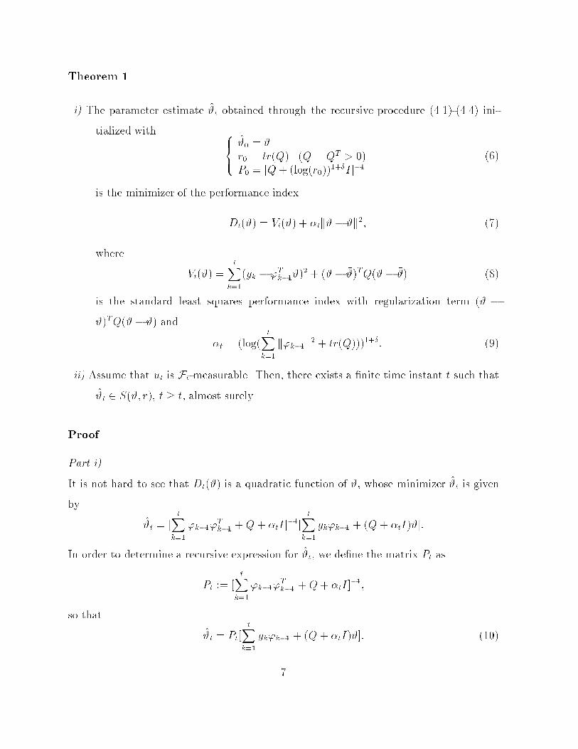
Theorem 1i) The parameter estimate #̂t obtained through the recursive procedure (4.1)-(4.4) ini-tialized with 8><>: #̂0 = �#r0 = tr(Q) (Q = QT > 0)P0 = [Q+ (log(r0))1+�I]�1 (6)is the minimizer of the performance indexDt(#) = Vt(#) + �tk#� �#k2; (7)where Vt(#) = tXk=1(yk � 'Tk�1#)2 + (#� �#)TQ(#� �#) (8)is the standard least squares performance index with regularization term (# ��#)TQ(#� �#) and �t = (log( tXk=1 k'k�1k2 + tr(Q)))1+�: (9)ii) Assume that ut is Ft-measurable. Then, there exists a �nite time instant �t such that#̂t 2 S(�#; r), t � �t, almost surely.Proof.Part i)It is not hard to see that Dt(#) is a quadratic function of #, whose minimizer #̂t is givenby #̂t = [ tXk=1'k�1'Tk�1 +Q+ �tI]�1[ tXk=1 yk'k�1 + (Q+ �tI)�#]:In order to determine a recursive expression for #̂t, we de�ne the matrix Pt asPt := [ tXk=1'k�1'Tk�1 +Q+ �tI]�1;so that #̂t = Pt[ tXk=1 yk'k�1 + (Q+ �tI)�#]: (10)7

It is easy to show that the term Ptk=1 yk'k�1 in the right-hand-side of this last equationcan be written astXk=1 yk'k�1 = yt't�1 + t�1Xk=1 yk'k�1 = yt't�1 + P�1t�1#̂t�1 � (Q+ �t�1I)�#:By substituting this last expression and the recursive expression for P�1t given byP�1t = P�1t�1 + 't�1'Tt�1 + (�t � �t�1)I (11)in equation (10), we conclude that #̂t can be determined as a function of the previousestimate #̂t�1 in the following way#̂t = Ptfyt't�1 + [P�1t � 't�1'Tt�1 � (�t � �t�1)I]#̂t�1 � (Q+ �t�1I)�#+ (Q+ �tI)�#g= #̂t�1 + Pt't�1(yt � 'Tt�1#̂t�1) + Pt(�t � �t�1)(�#� #̂t�1);which is just the recursive expression of #̂t in equation (4.2).The fact that �t given by (9) can be recursively computed through (4.3) and (4.4) withthe initialization r0 = tr(Q) given in (6) is a matter of a simple veri�cation.Finally, the fact that step 1 in the algorithm actually computes the inverse of matrix P�1tgiven in (11) is a simple application of the matrix inversion lemma and is left to the reader.This completes the proof of part i).Part ii)Denote by #̂LSt the minimizer of the least squares performance index Vt(#) and setQt = tXk=1'k�1'Tk�1 +Q: (12)It is then easy to show that #̂t = arg min#2Rn+m+1Dt(#) can be expressed as a function of #̂LStas follows #̂t = (Qt + �tI)�1Qt#̂LSt + �t(Qt + �tI)�1 �#:By subtracting �#, we get#̂t � �# = (Qt + �tI)�1Qt(#� � �#) + (Qt + �tI)�1Qt(#̂LSt � #�):8

Thus, the norm of #̂t � �# can be upper bounded as followsk#̂t � �#k � k#� � �#k+ k(Qt + �tI)�1Q 12t kkQ 12t (#̂LSt � #�)k: (13)We apply now Theorem 1 in reference [12] so as to upper bound the term kQ 12t (#̂LSt �#�)k.Since ut is assumed to be Ft-measurable, and also considering Assumption 1, by thistheorem we obtain the following upper bound:kQ 12t (#̂LSt � #�)k2 = O(log(tr(Qt))); a.s.. (14)The term k(Qt + �tI)�1Q 12t k can instead be handled as follows.Denote by f�1;t; : : : ; �n+m+1;tg the eigenvalues of the positive de�nite matrix Qt. SinceQt is symmetric and positive de�nite, there exists an orthonormal matrix Tt such thatQt = Tt diag(�1;t; : : : ; �n+m+1;t)T�1t and Q 12t = Tt diag �� 121;t; : : : ; � 12n+m+1;t�T�1t . Then,(Qt + �tI)�1Q 12t = Tt(T�1t (Qt + �tI)Tt)�1T�1t Q 12t TtT�1t= Tt diag 0B@ � 121;t�1;t + �t ; : : : ; � 12n+m+1;t�n+m+1;t + �t1CAT�1t :This implies that k(Qt + �tI)�1Q 12t k = maxi=1;:::;n+m+10B@ � 12i;t�i;t + �t1CA : (15)Consider now the function: f(x) = x 12x+ �t ; x � 0: Such a function has an absolutemaximum value 12�� 12t in x = �t. It then obviously follows from equation (15) thatk(Qt + �tI)�1Q 12t k � 12�� 12t : (16)Substituting the estimates (14) and (16) in equation (13), we obtaink#̂t � �#k � k#� � �#k+ h1 log(tr(Qt))�t ! 12 ;h1 being a suitable constant.Observe now that from equation (3) it follows that n2k � 2maxfk#�k2; 1g[ y2k + k'k�1k2 ].9

Taking into account that the autoregressive part of model (3) is not trivial (n > 0), this inturn implies that n2k � 2maxfk#�k2; 1g[ k'kk2 + k'k�1k2 ], from which it is easily shownthat tXk=1n2k � h2 t+1Xk=1 k'k�1k2;where h2 is a suitable constant. From Assumption 2 and de�nition (12) of Qt, we then getlimt!1 tr(Qt) =1:Since by de�nition (9) �t = (log(tr(Qt)))1+�, we then obtain that 8 � > 0 there exists atime instant � such that k#̂t � �#k � k#�� �#k+ �, 8 t � � . By Assumption 3, this impliesthat there exists a �nite time instant �t such that #̂t 2 S(�#; r), 8t � �t. This proves pointii). 2Part ii) in Theorem 1 shows that #̂t 2 S(�#; r), t � �t. This implies that the projectionoperation (4.5) is disconnected in the long run and, yet, the estimate lies inside the sphereS(�#; r). Since each model whose parameter belongs to S(�#; r) is controllable, from thisthe uniform controllability of the estimated model easily follows. In addition, thanks tothe fact that the projection is disconnected, in Theorem 2 below we shall be able to showthat the estimate �#t preserves closed-loop properties similar to those of the least squaresalgorithm. The properties of the estimate �#t stated in Theorem 2 are fundamental for asuccessful application of our identi�cation algorithm in adaptive control schemes suitablefor possibly nonminimum-phase systems. In particular, property i) is widely recognized ascrucial for a correct selection of the control law, see e.g. [5, 15, 14, 4]. Securing propertyii) is important for obtaining stability and performance results, see e.g. [8, 7]. We alsorefer the reader to [19] for a pole placement application where properties i) and ii) havebeen exploited.Recall that a standard measure of the controllability of model yt = 'Tt�1#+ nt is given bythe absolute value of the determinant of the Sylvester matrix given by10

Sylv(#) = 266666666666666664 1�a1 1�a2 �a1 . . .... �a2 . . . 1�as ... �a1�as �a2. . . ...�as| {z }s bdbd+1 . . .... . . . bdbs bd+1. . . ...bs377777777777777775| {z }s ; (17)where s = maxfn; d +mg (see e.g. [9]). In particular jdet(Sylv(#))j 6= 0 is equivalent tosay that the model whose parameter is # is controllable.Theorem 2 (Properties of the estimate �#t)i) There exists a constant c > 0 such that jdet(Sylv(�#t))j � c, 8 t, almost surely.ii) Assume that ut is Ft-measurable. Then, the identi�cation error satis�es the followingbound k#� � �#tk2 = O (log(Ptk=1 k'k�1k2))1+��min(Ptk=1 'k�1'Tk�1) ! almost surely. (18)Proof.Part i)Since the absolute value of the Sylvester matrix determinant is a continuous function ofthe system parameter # and it is strictly positive for any # 2 S(�#; r) (see Assumption 3),we can take c := min#2S( �#;r) jdet(Sylv(#))j> 0: (19)Point i) then immediately follows from the de�nition of �#t in equation (4.5).Part ii)Let us rewrite the performance index Dt(#) as a function of the least squares estimate11

#̂LSt = arg min#2Rn+m+1 Vt(#):Dt(#) = (#� #̂LSt )T [ tXk=1'k�1'Tk�1 +Q](#� #̂LSt ) + �tk#� �#k2 + Vt(#̂LSt ):From the de�nition of #̂t, it follows that(#̂t � #̂LSt )T [ tXk=1'k�1'Tk�1 +Q](#̂t � #̂LSt ) + �tk#̂t � �#k2� (#� � #̂LSt )T [ tXk=1'k�1'Tk�1 +Q](#�� #̂LSt ) + �tk#� � �#k2= O(�t); (20)almost surely, where the last equality is a consequence of the already cited Theorem 1 in[12] and of the boundedness of #�. Consider now the equation(#� � #̂t)T [ tXk=1'k�1'Tk�1 +Q](#� � #̂t) � 2((#� � #̂LSt )T [ tXk=1'k�1'Tk�1 +Q](#� � #̂LSt )+ (#̂LSt � #̂t)T [ tXk=1'k�1'Tk�1 +Q](#̂LSt � #̂t)) :Since in view of equation (20) both terms in the right-hand-side are almost surely O(�t),we get (#� � #̂t)T [ tXk=1'k�1'Tk�1 +Q](#�� #̂t) = O(�t)almost surely. From this,k#� � #̂tk2 = O �t�min(Ptk=1 'k�1'Tk�1 +Q)! almost surely.Since �#t = #̂t, 8t � �t (point ii) in Theorem 1) and also recalling de�nition (9) of �t, pointii) immediately follows. 2Remark 1 The convergence rate of the standard least squares estimate #̂LSt is given by(Theorem 1, [12]) k#� � #̂LSt k2 = O log(Ptk=1 k'k�1k2)�min(Ptk=1 'k�1'Tk�1)! :This is slightly better than the bound (18) due to the exponent 1 + � in this last bound.12

On the other hand, the least squares algorithm does not guarantee the estimated modelcontrollability. 24 ConclusionsIn the present contribution, we have introduced a new identi�cation algorithm securingthe estimated model controllability, which is widely recognized as a central problem inadaptive control. The proposed approach requires some a-priori knowledge on the regionto which the true parameter belongs, but, in contrast with the alternative stream ofmethods suitable for stochastic systems ([5, 13, 14, 4]), it has the main advantage to beeasily implementable. It is therefore suggested as an e�ective solution to the controllabilityproblem in all the situations in which the required a-priori knowledge is available.References[1] K. Arent, I.M.Y. Mareels, and J.W. Polderman. Adaptive control of linear systemsbased on approximate models. In Proc. 3rd Europ. Control Conf., pages 868{873,September 1995.[2] S. Bittanti and M. Campi. Least squares based self-tuning control systems. Identi�ca-tion, Adaptation, Learning. The science of learning models from data (S.Bittanti andG.Picci eds.). Springer-Verlag NATO ASI series - Computer and systems sciences,1996.[3] M.C. Campi. Adaptive control of non-minimumphase systems. Int. J. Adapt. Controland Signal Process., 9:137{149, 1995.[4] M.C. Campi. The problem of pole-zero cancellation in transfer function identi�cationand application to adaptive stabilization. Automatica, 32:849{857, 1996.[5] P. de Larminat. On the stabilizability condition in indirect adaptive control. Auto-matica, 20:793{795, 1984.[6] G.C. Goodwin and K.S. Sin. Adaptive control of nonminimum phase systems. IEEETrans. on Automatic Control, AC-26:478{483, 1981.13

[7] L. Guo. Self-convergence of weighted least-squares with applications to stochasticadaptive control. IEEE Trans. on Automatic Control, AC-41:79{89, 1996.[8] L. Guo and H.F. Chen. The Astr�om-Wittenmark self-tuning regulator revisedand ELS-based adaptive trackers. IEEE Trans. on Automatic Control, AC-36:802{812,1991.[9] T. Kailath. Linear Systems Theory. Englewood Cli�s, NJ: Prentice-Hall, 1980.[10] G. Kreisselmeier. A robust indirect adaptive control approach. Int. J. Contr., 43:161{175, 1986.[11] G. Kreisselmeier and M. Smith. Stable adaptive regulation of arbitrary nth orderplants. IEEE Trans. on Automatic Control, AC-31:299{305, 1986.[12] T.L. Lai and C.Z. Wei. Least squares estimates in stochastic regression models withapplications to identi�cation and control of dynamic systems. Ann. Statist., 10:154{166, 1982.[13] R. Lozano. Singularity-free adaptive pole placement without resorting to persistencyof excitation detailed analysis for �rst order systems. Automatica, 28:27{33, 1992.[14] R. Lozano and X.H. Zhao. Adaptive pole placement without excitation probingsignals. IEEE Trans. on Automatic Control, AC-39:47{58, 1994.[15] R.H. Middleton, G.C. Goodwin, D.J. Hill, and D.Q. Mayne. Design issues in adaptivecontrol. IEEE Trans. on Automatic Control, AC-33:50{58, 1988.[16] A.S. Morse and F.M. Pait. Mimo design models and internal regulators for cycliclyswitched parameter-adaptive control systems. IEEE Trans. on Automatic Control,AC-39:1172{1183, 1994.[17] K.A. Ossman and E.D. Kamen. Adaptive regulation of MIMO linear discrete-timesystems without requiring a persistent excitation. IEEE Trans. on Automatic Control,AC-32:397{404, 1987.[18] F.M. Pait and A.S. Morse. A cyclic switching strategy for parameter-adaptive control.IEEE Trans. on Automatic Control, AC-39:1172{1183, 1994.[19] M. Prandini and M.C. Campi. Adaptive pole placement by means of a simple, singu-larity free, identi�cation algorithm. To appear in Proc. 36th Conf. on Decision andControl, December 1997.[20] W. Ren. The self-tuning of stochastic adaptive pole placement controllers. In Proc.32nd Conf. on Decision and Control, pages 1581{86, December 1993.[21] C. Samson. An adaptive lq controller for non-minimum-phase systems. Int. J. Contr.,1:1{28, 1982. 14