Spatially-Adaptive Regularized Pel-Recursive MotionEstimation Based on the EM AlgorithmVania V. Estrelaa and Nikolas P. GalatsanosaaIllinois Institute of Technology, 3301 S. Dearborn St, Chicago, IL 60616, U.S.A.ABSTRACTPel-recursive motion estimation is a well-established approach. However, in the presence of noise, it becomes anill-posed problem that requires regulation. In the past, regularization for pel-recursive estimations was addressedin an ad-hoc manner. In this paper, a Bayesian estimation framework is used to to deal with this issue. Morespeci�cally, motion vectors and regularization parameters are estimated in an iterative fashion by means of theExpectation-Maximization (EM) algorithm and a Gaussian data model. The proposed algorithm utilizes the localimage properties to regularize the motion vector estimates following a spatially adaptive approach. Numericalexperiments are presented that demonstrate the merits of the proposed algorithm.Keywords: Motion estimatiom, EM algorithm, pel-recursive, maximum likelihood.1. INTRODUCTIONMotion estimation is vital in multimedia video processing applications. For example, in video coding, the estimatedmotion is used to reduce the transmission bandwidth. The evolution of an image sequence motion �eld can also helpother image processing tasks in multimedia applications such as analysis, recognition, tracking, restoration, collisionavoidance and segmentation of objects.In coding applications, a block-based approach is most oftenly used for interpolation of lost information betweenkey frames. The �xed rectangular partitioning of the image used by some block-based approaches often separatesvisually important image features. If the components of an important feature are assigned di�erent motion vectors,then the interpolated image will su�er from annoying artifacts. Pel-recursive schemes can theoretically overcomesome of the limitations associated with blocks by assigning a unique motion vector to each pixel. Intermediate framesare then constructed by resampling the image at locations determined by linear interpolation of the motion vectors.The pel-recursive approach can also manage motion with subpixel accuracy.We propose a Bayesian take on the pel-recursive motion paradigm, where its variables and an associated obser-vation noise are modelled as multivariate Gaussian processes. The parameters characterizing these processes can beestimated through the use of the maximum likelihood (ML) method. The corresponding ML estimate (MLE) is thevalue of the parameter that maximizes the ML function. This maximization can be very arduous when the systemis extremely nonlinear. The EM algorithm is an iterative numerical technique which can be used to determine themaximum likelihood estimate (MLE) of a set of parameters. This approach was formalized by Dempester et al,1and has been used in a variety of applications. In particular, it was previously used for motion estimation by Fan etal,2 with a di�erent formulation that deals with a�ne models of blocks of pixels. Each iteration is composed of anexpectation (E) step and a maximization (M) step. The E-step �nds the expected value of the unobserved variables,given the known values of the observed variables and the current estimate of the parameters. The M-step assumesthe values found in the previous step are correct and re-estimates the ML of the parameters.Further author information: (Send correspondence to N.P.G.)N.P.G.: E-mail: npg@argo.ece.iit.eduV.V.E.: E-mail: ve@argo.ece.iit.edu

2. PEL-RECURSIVE DISPLACEMENT ESTIMATION2.1. Problem CharacterizationThe displacement of each picture element in each frame forms the displacement vector �eld (DVF) and its estimationcan be done using at least two successive frames. The DVF is the 2-D motion resulting from the apparent motion ofthe image brightness (optical ow). A vector is assigned to each point in the image.Pel-recursive algorithms minimize the displaced frame di�erence function in a small causal area around theworking point assuming constant image intensity along the motion trajectory.A pixel is assumed to belong to a moving area if its intensity has changed between two consecutive frames.Consequently, our goal is to �nd the corresponding intensity value fk(r) of the k-th frame at location r = [x; y]T ,and d(r) = [dx; dy]T the corresponding (true) displacement vector at the working point r in the current frame. Thedisplaced frame di�erence (DFD) is de�ned by�(r;d(r)) = fk(r)� fk�1(r� d(r)) (1)and the perfect registration of frames will result in fk(r) = fk�1(r � d(r)). The DFD is a function of the intensitydi�erences and represents the error due to the nonlinear temporal prediction of the intensity �eld through thedisplacement vector. It is apparent from Eq. (1) that the relationship between the DVF and the intensity �eldis a nonlinear one. An estimate of d(r), is obtained by directly minimizing �(r;d(r)) or by determining a linearrelationship between the two. This is accomplished by using the Taylor series expansion of fk�1(r�d(r)) about thelocation (r� do(r)), where do(r) represents a prediction of d(r). This results in�(r; r� do(r)) = rTfk�1(r� bfdo(r))u(r) + e(r;do(r)) ; (2)where the displacement update vector u(r) = [ux; uy]T = d(r)�do(r), e(r;do(r)) represents the error resulting fromthe truncation of the higher order terms (linearization error) and r = [�=�x; �=�y]T represents the spatial gradientoperator. Applying Eq. (2) to all points in a neighborhood givesz = Gu+ n; (3)where the temporal gradients �(r; r� do(r)) have been stacked to form vector z, matrix G is obtained by stackingthe spatial gradient operators at each observation, and the error terms have formed the vector n.The observation vector z contains DFD information on all the pixels in a small pre-speci�ed neighborhood. Eq.(3) computes a new displacement estimate by using information contained in the neighborhood of the current pixel.It is mentioned here that if the neighborhood has N points, then z and �z are N � 1 vectors, G is an N � 2 matrixand u is a 2 � 1 vector. Since there is always noise present in the data, matrix G and vector z in Eq. (3) are inerror. Each row of matrixG has entries [gx; gy]T corresponding to a given pixel location inside a causal mask. Thespatial gradients of fk�1 are calculated by means of a bilinear interpolation scheme .32.2. Regularized Least-Squares (RLS) Method for Estimating the DVFThe pseudoinverse or least-squares (LS) estimate of the update vector is de�ned asuLS = (GTG)�1GTz (4)which is given by the minimizer of the functional J(u) = kz�Guk22. Since G may be very often ill-conditioned, thesolution given by Eq. (4) will be usually unacceptable due to the noise ampli�cation resulting from the calculationof the inverse matrix (GTG)�1. In other words, the data are erroneous or noisy. Therefore, one cannot expect anexact solution for Eq. (3), but rather an approximation according to some procedure.Previous works4{6 have shown that regularization improves the solutions to inverse problems. This techniqueameliorates the instability and non-uniqueness of inverse problems by introducing prior information using the regu-larization operator Q and the regularization parameter �. For linear observation models like the one in Eq. (3), theRLS solution results from the minimization ofJ�(u) = kz�Guk22 + �kQuk22 (5)

and is given by u(�) = (GTG+ �QTQ)�1GTz: (6)For the observation model in (3) the LMMSE (Wiener) solution is given by7uLMMSE = RuGT(GRuGT +Rn)�1z : (7)Using the matrix inversion lemma7 one can show that the RLS and the LMMSE solutions are identical when�QTQ = Rn(Ru)�1.It should be pointed out that uLMMSE requires the knowledge of th e covariance matrices of both the updateterm (Ru ) and the noise/linearization error term (Rn), respectively. The most common assumptions when dealingwith such problem is to consider that both vectors are zero mean valued, their components are uncorrelated amongeach other, with Ru = �2uI and Rn = �2nI where �2u and �2n are the variances of the components of the two vectors.Having those assumptions in mind, the RLS/LMMSE becomesu(�) = (GTG+ �I)�1GTz: (8)which corresponds to the estimate used in8 for pel-recursive DVF estimation with � = �2n=�2u. In our opinion thisestimate has �ve shortcomings: (a) no systematic approach was given to estimate the regularization parameter �,(b) the same value of the regularization parameter is used for the entire image which means that the estimate doesnot adapt to local variations, (c) LMMSE interpretation of the previous expression implies that the statistics ofthe DVF in both the x and the y directions are identical, (d) the term corresponding to the combined errors fromlinearization and noise is not always uncorrelated with the update term, and (e) the updates and noise/linearizationerrors at each pixel are not necessarily uncorrelated with each other.The e�ect of the regularization parameter and the regularization functional can be combined as follows: We makethe following assumption: �QTQ = � �1 00 �2 � = � : (9)3. EM ALGORITHM FORMULATIONLet us resume the motion model given by z = Gu+n. If z is the sample space from which the observations z 2 <mare drawn, and x is another sample space such that x 2 <n is an outcome from it, with m < n, then x is calledthe complete data and it is not observed directly. Instead, we have the observation z = z(x) which is a many-to-onemapping from x to z. Each value of z determines a subset of x. Therefore, x is available through z and it is notunique.We assume that the update vector u and the noise n are normally-distributed with mean zero and covariancematrices equal to �U and �N , respectively. If we consider u and n as being uncorrelated, then the pdf of z isfZ(z) = j2�(G�UGH + �N )j�12 exp��12 zH(G�UGH +�N )�1z� : (10)We take � = f�U ;�Ng as the parameter set to be estimated. The pdf is considered to be a continuous anddi�erentiable function of �. This dependency can be better captured by the notation fZ (z;�). Further we assumethat the additive noise is white, with covariance �N = �2N I, where I is an m �m identity matrix.The ML estimation of � is the value of �ML that maximizes the logarithm of the likelihood function fZ(z;�)which is given by �ML = argfmax� fZ(z;�)g = argfmax� log fZ(z;�)g : (11)Combining Eqs. (10) and (11), we conclude that the maximization of the log-likelihood function is equivalent tominimizing the function L(�) whereL(�) = log jG�UGH + �N )j+ zH (G�UGH +�N )�1z : (12)

The likelihood function L(�) from the previous equation is nonlinear with respect to �. Since analytical solutionsfor Eq. (12) are di�cult to be found or cannot be encountered, optimization techniques should be applied. The EMalgorithm arises as an alternative for estimating �.A successful application of the EM algorithm depends on the selection of an adequate set of parameters and datarepresentation. Let us choose x = (uT ;nT )T as the complete data where x 2 <(m+2)�1. Then, x will be normallydistributed with diagonal covariance matrix �X equal to�X = � �U 00 �N � ; with inverse ��1X = � ��1U 00 ��1N � : (13)Eq. (3) can be re-written as z = [G; I]� un � = Hx : (14)4. DERIVATION OF THE EM ALGORITHMThe foundation of the EM algorithm is the maximization of the expectation of log fX (x;�) given the incompleteobserved data z and the current estimate of the parameter set �. fX (x;�) is the pdf of the complete data and isgiven by fX (x;�) = j2��X j�12 exp��12 xH (�X�X )�1x� : (15)Taking the logarithm of both sides of Eq. (15) leads tolog fX (x;�) = �12 log j2��X j = K � 12 �log j�X j � xH��1X x (16)where � = �X and K is a constant independent of �. The E-step requiresQ(�;�(p)) = E[log fX(x;�)jz;�(p)] : (17)where �(p) = f�(p)U ;�(p)N g is the estimate of the parameter set � = f�U ;�Ng at the p-th iteration. The M-stepmaximizes Q(�;�(p)): �(p+1) = argfmax� Q(�;�(p))g : (18)The EM algorithm converges to a stationary point, if Q(�;�(p)) is continuous in � and �(p). In view of the fact thatEq. (17) is monotonically nondecreasing, Eq. (18) will converge to a maximum. However, for likelihood functionswith multiple maxima, the procedure may converge to a local minimum due to the starting point �(0).Now, let us resume the E-step as stated in Eq. (17)Q(�;�(p)) = K � 12 nE[log j�X jjz;�(p)] +E[xH��1X xjz;�(p)]o = K � 12 nlog j�X j+ tr(��1X C(p)Xjz)o : (19)where tr(:) stands for the trace of a matrix and C(p)Xjz is the covariance matrix of the event fXjzg at iteration p whichtakes the form C(p)Xjz = E[XXH jz;�(p)] = �(p)Xjz + �(p)Xjz�(p)HXjz = E[Xjz;�(p)] : (20)Maximizing Eq. (19) is tantamount to minimizing F (�;�(p)) = log j�X j+ tr(��1X C(p)Xjz). Combining the past twostatements, allows us to re-state the E-step in terms of the statistics of the complete data X and the event fXjzg:F (�;�(p)) = log j�X j+ tr(��1X �(p)Xjz + �(p)HXjz ��1X �(p)Xjz ; (21)where the conditional pdf p(xjz) is also normal with mean�Xjz = E(Xjz) = E(X) + �Xz��1zz (z� E(z)) = �Xz��1zz z : (22)In order to rewrite Eq. (22) in terms of the parameter set � = f�U ;�Ng, we need the following equations:�Xz = E(XzH ) = E(XXHHH ) = �XXHH ; (23)

�zX = E(zXH) = E(HXXH ) = H�XX , and (24)�zz = E(zzH) = E(HXXHHH ) = H�XXHH : (25)Inserting Eqs. (23)-(25) in Eq. (22) we get�Xjz = �XXHH (H�XXHH )�1z = � �UGH(G�UGH +�N )�1z�N (G�UGH + �N )�1z � , and (26)�(p)Xjz = " �(p)U GH(G�(p)U GH +�(p)N )�1z�(p)N (G�(p)U GH + �(p)N )�1z # : (27)From Eq. (27) we can obtain �(p)HXjz . Now, we need �(p)Xjz in order to fully characterize p(Xjz):�(p)Xjz = �(p)XX � �(p)Xz�(p)z �(p)zX = �(p)XX ��(p)X HH (H�(p)X HH)�1H�(p)X : (28)Eq. (28) can be expressed as �(p)Xjz = " �(p)U ��(p)U GH(G�(p)U GH + �(p)N )�1G�(p)U�(p)N ��(p)N (G�(p)U GH + �(p)N )�1�(p)N # = " �(p)Ujz�(p)Njz #.Finally, the E-step as enunciated in Eq. (21) can be re-written in terms of the parameter set � by means of therelationships developed in terms of the complete data X and the pdf p(xjz;�(p)):F (�;�(p)) = log j�U j+ log j�N j+ tr(��1U �(p)Ujz) + tr(��1N �(p)Njz) + �(p)HUjz ��1U �(p)Ujz + �(p)HNjz ��1N �(p)Njz : (29)Now, recalling that our ultimate goal is to estimate the update vector u, we shall examine the previous expressions.A good estimate for u is �(p)HUjz which corresponds to its mean value at iteration p, given the observation z. Hence,it is obvious from Equations (27), (27), and (29). that this estimate is a subproduct of the estimation of �.4.1. Simpli�cations and AlgorithmWe will consider �U = � �21 00 �22 � ; and �N = �2N 26664 1 0 : : : 00 1 : : : 0... ... . . . ...0 0 : : : 1 37775 = �2NIm :The above notation results in � = f�21; �22; �2Ng where �N is an m � m matrix with m being the size of theneighborhood. F (�;�(p)) can be further developed as a function of �U and �U asF (�;�(p)) = log j�U j + log j�N j+ trn��1N [�(p)N ��(p)N (G�(p)U GH + �(p)N )�1�(p)N ]o+ tr���1U ��(p)U � �(p)U GH �G�(p)U GH + �(p)N ��1G�(p)U ��+ ��(p)U GH �G�(p)U GH + �(p)N ��1 z�H ��1U ��(p)U GH �G�(p)U GH + �(p)N ��1 z�+ n�(p)N (G�(p)U GH + �(p)N )�1zoH ��1N n�(p)N (G�(p)U GH + �(p)N )�1zo : (30)Eq. (30) can be rewritten asF (�;�(p)) = log�det � �21 00 �22 �� + log j�2NImj+ tr(� �21 00 �22 � " a(p)11 a(p)12a(p)21 a(p)22 #)+ tr� 1�2N ImB(p)� + cT � �21 00 �22 � c+ dT 1�2N d (31)

where A(p) = ��(p)U ��(p)U GH �G�(p)U GH +�(p)N ��1G�(p)U � = " a(p)11 a(p)12a(p)21 a(p)22 # ; (32)B(p) = �(p)N � �(p)N (G�(p)U GH +�(p)N )�1�(p)N = 266664 b(p)11 b(p)12 : : : b(p)1mb(p)21 b(p)22 : : : b(p)2m... ... . . . ...b(p)m1 b(p)m2 : : : b(p)mm 377775 ; (33)c(p) = " c(p)1c(p)2 # = ��(p)U GH �G�(p)U GH +�(p)N ��1 z� ; and (34)d(p) = " d(p)1d(p)m # = n�(p)N (G�(p)U GH +�(p)N )�1zo : (35)By evaluating the determinants and traces from the previous equation, we getF (�;�(p)) = log(�21) + log(�22) + log(m) + log(�2N ) + (a11 + c21)�21 + (a22 + c22)�22+ (b11 + : : :+ bmm + d21 + : : :+ d2m)�2N : (36)Di�erentiating F (�;�(p)) with respect to �2N and making it equal to zero yields�2(p+1)N = b(p)11 + : : :+ b(p)mm + d2(p)1 + : : :+ d2(p)m : (37)Applying similar procedure for �21 and �22, gives�2(p+1)1 = a(p)11 + c2(p)1 , and (38)�2(p+1)2 = a(p)22 + c2(p)2 : (39)ALGORITHM:Assume a pixel at location r with intensity fk(r) and belonging to a neighborhood i ; i = 1; : : : ; N .Step1. Inicialize � for p = 0, that is, �2(0)N , �2(0)1 , and �2(0)2 .Step 2. Compute the E-step from Eqs. (32)-(35), that is, as a function of the current estimates for �).Step 3. Perform the M-step using the new parameter estimates from Eqs. (37)-(39).Step 4. If j�(p+1) ��(p)j < �, then validate the estimation. Otherwise, increment p and go to step 2.This algorithm will stop after a number P of updatings, if there is no convergence. In general, it converges invery few iterations. 5. EXPERIMENTSThe pel-recursive problem per si poses heavy computacional burden. First, since we have to perform a minimizationper pixel, the same initial estimate for � would not work well for the entire image (for explanations, see9). Ourapproach to circunvent this problem was to use a �nite set of initial estimates. The adaptivity we introduced istwo-fold. First, a separate set of parameters � is found for each pixel. Second, the region around each pixel that isassumed to have the same motion is changed, in order to account for motion boundaries in the DVF. We test the setof nine neighborhoods shown in Fig. (1). The cross indicates the pixel whose motion is being currently estimated.Circles represent its eight neighbors which are regarded as having the same motion according to Eq. (3). The best

neighborhood is the one which gives the smallest estimated image motion variance as de�ned by.10 This con�dencemeasure is estimated from the noise variance in the measurements of the residual error e = z �Gu = �z. Underthe assumptions that our model is correct, the estimated variance �2max of the motion vectors equals:�2max = eTeM�min (40)where �min is the minimum eigenvalue of (GTG)�1. In this section, we present experimental results that illustratethe e�ectiveness of the proposed adaptive EM-based approach and compare it with the LMMSE/MAP �lter fromEq. (8). This approach relies on the fact that the system of constraint equations is obtained assuming the motion�eld varies slowly across the image. The smoothness constraint is enforced by considering the optical ow constantover the neighborhood from which the system is taken. Hence, we have a way of picking up a better conditionedsystem. This is helpful specially at regions where the ow changes abruptly such as the border between two objectswith di�erent motion. There will be always a neighborhood that will group pixels with similar motion. It should bepointed out that most of the masks represent a guess about the direction in which the ow must be analyzed. Thechoice of direction a�ects the overall error in the optical ow estimate.Mask 1

O

O

O

X

O

O

O

O

O

Mask 2

O O O

O O O

O X O

Mask 3

X

O

O

O

O

O

O

O

O

Mask 4

X

O

O

O

O

O

O

O

O

Mask 5

O

O

O

X

O

O

O

O

O

Mask 6

O

O O

O

O

OO

OOX

Mask 7

O

OO

O

O

O

OO

X

Mask 8

O

OO

O

O

O

OO

X

Mask 9

O

O O

O

O

O O

OXFigure 1. Set of multiple masks used to improve the algorithm.In this section, we present several experimental results that illustrate the e�ectiveness of the EM algorithm andcompare it with the Wiener �lter. As before, the algorithms were tested on a synthetic sequence and the two realvideo sequences "Foreman" and "Mother and Daughter". The sequences are 144�176, 8-bit (QCIF). In this sequence,there is a moving object in a moving background. It was created using the following auto-regressive model:f(m;n) = 0:333[f(m;n� 1) + f(m � 1; n) + f(m � 1; n� 1)] + ni(m;n) (41)For the background, n1 is a Gaussian random variable with mean �1 = 50 and variance �21 = 49. The rectangle wasgenerated with �2 = 100 and variance �22 = 25. We developed a program based on the EM technique and using themultimask approach described earlier. Results from the EM algorithm are compared to the ones obtained with theWiener �lter Eq. ( 8).5.1. Experiment 1Here, some results for the "Synthetic" sequence are presented. Table 1 shows the values for the mean-squarederror(MSE), bias, IMC(dB) and DFD2 for the estimated optical ow using the Wiener �lter and EM algorithmfor frames 1 and 2 of the noiseless "Synthetic" sequence. The actual motion from two consecutive frames of thesynthetic sequence is known, therefore we can evaluate the MSE and bias in the horizontal and vertical directions.These metrics are given by: MSEi = 1MN Xr2S(di(r)� di(r))2 (42)

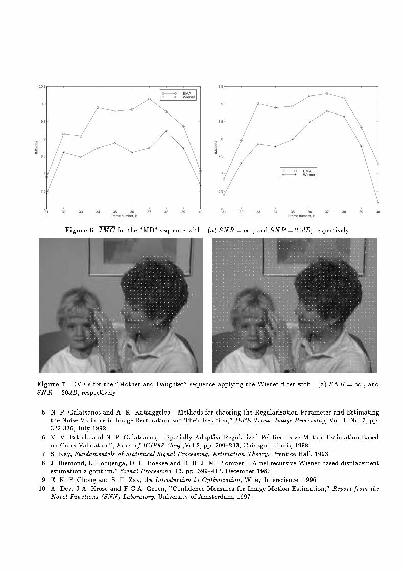
where S is the entire frame and i = x; y, andbiasi = 1MN Xr2S(di(r)� di(r)) (43)Other two helpful metrics are the average mean-squared displaced frame di�erence (DFD2) de�ned asDFD2 = PKk=2Prk (fk(r)� fk�1(r� d(r)))2(Numb:ofP ixels)(Numb:offrames) (44)and the average improvement in motion compensation (IMC) in dB given byIMC = 10 log10 PKk=2Prk (fk(r)� fk�1(r))2PKk=2Prk(fk(r)� fk�1(r� d(r)))2 (45)Table 2 shows the values for the MSE, bias, IMC(dB) and DFD2 for the estimated optical ow using the WienerTable 1. Comparison between the Wiener �lter and the EM implementation. Synthetic sequence, SNR =1Metric Wiener EMMSEx 0.1548 0.1364MSEy 0.0740 0.0581biasx 0.0610 0.0566biasy -0.0294 -0.0180IMC(dB) 19.46 17.18DFD2 4.16 10.02�lter and the EM algorithm with multiple masks for the noisy frames 1 and 2 of the "Synthetic" sequence withSNR = 20dB. The estimated DVF's obtained with the Wiener �lter and the EM algorithm for the noiseless andTable 2. Comparison between the Wiener �lter and the EM algorithm. Frames 1 and 2 of the "Synthetic" sequence,SNR = 20dB Metric Wiener EMMSEx 0.2563 0.2332MSEy 0.1273 0.1247biasx 0.0908 0.0880biasy -0.0560 -0.0507IMC(dB) 14.74 15.30DFD2 12.24 11.31noisy cases of the "Synthetic" sequence are shown in Fig. 2 and Fig. 3. The motion-compensated frames correspondingto those DVF's are presented in Fig. 4 and Fig. 5.5.2. Experiment 2This experiment uses the "Mother and Daughter" sequence which contains small amount of motion. Fig. 6 presentsthe values of the IMC(dB) from frames 31 to 40 of the "Mother and Daughter" sequence for the noiseless and noisy(SNR = 20dB) cases, respectively, for both algorithms investigated. The EM technique provides, on the average,1.5 dB higher IMC than the LMMSE algorithm. Their qualitative performance can be observed in Fig. 7 -Fig. 10.5.3. Experiment 3The objective of this experiment is to test the proposed algorithms with an image sequence containing a more di�culttype of motion. Figs. 11 demonstrate results obtained for frames 11-20 of the "Foreman" sequence. Figs. 12 - 15demonstrate qualitative results obtained for frames 11-20 of this sequence.

Figure 2. DVF for the Wiener �lter with (a) SNR =1 , and SNR = 20dB, respectively.Figure 3. DVF for the EM algorithm with (a) SNR =1 , and SNR = 20dB, respectively.6. CONCLUSIONSThe present work employes a framework that takes into consideration the existence of noise and errors in a LMMSEestimate systematicly. First, we estimate the regularization parameters on a pixel-by-pixel basis as a maximumlikelihood (ML) estimation problem. Second, we use a systematic approach to select the optimal region of supportfor our model on a pixel-by-pixel basis. Finally, we developed a computationally e�cient scheme to implement thissolution.The non-convexity of the likelihood function makes its direct optimization very demanding. As an alternative,we use the Expectation-Maximization EM) technique, which determines the ML estimate (MLE) with simultaneousestimation of the regularization parameters and the motion vectors. No knowledge of the statistics of the errorscorrupting the data is required. The resulting closed-form expressions ensue a fast implementation of the MLE.Numerous experiments done with di�erent signal-to-noise ratios (SNRs) demonstrate the e�ectiveness of the EMtechnique when compared to the Wiener �lter.The EM algorithm performed better than the LMMSE for both noiseless and noisy images in the MSE, the IMCand the DFD squared senses.

Figure 4. Motion compensation error for the Wiener �lter with (a) SNR =1 , and SNR = 20dB, respectively.Figure 5. Motion compensation error for the EM algorithm with (a) SNR =1 , and SNR = 20dB, respectively.In practical terms, the EM algorithm implementation showed the expected theoretical improvements: rapidconvergence, no need to compute optmizations, and robustness. The proposed Our strategy of using several masksand picking up an estimate based on the variance of the motion estimates as well as several initial estimates for theregularization parameter made the technique more robust than using it with just one mask and one initial estimate.REFERENCES1. A. P. Dempster, N.M. Laird and D. B. Rubbin, \Maximum Likelihood From Incomplete Data via the EMAlgorithm," Ann. Roy. Statist. Soc., Vol. 39, pp. 1-38, Dec. 1977.2. C.M. Fan, N.M. Namazi and P.B. Pena�el, "A New Image Motion Estimation Algorithm Based on the EMTechnique," IEEE Transactions on Pattern Analysis and Machine Intelligence, Vol. 18, No. 3, pp. 348-352,1996.3. S. N. Efstratiatis, Adaptive Constrained Recursive Motion Field and Image Sequence Estimation, Ph.D. Thesis,Dept. of Electrical and Computer Engineering, Evanston, Illinois, 1991.4. A. Tikhonov and V. Arsenin, Solution of Ill-Posed Problems, John Wiley and Sons, 1977.

31 32 33 34 35 36 37 38 39 407

7.5

8

8.5

9

9.5

10

10.5

Frame number, k

IMC

(dB

)

EMA Wiener

31 32 33 34 35 36 37 38 39 406

6.5

7

7.5

8

8.5

9

9.5

Frame number, kIM

C(d

B)

EMA WienerFigure 6. IMC for the "MD" sequence with (a) SNR =1 , and SNR = 20dB, respectively.

Figure 7. DVF's for the "Mother and Daughter" sequence applying the Wiener �lter with (a) SNR = 1 , andSNR = 20dB, respectively.5. N. P. Galatsanos and A. K. Katsaggelos, \Methods for choosing the Regularization Parameter and Estimatingthe Noise Variance in Image Restoration and Their Relation," IEEE Trans. Image Processing, Vol. 1, No. 3, pp.322-336, July 1992.6. V. V. Estrela and N. P. Galatsanos, \ Spatially-Adaptive Regularized Pel-Recursive Motion Estimation Basedon Cross-Validation", Proc. of ICIP98 Conf.,Vol.2, pp. 200{203, Chicago, Illinois, 1998.7. S. Kay, Fundamentals of Statistical Signal Processing, Estimation Theory, Prentice Hall, 1993.8. J. Biemond, L. Looijenga, D. E. Boekee and R. H. J. M. Plompen, \A pel-recursive Wiener-based displacementestimation algorithm," Signal Processing, 13, pp. 399{412, December 1987.9. E. K. P. Chong and S. H. Zak, An Introduction to Optimization, Wiley-Interscience, 1996.10. A. Dev, J.A. Krose and F.C.A. Groen, "Con�dence Measures for Image Motion Estimation," Report from theNovel Functions (SNN) Laboratory, University of Amsterdam, 1997.

Figure 8. DVF's for the EM algorithm applied to frames 32 and 33 of the "Mother and Daughter" sequence with(a) SNR =1 , and SNR = 20dB, respectively.

Figure 9. Motion compensation error for the "Mother and Daughter" sequence applying the Wiener �lter with (a)SNR =1 , and SNR = 20dB, respectively.

Figure 10. Motion compensation error for the EM algorithm applied to frames 32 and 33 of the "Mother andDaughter" sequence with (a) SNR =1 , and SNR = 20dB, respectively.11 12 13 14 15 16 17 18 19 20

8.5

9

9.5

10

10.5

11

11.5

12

12.5

Frame number, k

IMC

(dB

)

EMA Wiener

11 12 13 14 15 16 17 18 19 207.5

8

8.5

9

9.5

10

10.5

11

Frame number, k

IMC

(dB

)

EMA Wiener

Figure 11. IMC for the "Foreman" sequence with (a) SNR =1 , and SNR = 20dB, respectively.

Figure 12. DVF's for the "Foreman" sequence applying the Wiener �lter with (a) SNR =1 , and SNR = 20dB,respectively.

Figure 13. DVF's for the EM algorithmapplied to frames 32 and 33 of the "Foreman" sequence with (a) SNR =1, and SNR = 20dB, respectively.

Figure 14. Motion compensation error for the "Foreman" sequence applying the Wiener �lter with (a) SNR =1, and SNR = 20dB, respectively.

Figure 15. Motion compensation error for the EM algorithm applied to frames 32 and 33 of the "Foreman" sequencewith (a) SNR =1 , and SNR = 20dB, respectively.