
SIGN SINGULARITY AND FLARES IN SOLAR ACTIVE REGION NOAA 11158
Upload
khangminh22Category
view
0download
0
Bachelor’s degree thesis
Workspace and singularity
determination of a 7-DoF
wrist-partitioned serial manipulator
towards graffiti painting
Marc Esquerra Corominas
Advisors:
Frank Dellaert (Georgia Institute of Technology)
Carme Torras Genıs (UPC)
In partial fulfillment of the requirements for the:
Bachelor’s degree in Mathematics
Bachelor’s degree in Industrial Technology Engineering
May 2020

i
Abstract
Workspace and singularity determination of a 7-DoF
wrist-partitioned serial manipulator towards graffiti
paintingby Marc Esquerra Corominas
Robots are overtaking every day more tasks in the industry. A lot of them are even designed for perform-
ing household chores. In general, robots are designed to facilitate the day-to-day of human beings. But
when it comes to artistic tasks, it is less usual to see robots performing them. We pretend to stay out
of the crowd by using a robot to paint a graffiti. The motivation to achieve this task converges into the
statement of two questions: ”What is the workspace of a robot, when the orientation of its end-effector
is fixed?” and ”For a given plane, what is the largest singularity free surface on it?”.
This thesis proposes a method for the computation of the position singularities of a wrist-partitioned se-
rial manipulator for a given plane. The method is obtained from the combination of a position singularity
determination method, which is based on the decoupling technique of a wrist-partitioned manipulator,
and a branch-and-prune algorithm for the resolution of systems of equations.
The workspace of a 7-DoF serial manipulator is obtained by a forward kinematics approach. A method-
ology to obtain the constant orientation workspace of a serial manipulator is presented and applied to
get approximations for some specific orientations.
It is shown how singularities can be analyzed by decoupling them into position singularities and ori-
entation singularities. The proposed method formulates and solves the equation that determines the
position singularities. In the case of the orientation singularities, it is shown that they can be avoided
without losing a significant amount of the workspace’s volume, from the point of view of the position.
Keywords: Workspace, singularity, end-effector, wrist-partitioned manipulator.
Mathematics Subject Classification American Mathematical Society code: [70b10].

ii
Resumen
Determinacion del volumen de trabajo y las
singularidades de un manipulador serial redundante
de 7 grados de libertad con muneca esferica
orientadas al grafitipor Marc Esquerra Corominas
Los robots estan siendo utilizados, cada vez mas, en la realizacion de tareas en la industria. Muchos
de ellos tambien son disenados pensados para realizar las tareas del hogar. En general, los robots son
disenados para facilitar el dıa a dıa de los seres humanos. Pero cuando se trata de obras artısticas, es
menos comun encontrarse a robots realizandolas. Nosotros pretendemos salirnos de lo comun mediante
el uso de un robot para pintar un grafiti. La motivacion por lograrlo converge en la formulacion de dos
preguntas: ”¿Cual es el volumen de trabajo de un robot, cuando la orientacion de su efector final esta
fijada?” y ”Dado un plano arbitrario, ¿cual es la mayor area de trabajo libre de singularidades en este?”
Esta tesis propone un metodo para la obtencion de las singularidades de posicion en un plano cualquiera
de un manipulador serial con una muneca esferica. El metodo ha sido obtenido mediante la combinacion
de un metodo de determinacion de singularidades de posicion, el cual esta basado en una tecnica para el
decoplado de manipuladores que presentan una muneca esferica, y un algoritmo branch-and-prune para
la resolucion de sistemas de ecuaciones.
Se ha obtenido el volumen de trabajo de un manipulador serial de 7 grados de libertad a traves de
un enfoque de cinematica directa. Se presenta la metodologıa para obtener el volumen de trabajo del
manipulador serial cuando su efector final tiene una orientacion constante y se aplica para obtener aprox-
imaciones para el caso de ciertas orientaciones.
Se muestra como las singularidades pueden ser analizadas a traves de separarlas en singularidades de
posicion y de orientacion. El metodo propuesto formula y resuelve las ecuaciones que determinan las sin-
gularidades de posicion. En cuanto a las singularidades de orientacion, se muestra que pueden ser evitadas
sin perder una cantidad significante de volumen de trabajo, desde el punto de vista de la posicion.
Palabras clave: Volumen de trabajo, singularidad, efector final, manipulador con muneca esferica.
Codigo de clasificacion de la American Mathematical Society : [70b10].

iii
Resum
Determinacio del volum de treball i les singularitats
d’un manipulador serial redundant de 7 graus de
llibertat amb canell esferic orientades al grafitiper Marc Esquerra Corominas
Els robots estan sent utilitzats, cada cop mes, en la realitzacio de tasques en la industria. Molts d’ells
tambe son dissenyats pensats per a realitzar les tasques de la llar. En general, els robots son dissenyats
per a facilitar el dia a dia del essers humans. Pero quan es tracta d’obres artıstiques, es menys comu
trobar-se robots realitzant-les. Nosaltres pretenem sortir de la norma mitjancant l’us d’un robot per a
pintar un grafiti. La motivacio per a aconseguir-ho convergeix en la formulacio de dues preguntes: ”Quin
es el volum de treball d’un robot, quan l’orientacio del seu efector final esta fixada?” i ”Donat un pla
arbitrari, quina es la major area de treball lliure de singularitats en aquest?”
Aquesta tesi proposa un metode per a l’obtencio de les singularitats de posicio en un pla qualsevol
d’un manipulador serial amb un canell esferic. El metode s’ha obtingut mitjancant la combinacio d’un
metode de determinacio de singularitats de posicio, el qual esta basat en una tecnica per al decoplat
de manipuladors que presenten un canell esferic, i un algorisme branch-and-prune per a la resolucio de
sistemes d’equacions.
S’ha obtingut el volum de treball d’un manipulador serial de 7 graus de llibertat a traves d’un enfocament
de cinematica directa. Es presenta una metodologia per a obtenir el volum de treball del manipulador
serial quan el seu efector final te l’orientacio constant i s’aplica per a obtenir aproximacions per al cas de
certes orientacions.
Es mostra com les singularitats poden ser analitades a traves de separar-les en singularitats de posicio i
d’orientacio. el metode proposat formula i resol les equacions que determinen les singularitats de posicio.
Pel que fa a les singularitats d’orientacio, es mostra que poden ser evitades sense perdre una quantitat
significant de volum de treball, des del punt de vista de la posicio.
Paraules clau: Volum de treball, singularitas, efector final, manipulador amb canell esferic.
Codi de classificacio de la American Mathematical Society : [70b10].

iv
Acknowledgement
First of all, special thanks to Dr. Frank Dellaert for supervising my project and giving me the huge
opportunity of working in his lab at the Georgia Institute of Technology. Thanks to Dr. Carme Torras
Genıs for being my supervisor from my home institution (UPC) and helping me to finish my thesis. I
would also like to thank Gerry Chen guiding me during all my stay in Atlanta and ensuring the success
of my project. Thanks to Suyoung Park and Yoonwoo Kim for working with me during the past months
and sharing all their results.
Thanks to all the CFIS members for organizing my exchange program. My gratitude goes specially
to Toni Pascual and Loli Hernandez for closely following my personal status and helping me with all the
required documentation. Thanks to Fundacio Privada CELLEX for the financial support during this
experience.
Last but not least, I would like to thank my beloved ones for being always supportive. In particu-
lar, thanks to my US and Czech family; Albert, Eric, Jordi, Oscar and Erik, for the good lived moments.
Thanks to Alba for the laughs and the great company. Thanks to Vera for all the long talks and giving
me a reason to be happy every day. Thank you to my parents for giving me a great education that has
taken me to have amazing opportunities like this one.

Contents
1 Introduction 1
2 Basic concepts 3
2.1 Configuration space and degrees of freedom . . . . . . . . . . . . . . . . . . . . . . . . . . 3
2.2 Three-dimensional Geometry . . . . . . . . . . . . . . . . . . . . . . . . . . . . . . . . . . 3
2.2.1 Rotation matrices . . . . . . . . . . . . . . . . . . . . . . . . . . . . . . . . . . . . 4
2.3 Homogeneous transformation matrices . . . . . . . . . . . . . . . . . . . . . . . . . . . . . 4
2.4 Spatial twists . . . . . . . . . . . . . . . . . . . . . . . . . . . . . . . . . . . . . . . . . . . 6
2.5 Serial link manipulators . . . . . . . . . . . . . . . . . . . . . . . . . . . . . . . . . . . . . 7
2.6 Forward Kinematics . . . . . . . . . . . . . . . . . . . . . . . . . . . . . . . . . . . . . . . 8
2.6.1 Product of Exponentials Formula . . . . . . . . . . . . . . . . . . . . . . . . . . . . 8
2.7 The Jacobian manipulator . . . . . . . . . . . . . . . . . . . . . . . . . . . . . . . . . . . . 10
2.8 Singularities . . . . . . . . . . . . . . . . . . . . . . . . . . . . . . . . . . . . . . . . . . . . 11
2.9 Inverse Kinematics . . . . . . . . . . . . . . . . . . . . . . . . . . . . . . . . . . . . . . . . 12
2.10 Redundant and wrist-partitioned manipulators . . . . . . . . . . . . . . . . . . . . . . . . 13
2.10.1 Redundant manipulators . . . . . . . . . . . . . . . . . . . . . . . . . . . . . . . . . 13
2.10.2 Wrist-partitioned manipulators . . . . . . . . . . . . . . . . . . . . . . . . . . . . . 13
3 Workspace 14
3.1 Definition and categories . . . . . . . . . . . . . . . . . . . . . . . . . . . . . . . . . . . . . 14
3.2 Workspace determination . . . . . . . . . . . . . . . . . . . . . . . . . . . . . . . . . . . . 15
3.2.1 Workspace determination methods . . . . . . . . . . . . . . . . . . . . . . . . . . . 16
3.3 Own approach and results . . . . . . . . . . . . . . . . . . . . . . . . . . . . . . . . . . . . 23
3.3.1 Forward kinematics model . . . . . . . . . . . . . . . . . . . . . . . . . . . . . . . . 23
3.3.2 Sampling . . . . . . . . . . . . . . . . . . . . . . . . . . . . . . . . . . . . . . . . . 26
3.3.3 Reachable workspace . . . . . . . . . . . . . . . . . . . . . . . . . . . . . . . . . . . 26
3.3.4 Constant orientation workspace . . . . . . . . . . . . . . . . . . . . . . . . . . . . . 27
4 Singularity analysis and visualization 34
4.1 Related work . . . . . . . . . . . . . . . . . . . . . . . . . . . . . . . . . . . . . . . . . . . 34
v

CONTENTS vi
4.2 Directly accessible workspace . . . . . . . . . . . . . . . . . . . . . . . . . . . . . . . . . . 35
4.3 Decoupling of wrist-partitioned manipulators . . . . . . . . . . . . . . . . . . . . . . . . . 37
4.3.1 Position singularities . . . . . . . . . . . . . . . . . . . . . . . . . . . . . . . . . . . 39
4.3.2 Orientation singularities . . . . . . . . . . . . . . . . . . . . . . . . . . . . . . . . . 41
4.4 Visualization . . . . . . . . . . . . . . . . . . . . . . . . . . . . . . . . . . . . . . . . . . . 41
4.5 Own approach and results . . . . . . . . . . . . . . . . . . . . . . . . . . . . . . . . . . . . 44
4.5.1 Position singularities . . . . . . . . . . . . . . . . . . . . . . . . . . . . . . . . . . . 44
4.5.2 Orientation singularities . . . . . . . . . . . . . . . . . . . . . . . . . . . . . . . . . 47
5 Conclusions 50
6 Future work 51
6.1 Test results on the physical robot . . . . . . . . . . . . . . . . . . . . . . . . . . . . . . . . 51
6.2 Mobile manipulation . . . . . . . . . . . . . . . . . . . . . . . . . . . . . . . . . . . . . . . 51
6.3 Crossable and non-crossable singularity sets . . . . . . . . . . . . . . . . . . . . . . . . . . 51
6.4 Spray can manipulation . . . . . . . . . . . . . . . . . . . . . . . . . . . . . . . . . . . . . 52
Appendices 53
A The CuikSuite 54
A.1 Description and examples of .world files . . . . . . . . . . . . . . . . . . . . . . . . . . . . 54
A.2 Singularity determination commands . . . . . . . . . . . . . . . . . . . . . . . . . . . . . . 58

List of Figures
2.1 Mathematical description of position and orientation Source: [23]. . . . . . . . . . . . . . 5
2.2 Illustration of the process used to obtain the Product of Exponentials Formula. Source: [23] 9
2.3 3R planar manipulator at a singular configuration. Only vertical movement for the end-
effector is possible. . . . . . . . . . . . . . . . . . . . . . . . . . . . . . . . . . . . . . . . . 11
2.4 Illustration of reachability of different desired positions by a 2R planar manipulator. The
red position can’t be achieved (no inverse kinematics solution), the blue position can be
reached just by the configuration where the manipulator is fully stretched out (black links)
and the green position presents two different inverse kinematics solutions (gray links). . . 12
3.1 Reachable (green) and dexterous (blue) workspace for a planar manipulator with two
revolute joints. Source: [22]. . . . . . . . . . . . . . . . . . . . . . . . . . . . . . . . . . . . 15
3.2 Constant orientation workspace for two different orientations (blue and green) and total
orientation workspace (violet) for a planar manipulator with two revolute joints. Source:
[22]. . . . . . . . . . . . . . . . . . . . . . . . . . . . . . . . . . . . . . . . . . . . . . . . . 15
3.3 Orientation workspace for a fixed location of the end-effector of a planar manipulator with
two revolute joints. Source: [22]. . . . . . . . . . . . . . . . . . . . . . . . . . . . . . . . . 16
3.4 Volume sweeping example for the last three joints of a spacial manipulator. Source: [22]. . 17
3.5 Illustration of the idea behind determining the workspace by computing forward kinemat-
ics. Source: [22]. . . . . . . . . . . . . . . . . . . . . . . . . . . . . . . . . . . . . . . . . . 18
3.6 Results obtained by Castelli et al. [7] for a 6-DOF serial manipulator. (a) shows the whole
workspace and (b) a slice of the resulting boundary surface after applying the filter. . . . 18
3.7 Boundary surface of the workspace of a 5R manipulator obtained by Cao et al. [6]. . . . . 19
3.8 Illustration of the idea behind determining the workspace by computing inverse kinematics.
Source: [22]. . . . . . . . . . . . . . . . . . . . . . . . . . . . . . . . . . . . . . . . . . . . . 19
3.9 Workspace visualization for a spherical shoulder - elbow - spherical wrist manipulator after
smoothing the boundary surface. Source: [22]. . . . . . . . . . . . . . . . . . . . . . . . . . 20
3.10 Visualization of the results obtained by applying the method presented by Kohli and
Spanos [19]. Regions with different accessibilities are visible. The dots between regions
represent the surfaces that separate them. Each surface has as an accessibility number the
mean of the accessibilities of the regions that separate. . . . . . . . . . . . . . . . . . . . . 21
vii

LIST OF FIGURES viii
3.11 Boundary of the workspace of a 6-R manipulator in the sagittal (left) and horizontal (right)
planes obtained by applying Tsai and Soni’s algorithm [34]. . . . . . . . . . . . . . . . . . 22
3.12 3D visualization of the Fetch Mobile Manipulator using rviz. The base frame, the first
link’s frame and the end-effector’s frame are illustrated. The red axes are the x-axes, the
green axes are the y-axes and the blue axes are the z-axes. . . . . . . . . . . . . . . . . . . 23
3.13 Representation of the structure of the arm of the Fetch robot, its variables and the defined
right-handed frames. . . . . . . . . . . . . . . . . . . . . . . . . . . . . . . . . . . . . . . . 24
3.14 A general view of the workspace representation of the Fetch’s arm expressed in the base
frame S. . . . . . . . . . . . . . . . . . . . . . . . . . . . . . . . . . . . . . . . . . . . . . . 27
3.15 Top view of the workspace representation of the Fetch’s arm expressed in the base frame S. 27
3.16 Front view of the workspace representation of the Fetch’s arm expressed in the base frame
S. . . . . . . . . . . . . . . . . . . . . . . . . . . . . . . . . . . . . . . . . . . . . . . . . . 28
3.17 Side view of the workspace representation of the Fetch’s arm expressed in the base frame S. 28
3.18 Front view of the workspace’s boundary representation of the Fetch’s arm obtained with
pyvista and pygeo. . . . . . . . . . . . . . . . . . . . . . . . . . . . . . . . . . . . . . . . . 29
3.19 Side view of the workspace’s boundary representation of the Fetch’s arm obtained with
pyvista and pygeo. . . . . . . . . . . . . . . . . . . . . . . . . . . . . . . . . . . . . . . . . 29
3.20 Representation of the constant oriented workspace of the Fetch’s arm with the end-effector
facing forwards. . . . . . . . . . . . . . . . . . . . . . . . . . . . . . . . . . . . . . . . . . . 31
3.21 Representation of the constant oriented workspace of the Fetch’s arm with the end-effector
facing to the left. . . . . . . . . . . . . . . . . . . . . . . . . . . . . . . . . . . . . . . . . . 31
3.22 Representation of the constant oriented workspace of the Fetch’s arm with the end-effector
facing downwards. . . . . . . . . . . . . . . . . . . . . . . . . . . . . . . . . . . . . . . . . 32
3.23 Representation of the constant orientation workspace when the end-effector is facing for-
wards in two planes when the allowed errors are α = 15o and δ = 0.015 m. . . . . . . . . . 32
3.24 Representation of the constant orientation workspace when the end-effector is facing to
the left in two planes when the allowed errors are α = 15o and δ = 0.015 m. . . . . . . . . 33
3.25 Representation of the constant orientation workspace when the end-effector is facing down-
wards in two planes when the allowed errors are α = 15o and δ = 0.015 m. . . . . . . . . . 33
4.1 Illustration of the directly accessible workspace (green) and the reachable workspace (light
red) of a 2R planar manipulator with joint limits. The blue cross is the goal position. It
is very very close to the current end-effector’s position, but it does not lie in the directly
accessible workspace. The manipulator needs a large reconfiguration to reach the goal
pose. Source: [22]. . . . . . . . . . . . . . . . . . . . . . . . . . . . . . . . . . . . . . . . . 36
4.2 Illustration of the approximation of the directly accessible workspace (green) obtained with
Kunze’s method and the actual directly accessible workspace(light green). The rays are
traced in the sampled directions and points are sampled in each ray. The the set of last
feasible points on each ray delimits the boundary of the approximation. Source: [22]. . . . 37

LIST OF FIGURES ix
4.3 Representation of the singularity and boundary surfaces obtained by Abdel-Malek et al.
for a RPRP manipulator. Source: [1] . . . . . . . . . . . . . . . . . . . . . . . . . . . . . . 39
4.4 Cross-section of the singularity surfaces illustrated in Figure 4.3 with the first quadrant of
the sagittal plane. Source: [1] . . . . . . . . . . . . . . . . . . . . . . . . . . . . . . . . . . 40
4.5 Progression of the branch-and-prune algorithm on finding the solutions to the equation
y4 = y2 − x2. The initial box is the bounding box cointaining the solutions and the
solutions are given by the curve described by the small solution boxes. Source: [4]. . . . . 43
4.6 3D visualization of the Fetch Mobile Manipulator using rviz. The reference frame and the
wrist frame are illustrated. The red axes are the x-axes, the green axes are the y-axes and
the blue axes are the z-axes. . . . . . . . . . . . . . . . . . . . . . . . . . . . . . . . . . . . 45
4.7 Visualization of the singularities of a 3R planar manipulator obtained by using CuikSuite
to apply the branch-and-prune algorithm. . . . . . . . . . . . . . . . . . . . . . . . . . . . 47
4.8 Wrist singularity configuration. The rotation axes z5 and z7 are collinear. z6 is the axis of
rotation of the wrist flex joint. . . . . . . . . . . . . . . . . . . . . . . . . . . . . . . . . . 48
4.9 Workspace of the Fetch with the wrist flex joint constrained only to negative values. . . . 49
4.10 Workspace of the Fetch with the wrist flex joint constrained only to positive values. . . . 49
A.1 Illustration of the points required to define joints in a .world file and the conditions that
have to be satisfied. The parent link (orange) and child link (green) frames are represented. 56

List of Tables
3.1 Values of the components of the unit twist Sj of each joint of the Fetch’s arm. . . . . . . 25
3.2 Values of the length variables of the structure of the Fetch’s arm. . . . . . . . . . . . . . . 25
3.3 Lower and upper joint limits of each joint on the Fetch’s arm. . . . . . . . . . . . . . . . . 26
x

Listings
A.1 .world of the 3R planar manipulator. . . . . . . . . . . . . . . . . . . . . . . . . . . . . . . 54
A.2 .world of the Fetch’s forearm. . . . . . . . . . . . . . . . . . . . . . . . . . . . . . . . . . . 56
A.3 CuikSuite commands used to obtain the results shown in Figure 4.7. . . . . . . . . . . . . 58
xi

Chapter 1
Introduction
Since the first robots emerged, these have been playing an important role in typical human working
environments. Throughout the years, more and more machines have been designed to overtake all kind
of tasks in the industry. They are even involved in everyday tasks in order to make human’s life easier.
Robots are usually focused on performing repetitive tasks to execute them more efficiently than humans
do. But can they be used in a more creative way and be involved in art projects? Can they reproduce
a piece of art created by a human or even elaborate one of their own? The work done in this thesis is
motivated by the purpose of painting graffitis with robots.
This thesis proposes a method for the computation of the singularities of the position of the wrist center
for a wrist-partitioned manipulator in a given plane. The method is the result of the combination of
already developed methods. First, the singularities are decoupled into position and orientation singulari-
ties. By applying this decoupling techniques, the equations determining the singularities are obtained in
an easier way. The resulting system of equations is solved with a branch-and-prune algorithm.
The main goal of this thesis is the determination of the workspace and singular configuration of a 7-
DoF wrist-partitioned manipulator. The motivation for achieving this goal is that we pretend to deter-
mine the largest singularity-free surface in a certain plane of action in order to apply it to graffiti painting.
First, some basic notions on robot manipulation and control will be introduced. These will result neces-
sary for a good comprehension of the thesis’ work.
Then, we will analyze the workspace of a serial, i.e. the set of poses that the end-effector’s reference
point can reach. We will define different types of workspaces. Related work done before on the deter-
mination of the workspace of a manipulator and its boundaries will be presented. We will give our own
approach of this problem for our manipulator and visualize the obtained results.
We propose a method to determine the constant orientation workspace. Graffitis are painted on walls,
1

2
which we can imagine as planes, this is the reason why it is convenient that the end-effector is always
facing to the direction of the normal vector of the wall. We show our approximation of the constant
orientation workspace for some given orientations.
We will see how a wrist-partitioned manipulator can be decoupled into two systems: the forearm and
the wrist. By decoupling the manipulator, the singularity analysis can be separated into the analysis of
position singularities and orientation singularities. After the decoupling, the conditions for position and
orientation singularities are given. From this conditions, equations that determine the singularity sets
can be formulated.
A previously developed branch-and-prune algorithm for the resolution of systems of equations is pre-
sented. By applying this algorithm to the equations that determine the singularity sets, we can obtain
the joint configurations for which the manipulator is at a singular configuration.
We show how to compute the calculations required for applying the proposed method and the visu-
alization of the solutions, by using the set of applications CuikSuite.
To apply the proposed methods and obtain results, we will be working with a Fetch Mobile Manip-
ulator, which will be referred to as Fetch throughout the thesis for simplicity reasons. The Fetch is
composed of a 7-DoF wrist-partitioned arm, a torso lift and a non-steered wheeled base. Only the joints
of the arm will be taken into account for the application of the methods.
In the last chapter, we propose some ideas for further work related to the one done in this thesis.

Chapter 2
Basic concepts
In this chapter, we will introduce some fundamentals that are commonly used in robotic manipulation,
planning and control and will be useful for this thesis. These notions will be based on the theory
introduced in Lynch and Park’s book [23] and Dr. Frank Dellaert’s notes for a Mobile Manipulation class
imparted at the Georgia Institute of Technology.
2.1 Configuration space and degrees of freedom
The most fundamental thing, that can be considered when working with a robot, is the answer to the
question ”Where is it?”. This first question is answered by the robot’s configuration. The configuration
of a robot is a complete specification of all the positions of the robot. The configuration space (C-space)
of a robot is the set of all configurations of the robot. The dimension n of the C-space is known as the
degrees of freedom (DoF) of the robot. The DoF of a robot can also be defined as the minimum number
of real-valued coordinates needed to represent the robot’s configuration. For example, the configuration
of an elevator can be represented by the height of its base (1-DoF). A point in a plane has two DoF,
since just two coordinates (x, y) are needed to represent its configuration. And, finally, the C-space of a
rigid-body in space has dimension 6, where three DoF correspond to the representation of the position
and the other three to the representation of the orientation.
2.2 Three-dimensional Geometry
The rotation of a point in space around the origin of a moving body frame B to a base frame S can be
expressed as
ps = Rsbpb, (2.1)
where Rsb is an orthonormal rotation matrix. Sub- and superscripts indicate the source and destination
frames, respectively. The columns of Rsb , xsb, ysb , zsb, represent the axes of frame B in the S coordinate
frame. Throughout this thesis all reference frames are right-handed, i.e. the unit axes x, y, z always
satisfy x× y = z.
3

2.3. HOMOGENEOUS TRANSFORMATION MATRICES 4
2.2.1 Rotation matrices
Let R ∈ R3×3 be a rotation matrix as in equation (2.1). Then, the columns of R correspond to the axes
of a orthonormal base. Therefore, the following conditions must be satisfied.
i. The unit norm condition: xsb, ysb and zsb are unit vectors.
ii. The orthogonality condition: 〈xsb, ysb〉 = 〈xsb, zsb 〉 = 〈ysb , zsb 〉 = 0, where 〈·, ·〉 denotes the scalar
product.
These two conditions can be compacted into a single equation:
RTR = RRT = I, (2.2)
where RT denotes the transpose of R and I the identity matrix.
Moreover, the fact that the base is right-handed leads to one more constraint:
detR = 1. (2.3)
Definition 2.2.1. The special othogonal group SO(3) ⊂ R, is the set of all 3× 3 real matrices that
satisfy equations (2.2) and (2.3).
The set of rotation matrices SO(3) satisfy the properties of a mathematical group. A mathematical group
consists of a non-void set of elements G and an inner operation ·. If A,B,C ∈ G are elements of the set,
the following properties are satisfied:
i. Closure: A ·B ∈ G.
ii. Associativity: (A ·B) · C = A · (B · C).
iii. Identity element existence: There exists an element I ∈ G, such that A · I = I ·A = A.
iv. Inverse element existence: for each element of the set A ∈ G there exists an element A−1 ∈ G
, such that A ·A−1 = A−1 ·A = I.
Note that the inverse of a rotation matrix R ∈ SO(3) is its transpose, i.e. R−1 = RT . A proof to this
claim and the rotation matrices satisfying the mathematical group properties are given in [23].
2.3 Homogeneous transformation matrices
A point on a moving body in space can be expressed in a fixed frame S by a rigid transform, which is a
rotation as in equation (2.1) followed by a translation,
ps = Rsbpb + tsb, (2.4)
where Rsb ∈ SO(3) and tsb ∈ R3.

2.3. HOMOGENEOUS TRANSFORMATION MATRICES 5
Definition 2.3.1. The special Euclidean group SE(3) ⊂ R4×4, also known as homogeneous trans-
formation matrices in R3, is the set of 4× 4 real matrices of the form,
T =
R t
0 1
, (2.5)
where R ∈ SO(3) is the rotation and t ∈ R3 is the translation. It is frequently represented as T = (R, t).
The elements of SE(3) satisfy the properties of a mathematical group and preserve distances and angles.
A proof is given in [23].
By adding a fourth coordinate to ps equation (2.4) can be expressed asps1
=
Rsb tsb
0 1
pb1
= T sb
pb1
(2.6)
For any point ps of the space expressed as in equation (2.6) the columns of the rotation matrix Rsb
represent its orientation and the translation vector tsb its position in the reference frame S as illustrated
in figure 2.1.
Figure 2.1: Mathematical description of position and orientation Source: [23].
We will see one last useful property of the homogeneous transformation matrix.
Proposition 2.3.1. The inverse of an homogeneous transformation matrix T ∈ SE(3) is also a trans-
formation matrix. Its expression is given by
T−1 =
RT −RT t
0 1
(2.7)
The fact that the inverse also belongs to SE(3) is obvious because, as we said, SE(3) is a mathematical
group. The expression can be obtained with very simple calculations by using the properties of the
rotation matrices.

2.4. SPATIAL TWISTS 6
2.4 Spatial twists
Let us now consider the spatial trajectory that the point pb of the body frame B describes in the base
frame S in time. Using equation (2.6) the trajectory can be written as:ps(t)1
=
Rsb(t) tsb(t)
0 1
pb1
= T sb (t)
pb1
, (2.8)
where t ∈ R denotes the time.
We will consider linear and angular velocities of point in the base reference S. To obtain their expression
we will derive equation (2.7) with respect to time.ps(t)0
=
Rsb(t) tsb(t)
0 0
pb1
= T sb (t)
pb1
, (2.9)
From equation (2.6), it’s obvious that pb1
= (T sb )−1
ps1
(2.10)
Now, combining equations (2.7), (2.9) and (2.10) we obtainps0
= T T−1
ps1
=
R t
0 0
RT −RT t
0 1
ps1
=
RRT t− RRT t
0 0
ps1
, (2.11)
where all are time functions and the indexes in R = Rsb , t = tsb and T sb referring to the origin and desti-
nation frames were omitted for simplicity of the expression.
Let us introduce the mathematical concept of the skew-symmetric matrix representation of a real three-
dimensional vector in order to analyze the factors of the product T T−1.
Definition 2.4.1. Given a real three-dimensional vector x = [x1, x2, x3]T ∈ R3 its skew-symmetric
matrix representation is
[x] =
0 −x3 x2
x3 0 −x1
−x2 x1 0
(2.12)
In [23], it is proven that the angular velocity ωs ∈ R3 of the the point int the reference frame S can be
obtained from the first factor of the product T T−1 as
[ωs] = RRT . (2.13)

2.5. SERIAL LINK MANIPULATORS 7
Also according to [23], the second factor is the instantaneous velocity of the point on the body currently
at the origin of the reference frame S, expressed in the reference frame.
vs = t− ωs × t (2.14)
Now, we are able to define the spatial twist of a point that describes a spatial trajectory like in equation
(2.8) as a six-dimensional vector that assembles ωs and vs:
Vs :=
ωsvs
∈ R6 (2.15)
Given a six-dimensional vector written as V = (ω, v) ∈ R6, where ω, v ∈ R3, we define the operation [·]
as:
[·] : R6 → R4×4
V = (ω, v) 7→
[ω] v
0 0
.So, now we have that the spatial twist Vs = (ωs, vs) is given by
[Vs] =
[ωs] vs
0 0
= T T−1. (2.16)
To close this section, we introduce the concept of a spatial unit twist, since it will be useful later.
Definition 2.4.2. Let S = (ω, v) ∈ R6, where ω ∈ R3 is a unit vector representing an axis of rotation or
ω = 0 and v ∈ R3 represents a linear motion. Then, S is a three-dimensional unit twist.
2.5 Serial link manipulators
A serial link manipulator has several links, numbered 0 to n. Each pair of consecutive links is connected
by joints, numbered 1 to n. Joint j connects link j − 1 to link j. A serial manipulator that presents n
joints has n DoF. There exist many different types of joints. We will just consider revolute and prismatic
ones, since we won’t work with other types.
Revolute and prismatic joints can be lumped together by introducing the concept of a generalized joint
coordinate q and specifying the joint type using a string. For example, the Fetch’s arm is 7R and the
group torso-arm can be seen as P-7R. q ∈ Q is an n-dimensional vector, where the j-th coordinate, qj ,
corresponds to the value of the j-th joint and Q is known as the joint space of the manipulator.

2.6. FORWARD KINEMATICS 8
2.6 Forward Kinematics
We will define two frames. The first one is the reference frame S, which origin is normally located at the
base of the manipulator. The other frame B is known as the tool frame. Its origin is usually located at
the end-effector’s center, in which case is called the end-effector’s frame.
The objective of the forward kinematics is to calculate configuration of the tool frame relative to the
reference frame given a vector of joint values q ∈ Q. This means, that we will obtain the transformation
matrix representing the B in the S as a function of the joint values, T sb (q) ∈ SE(3).
There are several ways to proceed in order to obtain the expression of T sb (q). In some basic cases
the formula can be found by using very simple trigonometry calculations. In general, though, the struc-
ture for spatial serial manipulators is complex and requires a more systematic method for the forward
kinematics. One can define a frame attached to each link from 1 to n. Then the expression of T sb (q) can
be obtained as a product of transformation matrices as shown in the next equation.
T sb (q) = T s1 (q1)
n∏j=2
(T j−1j (qj))T
nb (2.17)
Where T s1 (q1) is the configuration of the frame of the first link relative to the reference frame, Tnb expresses
the tool frame relative to the reference of the last link and each T j−1j (qj) represents the configuration of
the j-th link’s frame relative to the frame of its previous link and just depends on the j-th component,
qj , of the vector of joint values q.
In the following subsection, we will present the Product of Exponentials Formula. By applying this
method, we will be able to avoid all the intermediate joint frames, as it only requires the reference and
the tool frames.
2.6.1 Product of Exponentials Formula
As we previously said, to use the Product of Exponentials Formula we just need to define two frames,
the reference frame S and the tool frame B. Then, we also have to define a configuration for the joint
values corresponding to the home or zero position and a spatial unit twist for each joint.
Let 0 ∈ Q be the vector of joint values corresponding to the home position. Then, we define M = T sb (0),
as the transformation matrix that expresses the tool frame in the reference frame when the manipulator
is at its zero position.
Now we have to define the 3D unit twists for each joint. We study the particular cases for a revo-
lute joint and a prismatic joint.

2.6. FORWARD KINEMATICS 9
For a revolute joint, the unit twist is defined by a unit vector, ω ∈ R3, denoting the axis of rotation
expressed in the reference frame S and any point, p ∈ R3, that lies in the axis of rotation, also relative
to the S reference. The unit twist is given by S = (ω, p× ω).
For a prismatic joint, the unit twist is just defined by a unit vector, v ∈ R3, denoting the direction
of motion expressed in the reference frame S. The unit twist is given by S = (0, v).
Once the unit twists, Sj , are determined for all the joints, we suppose that all joints are fixed at its
zero value except for the last one. By allowing the motion just for the last joint the end-effector’s frame
is then represented with the form
T = e[Sn]qnM. (2.18)
Now, if we also allow the motion for the (n − 1)-th joint the expression of the transformation matrix
undergoes of the form
T = e[Sn−1]qn−1(e[Sn]qnM). (2.19)
So, if we allow the rest of the joints to vary, as illustrated in Figure 2.2, we will finally obtain the T sb (q)
as the following product of exponential matrices
T sb (q) =
n∏j=1
(e[Sj]qj )M. (2.20)
Figure 2.2: Illustration of the process used to obtain the Product of Exponentials Formula. Source: [23]
Now that we have the expression for the Product of Exponentials Formula, the last remaining thing to do,
is to give the expression for the exponential matrices. Given the three-dimensional unit twist associated
to the j-th joint, Sj = (ωj , vj) and its joint value, qj , the expression of its exponential matrix is given by
e[Sj]qj =
e[ωj]qj (Iqj + (1− cos qj)[ωj]
+ (qj − sin qj)[ωj])vj
0 1
. (2.21)

2.7. THE JACOBIAN MANIPULATOR 10
2.7 The Jacobian manipulator
In this section we want to find the relationship between the end-effectors spatial twist, Vs, and the joint
velocities, q. This relationship is given by the Jacobian matrix, as we will see here below.
Let us consider that the configuration of the end-effector is represented by a minimal set of coordi-
nates x ∈ Rm. Then, the end-effector’s velocity is given by x = dxdt ∈ Rm. As we have mentioned in the
previous section, the forward kinematics problem gives an expression of the end-effector’s configuration
as a function of the joint values, q ∈ Q ⊂ Rn. So, we define the function
f : Q ⊂ Rn → Rm
q 7→ x.
Now, the forward kinematics can be written as
x(t) = f(q(t)). (2.22)
Then, by the chain rule, the time derivative at time t of the end-effector’s coordinates is
x = x(t) =∂f(q(t))
∂q
dq(t)
dt=∂f(q)
∂qq = J(q)q, (2.23)
where J(q) ∈ Rm×n is called the Jacobian matrix. The Jacobian matrix is a representation of the linear
sensitivity of the end-effector’s velocity to the joint velocities.
Before we obtain an expression for the Jacobian matrix of an n-link serial manipulator, we will intro-
duce the concept of the adjoint transformation associated with an homogeneous transformation matrix
T ∈ SE(3).
Definition 2.7.1. Given an homogeneous transformation matrix T = (R, t) ∈ SE(3), its adjoint repre-
sentation is
AdT =
R 0
[t]R R
∈ R6×6 (2.24)
As we have seen in the previous section, forwards kinematics of an n-link serial manipulator can be
obtained with the Product of Exponentials Formula as in equation (2.20). From equation (2.16), we
recall that the spatial twist of the end-effector Vs = (ωs, vs) is given by [Vs] = T sb (T sb )−1. By expanding
this equality, it is proven in Lynch and Park’s book [23], that
Vs =[Js1 Js2 (q) . . . Jsn(q)
]q1
...
qn
= Js(q)q (2.25)

2.8. SINGULARITIES 11
where Js1 and Jsj (q) = Ad∏j−1i=1 e
[Si]qiSj , for j = 2 . . . n.
The manipulator Js(q) ∈ R6×n is called the space Jacobian, is a function of the joint values q and
offers the relationship between the velocities of the end-effector and the joints that we were looking for.
Each column Jsj = (ωsj , vsj ) ∈ R6 is a spatial twist.
2.8 Singularities
In this section, we are going to introduce the concept of kinematic singularity. As we will see, the singu-
larities are very important in this thesis and will be analyzed in detail.
There are some configurations of the manipulators at which its end-effector loses the ability to move
instantaneously in one or more directions. This kind of configuration are known as kinematic singulari-
ties. For example, consider a 3R planar manipulator, when it is fully stretched out as in Figure 2.3. For
this specific configuration, rotation at any joint produces only vertical velocity at the end-effector. As no
horizontal velocity can be achieved, the manipulator is at a singular configuration.
Figure 2.3: 3R planar manipulator at a singular configuration. Only vertical movement for the end-
effector is possible.
A proper analysis of the Jacobian manipulator will allow us to identify the set of configurations for which
the serial manipulator is at a singularity. From equation (2.25), we can deduce that the twist Vs can be
obtained as a linear combination of the Jsj . So, the manipulator will lose the ability to produce velocity
at the end-effector in one or more directions when the Jacobian matrix isn’t full rank. For the spatial
case and an n-link manipulator, we have that the Jacobian matrix is Js ∈ R6×n. So, the robot will reach
a singularity if rank(Js) < min(6, n).
Singularities are independent of the choice of the reference and the end-effector’s frame. They just
depend on the set of joint values. Let us prove it. Consider two different reference frames, the original

2.9. INVERSE KINEMATICS 12
frame S and the relocated frame S′. The forward kinematics for each frame are respectively T and
T ′ = TP , where P ∈ SE(3) is constant. We already now that the space Jacobian Js is obtained from
[Vs] = T T−1. We have that
T ′(T ′)−1 = ˙(TP )(TP )−1 = TP (P−1T−1) = T (T )−1, (2.26)
therefore, Js′
= Js.
2.9 Inverse Kinematics
In section 2.6, we have declared the forward kinematics problem as: Given a set of joint values q ∈ Q ⊂ Rn,
determine the end-effector’s pose T sb (q) ∈ SE(3) relative to the reference frame S. Now, we want to solve
the problem in the other way. The inverse kinematics problem can be stated as follows: Given a desired
end-effector’s pose X ∈ SE(3), find the joint configurations q ∈ Q ⊂ Rn that are a solution of the
equation T sb (q) = X.
The main difference between the forward kinametics problem and the inverse kinematics problem in-
volves their existence and number of solutions. While the forward kinematics problem always presents a
unique solution T sb (q) ∈ SE(3) for any given q ∈ Q, the inverse kinematics problem, may present zero, one
or multiple joint configurations q ∈ Q that achieve the desired end-effector’s configuration X ∈ SE(3).
This fact is shown with a basic planar example in Figure 2.4. There are two approaches to solve the
Figure 2.4: Illustration of reachability of different desired positions by a 2R planar manipulator. The red
position can’t be achieved (no inverse kinematics solution), the blue position can be reached
just by the configuration where the manipulator is fully stretched out (black links) and the
green position presents two different inverse kinematics solutions (gray links).
inverse kinematics problem. In some cases, an analytic closed-form solution can be found to the nonlinear
equations. Typically, these solutions are obtained by taking advantage of the particular structure of the
manipulator. For arbitrary manipulators, however, an analytical solution may not exist. For these cases
the second approach is applied, the iterative numerical methods. These methods require an initial guess
q0 ∈ Q, then they iteratively lead the initial guess towards a solution qsol ∈ Q, if it exists. Unlike the

2.10. REDUNDANT AND WRIST-PARTITIONED MANIPULATORS 13
analytic closed-form, this approach will only find one possible solution derived from the initial guess, not
all possible solutions, but can be applied to any arbitrary manipulator.
2.10 Redundant and wrist-partitioned manipulators
The Fetch is a redundant and wrist-partitioned manipulator. In this section, we will define both properties
and comment some aspects related to them.
2.10.1 Redundant manipulators
A redundant manipulator is one that has more DoF than the number of coordinates that are necessary
to completely describe the configuration of the end-effector. For example, a manipulator needs to have
at least 6 DoF to freely position and orient ist end-effector in the 3D space. So, serial manipulators
with 7 joints, like the Fetch’s arm, or more are redundant if they are used to manipulate objects in the
three-dimensional space.
Redundant manipulators are able to perform self-motion without changing the end-effector’s pose. This
property makes the manipulator more flexible, because the extra joint can be used to avoid joint limits
and even singularities. But it also makes them more complex to control, since a fixed end-effector’s pose
doesn’t unambiguously determine the joint values and some extra parameters are required in order to
relate and end-effector’s pose with a unique set of joint values.
2.10.2 Wrist-partitioned manipulators
Wrist-partitioned manipulators are those whose last three joint axes intersect in a single point. The arm
of the Fetch presents this property.
In wrist-partitioned manipulators, position and orientation can be studied separately. This can be very
helpful, since it facilitates simplifications in the workspace and singularity analysis. In one of the following
chapters, we will see what considerations we can make, in order to take advantage of this property.

Chapter 3
Workspace
We will begin with a study of all the positions, that the end-effector can reach. This set of points composes
the arm’s workspace. The analysis will be done by supposing that wheels and torso aren’t actuated. To
get the workspace of the group arm-torso, we can simply displace the results obtained for the arm along
the z-axis by the distance that the torso-lift allows.
3.1 Definition and categories
The workspace of a manipulator is the region that can be reached by a reference point on the manipulator.
Usually, this point is fixed in the center of the manipulator’s end-effector. There are various subsections in
the whole workspace, whose analysis may be of interest depending on which goal one wants to accomplish.
In [7], these subworkspaces are classified as the following:
• The reachable workspace is the set of poses that the reference point is able to reach in at least one
orientation. It may be seen as the whole workspace.
• The constant orientation workspace is the set of locations that can be reached by the reference
point with a scpecific orientation. It is also known as the funtional workspace.
• The total orientation workspace is the group of positions that can be reached by the reference point
in all the different orientations for a given set orientations. This region is the intersection of all the
different functional workspaces that each orientation of the set defines.
• The dexterous workspace is the set of all the possible poses that the reference point can reach in
every single orientation.
• The orientation workspace is the set of orientations that can be reached with the reference point
fixed at a certain location.
Figures 3.1, 3.2 and 3.3 show the different workspace types for an exemplary planar RR manipulator.
14

3.2. WORKSPACE DETERMINATION 15
Since the to-be-painted wall can be seen as a fixed plane in the space, our intention is that the end-
effector always points to a constant direction, the direction of the normal vector of the wall. This is the
reason why we are interested in the study of the functional workspace of the Fetch’s arm.
Figure 3.1: Reachable (green) and dexterous (blue) workspace for a planar manipulator with two revolute
joints. Source: [22].
Figure 3.2: Constant orientation workspace for two different orientations (blue and green) and total
orientation workspace (violet) for a planar manipulator with two revolute joints. Source:
[22].
3.2 Workspace determination
As we said earlier, we are interested in obtaining all the positions that the end-effector can reach with a
constant orientation. But, before we proceed with the analysis of the constant orientation workspace, we
will determine the reachable workspace of the Fetch’s arm. This will allow us to get a first idea of the
manipulating volume, that we are dealing with.

3.2. WORKSPACE DETERMINATION 16
Figure 3.3: Orientation workspace for a fixed location of the end-effector of a planar manipulator with
two revolute joints. Source: [22].
3.2.1 Workspace determination methods
To get a complete representation of the workspace, we need a six-dimensional space (three dimensions
for the position and three for the orientation). However, a graphical representation is not possible for six
dimensions. For this reason, we will focus on the visualization of the positions that are reachable for the
end-effector, without taking the orientation into account.
There are various ways to obtain a determination of the workspace. A lot of work has been previ-
ously done in this field. The proposed processes to determine the workspace can be classified in five main
methods [22].
3.2.1.1 Volume sweeping
The idea of this method is to sequentially chain the relative movement of the end-effector about the
different joint axes in order to obtain a description of the workspace. The method first supposes that all
joints are fixed except for the last one. Then, it analyzes the curve described by the end-effector while
rotating about the last joint’s axis. The next step is to rotate this curve about the axis of the second last
joint to obtain a surface. The surface is then swept along the axis of the third last joint and a volume is
obtained. One must keep sweeping the volume generated by the following joints about the axis of each
of the remaining joints to obtain the whole accessible workspace. Figure 3.4 illustrates how this method
works.
Ceccarelli [8] deduces a recursive algorithm to obtain the boundary of rings and hyper-rings by using
the geometry of the generation process by revolving a figure about an axis. This algorithm is used to
describe the boundaries of the workspace of n-R serial manipulators.
Hansen et al. [14] present an algorithm based on volume sweeping to determine the workspace of a
general n-R manipulator by using polar coordinate systems. They apply some techniques to reduce
the number of stored points, so that the algorithm becomes computationally feasible. The workspace

3.2. WORKSPACE DETERMINATION 17
Figure 3.4: Volume sweeping example for the last three joints of a spacial manipulator. Source: [22].
is evaluated by analyzing directions and lengths from which any point in the workspace can be approached.
Chirikjian and Ebert-Uphoff [10, 11] determine the workspace of discretely actuated manipulators by
applying the concept of a convolution product of real-valued functions on the Special Euclidean Group
SE(n). They partition the manipulator into segments and approximate the workspace of each segment as
a density function. The whole workspace is approximated as the convolution of all the density functions.
3.2.1.2 Forward kinematics
This method consists on sampling in the joint space to obtain a reasonable number of different joint
angles configurations. Then, the forward kinematics are computed for each configuration to obtain its
corresponding pose and/or orientation. The sampling can be done equidistantly or randomly (e.g. Monte
Carlo method is a frequently used option). Figure 3.5 shows the idea behind this method.
There are two ways to proceed depending on what has a higher priority, precision or time. If one is
looking for precise results, then each single point should be used by separate for the visualization of the
workspace. If the faster option is preferred, one may divide the Cartesian space in grids and check, for
each grid, if there’s any point that lies on it.
Castelli et al. [7] sample the joint intervals of serial and parallel manipulators equidistantly. They divide
the Cartesian space into cubic cells. After computing the forward kinematics for each joint configuration,
they count how many points lie on each cell. They apply a filter to the resulting volume to obtain the
boundary surface of the manipulators. The results for a serial manipulator are illustrated in Figure 3.6.
There are many approaches that use the Monte Carlo method. Guan and Yokoi [13] use this method to
randomly sample applicable joint angles for a humanoid robot. For each set of joint angles, they compute
forward kinematics and store the results in a cell database. Wang et al. [35] as well apply Monte Carlo’s
method to obtain a general representation of the manipulator’s workspace taking into account indepen-
dent joint variable constraints, inequality constraints (these include self collision avoidance constraints)
and equality constraints (these express any special requirements needed). Cao et al. [5, 6] also choose

3.2. WORKSPACE DETERMINATION 18
Figure 3.5: Illustration of the idea behind determining the workspace by computing forward kinematics.
Source: [22].
Figure 3.6: Results obtained by Castelli et al. [7] for a 6-DOF serial manipulator. (a) shows the whole
workspace and (b) a slice of the resulting boundary surface after applying the filter.
a Monte Carlo based algorithm to do the joint angle sampling and generate a cloud of points. Then,
they obtain the boundary surface of the serial manipulator’s workspace and use the commercial software
Solidworks to visualize it as shown in Figure 3.7.
3.2.1.3 Inverse kinematics
In this case, the Cartesian space is sampled instead of the joint space. It is divided in small grids. For
each grid, it is checked if its centre has a solution for the inverse kinematics problem. If a solution is
found, the whole grid is considered to lie within the workspace. Therefore, the smaller the grids are, the

3.2. WORKSPACE DETERMINATION 19
Figure 3.7: Boundary surface of the workspace of a 5R manipulator obtained by Cao et al. [6].
more precise the results will be. To obtain a more accurate visualization of the boundary of the hull,
some interpolation methods can be applied to the grids that have a solution that are adjacent to grids
that don’t. An illustration of the employment of this method is shown in Figure 3.8.
Figure 3.8: Illustration of the idea behind determining the workspace by computing inverse kinematics.
Source: [22].
Kunze [22] proposes his own inverse kinematics algorithm for a spherical shoulder - elbow - spherical
wrist manipulator. He presents a cost function based on the end-effector’s current pose and the elbow’s
position to avoid joint limits and singularities. He associates a scalar value to each node of the mesh,
instead of classifying them binary (lies in the workspace or not), to smooth the boundary surface. His
results are shown in Figure 3.9.

3.2. WORKSPACE DETERMINATION 20
Figure 3.9: Workspace visualization for a spherical shoulder - elbow - spherical wrist manipulator after
smoothing the boundary surface. Source: [22].
Cavusoglu et al. [37] compare different manipulators for performing teleoperated suturing tasks. Pre-
determined trajectories based on suturing performances of experienced surgeons are given. It is checked
by computing the inverse kinematics if each point on the trajectories is accessible without taking into
account the joint limits. If all points present an inverse kinematics solution, then a continuous trajectory
can be generated. So, they store all the joint angle values to determine which range should have each
joint so that the manipulator traced the trajectories in a continuous way.
As well as the joint angles, the Cartesian coordinates of the position can be sampled randomly. Rastegar
and Fardanesh [26] apply the Monte Carlo method to get an approximation of the workspace volume
of a serial manipulator. They consider a parallepiped that contains the whole workspace and randomly
sample points in this volume. Then, they check how many of the sampled points present an inverse kine-
matics solutions, to determine if they lie in the workspace or not. They approximate the ratio between
the workspace volume and the parallepiped’s volume as the quotient between points with an inverse
kinematics solution and the number of total generated points.
3.2.1.4 Geometrical and analytical boundary determination
Kunze [22] clusters different methods in this group. He argues that they cannot be separated in other
classes and they all have the same ground idea. They are based in the fact that the workspace boundary
is a surface where joint limits and singularities are reached. In some cases, researchers take advantage of
the search of these singular configurations to divide the workspace in different regions. Here, we review
the geometrical, analytical and numerical methods that seem to be more interesting and useful for our

3.2. WORKSPACE DETERMINATION 21
case of study.
Kohli and Spanos [19] use displacement polynomials and their discriminant to obtain the workspace
boundaries for wrist-partitioned robots (i.e. the axes of the last three joints, which are rotational,
intersect at one point). They obtain an analytical expression for the boundary surfaces in Cartesian co-
ordinates. In [28], they apply this method to all different wrist-partitioned manipulators with six joints.
The joint type for the first three joints is selected between rotational and prismatic. They also divide the
workspace in regions with different accessibilities. Where they understand as accessibility as the number
of solutions that a point presents for the inverse kinematics problem. However, they conclude that the
higher order of the displacement polynomial for robots with more then six joints turns the algebra in
obtaining the discriminants prohibitive. Figure 3.10 shows the results obtained by Kohli and Spanos.
Figure 3.10: Visualization of the results obtained by applying the method presented by Kohli and Spanos
[19]. Regions with different accessibilities are visible. The dots between regions represent
the surfaces that separate them. Each surface has as an accessibility number the mean of
the accessibilities of the regions that separate.
Tsai and Soni [34] develope an algorithm to determine the workspace of a robot with an arbitrary number
of revolute joints for any given plane. The algorithm is based on a linear optimization technique applied
to the coordinate-transformation equations using small increments for the joint displacements. First, a
point in the boundary is searched, from which the contour is traced. They notice that the algorithm
presents limitations when it is applied to manipulators with sub-workspaces corresponding to different
configurations. The results obtained by applying this algorithm to a 6-R robot in two different planes

3.2. WORKSPACE DETERMINATION 22
are shown in Figure 3.11.
Figure 3.11: Boundary of the workspace of a 6-R manipulator in the sagittal (left) and horizontal (right)
planes obtained by applying Tsai and Soni’s algorithm [34].
Several algorithms for the determination of the bounding surface of the workspace for mechanical ma-
nipulators with rotatory joints have been developed based on two theorems [31, 21, 27]. Both theorems
are proven in [31]. The first theorem claims that all intermediate joint axes of a robot arm with an arbi-
trary number of joints intersect an extreme distance line between an arbitrary base point and the center
point of the end-effector. The second one claims that all intermediate joint axes intersect an extreme
perpendicular distance line from the center point of the end-effector to any arbitrary line of the space.
Sugitomo and Duffy [31] say that their algorithm fails in some cases when the robot arm is in special
configurations. They present a study of these cases in [32].
3.2.1.5 Learning-based approaches
The learning based approaches are those, where the manipulator can learn a representation of its own
workspace through training. Here, an important advantage is the general applicability of the concepts.
However, the solutions aren’t as accurate as the ones that are obtained by applying other methods.
Jamone et al. [18] propose an innovative bio-inspired approach to build a map of the workspace. They
describe how a humanoid robot acquires autonomously a kinematic model of its body through exploration
of the motor space. Training data can be created to learn the workspace map. Once it has learned the
map, the robot can use it to estimate the reachability of a detected object. The position of a point in
space is defined by the gaze configuration, i.e. the motor positions of the head and eyes when the robot
is fixating that point.
Stulp et al. [30] combine analytic models, imitation and learning-based approaches in order to obtain
a model of the reachability for mobile manipulation grasping tasks. First, an analytical model for the
manipulator’s task is designed. Then, the robot learns the model by imitating the human’s behaviour.
They use capability maps as analytic models and a human model of reachability from human motion

3.3. OWN APPROACH AND RESULTS 23
data to acquire the training data the learning-based approach.
3.3 Own approach and results
For the approach of the workspace of the arm of the Fetch, we have decided to apply a forward kinematics’
method, where the sampling of the joint space will be done equidistantly for each interval of the joint
values. Our goal here is to obtain a first idea of the aspect and dimensions of the reachable workspace and
the constant orientation workspace of our manipulator. For this purpose, a forward kinematics approach
is accurate enough and is more simple to apply and less computationally expensive than other methods.
3.3.1 Forward kinematics model
To compute the forward kinematics model of the Fetch’s arm, we will apply the Product of Exponentials
Formula (2.20) previously introduced. We need to define the reference frame S0 and the end-effector’s
frame B. Both frames have the same orientation. The origin of the S0 is placed at the first joint and the
origin of the frame B at the center of the end-effector as illustrated in the visualization of the Fetch robot
obtained with the 3D visualization tool rviz in Figure 3.12. We will additionally define a third frame S
with its origin at the base of the Fetch and the same orientation as the other two frames.
Figure 3.12: 3D visualization of the Fetch Mobile Manipulator using rviz. The base frame, the first link’s
frame and the end-effector’s frame are illustrated. The red axes are the x-axes, the green
axes are the y-axes and the blue axes are the z-axes.
By applying the Product of Exponentials Formula with S0 as the reference frame and B as the tool
frame, we will obtain a complete description of the end-effector’s pose relative to the first joint T s0b (q).
3.3. OWN APPROACH AND RESULTS 24
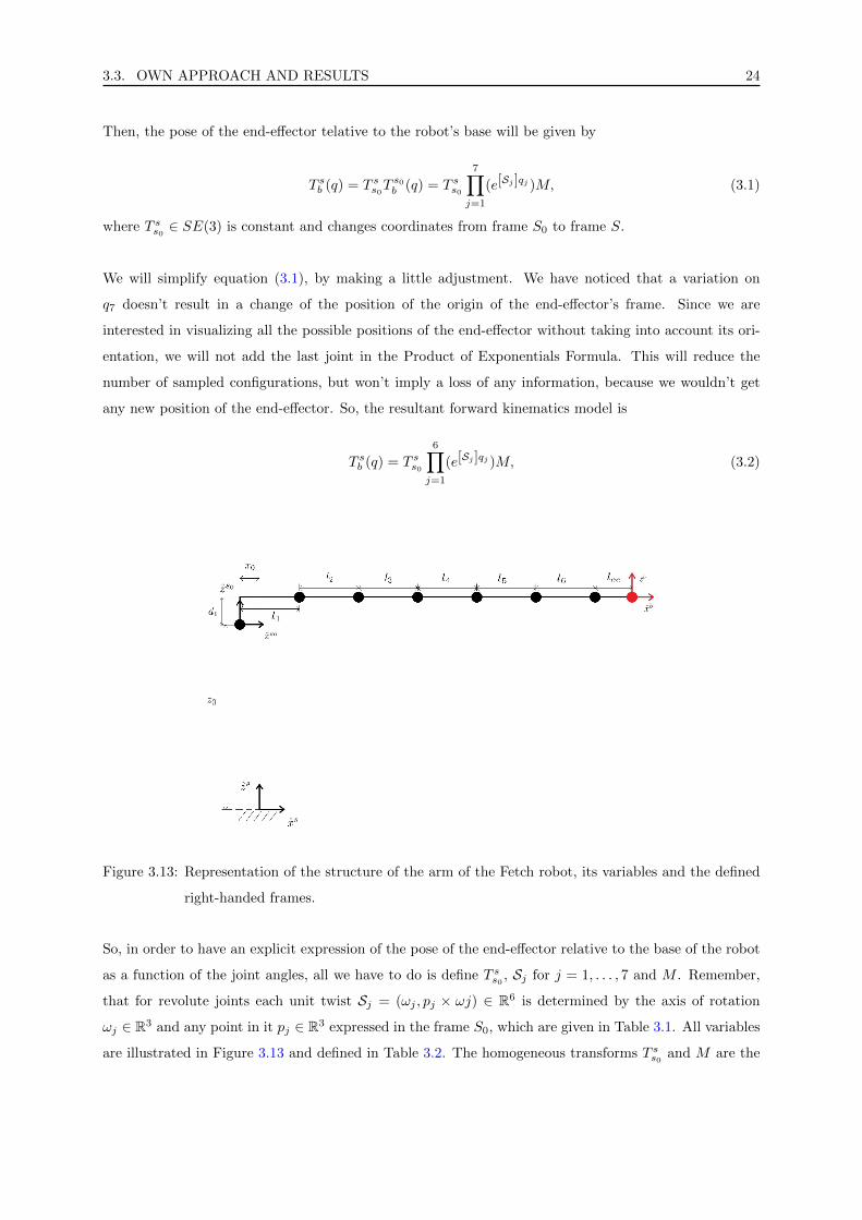
Then, the pose of the end-effector telative to the robot’s base will be given by
T sb (q) = T ss0Ts0b (q) = T ss0
7∏j=1
(e[Sj]qj )M, (3.1)
where T ss0 ∈ SE(3) is constant and changes coordinates from frame S0 to frame S.
We will simplify equation (3.1), by making a little adjustment. We have noticed that a variation on
q7 doesn’t result in a change of the position of the origin of the end-effector’s frame. Since we are
interested in visualizing all the possible positions of the end-effector without taking into account its ori-
entation, we will not add the last joint in the Product of Exponentials Formula. This will reduce the
number of sampled configurations, but won’t imply a loss of any information, because we wouldn’t get
any new position of the end-effector. So, the resultant forward kinematics model is
T sb (q) = T ss0
6∏j=1
(e[Sj]qj )M, (3.2)
Figure 3.13: Representation of the structure of the arm of the Fetch robot, its variables and the defined
right-handed frames.
So, in order to have an explicit expression of the pose of the end-effector relative to the base of the robot
as a function of the joint angles, all we have to do is define T ss0 , Sj for j = 1, . . . , 7 and M . Remember,
that for revolute joints each unit twist Sj = (ωj , pj × ωj) ∈ R6 is determined by the axis of rotation
ωj ∈ R3 and any point in it pj ∈ R3 expressed in the frame S0, which are given in Table 3.1. All variables
are illustrated in Figure 3.13 and defined in Table 3.2. The homogeneous transforms T ss0 and M are the

3.3. OWN APPROACH AND RESULTS 25
following:
T ss0 =
1 0 0 −x0
0 1 0 0
0 0 1 z0
0 0 0 1
(3.3)
M =
1 0 0 (l1 + l2 + l3 + l4 + l5 + l6 + lee)
0 1 0 0
0 0 1 d1
0 0 0 1
(3.4)
Joint ωj pj
1 (0, 0, 1) (0, 0, 0)
2 (0, 1, 0) (l1, 0, d1)
3 (1, 0, 0) (0, 0, d1)
4 (0, 1, 0) (l1 + l2 + l3, 0, d1)
5 (1, 0, 0) (0, 0, d1)
6 (0, 1, 0) (l1 + l2 + l3 + l4 + l5, 0, d1)
7 (1, 0, 0) (0, 0, d1)
Table 3.1: Values of the components of the unit twist Sj of each joint of the Fetch’s arm.
Variable name Values (m)
x0 0.0338
z0 0.98
d1 0.06
l1 0.117
l2 0.219
l3 0.133
l4 0.197
l5 0.125
l6 0.139
lee 0.166
Table 3.2: Values of the length variables of the structure of the Fetch’s arm.

3.3. OWN APPROACH AND RESULTS 26
3.3.2 Sampling
The sampling of the joint space has been done by discretizing the joint values intervals in an equidistant
way. Let m ∈ N be the number of values taken in each interval. Then, the number of total sampled
configurations is N = m7. We consider that, with m = 15, we should have enough different configurations
to obtain a good approach. Note that each sampled value of the j-th joint will beqmaxj −qmin
j
m−1 units away
from their adjacent values. The lower and upper limits of the j-th joint angle, qminj and qmaxj , are defined
in Table 3.3.
Joint qminj qmaxj
1 −π/2 π/2
2 −1.22 2.25
3 −π π
4 −2.25 2.25
5 −π π
6 −2.16 2.16
7 −π π
Table 3.3: Lower and upper joint limits of each joint on the Fetch’s arm.
Before obtaining the Cartesian coordinates of the end-effector’s position, we have reduced the number
of total configurations by eliminating the ones that correspond to a configuration in self-collision. This
process has been done by using the MoveIt Motion Planning Framework (MoveIt for short). For a given
set of joint values q ∈ Q, MoveIt allows us to check if the different robot parts are hitting each other in the
resultant configuration. Therefore, by repeating this test for each one of the sampled joint configurations,
we are able to discard the ones that would result in a self-collision state.
3.3.3 Reachable workspace
Now that we have our sampled set of joint configurations Qs ⊂ Q, we can obtain the pose of the end-
effector relative to the base frame for each configuration by substituting each q ∈ Qs in equation (3.2).
The result is an homogeneous transform represented as T sb = (Rsb , tsb) ∈ SE(3). To visualize the position
workspace in the Cartesian space, we have to plot each tsb = (t1, t2, t3) ∈ R3. The results are shown in
Figures 3.14, 3.15, 3.16 and 3.17.
To visualize the boundary of this cloud of sampled points, we have used pyvista and pygeo to generate
a 3D Triangulation mesh of the boundary. The resulting visualization of the workspace is illustrated in
Figures 3.18 and 3.19. Note that we can even perceive the robot’s silhouette.

3.3. OWN APPROACH AND RESULTS 27
Figure 3.14: A general view of the workspace representation of the Fetch’s arm expressed in the base
frame S.
Figure 3.15: Top view of the workspace representation of the Fetch’s arm expressed in the base frame S.
3.3.4 Constant orientation workspace
In this section, we will explain how to get an approach of the constant orientation workspace for an
arbitrary orientation of the end-effector and give the results for some specific orientations.
To visualize the constant orientation workspace in the Cartesian space, we have to select the end-effector’s

3.3. OWN APPROACH AND RESULTS 28
Figure 3.16: Front view of the workspace representation of the Fetch’s arm expressed in the base frame
S.
Figure 3.17: Side view of the workspace representation of the Fetch’s arm expressed in the base frame S.
poses T sb = (Rsb , tsb) ∈ SE(3) obtained in the previous section, whose Rsb ∈ SO(3) correspond to the goal
orientation and, then, plot the corresponding tsb = (t1, t2, t3) ∈ R3. Let xee, yee, zee ∈ R3 be three unit
orthogonal vectors, such that xee×yee = zee, denoting an arbitrary wanted orientation of the end-effector.
Then, the columns r1, r2, r3 of the rotation matrix Rsb have to be:
r1 = xee
r2 = yee
r3 = zee
(3.5)

3.3. OWN APPROACH AND RESULTS 29
Figure 3.18: Front view of the workspace’s boundary representation of the Fetch’s arm obtained with
pyvista and pygeo.
Figure 3.19: Side view of the workspace’s boundary representation of the Fetch’s arm obtained with
pyvista and pygeo.

3.3. OWN APPROACH AND RESULTS 30
For our case, we will take two considerations into account to select which poses present a correct ori-
entation. First, we will only analyze the direction of the x-axis of the end-effector’s frame B relative
to the base frame S. The study will be focused on xsb, because this is the direction towards which the
end-effector is pointing. We will lose control over ysb and zsb . But this will not be a problem, since the
last joint presents a full 360o rotation and a change on its value doesn’t change neither the end-effector’s
position nor xsb. So, with the origin and the x-axis fixed, we will be able to manipulate the last joint’s
angle to adjust the frame B as we want.
The second consideration that we are making is to allow some deviation of the end-effector’s sampled
orientations from the actual goal orientation. We have obtained the different joint configurations by
sampling, so the joint space is discretized. This makes very unlikely to result in the exact orientation
that we are looking for. So, we will approximate the constant orientation workspace by selecting all the
poses in which the end-effector’s pointing direction forms an angle with the desired direction less than or
equal to a limiting angle α.
To apply the idea of the limiting angle, we will use basic mathematics. It is well known, that given
two vectors u, v ∈ R3, the angle that they form can be obtained by the operation
· : R3 × R3 → (−π, π]
(u, v) 7→ uv = arccos〈u, v〉‖u‖‖v‖
,
where 〈·, ·〉 and ‖ · ‖ are the common scalar product and Euclidean norm of R3.
Now, we can establish the conditions that a Cartesian pose has to satisfy to be selected for our con-
stant orientation workspace approach. Let ω ∈ R3 be the desired pointing orientation of the end-effector
and α the limiting angle defined previously. Then, from equation (3.5) and the considerations that we
have made, an end-effector’s pose T sb = (Rsb , tsb) will be classified as valid for our constant orientation
workspace visualization if, and only if,
∣∣ωr1
∣∣ ≤ α (3.6)
is satisfied.
We have tested this process for different orientations with various limiting angles. The results for three
orientations with a limiting angle of α = 15o are presented. The plots correspond to the configurations
where the end-effector is facing forwards (Figure 3.20), to the left (Figure 3.21) and downwards (Figure
3.22).

3.3. OWN APPROACH AND RESULTS 31
Figure 3.20: Representation of the constant oriented workspace of the Fetch’s arm with the end-effector
facing forwards.
Figure 3.21: Representation of the constant oriented workspace of the Fetch’s arm with the end-effector
facing to the left.
Since our final goal is to choose the plane with a larger working surface of action given a direction for
the end-effector to face to, we will analyze the workspace in the planes, whose normal vector is equal to
the specified direction.
Like in the case of the orientation, we will allow a small error δ, that quantifies the maximum dis-
tance between a point and the studied plane, so that the point is considered to lie in the plane. The
reason to tolerate this error is the same as before: to work with a sampled cloud of points makes unlikely
that many points lie exactly in a concrete plane.
For each studied constant orientation workspace, we have intersected the cloud of points with several par-
allel planes, whose normal vector has the same direction as xsb and counted the number of included point
3.3. OWN APPROACH AND RESULTS 32
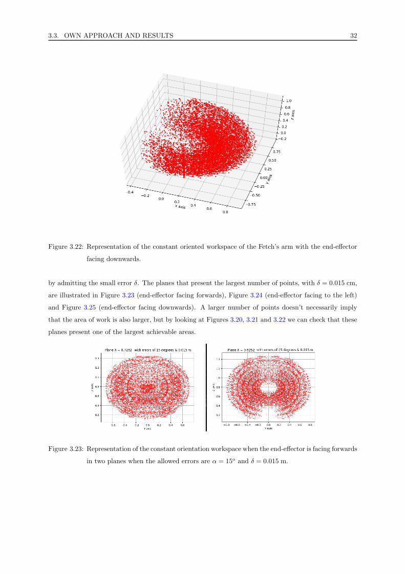
Figure 3.22: Representation of the constant oriented workspace of the Fetch’s arm with the end-effector
facing downwards.
by admitting the small error δ. The planes that present the largest number of points, with δ = 0.015 cm,
are illustrated in Figure 3.23 (end-effector facing forwards), Figure 3.24 (end-effector facing to the left)
and Figure 3.25 (end-effector facing downwards). A larger number of points doesn’t necessarily imply
that the area of work is also larger, but by looking at Figures 3.20, 3.21 and 3.22 we can check that these
planes present one of the largest achievable areas.
Figure 3.23: Representation of the constant orientation workspace when the end-effector is facing forwards
in two planes when the allowed errors are α = 15o and δ = 0.015 m.

3.3. OWN APPROACH AND RESULTS 33
Figure 3.24: Representation of the constant orientation workspace when the end-effector is facing to the
left in two planes when the allowed errors are α = 15o and δ = 0.015 m.
Figure 3.25: Representation of the constant orientation workspace when the end-effector is facing down-
wards in two planes when the allowed errors are α = 15o and δ = 0.015 m.

Chapter 4
Singularity analysis and visualization
Throughout the years, scientists have experienced issues when working with robots due to singularities.
For this reason, singularity states are undesired situations.
As we have announced in a previous chapter, manipulators lose at least one DoF when they reach
singularities. This is troublesome because velocities of the end-effector in some directions are not possi-
ble and may cause the robot to get stuck. Even when the manipulators are at configurations, that are
near to singularities, problems may appear, bacause very large joint motions are required to produce rel-
atively small end-effector’s displacements. Also, in the lab, we have experienced unexpected issues when
performing calligraphy and painting experiments with the manipulators, such as vibrations or weird and
apparently inefficient trajectories to move from a point to another that is very close to it.
In this chapter, we will analyze singularities for wrist-partitioned manipulators and present a method
to visualize them in a given plane.
4.1 Related work
An exhaustive research has been done on the previously done work related to singularity analysis of
manipulators. In this section, we present the part of this related work that is more useful for our purpose.
Kreutz-Delgado et al. [20] present a kinematic analysis of a 7R serial manipulator. To uniquely de-
termine the joint angles for a given end-effector’s pose, they introduce a parameter defined by the angle
between the arm plane and a reference plane. They give singularity conditions based on the values of
two scalar measures and classify the singular configurations depending on these conditions.
Tourassis and Ang [33] analyze the interplay between arm and wrist singularities and develop an in-
tuitive method for obtaining the manipulator’s singularities from the arm and wrist singularities. First
they decouple the singularities into the systems arm and wrist. They analyze both systems’ singulari-
34

4.2. DIRECTLY ACCESSIBLE WORKSPACE 35
ties separately and, then, obtain a formula that defines the manipulator’s singularities in terms of the
singularities of both systems. They conclude that singularities represent the boundaries between regions
with different number of solutions for the inverse kinematics problem. Their analysis leads to an efficient
method to identify the singularities of a 6R manipulator.
Decoupling the singularities of a wrist-partitioned manipulator into position and orientation singular-
ities is a frequently used way to determine the singularity sets. In the following sections, we will analyze
this method in detail. The main advantage of this method, is that, by choosing the end-effector’s frame
properly, the analysis can be simplified. Hayes et al. [16] decouple the singularities to analytically de-
scribe and classify the singularities of wrist-partitioned 6R serial manipulators in general and apply it
to a specific robot. Cheng et al. [9] also apply the decoupling method to analyze the singularities of
redundant 7-DoF manipulators. They give conditions on the joint values and classify the singularities.
Additionally, they compare singularity avoidance methods and present their own. Unlike other existing
method, their method considers the position singularities and the orientation singularity separately and
it can avoid escapable singularities of redundant manipulators efficiently and effectively. Xu et al. [36]
combine the singularity decoupling method with a damped reciprocal method, in order to manipulate a
spacecraft with a wrist-partitioned manipulator.
Goyal and Sethi [12] and Abdel-Malek et al. [1] present methods to determine the position singularities
of serial manipulators that present joint limits. They create three singularity compound of joint configu-
rations sets by applying a row-rank deficiency criterion and considering the joint limits. To parametrize
the position singularity surfaces they substitute the singularity sets into the forward kinematics formula.
Bedrossian [3] presents a method for the analysis of singularities of redundant manipulators. He classifies
the singularities according to whether reconfiguration into a non-sigular posture is possible using null
motion, i.e. a motion that doesn’t disturb the end-effector’s location. He gives necessary and sufficient a
null vector has to satisfy to be admissible.
Haug et al. [15] analyzes the singularities of planar and spatial manipulators by using first and second
order Taylor approximations of the output variables in selected directions as functions of manipulator
input variables. They classify the singularities into boundary barriers, interior barriers and crossable
singularities.
4.2 Directly accessible workspace
In his thesis [22], Kunze defines the directly accessible workspace. Unlike the reachable workspace, which
is the set of all poses that the end-effector can achieve, the directly accessible workspace is the set of
poses that the end-effector can reach from its current pose in a straight motion.

4.2. DIRECTLY ACCESSIBLE WORKSPACE 36
This concept may help us understand the source of the unexpected behaviour of the robot, when per-
forming not intuitive movements to move between to points that are very close to each other. Sometimes,
a position may be very close to the end-effector’s current position, but not lie in the directly accessible
workspace. It is in these cases, when the manipulator requires to perform a large reconfiguration to
reach the goal end-effector’s pose. The simple 2R planar example in Figure 4.1 may be helpful in the
comprehension of these situations.
Figure 4.1: Illustration of the directly accessible workspace (green) and the reachable workspace (light
red) of a 2R planar manipulator with joint limits. The blue cross is the goal position. It
is very very close to the current end-effector’s position, but it does not lie in the directly
accessible workspace. The manipulator needs a large reconfiguration to reach the goal pose.
Source: [22].
Kunze presents a method to approximate the directly accessible workspace. He samples directions in
the three-dimensional Euclidean space and traces rays from the end-effector’s position in each sampled
direction. Then, he samples points in each ray. The distance between two consecutive points is directly
proportional to their distance to the end-effector. For each ray, he computes the inverse kinematics prob-
lem for the closest point to the end-effector. If there is not a solution or a joint limit is hit the point will
be considered as the last feasible one. If none of these conditions is satisfied the process is repeated for
the next ppoint in the ray. Finally the boundary of the directly accessible workspace is approximated
with the last feasible point of each ray. Again, to facilitate the comprehension of how the method works,
a 2R planar example is illustated in Figure 4.2.

4.3. DECOUPLING OF WRIST-PARTITIONED MANIPULATORS 37
Figure 4.2: Illustration of the approximation of the directly accessible workspace (green) obtained with
Kunze’s method and the actual directly accessible workspace(light green). The rays are traced
in the sampled directions and points are sampled in each ray. The the set of last feasible
points on each ray delimits the boundary of the approximation. Source: [22].
4.3 Decoupling of wrist-partitioned manipulators
In this section, we will see how we can simplify the analysis of singularities of wrist-partitioned manipu-
lators by using the workspace decomposition method presented in [29].
Hollerbach and Sahar [17] and Megahed [24] analyze the kinematics of wrist-partitioned manipulators.
The present a method to obtain the inverse kinematics position of the end-effector by decoupling the
wrist-partitioned manipulator into the forearm and the wrist. The 1st and 2nd time derivatives of the
obtained models by Megahed give more accurate inverse kinematic velocity and acceleration models than
numerical differentiation. The method consists of the following steps:
1. Find the wrist position.
2. Find the joint angles of the forearm.
3. Find the orientation of the end-effector relative to the forearm.
4. Find the wrist joint angles.
Cheng et al. [9] use the workspace decomposition method to decouple analyze the singularities of a 7
DoF redundant manipulator. The singularities are decoupled into position singularities and orientation

4.3. DECOUPLING OF WRIST-PARTITIONED MANIPULATORS 38
singularities. Then, the joints are divided into two sets: the forearm (first four joints) and the wrist (last
three joints).
The key to decouple the singularity into position singularities and orientations singularities is to se-
lect the velocity reference point at the center of the wrist. Remember that the relationship between the
joint rates q and the end-effector velocities V is given by the Jacobian manipulator J(q):
Vee = J(q)q (4.1)
Unlike we have done before, in [29] and [9], the end-effector’s twist is defined as
Vee =
veeωee
∈ R6. (4.2)
Since the results are independent of the twist’s definition, we will adopt theirs.
In [29], it is proven that, if the velocity reference point is selected at the wrist center, the resulting
Jacobian matrix has the form
JW =
J11 0
J21 J22
(4.3)
where, for a 7 DoF manipulator, J11, J21 ∈ R3×4 and J22 is a square matrix of order 3.
The resulting singularity sets will be the same, since, as we have already seen, the singularity condi-
tion is that the Jacobian matrix isn’t full-rank and the rank of the Jacobian does not depend on the
chosen velocity reference point.
Now, if we define
q =
qfaqw
(4.4)
where,
qfa =
q1
q2
q3
q4
(4.5)
and
qw =
q5
q6
q7
, (4.6)

4.3. DECOUPLING OF WRIST-PARTITIONED MANIPULATORS 39
then the relationship between joint rates and the wrist’s velocities can be rewritten as
VW =
vwωw
= JW q =
J11 0
J21 J22
qfaqw
(4.7)
Intuitively, it can be seen as the incapability of the last three joints to change the wrist center’s position.
The condition for the manipulator to be in a singularity state is
rank(JW ) < 6. (4.8)
But, now that we have rewritten the problem, the whole set of singularities can be divided into posi-
tion singularities and orientation singularities. We will present this singularity types in the following
subsections.
4.3.1 Position singularities
As the linear velocities vw are only affected by the forearm (4.7), the position singularites only depend
on the first four joints. Hence, the conditions for the position singularities will be given by
det(J11JT11) = 0. (4.9)
But, equation (4.9) doesn’t take joint limits into account. Goyal and Sethi [12] and Abdel-Malek et al. [1]
propose two very similar methods to determine the reachable workspace and the singularity surfaces by
also considering joint limits. They obtain three different singularity sets with the correspondent conditions
on the joint values. Then, they parameterize the singularity surfaces by substituting the singularity sets
into the kinematic constraint equations. The results obtained by Abdel-Malek et al. for a RPRP forearm
are shown in Figures 4.3 and 4.4.
Figure 4.3: Representation of the singularity and boundary surfaces obtained by Abdel-Malek et al. for
a RPRP manipulator. Source: [1]
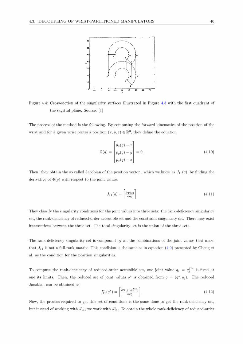
4.3. DECOUPLING OF WRIST-PARTITIONED MANIPULATORS 40
Figure 4.4: Cross-section of the singularity surfaces illustrated in Figure 4.3 with the first quadrant of
the sagittal plane. Source: [1]
The process of the method is the following. By computing the forward kinematics of the position of the
wrist and for a given wrist center’s position (x, y, z) ∈ R3, they define the equation
Φ(q) =
px(q)− x
py(q)− y
pz(q)− z
= 0. (4.10)
Then, they obtain the so called Jacobian of the position vector , which we know as J11(q), by finding the
derivative of Φ(q) with respect to the joint values.
J11(q) =
[∂Φ(q)∂qj
](4.11)
They classify the singularity conditions for the joint values into three sets: the rank-deficiency singularity
set, the rank-deficiency of reduced-order accessible set and the constraint singularity set. There may exist
intersections between the three set. The total singularity set is the union of the three sets.
The rank-deficiency singularity set is compound by all the combinations of the joint values that make
that J11 is not a full-rank matrix. This condition is the same as in equation (4.9) presented by Cheng et
al. as the condition for the position singularities.
To compute the rank-deficiency of reduced-order accessible set, one joint value qj = qfixj is fixed at
one its limits. Then, the reduced set of joint values q∗ is obtained from q = (q∗, qj). The reduced
Jacobian can be obtained as
J∗11(q∗) =
[∂Φ(q∗,qfix
j )
∂q∗j
]. (4.12)
Now, the process required to get this set of conditions is the same done to get the rank-deficiency set,
but instead of working with J11, we work with J∗11. To obtain the whole rank-deficiency of reduced-order

4.4. VISUALIZATION 41
accessible set, the process must be repeated for all the joints that present joint limits.
The constraint singularity set is formed by all the combinations of q = (q∗∗, qfixi , qfixj ), ∀i, j ∈ N, such
that 1 ≤ i < j ≤ n, where n is the number of joints in the forearm and the i-th and the j-th joint are
fixed at one of their limits.
Once all the sets are created, they are substituted in equation (4.10) to obtain a parameterization of
the singularity surfaces and, finally, visualize them.
4.3.2 Orientation singularities
The angular velocity ωw is affected by both the forearm and the wrist (4.7). Hence, the conditions for
the orientation singularities are determined by
rank( [J21 J22
] )< 3. (4.13)
Equation (4.13) is subject to the following three subconditions:
i. Forearm orientation singularity:
det(J21JT21) = 0. (4.14)
ii. Wrist orientation singularity or simply wrist singularity:
det(J22) = 0. (4.15)
iii. Combined orientation singularity: Even if the first two subconditions are satisfied, there may still
be the chance to find 3 independent columns between J21 and J22. By not allowing this possibility,
we get the combined orientation singularity condition.
It is important to know, that the manipulator will be at an orientation singularity state when the three
subconditions are satisfied simultaneously.
4.4 Visualization
For the visualization of the singularity sets we will use the CuikSuite [25]. The CuikSuite is a set of
applications to solve position analysis and path planning problems with applications mainly to robotics,
such use the computation and visualization of singularities in both the joint space and the Cartesian space.
The CuikSuite’s computation and visualization of the singularity sets is done by applying the methods
presented by Bohigas in his PhD thesis [4]. The proposed method for the computation of the singularities
is a branch-and-prune method.

4.4. VISUALIZATION 42
We will now see, how Bohigas addresses the kinematic analysis of a manipulator. All the possible
configurations of a manipulator can be characterized by a non-linear system of equations that expresses
the assembly constraints imposed by the joints,
Φ(q) = 0. (4.16)
Additionally, for a given configuration it is possible to find a velocity equation,
L(q) m = 0, (4.17)
that gives all possible motions of the manipulator for that configuration. m is a velocity vector, which
globally characterizes the velocity state of the manipulator. Bohigas distinguishes three subvectors in
m =[mu,mv,mp
]. mu are the output velocities (typically the end-effector’s twist), mv the input veloci-
ties (i.e. the velocities of the actuated joints) and mp the passive velocities.
Bohigas classifies the whole set of singular configurations into forward singularities and inverse singu-
larities. The forward instantaneous kinematics problem (FIKP) consist on finding the velocity vector,
m, given an input velocity vector, mv. On the other hand, the inverse instantaneous kinematics problem
(IIKP) consist on finding the velocity vector, m, given an ouput velocity vector, mu. Forward and inverse
kinematics are given when these problems become indeterminate.
Bohigas shows, that the forward and inverse singularities can be characterized by the following systems
of equations:
Φ(q) = 0
Ly(q) ξ = 0
‖ξ‖2 = 1
, (4.18)
Φ(q) = 0
Lz(q) ξ = 0
‖ξ‖2 = 1
. (4.19)
The first line in the systems of equations (4.18) and (4.19) constrains the joint values vector q to be a
valid configuration. The last two lines, impose the rank-deficiency of the matrices Ly(q) and Lz(q). Ly(q)
and Lz(q) are obtained from the matrix L(q) in equation (4.17), by removing the removing the columns
corresponding to mv and mu, respectively.
Bohigas proposes to use a branch-and-prune method for the resolution of the systems of equations (4.18)
and (4.19). These methods are based on exclusion. An initial box bounding the whole set of solutions
B is required. Then, they iteratively remove portions of B that don’t contain any solutions, until the
remaining boxes are considered to be a fine enough approximation of the solution.

4.4. VISUALIZATION 43
To converge to all the solutions, the algorithm recursively applies two operations on B: box shrink-
ing and box splitting. The boxes are shrinked by narrowing some of their defining intervals and portions
of B that don’t present any solution are excluded. The shrinking process is repeated until either the
box is reduced to an empty set (i.e. it contains no solution), or the box is considered sufficiently small
and, therefore, a solution box (i.e. it is considered as a fine enough approximation of a solution) or the
box cannot be “significantly” reduced, in which case the splitting box operation is applied to bisect the
largest interval of the box and splits the box into two sub-boxes. The progression of the algorithm on
finding the solutions to an example equation is illustrated in Figure 4.5.
Figure 4.5: Progression of the branch-and-prune algorithm on finding the solutions to the equation y4 =
y2 − x2. The initial box is the bounding box cointaining the solutions and the solutions are
given by the curve described by the small solution boxes. Source: [4].
Before applying the branch-and-prune algorithm to the systems of equations (4.18) and (4.19), Bohigas
shows that they can be rewritten as a larger system of equations
Λ(x) = 0
Ω(x) = 0
, (4.20)
where Λ(x) is a sub-system of linear equations and Ω(x) is a sub-system of quadratic equations. Once
the problem is rewritten as the system of equations (4.20), the algorithm is more easily applied to find
4.5. OWN APPROACH AND RESULTS 44
their solutions.
The CuikSuite presents applications to apply the methodology introdued by Bohigas. For a given ma-
nipulator, it allows to directly obtain the system of equations (4.20), by just giving a definition of the
manipulator’s environment and structure. Then, the branch-and-prune algorithm can be applied to ob-
tain the set of solution boxes. Finally, the solutions can be visualized either in the joint space or the
output space.
4.5 Own approach and results
We propose a method to analyze and compute the singularities of a wrist-partitioned manipulator that
combines the singularity decoupling method for wrist-partitioned manipulators and the branch-and-prune
algorithm presented by Bohigas [4] to compute the resolution of the position singularity system of equa-
tions.
By decoupling the Fetch into forearm and wrist, we can separate the joint values into qfa = [q1, q2, q3, q4]T
and qw = [q5, q6, q7]T
. From section 4.3, we know that the study of position singularities will be restricted
to qfa, while the study of the orientation singularities will consider all the joints.
4.5.1 Position singularities
The first step of our method is to compute the forward kinematics of the forearm. We define the reference
frames S and the wrist frame W , both with the same orientation. The origin of the S frame is located
at the first joint and the origin of W is located at the wrist center. S and W are shown in Figure 4.6.
Again, we obtain the forward kinematics by applying the Product of Exponentials Formula
T sw(qfa) =
4∏j=1
(e[Sj]qj )MW , (4.21)
where
M =
1 0 0 (l1 + l2 + l3 + l4 + l5)
0 1 0 0
0 0 1 d1
0 0 0 1
, (4.22)
and the structure parameters, the joint limits and the components of the unit twists are the same pre-
sented in Table 3.2, in Table 3.3 and Table 3.1, respectively.

4.5. OWN APPROACH AND RESULTS 45
Figure 4.6: 3D visualization of the Fetch Mobile Manipulator using rviz. The reference frame and the
wrist frame are illustrated. The red axes are the x-axes, the green axes are the y-axes and
the blue axes are the z-axes.
By using the obtained position of the wrist we can write the assembly constraints as
Φ(q) =
tx(q)− x
ty(q)− y
tz(q)− z
= 0. (4.23)
Then, Φ(qfa) can be derived with respect the forearm joint values to obtain the matrix J11. The system
of equations with which Bohigas characterizes the singularities, in our case can be written as
Φ(qfa) = 0
J11(qfa) ξ = 0
‖ξ‖2 = 1
. (4.24)
Since we want to visualize the position singularities in a given plane of action of the wrist, we will add
the equation of the plane to the system to constrain the position of the wrist to the mentioned plane.
The resulting system of equations is
Φ(qfa) = 0
J11(qfa) ξ = 0
‖ξ‖2 = 1
ax+ by + cz + d = 0
. (4.25)

4.5. OWN APPROACH AND RESULTS 46
The next step is to extend this system of equation into a system of linear and quadratic equations like
Bohigas does.
Finally, the branch-and-prune algorithm is applied to the system of linear and quadratic equations to
obtain the solutions of the system, and, therefore the set of joints values that correspond to a position
singularity state in the specified plane. To obtain the Cartesian coordinates of these singularities, the
forward kinematics (4.21) have to be computed.
In order to obtain the system of equations (4.24), we have defined the structure and environment of
the Fetch’s forearm. The CuikSuite is able to obtain the system of equations. Then, we can add the
plane’s equation to the system and use CuikSuite to apply the branch-and-prune algorithm to find its
solutions. Finally, after the solutions have been generated, CuikSuite allow us to visualize them.
Unfortunately, the computation of this algorithm is very expensive and so is the required memory. Due to
the current situation that we are living because of the COVID-19 world pandemic, we don’t have access
to an enough powerful computer. The program breaks will running during memory issues when we run
it in our computer.
To show the potential of the CuikSuite, we will visualize the singularities of a simpler manipulator:
Figure 4.7 shows the obtained singularities of a planar 3R manipulator. In Appendix A, it is shown how
the .world files have to be in order to define serial manipulators and the CuikSuite’s commands that have
to be run to visualize their singularities.
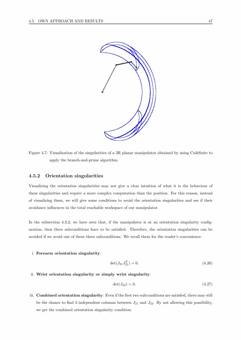
4.5. OWN APPROACH AND RESULTS 47
Figure 4.7: Visualization of the singularities of a 3R planar manipulator obtained by using CuikSuite to
apply the branch-and-prune algorithm.
4.5.2 Orientation singularities
Visualizing the orientation singularities may not give a clear intuition of what it is the behaviour of
these singularities and require a more complex computation than the position. For this reason, instead
of visualizing them, we will give some conditions to avoid the orientation singularities and see if their
avoidance influences in the total reachable workspace of our manipulator.
In the subsection 4.3.2, we have seen that, if the manipulator is at an orientation singularity config-
uration, then three subconditions have to be satisfied. Therefore, the orientation singularities can be
avoided if we avoid one of these three subconditions. We recall them for the reader’s convenience:
i. Forearm orientation singularity:
det(J21JT21) = 0. (4.26)
ii. Wrist orientation singularity or simply wrist singularity:
det(J22) = 0. (4.27)
iii. Combined orientation singularity: Even if the first two subconditions are satisfied, there may still
be the chance to find 3 independent columns between J21 and J22. By not allowing this possibility,
we get the combined orientation singularity condition.

4.5. OWN APPROACH AND RESULTS 48
We will see how we can avoid the wrist singularity. In [29], it is proven that the wrist singularity happens
when the unit vectors describing the rotation axes of the wrist joints are linearly dependent. This situation
can only be given when the first and the last joint (z5 and z7 in our case) are collinear. This just happens
when the wrist flex joint value is zero (q6 = 0 in our case). Figure 4.8 illustrates the configuration of the
wrist in the wrist singularity state.
Figure 4.8: Wrist singularity configuration. The rotation axes z5 and z7 are collinear. z6 is the axis of
rotation of the wrist flex joint.
Our question now is if we are able to avoid the orientation singularities without losing volume of workspace.
In order to avoid the wrist singularity, and consequently the orientation singularities, we will constraint
the wrist flex joint q6 to strictly positive or strictly negative values. Figures 4.9 and 4.10 show the resulting
workspace of the Fetch by applying this restrictions. By comparing both figures, we can see how the
generated workspace is very similar. By comparing them with Figure 3.18, the workspace also looks
similar. So, we can conclude that we can avoid the orientation singularities without losing a significant
amount of the workspace’s volume, from the point of view of the position, in the process.

4.5. OWN APPROACH AND RESULTS 49
Figure 4.9: Workspace of the Fetch with the wrist flex joint constrained only to negative values.
Figure 4.10: Workspace of the Fetch with the wrist flex joint constrained only to positive values.
Chapter 5
Conclusions
In this thesis, several methods for workspace determination of a serial spatial manipulator have been
presented. The visualization of the workspace of a 7-DoF wrist-partitioned manipulator has been succes-
sively achieved through a forward kinematics approach.
A methodology to obtain the constant orientation workspace of a serial manipulator has been presented.
An approximation of the constant orientation workspace of a wrist-partitioned redundant manipulator
has been obtained and visualized, for some specific orientations.
A method to compute the position singularities of a wrist-partitioned manipulator in a specific plane
has been presented, motivated by the need of finding the largest singularity free surface on the given
plane. The method is the result of a combination of a decoupling singularity method and a branch-
and-prune method for the resolution of systems of equations. Unfortunately, the visualization of the
singularity sets obtained by the method has not been achieved, due to the lack of a powerful enough
computer.
A way to avoid the orientation singularities of a wrist-partitioned manipulator by avoiding the wrist
singularity type has been presented. It has been shown, that the set of positions that the end-effector
can reach is not significantly reduced, when avoiding the orientation singularities.
50

Chapter 6
Future work
In this chapter, some further research directions that can be useful to extend the desired working area in
a given plane of action and in the graffiti painting project.
6.1 Test results on the physical robot
Unfortunately, the outbreak of the COVID-19 world pandemic has precluded us to test our results with
the actual Fetch robot. So the first thing to do in the future would be to constrain the movements of the
Fetch with our results and check if we have avoided the vibrations and weird trajectories.
6.2 Mobile manipulation
A very intuitive idea to extend the workspace of a manipulator, is to mount it on a mobile platform.
The wheels would allow the base of the robot to move along the ground plane. If the reference frame is
attached to the mobile, the singularity analysis problem for the manipulator would be the same at each
instant of time, just that the workspace would be displaced.
For the graffiti painting case, the wheeled base could be used to move parallel to the wall. In this
way, the plane of action could be infinitely extended, with the movement of the manipulator still con-
straint in a singularity free region. For example, the Fetch has non-steered wheels. So if the end-effector
is facing side wards, the Fetch would be able to move back and forth while painting without having to
rotate about itself.
6.3 Crossable and non-crossable singularity sets
Work has been done related to the analysis of the crossability of the singularity sets [15, 2]. Some of
the singularity sets allow motion across them in any direction, these singularities are called crossable
singularities. The rest of singularities are non-crossable. A clear example for a non-crossable singularity
51

6.4. SPRAY CAN MANIPULATION 52
would be the boundary surface, since it is obvious that the end-effector can’t cross it and reach a point
out of the workspace.
A complete classification of all singularities into crossable and non-crossable may result in a larger work-
ing area of work if we are willing to freely move over the crossable singularities. But a more detailed
study would be required, because even if they are crossable, they are still singularities as their name
suggests.
6.4 Spray can manipulation
Since the work done in this thesis has been part of a graffiti painting project, it would be interesting to
study how we could grasp efficiently a spray can with the Fetch manipulator and manipulate it properly,
in order to paint quality graffitis.

Appendices
53

Appendix A
The CuikSuite
In this appendix, it will be shown how the CuikSuite can be used in order to visualize the singular
configurations of a manipulator.
A.1 Description and examples of .world files
Before we are able to use the CuikSuite to compute the singularity equations of a manipulator and visu-
alize their solutions, it is required that we define the environment and the structure of the manipulator.
All this information is gathered in the .world files.
The .world files are used to describe the links and joints of the manipulator and to establish the re-
lationship between them. In Listings A.1 and A.2, these type of files for the 3R planar manipulator’s and
the Fetch’s forearm’s cases are presented .
1 [CONSTANTS]
2
3 l1:=4
4 l2:=2
5 l3:=1
6
7 range1_low :=-pi/3
8 range2_low :=-pi/3
9 range3_low :=-pi/3
10
11 range1_up :=pi/3
12 range2_up :=pi/3
13 range3_up :=pi/3
14
15 [LINKS]
16
17 base: sphere 0.1 (0,0,0) red
54

A.1. DESCRIPTION AND EXAMPLES OF .WORLD FILES 55
18
19 link1: color (0.9 ,0.9 ,0.9)
20 cylinder 0.05 (0,0,0) (l1 ,0,0)
21 sphere 0.1 (l1 ,0,0) red
22
23 link2: color (0.1 ,0.1 ,0.1)
24 cylinder 0.05 (0,0,0) (l2 ,0,0)
25 sphere 0.1 (l2 ,0,0) red
26
27 link3: color (0.9 ,0.9 ,0.9)
28 cylinder 0.05 (0,0,0) (l3 ,0,0)
29
30 end_effector: sphere 0.1 (0,0,0) green
31
32 [JOINTS]
33 revolute: base (0,1,0) (0,-1,0) % P_1 and Q_1 defining the rotation
34 % axis in the ground frame
35 link1 (0,1,0) (0,-1,0) % P_2 and Q_2 defining the rotation
36 % axis in the link1 frame
37 range [range1_low ,range1_up] % Joint limits
38 +(1,0,0) +(1,0,0) % Two points R_1 and R_2 defining two
39 % vectors P_1 ->R_1 P_2 ->R_2 that coincide
40 % when the rotation is 0
41
42 revolute: link1 (l1 ,1,0) (l1 ,-1,0)
43 link2 (0 ,1,0) (0 ,-1,0)
44 range [range2_low ,range2_up]
45 +(1,0,0) +(1,0,0)
46
47
48 revolute: link2 (l2 ,1,0) (l2 ,-1,0)
49 link3 (0 ,1,0) (0 ,-1,0)
50 range [range3_low ,range3_up]
51 +(1,0,0) +(1,0,0)
52
53 fix: link3 end_effector
54 Tx(l3)
Listing A.1: .world of the 3R planar manipulator.
Now, we will see how to define links and joints in the .world files. Links are represented by a geometrical
figure. For example, in the 3R planar case, they are represented by a cylinder. The diameter and the
beginning and ending points of the cylinder define a link. The spheres attached to each link are a visual
representation of the joint. To define the joints their limits and three pairs of points are required. The
first pair (P1 and Q1 in Listing A.1), define the axis of rotation in the frame of the parent link. The
second pair (P2 and Q2 in Listing A.1), define the axis of rotation in the frame of the child link. The last
pair of points (R1 and R2 in Listing A.1) are used to establish when the rotation is null. The segments
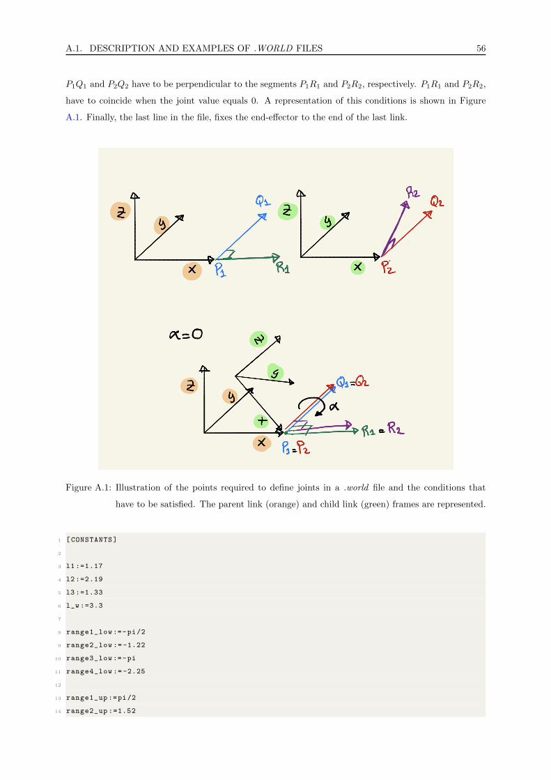
A.1. DESCRIPTION AND EXAMPLES OF .WORLD FILES 56
P1Q1 and P2Q2 have to be perpendicular to the segments P1R1 and P2R2, respectively. P1R1 and P2R2,
have to coincide when the joint value equals 0. A representation of this conditions is shown in Figure
A.1. Finally, the last line in the file, fixes the end-effector to the end of the last link.
Figure A.1: Illustration of the points required to define joints in a .world file and the conditions that
have to be satisfied. The parent link (orange) and child link (green) frames are represented.
1 [CONSTANTS]
2
3 l1 :=1.17
4 l2 :=2.19
5 l3 :=1.33
6 l_w :=3.3
7
8 range1_low :=-pi/2
9 range2_low := -1.22
10 range3_low :=-pi
11 range4_low := -2.25
12
13 range1_up :=pi/2
14 range2_up :=1.52

A.1. DESCRIPTION AND EXAMPLES OF .WORLD FILES 57
15 range3_up :=pi
16 range4_up :=2.25
17
18 [LINKS]
19
20 base: sphere 0.1 (0,0,0) red
21
22 link1: color (0.9 ,0.9 ,0.9)
23 cylinder 0.05 (0,0,0) (l1 ,0,0)
24 sphere 0.1 (l1 ,0,0) red
25
26 link2: color (0.1 ,0.1 ,0.1)
27 cylinder 0.05 (0,0,0) (l2 ,0,0)
28 sphere 0.1 (l2 ,0,0) red
29
30 link3: color (0.9 ,0.9 ,0.9)
31 cylinder 0.05 (0,0,0) (l3 ,0,0)
32 sphere 0.1 (l3 ,0,0) red
33
34 link4: color (0.9 ,0.9 ,0.9)
35 cylinder 0.05 (0,0,0) (l_w ,0,0)
36
37 wrist: sphere 0.1 (0,0,0) green
38
39 [JOINTS]
40 revolute: base (0,0,0) (0,0,1)
41 link1 (0,0,0) (0,0,1)
42 range [range1_low ,range1_up]
43 +(1,0,0) +(1,0,0)
44
45 revolute: link1 (l1 ,0,0) (l1 ,1,0)
46 link2 (0,0,0) (0,1,0)
47 range [range2_low ,range2_up]
48 +(1,0,0) +(1,0,0)
49
50
51 revolute: link2 (l2 ,0,0) (l2+1,0,0)
52 link3 (0,0,0) (1,0,0)
53 range [range3_low ,range3_up]
54 +(0,1,0) +(0,1,0)
55
56 revolute: link2 (l3 ,0,0) (l3 ,1,0)
57 link3 (0,0,0) (0,1,0)
58 range [range3_low ,range3_up]
59 +(1,0,0) +(1,0,0)
60
61 fix: link4 wrist

A.2. SINGULARITY DETERMINATION COMMANDS 58
62 Tx(l_w)
Listing A.2: .world of the Fetch’s forearm.
A.2 Singularity determination commands
In this section, we will see the commands that we have to run in order to visualize the singularities of a
manipulator. In particular, we will show the commands used to obtain the results shown in 4.7.
We will suppose that the file is called 3R.world and it is located in a folder named Manipulators. The
commands are shown in Listing A.3. To run first command it is important that in the .param file it
is specified that the representation is done by links with the line REPRESENTATION = LINKS. The
.param also contains other parameters, such as the ones used by the btanch-and-prune algorithm.
1 $ cuiksingequations Manipulators /3R
2 $ cuiksimplify Manipulators /3 R_sing
3 $ cuikaddjacobian Manipulators /3 R_sing_simp end_effector_r_x end_effector_r_z
4 $ cuik Manipulators /3 R_sing_simp_J
5 $ cuikplot3d Manipulators /3 R_sing_simp_J 9 11 10 0 workspace3R
6 $ cuikmove Manipulators /3R
Listing A.3: CuikSuite commands used to obtain the results shown in Figure 4.7.
The first three commands generate a .cuik file containing the singularity system of equations. The cuik
command creates a .sol file containing the solutions to the system of equations. A .gcl file containing a 3D
representation of the solutions is created with the cuikplot3d command. Finally, the cuikmove command
can be used to visualize and move the manipulator with visualizer geomview and the singularities can be
visualized by loading the generated file workspace3R.gcl.

Bibliography
[1] K. Abdel-Malek, F. Adkins, H.-J. Yeh, and E. Haug. On the determination of boundaries to manip-
ulator workspaces. Robotics and Computer-Integrated Manufacturing, 13(1):63–72, 1997.
[2] K. Abdel-Malek and H.-J. Yeh. Crossable surfaces of robotic manipulators with joint limits. Journal
of Mechanical Design, 122(1):52–60, 2000.
[3] N. S. Bedrossian. Classification of singular configurations for redundant manipulators. IEEE Inter-
national Conference on Robotics and Automation, pages 818–823, 1990.
[4] O. Bohigas. NUMERICAL COMPUTATION AND AVOIDANCE OF MANIPULATOR SINGU-
LARITIES. PhD thesis, Universitat Politecnica de Catalunya (UPC), 2013.
[5] Y. Cao, S. Qi, K. Lu, Y. Zang, and G. Yang. An integrated method for workspace computation of
robot manipulator. International Joint Conference on Computational Sciences and Optimization,
1:309–312, 2009.
[6] Y. Cao, H. Zang, L. Wu, and T. Wu. An engineering-oriented method for the three dimensional
workspace generation of robot manipulator. Journal of Information and Computational Science,
8(1):51–61, 2011.
[7] Gianni Castelli, Erika Ottaviano, and Marco Ceccarelli. A fairly general algorithm to evaluate
workspace characteristics of serial and parallel manipulators. Mechanics based design of structures
and machines, 36(1):14–31, 2008.
[8] M. Ceccarelli. A formulation for the workspace boundary of generaln-revolute manipulators. Mech-
anism and Machine Theory, 31(5):637–646, 1996.
[9] F.-T. Cheng, J.-S. Chen, and F.-C. Kung. Study and resolution of singularities for a 7-dof redundant
manipulator. IEEE Transactions on Industrial Electronics, 45(3):469–480, 1998.
[10] G. S. Chirikjian and I. Ebert-Uphoff. Discretely actuated manipulator workspace generation using
numerical convolution on the euclidean group. IEEE International Conference on Robotics and
Automation, 1:742–749, 1998.
[11] G. S. Chirikjian and I. Ebert-Uphoff. Numerical convolution on the euclidean group with applications
to workspace generation. IEEE Transactions on Robotics and Automation, 14(1):123–136, 1998.
59

BIBLIOGRAPHY 60
[12] K. Goyal and D. Sethi. An analytical method to find workspace of a robotic manipulator. Journal
of Mechanical Engineering, 41(1):25–30, 2010.
[13] Y. Guan and K. Yokoi. Reachable space generation of a humanoid robot using the monte carlo
method. IEEE/RSJ International Conference on Intelligent Robots and Systems, pages 1984–1989,
2006.
[14] J. A. Hansen, K. C. Gupta, and S. M. K. Kazerounian. Generation and evaluation of the workspace
of a manipulator. The International Journal of Robotics Research, 2(3):22–31, 1983.
[15] E. J. Haug, F. A. Adkins, C. C. Qiu, and J. Yen. Analysis of barriers to control of manipulators within
accessible output sets. In Proceedings of the 20th ASME Design Engineering Technical Conference,
pages 82–697, 1995.
[16] M. J. D. Hayes, M. L. Husty, and P. J. Zsombor-Murray. Singular configurations of wrist-partitioned
6r serial robots: a geometric perspective for users. Transactions of the Canadian Society for Me-
chanical Engineering, 26(1):41–55, 2003.
[17] J. M. Hollerbach and G. Sahar. Wrist-partitioned, inverse kinematic accelerations and manipulator
dynamics. The International Journal of Robotics Research, 2(4):61–67, 1983.
[18] L. Jamone, L. Natale, K. Hashimoto, G. Sandini, and A. Takanishi. Learning the reachable space of
a humanoid robot:a bio-inspired approach. 4th IEEE RAS and EMBS International Conference on
Biomedical Robotics, pages 1148–1154, 2012.
[19] D. Kohli and J. Spanos. Workspace analysis of mechanical manipulators using polynomial discrimi-
nants. Journal of Mechanical Design, 107(2):209–215, 1985.
[20] K. Kreutz-Delgado, M. Long, and H. Seraji. Kinematic analysis of 7-dof manipulators. The Inter-
national Journal of Robotics Research, 11(5):469–481, 1992.
[21] A. Kumar and K.J. Waldron. The workspaces of a mechanical manipulator. Journal of Mechanical
Design, 103(3):665–672, 1981.
[22] M. Kunze. On-the-Fly Workspace Visualization for Redundant Manipulators. PhD thesis, Fakultat
fur Informatik des Karlsruher Instituts fur Technologie (KIT), 2016.
[23] K. M. Lynch and F. C. Park. Modern Robotics: Mechanics, Planning and Control. Cambridge
University Press, 5 2017.
[24] S. Megahed. Inverse kinematics of spherical wrist robot arms: Analysis and simulation. Journal of
Intelligent and Robotic Systems, 5(3):211–227, 1992.
[25] J. M. Porta, O. Bohigas, C. Rosales, and L. Jaillet. The cuik suite: Analyzing the motion closed-chain
multibody systems. IEEE Robotics and Automation Magazine, 21(3):105–114, 2014.
BIBLIOGRAPHY 61
[26] J. Rastegar and B. Fardanesh. Manipulation workspace analysis using the monte carlo method.
Mechanism and Machine Theory, 25(2):233–239, 1990.
[27] R.G. Selfridge. The reachable workarea of a manipulator. Mechanism and Machine Theory,
18(2):131–137, 1983.
[28] J. Spanos and D. Kohli. Workspace analysis of regional structures of manipulators. Journal of
Mechanisms, Transmissions, and Automation in Design, 107(2):216–222, 1985.
[29] M. W. Spong, S. Hutchinson, and M. Vidyasagar. Robot Dynamics and Control. Wiley John + Sons,
1 2004.
[30] F. Stulp, A. Fedrizzi, F. Zacharias, M. Tenorth, J. Bandouch, and M. Beetz. Combining anal-
ysis, imitation, and experience-based learning to acquire a concept of reachability in robot mobile
manipulation. 9th IEEE RAS International Conference on Humanoid Robotics, pages 161–167, 2009.
[31] K. Sugimoto and J. Duffy. Determination of extreme distances of a robot hand. part 1: A general
theory. Journal of Mechanical Design, 103(3):631–636, 1981.
[32] K. Sugimoto and J. Duffy. Determination of extreme distances of a robot hand. part 2: A study of
robot arms with special geometry. Journal of Mechanical Design, 103(4):776–783, 1981.
[33] V. D. Tourassis and M. H. Ang. Identification and analysis of robot manipulator singularities. The
International Journal of Robotics Research, 11(3):248–259, 1992.
[34] Y. C. Tsai and A. H. Soni. An algorithm for the workspace of general n-r robot. Journal of Mechanical
Design, 105(1):52–57, 1983.
[35] L. Wang, J. Wu, and D. Tang. Research on workspace of manipulator with complicated constraints.
7th World Congress on Intelligent Control and Automation, pages 995–999, 2008.
[36] W. Xu, B. Liang, and Y. Xu. Practical approaches to handle the singularities of a wrist-partitioned
space manipulator. Acta Astronautica, 68(1–2):269–300, 2011.
[37] M. C. Cavusoglu, I. Villanueva, and F. Tendick. Workspace analysis of robotic manipulators for a
teleoperated suturing task. International Conference on Intelligent Robots and Systems, 4:2234–2239,
2001.
Copyright © 2022 FDOKUMEN