Optimal sensor placement: monitoring the robot

workspace with multiple depth sensors

Eleonora Belli, Andrea Lacagnina, Ludovico Ferranti

Abstract - The aim of this project is the optimal sensor placement [1] which con-sists in finding the minimum number and optimal 3D placement of Kinects for thetotal coverage of a given space. Specifically, the problem is formulated in a proba-bilistic framework [2], using a cell decomposition and characterizing the probabilityof cells being in the occluded area of the workspace behind the obstacles and wherea human operator is expected to work. This report is organized as follows: Sec-tion II describes the real and virtual scene we worked on and the API functionswe used in the virtual robot experimentation platform V-REP for the simulation,Sections III and IV describe the depth space and the data structures and mappingalgorithms, whereas Section V illustrates the problem of optimal sensor placement.Experiments and results are shown in Section VI.

1. INTRODUCTIONThe problem of optimal sensor placement hasbeen studied for decades. This problem canbe considered as an extension of the art galleryproblem ([8],[9]) posed by Victor Klee in 1973

Fig.1: Four cameras covering the space.

which originates from a real-world problem ofguarding an art gallery with the minimum num-ber of cameras covering the whole space (seeFig.1) and is a recurring problem for auto-mated surveillance tasks [1] and in general inany robotics application. For example, in en-vironments where human/robot coexistence isrelevant, it’s important to know as much as pos-sible the working environment in order to ensuresafety. To achieve these safety purposes duringthe execution of tasks involving human/robotcoexistence, the case of a single depth sensor

(Kinect) has already been considered: the mainproblem in the usage of a single depth or pre-sence sensor to monitor the environment is thelack of information on the occluded area behindthe obstacles, the so-called ”gray area”. For thisreason, we consider in this project the use of mul-tiple depths sensors which allow to capture andfuse different viewpoints of the physical sceneinto a single representation, covering as muchas possible the robot workspace and minimizingocclusions. As mentioned before, the aim of thisproject is to find an optimal placement of sensorsfor a virtual scene which accurately reproducesthe real working environment of the RoboticsLaboratory of ”Dipartimento di Informatica,Automatica e Gestionale, Sapienza Universityof Rome”. The problem is presented for a 7-dofKUKA Light-Weight-Robot IV using three Mi-crosoft Kinect sensors, both shown in Fig.2. Toperform realistic simulations, the scene has beenreplicated in collaboration with the staff of thelaboratory using the simulator V-REP by Cop-pelia which provides both the kinematic modelof the robot and the kinect model of Lyall Ran-dell. In particular, first we analyzed the depthimage data of each single sensor which havebeen stored in a proper structure called ”PointCloud” provided by the OctoMap Library whose

1

Fig.2: Models of the KUKA LWR IV and the Microsoft Kinect Sensor.

advanced functions allowed us to merge all theinformation in order to detect free and occu-pied cells. Again through OctoMap, to optimizethe results the workspace has been optimallysubdivided in cubic cells, each one containingthe information about the presence of eventualobstacles and the difference between the robotspace, fixed obstacles, free area and gray areahas been underlined. We developed our projectin order that it could be used by any user forevery type of task: specifically, our code allowsto assign to the cells of interest a probabilityand a weight which will be needed to compute afinal cost function to be minimized for optimalsensor placement.

2. SCENE DESCRIPTION2.1 The real sceneAs shown in Fig.3, the real scene is composed by

a 7 dof KUKA LWR IV mounted on a table inthe center of the room. In the initial proposedconfiguration, there is a fixed Kinect sensor on astick at a distance of 1.5 m from the center of themanipulator. Behind the kinect there are someworkstations and we assume that the human pre-sence will be in the opposite direction with re-spect to the desks. In the robot workspace, thereare no obstacles except the table it is mountedon.

2.1 The virtual scene: V-REPThe virtual scene (see Fig.4) has been repro-duced in VREP, with the base of the KUKAplaced in its center. We faithfully reproduced theposition of the fixed Kinect on the stick, whichis placed at (1, 1.2, 2) with respect to the globalreference frame of the scene. We added two rev-olute joints in the center of the scene at a dis-tance 1 along z axis which allow the other two

Fig.3: Real scene in Robotics Laboratory.

2

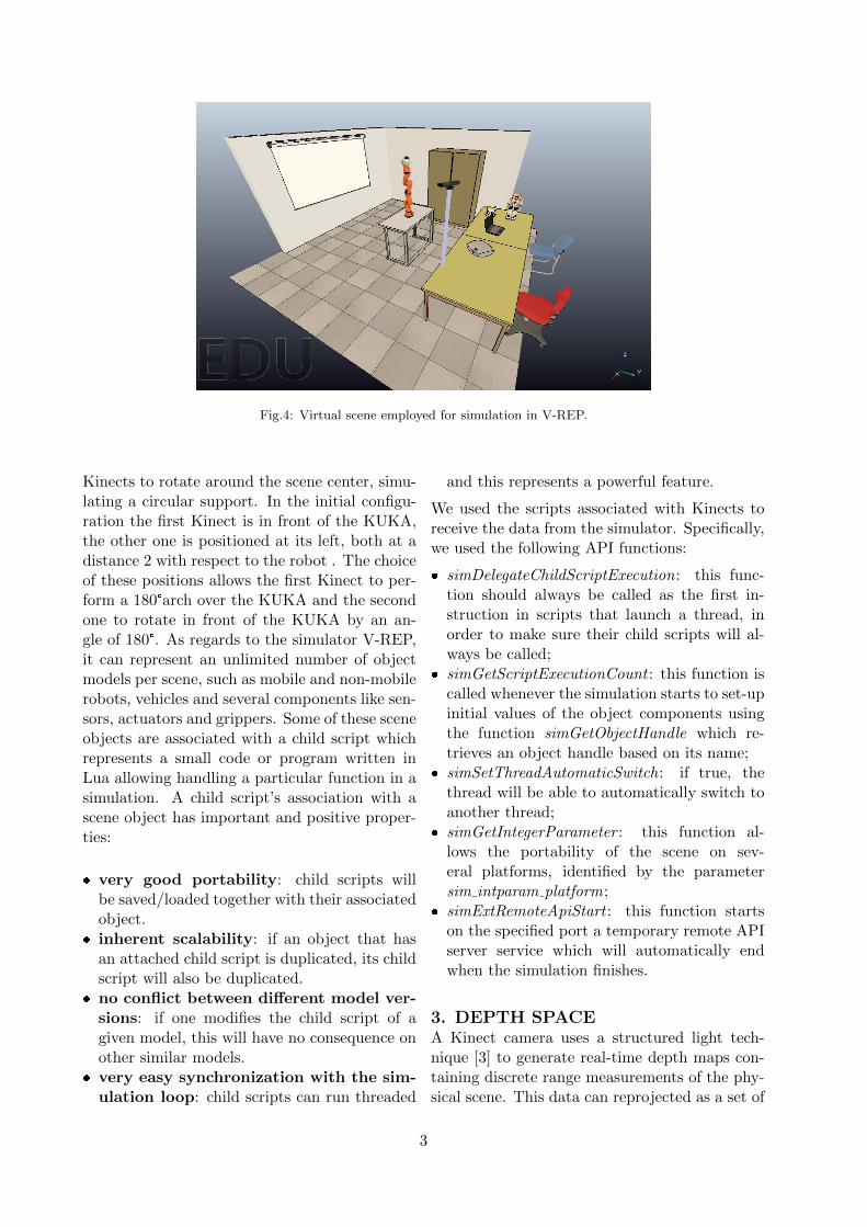
Fig.4: Virtual scene employed for simulation in V-REP.

Kinects to rotate around the scene center, simu-lating a circular support. In the initial configu-ration the first Kinect is in front of the KUKA,the other one is positioned at its left, both at adistance 2 with respect to the robot . The choiceof these positions allows the first Kinect to per-form a 180°arch over the KUKA and the secondone to rotate in front of the KUKA by an an-gle of 180°. As regards to the simulator V-REP,it can represent an unlimited number of objectmodels per scene, such as mobile and non-mobilerobots, vehicles and several components like sen-sors, actuators and grippers. Some of these sceneobjects are associated with a child script whichrepresents a small code or program written inLua allowing handling a particular function in asimulation. A child script’s association with ascene object has important and positive proper-ties:

� very good portability: child scripts willbe saved/loaded together with their associatedobject.

� inherent scalability: if an object that hasan attached child script is duplicated, its childscript will also be duplicated.

� no conflict between different model ver-sions: if one modifies the child script of agiven model, this will have no consequence onother similar models.

� very easy synchronization with the sim-ulation loop: child scripts can run threaded

and this represents a powerful feature.

We used the scripts associated with Kinects toreceive the data from the simulator. Specifically,we used the following API functions:

� simDelegateChildScriptExecution: this func-tion should always be called as the first in-struction in scripts that launch a thread, inorder to make sure their child scripts will al-ways be called;

� simGetScriptExecutionCount : this function iscalled whenever the simulation starts to set-upinitial values of the object components usingthe function simGetObjectHandle which re-trieves an object handle based on its name;

� simSetThreadAutomaticSwitch: if true, thethread will be able to automatically switch toanother thread;

� simGetIntegerParameter : this function al-lows the portability of the scene on sev-eral platforms, identified by the parametersim intparam platform;

� simExtRemoteApiStart : this function startson the specified port a temporary remote APIserver service which will automatically endwhen the simulation finishes.

3. DEPTH SPACEA Kinect camera uses a structured light tech-nique [3] to generate real-time depth maps con-taining discrete range measurements of the phy-sical scene. This data can reprojected as a set of

3

Fig.5: Kinect depth images in V-REP.

discrete 3D points (the so called Point Cloud).To create a complete 3D model, different view-points of the scene must be captured and fusedinto a single representation. For this reasonwe used in this project three Kinects provid-ing three different depth images (see Fig.5) ofthe workspace which can be analyzed as fol-lows. The Depth space is a non-homogenous 212 - dimensional space, where two elements rep-resent the coordinates of the projection of theCartesian point on a plane, and the third ele-ment represents the distance between the pointand the plane. The Kinects that capture thedepth space of the environment can be modeledas a classic pinhole camera. In general, the pin-hole camera model is composed by two sets ofparameters, the intrinsic parameters in cameracalibration matrix K, which model the projec-tion of a Cartesian point on the image plane, andthe extrinsic parameters in matrix E which rep-resents the coordinate transformation betweenthe reference and the sensor frame, i.e.,

K =

fsx 0 cx0 fsy cy0 0 1

and

E =[R|t]

where f is the focal length of the camera, sx andsy are the dimensions of a pixel in meters, cx andcy are the pixel coordinates of the center (on thefocal axis) of the image plane, and R and t arethe rotation and translation between the camera

and the reference frame. Each pixel of a depthimage contains the depth of the observed point,namely the distance between the Cartesian pointand the camera image plane. Note that only thedepth of the closest point along a given ray isstored; all occluded points that are beyond com-pose, for all camera rays, a region of uncertaintyin the Cartesian space called gray area, as shownin Fig.6. Furthermore, the image captured bythe depth sensors contains also points that be-long to the manipulator which instead shouldnot be considered as obstacles. For this reason,the image of the manipulator is removed fromthe depth space and the manipulator does notcontribute to the grey area.

Fig.6: Generation of a depth image, with lighterintensities representing closer objects.

Consider a generic cartesian point expressed inthe reference frame as PR = (xR yR zR)T . Itsexpression in the sensor frame is

PC = (xC yC zC)T = RPR + t

and its projection PD = (px py dp)T in the

depth space is given by

4

px = xcfsxzc

+ cx

py =ycfsyzc

+ cy

dp = zc

where px and py are the pixel coordinates inthe image plane and dp is the depth of thepoint. Once the data obtained from V-REP havebeen transformed, they are inserted in the objectPoint Cloud provided by the Octomap Librarywhich will be described in the next chapter.

4. DATA STRUCTURES AND MAP-PING ALGORITHMS4.1 The OctoMap LibraryThe OctoMap library implements a 3D occu-pancy grid mapping approach and provides datastructures and mapping algorithms. Specifically,the map is implemented in an object of the classOctree and is designed to meet important re-quirements such as:

� Full 3D model. The map is able to model oc-cupied areas and free space which are essentialfor safe robot navigation as well as unknownareas whose information is important, e.g., forautonomous exploration of an environment.

� Updatable. It is possible to add sensor read-ings at any time.

� Flexible. The map extent does not have tobe known in advance: it is multi-resolution sothat, for instance, a high-level planner is ableto use a coarse map, while a local planner mayoperate using a fine resolution.

4.2 The OctoMap Mapping FrameworkThe approach proposed in [4], [5] uses a tree-based representation to offer maximum flexibil-ity with regard to the mapped area and resolu-tion. In our implementation, we created an ob-ject ObstacleModeler which first adds 3 sen-sors, each one associated with a Kinect in V-REP, and then creates two other objects:

� an object DepthSensor for each sensor, thatin turn creates an array of 3D vectors calledqObsCloud which stores, for each sensor, allthe transformed data;

� an object ObstacleSpaceOcTree which usesthe OctoMap library containing data struc-tures and mapping algorithms.

An octree is a hierarchical data structure for spa-tial subdivision in 3D ([6],[7]). In our code, thebasic octree functionality is implemented in theobject map of the class OcTree. Each node inan octree represents the space contained in a cu-bic volume, usually called a voxel. This volumeis recursively subdivided into eight sub-volumesuntil a given minimum voxel size is reached.Fig.7 illustrates an example of an octree stor-ing free (shaded white) and occupied (black)cells. The volumetric model is shown on the leftand the corresponding tree representation on theright.

Fig.7: Example of an octree.

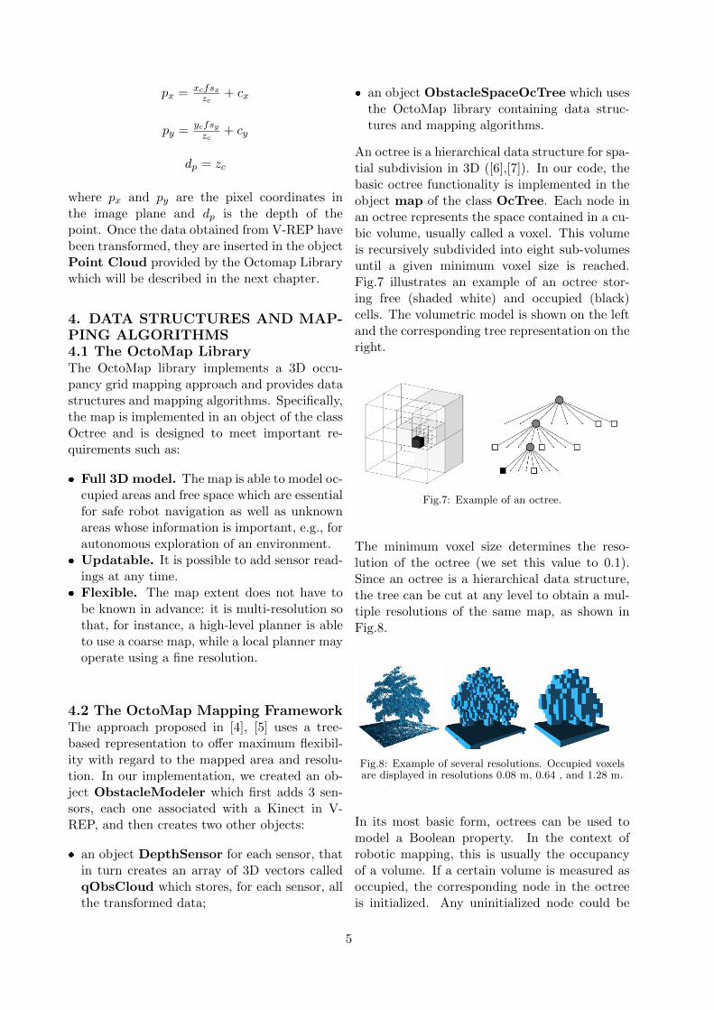
The minimum voxel size determines the reso-lution of the octree (we set this value to 0.1).Since an octree is a hierarchical data structure,the tree can be cut at any level to obtain a mul-tiple resolutions of the same map, as shown inFig.8.

Fig.8: Example of several resolutions. Occupied voxelsare displayed in resolutions 0.08 m, 0.64 , and 1.28 m.

In its most basic form, octrees can be used tomodel a Boolean property. In the context ofrobotic mapping, this is usually the occupancyof a volume. If a certain volume is measured asoccupied, the corresponding node in the octreeis initialized. Any uninitialized node could be

5

free or unknown. To resolve this ambiguity, thefree areas are obtained by clearing the space ona ray from the sensor origin to each measuredend point (see Fig.9).

Fig.9.

In the code, this is done by the functioninsertScan in ObstacleSpaceOcTree whichtakes the data of each DepthSensor object andfor each one calls the function insertPointCloudwhich takes as arguments:

� pointcloud : the measurement of the end-points in the global reference frame;

� sensorPosition: the measurement of theorigin in the global reference frame;

� maxrange: the maximum range of howlong individual beams are inserted.

Thus, we obtain a final map which models all oc-cupied and free cells of the scene. If all childrenof a node in the map have the same state (occu-pied or free) they can be cut using the functionprune. This leads to a substantial reduction inthe number of nodes that need to be maintainedin the tree. To visualize stored octree files and toinspect the data, we used the OpenGL-based 3Dvisualization application octovis available alongwith the library(see Fig.10).

5.OPTIMAL SENSOR PLACEMENT5.1 Gray Area analysisThe Gray Area of a sensor is the set of all Carte-sian points in the scene that are occluded byobstacles. Before detecting cells that belong tothis area, we used the function checkWS to ver-ify that a cell is part of the robot workspacewhich is illustrated in Fig.11.

Fig.11: KUKA Workspace.

Among the occupied and free cells stored inmap we picked only those being in the robotworkspace and put them in the array of 3Dvectors exCubeVector. All the cells of theworkspace which were not in this array are de-fined as ”gray area”.

5.2 Cost functionTo address the problem of optimal placement ofmultiple depth sensors in the environment, weused a probabilistic approach in which we asso-ciate a probability to the cells according withtheir nature. Specifically, we defined two areasin the scene:

Fig.10: The Octree structure with occupied octree volumes (on the left picture) and the occupied (blue) and free(green) volumes (on the right picture).

6

� a probability area: for each cell Ci of thisarea and which is also part of the workspace,we associate an a priori probability P (Ci) =0.5 that there is a human operator.

� an area of interest: for each cell Ci, we asso-ciate a non negative weight w(Ci) = 1 whereasthe cells which are not part of this area have aweight w(Ci) = 0, assigning a larger weight tohe cells we are mainly interested in, accordingwith the task.

The values of probability and weight in these twoareas can be set by the user. Thus, the optimalsensor placement is obtained by minimizing thecost function

J(s) =∑

w(Ci)P (Ci)

where s is the sensor placement containing all thepose parameters of the sensors to be optimized.

6. EXPERIMENTS AND RESULTSIn this chapter we present a solution for threedifferent simulated scenarios. The computationshas been performed on a Intel Core Duo 2.4 GHz.In all the cases taken into account, the simu-lation is performed with a resolution of 0.1 m,rotating the kinects by 180°along a semicirculartrajectory with a 30°scan and decomposing therobot workspace in N = 2572 cubic cells of 10cm side.

Furthermore, we considered as area of interesta cube placed at the center of the scene witha dimension of 8m3 and as probability area aparallelepiped placed in front of the robot at adistance of 1m from its center with dimension12m3.

6.1 Two sensorsIn the first example, shown in Fig.12, we haveconsidered the case of two kinects, the fixed oneplaced at (1, 1.2, 2) and another kinect placed infront of the robot at (0,−2, 1).

Fig.12: Two sensors: initial configuration.

Since the first kinect is fixed, when the otherdepth sensor rotates the result could be incorrectdue to some particular configurations in whichfor example the two sensors are so close (seeFig.13) that we can reconduct to the single sen-sor case.

Fig.13: Two sensors: a particular configuration.

So we expect a large gray area and consequentelya great value of the cost function. In this casethe best solution is obtained in 7 iterations and13 min time for

s∗ = (s∗F , s∗1) = ((1, 1.2, 2), (0,−2, 1)).

6.2 Large gray areaIn the second example we consider the case ofthree kinects, the fixed one placed at (1, 1.2, 2)and the other two kinects in a completely wrongposition, for example behind the wall. In everyconfiguration, we obtained a very large gray areaand the highest value for the cost function J(s).

6.3 Three sensorsIn this last example, we consider three kinects,the fixed one placed at(1, 1.2, 2). This can beconsidered a good compromise between the num-ber of sensors in the scene and a placement close

7

Fig.14: The best solutions for optimal sensor placement.

to optimal. In this case, the gray area is lesswide and we obtained two possible near optimalsolutions (see Fig.14): one for

s∗ = (s∗1, s∗2) = ((2, 0, 1), (0,−1.73, 2))

and another one for

s∗ = (s∗1, s∗2) = ((−2, 0, 1), (0, 1.73, 2))

in both cases with the first kinect parallel to thehorizontal plane and the second one pointing tothe second joint of the robot (30°with respect tohorizontal plane).

7. CONCLUSIONSA procedure to solve the optimal sensor place-ment problem using multiple depth sensors hasbeen proposed. An important aspect is that allthe computations for each sensor are made inparallel and the final data are then merged toobtain a single representation. The optimal sen-sor placement has been formulated using a pro-babilistic approach: after decomposing the scenein cubic cells, the probabilities and weights areassigned to the cells in specific areas of interest,according with the task. These values which canbe set by the user any time allow to compute thefinal cost function, whose minimum value corre-sponds to the best placement for sensors. Re-sults were presented for three different scenarios,highlighting that a wrong placement of the sen-sors does not allow an accurate visualization ofthe working environment.

References

[1] M.Bodor, A.Drenner, P.Schrater, andN.Papanikolopoulos, ”Optimal camera

Placement for automated surveillancetasks,” J. of Intelligent and RoboticSystems, vol.50, pp. 257-295, 2007.

[2] F.Flacco, and A.De Luca, ”MultipleDepth/Presence Sensors: Integration andOptimal Placement for Human/Robot Co-existence,” IEEE International Conferenceon Robotics and Automation, 2010.

[3] B.Freedman, A.Shpunt, M.Machline, andY.Arieli. Depth mapping using projectedpatterns. Patent Application, 10 2008: WO2008/120217 A2.

[4] ”OctoMap: An Efficient Probabilistic 3DMapping Framework Based on Octrees” byA. Hornung, K. M. Wurm, M. Bennewitz,C. Stachniss, and W. Burgard (AutonomousRobots Journal, 2013).

[5] http://octomap.github.io/

[6] Meagher D (1982) Geometric modelingusing octree encoding. Computer Graphicsand Image Processing 19(2):129a147

[7] Wilhelms J, Van Gelder A (1992) Octreesfor faster isosurface generation. ACM TransGraph 11(3):201a227

[8] J.O’Rourke. Art gallery Theorems and Al-gorithms. Oxford University Press. 1987.

[9] D.Lee and A.Lin. Computational complex-ity of art gallery problems. IEEE Trans-actions on Information Theory, 32:276-282,1986.

8