Singularity Avoidance for Over-Actuated, Pseudo-Omnidirectional,

Wheeled Mobile Robots

Christian P. Connette, Christopher Parlitz, Martin Hagele, Alexander Verl

Abstract— For mobile platforms with steerable standardwheels it is necessary to precisely coordinate rotation andsteering angle of their wheels. An established approach toensure this is to represent the current state of motion in formof the Instantaneous Centre of Motion (ICM) and to derivea trajectory within this space. However, while control in theICM space does guarantee adherence to the system’s non-holonomic constraints, it does not avoid the system’s singularconfigurations. Within this work we address the problemof singularity avoidance within the ICM space. Singularitiesrelated to the mathematical representation of the ICM arereduced by a reformulation of this representation. Furthermore,a controller based on artificial potential fields avoiding singularconfigurations of the robot by representing them as obstaclesin the derived ICM space is designed. The resulting controlleris particularized and analyzed w.r.t. the Care-O-bot 3 demon-strator.

I. INTRODUCTION

Mobile service robots operating in domestic environments,

need a high degree of flexibility and agility [1]. Thus, over

the last decades a wide variety of different motion concepts

[2] was investigated. Currently, wheeled platforms appear to

be a promising compromise between a high degree of flexi-

bility, robustness and moderate complexity. The approaches

in this field range from differential driven platforms and

systems with centered or off-centered orientable wheels to

mobile robots that use specially designed wheels [3], [4]. To

balance such requirements against design matters such as a

small footprint and size of the overall system, the mobile

base of the service robot platform Care-O-bot 3 (Fig. 1) was

composed by four orientable standard wheels.

According to the work by Campion, Bastin and D’Andrea-

Novel [5], such a robot has 3 degrees of freedom (DOF)

and these DOFs split into the degree of steerability δs = 2,

associated to the number of independable steerable wheels,

and the degree of mobility δm = 1, associated to the in-

stantaneously accesible velocity space for the planar motion.

Thus, Care-O-bot 3 is a pseudo-omnidirectional mobile robot

able to realize arbitrary velocity and rotational commands,

however only after reorienting its wheels. Furthermore, this

means that all wheels have to be precisely coordinated to

ensure adherence to the system’s non-holonomic constraints.

Besides a variety of different approaches [6], [7], [8],

an often applied strategy to this problem is to control the

robot via its Instantaneous Centre of Motion (ICM) [9],

[10], [11]. However, the ICM-based representation has in

This work was conducted in the department for Robotic Systems at theFraunhofer Institute for Manufacturing Engineering and Automation (IPA),70504 Stuttgart, Germany; Contact: christian.connette@ipa.fraunhofer.de

Fig. 1. Mobile base of Care-O-bot 3, without coating (www.care-o-bot.de)

its standard formulation some numerical drawbacks, which

affect potential control strategies [12]. Also, while control of

the ICM guarantees compliance to the robots nonholonomic

constraints, it does not account for the system’s singularities.

For instance, the control scheme proposed in [12] solves this

problem by constraining the accessible velocity space of the

robot to a region without singular configurations. This need

for the avoidance of singular regions is analogeous to the

problem of obstacle avoidance for mobile robots. Potential

fields [14], [15] have been successfully applied to such global

and local path planning problems [16] and most effective to

local obstacle avoidance problems [17]. Shimoda et. al. [18]

even applied potential fields not only to represent obstacles

but also to express system dynamics in the ”trajectory space”.

Within this work, we address the topic of singularities

related to control of the robot motion via the ICM. We

classify the arising singularities into those resulting from

the mathematical representation of the ICM [13] and those

resulting directly from the system’s kinematics. We shortly

review a method which remedies problems resulting from

the singularities mentioned first by rewriting the ICM as a

spherical coordinate representation of the robots twist ~t =(vx, vy, ω)T. To approach problems arising from the second

type of singularities we propose the usage of a potential field

based controller. We illustrate how singularities in the robot’s

configuration can be expressed as repulsive potentials in the

proposed ICM space. Finally, we particularize the derived

controller with respect to the Care-O-bot 3 demonstrator

(Fig. 1) and analyze it simulative and experimental. At first

however, we give an overview on our system architecture

and the resulting implications for our controller.

2009 IEEE International Conference on Robotics and AutomationKobe International Conference CenterKobe, Japan, May 12-17, 2009

978-1-4244-2789-5/09/$25.00 ©2009 IEEE 4124

xr

yr

yr

zr

h0h1

h2

dw,a

da,i

xa,i

ya,i

φa,i

Fig. 2. Top and front view of Care-O-bot 3’s mobile base

II. SYSTEM OVERVIEW

The platform (Fig. 1 and Fig. 2) has an rectangular

shape with a length of approximately 60 cm and a width of

about 50 cm. The steering-axes of the wheels lie at xa,i =±23,5 cm and ya,i = ±18,5 cm. The wheels are sidewards

off-centered to the steering-axes by dw,a = 2,2 cm. The

chassis clearance h1 is about 5 cm. The total height of the

system h2 is approximately 35 cm.

The control-software of the mobile platform has a multi-

layer structure. Current and velocity control for the actuators

is provided by off-the-shelf motor controllers. The lowest

software-layer comprises the control loop for the robot ve-

locities (vx, vy, ω) generating the set point values (~ωS , ~ωD)for all motor controllers. It provides an interface for higher

level components, for instance, a user interfaces such as a

joypad ( a) in Fig. 3), the navigation module ( b) in Fig. 3)

which closes the position loop or the arm-control module

( c) in Fig. 3) sending velocity requests to the plattform.

Therefore, the velocity control loop has to:

1) ensure adherence to the non-holonomic constraints

a) identify the valid configuration (~ϕS , ~ωD) and

b) derive a valid trajectory (~ϕS , ~ωS , ~ωD, ~ωD)c) respect the actuator limits (~ωS,u, ~ωD,u)

2) approach the commanded velocities fast

3) compensate the steer/drive-coupling (~ωS , ~ωD)

(vx, vy, ω)

ICM based velocity controller

WM1-Ctrl WM2-Ctrl WM3-Ctrl WM4-Ctrl

(~ωS , ~ωD)

a) b) c)

Fig. 3. Schematic of Care-O-bot 3’s software-structure. The ICM basedvelocity controller synchronizes the motion of all wheels. The WMx-Controllers synchronize the steer and drive motors of the single wheelmodules.

xw

yw

xr

yr

ICM

θwr

xwr

ywr

xwICM

ywICM

xrICM

yrICM

ωwr

~vwr

vrx

vry

vwx

vwy

Fig. 4. Applied coordinate systems and ICM

III. ICM SPACE AND SINGULARITIES

A. Classical Definition

There are several corresponding definitions for the In-

stantaneous Centre of Motion (ICM). Within this work, the

ICM is defined as the point in the world coordinate frame,

which instantaneously does not change with respect to the

robot when the latter moving. In Cartesian coordinates, it is

represented as

~xwICM

=

(

xwICM

ywICM

)

=

(

xwr − vw

r,y/ωwr

ywr + vw

r,x/ωwr

)

, (1)

where xwr , yw

r and θwr are components of the robot’s po-

sition and orientation vector ~xwr and vw

r,x, vwr,y, ωw

r are the

components of the robot’s twist ~twr

~xwr =

xwr

ywr

θwr

, ~twr =

vwr,x

vwr,y

ωwr

in the world frame (Fig. 4). Transformation to the robot

coordinate frame delivers

~xrICM

=

(

xrICM

yrICM

)

=

(

−vrr,y/ωr

r

+vrr,x/ωr

r

)

(2)

for the ICM position, where vrr,x, vr

r,y and ωrr are the

components of the robot’s twist ~trr w.r.t the world frame

~trr =

vrr,x

vrr,y

ωrr

=

vwr,x cos(θw

r ) + vwr,y sin(θw

r )−vw

r,x sin(θwr ) + vw

r,y cos(θwr )

ωwr

expressed in the robot coordinate frame. As we are not

interested in the global behavior of the robot we confine our

considerations on the robot-coordinate frame. For a more

convenient writing the indicators of the coordinate system

are omitted. ~tr is written instead of ~trr and ~xICM instead of

~xrICM

respectively.

4125

B. Numerical Issues

The numerical problems arising while using an ICM-based

representation of the twist ~t are twofold. The first problem

is that the transformation fICM(~tr) from the vector represen-

tation of the twist ~tr into the ICM representation (1),(2)

is not injective. Information is lost and the ICM cannot

be transformed back into the twist directly. The second,

more severe problem, is the singularity arising when ωr

becomes zero, leeding to unbounded growth of the controlled

variables.

C. Alternative ICM Representations

These problems have been shown to be reduced if the ICM

is expressed in a form similar to spherical coordinates [13].

The respective transformation equations are

ρICM :=√

v2r,x + v2

r,y + (ωr · dmax)2 (3)

ϕICM := arctan2

(

vr,y

vr,x

)

(4)

θICM := arctan

ωr · dmax√

v2r,x + v2

r,y

(5)

for transforming the twist into the ICM representation.

Where the constant factor dmax renders ωr the same dimen-

sion as the linear velocities. The backwards transformation

is

vr,x = ρICM · cos(θICM) · cos(ϕICM) (6)

vr,y = ρICM · cos(θICM) · sin(ϕICM) (7)

ωr =ρICM

dmax

· sin(θICM) (8)

to transform back from the ICM representation into the

twist ~tr. The evolution of the system configuration is fully

described by the evolution of (ρICM, ϕICM, θICM):

~ϕS = ~f~k1,~k2

(ϕICM, θICM) (9)

~ωS = J~f(ϕICM, θICM) ·

(

ϕICM

θICM

)

(10)

~ωD = ~g~k1,~k2

(ρICM, ϕICM, θICM) (11)

~ωD = J~g(ρICM, ϕICM, θICM) ·

ρICM

ϕICM

θICM

, (12)

where (~k1,~k2) characterize the wheel orientations after

startup. It has to be noted that for pure rotational motion

equation (4) is not defined nor can ϕICM be calculated

by inverting equation (9). In this situation ϕICM is neither

observable nor controllable. However, the associated robot

configuration (~ϕS , ~ωD) and the robot’s rotational rate ωr are

still observable and controllable by (ρICM, θICM) and equations

(8 - 12).

Figures 5 show the critical regions in the ICM rep-

resentation. Figure 5(a) depicts the singularity arising in

the y-component of the ICM if ωr tends towards zeros.

Figures 5(b) to 5(d) depict the critical regions for the

components of the spherical ICM.

-

-

-

-

y-Coordinate of ICM

vx [ms ] ω [ rad

s ]

y [m] 0

00

1

1

2

2

2

2 5

5

(a) Region around Singularity in y-coordinate of ICM

-

-

ρ-Coordinate of ICM

vx [ms ] ω [ rad

s ]

ρ [ms ]

0

00

2

2

2

4

5

5

6

(b) Same region in (vx, ω)-plane for ρ-parameter

-

-

-

θ-Coordinate of ICM

vx [ms ] ω [ rad

s ]

θ [rad] 0

00

1

1

2

2 5

5

(c) θ-parameter: not defined if (vx, vy , ω)T = ~0

-

-

-

ϕ-Coordinate of ICM

vx [ms ] vy [m

s ]

ϕ [rad] 0

00

2

2

2

22

2

(d) ϕ-parameter: not defined for (vx, vy)T = ~0

Fig. 5. Visualization of the critical regions for transformation from velocityto cartesian and spherical ICM space (For Fig. 5(a) - 5(c) vy ≡ 0)

4126

IV. SINGULAR CONFIGURATIONS

In the case of a wheeled mobile robot with orientable

standard wheels, the system degrades if the ICM (xICM, yICM)T

(2) comes near one of the wheel axis (xa,i, ya,i)T , (da,i, φa,i)

(Fig. 2) or

(

ϕa,i

θa,i

)

1,2

=

(

φa,i −π2

arctan(dmax

da,i)

)

,

(

φa,i + π2

− arctan(dmax

da,i)

) (13)

respectively, when expressed in the spherical representation.

For an arbitrary trajectory of the ICM in the (ϕ, θ)-plane

(ϕICM, θICM, ϕICM, θICM), which passes close to but not through

the steering axis of the ith wheel, the necessary steering rate

of the wheel ωS,i grows unbounded as the ICM approaches

the steering axis.

A. Singularities and Actuator Limits

For a given change of the ICM in the cartesian space

(xICM, yICM)T the neccessary steering velocity of the wheels

~ωS depending on the current ICM-position is calculated as

follows:

ωS,i =

√

x2ICM

+ y2ICM

· sin(φ~xICM

− φ~xICM)

√

δx2

ICM,i + δy2

ICM,i

(14)

φ~xICM

= arctan2(yICM, xICM)

φ~xICM= arctan2(δxICM,i, δyICM,i)

(

δxICM,i

δyICM,i

)

=

(

xICM − xa,i

yICM − ya,i

)

Thus, for a given maximum steering rate ωS,max and a given

change of the ICM

∣

∣

∣~xICM

∣

∣

∣, a δmin exists, with

{

~xICM ∈ R2∣

∣

∣

∣

∣

~δICM,i

∣

∣

∣> δmin

}

→ ωS,i < ωS,max. (15)

Vice versa, the critical ICM-positions ~xICM for which (15)

does not hold form a closed circular region around the ithwheel. According to (13) this critical region transforms into

a closed and convex region in the spherical ICM space, as

long as δmin < da,i. Thus, the singularities of the system

can be represented within this ICM space by formulating a

constant repulsive potential.

A worst case approximation of the necessary steering

velocity for the ICM moving in the vicinity of the robot

is depicted in figure 6. The calculations were performed

for a constant absolute change

∣

∣

∣(ϕICM, θICM)T

∣

∣

∣of 1.5π rad/s

for the ICM in its spherical representation. The direction

of the ICM motion was resolved in steps of π/50 rad in

the interval [−π,+π[. Figure 6(a) depicts a chart of the

resulting maximum steering velocity for a single wheel with

the steering axis at xa = 0.235m and ya = 0.185m in the

robot coordinate frame. The according results for the velocity

space in spherical coordinates are depicted in Figure 6(b).

Singular Regions in (x, y)-plane

xICM [m]

y IC

M[m

]

0

0

0.2

-0.2

0.4

-0.4

0.5-0.5

0.6

-0.6

0.8

-0.8

1

1-1-1

(a) Steering velocities with respect to Position of ICM in cart. space

Singular Regions in (ϕ, θ)-plane

ϕICM [rad]

θ IC

M[r

ad]

0

0

0.5

-0.5

1

1

-1

-1

1.5

-1.52-2 3-3

(b) Steering velocities with respect to Position of ICM in spher. space

Fig. 6. Worst case approximation for necessary steering velocity for an ICMmotion with constant absolute speed of 1.5π rad/s. Dark red spaces indicateregions were the necessary steering velocity grows bigger than 8π rad/s,which is the maximum allowed steering rate for a wheel-module.

B. Modeling of the Potential Field

If the necessary steering velocities in the uncritical re-

gions are neglected, the remaining problematic spots have

a roughly convex form which can be approximated by an

ellipsoidal shape. Due to this property we represent them as

repulsive potentials in the well known form

USi =

{

1

2η

(

1

rIS− 1

r0

)2

∀ rIS ≤ r0

0 ∀ rIS ≥ r0

(16)

introduced by Khatib [14], where r0 and η allow to adapt

size and incline of the potential. To adjust the shape of the

repulsive potentials to the form of the critical regions, rIS

was chosen to be an ellipsoidal distance function

r2

IS =(ϕICM − ϕa,i)

2

a2+

(θICM − θa,i)2

b2(17)

with the parameters a and b defining the principal axis of

the ellipse. The resulting force imposed from a singularity

4127

on the ICM is:

FSi =

{

η(

1

rIS− 1

r0

)

1

r3

IS

∂rIS

∂~xICM∀ rIS ≤ r0

0 ∀ rIS ≥ r0

(18)

Analogously, the attracting force is calculated to

FT = −kν(~xICM − ν~xICM,d), (19)

where ~xICM is the current first derivative of the ICM in the

(ϕ, θ)-plane, ~xICM,d is the value, the first derivative of the

ICM would take, if only attracting and frictional forces were

considered

~xICM,d =kp

kν

(xICM,d − xICM), (20)

kp is the proportionality factor between control deviation

and force, kν is the friction coefficient which stabilizes the

controller and ν

ν = min

1,vmax

∣

∣

∣~xICM,d

∣

∣

∣

(21)

ensures that the velocity does not exceed a certain limit. The

variable ρICM - representing the total velocity of the robot -

is controlled independently from the ϕICM and θICM variables

- representing the kinematic configuration of the robot.

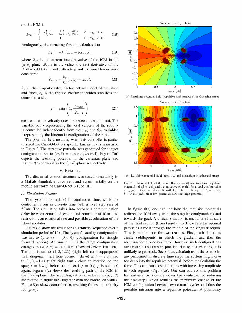
The potential field resulting when this controller is partic-

ularized for Care-O-bot 3’s specific kinematics is visualized

in Figure 7. The attractive potential was generated for a target

configuration set to (ϕ, θ) = (1

2π rad, 2

7π rad). Figure 7(a)

depicts the resulting potential in the cartesian plane and

Figure 7(b) shows it in the (ϕ, θ)-plane respectively.

V. RESULTS

The discussed control structure was tested simulativly in

a Matlab Simulink environment and experimentally on the

mobile plattform of Care-O-bot 3 (Sec. II).

A. Simulation Results

The system is simulated in continuous time, while the

controller is run in discrete time with a fixed step size of

50 ms. The simulation takes into account a communication

delay between controlled system and controller of 10 ms and

restrictions on rotational rate and possible acceleration of the

wheel modules.

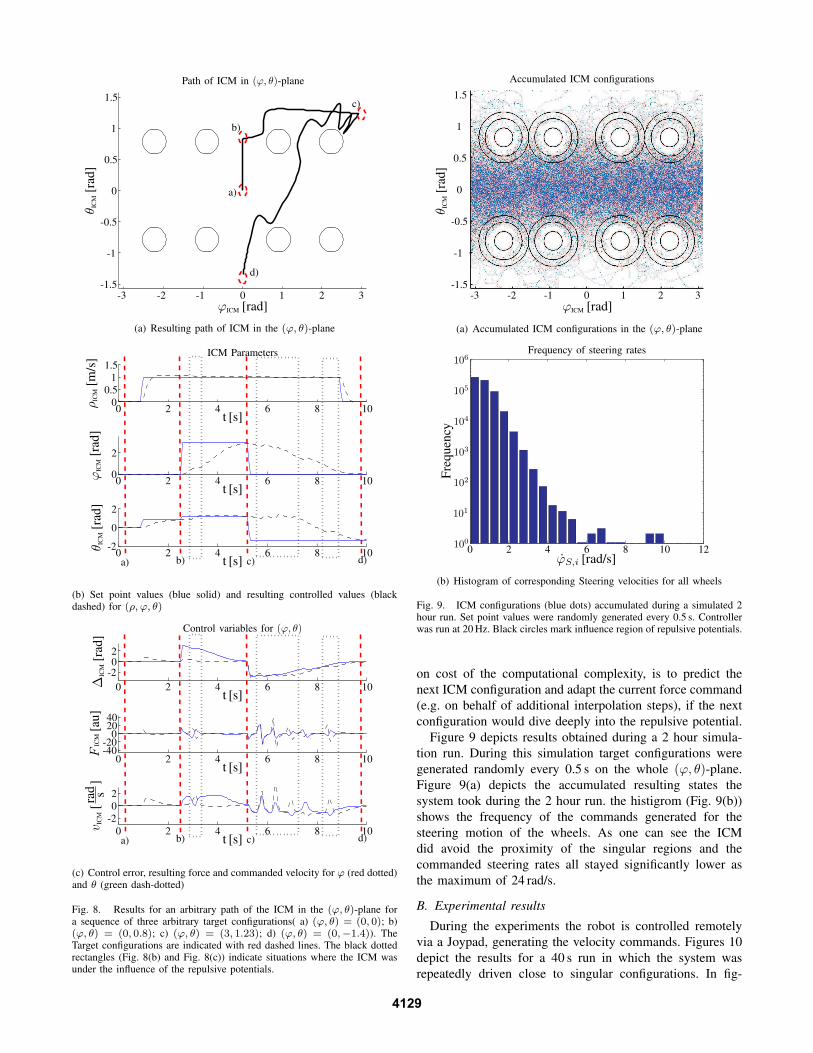
Figures 8 show the result for an arbitrary sequence over a

simulation period of 10 s. The system’s starting configuration

was set to (ρ, ϕ, θ) = (0, 0, 0) (configuration for straight

forward motion). At time t = 1 s the target configuration

changes to (ρ, ϕ, θ) = (1, 0, 0.8) (forward driven left turn).

Then, it is set to (1, 3, 1.23) (tight left turn supperposed

with diagonal - left front corner - drive) at t = 2.6 s and

to (1, 0,−1.4) (tight right turn - close to rotation on the

spot; t = 5.3 s), before at the end (t = 9 s) ρ is set to 0

again. Figure 8(a) shows the resulting path of the ICM in

the (ϕ, θ)-plane. The according set point values for (ρ, ϕ, θ)are plotted in figure 8(b) together with the controlled values.

Figure 8(c) shows control error, resulting forces and velocity

for (ϕ, θ).

Potential in (x, y)-plane

xICM [m]

y IC

M[m

]

0

0

0.2

-0.2

0.4

-0.4

0.5-0.5

0.6

-0.6

0.8

-0.8

1

1-1-1

(a) Resulting potential field (repulsive and attractive) in Cartesian space

Potential in (ϕ, θ)-plane

ϕICM [rad]

θ IC

M[r

ad]

0

0

0.5

-0.5

1

1

-1

-1

1.5

-1.52-2 3-3

(b) Resulting potential field (repulsive and attractive) in spherical space

Fig. 7. Potential field of the controller for (ϕ, θ) resulting from repulsivepotentials of all wheels and the attractive potential for a goal configurationat (ϕ, θ) = ( 1

2π rad, 2

7π rad), with kp = 6, η = 8, r0 = 1.4, a = 0.5,

b = 0.15. (dark blue: low potential; dark red: high potential)

In figure 8(a) one can see how the repulsive potentials

redirect the ICM away from the singular configurations and

towards the goal. A critical situation is encountered at start

of the third section (from target c) to d)), where the optimal

path runs almost through the middle of the singular region.

This is problematic for two reasons. First, such situations

create saddlepoints, in which the gradient and thus the

resulting force becomes zero. However, such configurations

are unstable and thus in practice, due to disturbations, it is

unlikely to get stuck. Second, as calculations of the controller

are performed in discrete time-steps the system might dive

too deep into the repulsive potential, before recalculating the

force. This can cause oscilallations with increasing amplitude

in such regions (Fig. 8(a)). One can address this problem

for instance by slowing down the controller or reducing

the time-steps which reduces the maximum change of the

ICM configuration between two control cycles and thus the

possible intrusion into a repulsive potential. A possibility

4128

Path of ICM in (ϕ, θ)-plane

a)

b)

c)

d)

ϕICM [rad]

θ IC

M[r

ad]

0

0

0.5

-0.5

1

1

-1

-1

1.5

-1.52-2 3-3

(a) Resulting path of ICM in the (ϕ, θ)-plane

a) b) c) d)

ICM Parameters

ρIC

M[m

/s]

ϕIC

M[r

ad]

θ IC

M[r

ad]

t [s]

t [s]

t [s]

0

0

00

00

0.5

1

1.5

2

2

2

2

2

-24

4

4

6

6

6

8

8

8

10

10

10

(b) Set point values (blue solid) and resulting controlled values (blackdashed) for (ρ, ϕ, θ)

a) b) c) d)

Control variables for (ϕ, θ)

∆IC

M[r

ad]

FIC

M[a

u]

v IC

M[ra

d s]

t [s]

t [s]

t [s]

0

0

0

0

0

0

2

2

2

2

2

-2

-2

4

4

4

6

6

6

8

8

8

10

10

10

20

-20

40

-40

(c) Control error, resulting force and commanded velocity for ϕ (red dotted)and θ (green dash-dotted)

Fig. 8. Results for an arbitrary path of the ICM in the (ϕ, θ)-plane fora sequence of three arbitrary target configurations( a) (ϕ, θ) = (0, 0); b)(ϕ, θ) = (0, 0.8); c) (ϕ, θ) = (3, 1.23); d) (ϕ, θ) = (0,−1.4)). TheTarget configurations are indicated with red dashed lines. The black dottedrectangles (Fig. 8(b) and Fig. 8(c)) indicate situations where the ICM wasunder the influence of the repulsive potentials.

ϕICM [rad]

θ IC

M[r

ad]

Accumulated ICM configurations

0

0

0.5

-0.5

1

1

-1

-1

1.5

-1.52-2 3-3

(a) Accumulated ICM configurations in the (ϕ, θ)-plane

ϕS,i [rad/s]

Fre

quen

cy

Frequency of steering rates

0 2 4 6 8 10 12100

101

102

103

104

105

106

(b) Histogram of corresponding Steering velocities for all wheels

Fig. 9. ICM configurations (blue dots) accumulated during a simulated 2hour run. Set point values were randomly generated every 0.5 s. Controllerwas run at 20 Hz. Black circles mark influence region of repulsive potentials.

on cost of the computational complexity, is to predict the

next ICM configuration and adapt the current force command

(e.g. on behalf of additional interpolation steps), if the next

configuration would dive deeply into the repulsive potential.

Figure 9 depicts results obtained during a 2 hour simula-

tion run. During this simulation target configurations were

generated randomly every 0.5 s on the whole (ϕ, θ)-plane.

Figure 9(a) depicts the accumulated resulting states the

system took during the 2 hour run. the histigrom (Fig. 9(b))

shows the frequency of the commands generated for the

steering motion of the wheels. As one can see the ICM

did avoid the proximity of the singular regions and the

commanded steering rates all stayed significantly lower as

the maximum of 24 rad/s.

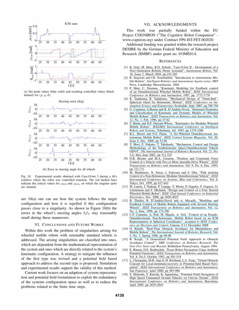
B. Experimental results

During the experiments the robot is controlled remotely

via a Joypad, generating the velocity commands. Figures 10

depict the results for a 40 s run in which the system was

repeatedly driven close to singular configurations. In fig-

4129

ρIC

M[m

/s]

ϕIC

M[r

ad]

θ IC

M[r

ad]

ICM state

t [s]

0

0

0

0.2

0.4

1

-1

5

-5

25

25

25

30

30

30

35

35

35

40

40

40

45

45

45

50

50

50

55

55

55

60

60

60

65

65

65

(a) Set point values (blue solid) and resulting controlled values (blackdashed) for (ρ, ϕ, θ)

t [s]

δϕS

,1δϕ

S,2

δϕS

,3δϕ

S,4

Steering error [deg]

0

0

0

0

10

10

10

10

-10

-10

-10

-10

25

25

25

25

30

30

30

30

35

35

35

35

40

40

40

40

45

45

45

45

50

50

50

50

55

55

55

55

60

60

60

60

65

65

65

65

(b) Error in steering angle for all wheels

Fig. 10. Experimental results obtained with Care-O-bot 3 during a 40 stestdrive where the robot was controlled remotely. The red dashed linesindicate the critical values for ϕICM and ϕICM, on which the singular spotsare situated.

ure 10(a) one can see how the system follows the target

configuration and how it is repelled if this configuration

passes close to a singularity. As shown in Figure 10(b) the

errors in the wheel’s steering angles δ~ϕS stay reasonably

small during these maneuvers.

VI. CONCLUSIONS AND FUTURE WORKS

Within this work the problem of singularities arising for

wheeled mobile robots with orientable standard wheels is

addressed. The arising singularities are classified into ones,

which are dependent from the mathematical representation of

the system and ones which are directly related to the system’s

kinematic configuration. A strategy to mitigate the influence

of the first type was revised and a potential field based

approach to address the second type is proposed. Simulation

and experimental results support the validity of this method.

Current work focuses on an adaption of system representa-

tion and potential field formulation to exploit the redundancy

of the systems configuration space as well as to reduce the

problems related to the finite time steps.

VII. ACKNOWLEDGMENTS

This work was partially funded within the EU

Project COGNIRON (”The Cognitive Robot Companion” -

www.cogniron.org) under Contract FP6-IST-FET-002020.

Additional funding was granted within the research project

DESIRE by the German Federal Ministry of Education and

Research (BMBF) under grant no. 01IME01A

REFERENCES

[1] B. Graf, M. Hans, R.D. Schraft, ”Care-O-bot II - Development of aNext Generation Robotic Home Assistant”, Autonomous Robots, Vol.16, Issue 2, March 2004, pp.193-205

[2] R. Siegwart and I.R. Nourbakhsh, ”Introduction to Autonomous Mo-bile Robots”, Intelligent Robotics and Autonomous Agents series, MITPress, Cambridge Massachusetts, 2004

[3] P. Muir, C. Neuman, ”Kinematic Modeling for Feedback controlof an Omnidirectional Wheeled Mobile Robot”, IEEE International

Conference on Robotics and Automation, 1987, pp. 1772-1778[4] K. Tadakuma, R. Tadakuma, ”Mechanical Design of ”Omni-Ball”:

Spherical wheel for Holonomic Motion”, IEEE Conference on Au-

tomation Science and Engineering, Scottsdale, Sept. 2007, pp.788-794[5] G. Campion, G.Bastin and B. D’Andrea-Novel, ”Structural Properties

and Classification of Kinematic and Dynamic Models of WheeledMobile Robots”, IEEE Transactions on Robotics and Automation, Vol.12, No. 1, Feb. 1996, pp 47-62

[6] T. Burke and H.F. Durrant-Whyte, ”Kinematics for Modular WheeledMobile Robots”, IEEE/RSJ International Conference on Intelligent

Robots and Systems, Yokohama, Jul. 1993, pp 1279-1286[7] K.L. Moore and N.S. Flann, ”A Six-Wheeled Omnidirectional Au-

tonomous Mobile Robot”, IEEE Control Systems Magazine, Vol. 20,Issue 6, Dec. 2000, pp 53-66

[8] Y. Mori, E. Nakano, T. Takahashi, ”Mechanism, Control and DesignMethodology of the Nonholonomic Quasi-Omnidirectional VehicleODV9”, The International Journal of Robotics Research, Vol. 21, No.5-6, May-June 2002, pp 511-525

[9] D.B. Reister and M.A. Unseren, ”Position and Constraint ForceControl of a Vehicle with Two or More steerable Drive Wheels”, IEEE

Transactions on Robotics and Automation, Vol. 9, No. 6, Dec. 1993,pp 723-731

[10] M. Hashimoto, N. Suizu, I. Fujiwara and F. Oba, ”Path trackingControl of a Non-Holonomic Modular Omnidirectional Vehicle”, IEEE

International Conference on Systems, Man and Cybernetics, Vol. 6,Tokyo, Oct. 1999, pp 637-642

[11] M. Lauria, I. Nadeau, P. Lepage, Y. Morin, P. Giguere, F. Gagnon, D.Letourneau and F. Michaud, ”Design and Control of a Four SteeredWheeled Mobile Robot”, IEEE 32nd Annual Conference on Industrial

Electronics, Nov. 2006, pp 4020-4025[12] B. Thuilot, B. D’Andrea-Novel and A. Micaelli, ”Modeling and

Feedback Control of Mobile Robots Equipped with Several SteeringWheels”, IEEE Transactions on Robotics and Automation, Vol. 12,No. 3, June. 1996, pp 375-390

[13] C.P. Connette, A. Pott, M. Hagele, A. Verl, ”Control of an Pseudo-Omnidirectional, Non-holonomic, Mobile Robot based on an ICMRepresentation in Spherical Coordinates”, accepted to IEEE Confer-

ence on Decision and Control, Cancun, 9-11 December 2008[14] O. Khatib, ”Real-Time Obstacle Avoidance for Manipulators and

Mobile Robots”, The International Journal of Robotics Research, Vol.5, No. 1, Spring 1986, pp 90-98

[15] B. Krogh, ”A Generalized Potential Field Approach to ObstacleAvoidance Control”’, SME Conference on Robotics Research: The

Next Five Years and Beyond, Bethlehem Pennsylvania, August 1984[16] E. Rimon, D.E. Koditschek, ”Exact Robot Navigation Using Artificial

Potential Functions”, IEEE Transactions on Robotics and Automation,Vol. 8, No.5, October 1992, pp 501-518

[17] L. Chengqing, M.H. Ang Jr, H. Krishnan, L.S. Yong, ”Virtual ObstacleConcept for Local-minimum-recovery in Potential-field Based Navi-gation”, IEEE International Conference on Robotics and Automation,San Francisco, April 2000, pp 983-988

[18] S. Shimoda, Y. Kuroda, K. Iagnemma, ”Potential Field Navigation ofHigh Speed Unmanned Ground Vehicles on Uneven Terrain”, IEEE

International Conference on Robotics and Automation, Barcelona,April 2005, pp 2839-2844

4130