TU Ilmenau | Universitätsbibliothek | ilmedia, 2020 http://www.tu-ilmenau.de/ilmedia

Zeidis, Igor; Zimmermann, Klaus:

Dynamics of a four-wheeled mobile robot with Mecanum wheels

Original published in: ZAMM : journal of applied mathematics and mechanics. - Weinheim [u.a.]

: Wiley-VCH. - 99 (2019), 12, art. e201900173, 22 pp.

Original published: 2019-11-12

ISSN: 1521-4001 DOI: 10.1002/zamm.201900173 [Visited: 2020-06-08]

This work is licensed under a Creative Commons Attribution 4.0 International license. To view a copy of this license, visit https://creativecommons.org/licenses/by/4.0/

Received: 27 June 2019 Revised: 17 October 2019 Accepted: 26 October 2019

DOI: 10.1002/zamm.201900173

ED ITOR ’ S CHO ICE

Dynamics of a four-wheeled mobile robot with Mecanum wheels

Igor Zeidis Klaus Zimmermann

Department of Mechanical Engineering,

Technische Universität Ilmenau, Thuringia,

Germany

CorrespondenceIgorZeidis,Department ofMechanical Engi-

neering, TechnischeUniversität Ilmenau,

Thuringia,Germany.

Email: igor.zeidis@tu-ilmenau.de

PresentAddressMax-Planck-Ring 12, 98693 Ilmenau,

Germany

Funding informationDeutscheForschungsgemeinschaft,

Grant/AwardNumber: ZI 540-19/2; Euro-

peanSocial Fund,Grant/AwardNumber: 2011

FGR0127

The paper deals with the dynamics of a mobile robot with four Mecanum wheels. For

such a system the kinematical rolling conditions lead to non-holonomic constraints.

From the framework of non-holonomic mechanics Chaplygin’s equation is used to

obtain the exact equation of motion for the robot. Solving the constraint equations for

a part of generalized velocities by using a pseudoinversematrix themechanical system

is transformed to another system that is not equivalent to the original system. Limit-

ing the consideration to certain special types of motions, e.g., translational motion of

the robot or its rotation relative to the center of mass, and impose appropriate con-

straints on the torques applied to the wheels, the solution obtained by means of the

pseudoinverse matrix will coincide with the exact solution. In these cases, the con-

straints imposed on the system become holonomic constraints, which justifies using

Lagrange’s equations of the second kind. Holonomic character of the constraints is a

sufficient condition for applicability of Lagrange’s equations of the second kind but

it is not a necessary condition. Using the methods of non-holonomic mechanics a

greather class of trajectories can be achieved.

KEYWORD SChaplygin’s equation, Mecanum wheels, mobile robots, non-holonomic constraints

1 INTRODUCTION

This paper relates to mechanics of wheeled locomotion. Beside biological inspired forms of locomotion like crawling, flying

or swimming, this form of locomotion with a special propelling device is still in the focus of research. The demand for mobile

platforms working in complex environments or personal robots with a high maneuverability for handicapped people lead to

new kinds of wheels especially in the past fifty years. Starting with the first patent of J. Grabowiecki in 1919 in the U.S.A. [1],

engineers developed wheels which cannot move only in the direction of the wheels plane, but also perpendicular to this plane, e.g.

omnidirectional wheels. A key issue of an efficient application of these wheels and an optimal control of the wholemobile system

is the understanding of the physical interaction between the wheels and the environment. For this reason, mechanics of wheeled

locomotion draws attention of both mechanical engineers, see, e.g., [2–6] and control engineers, e.g., in [7–11]. In a number of

studies e.g. [12–17] the motion of systems with so-called Mecanum wheels, as a special class of omnidirectional wheels, was

investigated. The authors of the mentioned papers mainly use methods of analytical mechanics to obtain the equations of motion.

In many cases the Lagrange equation of second kind is the selected tool, which is correct applicable for holonomic systems.

In this article we consider the classical kinematic constraint, involving point contact and rolling without slipping. There are

more complex models of rolling bodies on the surface, taking into account the contact spot, the distribution of normal pressure

This is an open access article under the terms of the Creative Commons Attribution License, which permits use, distribution and reproduction in any medium, provided the original

work is properly cited.

© 2019 The Authors. ZAMM - Journal of Applied Mathematics and Mechanics Published by Wiley-VCH Verlag GmbH & Co. KGaA

Z Angew Math Mech. 2019;99:e201900173. www.zamm-journal.org 1 of 22https://doi.org/10.1002/zamm.201900173

2 of 22 ZEIDIS AND ZIMMERMANN

F IGURE 1 Four wheeled mobile robot with Mecanum wheels

F IGURE 2 Model of a Mecanum wheel

forces on the contact spot and rolling resistance. Such studies are contained in [18–20], and others. Taking these phenomena

into account is useful in solving a number of practical problems related to the dynamics of Mecanum wheels. The purpose of the

present work was to analyze the method widely used in robotics related to the use of a pseudoinverse matrix and the subsequent

compilation of Lagrange’s equations of the second kind. We called this method approximate. These equations are compared

with equations obtained using non-holonomic mechanics methods. Non-holonomic mechanics methods we called exact.

A Mecanum wheel is a wheel with rollers attached to its circumference. Each roller rotates about an axis that forms an angle

of 45 degrees with the plane of the disk. Such a design provides additional kinematic advantages for the Mecanum wheels in

comparison with the conventional wheels and leads to non-holonomic constraints. Thus, a full non-holonomic approach is used

describing the dynamics of a mobile robot with four Mecanum wheels.

2 FORMULATION OF THE MECHANICAL PROBLEM AND ITSMATHEMATICAL MODEL

The dynamics of a four-wheeled robot with Mecanum wheels arranged on two parallel axles (Figure 1) are studied. The robot

moves so that all its wheels have permanent contact with a plane. The body of the robot has a mass of 𝑚0, its center of mass lies

on the longitudinal axis of symmetry of the body. The distance from the center of mass 𝐶 of the robot to each of its wheel axles

is 𝜌, the distance between the centers of the wheels is 2𝑙. The coordinates of the center of mass in a fixed coordinate system

𝑋𝑂𝑌 are 𝑥𝑐, 𝑦𝑐 , the angle formed by the longitudinal axis of symmetry of the body with axis 𝑂𝑋 is 𝜓 , each wheel has a mass

of 𝑚1. The angles of rotation of the wheels relative to the axes that are perpendicular to the planes of the respective wheels and

pass through their centers are 𝜑𝑖, and the torques applied to the wheels are𝑀𝑖 (𝑖 = 1,… , 4).

2.1 Model of a Mecanum wheelA Mecanum wheel is a wheel with rollers fixed on its outer rim. The axis of each of the rollers forms the same angle 𝛿 (0◦ <𝛿 ≤ 90◦) with the plane of the wheel. As a rule, the angle 𝛿 is equal to 45◦. Each roller may rotate freely about its axis, while the

wheel may roll on the roller. We will model a Mecanum wheel by a thin disk of radius𝑅 ; the velocity 𝑽 𝑃 of the point of contact

𝑃 of the disk with the supporting plane is orthogonal to the axis of the roller, see Figure 2. The rollers are densely attached to the

circumference of the wheel (disk). The dimensions of the rollers are much less than the diameter of the disk and are comparable

ZEIDIS AND ZIMMERMANN 3 of 22

with the disk’s thickness. Within the framework of these assumptions we can use a model of the Mecanum wheel in which the

rollers have infinitesimal dimensions.

Let 𝜸 be the unit vector of the roller’s axis. The wheels move without slip, which implies the constraint

𝑽 𝑃 ⋅ 𝜸 = 0 . (1)

If 𝑽 𝐾 is the velocity of the wheel’s center 𝐾 , then

𝑽 𝑃 = 𝑽 𝐾 + 𝝎 × 𝒓, (2)

where 𝝎 is the angular velocity of the wheel and 𝒓 = ⃖⃖⃖⃖⃖⃖⃗𝐾𝑃 . Let 𝜑 be the angle of rotation of the wheel about the axis that is

perpendicular to the wheel’s plane and passes through its center. Then expression (1) can be represented as follows:

(𝑽 𝐾 −𝑅 �̇� 𝝉) ⋅ 𝜸 = 0 , (3)

where 𝝉 is the unit vector tangent to the wheel’s rim at the point of contact. From expression (3) we find

𝑽 𝐾 ⋅ 𝜸 = 𝑅 �̇� cos 𝛿. (4)

2.2 Kinematic constraint equationsIn what follows, we assume that 𝛿 = 𝜋∕4. Let 𝑽 𝐶 denote the velocity of the center of mass of the mobile robot and let ⃖⃖⃖⃖⃖⃖⃗𝐶𝐾𝑖 = 𝒓𝑖.

Then

𝑽 𝐾𝑖= 𝑽 𝐶 +𝛀 × 𝒓𝑖, 𝑖 = 1,… , 4, (5)

where 𝑽 𝐾𝑖is the velocity of the center of the respective wheel and 𝛀 is the angular velocity of the body of the robot. Then

the kinematic constraint that follows from (4) and represents the condition for rolling without slip along the roller’s axis can be

written as

(𝑽 𝐶 +𝛀 × 𝒓𝑖) ⋅ 𝜸𝑖 =𝑅√2�̇�𝑖, 𝑖 = 1,… , 4. (6)

Here, 𝜸𝑖 is the unit vector that points along the axis of the roller of the respective wheel that has contact with the plane at the

current time instant. Since

(𝛀 × 𝒓𝑖) ⋅ 𝜸𝑖 = (𝒓𝑖 × 𝜸𝑖) ⋅𝛀, 𝑖 = 1,… , 4 (7)

constraint equation (6) can be rewritten as follows:

𝑽 𝐶 ⋅ 𝜸𝑖 + (𝒓𝑖 × 𝜸𝑖) ⋅𝛀 = 𝑅√2�̇�𝑖, 𝑖 = 1,… , 4. (8)

Introduce a robot-attached coordinate system 𝜉𝜂𝜁 with origin at the canter of mass 𝐶 of the cart. We point axis 𝐶𝜉 along the

longitudinal symmetry axis of the cart, axis 𝐶𝜂 along the lateral symmetry axis, and axis 𝐶𝜁 vertically upward. Denote by 𝑉𝐶𝜉and 𝑉𝐶𝜂 the projections of the velocity of the center of mass onto the movable axes 𝐶𝜉 and 𝐶𝜂, respectively, and represent

expression (8) as follows:

𝑉𝐶𝜉𝛾𝑖𝜉 + 𝑉𝐶𝜂𝛾𝑖𝜂 +(𝑟𝑖𝜉𝛾𝑖𝜂 − 𝑟𝑖𝜂𝛾𝑖𝜉)�̇� = 𝑅√2�̇�𝑖,

𝑖 = 1,… , 4.(9)

4 of 22 ZEIDIS AND ZIMMERMANN

Since

𝛾1𝜉 = 𝛾4𝜉 =1√2, 𝛾1𝜂 = 𝛾4𝜂 = − 1√

2,

𝛾2𝜉 = 𝛾3𝜉 =1√2, 𝛾2𝜂 = 𝛾3𝜂 =

1√2,

𝑟1𝜉 = 𝑟2𝜉 = 𝜌, 𝑟1𝜂 = 𝑟3𝜂 = 𝑙,

𝑟3𝜉 = 𝑟4𝜉 = −𝜌, 𝑟2𝜂 = 𝑟4𝜂 = −𝑙

(10)

the constraint equations become

𝑉𝐶𝜉 − 𝑉𝐶𝜂 − (𝜌 + 𝑙)�̇� = 𝑅�̇�1,

𝑉𝐶𝜉 + 𝑉𝐶𝜂 + (𝜌 + 𝑙)�̇� = 𝑅�̇�2,

𝑉𝐶𝜉 + 𝑉𝐶𝜂 − (𝜌 + 𝑙)�̇� = 𝑅�̇�3,

𝑉𝐶𝜉 − 𝑉𝐶𝜂 + (𝜌 + 𝑙)�̇� = 𝑅�̇�4.

(11)

The four Equations (11) can also be represented equivalently in form of the following four equations:

𝑉𝐶𝜉 =𝑅

2(�̇�1 + �̇�2),

𝑉𝐶𝜂 = 𝑅

2(�̇�3 − �̇�1),

�̇� = 𝑅

2(𝜌 + 𝑙)(�̇�2 − �̇�3),

�̇�1 + �̇�2 = �̇�3 + �̇�4.

(12)

The character of constraints is essential for deriving the dynamic equations. If the constraints imposed on a mechanical system

restrict its position, then these constraints are called holonomic (geometrical) constraints. For the systems subject to holonomic

constraints, Lagrange’s equations of the second kind can be used. The constraints that restrict the velocities but do not restrict the

coordinates are called non-holonomic constraints. Such constraints cannot be integrated and reduced to geometrical constraints.

Non-holonomic constraints require different methods for deriving the dynamic equations for the mechanical system. The answer

to the question of whether the system of equations that defines constraints is integrable (holonomic) is given by Frobenius

theorem.[21]

The quantities 𝑉𝐶𝜉 and 𝑉𝐶𝜓 are related to the components �̇�𝑐 and �̇�𝑐 of the velocity vector of the center of mass in the fixed

reference frame by

𝑉𝐶𝜉 = �̇�𝑐 cos𝜓 + �̇�𝑐 sin𝜓,𝑉𝐶𝜂 = −�̇�𝑐 sin𝜓 + �̇�𝑐 cos𝜓.

(13)

Then

�̇�𝑐 = 𝑉𝐶𝜉 cos𝜓 − 𝑉𝐶𝜂 sin𝜓,�̇�𝑐 = 𝑉𝐶𝜉 sin𝜓 + 𝑉𝐶𝜂 cos𝜓.

(14)

Taking into account the first two equations of (12), we can represent (14) as follows:

�̇�𝑐 =𝑅√2cos

(𝜓 − 𝜋

4

)�̇�1 +

𝑅

2(cos𝜓�̇�2 − sin𝜓�̇�3),

�̇�𝑐 =𝑅√2sin

(𝜓 − 𝜋

4

)�̇�1 +

𝑅

2(sin𝜓�̇�2 + cos𝜓�̇�3).

(15)

ZEIDIS AND ZIMMERMANN 5 of 22

The other two equations (12) can be integrated to obtain

𝜓 = 𝑅

2(𝜌 + 𝑙)(𝜑2 − 𝜑3) + 𝐶1,

𝜑4 = 𝜑1 + 𝜑2 − 𝜑3 + 𝐶2,

(16)

where 𝐶1, and 𝐶2 are constants.

Therefore, the system under consideration has two holonomic constraints that allow two generalized coordinates 𝜓 and 𝜑4 to

be eliminated. As to the constraints of (15), they, with reference to (16), can be represented by

�̇�𝑐 = 𝑎1�̇�1 + 𝑎2�̇�2 + 𝑎3�̇�3,

�̇�𝑐 = 𝑏1�̇�1 + 𝑏2�̇�2 + 𝑏3�̇�3.(17)

Here

𝑎1 = 𝑅√2cos

(𝜓 − 𝜋

4

), 𝑏1 =

𝑅√2sin

(𝜓 − 𝜋

4

),

𝑎2 = 𝑅

2cos𝜓, 𝑏2 =

𝑅

2sin𝜓,

𝑎3 = −𝑅

2sin𝜓, 𝑏3 =

𝑅

2cos𝜓.

(18)

The fact that constraints (17) are non-holonomic (non-integrable) implies that not all of the six skew-symmetric quantities

𝛼𝑖𝑗 =𝜕𝑎𝑖

𝜕𝜑𝑗

−𝜕𝑎𝑗

𝜕𝜑𝑖

, 𝛼𝑖𝑗 = −𝛼𝑗𝑖,

𝛽𝑖𝑗 =𝜕𝑏𝑖

𝜕𝜑𝑗

−𝜕𝑏𝑗

𝜕𝜑𝑖

, 𝛽𝑖𝑗 = −𝛽𝑗𝑖,

(𝑖, 𝑗) = (1, 2), (1, 3), (2, 3).

(19)

are equal to zero. For the case under consideration we have

𝛼12 = − 𝑅2

2√2sin

(𝜓 − 𝜋

4

), 𝛼13 =

𝑅2

2√2sin

(𝜓 − 𝜋

4

), 𝛼23 =

𝑅2

2√2sin

(𝜓 + 𝜋

4

),

𝛽12 = 𝑅2

2√2sin

(𝜓 + 𝜋

4

), 𝛽13 = − 𝑅2

2√2sin

(𝜓 + 𝜋

4

), 𝛽23 =

𝑅2

2√2sin

(𝜓 − 𝜋

4

),

(20)

which implies that Equations (15) correspond to non-holonomic constraints.

3 DYNAMIC EQUATIONS OF MOTION OF THE MECHANICAL SYSTEM

Let us assume that the configuration of a mechanical system is defined by 𝑛 generalized coordinates, 𝑞𝑖, 𝑖 = 1,… , 𝑛 of which

𝑛 − 𝑚 coordinates can be expressed in terms of the remaining 𝑚 coordinates by using the non-holonomic constraint equations.

Then the non-holonomic constraint equations can be represented as follows:

�̇�𝑚+𝑘 =𝑚∑𝑠=1

𝑏𝑠,𝑚+𝑘 �̇�𝑠, 𝑘 = 1,… , 𝑛 − 𝑚, (21)

Let the coefficients 𝑏𝑠,𝑚+𝑘 in these equations be functions of only the independent coordinates 𝑞1,… , 𝑞𝑚. Since the constraints

are independent of time (i.e. scleronomic), the kinetic energy of the system is expressed by a quadratic form of the generalized

velocities. Let the coefficients of this quadratic form depend only on the coordinates 𝑞1,… , 𝑞𝑚. Such a mechanical system is

6 of 22 ZEIDIS AND ZIMMERMANN

called Chaplygin system, since they can be described by Chaplygin’s equations for non-holonomic systems. The equations of

motion for such a mechanical system can be represented as follows[22–25]:

𝑑

𝑑𝑡

(𝜕𝑇 ∗

𝜕�̇�𝑠

)− 𝜕𝑇 ∗

𝜕𝑞𝑠+ 𝑃𝑠 = 𝑄𝑠, 𝑠 = 1,… , 𝑚, (22)

where 𝑇 ∗ is the kinetic energy of the system in which the dependent generalized velocities �̇�𝑚+1,… , �̇�𝑛 have been expressed in

terms of the independent velocities �̇�1,… , �̇�𝑚 by using expressions (21), and𝑄𝑠 are the generalized forces. The additional terms

𝑃𝑠 that are accounted by non-holonomic constraints and distinguish these equations from Lagrange’s equations of the second

kind are given by

𝑃𝑠 =𝑛−𝑚∑𝑘=1

𝜕𝑇

𝜕�̇�𝑚+𝑘

𝑚∑𝑟=1

(𝜕𝑏𝑟, 𝑚+𝑘

𝜕𝑞𝑠−𝜕𝑏𝑠, 𝑚+𝑘

𝜕𝑞𝑟

)�̇�𝑟,

𝑠 = 1,… , 𝑚,

(23)

where 𝑇 is the expression for the kinetic energy of the system in which the dependent generalized velocities have not been

expressed in terms of the independent velocities according to (21). Expression (23) implies that the additional terms 𝑃𝑠 vanish

if the constraints are holonomic. In this case,

𝜕𝑏𝑟, 𝑚+𝑘

𝜕𝑞𝑠−𝜕𝑏𝑠, 𝑚+𝑘

𝜕𝑞𝑟= 0 ,

𝑟, 𝑠 = 1,… , 𝑚, 𝑘 = 1,… , 𝑛 − 𝑚.

(24)

However, the terms 𝑃𝑠 may vanish even if the constraints are non-holonomic. In this case, not all of expressions (24) are equal

to zero, but the sum of these expressions multiplied by 𝜕𝑇 ∕𝜕�̇�𝑚+𝑘 vanishes. The respective example is given below.

Chaplygin system allow the dynamic equations of motion to be separated from non-integrable constraint equations,[26] and

therefore, the dynamic equations form a closed system of equation. In addition, these equations have a form of Lagrange’s equa-

tions of the second kind with additional terms due to non-holonomic constraints. These equations are convenient; in particular,

they allow identifying special cases where equations of motion for non-holonomic systems coincide in form with Lagrange’s

equations of the second kind.

The configuration of the system under consideration is defined by seven generalized coordinates: 𝑥𝑐 , 𝑦𝑐 , 𝜓 , 𝜑1, 𝜑2, 𝜑3, 𝜑4.

Since we have four constraint equations, the system has three degrees of freedom. Notice that the coefficients 𝑎𝑖, 𝑏𝑖, 𝑖 = 1,… , 𝑚

in equations of non-holonomic constraints (17) depend only on 𝑚 independent generalized coordinates 𝜑𝑠, 𝑠 = 1,… , 𝑚 (only

on 𝜑2, 𝜑3, in our case) and are independent of 𝑥𝑐 and 𝑦𝑐 . For the mechanical system under consideration, Chaplygin’s equations

are given by

𝑑

𝑑𝑡

(𝜕𝑇 ∗

𝜕�̇�𝑠

)− 𝜕𝑇 ∗

𝜕𝜑𝑠

+ 𝑃𝑠 = 𝑄𝑠, 𝑠 = 1,… , 𝑚,

𝑃𝑠 =𝜕𝑇

𝜕�̇�𝑐

𝑚∑𝑘=1

𝛼𝑘𝑠�̇�𝑘 +𝜕𝑇

𝜕�̇�𝑐

𝑚∑𝑘=1

𝛽𝑘𝑠�̇�𝑘 =𝑚∑𝑘=1

(𝜕𝑇

𝜕�̇�𝑐𝛼𝑘𝑠 +

𝜕𝑇

𝜕�̇�𝑐𝛽𝑘𝑠

)�̇�𝑘.

(25)

Here, 𝑇 ∗ is the function of the kinetic energy of the system from which the velocities 𝑥𝑐 , 𝑦𝑐 have been eliminated using Equa-

tions (17) for non-holonomic constrains, 𝑇 is the kinetic energy of the unconstrained system,𝑄𝑠 are the generalized forces, and

𝑚 is the number of independent generalized coordinates. The additional (as compared with Lagrange’s equations of the second

kind) terms vanish, if all quantities 𝛼𝑘𝑠 and 𝛽𝑘𝑠 are zero, i.e, if the constraints are holonomic. However, as follows from (25), the

terms may vanish also for nonzero 𝛼𝑘𝑠 and 𝛽𝑘𝑠, if the respective sums are equal to zero, i.e., for some cases of non-holonomic

constrains. Then Chaplygin’s equations coincide in form with Lagrange’s equations of the second kind.

To derive the dynamic equations we, first of all, calculate the kinetic energy 𝑇 for the system under consideration. The total

kinetic energy is the sum of the kinetic energy 𝑇0 of the translational motion,

𝑇0 =12(𝑚0 + 4𝑚1)𝑉 2

𝐶(26)

ZEIDIS AND ZIMMERMANN 7 of 22

and the kinetic energy 𝑇1 of the rotational motion,

𝑇1 =12

(𝐽0 + 4

(𝐽2 + 𝑚1(𝜌2 + 𝑙2)

))�̇�2 +

𝐽12(�̇�2

1 + �̇�22 + �̇�2

3 + �̇�24), (27)

where 𝐽0 is the moment of inertia of the body about the center of mass 𝐶 , 𝐽1 is the moment of inertia of the wheel about the

axis that is perpendicular to the plane of the wheel and passes through its center of mass, and 𝐽2 is the moment of inertia of the

wheel about the vertical axis passing through the center of mass of the wheel. Since

𝑉 2𝐶= 𝑉 2

𝐶𝜉+ 𝑉 2

𝐶𝜂= �̇�2𝑐 + �̇�2𝑐 , (28)

the kinetic energy 𝑇 of the mechanical system can be represented as

𝑇 = 12(𝑚𝑠(�̇�2𝑐 + �̇�2𝑐 ) +𝐽𝐶�̇�

2 + 𝐽1(�̇�21 + �̇�2

2 + �̇�23 + �̇�2

4)), (29)

where 𝑚𝑠 = 𝑚0 + 4𝑚1 is the total mass of the mechanical system and 𝐽𝐶 = 𝐽0 + 4(𝐽2 + 𝑚1(𝜌2 + 𝑙2)) is the moment of inertia

of the system about the vertical axis passing through the center of mass.

We will call the equations of motion for deriving which the non-holonomic character of constraints have been taken into

account the exact equations, while the equations derived by another technique that is frequently used in robotics will be called

the approximate equations.

3.1 An approximate technique for deriving the equations of motionIn this section, we will analyze in detail the technique for compiling dynamic equations of a robot with the Mecanum wheels,

which is widely used in robotics.

Consider kinematic constraints (11) as a system of four linear equations for three unknowns, 𝑉𝐶𝜉 , 𝑉𝐶𝜂, and �̇� . This system is

overdetermined and does not have a solution for arbitrary values of �̇�1, �̇�2, �̇�3, and �̇�4. This system may have a solution only if

the equations are linearly dependent. The compatibility condition is given by

�̇�1 + �̇�2 = �̇�3 + �̇�4. (30)

In a number of studies on robotics, e.g., [27–29] the authors, all following and referencing,[14] proceed as follows.

Represent the equations of non-holonomic kinematic constraints (11) in matrix form

�̇� = 𝑱 𝑽 . (31)

Here, vector �̇� has a dimension of 4 × 1, matrix 𝑱 a dimension of 4 × 3, and vector 𝑽 a dimension of 3 × 1

�̇� =

⎛⎜⎜⎜⎜⎜⎝

�̇�1

�̇�2

�̇�3

�̇�4

⎞⎟⎟⎟⎟⎟⎠, 𝑽 =

⎛⎜⎜⎜⎝𝑉𝐶𝜉

𝑉𝐶𝜂

(𝜌 + 𝑙)�̇�

⎞⎟⎟⎟⎠, 𝑱 = 1

𝑅

⎛⎜⎜⎜⎜⎜⎝

1 −1 −11 1 11 1 −11 −1 1

⎞⎟⎟⎟⎟⎟⎠. (32)

Premultiply relation (31) by the transpose 𝑱 𝑇 of the matrix 𝑱 to obtain

𝑱 𝑇 �̇� = 𝑱 𝑇 𝑱 𝑽 . (33)

The 3 × 3 matrix 𝑱 𝑇 𝑱 has the inverse (𝑱 𝑇 𝑱 )−1. Then from (33) we find

𝑽 = 𝑱+�̇�, 𝑱+ = (𝑱 𝑇 𝑱 )−1𝑱 𝑇 . (34)

The 3 × 4 matrix 𝑱+ is called the pseudoinverse of the matrix 𝑱

𝑱+ = 𝑅

4

⎛⎜⎜⎜⎝1 1 1 1

−1 1 1 −1−1 1 −1 1

⎞⎟⎟⎟⎠. (35)

8 of 22 ZEIDIS AND ZIMMERMANN

The values

𝑉𝐶𝜉 =𝑅

4(�̇�1 + �̇�2 + �̇�3 + �̇�4),

𝑉𝐶𝜂 = 𝑅

4(−�̇�1 + �̇�2 + �̇�3 − �̇�4),

�̇� = 𝑅

4(𝜌 + 𝑙)(−�̇�1 + �̇�2 − �̇�3 + �̇�4)

(36)

found in such a way do not satisfy system (31) for arbitrary �̇�1, �̇�2, �̇�3, �̇�4. However, of all possible triples of quantities 𝑉𝐶𝜉 ,

𝑉𝐶𝜂 , �̇� , the triple of (36) provides a minimum for the sum of the squared discrepancies, i.e., the sum of the squared differences

of the left-hand and right-hand sides of the equations of system (31).[30] Of course, if the compatibility relations (30) hold, then

the exact solution of the system of linear equations (11) coincides with the solution constructed by using the pseudoinverse

matrix:

𝑉𝐶𝜉 =𝑅

2(�̇�1 + �̇�2),

𝑉𝐶𝜂 = 𝑅

4(−�̇�1 + �̇�2),

�̇� = 𝑅

2(𝜌 + 𝑙)(�̇�2 − �̇�3).

(37)

Consider then our mechanical system as a system subject to three constrains (36). In this case, the configuration of the system

will be characterized, as previously, by seven generalized coordinates 𝑥𝑐 , 𝑦𝑐 , 𝜓 , 𝜑1, 𝜑2, 𝜑3, and 𝜑4, but now we have three

constraint equations and, hence, the mechanical system has four degrees of freedom. Then the authors of the cited papers use

Lagrange’s equations of the second kind. Setting aside for a while the issue of applicability of Lagrange’s equations of the

second kind to systems with constraints in the form of (36) let us write down these equations. The kinetic energy 𝑇 ∗ obtained

by substituting expressions (36) into (29), taking into account (28), is given by

𝑇 ∗ = 𝐴

2(�̇�21 + �̇�2

2 + �̇�23 + �̇�2

4)− 𝐵(�̇�1�̇�2 − �̇�1�̇�3 − �̇�2�̇�4 + �̇�3�̇�4) + 𝐶(�̇�1�̇�4 + �̇�2�̇�3). (38)

Here

𝐴 =𝑚𝑠𝑅

2

8+

𝐽𝐶𝑅2

16(𝜌 + 𝑙)2+ 𝐽1, 𝐵 =

𝐽𝐶𝑅2

16(𝜌 + 𝑙)2, 𝐶 =

𝑚𝑠𝑅2

8−

𝐽𝐶𝑅2

16(𝜌 + 𝑙)2. (39)

The respective Lagrange’s equations have the form

𝑑

𝑑𝑡

(𝜕𝑇 ∗

𝜕�̇�𝑠

)− 𝜕𝑇 ∗

𝜕𝜑𝑠

= 𝑄𝑠, 𝑠 = 1,… , 4. (40)

Substitute expression (38) for the kinetic energy and into (40) to obtain

𝐴�̈�1 − 𝐵(�̈�2 − �̈�3) + 𝐶�̈�4 = 𝑀1,

𝐴�̈�2 − 𝐵(�̈�1 − �̈�4) + 𝐶�̈�3 = 𝑀2,

𝐴�̈�3 + 𝐵(�̈�1 − �̈�4) + 𝐶�̈�2 = 𝑀3,

𝐴�̈�4 + 𝐵(�̈�2 − �̈�3) + 𝐶�̈�1 = 𝑀4.

(41)

Equations (41) are a system of linear equations for the angular accelerations of rotation of the wheels �̈�𝑠, 𝑠 = 1,… , 4. By solvingthese equations we obtain

�̈�1 = 𝐴1𝑀1 + 𝐵1(𝑀2 −𝑀3) − 𝐶1𝑀4,

�̈�2 = 𝐴1𝑀2 + 𝐵1(𝑀1 −𝑀4) − 𝐶1𝑀3,

�̈�3 = 𝐴1𝑀3 + 𝐵1(𝑀4 −𝑀1) − 𝐶1𝑀2,

�̈�4 = 𝐴1𝑀4 + 𝐵1(𝑀3 −𝑀2) − 𝐶1𝑀1,

(42)

ZEIDIS AND ZIMMERMANN 9 of 22

here

𝐴1 = 𝐴(𝐴 − 𝐶) − 2𝐵2

(𝐴 + 𝐶)(𝐴 − 2𝐵 − 𝐶)(𝐴 + 2𝐵 − 𝐶),

𝐵1 = 𝐵

(𝐴 − 2𝐵 − 𝐶)(𝐴 + 2𝐵 − 𝐶),

𝐶1 = 𝐶(𝐴 − 𝐶) + 2𝐵2

(𝐴 + 𝐶)(𝐴 − 2𝐵 − 𝐶)(𝐴 + 2𝐵 − 𝐶).

(43)

For𝑀𝑠(𝑡), 𝑠 = 1,… , 4 given as a function of time, the system of Equations (42), subject to respective initial conditions, can be

readily integrated. Using the constraint Equations (36), we can find the projections 𝑉𝐶𝜉 , 𝑉𝐶𝜂 of the velocity vector of the center

of mass

𝑉𝐶𝜉 =𝑅

4(𝐴 + 𝐶)

𝑡

∫0

(𝑀1 +𝑀2 +𝑀3 +𝑀4)𝑑𝜏 = 𝑅

4(𝑚𝑅2 + 4𝐽1)

𝑡

∫0

(𝑀1 +𝑀2 +𝑀3 +𝑀4)𝑑𝜏,

𝑉𝐶𝜂 = − 𝑅

4(𝐴 + 𝐶)

𝑡

∫0

(𝑀1 −𝑀2 −𝑀3 +𝑀4)𝑑𝜏 = − 𝑅

𝑚𝑅2 + 4𝐽1

𝑡

∫0

(𝑀1 −𝑀2 −𝑀3 +𝑀4)𝑑𝜏

(44)

and the angular velocity of the body �̇�

�̇� = − 𝑅

4(𝜌 + 𝑙)(𝐴 + 2𝐵 − 𝐶)

𝑡

∫0

(𝑀1 −𝑀2 +𝑀3 −𝑀4)𝑑𝜏 = − 𝑅(𝜌 + 𝑙)𝐽𝐶𝑅

2 + 4𝐽1(𝜌 + 𝑙)2

𝑡

∫0

(𝑀1 −𝑀2 +𝑀3 −𝑀4)𝑑𝜏. (45)

Then, having determined the angle 𝜓 , we can readily find the coordinates 𝑥𝑐 , and 𝑦𝑐 of the center of mass from expressions (14).

Let us revisit the constraint equations (36). Let us have a mechanical system subjected to such constraints. The third equation

can be integrated to obtain the holonomic constraint

𝜓 = 𝑅

4(𝜌 + 𝑙)(−𝜑1 + 𝜑2 − 𝜑3 + 𝜑4) + 𝐶3, (46)

where 𝐶3 is a constant.

Therefore, our system has one holonomic constraint. Using (14), we rewrite the remaining two constraint Equations (36) as

follows:

�̇�𝑐 = 𝑎1�̇�1 + 𝑎2�̇�2 + 𝑎3�̇�3 + 𝑎4�̇�4,

�̇�𝑐 = 𝑏1�̇�1 + 𝑏2�̇�2 + 𝑏3�̇�3 + 𝑏4�̇�4,(47)

where

𝑎1 = 𝑎4 =𝑅

2√2cos

(𝜓 − 𝜋

4

), 𝑎2 = 𝑎3 =

𝑅

2√2cos

(𝜓 + 𝜋

4

),

𝑏1 = 𝑏4 = − 𝑅

2√2cos

(𝜓 + 𝜋

4

), 𝑏2 = 𝑏3 =

𝑅

2√2cos

(𝜓 − 𝜋

4

).

(48)

For this case, non-holonomicity (non-integrability) of constraints (47) implies that some of the twelve skew-symmetric quantities

𝛼𝑖𝑗 =𝜕𝑎𝑖

𝜕𝜑𝑗

−𝜕𝑎𝑗

𝜕𝜑𝑖

, 𝛼𝑖𝑗 = −𝛼𝑗𝑖,

𝛽𝑖𝑗 =𝜕𝑏𝑖

𝜕𝜑𝑗

−𝜕𝑏𝑗

𝜕𝜑𝑖

, 𝛽𝑖𝑗 = −𝛽𝑗𝑖,

(𝑖, 𝑗) = (1, 2), (1, 3), (1, 4), (2, 3), (2, 4), (3, 4).

(49)

10 of 22 ZEIDIS AND ZIMMERMANN

are not equal to zero. In fact,

𝛼12 = 𝛼34 = − 𝑅2

8(𝜌 + 𝑙)sin𝜓, 𝛼13 = 𝛼24 = − 𝑅2

8(𝜌 + 𝑙)cos𝜓,

𝛼14 = − 𝑅2

4√2(𝜌 + 𝑙)

sin(𝜓 − 𝜋

4

), 𝛼23 =

𝑅2

4√2(𝜌 + 𝑙)

sin(𝜓 + 𝜋

4

),

𝛽12 = 𝛽34 =𝑅2

8(𝜌 + 𝑙)cos𝜓, 𝛽13 = 𝛽24 = − 𝑅2

8(𝜌 + 𝑙)sin𝜓,

𝛽14 = 𝑅2

8(𝜌 + 𝑙)sin

(𝜓 + 𝜋

4

), 𝛽23 =

𝑅2

8(𝜌 + 𝑙)sin

(𝜓 − 𝜋

4

).

(50)

Therefore, relations (36) are equations of non-holonomic constraints. The coefficients 𝑎𝑖 and 𝑏𝑖, 𝑖 = 1,… , 4 depend only on

𝜑1, 𝜑2, 𝜑3, 𝜑4 and, hence the system under consideration is a Chaplygin system. The additional terms due to nonholonomic

constraints have the form

𝑃𝑠 =𝜕𝑇

𝜕�̇�𝑐

4∑𝑘=1

𝛼𝑘𝑠�̇�𝑘 +𝜕𝑇

𝜕�̇�𝑐

4∑𝑘=1

𝛽𝑘𝑠�̇�𝑘 =4∑

𝑘=1

(𝜕𝑇

𝜕�̇�𝑐𝛼𝑘𝑠 +

𝜕𝑇

𝜕�̇�𝑐𝛽𝑘𝑠

)�̇�𝑘, (51)

where the kinetic energy 𝑇 is defined by expression (29).

Using relations (50) and (14), we find

𝑃1 =𝑚𝑠𝑅

2

8(𝜌 + 𝑙)

((�̇�𝑐 sin𝜓 − �̇�𝑐 cos𝜓)�̇�2 + (�̇�𝑐 cos𝜓 + �̇�𝑐 sin𝜓)�̇�3 +

√2(�̇�𝑐 sin

(𝜓 − 𝜋

4

)− �̇�𝑐 sin

(𝜓 + 𝜋

4

))�̇�4

)

=𝑚𝑠𝑅

2

8(𝜌 + 𝑙)(−𝑉𝐶𝜂�̇�2 + 𝑉𝐶𝜉�̇�3 − (𝑉𝐶𝜂 + 𝑉𝐶𝜉)�̇�4

).

(52)

Then, using the constraint equations (36) we obtain

𝑃1 =𝑚𝑠𝑅

2

8(𝜌 + 𝑙)⋅𝑅

4(�̇�2 + �̇�3)(�̇�1 − �̇�2 + �̇�3 − �̇�4) = −

𝑚𝑠𝑅2

8(�̇�2 + �̇�3)�̇� . (53)

Similarly,

𝑃2 = 𝑃3 =𝑚𝑠𝑅

2

8(�̇�1 + �̇�4)�̇� , 𝑃4 = 𝑃1. (54)

Finally, the system of dynamic equations, with non-holonomic constraints being taken into account, becomes

𝐴�̈�1 − 𝐵(�̈�2 − �̈�3) + 𝐶�̈�4 − (𝐵 + 𝐶)(�̇�2 + �̇�3)�̇� = 𝑀1,

𝐴�̈�2 − 𝐵(�̈�1 − �̈�4) + 𝐶�̈�3 + (𝐵 + 𝐶)(�̇�1 + �̇�4)�̇� = 𝑀2,

𝐴�̈�3 + 𝐵(�̈�1 − �̈�4) + 𝐶�̈�2 + (𝐵 + 𝐶)(�̇�1 + �̇�4)�̇� = 𝑀3,

𝐴�̈�4 + 𝐵(�̈�2 − �̈�3) + 𝐶�̈�1 − (𝐵 + 𝐶)(�̇�2 + �̇�3)�̇� = 𝑀4.

(55)

Unlike system (41), due to the additional terms, the system of Equations (55) is a set of nonlinear differential equations for the

angular velocities of rotation of the wheels. By solving these equations with respect to the highest derivative we obtain

�̈�1 = 𝑘1(�̇�2 + �̇�3)(−�̇�1 + �̇�2 − �̇�3 + �̇�4) + 𝐴1𝑀1 + 𝐵1(𝑀2 −𝑀3) − 𝐶1𝑀4,

�̈�2 = 𝑘1(�̇�1 + �̇�4)(�̇�1 − �̇�2 + �̇�3 − �̇�4) + 𝐴1𝑀2 + 𝐵1(𝑀1 −𝑀4) − 𝐶1𝑀3,

�̈�3 = 𝑘1(�̇�1 + �̇�4)(�̇�1 − �̇�2 + �̇�3 − �̇�4) + 𝐴1𝑀3 + 𝐵1(𝑀4 −𝑀1) − 𝐶1𝑀2,

�̈�4 = 𝑘1(�̇�2 + �̇�3)(−�̇�1 + �̇�2 − �̇�3 + �̇�4) + 𝐴1𝑀4 + 𝐵1(𝑀3 −𝑀2) − 𝐶1𝑀1,

(56)

ZEIDIS AND ZIMMERMANN 11 of 22

where

𝑘1 =𝑅(𝐵 + 𝐶)

4(𝜌 + 𝑙)(𝐴 + 𝐶). (57)

The angular velocity of rotation of the body �̇� is

�̇� = 𝑅

4(𝜌 + 𝑙)(−�̇�1 + �̇�2 − �̇�3 + �̇�4). (58)

From system (56) it follows that the expression for the angular velocity coincides with expression (45), obtained without taking

into account the non-holonomic nature of the constraints.

Thus, it is shown that if we use the approximate equations of kinematic constraints (36) obtained using the pseudo-inverse

matrix, they still remain non-holonomic and the Lagrange’s equations of the second kind are generally unapplicable to such sys-

tems.

3.2 Exact equations of motion for a non-holonomic systemConsider again the exact system subject to constraints (15) and (16). For this mechanical system, Chaplygin’s equations (25) are

given by

𝑑

𝑑𝑡

(𝜕𝑇 ∗

𝜕�̇�𝑠

)− 𝜕𝑇 ∗

𝜕𝜑𝑠

+ 𝑃𝑠 = 𝑄𝑠, 𝑠 = 1, 2, 3,

𝑃𝑠 =𝜕𝑇

𝜕�̇�𝑐

3∑𝑘=1

𝛼𝑘𝑠�̇�𝑘 +𝜕𝑇

𝜕�̇�𝑐

3∑𝑘=1

𝛽𝑘𝑠�̇�𝑘 =3∑

𝑘=1

(𝜕𝑇

𝜕�̇�𝑐𝛼𝑘𝑠 +

𝜕𝑇

𝜕�̇�𝑐𝛽𝑘𝑠

)�̇�𝑘.

(59)

Calculate the kinetic energy 𝑇 ∗ of the system using expression (29) and constraint equations (11). Since

�̇�2𝑐 + �̇�2𝑐 = 𝑅2

4(2�̇�2

1 + �̇�22 + �̇�2

3 + 2�̇�1�̇�2 − 2�̇�1�̇�3),

�̇�2 = 𝑅2

4(𝜌 + 𝑙)2(�̇�22 + �̇�2

3 − 2�̇�2�̇�3),

(60)

we obtain

𝑇 ∗ = 12

(𝑚𝑠𝑅2

4(2�̇�2

1 + �̇�22 + �̇�2

3 + 2�̇�1�̇�2 − 2�̇�1�̇�3)+ 𝐽1

(2�̇�2

1 + 2�̇�22 + 2�̇�2

3 + 2�̇�1�̇�2 − 2�̇�1�̇�3 − 2�̇�2�̇�3)

+𝐽𝐶𝑅

2

4(𝜌 + 𝑙)2(�̇�21 + �̇�2

3 − 2�̇�2�̇�3))

.

(61)

The additional terms due to nonholonomic constraints are defined by

𝑃1 = −𝑅(𝐵 + 𝐶)(𝜌 + 𝑙)

(�̇�2 + �̇�3)(�̇�2 − �̇�3),

𝑃2 = 𝑅(𝐵 + 𝐶)(𝜌 + 𝑙)

(�̇�1 − �̇�3)(�̇�2 − �̇�3),

𝑃3 = 𝑅(𝐵 + 𝐶)(𝜌 + 𝑙)

(�̇�1 + �̇�2)(�̇�2 − �̇�3).

(62)

Define now the generalized forces 𝑄𝑠, 𝑠 = 1, 2, 3. Using the first expression of (16), we find

𝑄1 = 𝑀1 +𝑀4, 𝑄2 = 𝑀2 +𝑀4, 𝑄3 = 𝑀3 −𝑀4. (63)

12 of 22 ZEIDIS AND ZIMMERMANN

Finally, the dynamic equations become

(𝐴 + 𝐶)(2�̈�1 + �̈�2 − �̈�3) + 𝑃1 = 𝑀1 +𝑀4 ,

(𝐴 + 𝐶)�̈�1 + 2(𝐴 + 𝐵)�̈�2 − (𝐴 + 2𝐵 − 𝐶)�̈�3 + 𝑃2 = 𝑀2 +𝑀4,

−(𝐴 + 𝐶)�̈�1 − (𝐴 + 2𝐵 − 𝐶)�̈�2 + 2(𝐴 + 𝐵)�̈�3 + 𝑃3 = 𝑀3 −𝑀4.

(64)

By solving these equations with respect to the highest derivative we obtain

�̈�1 = 𝑘2(�̇�2 + �̇�3)(�̇�2 − �̇�3) + 𝐴2𝑀1 −(𝐴2 − 𝐶2)

2(𝑀2 −𝑀3) + 𝐶2𝑀4,

�̈�2 = 𝑘2(�̇�3 − 2�̇�1 − �̇�2)(�̇�2 − �̇�3) + 𝐴2𝑀2 −(𝐴2 − 𝐶2)

2(𝑀1 −𝑀4) + 𝐶2𝑀3,

�̈�3 = 𝑘2(�̇�3 − 2�̇�1 − �̇�2)(�̇�2 − �̇�3) + 𝐴2𝑀3 +(𝐴2 − 𝐶2)

2(𝑀1 −𝑀4) + 𝐶2𝑀2,

(65)

here

𝑘2 =𝑅(𝐵 + 𝐶)

2(𝜌 + 𝑙)(𝐴 + 𝐶),

𝐴2 =3𝐴 + 4𝐵 − 𝐶

4(𝐴 + 𝐶)(𝐴 + 2𝐵 − 𝐶), 𝐶2 =

𝐴 + 4𝐵 − 3𝐶4(𝐴 + 𝐶)(𝐴 + 2𝐵 − 𝐶)

.

(66)

For given torques 𝑀𝑖 (𝑖 = 1,… , 4) and initial conditions, we determine the angular velocities �̇�1, �̇�2, �̇�3 by integrating the

system of differential equations (65). Then we use the constraint equations (12) to find

�̇�4 = �̇�1 + �̇�2 − �̇�3,

�̇� = 𝑅

2(𝜌 + 𝑙)(�̇�2 − �̇�3).

(67)

From the system of the Equations (65) follows that expression for �̇� in case of the exact equations coincides with expression

(45) too.

Then we use expressions (15) to calculate the velocities �̇�𝑐 , �̇�𝑐 , and the coordinates of the system’s center of mass 𝐶 .

4 COMPARISON OF THE EXACT AND APPROXIMATE TECHNIQUES

We will find out how the exact and approximate solutions relate to each other. Notice first of all that if the system of dynamic

equations derived by the approximate method is subject to additional compatibility conditions (30) for constraint equations,

then, as mentioned previously, the constraint equations obtained by means of the pseudoinverse matrix coincide with the exact

constraint equations. Since these constraints remain non-holonomic, the exact system of the Equations (64) or (65) should be

compared with the system of the Equations (55) or (56). Relation (30) imposes a constraint on the torques applied to the wheels

(these torques appear on the right-hand side of system (55)):

𝑀1 +𝑀2 = 𝑀3 +𝑀4. (68)

With this constraint, four equations of the systems (55), (56) subject to respective initial conditions are equivalent to three

equations of the systems (64), (65) combined with the relation (30). In fact, by adding the first two equations of the system (55)

and subtracting from the resulting sum the sum of the remaining two equations we obtain

(𝐴 − 2𝐵 − 𝐶)(�̈�1 + �̈�2 − �̈�3 − �̈�4) = 𝑀1 +𝑀2 −𝑀3 −𝑀4, (69)

where 𝐴 − 2𝐵 − 𝐶 = 𝐽1. This implies for the systems (64), (65) that relations (30) hold if and only if (68) holds.

Subject to the condition of (68), the system of dynamic equations (55), (56) with the constraint equations (36) is equivalent

to the system of dynamic equations (64), (65) with the constraint equations (12).

ZEIDIS AND ZIMMERMANN 13 of 22

Compare now the systems of Equations (41) and (64). For these systems to be equivalent, it is required, apart from relation

(68), that the additional terms due to nonholonomic constraints vanish. As follows from Equations (64) this is the case if

�̇�2 − �̇�3 = 0 (70)

or

�̇�1 = −�̇�2 = �̇�3. (71)

For the case (70), as follows from the third relation of (12), the body moves translationally

�̇� = 0, 𝜓 = 𝜓0. (72)

Such a motion subjects the torques to the additional constraints:

𝑀4 = 𝑀1, 𝑀3 = 𝑀2. (73)

Then the system of equations together with the equations of holonomic constraints becomes

(𝐴 + 𝐶)�̈�1 = 𝑀1, (𝐴 + 𝐶)�̈�2 = 𝑀2,

�̇�3 = �̇�2, �̇�4 = �̇�1, 𝜓 = 𝜓0,

�̇�𝑐 =𝑅√2

(cos

(𝜓0 −

𝜋

4

)�̇�1 − sin

(𝜓0 −

𝜋

4

)�̇�2

),

�̇�𝑐 =𝑅√2

(sin

(𝜓0 −

𝜋

4

)�̇�1 + cos

(𝜓0 −

𝜋

4

)�̇�2

).

(74)

where 𝐴 + 𝐶 = 𝑚𝑅2∕4 + 𝐽1.

For the case (71), where �̇�3 = −�̇�2 = �̇�1, the respective motion is a rotation of the body about the center of mass that remains

fixed. In fact, using relations (37) we find that 𝑉𝐶𝜉 = 𝑉𝐶𝜂 = 0, and then from (14) conclude that �̇�𝑐 = �̇�𝑐 = 0 . The additional

constraint for this case is as follows:

𝑀4 = −𝑀3 = 𝑀2 = −𝑀1. (75)

The system of dynamic equations together with the equations of holonomic constraints becomes

(𝐴 + 2𝐵 − 𝐶)�̈�1 = 𝑀1,

�̇�2 = −�̇�1, �̇�3 = �̇�1, �̇�4 = −�̇�1,

�̇� = − 𝑅

𝜌 + 𝑙�̇�1, �̇�𝑐 = �̇�𝑐 = 0.

(76)

where 𝐴 + 2𝐵 − 𝐶 = 𝐽𝐶∕(4(𝜌 + 𝑙)2) + 𝐽1.

As a result, we can draw the following conclusions:

1. If the torques applied to the wheels satisfy relation (68), i.e.,𝑀1 +𝑀2 = 𝑀3 +𝑀4, then for appropriate initial conditions,

the exact system of Equations (64) or (65) is equivalent to the approximate system (55) or (56), where the kinematic relations

are obtained by using the pseudoinverse matrix but the non-holonomic constraints (36) are taken into account.

2. If the torques are subjected to relation (73), i.e.,𝑀4 = 𝑀1,𝑀3 = 𝑀2, (in this case, relation (68) is satisfied automatically),

then the terms accounted for by the non-holonomic constraints disappear, the constraints become holonomic and Lagrange’s

equations of the second kind become applicable. Then the systems of Equations (42) and (56) coincide and are equivalent to the

exact system (65)). In this case, the robot’s body moves translationally (𝜓 = 𝜓0).

3. If the conditions imposed on the torques have the form of (75), then relation (68) again is satisfied automatically, since in

this case,𝑀4 = −𝑀3 = 𝑀2 = −𝑀1. Then the terms accounted for by non-holonomic constraints are absent, and the motion of

the robot is its rotation about the center of mass (�̇�𝑐 = �̇�𝑐 = 0).Let us find out, whether the translational motion of the robot’s body or its rotation about the center of mass are possible for

the exact and approximate models if relation (68) for the torques does not hold and, hence, the exact and approximate systems

of equations are not equivalent to each other.

14 of 22 ZEIDIS AND ZIMMERMANN

For translational motions (�̇� = 0), the terms accounted for by non-holonomic constraints disappear and the approximate

systems of Equations (42) and (56) coincide. For this case, the third kinematic constraint of (36) implies

�̇�1 + �̇�3 = �̇�2 + �̇�4. (77)

Then, from the system of Equations (56) we obtain

(𝐴1 − 2𝐵1 + 𝐶1)(𝑀1 −𝑀2 +𝑀3 −𝑀4) = 0. (78)

Since 𝐴1 − 2𝐵1 + 𝐶1 = 1∕(𝐴 + 2𝐵 − 𝐶) = 1∕(𝐽1 + 𝐽𝐶𝑅2∕(𝜌 + 𝑙)2) ≠ 0, we find

𝑀1 +𝑀3 = 𝑀2 +𝑀4 (79)

In this case, the angular accelerations of the wheels are expressed by

�̈�1 =1

𝐴 + 𝐶

(𝑀1 +

(𝐵 + 𝐶)(𝑀2 −𝑀3)𝐴 − 2𝐵 − 𝐶

),

�̈�2 =(𝐴 − 𝐵)𝑀2 − (𝐵 + 𝐶)𝑀3(𝐴 + 𝐶)(𝐴 − 2𝐵 − 𝐶)

,

�̈�3 =(𝐴 − 𝐵)𝑀3 − (𝐵 + 𝐶)𝑀2(𝐴 + 𝐶)(𝐴 − 2𝐵 − 𝐶)

,

�̈�4 =1

𝐴 + 𝐶

(𝑀1 −

(𝐴 − 𝐵)(𝑀2 −𝑀3)𝐴 − 2𝐵 − 𝐶

).

(80)

In accordance with relations (36), the value of the velocity of the center of mass is defined by

𝑉𝐶𝜉 =𝑅

2(�̇�1 + �̇�3

), 𝑉𝐶𝜂 =

𝑅

2(�̇�2 − �̇�1

). (81)

Solve Equations (80) subject to zero initial conditions to find

𝑉𝐶𝜉 =𝑅

2(𝐴 + 𝐶)

𝑡

∫0

(𝑀1(𝜏) +𝑀3(𝜏)

)𝑑𝜏,

𝑉𝐶𝜂 =𝑅

2(𝐴 + 𝐶)

𝑡

∫0

(𝑀2(𝜏) −𝑀1(𝜏)

)𝑑𝜏.

(82)

We will find a condition, subject to which the system governed by the exact system of Equations (65) moves translationally.

From the third and fourth kinematic relations (12) we find

�̇�3 = �̇�2, �̇�4 = �̇�1. (83)

Then, the system (65) implies the relation

(𝐴2 − 𝐶2)(𝑀1 −𝑀2 +𝑀3 −𝑀4) = 0. (84)

Since 𝐴2 − 𝐶2 = 1∕(2(𝐴 + 2𝐵 − 𝐶)) = 1∕(2𝐽1 + 𝐽𝐶𝑅2∕(2(𝜌 + 𝑙)2)) ≠ 0, the condition for the translational motion of the

robot’s body coincides with relation (79). In this case, since 𝐴2 + 𝐶2 = 𝐴1 − 𝐶1 = 1∕(𝐴 + 𝐶), we obtain

�̈�1 = �̈�4 = 12(𝐴 + 𝐶)

(2𝑀1 −𝑀2 +𝑀3),

�̈�2 = �̈�3 =1

2(𝐴 + 𝐶)(𝑀2 +𝑀3)

(85)

ZEIDIS AND ZIMMERMANN 15 of 22

and the velocity of the center of mass in accordance with relations (12) is expressed by

𝑉𝐶𝜉 =𝑅

2(�̇�1 + �̇�2

), 𝑉𝐶𝜂 =

𝑅

2(�̇�2 − �̇�1

). (86)

Solve Equations (85) subject to zero initial conditions to find the same expression (82).

Thus, the conditions of translational motion for the exact and approximate models coincide. The velocities of the center of

mass and the trajectory of the motion of the center of mass are the same. However, the angular accelerations and the angular

velocities of the wheels are different.

Consider now the rotation of the robot about the center of mass. In this case, �̇�𝑐 = �̇�𝑐 = 0 or 𝑉𝐶𝜉 = 𝑉𝐶𝜂 = 0 , and the terms

accounted for by nonholonomic constraints disappear from the systems of Equations (42) and (56).

For the approximate model, the kinematic relations (36) imply

�̇�2 + �̇�3 = 0, �̇�1 + �̇�4 = 0,

�̇� = 𝑅

2(𝜌 + 𝑙)(�̇�2 − �̇�1).

(87)

Then from the equations of motion (42) we conclude that

𝑀2 +𝑀3 = 0, 𝑀1 +𝑀4 = 0 (88)

and, hence,

�̈�1 = −�̈�4 =(𝐴 − 𝐶)𝑀1 + 2𝐵𝑀2

(𝐴 − 2𝐵 − 𝐶)(𝐴 + 2𝐵 − 𝐶),

�̈�2 = −�̈�3 =2𝐵𝑀1 + (𝐴 − 𝐶)𝑀2

(𝐴 − 2𝐵 − 𝐶)(𝐴 + 2𝐵 − 𝐶).

(89)

The angular velocity of the rotation about the center of mass subject to zero initial conditions is

�̇� = 𝑅

2(𝜌 + 𝑙)(𝐴 + 2𝐵 − 𝐶)

𝑡

∫0

(𝑀2 −𝑀1)𝑑𝜏. (90)

For the exact model, from the kinematic relations (12) we find

�̇�1 = −�̇�2 = �̇�3 = −�̇�4, �̇� = − 𝑅

𝜌 + 𝑙�̇�1 (91)

and, taking into account system (65), we again arrive at relations (88).

For this case,

�̈�1 = −�̈�2 = �̈�3 = −�̈�4 = −𝑀2 −𝑀1

2(𝐴 + 2𝐵 − 𝐶)(92)

and the angular velocity of the rotation of the body about the center of mass coincide with (90).

As it was the case for the translational motion, the conditions for the torques, subject to which the body of the robot rotates

about the center of mass, coincide for the exact and approximate models. However, the angular accelerations of the wheels and

the angular velocity of the rotation of the body about the center of mass are different for these models. Of course, the results of

calculations according to the exact and approximate models coincide if the condition of (30) is imposed.

Therefore, the exact equations coincide with the approximate equations if the torques applied to the wheels satisfy appropriate

relations and the character of the motion is determined in advance.

In the studies on robotics listed previously, only the translational motion of the body, with �̇� = 0 and its rotation about

the center of mass with �̇�𝑐 = �̇�𝑐 = 0, when the angular velocities satisfy the condition, (30) are considered. For these cases, theconstraint equations obtained by means of the pseudoinverse matrix coincide with the exact constraint equations and, in addition,

the constraints become holonomic, which enables Lagrange’s equations of the second kind to be applied.

For these cases, all constraints on the torques presented above are valid. For this reason, the results obtained by using the

pseudoinverse matrix and Lagrange’s equations of the second kind appear to be correct.

16 of 22 ZEIDIS AND ZIMMERMANN

4.1 Calculations according to the exact and approximate modelsConsider a particular case where all torques 𝑀𝑖 (𝑖 = 1,… , 4) applied to the wheels are constant. Let us find the trajectory of

the system for this case on the basis of the approximate model. Solve Equations (44) subject to zero initial conditions to find

𝑉𝐶𝜉 = 𝑀𝜉𝑡, 𝑉𝐶𝜂 = 𝑀𝜂𝑡, �̇� = 𝑀𝜓𝑡, (93)

where

𝑀𝜉 =𝑅

4(𝐴 + 𝐶)(𝑀1 +𝑀2 +𝑀3 +𝑀4),

𝑀𝜂 = − 𝑅

4(𝐴 + 𝐶)(𝑀1 −𝑀2 −𝑀3 +𝑀4),

𝑀𝜓 = − 𝑅

4(𝐴 + 𝐶)(𝐴 + 2𝐵 − 𝐶)(𝑀1 −𝑀2 +𝑀3 −𝑀4).

(94)

Since Equations (93) subject to zero initial conditions imply

𝜓 = 12𝑀𝜓𝑡

2 (95)

from Equations (14) we obtain

�̇�𝑐 = 𝑀𝜉𝑡 cos𝑀𝜓𝑡

2

2−𝑀𝜂𝑡 sin

𝑀𝜓𝑡2

2,

�̇�𝑐 = 𝑀𝜉𝑡 sin𝑀𝜓𝑡

2

2+𝑀𝜂𝑡 cos

𝑀𝜓𝑡2

2.

(96)

Integrating these relations for 𝑥𝑐(0) = 𝑦𝑐(0) = 0 yields

𝑥𝑐 =𝑀𝜉

𝑀𝜓

sin𝑀𝜓𝑡

2

2+

𝑀𝜂

𝑀𝜓

cos𝑀𝜓𝑡

2

2−

𝑀𝜂

𝑀𝜓

,

𝑦𝑐 = −𝑀𝜉

𝑀𝜓

cos𝑀𝜓𝑡

2

2+

𝑀𝜂

𝑀𝜓

sin𝑀𝜓𝑡

2

2+

𝑀𝜉

𝑀𝜓

.

(97)

The trajectory of the center of mass in this case is a circumference

(𝑥𝑐 +

𝑀𝜂

𝑀𝜓

)2+(𝑦𝑐 −

𝑀𝜉

𝑀𝜓

)2=

𝑀2𝜉+𝑀2

𝜂

𝑀2𝜓

. (98)

Therefore, for any constant torques 𝑀𝑖 (𝑖 = 1,… , 4) and zero initial conditions, the trajectory according to the approximate

model is a circumference of radius√

𝑀2𝜉+𝑀2

𝜂 ∕|𝑀𝜓 | centered at the point with coordinates (−𝑀𝜂∕𝑀𝜓,𝑀𝜉∕𝑀𝜓 ). Equa-tion (93) implies

𝑉 2𝐶= 𝑉 2

𝐶𝜉+ 𝑉 2

𝐶𝜂= (𝑀2

𝜉+𝑀2

𝜂 ) 𝑡2, (99)

This means that the center of mass of the system moves along a circumference with a velocity that is increasing in magni-

tude: |𝑉𝐶 | = √𝑀2

𝜉+𝑀2

𝜂 𝑡. The quantity 𝑀𝜉 vanishes if 𝑀1 +𝑀3 = 𝑀2 +𝑀4. In this case, �̇� = 0, and the circumference

degenerates into a straight line

𝑦𝑐 =𝑀𝜂

𝑀𝜉

𝑥𝑐 =𝑀2 −𝑀1𝑀1 +𝑀3

𝑥𝑐. (100)

ZEIDIS AND ZIMMERMANN 17 of 22

F IGURE 3 4WD Arduino compatible Mecanum Robot Kit from

www.robotshop.com (Photo courtesy of RobotShop inc.)

Parameters of the robot for calculations correspond to the prototype shown in Figure 3. The values of the parameters defined

as follows:

𝑚0 = 3.1 𝑘𝑔, 𝑚1 = 0.35 𝑘𝑔, 𝑅 = 0.05𝑚, 𝜌 = 𝑙 = 0.15𝑚,𝐽0 = 0.032 𝑘𝑔𝑚2, 𝐽1 = 6.25 ⋅ 10−4 𝑘𝑔𝑚2, 𝐽2 = 3.13 ⋅ 10−4 𝑘𝑔𝑚2.

(101)

Figures 4–7 plot the computational results for constant all torques𝑀𝑖 (𝑖 = 1,… , 4) and for zero initial conditions.

Figure 4 plots the results of the numerical integration of the nonlinear differential equations that govern the exact nonholo-

nomic model. Let’s set arbitrary constant torques applied to the wheels in the form:

𝑀1 = 0.05Nm, 𝑀2 = 0.25𝑁𝑚, 𝑀3 = −0.05𝑁𝑚, 𝑀4 = 0.20𝑁𝑚. (102)

For arbitrary constant torques applied to the wheels the trajectory of the center of mass is a spiral converging to a focus-type

singular point (Figure 4a). The dependence of coordinates 𝑥𝑐 and 𝑦𝑐 on time 𝑡 is presented on a Figure 4b. On the Figure 4c

are shown dependence of the robot’s rotation angle 𝜓 on time 𝑡, and on a Figure 4d a time dependence of angular velocities of

wheels 𝜔𝑖 (𝑖 = 1,… , 4) on time 𝑡.

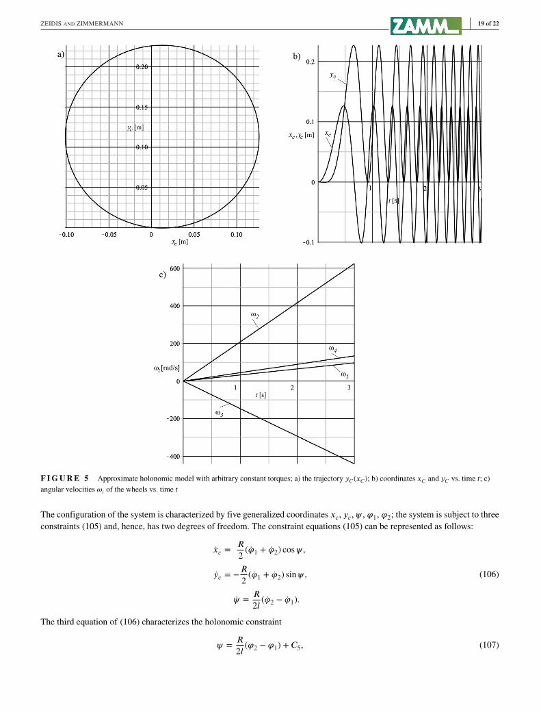
Figure 5 shows the solution of the linear system that corresponds to the approximate model, the nonholonomic constraints

are not being taken into account. For this case, the trajectory of the center of mass for arbitrary constant torques applied to the

wheels (102) is a circumference (Figure 5a). The dependencies of coordinates 𝑥𝑐 and 𝑦𝑐 and angular velocities of wheels 𝜔𝑖

(𝑖 = 1,… , 4) on time 𝑡 are presented on Figures 5b, and 5c, respectively. As it was already noted, the dependence robot’s body

angular rotation 𝜓 on time 𝑡 coincides with Figure 4c.

Figure 6 presents the solution of the system of equations corresponding to the exact model in the case of the translational

motion (𝑀1 +𝑀3 = 𝑀2 +𝑀4). The constant torques applied to the wheels are

𝑀1 = 0.02𝑁𝑚, 𝑀2 = 0.11𝑁𝑚, 𝑀3 = 0.04𝑁𝑚, 𝑀4 = −0.05𝑁𝑚. (103)

For this case, the trajectory of the center of mass is a straight line (Figure 6a). The dependencies angular velocities of wheels 𝜔𝑖

(𝑖 = 1,… , 4) on time 𝑡 are presented on a Figure 6b.

Figure 7 presents the solution of the system of equations corresponding to the exact model in the case of the rotation of the

robot about the center of mass (𝑀2 +𝑀3 = 𝑀1 +𝑀4 = 0). The constant torques applied to the wheels are

𝑀1 = 0.07𝑁𝑚, 𝑀2 = −0.03𝑁𝑚, 𝑀3 = 0.03𝑁𝑚, 𝑀4 = −0.07𝑁𝑚. (104)

In this case the robot rotates about the center of mass. On the Figure 7a are shown dependence of the robot’s body rotation angle

𝜓 on time 𝑡, and on a Figure 7b a time dependence of angular velocities of wheels 𝜔𝑖 (𝑖 = 1,… , 4) on time 𝑡.

The experiments with the prototype, qualitatively confirms the calculations on the basis of the exact nonholonomic model.

5 A REMARK ABOUT LAGRANGE’S EQUATIONS OF THE SECOND KINDAND NON-HOLONOMIC CONSTRAINTS

The holonomic nature of the constraints imposed on a mechanical system is a sufficient condition subject to which Lagrange’s

equation of the second kind can be applied. However, it is not a necessary condition. As has already been mentioned, the

additional terms in Chaplygin’s equations may vanish even if not all coefficients 𝛼𝑠𝑘, 𝛽𝑠𝑘, are equal to zero. In this case, despite

18 of 22 ZEIDIS AND ZIMMERMANN

F IGURE 4 Exact non-holonomic model with arbitrary constant torques; a) the trajectory 𝑦𝐶 (𝑥𝐶 ); b) coordinates 𝑥𝐶 and 𝑦𝐶 vs. time 𝑡; c)

rotation angle 𝜓 vs. time 𝑡; d) angular velocities 𝜔𝑖 of the wheels vs. time 𝑡

the constraints are nonholonomic, equations of motion coincide with Lagrange’s equation of the second kind. Such cases are

known but occur seldom.[31]

As an example, consider the rolling of a wheel pair along a plane. Both wheels are conventional, have the same mass 𝑚1 and

the same radius 𝑅. The wheels are set on the common axle that has a mass of 𝑚0, and a length of 2𝑙 and can freely rotate aboutthis axle. Let 𝑥𝑐 , 𝑦𝑐 be the coordinates of the axle midpoint 𝐶 and let 𝜑1, 𝜑2 denote the angles of rotation of the wheels. The

conditions for this system to roll without slip can be represented as follows[32]:

�̇�𝑐 cos𝜓 + �̇�𝑐 sin𝜓 − 𝑙�̇� = 𝑅�̇�1,

�̇�𝑐 cos𝜓 + �̇�𝑐 sin𝜓 + 𝑙�̇� = 𝑅�̇�2,

−�̇�𝑐 sin𝜓 + �̇�𝑐 cos𝜓 = 0.(105)

ZEIDIS AND ZIMMERMANN 19 of 22

F IGURE 5 Approximate holonomic model with arbitrary constant torques; a) the trajectory 𝑦𝐶 (𝑥𝐶 ); b) coordinates 𝑥𝐶 and 𝑦𝐶 vs. time 𝑡; c)

angular velocities 𝜔𝑖 of the wheels vs. time 𝑡

The configuration of the system is characterized by five generalized coordinates 𝑥𝑐 , 𝑦𝑐 , 𝜓 , 𝜑1, 𝜑2; the system is subject to three

constraints (105) and, hence, has two degrees of freedom. The constraint equations (105) can be represented as follows:

�̇�𝑐 =𝑅

2(�̇�1 + �̇�2) cos𝜓,

�̇�𝑐 = −𝑅

2(�̇�1 + �̇�2) sin𝜓,

�̇� = 𝑅

2𝑙(�̇�2 − �̇�1).

(106)

The third equation of (106) characterizes the holonomic constraint

𝜓 = 𝑅

2𝑙(𝜑2 − 𝜑1) + 𝐶5, (107)

20 of 22 ZEIDIS AND ZIMMERMANN

F IGURE 6 Translational motion with the condition𝑀1 +𝑀3 = 𝑀2 +𝑀4; a) the trajectory 𝑦𝐶 (𝑥𝐶 ); b) angular velocities 𝜔𝑖 of the wheels vs.

time 𝑡

F IGURE 7 Rotational motion about the center of mass with𝑀2 +𝑀3 = 𝑀1 +𝑀4 = 0; a) rotation angle 𝜓 vs. time 𝑡; b) angular velocities 𝜔𝑖

of the wheels vs. time 𝑡

where 𝐶5 is a constant. The kinetic energy 𝑇 of this system is defined by

𝑇 = 12(𝑚𝑠

(�̇�2𝑐 + �̇�2𝑐

)+ 𝐽𝐶�̇�

2 + 𝐽1(�̇�21 + �̇�2

2)), (108)

where 𝑚𝑠 = 𝑚0 + 2𝑚1 is the total mass of the mechanical system, 𝐽𝐶 = 𝐽0 + 2(𝐽2 + 𝑚1𝑙2), and 𝐽0 is the moment of inertia of

the axle about its midpoint, 𝐽1 and 𝐽2 are the moments of inertia of the wheels.

ZEIDIS AND ZIMMERMANN 21 of 22

The quantities

𝛼12 = −𝑅2

4𝑙sin𝜓 = −𝛼21,

𝛽12 = −𝑅2

4𝑙cos𝜓 = −𝛽21

(109)

are not equal to zero and, hence, the first two constraints of (106) are non-holonomic.

However, the additional terms in Chaplygin’s equations vanish. In fact,

𝑃1 = 𝜕𝑇

𝜕�̇�𝑐𝛼21�̇�2 +

𝜕𝑇

𝜕�̇�𝑐𝛽21�̇�2 = 𝑚𝑠(�̇�𝑐𝛼21 + �̇�𝑐𝛽21)�̇�2

=𝑚𝑠𝑅

3

8𝑙(�̇�1 + �̇�2)(cos𝜓 sin𝜓 − sin𝜓 cos𝜓)�̇�2 = 0.

(110)

Similarly, 𝑃2 = 0.Therefore, for the case under consideration, the equations of motion coincide with Lagrange’s equations of the second kind,

although the constraints imposed on the system are non-holonomic.

6 CONCLUSION AND THE FUTURE WORK

The condition subject to which a robot with four Mecanum wheels moves without slip leads to non-holonomic constraints. To

describe the dynamics of such a system one should use equations of motion that are appropriate for mechanical systems with non-

holonomic constraints, for example, Chaplygin’s equations, Voronets’s equations, Appel’s equations, Lagrange’s equations with

multipliers (Lagrange’s equations of the first kind), etc. Lagrange’s equations of the second kind do not apply to non-holonomic

systems in the general case. Apparently, for Chaplygin systems, Chaplygin’s equations should be preferred, since in this case,

the dynamic equations form a closed system with respect to the generalized velocities treated as independent variables. The

holonomic character of the constraints is a sufficient condition for applicability of Lagrange’s equations of the second kind but

it is not a necessary condition. Therefore, the additional terms that distinguish Chaplygin’s equations from Lagrange’s equations

of the second kind may vanish for some systems with non-holonomic constraints. However, such occurrences are rather rare. In

particular, this is not the case for a robot with four Mecanum wheels. In the general case, solving the constraint equations for

a part of the generalized velocities by using the pseudoinverse matrix reduces the mechanical system under consideration to a

system that is not equivalent to the original system, because the number of degrees of freedom of the reduced system is larger

than the number of degrees of freedom of the original system. However, if we confine our consideration to certain special types

of motions, e.g., translational motion of the robot or its rotation relative to the center of mass, and impose appropriate constraints

on the torques applied to the wheels, the solution obtained by means of the pseudoinverse matrix will coincide with the exact

solution. In these cases, the constraints imposed on the system become holonomic constraints, which justifies using Lagrange’s

equations of the second kind. It is just the motions and constraints that are considered in the papers on robotics cited above,

however, it is not stated explicitly. In the general case, the mathematical methods of non-holonomic mechanics should be used.

Subsequent studies are expected to evaluate the effect of the finite linear dimensions of the rollers and the associated

body vibrations.

ACKNOWLEDGEMENT

We would like to thank Prof. N.N. Bolotnik for his critical remarks. We also thank Prof. J. Steigenberger for his permanent

interest in our work. Thank you to Prof. P. Maisser, who showed one of the authors the way to analytical mechanics. This study

was partly supported by the Deutsche Forschungsgemeinschaft (DFG) (project ZI 540-19/2) and by the Development Bank of

Thuringia and the Thuringian Ministry of Economic Affairs with funds of the European Social Fund (ESF) under grant 2011

FGR 0127.

REFERENCES

[1] R. Rojas, A short history of omnidirectional wheels, http://robocup.mi.fu-berlin.de/buch/shortomni.pdf

[2] F. G. Pin, S. M. Killough, A new family of omnidirectional and holonomic wheeled platforms for mobile robots, IEEE Trans. Robot. Autom.1994, 10, 480.

22 of 22 ZEIDIS AND ZIMMERMANN

[3] G. Campion, G. Basin, B. D’Andrea-Novel, Structural properties and classification of kinematic and dynamic models of wheeled mobile robots,

IEEE Trans. Robot. Autom. 1996, 12, 47.[4] M. Wada, S. Mori, Proceedings of the IEEE International Conference on Robotics and Automation, Minneapolis, Minnesota, April, 1996, 1996,

pp. 3671–3676.

[5] J. Ostrowski, J. Burdick, The geometric mechanics of undulatory robotic locomotion, The International Journal of Robotic Research 1998, 17,683.

[6] A. V. Borisov, A. A. Kilin, I. S. Mamaev, An omni-wheel vehicle on a plane and a sphere (in Russian), Rus. J. Nonlin. Dyn. 2011, 7, 785.[7] D. B. Reister, Proceedings of the IEEE International Conference on Robotics and Automation, Sacratmento, California, April, 1991, 1991, pp.

2322–2327.

[8] J. Wu, R. L. Williams, J. Y. Lew, Velocity and acceleration cones for kinematic and dynamic constraints on omni-directional mobile robots,

ASME Transactions on Dynamic Systems, Measurement and Control 2006, 128, 788.[9] K. L. Han, O. K. Choi, I. Lee, S. Choi, Proceedings of the International Conference on Control, Automation and Systems, COEX, Seoul, Oct.

14–17, 2008, 2008, pp. 1290–1295.[10] Y. T.Wang, Y. C. Chen, M. C. Lin, Dynamic object tracking control for a non-holonomic wheeled autonomous robot, Tamkang Journal of Science

and Engineering 2009, 12, 339.[11] C. Stoeger, A.Mueller, H. Gattringer, Parameter identification and model-based control of redundantly actuated, non-holonomic, omnidirectional

vehicles, Informatics in Control, Automation and Robotics. Lecture Notes in Electrical Engineering 2018, 430, 207.[12] P. F. Muir, C. P. Neumann, Kinematic modeling of wheeled mobile robots, J. Robot. Syst. 1987, 4, 281.[13] G. Wampfler, M. Salecker, J. Wittenburg, Kinematics, dynamics, and control of omnidirectional vehicles with mecanum wheels, Mechanics

Based Design of Structures and Machines 1989, 17, 165.[14] P. F. Muir, C. P. Neumann,Kinematic Modeling for Feedback Control of an Omnidirectional Wheeled Mobile Robot, Autonomous Robot Vehicles,

Springer, New York 1990, pp. 25–31.[15] A. Gfrerrer, Geometry and kinematics of the mecanum wheel, Comput.-Aided Geom. Des. 2008, 25, 784.[16] Yu. G. Martynenko, Stability of steady motions of a mobile robot with roller-carrying wheels and a displaced centre of mass, J. Appl. Math.

Mech 2010, 74, 436.[17] M. Abdelrahman, A Contribution to the Development of a Special-Purpose Vehicle for Handicapped Persons - Dynamic Simulations of Mechan-

ical Concepts and the Biomechanical Interaction Between Wheelchair and User, Dissertation Technische Universitaet Ilmenau, Germany 2014.[18] G. Kudra, Awrejcewicz, Approximate modelling of resulting dry friction forces and rolling resistance for elliptic contact shape, Eur. J. Mech. A,

Solids 2013, 42, 358.[19] G. Kudra, Awrejcewicz, Appication and experemental validation of new computational models of friction forces and rolling resistance, Acta

Mech. 2015, 226, 2831.[20] J. Awrejcewicz, G. Kudra, Rolling resistance modelling in the Celtic stone dynamics,Multibody Syst. Dyn. 2019, 45, 155.[21] P. Hartmann, Ordinary Differential Equations, Birkhaeuser, Boston 1982.[22] J. I. Nejmark, N. I. Fufaev, Dynamics of Nonholonomic Systems, American Mathematical Society, Providence 1972.[23] G. Kielau, P. Maisser, Nonholonomic multibody dynamics,Multibody Syst. Dyn. 2003, 9, 213.[24] A. M. Bloch, J. E. Marsden, D. V. Zenkov, Nonholonomic mechanics, Notices of the American Mathematical Society 2005, 52, 320.[25] J. Awrejcewicz, Classical Mechanics - Dynamics, Springer, New York 2012.[26] J. G. Papastavridis, Analytical Mechanics: A Comprehensive Treatise on the Dynamics of Constrained Systems for Engineers, Oxford University

Press, New York 2002.[27] P. Viboonchaicheep, A. Shimada, Y. Kosaka, Industrial Electronics Society, 2003. IECON ’03. The 29th Annual Conference of the IEEE, 2–6

Nov. 2003, 2003, pp. 854–859.[28] M. Killpack, T. Deyle, C. Anderson, C. C. Kemp, Visual Odometry and Control for an Omnidirectional Mobile Robot with a Downward-Facing

Camera, Proc. of IEEE/RSJ International Conference on Intelligent Robots and Systems, Taipei, Taiwan, 18–22 October 2010, IEEE Press,

Piscataway 2010, pp. 139–146.[29] C. Tsai, F. Tai, Y. Lee, Proceedings of the 9th World Congress. Intelligent Control and Automation WCICA, 21–25 June, Taipei, Taiwan 2011,

2011, pp. 546–551.[30] F. R. Gantmacher, The Theory of Matrices, Chelsea Publishing Company, New York 1960.[31] A. S. Sumbatov, Lagrange’s equations in nonholonomic mechanics (in Russian), Russian Journal of Nonlinear Dynamics 2013, 9, 39.[32] K. Zimmermann, I. Zeidis, C. Behn,Mechanics of Terrestrial Locomotion with a Focus on Nonpedal Motion Systems, Springer, Heidelberg 2009.

How to cite this article: I. Zeidis, K. Zimmermann. Dynamics of a four-wheeled mobile robot with Mecanum wheels.

Z Angew Math Mech. 2019;99:e201900173. https://doi.org/10.1002/zamm.201900173