WELL-TO-WHEELS ANALYSIS OF HEAVY-DUTY TRUCK FUELS

A comparison between LNG, LBG and Diesel

SIMON NYLUND

NIKLAS WENSTEDT

School of Business, Society and Engineering Course: Degree project in Energy Engineering Course code: ERA403 Credits: 30hp Program: Masters programme in Sustainable Energy Systems

Supervisor: Esin Iplik, Anna Tisell Examiner: Patrik Klintenberg Customer: Scania CV AB Date: 2019-06-13 Email: snd14002@student.mdh.se nwt14002@student.mdh.se

ABSTRACT

Heavy-duty trucks accounts for 25% CO2 emissions in Sweden and there is approximately 12.6

million heavy-duty vehicles in the EU with different types of fuel and utilization areas. EU is

implementing increased legislations to reduce emissions and increase the use of biofuel and

members of the EU is starting to ban the use of diesel trucks in local areas, which drives the

need to find other suitable fuel. Therefore, to study and compare the emissions and energy

demand in the heavy-duty truck industry a case study is created. Which focuses on production

and processing, transportation, distribution and fuel consumption. Cultivation of maize and

anaerobic digestion of maize, waste and manure is included as well. Data gathered from the

collaboration between the European Commission’s Joint Research Centre, eucar and Concawe

(JEC) is used to create scenarios and these are validated with previous studies. The case study

includes seven LNG cases, three LBG cases and two diesel cases together with several other

cases collected for verification. Furthermore, potential boil-off and leakage during

maintenance is included to further estimate the possible emissions correlated with LNG and

LBG vehicles. The Well-to-Wheels analysis resulted in most LNG and LBG cases having higher

energy input compared to diesel. LBG has the lowest emissions of greenhouse gases. The

transportation method and distance are the most important aspects for the Well-to-Tank

analysis. The fuel consumption is the main source of emissions and energy input in the Tank-

to-Wheels analysis. In conclusion, the transportation and fuel consumption are the greatest

contributors of emissions and energy demand in the complete Well-to-Wheels analysis.

Keywords: Sustainable, energy, GHG, emissions, production, processing, liquefaction,

transportation

PREFACE

This degree project is created as the final part of the Masters programme in energy systems at

Mälardalen University. The work is performed by two students and covers 30hp each in

collaboration with Scania CV AB during the spring of 2019.

We want to thank everyone who participated and contributed to our work and enabled us to

fulfil this degree project. A special appreciation to our supervisors, Anna Tisell at Scania CV

AB and Esin Iplik at Mälardalen University, whom both have been invaluable to this work.

Västerås in June 2019

Simon Nylund

Niklas Wenstedt

SAMMANFATTNING

I Sverige står den tunga lastbilsindustrin för 25 % av koldioxidutsläppen och som en effekt av

klimatförändringarna och miljön i storstäder börjar medlemsländer i EU att förbjuda tunga

lastbilar med diesel som drivmedel i delar av städerna. Vilket har ökat behovet att hitta

substitut till diesel.

I denna studie undersöks därför utsläppen av växthusgaser och energianvändningen från det

att råprodukten tas upp eller odlas fram, renas, omvandlas, transporteras, distribueras och

sedan förbränns i lastbilen. De bränslen som berörs är diesel, flytande naturgas samt flytande

biogas.

Studien är en ”Well-to-Wheels”-analys utformad av flera fallstudier där olika transportvägar,

distribueringssätt, produktionssteg och bränsleförbrukning tillämpas. Totalt har sex scenarion

för flytande naturgas konstruerats, tre för flytande biogas samt ett referensscenario för diesel.

Dessa har använts för jämförelser utifrån data presenterad av JEC. Ytterligare data från andra

studier har verkat som grund för validering av resultaten. Även möjlig ”boil-off” vid

användning av gasbränslena har beräknats och likaså läckage vid underhåll har tagits i

beaktning.

Det som framkom av studien var att flytande naturgas vid lokal produktion och användning

har både lägre energianvändning och utsläpp än diesel. Vid transport av naturgas med

rörledning till en distans av 2500km användes en mindre mängd energi medan utsläppen var

högre än för diesel. Vid likvärdig produktion och transport är diesel mindre energikrävande

och har lägre utsläpp av CO2 ekvivalenter. Produktionen av biogas är den mest energikrävande

av de tre bränslena, medan utsläppen är lägst. Vid biogasproduktion av gödsel och sopor är

utsläppen negativa.

Det har under arbetets gång framkommit att det finns osäkerheter angående värmevärdena

och densiteten för LNG, LBG och diesel, detta tas vidare upp i diskussionen.

Utifrån resultaten konstaterades att transportsätt och distans bränslet färdas innan

förbränning i lastbilen har störst påverkan på utsläpp och energianvändning i ”Well-to-Tank”-

delen. I ”Tank-to-Wheels”-delen av studien är det förbränningen i lastbilen som bidrar till

högst energianvändning och växthusgasutsläpp.

Nyckelord: Hållbar, energi, GHG, utsläpp, produktion, process, förvätskning, transport

CONTENT

1 INTRODUCTION .............................................................................................................1

Background ............................................................................................................. 1

Environment and GWP .................................................................................... 1

Heavy-Duty Truck Industry ............................................................................... 3

Scania .............................................................................................................. 5

Well-To-Wheels ............................................................................................... 5

Liquefied natural gas ........................................................................................ 6

Biogas and Biomethane ................................................................................... 6

Previous research ............................................................................................ 7

Problem statement .................................................................................................. 9

Aim ........................................................................................................................... 9

Research questions ................................................................................................ 9

Delimitation .............................................................................................................10

Contribution to field of study .................................................................................10

2 METHOD ....................................................................................................................... 11

Well-to-tank Cases .................................................................................................12

3 LITERATURE STUDY ................................................................................................... 14

Natural gas characteristics ....................................................................................14

Diesel characteristics .............................................................................................16

Biomass characteristics ........................................................................................17

Fuel production ......................................................................................................18

Production of Natural gas and Crude oil ..........................................................18

Biomass cultivation .........................................................................................20

Production of biogas .......................................................................................21

Processing and purification ...................................................................................26

Biogas upgrading technologies .......................................................................27

Liquefaction process .......................................................................................27

Fuel Transportation ................................................................................................28

Local fuel distribution ............................................................................................29

Fuel consumption ...................................................................................................29

Otto and Diesel engine characteristics ............................................................30

Vehicle emissions ..................................................................................................31

GHG emissions from tail-pipe .........................................................................31

Boil-off gas ......................................................................................................32

Particulate emissions ......................................................................................33

4 WELL-TO-WHEELS ANALYSIS ................................................................................... 35

Well-to-Tank ............................................................................................................35

Biogas production ..................................................................................................35

Biogas production from maize .........................................................................36

Biogas production from waste .........................................................................37

Biogas production from manure ......................................................................37

Liquefaction and upgrading .............................................................................38

Tank-to-Wheels .......................................................................................................38

Boil-off estimations ................................................................................................40

Vehicle maintenance .......................................................................................40

Particulates .............................................................................................................41

Well-to-Wheels ........................................................................................................41

5 RESULTS ...................................................................................................................... 42

Well-to-Tank results ...............................................................................................42

Sensitivity analysis ..........................................................................................45

Tank-to-Wheels results ..........................................................................................47

Energy demand ...............................................................................................47

Greenhouse gas emissions .............................................................................48

Sensitivity analysis Diesel engine efficiency .......................................................49

Boil-off results ........................................................................................................50

Maintenance methane leakage .......................................................................51

Well-to-Wheels results ...........................................................................................52

6 DISCUSSION................................................................................................................. 55

Well-to-Tank discussion ........................................................................................55

Fuel properties ................................................................................................55

Fuel production ...............................................................................................56

Fuel processing ...............................................................................................57

Transportation and distribution ........................................................................57

Tank-to-Wheels discussion ...................................................................................58

Fuel consumption ............................................................................................58

Emissions and particulates .............................................................................59

Boil-off and maintenance ................................................................................60

Well-to-Wheels discussion ....................................................................................61

7 CONCLUSIONS ............................................................................................................ 62

8 SUGGESTIONS FOR FURTHER WORK ...................................................................... 63

Biodiesel .................................................................................................................63

High-pressure direct injection engine ...................................................................63

Origin corresponding to distance .........................................................................63

Economics ..............................................................................................................63

Water footprint ........................................................................................................64

Particulates .............................................................................................................64

Energy input for renewable fuel ............................................................................64

Liquefaction methods ............................................................................................65

9 REFERENCES .............................................................................................................. 66

APPENDIX 1 Previous research used for validation

LIST OF FIGURES

Figure 1 Methane behaviour in the atmosphere. ....................................................................... 2

Figure 2 Well-to-Tank flowchart ................................................................................................ 6

Figure 3 Tank-to-Wheel flowchart ............................................................................................. 6

Figure 4 LNG case visualization ................................................................................................12

Figure 5 LBG case visualization ................................................................................................ 13

Figure 6 Diesel case visualization ............................................................................................. 13

Figure 7 Methane number and Wobbe Index correlation courtesy of EUROMOT. ................. 15

Figure 8 Organic matter decomposition. ..................................................................................21

Figure 9 WTT Energy input for different steps of the cases. ................................................... 43

Figure 10 WTT GHG emissions g CO2eq/MJ .......................................................................... 44

Figure 11 WTT Energy input for different steps of the LBG cases. .......................................... 44

Figure 12 WTT GHG emissions LBG ........................................................................................ 45

Figure 13 Sensitivity analysis of a 10% increase/decrease of the energy input per MJ. .......... 45

Figure 14 Sensitivity analysis of a 10% increase/decrease of emissions in CO2 equivalents per

MJ. ........................................................................................................................... 46

Figure 15 Energy demand as a function of the distance for transportation in the pipeline and

by ship ..................................................................................................................... 46

Figure 16 g CO2eq/MJ as a function of the distance for transportation by pipeline and by ship

................................................................................................................................. 47

Figure 17 TTW emissions of CO2 equivalents per 100km. ...................................................... 48

Figure 18 Pressure build-up in an LNG tank with a heat input of 16.5 and 18 W. .................. 50

Figure 19 Time until an LNG tank is empty with 3 and 4% boil-off. ........................................ 51

Figure 20 Fuel decrease in the tank due to leakage during maintenance. ............................... 51

Figure 21 Complete WTW energy demand in MJ/100 km. ..................................................... 52

Figure 22 Complete WTW pathway emissions in CO2 equivalents per 100 km. .................... 53

Figure 23 WTW GHG emissions for LBG worst case ............................................................... 53

Figure 24 WTW emissions per 100km in percentage including a boil-off rate of 4% and

maintenance for GWP100. ........................................................................................ 54

Figure 25 WTW emissions per 100km in percentage including a boil-off rate of 4% and

maintenance for GWP20. ........................................................................................ 54

LIST OF TABLES

Table 1 Difference in heating values on weight and volume basis. ...........................................16

Table 2 Emissions and energy demand values for oil and natural gas production. .................19

Table 3 Methane yield per tonne volatile solids (VS) .............................................................. 20

Table 4 CO2eq emissions using different methods and substrates ......................................... 23

Table 5 Manure, Organic waste and Maize CO2 emissions ..................................................... 24

Table 6 Direct energy input for biogas production (MJ/MJ biogas) using the ISO-method .. 24

Table 7 GHG emissions from biogas production using the ISO-method ................................ 25

Table 8 Gas yield and energy demand for organic waste and manure .................................... 25

Table 9 Effect of manure usage for biogas production in Sweden ........................................... 26

Table 10 Net effects on emissions from biogas production (per Nm3 methane) .................... 26

Table 11 Global Warming Potential Values for CH4 and N2O .................................................. 31

Table 12 Euro VI Heavy-duty regulations. ............................................................................... 32

Table 13 Emissions from the reference vehicles. ..................................................................... 32

Table 14 CO2 emission factors for LNG and Diesel ................................................................. 32

Table 15 General biogas and methane data.............................................................................. 36

Table 16 Biogas potential from maize - Data ........................................................................... 36

Table 17 Data for TTW calculations used ................................................................................. 39

Table 18 Reference vehicle properties ..................................................................................... 40

Table 19 WTT scenarios LNG and LBG .................................................................................... 42

Table 20 LNG TTW energy result ............................................................................................ 47

Table 21 Diesel TTW energy result........................................................................................... 48

Table 22 Values used for TTW GHG emissions ....................................................................... 48

Table 23 Emissions per 100km for the reference vehicles. ...................................................... 49

Table 24 Diesel efficiency sensitivity analysis for GHG emissions .......................................... 49

Table 25 Diesel efficiency sensitivity analysis for energy demand .......................................... 50

Table 26 Methane leakage during maintenance. ...................................................................... 51

NOMENCLATURE

Symbol Description Unit

F heat value of fuel MJ/kg

P Power W

FC Fuel consumption Kg/100km

ABBREVIATIONS

Abbreviation Description

AD Anaerobic digestion

BOG Boil-off gas

CF Conformity factors

CNG Compressed Natural Gas

CO2eq Carbon dioxide equivalent

DS Dry solids

GHG Greenhouse gases

GTW Gross Trailer Weight

GWP Global Warming Potential

HP High pressure

LBG Liquefied Biogas

LHV Lower Heating Value

LNG Liquefied Natural Gas

PEMS Portable Emission Measuring System

PES Primary Energy Source

PM Particulate matter

PN Particulate number

SCR Selective catalytic reduction

THC Total Hydrocarbons

TTW Tank-to-Wheels

VECTO Vehicle Energy Calculation Tool

WHTC World Harmonized Vehicle Cycle

VS Volatile solids

WTT Well-to-Tank

WTW Well-to-Wheels

DEFINITIONS

Definition Description

Boil-off Methane released from the tank due to high pressure

Slip Unburned methane in the exhaust

1

1 INTRODUCTION

Long haulage transportation of goods is a continuously growing market and the main fuels

today are fossil fuels such as diesel. Due to the increase of the average global temperature, the

release of greenhouse gases is a growing topic. Many larger cities in Europe have now limited

the use of older diesel vehicles due to the particles released which increases the need of a

complimentary fuel as well.

This degree project is a case study concerning the emissions from natural gas, diesel and

biogas. It is presented in a Well-to-Wheels analysis to determine if biogas or natural gas in

liquid form is a more environmentally friendly fuel than diesel. In this introductory section the

background of the study concerning the different emissions and the transportation industry is

presented and followed by the aim of this work.

This degree project is conducted on behalf of Scania due to the increased demand of vehicles

that are using natural gas (NG) specifically liquefied natural gas (LNG), as fuel. Therefore, the

environmental impact of LNG compared to diesel is of interest for a company with a

commitment to reduce emissions.

Background

Relevant data to understand the research questions and the aim is described in the following

section. The headlines are divided into the environmental impact, the heavy-duty truck and

vehicle as well as theory of Well-to-Wheels analysis. Previous research within the area of work

is presented for further understanding on the topic.

Environment and GWP

According to Stattin (2012) the global average temperature has increased since the

preindustrial level by 0.7 °C due to an increased use of fossil fuels. When the fuels are

combusted, greenhouse gases are emitted to the atmosphere which absorbs some of the energy

returning to space from Earth. Without the greenhouse gases Earth would have an average

temperature of close to -18 °C (due to the geothermal energy from Earth and the solar

radiation). With the greenhouse gases, nitrogen, oxygen and water vapour this temperature

should be +15 °C.

Natowitz and Ngô (2009) state that water vapour accounts for 55% of the natural greenhouse

effect and CO2 accounts for 39%. Other greenhouse gases are methane (CH4), nitrous oxide

(N2O), Ozone (O3) and halocarbons. These figures are not the global concentration in the

atmosphere but an order of magnitude in the greenhouse effect aspect. The global

2

concentration in the atmosphere for CO2 is currently 400 ppmv (parts per million by volume)

which is an increase from the 280 ppmv measured in the preindustrial period. An even bigger

percentile increase has been measured for the concentration of CH4, which had a value of 580

to 783 ppb (parts per billion) pre-industrialization and has a current concentration of 2000

ppb.

Natowitz and Ngô (2009) claim that a large part of the anthropogenic greenhouse gas

emissions is due to energy generation, of which CO2 emissions are dominant. This is because

80% of our primary fuel is fossil based (oil, coal, natural gas). Noteworthy is that a quarter of

the emissions globally come from the transportation sector.

According to Reay (2007) the effect of methane in the atmosphere is divided, because the

composition of the gas is changing in the atmosphere together with other gases. This affects

the lifetime of methane which makes it hard to estimate the CO2 equivalence. The CH4 can be

destroyed by ultra violet (UV) rays under free radical halogenation (March, 2007). The

dominant issue with methane is the mechanism oxidation by OH, which can lead to the

formation of ozone and thereby affect the oxidizing capacity of the atmosphere according to

the following expression.

𝐶𝐻4 + 𝑂𝐻 → 𝐶𝐻3 +𝐻2𝑂 → ⋯𝐶𝑂 + 𝑃𝑟𝑜𝑑𝑢𝑐𝑡𝑠… → 𝐶𝑂2 + 𝑃𝑟𝑜𝑑𝑢𝑐𝑡𝑠

The formula is illustrated by Pandis & Seinfeld (1998) in Figure 1.

Figure 1 Methane behaviour in the atmosphere.

The chemical formula is simplified due to the many steps involved. There is also the possibility

that CH4 reacts with Cl according to the following formula.

3

𝐶𝑙 + 𝐶𝐻4 → 𝐻𝐶𝑙+ 𝐶𝐻3

Methane is estimated by Stattin (2012) to have an average lifetime of 10-15 years in the

atmosphere. From an environmental perspective, combustion of methane is considered as a

“clean” fuel, when CO2 emissions are concerned.

To be able to estimate the greenhouse effect from different gases a greenhouse warming

potential (GWP) has been defined as “the cumulative radiative forcing from the emission of a

unit mass of gas relative to a reference gas” (Natowitz and Ngô, 2009, p.103). Natowitz and

Ngô (2009) states that the reference gas used in the context is CO2 and the estimation of GWP

is done for a specific period. The GWP therefore changes depending on the timeframe used. If

the period is 100 years, the CH4 corresponds to a CO2e (Carbon dioxide equivalent) value of

28, for a period of 20 years, CH4 has a value of 86 CO2e (Intergovernmental Panel on Climate

Change, 2014). This is in relation to the mean lifetime of the gas in the atmosphere.

Stattin (2012) claim that to reduce the amount of GHG in the atmosphere the EU has a 2020

package to ensure the legislations for the energy and climate targets is met by the year 2020.

The package includes reducing the greenhouse gas by 20% with respect to the 1990 emissions

and increase the amount of biofuel use by 10%. The target also includes having 20% of the EU

energy from renewables and a 20% improvement in energy efficiency.

Heavy-Duty Truck Industry

According to Transportstyrelsen (2017) the need of energy in the transportation sector have

increased in Sweden since 1970 until the year of 2007. At this point the need of energy started

to decrease, however, in 2016 the need for energy reached its highest point since 2008. The

transport sector is responsible for approximately a quarter of the total energy demand in

Sweden and required 128.86 TWh in 2016, of which road vehicles stood for 93.6%. The

category road vehicles mostly represent personal cars, public transport and heavy-duty trucks

that is mostly using fossil fuel as the primary fuel. 25% of the CO2 emissions and 5% of the

greenhouse gas emissions come from the heavy-duty transportation industry (Muncrief &

Sharpe, 2015).

European Automobile Manufacturers Association (ACEA) (2019) separate the number of

vehicles for Europe as a continent and the European Union members, therefore EU-28 (28

member countries in EU) has a lower number of vehicles than Europe. In Europe, the

combined number of commercial vehicles in 2016 was 55.9 million vehicles, of these, 12.6 are

medium and heavy-duty vehicles. In the EU-28 the figures are lower, with a total number of

commercial vehicles being 38.7 million and mid-heavy vehicles being 6.3 million. Of this,

96.1% are diesel-fuelled and 0.5% being Liquefied Petroleum Gas (LPG) or NG vehicles. The

combined number of diesel trucks in the EU-28 being 6.1 million and 31 559 LNG trucks.

However, the European Environment Agency (EEA) (2018) claim there are 7 million HDV’s in

the EU-28.

According to NGV Global (2018) in Germany, the Federal Office of Freight Transportation has

as an incentive for purchasing natural gas vehicles. For Compressed Natural Gas (CNG) it is

8 000€ and 12 000€ for LNG, with a maximum of 500 000€ for a company. The subsidies

4

may not exceed 40% of the total vehicle cost according to regulations. In 2018, the funding

program possess 10 million euros.

Energimyndigheten (2017) distinguish that the use of diesel in Sweden has increased since

early 2000 and from 2009 the use of diesel as a fuel in transportation increased by 32%. This

largely comes from a growth of over one million diesel driven personal cars during the same

timeframe. The use of fossil-based diesel has decreased while biodiesel is growing. Though, the

use of diesel is not limited to the transport sector as it is widely used for machines within the

forest industry and agriculture. The increased use of biodiesel can be explained with the energy

tax deduction for either mixing biodiesel together with fossil-based diesel or using pure

biodiesel set in 2016.

Andersson and Gren (2017) declare that a new bonus-malus-system was introduced in 2018

for light-duty vehicles. In Sweden that encourages buyers to invest in vehicles with low to no

CO2 emissions. The premium works with a price reduction up to 45 000 SEK for new vehicles

as well as a tax exempt for diesel vehicles that fulfils the legislations in Euro VI.

Energimyndigheten (2017) state that the use of gas in Sweden is either natural gas, biogas, or

a combination of the two. In 2016 the mix consisted of 75% biogas and 25% natural gas. The

utilization is mostly determined by the accessibility, and, as a fuel, gas has increased since 2009

before stabilizing in 2014. Besides using the gas in compressed condition there are now

possibilities to use the gas in liquid form, called liquefied natural gas (LNG) and liquefied

biogas (LBG). In Sweden, biogas has a tax exempt for both energy usage and carbon dioxide

emissions, while natural gas has a reduced tax compared to diesel and petrol.

According to ACEA (2019) the amount of emissions and fuel consumption varies for almost all

vehicles. And as the fuel consumption represents 30% of the lifetime costs after the purchase,

determining the most profitable investment is key. Therefore, a label for simplified decisions

has been developed, called a VECTO-value. VECTO is an abbreviation for Vehicle Energy

Consumption Calculation Tool.

Moreover, ACEA (2019) present parameters that are of importance when determining a

vehicle’s VECTO-value such as engine performance, rolling resistance, aerodynamic drag, axle-

and transmission efficiency. The VECTO was developed by the European Commission and

calculates the CO2 emissions regardless of truck combinations and missions. The CO2

emissions can be calculated either by per volume-km of transported goods or per tonne-km of

transported goods.

For a customer ACEA (2019) declare that the VECTO-value gives the fuel consumption of the

specific vehicle in a reliable and straightforward way. The VECTO also allows the costumer to

compare different vehicle setups, their CO2 emissions and fuel consumptions.

From a societal perspective ACEA (2019) express that the VECTO encourages manufacturers

to always develop their vehicles as the customers can easily compare and choose their perfect

vehicle from a standardized method.

5

Scania

From a global perspective, Scania (2018a) is one of the most prominent manufacturers of

heavy-duty trucks, buses and engines for industrial and marine usage. Represented in over 100

countries, with R&D in Sweden and manufacturing in both Europe and South America, Scania

has roughly 49 000 employees. Since 2014 Scania is owned by Volkswagen AG (VW), and is

part of VW’s subsidiary TRATON AG.

According to Scania (2016) the company launched their new truck range after ten years of

development and investments of roughly SEK 20 billion. The new trucks are modular and can

be tailored for each customer. The company ensures that their new trucks are, no matter where

the truck is operated, manufactured with sustainability and profitability in mind. The new

trucks will on average have a 5% lower fuel consumption to the previous range of trucks.

In their annual and sustainability report released in March 2019, Scania (2019a) declare their

approach on a transport sector that is sustainable and rely on three pillars: Energy efficiency,

alternative fuels and electrification, together with smart and safe transport. The core of the

energy efficiency pillar are three parts, powertrain performance, vehicle optimization and fuel

consumption.

As Scania, by developing powertrains with very low emissions (2019a), were the first

manufacturer to reach the Euro VI standards with more efficient engines. Scania’s trucks have

the best range today, and with improved aerodynamics of vehicles, the fuel consumption is

lowered as well. Scania Ecolution is a driver support that helps the drivers drive more

efficiently and on average, the drivers utilizing the Ecolution-tool have 10% less fuel

consumption and CO2 emissions.

Scania (2019a) provides more engines than any other manufacturer that can run on alternative

fuels, such as liquefied biogas and/or natural gas, biodiesel-HVO and biodiesel-FAME. The

company is also working on electrification both for transport and infrastructure. Today, they

supply both hybrid buses and trucks as well as battery-powered buses. For the infrastructure

of electrification, Scania are developing continuous charging for the roads, fuel cell trucks and

wireless charging for buses.

When it comes to more efficient logistical flows, greater filling rates, digitalisation and

automation, Scania (2019a) are on the fore front with more than 360 000 connected vehicles

that supply real-time data to the company. From the gathered data, optimization services and

driver assisting technologies have been developed. These concern the fuel consumption,

vehicle uptime and fewer stops that leads to a more profitable and safer driving.

Well-To-Wheels

According to the European Commission (2016) a Well-to-Wheels (WTW) analysis can be used

to determine the environmental impact of a fuel in terms of greenhouse gas emissions (GHG)

and energy efficiency. The WTW analysis can be divided into a Well-to-Tank (WTT) and Tank-

to-Wheels (TTW). The WTT part of the analysis begins with the extraction of the primary

energy source (PES) before being transported. This is then refined to a transportation fuel that

6

is sold to distributers and end-users. The TTW part of the study determines the fuel

consumption in the engine and the tailpipe emissions, these values finalize the emissions of

GHG’s and energy efficiency.

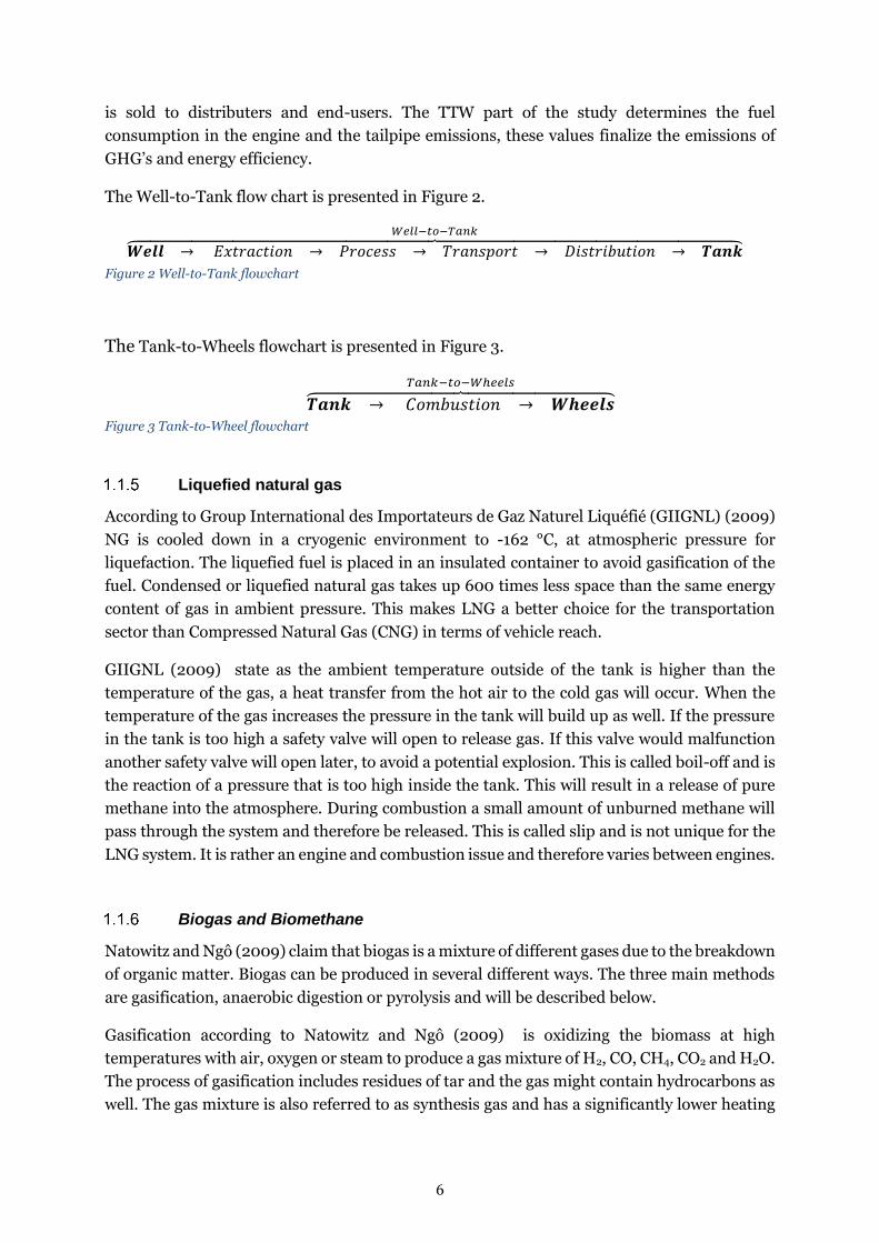
The Well-to-Tank flow chart is presented in Figure 2.

𝑾𝒆𝒍𝒍 → 𝐸𝑥𝑡𝑟𝑎𝑐𝑡𝑖𝑜𝑛 → 𝑃𝑟𝑜𝑐𝑒𝑠𝑠 → 𝑇𝑟𝑎𝑛𝑠𝑝𝑜𝑟𝑡 → 𝐷𝑖𝑠𝑡𝑟𝑖𝑏𝑢𝑡𝑖𝑜𝑛 → 𝑻𝒂𝒏𝒌⏞ 𝑊𝑒𝑙𝑙−𝑡𝑜−𝑇𝑎𝑛𝑘

Figure 2 Well-to-Tank flowchart

The Tank-to-Wheels flowchart is presented in Figure 3.

𝑻𝒂𝒏𝒌 → 𝐶𝑜𝑚𝑏𝑢𝑠𝑡𝑖𝑜𝑛 → 𝑾𝒉𝒆𝒆𝒍𝒔⏞ 𝑇𝑎𝑛𝑘−𝑡𝑜−𝑊ℎ𝑒𝑒𝑙𝑠

Figure 3 Tank-to-Wheel flowchart

Liquefied natural gas

According to Group International des Importateurs de Gaz Naturel Liquéfié (GIIGNL) (2009)

NG is cooled down in a cryogenic environment to -162 °C, at atmospheric pressure for

liquefaction. The liquefied fuel is placed in an insulated container to avoid gasification of the

fuel. Condensed or liquefied natural gas takes up 600 times less space than the same energy

content of gas in ambient pressure. This makes LNG a better choice for the transportation

sector than Compressed Natural Gas (CNG) in terms of vehicle reach.

GIIGNL (2009) state as the ambient temperature outside of the tank is higher than the

temperature of the gas, a heat transfer from the hot air to the cold gas will occur. When the

temperature of the gas increases the pressure in the tank will build up as well. If the pressure

in the tank is too high a safety valve will open to release gas. If this valve would malfunction

another safety valve will open later, to avoid a potential explosion. This is called boil-off and is

the reaction of a pressure that is too high inside the tank. This will result in a release of pure

methane into the atmosphere. During combustion a small amount of unburned methane will

pass through the system and therefore be released. This is called slip and is not unique for the

LNG system. It is rather an engine and combustion issue and therefore varies between engines.

Biogas and Biomethane

Natowitz and Ngô (2009) claim that biogas is a mixture of different gases due to the breakdown

of organic matter. Biogas can be produced in several different ways. The three main methods

are gasification, anaerobic digestion or pyrolysis and will be described below.

Gasification according to Natowitz and Ngô (2009) is oxidizing the biomass at high

temperatures with air, oxygen or steam to produce a gas mixture of H2, CO, CH4, CO2 and H2O.

The process of gasification includes residues of tar and the gas might contain hydrocarbons as

well. The gas mixture is also referred to as synthesis gas and has a significantly lower heating

7

value (LHV) compared to natural gas. Though the gas can be burned directly or going through

a purification process and later be used as a fuel.

Moreover, Natowitz and Ngô (2009) describe that anaerobic digestion is commonly used both

for biogas production facilities and in the nature. It is a biological process which involves

bacteria that decompose organic material in an area without oxygen. For biogas facilities the

oxygen free container used is called a digester which can be used for many types of feedstock.

The composition of biogas produced under these conditions is predominantly 60-70%

methane and 30-40% carbon dioxide. Biogas has the potential of being purified to receive a

higher methane content for vehicle fuel applications. Normally 20 to 40% of the original

feedstock heating value is kept in the gas. The available methane yield from the substrates is

depending on the type of substrate together with the thermal energy used (mesophilic

temperatures of 37 °C or thermophilic temperature of 55°C).

According to Natowitz and Ngô (2009) pyrolysis is the decomposition of biomass in an oxygen

absent environment using high temperatures. The biomass is decomposed into solid-char, bio-

oil and a mixture of combustible gases. Depending on the temperature used, the proportion of

the residuals are different with the main part being bio-oil for the high temperature intervals

and short residence time. The bio-oil can then be used in diesel engine.

Another way that makes it possible to produce methane is by the CO2 methanation, an

exothermic reaction in which H2 and CO2 reacts to form CH4 and H2O (Stangeland, Kalai, Li,

& Yu, 2017). This can be used both for upgrading biogas and utilize renewable energy sources

for power-to-gas applications. This technology is still in development but should not be

ignored.

Previous research

JEC is a collaboration between the European Commission's Joint Research Centre (JEC), eucar

and Concawe (European Comission, 2019). EUCAR is an European council for automotive

R&D of several major vehicle manufacturers including BMW, Iveco and Volvo (eucar, 2019)

while Concawe is a smaller group of leading oil companies researching environmental issues

related to the industry (Concawe, 2018).

JEC mainly work with evaluations of energy use and sustainability within the vehicle and oil

industry and published a Well-to-Wheels study concerning energy use and GHG emissions of

road fuels in 2014 (European Comission, 2019).

TNO (2019) is an organisation for applied scientific research in the Netherlands that was

founded in 1932. The organisation is not part of any government or company and focuses on

research within nine areas given below.

• Buildings, Infrastructure & Maritime

• The Circular Economy and the Environment

• Defence, Safety and Security

• Energy

• Healthy living

8

• Industry

• Information & Communication Technology

• Strategic Analysis & Policy

• Traffic and Transport

The organisation TNO (2017) wrote a report called Emissions testing of two Euro VI LNG

heavy-duty vehicles in the Netherlands: tank-to-wheel emissions for the Dutch Ministry of

Infrastructure and Water Management concerning the emissions from heavy-duty truck.

The two LNG vehicles tested in the programme are the following (TNO, 2017).

• Iveco Stralis Hi-road Euro VI 400hp with an automated gear box

• Scania G340 Euro VI 340hp with a manual gear box.

According to TNO (2017) the two tested LNG vehicles were tested for on-road emissions in

urban, rural and motorway scenarios and compared with the average emissions of five tested

diesel vehicles done in 2014.

NGVA (2018) stands for the Natural & bio Gas Vehicle Association which is a European

organisation that promotes natural gas as a renewable fuel in ships and vehicles. The

association was founded in 2008 and consists of 127 members from 31 countries. The

organisations members include companies and national associations from both the gas

suppliers’ and distributers’ side as well as the manufacturing side.

thinkstep wrote a report (2017) about the Well-to-Wheels emissions of natural gas and diesel

called “Greenhouse Gas Intensity of Natural Gas” for the Natural & Bio Gas Vehicle Association

(NGVA) Europe in 2017. This was done in collaboration with 27 partners in the transport

industry, including Scania. Founded in 2008, NGVA Europe is the European stakeholder that

promotes the use of natural gas and renewable methane as a fuel mainly in vehicles and ships.

The report (2017) consists of data for the Well-to-Wheels emissions and energy demand

related to the life cycle of gas and diesel using data received from 2014 and 2015. Their method

was to send out questionnaires to the respective producers of the different fossil fuels. The data

related with the upstream emissions and energy demand was performed for eight countries

while the Well-to-Tank information was gathered from a set of 37 companies including Shell

and Statoil.

In some cases by thinkstep (2017), the values received were measured, and, in some cases, only

estimated which results in some level of uncertainty. For the values related to the LCA of

transportation the LCA software GaBi is used and compared with other sources. The data

retrieved is for the fuel consumption of different vehicles and the methane emissions. For the

fuel consumption, values are based on round-trip.

Transport and environment (T&E) (2019) are an association founded in 1990 and currently

represents 58 organisations from 26 countries in Europe. Their focus is to contribute with

research to inform decision makers to change global policies within the sustainable transport

sector and achieve the greatest possible environmental benefits.

9

T&E wrote a report called “CNG and LNG for vehicles and ships - the facts” in (2018) which

are referring to the data collected by JEC in 2014. Except the values from JEC, T&E are

comparing data collected by Exergia in 2015. T&E assumes higher upstream methane emission

from LNG which results in a potential increase of both energy demand and GHG emissions.

The main work T&E do in the report is comparing different supply chains from different

studies.

Problem statement

LNG has a higher density than CNG, which makes LNG a potential substitute in the

transportation sector. Including aspects such as the condensation process and the potential

boil-off together with other energy costly factors, the total energy demand is uncertain. The

study of the liquefaction process and the potential boil-off must be done to see if the overall

emissions are lower compared to diesel. LNG can be transported both in liquid form and by

pipelines before going through the liquefaction process which might affect the potential exergy

depending on the total distribution distance. Direct comparisons between fuels in different

units, such as kg and litres, cannot be done in a fair way. Therefore, specific properties data

must be gathered for diesel and LNG.

Liquefied biogas (LBG) has similar properties as LNG and could be used for the same purpose.

Biogas can be produced with different methods from different substrates which could change

the environmental benefit of using LBG. Therefore, it is also vital to gather data for LBG

production and involve it in the study.

Aim

The aim of this degree project is find under what circumstance the use of LNG and LBG is more

beneficial to use as a fuel in the heavy-duty truck industry when compared to diesel. This will

concern energy demand, greenhouse gases, and particulates.

Research questions

• What are the main factors contributing to energy input and emissions in the production

path (WTT) for the specified fuels?

• How do different substrates used in the anaerobic digestion affect energy demand and

potential GHG emissions in LBG production?

• What is the relationship between fuel consumption, energy input and emissions?

• How much methane is released from the gas vehicle during boil-off and maintenance

and how does this affect the overall WTW emissions?

• What is a fair way to compare LNG, LBG, and diesel?

10

Delimitation

This degree project will not focus on the economic aspects of the operation process nor

potential subsidies for any of the fuels within the research work. This includes costs and

eventual emissions and energy demand from locating wells and creating the buildings. Ethical

aspects such as using land to grow crops for fuel production instead of food will not be

considered or investigated. Chemicals used for extracting and producing crude oil will not be

taken into consideration either. The water footprint for the fuel production will not be

considered.

Contribution to field of study

The findings of this degree work will clarify under what circumstance the use of LNG and LBG

is more beneficial to use as a fuel in the heavy-duty industry when compared to diesel. Having

the Well-to-Wheels analysis with several different cases of both LBG, LNG and diesel together

will simplify for the consumer in terms of choosing the most environmentally friendly fuel. The

impact of boil-off and maintenance have also been included.

11

2 METHOD

This degree project is a case study focused on the “Well-To-Wheels” comparison between the

fuels LNG, LBG and Diesel. This was done by first doing a comprehensive literature study

including the energy required and the GHG emissions for the Well-to-Tank and the Tank-to-

Wheels. The WTT includes production and transportation of the primary fuel as well as the

production and distribution of the road fuel. The TTW is the combustion of the road fuel in the

truck.

The report made by JEC was used as a reference when comparing the data with other scientific

reports due to their extensive work in the Well-to-Wheels study in 2014. The JEC report

contained many scenarios and assumptions for NG and biomass which were further analysed.

As natural gas can either be transported in pipelines or as LNG directly in tanks, additional

research of these two methods were made to find the inflection point on which the energy

demand is higher for one of the alternatives. This was done by finding the amount of energy

required for long distance and the volume transported and comparing those values with the

ones for the shorter transport distance using linear interpolation.

Along with the different types of transportation methods, the distance required depends on the

source as well as the end user. Several cases were made to compare different transportation

methods as well as the transportation distance. This includes the possibility to transport NG

and diesel by ship and by pipeline together with different distribution distances and methods.

The upgrading of raw natural gas to pipeline quality can be done using several different

methods. These methods have been compared both with energy demand and user frequency

in mind. The methods used for upgrading raw natural gas is the same used for the upgrading

of biogas with the difference in size and energy demand.

A literature study was made for the methane yield and energy demand for the production of

biogas. This includes finding active biogas plants and compare the data with more generalized

literature. The focus was on anaerobic digestion of household waste, manure and maize due to

the wide use of these substrates in Europe. Considering the differences in energy demand and

production quantity, the average values have been used to calculate the overall energy demand.

Assuming that the biogas plant is positioned close to the retail station regardless of the

substrate used, the scenarios after the production of biogas is the same.

The gathering of information included interviews with engine development engineers

positioned at Scania in Södertälje. The interviews were both structured and non-structured

open case questions. This was done to fully understand the difficulties of measuring emissions

and fuel consumption. The meetings and interviews resulted in findings of previous studies

concerning the fuel consumption, emissions and possible maintenance.

Calculations have been studied on the pressure build up in the tank depending on time and

temperature to analyse the boil-off. This was done using MATLAB and common

thermodynamic and heat transfer equations. Previous empirical data had been used to verify

12

the calculations which were used to add cases to the LNG TTW work. The methane emissions

have been evaluated using the most recent GWP values to increase the validity of the work.

Several cases were made to analyse the fuel consumption of diesel, LNG and LBG trucks. This

included the consumption of AdBlue in the diesel vehicle and the emissions and energy

required in the AdBlue production. Additional sensitivity analyses were made in the WTT

section by changing the comparison factors with ±10% to compare the results with the

possibility of having fuel from a bad production site.

The results have been compared with other previous studies both for LNG and LBG to validate

the result. For additional verification, internal classified studies and values have been used but

have not been published in this work. Instead public data have been collected to achieve fuel

consumptions and emissions for similar vehicles in size, weight and power.

The study was divided into cases to clearly state the different parameters surrounding the

evaluations and conclusions of the result. The cases produced was compared with the diesel

reference value from JEC (2014).

Well-to-tank Cases

The cases in this section covers the energy demand and GHG emissions for the three different

fuels in the WTT-part of the study.

For LNG, seven cases were constructed to have a large enough set of outcomes. These cases

were made with a change in transportation distance and method as well as for both on and off-

site liquefaction. The extraction and processing assumed to be the same with the change in

transportation distance and the sequence of the steps. The cases explained can be visualized in

Figure 4. All fuel chains will end in the combustion of the truck were a variation of fuel

consumption will be used.

Figure 4 LNG case visualization

13

LBG has a slightly different production chain compared to LNG and is therefore visualized in

Figure 5 were the only difference is the substrates used and the cultivation energy for maize.

Figure 5 LBG case visualization

Diesel is presented as two different cases in Figure 6, the cases differ in terms of distribution

only. One case used distribution by truck while the second case had distribution by pipeline.

Figure 6 Diesel case visualization

14

3 LITERATURE STUDY

In the literature study the three fuels will be described first, followed by the steps of a WTW

analysis of the fuels for heavy-duty trucks. Starting with fuel production, processing and

purification, fuel transportation and local fuel distribution. Followed by fuel consumption and

vehicle emissions.

Natural gas characteristics

JEC (2014) state that natural gas (NG) is generally associated with stationary applications i.e.

electricity production, industrial usage and domestic heating and is growing as a fuel in the

heavy-duty truck industry to battle CO2 emissions. The limitations of sulphur emissions have

also worked as incentive for the exploration of NG as a vehicle fuel.

According to the European Association of Internal Combustion Engine Manufacturers

(EUROMOT) (2017) the chemical composition of a gas is largely used to define the quality of a

gas. By knowing the quality, gas users and e.g. engine manufacturers can fine-tune their

engines to ensure a more efficient, stable and safer product. Noteworthy is that indicators of

the gas quality such as the Wobbe Index, calorific value and methane number must be properly

determined to guarantee the operating conditions.

According to the Council of European Energy Regulations (CEER) (2016) the Wobbe Index

(WI) is a factor for interchangeability between gases of different compositions. If two gases

have the same WI, the combustion energy output, given the conditions are identical (pressure

and valve settings) should be identical as well. The WI is a crucial parameter in minimizing

fluctuations in the gas quality of the gas grid and other operations. The WI is determined by

dividing the gross calorific value (higher heating value) with the square root of the relative

density, given below.

𝑊𝑜𝑏𝑏𝑒 𝐼𝑛𝑑𝑒𝑥 =𝐺𝑟𝑜𝑠𝑠 𝐶𝑎𝑙𝑜𝑟𝑖𝑓𝑖𝑐 𝑉𝑎𝑙𝑢𝑒

√𝑅𝑒𝑙𝑎𝑡𝑖𝑣𝑒 𝐷𝑒𝑛𝑠𝑖𝑡𝑦

The Swedish Standards Institute (SIS) (2003, 2009), state that a gas family are combustible

gases with similar burning behaviours connected by their WI range. A gas group is a sub-

category to the gas family, where the WI range is narrower, and the utilization area is specified

for a safe operation of the appliances. The gross WI for Group H in the second family, of which

natural gas is a part, have a minimum WI value of 45.7 MJ/m3 and the maximum value of 54.7

MJ/m3 (CH4 content from 87-92.5%). Group L has both lower WI values and methane content

compared to group H, with a WI from 39.1 – 44.8 MJ/m3 and methane content from 80-86%.

GIIGNL (2015) specify that the methane number (MN) is obtained from tests by a knock

testing unit and is not a thermodynamic property of gas. Therefore, it can’t be calculated from

its composition. Pure methane has a knock resistance, or, a methane number of 100, pure

hydrogen has a knock resistance, MN, of 0. Meaning that methane is a more stable gas than

hydrogen.

15

Moreover, EUROMOT (2017) states most engines has an optimal fuel efficiency if the MN is

above 80, engines can operate at lower MN’s but at the cost of efficiency and versatility for

power output variations. In Figure 7, the relation between the methane number and Wobbe

Index is shown. What is seen is that with an increase of the WI, the MN decreases, meaning

that the knock resistance decreases as well. The gases that have the same WI, but different MN

have the same energy output when combusted, but the knock resistance differs, therefore, the

composition of the gas is not identical.

Figure 7 Methane number and Wobbe Index correlation courtesy of EUROMOT.

SIS (2018) claim that in Europe, the gas grid has very limited requirements regarding the

quality of the gas, with the two main conditions being a methane number and relative density

over 65 and 0.555-0.700 respectively, therefore, countries can set their own requirements for

the gas to the utilized.

According to GL Noble Denton and Pöyry Management Consulting (2012) there are five main

benefits from a harmonisation of the methane number in the gas grid: more efficient sourcing

and transportation of the gas, greater competition between the gas suppliers, appliances can

work more efficiently with a more specific methane number and lastly, the security of the gas

supply could enhance as local producers could have a greater impact. Furthermore, with an

increase in the efficiency of the grid, the costs for customers can decrease as well as the

damages on infrastructure and environment. With a harmonised grid, expanding and

connecting to the grid will be easier.

According to Wester (2013) methane has a calorific heating value (Hs, HHV) of 890.3 MJ/kmol

or 39.813 MJ/m3 and 802.32 MJ/kmol or 35.882 MJ/m3 effective heating value (Hi, LHV) with

a density of 0.7175 kg/m3 at atmospheric pressure.

The LHV for LNG is set to 45.1 MJ/kg which is the value for the EU-mix presented by JEC

(2014). The temperature the LNG is kept at in Scania trucks is -132°C and 10 bar (Scania CV

AB, 2018b). The density of LNG varies depending on origin from 410-500 kg/m3, and 430-480

kg/m3 ( (Engineering ToolBox, 2008); (Kleinrahm, Lentner, Richter, & Span, 2017); (Unitrove,

2019)). Therefore, the density for the calculations in this study is assumed to be 450 kg/m3.

16

Diesel characteristics

According to Chevron Corporation (2007) diesel engines are used globally in transportation,

manufacturing, power generation, construction and agriculture. The engines vary depending

on the use, from small high-speed indirect-injection engines to low-speed direct-injection

engines. A diesel fuel is technically a generic term for a fuel that operates in a compression

ignition engine but is mostly known as a fuel for diesel-powered vehicles. With a continuous

development of the engines, there have also been a significant reduction of the NOx and PM

emissions from the heavy-duty trucks. With more knowledge of the effects of diesel fuels,

important modifications to the compositions of the fuels are being made to further decrease

the emissions. Where some of the most important parameters are sulphur, cetane number and

density.

Chevron Corporation (2007) assert while sulphur isn’t the sole source of PM emissions,

reducing the sulphur content linearly decreases the PM up to the point where there is no more

sulphur, with some variations from engine to engine.

Moreover, Chevron Corporation (2007) claims that similarly to the methane number in natural

gas, diesel fuels have a cetane number. By increasing the cetane number of the fuel, reductions

of NOx and PM emissions can be achieved, with NOx seemingly being reduced in all cases,

where PM is dependent on the engine. On the contrary to the linear connection between

sulphur content and PM, cetane number has a non-linear connection to the reductions, as, the

lower the starting value is, the greater the effect of increasing the cetane number.

To produce diesel from crude oil, Chevron Corporation (2007) state that a technique called

fractional distillation is used, where diesel can be separated from the crude oil at ambient

pressure in a temperature range between 200-350°C. Diesel fuel is a combination of individual

compounds, with carbon numbers ranging from 10-22. These compounds have different

chemical and physical properties, where different proportions of these will impact the

characteristics of one diesel fuel to another.

The general freezing point according to Chevron Corporation (2007) is increased with the

molecular weight. And compounds of the same class, have an increased boiling point with a

higher carbon number, likewise for the density. Therefore, lighter fuels such as gasoline that

have a lower density than diesel, will have a higher heating value on weight basis. But a lower

heating value on volume basis, presented in Table 1.

Table 1 Difference in heating values on weight and volume basis.

Net heating value

Fuel Weight basis [kJ/kg]

Volume basis [kJ/L]

Gasoline 43,33 31,83

Diesel 42,64 36,24

Note. Data from Diesel Fuels Technical Review, by Chevron Corporation (2007).

According to JEC (2014), the LHV of diesel is 43.1 MJ/kg and the density is 832 kg/m3.

17

To reduce the amount of NOx from the diesel engine, a mixture can be added for a Selective

catalytic reduction (SCR). This is normally done by adding Aqueous ammonia, NH3·H2O. Also

called AdBlue. Presented below are a set of different reactions with AdBlue that can occur

according to (Addy Majewski, 2018).

6NO + 4NH3 → 5N2 + 6H2O

4NO + 4NH3 + O2 → 4N2 + 6H2O

6NO2 + 8NH3 → 7N2 + 12H2O

2NO2 + 4NH3 + O2 → 3N2 + 6H2O

NO + NO2 + 2NH3 → 2N2 + 3H2O

In a study from Boyes, Brentrup and Ledgard (2011) the energy and GHG emissions from

producing urea are determined to 27.99 MJ/kg urea and 0.936 kg CO2eq/kg urea. The amount

of Urea in AdBlue is normally 32.5% with a density of 1090 kg/m3 (Preem AB, 2016).

Biomass characteristics

According to JEC (2014) biomass is a renewable energy source as it is organic material from

either plants or animals (eia, 2018). When biomass is burned, it does not count as emissions

as the crops itself capture CO2 emissions during the cultivation. Therefore, the emissions from

growing and processing the crops to fuel is considered and not combustion. The effect of

changing crops and/or deforestation has on emissions is not taken into consideration as

farming the lands more intensively also increases the cultivation emissions. The GHG

emissions from these processes should be considered as biofuel production emissions from

indirect land use change (ILUC). Even if ILUC reduce the carbon emissions, it is hard to

consider it, as it is not known what would have happened if the lands were left on their own

e.g. vegetation changes.

JEC (2014) present some guidelines for determining the ILUC GHG emissions, where they

categorize land and biomass after climate zone, ecological zone and type of soil to give them

carbon stock data. The fact that Land Use Changes (LUC) emissions happen over time after the

changes have been made, means the equilibrium of emissions take different time for soil and

cultivation. Therefore, a time frame of either 20 or 30 years is used for calculations.

For biofuel production JEC (2014) express that considerations to the type of soil and its

quality/erosion must be taken as different crops cannot grow everywhere. Rapeseed is grown

in the Northern half of Europe where the soil has higher organic content. Sunflower is grown

in the drier Southern Europe and has lower N2O emissions than rapeseed. Sugar beet cannot

grow on too drained soils, and, has lower N2O emissions than other grains/seeds. If the

utilization of fertilizers is too high, there is a risk of eutrophication and acidification of the soil.

The cultivation of bio-crops leads to less biodiversity, as the bio-crops are specially designed

18

to utilize the soil, the use of pesticides also decreases biodiversity. The introduction of

genetically modified organism (GMO) and non-native species can also lead to less biodiversity

as there are no natural predators in the new environment, there is also a concern from the

public to the use of GMO’s today. When it comes to the water usage, all crops need irrigation,

therefore, consideration must be taken for utilization and cultivation in e.g. water scarce

regions.

In addition, JEC (2014) declare that if the type of biomass in a location is converted to another,

e.g. rainforest into sugarcane, there will be a change in the amount of GHG emissions. There

is most likely a considerable release of carbon, both from the soil and vegetation in a conversion

of that sort. In the example with converting rainforest into sugarcane, there would be an

increase of 289 g CO2eq/MJ. However, it’s not always the case, if the conversion is from

grassland to farmed wood, a decrease, of -142.5 g CO2eq/MJ could occur.

Maize is the number one material in terms of fresh matter used in Germany for biogas

production according to EurObserv'ER (2014). The Swedish Energy agency (2017) reported

that in 2016 the most common biogas production in Sweden is co-digestion using manure and

organic household waste.

Fuel production

The fuel production chapter is divided into three major areas, the first part covers the

production of NG and crude oil, the second part biomass cultivation and lastly biogas

production.

Production of Natural gas and Crude oil

According to natgas (2013) there are three types of wells commonly used, crude oil wells, gas

wells, and condensate wells. This results in two categories of gas types. There is associated-

dissolved from oil wells and non-associated gas from the gas wells. The gas from gas wells is

normally raw NG, while the gas from condensate wells often includes other low molecular

weight hydrocarbons together with the NG. The gas extracted from underground sandstone

and limestone formations is regarded as conventional while unconventional gas refers to shale

gas or coal bed methane.

Natgas (2013) mention that if the gas is relatively free of hydrogen sulphide the gas is called

sweet gas and otherwise sour gas, though if the gas mixture contains large quantities of

hydrogen sulphide and carbon dioxide the gas is called sour gas. Raw NG contains many other

components besides methane such as H2O, CO2, H2S, CH4, and helium.

JEC (2014) distinguish that the extraction of gas, also called the production can be different

dependent on the characteristics and the location of the well. Two main locations are

categorized when discussing the energy demand for the extraction, onshore and offshore

production. The value used for extraction for NG is determined to 0.0259 MJ/MJfuel and for

diesel 0.0715 MJ/MJfuel with no consideration to origin in this study.

19

According to thinkstep AG (2017) the heating value and amount of gas losses in the gas

production in Norway 2015 is 1 013 261 kJ/tonne NG together with 92 544 kJ/tonne diesel and

136 084 kJ/tonne electricity. This was specified as data from a questionnaire to Statoil.

In the production of oil and gas JEC (2014) state that the main sources of GHG emissions come

from the extraction and pre-treatment of the oil as well as from flaring and venting (F&V) and

fugitive losses. However, at the time of the study, reporting of GHG emissions from the oil

companies were underwhelming and data was hard to come by. The oil production companies

have developed their methods for reporting and estimating GHG emissions.

Moreover JEC (2014) specify that the data for emissions and specific energy used in their study

is obtained from IOGP. IOGP represents 32% of the oil and gas production industry, but as

high as 48% of the consumed oil share in the EU. IOGP presents that 51% of their GHG

emissions are due to energy use, 35% from flaring and 14% due to venting and fugitive losses.

As IOGP at the time was the sole supplier of extensive global data from the oil and gas industry,

JEC has converted their numbers to three sources of emissions.

• 1.5 g CO2eq/MJ crude for energy use in production

• 1.0 g CO2eq/MJ crude for flaring

• 0.4 g CO2eq/MJ crude for venting and fugitive losses

Furthermore JEC (2014) however, only adopted the estimates for energy use in production,

venting and fugitives to the study. The values for flaring are obtained from the US National

Oceanic and Atmospheric Administration’s (NOAA) global satellite data. The flared gas is

however from both oil and gas production, therefore the JEC uses two scenarios to gain a range

of plausible GHG emissions from flaring. By assuming that all flared gas is from oil production

alone, the upper bound of the range is determined to 2.9 g CO2eq/MJ. The lower bound is

obtained by distributing the flaring evenly for oil and gas production, giving a value of 1.8 g

CO2eq/MJ. In the study, 2.4 g CO2eq/MJ is used as it is a midrange value rounded up. This is an

increase from the value IGOP presented of 1.o g CO2eq/MJ. The production values for crude is

given in Table 2.

Table 2 Emissions and energy demand values for oil and natural gas production.

Production values for oil and natural gas

GHG emissions [g CO2eq/MJ crude]

Energy [MJ/MJ crude]

Production energy 1.5 0.027

Flaring 2.4 0.037

Venting and fugitive losses

0.4 0.001

Total 4.3 0.065

Note. Data from Well-to-Wheels Analysis, by JEC (2014).

For NG JEC (2014) use a value of 1% v/v CO2 for venting during the production phase. For the

production a median value of 2% of the gas is used as energy. GHG emissions from the energy

use is set to 1% volume venting for CO2 and 0.4% volume of methane.

20

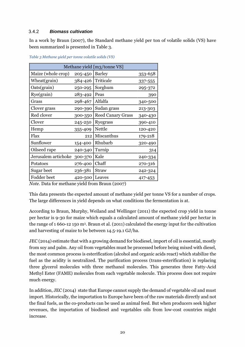
Biomass cultivation

In a work by Braun (2007), the Standard methane yield per ton of volatile solids (VS) have

been summarized is presented in Table 3.

Table 3 Methane yield per tonne volatile solids (VS)

Methane yield [m3/tonne VS]

Maize (whole crop) 205-450 Barley 353-658

Wheat(grain) 384-426 Triticale 337-555

Oats(grain) 250-295 Sorghum 295-372

Rye(grain) 283-492 Peas 390

Grass 298-467 Alfalfa 340-500

Clover grass 290-390 Sudan grass 213-303

Red clover 300-350 Reed Canary Grass 340-430

Clover 245-250 Ryegrass 390-410

Hemp 355-409 Nettle 120-420

Flax 212 Miscanthus 179-218

Sunflower 154-400 Rhubarb 320-490

Oilseed rape 240-340 Turnip 314

Jerusalem artichoke 300-370 Kale 240-334

Potatoes 276-400 Chaff 270-316

Sugar beet 236-381 Straw 242-324

Fodder beet 420-500 Leaves 417-453

Note. Data for methane yield from Braun (2007)

This data presents the expected amount of methane yield per tonne VS for a number of crops.

The large differences in yield depends on what conditions the fermentation is at.

According to Braun, Murphy, Weiland and Wellinger (2011) the expected crop yield in tonne

per hectar is 9-30 for maize which equals a calculated amount of methane yield per hectar in

the range of 1 660-12 150 m3. Braun et al. (2011) calculated the energy input for the cultivation

and harvesting of maize to be between 14.5-19.1 GJ/ha.

JEC (2014) estimate that with a growing demand for biodiesel, import of oil is essential, mostly

from soy and palm. Any oil from vegetables must be processed before being mixed with diesel,

the most common process is esterification (alcohol and organic acids react) which stabilize the

fuel as the acidity is neutralized. The purification process (trans-esterification) is replacing

three glycerol molecules with three methanol molecules. This generates three Fatty-Acid

Methyl Ester (FAME) molecules from each vegetable molecule. This process does not require

much energy.

In addition, JEC (2014) state that Europe cannot supply the demand of vegetable oil and must

import. Historically, the importation to Europe have been of the raw materials directly and not

the final fuels, as the co-products can be used as animal feed. But when producers seek higher

revenues, the importation of biodiesel and vegetables oils from low-cost countries might

increase.

21

According to JEC (2014) palm is the largest source of vegetable oil and the life span of a palm

tree is 20-30 years. This gives low cultivation input of energy compared to rape seed, as the

cultivation period is lower for rape seed. The use of fertilizers can, to some extent, be mitigated

as the biomass might be returned as mulch for further use. The oil is often extracted in small

plants close to the fields as the fruits from the palm trees ripen rapidly. The palm oil is extracted

from the fruits after they are heated and crushed. The nuts from the trees can yield oil as well,

palm kernel oil (PKO). This oil has different properties compared to the other oil from the palm

tree, but can still be used for biodiesel production. In their study, PKO and palm oil is added

together for calculations.

In their study, JEC (2014) report that burning wood increases CO2 emissions in the

atmosphere, this is however neglected as new tree grows and use CO2 in photosynthesis, so

there are no net emissions over time. If trees are cut, sequestration may change, either increase

or decrease. If trees are cut down and replaced, it might lead to a more rapid carbon

sequestration, however, it usually takes a hundred years to equal the carbon taken from the

forest. Short term bioenergy will not contribute significantly to the mitigation of climate

targets, but, will in the long-term, compared to the combustion of fossil fuels.

Moreover JEC (2014) claim that energy crops and for some “short-rotation forests” there will

be a carbon credit, as new trees are grown before harvesting of wood. If there is more

consumption than arable growth, there is a carbon debit. If branches, stumps and other

biomass from deforestation is not utilized for energy generation and is rotting in the forest it

could count as land use change emissions.

Production of biogas

Biogas is a composition of methane and carbon dioxide. The anaerobic digestion of organic

material by methanogenic bacteria can be illustrated by the following formula.

𝐶𝐻2𝑂 →1

2𝐶𝐻4 +

1

2𝐶𝑂2

The organic matter decomposition in a methanogenic ecosystem can be studied in Figure 8

Organic matter decomposition.

Figure 8 Organic matter decomposition.

22

Wellinger (2013) states that reducing the size of solid substrates to 2% of their original size

could increase the yield by approximately 20 to 25%. Using a knife mill to reduce the particle

size of wheat straw from 12.5 to 1.6 mm will require 2.8-7.55 kWh/tonne. The amount of energy

required to stir digesting slurries using a continuous stirred-tank reactor (CSTR) will require

around 10 kWh/tonne and is much higher for solid substrates. If the increase of methane yield,

and the reduction of the electrical demand for the CSTR is uncertain though.

According to (Wellinger, A. 2013), the energy demand is typically about 20% of the energy

content for physical pre-treatment, mainly from electricity and slightly less for heat. The effects

achieved in terms of increased methane yield is highly dependent on the substrates used and

could be equal to the energy required for the pre-treatment.

A non-physical way to increase the methane yield as reported by Wellinger (2013) is to increase

the temperature in a closed system and heat the substrate to a temperature of 106 to 220 °C.

This causes the pressure to increase which, after a retention time of 5-60 minutes, is released

abruptly. This results in cellular disruption due to the contained water being evaporated and

is estimated to increase the methane yield of fresh matter maize up to 25%. The increase is

measured to 250 m3 CH4 per tonne fresh matter instead of 200 m3/tonne. A similar increase is

measured on slaughterhouse residues were the yield is increased from 450 to 500 m3 CH4

/tonne fresh matter.

From a report by Uppsala Vatten och Avfall AB (UVA) (2017) the operation of the plant

Kungsängens gård is described. The plant receives both liquid and solid waste, where the liquid

waste goes directly to a settling tank. The solid waste is accepted either with or without plastic

packaging. The organic household waste is pre-treated, as it comes in plastic packaging, this is

a process where the waste is separated from the plastics.

UVA (2017) specify that after the treatment, all the solid materials are transported to a stirring

tank, where the dry solids (DS) content is diluted to 15%. From the stirring tank, the substrate

is transported to a buffer tank for storage. Before the substrate can be digested, a hygenization

of the substrate is performed. The substrate is then transferred to a hygenization tank where

the temperature in the tank must remain above 70°C for an hour to ensure the digestion is as

predicted. After the hygenization is done, the digestion takes place in the digestion chamber,

under anaerobic conditions and a thermophilic process where the temperature is 52°C.

In 2017, the plant received 35 000 tonnes of waste, with 29 500 being organic household waste

and 5 500 tonnes industrial waste (e.g. slaughterhouse and restaurants). The production of

biogas reached 5 Mmn3, which was converted to 31 900 MWh. The produced biogas was either

used for internal heating or being upgraded to biomethane, where 7 % was used for heating

and 89% was turned into biomethane, 4% was flared and 0.3% was estimated as methane slip.

(The figures add up to 100.3%, probably due to rounding of values from the plant.) The plant

used 41 kWhel/tonne waste for electrical parts in the process and 96 kWh/tonne waste for

heating.

According to Wellinger (2013) the electricity demand for using the CSTR is estimated to 15-23

kWhel/MWhHi for liquid feedstock and 19-27 kWhel/MWhHi for more solid content, such as

energy crops. The most common fermentation temperature is mesophilic digestion, for which

23

the temperature is 39°C. The energy needed for keeping the defined temperature, changes

with the ambient temperature following the seasons. In Central Europe the heat demand for

organic residues, manure or energy crops is estimated to be 5-15% of the energy available in

the produced biogas.

JEC (2014) distinguish that the production of biofuel still requires the use of fossil energy,

which must be considered in calculations of this sort. There is not only CO2 emissions to

consider with the production of biofuels, but also N2O emissions, both from nitrogen fertilizer

production and field emissions. The high GWP of N2O (298) makes it considerable even though

the amount of emissions are very low. The sources of N2O emissions are one direct and two

indirect pathways, nitrogen added/released to the soil, volatilization of NH3 and NOx as well

as leaching and runoff of nitrogen respectively. Measuring N2O emissions from the soil is

expensive and not available in all locations or for all crops. As N2O emissions can vary

drastically over short distances and years, there is no standardized tests regarding the

emissions.

According to JEC (2014) the cultivation of maize produces 45.1 g CO2eq/MJ fuel where 27.9 g

of this is N2O. The figures are given as emissions per MJ produced fuel as different soils and

input (crops) gives different amounts of production per hectare, which is not clearly

understood. This is excluded when dividing per MJ fuel. With the use of nitrogen fertilizers,

there will be acidification of the soil, however this can be neutralized either by using

agricultural lime or carbonates.

The average Swedish bio-methane production results in greenhouse emissions of 8 g

CO2eq/MJ according to Energigas Sverige (2018). For bio-methane production with manure

as the substrate, the emissions are -20 g CO2eq/MJ given in Table 4. These values come from

using the International Organisation for Standardization (ISO)-method for the calculations. If

the Swedish sustainability calculation (HBK)-tool is used the values are instead in average 18.9

g CO2eq/MJ. Non-upgraded biogas as well as bio-methane and their corresponding emissions

in g CO2eq/MJ and the used methods can be viewed in the Table 4.

Table 4 CO2eq emissions using different methods and substrates

Fuel Emissions [g CO2eq/MJ] Method

Biogas 0.6 ISO

Biogas 12.8 hbk

Bio-methane 8 ISO

Bio-methane 18.9 hbk

Biogas from manure -20 ISO

Note. Data for biogas from Energigas Sverige (2018).

Ahlgren, Börjesson, Lundgren and Nyström (2013) state that manure slurry has direct

emissions of 11.4 g CO2eq/MJ using the RED method and -20 g CO2eq/MJ including the use

of the substrate as future fertilizer. For organic household waste the emissions are 10.3 and -

2.3 g CO2eq/MJ respectively. For maize the emissions are 30.7, 41.3 and 42.6 g CO2eq/MJ

while also mentioning that maize have emissions related to the cultivation, harvesting and

transportation between 16 and 23 kg CO2eq/GJ biomass. The values are presented in Table 5.

24

Table 5 Manure, Organic waste and Maize CO2 emissions

Substrate Direct emission [g CO2eq/MJ]

RED-method [g CO2eq/MJ]

Larger boundaries [g CO2eq/MJ]

Manure slurry 11.4 14.9 -20

Organic household waste

10.3 9.4 -2.3

Maize 41.3 42.6 30.7

Note. Data for CO2 emissions of manure, organic household waste and maize from Ahlgren,

Börjesson, Lundgren and Nyström (2013)

In a Well-to-Wheels analysis done by Andersson et al. (2016) the energy input for biogas

production is 0.12-0.13 MJ/MJ using the ISO-method and 0.16-0.17 MJ/MJ using the RED

method. The values from the ISO calculations are shown in Table 6.

Table 6 Direct energy input for biogas production (MJ/MJ biogas) using the ISO-method

Energy Input

Origin Specific step 30 GWh 100 GWh

Food Waste Transport (diesel) [MJ/MJ] 0,036 0,036

Pre-treatment (electricity) [MJ/MJ] 0,015 0,015

Transport Feedstock (diesel) [MJ/MJ] 0,011 0,015

Digestate (diesel) [MJ/MJ] 0,01 0,014

Process

energy

Electricity [MJ/MJ] 0,023 0,023

Heat [MJ/MJ] 0,08 0,08

Spreading of digestate (diesel) [MJ/MJ] 0,007 0,007

System

expansion

Avoided Spreading of manure (diesel)

[MJ/MJ] -0,003 -0,003

Avoided production of mineral fertilizers

[MJ/MJ] -0,061 -0,061

Total energy input [MJ/MJ] 0,12 0,13

Note. Data for energy input in biogas production from Andersson et al. (2016).

25

The GHG emissions calculated by Andersson et al. (2016) are determined to -9.5 g CO2eq/MJ

using the ISO-method and are presented in Table 7. This is done by using the GWP value for

methane of 34 and 298 for N2O.

Table 7 GHG emissions from biogas production using the ISO-method

Emissions [g CO2eq/MJ biogas]

Biogas production

CH4 Slip 0,06

CH4 from flare 0,02

Handling of digestate

CH4 from digestate storage 0,11

N2O from spreading of digestate 0,05

System expansion

CH4 from storage manure -0,14

N2O from storage and spreading of manure -0,06

CO2 from production of mineral fertilizer -4,36

CH4 from production of mineral fertilizer -0,01

N2O from production of mineral fertilizer -0,01

CO2 from spreading of mineral fertilizer -0,02

Changes in soil carbon -5,17

Total GHG emissions -9,5 Note. Data for GHG emissions in biogas production from Andersson et al. (2016).

According to Ahlgren and Assefa Hagos (2018) the gas yield varies with different origins of

manure. Cattle slurry is estimated to have a gas yield of 0.21 m3/kg-DS while swine slurry has

a higher yield at 0.29 m3/kg-DS. The gas yield from organic household waste from the typical

Danish household is measured to 0.43 m3/kg-DS. The heat and the electricity demand for the

digestive process together with the potential gas yield is presented in Table 8.

Table 8 Gas yield and energy demand for organic waste and manure

Substrate Gas yield [m3/kg DS]

Heat [MJ/Mjraw gas]

Electricity [Mje/Mjraw gas]

Municipal organic waste 0,43 0,0865 0,0622

Manure-Cattle slurry 0,21 0,0962 0,019

Manure-swine slurry 0,29 0,0962 0,019 Note. Data for energy demand and gas yield of waste and manure from Ahlgren and Assefa

Hagos (2018).

Höjgård and Wilhelmsson (2012) state that emissions from swine and cattle slurry varies

depending on geographical location, in the south of Sweden, the methane emissions per tonne

cattle slurry is 1255 g CH4/tonne and in central Sweden it is 376 g CH4/tonne. Therefore, in

Table 9 average values for Sweden are listed. For calculations of the CO2 equivalents, Höjgård

and Wilhelmsson (2012) use a GWP of 25 for methane.

26

Table 9 Effect of manure usage for biogas production in Sweden

Swine Cattle

Methane yield storage [g CH/ton slurry] 2213 815,5

Methane yield storage [Nm3 CH4/tonne slurry] 16 14

Biogas yield [g CH4/Nm3 CH4] 138,313 58,25

CO2eq from storage [g CO2eq/Nm3 CH4] 3457,813 1459,25

Production of biogas [g CO2 eq/Nm3 CH4] -2076,0955 -1124,669 Note. Data for how the potential CO2 equivalents saved by biogas production of manure

from Höjgård and Wilhelmsson (2012).

The difference in emissions dependent on the location of the production in Sweden can be seen

in Table 10 from Höjgård and Wilhelmsson (2012). The difference in emissions from swine in

central production and south production is over 2000 g CO2 eq/Nm3. For Cattle the difference

is 1500 instead g CO2 eq/Nm3. The higher negative value for both of the substrates is in the

southern part of Sweden.

Table 10 Net effects on emissions from biogas production (per Nm3 methane)

South Central

Swine slurry [g CO2 eq/Nm3] -3283,004 -869,187

Cattle slurry [g CO2 eq/Nm3] -1909,49 -339,848

Note. Data for how the potential CO2 equivalents saved by biogas production of manure

from Höjgård and Wilhelmsson (2012).

Processing and purification

thinkstep AG (2017) report that after extraction, the raw NG, must be processed to remove free

liquids and NG condensate before transportation. The transportation is often by pipeline, to a

gas purification plant to remove acid gases (CO2, H2S). This process is estimated to require 50

232 kJ/t. The purifying can be done using different methods. Historically the most used

method is called Amine treating. There is also a method of using polymeric membranes, both

are used to remove the acid gases. Removing the sulphur from the mixture can be done by

using the Claus process, Contact process or a WSA (wet sulphuric acid process).

According to thinkstep AG (2017) the gas is at this point referred to as tail gas, which still

contains water vapour. The water vapour needs to be removed and the gas dehydrated before

removing the possible mercury and Liquefied Petroleum Gas (LPG). The purifying and

liquefaction of the gas require a total of 3 627 135 kJ/t. Worth noticing is that in this case the

GWP100 value chosen for methane is 25, the AR4 value, which is lower than the AR5 value of

28. This was done to increase the possibility of comparing the report with other, similar

studies.

For all the steps above thinkstep AG (2017) estimated that the sum of energy required is 4 919

MJ/tonne NG. The weighted average value of GHG for gas production, processing and

liquefaction is 4.7 g CO2e /MJ (LHV) in EU.

27

JEC (2014) state that crude oil is mostly transported in its original state and is refined in local

refineries closer to the market. In Europe e.g., except for jet fuel and some gas oils, fuels based

on crude oil is produced in European refineries. The process of refining crude oil consists of

separating and removing different components in the crude such as sulphur. Lastly, conversion

from heavy to lighter molecules is performed as the market request both. To process the crude

oil, the refineries use 6-7% of the energy from the oil itself. Even though the energy and

emissions in the refining process are well-documented, they are not divided into the separate

processes or products, but for the refinery as a whole. The energy need for diesel refining is 0.1

MJ/MJfuel and the GHG emissions are 8.6 g CO2eq/MJ. The finished products are mostly

transported to a depot using pipelines, trains or barges. However, some of the fuel is

transported by trucks directly to retail stations as well.

Biogas upgrading technologies

According to Wellinger (2013) the composition of biogas is approximately 55% methane and

45% carbon dioxide. Upgrading the gas to natural gas quality involves the removal of CO2. A

common method used for upgrading the biogas is the water scrubber which demand between

0.2-0.25 kWhel/m3 raw biogas. Normal methane recovery during this process is in the range of

98-99.5%, this results in methane losses of 0.5-2%. A chemical absorption method could be

used to minimize the amount of methane losses but will have a higher energy demand in the

range of 0.46-0.97 kWh/m3 raw gas. If the gas is to be injected to the gas grids, which operates

between 0.4-8 MPa, additional electric energy of 0.2 kWhel/m3 biomethane is required. During

the compression of the gas, energy in the form of heat can be recovered and used to supply heat

for the fermentation.

Furthermore, Wellinger (2013) present another upgrading method as well, cryogenic

upgrading. This is done by cooling the gas and separating CO2 and H2S due to the difference in

condensation temperatures. The electricity demand for the cooling process is estimated to be

between 0.18-0.25 kWhel/mn3 with methane losses in the range of 0.1-1%.

UVA (2017) present that at the plant Kungsängens gård, the gas from the digestion chamber

is collected in a gas dome before being upgraded to biomethane. The biomethane has a

methane content of above 97%. The upgrading plant is connected to a combustion plant that

incinerates almost all methane slip, just 0.3% of the received methane slips through the

complete process.

Liquefaction process

Liquefaction is a process where either a gas, or a solid, is changing phase into a liquid. This can

be done either by changing the temperature or the pressure according to the laws of

thermodynamics. For a gas, this is normally done by lowering the temperature and therefore

condensate the gas, for natural gas this greatly reduces the volume of the fluid. Apart from

methane other substances will be removed during the process due to different condensation

temperatures, and therefore increasing the methane composition.

28

Ahlgren and Assefa Hagos (2018) state that the three most common types of liquefaction plants

are the propane pre-cooled mixed refrigerant, single mixed refrigerant (SMR), and the reverse

Brayton cycle or expander process. These can be used both for large and small operations were

the SMR is most common in smaller plants while the propane pre-cooled method is mostly

used for larger operations and can reach an efficiency of 90.7%.

According to Ahlgren and Assefa Hagos (2018) the electricity demand during liquefaction for

the Lidköping LBG plant is at maximum 1.56 kWh/kg LBG and with a gas leakage estimated

at 0.05% of the gas throughout the system. In this case the electricity used is assumed to be

grid consumed and for non-local LNG liquefaction plants the energy demand is estimated at

0.09MJ/MJLNG. JEC (2014), imply the energy needed for liquefaction is 0.08 MJ/MJfuel

independently if the liquefaction is performed on- or off-site.

Fuel Transportation

According to JEC (2014) crude oil is mostly transported overseas from the production sites to

the refineries in Europe by ship with the type of ship depending on the travelling distance. The

crude from the Persian Gulf is often transported in Very or Ultra Large Crude Carriers (V-

/ULCC) and they carry between 200-500 kt. Ships from the North Sea or Africa are often

smaller, at around 100 kt, as the distance is shorter. Pipelines are mostly used to transport the

crude from the production site to the loading terminal. At the terminals, the energy usage is

set to 0.0122 and 0.0129 for loading and unloading the ship respectively. The energy use for

transportation originates from the Middle East and the estimated energy self-use is 0.0121

MJ/MJfuel which corresponds to 0.8 g CO2eq/MJ for diesel transportation if the ship is fuelled

by heavy fuel oil. For an LNG carrier, the energy usage is determined to 0.07 MJ/MJfuel.

In addition, JEC (2014) state that the greatest energy requirement for NG comes from the

transportation in pipelines, with some pipelines being 4000-7000 km. These pipelines need

compression stations along the pipeline to ensure the pressure is high enough, so the gas does

not condensate. The compression stations utilize some of the NG to operate. The pipelines

today operate at 6-8 MPa, however new technologies might increase the pressure utilized in

the pipelines. With an increase in pressure with a constant diameter and flow, the energy need

can be decreased by a factor of 2-3. In their study, JEC assume 9.6% of the NG is used at the

compression stations for a 4000 km pipeline. For each 1000 km, 0.13% of the transported

methane is assumed to be lost as leakage.

Moreover, JEC (2014) claims that if the transportation distance is extensive, an alternative to

transport NG in pipelines is to ship the NG as LNG. The shipping distance in the study is

assumed to be 5000-6000 nautical miles with an energy demand of 0.07 MJ/MJfuel. The

evaporation rate of gas in a cryogenic carrier is determined by 0.15 %/day, with an average

speed of 19.5 knots and average distance of 5500 nautical miles. Long-distance pipeline

transportation is assumed to be proportionate to the distance travelled, for 2500, 4000 and

7000km the values are 0.0584, 0.1023 and 0.1809 MJ/MJfuel respectively.

29

According to Wellinger (2013) normally for local biogas plants the transportation in terms of

energy input is low or negligible and is associated with the fuel consumption of the tractor,

truck and wheel loaders. For liquid substrates there is the option to pump the mixture using

electricity. For centralized biogas plants the energy demand for the transportation could

significantly increase with a transportation distance up to hundreds of kilometres.

Local fuel distribution

JEC (2014) assert that Europe’s extensive network of pipelines for NG mainly operate at two

different pressure levels. The high-pressure pipelines operate at 4-6 MPa and supply industries

and the low-pressure pipelines, which are the local pipelines. The low-pressure pipelines

operate at 0.4 MPa, however a few countries still have 0.1 MPa in their low-pressure pipelines.

The length of the high-pressure pipelines is set to 500 km. The energy needed to distribute the

gas is 0.01 MJ/MJfuel for local distribution with high-pressure pipelines. Diesel distribution by

pipeline is set to 0.0095 MJ/MJ and the emissions to 0.6 g CO2eq/MJ.

For road transport JEC (2014) consider a diesel truck with a payload of 40 tonnes and the

distribution range is set to 500 km, with a value of 0.0216 MJ/MJfuel and GHG emissions of

3.7339 CO2eq/MJfuel.

Furthermore JEC (2014) claims that the dispensing of diesel and LNG at retailers varies as the

two fuels have different characteristics. Diesel have a value of 0.0111 MJ/MJfuel and GHG

emissions of 0.5 g CO2eq/MJ while LNG have 0.0001 MJ/MJfuel and GHG emissions of 0.01 g

CO2eq/MJ.

From the study made by thinkstep (2017) the EU Total GHG Well-to-Tank result, as well as all

other regional results, is dominated by Natural Gas production, processing and liquefaction

(77%), followed by feedstock transportation (15%), fuel dispensing (6%) and storage and

distribution (2%). With a total carbon footprint of LNG of 19.9 g CO2eq/MJ.

Fuel consumption

Data have been empirically collected from vehicles of the same engine power, weight and route

for both diesel and LNG. This resulted in values corresponding to a fuel consumption of 11%

higher for LNG vehicles with 18% lower powertrain efficiency.

The New Truck Generation (NTG) gas vehicle have an efficiency of 40% while the diesel engine

has an efficiency of 44% and a fuel consumption that is 7% lower than for gas vehicles in

average, according to Améen (2015).

The average gross trailer weight (GTW) for the Scania transport laboratory is 34 tonnes which

results in an average fuel consumption of 27.4 l/100 km diesel and 1.42 l/100 km AdBlue

(Scania Transportlaboratorium AB, 2015).

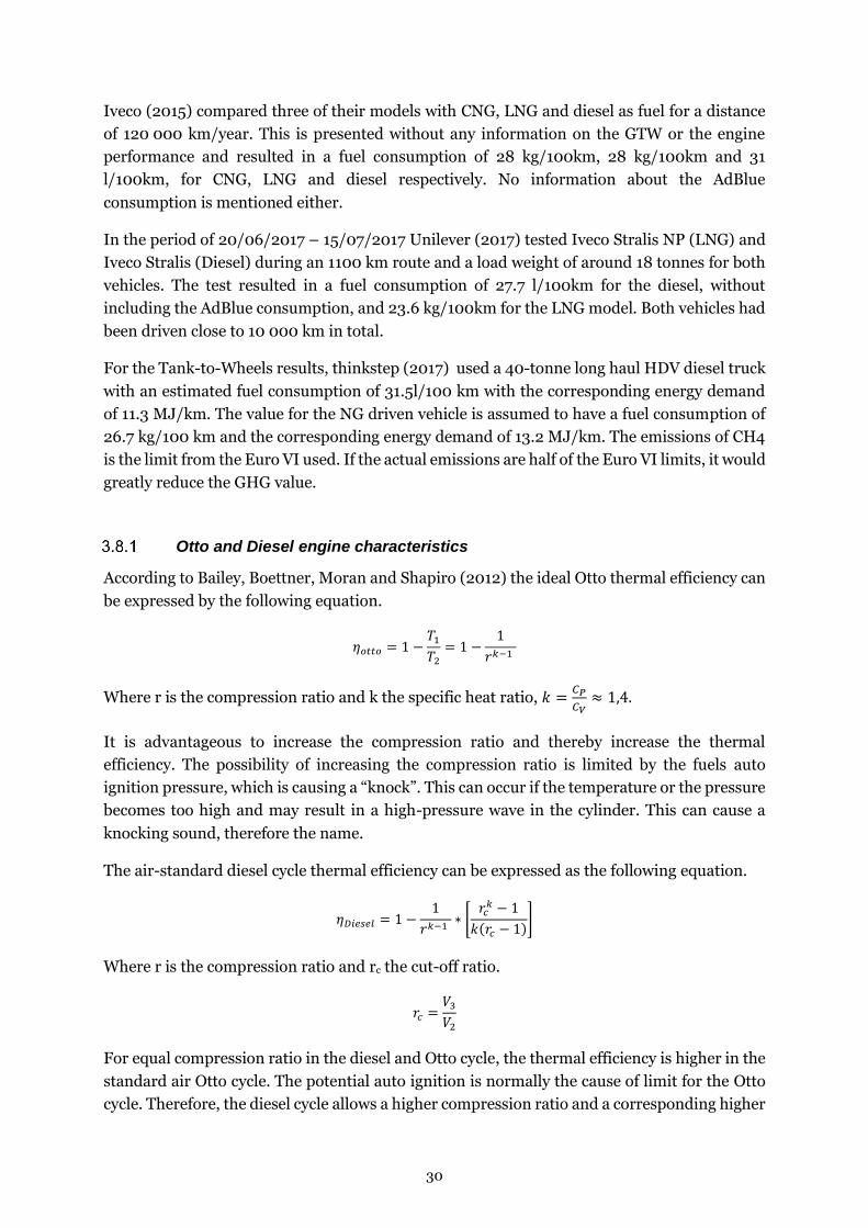
30

Iveco (2015) compared three of their models with CNG, LNG and diesel as fuel for a distance

of 120 000 km/year. This is presented without any information on the GTW or the engine

performance and resulted in a fuel consumption of 28 kg/100km, 28 kg/100km and 31

l/100km, for CNG, LNG and diesel respectively. No information about the AdBlue

consumption is mentioned either.

In the period of 20/06/2017 – 15/07/2017 Unilever (2017) tested Iveco Stralis NP (LNG) and

Iveco Stralis (Diesel) during an 1100 km route and a load weight of around 18 tonnes for both

vehicles. The test resulted in a fuel consumption of 27.7 l/100km for the diesel, without

including the AdBlue consumption, and 23.6 kg/100km for the LNG model. Both vehicles had

been driven close to 10 000 km in total.

For the Tank-to-Wheels results, thinkstep (2017) used a 40-tonne long haul HDV diesel truck

with an estimated fuel consumption of 31.5l/100 km with the corresponding energy demand

of 11.3 MJ/km. The value for the NG driven vehicle is assumed to have a fuel consumption of

26.7 kg/100 km and the corresponding energy demand of 13.2 MJ/km. The emissions of CH4

is the limit from the Euro VI used. If the actual emissions are half of the Euro VI limits, it would

greatly reduce the GHG value.

Otto and Diesel engine characteristics

According to Bailey, Boettner, Moran and Shapiro (2012) the ideal Otto thermal efficiency can

be expressed by the following equation.

𝜂𝑜𝑡𝑡𝑜 = 1 −𝑇1𝑇2= 1 −

1

𝑟𝑘−1

Where r is the compression ratio and k the specific heat ratio, 𝑘 =𝐶𝑃

𝐶𝑉≈ 1,4.

It is advantageous to increase the compression ratio and thereby increase the thermal

efficiency. The possibility of increasing the compression ratio is limited by the fuels auto

ignition pressure, which is causing a “knock”. This can occur if the temperature or the pressure

becomes too high and may result in a high-pressure wave in the cylinder. This can cause a

knocking sound, therefore the name.

The air-standard diesel cycle thermal efficiency can be expressed as the following equation.

𝜂𝐷𝑖𝑒𝑠𝑒𝑙 = 1 −1

𝑟𝑘−1 ∗ [

𝑟𝑐𝑘 − 1

𝑘(𝑟𝑐 − 1)]

Where r is the compression ratio and rc the cut-off ratio.

𝑟𝑐 =𝑉3𝑉2

For equal compression ratio in the diesel and Otto cycle, the thermal efficiency is higher in the

standard air Otto cycle. The potential auto ignition is normally the cause of limit for the Otto

cycle. Therefore, the diesel cycle allows a higher compression ratio and a corresponding higher

31

thermal efficiency. An internal study made on Scania revealed that the powertrain efficiency is

18% lower for the LNG Otto vehicle than for the diesel vehicle.

Vehicle emissions

According to the Intergovernmental Panel on Climate Change (IPCC) fifth Assessment report

(AR5) (2014) the estimated lifetime for methane in the atmosphere is 12.4 years. For N2O the

estimated lifetime is 121 years. The GWP value for these emissions vary with the timeframe for

the calculations of the GWP. The standard timeframes are 20 and 100 years and the values for

each emission and year is given in Table 11.

Table 11 Global Warming Potential Values for CH4 and N2O

IPCC's AR5 Global Warming Potential

Emission GWP100 GWP20

CH4 28 84

N2O 298 264 Note. Data for GWP values of CH4 and N2O with different timeframes from IPCC (2014).

JEC (2014) use an older GWP for methane of 25.

GHG emissions from tail-pipe

From the report by TNO (2017) there is some methane slip that could be measured before the

three-way catalyst was warmed up. This resulted in a 10 grams emission for ambient

temperatures of 0-5 °C during cold starts. TNO is using the 2013 IPCC AR5 to determine the

GWP100 of methane to 34 as they include positive feedback, which results in a CO2eq value

corresponding to 340 grams. With the methane slip for both the vehicles tested the emissions

are of the order 2 CO2eq/km. The overall results concluded that the LNG vehicles had 5-10%

lower CO2 emissions compared to the Diesel engines.

The ICCT (2013) states that the Euro VI standard is a vehicle emissions standard to limit the

air pollution from the vehicle industry. It was first introduced in 1992 as Euro 1, and the latest,

Euro VI was introduced in 2013 and in 2014 all newly manufactured vehicles must follow the

regulations. The regulations for Euro VI heavy-duty trucks are presented in Table 12.

32

Table 12 Euro VI Heavy-duty regulations.

EURO VI Heavy-Duty Vehicle regulations

Emission Limits

CO [g/km] 4

HC [g/km] 0,16

CH4 [g/km] 0,5

NOx [g/km] 0,46

PM [g/km] 0,01

PN (#/km) 6E+11

Ammonia (ppm) 0,01

Fuel Sulfur Limit (ppm) 10 Note. Data for Euro VI regulations from ICCT (2013) and European Commission (2014).

According to DieselNet (2017) the limit to N2O emissions are 0.133 g/kWh (0.10 g/bhp-hr).

From Transportstyrelsen ( (2018a); (2018b)) the emissions according to the World

Harmonized Transient Cycle (WHTC) of the two reference vehicles are obtained. These values

are presented in Table 13.

Table 13 Emissions from the reference vehicles.

Emission Diesel LNG

CO [mg/kWh] 28,2 343,3

THC [mg/kWh] 9,1 -

NOx [mg/kWh] 387,1 173,3

Particulates [mg/kWh] 2,6 2,5 Note. Data for two reference vehicles from Transportstyrelsen ( (2018a); (2018b)).

The emission factors for the fuels presented in Table 14 represents 100% oxidation of fuel

carbon content.

Table 14 CO2 emission factors for LNG and Diesel

Road transport default CO2 emission factors and uncertainty ranges

Diesel oil [kg/TJ] 74 100 72 600 74 800

Liquefied Natural Gas [kg/TJ] 56 100 54 300 58 300 Note. Data for CO2 emission factors from IPCC (2006).

To calculate the amount of N2O from the overall NOx emissions and the CH4 emissions from

the exhaust, thinkstep (2017) uses half of the emission limit for CH4 (0.25 g/kWh) and 3% of

the NOx for N2O for LNG vehicles. For the diesel engine thinkstep (2017) are using zero CH4

in the emission and 5% of the NOx to be N2O. The current NOx emission limit regulated by the

Euro VI standards is described in Table 12.

Boil-off gas

According to Scania CV AB (2018b) all Scania LNG trucks have two safety valves to avoid too

high pressure levels in the fuel tank. The first safety valve open at 16 bar and the second valve

33

opens at 24 bar. The standard pressure of the tank is 10 bar. M. Gralde (personal

communication, January 29, 2019) approximates a heat input to the tank of 12 watt, which

corresponds to about 1 bar of pressure increase per day. When the pressure reaches 16 bar that

gas is released to the atmosphere. This is called boil-off gas (BOG). The pressure build-up

happens if a truck has not been used for several days. There are regulations for LNG and BOG

which states that it cannot occur within 5 days of a stationary vehicle. According to personal

communication with Holmberg, C (2019-04-17) haulage contractors rarely let their vehicle

fleet be stationary this long. From tests performed by Scania, the boil-off rate is 2-4% of the

fuel mass released per day (Gunnarsson & Helander, 2015).

The amount of boil-off from LNG vehicles depends on the surrounding temperature, amount

of fuel in the tank and the time the vehicle is stationary. According to Wessel, C (2015) the heat

input to the LNG tank is between 16.5 – 18 watts rather than the lower 12 watt.

According to C. Sidenvall (personal communication, April 4, 2019) an emptying of the LNG

tank is necessary when one of eight certain components must be replaced. During this

operation, the pressure of the tank is lowered to ambient, during which roughly 23-25% of the

fuel is released. This results in a gas flow of approximately 3 L/min out of the tank, however,

this procedure requires the tank to have less than 50% of the capacity filled. Research is being

done to reduce the amount of methane released.

When the vehicle is shipped from the production site to the costumer C. Sidenvall (personal

communication, April 4, 2019) states that a Scania truck is filled with enough fuel, so the

pressure level won’t exceed 14 bar and therefore prevent boil-off during delivery, while still

being able to be driven.

Particulate emissions

EPA (2018a) defines Particulate matter, also called PM or particle pollution as a mixture of

small solid and liquid droplets found in air. PM are often defined by their size, using a subscript

representing the size in micrometre, such as PM10, which stands for particle size that in general

have a diameter smaller than 10 micrometres. PM2.5 is referred to as fine particles. These are

much harder to detect and can be made up of hundreds of different chemicals and can origin

from combustion.

When it comes to particulate matter of the size smaller than 10 micrometres EPA (2018b)

confirms that they are regulated by governments and agencies due to the harmful health affect

they can have. The size of the particulates results in that they can be inhaled and cause heart

problems, lung disease and respiratory symptoms. The smaller particles, PM2.5 is seen as even

worse and may even enter the bloodstream. These are also the main cause of haze and reduced

visibility and other environmental issues.

Chen, Ding, Leach and Raza (2018) state that particles can be divided into two categories,

primary particles which are directly emitted into atmosphere and secondary particles formed

in the air due to chemical reaction, which produces volatile compounds. The gasoline direct

injection (GDI) engine emits volatile particles in the engine exhaust. These particles, which

includes sulphates, nitrates and organic carbon can be both in liquid or solid phase.

34

Moreover, Chen, Ding, Leach and Raza (2018) claim that lubrication oil from the engine is

another source of particles and is estimated to be responsible for 25% of the total amount of

PM emissions from gasoline powered vehicles. There are also metallic particles emitted due to

mechanical movements for the piston rings, cylinders and valves. These are transferred by the

lube oil into the combustion chamber where they can form to extremely fine particles of a size

smaller than 50 nm. By changing the lube oil, a 78% reduction on PN emissions could be

observed.

Tests performed by TNO (2017) for two Euro VI tractor semi-trailer combinations equipped

with a Portable Emissions Measurement System (PEMS) to measure the emissions. This is a

standard equipment to measure NOx (NO and NO2), CO, THC, CO2 and fuel consumption.

The PEMS equipment have uncertainties when measuring the particulate matter (PM) due to

low PM concentrations in the exhaust. The method used is to measure the particulate number

(PN) emission instead. This method is not fully verified together with the PEMS though. Also,

the repeatability with using PEMS to measure CO2 emissions and fuel consumption is

estimated to differentiate with approximately 5%. The PN numbers were considered and

measured but could not be evaluated because it is not yet regulated. In the tests performed, the

LNG truck were on average found to emit more particles than the average Diesel truck tested.

To be noted is still that the five Diesel engines measured had large spread for the particles

emitted. Due to the air compressor pumps excess air to the tailpipe after the catalyst in the

IVECO model, it is speculated if this could be the cause of additional particle emissions from

the lubrication oil of the compressor. The IVECO had the lowest particle number emissions of

the two LNG models tested.

According to F. Fritzon (personal communication, April 11, 2019) Scania are continuously

working to reduce the oil consumption in the engine, where there is a correlation between the

oil coating over the piston ring and PN. This is due to the oil being combusted in the engine

and depending on the ash content of the motor oil, different levels of PN is released.

35

4 WELL-TO-WHEELS ANALYSIS

The Well-to-Wheels analysis of LNG, LBG, and diesel are divided into three parts, a WTT, a

TTW and finally a WTW. The equations used for each of the parts are given in separate sections

below. The different cases for all three fuels will be described as well as the specific properties.

All equations presented in this degree project will always be explained in text followed by the

equation itself thereafter.

Well-to-Tank

The Well-to-Tank is done for LNG by creating a set of cases. The same procedure is done for

LBG and using different substrates. The WTT value for diesel is used from JEC (2014) as a

reference value.

For LNG, six different pathways of production have been constructed by using information

from the literature study for specific situations. These are the paths illustrated in Figure 4. The

values for production, processing, liquefaction, etc. will be referred to as action values.

1. Production, liquefaction at source, transport by ship, distribution by truck, dispensing at a

retailer.

2. Production, liquefaction at source, distribution by truck, dispensing at a retailer.

3. Production, transport as gas in pipeline 2500km, Liquefaction off source, distribution by truck,

dispensing at a retailer.

4. Production, transport as gas in pipeline 4000km, Liquefaction off source, distribution by truck,

dispensing at a retailer.

5. Production, transport as gas in pipeline 7000km, Liquefaction off source, distribution by truck,

dispensing at a retailer.

6. Production, transport as gas in pipeline 2500km, distribution pipeline, Liquefaction at retailer,

dispensing at a retailer.

There are also several WTT values gathered from other reports included to compare and verify

the findings. For the WTT, the total energy demand and emissions is given by adding the action

values in different cases. The unit for energy demand is MJ/MJfuel.

The emissions gathered from JEC (2014) are given in CO2 equivalents with a GWP100 factor

for CH4 of 25 and for N2O 298. These values are used to calculate the actual emissions of CH4

and N2O in g CO2eq/MJfuel and used with the AR5 values of 28 and 298 respectively for

GWP100.

Biogas production

The biogas production is divided into three cases using different substrates. The first case is by

using maize as a substrate. The second is using a mixture of swine and cattle manure and the

third is by using organic household waste as substrate.

36

The VS content and heating value in Table 15 is used in the following sections and have been

summarized from the literature study.

Table 15 General biogas and methane data

Biogas data used

Volatile solids content maize [%] 90

Parasitic energy demand [%] 15

Heating value methane [MJ/m3] 38

Heating value biogas [MJ/m3] 23

All values needed to determine the total energy demand for the LBG cases is calculated in the

sections below. The GHG emissions correlated with the production of biogas is from the

literature study and can be further studied in Table 5.

Biogas production from maize

From Table 3, the crop yield of a maize field is obtained as tonne DS per hectare and the best-

and worst-case scenarios are used to calculate the average values. The parasitic demand for the

anaerobic digestion for maize is assumed to be 15% of the total energy output. This value is

gathered from the literature study and validated using several sources in section 3.4.3.

The data used for the maize biogas potential calculations is presented in Table 16.

Table 16 Biogas potential from maize - Data

Biomass data used

Low High

Crop yield [Ton DS/ha] 9 30

Methane yield [m3/ton VS] 205 450

Required energy for cultivation [GJ/ha] 14,5 19,1

The cultivation of maize can yield 9-30 tonne DS per hectare according to Braun et al. (2011).

The VS of the crop can be calculated as a percentage of the DS, specified in equation (1).

𝑉𝑆 [𝑡𝑜𝑛𝑛𝑒 𝑉𝑆

ℎ𝑎] = 𝑉𝑜𝑙𝑎𝑡𝑖𝑙𝑒 𝑠𝑜𝑙𝑖𝑑𝑠 𝑐𝑜𝑛𝑡𝑒𝑛𝑡 𝑖𝑛 % 𝑜𝑓 𝐷𝑆 (1)

For each VS cultivated, the potential methane yield per hectare is calculated by multiplying the

amount of VS with an estimated methane yield per tonne VS, as presented in equation (2).

𝐶𝐻4,𝑦𝑖𝑒𝑙𝑑 [𝑚3

ℎ𝑎] = 𝑉𝑆 [

𝑡𝑜𝑛𝑛𝑒 𝑉𝑆

ℎ𝑎] ∗ 𝐶𝑟𝑜𝑝𝑦𝑖𝑒𝑙𝑑𝑉𝑆 [

𝑚3

𝑡𝑜𝑛𝑛𝑒 𝑉𝑆] (2)

The potential energy from the methane is then calculated from the potential yield with the

heating value of methane.

𝐸𝑜𝑢𝑡,𝑝𝑜𝑡𝑒𝑛𝑡𝑖𝑎𝑙 [𝐺𝐽

ℎ𝑎] = 𝐿𝐻𝑉 [

𝐺𝐽

𝑚3] ∗ 𝐶𝐻4,𝑦𝑖𝑒𝑙𝑑 [

𝑚3

ℎ𝑎] (3)

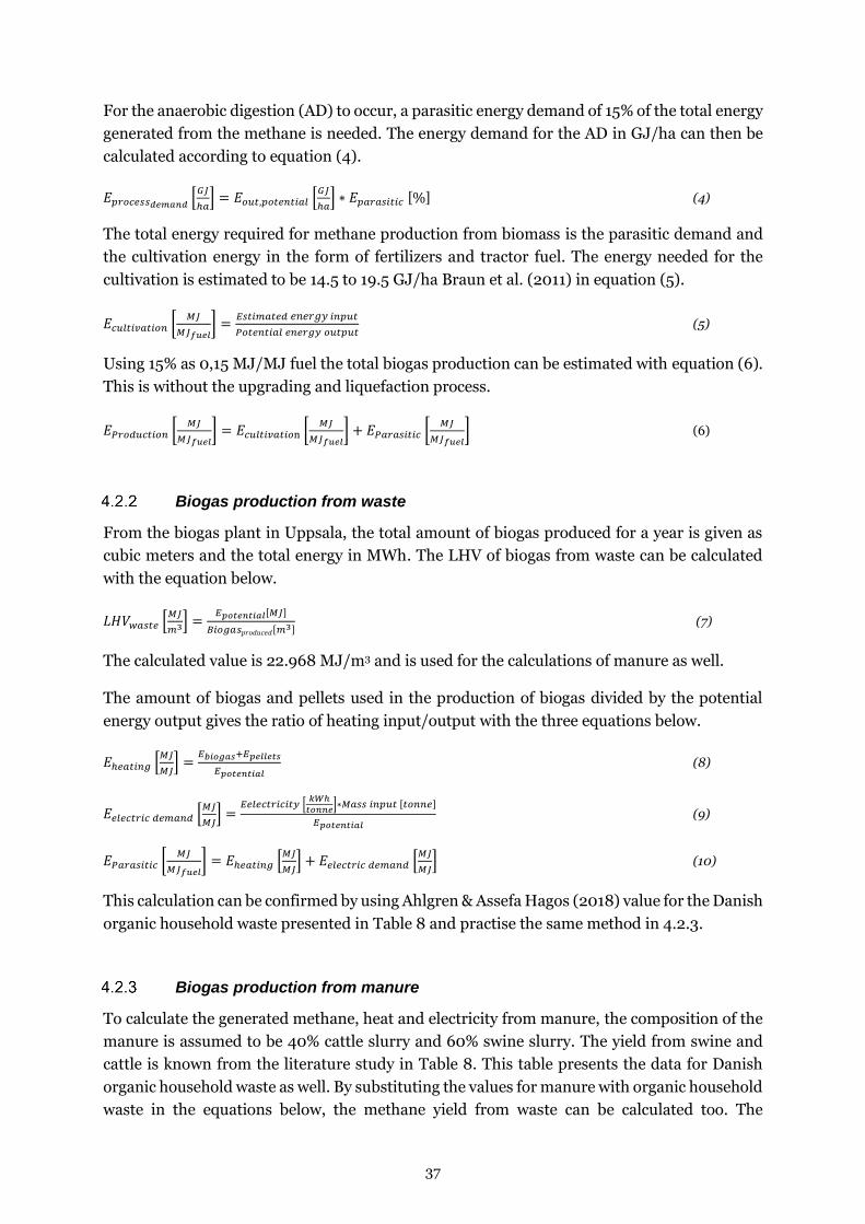
37

For the anaerobic digestion (AD) to occur, a parasitic energy demand of 15% of the total energy

generated from the methane is needed. The energy demand for the AD in GJ/ha can then be

calculated according to equation (4).

𝐸𝑝𝑟𝑜𝑐𝑒𝑠𝑠𝑑𝑒𝑚𝑎𝑛𝑑 [𝐺𝐽

ℎ𝑎] = 𝐸𝑜𝑢𝑡,𝑝𝑜𝑡𝑒𝑛𝑡𝑖𝑎𝑙 [

𝐺𝐽

ℎ𝑎] ∗ 𝐸𝑝𝑎𝑟𝑎𝑠𝑖𝑡𝑖𝑐 [%] (4)

The total energy required for methane production from biomass is the parasitic demand and

the cultivation energy in the form of fertilizers and tractor fuel. The energy needed for the

cultivation is estimated to be 14.5 to 19.5 GJ/ha Braun et al. (2011) in equation (5).

𝐸𝑐𝑢𝑙𝑡𝑖𝑣𝑎𝑡𝑖𝑜𝑛 [𝑀𝐽

𝑀𝐽𝑓𝑢𝑒𝑙] =

𝐸𝑠𝑡𝑖𝑚𝑎𝑡𝑒𝑑 𝑒𝑛𝑒𝑟𝑔𝑦 𝑖𝑛𝑝𝑢𝑡

𝑃𝑜𝑡𝑒𝑛𝑡𝑖𝑎𝑙 𝑒𝑛𝑒𝑟𝑔𝑦 𝑜𝑢𝑡𝑝𝑢𝑡 (5)

Using 15% as 0,15 MJ/MJ fuel the total biogas production can be estimated with equation (6).

This is without the upgrading and liquefaction process.

𝐸𝑃𝑟𝑜𝑑𝑢𝑐𝑡𝑖𝑜𝑛 [𝑀𝐽

𝑀𝐽𝑓𝑢𝑒𝑙] = 𝐸𝑐𝑢𝑙𝑡𝑖𝑣𝑎𝑡𝑖𝑜n [

𝑀𝐽

𝑀𝐽𝑓𝑢𝑒𝑙] + 𝐸𝑃𝑎𝑟𝑎𝑠𝑖𝑡𝑖𝑐 [

𝑀𝐽

𝑀𝐽𝑓𝑢𝑒𝑙] (6)

Biogas production from waste

From the biogas plant in Uppsala, the total amount of biogas produced for a year is given as

cubic meters and the total energy in MWh. The LHV of biogas from waste can be calculated

with the equation below.

𝐿𝐻𝑉𝑤𝑎𝑠𝑡𝑒 [𝑀𝐽

𝑚3] =

𝐸𝑝𝑜𝑡𝑒𝑛𝑡𝑖𝑎𝑙[𝑀𝐽]

𝐵𝑖𝑜𝑔𝑎𝑠𝑝𝑟𝑜𝑑𝑢𝑐𝑒𝑑[𝑚3]

(7)

The calculated value is 22.968 MJ/m3 and is used for the calculations of manure as well.

The amount of biogas and pellets used in the production of biogas divided by the potential

energy output gives the ratio of heating input/output with the three equations below.

𝐸ℎ𝑒𝑎𝑡𝑖𝑛𝑔 [𝑀𝐽

𝑀𝐽] =

𝐸𝑏𝑖𝑜𝑔𝑎𝑠+𝐸𝑝𝑒𝑙𝑙𝑒𝑡𝑠

𝐸𝑝𝑜𝑡𝑒𝑛𝑡𝑖𝑎𝑙 (8)

𝐸𝑒𝑙𝑒𝑐𝑡𝑟𝑖𝑐 𝑑𝑒𝑚𝑎𝑛𝑑 [𝑀𝐽

𝑀𝐽] =

𝐸𝑒𝑙𝑒𝑐𝑡𝑟𝑖𝑐𝑖𝑡𝑦 [𝑘𝑊ℎ

𝑡𝑜𝑛𝑛𝑒]∗𝑀𝑎𝑠𝑠 𝑖𝑛𝑝𝑢𝑡 [𝑡𝑜𝑛𝑛𝑒]

𝐸𝑝𝑜𝑡𝑒𝑛𝑡𝑖𝑎𝑙 (9)

𝐸𝑃𝑎𝑟𝑎𝑠𝑖𝑡𝑖𝑐 [𝑀𝐽

𝑀𝐽𝑓𝑢𝑒𝑙] = 𝐸ℎ𝑒𝑎𝑡𝑖𝑛𝑔 [

𝑀𝐽

𝑀𝐽] + 𝐸𝑒𝑙𝑒𝑐𝑡𝑟𝑖𝑐 𝑑𝑒𝑚𝑎𝑛𝑑 [

𝑀𝐽

𝑀𝐽] (10)

This calculation can be confirmed by using Ahlgren & Assefa Hagos (2018) value for the Danish

organic household waste presented in Table 8 and practise the same method in 4.2.3.

Biogas production from manure

To calculate the generated methane, heat and electricity from manure, the composition of the

manure is assumed to be 40% cattle slurry and 60% swine slurry. The yield from swine and

cattle is known from the literature study in Table 8. This table presents the data for Danish

organic household waste as well. By substituting the values for manure with organic household

waste in the equations below, the methane yield from waste can be calculated too. The

38

combined value for methane, heat and electricity generated is calculated with the three

following equations.

𝐶𝐻4𝑚𝑎𝑛𝑢𝑟𝑒 [𝑚3

𝑘𝑔𝐷𝑆] = %𝑠𝑤𝑖𝑛𝑒 𝑠𝑙𝑢𝑟𝑟𝑦 ∗ 𝐶𝐻4𝑦𝑖𝑒𝑙𝑑𝑠𝑤𝑖𝑛𝑒

[𝑚3

𝑘𝑔𝐷𝑆] + %𝑐𝑎𝑡𝑡𝑙𝑒 𝑠𝑙𝑢𝑟𝑟𝑦 ∗ 𝐶𝐻4𝑦𝑖𝑒𝑙𝑑𝑐𝑎𝑡𝑡𝑙𝑒

[𝑚3

𝑘𝑔𝐷𝑆] (11)

𝐻𝑒𝑎𝑡𝑚𝑎𝑛𝑢𝑟𝑒 [𝑀𝐽

𝑀𝐽𝑟𝑎𝑤𝑔𝑎𝑠] = %𝑠𝑤𝑖𝑛𝑒 𝑠𝑙𝑢𝑟𝑟𝑦 ∗ 𝐻𝑒𝑎𝑡𝑠𝑤𝑖𝑛𝑒 [

𝑀𝐽

𝑀𝐽𝑟𝑎𝑤𝑔𝑎𝑠] + %𝑐𝑎𝑡𝑡𝑙𝑒 𝑠𝑙𝑢𝑟𝑟𝑦 ∗ 𝐻𝑒𝑎𝑡𝑐𝑎𝑡𝑡𝑙𝑒 [

𝑀𝐽

𝑀𝐽𝑟𝑎𝑤𝑔𝑎𝑠] (12)

𝐸𝑙𝑒𝑐𝑡𝑟𝑖𝑐𝑖𝑡𝑦𝑚𝑎𝑛𝑢𝑟𝑒 [𝑀𝐽

𝑀𝐽𝑟𝑎𝑤𝑔𝑎𝑠] = %𝑠𝑤𝑖𝑛𝑒 𝑠𝑙𝑢𝑟𝑟𝑦 ∗ 𝐸𝑙𝑠𝑤𝑖𝑛𝑒 [

𝑀𝐽𝑒

𝑀𝐽𝑟𝑎𝑤𝑔𝑎𝑠] +%𝑐𝑎𝑡𝑡𝑙𝑒 𝑠𝑙𝑢𝑟𝑟𝑦 ∗ 𝐸𝑙𝑐𝑎𝑡𝑡𝑙𝑒 [

𝑀𝐽𝑒

𝑀𝐽𝑟𝑎𝑤𝑔𝑎𝑠] (13)

The potential energy from manure is calculated with the methane yield in m3 per tonne

multiplied with the LHV of methane in MJ/m3.

𝐸𝑝𝑜𝑡𝑒𝑛𝑡𝑖𝑎𝑙 [𝑀𝐽

𝑡𝑜𝑛𝑛𝑒] = 𝐶𝐻4𝑚𝑎𝑛𝑢𝑟𝑒 [

𝑚3

𝑡𝑜𝑛𝑛𝑒] ∗ 𝐿𝐻𝑉𝐶𝐻4 [

𝑀𝐽

𝑚3] (14)

The energy input to the manure (parasitic energy demand and CSTR) is calculated with the

potential energy out times the energy required for heat and electricity.

𝐸𝑖𝑛𝑚𝑎𝑛𝑢𝑟𝑒 [𝑀𝐽

𝑡𝑜𝑛𝑛𝑒] = 𝐸𝑝𝑜𝑡𝑒𝑛𝑡𝑖𝑎𝑙 ∗ (𝐻𝑒𝑎𝑡𝑚𝑎𝑛𝑢𝑟𝑒 + 𝐸𝑙𝑒𝑐𝑡𝑟𝑖𝑐𝑖𝑡𝑦𝑚𝑎𝑛𝑢𝑟𝑒) (15)

The parasitic energy demand for the biogas production is then calculated in equation (16).

𝐸𝑃𝑎𝑟𝑎𝑠𝑖𝑡𝑖𝑐 [𝑀𝐽

𝑀𝐽𝑓𝑢𝑒𝑙] =

𝐸𝑖𝑛𝑚𝑎𝑛𝑢𝑟𝑒[𝑀𝐽

𝑡𝑜𝑛𝑛𝑒]

𝐸𝑝𝑜𝑡𝑒𝑛𝑡𝑖𝑎𝑙[𝑀𝐽

𝑡𝑜𝑛𝑛𝑒] (16)

Liquefaction and upgrading

Ahlgren & Assefa Hagos (2018) estimates the upgrading process to require 0.2 to 0.3 kWh/m3

biogas and the liquefaction maximum energy demand to 1.56 kWh/kg LBG. These values have

been used for the liquefaction and upgrading process in all biogas cases. The equations used

are presented below.

The liquefaction energy required per MJ of fuel is given by dividing the liquefaction energy per

kg and the LHV of LBG as is presented in equation (17).

𝐸𝐿𝑖𝑞𝑢𝑒𝑓𝑎𝑐𝑡𝑖𝑜𝑛𝑓𝑟𝑎𝑐𝑡𝑖𝑜𝑛 [𝑀𝐽

𝑀𝐽𝑓𝑢𝑒𝑙] =

𝐸𝑙𝑖𝑞𝑢𝑒𝑓𝑎𝑐𝑡𝑖𝑜𝑛[𝑀𝐽

𝑘𝑔]

𝐿𝐻𝑉𝐿𝐵𝐺[𝑀𝐽

𝑘𝑔]

(17)

The energy required for upgrading per MJ of fuel is given by dividing the liquefaction energy

per m3 and the LHV of biogas as is shown in equation (18).

𝐸𝑖𝑛𝑢𝑝𝑔𝑟𝑎𝑑𝑖𝑛𝑔 [𝑀𝐽

𝑀𝐽𝑓𝑢𝑒𝑙] =

𝐸𝑢𝑝𝑔𝑟𝑎𝑑𝑖𝑛𝑔[𝑀𝐽

𝑚3]

𝐿𝐻𝑉𝐵𝐺[𝑀𝐽

𝑚3]

(18)

Tank-to-Wheels

In accordance with Scania, the data for the two reference vehicles are gathered from their

website at Scania (2019c). The vehicles are one diesel and one LNG truck, both with 410

horsepower and 13-litre engine. The torque for the LNG truck is 2000 Nm and for the diesel

39

truck 2150 Nm with both trucks having an engine power take-off (PTO) of 600 Nm. The weight

of the two trucks is assumed to be 39 tonnes payload.

Comparing different fuels by normal fuel consumption (FC) is not adequate when comparing

two different fuels. Therefore, the Tank-to-Wheels part will be calculated using the energy

content of the fuel consumed and compared in kg/100km. The FC for the vehicles has been

gathered in the literature study together with some data retrieved from Scania.

The combustion factor (CF) for LNG and diesel is given as g CO2/MJ and will be zero if the fuel

is renewable. The LHV for the fuel is given either as MJ/kg or MJ/m3. The emissions of N2O

and CH4 from the tailpipe are referred to as Exhaustemissions in the calculations and the unit is

g/kWhflywheel. The efficiency of the vehicles is given as a %. The values for each of these are

presented in Table 17.

Table 17 Data for TTW calculations used

Diesel LNG LBG

Combustion factor [g CO2eq/MJ] 73,8 56,2 0

LHV [MJ/kg] 43,1 45,1 45,1

N2O exhaust [g/kWh] 0,02 0,01 0,01

CH4 [g/kWh] 0 0,25 0,25

Efficiency [%] 44 40 40

The emissions from the combustion are calculated using the fuel consumption, the combustion

factor, and the heating value.

𝐶𝑜𝑚𝑏𝑢𝑠𝑡𝑖𝑜𝑛𝑒𝑚𝑖𝑠𝑠𝑖𝑜𝑛𝑠 [𝑘𝑔𝐶𝑂2𝑒𝑞

100𝑘𝑚] = 𝐹𝐶 ∗ 𝐶𝐹 ∗ 𝐿𝐻𝑉𝑓𝑢𝑒𝑙 (19)

The engine work is calculated with the knowledge of the FC, LHV and engine efficiency to be

able to estimate the amount of N2O and CH4 emitted.

𝑊𝑜𝑟𝑘𝑣𝑒ℎ𝑖𝑐𝑙𝑒 [𝑘𝑊ℎ

100𝑘𝑚] 𝑜𝑟 [

𝑀𝐽

100𝑘𝑚] = 𝐹𝐶 ∗ 𝐿𝐻𝑉𝑓𝑢𝑒𝑙 ∗ 𝜂𝑒𝑛𝑔𝑖𝑛𝑒 (20)

After the work is calculated, the emissions of N2O and CH4 can be calculated separately in CO2 equivalents as the GWP for each of them is known. The amount of the two molecules in the tailpipe emissions are given by thinkstep from the literature study in section 3.9.1.

𝐺𝐻𝐺𝑠𝑝𝑒𝑐𝑖𝑓𝑖𝑐 𝑒𝑚𝑖𝑠𝑠𝑖𝑜𝑛 [𝑘𝑔 𝐶𝑂2𝑒𝑞

100𝑘𝑚] = 𝑊𝑜𝑟𝑘𝑣𝑒ℎ𝑖𝑐𝑙𝑒 ∗ 𝐸𝑥ℎ𝑎𝑢𝑠𝑡𝑠𝑝𝑒𝑐𝑖𝑓𝑖𝑐 𝑒𝑚𝑖𝑠𝑠𝑖𝑜𝑛 ∗ 𝐺𝑊𝑃𝑠𝑝𝑒𝑐𝑖𝑓𝑖𝑐 𝑒𝑚𝑖𝑠𝑠𝑖𝑜𝑛 (21)

The complete emissions from the TTW are then calculated by adding the combustion emissions

with the CO2eq of N2O and CH4.

𝑇𝑇𝑊𝐺𝐻𝐺 [𝑘𝑔𝐶𝑂2𝑒𝑞

100𝑘𝑚] = 𝐶𝑜𝑚𝑏𝑢𝑠𝑡𝑖𝑜𝑛𝑒𝑚𝑖𝑠𝑠𝑖𝑜𝑛𝑠 + 𝑁2𝑂𝑒𝑚𝑖𝑠𝑠𝑖𝑜𝑛𝑠 + 𝐶𝐻4𝑒𝑚𝑖𝑠𝑠𝑖𝑜𝑛𝑠 (22)

The vehicles chosen is the Scania (2015) diesel vehicle and two different LNG vehicles. One

from thinkstep (2017) due to similar engine power and GTW and one from Unilever (2017)

due to the lower FC. The properties for the vehicles can be further studied in Table 18.

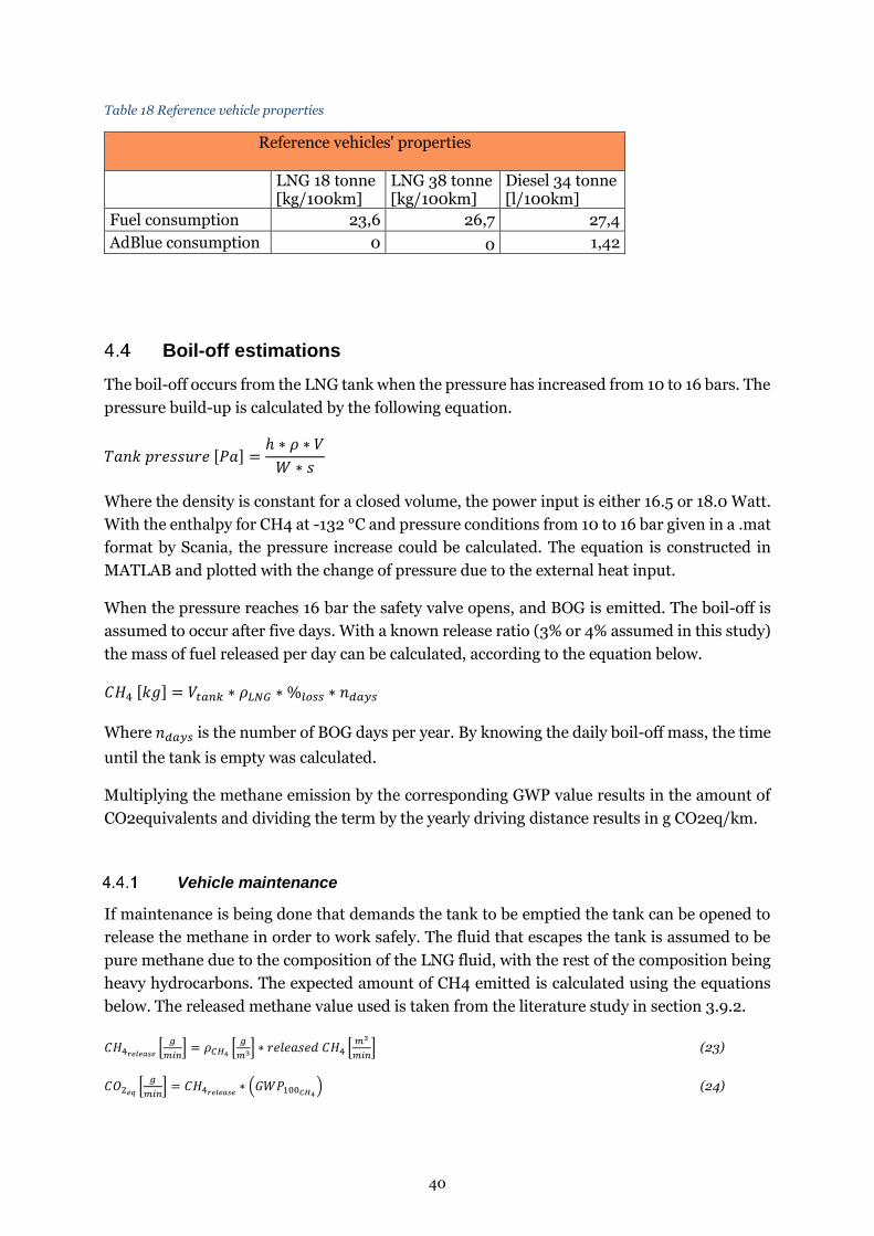
40

Table 18 Reference vehicle properties

Reference vehicles' properties

LNG 18 tonne [kg/100km]

LNG 38 tonne [kg/100km]

Diesel 34 tonne [l/100km]

Fuel consumption 23,6 26,7 27,4

AdBlue consumption 0 0 1,42

Boil-off estimations

The boil-off occurs from the LNG tank when the pressure has increased from 10 to 16 bars. The

pressure build-up is calculated by the following equation.

𝑇𝑎𝑛𝑘 𝑝𝑟𝑒𝑠𝑠𝑢𝑟𝑒 [𝑃𝑎] =ℎ ∗ 𝜌 ∗ 𝑉

𝑊 ∗ 𝑠

Where the density is constant for a closed volume, the power input is either 16.5 or 18.0 Watt.

With the enthalpy for CH4 at -132 °C and pressure conditions from 10 to 16 bar given in a .mat

format by Scania, the pressure increase could be calculated. The equation is constructed in

MATLAB and plotted with the change of pressure due to the external heat input.

When the pressure reaches 16 bar the safety valve opens, and BOG is emitted. The boil-off is

assumed to occur after five days. With a known release ratio (3% or 4% assumed in this study)

the mass of fuel released per day can be calculated, according to the equation below.

𝐶𝐻4 [𝑘𝑔] = 𝑉𝑡𝑎𝑛𝑘 ∗ 𝜌𝐿𝑁𝐺 ∗ %𝑙𝑜𝑠𝑠 ∗ 𝑛𝑑𝑎𝑦𝑠

Where 𝑛𝑑𝑎𝑦𝑠 is the number of BOG days per year. By knowing the daily boil-off mass, the time

until the tank is empty was calculated.

Multiplying the methane emission by the corresponding GWP value results in the amount of

CO2equivalents and dividing the term by the yearly driving distance results in g CO2eq/km.

Vehicle maintenance

If maintenance is being done that demands the tank to be emptied the tank can be opened to

release the methane in order to work safely. The fluid that escapes the tank is assumed to be

pure methane due to the composition of the LNG fluid, with the rest of the composition being

heavy hydrocarbons. The expected amount of CH4 emitted is calculated using the equations

below. The released methane value used is taken from the literature study in section 3.9.2.

𝐶𝐻4𝑟𝑒𝑙𝑒𝑎𝑠𝑒 [𝑔

𝑚𝑖𝑛] = 𝜌𝐶𝐻4 [

𝑔

𝑚3] ∗ 𝑟𝑒𝑙𝑒𝑎𝑠𝑒𝑑 𝐶𝐻4 [𝑚3

𝑚𝑖𝑛] (23)

𝐶𝑂2𝑒𝑞 [𝑔

𝑚𝑖𝑛] = 𝐶𝐻4𝑟𝑒𝑙𝑒𝑎𝑠𝑒 ∗ (𝐺𝑊𝑃100𝐶𝐻4) (24)

41

This maintenance procedure will not occur if the tank is filled more than half and from the

literature study it is estimated that 25% of the remaining 50% mass will escape during the

depressurization to ambient.

𝐹𝑢𝑒𝑙𝑙𝑒𝑣𝑒𝑙[𝑘𝑔] = 𝑀𝑎𝑥𝑡𝑎𝑛𝑘𝑙𝑒𝑣𝑒𝑙 ∗ 0,5 ∗ (1 − 0,25) − (𝐶𝑂2𝑒𝑞 ∗ 𝑇𝑖𝑚𝑒 [𝑚𝑖𝑛𝑢𝑡𝑒𝑠]) (25)

The approximated time for maintenance is not known, therefore a time step interval is used

for the calculations.

Particulates

Data received from Scania presents emissions by using PEMS to determine the exhaust

emissions. This data is excessive and no clear trend for PM or PN can easily be seen. The

measurements for LNG is still in an early stage which makes it even harder to find the relation.

Using CNG as fuel could be problematic due to the many combinations of compositions of the

gas.

Well-to-Wheels

To calculate the complete energy demand and GHG emissions for the WTW, the two following

equations are used. Where equation (26) is the case-specific WTT-value multiplied with the FC

and LHV of the specific fuel. The original WTT values do not account for the energy content in

the fuel, therefore, it is necessary with the addition of a one to the original value.

𝑊𝑇𝑊𝑒𝑛𝑒𝑟𝑔𝑦𝑓𝑢𝑒𝑙[𝑀𝐽

100𝑘𝑚] = (1 +𝑊𝑇𝑇𝑒𝑛𝑒𝑟𝑔𝑦𝑓𝑢𝑒𝑙 [

𝑀𝐽

𝑀𝐽𝑓𝑢𝑒𝑙]) ∗ 𝐹𝐶 ∗ 𝐿𝐻𝑉𝑓𝑢𝑒𝑙 (26)

As the final values for the GHG emissions have been calculated for both the WTT and TTW.

The WTW is a simple addition of the two values for each case and fuel.

𝑊𝑇𝑊𝐺𝐻𝐺𝑓𝑢𝑒𝑙 [𝑘𝑔 𝐶𝑂2𝑒𝑞

100𝑘𝑚] = 𝐹𝐶 ∗ 𝐿𝐻𝑉𝑓𝑢𝑒𝑙 ∗ 𝑊𝑇𝑇𝐺𝐻𝐺𝑝𝑟𝑜𝑑𝑢𝑐𝑡𝑖𝑜𝑛 [

𝑘𝑔 𝐶𝑂2𝑒𝑞

𝑀𝐽𝑓𝑢𝑒𝑙] + 𝑇𝑇𝑊𝐺𝐻𝐺𝑓𝑢𝑒𝑙 (27)

42

5 RESULTS

The result of the study is presented by dividing the Well-to-Wheels study into sections of WTT,

TTW, and WTW. An additional section is comparing the methane released during Boil-off and

maintenance.

Well-to-Tank results

The production paths for LNG both in terms of energy demand and CO2 equivalents are

presented in Table 19. The scenarios presented are created by using JEC values gathered in the

literature study with the main change in transportation method and distance. Other WTT

values used in the report or gathered in the literature study is presented in Appendix 1 and

used as verification. The final values of LBG from maize, manure, and waste are presented as

well as together with diesel.

When manure is used to produce LBG the production is actually considered to absorb CO2

instead of emitting. That is why the value in Table 19 is -9.498 g CO2eq/MJ when all other

sources have values above zero. The much lower value for manure (case 11) used as a reference

value from JEC (2014) has no specific fermentation process described.

Table 19 WTT scenarios LNG and LBG

WTT Data

Case

Description Final fuel

Energy input

[MJ/MJfuel]

Emissions [g

CO2eq/MJ ]

1 Produce->Liq at source->transport by ship->dist by truck->dispensing

LNG 0,2218 21,664

2 Produce->Liq at source->dist by truck->dispensing LNG 0,1267 14,208

3 Produce->transport pipeline 2500-Liq off source ->dist by truck->dispensing

LNG 0,1851 19,603

4 Produce->transport pipeline 4000-Liq off source ->dist by truck->dispensing

LNG 0,2290 22,597

5 Produce->transport pipeline 7000-Liq off source ->dist by truck->dispensing

LNG 0,3076 29,056

6 Produce->transport pipeline 2500-> dist by pipeline-> Liq off source ->dispensing

LNG 0,1735 15,580

7 On site liquefaction + 10 000km ship LNG 0,1800 19,906

8 Maize LBG 0,4709 41,202

9 Manure LBG 0,3005 -9,498

10 Waste LBG 0,3340 8,202

11 Manure (JEC, 2014) reference value LBG 2,054 -67,43

12 Diesel (pipeline) Diesel

0,204 15,435

13 Diesel (truck) Diesel 0,2163 18,864

43

The lowest value presented for LNG, both in terms of energy input and GHG is case 2. This

LNG is produced and liquefied at the source with a minimal transportation distance. The

highest value presented is correlated with the opposite, transportation by pipeline for 7000 km

before the liquefaction process and then distribution to the retail station. For all cases but

maize, using biomass as a source for the production of biogas results in higher energy demand

with lower GHG emissions compared with all LNG cases.

The share of each step in the WTT is presented in Figure 9. The transportation is highly

dependent on the path, and transformation is the major share for all cases except case 4 and 5.

Case 1 has a slightly higher transformation to and near market due to the loading and

unloading terminals for the ships. In case 1, 3, 4 and 5 the conditioning and distribution include

truck transport for 500km and dispensing at the retail station. Case 2 only have the retail

stations’ energy demand included in this value, as the transportation, in that case, is by the 500

km truck route. Case 6 has its distribution by pipeline. The two diesel cases only differ in the

distribution. The piped diesel has a slightly lower energy demand than the diesel distributed

by truck at 0.204 compared to 0.2163 MJ/MJ respectively.

Figure 9 WTT Energy input for different steps of the cases.

The GHG emissions for the WTT part given as g CO2eq/MJ are presented in Figure 10. Like

the energy demand in Figure 9, the main variable of the emissions is transportation. LNG 5

has the highest emissions both in both transportation and total emissions at 14.85 and 29.06

g CO2eq/MJ. The lowest emissions are from LNG 2 with a total amount of 14.21 g CO2eq/MJ.

For the two diesel cases, the piped diesel is slightly better at 15.44 g CO2eq/MJ compared to

the truck distributed diesel at 18.50 g CO2eq/MJ.

0,00

0,05

0,10

0,15

0,20

0,25

0,30

0,35

Diesel bypipe

Diesel bytruck

Case 1 Case 2 Case 3 Case 4 Case 5 Case 6 Case 7

Ener

gy in

pu

t [M

J/M

J]

Production Transformation at source Transportation to market

Transformation near market Conditioning & distribution

44

Figure 10 WTT GHG emissions g CO2eq/MJ

The WTT share for the LBG cases is presented in Figure 11. The major difference in the three

cases is the cultivation of maize which stands for roughly 0.136 MJ/MJ of the total 0.471

MJ/MJ. The other fuel does not have any cultivation. The transportation values are only for

distribution as it is assumed that there is no transportation included for gathering the manure

and waste. From an energy point-of-view, manure is the best choice of a resource for LBG

production, with an energy demand of 0.301 MJ/MJ.

Figure 11 WTT Energy input for different steps of the LBG cases.

0

5

10

15

20

25

30

35

Diesel pipe Diesel bytruck

Case 1 Case 2 Case 3 Case 4 Case 5 Case 6 Case 7

Emis

sio

ns

[gC

O2

eq/M

J]

Production Transformation at source Transportation to market

Transformation near market Conditioning & distribution

0,00

0,05

0,10

0,15

0,20

0,25

0,30

0,35

0,40

0,45

0,50

Maize Manure Waste

Ener

gy in

pu

t [M

J/M

J]

Cultivation Parasitic demand Upgrading

Liquefaction Road transport 500 KM Dispensing as LNG at retail site

45

In the GHG emission aspect, manure is still the lowest. In Figure 12 manure has negative GHG

emission while organic household waste is just above 8 g CO2eq/MJ. The only difference in

emissions is due to the parasitic demand.

Figure 12 WTT GHG emissions LBG

Sensitivity analysis

A sensitivity analysis of the complete production path is presented in Figure 13. It illustrates

that if diesel or LNG (1) is altered by ±10% in energy demand and emissions. The cases can be

better, equal or worse than each other. LNG ranges from 0.2-0.25 MJ/MJ and diesel from

0.18-0.22 MJ/MJ. Illustrated in the figure is that none of the biofuel cases will be equal or

better than the piped diesel or any LNG case except case 5. The wet manure case is JEC’s

reference case for LBG and is almost ten times higher than the best LBG case.

Figure 13 Sensitivity analysis of a 10% increase/decrease of the energy input per MJ.

-30

-20

-10

0

10

20

30

40

50

Cultivation Parasitic demand Upgrading LiquefactionRoad transport

500 KMDispensing as

LNG at retail site

Emis

sio

ns

[g C

O2

eq/M

J]

Maize Manure Waste

0,00

0,10

0,20

0,30

0,40

0,50

0,60

DieselPipe

DieselTruck

Case 1 Case 2 Case 3 Case 4 Case 5 Case 6 Case 7 Maize Manure Waste

Ener

gy in

pu

t [M

J/M

J]

Normal -10% 10%

46

In Figure 14 the sensitivity analysis of the cases illustrates that case 2 and 6 are the only LNG

cases that can have fewer emissions than the piped diesel case. The best case of all is manure

where CO2 is being absorbed.

Figure 14 Sensitivity analysis of a 10% increase/decrease of emissions in CO2 equivalents per MJ.

The energy required for transportation by pipeline in different distances and by shipping from

JEC is used to find the intersection point. Average values for pipeline transportation are used

together with linear interpolation. As can be seen in Figure 15, the transportation of gas by

pipeline requires more energy if the distance is higher than 1404 km.

Figure 15 Energy demand as a function of the distance for transportation in the pipeline and by ship

-20

-10

0

10

20

30

40

50

DieselPipe

DieselTruck

Case 1 Case 2 Case 3 Case 4 Case 5 Case 6 Case 7 Maize Manure Waste

Emis

sio

ns

[g C

O2

eq/M

J]

Normal -10% 10%

0

0,05

0,1

0,15

0,2

0,25

0,3

0,35

0,4

0 1000 2000 3000 4000 5000 6000 7000 8000 9000 10000

Ener

gy in

pu

t [M

J/M

J]

km

MJ/MJ Pipeline MJ/MJ Shipping

47

The CO2 emissions corresponding to transportation has a similar trend as the energy demand.

The intersection for the two transportation methods occurs at 1550 km which is slightly earlier

than for the energy demand. Average values have been used for the emissions from the

different pipeline distances because they are not fully linear. The intersection point can be

further studied in Figure 16.

Figure 16 g CO2eq/MJ as a function of the distance for transportation by pipeline and by ship

Tank-to-Wheels results

The Tank-to-Wheels results are divided by energy demand and GHG emissions. This includes

the WTT section according to the fuel consumption of the vehicles.

Energy demand

Using the reference fuel consumption of 26.7 kg/100km and a flywheel efficiency of 36%, the

energy input is calculated to be approximately 1200 MJ/100km presented in Table 20. This is

with a heating value of 45.1 MJ/kg, the European standard value.

Table 20 LNG TTW energy result

LNG TTW ENERGY

Fuel Consumption [kg/100km] 26,7

Efficiency 0,361

Energy input [MJ/100km] 1204,17

Diesel is having a higher efficiency compared to LNG together with a lower heating value as

well as fuel consumption. Even though AdBlue requires high energy input in the production

process the sum of the two is significantly lower than for the LNG vehicle in terms of energy

input. The values are given in Table 21.

0

5

10

15

20

25

30

35

0 1000 2000 3000 4000 5000 6000 7000 8000 9000 10000

Emis

sio

ns

[g C

O2

eq/M

J]

km

g CO2eq/MJ Pipeline g CO2eq/MJ Shipping

48

Table 21 Diesel TTW energy result

DIESEL TTW ENERGY

Fuel Consumption [kg/100km] 22,797

Efficiency 0,440

Energy input [MJ/100km] 982,542

Engine work output [kWh/100km] 120,088

AdBlue energy input [MJ/100km] 14,075

Total energy demand [MJ/100km] 996,617

Greenhouse gas emissions

The emission factors used for the calculation of the TTW emissions in GHGs are presented in

Table 22.

Table 22 Values used for TTW GHG emissions

Diesel LNG LBG

Combustion factor [g CO2eq/MJ] 73,8 56,2 0

LHV [MJ/kg] 43,1 45,1 45,1

N2O exhaust [g/kWh] 0,02 0,01 0,01

CH4 exhaust [g/kWh] 0 0,25 0,25

With a fuel consumption of 26.7 kg/100km the LNG is producing a total of almost 72 kg CO2

equivalents with the majority of the emissions in direct CO2 as presented in Figure 17. Even

though the diesel truck has zero emissions in the form of CH4, the combustion factor for diesel

is significantly higher resulting in almost 5kg more CO2 equivalents/100 km.

The emissions from AdBlue in the diesel truck and the methane emissions from the LNG truck

are equal in CO2 equivalents. The N2O emissions from the diesel truck are 0.8 kg CO2eq/100km

and from the LNG truck, 0.5 kg CO2eq/100km. As the combustion of biofuels has a combustion

factor of 0, the emissions from the LBG are only 0.5 kg CO2eq/100km in from N2O. Having a

higher emission factor results in CO2 emission of almost 5kg equivalents per 100 km.

Figure 17 TTW emissions of CO2 equivalents per 100km.

0

10

20

30

40

50

60

70

80

90

Diesel LNG LBG

Emis

sio

ns

[kg

CO

2eq

/10

0km

]

CO2 from combustion CH4 N2O AdBlue GHG

49

From the emissions factors given by Transportstyrelsen for the reference vehicles, the total

emissions of carbon monoxide (CO), total hydrocarbons (THC), noxious oxide (NOx) and

particulates are presented in Table 23. The LNG truck has the highest emissions of CO with

41.96 g/100km and the diesel truck has the highest emissions of NOx with 46.49 g/100km.

Table 23 Emissions per 100km for the reference vehicles.

Emissions from reference vehicles Diesel 44% Efficiency

LNG 40% Efficiency

CO [g/100km] 3,39 41,96

THC [g/100km] 1,09 -

NOx [g/100km] 46,49 21,18

Particulates [g/100km] 0,31 0,31

Sensitivity analysis Diesel engine efficiency

The diesel case presented in the sensitivity analysis is the case with distribution by pipeline

and the engine efficiency taken from the literature study. The efficiency is strongly correlated

with the fuel consumption and therefore a sensitivity analysis represents the difference in

Table 24. The amount of CO2 emission is reduced by more than 15 kg/100 km between the

best and worst scenarios. The emissions of N2O are directly correlated to the work, so the

emissions per 100km are the same, but less fuel is used to reach 100 km, therefore also

reducing the total N2O emissions.

Table 24 Diesel efficiency sensitivity analysis for GHG emissions

Vehicle efficiency effect on emissions and fuel consumption

Efficiency [%] 0,36 0,38 0,4 0,42 0,44

Fuel consumption [kg/100km] 22 21 20 19 18

Work [kWh/100km] 94,82 95,54 95,78 95,54 94,82

N2O [kg CO2eq/100km] 0,65 0,65 0,66 0,65 0,65

TTW diesel [kg CO2eq/100km] 70,01 66,83 63,64 60,46 57,28

WTT Diesel [kg CO2eq/100km] 14,64 13,97 13,31 12,64 11,97

AdBlue consumption [kg/100km] 1,49 1,43 1,36 1,29 1,22

TTW Diesel [kg CO2eq/100km] 70,66 67,48 64,30 61,12 57,93

WTW Diesel [kg CO2eq/100km] 85,29 81,45 77,61 73,76 69,90

50

Similar to the GHG emissions, the energy demand is reduced by 200 MJ/100km presented in

Table 25. This result also shows that the worst case for diesel, 1 141.82 MJ/100km is still lower

than the results seen in Table 20 for LNG.

Table 25 Diesel efficiency sensitivity analysis for energy demand

Vehicle efficiency effect on energy demand and fuel consumption

Efficiency [-] 0,36 0,38 0,4 0,42 0,44

Fuel consumption [kg/100km] 22 21 20 19 18

Work [kWh/100km] 94,82 95,54 95,78 95,54 94,82

WTW AdBlue Energy [MJ/100km] 13,58 12,97 12,66 11,73 11,11

WTW Diesel [MJ/100km] 1 141,82 1 089,92 1 063,97 986,12 934,22

Boil-off results

The boil-off consists of two steps, the initial step is the pressure build-up which represents the

time it takes until the pressure reaches 16 bar. The time depends on the heat input from the

surrounding. The second step is when the safety valve breaks at 16 bar and the methane is

released.

Figure 18 illustrates the difference when boil-off occurs corresponding to different heat inputs

and fuel levels. If the heat input is 16.5 W and the tank is full when a standstill happens, the

pressure will reach 16 bar after roughly 7.5 days and then boil-off follows. For 18 W heat input

and full tank the boil-off starts after 7 days. If the tank is half-full during standstill, it takes

almost 5 and 4.5 days for boil-off to occur for a heat input of 16.5 W and 18 W respectively.

Figure 18 Pressure build-up in an LNG tank with a heat input of 16.5 and 18 W.

0%

10%

20%

30%

40%

50%

60%

70%

80%

90%

100%

110%

0 1 2 3 4 5 6 7 8

Star

tin

g vo

lum

e

Number of days

18

16,5

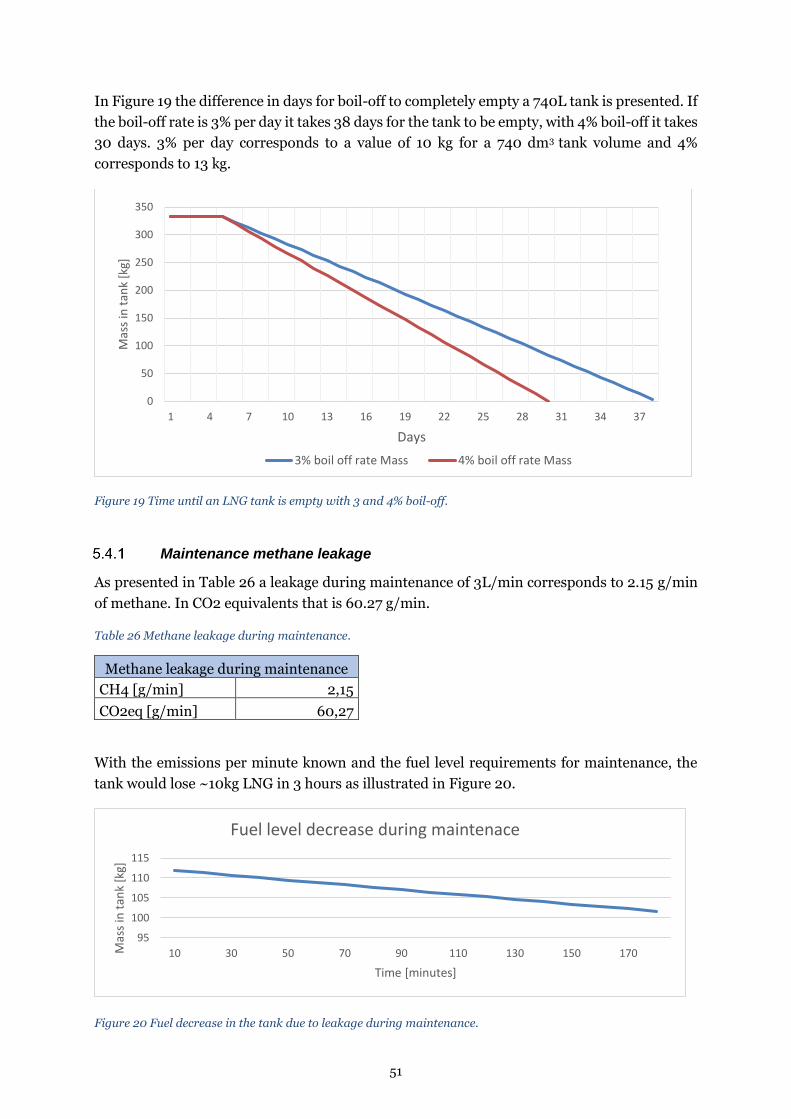
51

In Figure 19 the difference in days for boil-off to completely empty a 740L tank is presented. If

the boil-off rate is 3% per day it takes 38 days for the tank to be empty, with 4% boil-off it takes

30 days. 3% per day corresponds to a value of 10 kg for a 740 dm3 tank volume and 4%

corresponds to 13 kg.

Figure 19 Time until an LNG tank is empty with 3 and 4% boil-off.

Maintenance methane leakage

As presented in Table 26 a leakage during maintenance of 3L/min corresponds to 2.15 g/min

of methane. In CO2 equivalents that is 60.27 g/min.

Table 26 Methane leakage during maintenance.

Methane leakage during maintenance

CH4 [g/min] 2,15

CO2eq [g/min] 60,27

With the emissions per minute known and the fuel level requirements for maintenance, the

tank would lose ~10kg LNG in 3 hours as illustrated in Figure 20.

Figure 20 Fuel decrease in the tank due to leakage during maintenance.

0

50

100

150

200

250

300

350

1 4 7 10 13 16 19 22 25 28 31 34 37

Mas

s in

tan

k [k

g]

Days

3% boil off rate Mass 4% boil off rate Mass

95

100

105

110

115

10 30 50 70 90 110 130 150 170Mas

s in

tan

k [k

g]

Time [minutes]

Fuel level decrease during maintenace

52

Well-to-Wheels results

The total energy demand per 100km for all the fuels is presented in Figure 21. What can be

seen is that there is just LNG case 2 with a fuel consumption of 23.6 kg/100km that has as low

energy demand as the two diesel cases. The energy demand for the two diesel cases is roughly

1200 MJ/100km. The other LNG cases range from 1357-1575 MJ/100km. The lowest energy

demand for the three LBG sources is from manure which has a demand of 1566 MJ/100km.

Maize has the highest energy demand at 1771 MJ/100km and waste has a demand of 1606

MJ/100km.

Figure 21 Complete WTW energy demand in MJ/100 km.

The GHG emissions in kg CO2eq/100km are presented in Figure 22. In the figure, the fuel

consumption for all LNG cases is 26.7 kg/100km except for another case 2 with a fuel

consumption of 23.6 kg/100km. The flywheel efficiency for the diesel truck is 44% and for the

gas truck 40%. The boil-off is 3 wt% per day with a duration of three days and the driving

distance is 120 000 km a year. The distance and conditions are the same Iveco used.

Illustrated in Figure 22, producing LBG from manure, the GHG emissions are - 11.44

compared to the 49.61 kg CO2eq/100km of maize. This is even higher than the worst case of

LNG, namely case 5 at 34.99 kg CO2eq/100km. As previously stated, the combustion of biofuels

has 0 GHG emissions while the combustion of LNG yields 67.71 kg CO2eq/100km with a fuel

consumption of 26.7 kg/100km and 59.85 kg CO2eq/100km for a fuel consumption of 23.6

kg/100km.

The biggest contributing factor to GHG emissions from a diesel WTW is the combustion of the

fuel in the vehicle, representing roughly 80% of the total emissions. The same is true for LNG

with the combustion being the major emissions contributor. The piped diesel WTW has a final

value of 89.0 kg CO2eq/10okm and the truck distributed diesel case 92.01 kg CO2eq/10okm,

0

200

400

600

800

1000

1200

1400

1600

1800

Ener

gy d

eman

d [

MJ/

10

0 k

m]

Energy demand MJ/100 km AdBlue

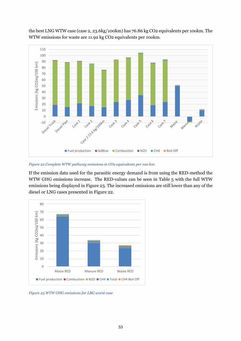
53

the best LNG WTW case (case 2, 23.6kg/100km) has 76.86 kg CO2 equivalents per 10okm. The

WTW emissions for waste are 11.92 kg CO2 equivalents per 10okm.

Figure 22 Complete WTW pathway emissions in CO2 equivalents per 100 km.

If the emission data used for the parasitic energy demand is from using the RED-method the

WTW GHG emissions increase. The RED-values can be seen in Table 5 with the full WTW

emissions being displayed in Figure 23. The increased emissions are still lower than any of the

diesel or LNG cases presented in Figure 22.

Figure 23 WTW GHG emissions for LBG worst case

-10

0

10

20

30

40

50

60

70

80

90

100

110

Emis

sio

ns

[kg

CO

2eq

/10

0 k

m]

Fuel production AdBlue Combustion N2O CH4 Boil-Off

0

10

20

30

40

50

60

70

80

Maize RED Manure RED Waste RED

Emis

sio

ns

[kg

CO

2eq

/10

0 k

m]

Fuel production Combustion N2O CH4 Total CH4 Boil Off

54

The result of a boil-off rate increase from 3% to 4% for LNG 2 with a fuel consumption of 26.7

kg/100km is illustrated in Figure 24. The boil-off share then represents 1.07% of the total

emissions. A 30-minute yearly maintenance results in 0.0015% of the total emissions/100 km.

Figure 24 WTW emissions per 100km in percentage including a boil-off rate of 4% and maintenance for GWP100.

A sensitivity analysis was performed for the effect of changing the GWP value from the GWP100

to the GWP20 values presented in section 3.9. With a higher GWP for methane, the share of

fuel production emissions increase from 19.64% to 30.98%. The fuel combustion emissions

decrease from 77.74% to 63.60% and the N2O emissions from 0.57% to 0.41%. Boil-off and

maintenance emissions increase from 1.07% to 2.63%.

Figure 25 WTW emissions per 100km in percentage including a boil-off rate of 4% and maintenance for GWP20.

Fuel production19,64%

Combustion77,74%

N2O0,57%

CH40,97%

1% BOG0,27%

3% BOG0,80%

Maintenance0,00%

Other1,07%

Fuel production Combustion N2O CH4 1% BOG 3% BOG Maintenance

Fuel production30,98%

Combustion63,60%

N2O0,41%

CH42,38%

1% BOG0,66%

3% BOG1,97%

Maintenance0,00%

Other2,63%

Fuel production Combustion N2O CH4 1% BOG 3% BOG Maintenance

55

6 DISCUSSION

The discussion is divided into three sections, Well-to-Tank, Tank-to-Wheels, and Well-to-

Wheels and their corresponding subsections. The discussion chapter covers the information

gathered in the literature study and the presented results.

Well-to-Tank discussion

In the Well-to-Tank section, the fuel properties, production, processing, transportation, and

distribution will be discussed.

The main factors contributing to the energy input and emissions in our work are the

transportation distances and method. This is mainly for the reason that the same value has

been used for production and processing. Small changes were done for the conditioning and

distribution part as well.

The values in the production of NG comes from an average of JEC’s production and processing

values. Changing the WTT values with 10%, both up and down, showed that the difference for

the different fuels is very low. Which of the fuels that are considered to be the best or having

the lowest GHG emissions are very sensitive to changes. If the production of diesel is 10%

worse than the reference value many of the LNG cases is suddenly better.

Fuel properties

The heating value of natural gas and LNG differ depending on the main source. Using a gas

produced in Europe will have a different composition and heating value compared with gas

produced in Russia. This is not a major difference for the LNG, even though, if compared to

LBG the methane number varies some. For LNG, the average European heating value is used,

this is slightly lower than the Russian mix. Using a lower heating value gives the European

LNG an advantage related to the energy demand for the combustion if compared with the same

fuel consumption. This is true if the fuel consumption is the same for the two cases. In reality,

the fuel consumption should be dependent on the heating value and therefore the efficiency as

well. With a higher heating value, less fuel should be used to attain the same work. Little

information is given in this aspect and the fuel consumption found does not cover what origin

the fuel has. Even for diesel, the literature study showed different heating values depending on

the source.

The correlation between methane number and Wobbe index, and, the impact it has on the

operating conditions for an engine have not been taken into account for the energy demand. If

the Wobbe index is low, there is a higher risk of knock in the engine which would affect the

injection and ignition of the fuel. Until there are clear regulations for gas quality in the grid,

engine manufacturers can’t optimize their engines for a lower range of fuel quality. This mostly

affects CNG, but there is scarce information about the impact of quality on LNG. Due to the

56

lack of data in this area, no assumptions could be made, and it has not been taken into account

for our calculations.

The density of LNG and LBG used in the degree project is assumed to 450 kg/m3 which is an

assumption from the data given by several different sources. These sources have variations

from 410-500 kg/m3 and no clearly stated pressures, temperatures or compositions. This

leaves the uncertainty of the LNG estimations and calculations at a greater scale than for diesel.

Furthermore, the vehicle manufacturer uses different temperatures for the LNG in the tank

which increases the difficulty of determining a general value for the density. In the calculations

made the density affects the total mass in the tank and therefore only the capacity and amount

of BOG.

Fuel production

The emissions and energy from extraction and pre-processing of oil and natural gas have a

high risk of being biased. The concerned actors of the market want to retain their business in

a world with more interest and demands on the environmental impact. In terms of the

production for diesel, JEC is the most referenced source found in the literature study. This is

concerning due to the work only having one reference value for diesel while including several

cases for NG. NG and diesel are extracted from the same source and should, therefore, have a

similar amount of cases, both for refining and transportation. The production and processing

value received from JEC for NG includes, as the name suggests, both the production and

processing. Using the pure NG directly in a liquefaction plant should in theory not need the

initial pre-processing step and therefore have a lower energy value than stated.

The data from production sites is scarce which results in a low possibility to validate the actual

emissions during the operation. thinkstep uses data received from actual plants and mainly

refers to the Norwegian sites. Norway has under a long period of time focused on reducing the

emissions during natural gas and crude oil operations. Therefore, these figures might not

represent the average oil and gas production site. The report from T&E refers to the work done

by Exergia. Exergia states that the losses and GHG emissions are much higher in the

production path compared to JEC and thinkstep’s result. That is most likely due to the

inconsistent data of emissions from the production sites.

Besides the diesel in the production path, AdBlue is consumed as well in Euro VI classified

vehicles. The data used for the production and correlated emissions are gathered from a report

based on production in New Zealand. This value might be different if the ammonia production

should occur in another geographical location. This was not further studied due to the low

amount used in the diesel vehicle. Even though ammonia, which is part of AdBlue, is highly

energy demanding in the production process.

Using manure as the main substrate in biogas production causes the GHG emissions to be

negative. This is due to the prevention of methane to spontaneously emit to the atmosphere if

it is not collected. The emissions are then highly affected by the temperature and geographical

location of where the manure is retrieved, as a higher temperature yields more emissions. The

low value from JEC in this aspect is hard to validate. The emissions used in this work is the

Swedish average. Producing manure further south might result in a higher negative number

57

similar to JEC’s result, this assuming the increase is similar to the values in Table 9. JEC does

not specify the fermentation process and therefore is difficult to verify.

Different crops require certain soils, climate, and fertilizers from one another. Therefore, local

agriculture and biogas producers can have profitable collaborations as digestate from biogas

production often can be utilized as fertilizers for crops or feed for livestock. Manure from e.g.

swine farms can be used to produce biogas. The possible yield from different substrates is also

a large factor if a crop is better suited for biogas production or food. Or if another crop should

be produced instead.

Depending on if the electricity produced for the biogas plant is from fossil or renewable sources

have a great impact on whether or not the production emissions are low or high. From

renewable sources, the emissions during the combustion are considered to be zero, as the

source is assumed to absorb CO2 during cultivation. This creates a bit of uncertainty when it

comes to waste, should waste be considered renewable and have a CO2 neutral impact in the

combustion? The production and origin of the waste are more often than not unknown. Based

on the available knowledge and assumptions on this matter, waste is today deemed as

renewable in this aspect. If the electricity is produced in a combined heat and power plants

(CHP), the energy demand for the electricity is increased while the emissions are lowered.

Normally for the extraction of crude, fossil fuels are used to power the production site. For

biogas plants, it is renewable biogas that is used instead. The greatest difficulty is to value the

higher energy input using renewables with the lower energy input using fossil fuels. Having

significantly lower GHG emissions and with renewable energy sources, in theory, are unlimited

the amount of energy input is irrelevant. For the renewable energy source to be weighed against

a fossil-based PES, other factors need to be added. This might be in terms of land use, the fact

that biomass in the forms this work has presented cannot be used unlimited or other aspects.

Fuel processing

The emissions associated with processing gas is dependent on the primary energy source used.

In a country with a high ratio of renewable sources in electricity production, GHG emissions

are lower compared with a country using a high amount of fossil fuel. The energy required for

processing is different due to the method used. Though, for comparability purposes, the values

from JEC are used due to their combined production and processing methods. This is the

reason for the biogas being upgraded to bio-methane as well as being liquefied. This results in

a slightly higher value than needed, as processing is not necessary for LBG production. The

liquefaction values used for LNG is taken from JEC while the values for LBG is taken from the

study made by Ahlgren & Assefa Hagos. This is to include the possibility of higher energy

demand for local small-scale liquefaction plants.

Transportation and distribution

As can be seen in the result the energy and emissions correlated to the transport of LNG are

increasing with the distance. Increasing the pipeline length demands additional electricity to

power the pumps to keep the pressure. Another aspect related to increased pipeline length is

58

the additional methane emissions occurring as there are more connections and sources of

leakage. As methane is having a high GWP value this affects the GHG emissions even more.

Normally long-distance transportation of fuel is done using large carrier ships. This is done for

the diesel case as well as for two of the LNG cases presented, cases 1 and 7. The diesel value

related to transportation is more than 7 times lower compared with the similar LNG

transportation presented by JEC. In the study made by thinkstep, a set of ships using different

technologies were presented with none of them having as high values as the one used by JEC.

Case 7 is, therefore, the values from JEC in all aspects besides the transportation value. One of

the reasons for the low diesel transportation value could be that diesel is being transported in

larger volumes.

When it comes to the emissions and energy demand from transportation, it might be more

suitable to have shorter ranges on transportation. However, that could, in turn, limit the

possibilities of utilizing different fuels in certain locations. Moreover, depending on the

production method used, a longer transportation distance might reduce the overall emissions.

This is if the method of production is increasingly efficient at reducing emissions. The major

source for the high emissions correlated with the transportation using pipelines is the methane

slip. If this could be avoided, then the pipeline method could be more environmentally friendly.

For organic household waste and manure, no initial transportation to the biogas plant is

accounted for. As it is assumed that it must be collected either way. For maize, the assumption

is that the biogas plant is positioned close to the cultivation site. Therefore, no additional

transportation is accounted for either. However, the energy needed for fertilizers and tractor

operation has been included. The distribution truck is assumed to have a travel distance of

500km no matter what fuel it will deliver. Maybe this should vary as biogas plants usually are

located closer to the retail stations it will be distributed to. As the production volume of biogas

is much lower than for LNG and diesel. On the contrary, a distribution distance of more than

500km might feel a bit too extensive, and just the most rural retailers will be farther away than

500km. So, even though the distribution distance might be a bit high, it will include more

actual routes than if it would be shorter.

The second case for diesel had increased GHG emissions due to the more energy demanding

distribution process. This is the same distribution used for almost all LNG cases and the change

is to compare the fuels in a fair way.

Tank-to-Wheels discussion

Different factors concerning the TTW will be presented below. This includes fuel consumption,

emissions of GHGs and particulates as well as BOG and maintenance emissions.

Fuel consumption

The fuel consumption together with the flywheel efficiency for the vehicles are the main factors

in both energy demand and GHG emissions. Previous research compares the fuels in kg/100

km and l/100 km respectively for LNG and diesel which results in higher fuel consumption for

59

diesel. Furthermore, having different temperatures in the LNG tank results in different density

and therefore fuel capacity. As mentioned in the Fuel production section this affects the

properties of the fuel and results in some uncertainties.

It is important to notice that the heating value varies on weight and volume basis depending

on the density of the fuel. That is why it is important to find a comparison where the fuels are

being matched in a fair way. We found that weight basis was the most objective assessment in

this study.

In the study made by thinkstep the fuel consumption used was 26.7 kg/100 km for LNG and

31.5 litres/100 km for diesel. This resulted in very similar fuel consumptions in kg/100 km.

However, with different characteristics of the diesel and Otto engine, the fuel consumption is

higher for an Otto engine, which is applied in this study. Using the same fuel consumption

would be an unfair method of comparison, as the vehicles and engines today will have different

fuel consumptions depending on the fuel. Therefore, data were collected from both Iveco and

Scania for fuel consumption and engine efficiency.

The two fuel consumptions used for LNG are gathered from public documentation and might

not be the latest figures the manufacturers have. However, for comparison, these values are

still relevant as a trend can be seen with a lower FC.

Emissions and particulates

In previous work done by TNO it is stated that PEMS has low accuracy. Therefore, accurate

measurements are hard to find for the number of particulates from the combustion of the

different fuels. The data gathered from Scania could not be used to compare different fuels due

to different measuring methods and no clear trend. The amount of data that represented LNG

emissions were scarce and could not be used to find a general connection with the emissions

from the diesel vehicle. The actual vehicles’ registration number was used to find the emissions

from Transportstyrelsen. This information does not correspond to all possible emissions and

therefore the same estimation used by thinkstep for N2O and CH4 is applied. Though, the

values from Transportstyrelsen states that there are no THC emissions for the LNG vehicle

during the WHTC which should mean that there are no methane emissions. Scania, on the

other hand, is using their own standard values which results in a higher N2O emission and a

lower CH4 emission compared to thinkstep. This method does not have any public references

that can be used to estimate the emissions, using that would limit the reliability in the work.

Comparing the data gathered from Transportstyrelsen results in similar emissions in

particulates though it does not state the particulate size. Micro-particulates have a larger

impact on human health and would, therefore, be worse if it is present on a larger scale in any

of the fuels.

When it comes to particulates, the regulation of PN was first introduced in the Euro VI

standards. Whereas the testing conditions and equipment for the measurements still hasn’t

been completely determined. This is a cause of uncertainty over the few available figures

concerning PN emissions, therefore, it is was excluded in the result of this study. The

measuring of PM is still also highly ambiguous and the PEMS is unreliable, therefore the

60

HWTC values given by Transportstyrelsen was used to calculate the probable particulate

emissions per 100km.

N2O should probably be reduced with a lower fuel consumption even though the efficiency is

increasing. This might be a flaw in the method used to calculate the exhaust emissions. The

same should be valid for LNG as well. However, the method was not evaluated further and

stood as it is. Even though the values might not be completely correct as a consequence of this,

emissions from both the vehicles are calculated using the same method. Changing the number

of emissions from the vehicle had to be increased excessively for any significant changes to

occur.

The assessment is conducted by using the most recent GWP values for CH4 and N2O presented

by IPCC in their AR5 report. Therefore, the emissions in this study are higher compared to the

values presented by JEC (2014) where the AR4 values are used.

The combustion factor used in this work and stated by IPCC assumes stoichiometric

combustion. This is solved by adding exhaust gases in the form of CH4 and N2O using a

percentage of the Euro VI limit. Thus, adding additional emissions. This means that the

emissions presented in the results are higher in terms of CO2 than they should.

Boil-off and maintenance

The boil-off from the LNG vehicle is hard to estimate, especially when it should not occur under

normal use of the truck. To estimate the impact of the boil-off, two scenarios were created to

compare the results. Previous research has stated that the boil-off is insignificant compared

with the rest of the emissions. Therefore, the cases use both 3% and 4% of the mass for daily

boil-off for three days. Worth knowing is that the vehicle must be stationary for at least 5 days

prior to the actual boil-off period for the pressure to build up. To add additional potential

emissions in the form of methane a case which includes maintenance of the vehicle is made.

This is done to compare the number of losses due to lowering the pressure and opening of the

tank. This type of maintenance does not occur too frequently and is added as the worst type of

scenario. Including both the boil-off and the maintenance, the combined impact of this BOG is

around 1% of total emissions. Therefore, it is almost completely negligible.

During maintenance, only the assumption of a 3L/min flow from the tank is used. This is due

to the lower density of methane compared to air. There have been no calculations of this

estimation and therefore the value might be different. Furthermore, has the maintenance

duration been assumed to be 30 minutes during the cases and that 25% of the total mass

escapes during the depressurization.

As there is no available data on how much methane is released to the atmosphere during

refuelling. This is not taken into consideration in this study. From discussions with employees

at Scania, these emissions are most likely negligible and could be included in the BOG from

standstill and maintenance.

61

Well-to-Wheels discussion

As previously mentioned in the Fuel consumption section, the fuels in this study have been

compared on a weight basis as it felt as the most fair assessment. The energy demand is

evaluated in MJ/MJfuel and the emissions on g CO2 equivalents. This made the comparisons

clear, structured and offers a good overview.

The best case for LNG, where the gas is locally produced, liquefied and distributed to a retailer,

is better than the diesel case where the fuel consumption is similar. The diesel fuel is, on the

other hand, transported 10 000 km in that scenario compared to the LNG transportation

distance of 500 km. When the LNG truck with the lower FC is compared with the standard

diesel case, the emissions from the LNG truck are significantly lower. The only fuel to have

overall negative GHG emissions is LBG from manure. This is largely due to the combustion

being CO2 neutral. And that the production of biogas from manure has a great impact on

reducing GHG emissions as the emissions value is negative and seen as absorbing CO2.

There are higher NOx emissions from diesel compared to the LNG truck, this is because of a

deficit of oxygen in the combustion. On the other hand, there is an excess of oxygen in the LNG

combustion so the CO emissions are higher than for diesel. Though, the amount of N2O in the

NOx is not stated therefore no actual conclusion can be drawn from this.

As presented in 1.1.2 a new comparison model for vehicles is being developed called VECTO.

This will, if it can be completely standardized, ease the grading of vehicles from certain

parameters. However, it will not fully replace a WTW analysis or any of that kind. As it only

takes in consideration the characteristics of the vehicle, and no consideration to the origin and

production of the fuel is given.

In our boil-off case, we assume that boil-off occurs after five days and goes on for another three

days. This might be too short when it is a worst-case scenario. However, long haulage

contractors will rarely have a truck stand for this long unless the truck needs maintenance. If

so, it is important to distinguish between boil-off and maintenance.

The presented reference case for diesel from JEC is the only one presented in this study. So, if

the values from JEC are very low, that would mean that this is a best-case scenario for diesel.

And that LNG actually is a better fuel than diesel, seen from both GHG emissions and energy

demand. However, if these values are the mean values for diesel it might be a better fuel than

LNG from the same perspective. And lastly, if these values are high, diesel could be a far

superior fuel compared to LNG and LBG in all considerations. Therefore, a change in the

distribution method was done which increased the emissions in the WTT chain for diesel. In

the aspect of energy demand, the difference was very small. Though, the emissions increased

and allow the LNG case one to have lower WTW emissions.

62

7 CONCLUSIONS

Using a Well-to-Wheels analysis to determine under what circumstances LNG and LBG have

lower energy demand and GHG emissions compared to diesel was valid. It allowed for a clear

break down of the production paths’.

The outcome of the different cases for LNG compared to diesel is highly dependent on the

transportation method and distance chosen for the WTT. LNG is better in terms of GHG

emissions and energy demand in cases with low transportation distance and preferable local

production. Case 5 is the only LNG case that is never lower than diesel for either energy

demand or GHG emissions.

For the production of biogas, utilizing sources that does not require cultivation is preferable.

Manure has negative GHG emissions as the production prevents the substrate to release

methane to the atmosphere. Maize, which requires cultivation has the highest energy demand

of all cases presented. From an energy perspective, LBG is the most demanding for the

complete WTW. In the aspect of emissions, no LBG case is higher than the diesel cases. Even

in the worst scenario presented, LBG has lower CO2eq/MJ than any other case.

For transportation over long distances, the utilization of carrier ships becomes more feasible

in energy demand after 1400km. For distances shorter than 1550, pipelines have lower

emissions of CO2 equivalents than carrier ships, thereafter shipping has lower emissions.

The values used for exhaust emissions are highly speculative and raises concerns for credibility.

Until the regulations for testing and measuring the emissions are clearly determined, this will

remain an uncertainty in this type of study. If the fuel consumption is increased, both the

energy input and emissions are increased proportionally. If the diesel truck and LNG truck

have the same fuel consumption, the LNG truck will have lower emissions. The estimated boil-

off for the LNG vehicle resulted in total CO2eq emissions of roughly 1%. 30 minutes

maintenance a year resulted in 0.0017% of the total emissions.

In this degree project, the fuels have been compared on a weight basis to determine the

emissions and energy demand. Comparing fuel consumption in litres and kilograms cannot

simply be done. The vehicles are not identical, nor utilize the same type of engine. This means

it is very hard to make a fair comparison of the fuels with the data available. To be fair in the

comparison, the same configuration, GTW, and route should be used to find the fuel

consumption. The origin of the fuels should be known to estimate the heating value for correct

energy input calculations. This together with a PEMS would estimate GHG emissions and

particulates in a fair way.

63

8 SUGGESTIONS FOR FURTHER WORK

There are several aspects that can be further studied to increase the validity of this work. This

includes additional research within the area of interest as well as including other aspects.

Biodiesel

To reduce the use of fossil-based fuel in the vehicle industry, the option to use biodiesel is

already available. This has not been included in the current work and could be a valid option.

Biodiesel has similar properties as biogas and is therefore considered renewable as well.

Studying the cultivation, production, and processing of biodiesel and ethanol would increase

the potential to find a sustainable fuel in terms of energy input and GHG emissions. Not only

could biodiesel prove to be better than both diesel and LNG. But it could also show that a

mixture of biodiesel together with fossil-based diesel, would decrease the environmental

footprint considerably compared to pure fossil-based diesel. However, there is a trade-off as

the mix might need more fuel to produce the same work.

High-pressure direct injection engine

In the aspect of mixing fuels, there are engines and technology that allows the combined use

of LNG and diesel in an high-pressure direct injection (HPDI) engine. This could increase

efficiency and therefore reduce fuel consumption. In the result presented in this work, the

conclusion could be drawn to be that fuel consumption is the major factor both for GHG

emissions and energy input. Reducing the overall fuel consumption could, therefore, reduce

emissions.

Origin corresponding to distance

In this work, only the transportation distance and method for the fuels were considered.

Adding information about the origin of the fuel corresponding to the different distances used

could add relevant information. If the fuel would come from a well with bad documentation of

emissions or if the actual distances and methods differ from the ones used in this work, the

outcome might be different. This includes looking into geographical issues that corresponds to

not using the preferred method or if the cost is affecting the choice.

Economics

In terms of costs, all economical aspects have been put aside during this degree project. This

means that depending on location, the cost for fuel could differ significantly. This aspect is

important for haulage and what fuels that can be offered in a reasonable range. If the cost for

64

diesel is significantly lower, it might be unprofitable to produce LNG in a way that is

environmentally sustainable. There is also the possibility that subsidies make one fuel more

profitable to use than others, without considering the origin of the fuel.

Water footprint

During the extraction of NG and crude oil large volumes of water is needed. This is dependent

on the method used and the availability of the crude. Not only is the water used in large

quantities but also mixed with chemicals to make it undrinkable. The size of this work limited

the focus from looking into the potential use of water in fuel production. A study of the water

footprint could show how much water, and for how long time the water is out of bounds. This

includes the water needed for growing crops, upgrading, and cleaning the gas. Depending on

the location for the fuel production, the amount of drinkable water could be limited. Using

significant volumes of water to produce fuel instead of food or as drinking water is an ethical

aspect. Further studying the water footprint, or even look into the work in a Water-Energy-

Food Nexus perspective, could include another dimension of the problem. Deciding under

what conditions a fuel is more environmentally friendly than another.

The addition of LBG in this degree project assumes that there is enough biomass to cover the

demand. Further studies could include the aspect of researching if the current, or future, LBG

production could, in a feasible way, replace the use of fossil fuels in the heavy-duty truck

industry.

Particulates

Particulates in the exhaust emissions of the vehicle are a rather new limitation in the Euro VI

regulation. Therefore, different PM and PN research is limited. If studies could show that one

of the fuels would release a significantly larger number of smaller particulates. And weigh these

against the normal CO2 equivalents, an additional aspect would be included in the Well-to-

Wheels analysis.

The data found for the particulate emission is only from Transportstyrelsen which is using the

WHTC to estimate the emissions. This cycle together with other testing cycles is not

investigated further. Continued research of how these methods are done and under what cycles

the different fuels is outputting the best, or worst, result.

Energy input for renewable fuel

In this work, the result showed that the energy required to grow, and process crops to LBG is

much higher than the energy required to produce the same energy content from fossil fuel.

Only in the discussion is this aspect covered. Adding research to determine the value of

renewable energy compared to fossil-based energy could further strengthen the demand for

65

renewable fuel. Or, if the work would show otherwise, make the production of renewable fuels

more efficient.

Liquefaction methods

The energy required and GHG emissions for the liquefaction of NG is the same for all cases.

For LBG a slightly higher value was used in the assumption that the plant would be smaller

and with lower efficiency. Other methods were not considered. Though, if the transportation

of NG is via high pressure pipelines, the depressurization of the gas could accomplish the

liquefaction without additional energy input. A work within additional ways to liquefy the fluid

could drastically improve the overall result.

66

9 REFERENCES

Addy Majewski, W. (2018, 12 11). Selective Catalytic Reduction. (Ecopoint Inc) Retrieved 05

01, 2019, from DieselNet.com: https://www.dieselnet.com/tech/cat_scr.php

Ahlgren, E. O., & Assefa Hagos, D. (2018). Well-to-wheel assessment of natural gas vehicles

and their fuel supply infrastructures – Perspectives on gas in transport in Denmark.

Elsevier Ltd. doi:10.1016/j.trd.2018.07.018

Ahlgren, S., Börjesson, P., Lundgren, J., & Nyström, I. (2013). Dagens och framtidens

hållbara biodrivmedel. The Swedish knowledge centre for renewable transportation

fuels.

Améen, J. (2015, June 17). Skånes Energiting 2015 - Inspiration från hela världen, mitt i

Malmö. Retrieved May 7, 2019, from Kfsk: https://kfsk.se/energikontoretskane/wp-

content/uploads/sites/5/2015/06/15-06-17-Skanes-Energiting-bantad-version.pdf

Andersson, J., Björnsson, L., Börjesson, P., Lantz, M., Fredriksson Möller, B., Fröberg, M., . .

. Zinn, E. (2016). Methane as vehicle fuel – A well-to-wheel analysis (metdriv). The

Swedish Knowledge Centre for Renewable Transportation Fuels.

Andersson, M., & Gren, M. (2017). Lagrådsremiss Ett bonus-malus-system för nya lätta

fordon. Finansdepartementet, Stockholm.

Boyes, M., Brentrup, F., & Ledgard, S. (2011). Life cycle assessment of local and imported

fertilizers used on new zealand farms.

Braun, R. (2007). Anaerobic digestion: a multi-faceted process for energy, environmental

management and rural development. doi:10.1007/978-1-4020-5486-0_13

Braun, R., Murphy, J., Weiland, P., & Wellinger, A. (2011). Biogas from Crop Digestion.

CEER. (2016). 6th CEER benchmarking report on the quality of electricity and gas supply.

Retrieved from https://www.ceer.eu/documents/104400/-/-/0261ad33-6b06-f708-

354b-5adf04683129

Chevron Corporation. (2007). Diesel Fuels Technical Review. Retrieved from

https://www.chevron.com/-/media/chevron/operations/documents/diesel-fuel-

tech-review.pdf

Concawe. (2018). About us - Concawe. Retrieved from https://www.concawe.eu/about-us/

Diderich, G., & Scherm, P. (2017). EUROMOT POSITION Requirements on the quality of

natural gas. The European Association of Internal Combustion Engine

Manufacturers.

DieselNet. (2017, January). United States: Heavy-Duty Vehicles: GHG Emissions & Fuel

Economy. Retrieved from https://www.dieselnet.com/standards/us/fe_hd.php#n2o

67

eia. (2018, Jun 21). Biomass Explained. Retrieved from Independent Statistics & Anlysis U.S.

Energy Information Administration:

https://www.eia.gov/energyexplained/?page=biomass_home

Engineering ToolBox. (2008). Liquefied Natural Gas - LNG. Retrieved May 8, 2019, from

Engineering ToolBox: https://www.engineeringtoolbox.com/liquefied-natural-gas-

lng-d_1092.html

EPA. (2018a, November 14). Particulate Matter (PM) Basics. (United States Environmental

Protection Agency ) Retrieved April 9, 2019, from epa.gov: https://www.epa.gov/pm-

pollution/particulate-matter-pm-basics

EPA. (2018b, June 20). Health and Environmental Effects of Particulate Matter (PM).

(United States Environmental Protection Agency ) Retrieved April 9, 2019, from

epa.gov: https://www.epa.gov/pm-pollution/health-and-environmental-effects-

particulate-matter-pm

eucar. (2019). About eucar - eucar. Retrieved from https://www.eucar.be/about-eucar/

Eurobserv'er. (2014). Biogas barometer.

Euromot. (2017, November 9). Euromot position: Requirements on the quality of natural

gas. Retrieved from https://www.euromot.eu/wp-

content/uploads/2018/02/EUROMOT-Position-Gas-Quality-2017-11-09-.pdf

European Automobile Manufacturers Association. (2019). ACEA Report Vehicles in use

Europe 2018.

European Comission. (2016, November 14). Well-to-Wheels Analyses. Retrieved from EU

SCIENCE HUB: https://ec.europa.eu/jrc/en/jec/activities/wtw

European Comission. (2019). Welcome to the JEC website | EU Science Hub. Retrieved from

https://ec.europa.eu/jrc/en/jec

European Commission. (2014, January 31). Commission regulation (EU) No 133/2014.

Retrieved May 7, 2019, from Official Journal of the European Union: https://eur-

lex.europa.eu/legal-content/EN/TXT/PDF/?uri=CELEX:32014R0133&from=EN

European Environment Agency. (2018). Carbon dioxide emissions from Europe's heavy-

duty vehicles. doi:10.2800/246711

GIIGNL. (2009, August). LNG Information Paper No. 1. Retrieved from LNG Basics:

https://giignl.org/sites/default/files/PUBLIC_AREA/About_LNG/4_LNG_Basics/ln

g_1_-_basic_properties_7.2.09_aacomments-aug09.pdf

GIIGNL. (2015, May 27). Position paper on the impact of including methane number in

natural gas regulation. Retrieved from GIIGNL.org:

https://giignl.org/system/files/mn-position-paper-giignl.pdf

68

GL Noble Denton and Pöyry Management Consulting. (2012). Gas quality harmonisation

cost benefit analysis.

Gunnarsson, L., & Helander, E. (2015). How to Handle Boil-off Gases from LNG Trucks.

Machine Design, Department of Management and Engineering. Linköping: Linköping

University. Retrieved May 17, 2019, from https://www.diva-

portal.org/smash/get/diva2:844798/FULLTEXT02.pdf

Höjgård, S., & Wilhelmsson, F. (2012). Biogas Production from Manure. AgriFood.

ICCT. (2013). A technical summary of Euro 6/VI vehicle emission standards. The

international council on clean transportation.

Igniss Energy. (2019, May 6). Calorific value of waste. Retrieved from Igniss Energy

Incineration Technology: http://www.igniss.com/calorific-value-waste

IPCC. (2014). Fifth Assessment Report (AR5). Cambridge University Press.

IPCC. (2006). Mobile Combustion - Guidelines for National Greenhouse Gas Inventories.

IPCC.

Iveco. (2015, November 26). TrainMoss II. Retrieved May 7, 2019, from onthemosway.eu:

https://www.onthemosway.eu/wp-content/uploads/2015/06/TrainMoss-II-Madrid-

26-11-2015.pdf

JEC. (2014). Well-to-Wheels analysis of future automotive fuels and powertrains in the

European context.

Klackenberg, L. (2018, December 10). Biogasens klimatprestanda. Retrieved 04 26, 2019,

from Energigas Sverige: https://www.energigas.se/fakta-om-gas/biogas/biogas-och-

miljoen/biogasens-klimatprestanda/

Kleinrahm, R., Lentner, R., Richter, M., & Span, R. (2017). Density measurements of

liquefied natural gas (LNG) over the temperature range from (105 to 135) K at

pressures up to 8.9 MPa. Elsevier. doi:https://doi.org/10.1016/j.jct.2017.04.002

March, J. (2007). Advance Organic Chemistry: Reactions, Mechanisms and Structure. New

York: McGraw-Hill Book Company.

Moran, M., Shapiro, H., Boettner, D. D., & Bailey, M. B. (2012). Principles of Engineering

Thermodynamics (7 ed.). John Wiley & Sons.

Muncrief, R., & Sharpe, B. (2015). overview of the heavy-duty vehicle market and co 2

emissions in the european Union.

natgas. (2013, September 20). NaturalGas.org. Retrieved from

http://naturalgas.org/naturalgas/

Natowitz, J., & Ngô, C. (2009). Our energy future, resources, alternatives: And the

environment. New Jersey: JOHN WILEY & SONS, INC.,.

69

Natural Gas for Trucks Promoted by German Transport Ministry | NGV Global. (2018).

Retrieved from https://www.ngvglobal.com/blog/natural-gas-for-trucks-promoted-

by-german-transport-ministry-0617

NGVA. (2018). NGVA Europe | Who we are - NGVA Europe. Retrieved from

https://www.ngva.eu/who-we-are/

Pandis, S. N., & Seinfeld, J. H. (1998). Atmospheric Chemistry and Physics: From Air

Pollution to Climate Change. Wiley-Interscience.

Preem AB. (2016, February 29). Preem Produktblad - AdBlue. Retrieved 05 01, 2019, from

preem.se:

https://www.preem.se/contentassets/d7fe49ea5b0341cab6eb4c8bfbba7b61/adblue.p

df

Raza, M., Chen, L., Leach, F., & Ding, S. (2018). A Review of particulate number (PN)

emissions from gasoline direct injection (gdi) engines and their control techniques.

Energies.

Reay, D. (2007). Greenhouse Gas Sinks.

Scania. (2019a, March 21). Scania Annual and Sustainability Report 2018. Retrieved from

https://www.scania.com/group/en/wp-content/uploads/sites/2/2019/03/scania-

annual-and-sustainability-report-2018-1.pdf

Scania. (2019b). Scania Global Products and Services. Retrieved from Scania.com:

https://www.scania.com/global/en/home/products-and-services/trucks/our-

range/xt/specification.html

Scania CV AB. (2016, August 23). Press releases and documents. Retrieved from Scania:

https://www.scania.com/content/dam/scanianoe/global/eventcontent/2016/2016-

08-23-next-generation-scania/pressreleases-pdf/english/Overview.pdf

Scania CV AB. (2018a). Om Scania. Retrieved from Scania:

https://www.scania.com/se/sv/home/experience-scania/about-us.html

Scania CV AB. (2018b, August 28). It's a liquefied gas! Retrieved from

https://www.scania.com/group/en/its-a-liquefied-gas/

Scania Transportlaboratorium AB. (2015). Operating as a typical European haulier.

Retrieved May 7, 2019, from Scania.com: https://www.scania.com/group/en/wp-

content/uploads/sites/2/2016/01/pdf-Scania-Transport-Laboratory.pdf

Stangeland, K., Kalai, D., Li, H., & Yu, Z. (2017). CO2Methanation: The Effect of Catalysts

and Reaction Conditions. Energy Procedia.

Stattin, E. (2012). Energi: Möjligheter och Dilemman (3 ed.). Stocklholm: Kungl.

Ingenjörsvetenskapsakademien (IVA).

70

Swedish Standards Institute. (2009, March 30). Retrieved from https://www.sis.se/:

https://www.sis.se/api/document/preview/69338/

Swedish Standards Institute. (2018, August 2). Svensk standard. Retrieved from SS-EN

16726:2015+A1:2018: https://www.sis.se/api/document/preview/80005797

Swedish Standars Institute. (2003, June 06). Retrieved from

https://www.sis.se/api/document/preview/34193/

Sverige Statens Energimyndighet. (2017). Transportsektorns energianvändning 2016.

Statens Energimyndighet, Eskilstuna.

The Swedish Energy Agency. (2017). Production och användning av biogas och rötrester år

2016 ES 2017:07.

thinkstep AG. (2017). Greenhouse Gas Intensity of Natural Gas.

TNO. (2017). Emissions testing of two Euro VI LNG heavy-duty vehicles in the Netherlands:

tank-to-wheel emissions.

TNO. (2019). Mission and strategy | TNO. Retrieved from https://www.tno.nl/en/about-

tno/mission-and-strategy/

Transport & Environment. (2018). CNG and LNG for vehicles and ships - the facts.

Transport & Environment. (2019). About us | Transport & Environment. Retrieved

from https://www.transportenvironment.org/about-us

Transportstyrelsen. (2018a, April 18). Fordonsuppgifter. Retrieved May 7, 2019, from

Transportstyrelsen: https://fu-

regnr.transportstyrelsen.se/extweb/UppgifterAnnatFordon/Fordonsuppgifter

Transportstyrelsen. (2018b, November 8). Fordonsuppgifter. Retrieved May 2019, from

Transportstyrelsen: https://fu-

regnr.transportstyrelsen.se/extweb/UppgifterAnnatFordon/Fordonsuppgifter

Unilever. (2017, June 15). Test report of Iveco LNG-powered HD-truck. Retrieved May 7,

2019, from Cryogas.pl:

https://www.cryogas.pl/pliki_do_pobrania/artykuly/20171110_Raport_LNG_Unilev

er_Link_Iveco_.pdf

Unitrove. (2019). Liquefied Natural Gas (LNG). Retrieved May 8, 2019, from Unitrove:

https://www.unitrove.com/engineering/gas-technology/liquefied-natural-gas

Uppsala Vatten och Avfall AB. (2017). Miljörapport; Biogasanläggningen vid Kungsängens

gård.

Wellinger, A. (2013). Biogas handbook : Science, production and applications.

71

Wessel, C. (2015). Modeling of a vehicular LNG tank with regard to real time

implementation. Master’s Degree Project, KTH Royal Institute of Technology,

Industrial Engineering and management , Stockholm.

Wester, L. (2013). Tabeller och diagram för energitekniska beräkningar.

APPENDIX 1: PREVIOUS RESEARCH USED FOR

VALIDATION

These values have not been included in the report but has worked as a way of validating the

sources that have been used.

Previous research used for validation

Pathway Final Fuel

WTT (MJ/MJfuel)

WTT (g CO2/MJfuel) Source

LNG import -10,000 km Europe LNG 0,22 19,4 Joint Research Centre (JEC),

On-site liquefaction – California LNG - 16,31 (Rosenfeld and Jackson, 2008)

LNG import terminal – California LNG - 18,72

(Rosenfeld and Jackson, 2008)

NG liquefaction at port/truck stop Germany LNG 0,12 - (Wurster et al., 2014)

LNG import terminal (Qatar)-tank truck Germany LNG 0,25 - (Wurster et al., 2014)

LNG import-bunker ship Germany LNG - 74 (Wurster et al., 2014)

LNG import (Qatar)-inland ship-to-ship 500 km LNG - 74 (Wurster et al., 2014)

LNG import (Qatar)-truck to ship 5 km LNG - 75 (Wurster et al., 2014)

LNG import (Qatar)-truck to ship 500 km LNG - 76 (Wurster et al., 2014)

NG liquefaction at inland port LNG - 72 (Wurster et al., 2014)

NG liquefaction at truck stop LNG LNG - 73 (Wurster et al., 2014)

Remote production and shipping-10,000 km LNG 0,23 16,52 (Alamia et al., 2016)

LNG Import terminals LNG - 16,88 (Arteconi et al., 2010)

Small-scale liquefaction LNG - 10,55 (Arteconi et al., 2010)

Remote production and shipping-Import LNG LNG - 9 (Beer et al., 2002)

Land fill biogas liquefication and truck transportation LBG - -59,46

(Rosenfeld and Jackson, 2008)

Thermal gasification based biomethane LBG 1,07 26,22 (Alamia et al., 2016)

Thermal gasification based biomethane CBG 1,02 21,5 (Alamia et al., 2016)

Municipal organic waste CBG 0.99 14.8 Europe CBG 0,99 14,8

Joint Research Centre (JEC),

Wet manure CBG 2.01 −69.9 Europe CBG 2,01 -69,9

Joint Research Centre (JEC),

Whole maize CBG 1.28 40.8 Europe CBG 1,28 40,8

Joint Research Centre (JEC),

P.O. Box 883, SE-721 23 Västerås, Sweden Phone: +46 21 101 300 P.O. Box 325, SE-631 05 Eskilstuna, Sweden Phone: +46 16 153 600

E-mail: info@mdh.se Webb: www.mdh.se