GRINDING WHEELS BALANCER PORTABLE VIBROMETER
82
Via Risorgimento, 9 23826 – Mandello del Lario (LC) – ITALY www.cemb.com N130-GL GRINDING WHEELS BALANCER PORTABLE VIBROMETER USER MANUAL Rev. 02/2019 EN Translation of the original instructions
-
Upload
khangminh22 -
Category
Documents
-
view
0 -
download
0
Transcript of GRINDING WHEELS BALANCER PORTABLE VIBROMETER

Via Risorgimento, 9 23826 – Mandello del Lario (LC) – ITALY www.cemb.com
N130-GL GRINDING WHEELS BALANCER
PORTABLE VIBROMETER
USER MANUAL Rev. 02/2019 EN
Translation of the original instructions


Index 1
N130-GL rev. 02/2019 EN Index
Chapter 1 - General description
Standard accessories................................................................................ 1 – 1
Optional accessories ................................................................................ 1 – 2
Connections ............................................................................................. 1 – 3
Input A (vibration sensor – BLUE input) .................................................. 1 – 4
Input Tacho (photocell sensor – YELLOW input) .................................... 1 – 4
Status LEDs ............................................................................................... 1 – 4
Battery ..................................................................................................... 1 – 5
General advice ......................................................................................... 1 – 5
Chapter 2 - General layout
Key/buttons on the control panel............................................................ 2 – 1
ON/OFF button ............................................................................ 2 – 1
OK button .................................................................................... 2 – 2
Function keys .............................................................................. 2 – 2
Arrow keys .................................................................................. 2 – 2
Screen description ................................................................................... 2 – 3
General purpose functions ..................................................................... 2 – 3
Functions associated with the measuring phase ........................ 2 – 3
Function "Save measure" .............................................................2 - 4
Function "Open measure"........................................................... 2 – 5
Function “Measure setup” ......................................................... 2 – 6
Function “Take screenshot” ....................................................... 2 – 7
Functions operating on the graphs (valid only for FFT function)............ 2 – 8
Scale setting ............................................................................... 2 – 8
Use of the cursor ......................................................................... 2 – 8
Peak list ....................................................................................... 2 – 9
Chapter 3 - Home screen (menu)

2 Index
Chapter 4 - Setup mode
Sensor setup ............................................................................................ 4 – 1
Sensor type ................................................... ……………………………4 – 1
Sensor sensitivity .................................................. ……………………4 – 2
Measure setup ................................................. …………………………………….4 – 2
Measurement unit ....................................... …………………………….4 – 3
Unit type ....................................................... ……………………………4 – 3
Frequency unit .............................................. ……………………………4 – 3
Max frequency ...................................................... ……………………4 – 4
Number of lines .................................... ……………………………………4 – 4
High pass frequency ............................. ……………………………………4 – 5
Number of averages ............................................. ……………………4 – 5
Device setup ..................................................... …………………………………….4 – 6
Date / Time ........................................... ……………………………………4 – 6
Language .............................................. ……………………………………4 – 7
LCD backlight ........................................................ ……………………4 – 7
Device info .................................................... ……………………………4 – 7
Firmware upgrade ................................................ ……………………4 – 8
Chapter 5 - Vibrometer mode
Vibrometer (OVERALL measure) – measurement screen ................ ……..5 – 1
Vibrometer 1xRPM (filtered measure) – measurement screen……..……..5 – 1
Measurement of an OVERALL vibration ................................... .…………….5 – 2
Measurement of a 1xRPM vibration ........................................ .…………….5 – 2
MENU function ................................................... …………………………………..5 – 3
Save measure ............................................... ……………………………5 – 3
Open measure .............................................. ……………………………5 – 3
Measure setup .............................................. ……………………………5 – 3
1xRPM .......................................................... ……………………………5 – 3
Take screenshot............................................ ……………………………5 – 3
Chapter 6 - FFT mode - Fast Fourier Transform
Spectral analysis (FFT) – measurement screen ................................. …….6 – 1
Measurement of a FFT spectra ................................................. …………….6 – 2
Management of the X-Y axis of the graph.................................. ……………6 – 2
MENU function ................................................... …………………………………..6 – 3
Cursor mark .......................................... ……………………………………6 – 3
Peak list ........................................ ……………………………………………6 – 4
Save measure ............................................... ……………………………6 – 4

Index 3
Open measure .............................................. ……………………………6 – 4
Measure setup ............................................. ……………………………6 – 4
Autoscale .............................................. ……………………………………6 – 4
Take screenshot ........................................... ……………………………6 – 5
Chapter 7 - Grinding wheel balancer mode
Function access menu ........................................................ ……………………7 – 2
New project – BALANCING SETUP ..................................................... ……7 – 2
Open project ............................................................. ……………………………7 – 3
Delete project ........................................................... ……………………………7 – 4
Use current project ................................................... ……………………………7 – 5
Calibration sequence ................................................ ……………………………7 – 5
Initial run: spin with evenly spaced sliding weights ... ………………7 – 5
Test run: spin with a known weight in known position ……………7 – 7
Correction run: spin with sliding weights
in balancing position .................................... ……………………………7 – 9
MENU function ............................................... ……………………………………7 – 13
Save project ................................................ ……………………………7 – 13
Take screenshot ......................................... ……………………………7 – 14
Chapter 8 - “TACHO” mode
“TACHO” – measurement screen ...................................... ……………………8 – 1
Measure of a “TACHO” value ............................................................. ……8 – 1
MENU function ................................................. ……………………………………8 – 2
Take screenshot ........................................... ……………………………8 – 2
Appendix A - Technical data
Appendix B - Evaluation criteria
Appendix C - A rapid guide to interpreting a spectrum
Appendix D - Photocell for instruments Nx30
Appendix E - The JSON format

4 Index
Empty page

General description 1 - 1
Chapter 1
General description
The N130-GL instrument is supplied, together with its accessories, in a special case. It is
advisable, each time the instrument is used, to place back it in its case in order to avoid risk of
damage during transit.
Standard accessories:
DESCRIPTION
No. 1 accelerometer transducer 100mV/g
No.1 connection cable, length 2 meters, for accelerometer
No.1 magnetic base Ø 25 mm

1 - 2 General description
No.1 probe
Photocell complete with stand and magnetic base
Roll of reflecting paper
No.1 set scale rings
No.1 micro USB cable
No.1 battery charger with multiplug adapters
No.1 HEAVY DUTY carrying case
No.1 USB key containing instruction manual in PDF format
"Quick Guide" brochure with basic operations for use
Optional accessories:
DESCRIZIONE
Connection cable, length 5 meters, for accelerometer
Extension cable, length 10 metres, for transducer/photocell

General description 1 - 3
Connections
1 2 3 4
1. battery charger
2. micro USB port (useful for connecting the instrument to a PC and sharing a folder for the
exchange of data between the two elements)
3. connector for photocell input
4. connector for sensor input
To connect the sensor or the photocell, insert the connector (type M12 male) into the
corresponding socket, screwing it clockwise until it is locked, as shown in the figure below.
To extract the connector, instead, unscrew anticlockwise until it is completely
extracted.

1 - 4 General description
Input A (vibration sensor – BLUE input)
CONNECTOR PINOUT
1 – GROUND + SHIELDING (SIG-)
2 – SENSOR INPUT (SIG+)
3 – SENSOR POWER SUPPLY)
Input TACHO (photocell sensor – YELLOW input)
CONNECTOR PINOUT
1 – +24 VDC
5 – TACHO IN
8 – GROUND + SHIELDING
Status LEDs
The keypad panel includes a LED, positioned between the display and the keyboard. The
operating principle is as follows:
LED COLOR LED STATUS DESCRIPTION
ORANGE Slow flashing The instrument is acquiring the measure
GREEN Steady Battery charging in progress
RED Steady Battery flat
Fast flashing Battery almost flat
GREEN/ORANGE Slow flashing The instrument is acquiring the measure with
battery charger connected

General description 1 - 5
Battery
The N130 instrument is provided with a built-in rechargeable lithium battery, which allows
autonomy of more than 8 hours under normal operating conditions of the instrument.
The battery status is indicated by an icon in the upper right hand corner of the screen.
BATTERY INDICATOR
DESCRIPTION
Battery fully charged
Battery partly charged
battery almost flat (battery life remaining when this appears is
approx. 2 hours)
Battery flat: recharge within 45 minutes
Battery in charge
Caution:
It is strongly recommended to recharge the battery with the instrument switched off:
as recharging is completed within less than 4 hours such precaution prevents the
battery charger from being connected for an excessively long period of time (max. 12
hours).
Caution:
The lithium battery is able to withstand the recharging-discharging cycles, even on a
daily basis, without problems but it could become damaged if allowed to be fully
discharged. For this reason it is advisable to recharge the battery at least once every
three months, even in the case of extended idle period.
Note:
When the battery is being charged, the status LED will be steady green (see Status
LEDs 1-4). When the battery is charged, the LED will switch off.
General advice
Keep and use the instrument far from sources of heat and strong electromagnetic fields
(inverters and high-power electric motors).
Measurement accuracy could be impaired by the connection cable between the transducer
and instrument, therefore it is recommended to:
not allow such cable to have sections in common with power cables;
prefer a perpendicular arrangement when overlapping power cables;
always use the shortest possible length of cable; in fact floating lines would act as
active or passive antennae.

1 - 6 General description
Empty page

General layout 2 - 1
Chapter 2
General layout
Keys/buttons on the control panel
The control panel of the CEMB N130-GL instrument incorporates a keypad where the various
keys or buttons can be subdivided by function:
ON/OFF button
Press this button to switch the instrument on; hold it down for at least 3 seconds to
switch it off , then release the button.
Note:
After pressing , the instrument is ready for use only at the end of the
switching on procedure, signaled by the appearance of the home screen (see
Chap. 3).
Note:
After the instrument has been switched off, about 5 seconds must pass before
it can be switched back on again.

2 - 2 General layout
Caution:
In case the instrument no longer responds to any command, it can be turned off by
keeping the button pressed for about 12 seconds.
OK button
Pressing this button in a setup screen confirms the settings selected, and allows
switching to the next screen. In a menu frame, the selected item is confirmed, while
in a measuring screen it has the function of start/stop the measurement (see 2-3 Start
/ Stop acquisition).
Function keys
The F1 and F2 keys are at the top of the keypad, below the display. In the various
screens they can perform different functions, indicated in the boxes at the bottom of
the display, directly above these two buttons.
Arrow keys
Allow to move within the items of the instrument main menu and the menu of each
individual function.
Viewing an FFT chart, they allow the zoom of X axis ( , ) and Y axis ( , ).
In the Setup screens, they allow the choice of the parameter to be modified ( , ),
once the parameter has been chosen ( , ).

General layout 2 - 3
Screen description
1. battery charge level (see 1-5 Battery)
2. measure/function type
3. date and time
4. main screen content - graphical representation of the measurement
5. information/indications on the measure
6. function corresponding to the F1 key
7. function corresponding to the F2 key
8. F2 key
9. F1 key
General purpose functions
In addition to many functions, specific for each different purpose and described in relative
sections, there are certain general purpose functions which are described below.
Functions associated with the measuring phase
Start / stop acquisition:
In all the Measurement screens, acquisition is started by pressing , and is
subsequently stopped by again pressing .
The active acquisition status is easy to recognize by the presence of a status LED, which
is orange flashing slow (v. 1-4 Battery).
1
4
6
8
2 3
5
7
9

2 - 4 General layout
Function “Save measure”
Available where is possible to save an acquired data. In this phase the instrument
shows the available projects; the data saving cases can be 2:
1. Saving in a existing project
Select the project name from the list and press .
Select the bearing support number (selectable value from 1 to 20), then the
orthogonal measurement direction. Use the and keys to make choices and
press to confirm.
2. Saving in a new project
In the saving screen press (NEW).
Type the desired name for the project; each single letter that composes the name
must be selected by moving with the "arrow" keys on the keypad visible on the display
and confirming the choice by pressing . Key (DONE) to confirm the project
name.
Continue to save the data as reported in point 1.

General layout 2 - 5
The successful saving of the measurement is confirmed by the following screen.
Note:
Use “arrow” keys and to confirm.
Note:
For the type of the reserved data and its management refer to Appendix E -
"The JSON file"
Function “Open measure”
Available in different functions of the instrument.
If activated by the key (MENU) of a specific function, it makes visible the saved data
related to that type of measurement.
Press (MENU) and select the project of interest:
Inside, select the measuring point (bearing support number) and the orthogonal
direction among those available.
Finally select the measure of interest saved within the measurement point.

2 - 6 General layout
Once the measurement point has been selected, press to display the saved date on
the display.
Note:
Use “arrow” keys and to confirm.
Note:
For the type of the reserved data and its management refer to Appendix E -
"The JSON file"
Function “Measure setup”
Available in different functions of the instrument.
If activated by key (MENU) of a specific function, it allows direct access to the
modification of the measurement setups (see Measure Setup 4-2).
Use keys and to select the parameter to be modified, with keys and
select the value to be set.
Press (DONE) to confirm and exit from the SETUP panel.
Note:
When (DONE) is pressed, the display returns to the screen from which the
SETUP function has been accessed.
Note:
The changes made on the SETUP screen will be applied to all those
functionalities subject to common SETUP.

General layout 2 - 7
Note:
By pressing the key (BACK) the changes made are canceled and the
previous setup is restored
Function “Take screenshot”
Function available in all the MENU items that allow to "capture" the display screenshot
by saving it as a ".png" file.
Once the screen is "captured", the display will show confirmation that it has been
saved.
Press to return to the measure screen.
Note:
The ".png" files will be saved in the instrument's internal memory – "N130-
GL/archive/screenshots/" path.

2 - 8 General layout
Functions operating on the graphs (valid only for FFT function)
Scale setting:
After an acquisition, the data is displayed on the graph in AUTOSCALE mode (axes
limits in line with the data in the graph).
The zoom of the X axis is possible by pressing the “arrow” keys and , while keys
and make the zoom of the Y axis.
Pressing (MENU) and selecting AUTOSCALE, the axis limits are set again in line with
the data in the graph.
Note:
The measure can be started even with after zooming one or both axes,
but the stop of the measurement automatically causes the AUTOSCALE of the
graph.
Use of the cursor:
In any graph can be introduced a cursor, so as to facilitate the reading and
interpretation of the data displayed.
With the acquired data press (MENU); then select the item "SHOW CURSOR" using
the keys and .
Press to confirm.
The cursor can be moved one step to the right or left using the keys or .
The key (HARMONIC CURSOR) shows on the graph up to 50 harmonics of the main
peak highlighted by the cursor. Press (SINGLE CURSOR) to return to the highlighted
cursor only.
Select (BACK) to delete the cursor from the graph.

General layout 2 - 9
Peak list:
When this function is selected, a table appears with the 10 peaks of highest value
present in the zone of the spectrum displayed, and associated with the corresponding
frequencies.
Their value is calculated by applying an interpolation algorithm to the FFT graph; this
also allows identifying peaks not situated in correspondence to one of the lines of the
spectrum (see Measure setup – Number of lines 4-5).
When is (BACK) pressed, the system quits this function and again displays the
graph (or graphs).

2 - 10 General layout
Empty page
Home screen (menu) 3 - 1
Chapter 3
Home screen (menu)
After fully switching on the N130-GL instrument, it shows its Home screen.
which, besides showing a set of information as:
current date and time
battery charge state
as a normal menu, it also proposes and allows selection of the available functionality, namely:
ICON NAME DESCRIPTION
SETUP
setting of the sensors connected to the instrument
setting of the general measurement parameters
setting of the general operating parameters of the
instrument
LOAD MEASURE
data management (load or delete the data saved on
instrument N130-GL)
VIBROMETER
measurement of the total value and synchronous
measurement of vibration
FFT (Fast Fourier
Transform)
splitting of the vibration into its component frequencies
display of waveform of the vibration

3 - 2 Home screen (menu)
ICON NAME DESCRIPTION
GRINDING
WHEEL
BALANCER
guided procedure for the balancing in service of the
grinding wheels
TACHO
measurement of the rotation speed of a impeller (by using the photocell - optional for N130-GL)

Setup mode 4 - 1
Chapter 4
Setup mode
This mode allows to make all the settings configuration possible on the N130-GL instrument.
These setting are:
1. setting of the sensors connected to the instrument
2. setting of the general measurement parameters
3. setting of the general operating parameters of the instrument
Sensor setup
The N130-GL instrument can be used only with IEPE sensors, both Accelerometer and
Velomitor type.
Sensor type:
Any one of the following possibilities can be selected:
ACCELEROMETER
VELOMITOR
Use the keys and to make the choice. Pressing the key (DONE) will confirm
the setting and return to the instrument HOME page.

4 - 2 Setup mode
Sensor sensitivity
This is the number of volts per unit produced by the sensor: it is expressed for the
various types in
SENSOR TYPE SENSITIVITY TYPICAL VALUE
ACCELEROMETER mV/g 100
VELOMITOR mV/(mm/s) 3,94
Use the keys and to access to the sensitivity value setup page.
Use the "arrows" keys to enter the correct numerical value; every single digit must be
confirmed using the key .
Pressing the key (DONE) will confirm the setting and return to the SENSOR SETUP
page. Pressing the key (DONE) again returns to the HOME page of the instrument.
Caution:
Different models can have sensitivity differing from the typical values; pay
attention when taking the correct value from the sensor documentation and
preset it.
Measure setup
This page allows to set the parameters with which the vibration measurement will be carried
out.

Setup mode 4 - 3
Measurement unit
Select the unit of measurement in which to supply the vibration; possibilities are as
follows:
acceleration (g) – this unit enhances the higher frequencies and attenuates the
low frequencies
velocity (mm/s or inch/s)
displacement (µm or mils) – this unit enhances the lower frequencies and
attenuates the high frequencies
Unit mode
It is the mode in which vibration is provided, and it can be:
RMS (Root Mean Square)
o this is the average value of the vibration previously squared;
o this is the typically used value by the european standards, above all, for
acceleration or speed measurements;
o it is a direct index of the "energetic" content of the vibration: it represents
the power that the vibration brings with itself, which is discharged on the
supports or the supports of the vibrating structure.
PK (Peak):
o this is the maximum value reached by the vibration in a certain interval of
time;
o it is calculated by multiplying the RMS value by 1.41.
PP (Peak-to-Peak):
o this is the difference between maximum value and minimum value
reached by the vibration in a certain period of time;
o it is calculated by multiplying the RMS value by 2.82;
o it is normally used for measuring displacement.
Frequency unit
The choice can be:
Hz - cycles (revolutions) per second
cpm - cycles per minute
Note:
Between the two units there is evidently the relation 1Hz =
60cpm

4 - 4 Setup mode
Max frequency
This is the maximum frequency of interest in the phenomenon under examination; it is
the maximum frequency that can be displayed in the spectrum.
It can be chosen among the default values 1000, 2500, 5000, 10000 Hz.
Note:
The typical choice, suitable for most situations, is 1000 Hz (60,000 RPM),
coherently with the requirements of ISO 10816-3.
Note:
One practical consideration normally adopted is that of making sure that the
max. frequency preset is at least 20-30 times that of the frequency of rotation
of the shaft being examined. This allows including in the spectrum also the
high frequency zone where problems relating to the bearings usually occur.
Number of lines
Such parameter defines the number of lines used in the FFT algorithm, in practice
associated with the resolution in frequency in the spectrum. This determines how
close can be the frequency of two peaks so that they still remain distinct in the FFT
graph. Such resolution is equal to
therefore to maintain it constant, when the max. frequency is increased, likewise the
number of lines should be increased.
It is useful to remember that the time required for acquisition of the correct number
of samples is exactly equal to the inverse of the resolution; then the time required for
data processing should be added to this time. An example of the relation between
resolution- acquisition time may be derived from the following table:
Resolution [Hz] tacquisizion [sec]
5 0,2
2,5 0,4
1,25 0,8
0,625 1,6
0,3125 3,2
linee
max
N
f

Setup mode 4 - 5
Note:
The use of an excessively high number of lines is not recommended unless in
situations where an extreme resolution is essential. In fact, such choice would
lead to an increase in calculation times and space required for data saving,
often without adding particular information.
A reasonable choice would be 800 or max. 1600 lines, being careful to set a
max. frequency coherent with the situation in question.
High pass frequency
If enabled, it is the minimum frequency of interest in the phenomenon under
investigation; it is the minimum frequency that can be displayed in the spectrum.
It can be selected among the default values OFF, 10, 20, 50, 100, 200 Hz.
If not enabled (OFF) the minimum frequency that can be displayed will be twice the
resolution.
Number of averages
This is the number of spectra/data which should be calculated and averaged between
each other to increase stability of the measurement. Four averages are more than
sufficient for normal vibration measurements on rotating machines.
The default values are 1, 2, 4, 8, 16.
Note:
Greater will be the number of averages and greater will be the time necessary
to process the measurement.
Note:
For all the sub-menus available in MEASURE SETUP, use the keys and to select
the items to be changed. Use and to set the desired parameter.
Pressing the key (DONE) will confirm the settings and return to the HOME page of
the instrument.

4 - 6 Setup mode
Device setup
The parameters for general use of the instrument should be preset in this page.
Date / Time
Use the keys or to enable parameter modification.
Then use the keys or to set the date in the format DD/MM/YYYY or the time in the
format HH: MM.
Note:
With regard to the date setup, the item YEAR (YYYY) can be adjusted within the
limits 2018 ÷ 2100.
Note:
Press (DONE) to confirm the entered values. Pressing again (DONE)
confirms the setting and returns to the HOME page of the instrument.
Pressing (BACK) exits the setup page without any validated modification.

Setup mode 4 - 7
Language
Select one of the possible languages:
ITALIAN
ENGLISH
GERMAN
SPANISH
FRENCH
CHINESE
RUSSIAN
LCD backlight
Adjusts the display backlighting from a minimum value (10%) to a maximum (100%),
with intermediate steps of 10%.
Device info
Allows only the viewing of information on the instrument, namely:
GUID
FIRMWARE RELEASE
OS RELEASE
BOOTLOADER RELEASE
BATTERY
CPU TEMPERATURE
LEGAL NOTES

4 - 8 Setup mode
Firmware update
It allows updating the firmware installed in the device, in case this is necessary.
Each new version of the firmware consists of a file with extension .bly.
To complete the update, proceed as follows:
Connect the N130 to the PC with the supplied USB cable
Copy the new firmware into the update folder on the N130-GL
Disconnect the USB cable
Select "Firmware update" in the N130-GL device
Press OK
Wait for the end of operation, which may take a few minutes
Caution:
Before upgrading, make sure the battery is fully charged. If the device is
unloaded during a firmware update, the process fails and the device may be
unusable making necessary a shipment to CEMB for assistance and repair.
Caution:
During the update, the device will automatically restart one or more times.
Wait for the end of operation without intervening.
Caution:
The firmware update is a delicate operation, and must be performed by
carefully following the instructions provided, so as not to cause malfunctions
or data loss, using only firmware obtained directly from CEMB assistance.
Caution:
In the event that the automatic update operation is not successful, contact
CEMB assistance, reporting the type of error reported.
Note:
Press the "arrows" keys to make selections.
Pressing (DONE) confirms the settings set.

Vibrometer mode 5 - 1
Chapter 5
Vibrometer mode
One of the simplest, but at the same time most significant information in vibration analysis, is
the overall value of the actual vibration. In fact, this is very often the first parameter to be
considered when evaluating the operating conditions of a motor, fan, pump, machine tool.
Appropriate tables allow discrimination between an optimum state and a good state, or from
an allowable, tolerable, non-permissible or even a dangerous one. (see Appendix B
– Evaluation criteria).
In certain situations instead, it could be interesting to know the values of modulus and phase
of the synchronous vibration (1xRPM), i.e. corresponding to the speed of rotation of the rotor.
The vibrometer mode is designed to make this type of measure.
Vibrometer (OVERALL measure) – measurement screen
The measurement page supplies a series of information, organized as shown in the figure:
1. overall vibration value
2. amplitude value of the main peak that makes up the frequency spectrum
3. characteristic frequency of the main peak in amplitude
4. information on the frequency range in use (see Max frequency 4-4)
Vibrometer 1xRPM (filtered measure) – measurement screen
The measurement page supplies a series of information, organized as shown in the figure:
1
2
3
4
1
2
3

5 - 2 Vibrometer mode
1. 1xRPM amplitude of the vibration
2. angular phase of the 1xRPM vibration
3. impeller rotation speed
Measurement of an OVERALL vibration
Select the VIBROMETER mode from the main page of the instrument by pressing the key .
At the first access to the function after switching on the instrument, if no measurement has
been performed yet, an alarm reminds to connect the sensors before making the
measurement.
Press to start the measurement; the instrument acquires continuously, press again to
freeze the acquisition.
Measurement of a 1xRPM vibration
Within the VIBROMETER mode, access to the menu using the key (MENU) and select the
1xRPM item. Confirm by pressing .
At the first access to the function after switching on the instrument, if no measurement with
sensor and photocell has been performed yet, a warning reminds to connect the sensors
before making the measurement.
Press to start the measurement; the instrument acquires continuously, press again to
freeze the acquisition.

Vibrometer mode 5 - 3
Note:
The measurement of a 1xRPM vibration requires the use of the photocell; therefore a
reflecting plate must be applied on the impeller as a reference mark (0°). Starting from
this position, the angles are measured in the opposite direction to the shaft rotation
(see appendix D - Photocell for Nx30 instruments).
MENU function
Access to the menu using the key . The following functionalities are available here:
Save measure
Allows the data saving in a determined project of the detected measurement (see
Function "Save measure" 2-4).
Open measure
Allows the opening of a certain measure previously acquired through the VIBROMETER
mode and saved in a specific project (see Function "Open measure" 2-5).
Measure setup
Allows modification of the measure setup (see Setup mode 4-1).
1xRPM
Allows to switch to 1xRPM synchronous vibration measurement. When the active
measurement is the latter, F1 key (BACK) returns to MEASURE OVERALL (see
"Measurement of a 1xRPM vibration" 5-2).
Take Screenshot
Allows to "capture" the image on the screen by saving it as a .png file (see Function
"Take screenshot" 2-7).

5 - 4 Vibrometer mode
Empty page

FFT mode – Fast Fourier Transform 6 - 1
Chapter 6
FFT mode - Fast Fourier Transform
A complete analysis of the vibration cannot fail to take into account the study of the various
factors contributing towards forming its overall value. Hence it is essential to be able to carry
out spectrum analysis with FFT (Fast Fourier Transform) algorithm.
Such technique allows splitting and memorizing a measured signal into its component
frequencies in a certain period of time, thus making it easier to discover their causes.
Analysis of the highest peaks in the spectrum, together with analysis of the frequencies to
which they correspond allows determining which are the principle sources of vibration and,
therefore, the aspects on which to act in order to reduce them.
Although a spectrum contains a series of very significant information, its interpretation
requires a certain amount of experience and attention; for this purpose, the material given in
Appendix C – A rapid guide to interpreting a spectrum could be useful.
Spectral analysis (FFT) – measurement screen
The measurement page has the aspect shown in the figure, and is organized in such a way as
to maximize the area dedicated to the representation of the FFT chart as much as possible.
1. overall vibration value
2. area of representation of the graph
3. information on the frequency range in use (see Max frequency 4-4)
Note:
The measurement unit, the unit mode and the frequency range is set by the SETUP
mode (see Setup mode 4-1), freely modifiable via function mode or the menu
command.)
Note:
The overall vibration value will be the same measurable by the VIBROMETER mode.
The vision of this value allows to keep the overall vibration under control, even during
the analysis of its individual components.
1
2
3

6 - 2 FFT mode – Fast Fourier Transform
Measurement of a FFT spectra
Select the FFT mode from the main page of the instrument by pressing the key .
At the first access to the function after switching on the instrument, if no measurement has
been performed yet, an alarm reminds to connect the sensors before making the
measurement.
Press to start the measurement; the instrument acquires continuously, press again to
freeze the acquisition.
Management of the X-Y axis of the graph
After the measurement, the data is plotted on the graph in AUTOSCALE mode (axis limits in
line with the data in the graph).
The zoom of the X axis can be managed by pressing the keys and , while the keys
and determine the zoom of the Y axis (see Scale etting 2-8).
Note:
The measurement can be started pressing even after zooming one or both axes;
stopping the measurement automatically causes the AUTOSCALE of the graph.
Note:
After managing the X/Y axes by zooming, by accessing the MENU of the function
(pressing the key ) and selecting AUTOSCALE, the axis limits are set again in line
with the data in the graph.

FFT mode – Fast Fourier Transform 6 - 3
MENU function
Access to the menu using the key . The following functionalities are available here:
Cursor mark
Displaying the cursor on an FFT chart (see Use of the cursor 2-8) makes available a
particular mode called Harmonic Cursor.
Within the FFT function, access to the MENU by pressing ; select the item CURSOR
confirming with .
As a result the cursor automatically positions itself on the peak with greater
amplitude.
A box in the upper right corner indicates the amplitude and frequency values of the
peak highlighted by the cursor.
The keys and moves the cursor to another peak in a frequency of interest.
Moving the cursor will automatically update the box containing the amplitude and
frequency information of the highlighted peak.
Pressing the key activates the HARMONIC CURSORS mode: the graph shows all the
harmonics of the upper order (2nd, 3rd, 4th, ... up to 50th) of the highlighted peak.

6 - 4 FFT mode – Fast Fourier Transform
The keys and , which determines the movement of the dominant cursor on the
various frequency peaks, consequently determines the movement of the
corresponding harmonic cursors.
Note:
The harmonic cursor allows to easily recognize in the spectrum families of
peaks in correspondence of multiple frequencies, typically indicative of
particular defects (see Appendix C).
Peak list
This MENU item shows a table with a maximum of 10 peaks of higher amplitude,
associated to the corresponding frequency (see List peaks 2-9).
The peaks value is calculated by applying an interpolation algorithm to the graph, and
this allows to identify the exact value of the frequency of the individual peaks
regardless of the number of lines selected.
Within the FFT mode, access the MENU by pressing . Select the item PEAK LIST
confirming by .
Save measure
Allows the data saving in a determined project of the detected measurement (see
Function "Save measure" 2-4).
Open measure
Allows the opening of a certain measure previously acquired through the FFT mode
and saved in a specific project (see Function "Open measure" 2-5).
Measure setup
Allows modification of the measure setup (see Setup mode 4-1).
Autoscale
Reset the axis limits in accordance with the graph data (see Scale Setting 2-8).

FFT mode – Fast Fourier Transform 6 - 5
Take Screenshot
Allows to "capture" the image on the screen by saving it as a .png file (see Function
"Take screenshot" 2-7).

6 - 6 FFT mode – Fast Fourier Transform
Empty page

Grinding wheel balancer mode 7 - 1
Chapter 7
Grinding wheel balancer mode
The N130-GL instrument has a practical function for balancing in situ of grinding wheels, using
a vibration sensor and a photocell.
The instrument is able to balance grinding wheels with no.2 or no.3 sliding weights through a
simple procedure, which guides the operator step by step along the sequence of operations.
The position of the sliding weights for unbalance correction is automatically calculated.
Some rules that must be respected to perform a correct balancing are:
place the vibration sensor as close as possible to the support bearing of the grinding
wheel to be balanced, using the magnetic base or fixing with a threaded hole to obtain
good repeatability;
apply a reflective marker on the rotary as a reference mark (0°). Starting from this
position, the angles are measured in the opposite direction to the rotation of the
wheel.
connect the photocell and position it correctly (optical reading range 60mm ÷ 1000mm
from the target). Calibrate the photocell (see appendix D - Photocell for Nx30
instruments).
The balancing procedure consists of two parts:
1. calibration: a series of measures allow to determine the parameters necessary for the
balancing
2. measurement of the unbalance and calculation of the correction
Reference marker
Rotation direction
0°
90°
180°
270°
Photocell

7 - 2 Grinding wheel balancer mode
Function access menu The selection of the function shows to the operator a page where to select the following
options:
1. New program
2. Open project
3. Delete project
4. Use current project (available only if a program previously created has been
completed until the balancing correction is calculated)
New project - BALANCING SETUP The creation of a new program requires the setting of some parameters, carried out in NEW PROJECT SETUP window.
Setting the number of sliding weights on the grinding wheel
Choose from the following options:
no.2 weights
no.3 weights

Grinding wheel balancer mode 7 - 3
Setting of the grinding wheel rotation direction
Choose from the following options:
CLOCKWISE
COUNTER CLOCKWISE
Note:
Move between the available choices using the and keys and .
Confirm each setup step using the key .
Back to the previous step with (BACK).
Open project
Allows to view the balancing projects saved in the instrument.
On the screen, choose the project using the keys or ; press to confirm.
Will be shown the summary page of the balancing project, called “Final report”, with reported
the vibration and unbalance values preceding and following the balancing procedure
performed.

7 - 4 Grinding wheel balancer mode
Note:
On the "Final Report" screen, the (BACK) key backs to the main menu of the
balancing mode, while the key (TAKE SCREENSHOT) takes a screenshot of the
display, saving it as a .png file (see Function "Take screenshot" 2-7).
Delete project
Allows to individually delete the balancing projects saved in the instrument.
On the screen, choose the project to be deleted using the keys or .
The key (BACK) backs to the main menu of the balancing mode, while the key (DELETE)
deletes the selected project.
By pressing key (DELETE), a warning asks to confirm the deletion of the selected project.
Project deletion occurs only when key (YES) is pressed.

Grinding wheel balancer mode 7 - 5
Use current project
Resume the balancing program previously created and completed (calibration procedure completed and calculation of the balancing correction).
Attention: Switching off the device causes the loss of unsaved data (and therefore also of the
current project); this option is therefore not initially available for a new instrument
switch-on; it becomes available only after a program has been created and completed.
Calibration sequence The calibration sequence, necessary to evaluate the unbalance of a shaft, is generally a
procedure consisting of several steps. In particular it consists of:
1. Initial run (spin with evenly spaced sliding weights)
2. Test run (spin with a known weight in known position)
3. Correction run (spin with sliding weights in balancing position)
After setting the setup indicated in the previous pages (see 7.2 - New project – BALANCING
SETUP), the balancing procedure is organized as follows.
Initial run: spin with evenly spaced sliding weights
The instrument indicates the positions where the sliding weights must be positioned in
the initial condition.
The key (BACK) allows to back to the previous step (balancing setup of the new
project); the key (NEXT) goes to the synchronous vibration acquisition screen.
Attention:
Put the sliding weights as indicated by the instrument.
This step is necessary in order to have an initial balance condition, to be
considered as the starting point of the balancing procedure.

7 - 6 Grinding wheel balancer mode
Note:
Use the key (NEXT) to go to the next vibration acquisition screen.
In case key is pressed incorrectly, a warning indicates the exact procedure
to follow.
Move the sliding weights as required, at the first startup of the instrument, if no
measurement of this type has been performed yet, a warning message reminds to
connect the sensors before making the measurement itself.
Press to go to the measurement screen.
For each step the measurement must be started by pressing ; a bar is displayed that
shows the quality of the measurement in real time.

Grinding wheel balancer mode 7 - 7
The higher is the level of the bars, the better will be the quality of the measurement
(which is averaged over time). After reaching the required level, stop the
measurement again by pressing .
Note:
Unstable signals produce measures whose quality fails to reach acceptable
levels.
In these conditions it is advisable to stop the measurement with pressing ,
and consequently repeat the procedure by pressing again .
Note:
If the quality of the measurement has been altered by a specific event (for
example a collision), the time needed to make it rise could be too long; to
speed it up, it is advisable to stop and restart the measurement by pressing
the key .
Attention:
The average speed value is very important because the calibration procedure
can be considered to be well executed only if between each step this speed
does not show differences greater than 5%. The control of this condition is
left to the operator.
Test run: spin with a known weight in known position
After to be done the first step with evenly spaced sliding weights (see 7.5 – Initial run:
spin with evenly spaced sliding weights), press (NEXT) to go to the next step.
The instrument indicates the positions where the sliding weights must be positioned.

7 - 8 Grinding wheel balancer mode
Briefly, the weight "B" must be moved to 60° (procedure with no.3 sliding weights) or
90° (no.2 sliding weights).
Note:
To facilitate the operator, the weight to be moved (weight "B") will be
represented as a flashing light.
After moving the weight "B" as required, press (NEXT) to continue with the
procedure.
The key (BACK) backs to the previous step (launch with evenly spaced sliding
weights).
Note:
Use the key (NEXT) to go to the next vibration acquisition screen.
In case key is pressed incorrectly, a warning indicates the exact procedure
to follow.
Press (NEXT) to go to the measurement screen.
Press to start the measurement; as for the previous step, is displayed the bar that
shows the quality of the measurement in real time.
Blinking weight
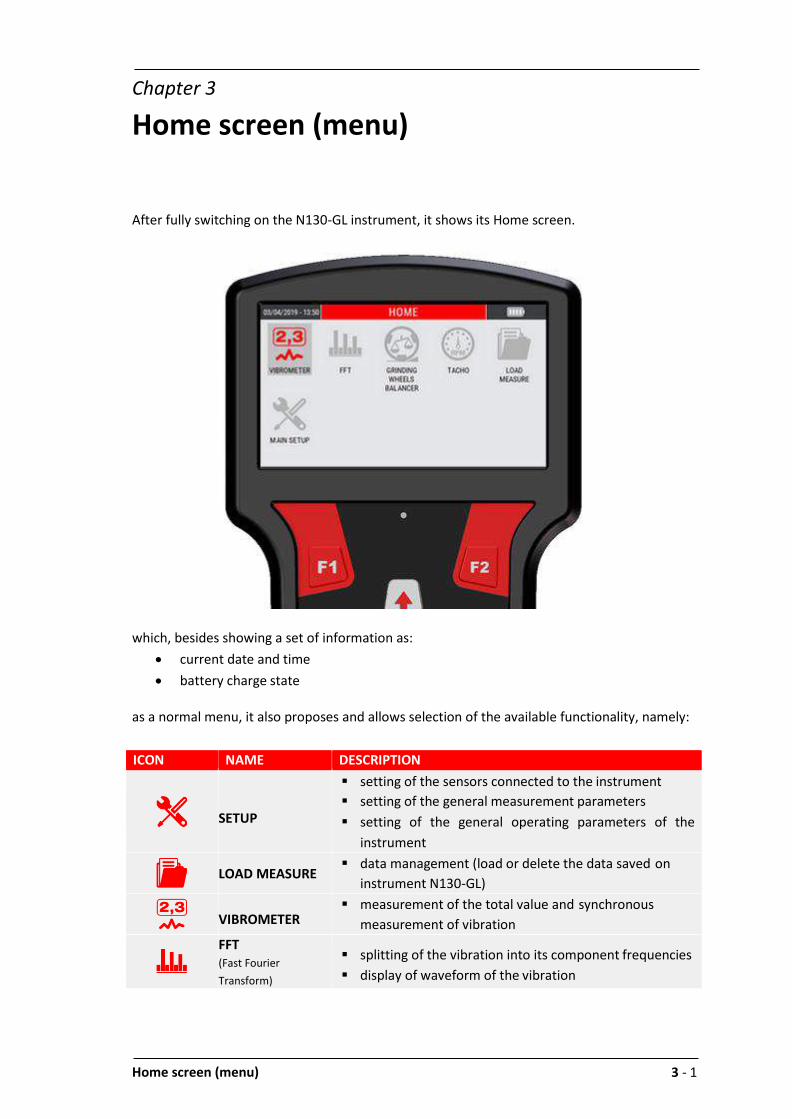
Grinding wheel balancer mode 7 - 9
Stop the measurement with a further pressure of .
Attention:
The average speed value is very important because the calibration procedure
can be considered to be well executed only if between each step this speed
does not show differences greater than 5%. The control of this condition is
left to the operator.
Correction run: spin with sliding weights in balancing position
After to be done the launch with weight "B" moved to known position (see 7.7 – Test
run: spin with a known weight in known position), press (NEXT) to go to the final
step.
The instrument indicates the right positions where the sliding weights must be
positioned to balance the grinding wheel.
Move the sliding weights as required, press to continue.
The key (HOME) allows to back to the instrument home page.

7 - 10 Grinding wheel balancer mode
Note:
Use the key (NEXT) to go to the next vibration acquisition screen.
In case key is pressed incorrectly, a warning indicates the exact procedure
to follow.
Note:
From this point, going back to the instrument home page and accessing again
to the function, will be available the item "Use current project" (see 7.4 - Use
current project).
Press (NEXT) to go to the measurement screen.
Press to start the measurement; as for the previous step, is displayed the bar that
shows the quality of the measurement in real time.

Grinding wheel balancer mode 7 - 11
Stop the measurement with a further pressure of .
If the vibration value reached is good, press (END) to complete/end the balancing
procedure (FINAL REPORT).
On the other hand, if the vibration value is NOT good, press (REFINE) to refine the
position of the sliding weights.
Move the sliding weights as required; press (NEXT) to go to the measurement
screen.
Press to start the measurement; as for the previous step, is displayed the bar that
shows the quality of the measurement in real time.

7 - 12 Grinding wheel balancer mode
Stop the measurement with a further pressure of .
Key (END) goes to the "FINAL REPORT" page, reporting the values of vibration and
unbalance preceding and following the balancing procedure.
1. Project name (shown only when the project is saved) 2. Initial synchronous vibration (before balancing procedure) 3. Final synchronous vibration (after balancing procedure) 4. Initial sliding weight position (before balancing procedure) 5. Final sliding weight position (after balancing procedure)
1
2
3
4
5
Grinding wheel balancer mode 7 - 13
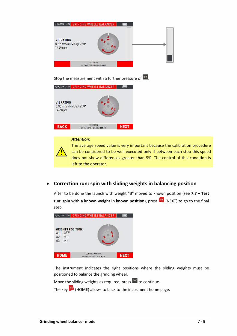
MENU function
Access to the menu using the key . The following functionalities are available here:
Save project
From the menu select the "Save project" item by pressing the key .
Type the desired name for the project; each single letter composing the name must be
selected by moving with the "arrow" keys on the alphanumeric keypad visible on the
display, and confirming the selection by pressing .
Press key (DONE) to confirm the project name.
Note:
For each single letter, use the "arrow" keys and to confirm the choices.
Note:
For the format type of the saved data and its management, refer to appendix
E - "The JSON file"

7 - 14 Grinding wheel balancer mode
Take Screenshot
Allows to "capture" the image on the display by saving it as a .png file (see "Take
screenshot" function 2-7).
Press to continue.

“TACHO” mode 8 - 1
Chapter 8
“TACHO” mode
Before proceeding with more in-depth analysis, operators may sometimes need to detect the
rotation velocity of one or more of the shafts with a high degree of precision.
The N130-GL instrument has a precise tachometer function, capable of measuring rotation
speed of up to 250.000 RPM.
“TACHO” – measurement screen
he measurement page supplies a series of information, organized as shown in the figure:
1. detected speed value (expressed in RPM)
Note:
Before to use the TACHO mode, apply a suitable reflecting sticker on the rotating body
as a point of reference (0°).
Connect the photocell (optional) to the N130 instrument and position it at a distance
of between 60 and 1000 mm from the rotating body.
For the photocell setup see “Appendix D – Photocell for instruments CEMB Nx30”.
Caution:
Take great care when positioning the photocell: as the rotating body requires manual
intervention, make sure that it is still and cannot be started up accidentally.
If the rotating body cannot be rotated by hand when positioning the photocell, it
should be positioned in points in which the LEDs are visible without having to get too
close to the moving bodies.
1

8 - 2 “TACHO” mode
Measurement of a “TACHO” value
Select the TACHO mode from the main page of the instrument by pressing the key .
At the first access to the function after switching on the instrument, if no measurement has
been performed yet, an alarm reminds to connect the sensors before making the
measurement.
Press to start the measurement; the instrument acquires continuously, press again to
freeze the acquisition.
MENU function
Access to the menu using the key . The following functionalities are available here:
Take Screenshot
Allows to "capture" the image on the screen by saving it as a .png file (see Function
"Take screenshot" 2-7).
Technical data A - 1
Appendix A
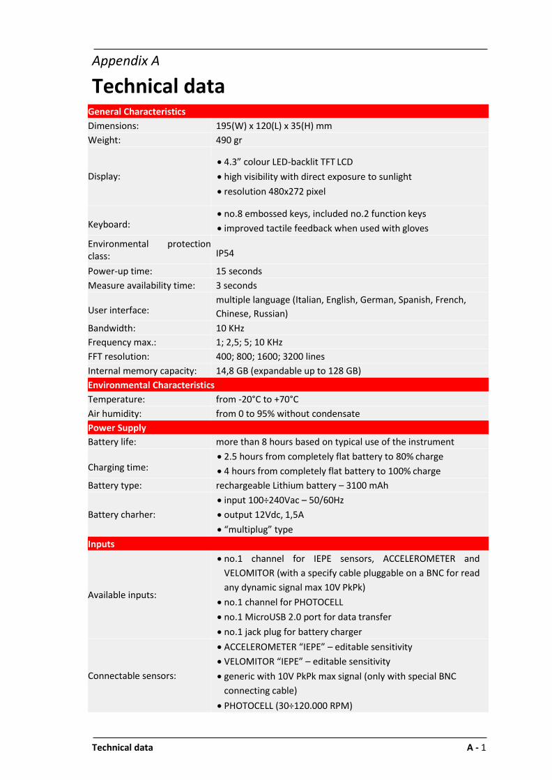
Technical data
General Characteristics
Dimensions: 195(W) x 120(L) x 35(H) mm
Weight: 490 gr
Display:
4.3” colour LED-backlit TFT LCD
high visibility with direct exposure to sunlight
resolution 480x272 pixel
Keyboard: no.8 embossed keys, included no.2 function keys
improved tactile feedback when used with gloves
Environmental protection class: IP54
Power-up time: 15 seconds
Measure availability time: 3 seconds
User interface: multiple language (Italian, English, German, Spanish, French,
Chinese, Russian)
Bandwidth: 10 KHz
Frequency max.: 1; 2,5; 5; 10 KHz
FFT resolution: 400; 800; 1600; 3200 lines
Internal memory capacity: 14,8 GB (expandable up to 128 GB)
Environmental Characteristics
Temperature: from -20°C to +70°C
Air humidity: from 0 to 95% without condensate
Power Supply
Battery life: more than 8 hours based on typical use of the instrument
Charging time: 2.5 hours from completely flat battery to 80% charge
4 hours from completely flat battery to 100% charge
Battery type: rechargeable Lithium battery – 3100 mAh
Battery charher:
input 100÷240Vac – 50/60Hz
output 12Vdc, 1,5A
“multiplug” type
Inputs
Available inputs:
no.1 channel for IEPE sensors, ACCELEROMETER and
VELOMITOR (with a specify cable pluggable on a BNC for read
any dynamic signal max 10V PkPk)
no.1 channel for PHOTOCELL
no.1 MicroUSB 2.0 port for data transfer
no.1 jack plug for battery charger
Connectable sensors:
ACCELEROMETER “IEPE” – editable sensitivity
VELOMITOR “IEPE” – editable sensitivity
generic with 10V PkPk max signal (only with special BNC
connecting cable)
PHOTOCELL (30÷120.000 RPM)

A - 2 Technical data
Carrying case
Dimensions: approx. 440(W) x 360(L) x 145(H) mm
Weight complete of
Standard accessories: approx. 3100 gr
Measurement types
Measure mode: effective value [RMS]
Peak value [Pk]
Peak-to-Peak value [PkPk]
Measure units: acceleration - [g]
velocitity - [mm/s] or [inch/s]
displacement - [µm] or [mils]
frequency - [Hz] or [CPM]
rotation speed - [RPM]
Note:
This device uses the Qt Toolkit 4.8.4 under the terms of the GNU Lesser General
Public License (LGPL) v. 2.1.
The full text of the GPL and LGPL licenses can be found on the USB stick supplied with
this device and on https://www.gnu.org/licenses.
In compliance with LGPL, this device dynamically links to the unmodified Qt libraries,
as provided by the Qt Company.
The Qt Toolkit is copyright by The Qt Company Ltd. (www.qt.io) and/or its subsidiary(-
ies) and other contributors.
Qt and the Qt logo are trademarks of The Qt Company Ltd.
This device is based in part on the work of the Qwt project
(https://qwt.sourceforge.io/).

Evaluation criteria B - 1
Appendix B
Evaluation criteria
ISO 10816-3 Mechanical vibration - Evaluation of machine vibration by measurements on non-
rotating parts - Part 3: industrial machines with nominal power above 15 kW and nominal
speeds between 120 r/min and 15 000 r/min when measured in situ.
Introduction
ISO 10816-3 constitutes the basic document that describes the general requirements for
evaluation of vibration in different types of machinery when the vibration measurements are
made on non-rotating parts. It provides specific guidance to assess the severity of the vibration
measured on bearings, bearing supports or industrial machine casings when the
measurements are made in situ.
Measurement points
Normally, the measurements should be made on the visible parts of the machine which are
usually accessible. Due care should be taken so that the measurements are reasonably
representative of vibration of the bearing seat and do not lead to any local resonance or
amplification. The vibration measurement positions and directions must be such as to offer
adequate sensitivity to the dynamic forces of the machine. Generally, this requires two
orthogonal radial measurement positions on each bearing cap or support as illustrated in
Figures 1 and 2.
The sensors can be arranged in any angular position on the bearing housings or supports. For
horizontally mounted machines, it is generally preferable to arrange the sensors in vertical and
horizontal position. For inclined or vertically mounted machines, the position that gives the
maximum vibration reading, normally in the direction of the flexible shaft, must be one of
those used. In some cases, measurement in axial direction is also advisable.
On a bearing cap or support, only one sensor can be used instead of the more usual pair of
orthogonal sensors if it is known that this sensor provides sufficient information on the
machine vibration amplitude. However, precautions must be taken when evaluating vibration
using only one sensor at the level of a measurement plane, as you risk it not being oriented to
provide a reasonable approximation of the maximum value on this plane.

B - 2 Evaluation criteria
Classification according to machine type, nominal power or shaft height
Significant differences in design, type of bearings and type of support structures require a
division into different machine groups (as regards the shaft height, see ISO 496). The machines
in the 4 groups below may have a horizontal, vertical or inclined shaft and may be mounted on
rigid or flexible supports.
Group 1: Large machines with nominal power above 300 kW or electrical machines with shaft
heights H ≥ 315 mm.
These machines normally have sleeve bearings. The range of operating or nominal
speeds is relatively broad with ranges from 120 r/min to 15 000 r/min.
Group 2: Medium-sized machines with nominal power above 15 kW up to and including 300
kW or electrical machines with shaft heights from 160 mm up to ≥ 315 mm.
These machines normally have rolling bearings and an operating speed above 600
rpm
Group 3: Pumps with fin rotors and separate motor (mixed or axial flow centrifugal pumps)
with nominal power above 15 kW.
The machines in this group may have sleeve or rolling bearings.
Figure 1 Measurement points Figure 2 Measurement points for vertical machine units

Evaluation criteria B - 3
Group 4: Pumps with fin rotors and incorporated motor (mixed or axial flow centrifugal
pumps) with nominal power above 15 kW.
The machines in this group normally have sleeve or rolling bearings.
Classification according to support f lexibi l ity
The flexibility of the support unit in the specified directions is classified considering two
possibilities:
– rigid supports
– flexible supports
These support conditions are determined by the ratio between the flexibility of the machine
and that of its foundation. If the natural lowest frequency of the combined machine-support
system in the measuring direction is greater by at least 25% than the main excitation
frequency (in most cases, this is the rotation frequency) in this direction, the support system
may be considered rigid. All other support systems may be considered flexible.
Typical examples: large and medium-sized electrical motors, mainly with low speeds, have rigid
supports, while turbo generators and compressors with power above 10 MW and vertical
machine units normally have flexible supports.
In certain cases, a support may be rigid in one direction and flexible in the other. For example,
the natural lowest frequency in vertical direction may be well above the main excitation
frequency, while the natural frequency in horizontal direction may be considerably lower. Such
a system would be rigid on the vertical but flexible on the horizontal plane. In these cases, the
vibration should be evaluated according to the classification of the support that corresponds
to the measuring direction.
If the machine-support system class cannot easily be determined from drawings or calculated,
it can be determined with tests.
Evaluation zones
The following evaluation zones are defined to allow qualitative vibration evaluation of a given
machine and to provide guidelines for any action to be taken.
Zone A: the vibration of newly commissioned machines normally falls within this zone;
Zone B: machines with vibration within this zone are normally considered acceptable for
unrestricted long-term operation;

B - 4 Evaluation criteria
Zone C: machines with vibration within this zone are normally considered unsatisfactory for
long-term continuous operation. Generally, the machine may be operated for a limited
period in this condition until a suitable opportunity arises for remedial action;
Zone D: vibration values within this zone are normally considered to be of sufficient severity to
cause damage to the machine.
The numerical values specified are not intended to serve as the only basis for acceptance
specifications, but should be agreed upon between the machine manufacturer and the
customer. Nevertheless, the vibration limits for the zone boundaries provide guidelines for
ensuring that gross deficiencies or unrealistic requirements are avoided. In certain cases,
particular construction solutions may be adopted for a given machine, which would require
adopting different values (greater or smaller) for the zone limits. In these cases, the machine
manufacturer generally needs to explain the reasons and, in particular, confirm that the
machine would not be damaged by operation at higher vibration values.
Evaluation zone limits
Table A.1 Classification of the vibration severity zones for Group 1 machines: Large
machines with nominal power above 300 kW but not greater than 50 MW
or electrical machines with shaft heights H ≥ 315 mm
Support class Zone limit Effective velocity mm/s
Rigid
A/B 2,3
B/C 4,5
C/D 7,1
Flexible
A/B 3,5
B/C 7,1
C/D 11,0

Evaluation criteria B - 5
Table A.2 Classification of the vibration severity zones for Group 2 machines:
Medium-sized machines with nominal power above 15kW up to and
including 300 kW or electrical machines with shaft heights from 160 mm
up to ≤ 315 mm
Support class Zone limit Effective velocity mm/s
Rigid
A/B 1,4
B/C 2,8
C/D 4,5
Flexible
A/B 2,3
B/C 4,5
C/D 7,1
Table A.3 Classification of the vibration severity zones for Group 3 machines:
Pumps with fin rotors and separate motor (mixed or axial flow
centrifugal pumps) with nominal power above 15 kW
Support class Zone limit Effective velocity mm/s
Rigid
A/B 2,3
B/C 4,5
C/D 7,1
Flexible
A/B 3,5
B/C 7,1
C/D 11,0
Table A.4 Classification of the vibration severity zones for Group 4 machines: Pumps with
fin rotors and incorporated motor (mixed or axial flow centrifugal pumps) with
nominal power above 15 kW
Support class Zone limit Effective velocity mm/s
Rigid
A/B 1,4
B/C 2,8
C/D 4,5
Flexible
A/B 2,3
B/C 4,5
C/D 7,1

B - 6 Evaluation criteria
Empty page

A rapid guide to interpreting a spectrum C - 1
Appendix C
A rapid guide to interpreting a spectrum
TYPICAL CASES OF MACHINE VIBRATIONS
1. PRELIMINARY RAPID GUIDE
Measured values during control
f = vibration frequency [cycles/min] or [Hz]
s = shift amplitude [µm]
v = vibration speed [mm/s]
a = vibration acceleration [g]
n = piece rotation speed [rpm]
Frequency data Causes Notes
1) f = n Unbalances in rotating bodies.
Rotor inflection.
Resonance in rotating bodies.
Intensity proportional to unbalance, mainly in the radial
direction, increases with speed.
Axial vibrations sometimes sensitive.
Critical speed near n with very high intensity.
Roller bearings mounted with
eccentricity.
Misalignments.
Recommend balancing the rotor on its own bearings.
Considerable axial vibration also present, greater than 50% of
the transverse vibration; also frequent cases of f = 2n, 3n.
Eccentricity in pulleys, gears, etc…
When the rotation axis does not coincide with the geometric
axis.
Irregular magnetic field in electrical
machines.
Vibration disappears when power is cut off.
Belt length an exact multiple of the
pulley circumference.
Stroboscope can be used to block belts and pulleys at the same
time.
Gear with defective tooth.
An unbalance vibration often also intervenes.
Alternating forces. Second and third harmonic present.
2) f n with knocking Mechanical unbalance defect
superimposed on irregular magnetic
field.
In asynchronous motors, the knocking is due to running.
3) f (0,40 ÷ 0,45) n Defective lubrication in sleeve
bearings.
For high n, above the 1° critical level.
Check with stroboscope.
Precision journal movement (oil whirl).
Faulty roller bearing cage. Check for harmonics.
4) f = ½ n Mechanical weakness in rotor.
Sleeve bearing shells loose.
Mechanical yield.
This is a sub-harmonic, often present but hardly ever important.
f = 2n, 3n, 4n and semi-harmonics also often present.

C - 2 A rapid guide to interpreting a spectrum
Frequency data Causes Notes
5) f = 2n Misalignment.
Mechanical looseness.
There is strong axial vibration.
Loose bolts, excessive play in the mobile parts and bearings, cracks and
breaks in the structure: there are upper grade sub-harmonics.
6) f is an exact
multiple of n
Roller bearings misaligned or forced
in their housings.
Defective gears.
Frequency = n x number of spheres or rollers. Check with stroboscope.
f = z n (z = number of defective teeth).
Because of general wear, teeth badly made if z = total number of teeth.
Misalignments with excessive axial
play.
Often caused by mechanical looseness.
Rotors with blades (pumps, fans). f = n x number of blades (or channels)
7) f is much greater
than n, not an exact
multiple
Damaged roller bearings. Unstable frequency, intensity and phase.
Axial vibration.
Excessive wear on sleeve bearings. Completely or locally defective lubrication.
Audible screech.
Belts too tight. Characteristic audible screech.
Multiple belts not homogeneous. Run between the belts.
Low load gears. Teeth knock together because of insufficient load; unstable vibration.
Rotors with blades for fluid
management (cavitation, reflux,
etc.).
Unstable frequency and intensity.
f = n x number of blades x number of channels.
Frequent axial vibration.
8) f = natural
frequency of other
parts
Excessive play on sleeve bearings. Oil whip caused by vibrations in other parts.
Check with stroboscope.
Belts disturbed by vibrations from
other parts.
Examples: eccentric or unbalanced pulleys, misalignments, rotor
unbalances.
9) f unstable with
knocking
Multiple belts not homogeneous.
Belts with multiple joints.
Unstable intensity.
10) f = nc
n nc
(nc = critical speed of shaft)
Roller bearings.
For rotors above the 1st critical speed.
(nr = mains frequency)
Electric motors, generators
Harmonics also present.
12) f = fc < n or f = 2 fc Belt with defective elasticity in one
area.
fc is the belt frequency.
fc = D n / l (D = pulley diameter; l = belt length).
Considerable axial vibrations, more than 10% of the transverse vibration, may be caused typically by:
shaft inflection, especially in electrical motors;
defective thrust bearings;
elliptic eccentricity in the electric motor rotor;
forces deriving from tubing;
distorted foundations;
wear in stuffing box seals, etc.;
rotor side rubbing;
defective radial bearings;
defective coupling;
defective belts.

A rapid guide to interpreting a spectrum C - 3
2. TYPICAL SPECTRA OF VIBRATIONS RELATED TO THE MOST COMMON DEFECTS
Note:
The spectra are in an indicative graphic form. The N130 equipment produces a
different form of graph.
The following are the spectra of typical vibrations, caused by the most common defects found
in practical experience.
Note:
CPM = shaft rotation speed in RPM.
1. UNBALANCE
2. MISALIGNMENT

C - 4 A rapid guide to interpreting a spectrum
3. MECHANICAL LOOSENESS
4. BELT
5. GEARS
SIDE BANDS
GEAR MESH FREQUENCY
2x BELT FREQUENCY

A rapid guide to interpreting a spectrum C - 5
6. SLEEVE BEARINGS
7. ROLLER BEARINGS
8. ELECTRIC MOTORS
2x LINE FREQUENCY
TYPICAL FREQUENCIES OF
BEARING DEFECTS

C - 6 A rapid guide to interpreting a spectrum
3. FORMULAE FOR CALCULATING TYPICAL BEARING DEFECT FREQUENCIES
The most common case:
a - fixed external ring (rotating internal ring)
cos
PD
BDS=FTF 1
2 Housing frequency
cos
PD
BDN
S=BPFO 1
2 Defect on outer track
cos
PD
BD+N
S=BPFI 1
2 Defect on inner track
2
12
cosPD
BD
BD
PDS=BSP Defect on roller/ball
b - rotating external ring (fixed internal ring)
cos
PD
BDS=FTF 1
2 Housing frequency
cos
PD
BDN
S=BPFO 1
2 Defect on outer track
cos
PD
BD+N
S=BPFI 1
2 Defect on inner track
2
12
cosPD
BD
BD
PDS=BSP Defect on roller/ball
The frequencies of bearings can be calculated if we know:
S = number of shaft rpm
PD = primitive diameter BD = ball/roller diameter
N = number of balls/rollers
Θ = angle of contact
Approximate calculation formulae (± 20%)
FTF = 0.4 x S (a) or 0.6 x S (b)
BPFO = 0.4 x N x S (a) or (b)
BPFI = 0.6 x N x S (a) or (b)
BSP = 0.23 x N x S (N < 10) (a) or (b)
= 0.18 x N x S (N ≥10) (a) or (b)

Photocell for instruments CEMB Nx30 D - 1
Appendix D
Photocell for instruments CEMB Nx30
Specifications:
CEMB complete code: 920X30025
Distance from target: 60 ÷ 1000 mm
Current consuption: 30mA nominal
Spare parts:
CEMB sensor only, code: 800625310
CEMB cable 2 meters only, code: 962020718
Connections:
CONNETTOR PINOUT
(Yellow connector)
1 - +24 VDC
5 – TACHO IN
8 - GROUND + SHIELDING
Reflector position on rotor or shaft:
1. Stick a piece of reflective tape on the rotor;
2. It must be at least twice the size of the laser spot;
3. The laser beam should hit the spotlight center.

D - 2 Photocell for instruments CEMB Nx30
Photocell calibration:
STEP DESCRIPTION
1
With photocell power-on (green LED on), touch the
back of the photocell with a tool (e.g. screwdriver)
for 2 seconds
2
LEDs green and yellow flashing (frequency 1 Hz)
3
Align photocell spot to the target(reflective tape
sticked on the shaft/impeller)
4
Touch quickly the back of the photocell with a tool,
to confirm target acquisition
5
Calibration successful
6
Calibration failed
Note:
It is also possible not use a reflector. If there is a difference in color between the
marker used and the shaft/impeller, can be used other types of markers (colored
adhesive tape, matte paint marker, etc.).
Caution: If there is more than one target the speed detected will not be the correct one.

The JSON format E - 1
Appendix E
The JSON format
The N130 uses JSON files to store the different measures.
JSON (JavaScript Object Notation) is an open standard format for data exchange. For people it
is easy to read and write, while for machines it is easy to generate and analyze.
JSON is a text format completely independent of the programming language.
Libraries and functions for parsing and JSON data generation are available in all popular
languages. This feature makes JSON an ideal language for data exchange.
JSON is a self-documenting format that describes both the structure and names of the fields,
as well as their value. It has a rigid syntax that allows an implementation of simple, efficient
and consistent parsing algorithms.
JSON is based on two structures:
A set of name/value pairs
An ordered list of values
These are universal data structures. Virtually all modern programming languages support them
in both forms.
In JSON, they take these forms:
An object is an unordered series of names/values. An object begins with { (left brace) and ends
with } (right brace). Each name is followed by : (colon) and the name/value pair is separated by
, (comma).
An array is an ordered collection of values. An array begins with [ (left bracket) and ends with ]
(right bracket). Values are separated by , (comma).

E - 2 The JSON format
A value can be a string in quotes, or a number, either true or false, or an object or an array.
These structures can be nested.
Using these basic structures, JSON can represent the most complex data structures: records,
lists, trees ...
The use of a standard and open format like JSON makes it extremely easy to create macros or
applications to extract the necessary information and use them according to your needs.
MS Excel allows to import JSON files directly from the version “2016”. For previous versions
can be used Power Queries or VBA macros.
Detailed information on the JSON format are available online.
As an example:
https://json.org/
ECMA-404 The JSON Data Interchange Standard
[http://www.ecma-international.org/publications/files/ECMA-ST/ECMA-404.pdf]
JSON file online reader
http://jsonviewer.stack.hu/
N130-GL measurement archive
The N130-GL device organizes the measurement archive in projects.
Each project is saved in a different JSON file, whose name is the name chosen for the project.
All projects are available on the device, within the folder <N130\archive>.
Each file is organized with a tree structure:
Measurement point (Support number / direction) - for example "point 3x"
o Array of measures
Measurement

The JSON format E - 3
All measurements have common information:
An object called "measureType" whose value is a string corresponding to the measure
type
o OVERALL measurement saved in the Vibrometer function
o SYNC 1x measurement saved in the Vibrometer 1xRPM function
o FFT measurement saved in the FFT function
o SMART ANALYSIS measurement saved in the Smart Analysis function
o CBA measurement saved in the CBA bearing analysis
function
An object called "dateTime" whose value is a string with the measurement acquisition
date and time (in ISO 8601 format)
When necessary, each measurement also contains the settings with which it was acquired.
The various measures are saved with the following structure.
OVERALL
{
"main peak":{
"amplitude":{
"value":9.7,
"unit":"mm/s",
"unit mode":"RMS"
},
"frequency":{
"value":46.5,
"unit":"Hz"
}
},
"overall":{
"value":3.6,
"unit":"mm/s",
"unit mode":"RMS"
},
"dateTime":"2018-12-17T12:23:42",
"setup":{
"max frequency":{
"value":1000.0,
"unit":"Hz"
},
"high-pass frequency":{
"value":0.0,
"unit":"Hz"
},
"No. of lines":400,
"No. of averages":2
},
"measureType":"OVERALL"
}
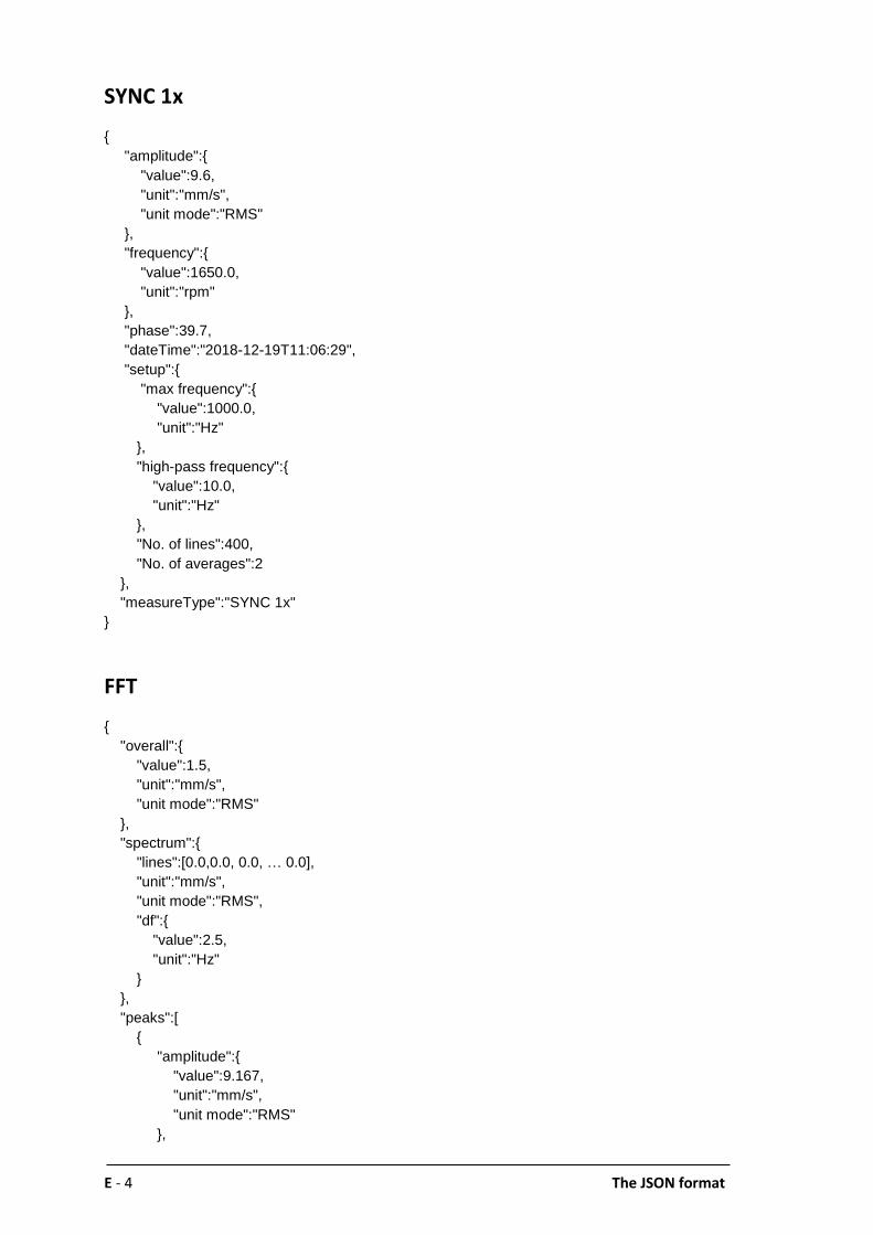
E - 4 The JSON format
SYNC 1x
{
"amplitude":{
"value":9.6,
"unit":"mm/s",
"unit mode":"RMS"
},
"frequency":{
"value":1650.0,
"unit":"rpm"
},
"phase":39.7,
"dateTime":"2018-12-19T11:06:29",
"setup":{
"max frequency":{
"value":1000.0,
"unit":"Hz"
},
"high-pass frequency":{
"value":10.0,
"unit":"Hz"
},
"No. of lines":400,
"No. of averages":2
},
"measureType":"SYNC 1x"
}
FFT
{
"overall":{
"value":1.5,
"unit":"mm/s",
"unit mode":"RMS"
},
"spectrum":{
"lines":[0.0,0.0, 0.0, … 0.0],
"unit":"mm/s",
"unit mode":"RMS",
"df":{
"value":2.5,
"unit":"Hz"
}
},
"peaks":[
{
"amplitude":{
"value":9.167,
"unit":"mm/s",
"unit mode":"RMS"
},

The JSON format E - 5
"frequency":{
"value":45.3125,
"unit":"Hz"
}
},
…
{
"amplitude":{
"value":0.78,
"unit":"mm/s",
"unit mode":"RMS"
},
"frequency":{
"value":252.5,
"unit":"Hz"
}
}
],
"dateTime":"2018-12-20T09:40:27",
"setup":{
"max frequency":{
"value":1000.0,
"unit":"Hz"
},
"high-pass frequency":{
"value":10.0,
"unit":"Hz"
},
"No. of lines":400,
"No. of averages":2
},
"measureType":"FFT"
}
The wheel balancing archive The N130-GL instrument organizes the archive of wheel balances in projects.
All projects are saved in a single JSON file, available in the device
<N130-GL\archive\balancing\grinding_wheels\GrindingBalancing.json>.
The file is organized with a tree structure:
• Array of projects
o Project

E - 6 The JSON format
The various projects are saved with the following structure.
GrindingBalancing Project { "name":"project name", "data":{ "clockwise":true, "calibration":{ "calibration runs":[ { "done":true, "Sync 1x vibration":{ "amplitude":{ "value":2.5, "unit":"mm/s", "unit mode":"RMS" }, "phase":199.0 }, "speed":{ "value":1890.0, "unit":"rpm" } "trial weights":[0.0,180.0], }, { "done":true, "Sync 1x vibration":{ "amplitude":{ "value":4.8, "unit":"mm/s", "unit mode":"RMS" }, "phase":48.0 }, "speed":{ "value":1900.0, "unit":"rpm" } "trial weights":[0.0,90.0], } ] }, "balancing": { "Sync 1x vibrations":[ { "amplitude":{ "value":2.5, "unit":"mm/s", "unit mode":"RMS" }, "phase":199.0 }, { "amplitude":{ "value":3.9, "unit":"mm/s", "unit mode":"RMS" }, "phase":25.1 } ],

The JSON format E - 7
"speeds":[ { "value":1890.0, "unit":"rpm" }, { "value":1895.0, "unit":"rpm" } ], "correction weights":[[31.75,355.21]] }, }, "dateTime":"2019-03-14T10:00:00" }

E - 8 The JSON format
Empty page