Vertically aligned accelerometer for wheeled vehicle odometry
9
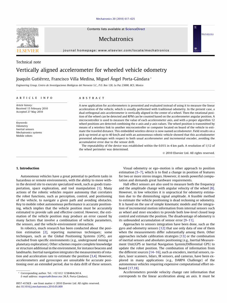
Technical note Vertically aligned accelerometer for wheeled vehicle odometry Joaquín Gutiérrez, Francisco Villa Medina, Miguel Ángel Porta-Gándara * Engineering Group, Centro de Investigaciones Biológicas del Noroeste S.C., P.O. Box 128, La Paz 23000, BCS, Mexico article info Article history: Received 15 February 2010 Accepted 27 May 2010 Keywords: Odometry Inertial sensors Mechatronics systems Mobile robots abstract A new application for accelerometers is presented and evaluated instead of using it to measure the linear acceleration of the vehicle, which is usually performed with traditional odometry. In the present case, a dual orthogonal axis accelerometer is vertically aligned in the center of a wheel. Then the rotational posi- tion of the wheel can be detected and RPM can be counted based on the accelerometer angular position. A microcontroller is used to measure the value of each accelerometer axis, and with a proper algorithm 12 wheel positions are detected combining the x-axis and y-axis values. The wheel position is transmitted by means of a wireless link to another microcontroller or computer located on board of the vehicle to esti- mate the traveled distance. This embedded wireless device is now named accelodometer. Field results on a pick-up tested at up to 40 km/h and with an autonomous robotic vehicle showed that this accelodometer presented advantages with respect to both usual accelerometer and incremental encoder, avoiding the accumulative error due to the sensor drift. The repeatability of the device was established within the 0.01% in 4 km path. A resolution of 1/12 of the wheel perimeter was determined. Ó 2010 Elsevier Ltd. All rights reserved. 1. Introduction Autonomous vehicles have a great potential to perform tasks in hazardous or remote environments, with the ability to move with- in the desired site to execute specialized work, such as goods trans- portation, space exploration, and tool manipulation [1]. Many actions of the robotic vehicles require autonomy that correlates the robot functions, such as perception, control, and positioning of the vehicle, to navigate a given path and avoiding obstacles. Key to mobile robot autonomous performance is accurate position- ing, which implies that the vehicle position must be accurately estimated to provide safe and effective control. However, the esti- mation of the vehicle position may produce an error caused by many factors that involve a combination of vehicle parameters, the sensors, and the vehicle-environment interaction. In robotics, much research has been conducted about the posi- tion estimation [2], reporting numerous techniques; some techniques, such as the Global Positioning Systems (GPS), are excluded from specific environments (e.g., underground mining or planetary exploration). Other schemes require complete knowledge or structure additional in the environment, for instance beacons and landmarks. Inertial navigation integrates the measurements of rota- tion and acceleration rate to estimate the position [3,4]. However, accelerometers and gyroscopes are unsuitable for accurate posi- tioning over an extended period, due to data drift of these sensors. Visual odometry or ego–motion is other approach to position estimation [5–7], which is to find a change in position of features for two or more stereo images. However, it needs powerful compu- tation and demands great hardware requirements. Hall effect sensors are also used to measure both the frequency and the amplitude change with angular velocity of the wheel [8]. However, in low velocities it is unpractical for odometry estima- tion due to the diminishing signal amplitude. A feasible method to estimate the vehicle positioning is dead reckoning or odometry. It is based on the use of simple kinematic models and the integra- tion of incremental motion information from internal sensors such as wheel and steer encoders to provide both low-level closed loop control and estimate the position. The disadvantage of odometry is its unbounded accumulation of sensor error [9–11]. Approaches to sensors integration have been done, such as the gyro and odometry sensors [12] that use only data of one of them when the measurements differ substantially among them. Other approaches include calibration strategies [13] or the combination of inertial sensors and absolutes positioning (e.g., Inertial Measure- ment Unit/GPS or Inertial Navigation System/Differential GPS) to update the robot position. The combination of information from the different sources [14–16], such as encoders, inertial sensors, ra- dars, laser scanners, lidars, IR sensors, and cameras, have been ex- plored in many applications (e.g., DARPA Challenge) of the autonomous vehicles requiring expensive computational effort on- board [17,18]. Accelerometers provide velocity change rate information that corresponds to the linear acceleration along an axis. It must be 0957-4158/$ - see front matter Ó 2010 Elsevier Ltd. All rights reserved. doi:10.1016/j.mechatronics.2010.05.009 * Corresponding author. Tel.: +52 612 1238484x3614. E-mail address: [email protected] (M.Á. Porta-Gándara). Mechatronics 20 (2010) 617–625 Contents lists available at ScienceDirect Mechatronics journal homepage: www.elsevier.com/locate/mechatronics
-
Upload
independent -
Category
Documents
-
view
1 -
download
0
Transcript of Vertically aligned accelerometer for wheeled vehicle odometry
Mechatronics 20 (2010) 617–625
Contents lists available at ScienceDirect
Mechatronics
journal homepage: www.elsevier .com/ locate/mechatronics
Technical note
Vertically aligned accelerometer for wheeled vehicle odometry
Joaquín Gutiérrez, Francisco Villa Medina, Miguel Ángel Porta-Gándara *
Engineering Group, Centro de Investigaciones Biológicas del Noroeste S.C., P.O. Box 128, La Paz 23000, BCS, Mexico
a r t i c l e i n f o a b s t r a c t
Article history:Received 15 February 2010Accepted 27 May 2010
Keywords:OdometryInertial sensorsMechatronics systemsMobile robots
0957-4158/$ - see front matter � 2010 Elsevier Ltd. Adoi:10.1016/j.mechatronics.2010.05.009
* Corresponding author. Tel.: +52 612 1238484x36E-mail address: [email protected] (M.Á. Porta-G
A new application for accelerometers is presented and evaluated instead of using it to measure the linearacceleration of the vehicle, which is usually performed with traditional odometry. In the present case, adual orthogonal axis accelerometer is vertically aligned in the center of a wheel. Then the rotational posi-tion of the wheel can be detected and RPM can be counted based on the accelerometer angular position. Amicrocontroller is used to measure the value of each accelerometer axis, and with a proper algorithm 12wheel positions are detected combining the x-axis and y-axis values. The wheel position is transmitted bymeans of a wireless link to another microcontroller or computer located on board of the vehicle to esti-mate the traveled distance. This embedded wireless device is now named accelodometer. Field results on apick-up tested at up to 40 km/h and with an autonomous robotic vehicle showed that this accelodometerpresented advantages with respect to both usual accelerometer and incremental encoder, avoiding theaccumulative error due to the sensor drift.
The repeatability of the device was established within the 0.01% in 4 km path. A resolution of 1/12 ofthe wheel perimeter was determined.
� 2010 Elsevier Ltd. All rights reserved.
1. Introduction
Autonomous vehicles have a great potential to perform tasks inhazardous or remote environments, with the ability to move with-in the desired site to execute specialized work, such as goods trans-portation, space exploration, and tool manipulation [1]. Manyactions of the robotic vehicles require autonomy that correlatesthe robot functions, such as perception, control, and positioningof the vehicle, to navigate a given path and avoiding obstacles.Key to mobile robot autonomous performance is accurate position-ing, which implies that the vehicle position must be accuratelyestimated to provide safe and effective control. However, the esti-mation of the vehicle position may produce an error caused bymany factors that involve a combination of vehicle parameters,the sensors, and the vehicle-environment interaction.
In robotics, much research has been conducted about the posi-tion estimation [2], reporting numerous techniques; sometechniques, such as the Global Positioning Systems (GPS), areexcluded from specific environments (e.g., underground mining orplanetary exploration). Other schemes require complete knowledgeor structure additional in the environment, for instance beacons andlandmarks. Inertial navigation integrates the measurements of rota-tion and acceleration rate to estimate the position [3,4]. However,accelerometers and gyroscopes are unsuitable for accurate posi-tioning over an extended period, due to data drift of these sensors.
ll rights reserved.
14.ándara).
Visual odometry or ego–motion is other approach to positionestimation [5–7], which is to find a change in position of featuresfor two or more stereo images. However, it needs powerful compu-tation and demands great hardware requirements.
Hall effect sensors are also used to measure both the frequencyand the amplitude change with angular velocity of the wheel [8].However, in low velocities it is unpractical for odometry estima-tion due to the diminishing signal amplitude. A feasible methodto estimate the vehicle positioning is dead reckoning or odometry.It is based on the use of simple kinematic models and the integra-tion of incremental motion information from internal sensors suchas wheel and steer encoders to provide both low-level closed loopcontrol and estimate the position. The disadvantage of odometry isits unbounded accumulation of sensor error [9–11].
Approaches to sensors integration have been done, such as thegyro and odometry sensors [12] that use only data of one of themwhen the measurements differ substantially among them. Otherapproaches include calibration strategies [13] or the combinationof inertial sensors and absolutes positioning (e.g., Inertial Measure-ment Unit/GPS or Inertial Navigation System/Differential GPS) toupdate the robot position. The combination of information fromthe different sources [14–16], such as encoders, inertial sensors, ra-dars, laser scanners, lidars, IR sensors, and cameras, have been ex-plored in many applications (e.g., DARPA Challenge) of theautonomous vehicles requiring expensive computational effort on-board [17,18].
Accelerometers provide velocity change rate information thatcorresponds to the linear acceleration along an axis. It must be
618 J. Gutiérrez et al. / Mechatronics 20 (2010) 617–625
integrated to provide measurement of velocity, and integratedagain to obtain the position. Even very small errors in the linearacceleration from accelerometer, such as data drift, cause an un-bounded growth in the error of velocity and position [19]. Thus,odometry based on accelerometers presents position estimationerrors that increase over time. A similar behavior is presented bythe gyroscopes that provide angular rate information. One methodfor overcoming this problem is to periodically reset inertial sensorby means of information from absolute sensors to eliminate theaccumulated error.
A new application of accelerometers for vehicle odometry isdeveloped and validated in this work. A dual-axis accelerometeris used to detect the wheel position instead of measuring the linearacceleration along the axes, avoiding the accumulated error of theposition estimation due to the drift of inertial sensors.
Section 2 presents the initiative of the accelerometer to detectthe wheel angular position, the circuit, and the algorithm for itsimplementation. In Section 3, several physical experiments andthe results of field data are shown and discussed. Section 4 in-cludes the conclusions.
2. Accelerometer application
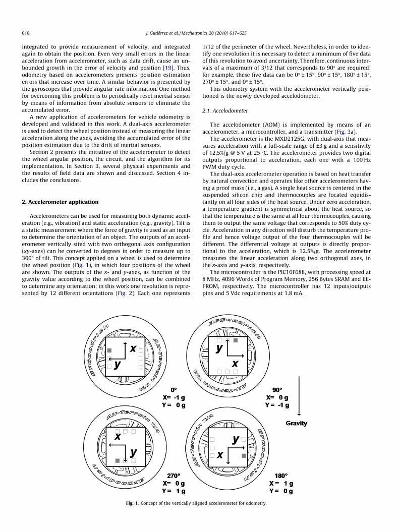
Accelerometers can be used for measuring both dynamic accel-eration (e.g., vibration) and static acceleration (e.g., gravity). Tilt isa static measurement where the force of gravity is used as an inputto determine the orientation of an object. The outputs of an accel-erometer vertically sited with two orthogonal axis configuration(xy-axes) can be converted to degrees in order to measure up to360� of tilt. This concept applied on a wheel is used to determinethe wheel position (Fig. 1), in which four positions of the wheelare shown. The outputs of the x- and y-axes, as function of thegravity value according to the wheel position, can be combinedto determine any orientation; in this work one revolution is repre-sented by 12 different orientations (Fig. 2). Each one represents
Fig. 1. Concept of the vertically align
1/12 of the perimeter of the wheel. Nevertheless, in order to iden-tify one revolution it is necessary to detect a minimum of five dataof this revolution to avoid uncertainty. Therefore, continuous inter-vals of a maximum of 3/12 that corresponds to 90� are required;for example, these five data can be 0� ± 15�, 90� ± 15�, 180� ± 15�,270� ± 15�, and 0� ± 15�.
This odometry system with the accelerometer vertically posi-tioned is the newly developed accelodometer.
2.1. Accelodometer
The accelodometer (AOM) is implemented by means of anaccelerometer, a microcontroller, and a transmitter (Fig. 3a).
The accelerometer is the MXD2125G, with dual-axis that mea-sures acceleration with a full-scale range of ±3 g and a sensitivityof 12.5%/g @ 5 V at 25 �C. The accelerometer provides two digitaloutputs proportional to acceleration, each one with a 100 HzPWM duty cycle.
The dual-axis accelerometer operation is based on heat transferby natural convection and operates like other accelerometers hav-ing a proof mass (i.e., a gas). A single heat source is centered in thesuspended silicon chip and thermocouples are located equidis-tantly on all four sides of the heat source. Under zero acceleration,a temperature gradient is symmetrical about the heat source, sothat the temperature is the same at all four thermocouples, causingthem to output the same voltage that corresponds to 50% duty cy-cle. Acceleration in any direction will disturb the temperature pro-file and hence voltage output of the four thermocouples will bedifferent. The differential voltage at outputs is directly propor-tional to the acceleration, which is 12.5%/g. The accelerometermeasures the linear acceleration along two orthogonal axes, inthe x-axis and y-axis, respectively.
The microcontroller is the PIC16F688, with processing speed at8 MHz, 4096 Words of Program Memory, 256 Bytes SRAM and EE-PROM, respectively. The microcontroller has 12 inputs/outputspins and 5 Vdc requirements at 1.8 mA.
ed accelerometer for odometry.
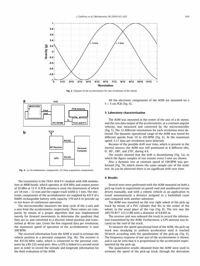
Fig. 2. Outputs of the accelerometer for one revolution of the wheel.
Fig. 3. (a) Accelodometer components. (b) Data acquisition components.
J. Gutiérrez et al. / Mechatronics 20 (2010) 617–625 619
The transmitter is the TXA1-434-F11 module with ASK modula-tion at 4800 bauds, which operates at 434 MHz and output powerof 10 dBm at 12 V. A PCB antenna is used, the dimensions of whichare 34 mm � 12 mm and the copper track width is 1 mm. The elec-tronic components of the accelodometer are supplied by 4.8 V of aNiMH rechargeable battery with capacity 170 mA h to provide upto ten hours of continuous operation.
The microcontroller measures the duty cycle of the x-axis andy-axis from the accelerometer, respectively. These values are com-pared, by means of a proper algorithm that was implementedmerely for forward movements to determine the quadrant thatthey are in, and converted to a discrete wheel position and trans-mitted at 40 ms rate. Given the five required data per revolution,the maximum speed of operation of the accelodometer is near300 RPM.
The received information from the AOM is used to estimate thevehicle position in a personal computer (Fig. 3b). The receiver isthe 433.92 MHz radio, which is connected to the personal com-puter by a RS-232 serial port. Also, a GPS is linked to a second serialport in order to record the latitude and longitude information forthe field evaluation of the AOM.
All the electronic components of the AOM are mounted on a5 � 5 cm PCB (Fig. 4).
3. Laboratory characterization
The AOM was mounted in the center of the axis of a dc motor,and the raw data output of the accelerometer, at a constant angularvelocity, was measured and converted by the microcontroller(Fig. 5). The 12 different orientations for each revolution were de-tected. The dynamic operational range of the AOM was tested fordifferent speeds from 10 to 293 RPM (Fig. 6). At the maximumspeed, 5.11 data per revolution were detected.
Because of the possible drift over time, which is present in theinertial sensors, the AOM was still positioned at 4 different tilts,0�, 90�, 180�, and 270�, during 4 h.
The results showed that the drift is dissimilating (Fig. 7a), inwhich the figure samples of one minute every 5 min are shown.
Also a dynamic test at constant speed of 100 RPM was per-formed (Fig. 7b) which shows the same sample rate of the statictest. As can be observed there is no significant drift over time.
4. Results
Several tests were performed with the AOM mounted on both apick-up truck to experiment on paved road and washboard terraindriven manually, and with a robotic vehicle as an application totravel autonomously a distance assigned in a basketball courtand compared with another odometer.
The AOM was mounted on the rear right wheel of the pick-uptruck by means of a PVC cylinder that fits in the center of thewheel, in the usual place of the cup (Fig. 8). The tire was the285/70-R17 121/118R with a diameter of 0.8305 m.
The receiver unit was onboard the truck to record the informa-tion transmitted by the AOM. Furthermore, a GPS antenna was lo-cated on the roof of the truck.
To measure the speed operational limit of the AOM, the pick-uptruck was steadying to uniform acceleration until it reached50 km/h according with the speedometer of the pick-up (Fig. 9).The frequency response of one axis of the accelerometer is shown,and it can be seen that it is proportional to the acceleration exper-imented by the pick-up.
The quantitative results obtained from the AOM were used toestimate the speed of the pick-up truck, through the derivation
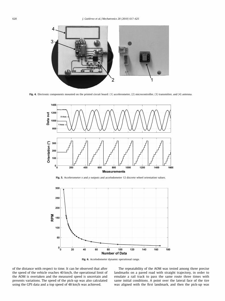
Fig. 4. Electronic components mounted on the printed circuit board: (1) accelerometer, (2) microcontroller, (3) transmitter, and (4) antenna.
Fig. 5. Accelerometer x and y outputs and accelodometer 12 discrete wheel orientation values.
Fig. 6. Accelodometer dynamic operational range.
620 J. Gutiérrez et al. / Mechatronics 20 (2010) 617–625
of the distance with respect to time. It can be observed that afterthe speed of the vehicle reaches 40 km/h, the operational limit ofthe AOM is overtaken and the measured speed is uncertain andpresents variations. The speed of the pick-up was also calculatedusing the GPS data and a top speed of 48 km/h was achieved.
The repeatability of the AOM was tested among three preciselandmarks on a paved road with straight trajectory, in order toemulate a rail track to pass the same route three times withsame initial conditions. A point over the lateral face of the tirewas aligned with the first landmark, and then the pick-up was
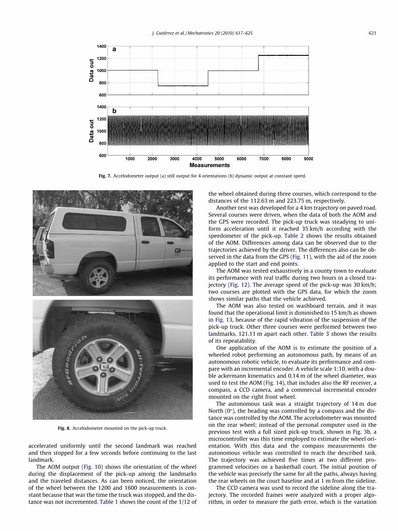
Fig. 7. Accelodometer output (a) still output for 4 orientations (b) dynamic output at constant speed.
Fig. 8. Accelodometer mounted on the pick-up truck.
J. Gutiérrez et al. / Mechatronics 20 (2010) 617–625 621
accelerated uniformly until the second landmark was reachedand then stopped for a few seconds before continuing to the lastlandmark.
The AOM output (Fig. 10) shows the orientation of the wheelduring the displacement of the pick-up among the landmarksand the traveled distances. As can been noticed, the orientationof the wheel between the 1200 and 1600 measurements is con-stant because that was the time the truck was stopped, and the dis-tance was not incremented. Table 1 shows the count of the 1/12 of
the wheel obtained during three courses, which correspond to thedistances of the 112.63 m and 223.75 m, respectively.
Another test was developed for a 4 km trajectory on paved road.Several courses were driven, when the data of both the AOM andthe GPS were recorded. The pick-up truck was steadying to uni-form acceleration until it reached 35 km/h according with thespeedometer of the pick-up. Table 2 shows the results obtainedof the AOM. Differences among data can be observed due to thetrajectories achieved by the driver. The differences also can be ob-served in the data from the GPS (Fig. 11), with the aid of the zoomapplied to the start and end points.
The AOM was tested exhaustively in a county town to evaluateits performance with real traffic during two hours in a closed tra-jectory (Fig. 12). The average speed of the pick-up was 30 km/h;two courses are plotted with the GPS data, for which the zoomshows similar paths that the vehicle achieved.
The AOM was also tested on washboard terrain, and it wasfound that the operational limit is diminished to 15 km/h as shownin Fig. 13, because of the rapid vibration of the suspension of thepick-up truck. Other three courses were performed between twolandmarks, 121.11 m apart each other. Table 3 shows the resultsof its repeatability.
One application of the AOM is to estimate the position of awheeled robot performing an autonomous path, by means of anautonomous robotic vehicle, to evaluate its performance and com-pare with an incremental encoder. A vehicle scale 1:10, with a dou-ble ackermann kinematics and 0.14 m of the wheel diameter, wasused to test the AOM (Fig. 14), that includes also the RF receiver, acompass, a CCD camera, and a commercial incremental encodermounted on the right front wheel.
The autonomous task was a straight trajectory of 14 m dueNorth (0�), the heading was controlled by a compass and the dis-tance was controlled by the AOM. The accelodometer was mountedon the rear wheel; instead of the personal computer used in theprevious test with a full sized pick-up truck, shown in Fig. 3b, amicrocontroller was this time employed to estimate the wheel ori-entation. With this data and the compass measurements theautonomous vehicle was controlled to reach the described task.The trajectory was achieved five times at two different pro-grammed velocities on a basketball court. The initial position ofthe vehicle was precisely the same for all the paths, always havingthe rear wheels on the court baseline and at 1 m from the sideline.
The CCD camera was used to record the sideline along the tra-jectory. The recorded frames were analyzed with a proper algo-rithm, in order to measure the path error, which is the variation
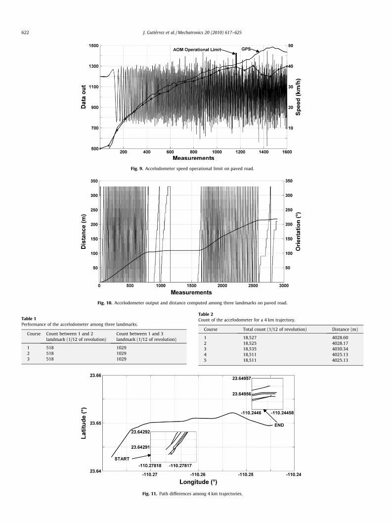
Fig. 9. Accelodometer speed operational limit on paved road.
Fig. 10. Accelodometer output and distance computed among three landmarks on paved road.
Table 1Performance of the accelodometer among three landmarks.
Course Count between 1 and 2landmark (1/12 of revolution)
Count between 1 and 3landmark (1/12 of revolution)
1 518 10292 518 10293 518 1029
Table 2Count of the accelodometer for a 4 km trajectory.
Course Total count (1/12 of revolution) Distance (m)
1 18,527 4028.602 18,525 4028.173 18,535 4030.344 18,511 4025.135 18,511 4025.13
Fig. 11. Path differences among 4 km trajectories.
622 J. Gutiérrez et al. / Mechatronics 20 (2010) 617–625
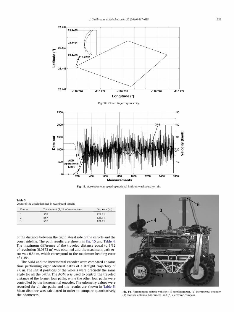
Fig. 12. Closed trajectory in a city.
Fig. 13. Accelodometer speed operational limit on washboard terrain.
Table 3Count of the accelodometer in washboard terrain.
Course Total count (1/12 of revolution) Distance (m)
1 557 121.112 557 121.113 557 121.11
Fig. 14. Autonomous robotic vehicle: (1) accelodometer, (2) incremental encoder,(3) receiver antenna, (4) camera, and (5) electronic compass.
J. Gutiérrez et al. / Mechatronics 20 (2010) 617–625 623
of the distance between the right lateral side of the vehicle and thecourt sideline. The path results are shown in Fig. 15 and Table 4.The maximum difference of the traveled distance equal to 1/12of revolution (0.0373 m) was obtained and the maximum path er-ror was 0.34 m, which correspond to the maximum heading errorof 1.39�.
The AOM and the incremental encoder were compared at sametime performing eight identical paths of a straight trajectory of7.6 m. The initial positions of the wheels were precisely the sameangle for all the paths. The AOM was used to control the traveleddistance of the former four paths, while the other four paths werecontrolled by the incremental encoder. The odometry values wererecorded for all the paths and the results are shown in Table 5.Mean distance was calculated in order to compare quantitativelythe odometers.
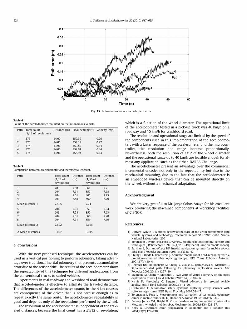
Fig. 15. Autonomous robotic vehicle path error.
Table 4Count of the accelodometer mounted on the autonomous vehicle.
Path Total count(1/12 of revolution)
Distance (m) Final heading (�) Velocity (m/s)
1 375 14.00 359.39 0.262 375 14.00 359.19 0.273 374 13.96 359.80 0.344 375 14.00 358.61 0.345 374 13.96 358.94 0.33
Table 5Comparison between accelodometer and incremental encoder.
Path Total count(1/12 ofrevolution)
Distance(m)
Total count(1/50 ofrevolution)
Distance(m)
1 203 7.58 861 7.712 204 7.61 857 7.683 204 7.61 865 7.754 203 7.58 860 7.70
Mean distance 1 7.595 7.71
5 204 7.61 853 7.646 203 7.58 852 7.637 204 7.61 860 7.708 204 7.61 859 7.69
Mean distance 2 7.602 7.665
D Mean distances 0.007 0.045
624 J. Gutiérrez et al. / Mechatronics 20 (2010) 617–625
5. Conclusions
With the new proposed technique, the accelerometers can beused in a vertical positioning to perform odometry, taking advan-tage over traditional inertial odometry that presents accumulativeerror due to the sensor drift. The results of the accelodometer showthe repeatability of this technique for different applications, fromthe conventional trucks to scaled vehicles.
Experiments in real roadway and washboard road demonstratethat accelodometer is effective to estimate the traveled distance.The differences of the accelodometer counts in the 4 km coursesare consequence of the driver that is not precise enough as torepeat exactly the same route. The accelodometer repeatability isgood and depends only of the revolutions performed by the wheel.
The resolution of the accelodometer is independent of the trav-eled distances, because the final count has a ±1/12 of revolution,
which is a function of the wheel diameter. The operational limitof the accelodometer tested in a pick-up truck was 40 km/h on aroadway and 15 km/h for washboard road.
The resolution and operational range are limited by the speed ofthe components used in this implementation of the accelodome-ter; with a faster response of the accelerometer and the microcon-troller, the resolution and range increase proportionally.Nevertheless, both the resolution of 1/12 of the wheel diameterand the operational range up to 40 km/h are feasible enough for al-most any application, such as the urban DARPA Challenge.
The accelodometer present an advantage over the commercialincremental encoder not only in the repeatability but also in themechanical mounting, due to the fact that the accelodometer isan embedded wireless device that can be mounted directly onthe wheel, without a mechanical adaptation.
Acknowledgment
We are very grateful to Mr. Jorge Cobos Anaya for his excellentwork producing the machined components at workshop facilitiesof CIBNOR.
References
[1] Durrant-Whyte H. A critical review of the state-of-the-art in autonomous landvehicle systems and technology. Technical Report SAND2001-3685. SandiaNational Laboratories; 2001.
[2] Borenstein J, Everett HR, Feng L, Wehe D. Mobile robot positioning: sensors andtechniques. J Robotic Syst 1997;14(4):231–49 [special issue on mobile robots].
[3] Barshan B, Durrant-Whyte HF. Inertial navigation systems for mobile robots.IEEE Trans Robotics Automat 1995;11(3):328–42.
[4] Chung H, Ojeda L, Borenstein J. Accurate mobile robot dead-reckoning with aprecision-calibrated fiber optic gyroscope. IEEE Trans Robotics Automat2001;17(1):80–4.
[5] Helmick DM, Roumeliotis SI, Cheng Y, Clouse D, Bajracharya M, Matthies L.Slip-compensated path following for planetary exploration rovers. AdvRobotics 2006;20(11):1257–80.
[6] Maimone M, Cheng Y, Matthies L. Two years of visual odometry on the marsexploration rovers. J Field Robotics 2007;24(3):169–86.
[7] Nistér D, Naroditsky O, Bergen J. Visual odometry for ground vehicleapplications. J Field Robotics 2006;23(1):3–20.
[8] Gustafsson F. Automotive safety systems: replacing costly sensors withsoftware algorithms. IEEE Signal Proc Mag 2009:32–47.
[9] Borenstein J, Feng L. Measurement and correction of systematic odometryerrors in mobile robots. IEEE J Robotics Automat 1996;12(6):869–80.
[10] Cooney JA, Xu WL, Bright G. Visual dead-reckoning for motion control of aMecanum-wheeled mobile robot. Mechatronics 2004;14(6):623–37.
[11] Kelly A. Linearized error propagation in odometry. Int J Robotics Res2004;23(2):179–218.

J. Gutiérrez et al. / Mechatronics 20 (2010) 617–625 625
[12] Ippoliti G, Jetto L, Longhi S. Localization of mobile robots: development andcomparative evaluation of algorithms based on odometric and inertial sensors.J Robotic Syst 2005;22(12):725–35.
[13] Borenstein J, Feng L. Gyrodometry: a new method for combining data fromgyros and odometry in mobile robots. In: Proceedings of the 1996 IEEEinternational conference on robotics and automation; 1996. p. 423–8.
[14] Foresti GL, Regazzoni CS. Multisensor data fusion for autonomous vehiclenavigation in risky environments. IEEE Trans Vehicular Technol2002;51(5):1165–85.
[15] Song X, Wang Y. A novel model-based method for odometry calculation of all-terrain mobile robots. In: Proceedings of the 7th world congress on intelligentcontrol and automation; 2008.
[16] Wang W, Wang D. Land vehicle navigation using odometry/INS/visionintegrated system. In: IEEE conference on cybernetics and intelligentsystems; 2008. p. 754–9.
[17] Thrun S, Montemerlo M, Dahlkamp H, Stavens D, Aron A, Diebel J, et al. Stanley,the robot that won the DARPA grand Challenge. J Field Robotics2006;23(9):661–92.
[18] Urmson C, Anhalt J, Bae H, Bagnell JA, Baker C, Bittner RE, et al. Autonomousdriving in urban environments: Boss and the Urban Challenge. J Field Robotics2008;25(8):425–66.
[19] Hugh HSL, Grantham KHP. Accelerometer for mobile robot positioning. IndAppl 2001;37(3):131–7.