Point-to-point trajectory planning of wheeled mobile manipulators with stability constraint....

European Journal of Mechanics A/Solids 28 (2009) 477–493

Contents lists available at ScienceDirect

European Journal of Mechanics A/Solids

www.elsevier.com/locate/ejmsol

Point-to-point trajectory planning of wheeled mobile manipulators with stabilityconstraint. Extension of the random-profile approach

M. Haddad ∗, S. Hanchi, H.E. Lehtihet

Laboratory of Structure Mechanics, E.M.P., BP 17, Bordj El-Bahri 16111, Algiers, Algeria

a r t i c l e i n f o a b s t r a c t

Article history:Received 6 March 2007Accepted 11 June 2008Available online 26 September 2008

Keywords:Mobile manipulatorTrajectory planningStability constraintStochastic optimization

We propose a flexible stochastic scheme for point-to-point trajectory planning of nonholonomic wheeledmobile manipulators subjected to move in a structured workspace. The problem is known to becomplex, particularly if obstacles are present and if dynamic stability constraint is considered. Theproposed method consists of extending to wheeled mobile manipulators the random-profile approachrecently applied to wheeled platforms. This versatile method handles constraints on: (i) geometry(obstacle avoidance, bounded joint positions and path curvature); (ii) kinematics (bounded velocities andaccelerations); (iii) dynamics (bounded torques, stability condition). It may be applied using various formsof cost functions involving travel time, efforts and power. Solutions are presented for planar and spatialnonholonomic wheeled mobile manipulators undertaking, in a constrained workspace, a point-to-pointtask defined either in generalized or operational coordinates.

© 2008 Elsevier Masson SAS. All rights reserved.

1. Introduction

A Wheeled Mobile Manipulator (WMM) typically consists of arobotic manipulator mounted on a mobile platform. Such a system,which is usually characterized by a high degree of redundancy,combines the manipulability of a fixed-base manipulator with themobility of a wheeled platform. Accordingly, it is able to accom-plish complicated tasks in large workspaces that may include manyobstacles.

Due to numerous potential applications, planning a point-to-point task for a WMM has been an important problem that hasgiven rise to much attention. Two main topics may be distin-guished: path planning and trajectory planning. The former onlydeals with the search of a time-independent continuous sequenceof configurations, taking into account geometric constraints relatedto the robot itself or to any obstacle that may be present in theworkspace. The latter topic further deals with the time history ofsuch a sequence, taking into account kinematics and dynamics. Asto the type of point-to-point tasks, three categories may be distin-guished according to the information available at the boundaries:

1. the Generalized Point-to-Point (GPP) task, for known ini-tial/final configurations;

2. the Operational Point-to-Point (OPP) task, for known ini-tial/final end-effector’s states;

* Corresponding author.E-mail addresses: [email protected] (M. Haddad),

[email protected] (H.E. Lehtihet).

3. the Modified Point-to-Point (MPP) task, for known initial con-figuration and final state.

In practice, the third category often replaces the second as theinitial configuration is usually given (Foulon et al., 1998).

In this paper, we focus on the optimal point-to-point trajectoryproblem for nonholonomic WMMs, while considering constraintson:

• geometry (obstacle avoidance, bounded path curvature, bound-ed joint positions);

• kinematics (bounded velocities, bounded accelerations);• dynamics (bounded torques, stability considerations).

The method we propose consists of extending to WMMs theRandom-Profile Approach (RPA) that was applied in Haddad et al.(2005, 2007a) to the relatively more restricted case of an iso-lated wheeled platform. As the main development has been de-tailed already in the above-cited 2007 reference, we will be con-cerned principally by the newly introduced complications thatare due, of course, to the adding of the arms but also to thehandling of stability. This latter issue cannot be safely ignoredin the case of a WMM, particularly when travel time is mini-mized. Here, stability will be considered using the zero-moment-point condition (Vukobratovic et al., 1970; Takanishi et al., 1989;Huang et al., 2000; Kim et al., 2002).

The RPA was initially proposed in Chettibi and Lehtihet (2002)in the context of fixed-base manipulators. Although it is expectedto yield sub-optimal results, the RPA is a remarkably flexible tech-

0997-7538/$ – see front matter © 2008 Elsevier Masson SAS. All rights reserved.doi:10.1016/j.euromechsol.2008.06.008

http://www.ScienceDirect.com/

http://www.elsevier.com/locate/ejmsol

mailto:[email protected]

mailto:[email protected]

http://dx.doi.org/10.1016/j.euromechsol.2008.06.008

478 M. Haddad et al. / European Journal of Mechanics A/Solids 28 (2009) 477–493

nique that involves inverse dynamics only. It remains applica-ble in various types of trajectory problems (including those withdiscontinuous dynamic models or those with electromechanicalconstraints) and with various types of optimization criteria thatmay include travel time, efforts and power. The RPA builds time-scaled trajectory profiles (Hollerbach, 1983) to map real trajectoriesover the unit interval. Next, it converts kinodynamic constraintsto bounds on the time of travel. Then, it reduces the trajectoryproblem to a constrained-profile optimization that is subsequentlysolved via a stochastic scheme. Moreover, as trajectory profiles areconveniently partitioned into motion and path components, theRPA handles separately the issue of obstacle avoidance and is ableto take full advantage of well-established probabilistic roadmaptechniques during its initialization phase.

The numerical results we describe in the last section of thispaper have been obtained by implementing the RPA using thesimulated-annealing technique of optimization (Kirkpatrick et al.,1983; Hajek, 1985). Several examples are presented for planar andspatial WMMs undertaking GPP and MPP tasks in constrainedworkspaces. One particular example, which uses a simple 1-linkWMM, offers a comparison between the solution obtained by theproposed RPA and that obtained via a technique based on Pon-tryagin’s Maximum Principle (PMP) (Pontryagin et al., 1965).

2. Related work

Most of the techniques that treat the point-to-point path-planning problem take advantage of the kinematic redundancy ofthe WMM to make the system reach configurations satisfying staticoptimization criteria that only depend on the sequence of con-figurations (generalized Euclidian distance, manipulability. . .). InCarriker et al. (1990, 1991) and in Zhao et al. (1992), the path-planning problem for multiple point-to-point tasks was formulatedas a nonlinear optimization problem. A generalized distance func-tion, representing the relative cost of moving the base and themanipulator, was minimized using stochastic techniques. In Pin etal. (1994), the path-planning problem for multiple OPP tasks wasdivided into two sub-problems: (i) forecasting the optimal commu-tation configuration for each pair of adjacent tasks and (ii) giventhe estimated initial and final configurations for each task, the pathplanning problem was formulated as a two-point boundary valueproblem. The first sub-problem was solved via the tunneling opti-mization algorithm (Levy and Gomez, 1984) using a static criterionrelated to initiating and/or finishing the tasks (best utilization ofactuator strength to lift an object and/or to maintain some maneu-verability in all directions). The second sub-problem was handledvia an approach based on Cohen’s method (Cohen, 1981), usingmulti-criteria (strength optimization, obstacle avoidance, mainte-nance of some manipulability). Foulon et al. (1998) proposed astrategy for planning point-to-point paths in both the generalizedand the operational spaces. After defining various classes of param-eterized paths, the optimal path of the nonholonomic platform wasdetermined using the redundancy of the global mechanical system.Lingelbach (2004) investigated a probabilistic cell-decompositionmethod for path planning GPP tasks while minimizing a stan-dard weighted Euclidian distance and while considering obstacleavoidance. Papadopoulos et al. (2005) proposed a method, basedon polynomial functions, yielding collision-free paths between twogiven configurations.

Several other approaches have been proposed to solve thetrajectory-planning problem for a WMM under kinematic con-straints and using criteria based on travel time and quadratic sumof velocities or accelerations. In Lee et al. (1996) and in Lee andCho (1997), the trajectory-planning problem for a WMM executinga sequence of tasks was formulated as a global-optimization prob-lem, minimizing simultaneously the quadratic sum of velocities

and the inverse of the manipulability measure. Desai et al. (1996)addressed the trajectory-planning problem for multiple nonholo-nomic WMMs using optimal-control theory. The cost function wasdefined as the integral of quadratic velocities over the history ofthe motion for a given travel time. Perrier et al. (1998) treated thetrajectory-planning problem for a WMM undertaking OPP tasks us-ing an iterative approach while considering accelerations, velocitiesand joints constraints.

In the above works, however, dynamics and stability issueshave not been considered. Hence, calculated solutions may over-take the dynamic capabilities of the system and/or induce a severeinstability of the system, particularly when travel time is mini-mized. Unfortunately, techniques able to handle trajectory prob-lems for WMMs while considering dynamics and stability con-straints are relatively few. Dubowsky and Vance (1989) addressedthe minimum-time trajectory-planning problem while consideringthe dynamics of the manipulator and the stability of the platform.However, the vehicle was considered stationary. Desai and Kumar(1997) treated the trajectory-planning problem for two cooperativemobile manipulators using optimal-control theory while consider-ing geometric and kinodynamic constraints. The cost function wasdefined as the integral of the norm of actuator forces over thehistory of the motion for a given travel time. The main disadvan-tage, however, is that the number of variables rapidly increaseswith the complexity of the problem. Watanabe et al. (1999) for-mulated the trajectory-planning problem with stability constraintas a parametric optimization problem. The cost function was de-fined as the quadratic sum of the time derivative of each jointtorque for a given travel time. However, nonholonomic constraintswere not taken into account. Mohri et al. (2001) formulated thetrajectory-planning problem as an optimal-control problem. First,they incorporated some constraints (final-state errors and obstacleavoidance constraints) as a penalty in the cost function. Then, theyapplied an iterative algorithm proposed in Iwamura et al. (2000)and based on the concept of the order of priority and the gradientfunction, which are synthesized in the hierarchical manner.

3. Dynamic model and stability condition

Let � = (O , x, y, z) be the fixed frame of the world coordi-nates. The WMM considered in this paper consists of a series-chainmulti-link manipulator mounted on a wheeled mobile platform.We assume that the motion of the platform is confined to the(O , x, y) plan and that the main part of this platform is a rigidchassis provided with nondeformable wheels. The type of the plat-form is not specified here. It may belong to any of the nonholo-nomic wheeled mobile robots discussed in Campion et al. (1996).

We note MP� = (MP O ,MP x,MP y,MP z) and EE� = (EE O ,EE x,EE y,EE z) the moving frames associated, respectively, to the mobileplatform and to the end-effectors. The operational coordinates ofthe system are described, in the most general case, by a 6-vectorU e = [xe, ye, ze, θe, βe,ϕe]T that specifies the end-effector’s statein � (Cartesian coordinates of EE O and Euler’s orientation angles ofEE� in �). The generalized coordinates of the system are describedby the n-vector q = [qT

p,qTa]T, where qp is the np-vector defin-

ing the configuration of the platform in � and qa is the na-vectordefining the configuration of the arms in MP� (so that n = np +na).

The state of the platform in � is can be described by a vec-tor U p = [xp, yp, zp, θp,0,0]T, but in our case, zp is the constantdistance between MP O and O , measured along the z-axis. Thus,the state of the platform is actually described by only the 3-vectorX p = (xp, yp, θp)T and we may write qp = [XT

p,qTw ]T, where qw

is the (np − 3)-vector of independent coordinates related to therotation/orientation of the wheels in MP�. However, as an ar-bitrary number of choices of qw may be associated to a givenend-effector’s state U e , it will be particularly useful in our case

M. Haddad et al. / European Journal of Mechanics A/Solids 28 (2009) 477–493 479

Fig. 1. Stable region and ZMP. The stable region is approximated by the largest ellipse inscribed in the WMM sustentation polygon. (a) Hexagonally-shaped sustentationpolygon; (b) Diamond-shaped sustentation polygon.

to consider the so-called partial generalized coordinates of the sys-tem (Bayle et al., 2003). These are given by the (3 + na)-vectorΩ = [XT

p,qTa]T that actually affects U e .

3.1. Dynamic model

The platform is subjected to m nonholonomic constraints(m < np) that can be written in the following compact form(Campion et al., 1991):

A(q)q̇ = 0 (1)

where A is a full-rank (m × n)-matrix. Then, using the Lagrangianapproach while considering (1), we can model the dynamics of thesystem as follows (Bloch et al., 1992):

M(q)q̈ + c(q, q̇) + g(q) = AT (q)Λ + B(q)τ . (2)

Here, M(q) is the symmetric positive-definite (n × n) inertia ma-trix. c(q, q̇) is the n-vector of centrifugal and Coriolis forces inwhich generalized velocities appear under a quadratic form. g(q)

is the n-vector of gravity forces. Λ is the m-vector of Lagrange’smultipliers associated to the m nonholonomic constraints. B(q) isa (n× (n−m)) input transformation matrix. τ is the (n−m)-vectorof external forces and torques applied to the system by the actua-tors. Expressions (1) and (2) give a full description of the dynamicsof the WMM.

Following Bloch et al. (1992), we write A(q) = [Av Au], whereAv is a m×(n−m)-matrix and Au is a nonsingular (m×m)-matrix.Next, if we define the full-rank matrix

R(q) =[

I−A−1

u Av

],

where I is the (n − m) × (n − m) identity matrix, then it followsthat A(q)R(q) = 0. Also, as the (n−m)× (n−m)-matrix RT(q)B(q)

has full rank for any feasible q (Campion et al., 1991), we may pre-multiply expression (2) by [RT(q)B(q)]−1 RT(q) to eliminate themultipliers Λ and to extract the vector τ of active-joint torques asfollows:

τ = [R T (q)B(q)

]−1R T (q)

[M(q)q̈ + c(q, q̇) + g(q)

]. (3)

3.2. Stability condition

We will treat the issue of the dynamic stability of the WMMusing the so-called Zero-Moment-Point (ZMP) condition (Vukobra-tovic et al., 1970; Takanishi et al., 1989; Huang et al., 2000). TheZMP is defined as the point on the floor under the moving plat-form where vanishes the resultant moment of gravity and inertialand external forces applied to the system.

A more complete formulation of ZMP stability criterion is givenby Kim et al. (2002). In their model, inertia effects of the rigid bod-ies are taken into account, which is very important to the systemdynamics. The ZMP coordinates can be computed by Newton–Eulerformulation as follows (Kim et al., 2002):

x0 = − N y

fzand y0 = Nx

fz. (4)

N and f are, respectively, the resultant moment and force appliedto the platform. The above coordinates are expressed in the mov-ing frame MP R ′ = (M S P ,MP x,MP y,MP z), where MSP is the MostStable Point defined as the center of the contact polygon betweenthe platform and the ground. The area enclosed in this polygon isthe stable region (Fig. 1). The system is stable as long as the ZMPbelongs to this region (Huang et al., 2000).

In most cases, WMMs have a symmetric platform (Kim et al.,2002) so that the stable region of these systems is usually approx-imated by the largest circle/ellipse inscribed in the sustentationpolygon (Fig. 1). With this simplification, the stability index Φ isdefined as follows:

Φ(q, q̇, q̈) = 1 −[(

x0

a

)2

+(

y0

b

)2](5)

where a and b are the half-diameters of the inscribed ellipse. Wenote that Φ is a dimensionless number that takes positive (neg-ative) values if the ZMP is inside (outside) the stable region. Inparticular, Φ = 0 if the ZMP is at the boundary of the stable re-gion and Φ = 1 if the ZMP coincides with the MSP.

4. Problem statement

The WMM is required to move freely from a given initial con-figuration ΩSTART = [(XS

p)T, (qSa)

T]T to a given final configuration


Fig. 2. Free-trajectory planning problem for a WMM. (a) GPP task, (b) MPP task.

ΩGOAL = [(XGp)T, (qG

a )T]T (in the case of a GPP task, Fig. 2(a)), or to

a given final end-effector’s state U GOALe = [xG

e , yGe , zG

e , θGe , βG

e ,ϕGe ]T

(in the case of an MPP task, Fig. 2(b)). In either case, we mustfind the trajectory q(t), the time history of vector τ (t) of actua-tor efforts and the travel time T so that boundary conditions arematched, all constraints are respected and a given performance in-dex is optimized.

4.1. Constraints

In addition to nonholonomic constraints (1), the set of feasi-ble trajectories is restricted by numerous other constraints thatmust be satisfied during the travel from ΩSTART to either ΩGOAL

or U GOALe . These constraints concern the boundary conditions, the

noncollision between the WMM and obstacles, the physical limita-tions on kinodynamic performances and the stability of the system.

(a) Boundary conditionsThe following conditions inherent to the achievement of the de-

sired task must be taken into account:

• Position/Orientation

Ω(t = 0) = ΩSTART and Ω(t = T ) = ΩGOAL or

U e(t = T ) = U GOALe . (6a)

• Velocity

q̇(t = 0) = 0 and q̇(t = T ) = 0. (6b)

(b) Obstacles avoidanceIf obstacles are present in the workspace then the following

constraint will hold during the motion:

Collision(q) = false (6c)

The Boolean function Collision indicates whether the WMM at con-figuration q is in collision with an obstacle or with itself.

(c) Physical limitationsAdditional constraints that may have to be verified at each in-

stant t ∈ [0, T ] represent other limitations such as those on:

• Joint positions (for example: steering angle)∣∣qi(t)∣∣ � qmax

i . (6d)

• Active-joint velocities:∣∣q̇i(t)∣∣ � q̇max

i . (6e)

• Active-joint accelerations:∣∣q̈i(t)∣∣ � q̈max

i . (6f)

• Active-joint torques:∣∣τi(t)∣∣ � τmax

i . (6g)

Here, the index i refers to the ith component of the consideredvector. Any of the above constraints may be expressed using asym-metric bounds.

(d) Stability constraintIn order to ensure the stability of the system, the ZMP must

be kept inside the stable region. Thus, at any instant t in [0, T ],the stability degree given by (5) is subjected to the following con-straint:

Φ(q(t), q̇(t), q̈(t)) � 0. (6h)

4.2. Performance index

The goal function J to be minimized represents the travel costof the calculated trajectory. The following expression is a balancebetween the travel time T and quadratic averages of actuator ef-forts E and power P :

J = (1 − α)T + α((1 − β)E + β P

). (7)

Here, E and P have the dimension of a time:

E =T∫

0

n∑i=1

wi

(τi

τmaxi

)2

dt and P =T∫

0

n∑i=1

wi

(q̇iτi

q̇maxi τmax

i

)2

dt

α and β are user-defined weight coefficients: 0 � α � 1; 0 � β � 1.The limit case α = 0 corresponds to the minimum-time problemwhereas the case α = 1 (and T fixed) corresponds (if β = 0) tothe minimum-effort problem or (if β = 1) to the minimum-powerproblem. The other coefficients wi (i = 1, . . . ,n), which appearinside the above sums, are additional user-defined weight coeffi-cients that will allow giving, if desirable, more importance to someof the active joints.


5. Proposed method (RPA)

First, we give an outline of the RPA, as used in Haddad et al.(2007a) for trajectory planning of wheeled mobile robots. Then, wewill extend this same approach to point-to-point trajectory plan-ning of WMM.

5.1. Outline

Using the following time-scaling transformation, any trajectoryq(t) can be uniquely characterized by a travel time T and a time-evolution shape Q :

q(t) = Q(ξ(t)

) = Q (ξ) ◦ ξ(t). (8)

The time-scale function is defined as ξ(t) ≡ t/T so that mean-ingful values of ξ will all be located in the unit interval. The trajec-tory profile Q (ξ) gives the shape of the time history of q from thestart of the motion (ξ = 0) to its end (ξ = 1). Hereafter, the primesymbol will be reserved exclusively to indicate derivatives with re-spect to ξ while the dot symbol will refer as usual to derivativeswith respect to t .

A profile Q may be viewed also as a trajectory template thatuniquely defines a class of trajectories, all of which having thesame shape but distinctive travel times. The key point is that,for any arbitrarily given class Q , we can apply a clipping process(that accounts for kinodynamic constraints, including stability con-straint) to extracts both the travel time T Q and the travel cost C Qof the most competitive member of this class. Namely, not only canwe easily find the best score reachable within any given class butalso we can determine the specific travel time that distinguishesits best member. Consequently, the difficult task of finding the op-timal trajectory q(t)best, with unknown travel time T best, now canbe reduced to finding only the profile Q (ξ)best of this desired tra-jectory.

The RPA strives to achieve this goal using a nested master-slaveoptimization. The slave routine is the above-mentioned clipping.Given an arbitrary input candidate profile Q , the cost function Jis rewritten in terms of the single variable T . In addition, non-tight kinodynamic constraints are rewritten in terms of boundson T . Thus, the clipping process is a straightforward technique thatsolves a one-dimensional minimization problem within the tempo-ral window(s) dictated by kinodynamic constraints. This inner-leveldeterministic optimization plays the role of a workhorse fitnessfunction that will be called repeatedly at the outer-level by a mas-ter stochastic routine. The master routine tries to find the bestclass using a simulated-annealing scheme. Its built-in Metropolisalgorithm (Hajek, 1985) randomly targets candidate classes amongthose that would most likely lead to the global minimum of thecost function. Hence, the aimed output of the RPA is the most com-petitive member of the best reachable class.

Naturally, this difficult functional optimization is converted, viaa discretization of trajectory profiles, into a more tractable finite-dimensional parametric optimization. Namely, each trial profile isdefined as a finite set of free control points; continuity is achievedby fitting a smooth model that accounts for geometric constraintsand for boundary conditions. As a result, the whole trajectoryproblem boils down to disrupting randomly the control points ofthe fitting model until finding their optimal positions.

One drawback is that the simulated-annealing scheme, althoughit is not easily attracted by poorer local extrema, may still fail tofind the global optimal solution. The major drawback, however, isthat the search space itself is restricted to the sub-space reach-able via the fitting model. In addition, if obstacles are present inthe workspace, the calculation scope will be further restricted toa user-defined corridor (see, Section 5.6). Therefore, solutions areexpected to be sub-optimal (Haddad et al., 2007a).

On the other hand, the RPA offers some interesting features.First, the exploration of the solution space is done directly at theclass level. There is no need to probe at the member level since theclipping immediately yields the best trajectory within any givenclass. Yet, the most interesting feature is the remarkable flexibilityof the proposed method.

Indeed, as any trajectory may always be written in terms of ageometric path and a motion on this path, then we may express atrajectory profile as follows:

Q (ξ) = P (λ(ξ)) = P (λ) ◦ λ(ξ). (9)

The parametric form P (λ) with λ ∈ [0,1], is a time-independentcontinuous sequence of configurations that describes completelythe geometry of the robot path in the generalized-coordinate spaceas λ varies in [0,1]. The shape of the time history of such a se-quence is given by a monotonically increasing motion functionλ(ξ). This partition path/motion is handy. First, each part maymake use of an adapted fitting model through separate sets ofcontrol nodes. Also, it is clear already that λ(ξ) will never be con-cerned by collision tests. A valid motion function must verify thefollowing conditions of consistency:

λ(ξ = 0) = 0 and λ(ξ = 1) = 1, (10a)

λ′(ξ) > 0 ∀ξ ∈ ]0,1[. (10b)

Moreover, it must match boundary conditions (6b) on the robotvelocity, namely:

λ′(ξ = 0) = 0 and λ′(ξ = 1) = 0. (10c)

As to nonholonomic constraints (1), they become from (8) and(9) as follows:

A(P )dP

dλ= 0 ∀λ ∈ [0,1]. (11)

A feasible path P (λ) must satisfy not only boundary con-ditions (6a) and geometric constraints (6c) and (6d) but alsononholonomic constraints (11). However, if we write P (λ) =[P T

p(λ), P Ta(λ)]T, where P p(λ) is the path of the platform and

P a(λ) is that of the arms, then (11) will concern P p exclusively.Now, in order to account for (11) for any λ ∈ [0,1], we fur-

ther split P p(λ) = [ P̄Tp(λ), P̃

Tp(λ)]T. For example, in the case of

a unicycle-type platform, we may define P̄ p(λ) ≡ [xp(λ), yp(λ)]T

and P̃ p(λ) ≡ [θ(λ),qTw(λ)]T. Then, for any arbitrary shape chosen

for P̄ p(λ), we can deduce the corresponding P̃ p(λ) so that (11) issatisfied systematically.

5.2. Trajectory planning of a WMM in GPP tasks

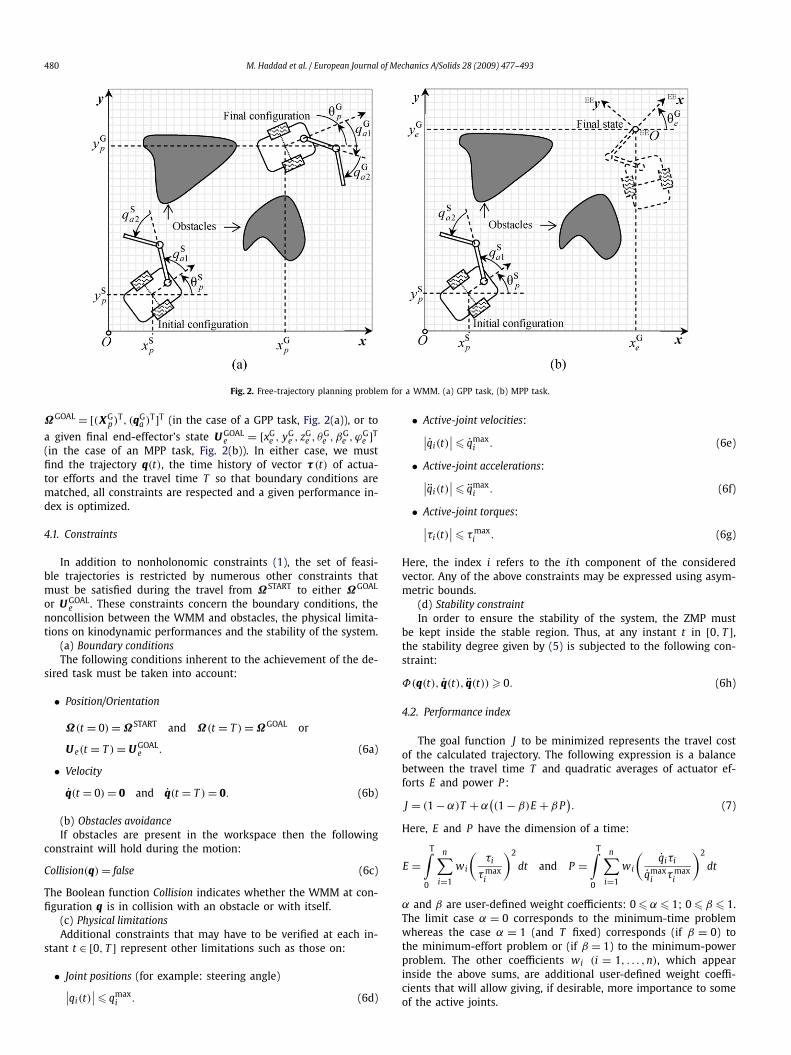
The problem is converted to a parametric optimization wherethe only unknowns are the positions of some control points. A ran-dom class Q can be built using, altogether, three distinct sets Sm ,S p and Sa of control points. Sm is made up of Nm + 2 points inthe (ξ, λ) space (Fig. 3(a)) while S p and Sa contain, respectively,N p + 4 points placed in the platform workspace (Fig. 3(b)) andNa + 2 points in the manipulator configuration space (Fig. 3(c)).

Using the first set Sm , a trial motion function can be producedby fitting a smooth curve through the Nm + 2 points of this set. Asshown in Fig. 3(a), the first and last points are held fixed accord-ing to (10a) but the Nm interior points are freely positioned whilematching (10b) and (10c). Here, a clamped cubic-spline model (i.e.,user-defined end-slopes) is well adapted to handle the first-orderboundary conditions (10c). It will also insure continuity up tosecond-order while remaining computationally efficient.

Similarly, using the other two sets S p and Sa , we can build trialpaths P̄ p(λ) and P a(λ), respectively, in the platform workspace


Fig. 3. Discretization of a trajectory profile for GPP tasks. (a) A motion profile λ(ξ) through Nm + 2 control points. (b) A platform path P̄ p(λ) through Np + 4 control points.(c) A manipulator path P a(λ) through Na + 2 control points. Free (fixed) points are shown as white (black) circles. The fixed control points insure boundary conditions.

(Fig. 3(b)) and in the manipulator configuration space (Fig. 3(c)).Here, a parametric B-spline model of order four (or higher) willbe more suitable to match boundary conditions imposed on therobot position/orientation and to insure the continuity of joint po-sitions, and later on, that of velocities, accelerations and torques.For instance, conditions (6a) on position/orientation are insured byprefixing four control points for P̄ p(λ) and two for P a(λ). Thesepoints are shown in black in Figs. 3(b) and 3(c).

In summary, the proposed random-profile approach consists ofscanning simultaneously the available solution space of Nm + N p +Na free control points of sets Sm , S p and Sa . The simplicity of thismethod resides principally in the fact that the positions of thesepoints constitute the only unknowns of the problem. As outlinedin Fig. 4, each random setting of control points will yield a trialshape for λ(ξ), P̄ p(λ) and P a(λ) from which is built a candidatetrajectory profile Q (ξ). This candidate satisfies systematically non-holonomic constraints. If, in addition, this candidate is viable (nocollision), then the clipping process is applied to evaluate its fit-ness. In other words, for each random setting of control points,we calculate a cost. This stochastic process is repeated yielding, asa final output, the optimal setting of control points and the cor-responding lowest-cost trajectory satisfying all constraints of theproblem.

5.3. Trajectory planning of a WMM in MPP tasks

For MPP tasks, the final partial configuration ΩGOAL is notgiven. This difficulty is handled by including the final configura-tion of the arms qG

a as an additional unknown of the problem.Namely, for any randomly generated qG

a (Fig. 5(a)), the final stateU G

p of the platform is deduced (Fig. 5(b)) in such a way the con-

dition imposed on the final state U GOALe of the end-effector’s is

systematically satisfied.The direct kinematics model of the WMM is given as follows

(Pin et al., 1997):

U e = U p + F (qa) (12)

where F is the kinematic transformation function of the manipu-lator (state vector of EE� in MP�). Hence, for any random choice ofqG

a , we can extract the final state of the platform as follows:

U Gp = U GOAL

e − F(qG

a

). (13)

We give next some details of implementation regarding theclipping process and the handling of the constraints of the prob-lem.

5.4. Evaluation of the performance index

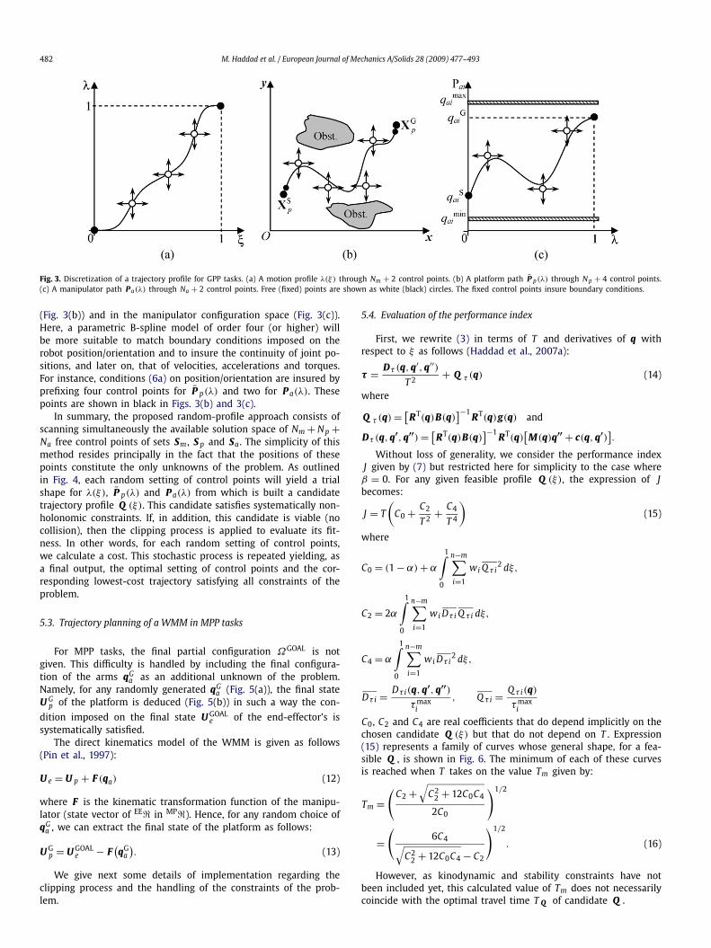
First, we rewrite (3) in terms of T and derivatives of q withrespect to ξ as follows (Haddad et al., 2007a):

τ = Dτ (q,q′,q′′)T 2

+ Q τ (q) (14)

where

Q τ (q) = [RT(q)B(q)

]−1RT(q)g(q) and

Dτ (q,q′,q′′) = [RT(q)B(q)

]−1RT(q)

[M(q)q′′ + c(q,q′)

].

Without loss of generality, we consider the performance indexJ given by (7) but restricted here for simplicity to the case whereβ = 0. For any given feasible profile Q (ξ), the expression of Jbecomes:

J = T

(C0 + C2

T 2+ C4

T 4

)(15)

where

C0 = (1 − α) + α

1∫0

n−m∑i=1

wi Q τ i2 dξ,

C2 = 2α

1∫0

n−m∑i=1

wi Dτ i Q τ i dξ,

C4 = α

1∫0

n−m∑i=1

wi Dτ i2 dξ,

Dτ i = Dτ i(q,q′,q′′)τmax

i

, Q τ i = Q τ i(q)

τmaxi

C0, C2 and C4 are real coefficients that do depend implicitly on thechosen candidate Q (ξ) but that do not depend on T . Expression(15) represents a family of curves whose general shape, for a fea-sible Q , is shown in Fig. 6. The minimum of each of these curvesis reached when T takes on the value Tm given by:

Tm =(

C2 +√

C22 + 12C0C4

2C0

)1/2

=(

6C4√C2

2 + 12C0C4 − C2

)1/2

. (16)

However, as kinodynamic and stability constraints have notbeen included yet, this calculated value of Tm does not necessarilycoincide with the optimal travel time T Q of candidate Q .


Fig. 4. Nested optimization process used by RPA. The dashed bloc is a process that generates random trajectory profiles. The fitness of each random profile Q (ξ) is evaluatedby a clipping process (that accounts for kinodynamic constraints and stability) to yield the best travel time T Q and the corresponding travel cost C Q = J Q (T Q ). The finaloutput is the best profile with the lowest cost overall. (The annealing schedule is not shown in this diagram.)


Fig. 5. Discretization of a robot path for MPP tasks. (a) A manipulator path P̄a(λ) through Na + 1 control points. (b) A platform path P̄ p(λ) through Np + 4 control points.Free (fixed) points are shown as white (black) circles. Deduced control points are shown in grey.

Fig. 6. Variations of the cost function J with T (for a given Q ).

5.5. Treatment of kinodynamic and stability constraints (clippingprocess)

Given a trial candidate Q , kinodynamic constraints (6e), (6f)and (6g) simply translate to bounds on admissible values of thetravel time T of that candidate (Chettibi and Lehtihet, 2002):

T ∈ [TLower, TUpper]. (17)

Using a straightforward chain-rule differentiation, velocity con-straints (6e) becomes:

T � T V where T V = maxi

[maxξ∈[0,1] |q′

i |q̇max

i

]. (18a)

Acceleration constraints (6f), when treated in a similar way, willgive another lower bound noted T A :

T � T A where T A = maxi

[maxξ∈[0,1] |q′′

i |q̈max

i

]1/2

. (18b)

As for torque constraints (6g), since they may be written via (14)under the form:

−τmaxi � Dτ i

T 2+ Q τ i � τmax

i , i = 1, . . . ,n − m.

So that they usually translate to bracketing bounds on T :

T ∈ [T L, T R ]. (18c)

Hence, the window (17) is deduced by simply intersecting (18a),(18b) and (18c).

The stability constraint (6h) is converted also into a set of ad-missible subintervals for T . Following Haddad et al. (2006), com-ponents Nx , N y and f z can be written as follows:⎧⎪⎪⎪⎨⎪⎪⎪⎩

Nx = DNx(q,q′,q′′)T 2 + Q Nx(q),

N y = DN y(q,q′,q′′)T 2 + Q N y(q),

f z = D f z(q,q′,q′′)T 2 + Q f z(q).

(19)

In the above expressions, the first terms represent the effect ofinertial, Coriolis and centrifugal forces while the second regroupsthe effect of gravitational and external forces. Using (4), (5) and(19), the constraint (6h) may be written under the following form:

H0 + H2

T 2+ H4

T 4� 0 (20)

where

H0 = a2b2 Q 2f z − a2 Q 2

Nx − b2 Q 2N y,

H2 = 2(a2b2 D f z Q f z − a2 DNx Q Nx − b2 DN y Q N y

),

H4 = a2b2 D2f z − a2 D2

Nx − b2 D2N y .

Hence, (20) may lead to at most two distinct intervals of admissi-ble values of T :

T ∈ [T L1, T R1] ∪ [T L2, T R2]. (21)

However, as we must intersect (17) and (21) for any ξ in [0,1], thismay yield to a set of k distinct windows: Π = [T1, T2] ∪ [T3, T4] ∪· · · ∪ [Tk−1, Tk] (Haddad et al., 2006). Consequently, for any trialcandidate Q , the corresponding optimal travel time T Q must min-imize J within Π . As to Tm given by (16) for the unconstrainedcase, it will coincide with T Q only if it belongs to Π . Otherwise,T Q will be equal to one of the Ti (i = 1, . . . ,k).

5.6. Treatment of geometric constraints

Geometric constraints such as (6c) or (6d) will not induce anyrestriction on T . In both cases, only path profiles are actually rel-evant. Any candidate P (λ) that infringes these constraints will besimply rejected since it will not lead to a feasible solution. The fol-lowing is a brief description of a pre-processing phase involvinggeometric calculations only. The purpose is to bias appropriatelythe stochastic exploration in order to make the method more ef-fective.

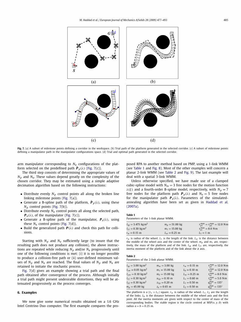
The first step consists of choosing a corridor between obstacles.As shown in Fig. 6(a), a corridor may be defined as a subset ofmilestone points in the workspace. These points, shown as crosses,can be placed manually or can be calculated by cell decompositionor probabilistic roadmap methods (Latombe, 1991), (Kavraki et al.,1996). The issue will not depend on the precise position of thesepoints but computations will be limited to the selected corridor.In other words, once a corridor is chosen, it will constitute a re-stricted search space within which the N p free control points ofthe set S p will be randomly positioned to generate trial geometricpaths P̄ p(λ) as illustrated in Fig. 7(b).

The second step consists of choosing a path P a(λ) for the arms.This path may be defined as a subset of Na configurations of the


Fig. 7. (a) A subset of milestone points defining a corridor in the workspace. (b) Trial path of the platform generated in the selected corridor. (c) A subset of milestone pointsdefining a manipulator path in the manipulator configurations space. (d) Trial and optimal path generated in the selected corridor.

arm manipulator corresponding to Na configurations of the plat-form selected on the predefined path P̄ p(λ) (Fig. 7(c)).

The third step consists of determining the appropriate values ofN p and Na . These values depend greatly on the complexity of thechosen corridor. They may be estimated using a simple adaptivedecimation algorithm based on the following instructions:

• Distribute evenly N p control points all along the broken linelinking milestone points (Fig. 7(a)).

• Generate a B-spline path of the platform, P̄ p(λ), using theseN p control points (Fig. 7(b)).

• Distribute evenly Na control points all along the selected path,P a(λ), of the manipulator (Fig. 7(c)).

• Generate a B-spline path of the manipulator, P a(λ), usingthese Na control points (Fig. 7(d)).

• Build the generalized path P (λ) and check this path for colli-sions.

Starting with N p and Na sufficiently large (to insure that theresulting path does not produce any collision), the above instruc-tions are repeated while reducing N p and/or Na progressively untilone of the following conditions is met: (i) it is no longer possibleto produce a collision-free path or (ii) user-defined minimum val-ues of N p and Na are reached. The final values of N p and Na areretained to initiate the stochastic process.

Fig. 7(d) gives an example showing a trial path and the finalpath obtained after convergence of the process. Although initiallya trial path might present undesirable distortions, they will be at-tenuated progressively as the process converges.

6. Examples

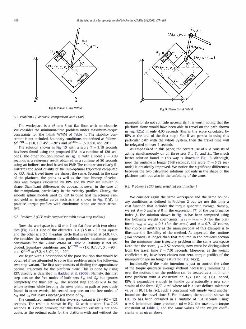
We now give some numerical results obtained on a 1.6 GHzIntel Centrino Duo computer. The first example compares the pro-

posed RPA to another method based on PMP, using a 1-link WMM(see Table 1 and Fig. 8). Most of the other examples will concern aplanar 2-link WMM (see Table 2 and Fig. 9). The last example willdeal with a spatial 3-link WMM.

Unless otherwise specified, we have made use of a clampedcubic-spline model with Nm = 3 free nodes for the motion functionλ(ξ) and a fourth-order B-spline model, respectively, with N p = 7free nodes for the platform path P p(λ) and Na = 5 free nodesfor the manipulator path P a(λ). Parameters of the simulated-annealing algorithm have been set as given in Haddad et al.(2007a).

Table 1Parameters of the 1-link planar WMM.

Izp = 3.475 kg m2 mp = 51.00 kg τmaxp1 = τmax

p2 = 12.0 N m

Iz1 = 0.30 kg m2 m1 = 15.00 kg τmaxa1 = 8.0 N m

rw = 0.15 m Lw = 0.25 m L1 = 1 m

rw is radius of the wheel. L1 is the length of the link. Lw is the distance betweenthe middle of the wheel axis and the center of the wheel. mp and m1 are, respec-tively, the mass of the platform and of the link. Izp and Iz1 are, respectively, theinertia moment of the platform and of the link about the z axis.

Table 2Parameters of the 2-link planar WMM.

Izp = 3.00 kg m2 mw = 3.00 kg rw = 0.15 m τmaxp1 = 12.0 N m

Izw = 0.05 kg m2 m1 = 15.00 kg Lb = 0.10 m τmaxp2 = 12.0 N m

I yw = 0.10 kg m2 m2 = 15.00 kg Lw = 0.25 m τmaxa1 = 8.0 N m

Iz1 = 0.30 kg m2 xGp = 0.10 m Lv = 0.60 m τmaxa2 = 5.0 N m

Iz2 = 0.30 kg m2 zGp = 0.20 m L1 = 0.50 m qmaxa1 = 135◦

mp = 45.00 kg za = 0.65 m L2 = 0.50 m qmaxa2 = 135◦

The platform is a (Lv × Lv ) square. rw is radius of the wheel. L1, L2 are the lengthof the links. Lb is the distance between the middle of the wheel axis and the firstjoint. All the inertia moments are given with respect to the center of mass of thecorresponding bodies. The stable region is the circle centred at MSP(x, y,0) withradius a = b = 0.25 m.


Fig. 8. Planar 1-link WMM.

6.1. Problem 1 (GPP task: comparison with PMP)

The workspace is a (6 m × 6 m) flat floor with no obstacle.We consider the minimum-time problem under maximum-torqueconstraints for the 1-link WMM of Table 1. The stability con-straint is not included. Boundary conditions are defined as follows:ΩSTART = (1.0,1.0,45◦,−20◦) and ΩGOAL = (5.0,5.0,45◦,20◦).

The solution shown in Fig. 10 with a score T = 3.16 secondshas been found using the proposed RPA in a runtime of 120 sec-onds. The other solution shown in Fig. 11 with a score T = 3.09seconds is a reference result obtained in a runtime of 80 secondsusing an indirect method based on PMP. The comparison clearly il-lustrates the good quality of the sub-optimal trajectory computedby RPA. First, travel times are almost the same. Second, in the caseof the platform, the paths as well as the time history of veloc-ities and torques calculated by RPA and by PMP are similar inshape. Significant differences do appear, however, in the case ofthe manipulator, particularly in the velocity profiles. Clearly, thesmooth spline models used by RPA to build trial trajectories can-not yield an irregular curve such as that shown in Fig. 11(d). Inpractice, torque profiles with continuous slope are more attrac-tive.

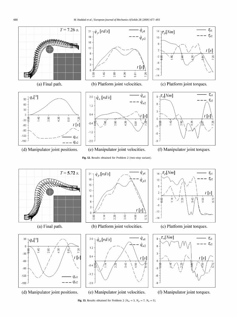
6.2. Problem 2 (GPP task: comparison with a two-step variant)

Now, the workspace is a (8 m × 7 m) flat floor with two obsta-cles (Fig. 12(a)). One of the obstacles is a (3.5 m × 3.5 m) squareand the other is a 0.5 m-radius circle that is centered at (4.0,4.0).We consider the minimum-time problem under maximum-torqueconstraints for the 2-link WMM of Table 2. Stability is not in-cluded. Boundary conditions are: ΩSTART = (1.0,0.7,0◦,0◦,−90◦)and ΩGOAL = (7.2,4.5,0◦,0◦,−90◦).

We begin with a description of the poor solution that would beobtained if we attempted to solve this problem using the followingtwo-step variant. The first step consists of finding the approximateoptimal trajectory for the platform alone. This is done by usingRPA directly as described in Haddad et al. (2006). Namely, this firststep acts on the free nodes of both sets Sm and S p but ignorescompletely the third set Sa . The second step applies RPA to thewhole system while keeping the same platform path as previouslyfound. In other words, this second step acts on the free nodes ofSm and Sa but leaves unchanged those of S p .

The cumulated runtime of this two-step variant is 29+92 = 121seconds. The result is shown in Fig. 12 with a score T = 7.26seconds. It is clear, however, that this two-step variant is not ade-quate, as the optimal paths for the platform with and without the

Fig. 9. Planar 2-link WMM.

manipulator do not coincide necessarily. It is worth noting that theplatform alone would have been able to travel on the path shownin Fig. 12(a) in only 4.05 seconds (this is the score calculated byRPA at the end of the first step). Yet, if we persist in using thisparticular path with the whole system, then the travel time willbe relegated to over 7 seconds.

As emphasized in this paper, the correct use of RPA consists ofacting simultaneously on all three sets Sm , S p and Sa . The muchbetter solution found in this way is shown in Fig. 13. Although,now, the runtime is longer (148 seconds), the score (T = 5.72 sec-onds) is drastically improved. We notice the significant differencesbetween the two calculated solutions not only in the shape of theplatform path but also in the unfolding of the arms.

6.3. Problem 3 (GPP task: weighted cost function)

We consider again the same workspace and the same bound-ary conditions as defined in Problem 2 but we use this time acost function that includes the torque quadratic average. Namely,we set β = 0 and α = 0 in the expression (7) of the performanceindex J . The solution shown in Fig. 14 has been computed usingthe following weight coefficients: w P 1 = w P 2 = 0 (for the plat-form), wa1 = wa2 = 0.5 (for the arms) and α = 0.7. Of course,this choice is arbitrary as the main purpose of this example is toillustrate the flexibility of the method. As expected, the runtime(164 seconds) is longer than that required in the previous sectionfor the minimum-time trajectory problem in the same workspaceNote that the score, J = 2.57 seconds, now must be distinguishedfrom the travel time T = 7.01 seconds. Moreover, as the weightcoefficients wa have been chosen non zero, torque profiles of themanipulator are no longer saturated (Fig. 14(c)).

Incidentally, if the main intention is just to control the valueof the torque quadratic average without necessarily minimizing itover the motion, then the problem can be treated as a minimum-time problem with a constraint on E/T (see Eq. (7)). Indeed,RPA is expandable enough to handle quite naturally a new con-straint of the form: E/T < tol, where tol is a user-defined tolerancevalue in [0,1]. In fact, such a constraint will simply yield anotherbound on the travel time T . For instance, the solution shown inFig. 15 has been obtained in a runtime of 161 seconds using:α = 0 (minimum-time problem), tol = 0.2, the maximum-torqueconstraint of Table 2, and the same values of the weight coeffi-cients w as given above.


Fig. 10. Results obtained by RPA for Problem 1. Fig. 11. Results obtained by PMP for Problem 1.


Fig. 12. Results obtained for Problem 2 (two-step variant).

Fig. 13. Results obtained for Problem 2 (Nm = 3, N p = 7, Na = 5).




6.4. Problem 4 (GPP task: introduction of the stability constraint)

The workspace is a (8 m × 8 m) flat floor with two iden-tical triangular obstacles (Fig. 16(a)). Boundary conditions aredefined as follows: ΩSTART = (1.3,2.3,0◦,0◦,90◦) and ΩGOAL =(2.0,7.0,135◦,90◦,−90◦). We consider the minimum-time prob-lem under maximum-torque constraints for the 2-link WMM.

The solution shown in Fig. 16 with a score T = 5.99 secondshas been found in a runtime of 152 seconds without consideringthe issue of stability. Accordingly (see Fig. 16(b)), if the systemshould follow this particular trajectory then the ZMP will not bekept within the Boundary of Stable Region (BSR), symbolized inthis figure by a dashed circle. The other solution shown in Fig. 17,has been computed for the same problem while including the sta-bility constraint. As expected, the new score is poorer (T = 6.47seconds). Moreover, the runtime (178 seconds) is longer becauseof the additional computational load. On the other hand, the ZMPstays within the BSR throughout the motion (Fig. 17(b)).

6.5. Problem 5 (MPP task)

We consider again the previous problem using the same ini-tial configuration ΩSTART, but we now require the system to moveto a final end-effector’s state U G

e . Note that this final state ischosen to be compatible with the final configuration ΩGOAL ofthe previous example so that results can be compared. Note alsothat calculations now are carried out using Na = 6 (instead of 5)free nodes for the path of the manipulator. Two distinct versions(A and B) of this problem are considered. In version A, the finalestate is defined completely: U G

e = (1.222,7.071,0.65,135◦,0◦,0◦)while in version B it is only partly defined in the sense thatthe end-effector’s final orientation is left unspecified: U G

e =(1.222,7.071,0.65, free,0◦,0◦).

The solutions calculated by RPA for both versions, while con-sidering stability, are shown in Fig. 18. The runtimes are approx-imately the same (187 seconds). In both cases, the ZMP is keptwithin the BSR (not shown). Comparing the two runs, we clearlynotice the significant difference in the platform paths and the op-posite unfolding of the arms. As the end-effector’s goal orientationis not imposed in version B, the RPA was able to take advantage ofthis extra freedom by choosing a faster path for the platform butalso by determining the proper unfolding of the arms to compen-sate the platform inertia forces. As a result, the score of version B(T = 6.24 seconds) is slightly improved comparatively to that ofversion A (T = 6.45 seconds).

It is interesting to observe that, in both versions of the prob-lem, the calculated solution does not tend towards reducing thelength l of the platform path. This result somewhat disagrees withthe first step of the method proposed in Foulon et al. (1998), andwhich consists of forecasting the approximate final position of theplatform by minimizing l. On the other hand, if stability is not in-cluded then calculations no longer seem to contradict the approachproposed in the above-cited reference. This is clearly apparent inFig. 19 that gives, for both versions of the problem, the solutionsobtained without considering stability. We notice the importantstretching of the arms and the resulting set back position of theplatform near the end of the motion.

6.6. Problem 6 (GPP task: long corridor)

The purpose of this example is to illustrate the behavior ofRPA when the number of free nodes is increased. The workspaceis a (11 m × 10 m) flat floor with several obstacles (Fig. 20).We consider the minimum-time problem for the 2-link WMMwith constraints on maximum torques and on stability. Boundaryconditions are: ΩSTART = (0.8,4.5,90◦,−90◦,90◦) and ΩGOAL =(0.8,7.2,−90◦,90◦,−90◦). The solution shown in Fig. 20 has been


Fig. 16. Results obtained for Problem 4 without stability constraint (Nm = 3, N p = 7,Na = 5).

Fig. 17. Results obtained for Problem 4 with stability constraint (Nm = 3, N p = 7,Na = 5).


Fig. 18. Results obtained for Problem 5 with stability constraint (Nm = 3, N p = 7, Na = 6). (a) The end-effector’s goal orientation is imposed. (b) The end-effector’s goalorientation is free.

Fig. 19. Results obtained for Problem 5 without stability constraint (Nm = 3, Np = 7, Na = 6). (a) The end-effector’s goal orientation is imposed. (b) The end-effector’s goalorientation is free.

Fig. 20. Result obtained for Problem 6. (Nm = 3, N p = 32, Na = 32).

calculated by RPA using Nm = 3 and N p = Na = 32. It has requireda runtime of 22 minutes. We note that the arm manipulator is gen-erally oriented towards the center turn of the path; this is in orderto compensate, by the weight of the arm manipulator, the influ-ence of the centrifugal force on the dynamic stability of the robot.

6.7. Problem 7 (GPP task: spatial WMM)

We consider the minimum-time trajectory problem with con-straints on maximum torque and on stability for the spatial 3-linkWMM (Fig. 21) whose characteristics are listed in Table 3. The plat-


Fig. 21. Spatial 3-link WMM.

Table 3Parameters of the 3-link WMM.

J α j

[◦]L j

[m]r j

[m]θ j

[◦]m j

[kg]xG j

[m]zG j

[m]Ix j

[kg m2]I y j

[kg m2]I z j

[kg m2]qmax

j[◦]

τmaxj

[N m]

1 0 0.1 1.0 qa1 20.0 0.00 −0.30 0.120 135 20.02 −90 0.0 0.0 qa2 7.0 0.25 0.00 0.003 0.020 0.020 80 45.03 0 0.5 0.0 qa3 5.0 0.25 0.00 0.002 0.010 0.010 120 20.0

form is the same as that of the planar WMM shown in Fig. 9.The only difference concerns the maximum torques (which noware fixed as follows: τmax

p1 = τmaxp2 = 20 N m). All inertia moments

are given with respect to the center of mass of the correspondingbodies. The moving frames attached to the rigid bodies of the ma-nipulator are defined using the Khalil–Kleinfinger method (Khaliland Dombre, 2002).

The workspace is a (6 m × 6 m) flat floor with one obstacle(Fig. 22(a)). Boundary conditions are defined as follows: ΩSTART =(1,0.5,90◦,90◦,−45◦,45◦) and ΩGOAL = (3.5,5.5,90◦,90◦,0◦,0◦).The solution shown in Fig. 22 with a score T = 3.53 seconds hasbeen calculated by RPA in a runtime of 272 seconds. If stability isnot included, the score will be T = 3.45 seconds and will requirea runtime of 235 seconds.

We note that the arm manipulator is generally folded down-wards in order to lower the center of gravity of the robot and todecrease the influence of inertia forces on the dynamic stability.

7. Conclusion

In this work, we have proposed an extension of the random-profile approach to handle trajectory-planning problems of WMMs,in GPP and MPP tasks, while considering kinodynamic constraintsand obstacle avoidance. The cost function has been written in aconvenient weighted form that may include travel time, efforts andpower. In this extension, we have:

(i) Considered the trajectory-planning problem of a WMM in aGPP task. This has required searching simultaneously for thetrajectory of the platform and that of the arm manipulator.Comparatively to the case of a platform alone, this problem ischaracterized by a much stronger nonlinearity, due to the dy-namic coupling platform/arm, and by a broader search space,due to a high degree of redundancy.

(ii) Considered the trajectory-planning problem of a WMM in anMPP task. This has required dealing with the additional diffi-culty due to the unknown final configuration of the WMM.

(iii) Considered the issue of stability by a transforming this con-straint to a set of admissible subintervals for the travel time.

Fig. 22. Results obtained for Problem 7 with stability constraint (Nm = 3, N p = 7, Na = 5).


Further extensions of RPA are possible to handle the followingspecial cases: (a) the end-effector’s path is specified or (b) the plat-form of the WMM is under-actuated. Preliminary results are given,respectively, in Haddad et al. (2007b, 2008).

References

Bayle, B., Fourquet, J.-Y., Renaud, M., 2003. From manipulation to wheeled mobilemanipulation: analogies and differences. In: 7th Symposium on Robot Control(SYROCO’03), vol. 1, pp. 97–104.

Bloch, A.M., Reyhaniglu, M., McClamroch, N.H., 1992. Control and stabilization ofnonholonomic dynamical systems. IEEE Trans. Automatic Control 37 (11), 1746–1757.

Campion, G., d’Andrea-Novel, B., Bastin, G., 1991. Modelling and state feedback con-trol of nonholonomic mechanical systems. In: IEEE Conference on Decision andControl, Brighton, England, pp. 1184–1189.

Campion, G., Bastin, G., d’Andrea-Novel, B., 1996. Structural properties and classifi-cation of kinematics and dynamic models of wheeled mobile robots. IEEE Trans.Robotics and Automation 12 (1), 47–62.

Carriker, W.F., Khosla, P.K., Krogh, B.H., 1990. The use of simulated annealing to solvethe mobile manipulator path planning problem. In: IEEE International Confer-ence on Robotics and Automation, pp. 204–209.

Carriker, W.F., Khosla, P.K., Krogh, B.H., 1991. Path planning for mobile manipulatorsfor multiple task execution. IEEE Trans. Robotics and Automation 7 (3), 403–408.

Chettibi, T., Lehtihet, H.E., 2002. A new approach for point to point optimal motionplanning problems of robotic manipulators. In: Proc. of 6th Biennial Conferenceon Engineering System Design and Analysis, APM10.

Cohen, G., 1981. An algorithm for convex constrained minimax optimization basedon duality. Appl. Math. Optim. 7, 347–372.

Desai, J., Wang, C.-C., Zefran, M., Kumar, V., 1996. Motion planning for mobilemanipulators. In: IEEE International Conference on Robotics and Automation,pp. 2073–2078.

Desai, J., Kumar, V., 1997. Nonholonomic motion planning for multiple mobilemanipulators. In: IEEE International Conference on Robotics and Automation,pp. 3409–3414.

Dubowsky, S., Vance, E.E., 1989. Planning mobile manipulator motions consider-ing vehicle dynamic stability constraints. In: IEEE International Conference onRobotics and Automation, pp. 1271–1276.

Foulon, G., Fourquet, J.-Y., Renaud, M., 1998. Planning point to point paths for non-holonomic mobile manipulator. In: IEEE/JRS International Conference on Intelli-gent Robots and Systems, pp. 374–379.

Haddad, M., Chettibi, T., Lehtihet, H.E., Hanchi, S., 2005. A new approach forminimum-time motion planning problem of wheeled mobile robots. In: 16thIFAC World Congress.

Haddad, M., Chettibi, T., Saidouni, T., Hanchi, S., Lehtihet, H.E., 2006. Sub-optimalmotion planner of mobile manipulators in generalized point-to-point taskwith stability constraint. In: Proc. Of 16th CISM-IFToMM Symposium, pp. 171–178.

Haddad, M., Chettibi, T., Hanchi, S., Lehtihet, H.E., 2007a. A random profile approachfor trajectory planning of wheeled mobile robots. Eur. J. Mech. A/Solids 26, 519–540.

Haddad, M., Hanchi, S., Lehtihet, H.E., 2007b. Sub-optimal motion planner of a mo-bile manipulator with end-effector’s specified path. In: IFToMM World Congress,Besançon, France.

Haddad, M., Chettibi, T., Lehtihet, H.E., Khalil, W., Boyer, F., 2008. Sub-optimal mo-tion planner of wheeled mobile manipulators with under-actuated platform.In: Proceeding of 1st Mediterranean Conference on Intelligent Systems and Au-tomation, Algeria.

Hajek, B., 1985. A tutorial survey of theory and application of simulated annealing.In: Proceeding of 24th Conference on Decision and Control, pp. 755–760.

Hollerbach, J.M., 1983. Dynamic scaling of manipulator trajectories. M.I.T.A.I. LabMemo 700.

Huang, Q., Tanie, K., Sugano, S., 2000. Coordinated motion planning for a mobilemanipulator considering stability and manipulation. Int. J. Robotics Res. 19 (8),732–742.

Iwamura, M., Yamamoto, M., Mohri, A., 2000. A gradient- based approach tocollision-free quasi-optimal trajectory planning of nonholonomic systems. In:IEEE/RSJ International Conference on Intelligent Robots and Systems, pp. 1734–1740.

Kavraki, L., Svestka, P., Latombe, J.C., Overmars, M., 1996. Probabilistic roadmaps forpath planning in high-dimensional configuration spaces. IEEE Trans. Roboticsand Automation 12 (4), 566–580.

Khalil, W., Dombre, E., 2002. Modeling, Identification and Control of Robots. HermèsPenton, London–Paris.

Kirkpatrick, S., Gelett, C., Vecchi, M., 1983. Optimization by simulated annealing.Science, 621–680.

Kim, J., Chung, W.K., Youm, Y., Lee, B.H., 2002. Real time ZMP compensation methodusing null motion for mobil manipulator. In: Proc. In IEEE International Confer-ence on Robotics and Automation, pp. 1967–1972.

Latombe, J.-C., 1991. Robot Motion Planning. Kluwer Academic Press.Lee, J.K., Kim, S.H., Cho, H.S., 1996. Motion planning for a mobile manipulator to

execute a multiple point-to-point task. In: IEEE/RSJ International Conference onIntelligent Robots and Systems, pp. 737–742.

Lee, J.K., Cho, H.S., 1997. Mobile manipulator motion planning for multiple tasksusing global optimization approach. Int. J. Intelligent and Robotic Systems 18,169–190.

Levy, A.V., Gomez, S., 1984. The tunneling method applied to global optimization. In:Numerical Optimization. SIAM Press, Philadelphia, Pennsylvania, pp. 213–244.

Lingelbach, F., 2004. Path planning for mobile manipulation using probabilistic celldecomposition. In: IEEE/RSJ International Conference on Intelligent Robots andSystems, pp. 2807–2812.

Mohri, A., Furuno, S., Iwamura, M., Yamamoto, M., 2001. Sub-optimal trajectory plan-ning of mobile manipulator. In: IEEE International Conference on Robotics andAutomation, pp. 1271–1276.

Papadopoulos, E., Papadimitriou, I., Poulakakis, I., 2005. Polynomial-based obsta-cle avoidance techniques for nonholonomic mobile manipulator systems. Int. J.Robotic and Autonomous Systems 51, 229–247.

Perrier, C., Dauchez, P., Pierrot, F., 1998. A global approach for motion generationof non-holonomic mobile manipulators. In: IEEE International Conference onRobotics and Automation, pp. 2971-2976.

Pontryagin, L., Boltianski, V., Gamkrelidze, R., Michtchenko, E., 1965. Théorie math-ématique des processus optimaux. Ed. Mir.

Pin, F.G., Culioli, J.C., Reister, D.B., 1994. Using mini-max approaches to plan optimaltask commutation configurations for combined mobile platform-manipulatorsystems. IEEE Trans. Robotics and Automation 10 (1), 44–54.

Pin, F.G., Hacker, C.J., Gower, K.B., Morgansen, K.A., 1997. Including a non-holonomicconstraint in the FSP (Full Space Parameterization) method for mobile manip-ulators’ motion planning. In: IEEE International Conference en Robotics andAutomation, pp. 2914–2919.

Takanishi, A., Tochizawa, M., Takeya, T., Karaki„ H., Kato, I., 1989. Realization of dy-namic biped walking stabilized with trunk motion under known external force.In: International Conference on Advanced Robotics, pp. 299–310.

Vukobratovic, M., Frank, A.A., Juricic, D., 1970. On the stability of biped locomotion.IEEE Trans. Bio-medical Engineering BME-17, 25–36.

Watanabe, K., Kiguchi, K., Izumi, K., Kunitake, Y., 1999. Path planning for an omni-directional mobile manipulator by evolutionary computation. In: Third Inter-national Conference on Knowledge-Based Intelligent Information EngineeringSystems, Adelaide, Australia, pp. 135–140.

Zhao, M., Ansari, N., Hou, E.S.H., 1992. Mobile manipulator path planning by ge-netic algorithm. In: IEEE/RSJ International Conference on Intelligent Robots andSystems, vol. 7, no, 10, pp. 681-688.

Point-to-point trajectory planning of wheeled mobile manipulators with stability constraint....

Documents

Transcript of Point-to-point trajectory planning of wheeled mobile manipulators with stability constraint....