FOCUS

Optimization of interval type-2 fuzzy logic controllersusing evolutionary algorithms

O. Castillo • P. Melin • A. Alanis • O. Montiel •

R. Sepulveda

Published online: 12 March 2010

� Springer-Verlag 2010

Abstract A method for designing optimal interval type-2

fuzzy logic controllers using evolutionary algorithms is

presented in this paper. Interval type-2 fuzzy controllers

can outperform conventional type-1 fuzzy controllers when

the problem has a high degree of uncertainty. However,

designing interval type-2 fuzzy controllers is more difficult

because there are more parameters involved. In this paper,

interval type-2 fuzzy systems are approximated with the

average of two type-1 fuzzy systems, which has been

shown to give good results in control if the type-1 fuzzy

systems can be obtained appropriately. An evolutionary

algorithm is applied to find the optimal interval type-2

fuzzy system as mentioned above. The human evolutionary

model is applied for optimizing the interval type-2 fuzzy

controller for a particular non-linear plant and results are

compared against an optimal type-1 fuzzy controller. A

comparative study of simulation results of the type-2 and

type-1 fuzzy controllers, under different noise levels, is

also presented. Simulation results show that interval type-2

fuzzy controllers obtained with the evolutionary algorithm

outperform type-1 fuzzy controllers.

Keywords Interval type-2 fuzzy logic �Evolutionary algorithms � Fuzzy control

1 Introduction

The design of intelligent controllers for non-linear plants is

a complicated problem due to the complex interactions

between the plant’s components, the nonlinearities present

in the plant’s model, and also due to the high number of

design parameters involved. For this reason machine

learning and cybernetics, concepts are used to automate the

design process with the goal of finding optimal controllers.

In this sense, machine learning and cybernetics play a

fundamental role in automating the design of optimal

controllers based on existing historical data. In addition, in

the real world there are many sources of uncertainty

present, which complicates even more the problem. For

this reason, fuzzy controllers can offer a way to manage

uncertainties present in real world processes.

Uncertainty affects decision-making and appears in a

number of different forms. The concept of information is

fully connected with the concept of uncertainty. The most

fundamental aspect of this connection is that uncertainty is

involved in any problem-solving situation because of some

information deficiency, which may be incomplete, impre-

cise, fragmentary, not fully reliable, vague, contradictory,

or deficient in some other way (Klir and Yuan 1995). The

general framework of fuzzy reasoning allows handling

most of this uncertainty. Traditional fuzzy systems employ

type-1 fuzzy sets, which represent uncertainty by numbers

in the [0, 1] range. When something is uncertain, like a

measurement, it is difficult to determine its exact value,

and of course type-1 fuzzy sets make more sense than using

crisp sets (Zadeh 1975a, b). However, it is not reasonable

to use an accurate membership function for something

uncertain, so in this case what we need is another type of

fuzzy sets, those which are able to handle these uncer-

tainties, the so called type-2 fuzzy sets (Mendel 2000). The

O. Castillo (&) � P. Melin � A. Alanis

Tijuana, Institute of Technology, Tijuana, BC, Mexico

e-mail: ocastillo@hafsamx.org

O. Montiel � R. Sepulveda

Center for Research in Digital Systems, IPN, Tijuana, BC,

Mexico

123

Soft Comput (2011) 15:1145–1160

DOI 10.1007/s00500-010-0588-9

effects of uncertainty in a system can be handled in a better

way by using type-2 fuzzy logic because it offers better

capabilities to cope with linguistic uncertainties by mod-

eling vagueness and unreliability of information (Karnik

and Mendel 2001a, b; Mendel 1999; Liang and Mendel

2000; Yager 1980).

Recently, we have seen the use of type-2 fuzzy sets in

fuzzy logic systems to deal with uncertain information

(Karnik et al. 2001; Mendel 1998). So we can find some

papers emphasizing on the implementation of a type-2

fuzzy logic system (FLS) (Karnik et al. 1999); in others, it

is explained how type-2 fuzzy sets let us model and

minimize the effects of uncertainties in rule-base FLSs

(Mendel and John 2002). Some research works are devoted

to solve real world applications in different areas, for

example, in signal processing type-2 fuzzy logic is applied

in prediction in Mackey–Glass chaotic time-series with

uniform noise presence (Mendel 2000; Karnik and Mendel

1999: Castro et al. 2009). In medicine, an expert system

was developed for solving the problem of Umbilical Acid–

Base (UAB) assessment (Ozen and Garibaldi 2003). In

industry, type-2 fuzzy logic and neural networks are used

in the control of non-linear dynamic plants (Melin and

Castillo 2002, 2003; Castillo and Melin 2004; Mizumoto

and Tanaka 1976; Melin and Castillo 2004; Hagras 2004).

In all of these previous works, the type-2 fuzzy systems

have been designed manually, with no automatic design

based on optimizing an objective criterion (Castillo and

Melin 2007). In this paper, an automatic design procedure

for type-2 fuzzy systems is proposed based on the use of an

evolutionary algorithm.

This paper deals with the optimization of interval type-2

membership functions in a fuzzy logic controller (FLC),

the behavior of the FLC after optimization of the MFs

under different range values for the Footprint of Uncer-

tainty (FOU) and different noise values is presented. It is a

known fact, that in the control of real systems, the instru-

mentation elements (instrumentation amplifier, sensors,

digital to analog, analog to digital converters, etc.) intro-

duce in the collected information some sort of unpredict-

able values (Castillo and Melin 2001). The controllers

designed under idealized conditions tend to behave in an

inappropriate manner (Castillo and Melin 2003). Since,

uncertainty is inherent in real world applications (Sepulv-

eda et al. 2007), we study the effects of uncertainty using a

set of comparative tests for type-1 and type-2 FLCs, in

order to determine which method can offer the most reli-

able control output for a given input.

In the first set of tests, an interval type-2 FLC is used to

measure the effect of uncertainty and compare it with the

results of using a type-1 FLC. We are making the com-

parison with experimental results, qualitative observations,

and quantitative measures of errors (Castillo and Melin

2008). For quantifying the errors, we utilized three widely

used performance criteria, these are: integral of square

error (ISE), integral of the absolute value of the error

(IAE), and integral of the time multiplied by the absolute

value of the error (ITAE) (Deshpande and Ash 1988). The

comparison is made under different noise values to mea-

sure the effect of uncertainty (Martinez et al. 2009).

In a second set of tests, the parameters of the Gaussian

membership functions (MFs) of the interval type-2 FLC

were obtained with the optimization method known as

Human Evolutionary Model (HEM), which is described in

Sect. 3, using ISE, IAE and ITAE as the fitness functions.

To evaluate the influence of the FOU size in the optimi-

zation search process, in this test we choose three different

range values for the FOU and in each case, the MFs were

optimized for a 24 db Signal to Noise Ratio (SNR).

Finally, in the third set of tests, the MFs of the FLC were

optimized for a 24 db SNR using the HEM as a global

optimization method. As in the second set of tests, three

different range values for the FOUs were used, but in this

case, we used the average of two type-1 fuzzy systems to

implement the type-2 FLC.

This paper is organized as follows: Sect. 2 presents an

introductory description of type-1 and type-2 FLCs and

the performance criteria for evaluating the transient and

steady state closed-loop response in a control system.

Section 3 describes the HEM, which is an intelligent

global optimization method; Sect. 4 is devoted to show

the simulation results; in this section, we are showing

details of the implementation of the feedback control

system used, we are presenting results from several

experiments, the plant was tested using several signal to

noise ratio, and we are including a performance com-

parison between type-1 and type-2 fuzzy logic controllers,

versus optimized type-2 FLCs. An analysis of the results

of optimized MFs for different ranges of the FOU and

different noise levels is also presented. Section 5 presents

a discussion about the results; finally, in Sect. 6, we have

the conclusions.

2 Fuzzy controllers

2.1 Type-1 fuzzy controllers

Soft computing techniques have been applied recently in

the design of intelligent controllers (Jang et al. 1997).

These techniques have tried to avoid the above-mentioned

drawbacks, and they allow us to obtain efficient controllers,

which utilize the human experience instead of the con-

ventional mathematical approach (Zadeh 1971, 1973,

1975a, b). In the cases in which a mathematical represen-

tation of the controlled systems cannot be obtained, it is

1146 O. Castillo et al.

123

possible to express the relationships between them, that is,

their process behavior (Sepulveda et al. 2007).

A FLS described completely in terms of type-1 fuzzy

sets is called a type-1 fuzzy logic system (type-1 FLS). It is

composed by a knowledge base that comprises the infor-

mation given by the process operator in form of linguistic

control rules; a fuzzification interface, that has the effect of

transforming crisp data into fuzzy sets; an inference sys-

tem, that uses the fuzzy sets in conjunction with the

knowledge base to make an inference by means of a rea-

soning method; and a defuzzification interface, which

translates the resulting fuzzy set to a real control action

using a defuzzification method (Castillo and Melin 2001).

In this paper, the implementation of the fuzzy controller

in terms of type-2 and type-1 fuzzy sets, has two input

variables: the error e(t), the difference between the refer-

ence signal and the output of the process; and the error

variation De(t),

eðtÞ ¼ rðtÞ � yðtÞ ð1ÞDeðtÞ ¼ eðtÞ � eðt � 1Þ ð2Þ

In Fig. 1, we show the block diagram that was used as a

framework to test the different experiments of this paper

(Mamdani 1993).

2.2 Type-2 fuzzy controllers

If we have a type-1 membership function as in Fig. 2, and

we are blurring it to the left and to the right then, at a

specific value x0; the membership function value u0;, takes

on different values which may not all be weighted the

same, so we can assign an amplitude distribution to all of

those points. By doing this for all x 2 X; we create a three-

dimensional membership function—a type-2 membership

function—that characterizes a type-2 fuzzy set (Mendel,

2001). A type-2 fuzzy set ~A; is characterized by:

~A ¼ ðx; uÞ; l ~Aðx; uÞ� �

j8x 2 X; 8u 2 Jx � ½0; 1�� �

ð3Þ

in which 0� l ~Aðx; uÞ� 1: Another expression for ~A is,

~A ¼Z

x2X

Z

u2Jx

l ~Aðx; uÞ=ðx; uÞ Jx � ½0; 1� ð4Þ

whereRR

denotes the union over all admissible input vari-

ables x and u. For discrete universes of discourseR

is

replaced byP

(Mendel 2001). In fact Jx � ½0; 1� repre-

sents the primary membership of x and l ~Aðx; uÞ is a type-1

fuzzy set known as the secondary set.

This uncertainty is represented by a region called foot-

print of uncertainty (FOU). When l ~Aðx; uÞ ¼ 1; 8 u 2 Jx �½0; 1� we have an interval type-2 membership function, as

shown in Fig. 3. The uniform shading for the FOU repre-

sents the entire interval type-2 fuzzy set and it can be

described in terms of an upper membership function �l ~AðxÞand a lower membership function l ~A

ðxÞ.A FLS described using at least one type-2 fuzzy set is

called a type-2 FLS. Type-1 FLSs are unable to directly

Fig. 1 Experimental framework used for testing the fuzzy controllers

Fig. 2 Blurred type-1 membership function

Fig. 3 Interval type-2 membership function

Optimization of interval type-2 fuzzy logic controllers using evolutionary algorithms 1147

123

handle uncertainties, because they use type-1 fuzzy sets

that are certain (Mendel and Mouzouris 1999). On the other

hand, type-2 FLSs, are very useful in circumstances where

it is difficult to determine an exact membership value, and

there are uncertainties because of the real system measures

(Mendel 2000).

It is known that type-2 fuzzy sets let us model and

minimize the effects of uncertainties in rule-based FLS.

Unfortunately, type-2 fuzzy sets are more difficult to use

and understand than type-1 fuzzy sets; hence, their use is

not widespread yet. In a broad sense for type-1 FLSs,

uncertainties can be classified in four groups (Mendel and

John 2002):

1. The meanings of the words that are used in the

antecedents and consequents of rules can be uncertain

(words mean different things to different people).

2. Consequents may have histogram of values associated

with them, especially when knowledge is extracted

from a group of experts who do not all agree.

3. Measurements that activate a type-1 FLS may be noisy

and therefore uncertain.

4. The data used to tune the parameters of a type-1 FLS

may also be noisy.

All of these uncertainties affect directly the optimal

settings of the fuzzy set membership functions. Type-1

fuzzy sets are not able to directly model knowledge vari-

ations in crisp membership functions that are totally crisp.

On the other hand, type-2 fuzzy sets are able to model such

uncertainties because their membership functions are

themselves fuzzy.

Similar to a type-1 FLS, a type-2 FLS includes

fuzzifier, rule base, fuzzy inference engine, and output

processor. The output processor includes type-reducer

and defuzzifier; it generates a type-1 fuzzy set output

(from the type-reducer) or a crisp number (from the

defuzzifier) (Mendel 2005; Karnik and Mendel 2001a, b).

A type-2 FLS is again characterized by IF–THEN rules,

but its antecedent or consequent sets are now of type-2.

Type-2 FLSs, can be used when circumstances are so

uncertain that it is difficult to determine exact member-

ship grades such as when training data is corrupted by

noise.

In this paper, we are simulating the fact that the

instrumentation elements (instrumentation amplifier, sen-

sors, digital to analog, analog to digital converters, etc.) are

introducing some sort of unpredictable values in the col-

lected information (Castillo and Melin 2004). In the case of

the implementation of the type-2 FLC, we have the same

characteristics as in type-1 FLC, but we used type-2 fuzzy

sets as membership functions for the inputs and for the

output. The type-2 fuzzy sets should be designed appro-

priately so that they can capture the corresponding

uncertainty, and therefore the behavior of the type-2 FLC

can be better than their type-1 counterpart.

2.3 Performance criteria

For evaluating the transient closed-loop response of a

computer control system, we can use the same criteria that

normally are used for adjusting constants in proportional

integral derivative (PID) controllers. These are defined as

(Deshpande and Ash 1988):

1. Integral of Square Error (ISE).

ISE ¼Z1

0

eðtÞ½ �2dt ð5Þ

2. Integral of the Absolute value of the Error (IAE).

IAE ¼Z1

0

jeðtÞjdt ð6Þ

3. Integral of the Time multiplied by the Absolute value

of the Error (ITAE).

ITAE ¼Z1

0

tjeðtÞjdt ð7Þ

In our case we will useP; instead of

R: Each measure

is based in the error accumulation, and the selection

depends on the type of response desired, errors will

contribute different for each criterion, so we have that large

errors will increase the value of ISE more heavily than to

IAE. ISE will favor responses with smaller overshoot for

load changes, but ISE will give longer settling time. In

ITAE, time appears as a factor, and therefore ITAE will

penalize heavily errors that occur late in time, but virtually

ignore errors that occur early in time. Designing using

ITAE will give us the shortest settling time, but it will

produce the largest overshoot among the three criteria

considered. Designing considering IAE will give an

intermediate result, in this case, the settling time will not

be as large than with ISE and not so small than using ITAE,

and the same applies for the overshoot response. The

selection of a particular criterion depends on the type of

desired response.

2.4 Main idea of paper

This paper deals with the optimization of interval type-2

membership functions in a fuzzy logic controller, the

1148 O. Castillo et al.

123

behavior of the FLC after optimization of the MFs under

different range values for the FOU and different noise

values is presented. It is a known fact, that in the control of

real systems, the instrumentation elements (instrumentation

amplifier, sensors, digital to analog, analog to digital con-

verters, etc.) introduce in the collected information some

sort of unpredictable values (Castillo and Melin 2001). The

controllers designed under idealized conditions tend to

behave in an inappropriate manner (Castillo and Melin

2003). Since, uncertainty is inherent in real world appli-

cations (Sepulveda et al. 2007), we study the effects of

uncertainty using a set of comparative tests for type-1 and

type-2 FLCs, in order to determine which method can offer

the most reliable control output for a given input.

A method for designing optimal interval type-2 fuzzy

logic controllers using evolutionary algorithms is presented

in this paper. Interval type-2 fuzzy controllers can out-

perform conventional type-1 fuzzy controllers when the

problem has a high degree of uncertainty. However,

designing interval type-2 fuzzy controllers is more difficult

because there are more parameters involved. In this paper,

interval type-2 fuzzy systems are approximated with the

average of two type-1 fuzzy systems, which has been

shown to give good results in control if the type-1 fuzzy

systems can be obtained appropriately. An evolutionary

algorithm is applied to find the optimal interval type-2

fuzzy system as mentioned above. The human evolutionary

model is applied for optimizing the interval type-2 fuzzy

controller for a particular non-linear plant and results are

compared against an optimal type-1 fuzzy controller.

3 The human evolutionary model

The human evolutionary model (HEM) is a particular type

of an evolutionary algorithm (Montiel et al. 2007). In this

paper, the HEM has been adapted to the problem at hand,

and the details provided here in this paper are for solving

the problem of optimizing fuzzy systems of type-1 and

type-2. The difference between HEM and other evolu-

tionary algorithms is that it includes the human part to

adapt parameters by learning the experience of human

experts on this kind of problems. The HEM model can be

formally defined as follows:

HEM ¼ H;AIIS;P;O; S;E;L;TL=PS;VRL; POSð Þ ð8Þ

where H Human, AIIS Adaptive Intelligent Intuitive Sys-

tem, P Population of size N individuals, O Single or a

multiple objective optimization goals, S Evolutionary

strategy used for reaching the objectives expressed in O, E

Environment, here we can have predators, etc., L Land-

scape, i.e., the scenario where the evolution must be per-

formed, TL/PS Tabu List formed by the bests solutions

found/Pareto Set, VRL Visited Regions List, POS Pareto

Optimal Set.

In Fig. 4, we have a general description of HEM con-

taining six main blocks. In the first block, we show that the

human or group of humans is part of the system. HEM is an

intelligent evolutionary algorithm that learns from experts

their rational and intuitive procedures that they use to solve

optimization problems. In this model, we consider that we

have two kinds of humans: real human beings and artificial

humans. In the first block of Fig. 4, we show that real

human beings form one class. In the second block, the

artificial human implemented in the AIIS of the HEM is

shown. Humans as part of the system are in charge of

teaching the artificial human all the knowledge needed for

realizing the searching task. HEM has a feedback control

system formed by blocks three and four; and they work

coordinately for monitoring and evaluating the evolution of

the problem to be solved. In the fifth block, we have a

single objective optimization (SOO) method for solving

single objective optimization problems (SOOP). In addi-

tion, using the SOO method we can to find the ideal, uto-

pian and nadir vectors for multiple objective optimization

problems (MOOP) (Deb 2002). In the sixth block, we have

a multiple objective optimization (MOO) method, which is

dedicated to find the Pareto optimal set (POS) in MOOP

(Kumar and Bauer 2009).

Fig. 4 General structure of the HEM

Optimization of interval type-2 fuzzy logic controllers using evolutionary algorithms 1149

123

A particular characteristic of individuals in HEM is

that we are not only including the decision variables;

also, each individual has associated other variables that

are called genetic effects (GE) that will influence the

searching process. An individual in HEM is composed of

three parts:

A genetic representation (gr), that can be codified using

binary or floating-point representation. Decision variables

are codified in this part.

A set of genetic effects (ge), that are attributes of each

individual such as ‘‘physical structure’’, ‘‘gender’’, ‘‘actual

age’’, ‘‘maximum age allowed’’, ‘‘pheromone level’’, etc.

For example, the genetic attribute gender of individual n at

generation x is defined as ge 3ð Þn;x¼ ge genderð Þn;x; and the

actual age as ge 4ð Þn;x; etc. In general, we have the defini-

tion given by the next expression, where we have omitted

the generation number for simplicity

gen ¼ ðgeðmin StrÞn; geðmax StrÞn; geðgenderÞn;geðactAgeÞn; geðmax AgeÞn; geðphLevelÞn; . . .; geðmÞnÞ

The third part in the individual representation is devoted

to the individual’s objective values. Objective values are

codified in vector form, the size of the vector is determined

by the number of objectives that the problem requires. For

single objective (SO) problems, we will use only one ov

value. For multiple objectives (MO) problems, we will use

ov(1),…,ov(M). Figure 5 shows an individual pn ¼grn; gen; ovnð Þ where grn ¼ gr 1ð Þn; . . .; gr 2ð Þn

� �is a vector

(a row) in the GRN�Q matrix. The genetic effects gen are

rows in the matrix GEN�R:

In Montiel et al. (2007), the HEM is described in more

technical detail and it is shown why it is a global optimi-

zation method (as other evolutionary algorithms are, such

as the GA). In that paper, the HEM is tested with a set of

benchmark functions and compared with other algorithms,

such as the GA, to verify that it was faster and more

accurate. For these reasons it was decided to apply HEM to

the problem of optimizing interval type-2 fuzzy systems in

control applications, which is a more challenging and

important problem to consider.

4 Simulation results

Figure 1 shows, the feedback control system that was used

for performing the simulation with the proposed method.

The controller was implemented in the Matlab environment

(Ingle and Proakis 2000) where it was designed to follow

the input as close as possible. The non-linear plant was

modeled using Eq. 9

y ið Þ ¼ 0:2 � y i� 3ð Þ � 0:07y i� 2ð Þ þ 0:9 � y i� 1ð Þþ 0:05 � u i� 1ð Þ þ 0:5 � u i� 2ð Þ ð9Þ

The controller’s output was directly applied to the

plant’s input. Since we are interested in comparing the

performance between type-1 and type-2 FLC systems, and

optimized interval type-2 FLCs versus optimized type-2

FLCs, using the average of two type-1 FLCs, under

different ranges of the FOU and for 24 db of SNR, we have

the following four cases:

1. Considering the system as ideal, that is, we did not

introduce any source of uncertainty to the modules of

the control system. See experiments 1 and 2.

2. Simulating the effects of uncertain modules (subsys-

tems) response introducing some uncertainty at differ-

ent noise levels. See experiments 3, 4 and 5.

3. Optimizing the MFs of an interval type-2 FLC with

different FOU sizes for 24 db of SNR and then obtain

ISE, IAE and ITAE for different noise levels. See

experiment 6.

4. Optimizing the MFs of a type-2 FLC using the average

of two type-1 FLCs also for 24 db of SNR and with

different sizes of the FOU, then repeat last part of

experiment 6. See experiment 7.

For case 1, as it is shown in Fig. 1, the system’s output

is connected directly to the summing junction, but in the

second case, the uncertainty was simulated introducing

random noise with a normal distribution (the dashed square

in Fig. 1). We added noise to the system’s output y(i) using

the Matlab’s function ‘‘randn’’ which generates random

numbers with Gaussian distribution. The signal and the

additive noise in turn, were obtained with expression (10),

the result y ið Þ was introduced to the summing junction of

the controller system. For experiments 3 and 4 we used

a = 0.05, and in the set of tests for experiment 5 we varied

the a value to obtain different SNR values.

yðiÞ ¼ yðiÞ þ a � randn ð10Þ

We tested the system using as input, a unit step

sequence, free of noise, rðiÞ: For evaluating the system’s

response and the comparison between type-1 and type-2

fuzzy controllers, we used the performance criteria: ISE,

IAE, and ITAE. In Table 3, we summarized the valuesFig. 5 Representing one individual in HEM

1150 O. Castillo et al.

123

obtained for each criterion considering 200 units of time.

For calculating ITAE, we considered a sampling time

Ts ¼ 0:1 s.

For experiments 1, 2, 3, and 4 the reference input r is

stable and noise free. In experiments 3 and 4, although the

reference appears to be clean, the feedback at the summing

junction is noisy since we introduced deliberately noise for

simulating the overall existing uncertainty in the system; in

consequence, the controller’s inputs e (error), and De

contains uncertainty data.

In Experiment 5, we tested the systems, type-1 and type-

2 FLC, introducing different values of noise g, that is

modifying the signal to noise ratio SNR (Montiel et al.

2007), see Eq. 11,

SNR ¼P

sj j2P

gj j2¼ Psignal

Pnoise

ð11Þ

Because many signals have a very wide dynamic range

[37], SNRs are usually expressed in terms of the

logarithmic decibel scale, SNR(db), as we can see in

Eq. 12,

SNRðdbÞ ¼ 10 log10

Psignal

Pnoise

� �ð12Þ

In Table 4, we show for different values of SNR(db), the

behavior of ISE, IAE, ITAE for type-1 and type-2 FLCs. In

almost all the cases, the results for type-2 FLC are better

than type-1 FLC.

In type-1 FLC, we selected Gaussian membership

functions (Gaussian MFs) for the inputs and for the output.

A Gaussian MF is specified by two parameters {c,r}:

lAðxÞ ¼ e�12

x�crð Þ

2

ð13Þ

where c represents the MFs center and r determines the

MFs standard deviation.

For each input of the type-1 FLC, e and De, we defined

three type-1 fuzzy Gaussian MFs: negative, zero, positive.

The universe of discourse for these membership functions

is in the range [-10 10]; their centers are -10, 0 and 10,

respectively, with the same standard deviation of 4.24 for

all of them.

For the output of the type-1 FLC, we have five type-1

fuzzy Gaussian MFs: NG, N, Z, P and PG. These are in the

interval [-10 10], their centers are -10, -0.5, 0, 5, and 10,

respectively; and with the same standard deviation of

2.1233. Table 1 illustrates the characteristics of the inputs

and output of the type-1 FLC.

For the type-2 FLC, as in type-1 FLC we also

selected Gaussian MFs for the inputs and for the output,

but in this case we have interval type-2 Gaussian MFs

with a constant center, c, and an uncertain standard

deviation, r, i.e.,

lAðxÞ ¼ e�12

x�crð Þ

2

ð14Þ

In terms of the upper and lower membership functions,

we have for �l ~AðxÞ;�l ~AðxÞ ¼ Nðc; r2; xÞ ð15Þ

and for the lower membership function l ~AðxÞ;

l ~AðxÞ ¼ Nðc; r1; xÞ ð16Þ

where N c; r2; xð Þ � e�1

2x�cr2

� 2

;e�1

2x�cr2

� 2

, and N c; r1; xð Þ �

e�1

2x�cr1

� 2

; (Mendel 2000).

Hence, in the type-2 FLC, for each input we defined three

interval type-2 fuzzy Gaussian MFs: negative, zero, positive

in the interval [-10 10], as illustrated in Figs. 6 and 7; for

computing the output we have five interval type-2 fuzzy

Gaussian MFs NG, N, Z, P and PG, with uncertain center

and fixed standard deviations in the interval [-10 10], as

Table 1 Characteristics of the inputs and output of the type-1 FLC

Variable Term Center c Standard deviation r

Input e Negative -10 4.2466

Zero 0 4.2466

Positive 10 4.2466

Input De Negative -10 4.2466

Zero 0 4.2466

Positive 10 4.2466

Output cde NG -10 2.1233

N -5 2.1233

Z 0 2.1233

P 5 2.1233

PG 10 2.1233

Fig. 6 Input e membership functions for the type-2 FLC

Optimization of interval type-2 fuzzy logic controllers using evolutionary algorithms 1151

123

can be seen in Fig. 8. Table 2 shows the characteristics of

the inputs and output of the interval type-2 FLC.

4.1 Type-1 and Interval Type-2 FLC for ideal system

and with uncertainty

In this case, we consider four experiments performed to the

FLC. First, we consider in experiments 1 and 2 controlling

an ideal system (no uncertainty) with a type-1 FLC and

with Interval Type-2 FLC. Then, we consider in experi-

ments 3 and 4 the control of the system with a particular

level of uncertainty with a type-1 FLC and with an Interval

Type-2 FLC. Finally, in experiment 5 we change the level

of uncertainty to appreciate the effect on the results of the

controllers.

Experiment 1 Ideal system using a Type-1 FLC.

In this experiment, we did not add uncertainty data to

the control system and in Table 3 we show the obtained

values of the ISE, IAE, and ITAE for this experiment.

Experiment 2 Ideal system using a Type-2 FLC.

In this case, we used the same test conditions of

Experiment 1; but now we implemented the controller’s

algorithm with interval type-2 fuzzy logic. The corre-

sponding performance criteria are listed in Table 3.

Experiment 3 System with uncertainty using a Type-1

FLC.

In this case, we simulated, using Eq. 23, the effects of

uncertainty introduced to the system by transducers,

amplifiers, and any other element that in real world

applications affects expected values. In Table 3, we can see

the obtained values for the ISE, IAE, and ITAE perfor-

mance criteria for a simulated 24 db signal to noise ratio.

For the case of an ‘ideal system’, the results of type-1

should be equal to type-2 when the FOU is zero. However,

when the FOU is not zero, the interval type-2 is not the

same as the type-1 and the results are not equal. Of course,

the difference is small due to the lack of uncertainty in this

case, as can be appreciated in Table 3.

Experiment 4 System with uncertainty using a Type-2

FLC. In this experiment, we introduced uncertainty into the

system, in the same way as in Experiment 3. In this case,

we used an interval type-2 FLC and we improved those

results obtained with a type-1 FLC (Experiment 3), see

Table 3.

Experiment 5 Varying the signal to noise ratio in Type-1

and Type-2 FLCs.

To test the robustness of the type-1 and interval type-2

FLCs, we repeated experiments 3 and 4 providing different

noise levels, going from 30 db to 8 db of SNR ratio in each

experiment. In Table 4, we summarized the values for ISE,

IAE, and ITAE considering 200 units of time with a Psignal

of 22.98 db in all cases. As it can be seen in Table 4, in

presence of diverse noise levels, in general the behavior of

the interval type-2 FLC is better than the type-1 FLC.

From Table 4, considering two examples, which are the

extreme cases; we have for an SNR ratio of 8 db, in the

type-1 FLC the following performance values

ISE = 321.1, IAE = 198.1, ITAE = 2234.1; and for the

same case, in type-2 FLC, we have ISE = 299.4,

IAE = 194.1, ITAE = 2023.1. For 30 db of SNR ratio, we

have for the type-1 FLC, ISE = 8.5, IAE = 25.9,

Fig. 7 Input De membership functions for the type-2 FLC

Fig. 8 Output cde membership functions for the type-2 FLC

1152 O. Castillo et al.

123

ITAE = 164.9, and for the type-2 FLC, ISE = 7,

IAE = 23.3, ITAE = 152.6.

These values indicate a better performance of the type-2

FLC with respect to the type-1 FLC, because the errors are

consistently lower for the interval type-2 fuzzy controller

with different noise levels.

4.2 Optimization of the fuzzy controllers with HEM

In this case, we consider an experiment performed to the

FLC in which now the controllers are optimized with

HEM. In Experiment 6, we show the results of optimizing

the FOU of the membership functions with HEM to

Table 2 Characteristics of the inputs and output of the type-2 FLC

Variable Term Center c Standard deviation r1 Standard deviation r2

Input e Negative -10 5.2466 3.2466

Zero 0 5.2466 3.2466

Positive 10 5.2466 3.2466

Input De Negative -10 5.2466 3.2466

Zero 0 5.2466 3.2466

Positive 10 5.2466 3.2466

Output cde NG -10 2.6233 1.6233

N -5 2.6233 1.6233

Z 0 2.6233 1.6233

P 5 2.6233 1.6233

PG 10 2.6233 1.6233

Table 3 Comparison of performance criteria for type-1 and type-2 fuzzy logic controllers for 24 DB SNR values obtained after 200 samples

Performance Criteria Type-1 FLC Type-2 FLC

Ideal System System with uncertainty Ideal System System with uncertainty

ISE 7.65 11.9 6.8 10.3

IAE 17.68 36.2 16.4 32.5

ITAE 62.46 289 56.39 264.2

Table 4 Behavior of type-1 and type-2 fuzzy logic controllers after variation of the SNR values obtained for 200 samples

Noise variation Type-1 FLC Type-2 FLC

SNR (db) SNR SumNoise SumNoise (db) ISE IAE ITAE ISE IAE ITAE

8 6.4 187.42 22.72 321.1 198.1 2234.1 299.4 194.1 2023.1

10 10.058 119.2 20.762 178.1 148.4 1599.4 168.7 142.2 1413.5

12 15.868 75.56 18.783 104.7 114.5 1193.8 102.1 108.8 1057.7

14 25.135 47.702 16.785 64.1 90.5 915.5 63.7 84.8 814.6

16 39.883 30.062 14.78 40.9 72.8 710.9 40.6 67.3 637.8

18 63.21 18.967 12.78 27.4 59.6 559.1 26.6 54.2 504.4

20 100.04 11.984 10.78 19.4 49.5 444.2 18.3 44.8 402.9

22 158.54 7.56 8.78 14.7 42 356.9 13.2 37.8 324.6

24 251.3 4.77 6.78 11.9 36.2 289 10.3 32.5 264.2

26 398.2 3.01 4.78 10.1 31.9 236.7 8.5 28.6 217.3

28 631.5 1.89 2.78 9.1 28.5 196.3 7.5 25.5 180.7

30 1,008 1.19 0.78 8.5 25.9 164.9 7 23.3 152.6

Optimization of interval type-2 fuzzy logic controllers using evolutionary algorithms 1153

123

improve the performance of the interval type-2 fuzzy

controller. Of course, the comparison is also with an

optimized version of the type-1 fuzzy controller.

Experiment 6 Optimizing the interval type-2 MFs of the

inputs of the FLC for 24 db of SNR, for different ranges of

the FOU.

To evaluate the effects of varying the size of the FOU

in the optimization of the type-2 MFs, for 24 db signal

to noise ratio, we established different search intervals

for the shadow of the MFs. We maintain the centers

constant and the upper standard deviation of the

Gaussian MFs of the inputs and the lower standard

deviations were varied.

After using HEM as the optimization method, and tak-

ing ISE as the fitness function, we found the best values of

the MFs, as can be seen in Table 5.

We started with a narrow interval and finished with

the wider one. The first interval was in the range of

3.74–4.75. After optimization, we calculated the ISE,

IAE and ITAE values for the noise levels from 8 to 30

db of SNR.

The next step was to increase the search interval as

follows, an interval between 3.24 and 5.25 for the terms of

inputs e and De; and after the optimization the ISE, IAE

and ITAE values were calculated.

Finally, the broader search interval was used, between

2.74 and 5.75 for all the MFs of the inputs terms. In

Table 5, we can see the optimized values for the standard

deviations of the MFs and in Table 6 we have the obtained

values for the ISE, IAE and ITAE.

4.3 Optimization of the interval type-2 fuzzy controller

with the average of two type-1 fuzzy systems using

HEM

In this case, we use the approximation of an interval type-2

fuzzy system using the average of two type-1 fuzzy sys-

tems that are found using HEM. The use of the HEM

algorithm is to find the optimal Type-1 FLCs so that the

average of these type-1 fuzzy systems can better approxi-

mate the values of the real interval type-2 FLC. In

Experiment 7, we describe the details of this case for dif-

ferent FOU values.

Experiment 7 Optimizing the interval Type-2 MFs of the

FLC for 24 db of SNR, using the average of two Type-1

FLCs, varying the FOU.

To optimize the interval type-2 MFs of the FLC, we

simulated the system using two type-1 FLCs. We main-

tained constant the centers and upper standard deviations of

the Gaussian MFs of the inputs, and we varied the lower

values of the standard deviations. After optimization and

taking ISE as the fitness function, we found the best values

of the MFs. For performing the optimization of the con-

trollers, we used again the HEM as the optimization

method.

For varying the range of the shadow of the FOU we

repeated the steps of Experiment 6. Table 7 shows the

optimized values for the standard deviations of the MFs

and in Table 8 we can see the comparison between the

results obtained for the ISE, IAE and ITAE for each vari-

ation of the FOU.

Table 5 Comparison of the characteristics of the optimized MFs of the type-2 FLC for different intervals of the FOU, for 24 DB of SNR

Variable Type-2 FLC Intervals of the MFs of e, Dea Type-2 FLC Intervals of the MFs of e, Deb Type-2 FLC Intervals of the MFs of e, Dec

Center

c1

Standard

deviation r1

Standard

deviation r2

Center

c1

Standard

deviation r1

Standard

deviation r2

Center

c1

Standard

deviation r1

Standard

deviation r2

Input e -10 4.75 3.74 -10 5.25 3.2400 -10 5.75 2.9307

0 4.75 4.7131 0 5.25 4.9291 0 5.75 5.1232

10 4.75 3.74 10 5.25 3.2400 10 5.75 3.0478

Input De -10 4.75 4.74 -10 5.25 5.2400 -10 5.75 5.3438

0 4.75 4.6743 0 5.25 4.3890 0 5.75 4.6317

10 4.75 4.7397 10 5.25 5.2400 10 5.75 5.3430

Output cde -10 2.6233 1.6233 -10 2.6233 1.6233 -10 2.6233 1.6233

-5 2.6233 1.6233 -5 2.6233 1.6233 -5 2.6233 1.6233

0 2.6233 1.6233 0 2.6233 1.6233 0 2.6233 1.6233

5 2.6233 1.6233 5 2.6233 1.6233 5 2.6233 1.6233

10 2.6233 1.6233 10 2.6233 1.6233 10 2.6233 1.6233

a r between 3.74 and 4.75 for the three termsb r between 3.24 and 5.25 for the three termsc r between 2.74 and 5.75 for the three terms

1154 O. Castillo et al.

123

5 Discussion of results

5.1 Analysis of the results obtained with the interval

type-2 FLC

The results of Experiment 6 are summarized in Table 5,

where we have the optimal values for the MFs parameters’

of the interval type-2 FLC inputs found for the three

different ranges of the FOU. In Figs. 9 and 10, we can see

the optimized MFs that achieved the best results.

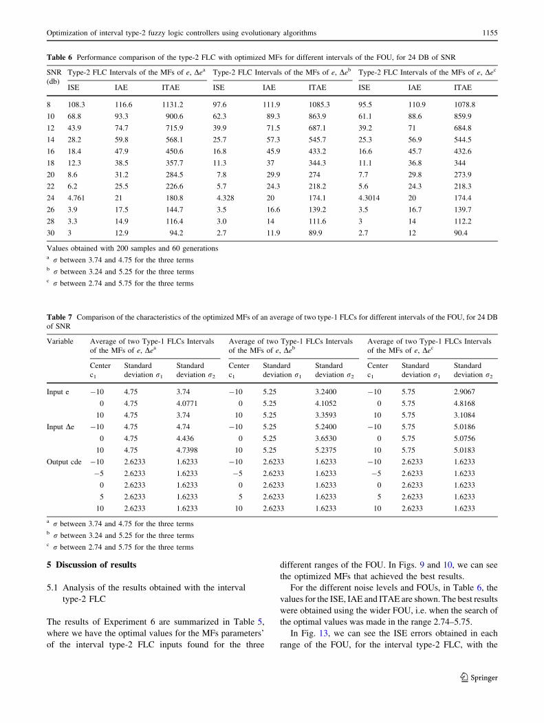
For the different noise levels and FOUs, in Table 6, the

values for the ISE, IAE and ITAE are shown. The best results

were obtained using the wider FOU, i.e. when the search of

the optimal values was made in the range 2.74–5.75.

In Fig. 13, we can see the ISE errors obtained in each

range of the FOU, for the interval type-2 FLC, with the

Table 6 Performance comparison of the type-2 FLC with optimized MFs for different intervals of the FOU, for 24 DB of SNR

SNR

(db)

Type-2 FLC Intervals of the MFs of e, Dea Type-2 FLC Intervals of the MFs of e, Deb Type-2 FLC Intervals of the MFs of e, Dec

ISE IAE ITAE ISE IAE ITAE ISE IAE ITAE

8 108.3 116.6 1131.2 97.6 111.9 1085.3 95.5 110.9 1078.8

10 68.8 93.3 900.6 62.3 89.3 863.9 61.1 88.6 859.9

12 43.9 74.7 715.9 39.9 71.5 687.1 39.2 71 684.8

14 28.2 59.8 568.1 25.7 57.3 545.7 25.3 56.9 544.5

16 18.4 47.9 450.6 16.8 45.9 433.2 16.6 45.7 432.6

18 12.3 38.5 357.7 11.3 37 344.3 11.1 36.8 344

20 8.6 31.2 284.5 7.8 29.9 274 7.7 29.8 273.9

22 6.2 25.5 226.6 5.7 24.3 218.2 5.6 24.3 218.3

24 4.761 21 180.8 4.328 20 174.1 4.3014 20 174.4

26 3.9 17.5 144.7 3.5 16.6 139.2 3.5 16.7 139.7

28 3.3 14.9 116.4 3.0 14 111.6 3 14 112.2

30 3 12.9 94.2 2.7 11.9 89.9 2.7 12 90.4

Values obtained with 200 samples and 60 generationsa r between 3.74 and 4.75 for the three termsb r between 3.24 and 5.25 for the three termsc r between 2.74 and 5.75 for the three terms

Table 7 Comparison of the characteristics of the optimized MFs of an average of two type-1 FLCs for different intervals of the FOU, for 24 DB

of SNR

Variable Average of two Type-1 FLCs Intervals

of the MFs of e, DeaAverage of two Type-1 FLCs Intervals

of the MFs of e, DebAverage of two Type-1 FLCs Intervals

of the MFs of e, Dec

Center

c1

Standard

deviation r1

Standard

deviation r2

Center

c1

Standard

deviation r1

Standard

deviation r2

Center

c1

Standard

deviation r1

Standard

deviation r2

Input e -10 4.75 3.74 -10 5.25 3.2400 -10 5.75 2.9067

0 4.75 4.0771 0 5.25 4.1052 0 5.75 4.8168

10 4.75 3.74 10 5.25 3.3593 10 5.75 3.1084

Input De -10 4.75 4.74 -10 5.25 5.2400 -10 5.75 5.0186

0 4.75 4.436 0 5.25 3.6530 0 5.75 5.0756

10 4.75 4.7398 10 5.25 5.2375 10 5.75 5.0183

Output cde -10 2.6233 1.6233 -10 2.6233 1.6233 -10 2.6233 1.6233

-5 2.6233 1.6233 -5 2.6233 1.6233 -5 2.6233 1.6233

0 2.6233 1.6233 0 2.6233 1.6233 0 2.6233 1.6233

5 2.6233 1.6233 5 2.6233 1.6233 5 2.6233 1.6233

10 2.6233 1.6233 10 2.6233 1.6233 10 2.6233 1.6233

a r between 3.74 and 4.75 for the three termsb r between 3.24 and 5.25 for the three termsc r between 2.74 and 5.75 for the three terms

Optimization of interval type-2 fuzzy logic controllers using evolutionary algorithms 1155

123

optimized parameters of the MFs. The ISE T2-1 corresponds

to the FOU range of 3.74–4.75, the ISE T-2 to the FOU range

of 3.24–4.75, and finally the ISE T-3 represents the value

when the range is from 2.74 to 5.75. The difference between

the ISE T-2 and ISE T-3 is minimum, see Table 6.

5.2 Analysis of the results obtained with the average

of two Type-1 FLCs

In order to evaluate the performance of an interval type-2

FLC using the average of two type-1 FLCs, experiment 7

was done under the same conditions of Experiment 6.

In Table 7, we show the optimal values of the MFs of

the two type-1 FLCs for each FOU search range. Fig-

ures 11 and 12 show the optimized MFs that achieved the

best results, and as in Experiment 6, they were obtained for

the wider search range.

In Table 8, we have the values for the ISE, IAE and

ITAE errors, for the different noise levels and FOU. In this

case, as in Experiment 6, the best results were obtained

with the wider FOU, in the range between 2.74 and 5.75.

Table 8 Performance comparison of the average of two type-1 FLCs with optimized MFs for different intervals of the FOU for 24 DB of SNR

values obtained with 200 samples and 60 generations

SNR (db) Average of two Type-1 FLCs

Intervals of the MFs of e, DeaAverage of two Type-1 FLCs

Intervals of the MFs of e, DebAverage of two Type-1 FLCs Intervals

of the MFs of e, Dec

ISE IAE ITAE ISE IAE ITAE ISE IAE ITAE

8 104.4 114.9 1113.1 95.6 110.8 1074.8 96.1 111 1074.4

10 66.4 91.8 886.3 61.1 88.4 855.3 61.3 88.59 854.6

12 42.4 73.5 704.5 39.1 70.7 680 39.3 70.7 679.3

14 27.3 58.8 558.9 25.2 56.6 539.9 25.3 56.6 539.3

16 17.8 47.1 443 16.5 45.4 428.5 16.5 45.3 427.9

18 11.9 37.8 351.6 11 36.5 340.5 11 36.5 339.9

20 8.2 30.6 279.5 7.6 29.5 270.9 7.6 29.5 270.4

22 6 24.9 222.5 5.5 24 215.6 5.5 23.9 215.1

24 4.5619 20.5 177.4 4.2024 19.7 171.9 4.195 19.6 171.4

26 3.7 17 141.8 3.4 16.3 137.2 3.4 16.2 136.8

28 3.2 14.4 113.8 2.9 13.7 109.9 2.9 13.6 109.5

30 2.9 12.4 92 2.6 11.6 88.4 2.6 11.6 88.1

a r between 3.74 and 4.75 for the three termsb r between 3.24 and 5.25 for the three termsc r between 2.74 and 5.75 for the three terms

Fig. 9 Optimized MFs of the input e for the type-2 FLC, for a range

of the FOU between 2.74 and 5.75Fig. 10 Optimized MFs of the input delta e of the type-2 FLC, for a

range of the FOU between 2.74 and 5.75

1156 O. Castillo et al.

123

5.2.1 Comparison of the ISE error obtained for different

FOU ranges, using the average of two Type-1 FLCs,

for each different noise level

In Figs. 13 and 14, we can see the ISE errors obtained in each

range of the FOU, for the average of two Type-1 FLCs, with

the optimized parameters of the MFs. ISE PROM-1 corre-

sponds for the range between 3.74 and 4.75 of the FOU, ISE

PROM-2 for the range 3.24 and 4.75 of the FOU, finally ISE

PROM-3 represents the value when the range is 2.74 and

5.75. In addition, in this case, the difference between the ISE

PROM-2 and ISE PROM-3 is minimal.

5.3 Comparison of the results with the interval type-2

FLC and the average of two type-1 FLCs

In order to know which system behaves in a better way in

the experiments where we simulated uncertainty through

different noise levels, we first are going to compare the

values of the ISE, IAE and ITAE errors obtained with the

optimized parameters of the MFs of the interval type-2

FLC and the average of the two type-1 FLCs. This com-

parison is made with the best results obtained with each

FLC, which, in accordance to Tables 6 and 8, correspond

to those obtained for the wider FOU. The second com-

parison is made with the standard deviation values and the

variance obtained in each optimization process to get the

Fig. 11 Optimized MFs of the input e for the average of two type-1

FLCs, for a range of the FOU between 2.74 and 5.75

Fig. 12 Optimized MFs of the input delta e for the average of two

type-1 FLCs, for a range of the FOU between 2.74 and 5.75

Fig. 13 Comparison of the ISE errors for the optimized interval type-

2 FLCs. The ISE T2-1 corresponds for a search interval of the FOU of

3.74–4.75, the ISE T2-2 for a FOU of 3.24–5.25, and the ISE T2-3 for

a FOU of 3.74–5.75, for 24 db of SNR

Fig. 14 Comparison of the ISE errors for the optimized average of

two type-1 FLCs. The ISE PROM-1 corresponds for a search interval

of the FOU of 3.74–4.75, ISE PROM2-2 for a FOU of 3.24–5.25, ISE

PROM-3 for a FOU of 3.74–5.75, for 24 db of SNR

Optimization of interval type-2 fuzzy logic controllers using evolutionary algorithms 1157

123

optimal parameters of the MFs for the minimal ISE, IAE

and ITAE errors.

5.3.1 Comparison of the ISE, IAE and ITAE errors

obtained with the interval Type-2 FLC and the

average of two Type-1 FLCs

We can see in Tables 6 and 8 that with the average of two

type-1 FLCs optimized with the wider FOU, it was

obtained a minimum advantage in the values of ISE, IAE

and ITAE errors with respect to the optimized interval

type-2 FLC under the same conditions than the type-1 for

the wider FOU. In Figs. 15, 16, and 17 it is shown that this

advantage is more significant for a low noise level.

5.3.2 Analysis of the results of the interval type-2 FLC

and the average of the two Type-1 FLCs

We can see in Table 9, the values obtained in the optimi-

zation process of the optimal parameters for the MFs after

30 tests, of the variance, the Standard deviation, best ISE

value, average ISE obtained with the optimized interval

type-2 FLC, and average ISE with the average of two

optimized type-1 FLCs.

To analyze the statistical behavior of the tests realized

with the interval type-2 FLC and the average of two type-1

FLCs, the hypothesis test using the statistical distribution

known as the t student was made, where we have the fol-

lowing hypothesis:

H0 : l1 ¼l2

H1 : l1 6¼l2

In this case, H0 corresponds to the null hypothesis and

H1 the alternative hypothesis. The intention is to show if

the average of the two type-1 FLCs could be used properly

instead of the interval type-2 FLC. This can be

demonstrated if the null hypothesis is accepted, or on the

contrary if the alternative hypothesis is rejected.

Fig. 15 Comparison of the ISE errors for optimized interval type-2

FLC and the optimized average of two type-1 FLCs, for different

noise levels. It is observed a minimal advantage of the optimized

average of two type-1 FLCs for low noise levels

Fig. 16 Comparison of the IAE errors for optimized interval type-2

FLC and the optimized average of two type-1 FLCs, for different

noise levels. They behave almost the same, but it is observed a

minimal advantage of the optimized average of two type-1 FLCs for

low noise levels

Fig. 17 Comparison of the ITAE errors for optimized interval type-2

FLC and the optimized average of two type-1 FLCs, for different

noise levels, which basically shows no difference

1158 O. Castillo et al.

123

In Table 10, it is shown that as the search interval of the

FOU increases, the average of two type-1 FLCs has the

opportunity to perform as well as the interval type-2 FLC

and can be considered as a good approximation in this

particular situation. This is concluded because the statisti-

cal values decrease in the t test as the search interval

increases, which means that both statistical processes look

almost the same. Of course, this is possible because the

optimized type-1 FLCs are used in the approximation of

the interval type-2 FLC. The advantage of this approxi-

mation is that it is simpler to implement two interval type-1

FLCs than a complete interval type-2 FLC and also the real

time responses are faster, which is needed for real world

applications. It remains to be studied if the approximation

of an interval type-2 FLC with two type-1 FLCs can be

extended to more general situations or even to other types

of problems.

In comparing the results with other ones reported in

the literature, the results presented in Tables 5, 6, 7, 8, 9,

and 10 of this paper are better than those presented in

(Sepulveda et al. 2007) for the same non-linear plant. The

main reason for this statement is that now in this paper the

optimization method has been applied to design in an

appropriate fashion the type-2 membership functions for

the problem. An optimal design of the parameter values in

the type-2 fuzzy sets is very important to achieve perfor-

mance of the fuzzy controller, which is in this case

achieved using the HEM.

6 Conclusions

We can conclude that using the ISE, IAE, and ITAE as

performance criteria that in systems without uncertainty

(ideal systems) it is a better choice to select a type-1 FLC

since it works a little better than a type-2 FLC, and it is

easier to implement it. It is also well known that a type-1

FLC can handle nonlinearities, and uncertainties up to

some extent.

In the simulation of real systems, with a higher degree of

uncertainty (for example, due to noise in measurements or

other types of noise), we can conclude that lower overshoot

errors and the best settling times are obtained using an

interval type-2 FLC. The results presented in Table 4 show

that the performance of this kind of controllers is better

under high noise levels.

We can conclude that using an interval type-2 FLC in

real world applications can be potentially a good option

since this type of system is a more suitable choice to

manage high levels of uncertainty, as we can see in the

results shown in Tables 3 and 4.

We also discovered that optimizing the membership

functions (MFs) for the inputs of an interval type-2 system

increases the performance of the system for high noise

levels. In addition, when the search interval for optimizing

the MFs is wider, we obtained better results in the per-

formance of the system, as can be seen in the ISE, IAE, and

ITAE values of Tables 7 and 8, so these results indicate

that the interval type-2 fuzzy system can handle in a better

way the uncertainty introduced to the control system.

We have also shown with statistical evidence that the

performance of the optimized average of two interval type-

1 FLCs can approximate very closely the real behavior of

an interval type-2 FLC in this particular situation, and can

be considered as a potential good approximation for real

world control applications because it is simpler to imple-

ment and can produce faster real time responses.

Finally, we can mention that the case study of control-

ling a particular non-linear plant appears to be an isolated

situation, but we think that it represents well a general class

of non-linear plants and that the results would be similar

for many cases, even for problems of other areas of

application. Of course, in control problems is where it may

be more crucial to have a quick response for real time

applications and this is when using the proposed method of

an average of two optimized type-1 fuzzy systems to

approximate an interval type-2 fuzzy system may be more

Table 9 Comparison of the variance, the standard deviation, best ISE value, ISE average, obtained with the optimized interval type-2 FLC and

the optimized average of two type-1 FLCs

Search

Interval

Type-2 FLC Average of two Type-1 FLCs

Best ISE value ISE Average Standard deviation Variance Best ISE value ISE Average Standard deviation Variance

3.74–4.75 4.761 4.9942 0.1649 0.0272 4.5619 4.7701 0.1498 0.0224

3.24–5.25 4.328 4.5060 0.1460 0.0213 4.2024 4.4009 0.1568 0.0246

2.74–5.75 4.3014 4.4005 0.1653 0.0273 4.1950 4.3460 0.1424 0.0203

Table 10 Results of the t-student test

Search interval t0 tpdf_r

3.74–4.75 5.5096 1.6384 9 10-6

3.24–5.25 2.6869 0.0125

2.74–5.75 1.3682 0.1556

Optimization of interval type-2 fuzzy logic controllers using evolutionary algorithms 1159

123

important. We leave as future work the task of considering

more general cases and or other types of application for this

proposed approximation of interval type-2 fuzzy systems.

References

Castillo O, Melin P (2001) Soft computing for control of non-linear

dynamical systems. Springer, Heidelberg

Castillo O, Melin P (2003) Soft computing and fractal theory for

intelligent manufacturing. Springer, Heidelberg

Castillo O, Melin P (2004) A new approach for plant monitoring

using type-2 fuzzy logic and fractal theory. Int J Gen Syst

33:305–319

Castillo O, Melin P (2007) Type-2 fuzzy logic: theory and applica-

tions. Springer, Heidelberg

Castillo O, Melin P (2008) Intelligent systems with interval type-2

fuzzy logic. Int J Innovat Comput Inf Control 4:771–783

Castro JR, Castillo O, Melin P, Rodriguez-Diaz A (2009) A hybrid

learning algorithm for a class of interval type-2 fuzzy neural

networks. Inf Sci 179:2175–2193

Deb K (2002) Multi-objective optimization using evolutionary

algorithms. Wiley, Great Britain

Deshpande PB, Ash RH (1988) Computer process control with

advanced control applications. Instrument Society of America,

USA

Hagras HA (2004) Hierarchical type-2 fuzzy logic control architec-

ture for autonomous mobile robots. IEEE Trans Fuzzy Syst

12:524–539

Ingle VK, Proakis JG (2000) Digital signal processing using

MATLAB. Brooks/Cole Publishing Company

Jang JSR, Sun CT, Mizutani E (1997) Neuro-fuzzy and soft

computing, a computational approach to learning and machine

intelligence, Matlab Curriculum Series. Prentice Hall, New

Jersey

Karnik NN, Mendel JM (1999) Applications of type-2 fuzzy logic

systems to forecasting of time-series. Inf Sci 120:89–111

Karnik NN, Mendel JM (2001a) Operations on type-2 fuzzy sets. Int J

Fuzzy Sets Syst 122:327–348

Karnik NN, Mendel JM (2001b) Centroid of a type-2 fuzzy set. Inf

Sci 132(1–4):195–220

Karnik NN, Mendel JM, Liang Q (1999) Type-2 fuzzy logic systems.

IEEE Trans Fuzzy Syst 7:643–658

Karnik NN, Liang Q, Mendel JM (2001) Type-2 fuzzy logic software.

Available online at http://sipi.usc.edu/mendel/software/

Klir GJ, Yuan B (1995) Fuzzy sets and fuzzy logic: theory and

applications. Prentice Hall, New York

Kumar P, Bauer P (2009) Progressive design methodology for

complex engineering systems based on multiobjective genetic

algorithms and linguistic decision making. Soft Comput 13:649–

679

Liang Q, Mendel JM (2000) Interval type-2 fuzzy logic systems:

theory and design. IEEE Trans Fuzzy Syst 8:535–550

Mamdani EH (1993) Twenty years of fuzzy control: experiences

gained and lessons learn. In: Marks RJ (ed) Fuzzy Logic

Technology and Applications. IEEE Press, New Jersey

Martinez R, Castillo O, Aguilar LT (2009) Optimization of interval

type-2 fuzzy logic controllers for a perturbed autonomous

wheeled mobile robot using Genetic Algorithms. Inf Sci

179:2158–2174

Melin P, Castillo O (2002) Intelligent control of non-linear dynamic

plants using type-2 fuzzy logic and neural networks. In:

Proceedings of the Annual Meeting of the North American

Fuzzy Information Processing Society

Melin P, Castillo O (2003) A new method for adaptive model-based

control of non-linear plants using type-2 fuzzy logic and neural

networks intelligent control of non-linear dynamic plants using

type-2 fuzzy logic and neural networks. In: Proceedings of the

12th IEEE conference on fuzzy systems

Melin P, Castillo O (2004) A new method for adaptive control of non-

linear plants using type-2 fuzzy logic and neural networks. Int J

Gen Syst 33:289–304

Mendel JM (1998) Type-2 fuzzy logic systems: type-reduction. In:

Proceedings of IEEE syst., man, cybern. conf., San Diego

Mendel JM (1999) Computing with words, when words can mean

different things to different people. In: Int. ICSC Congress

Computat. Intell. Methods Applications, Rochester, New York

Mendel JM (2000) Uncertainty, fuzzy logic, and signal processing.

Signal Process J 80:913–933

Mendel JM (2001) Uncertain rule-based fuzzy logic systems:

introduction and new directions. Prentice Hall, New York

Mendel JM (2005) On a 50% savings in the computation of the

centroid of a symmetrical interval type-2 fuzzy set. Inf Sci

172:417–430

Mendel JM, John RI (2002) Type-2 fuzzy sets made simple. IEEE

Trans Fuzzy Syst 10:117–127

Mendel JM, Mouzouris GC (1999) Type-2 fuzzy logic systems. IEEE

Trans Fuzzy Syst 7:643–658

Mizumoto M, Tanaka K (1976) Some properties of fuzzy sets of type-

2. Inf Control 31:312–340

Montiel O, Castillo O, Melin P, Diaz AR, Sepulveda R (2007) Human

evolutionary model: a new approach to optimization. Inf Sci

177(10):2075–2098

Ozen T, Garibaldi JM (2003) Investigating adaptation in type-2 fuzzy

logic systems applied to umbilical acid-base assessment. In:

European symposium on intelligent technologies, hybrid systems

and their implementation on smart adaptive systems (EUNITE

2003), Oulu, Finland

Sepulveda R, Castillo O, Melin P, Rodriguez-Diaz A, Montiel O

(2007) Experimental study of intelligent controllers under

uncertainty using type-1 and type-2 fuzzy logic. Inf Sci

177:2023–2048

Yager RR (1980) Fuzzy subsets of type II in decisions. J Cybern

10:137–159

Zadeh LA (1971) Similarity relations and fuzzy ordering. Inf Sci

3:177–206

Zadeh LA (1973) Outline of a new approach to the analysis of

complex systems and decision processes. IEEE Trans Syst Man

Cybern 3:28–44

Zadeh LA (1975a) The concept of a linguistic variable and its

application to approximate reasoning. Inf Sci 8:43–80

Zadeh LA (1975b) The concept of a linguistic variable and its

application to approximate reasoning, Part 1. Inf Sci 8:199–249

1160 O. Castillo et al.

123